Abstract

The organising principles underlying the structure of phenomenologically viable string vacua can be accessed by sampling such vacua. In many cases this is prohibited by the computational cost of standard sampling methods in the high dimensional model space. Here we show how this problem can be alleviated using reinforcement learning techniques to explore string flux vacua. We demonstrate in the case of the type IIB flux landscape that vacua with requirements on the expectation value of the superpotential and the string coupling can be sampled significantly faster by using reinforcement learning than by using metropolis or random sampling. Our analysis is on conifold and symmetric torus background geometries. We show that reinforcement learning is able to exploit successful strategies for identifying such phenomenologically interesting vacua. The strategies are interpretable and reveal previously unknown correlations in the flux landscape.

1 Introduction

The string theory flux landscape covers a vast range of low-energy effective field theories [1, 2, 3]. A subset of such theories might be phenomenologically desirable, e.g. featuring a weak string coupling $g_{s}$ and a particular scale of supersymmetry breaking $m_{3/2}$, largely determined by the expectation value of the flux superpotential $W_{0}.$

Apriori, it is unclear whether such phenomenological structures single out a particular subset of flux configurations and what the common features are in the UV representation. By sampling the space of flux vacua such properties can be revealed. Although in few parameter models an exploration via random or even complete sampling is tractable, more realistic models require a different sampling strategy. In fact it has been argued that the computational complexity of finding flux vacua is NP hard [24, 25, 26] but phenomenologically relevant vacua can nevertheless be found with appropriate optimisation techniques [27]. More widely speaking advances in artificial intelligence techniques make it possible to analyse this problem with a variety of approaches (cf. [28] for an overview).

Here, we exemplify for the first time how reinforcement learning (RL) can be used to search for such correlations in the flux landscape (see [29] for a classic textbook on RL). RL has previously been utilised to identify efficiently models of particles physics from string theory [30, 31, 32].

For simplicity and, in addition, to compare with other sampling approaches we restrict this analysis to few parameter examples which also have been analysed with the help of genetic algorithms [33]. We are able to show that RL can outperform metropolis sampling in efficiency in this context. Both approaches reveal correlations among flux quanta – previously unreported in the literature to our knowledge. Our RL agents however have learned to explore the flux environment such that they can navigate in nearby solution space, i.e. to remain in the fundamental domain and to keep a particular scale of supersymmetry breaking.

The rest of the paper is organised as follows. In Section 2 we describe the flux examples, how the RL environment is generated and which reward structure is visible. Section 3 contains our main analysis of these examples and compares the performance of RL approaches with metropolis and random searches. In Section 4 we conclude. Details on the RL algorithms we use can be found in Appendix A, our hyperparameter searches can be found in Appendix B, and more experiments on the torus background are summarised in Appendix C.

2 Flux environments

At this stage our analysis is based on fixed background geometries. Here we set the necessary notation and introduce the two environments we use for our analysis, the weighted projective space $\textbf{WP}^{4}_{1,1,1,1,4}$ which we analyse near its conifold locus and the symmetric torus $T^{6}$ both with one complex structure modulus. Both are chosen as simple toy examples and as they allow for a comparison with the performance of genetic algorithms on these environments [33].

2.1 Flux datasets

We consider a Calabi-Yau threefold $M$ with $h_{2,1}$ complex structure moduli and take s symplectic basis $\{A^{a},B_{b}\}$ for the $b_{3}=2(h_{2,1}+1)$ three-cycles, with $a,b=1,\dots,h_{2,1}.$ The cohomology elements $\alpha_{a},\beta^{b}$ dual to our basis satisfy

$$\int_{A^{a}}\alpha_{b}=\delta_{b}^{a}\ ,\qquad\int_{B_{b}}\beta^{a}=-\delta^{a}_{b}\ ,\qquad\int_{M}\alpha_{a}\wedge\beta^{b}=\delta_{a}^{b}\ .$$ (1)

The holomorphic three form $\Omega$, unique to our Calabi-Yau threefold, defines the periods
$z^{a}=\int_{A^{a}}\Omega,$ $\mathcal{G}_{b}=\int_{B_{b}}\Omega$ and leads to the $b_{3}$-vector $\Pi(z)=(\mathcal{G}_{b},z^{a})$. It can also be written as $\Omega=z^{a}\alpha_{a}-\mathcal{G}_{a}\beta^{a}$. The Kähler potential for the complex structure moduli and the axio-dilaton $\phi=C_{0}+ie^{-\varphi}$ is

$$\mathcal{K}=-\text{log}\left(i\int_{M}\Omega\wedge\bar{\Omega}\right)-\text{log}\left(-i(\phi-\bar{\phi})\right)=-\text{log}\left(-i\leavevmode\nobreak\ \Pi^{\dagger}\cdot\Sigma\cdot\Pi\right)-\text{log}\left(-i(\phi-\bar{\phi})\right)\ ,$$ (2)

since

$$\int_{M}\Omega\wedge\bar{\Omega}=\bar{z}^{a}\mathcal{G}_{a}-z^{a}\bar{\mathcal{G}}_{a}=-\Pi^{\dagger}\cdot\Sigma\cdot\Pi\ ,$$

with the symplectic matrix

$$\Sigma=\left(\begin{array}[]{c c}0&{\bf 1}\\ -{\bf 1}&0\end{array}\right)\ .$$ (3)

Turning on RR and NSNS 3-form fluxes leads to the quantized flux vectors in the $\alpha,\beta$ basis as

$$F_{3}=-(2\pi)^{2}\alpha^{\prime}(f_{a}\alpha_{a}+f_{a+h_{2,1}+1}\beta^{a}),\quad H_{3}=-(2\pi)^{2}\alpha^{\prime}(h_{a}\alpha_{a}+h_{a+h_{2,1}+1}\beta^{a})\ ,$$ (4)

where $f$ and $h$ are integer-valued $b_{3}$-vectors. In the following we set $(2\pi)^{2}\alpha^{\prime}=1$ . The background fluxes introduce a superpotential [37]

$$W=\int_{M}(F_{3}-\phi H_{3})\wedge\Omega(z)=(f-\phi h)\cdot\Pi(z)$$ (5)

and a scalar potential

$$V=e^{\mathcal{K}}(\mathcal{K}^{i\bar{\jmath}}D_{i}WD_{\bar{\jmath}}\bar{W}-3|W|^{2})\ .$$ (6)

The $\mathcal{K}^{i\bar{\jmath}}$ is the inverse of the Kähler metric and $D_{i}W=(\partial_{i}+(\partial_{i}\mathcal{K}))W.$ Here, the indices $i,\bar{\jmath}$ run over the complex structure moduli, the dilaton and the Kähler moduli. Due to the leading order no-scale structure for the Kähler moduli their contribution to the scalar potential cancels the $3|W|^{2}$ term and we end up with a positive semi-definite scalar potential

$$V=e^{\mathcal{K}}(\mathcal{K}^{a\bar{b}}D_{a}WD_{\bar{b}}\bar{W}+\mathcal{K}^{\phi\bar{\phi}}D_{\phi}WD_{\bar{\phi}}\bar{W})\ .$$ (7)

Here, the indices $a,\bar{b}$ only include the complex structure moduli and $\phi$ is the axio-dilaton. We are interested in vacua which have vanishing scalar potential (Minkowski vacua and fulfil the so called imaginary self-dual (ISD) condition). Hence we are looking for vanishing F-terms

$$D_{\phi}W = \frac{1}{\bar{\phi}-\phi}(f-\bar{\phi}h)\cdot\Pi(z)=0\ ,$$

$$D_{a}W = (f-\phi h)\cdot(\partial_{a}\Pi(z)+\Pi(z)\partial_{a}\mathcal{K})=0\ .$$ (8)

The fluxes contribute to the D3-brane charge via

$$N_{\text{flux}}=\int_{M}F_{3}\wedge H_{3}=f\cdot\Sigma\cdot h\ .$$ (9)

For ISD fluxes we have $N_{\text{flux}}>0$. Since the total D3-brane charge on a compact manifold has to vanish and to ensure tadpole cancellation, appropriate negative charges have to be added (e.g. by orientifolding). Effectively this introduces an upper bound on $N_{\text{flux}}$ [33, 34]:

$$0<N_{\text{flux}}<L_{\text{max}}\ ,$$ (10)

where $L_{\rm max}$ is model dependent and we will utilise the same values as in [33] to keep comparability. We combine our fluxes into the flux vector

$$N=(f_{1},\dots,f_{2h_{2,1}+2},h_{1},\dots,h_{2h_{2,1}+2})^{T}\ .$$ (11)

In summary, we search for flux vectors with $0<N_{\text{flux}}<L_{\rm max}$ and which yield vacua with vanishing scalar potential and additional phenomenological constraints on the expectation value for the dilaton and the superpotential. For this calculation, we now specify background geometries where we can calculate the period vector $\Pi(z)$ which allows us to calculate and solve the F-term conditions for the dilaton and complex structure moduli (8). Given them, we can go on to calculate explicitly the expectation values for the superpotential and the string coupling. In addition, the scalar potential is invariant under an $SL(2,\mathbb{Z})$ symmetry which acts non-trivially on the dilaton and the flux vectors. To avoid the resulting over-counting we restrict ourselves to dilaton values which lie in the fundamental domain that is

$$\{\phi\}:=\{\phi:|\text{Re}(\phi)|<0.5,\ |\phi|>1\}\ .$$ (12)

Explicit background: Conifold in $\textbf{WP}^{4}_{1,1,1,1,4}$

For the first experiments, we will work on a conifold described as a hypersurface in the weighted projective space $\textbf{WP}^{4}_{1,1,1,1,4}$ defined by

$$\sum_{i=1}^{4}x_{i}^{8}+4x_{0}^{2}+8\psi x_{0}x_{1}x_{2}x_{3}x_{4}=0\ .$$ (13)

The Hodge numbers here are given by $h_{1,1}=1$ and $h_{2,1}=149$. We will consider the case of the orientifold $x_{0}\rightarrow-x_{0}$, $\psi\rightarrow-\psi$ with worldsheet parity reversal that arises from F-theory compactified on a Calabi-Yau fourfold defined as a hypersurface $X_{A}=\textbf{WP}^{5}_{1,1,1,1,8,12}$ . Because of that special property, the tadpole can be calculated from the Euler characteristic of the fourfold to be [38]

$$L_{\text{max}}=\frac{\chi(X_{A})}{24}=\frac{23328}{24}=972\ ,$$ (14)

which sets the maximal tadpole for our flux configurations. This conifold (13) has a symmetry group $\Gamma=\mathbb{Z}^{2}_{8}\times\mathbb{Z}_{2}$ under which all complex structure deformations are charged except $\psi$. Hence if we only turn on fluxes consistent with $\Gamma$, these charged moduli can be dropped and the periods can be calculated only for the axio-dilaton $\phi$ and the uncharged modulus $\psi$ [38]. Since we only have one complex structure modulus, the flux vector (11) is 8-dimensional and given by $N=(f_{1},f_{2},f_{3},f_{4},h_{1},h_{2},h_{3},h_{4})^{T}$. Near the conifold point $\psi=1$ the periods are [39]

$$\mathcal{G}_{1}(x) = (2\pi i)^{3}(a_{0}+a_{1}x+\mathcal{O}(x^{2}))\ ,$$

$$\mathcal{G}_{2}(x) = \frac{z^{2}(x)}{2\pi i}\text{ln}(x)+(2\pi i)^{3}(b_{0}+b_{1}x+\mathcal{O}(x^{2}))\ ,$$

$$z^{1}(x) = (2\pi i)^{3}(c_{0}+c_{1}x+\mathcal{O}(x^{2}))\ ,$$

$$z^{2}(x) = (2\pi i)^{3}(d_{0}+d_{1}x+\mathcal{O}(x^{2}))\ ,$$

with $x=1-\psi,|x|\ll 1$ [39]. The constants are given as

$$a_{0} = -1.774i,\quad a_{1}=1.227\ ,$$

$$b_{0} = -1.047,\quad b_{1}=0.451+0.900i\ ,$$

$$c_{0} = 4.952-5.321i,\quad c_{1}=-4.488+3.682i\ ,$$

$$d_{0} = 0.000,\quad d_{1}=1.800i\ .$$ (15)

Solving the F-term conditions (8) for the dilaton and complex structure modulus leads to [39]

$$\phi = \frac{f_{1}\bar{a}_{0}+f_{2}\bar{b}_{0}+f_{3}\bar{c}_{0}}{h_{1}\bar{a}_{0}+h_{2}\bar{b}_{0}+h_{3}\bar{c}_{0}}+\mathcal{O}(|x|\text{ln}(|x|))\ ,$$

$$\text{ln}(x) = -\frac{2\pi i}{d_{1}}\Biggl{(}\frac{(f_{1}-\phi h_{1})(a_{1}-\frac{\mu_{1}}{\mu_{0}}a_{0})+(f_{2}-\phi h_{2})(b_{1}-\frac{\mu_{1}}{\mu_{0}}b_{0})}{f_{2}+\phi h_{2}}$$ (16)

$$\qquad\qquad+\frac{(f_{3}-\phi h_{3})(c_{1}-\frac{\mu_{1}}{\mu_{0}}c_{0})+(f_{4}-\phi h_{4})d_{1}}{f_{2}-\phi h_{2}}\Biggr{)}-1\ .$$

with

$$\mu_{0}=i(2\pi)^{6}(a_{0}\bar{c}_{0}-c_{0}\bar{a}_{0}),\quad\mu_{1}=i(2\pi)^{6}(\bar{c}_{0}a_{1}-c_{1}\bar{a}_{0}-d_{1}\bar{b}_{0})\ .$$ (17)

In this conifold background we are interested in vacua with a fixed absolute value for the expectation value of the flux superpotential $|W_{0}|=50,000.$ The motivation behind choosing such an artificial value is to estimate the ability to find vacua with nearby values. Such a tuning would for instance be required in tuning the cosmological constant in a LARGE volume scenario [40].

In addition, for this value of the flux superpotential solutions are easily found even by random algorithms and it corresponds to the value the genetic algorithms in [33] have focused on.

Background geometry: symmetric torus

The second background in our experiments is the symmetric $T^{6}$ torus. We are also interested in specific values of the superpotential $W_{0}$ and in specific values for the string coupling $g_{s}.$ We follow the conventions of [34].
Since the considered torus is symmetric, it can be viewed as a direct product of three copies of $T^{2}$ and here we only have one complex structure modulus. Taking the axio-dilaton into account we get two moduli and in total 8 independent flux parameters. First, consider a non symmetric general $T^{6}$. The coordinates $x^{i},y^{i}$ for $i=1,2,3$ with periodicity $x^{i}\sim x^{i}+1,\leavevmode\nobreak\ y^{i}\sim y^{i}+1$ are defined such that the holomorphic 1-forms can be written as $dz^{i}=dx^{i}+\tau^{ij}dy^{j}$ with the complex structure moduli $\tau^{ij}$. The orientation is

$$\int\ dx^{1}\wedge dx^{2}\wedge dx^{3}\wedge dy^{1}\wedge dy^{2}\wedge dy^{3}=1$$

and the symplectic basis for $H^{3}(T^{6},\mathbb{Z})$ is

$$\alpha^{0} = dx^{1}\wedge dx^{2}\wedge dx^{3}\ ,\qquad\alpha_{ij}=\frac{1}{2}\epsilon_{ilm}dx^{l}\wedge dx^{m}\wedge dy^{j}\ ,$$

$$\beta^{ij} = -\frac{1}{2}\epsilon_{jlm}dy^{l}\wedge dy^{m}\wedge dx^{i}\ ,\qquad\beta^{0}=dy^{1}\wedge dy^{2}\wedge dy^{3}\ .$$ (18)

The holomorphic 3-form is given by

$$\Omega=dz^{1}\wedge dz^{2}\wedge dz^{3}\ .$$

With this the 3-form fluxes can be expanded in terms of the symplectic basis

$$F_{3} = a^{0}\alpha^{0}+a^{ij}\alpha_{ij}+b_{ij}\beta^{ij}+b_{0}\beta^{0}\ ,$$

$$H_{3} = c^{0}\alpha^{0}+c^{ij}\alpha_{ij}+d_{ij}\beta^{ij}+d_{0}\beta^{0}\ .$$ (19)

Now if we focus on the symmetric $T^{6}$ the complex structure moduli are all equal and we get

$$\tau^{ij}=\tau\delta^{ij}\ .$$

In this case we now only have two moduli in total and the number of fluxes gets reduced as well and we have

$$a^{ij}=a\delta^{ij}\leavevmode\nobreak\ ,\quad b_{ij}=b\delta_{ij}\leavevmode\nobreak\ ,\quad c^{ij}=c\delta^{ij}\leavevmode\nobreak\ ,\quad d_{ij}=d\delta_{ij}\ .$$ (20)

The superpotential then only depends on the two moduli and takes the form

$$W=P_{1}(\tau)-\phi P_{2}(\tau)$$ (21)

with the polynomials

$$P_{1}(\tau) = a^{0}\tau^{3}-3a\tau^{2}-3b\tau-b_{0}\ ,$$

$$P_{2}(\tau) = c^{0}\tau^{3}-3c\tau^{2}-3d\tau-d_{0}\ .$$ (22)

The Kähler potential simply is

$$\mathcal{K}=-3\log(-i(\tau-\bar{\tau}))-\log(-i(\phi-\bar{\phi}))$$ (23)

and with this the F-term constraints are

$$P_{1}(\tau)-\bar{\phi}P_{2}(\tau) = 0\ ,$$ (24)

$$P_{1}(\tau)-\phi P_{2}(\tau) = (\tau-\bar{\tau})(P_{1}^{\prime}(\tau)-\phi P_{2}^{\prime}(\tau))\ .$$ (25)

Solving Equation (24) for the dilaton leads to

$$\phi=\frac{\overline{P_{1}(\tau)}}{\overline{P_{2}(\tau)}}\ .$$ (26)

The complex structure modulus $\tau=x+iy$ is then obtained by plugging this into (25). This leads to the equations

$$q_{1}(x)y^{2} = q_{3}(x)\ ,$$ (27)

$$q_{0}(x)y^{4} = q_{4}(x)\ .$$ (28)

Eliminating $y$ and solving for $x$ leads to the cubic equation

$$\alpha_{3}x^{3}+\alpha_{2}x^{2}+\alpha_{1}x+\alpha_{0}=0\ .$$ (29)

The exact form of the polynomials $q_{i}$ and the coefficients $\alpha_{i}$ can be found in [34]. Since this equation is cubic, there will be up to three solutions for the moduli and hence up to three solutions for the superpotential as well. They are all equally valid and the algorithm will later on check all three of them. The D3-brane charge induced by the fluxes is

$$N_{flux}=b_{0}c^{0}-a^{0}d_{0}+3(bc-ad)\ .$$ (30)

As on the conifold we have to look for solutions where the dilaton lies in the fundamental domain (cf. Equation (12)). For the tadpole cancellation, one common orientifold for the torus is $T^{6}/\mathbb{Z}_{2}$ which has 64 O3-planes and hence $L_{\text{max}}=16$ [5]. We choose to work with $0<N_{\text{flux}}<16$ here. For the superpotential, we will look for values $|W_{0}|<10$ and we will also perform experiments to search for $g_{s}\approx 0.3$.

2.2 RL environment and reward structure

We are interested in exploring the flux vacua in these two background geometries. To explore them with RL we have to specify how we can navigate between various flux vacua.

We implement these environments with the use of OpenAI gym [41]. For that purpose we overwrite the following three functions:

• step: The function to actually move through the environment. It takes a specific action and a state as an input and uses it to transition to a new state. This state is then returned together with the reward for that transition and an indication whether the episode is over and if all conditions were satisfied.

• reset: The function to reset the environment to its initial configuration. This will be called at the beginning of each episode.

• seed: The function to seed the random number generators. Having a seed will give the same sequence of random numbers for the same initial data.

Gym comes with two possible spaces, a continuous Box space and a discrete Discrete space. We will define the state space as an 8 dimensional Discrete space, which corresponds to our flux vector in equation (11). The action space will be a 16 dimensional Discrete space, since we allow the agent to raise or lower one of the flux quanta in the flux vector by $\pm 1$. So for example action $a=2$ will raise the second entry of the flux vector by one and action $a=10$ will lower that entry by one. The last thing to define are the reward functions.

Reward functions

Throughout the experiments the reward functions were changed to improve performance. Here we present the general idea and describe later our hyperparameter tuning. As mentioned earlier, three conditions are checked for all of which we introduce a reward:

1. Gauge condition: $\phi\in\{\phi:|\text{Re}(\phi)|<0.5,\ |\phi|>1\}$ dilaton in fundamental domain.

2. Tadpole condition: whether $0<N_{\text{flux}}<972$ on the conifold or $0<N_{\text{flux}}<16$ on the torus.

3. Superpotential condition: $|W_{0}|=50000\pm 1000$ on the conifold and $|W_{0}|<10$ on the torus.

For fulfilling the gauge and the superpotential conditions, a fixed reward $r_{\text{gauge}}$ and $r_{\text{sup}}$ respectively is given. For not fulfilling the tadpole condition, a negative reward (punishment) $-r_{\text{tad}}$ is given. Hence the agent receives a maximal reward of $r_{\text{gauge}}+r_{\text{sup}}$. Since all of these conditions are hard to satisfy, the agent will receive no feedback whatsoever during his exploration of the environment. To avoid this and hence speed up learning, rewards (or punishments) were given proportional to the distance to the optimal solution. In more detail they look like

$$r_{g} = \begin{cases}N_{g}\cdot\par\text{exp}\left(-\left(\frac{|\text{Re}(\phi)|-0.5}{\sigma_{g}}\right)^{2}\right)\cdot r_{\rm gauge}\ &\text{if Im}(\phi)>1\ ,\\ N_{g}\cdot\par\text{exp}\left(-\left(\frac{|\text{Re}(\phi)|-0.5}{\sigma_{g}}\right)^{2}\right)\cdot\par\par\text{exp}\left(-\left(\frac{\text{Im}(\phi)-1}{\sigma_{g}}\right)^{2}\right)\cdot r_{\rm gauge}\ &\text{else}\ ,\end{cases}$$ (31)

$$r_{t} = N_{t}\cdot\text{tanh}\left(\sigma_{t}\left(N_{\text{flux}}-0\right)\right)\cdot r_{\text{tad}}\ ,$$ (32)

$$r_{s} = N_{s}\cdot\text{exp}\left(-\left(\frac{|W_{0}|-50000}{\sigma_{s}}\right)^{2}\right)\ ,$$ (33)

with normalization constants $N_{i}$ and standard deviations $\sigma_{i}$. The latter control how far away from the optimal solution a state can be and still be rewarded. There are a few things to note here. First, it is hard to define a distance from the fundamental domain. Therefore, we just choose this product of individual distances. Second the tadpole punishment is given as a tanh function, since here the punishment should get smaller the closer one gets to the optimal solution. The distance is only calculated to 0 because states with a tadpole larger then 972 are basically not present. Third, in the superpotential distance reward $r_{s}$ the exponential is not multiplied with the superpotential reward $r_{\text{sup}}$. If a correct superpotential value is found, the episode is ended. Hence, a state with a correct superpotential value is a terminal state. If the difference in reward between the terminal state and the state before is too small, it would be more rewarding for the agent to run around that terminal state forever never hitting it and hence never finding an optimal solution. To ensure that this reward difference is big enough, the exponential in $r_{s}$ is not multiplied with $r_{\text{sup}}$.

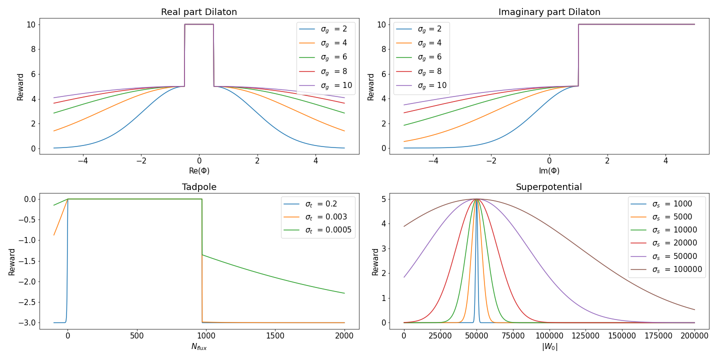
Figure 1: Reward function for different $\sigma$ values. The first two plots show the reward functions for the real and imaginary part of the dilaton, while the third one shows the tadpole and the last shows the superpotential. The $\sigma$’s have to be chosen to balance between distinguishing states near the maximum and still covering a large area of possible values for the physical quantities. For the superpotential the agent receives a fixed reward of 7000 if $49000<|W_{0}|<51000$.

The reward functions for different $\sigma$ values are shown in Figure 1. When choosing the $\sigma$ value, we have to balance between a large enough value to make sure that a large part of the environment is rewarded and a small enough value to still distinguish different states near the optimal solution.

RL agents and neural networks

We use an advantage actor-critic agent (A3C) [42] and double deep Q-learning with prioritized experience replay and duelling extensions [43, 44, 45, 46]. A short introduction to these algorithms can be found in Appendix A. For more details about reinforcement learning see [29]. We use a dense network for all of our experiments, which is inspired by [30]. It consists of four hidden layers, each with ReLu activation. For the A3C setup the activation function for the output layer of the policy network will be a softmax function to get probabilities for each action. The output will be a vector with dimension corresponding to the number of actions so each entry corresponds to one specific action. The first three layers have size 50 while the last layer has size 200.

3 Experiments/Explorations

Our RL experiments have been designed with the following scope. We are interested whether our RL agents are able to learn what successful vacua are and whether they can reveal structures on the space of vacua. Such structures will be in correlations among the flux quanta and how the RL agent navigates through the flux environment starting from a random starting point. As these RL methods are computationally more demanding than standard random or metropolis algorithms, we compare the efficiency of these three approaches. For this comparison we present our best working agents on the conifold environment. We present the results of our experiments for the metropolis algorithm, random walker, A3C and DDQN with prioritized experience replay and duelling extensions.

Our training proceeds as follows. A model is found, if all of the three conditions mentioned earlier in section 2 (gauge, tadpole, superpotential) are satisfied. The agents are run for a given number of steps $N_{\text{steps}}$ and reset if this step number is reached or a model is found. A step corresponds to one call of the step function in the environment that means a transition from one state to another e.g. going from $N=[1,0,0,0,0,0,0,0]$ to $N=[2,0,0,0,0,0,0,0]$. This will be repeated for a number of episodes $N_{\text{episode}}$. Successful models can be distinguished by their final flux vector as we are restricting ourselves to vacua in the fundamental domain. All fluxes are initialized in the interval $[-30,30]$ where the starting point is drawn from a uniform distribution.

To specify the A3C we have to choose certain hyperparameters. We used for the learning rate $l_{r}=5\cdot 10^{-4}$, for the discount factor $\gamma=0.95$ and for the exploration parameter $\beta=0.1$.

For prioritized duelling DDQN we use the learning rate $l_{r}=5\cdot 10^{-6}$ and discount factor $\gamma=0.999$. The other relevant parameters are $\alpha=0.1\ ,\beta=0.6$ for prioritized experience replay and $\epsilon_{\text{end}}=0.01\ ,\epsilon_{\text{decay}}=0.999$ for the epsilon greedy strategy. More details can be found in Appendix A.

Our RL results will always be compared to a random walker and a metropolis algorithm which both were run under the same circumstances as the plotted agents meaning with the same number of steps and the same reward structures. The random walker just chooses a random action at each step. In case of the metropolis algorithm, the agent chooses an action at random as well, but only transitions to the next state to which this action would lead to, if the reward of that state is higher than the one for the state he currently is in. If the reward is lower, the transition only happens with a probability depending on the difference in rewards

$$P=e^{-(r_{s+1}-r_{s})}\ .$$ (34)

To establish a basis of comparison let us first describe the explorations with the random walker and a metropolis algorithm. In general they both behave completely random meaning that no structure in the flux values is visible. However, if we only focus on the successful runs meaning the ones where a good vacuum was found, the situation changes. In that case we show the occupation number in our runs in Figure 2.

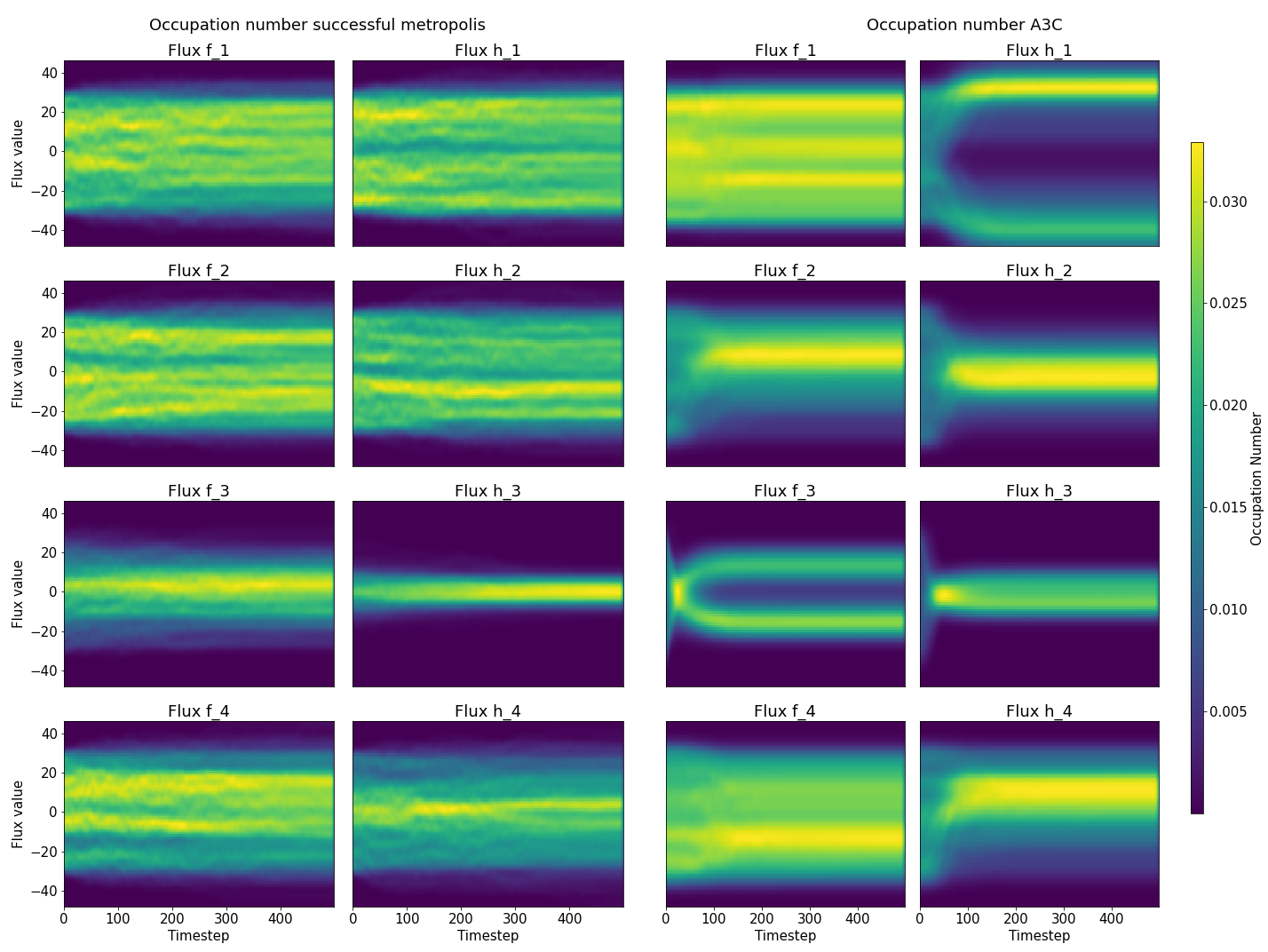
Figure 2: Here the occupation number of each flux value is shown for the successful metropolis runs and the A3C. Every plot corresponds to a flux number. Then the colour represents how often, in 500 runs, a given value of this flux number occurred at a given timestep. The flux values for the algorithms were initialized between -30 and 30.

We depict the occupation number

$$O_{i,j}(t)=\frac{N_{i,j}(t)}{N_{a}(t)}\ ,$$ (35)

where $N_{a}(t)$ is the total number of agents at timestep $t$ and $N_{i,j}(t)$ the number of agents which reach the flux value $i$ of flux number $f_{j}$ or $h_{j}$ at timestep $t$. Here $N_{a}(0)=500$ hence 500 runs where done. We find that $h_{3}$ is oriented more closely towards zero.

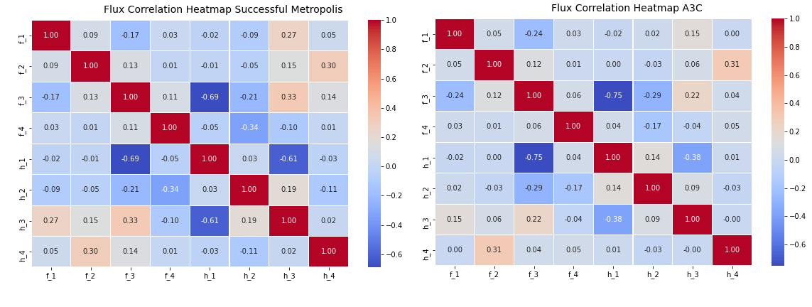
Figure 3: This plot shows the correlation heatmap of the different flux numbers for the successful metropolis algorithm and the A3C. The value in each entry is just the correlation between all encountered flux values of this flux numbers. A positive value and red colour means that the two fluxes are correlated whereas blue and negative means they are anti-correlated.

More structure can be seen in the plot from our A3C agents. The agents seems to not touch $f_{1}$ and $f_{4}$ at all, whereas $f_{2}$ is kept a little bit above zero, $h_{2}$ a little bit below zero, and $h_{3}$ around zero while $h_{4}$ is raised most of the times. With the correlation map in mind, we can safely say that $f_{3}$ and $h_{1}$ are pushed to opposite high or low values. $f_{3}$ and $h_{1}$ are pushed to opposite high or low values which we confirm below when we discuss the correlations among the flux quanta. In general, the heat map has similarities with the metropolis one where only the successful runs were plotted but features additional structures.

Correlations among the flux vacua of vacua can be seen in the correlation heat map shown in Figure 3. Here we find a strong anti-correlation between $f_{3}$ and $h_{1}$ as the most dominant feature. These correlations in phenomenologically interesting vacua have not been pointed out before.

Since these structures only appear for successful runs, we conclude that they are inherent environmental features.

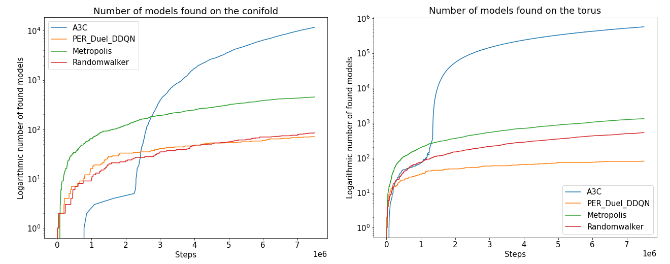
Figure 4: Comparison of log number of distinct models found per 1000 Episodes of A3C with PER dueling DDQN. A3C shows the best and fastest learning behaviour whereas PER Duel DDQN does not even beat the random walker. The flux values for all algorithms were initialized between -30 and 30.

Another measure of the success is given by the number of models found during training over the number of training steps which is shown in Figure 4. We clearly see that the A3C RL implementation finds $\mathcal{O}(20)$ more distinct models than metropolis and even order $\mathcal{O}(200)$ more than a random walker. Hence the agent is way more efficient in finding good vacua than metropolis. This is even more apparent when considering the number of steps needed to find $100$ models. On the conifold, the agent needs $\sim 10^{4}$ steps while metropolis needs $\sim 1.2\times 10^{6}$ and a random walker $\sim 7.7\times 10^{6}$. So our agent is of order $\mathcal{O}(100)$ better then metropolis and order $\mathcal{O}(800)$ better than a random walker. The reason is, that he exploits the structures in the environment.

We can understand this by displaying the path from a given random configuration which are taken by the A3C agent and the metropolis approach respectively which is displayed in Figure 5.

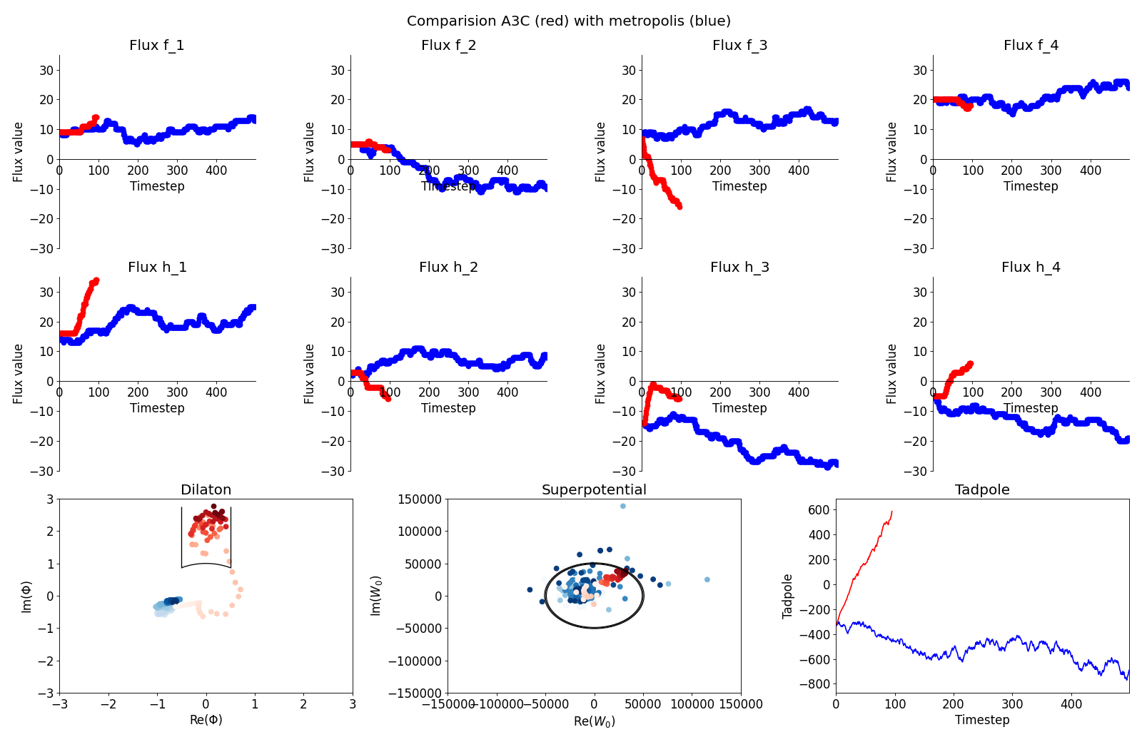
Figure 5: Here we see the result of one agent and a metropolis algorithm running through the environment. The A3C is shown in red and metropolis in blue. The plot shows the flux values they encounter as well as the dilaton and superpotential values. For the dilaton, the black line indicates the fundamental domain whereas for the superpotential the black circle defines the area of values we are looking for. The fluxes for the agent were initialized between -30 and 30. Also compared to metropolis, the A3C agent manages to find a model rather quickly and to remain inside the fundamental domain.

Both algorithms are initialized at the same flux vector and then run for up to 500 steps or until they found a good vacuum. We clearly see, that our agent first sets $h_{3}$ close to zero and then pushes $h_{1}$ and $f_{3}$ to opposite directions. This is achieved in a very fast way and hence the A3C agent finds a model way earlier then metropolis who does not succeed at all in this example. By closely inspecting the movement of the dilaton value in correspondence to the flux movements, we see that setting $h_{3}$ to zero is mainly for transitioning into the fundamental domain. We also notice, that our agent manages to almost never step outside of the domain again, whereas metropolis just walks in and out randomly. Also, our agent keeps the superpotential close to 50000 and is stepping carefully around it until he hits the desired value. Clearly this is for a specific initialization but we have observed this in several instances and note that overall the A3C finds significantly more flux vacua (cf. Figure 4).

On the torus, our agent finds order $\mathcal{O}(300)$ more models during training than metropolis and order $\mathcal{O}(1000)$ more than a random walker. The same can be found if we look at the number of steps needed to find 100 models. In this case, our trained agent needs $\sim 10^{3}$ steps while metropolis needs $\sim 3\cdot 10^{5}$ steps and a random walker needs $\sim 10^{6}$ steps. Hence A3C is again of order $\mathcal{O}(300)$ better than metropolis and of order $\mathcal{O}(1000)$ better than a random walker. We remark though, that these numbers do not hold for distinct models. The A3C only finds order $\mathcal{O}(2000)$ distinct models during training as does a metropolis algorithm. In [5] it was found, that the number of vacua is 1231, while in [34] the number scales with $0.13\leavevmode\nobreak\ L_{\text{max}}$ for $L_{\text{max}}>20$ and shrinks even more rapidly than $L^{4}$ for $L<20$. Hence, we do not expect many more vauca than the identified order $\mathcal{O}(2000)$. So our trained agent does not find more distinct models than a metropolis algorithm because there are not many more to find, but he runs towards them in a way more efficient and faster way. The shown experiments on the torus were done on a flux initialization interval of $[-3,3]$, because for a larger one like $[-30,30]$ a random walker and even a metropolis algorithm do not find any good vacua while running for $7.5\cdot 10^{6}$ steps. Therefore A3C’s learning is substantially hindered and he also does not manage to find a single model. If however, the agent trained on the interval $[-3,3]$ is run on the interval $[-30,30]$ he does find good vacua. He recognises where in the environment he is and manages to run towards small flux values where he knows all the models are. Metropolis is not able to do anything similar.

Search for $g_{s}$

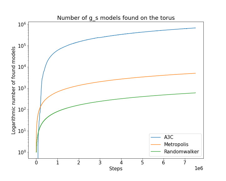
Figure 6: Plot of log number of models of A3C on the torus. He searches for string coupling values with $0.29<g_{s}<0.4$. A3C shows a good learning behaviour and outperforms the others strongly.

On the torus we also look for solutions with $0.29<g_{s}<0.4$. Since $g_{s}=\frac{1}{\text{Im}(\phi)}$ this corresponds to looking for $2.5<\text{Im}(\phi)<4$. Because we still do not want to over count and we want physically meaningful solutions, we will also imply the fundamental domain condition $|\text{Re}(\phi)|<0.5$ and the tadpole condition (10). Again, our algorithm will calculate the dilaton for all real solutions of (29). The neural network and environment structures are the same as for the superpotential search as are the hyperparameters. The distance rewards (punishments) are given by

$$r_{g} = \begin{cases}N_{g}\cdot\par\text{exp}\left(-\left(\frac{|\text{Re}(\phi)|-0.5}{\sigma_{g}}\right)^{2}\right)\ &\text{if Im}(\phi)>1\ ,\\ N_{g}\cdot\par\text{exp}\left(-\left(\frac{|\text{Re}(\phi)|-0.5}{\sigma_{g}}\right)^{2}\right)\cdot\par\par\text{exp}\left(-\left(\frac{\text{Im}(\phi)-3}{\sigma_{g}}\right)^{2}\right)\ &\text{else}\ ,\end{cases}$$ (36)

$$r_{t} = N_{t}\cdot\text{tanh}\left(\sigma_{t}\left(N_{\text{flux}}-0\right)\right)\cdot r_{\text{tad}}\ ,$$ (37)

with the constants

$$N_{g}=5\ , \quad\sigma_{g}=5\ , \quad r_{\text{gauge}}=2000\ ,$$ (38)

$$N_{t}=1\ , \quad\sigma_{t}=0.2\ , \quad r_{\text{tad}}=-5\ .$$ (39)

As RL agent, we used only the A3C since PER Duel DDQN did not succeed for the superpotential search. The agent is again compared to a random walker and a metropolis algorithm. The agent was trained for $5\cdot 10^{6}$ steps and reset after he found a model or after 500 steps. The results are plotted in Figure 6. The A3C finds significantly more solutions than the other two algorithms. To find 100 models it takes our agent again $\sim 10^{3}$ steps while metropolis needs $\sim 10^{5}$ steps and a random walker $\sim 10^{6}$. A3C is more successful because he again exploits efficiently that good vacua are to be found in a region of small flux values. More details about the torus experiments can be found in Appendix C.

To sum up, the A3C agent learns and exploits very efficiently the apparent structure in these specific environments. We did not know about this structure before, so an agent like this could be used on different and more complex environments such that he could help us there to find structures we did not know about and help us to learn more about the string landscape.
We note that prioritized dueling DDQN only manages to beat the random walker on the conifold and never beats a metropolis algorithm. We have performed an extensive hyperparameter search (see Appendix B for more details).

4 Conclusions

Understanding the landscape of flux vacua is a long-standing problem in string phenomenology. Estimates on the number of vacua require an efficient sampling technique to make progress towards understanding the landscape. We find that for few number of moduli standard metropolis explorations are already feasible to identify the correlations among different flux vacua. We found that our RL agents are able to explore a phenomenologically distinct area of flux space by providing it with an appropriate reward structure. Generally speaking, after sufficient training, the RL algorithm can outperform the metropolis explorations significantly. The main question this raises are how these methods scale with the complexity of the underlying model and whether RL algorithms remain trainable and enable in those cases significant new insights which are not attainable via metropolis sampling.

In addition we show that we are able to explore different vacua in a small region of flux space. This is crucial as the associated correlations in flux space will hold valuable information on which structures are needed for addressing the cosmological constant problem via the string landscape.

There are multiple avenues how to extend this work:

• We have restricted ourselves to vacua where analytic solutions where available. In most cases such analytic solutions are not available and one needs to search for such vacua numerically. In principle the two can be combined which will increase the runtime and potentially misses some vacua. Examples of such numerical searches can be found for instance in [20, 21].

• Do the configurations of phenomenologically interesting flux vacua reveal an interesting sub-structure which are not visible in the flux-flux correlations? It will be interesting to examine the search for such structures using topological data analysis [50, 51].

• In terms of scaling of these RL techniques, one parameter which is of interest is the initial range of flux vacua which determines roughly speaking how many vacua are nearby and whether the algorithm learns to explore a large fraction of distinct vacua or always collapses to the same ones. Our work has focused on type IIB string theory which captures only a subset of fluxes in comparison to the situation in F-theory where many more flux vacua are present where this scaling question becomes more pressing (cf. [52] for an estimate of $10^{272000}$ flux vacua on a fixed background geometry and estimates on the number of background geometries [53, 54]).

• At this moment we have to adapt our environment and reward structure for each background geometry. For a large exploration of the string landscape it seems crucial to being able to apply the same strategy across various background geometries which has the potential to reveal universal features in the identification of phenomenologically interesting vacua.

• Another approach for revealing structures is by looking at generative techniques of effective field theories satisfying certain UV [55, 56] or IR constraints [57]. Again it would be very useful to understand which methods are best suited to identify systematics in phenomenologically interesting string vacua. In particular this is to identify the best suited methods for these sparse solutions in high-dimensional spaces.

We hope to return to these questions in the future.

Appendix A RL-details

Here we provide a lightning review of the RL algorithms which we are using. Deep Q learning and its extensions are based on [43, 44, 45, 46].

A.1 Deep Q-learning

Here the state-action value function depends on the weights of a neural network

$$Q^{\pi}(s,a)\simeq Q^{\pi}_{\theta}(s,a)\ ,$$ (40)

with a state $s$, an action $a$ and the network weights $\theta$. For Deep Q-learning (DQN) one initializes two different sets of weights $\theta$ and $\theta^{\prime}$ and only updates the so called target weights $\theta^{\prime}$ after a given number of timesteps. The update rule for $\theta$ then looks like

$$\Delta\theta=\alpha(r_{t+1}+\gamma\cdot\text{max}_{a}Q^{\pi}_{\theta^{\prime}}(s_{t+1},a)-Q^{\pi}_{\theta}(s,a))\nabla_{\theta}Q^{\pi}_{\theta}(s,a)$$

with learning rate $\alpha$, reward $r_{t+1}$, discount factor $y$ and $\theta^{\prime}=\theta$ is set after a given number of timesteps. To maneuver through the environment, the agent then follows a policy

$$\pi(s)=\text{argmax}_{a}Q_{\theta}(s,a)\ ,$$ (41)

which is called a greedy policy. Following this policy is equivalent to purely exploiting. To get some exploration as well, one usually uses a so called $\epsilon$-greedy policy. Here the agent only chooses the best action with probability $1-\epsilon$ and with probability $\epsilon$ a random action. Usually one wants to explore more at the beginning of the training and chooses a start value of $\epsilon_{start}=1$ and exploit more at the end so one decreases epsilon at every time step by multiplying it with a small number like $\epsilon_{decay}=0.99985$ until a final (small) value for example $\epsilon_{\text{end}}=0.01$. The last piece we need to arrive at the commonly used DQN algorithm is experience replay. By moving through the environment the agent sees different tuples of $(s,a,r,s^{\prime})$ of state, action, reward and next state. This will lead to a trajectory in the environment represented by a series of tuples

$$\tau=((s_{0},a_{0},r_{0},s_{1}),(s_{1},a_{1},r_{1},s_{2}),\dots,(s_{T-1},a_{T-1},r_{T-1},s_{T}))\ .$$

The latest trajectories (latest $C$ tuples) will be stored in a so called replay buffer $D$. To then update the Q-function, a number $N$ of these tuples is sampled uniformly at random from the replay buffer. This avoids data inefficiency and correlation between the tuples inside one trajectory.

1:Initialize replay buffer $D$ with a fixed capacity C

2:Initialize state-action value function $Q$ with random weights $\theta$

3:Initialize target state-action value function $Q$ with weights $\theta^{\prime}=\theta$

4:Initialize $\epsilon$ to start value $\epsilon=\epsilon_{start}$

5:for episode $m=1,\cdots,M$ do

6:     Observe initial state $s_{1}$

7:     for timestep $t=1,\cdots,T$ do

8:         Select action $a_{t}=\begin{cases}\text{random action with probability }\epsilon\\ \text{argmax}_{a}Q_{\theta}(s_{t},a)\text{ otherwise}\end{cases}$

9:         Execute action $a_{t}$ in environment, observe reward $r_{t}$ and next state $s_{t+1}$ and store transition $(s_{t},a_{t},r_{t},s_{t+1})$ in $D$

10:         Sample uniformly a random minibatch of $N$ transitions $(s_{j},a_{j},r_{j},s_{j+1})$ from $D$

11:         Set $y_{j}=\begin{cases}r_{j}\text{ if episode ends at step }j+1\\ r_{j}+\gamma\text{max}_{a}Q_{\theta^{\prime}}(s_{j+1},a)\text{ otherwise}\end{cases}$

12:         Update parameters $\theta$ according to $\Delta\theta=\frac{1}{N}\sum_{j=1}^{N}\alpha(y_{j}-Q_{\theta}(s_{j},a_{j}))\nabla_{\theta}Q_{\theta}(s_{j},a_{j})$

13:         Set $\epsilon\leftarrow\text{min}(\epsilon_{end},\quad\epsilon\cdot\epsilon_{decay})$

14:         Every $X$ steps set $\theta^{\prime}=\theta$      

Algorithm 1 DQN algorithm

The whole algorithm is given in Algorithm 1.

DQN improvements

There are several performance improvements to DQN which will be covered in the following.

Double Deep Q-learning (DDQN)

DQN works in general, but suffers from the problem of overestimating values. The reason is that the target in Line 11 in Algorithm 1 is given by the maximum of the same Q function as the action is chosen from in line 8. This maximum operator comes from the idea, that the best action in the next state is given by the one with the highest Q value. But that is not necessarily the case and just an estimation. Since this estimation is done twice, once in line 8 and once in line 11, overestimation is present and the estimated values will be overoptimistic. To overcome this problem, one uses two different networks which in our case are the ones with weights $\theta$ and $\theta^{\prime}$. Then the target in line 11 for DDQN becomes

$$y^{DDQN}_{j}=r_{j}+\gamma Q_{\theta^{\prime}}\left(s_{j+1},\text{argmax}_{a}Q_{\theta}(s_{j+1},a)\right)\ .$$

The rest of the algorithm is the same as for DQN. There are further extensions to DDQN two of which will be discussed in the following.

Dueling

Dueling DQN differs from normal DQN in the network architecture. Here, before outputting the Q-function, the network will be split in two, the so called advantage function $A(s,a)=Q(s,a)-V(s)$ and the value function $V(s)$. The motivation for this is that it is not always necessary to know the value of each action choice but just the state value instead. The Q function is then again obtained by adding up the split layers and subtract the average advantage

$$Q(s,a)=V(s)+A(s,a)-\frac{1}{\mathcal{A}}\sum_{a^{\prime}}A(s,a^{\prime})\ ,$$ (42)

with $\mathcal{A}$ the dimensionality of the action space. The subtraction is needed, since otherwise $V$ and $A$ can not be recovered uniquely from the Q-function, leading to problems in backpropagation.

Prioritized experience replay

At every training step a set of states the agent has visited during training is sampled and given to the network in order to calculate and update the Q-values for these states. The idea of prioritized experience replay is to assign a probability to each state proportional to its loss and sample states according to these probabilities. In more detail, the loss of a state is given by its TD-Error

$$\delta_{i}=r_{t}+\gamma Q_{target}(s_{t+1},\text{argmax}_{a\in\mathcal{A}}Q(s_{t+1},a))-Q(s_{t},a)\ .$$

Then the so called priorities are $p_{i}=|\delta_{i}|+\epsilon$ with some small constant to ensure that the priority is never zero (which would correspond to not being sampled at all). To get to a probability, one has to norm these priorities to something between zero and one

$$P(i)=\frac{p_{i}^{\alpha}}{\sum_{k}p_{k}^{\alpha}}\ ,$$ (43)

where $k$ runs over all states. The exponents $\alpha$ determine the level of prioritization, meaning that small values lead to states being sampled more equally, whereas high values lead to a more loss dependent sampling. This method introduces an over-sampling and bias with respect to a uniform sampling. To correct for this bias by a small amount, importance sampling is used. For this purpose, one has to introduce weights

$$w_{i}=\left(\frac{1}{N}\cdot\frac{1}{P(i)}\right)^{\beta}\ ,$$ (44)

where $N$ is the buffer size meaning the number of saved states to sample from and $\beta$ is a coefficient fulfilling the same role as $\alpha$ before. These weights are multiplied by $\delta_{i}$ and then used in the gradient updates of the network

$$\Delta\theta=\alpha\leavevmode\nobreak\ w_{i}\delta_{i}\leavevmode\nobreak\ \nabla_{\theta}Q^{\pi}_{\theta}(s,a)\ .$$ (45)

This ensures, that updates coming from high probability states don’t have too much of an impact on the network parameters. The exponents are usually chosen to be $\alpha=0.1$ and $\beta=0.6$.

A.2 Asynchronous advantage actor-critic (A3C)

In actor-critic methods the policy (actor) as well as the Q-function (critic) will be approximated by a neural network

$$\pi(s,a) \simeq \pi_{\theta}(s,a)\ ,$$

$$Q(s,a) \simeq Q_{w}(s,a)\ ,$$

with the weights $\theta$ and $w$. Often, in policy approximation methods, a baseline is introduced to reduce the variance of these algorithms and hence to improve the learning behaviour. This can be done in actor-critic methods as well. The baseline will be subtracted to result in the following loss function

$$\nabla_{\theta}\text{L}(\theta)=\mathbb{E}_{\pi_{\theta}}[\nabla_{\theta}\text{log}\pi_{\theta}(s,a)(Q^{\pi_{\theta}}(s,a)-b(s))]\ .$$

One can think of this modification as a measure of how much better our approximation is than is expected by some baseline $b(s)$. Since $b(s)$ does not depend on any action, this does not change the expectation value in the equation and therefore is mathematically allowed. Choosing $b(s)=V(s)$ the value function as a baseline is particular useful and our loss is then given by

$$\nabla_{\theta}\text{L}(\theta)=\mathbb{E}_{\pi_{\theta}}[\nabla_{\theta}\text{log}\pi_{\theta}(s,a)A^{\pi_{\theta}}(s,a)]\ ,$$ (46)

with the advantage function $A^{\pi_{\theta}}=Q^{\pi_{\theta}}(s,a)-V^{\pi_{\theta}}(s)$. In a concrete implementation of this so called advantage actor-critic algorithm the value function will be approximated by a neural network since, using the TD-algorithm, the advantage function at timestep $t$ is given by $A_{w}(s_{t},a_{t})=r_{t+1}+\gamma V_{w}(s_{t+1})-V_{w}(s_{t})$. Then the critic network which approximates the value function will just be updated using $\nabla_{w}A_{w}(s,a).$ The last piece we need is the asynchronous advantage actor-critic (A3C) algorithm. Here learning and exploring is parallelized to different CPU cores. Each core has its own copy of the environment and of a global neural network. The actors then act according to their copy of the neural network and collect gradients by walking through their environment and computing the actor-critic losses. After some time (if all the different actors on the different cores would send their gradients at the same time this would be called synchronous actor-critic) an actor sends these gradients to the global network and this network is updated according to them. The actor then gets the new weights from the network and explores and computes gradients again and so on. This method has the advantages, that it allows for shorter training time due to the parallelization and for more exploration since every actor most likely explores different regions of the environment. To exploit this exploration benefit even more, the authors of [42] added an entropy regularization term to the policy loss 46

$$\nabla_{\theta}\text{L}(\theta)=\mathbb{E}_{\pi_{\theta}}[\nabla_{\theta}\text{log}\pi_{\theta}(s,a)A^{\pi_{\theta}}(s,a)+\beta\nabla_{\theta}H_{\theta}(\pi_{\theta}(s))]\ ,$$ (47)

with the entropy $H_{\theta}(\pi_{\theta}(s))=-\sum_{a}\pi_{\theta}(s,a)\text{log}\pi_{\theta}(s,a)$. Because this loss is to be maximized, the entropy will maximize as well and since the entropy measures the ”randomness” of the policy, this will lead to even more exploration.

Appendix B RL-hyperparameters

This appendix provides an overview of our hyperparameter searches we have performed. This is necessary, because the choice of hyperparameters can make the difference between a well learning and a non working agent as we will see in the case of DQN. All of the experiments shown here are done on the conifold environment with flux initialization interval $[-3,3]$. For this we will consider four value sets with different reward functions as shown in Table 1:

	$N_{s}$	$\sigma_{s}$	$r_{s}$	$\sigma_{t}$	$r_{t}$
valueset 1	$3$	$10000$	$2000$	$0.2$	$-5$
valueset 2	$5$	$50000$	$7000$	$0.2$	$-3$
valueset 3	$20$	$100000$	$10^{6}$	$0.0005$	$-3$
valueset 4	$3$	$10000$	$7000$	$0.2$	$-3$

Table 1: Different sets of reward function hyperparameters

For each valueset the other reward function hyperparameters are set as:

$$r_{g}=10,\ \sigma_{g}=2,\ N_{g}=0.5,\ N_{t}=1\ .$$ (48)

In the experiments shown in this section we will have a look at the influence of $\gamma$, which defines how much future rewards are valued compared to more short term rewards. Also, we wanted to try out different exploration rates which corresponds to $\beta$ in the case of A3C and to $\epsilon$ in the case of DQN. The value of $\epsilon$ specifies the probability, with which the agent chooses a random action. So a high $\epsilon$ means, that the agent often chooses a random action and hence explores more of the environment than he would by only following the action suggested by the neural network. On the other hand, the value of $\beta$ influences the entropy term in Equation (46) so a high value here leads to the agent paying more attention to maximising the entropy and hence leads to more exploration as well. The different values tried here are:

• A3C: $\gamma\in\{0.95,0.999,0.99999\},\ \beta\in\{0.1,0.5,1\}$

• DQN: $\gamma\in\{0.95,0.999,0.99999\},\ \epsilon\in\{0.01,0.1,0.3\}$

Each experiment trains the A3C agent for $7.5\times 10^{6}$ steps and the DQN agent for $15\times 10^{6}$ steps. The agent is reset every 500 steps or if he found a good vacuum. The results are always given in terms of the number of good vacua the agent found during training. Results for the A3C experiments are given on the left side in Figure 7.

Figure 7: Results of hyperparameter scan for different reward functions for A3C (left) and DQN (right) experiments.

In all experiments, a small $\gamma$ value performs best. That means it is more beneficial for the agent to prefer short term rewards, so just increasing the distance reward step by step instead of focusing on hitting a good vacuum somewhere in the future. On the other hand the $\beta$ value does not have as much of an impact. A higher value there leads to a faster learning. However, the small $\beta$ always catches up and for valueset 1 and 3 even beats the others. So we conclude, that a higher $\beta$ which corresponds to more exploration, leads to a faster but less successful learning. Concerning the valueset, in all three cases the agent finds around 150000 not necessarily distinct models. However, valueset 3 gives the highest amount and hence we choose to work with that one. So our best working agent uses valueset 3 with hyperparameters $\gamma=0.95$ and $\beta=0.1$. In all cases the metropolis algorithm finds order $\mathcal{O}(20)$ less models then our agent, while a random walker finds order $\mathcal{O}(600)$ less.
Next, the results for the DQN experiments are given on the right side in Figure 7. The first thing to note is, that a high $\gamma$ performs worst again. Different to A3C though it is the middle value for $\gamma=0.999$ that works best. Concerning the exploration parameter $\epsilon$, the performance seems to depend on the valueset. For valuesets 1 and 2 a higher $\epsilon$ and hence taking a random action more often works better. For valuesets 3 and 4 however exploiting works best. If we now focus on the total number of found models, we see that not a single agent beats metropolis and only for valueset 1 and 4 some manage to beat a random walker. Also, the slope of the model curve does only change for valueset 4 and hence only there some kind of learning behaviour is present. The best agent for valueset 1 finds roughly 800 models while for valueset 4 he finds 700. In both cases that is a factor of 1.5 more then for a random walker. However, metropolis finds $\mathcal{O}(20)$ more. All of these insights are for the models found during training. If we look at some evaluation runs of trained agents and compare those to metropolis and a random walker, the results are given in Figure 9. There we see, that only for valueset 4, the agent manages to beat metropolis by a factor of 2. Hence we choose valueset 4 as our best working reward function for DQN.

Figure 8: Results of 500000 evaluation steps for the DQN agents valuesets 1 and 4 and comparison to a random walker and metropolis.

Figure 9: Comparison of DQN to its extensions: PER Duel DDQN outperforms the single extensions strongly.

Figure 10: Logarithmic number of found models for A3C experiments with different model complexities.

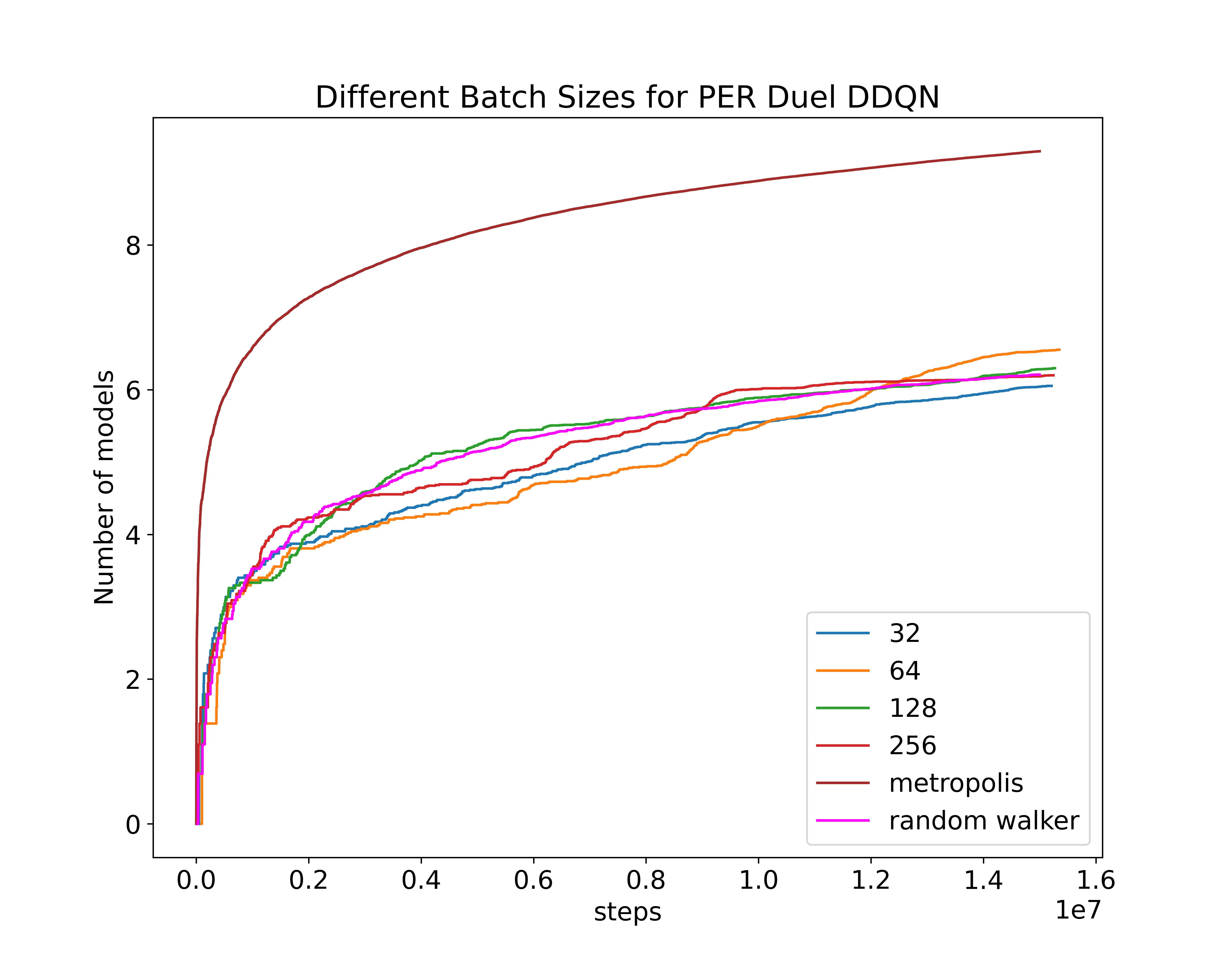
Figure 11: Logarithmic number of found models for DQN experiments with different batch sizes.

Model complexity

Here we want to study the influence of different neural network architectures. For that purpose, we will look at an A3C agent with optimal hyperparameters and valueset, i.e. $\gamma=0.95$, $\beta=0.1$ and valueset 3 respectively. The network will always be dense and consist of 4 hidden layers. However, the size of these layers will be varied in the following way:

Layer number	1	2	3	4
Layer size	50	50	50	50
	50	200	50	50
	50	50	200	50
	50	50	50	200
	1000	1000	1000	1000

Table 2: Different sets of reward function hyperparameters.

Also, we tried to include dropouts with probability $p=0.5$. In all these experiments the agent was run for $7.5\cdot 10^{6}$ steps or 120 hours whatever occurred first. The results in terms of logarithmic number of found models is shown in Figure 11. First, we notice that the run with layer size 1000 was stopped early since it reached the 120 hours time mark. So even if it might perform better at late times, it is not suitable for our purpose. Dropout does not perform well either. All other architectures do not differ much to each other, but the red curve reaches the most models and an equally fast learning behaviour, so we choose to work with that one. We did not try convolutional architectures since our problem is not translation invariant.

Batch size

Next we study the influence of the batch size on the DQN agent Figure 11. As we can see, only for batch size 64 the curve gets steeper at around $9\cdot 10^{6}$ steps and hence only there the agent shows some learning behaviour. Therefore we choose to work with that batch size.

DQN variants

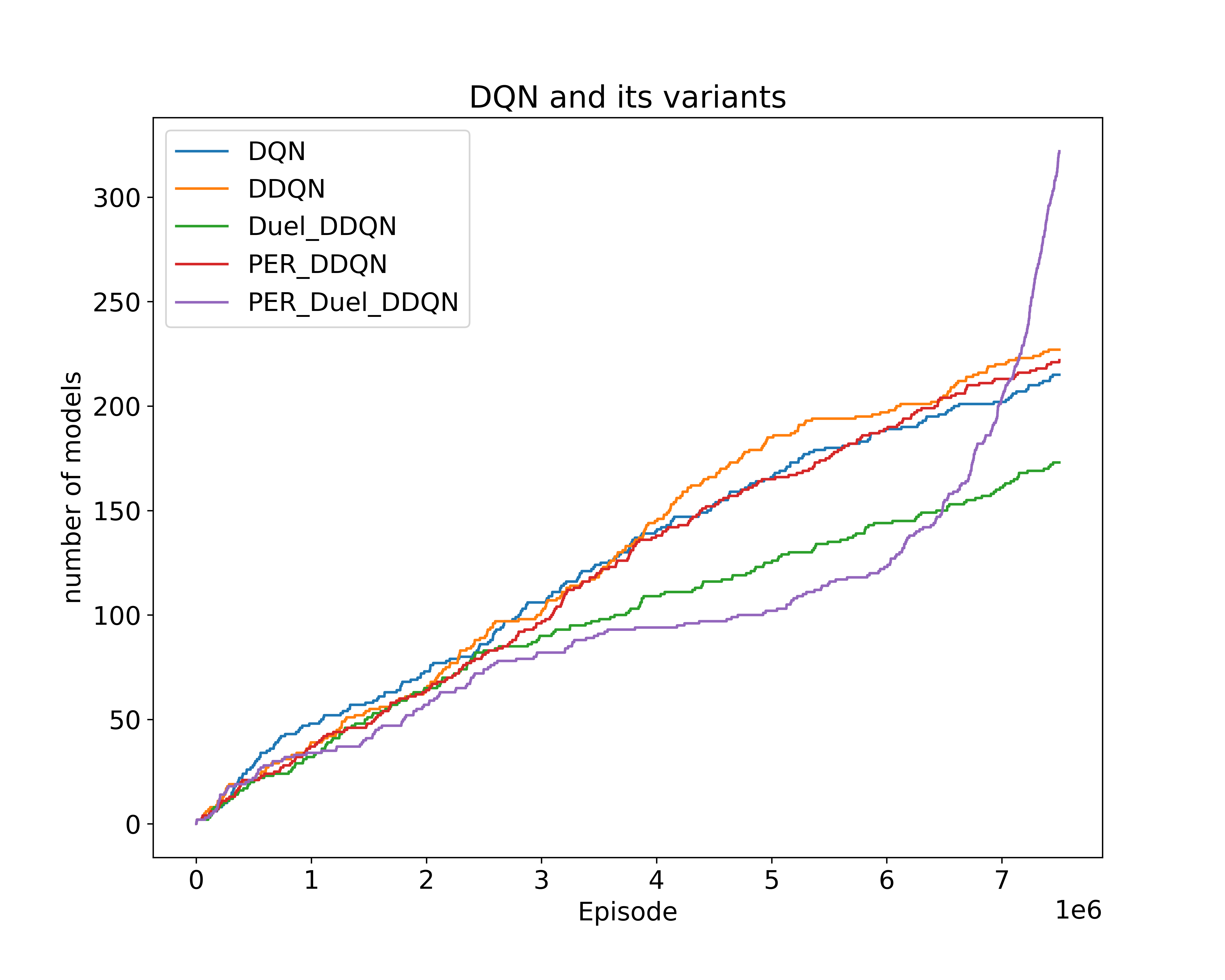
Figure 12: Comparison of DQN to its extensions: PER Duel DDQN contains all other shown extensions to DQN and adds prioritized experience replay. Hence, it outperforms the single extensions strongly.

The next plot Figure 12 shows the comparison of DQN to its different extensions. All hyperparameters are put to default values and valueset 4 was used. The agents were trained for $7.5\cdot 10^{6}$ steps and reset after they found a model or 500 steps. One can see, that PER Dueling DDQN performs best. The same holds for the comparison on the level of evaluation Figure 9. The reason for this might be the nature of prioritized experience replay. Since in our environment, states fulfilling all of our conditions are rare, the agent won’t see them very often during training and hence can not learn much from them. Due to PER though, they can be sampled more often leading to a better performance.

Appendix C Torus environment

In this appendix, we will present more details about our experiments on the torus. We looked for specific values of the superpotential $|W_{0}|$ and the string coupling $g_{s}$.

Superpotential search

Here we will look for solutions with $0<|W_{0}|<10$. Of course the dilaton (12) and tadpole condition (10) also have to be satisfied. Our algorithm will calculate the dilaton for all real solutions of Equation (29). The superpotantial then will only be calculated for the values of $\tau$ for which the dilaton lies in the fundamental domain. The structure of the environment are the same as in chapter 3. The neural network contains again 4 dense layers with 50 neurons for the first three and 200 for the last layer. The distance rewards (punishments) are given by

$$r_{g} = \begin{cases}N_{g}\cdot\par\text{exp}\left(-\left(\frac{|\text{Re}(\phi)|-0.5}{\sigma_{g}}\right)^{2}\right)\cdot r_{\rm gauge}\ &\text{if Im}(\phi)>1\ ,\\ N_{g}\cdot\par\text{exp}\left(-\left(\frac{|\text{Re}(\phi)|-0.5}{\sigma_{g}}\right)^{2}\right)\cdot\par\par\text{exp}\left(-\left(\frac{\text{Im}(\phi)-1}{\sigma_{g}}\right)^{2}\right)\cdot r_{\rm gauge}\ &\text{else}\ ,\end{cases}$$ (49)

$$r_{t} = \begin{cases}N_{t}\cdot\text{tanh}\left(\sigma_{t_{1}}\left(N_{\text{flux}}-0\right)\right)\cdot r_{\text{tad}}\ \text{if}\ N_{\text{flux}}<0\ ,\\ N_{t}\cdot\text{tanh}\left(\sigma_{t_{2}}\left(N_{\text{flux}}-0\right)\right)\cdot r_{\text{tad}}\ \text{if}\ N_{\text{flux}}>16\ ,\end{cases}$$ (50)

$$r_{s} = N_{s}\cdot\text{exp}\left(-\left(\frac{|W_{0}|-0}{\sigma_{s}}\right)^{2}\right)\ ,$$ (51)

with the constants

$$N_{g}=0.5\ , \quad\sigma_{g}=2\ , \quad r_{\text{gauge}}=10\ ,$$ (52)

$$N_{t}=1\ , \quad\sigma_{t_{1}}=0.003\ , \quad\sigma_{t_{2}}=0.0005\ ,\quad r_{\text{tad}}=-5$$ (53)

$$N_{s}=20\ , \quad\sigma_{s}=3000\ , \quad r_{\text{sup}}=100000\ .$$ (54)

As RL agent, we used the best two from the conifold experiments, namely an A3C and a prioritized experience replay duel DDQN. They are again compared to a random walker and a metropolis algorithm. The hyperparameters are chosen the same way as for the conifold. The agent was trained for $7.5\cdot 10^{6}$ steps and reset after he found a model or after 500 steps.

References

- [1] R. Bousso and J. Polchinski, Quantization of four-form fluxes and dynamical neutralization of the cosmological constant, Journal of High Energy Physics 2000 (Jun, 2000) 006–006.
- [2] L. Susskind, The Anthropic landscape of string theory, hep-th/0302219.
- [3] M. R. Douglas, The statistics of string/m theory vacua, Journal of High Energy Physics 2003 (May, 2003) 046–046.
- [4] S. K. Ashok and M. R. Douglas, Counting flux vacua, Journal of High Energy Physics 2004 (Jan, 2004) 060–060.
- [5] F. Denef and M. R. Douglas, Distributions of flux vacua, Journal of High Energy Physics 2004 (May, 2004) 072–072.
- [6] M. R. Douglas, B. Shiffman, and S. Zelditch, Critical points and supersymmetric vacua i, Communications in Mathematical Physics 252 (Oct, 2004) 325–358.
- [7] N. Arkani-Hamed, S. Dimopoulos, and S. Kachru, Predictive landscapes and new physics at a TeV, hep-th/0501082.
- [8] F. Denef and M. R. Douglas, Distributions of nonsupersymmetric flux vacua, Journal of High Energy Physics 2005 (Mar, 2005) 061–061.
- [9] L. SUSSKIND, Supersymmetry breaking in the anthropic landscape, From Fields to Strings: Circumnavigating Theoretical Physics (Feb, 2005) 1745–1749.
- [10] M. Dine, E. Gorbatov, and S. Thomas, Low energy supersymmetry from the landscape, Journal of High Energy Physics 2008 (Aug, 2008) 098–098.
- [11] J. P. Conlon and F. Quevedo, On the explicit construction and statistics of calabi-yau flux vacua, Journal of High Energy Physics 2004 (Oct, 2004) 039–039.
- [12] R. Kallosh and A. Linde, Landscape, the scale of susy breaking, and inflation, Journal of High Energy Physics 2004 (Dec, 2004) 004–004.
- [13] F. Marchesano, G. Shiu, and L.-T. Wang, Model building and phenomenology of flux-induced supersymmetry breaking on d3-branes, Nuclear Physics B 712 (Apr, 2005) 20–58.
- [14] M. Dine, D. O’Neil, and Z. Sun, Branches of the landscape, Journal of High Energy Physics 2005 (Jul, 2005) 014–014.
- [15] B. S. Acharya, F. Denef, and R. Valandro, Statistics ofmtheory vacua, Journal of High Energy Physics 2005 (Jun, 2005) 056–056.
- [16] K. R. Dienes, Statistics on the heterotic landscape: Gauge groups and cosmological constants of four-dimensional heterotic strings, Physical Review D 73 (May, 2006).
- [17] F. Gmeiner, R. Blumenhagen, G. Honecker, D. Lüst, and T. Weigand, One in a billion: Mssm-like d-brane statistics, Journal of High Energy Physics 2006 (Jan, 2006) 004–004.
- [18] M. R. Douglas and W. Taylor, The landscape of intersecting brane models, Journal of High Energy Physics 2007 (Jan, 2007) 031–031.
- [19] Y. Sumitomo and S. H. H. Tye, A Stringy Mechanism for A Small Cosmological Constant, JCAP 08 (2012) 032, [arXiv:1204.5177].
- [20] D. Martinez-Pedrera, D. Mehta, M. Rummel, and A. Westphal, Finding all flux vacua in an explicit example, JHEP 06 (2013) 110, [arXiv:1212.4530].
- [21] M. Cicoli, D. Klevers, S. Krippendorf, C. Mayrhofer, F. Quevedo, and R. Valandro, Explicit de Sitter Flux Vacua for Global String Models with Chiral Matter, JHEP 05 (2014) 001, [arXiv:1312.0014].
- [22] I. Broeckel, M. Cicoli, A. Maharana, K. Singh, and K. Sinha, Moduli Stabilisation and the Statistics of SUSY Breaking in the Landscape, JHEP 10 (2020) 015, [arXiv:2007.0432].
- [23] I. Broeckel, M. Cicoli, A. Maharana, K. Singh, and K. Sinha, Moduli Stabilisation and the Statistics of Axion Physics in the Landscape, arXiv:2105.0288.
- [24] F. Denef and M. R. Douglas, Computational complexity of the landscape. I., Annals Phys. 322 (2007) 1096–1142, [hep-th/0602072].
- [25] F. Denef, M. R. Douglas, B. Greene, and C. Zukowski, Computational complexity of the landscape II—Cosmological considerations, Annals Phys. 392 (2018) 93–127, [arXiv:1706.0643].
- [26] J. Halverson and F. Ruehle, Computational Complexity of Vacua and Near-Vacua in Field and String Theory, Phys. Rev. D 99 (2019), no. 4 046015, [arXiv:1809.0827].
- [27] N. Bao, R. Bousso, S. Jordan, and B. Lackey, Fast optimization algorithms and the cosmological constant, Phys. Rev. D 96 (2017), no. 10 103512, [arXiv:1706.0850].
- [28] F. Ruehle, Data science applications to string theory, Phys. Rept. 839 (2020) 1–117.
- [29] R. S. Sutton and A. G. Barto, Reinforcement Learning: An Introduction. The MIT Press, second ed., 2018.
- [30] J. Halverson, B. Nelson, and F. Ruehle, Branes with brains: exploring string vacua with deep reinforcement learning, Journal of High Energy Physics 2019 (Jun, 2019).
- [31] M. Larfors and R. Schneider, Explore and Exploit with Heterotic Line Bundle Models, Fortsch. Phys. 68 (2020), no. 5 2000034, [arXiv:2003.0481].
- [32] T. R. Harvey and A. Lukas, Particle Physics Model Building with Reinforcement Learning, arXiv:2103.0475.
- [33] A. Cole, A. Schachner, and G. Shiu, Searching the Landscape of Flux Vacua with Genetic Algorithms, JHEP 11 (2019) 045, [arXiv:1907.1007].
- [34] O. DeWolfe, A. Giryavets, S. Kachru, and W. Taylor, Enumerating flux vacua with enhanced symmetries, Journal of High Energy Physics 2005 (Feb, 2005) 037–037.
- [35] M. R. Douglas and S. Kachru, Flux compactification, Reviews of Modern Physics 79 (May, 2007) 733–796.
- [36] L. E. Ibanez and A. M. Uranga, String theory and particle physics: An introduction to string phenomenology. Cambridge University Press, 2, 2012.
- [37] S. Gukov, C. Vafa, and E. Witten, CFT’s from Calabi-Yau four folds, Nucl. Phys. B 584 (2000) 69–108, [hep-th/9906070]. [Erratum: Nucl.Phys.B 608, 477–478 (2001)].
- [38] A. Giryavets, S. Kachru, P. K. Tripathy, and S. P. Trivedi, Flux compactifications on Calabi-Yau threefolds, JHEP 04 (2004) 003, [hep-th/0312104].
- [39] A. Giryavets, S. Kachru, and P. K. Tripathy, On the taxonomy of flux vacua, JHEP 08 (2004) 002, [hep-th/0404243].
- [40] V. Balasubramanian, P. Berglund, J. P. Conlon, and F. Quevedo, Systematics of moduli stabilisation in Calabi-Yau flux compactifications, JHEP 03 (2005) 007, [hep-th/0502058].
- [41] G. Brockman, V. Cheung, L. Pettersson, J. Schneider, J. Schulman, J. Tang, and W. Zaremba, Openai gym, CoRR abs/1606.01540 (2016) [arXiv:1606.0154].
- [42] V. Mnih, A. P. Badia, M. Mirza, A. Graves, T. P. Lillicrap, T. Harley, D. Silver, and K. Kavukcuoglu, Asynchronous methods for deep reinforcement learning, 2016.
- [43] V. Mnih, K. Kavukcuoglu, D. Silver, A. Rusu, J. Veness, M. Bellemare, A. Graves, M. Riedmiller, A. Fidjeland, G. Ostrovski, S. Petersen, C. Beattie, A. Sadik, I. Antonoglou, H. King, D. Kumaran, D. Wierstra, S. Legg, and D. Hassabis, Human-level control through deep reinforcement learning, Nature 518 (02, 2015) 529–33.
- [44] Z. Wang, T. Schaul, M. Hessel, H. van Hasselt, M. Lanctot, and N. de Freitas, Dueling network architectures for deep reinforcement learning, 2016.
- [45] T. Schaul, J. Quan, I. Antonoglou, and D. Silver, Prioritized experience replay, 2016.
- [46] H. van Hasselt, A. Guez, and D. Silver, Deep reinforcement learning with double q-learning, 2015.
- [47] S. Tokui, K. Oono, S. Hido, and J. Clayton, Chainer: a next-generation open source framework for deep learning, in Proceedings of Workshop on Machine Learning Systems (LearningSys) in The Twenty-ninth Annual Conference on Neural Information Processing Systems (NIPS), 2015.
- [48] A. Paszke, S. Gross, F. Massa, A. Lerer, J. Bradbury, G. Chanan, T. Killeen, Z. Lin, N. Gimelshein, L. Antiga, A. Desmaison, A. Köpf, E. Yang, Z. DeVito, M. Raison, A. Tejani, S. Chilamkurthy, B. Steiner, L. Fang, J. Bai, and S. Chintala, Pytorch: An imperative style, high-performance deep learning library, 2019.
- [49] W. Lerche, D. Lust, and A. N. Schellekens, Chiral Four-Dimensional Heterotic Strings from Selfdual Lattices, Nucl. Phys. B 287 (1987) 477.
- [50] M. Cirafici, Persistent Homology and String Vacua, JHEP 03 (2016) 045, [arXiv:1512.0117].
- [51] A. Cole and G. Shiu, Topological Data Analysis for the String Landscape, JHEP 03 (2019) 054, [arXiv:1812.0696].
- [52] W. Taylor and Y.-N. Wang, The F-theory geometry with most flux vacua, JHEP 12 (2015) 164, [arXiv:1511.0320].
- [53] J. Halverson, C. Long, and B. Sung, Algorithmic universality in F-theory compactifications, Phys. Rev. D 96 (2017), no. 12 126006, [arXiv:1706.0229].
- [54] W. Taylor and Y.-N. Wang, Scanning the skeleton of the 4D F-theory landscape, JHEP 01 (2018) 111, [arXiv:1710.1123].
- [55] H. Erbin and S. Krippendorf, GANs for generating EFT models, Phys. Lett. B 810 (2020) 135798, [arXiv:1809.0261].
- [56] J. Halverson and C. Long, Statistical Predictions in String Theory and Deep Generative Models, Fortsch. Phys. 68 (2020), no. 5 2000005, [arXiv:2001.0055].
- [57] J. Hollingsworth, M. Ratz, P. Tanedo, and D. Whiteson, Efficient sampling of constrained high-dimensional theoretical spaces with machine learning, arXiv:2103.0695.