Supplementary information
A Long Short-Term Memory for AI Applications in Spike-based Neuromorphic Hardware

S1 Neuron models

S1.1 Neuron Parameters

The parameters pertaining to the neurons used in the AHP-SNNs are listed in Table S1.

			Spiking RelNet
Parameter		sMNIST	Original	Stretched in time
Neuron Parameters:
	PSC decay $\tau_{I}$ (steps)	0.0	7.0	20.0
	Voltage decay $\tau_{V}$ (steps)	20.0	7.0	20.0
	AHP-current decay $\tau_{AHP}$ (steps)	700.0	40.3	120.0
	AHP-current decrement $\beta$ / $V_{\text{thr}}$	0.756	0.176	0.062
	Refractory period $\tau_{ref}$	0	0	2
Surrogate gradient Parameters:
	Dampening factor $\gamma$	0.3	0.0	0.5
	Scaled voltage support $\left[v_{-},v_{+}\right]$	$\left[-1.0,1.0\right]$	$\left[-1.0,0.5\right]$	$\left[-1.0,0.5\right]$

Table S1: LIF-neuron and AHP-neuron parameters:  Here we detail the parameters for the spiking neurons used in the different examples. In each task, the parameters for the AHP-neurons are identical to those of the LIF-neurons, with the exception of the additional parameters $\beta$ and $\tau_{AHP}$. The examples for which the parameters are shown are: the sMNIST task solved by a single AHP-SNN network, the "original" version of the Spiking RelNet on the bAbI task that is benchmarked in the main text, and a Spiking RelNet where all parameters are adjusted to effectively slow the simulation down, and increase temporal resolution by a factor of 3 (for which the results are shown in Table S3)

S2 Energy and Time benchmarking

In order to evaluate the energy efficiency of our spiking networks implemented on the neuromorphic chip Loihi from Intel [Davies et al., 2018] we measured the energy and latency of a task and compared it with the artificial neuronal network implementation on conventional hardware, i.e., CPUs and GPUs.

For the network executed on a Loihi system the performance is measured by reading out sensors of the hardware. Regarding the energy measurement, Loihi chips of a system are powered by on-board voltage regulators that support power telemetry over an I²C interface. These voltage regulators are used to collect power usage information. In particular, the SDK of Loihi allows to split the contributions of static and dynamic power consumption as well as estimate the contribution of neuro-cores and on-chip synchronous x86 cores to the overall power consumption.

For Energy measurement on CPU the Intel Power Gadget 3.5, a software based power estimation tool, was used. For GPUs we used the nvidia-smi tool to measure the power, which is also a software based estimation tool. The nvidia-smi tool does not give a detailed breakdown of where power is consumed, but rather report the power draw of the whole board. Therefore we measured a baseline idle power draw, which we considered for the static energy. Afterwards we measure the power consumption during the workload, which denotes to the total energy and then we calculated the dynamic energy by subtracting the static energy from the total energy.

For both Loihi and CPU/GPU the measurements were performed for a workload running long enough to get in a steady state for power draw. Therefore, the batch size 50 and 100 examples on the GPU required us to run the test set several times to achieve a steady state. The execution time for networks executed on Loihi and networks running on CPU or GPU was measured on python level using the timeit module and can be considered a wall-clock time. This wall-clock time is then divided by the number of samples used for inference to calculate the latency. The execution time was measured independent of the power measurements.

S3 Details for AHP-SNN on the sMNIST task

S3.1 Input encoding for sMNIST

In Listing S1 the pseudo code for the input encoding used in the sMNIST task is shown. We assume that the current pixel value and next pixel value of the input image are presented, the number of thresholds were chosen to be half of the input neurons and thresholds are linearly spaced between 0 and 255 (number of threshold times).

⬇

while threshold_counter <= num_thresholds:

thr = thresholds[threshold_counter]

# transition from a lower pixel value to a higher pixel value

if current_pixel_value <= thr and next_pixel_value >= thr:

input neuron with the id 2*threshold_counter spikes

# transition from a higher pixel value to a lower pixel value

if current_pixel_value >= thr and next_pixel_value <= thr:

input neuron with the id (2*threshold_counter + 1) spikes

threshold_counter += 1

Listing S1: Input encoding sMNIST. Pseudo code for the input spike encoding of MNIST images used in the sMNIST task.

S3.2 Energy and latency benchmarking results

The detailed benchmarking results for the ASP-SNN solving the sMNIST task on Loihi are given in Table 1. Here we compare the energy consumed, the latency (also called delay) to compute the output, and the resultant energy-delay product with an implementation of an LSTM running on a GPU.

Power (mW) Time per Latency Latency Energy per Energy Energy Delay EDP Hardware # cores Static Dynamic Total time step (µs) (ms) ratio Inference (mJ) ratio Product (µJs) ratio Loihi 1 x86 cores 0.08 24.33 24.41 16.79 14.11 1.00x 0.34 1.00x 5.14 1.00x neuron cores 0.51 0.91 1.42 0.02 total 0.59 25.24 25.83 0.36 Nvidia RTX 2070 - batch size 1 33898.00 34602.00 68500.00 - 39.73 2.82x 2721.51 7,467.20x 108125.39 21,025.64x batch size 50 33898.00 38171.00 72069.00 - 37.44 2.65x 53.97 148.07x 2020.46 392.89x batch size 100 33898.00 53287.00 87185.00 - 40.41 2.86x 35.23 96.67x 1423.70 276.85x Intel Core i5-7440HQ - batch size 1 2040.00 18886.00 20926.00 - 83.15 5.89x 1740.00 4,774.16x 144680.74 28,134.05x

Table S2: Benchmark results for sMNIST: Comparison of energy and time measurements of the spiking AHP-SNN network on Loihi against the corresponding LSTM on GPU and CPU solving the sMNIST task.

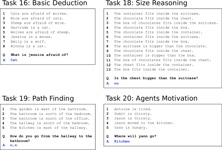
Figure S1: Examples for four types of tasks in the bAbI dataset:  Each example consists of a story and a question which allows a single word answer (except for Task 19, where two directions can be given as answer). The dataset consists of 20 types of tasks, each targeting a different aspect of reasoning. In this figure, examples from four tasks are shown. Each one demonstrates the requirement for relational reasoning in order to successfully answer the question. “Basic Deduction”, “Path Finding”, and “Size Reasoning” require only reasoning across multiple sentences. Task 20 “Agents Motivation” requires in addition association of concepts with information that is external to the current story.

S4 Details for the Spiking RelNet on the bAbI task

S4.1 Output accuracy of the Spiking RelNet

The Spiking RelNet is trained on the combined data from 17 out of 20 bAbI tasks and it’s performance is compared to an implementation of a non-spiking RelNet in Table S3. We have excluded the 3 tasks "Task 2: Two Supporting Facts", "Task 3: Three Supporting Facts", and "Task 16: Basic Induction". For an example of some of the tasks on which the network was trained, see Fig. S1. This is because the non-spiking RelNet did not converge on these tasks. The network we trained was able to solve 16/17 tasks to within a 5% Error, which is the threshold at which a task is considered solved (used in [Santoro et al., 2017], and [Weston et al., 2015]).

The task "Task 17: Positional Reasoning" has a rather high error, which we think is because the comparatively complex sentences in this task require a longer compute time to process. This is a trade-off we make for faster training and energy efficiency. With a larger number of time steps we find that Task 17 can in-fact be solved. To evidence this, we show two additional columns in Table S3.

The first column corresponds to a case where we simply extend the number of time steps for which we run the feed-forward part of the Spiking RelNet. Here we pad the embeddings upto a longer $T_{sim}=45\,\mbox{ms}$ (compared to $T_{sim}=37\,\mbox{ms}$ as specified in the Methods of the main text), and run the feed-forward part of the relational network (i.e. modules C–E in main text Fig. 4) for these many time steps. We observe here that while Task 17 is not yet under $5\%$ error, the error has dropped significantly.

The second column shows a simulation where all the time constants, refractory periods, $T_{inp}$, $T_{sim}$, and time per word in embedding are tripled. The parameters are additionally adjusted so that the simulation is effectively slowed by a factor of 3. The resulting time lengths used are $T_{inp}=40\,\mbox{ms}$, $T_{sim}=110\,\mbox{ms}$, $T_{\text{word}}=30\,\mbox{ms}$. The tripled time constants are provided in table S1. We see here that the additional temporal resolution allows all 17 tasks to be solved within $5\%$ classification error. However, with the 3-fold increase in time, we get a 4.5-fold (from 148.47 to 663.80) increase in the energy-delay product. Roughly the same number of total spikes are used in both cases,

This result demonstrates that it is possible to gain a significant gain in energy efficiency with a slight decrease in the overall performance (only a single task suffers loss in performance) in the bAbI task.

Task Name Spiking Non-spiking Spiking RelNet with RelNet RelNet increased compute time $T_{sim}=37$ steps $T_{sim}=45$ steps Stretched in time: all times, time constants and refractory period tripled Task 1: Single Supporting Fact 1.0 0.4 0.6 1.0 Task 2: Two Supporting Facts – 20.8 – – Task 3: Three Supporting Facts – 25.0 – – Task 4: Two Argument Relations 0.1 0.0 0.0 0.1 Task 5: Three Argument Relations 2.3 0.6 1.2 2.3 Task 6: Yes/No Questions 0.2 0.0 0.3 0.4 Task 7: Counting 0.7 0.6 0.6 1.4 Task 8: Lists/Sets 0.5 0.1 0.3 0.9 Task 9: Simple Negation 0.1 0.1 0.1 0.7 Task 10: Indefinite Knowledge 2.3 1.8 1.5 1.7 Task 11: Basic Coreference 0.9 1.5 1.6 2.1 Task 12: Conjunction 4.8 3.6 4.3 4.2 Task 13: Compound Coreference 3.9 2.5 3.6 3.6 Task 14: Time Reasoning 0.9 0.7 0.5 0.0 Task 15: Basic Deduction 0.1 0.0 0.0 0.0 Task 16: Basic Induction – 52.6 – – Task 17: Positional Reasoning 18.4 4.6 6.5 2.3 Task 18: Size Reasoning 1.5 0.6 0.8 0.2 Task 19: Path Finding 0.8 7.9 1.5 3.7 Task 20: Agent Motivations 0.0 0.0 0.0 0.4

Table S3: Percentage error of different architectures on the different tasks of the bAbI dataset:   According to Weston et al. [Weston et al., 2015], tasks with errors under 5% are considered solved. The four columns from left-to-right are as follows. Column 1:  Error of the Spiking RelNet (version benchmarked in the main text) on the 17 tasks it was trained on. All but task 17 are solved to within 5% Error. Column 2:  Error of the non-spiking RelNet (our implementation) on the 20 tasks it was trained on. Column 3:  Spiking RelNet where we increase just the number of compute steps of the feed-forward networks to $T_{sim}=45\,\mbox{ms}$ (compared to $37\,\mbox{ms}$ in the original network). We see here an immediate improvement in the performance of task 17. Column 4:  Spiking RelNet with all time lengths, refractory periods, and time constants tripled compared to the original network, and other parameters adjusted to effectively slow the entire simulation by a factor of three. We now have $T_{sim}=110\,\mbox{ms}$, $T_{inp}=40\,\mbox{ms}$, $T_{\text{word}}=30\,\mbox{ms}$ (compared to $T_{sim}=37\,\mbox{ms}$, $T_{inp}=14\,\mbox{ms}$, $T_{\text{word}}=10\,\mbox{ms}$ in the original network). Other parameters are compared in Table S1. With all times tripled, we can solve all 17 tasks to under 5% error. However, when implemented, the EDP increases roughly 4.5-fold. Thus we see that we tradeoff accuracy on a single task for a significant improvement in energy efficiency

S4.2 Energy and latency benchmarking results for the Spiking RelNet

The detailed benchmarking results of the Spiking RelNet applied to the bAbI dataset are shown in Table 2, where we compare the Spiking RelNet on Loihi to a non-spiking RelNet on a GPU in terms of the energy consumed, the latency (also called delay) in the calculation of the output, and the energy-delay product. We also show there how this varies with task size.

# sentences Power (W) Time per Latency Latency Energy per Energy Energy Delay EDP Hardware # cores Static Dynamic Total time step (µs) (ms) ratio Inference (mJ) ratio Product (µJs) ratio Loihi 20 2320 cores x86 cores 0.01 0.44 0.44 45.73 6.54 1.00x 2.89 1.00x 148.47 1.00x neuron cores 1.89 1.14 3.03 19.82 total 1.90 1.57 3.47 22.70 Nvidia RTX 2070 20 batch size 1 33.50 5.89 39.39 - 2.51 0.38x 98.88 4.36x 248.18 1.67x batch size 50 33.50 73.86 107.36 - 4.43 0.68x 9.51 0.42x 42.14 0.28x batch size 100 33.50 82.38 115.88 - 8.26 1.26x 9.57 0.42x 79.06 0.53x Loihi 16* 1552 cores x86 cores 0.00 0.43 0.43 55.89 7.99 1.00x 3.47 1.00x 151.77 1.00x neuron cores 1.16 0.78 1.94 15.52 total 1.17 1.21 2.38 18.99 Nvidia RTX 2070 16 batch size 1 33.36 5.47 38.82 - 2.6 0.33x 100.94 5.32x 262.45 1.73x batch size 50 33.36 51.47 84.83 - 4.82 0.60x 8.18 0.43x 39.42 0.26x batch size 100 33.36 76.36 109.71 - 5.43 0.68x 5.96 0.31x 32.35 0.21x Loihi 10 700 cores x86 cores 0.01 0.44 0.45 36.36 5.20 1.00x 2.33 1.00x 58.73 1.00x neuron cores 0.86 0.86 1.72 8.96 total 0.87 1.30 2.17 11.30 Nvidia RTX 2070 10 batch size 1 33.90 4.63 38.53 - 2.28 0.44x 87.86 7.78x 200.31 3.41x batch size 50 33.90 54.37 88.27 - 3.47 0.67x 6.13 0.54x 21.26 0.36x batch size 100 33.90 65.15 99.05 - 3.97 0.76x 3.93 0.35x 15.61 0.27x Loihi 6 332 cores x86 cores 0.01 0.45 0.46 27.64 3.95 1.00x 1.81 1.00x 29.11 1.00x neuron cores 0.42 0.99 1.41 5.56 total 0.43 1.44 1.86 7.37 Nvidia RTX 2070 6 batch size 1 33.80 5.58 39.38 - 2.23 0.56x 87.82 11.92x 195.84 6.73x batch size 50 33.80 44.76 78.56 - 3.2 0.81x 5.03 0.68x 16.09 0.55x batch size 100 33.80 52.82 86.62 - 3.76 0.95x 3.26 0.44x 12.25 0.42x Loihi 2 124 cores x86 cores 0.01 0.46 0.47 22.96 3.28 1.00x 1.53 1.00x 18.36 1.00x neuron cores 0.17 1.07 1.24 4.06 total 0.18 1.53 1.70 5.59 Nvidia RTX 2070 2 batch size 1 33.27 4.99 38.26 - 2.41 0.73x 92.20 16.49x 222.21 12.10x batch size 50 33.27 41.62 74.89 - 2.92 0.89x 4.37 0.78x 12.77 0.70x batch size 100 33.27 46.38 79.64 - 3.48 1.06x 2.77 0.50x 9.64 0.53x

Table S4: Benchmark results for question-answering task using RelNet Benchmarking comparison and scaling analysis of the Spiking RelNet on Loihi against the corresponding ANN on GPU. The data set was grouped by number sentences per sample which in turn determines the number of AHP-SNNs and therefore cores per sample. Measurements were done using 250 input samples. The energy per inference was calculated using total power values.
*For network size 16 only 100 input samples were used, as there are not enough test samples containing 16 sentences.

S4.3 Details of the Spiking RelNet architecture

The embedding networks

In order to embed sentences and questions into spike sequence, we use AHP-SNN Networks. The AHP-SNN network for sentences uses a different set of weights than those used by the AHP-SNN network for questions, however all other parameters are identical and are described below.

Each AHP-SNN contains $100$ LIF-neurons and $100$ AHP-neurons. The synaptic delays take an integer value uniformly from 1 to 3 ms. Note here that all time lengths and time constants are specified in terms of computation steps on Loihi, with 1 computation step corresponding to $1\,\mbox{ms}$.

The input to the AHP-SNN is described here. We assign each distinct word from the bAbl dataset an index, and associate an input neuron. When a word is provided as input to the AHP-SNN, the corresponding input neuron, and only that neuron, emits spikes continuously for $T_{\text{word}}=10\,\mbox{ms}$. To present a sentence or question to the AHP-SNN, each word in it is encoded as above, and input to the AHP-SNN in sequence so that the first word is aligned to the final time step. Thus the input to the AHP-SNN takes at most $10\,\mbox{ms}*N_{\text{words}}=110\,\mbox{ms}$ where $N_{\text{words}}=11$ is the maximum number of words in a sentence or question of the bAbI task. These input neurons are connected to the AHP-SNN in an all-to-all manner.

The final embedded spike sequences $o_{i}(t)$/$q(t)$ are formed by taking The spike activity of the AHP-SNN over the last $T_{inp}=14\,\mbox{ms}$, and padding them with zeros up to a total compute time of $T_{sim}=37\,\mbox{ms}$. These embeddings are the input to the instances of the relational function $g_{\theta}(o_{i}(t),o_{j}(t),q(t))$, and consequently all the feed-forward LIF-neuron networks from this point on are run for a length of $T_{sim}$. The zero padding and the longer compute time $T_{sim}>T_{inp}$ are necessary so that the spikes from the embedding have enough time steps to propagate through the several layers of the feed-forward LIF-neuron networks.

The relational function

Currently, the relational function $g_{\theta}$ is implemented as a 4-layer feed-forward network of LIF-neurons without AHP-currents, with 256 neurons in each layer. Each layer is connected all-to-all to the next. The synaptic delays take up values from 1 to 3 ms. The relational function takes as input a triplet containing a pair of embedded sentences and the embedded question $\left(o_{i}(t),o_{j}(t),q(t)\right)$, and returns an output spike sequence. The spike sequences of the sentence pair and question are weighted and fed via all-to-all connections to the first layer.

The above relational function is applied once for each pair of sentences $i,j$ in the story where $i\leq j$. Note that there are instances of $g_{\theta}$ that receive the same sentence twice i.e. $i=j$ The output of each instance of the relational function is a spike matrix,

The aggregation layer

The aggregation layer is an addition to the original architecture proposed in Santoro et. al.[Santoro et al., 2017], which is necessary due to constraints of neuromorphic hardware. These constraints are discussed in section S4.5. The aggregation is a single layer of LIF-neurons without AHP-currents, such that the output of each instance of $g_{\theta}$ is connected one-to-one to this layer. This implements an element-wise function $f_{agg}$ on the outputs of $g_{\theta}$ instances summed. Each neuron of the aggregation layer receives as input the sum of the output spikes across all $g_{\theta}$ instances, and outputs a spike sequence.

The readout function

The readout function $f_{\phi}(\cdot)$ is implemented using a 3 layer feed-forward LIF-neuron network, with layer sizes 256, 512, 160, followed by a specially designed linear readout that is described in the methods section of the main text. Each layer, including the readout, is connected all-to-all to the next. The synaptic delays take up values from 1 to 3 ms.

S4.4 Details of Spiking RelNet training

Pretraining the AHP-SNN networks

In order to reduce the number of epochs required to train the Spiking RelNet, we choose to pre-train the AHP-SNN’s that embed the sentences and questions as below. We first train a non-spiking implementation of the RelNet end-to-end until we reach optimal performance. The non-spiking AHP-SNN uses LSTM units to embed the sentences and questions into representations. We then train the AHP-SNN to reproduce the output of these pre-trained LSTM networks for all the sentences used in the database.

In order to readout a value from the AHP-SNN, which can be compared to the LSTM output, we use a linear readout similar to the one used to train the entire Spiking RelNet (described in the main Methods). The number of readout units matches the dimension of the LSTM that we wish to approximate i.e. 32. We then compare the value of this readout to the output of the LSTM, using mean squared error. This mean squared error is used as the loss function to train the AHP-SNN weights using back-propagation in time (BPTT).

The weights of the AHP-SNN are then frozen, and the resultant spike embeddings learnt here are used as the input when training the weights of the feed-forward part of the Spiking RelNet. Note that when we use the spikes of these pre-trained AHP-SNN’s as input to the $g_{\theta}$ instances, the readout weights that were used to pre-train the AHP-SNN are not used in any way. We directly connect the AHP-SNN spikes to $g_{\theta}$ using randomly initialized weights and train these weights. We find that, once pre-trained, all the information pertaining to the sentence is encoded within the spikes of the AHP-SNN, which can then be processed by the feed-forward part.

Rate regularization for $g_{\theta}$ instances

For all other layers, the rate regularization pushes the mean rate of each neuron across the batch toward a specific target rate. However we use a more aggressive regularization for the spike rates of the instances of $g_{\theta}$.

Corresponding to each layer of $g_{\theta}$, we calculate the following loss. Consider the $b$’th story in the batch. For this story, we denote spike rate of the neuron $k$, in the $(i,j)$’th instance of $g_{\theta}$ as $\rho^{b}_{k,ij}$ Now we define $R^{b}_{k}=\sum_{1\leq i\leq j\leq M}\rho^{b}_{k,ij}$ as the total spike rate of neuron $k$ across all $g_{\theta}$ instances for the $b$’th story. We then define the rate regularization loss as below:

$$L_{R}=\lambda_{R}(\operatorname{mean}_{k}\;(\operatorname{mean}_{b}(R^{b}_{k})-R_{\,\text{target}})^{2})^{2}.$$

We calculate a similar loss for each layer of $g_{\theta}$ and sum them up as a part of the final loss. For each neuron, this regularization loss pushes the sum of its spike rate across the $g_{\theta}$ instances to a target value of $R_{\text{target}}$. For our networks, $R_{\,\text{target}}=300\,\mbox{Hz}$. For a task with two sentences, this translates to a target of 3.7 spikes per neuron, and for a task with 20 sentences, this corresponds to 0.05 spikes per neuron. The corresponding spike rates achieved when trained can be seen in the main text Fig. 3 B.

S4.5 Constraints on connectivity on Loihi

In this section we discuss the restrictions on network connectivity and the strategies used to place a Spiking RelNet that processes stories up to $M=20$ sentences in length. In order to understand the following section, it is useful to define some of the relevant terminology:

Neuro-Core

A neuro-core (short for neuromorphic core) is a fundamental computational element in the Loihi chip. Each neuro-core can compute the dynamics of up to 1024 Neurons, and contains a shared SRAM which contains data pertaining to the weights of the incoming synapses as well as shared configuration and state variables.

Chip

A Loihi chip is a block of 128 interconnected neuro-cores integrated within the same silicon substrate. It is possible for multiple chips to be connected together to allow for a larger number of interconnected neuro-cores and thereby larger networks.

Axon

The axon is a structure that is part of the infrastructure that implements connectivity and spike transport in Loihi. Loihi implements the connectivity between different neuro-cores via inter-core connections called axons. Each axon indexed by $(i,C)$ is a connection between a presynaptic neuron $i$ and a postsynaptic neuro-core $C$. If an axon $(i,C)$ is connected, all spikes generated by the presynaptic neuron $i$, are routed through this axon to neuro-core $C$, where it is weighted by the relevant weights and delivered to the postsynaptic neurons. Each axon $(i,C)$ is considered to be an input axon of neuro-core $C$ and an output axon of the neuro-core that contains neuron $i$.

We now discuss here the various constraints and their impact on the network architecture and placement.

Synaptic memory limit

As mentioned earlier, the SRAM in a neuro-core is used to store the parameters for any incoming connection to that neuro-core. The limited per-neuro-core SRAM memory for synaptic parameters puts a limit on the number of incoming synapses to a particular neuro-core. Except the aggregation layer, all layers in the network have densely connected input synapses which translates to a larger number of incoming connections than can fit into a single neuro-core. Thus, need to appropriately split the postsynaptic neurons across several neuro-cores so that the total number of synapses coming into each neuro-core can fit into the memory.

Limits pertaining to fanouts – AHP-SNN relay layer

Loihi has two limits that pertain to the fanout of a layer.

• output axon limit – The number of outgoing axons from a neuro-core is limited in general to 2048, and 4096 if all the outgoing axons are connected to neuro-cores within the same chip.

• neuro-core fanout limit – The number of different neuro-cores to which a single neuron can be connected to is at-most 512.

This constraint plays a role only in the case of the connections from the AHP-SNN’s to the first layer of the instances of $g_{\theta}$. To see this, we have $\frac{M(M+1)}{2}=210$ instances of $g_{\theta}$. For a particular sentence $k$, there are exactly $M$ pairs $(i,j)::1\leq i\leq j\leq M$ that contain $k$. There is also the pair $(k,k)$ which contains $k$ twice. This means that the output of the corresponding AHP-SNN-$k$ ($o_{k}(t)$) is connected to a $g_{\theta}$ instance $M+1$ times in an all-to-all manner. It takes $4$ neuro-cores (Table S5) to place the first layer of an instance of $g_{\theta}$. This implies that each neuron of AHP-SNN-$k$ is connected to $4\times(M+1)=84$ neuro-cores, implying $84$ output axons per AHP-SNN neuron. Similarly for the question-AHP-SNN, since it forms an input to all the instances of $g_{\theta}$, we get $4\times\frac{M(M+1)}{2}\ =840$ output axons per AHP-SNN neuron.

Given the above number of output axons per neuron, the output axon limit puts a stronger limit on the number of neurons per neuro-core than the synaptic memory limit. However, the AHP-SNN is a recurrent network and inter-core communication will lead to significant latency if the neurons of the AHP-SNN are spread across too many neuro-cores. Moreover, for the question-AHP-SNN, that fact that each neuron fans out to $840$ neuro-cores means that we violate the neuro-core fanout limit.

This motivates the use of relay networks. A relay layer, as the name suggests relays spikes from the layer that forms the input. It has the same number of neurons as the input layer and the input layer is connected in a one-to-one manner to it. Each time a neuron of the relay layer receives a spike, it generates a spike, thereby reproducing the input spike train as the output spike train.

Each AHP-SNN is connected to multiple relay layers, each of which fans-out to a subset of the $g_{\theta}$ instances that take the corresponding sentence/question as input. Since the connection from the AHP-SNN to the relay neurons is one-to-one, and we fanout to fewer relay networks than the original fanout to the $g_{\theta}$ instances, we have a much reduced fanout from the AHP-SNN. So much so that this is no longer the a constraint in placing the AHP-SNN. Also each relay neuron fans out to fewer neuro-cores than the original AHP-SNN, and can be split across neuro-cores without additional latency cost, thus satisfying all fanout constraints.

The actual choice of relays and the fanouts from the relays is determined in a manner that minimize congestion in spike transport (described below in section S4.6).

Each sentence-AHP-SNN fans out to 4 relay networks and the question-AHP-SNN fans out to 10. Each AHP-SNN can be placed on 2 neuro-cores (see Table S5), meaning each neuro-core has 100 neurons. The number of output axons per neuro-core for the AHP-SNN’s are then $4*100=400$ and $10*100=1000$ for the sentence-AHP-SNN and question-AHP-SNN respectively, both well within the output axon limits.

Input axon limit – the aggregation layer

Loihi limits each neuro-core to have a maximum of $4096$ input axons. Note here that if a neuron $i$ is connected to even a single neuron in neuro-core $C$, the axon $(i,C)$ is an input axon of neuro-core $C$. In this case, we denote neuron $i$ as being presynaptic to the neuro-core $C$. The input axon limit means that for any neuro-core, a maximum of $4096$ neurons can be presynaptic to that neuro-core. Unlike the above two constraints which can be worked around, the input axon limit introduces a fundamental restriction to the network architectures that can be implemented on Loihi.

In the original formulation of relational networks in [Santoro et al., 2017], the outputs from all the relational function instances are summed together to form the input to the final readout function $f_{\phi}$. In an ideal scenario, it is possible to implement this using spiking networks using the fact that incoming spike inputs can be summed into the PSC’s of the postsynaptic neurons. However, when the summed spike train forms an input that is connected all-to-all into the $f_{\phi}$ network, it becomes a problem. To implement this, we would need to connect each relational function instance in an all-to-all manner to the final readout function, with shared weights across the different instances. However, consider that the output dimension of the relational function is 256. This connectivity would mean that if we consider a single neuron of the first layer of $f_{\phi}$, this neuron would receive input from all $256\cdot\frac{M(M+1)}{2}=53760$ output neurons across the instances of $g_{\theta}$. This means that a neuro-core with even a single such neuron would have $53760$ presynaptic neurons, and thus input axons, which is completely beyond the input axon limit.

In order to deal with this constraint, we have modified the original architecture of the Relational Network by adding an aggregation layer. The aggregation layer is a layer of spiking LIF-neurons, that has the same number of neurons as the output layer of $g_{\theta}$, and to which each instance of $g_{\theta}$ is connected one-to-one with weights shared across the $g_{\theta}$ instances. This leads to each neuron from the aggregation layer having $210$ presynaptic neurons. The input axon limit thus allows up to $19$ neurons per neuro-core, and the $256$ neurons of the aggregation layer can be placed onto $14$ neuro-cores.

In Table S5, we give the number of neuro-cores required to place an instance of a layer is given for the different layers of the Spiking RelNet. Also mentioned are the constraints that lead to the layers being split across as many neuro-cores.

Relational Network Number of cores Number of Layer Layer Size per instance Connectivity limit Instances Total Cores AHP-SNN (Sentences) 200 2 Synaptic Memory $M=20$ 40 AHP-SNN (Question) 200 2 Synaptic Memory 1 2 Relay networks (sentences) 200 1-2* Output Axon $4M=80$* 100 Relay networks (questions) 200 3-5* Output Axon 10* 42 $g_{\theta}$ Layer 1 256 4 Synaptic Memory $\frac{M(M+1)}{2}=210$ 840 $g_{\theta}$ Layer 2 256 2 Synaptic Memory 210 420 $g_{\theta}$ Layer 3 256 2 Synaptic Memory 210 420 $g_{\theta}$ Layer 4 256 2 Synaptic Memory 210 420 Aggregation Layer 256 14 Input Axon 1 14 $f_{\phi}$ Layer 1 256 2 Synaptic Memory 1 2 $f_{\phi}$ Layer 2 512 4 Synaptic Memory 1 4 $f_{\phi}$ Layer 3 160 3 Synaptic Memory 1 3 Linear Readout Layer 180 1 Synaptic Memory 1 1 Total Cores: 2308 * Determined by placement scheme that minimizes spike congestion.

Table S5: Parameters for the placement of the Spiking RelNet onto Loihi: This table gives, for each layer of the relational network, the number of cores required to place all the neurons in a single instance of that layer. Among the three limits on connectivity, i.e. limits on synaptic memory, input axons, and output axons, the limit that ultimately results in the layer needing to be divided among multiple cores is specified as the corresponding connectivity limit. Also mentioned are the number of instances of each network corresponding to a maximum story size of $M=20$ sentences, and the total number of cores needed.

S4.6 Optimized network placement to minimize spike congestion

In the methods section of the main text, we discuss how it is necessary to place the relay layers and the the several instances of the relational function $g_{\theta}$ in a careful manner so that the amount of cross-chip communication is minimized.

In order to perform this optimization, it is quite difficult to actually optimize the cross-chip communication as that is not easy to calculate directly as a function of the network placement. Instead, we first notice that a majority of the spike congestion occurs when transferring the spikes from the AHP-SNN networks, via the relay layers to the input of the various instances of $g_{\theta}$. Thus it makes sense to optimize the placement of the relay layers and first layer of the instances $g_{\theta}$ in such a manner that the number of connections across chips is minimized. This objective is translated into the following constraints on the network placement.

• Firstly, a relay layer that forms an input to an instance of $g_{\theta}$ is located on the same chip as the first layer of that instance. That is, we place initial layer of the $g_{\theta}$ instances on the same chip as the relay layers that give them their corresponding input sentence and question embeddings.

• With this constraint, the connections from the AHP-SNN’s to the relay layers become the cross-chip communication that needs to be optimized, meaning that we need to minimize the number of relay layers used. Each chip has a limit of $128$ neuro-cores and thus a limit on the number of $g_{\theta}$ instances whose initial layers can be placed on a single chip. Thus, when choosing the $g_{\theta}$ instances to be placed on the same chip, we select them such that the number of distinct sentences needed as input for this set of instances is minimized, thus minimizing the number of relay layers.

The resultant placement of the relay networks and the initial layer of the instances of $g_{\theta}$ is detailed in Fig. S2.

For the subsequent layers of the $g_{\theta}$ instances, we simply place each instance in sequence with only the constraint that all the remaining 3 Layers should lie on the same chip. We find that the cross-chip communication from the first layer to the subsequent layers is very minimal and does not cause a significant delay.

The advantage of such this layout is two-fold. Firstly, since a majority of the connections are within the chip, this significantly reduces the congestion that happens when transporting the spikes across chips. Secondly, since each relay network fans out only to neuro-cores that are placed on the same chip, the output axon limit is now $4096$ rather than $2048$ thus requiring fewer relay networks.

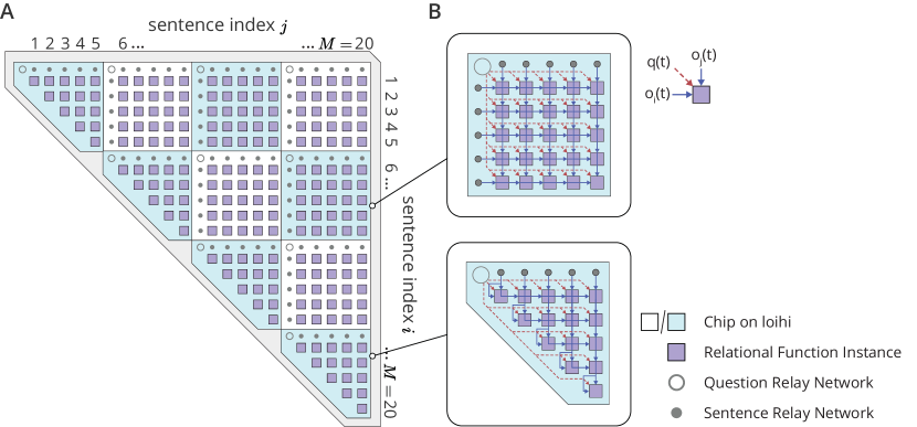
Figure S2: Placement of relay networks and the initial layer of $g_{\theta}$ instances that minimizes spike congestion:   A) Here we show how the first layer of the several instances of the relational function $g_{\theta}$ are placed across the several chips. The instances of $g_{\theta}$ are arranged according to the indices of the input sentences $o_{i}(t),o_{j}(t):i\leq j$. Each blue/cyan block corresponds to a single Loihi chip, within which we show the $g_{\theta}$ instances whose first layer is placed on that chip, along with the relay layers that give them the input. Each cell also has a relay layers for the question embedding $q(t)$. The instances are grouped into squares because this minimizes the number of distinct inputs (i.e. relay layers) needed. B) A blowup of a chip showing the connections between the relay layers and the contained instances of $g_{\theta}$.

References

- [Davies et al., 2018] Davies, M., Srinivasa, N., Lin, T., Chinya, G., Cao, Y., Choday, S. H., Dimou, G., Joshi, P., Imam, N., Jain, S., Liao, Y., Lin, C., Lines, A., Liu, R., Mathaikutty, D., McCoy, S., Paul, A., Tse, J., Venkataramanan, G., Weng, Y., Wild, A., Yang, Y., and Wang, H. (2018). Loihi: A neuromorphic manycore processor with on-chip learning. micro, 38(1):82–99.
- [Santoro et al., 2017] Santoro, A., Raposo, D., Barrett, D. G., Malinowski, M., Pascanu, R., Battaglia, P., and Lillicrap, T. (2017). A simple neural network module for relational reasoning. In Advances in neural information processing systems, pages 4967–4976.
- [Weston et al., 2015] Weston, J., Bordes, A., Chopra, S., Rush, A. M., van Merriënboer, B., Joulin, A., and Mikolov, T. (2015). Towards ai-complete question answering: A set of prerequisite toy tasks. arXiv preprint arXiv:1502.05698.