Longitudinal Study of an IP Geolocation Database

Abstract.

IP geolocation – the process of mapping network identifiers to physical locations – has myriad applications. We examine a large collection of snapshots from a popular geolocation database and take a first look at its longitudinal properties. We define metrics of IP geo-persistence, prevalence, coverage, and movement, and analyze 10 years of geolocation data at different location granularities. Across different classes of IP addresses, we find that significant location differences can exist even between successive instances of the database – a previously underappreciated source of potential error when using geolocation data: 47% of end users IP addresses move by more than 40 km in 2019. To assess the sensitivity of research results to the instance of the geo database, we reproduce prior research that depended on geolocation lookups. In this case study, which analyzes geolocation database performance on routers, we demonstrate impact of these temporal effects: median distance from ground truth shifted from 167 km to 40 km when using a two months apart snapshot. Based on our findings, we make recommendations for best practices when using geolocation databases in order to best encourage reproducibility and sound measurement.

1. Introduction

Determining the physical location of Internet hosts is important for a range of applications including, but not limited to, advertising, content and language customization, security and forensics, and policy enforcement (Katz-Bassett et al., 2006; Huffaker et al., 2011; Wang et al., 2011). However, the Internet architecture includes no explicit notion of physical location and hosts may be unable or unwilling to share their location. As a result, the process of third-party IP geolocation – mapping an IP address to a physical location – emerged as a research topic (Padmanabhan and Subramanian, 2001) more than two decades ago and has since matured into commercial service offerings, e.g.,  (Akamai, 2020; max, 2020; Hexasoft, 2020).

IP addresses represent network attachment points, thus IP geolocation is often inferential. Commercial geolocation providers compete, so the methodologies for creating their databases are proprietary. State-of-the-art techniques include combining latency constraints (Gueye et al., 2006), topology (Katz-Bassett et al., 2006), registries (Padmanabhan and Subramanian, 2001), public data (Eriksson et al., 2010), and privileged feeds (Kline et al., 2020).

This work takes a fresh look at IP geolocation data from a temporal perspective. Specifically, we examine the longitudinal stability of locations in an IP geolocation database, the characteristics of location changes when they do occur, and the extent to which a particular instance of a geolocation database impacts conclusions that depend on locations. To wit, network and systems researchers frequently utilize available IP geolocation database snapshots. However, the date of the snapshot may only loosely align with the time of the lookup operation, or the lookups may span multiple snapshots, e.g., a long-running measurement campaign. We show that snapshots of the same geolocation database separated even closely in time can have a non-trivial effect on research results and findings.

For example, across database snapshots in three month window, we find up to 22% of IP addresses move more than 40km, while coverage (the simple presence or absence of an address in the database) varies by as much as 18%. Despite this temporal sensitivity, the date of the geolocation database snapshot is rarely reported in the academic literature – an omission that we show confounds scientific reproducibility.

As a first step to understanding the temporal characteristics of IP geolocation databases, we define metrics of persistence, prevalence, coverage, and distance. We then analyze 10 years of data from the most popular, publicly available, and frequently used database: MaxMind (max, 2020). Our contributions include:

• A survey of how recent systems and networking literature utilizes and depends on IP geolocation data.

• Defining metrics to understand the Internet-wide stability and behavior of IP geolocation databases.

• The first longitudinal study of a widely used IP geolocation database where we find significant short-term dynamics.

• A case study of prior research that depended on geolocation, showing that the results fundamentally differ based on the instance of the geolocation database used.

• Recommendations for the sound use of IP geolocation data in research.

2. Motivation

To better understand IP geolocation as used in the network and systems research community, we surveyed the academic literature. We performed full-text queries, over all time, on four popular digital libraries for three common geolocation databases, MaxMind (max, 2020), NetAcuity (net, 2020), and IP2Loc (ip2, 2020). Table 1 shows the number of papers in each library. MaxMind is clearly the most popular by an order of magnitude. Therefore the analysis in the reminder of this work focuses on MaxMind.

2.1. MaxMind

Founded in 2002, MaxMind is a commercial entity specializing in IP geolocation and related services. MaxMind offers two IP geolocation databases, one that is free (GeoLite) and one that requires a license (GeoIP). The academic literature predominantly uses the free database, GeoLite.

GeoLite is available as a complete database “snapshot.” Snapshots are currently updated weekly and available for public download. GeoLite snapshots contain variable length IP prefixes, each with an associated geolocation. The geolocation may include country, city, latitude/longitude, and accuracy (in km); however many prefixes only provide a geolocation at the country granularity. This work studies the IPv4 GeoLite databases. Henceforth, we refer to GeoLite (and its successor, GeoLite2) informally as “MaxMind” for simplicity.

2.2. Survey Methodology

We characterized the use of MaxMind across nine systems, security and networking conferences during the five year period from 2016-2020. To find papers in the literature using MaxMind, as well understand how it is used, we adopt a semi-automatic method: first, for a given conference venue, we obtain the complete proceedings and perform a case-insensitive search for the string “maxmind.” We manually inspect each paper found to contain “maxmind” to determine whether the work utilizes the database or is simply referencing MaxMind. For example, in (Kotronis et al., 2017), “maxmind” appears only as a citation to the sentence “Current IP-based geolocation services do not provide city-level accuracy$\ldots$” Only those papers that used MaxMind’s database for their research are included in our survey.

Keeping in mind the variety of research questions and geolocation requirements inherent in the various papers, we sought to distinguish what was being geolocated and at what granularity. We manually extract from each paper the granularity required (country, city, or AS) and the type of IP addresses geolocated (all, end users, end host infrastructure, and router). The “end user” category contains IP addresses belonging to residential users (e.g., (Padmanabhan et al., 2019)), or, more broadly, end users issuing web traffic (e.g., (Papadopoulos et al., 2017)). The “end host infrastructure” category includes addresses belonging to Internet infrastructure, typically web (Deng et al., 2017), proxies (Weinberg et al., 2018), or DNS (Pearce et al., 2017) servers. “Routers” include the IP addresses of network router interfaces. Finally, the “all” category contains papers that geolocate all types of addresses such as (Lee and Spring, 2016; Winter et al., 2019). Note that these sets are mutually exclusive, but a paper can use MaxMind on several types of IP addresses. For instance, (Antonakakis et al., 2017) studies the Mirai botnet where the infected IP addresses can belong to both end users and end host infrastructure.

Table 1. Count of papers referencing geolocation databases in four digital libraries.

	ACM	IEEE	arXiv.org	Springer
MaxMind	171	373	96	162
NetAcuity	10	10	8	7
IP2Loc	3	3	0	0

Table 2. Literature survey of MaxMind use in academic venues (2016-2020). “Affected” column specifies if MaxMind was used in methodology (Y) or for validation (V).

			MaxMind							Affected		Snapshot date specified		Free (F) Paid(P) (N/A))
			Granularity			IP type				Y	V	Y	N	F	P	N/A
Conference	Area	Papers	AS	Country	City	All	End user	End host infrastructure	Router
IMC	Meas.	16	1	13	3	2	5	8	1	12	4	1	15	8	3	6
PAM	Meas.	6	0	2	4	1	1	2	0	5	1	0	6	3	1	2
TMA	Meas.	4	1	0	3	3	0	1	0	3	1	2	2	1	2	1
USENIX Sec	Security	10	0	7	3	0	4	7	0	10	0	2	8	1	4	5
CCS	Security	6	2	1	3	0	1	2	3	6	0	0	6	2	1	1
SIGCOMM	Systems	3	0	1	2	0	3	1	0	2	1	0	3	0	3	0
NSDI	Systems	1	0	0	1	0	0	0	1	1	0	0	1	0	0	1
CoNEXT	Systems	2	1	1	0	1	0	1	0	2	0	0	2	1	0	1
WWW	Web	10	0	7	3	0	4	7	0	10	0	2	8	2	2	6
Total	All	58	7	30	22	8	20	28	6	51	7	6	52	18	18	23

2.3. MaxMind in the literature

Table 2 summarizes our findings. We follow the rhetorical structure of Scheitle et al.  (Scheitle et al., 2018) to classify the impact of MaxMind on the paper’s results.

• Affected “Y” are papers that use MaxMind in their methodology to obtain a result. For example, Papadopoulos et al.  (Papadopoulos et al., 2017) use MaxMind to build a classifier to infer how much advertisers pay to reach users.

• Affected “V” are papers that do not use MaxMind to obtain results, but rather to compare their results. For example, Weinberg et al.  (Weinberg et al., 2018) compare their inferred proxy locations to MaxMind’s locations.

The “Date” column indicates whether or not the paper explicitly provides the MaxMind snapshot date. The last column indicates which MaxMind version is used, either free, paid or if the info was not available.

From a macro perspective, MaxMind is both used at country (53%) and city (37%) granularity. Second, it is mostly used to geolocate end users (35%) and end host infrastructure (49%) rather than routers (9%). Then, the majority of papers (86%) use MaxMind to obtain results, and few (11%) provide the snapshot date. Finally, we see that free and paid version of MaxMind are equally used by the community. Note that the totals do not sum to the number of papers as, e.g., a paper may use MaxMind for both AS and country information (Lee and Spring, 2016), or use both the free and paid version (Gharaibeh et al., 2017).

Lesson

MaxMind is the most popular geolocation database to support other research. Further, the results of many papers may be sensitive to geolocation variation, especially given the lack of snapshot dates, large windows of measurement or data, and no explicit alignment between data collected and the geolocation snapshot.

3. Metrics

In this report, we will: (1) characterize the impact of selecting one geolocation database snapshot rather than a different snapshot in time; and (2) survey the dynamics of snapshots, to gain a deeper understanding of how they change. This section defines the metrics used for these purposes: impact in §3.1 and dynamics in §3.2. We assume that snapshots contain IP prefixes and their associated locations; where necessary we trivially assume the expansion of prefixes to the set of individual addresses within those prefixes. We further make the simplifying assumption the snapshots are uniformly distributed over time with an arbitrary inter-snapshot interval (we achieve this in practice via sampling in §4.1.1).

3.1. Impact: Comparing Two Snapshots

This section provides metrics to answer the practical question: what is the impact of choosing one snapshot rather than another from the same time interval? We define metrics on the basis of two concepts for comparing two geodatabase snapshots: coverage difference and distance distribution. For these definitions:

• Let $A$ be a set of IPv4 addresses.

• Let $L$ be the set of all possible locations present in a geodatabase (either latitude-longitude pairs, cities, or countries).

• Let $M$ be a snapshot of this database, defined as a set of pairs $(x,l)$ that map addresses to locations.

• Let $A_{M}\subset A$ be the set of addresses that appear in snapshot $M$. Each address $x\in A_{M}$ appears in only one pair in $M$.

3.1.1. Coverage difference

Intuitively, coverage difference means the portion of IP addresses that appear in one snapshot or another, but not both. Two identical snapshots have a coverage difference of zero and for snapshots that have no IP address in common, the value is one.

Formally, coverage difference is an extension of the concept of ‘coverage’, which for snapshot $M$ with respect to the set of IPv4 addresses $A$ is:

(1) $$\mathrm{coverage}(M)=\frac{|A_{M}|}{|A|}$$

The coverage difference between two snapshots $M_{i}$ and $M_{j}$ on $A$ is the Jaccard distance between $A_{M_{i}}$ and $A_{M_{j}}$:

(2) $$\mathrm{covdiff}(M_{i},M_{j})=\frac{|(A_{M_{i}}\bigcup A_{M_{j}})-(A_{M_{i}}\bigcap A_{M_{j}})|}{|A_{M_{i}}\bigcup A_{M_{j}}|}$$

3.1.2. Distance distribution

As an address $x$ can appear in one location in one geodatabase snapshot and another location in a second snapshot, we let $\mathrm{dist}(x,M_{i},M_{j})$ be the Haversine distance (Cajori, 1993) between the locations of $x$ in $M_{i}$ and $M_{j}$, using latitude-longitude values for each location. The distance distribution between the two snapshots is the set of distances, one for each address that appears in both snapshots:

(3) $$\mathrm{D}_{\mathrm{dist}}(a,M_{i},M_{j})=\{\mathrm{dist}(a,M_{i},M_{j})\mid x\in A_{M_{i}}\bigcap A_{M_{j}}\}$$

To compare two distance distributions, we define the following metric:

(4) $$\mathrm{distdiff(M_{i},M_{j})=(mean}(\{\mathrm{log_{10}(dist}(a,M_{i},M_{j}))\mid x\in A_{M_{i}}\bigcap A_{M_{j}}\})$$

By taking the mean of the log of the distances, we diminish the possibility for outliers (e.g., distances potentially up to 20,000 km) to disproportionately outweigh lower but nonetheless meaningful distances, e.g., on the order of 100 km. Note that while the median is a more robust statistic, typically more than 50% of the address have zero distance, i.e., did not move between snapshots (§ 5.4). Thus, the mean provides a meaningful non-zero measure. Other metrics that we define on the distance distributions are the quantiles of a distribution, along with the maximum value.

3.2. Dynamics: How do Snapshots Evolve

As will be shown in Sec. 5.4, the choice of one snapshot rather than another can have a large impact, even within a short time interval. We want to gain a deeper understanding of the underlying dynamics of a geolocation system and therefore define the following concepts: the coverage difference between snapshots, the prevalence and persistence of locations, and the distance distribution between snapshots. Whereas the concepts in the previous section concerned pairs of snapshots, in this section we consider sequences of many snapshots generated over time.

3.2.1. Coverage difference

The coverage difference for a set of $n$ geodatabase snapshots $M_{1},...,M_{n}$ is defined to be a value between zero and one as determined by the generalized Jaccard distance:

(5) $$\mathrm{covdif}(M_{1},...,M_{n})=\frac{|\bigcup M_{i}-\bigcap M_{i}|}{|\bigcup M_{i}|}$$

If, for example, the coverage difference is 0.30 over the course of a year, this means that for 30% of the IP addresses, each of those addresses does not appear in at least one snapshot for that year. The lower the coverage difference, informally, the more ‘stable’ we might consider the set of IP addresses as viewed by the geolocation system.

3.2.2. Prevalence and persistence

For location dynamics, we adopt prevalence and persistence metrics that are similar to those originally proposed by Paxson (Paxson, 1997) to capture notions of the ‘dominance’ and ‘persistence’ of a route in the Internet.

Table 3 serves as a basis for illustrating how we have applied these notions. It shows eight time periods and the corresponding locations of two IP addresses, $x$ and $y$. There are three possible locations: $\alpha$, $\beta$, $\gamma$ (which might be city, country, or latitude-longitude pair).

Table 3. Example for prevalence and persistence

Time period	0	1	2	3	4	5	6	7
Location of $x$	$\alpha$	$\alpha$	$\alpha$	$\gamma$	$\beta$	$\beta$	$\beta$	$\beta$
Location of $y$	$\alpha$	$\alpha$	$\beta$	$\beta$	$\gamma$	$\beta$	$\alpha$	$\alpha$

Prevalence

The prevalence of an address $a$ for a location $l$, $\mathrm{prev}(a,l)$ is the portion of time periods at which $a$ is mapped to $l$. Our survey looks at the distribution of prevalence values per address, as illustrated in Table 0(a). These values are frequencies that add up to 1 for each address. For example, address $x$ is mapped to location $\beta$ for 4 out of the 8 time periods, so $\mathrm{prev}(x,\beta)=4/8$.

Our survey also looks at the distribution of prevalence values per location. The same values are simply transposed, as shown in Table 0(b), which is a transposition of Table 0(a). Distributed in this way, the values do not necessarily add up to 1.

Seen in this way, the values give some insight into the likelihood that a mapping to a given location will remain in that location across time periods. A mapping to location $\gamma$ is a rare event, for instance, as reflected in prevalence values of $1/8$ and $1/8$ that are low on average. A mapping to location $\alpha$ can be said to be more likely to be consistent across snapshots, with its prevalence values of $3/8$ and $4/8$ that are higher on average.

Table 4. Prevalence values

$l$	$\alpha$	$\beta$	$\gamma$
$\mathrm{prev}(x,l)$	3/8	4/8	1/8
$\mathrm{prev}(y,l)$	4/8	3/8	1/8

(a)

$a$	$x$	$y$
$\mathrm{prev}(a,\alpha)$	3/8	4/8
$\mathrm{prev}(a,\beta)$	4/8	3/8
$\mathrm{prev}(a,\gamma)$	1/8	1/8

(b)

Formally,

• Let $T$ be the set of time periods.

• Let $\mathcal{L}_{x}$ be the set of pairs $(t,l)$, one for each time period $t\in T$, where the snapshot for $t$ designates $x\in A$ as being at location $l\in L$.

where $A$ and $L$ have the same definition as in Section 3.1. Then the prevalence of an address $x$ at a given location $\alpha$ is:

$$\mathrm{prev}(x,\alpha)=\frac{|\{(t,l)\in\mathcal{L}_{x}:l=\alpha\}|}{|\mathcal{L}_{x}|}$$

and the maximum prevalence of an address $x$ is:

(6) $$max(\{\mathrm{prev}(x,l):l\in L\})$$

To define the distribution of prevalence values for a $l\in L$, we need to define $A_{l}$, the subset of IP addresses with at least one location equal to $l$:

$$A_{l}=\{x\in A:(\exists\ (t,l_{t})\in\mathcal{L}_{x}:l_{t}=l)\}$$

and the distribution of prevalence values is then:

(7) $$D_{\mathrm{prev}}(l)=\{\mathrm{prev}(x,l):x\in A_{l}\}$$

and the mean value of this distribution is then:

(8) $$\mathrm{mean}(D_{\mathrm{prev}}(l))$$

This last metric permits sorting locations by their prevalence.

Persistence

The persistence of an address $a$ for a location $l$, $\mathrm{pers}(a,l)$ is the probability for $a$, to stay in $l$ between two consecutive time periods. Our survey looks at the distribution of persistence values per address, as illustrated in Table 0(c). These values go from 0 to 1, but do not necessarily add up to 1 for each address. For example, when address $x$ is located in $\beta$, it always stays in $\beta$ in the subsequent time period, so $\mathrm{pers}(x,\beta)=1$.

The mean persistence for an address $a$, $\mathrm{mean}(\mathrm{pers}(a))$, is the generalization of $\mathrm{pers}(a,l)$, but for any location $l$. In our example, $\mathrm{mean}(\mathrm{pers}(x))=5/7$ and $\mathrm{mean}(\mathrm{pers}(y))=3/7$.

Like for prevalence, our survey also looks at persistence values per location, as shown in Table 0(d). Seen in this way, it gives some insight into the likelihood that a mapping to a given location will remain in that location in the subsequent time period. For instance, it is very unlikely that a mapping to $\gamma$ will stay in $\gamma$ in the subsequent time period, as the persistence values are 0.

Table 5. Persistence values

$l$	$\alpha$	$\beta$	$\gamma$
$\mathrm{pers}(x,l)$	2/3	1	0
$\mathrm{pers}(y,l)$	1/2	1/3	0

(c)

$a$	$x$	$y$
$\mathrm{prev}(a,\alpha)$	2/3	1/2
$\mathrm{prev}(a,\beta)$	1	1/3
$\mathrm{prev}(a,\gamma)$	0	0

(d)

Formally, by keeping the same notations for $\mathcal{L}_{x}$ and $A_{l}$ defined in the prevalence paragraph, the persistence of an address $x$ at a given location $\alpha$ is:

(9) $$\mathrm{pers}(x,\alpha)=\frac{|\{\{(t,l_{t}),(t+1,l_{t+1})\}\in\mathcal{L}_{x}:l_{t}=l_{t+1}=\alpha\}|}{|\{\{(t,l_{t}),(t+1,l_{t+1})\}\in\mathcal{L}_{x}:l_{t}=\alpha\}|}$$

The mean persistence of an address $x$ is:

(10) $$\mathrm{mean(}\mathrm{pers}(x))=\frac{|\{\{(t,l_{t}),(t+1,l_{t+1})\}\in\mathcal{L}_{x}:l_{t}=l_{t+1}\}|}{|\{\{(t,l_{t}),(t+1,l_{t+1})\}\in\mathcal{L}_{x}\}|}$$

The distribution of persistence values for a location $l\in L$ is:

(11) $$D_{\mathrm{pers}}(l)=\{\mathrm{pers}(x,l):x\in A_{l}\}$$

and the mean value of this distribution is:

(12) $$\mathrm{mean}(D_{\mathrm{pers}}(l))$$

which permits sorting locations by their persistence.

3.2.3. Distance

Prevalence and persistence characterize the dynamics from a discrete point of view; in Table 3, $x$ would have the same values of maximum prevalence and mean persistence whatever the values of $(\alpha,\beta,\gamma)$. We are now interested in studying the distances between these locations.

Our survey looks at the distribution of distance values per address. We define the maximum distance of an address $x$ as being the maximum distance between two of its locations. Formally, the distribution of distances of $x$ is:

$$D(x)=\{\mathrm{dist}(l_{t_{i}},l_{t_{j}}):(t_{i},l_{t_{i}}),(t_{j},l_{t_{j}})\in\mathcal{L}_{x}\}\}$$

and the maximum distance of $x$ is then:

(13) $$\mathrm{max}(D(x))$$

Our survey also looks at the distribution of maximum distance per geographic entity (either a continent, country). For instance, for the addresses that geolocate within a particular country, we wish to understand the maximum distance they move within that country. It allows us to understand if IP addresses tend to have a higher/lower maximum distance depending on which countries they belong. Notice the distinction here between the terms location and geographic entity, as the locations refer to latitude/longitude pairs in this paragraph.

To define the distribution of maximum distance for a geographic entity $c$, we first define the set of latitude/longitude coordinates $L_{c}\subset L$ :

$$L_{c}=\{l\in L:l\ \mathrm{belongs\ to\ }c\}$$

We define the subset of distances $D_{c}(x)\subset D(x)$ as:

(14) $$D_{c}(x)=\{\mathrm{dist}(l_{t_{i}},l_{t_{j}})\in D(x):l_{t_{i}}\in L_{c}\lor l_{t_{j}}\in L_{c}\}$$

The distribution of maximum distance for $c$ is then:

(15) $$D(c)=\{\mathrm{max}(D_{c}(x)):D_{c}(x)\neq\emptyset,x\in A\}\}$$

and the mean of this distribution is:

(16) $$\mathrm{mean}\{\mathrm{log_{10}}(\mathrm{max}(D_{c}(x))):D_{c}(x)\neq\emptyset,x\in A\}\}$$

which permits sorting geographic entities by their maximum distance distribution. Note the presence of $\mathrm{log_{10}}$ for the same reason described in §3.1.2.

Note that from Eq. 15, if an IP address moves from one country to another, we account it for both countries.

4. Data

Before delving into the details of each finding, we present our datasets in Sec. 4.1 and 4.2. Ethical considerations of our work are provided in Appendix A.

4.1. MaxMind snapshots

We collect 214 MaxMind snapshots spanning the ten year period from January 2010 to December 2019. There are two primary challenges in the raw data: (1) the snapshots we obtain are not uniformly distributed in time; and (2) IP addresses appear within prefixes of different networks and lengths over time. To utilize this data within the framework of our methodology and metrics, we pre-processed it.

4.1.1. Sampling the snapshots for time uniformity

Sec. 3 assumes a uniform distribution of snapshots in time. Our evaluation examines a ten year span from 2010-2019. Within this ten year period, we have at least one snapshot per month, but sometimes as many as one snapshot per week. Therefore to ensure uniformity, we simply down-sample so that the ten year period includes one snapshot per month. Our evaluation is conducted on this subset of snapshots such that they are uniformly distributed in time.

4.1.2. Prefixes of different lengths

A MaxMind snapshot contains a mapping of prefixes to geolocation. However, as with prefixes in a routing table, prefixes may split, be aggregated, or even overlap in time. While our analysis is at the per-IP address granularity, rather than prefix, maintaining the geolocation for all IP addresses over time is inefficient. Our first step then is to find a data structure to efficiently store and query the snapshots. Over all prefixes in all snapshots, we construct the set of covering longest length prefixes and construct a Patricia trie (Sklower, 1991). We build one Patricia trie for each geolocation granularity: country, city, and coordinates. The Patricia trie contains, per prefix, all its locations over the period of time.

To handle prefix variation over time, we insert into the Patricia trie the longest prefixes. For example, if for one snapshot, a prefix has a length of 24, and for another snapshot it is split into two prefixes with a length of 25, the two /25 prefixes are placed in the trie and the first snapshot populates both prefixes with the location of the /24.

4.2. Different types of IP addresses

Sec. 2 has shown that researchers use MaxMind to locate three classes of IP addresses: end users, end hosts infrastructure and routers. We therefore collect and label three sets of IP addresses corresponding to these three types.

• End users: M-Lab (mla, 2020) performs and records measurements to end users requesting performance tests (i.e., a “speedtest”). From the M-Lab public datasets we extract targets in the year 2019. We randomly sample these targets to obtain 6.7M IPv4 addresses in approximately 2M unique /24 prefixes.

• End host infrastructure: For end host infrastructure, we extract the daily top list made available by (Scheitle et al., 2018). We perform an intersection of all 2019 lists in order to minimize the number of IP addresses that could be reassigned for other purpose. Because these top lists are volatile, our filtering for high-confidence end host infrastructure addresses produces 26,231 IP addresses in 16,942 /24 prefixes.

• Routers: We leverage both CAIDA ITDK dataset (cai, 2020) and Diamond-Miner (Vermeulen et al., 2020) public Internet topology datasets to collect IP addresses belonging to router interfaces. Both datasets are the result of Internet-wide traceroute style probing. We take the intersection of 2019-01, 2019-04 ITDK and 2019-08 Diamond-Miner datasets and obtain 730k IP addresses in more than 177k different /24 prefixes. By taking the intersection over time, the aim is again to ensure the likelihood that the addresses indeed belong to routers.

5. Evaluation

This section presents an evaluation of ten years of MaxMind data using the metrics defined in the methodology. Our study analyzes if the dynamics depend on three different axes: time, type of IP address and country. Primary results are presented here, while a more exhaustive evaluation along all three of these analysis dimensions, omitted due to space constraints, is available in an accompanying technical report (Anonymous, 2020).

5.1. Prevalence and persistence

As a first step to understanding the MaxMind data, we utilize our primary metrics of prevalence and persistence. Recall that, informally, prevalence is a measure of how frequently an IP address has a given geolocation across snapshots, while persistence is a measure of how long the IP address has a geolocation before it changes. Further recall that for each IP address, the MaxMind data includes a country, city, and latitude/longitude. Thus, these metrics can be computed relative to different location granularities.

(a) By country (Eq. 8)

(b) End users (Eq. 7)

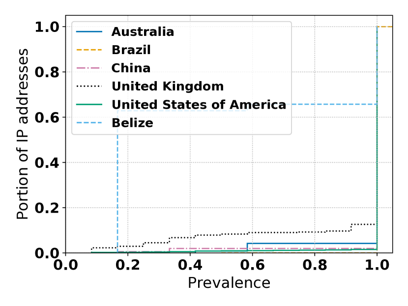
(c) End host infra. (Eq. 7)

Figure 1. Country prevalence measures how frequently an IP address has a given country across snapshots. While prevalence is generally high, it varies significantly for particular subsets of addresses and countries.

5.1.1. Country

We find that for all years, except 2012, more than 98% of the IP addresses have a country-level prevalence of 1, meaning that their country did not change. Note that because the prevalence is very close to 1, the persistence is also close to 1.

However, the prevalence can vary significantly for particular subsets of addresses and countries. Fig. 1(a) shows the cumulative fraction of countries as a function of mean prevalence. Across all classes of IP addresses, most countries have a mean prevalence of more than 0.9, however some in the tail of the distribution have a low mean prevalence, with a minimum of 0.18. Kossovo, on Fig. 1(b) is the country with the lowest prevalence. For end users, countries with low prevalence are mainly found in small Islands. Fig. 1(b) and 1(c) also shows the prevalence distribution for one big country per continent. Note that for end host infrastructure, the prevalence for United Kingdom is lower than for the other big countries: 8% of IP addresses once located in UK had a prevalence for UK of less than 0.6, which is not negligible.

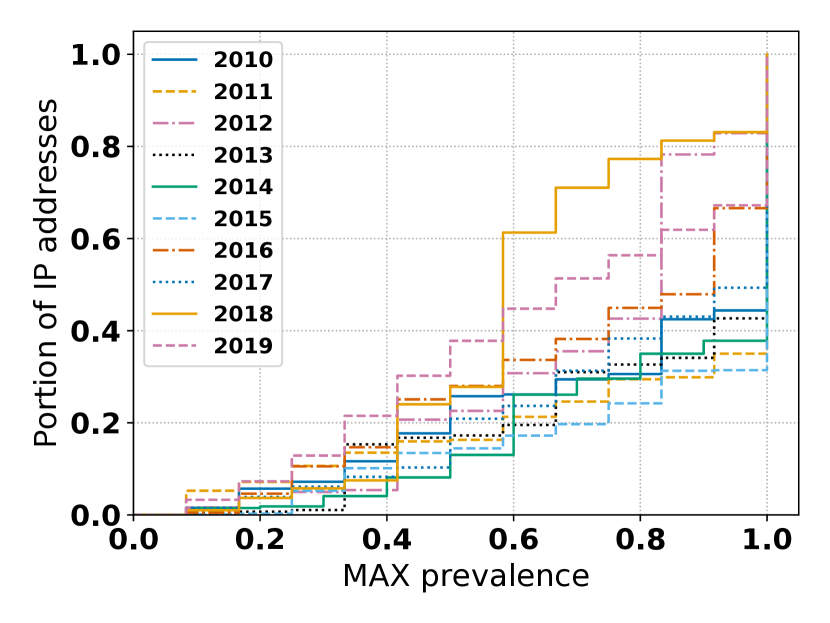
(a) Over time (Eq. 6)

(b) All (Eq. 7)

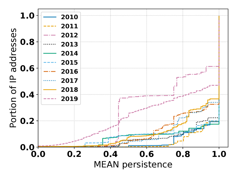
(c) Over time (Eq. 10)

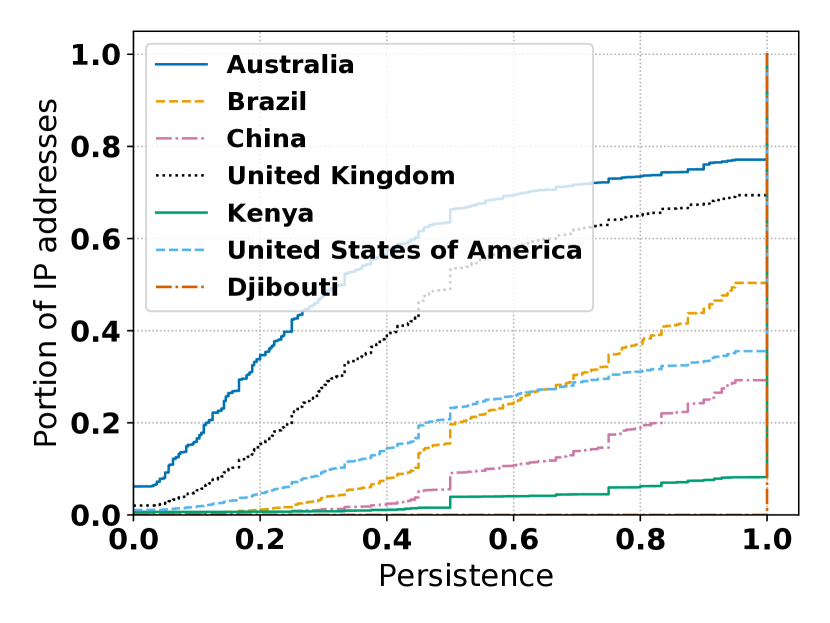
(d) All (Eq. 7)

Figure 2. Decomposing city-level geolocation prevalence and persistence, over time and per country. As compared to country locations, cities exhibit both short and long term dynamics.

Lesson

Statistically, almost all IP addresses have a single country geolocation. However, when restricting by orthogonal axes such as the class of IP address and country, this result is more nuanced. MaxMind locations in such countries should be used with caution. There is a significant chance that the country may change for these IP addresses during the year.

5.1.2. City

Fig. 2(a) shows the CDF of maximum prevalence at the city-granularity from 2010 to 2019 per IP address. In contrast to the country-level, at the city-level granularity, the CDF is not concentrated at a prevalence of 1. In 2019, we observe that 38% of the IP addresses have a maximum prevalence of less than 0.5, meaning that they do not have a dominant city. Note that this result holds for all types of IP addresses.

As we did for prevalence at country level, Fig. 2(b) shows the results for the same five countries, plus the country with, this time, the highest mean prevalence. The prevalence distribution for the five countries is not anymore all concentrated near one, and that at maximum, only 54% of IP addresses have a prevalence of one, corresponding to US. Conversely, notice that for Korea, the prevalence distribution is located near one. We observed that other countries with high city mean prevalence were likely African countries. One hypothesis is that MaxMind have less information for these countries and then IP addresses are less likely to change their location.

Fig. 2(c) shows the CDF of the mean persistence per year from 2010 to 2019. We observe that the curve of 2019 is above all of the others, except 2012, so the mean persistence in 2019 was lower. 30% of the IP addresses have a mean persistence under 0.5, while 50% have a mean persistence of 1. This wide spectrum of mean persistence values show that both short and long term city location changes exist. Note that this result holds for all types of IP addresses, although we noticed that end host infrastructure had a higher persistence in general than the other types of IP addresses.

Again, we dig into the data to study if the city-level persistence depends on the country. Fig. 2(d) shows mean persistence for the five countries, plus the one having the highest mean persistence. Notice the example of Kenya that has a higher mean persistence than the other countries. We observed that again, African countries tend to have a higher mean persistence than countries on other continent.

Lesson

The prevalence results show that the majority of IP addresses covered by MaxMind are not mapped to a single city during the 2019 year. The wide range of values for persistence show that there are both short and long term city changes.

5.2. Distance

(a) Over time (Eq. 13)

(b) By IP class (Eq. 13)

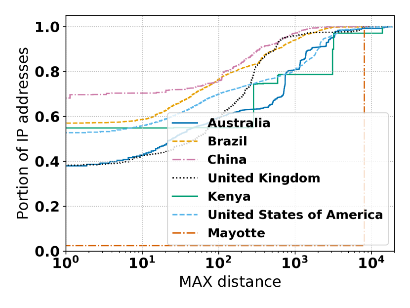
(c) Routers (Eq. 15)

Figure 3. Quantifying distance (km) dynamics over time, IP class, and selected countries. While most distance changes are $\leq$40km, there are classes of addresses and countries with significantly higher movement.

Results of the previous section on prevalence and persistence of the MaxMind city database show that per-IP city geolocations are highly dynamic. In this subsection, we quantify the distance of these changes. In contrast to Section 5.4 that analyzes the distribution of distance differences between two snapshots separated by different hypothetical intervals of time, here we analyze the complete dynamics of the latitude / longitude coordinates over time as present in MaxMind. For instance, whereas the previous analysis considers the distance change over all addresses in the two snapshots, here we consider the maximum distance change for each IP address across all snapshots.

5.2.1. The maximum distance distribution is highly variable between years

Fig. 3(a) shows the distribution of the maximum distance between two locations of an IP address during each year from 2010 to 2019. We do not observe any trend in distance change over time and each year exhibits a different distribution. For instance, in 2018, 42% of the IP addresses had a maximum distance change of more than 40km, whereas only 22% had this much movement in 2019. The year 2012 is an outlier with 40% of the IP addresses having a maximum distance change of more than 1000km.

5.2.2. The maximum distance depends on the type of IP address and the country

Fig. 3(b) shows the maximum distance change distribution in 2019 as a function of IP address class. We observe that the distribution depends on the IP address type for distances under 1000km. End user IP addresses experience the most significant changes; 47% have a maximum distance of more than 40km, as compared to 11% for end host infrastructure and 28% for routers.

We investigate the maximum distance of our five countries. Fig. 3(c) show the distance change distributions for routers. Here again, we observe that the results are largely dependent on the country: 28% of IP addresses in China have a maximum distance of more than 40 km, whereas it is 36% for IP addresses in US, and 50% for the United Kingdom.

Lesson

Distance change results bring additional insights to country and city dynamics. Again, if statistically, a majority of IP addresses have a maximum distance change less than 40km, digging into the data reveals a high disparity between IP address type and country with respect to geolocation change distance.

5.3. Visualizing Internet-wide geo movement

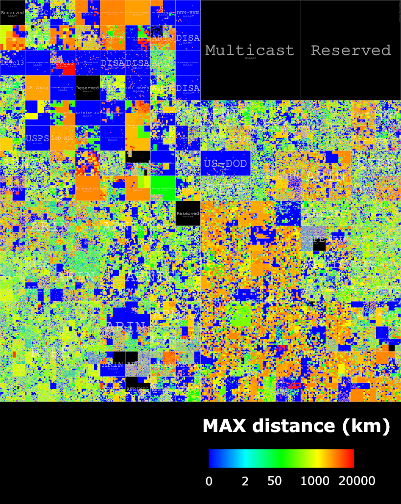
Figure 4. Hilbert heatmap of maximum distance on a logarithmic scale (Eq. 13) in 2018 (left) 2019 (center) and absolute difference (right). There is a high degree of global geolocation dynamics and year-to-year variation.

Fig. 4 shows an exhaustive representation of the maximum distance change for each /24 of the entire IPv4 space for 2018 and 2019, as well as the absolute difference between the two years. Each pixel represents a /24, and the color represents the maximum distance between two locations; black pixels indicate that the IP address is not present in the database. If the /24 contains more specific entries in the MaxMind database, we take the maximum of the maximum distance of the IP addresses within the /24.

We see that the visualization of 2019 differs from 2018: Many of the various registries in the bottom center right and top left part of the plots have a maximum distance of more than 1000km in 2018, whereas they did not move in 2019. There is also a red square in the prefixes belonging to Level3, that had a maximum distance of 20,000km in 2018 but did not move in 2019.

Surprisingly, there are also some IP addresses that were covered in 2018 (i.e., in this case, having lat/long coordinates) which are not covered in 2019. This is the case of some blocks of IP addresses in the bottom center left of the graph belonging to APNIC and AFRINIC.

All these differences between the two years are highlighted by the map on the right: we clearly see the center and the bottom left mainly colored in orange and red as well as some big prefixes on the top right. It reveals a significant dynamic changes not only along the prefixes but also through time.

Overall, by looking at the Hilbert representations of each year over the 10 years dataset, it is difficult to perceive a trend that could lead us to say that prefixes are experiencing bigger or smaller distance change over years.

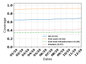
Figure 5. Coverage by address type

Finally, we consider a different notion of coverage – the coverage relative to routed IP address space. To assess routed address space coverage, we utilize the global BGP tables available from Route Views (rou, 2020) coinciding with the date of each MaxMind snapshot. Fig. 5 shows two things: first, the overall coverage is relatively constant over time for all classes of IP addresses. However, the coverage value strongly depends on the type of address. There is about 90% coverage for end users, 37% for end host infrastructure and 41% for routers. The Jaccard distance is interesting: going from 0.16 for end users, to 0.47 for routers. This means that even if the coverage is constant over time, the set of IP addresses covered varies significantly.

Lesson

These visualizations confirm not only the high degree of global geolocation dynamics, but also the presence of year-to-year variation in geolocation movement. An IP address can experience a maximum distance change of 0km in 2018 and more than 1000km in 2019, and vice versa. Also, depending of the address type, the BGP coverage will change significantly.

5.4. Impact

While the preceding analysis demonstrates how our metrics can shed light on the underlying dynamics of a geolocation database, we conclude this section with an analysis of the potential impact of selecting a particular snapshot of MaxMind versus a different snapshot, for instance as a researcher seeking to geolocation a population of IP addresses under study.

To bound our results, we compare pairs of snapshots from 2019 within three time windows: when the snapshots differ by less than 3 months, between 3 to 6 months, and between 6 to 12 months. We evaluate the impact across the four IP classes: all IP addresses (“All”), end users, end host infrastructure, and routers.

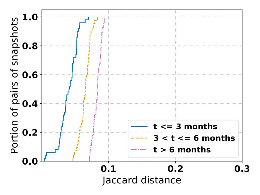
(a) End users

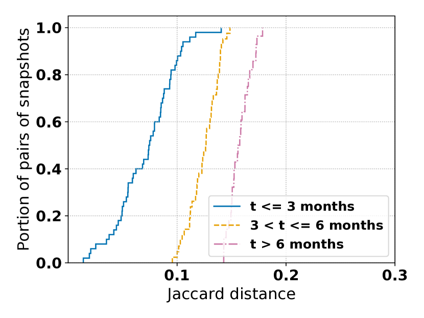
(b) End host infrastructure

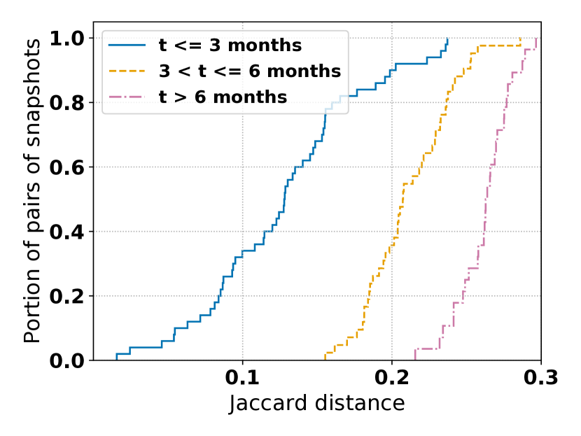
(c) Routers

Figure 6. Comparing pairs of database snapshots by city coverage difference (Eq. 2). Across all classes of IP addresses, there are significant coverage differences, even on among snapshots closely separated in time.

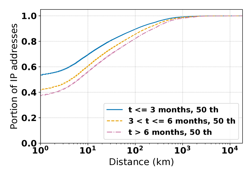
(a) End users

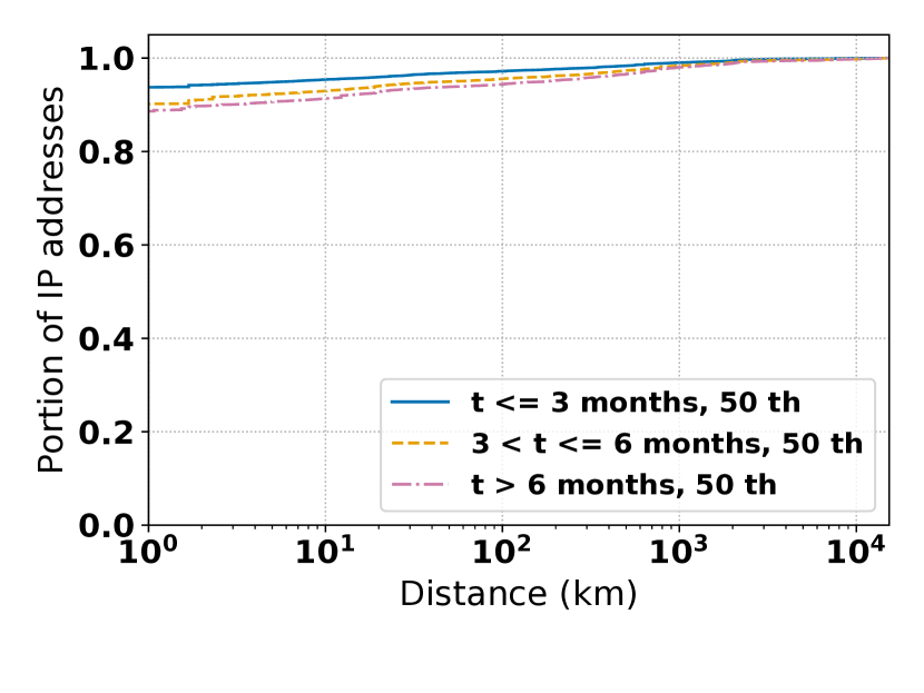
(b) End host infrastructure

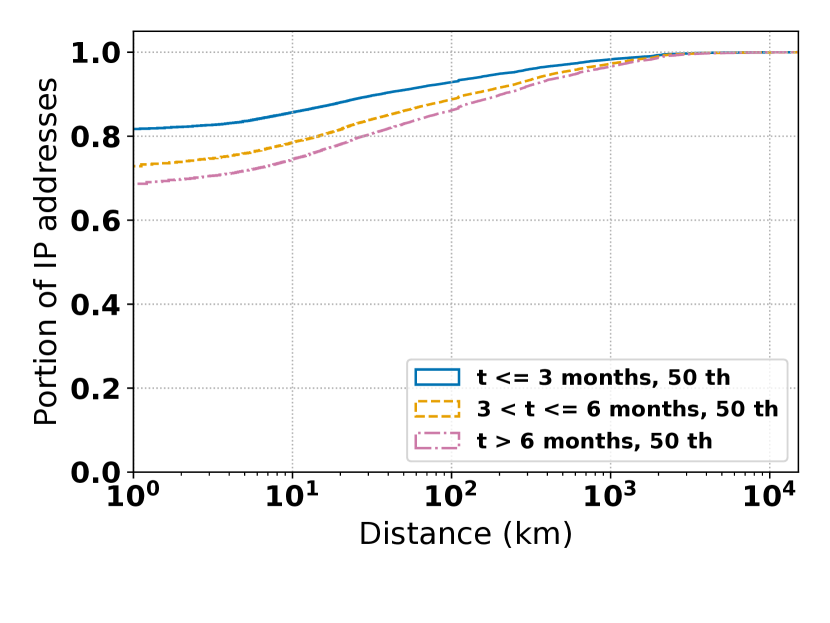
(c) Routers

Figure 7. Comparing pairs of database snapshots by IP address distance difference (Eq. 3). Up to 22% of addresses move more than 40km among snapshots in a three month window.

5.4.1. Coverage (Fig. 6)

For coverage we show results at the city level as we find no country level coverage differences between snapshots; almost all IP addresses, across all classes of addresses, have a country geolocation present in the database.

Not unexpectedly, for all types of IP addresses, we observe that the coverage difference increases with time between the two snapshots. The overall coverage being globally constant (see Fig. 5), this cannot be imputed to an increase of the total coverage.

We see that even for two snapshots created within less than three months of each other, there is a significant coverage difference, up to 6%, 11% and 20% for end users, end host infrastructure and routers respectively. As seen in Fig. 6(c), there is a 50% probability of more than 12% coverage difference between two snapshots created less than three months apart. Between two snapshots of more than six months and less than a year, the difference can be even worse, up to 9%, 17% and 30%.

5.4.2. Distance (Fig. 7)

We first sort the pairs of snapshots by the metric defined in Eq. 4, the mean of the logarithmic distances (MLD). Recall, the higher the MLD, the more the snapshots differ. We compute distance across pairs of snapshots within the same time ranges as for coverage: less than three months, between three and six months, and between six and twelve months. From the MLD distribution, we then show the pair of snapshots corresponding to the median. For example, in Fig. 7(a), one should read: On the end users dataset, 15% of the IP addresses moved by at least 40km. This corresponds to the median result for a pair of snapshots that are less than three months apart.

Fig. 7 shows two trends. First, as one might expect, for all types of IP addresses, the more time between two snapshots, the more IP addresses move. Then, the percentage of IP addresses moving depend on the type of IP addresses. We observe that end users tend to move more than routers and end host infrastructure. In details, for a pair of snapshots that are more than six months apart, we have 28%, 8% and 18% of IP addresses that move more than 40km for respectively end users, end host infrastructure, and routers.

If we consider that 40km corresponds to most metropolitan areas (Gharaibeh et al., 2017), this implies that a non-trivial portion of IP addresses experience a location change out of the metro area – a significant change. However, distances greater than 1000km are rare, accounting for less than 5% of IP addresses across all addresses classes.

Lesson

There are non negligible differences in both coverage and distance of movement even for database snapshots created closely in time (¡ 3 months). Therefore: we recommend, insofar as possible, aligning geolocation database snapshots with the measurements that produced them, for instance by programatically using an API to lookup IP addresses on-demand as they are gathered. Further, one should look at several snapshots closely spaced in time over the measurement period and more deeply investigate IP addresses that experienced significant changes.

6. Use Case

Previous sections have shown two things. MaxMind is a widely used database (Sec. 2), and selecting a particular snapshot in a time period can have a significant impact on the results (Sec. 5). In this section, we concretely demonstrate the potential impact on research that depends on MaxMind by reproducing the results from Gharaibeh et al. ’s IMC 2017 work (Gharaibeh et al., 2017) with different MaxMind snapshots. Gharaibeh et al. study the accuracy of different databases for router geolocation, including MaxMind. Using the author’s publicly available ground truth, we reproduce their accuracy results (see Sec. 5.2, Fig. 2 of (Gharaibeh et al., 2017)).

Surprisingly, the MaxMind snapshot that produces the largest impact on the results was created within only two months of the snapshot used by the authors. This snapshot shifts the median of the distance distribution to ground truth from more than 100 km to 40 km, which is close to the results of the paid version. Given this variability, the claim that the free version of MaxMind is worse than the paid version seems to depend on the specific instance studied.

6.1. Dataset

The Gharaibeh dataset consists of 16,586 router interface IP addresses with corresponding ground truth locations inferred either with RTT-based measurements or DNS-based techniques. The authors do not mention which specific snapshot of MaxMind they used, however: “The databases are accessed again on early July 2016, to geolocate the ground truth.” We inquired with the authors for the exact snapshot date, but unfortunately they could not be more specific. We therefore select the closest snapshot as our reference, from July 8, 2016. Sec. 6.2 confirms that the results of this snapshot are very close to those presented in the original paper.

The measurement period for the ground-truth collection and validation, however, spanned a larger time period. As stated in the paper: “Overall, between May 2016 and September 2017, 8,197 (69.1%) […] have different hostnames, and 6.9% no longer have rDNS records.” We therefore restrict our comparison between snapshots belonging to this period of time, on which the authors consider that the ground truth is valid.

6.2. Results

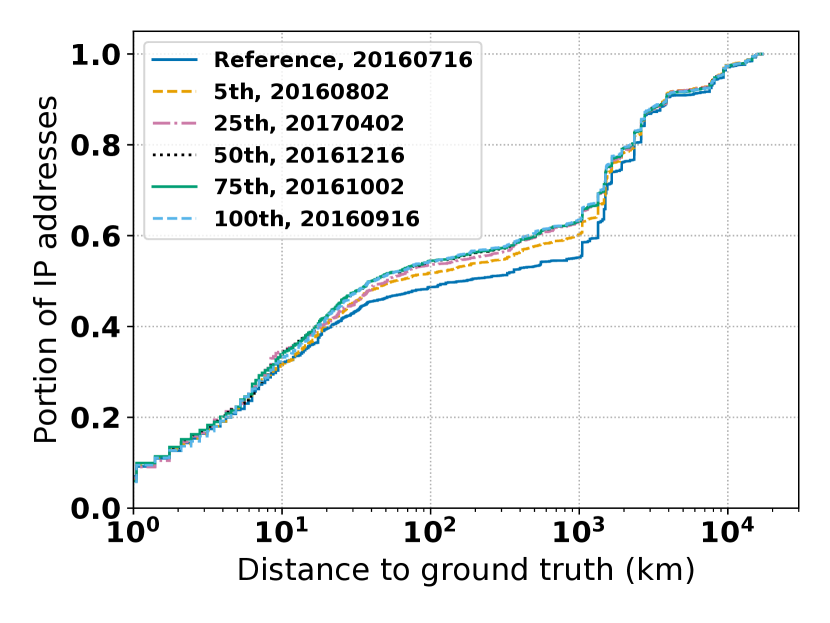
(a) Distance to ground truth CDF on different snapshots

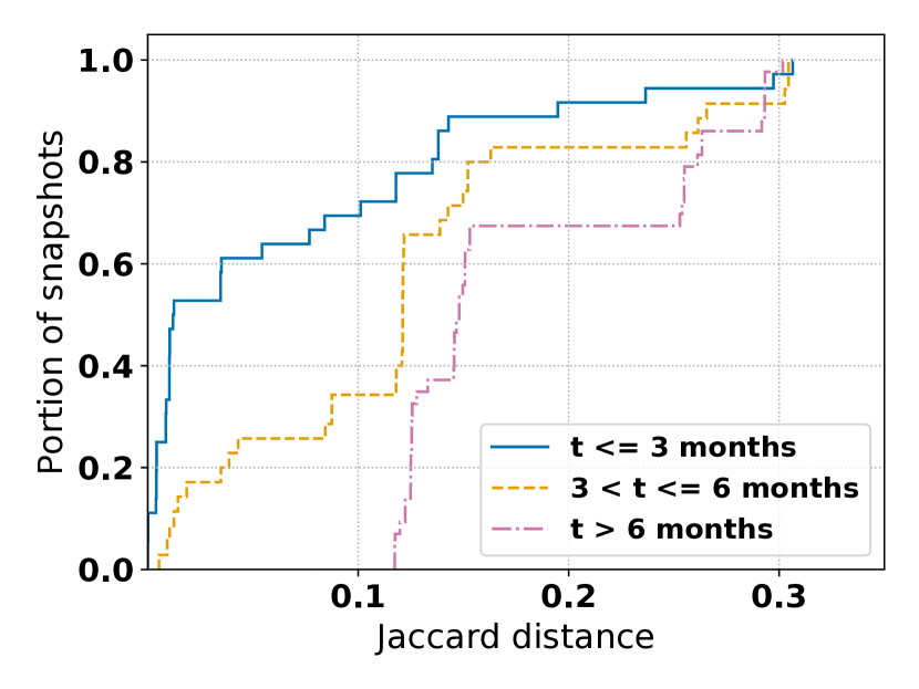
(b) Coverage difference on city with the reference snapshot

Figure 8. Reproducing result of (Gharaibeh et al., 2017) with different snapshots

6.2.1. Distance to ground truth

We compute the distance to ground truth distribution of all the snapshots from May 2016 to September 2017. We then compare each of these distributions to the distribution of the reference snapshot, using the Kolmogorov-Smirnov (KS) test (Lilliefors, 1967). The KS test quantifies how dissimilar are two distributions, with higher values indicating less similarity. Fig. 8(a) shows the distance to ground truth distribution of the snapshots corresponding to the 5th, 25th, 50th, 75th, and 100th percentiles of the KS distribution. We also show the reference snapshot.

First, we compare Fig.2 of Gharaibeh et al. . with our reference snapshot. We infer that on Fig.2 of Gharaibeh et al. ., $\sim$8%, 47%, 50%, 55%, and 96%, are located at less than respectively 1, 40, 100, 1,000, and 10,000km from the ground truth, whereas it is 8%, 46%, 49%, 56% and 97% in our reference snapshot. Overall, the shape of the distribution looks the same, so this give us confidence that our July 8th snapshot is a good reference.

Then, we observe that there are significant differences between the other snapshots and the reference. The median shifts from 167km in the reference snapshot to respectively 57, 51, 41, 40 and 40km for the 5th, 25th, 50th, 75th and 100th percentile.

When we consider the snapshots dates with these percentiles, it is surprising to observe that the 100th percentile was created only two months after the reference snapshot, whereas the 5th percentile is a snapshot taken one month later and the 25th percentile corresponds to a snapshot taken nine months later. This implies that MaxMind did not improve over time for these addresses, but also that there are significant differences in the results within a relatively short time.

Finally, we look at the comparison between the free and paid version of MaxMind. On Fig.2 of Gharaibeh et al. we infer that the paid version has a median between 30 and 40km, so that the difference between this distribution and the different snapshots of Fig. 8(a) is less pronounced than the difference between the free and paid version of their graph. Therefore the conclusion that the paid version performs better than the free one should be taken with caution.

6.2.2. Coverage

Finally, we are interested to compute the variability in coverage as defined in §3.2.1. In Gharaibeh et al. , the authors only compute the distance to ground truth if the IP address is covered by MaxMind at the city level.

Fig. 8(b) shows the distribution of the coverage difference (Eq. 2) as we did in §. 5.4.1, but only comparing snapshots with the reference snapshot. We observe that even with snapshots taken 3 months apart from the reference snapshot, 77% of the snapshots have more than 23% of coverage difference. It is even worse for snapshots between 3 and 6 months and snapshots with more than 6 months of difference, with a coverage difference of about 30%. This means that if the authors had used a different snapshot, the set of IP addresses over which they would have computed their accuracy measures would have significantly changed.

7. Related work

Mapping IP addresses to the physical world is an important topic that has seen two decades of research. Early efforts used landmarks, hosts with known position, to assign locations to unknown targets at coarse granularity (Padmanabhan and Subramanian, 2001). Landmark-based geolocation was subsequently enhanced to use latency constraints (Gueye et al., 2006), network topology (Katz-Bassett et al., 2006), and population densities (Eriksson et al., 2010) to improve accuracy. Because the accuracy of latency-based techniques is often proportional to the distance between the target and its nearest landmark, Wang et al. developed techniques to find and utilize additional landmarks (Wang et al., 2011).

IP geolocation has since matured, with several competing commercial offerings including (Akamai, 2020; max, 2020; Hexasoft, 2020). While the exact methodology of these commercial services is proprietary, they likely use a combination of databases (e.g., whois and DNS), topology, latency, and privileged data feeds from providers (Kline et al., 2020).

Even so, the inference-based nature of IP geolocation imparts errors and inaccuracies even in commercial databases (Huffaker et al., 2011; Shavitt and Zilberman, 2011). demonstrated by several prior analyses. For instance, Poese et al. found 50-90% of ground-truth locations to be geolocated with greater than 50km of error (Poese et al., 2011); most recently Komosnỳ et al. studied eight commercial geolocation databases and found mean errors ranging from 50-657km (Komosnỳ et al., 2017). Geolocation of network infrastructure, including routers, is known to be particularly problematic (Huffaker et al., 2014; Gharaibeh et al., 2017). However, as shown in Sec. 2, MaxMind is still widely used, for the simple reason that there exists no other alternative than geolocation database to get an Internet scale IP geolocation mapping.

Our work looks at IP geolocation through a novel lens by analyzing the longitudinal characteristics of a popular geolocation database. By showing the stability of locations at different granularities and timescales, we offer a first look at the error bounds for particular classes of applications that utilize geolocations, as well as offer practical lessons for consumers of IP geolocation data.

8. Conclusion

Physical mapping of Internet hosts and resources is critical in this day and age. Techniques to perform IP geolocation have matured into commercial offerings. While the accuracy of these geolocation databases has been extensively studied, little attention has been paid to understand the way they have evolved over time. Our work demonstrates that a commonly used geolocation database, MaxMind, exhibits significant changes in coverage, persistence, and prevalence, especially when considering particular subsets of addresses.

These changes can occur even on short timescales, including on the order of a typical measurement study duration. In this way we highlight the importance of geolocation lookups that are contemporaneous with the time an IP address is measured, observed, or gathered. Via a case study, we demonstrate the potential for a large discrepancy in results depending on the particular date of a geolocation snapshot. Similar large variances in auxiliary data sources at short time scales have been demonstrated in the past, e.g., for DNS and Internet top lists (Scheitle et al., 2018). Thus, a take-away of our work is to encourage alignment of geolocation lookups with measurements, publishing the exact date of a geolocation snapshot or lookup methodology, and rigorously investigating addresses that change geolocation significantly over the course of a measurement study. In the spirit of similar measurement best practices (Paxson, 2004), we hope to encourage more sound and reproducible measurement research. Because MaxMind does not provide access to historical data, we provide historical snapshots on demand to the community.

In future work, we plan to more deeply investigate the root causes of the geolocation movement we observe, characterize IPv6 geolocation, and work toward integrating our findings into more robust geolocation services. Finally, we believe the metrics we developed generalize and could be applied to not only other geolocation databases, but also to understand the longitudinal behavior of other dynamic Internet resources such as reverse DNS records. ../code/resources/

Appendix A Ethical Considerations

Our work does not involve human subjects, questionnaires, or personally identifiable information, and, hence, does not meet the standards for IRB review. The MaxMind data we analyze is covered by the Creative Commons Attribution-ShareAlike 4.0 International (CC BY-SA 4.0) license which permits adaption of the database: “remix, transform, and build upon the material for any purpose, even commercially.” Beginning in January 1, 2020, MaxMind adopted a more restrictive policy in order to comply with GDPR requirements (max, 2019); our research does not analyze any data after 2019.

Appendix B Exhaustive Evaluation

In Sec. 5, we only show the primary results that support our main findings. However, we have performed a thorough evaluation of each metric defined in Sec. 3 over three axes: time, type of IP address and location. We put here the whole set of results.

B.0.1. Prevalence on MaxMind country database

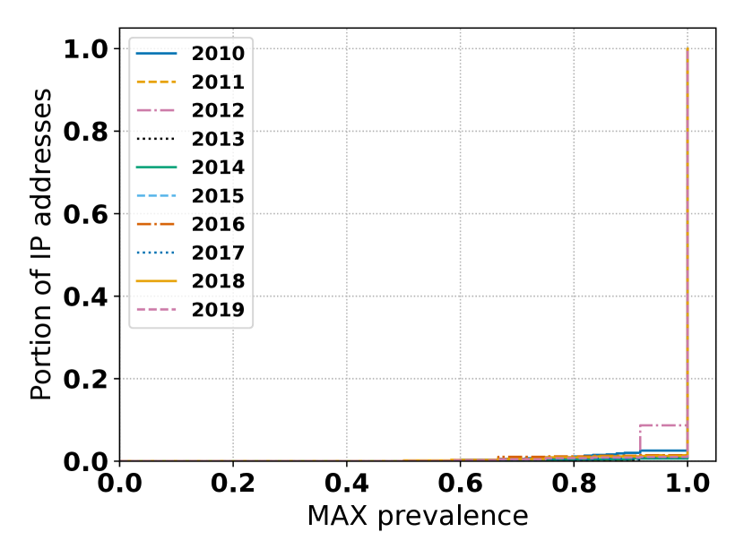
(a) Over time (Eq. 6)

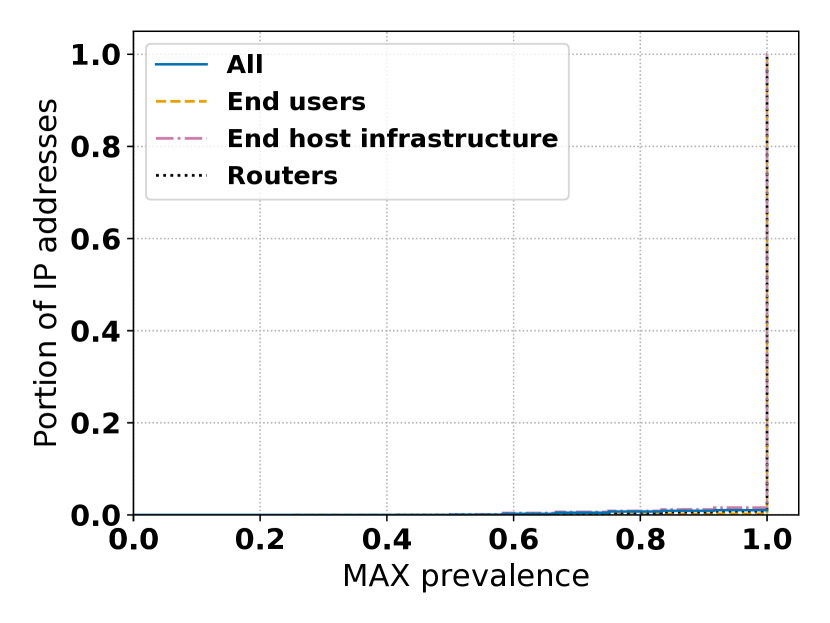
(b) By IP class (Eq. 6)

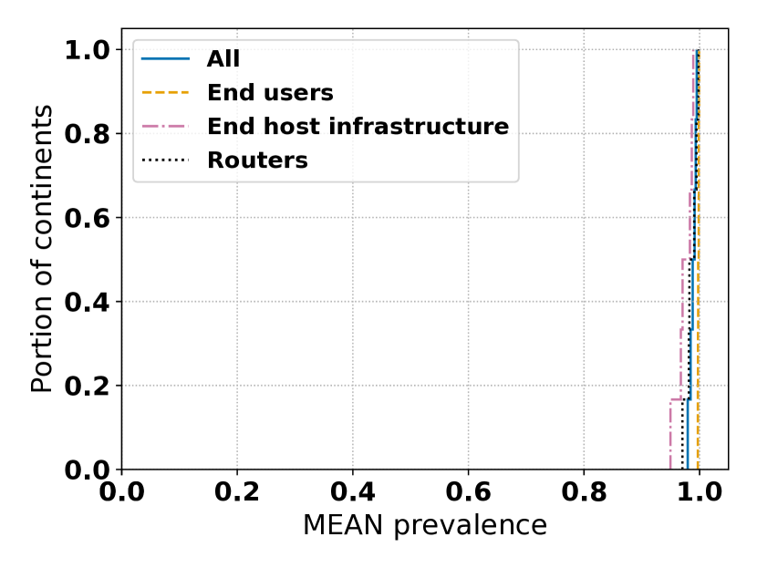
(c) By continent (Eq. 8)

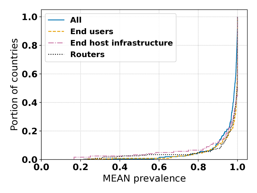
(d) By country (Eq. 8)

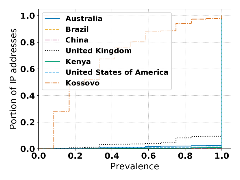
(e) All (Eq. 7)

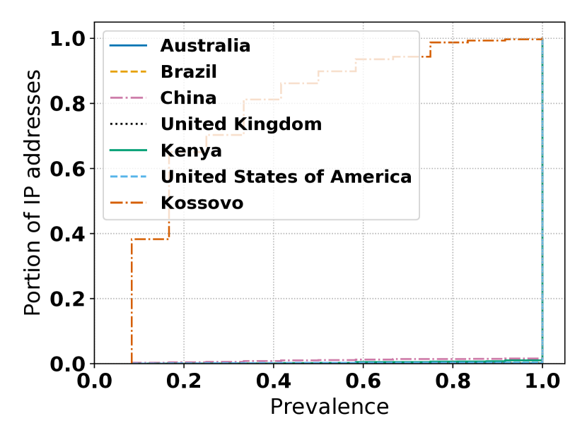
(f) End users (Eq. 7)

(g) End host infra. (Eq. 7)

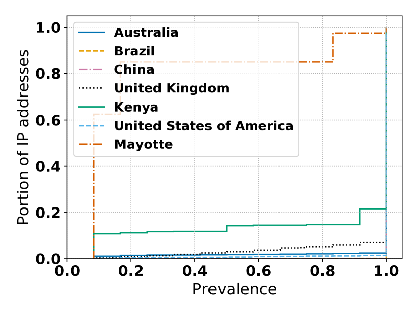
(h) Routers (Eq. 7)

Figure 9. Prevalence results on MaxMind country geolocation

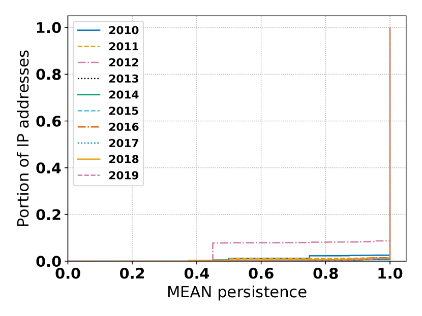
(a) Over time (Eq. 10)

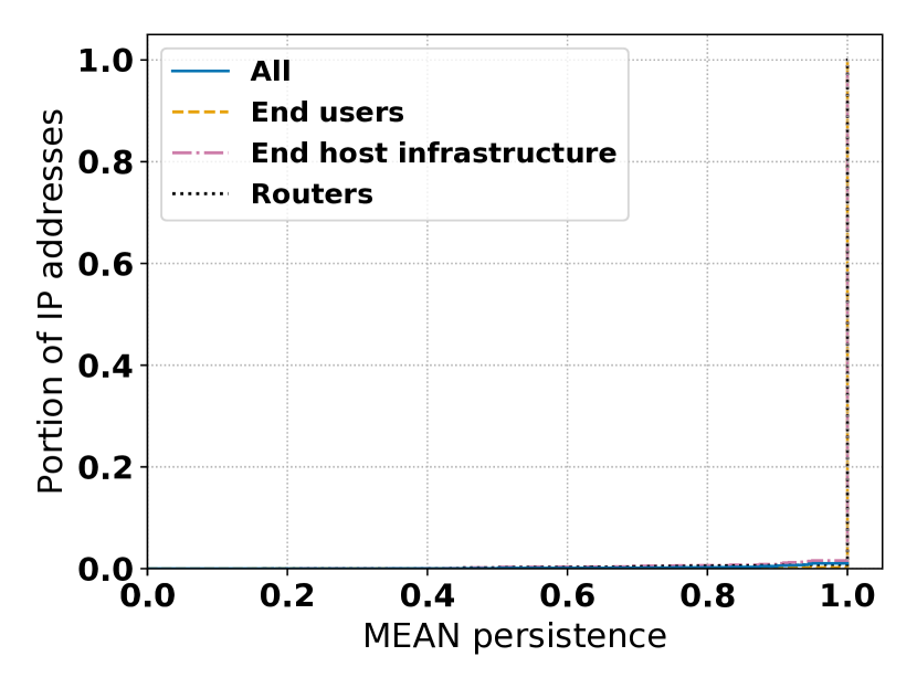
(b) By IP class (Eq. 10)

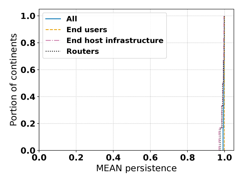
(c) By continent (Eq. 12)

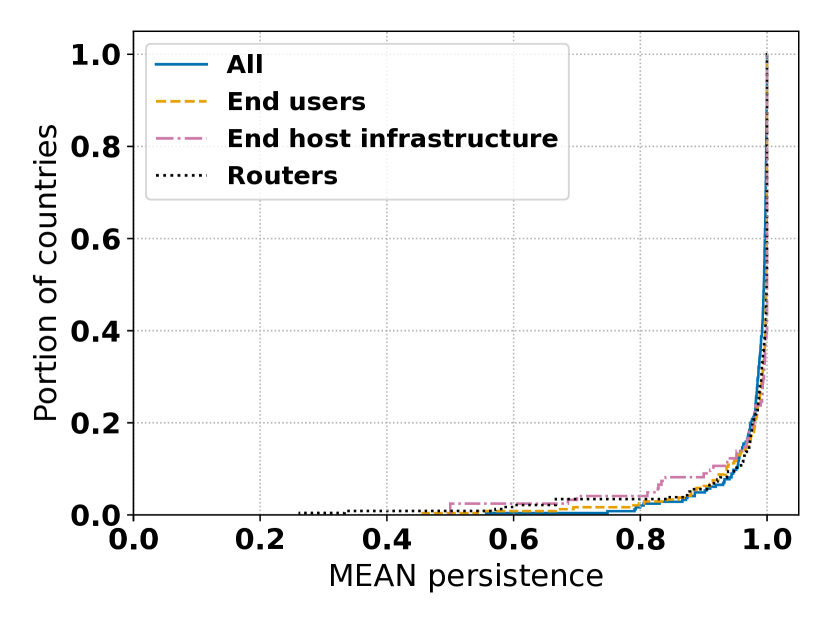
(d) By country (Eq. 12)

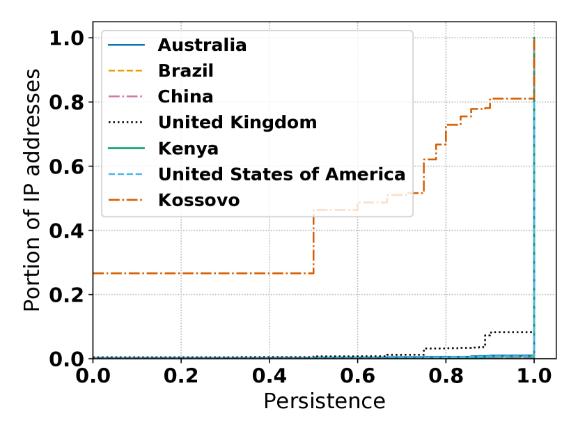
(e) All (Eq. 11)

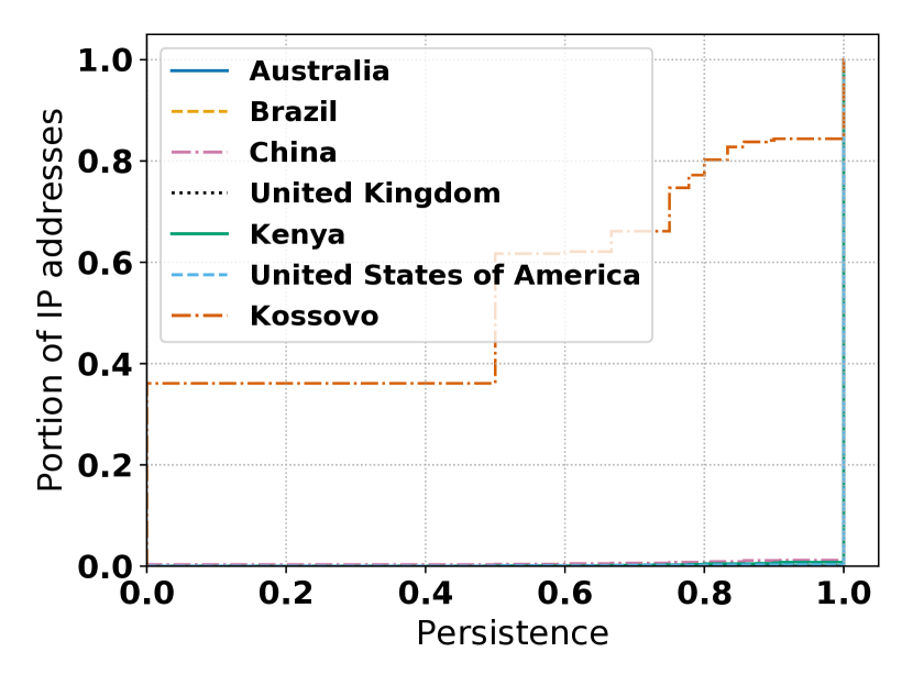
(f) End users (Eq. 11)

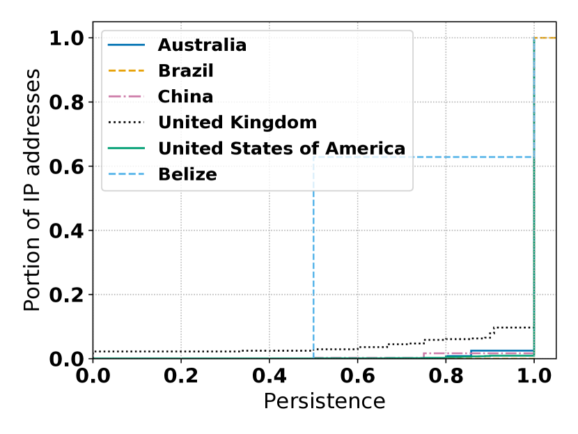
(g) End host infra. (Eq. 11)

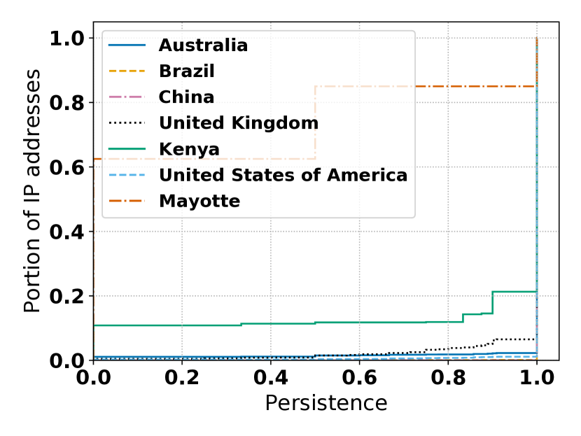
(h) Routers (Eq. 11)

Figure 10. Persistence results on MaxMind country geolocation

Fig. 9 shows our results on the prevalence for the MaxMind country database. As our metrics are built to do so, we vary three orthogonal axis to evaluate the prevalence: the time (2010-2019 and 2019) the prevalence on different types of IP addresses, and the prevalence per geographic location. The two latter focus on the 2019 year.

On each title of each paragraph, we put in parenthesis the corresponding figure and metric defined in Sec. 3.2 that it analyzes.

Evolution of the prevalence (Fig. 9(a), Eq. 6)

We see that for all years, except for 2012, the maximum is concentrated close to 1. This means that IP addresses located by MaxMind have always had a single country.

Per type of IP addresses (Fig. 9(b), Eq. 6)

There is no noticeable difference between all types of IP addresses, the maximum prevalence being close to 1.

Per geographical locations (Fig. 9(c) , 9(d), Eq. 8)

We analyze if the prevalence of country depends on the geographic locations at two levels: the continent and the country.

Fig. 9(c) and 9(d) shows the CDF of the average value of the prevalence for each location for each of our dataset (“All” being the full MaxMind snapshot of the year 2019.). We observe that at continent level, all the continents have a average prevalence close to 1.

At country level, this distribution states that for all 4 types of IP addresses, the tail of the distribution has a low average prevalence, so that there are potentially important differences depending on the country. We deeper investigate these differences in the next paragraphs.

Detailed investigation on continent (Second row of Fig. 9, Eq. 7)

At continent level, interestingly we can see that on the “All” dataset, the distribution for Europe is slightly above the others; 4% of IP addresses in Europe have a prevalence of less than 0.6. This means that 4% of IP located in European countries do not have a single country.

Interestingly, the prevalence per continent also depend on the type of IP addresses: On end users, the prevalence is almost always 1. On end host infrastructure and routers, the curve of Africa is slightly above the other continents; 9% of IP addresses located in Africa do not have a single country.

Detailed investigation on countries (Third row of Fig. 9, Eq. 7)

These graphs show the 10 countries having the lowest average prevalence (Eq. 8).

First, we see that for all of these 10 countries, for each type of IP address, the prevalence is no longer concentrated near 1.

On the “All”, end users, and routers dataset, we can observe that the countries having a low mean of maximum prevalence are rather small, typically islands. Notice however the presence of Netherlands for the routers.

The results on end hosts infrastructure are more surprising. The 10 countries are mainly located in Europe, with Norway, Luxembourg, and United Kingdom for Western Europe and Bulgaria, Lithuania, Moldova, and Czech Republic for Eastern Europe. Notice also the presence of big countries on other continents, such as Argentina.

We evaluate the persistence with the same methodology as for the prevalence, with the three same axes.

The two first rows of graphs of Fig. 10 have nearly the same shape at those on prevalence, meaning that: The average persistence at country level is high. This is mainly due to the high maximum prevalence shown in the previous paragraph; all IP addresses have a single country.

Detailed investigation on countries, third row of Fig. 10, Eq. 11

The third row, focusing on countries having a lower average persistence, reveals the duration of these country changes. First, the countries having the lower average persistence are also the ones that had the least prevalence. Noticeably, we find the same surprising European countries for end host infrastructure, Italy added. Then, we observe that the persistence of these countries depend on the type of IP address. In general we observe that for end users, the curves of the countries are higher than the ones for end host infrastructure and routers, meaning that they have a lower persistence. In details, only Belize for end host infrastructure and Mayotte and Nothern Mariana Islands for routers have more than 20% of IP addresses having a persistence of less than 0.5, whereas there are at least 5 countries for end users.

Our interpretation is that when there is a country change on countries having a low average persistence, the changes are more likely to last for end host infrastructure and routers, whereas they are more likely to be short for end users.

(a) Over time (Eq. 6)

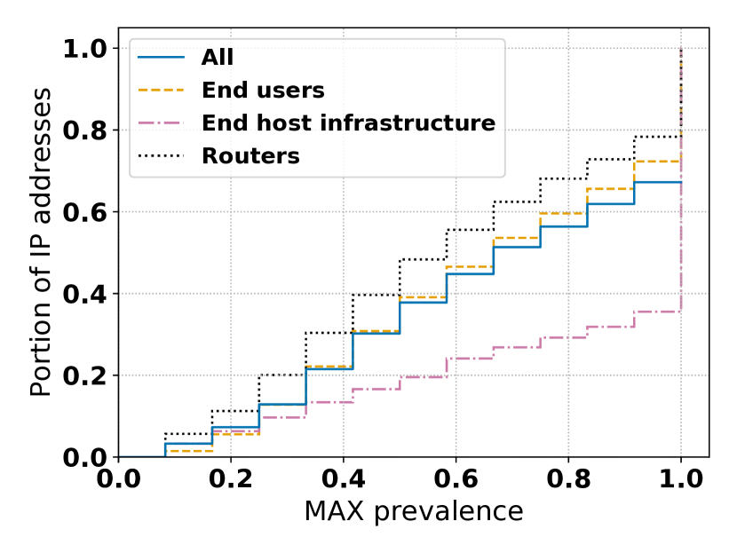
(b) By IP class (Eq. 6)

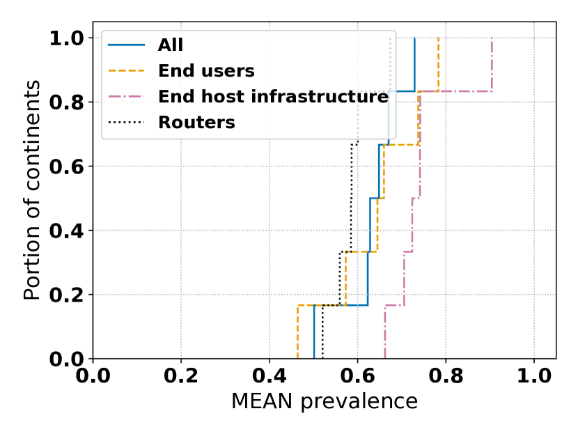
(c) By continent (Eq. 8)

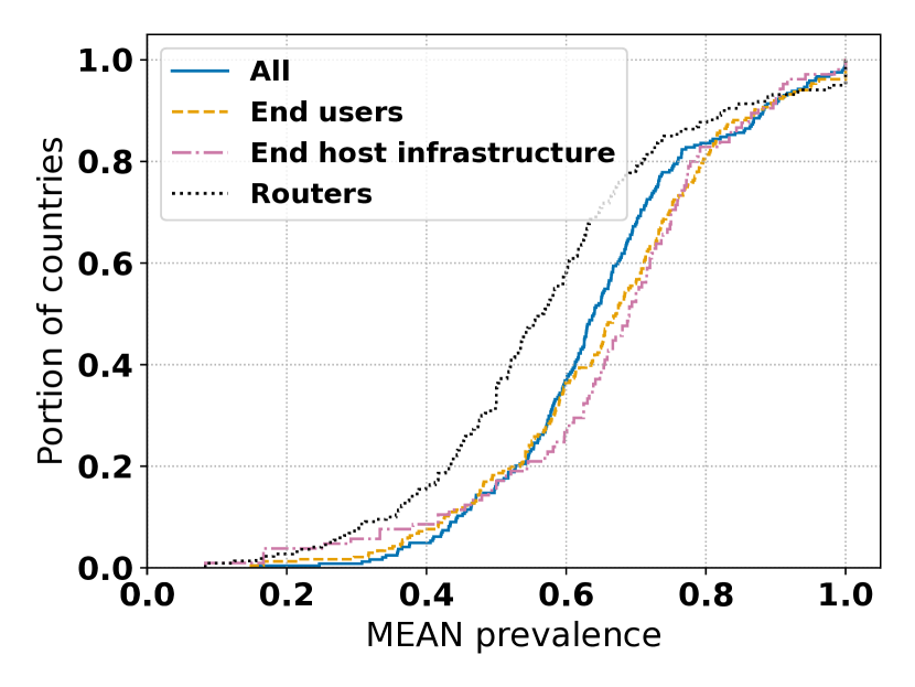
(d) By country (Eq. 8)

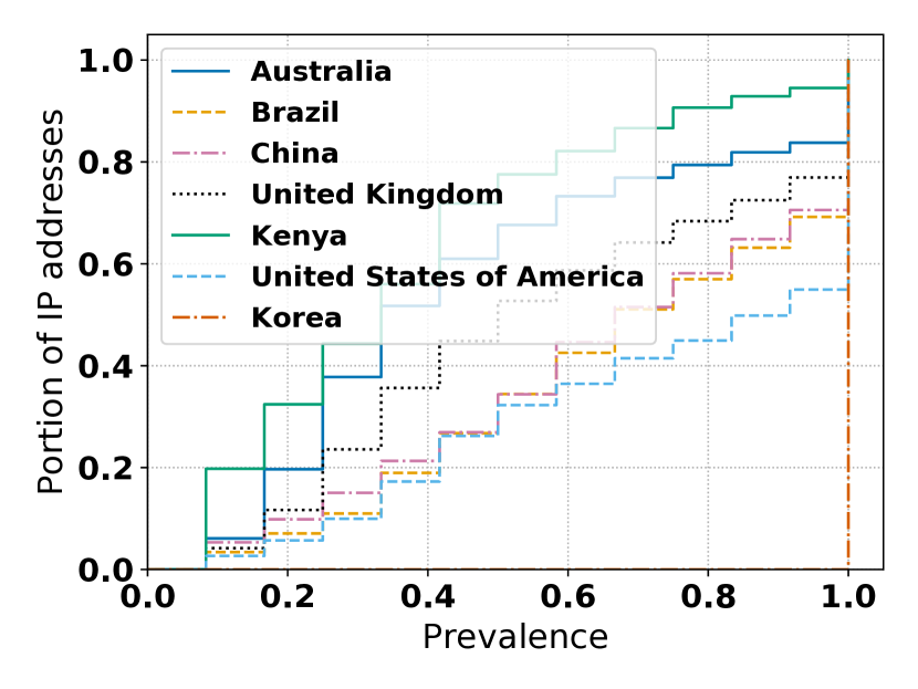
(e) All (Eq. 7)

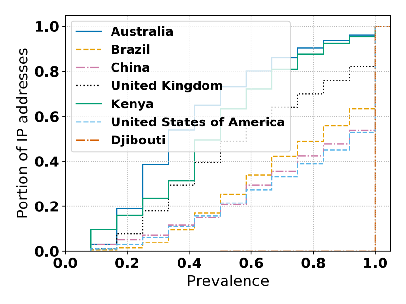
(f) End users (Eq. 7)

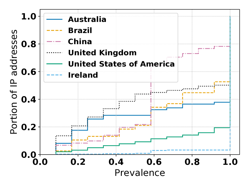
(g) End host infra. (Eq. 7)

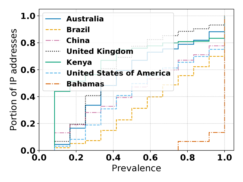
(h) Routers (Eq. 7)

Figure 11. Prevalence results on MaxMind city geolocation

B.1. Prevalence on MaxMind city database

Fig. 11 shows our results on the prevalence for the MaxMind city database. We evaluate the prevalence on cities with the same methodology as we did for the MaxMind country database on our three axes.

Evolution of the prevalence, Fig. 11(a), Eq. 6

First of all, we observe that the shape of the distributions are totally different compared to the MaxMind country database. They are not concentrated near 1. This means that most IP addresses do not have a single dominant city.

Regarding the maximum prevalence over time, we do not identify any trend, except that we can notice that the two last years 2018 and 2019 have their curves of their distributions above the others, meaning that IP addresses tend to not have a dominant city even more for these two years.

Per type of IP addresses, Fig. 11(b), Eq. 6

We notice a clear difference between end host infrastructure and the others; they have a higher maximum prevalence, but still, 20% of the IP addresses have a maximum prevalence of 0.5, meaning that they do not have a single city, or even a highly dominant one.

Per geographical locations, Fig. 11(c) and 11(d), Eq. 8

We observe that the average prevalence depends on the continent: If we take extreme values for all curves, it goes from 0.45 to 0.9.

At country level, the range of average prevalence goes from 0.08 to almost 1, with a median between 0.54 and 0.70 depending on the type of IP addresses. This means that the prevalence on cities is highly dependent on the country.

Like we did for MaxMind country database, we further investigate these differences.

Detailed investigation on continents, second row of Fig. 11, Eq. 7

We see that for all continent and for all types of IP addresses, the range of possibles maximum prevalence goes from almost 0.08 to 1. For “all”, end users, and end host infrastructure, North America has the highest prevalence in general, while for routers, South America has the highest prevalence.

Detailed investigation on countries, third row of Fig. 11, Eq. 7

This time, for each type of IP address, we show the the 10 countries having, this time, the highest average prevalence (Eq. 8). There are considerable differences depending on the type of IP address. On the “All” dataset, the 10 countries are either countries in Africa or small Islands, with the interesting exception of Korea, which has the highest average prevalence. On end users, we mostly find middle eastern and island countries. On end host infrastructure, the 10 countries include countries from all continents, and are big countries, such as US, Canada, Finally, on routers, we find in the ten countries middle east countries, such as Iran, and Irak, and also small countries located in islands.

(a) Over time (Eq. 10)

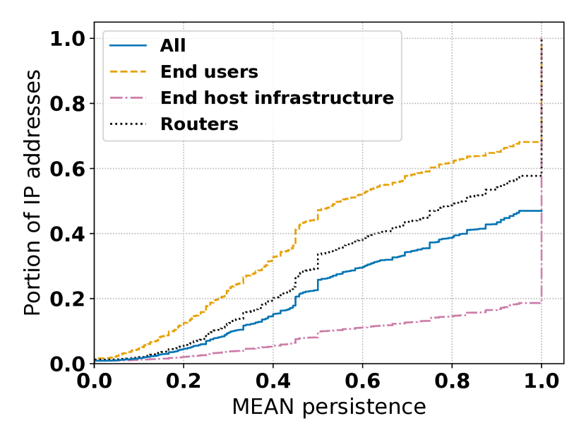
(b) By IP class (Eq. 10)

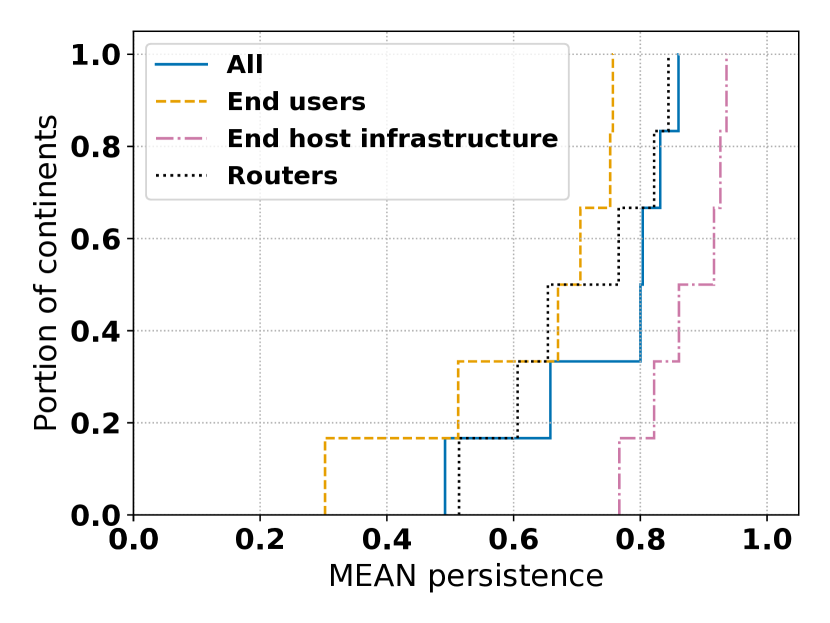
(c) By continent (Eq. 12)

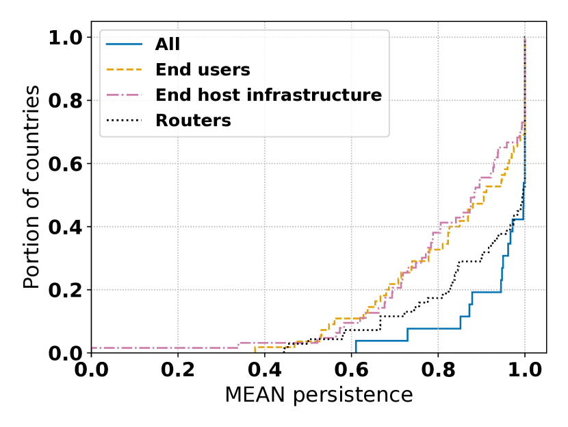
(d) By country (Eq. 12)

(e) All (Eq. 11)

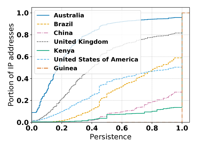
(f) End users (Eq. 11)

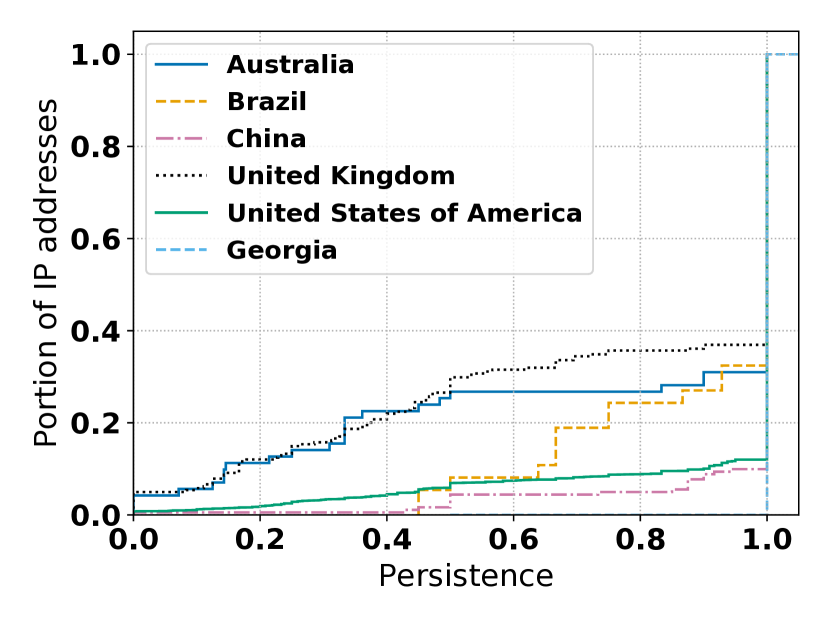
(g) End host infra. (Eq. 11)

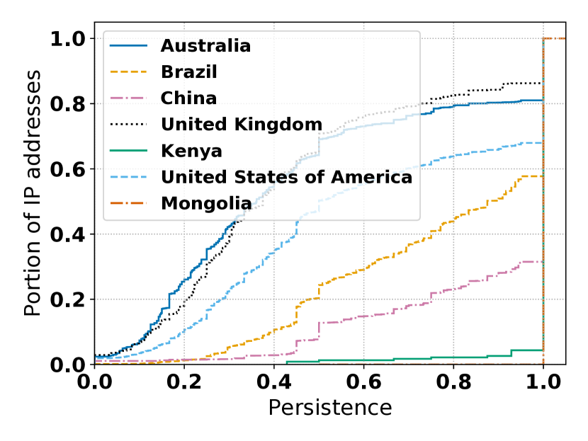
(h) Routers (Eq. 11)

Figure 12. Persistence results on MaxMind city geolocation

B.2. Persistence on MaxMind city database

Evolution of the persistence, Fig. 12(a), Eq. 9

Here is an interesting observation: 2018 and 2019 were the years where the maximum prevalence per IP address were the lower. However, if 2019 is a year where the average persistence is low compared to ohter years (except 2012), 2018 does not have a low average persistence. This shows two things: an IP address can have a low maximum prevalence but a not so low average persistence; city changes in 2018 were rather long term chances compared to 2019.

Per type of IP addresses, Fig. 12(b), Eq. 9

This graphs follows the one on prevalence, with end host infrastructure having a higher average persistence than end users and routers.

Per geographic location, Fig. 12(c) and 12(d), Eq. 12

Here we observe that the average persistence of a location highly depends on the continent and the country. The range of average persistence goes from 0.30 to 0.90, while it goes from 0 to 1 for countries, depending on the type of IP addresses.

Detailed investigation on continents, second row of Fig. 12, Eq. 11

These curves reveals that on all graphs, the curves of Oceania are mostly above the other continents, meaning that the persistence is below the other continents. The order of the other continent depend on the type of IP addresses. Notice that Africa is among the higher persistence for the three types of IP addresses.

Detailed investigation on country, third row of Fig. 12, Eq. 11

Here again, we choose to show the countries having the higher average persistence. The first statement that we make is that even for countries having the higher average persistence, they are not all one concentrated near 1: some IP addresses have short city change, and some other have long.

We notice interesting differences with the graphs on prevalence: For end users, all the countries, except United Kingdom, are countries in Africa, meaning that an IP address having a city change in these countries is more likely to last than in others. For routers, we also find totally difference countries than the ones on prevalence; they are mostly European countries, with US and Saudi Arabia added.

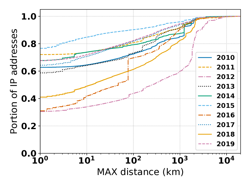
(a) Over time (Eq. 13)

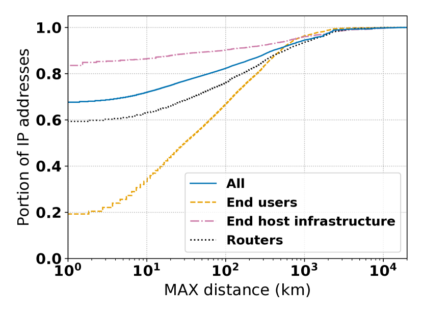
(b) By IP class (Eq. 13)

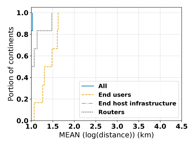
(c) By continent (Eq. 16)

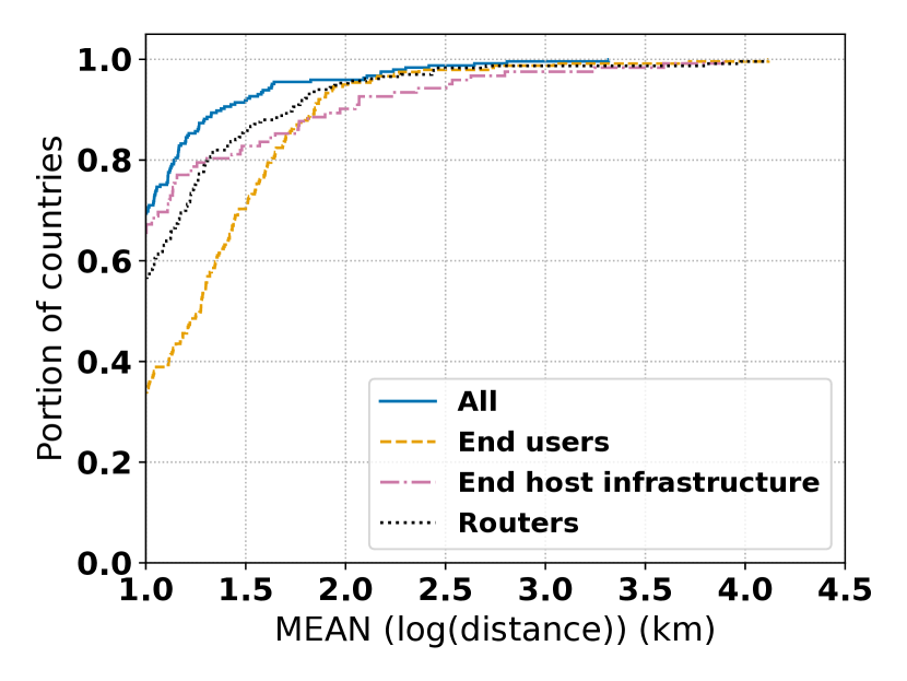
(d) By country (Eq. 16)

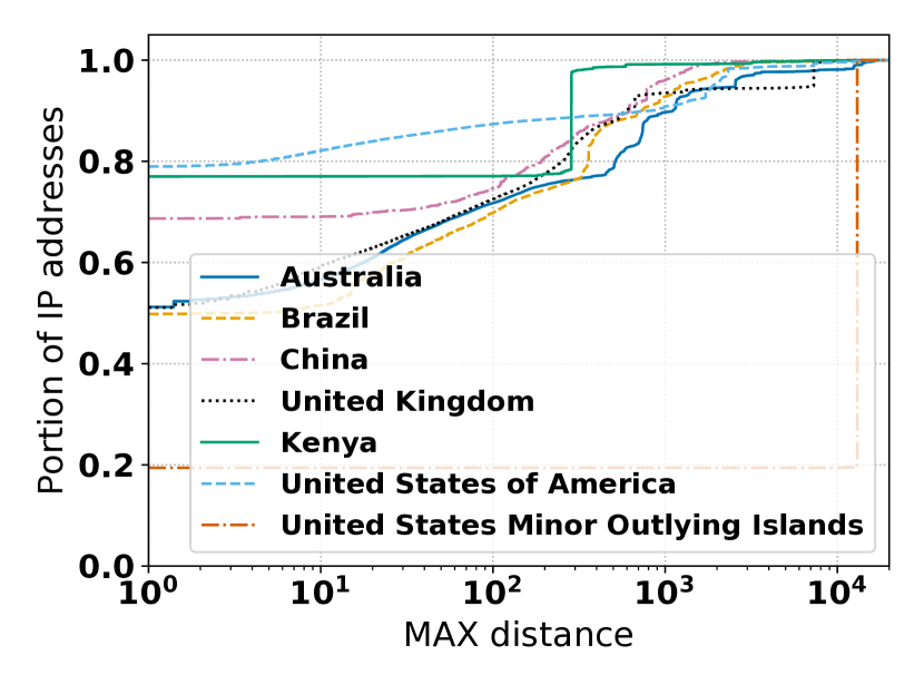
(e) All (Eq. 15)

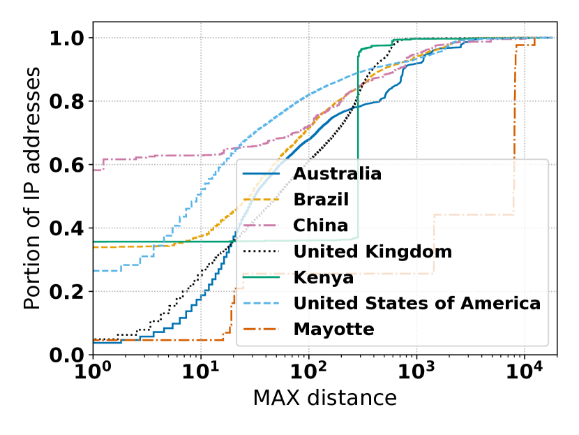
(f) End users (Eq. 15)

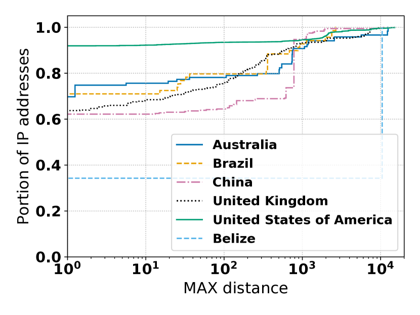
(g) End host infra. (Eq. 15)

(h) Routers (Eq. 15)

Figure 13. Distance results on MaxMind coordinates

Evolution over time (Fig. 13(a), Eq. 13)

We can observe that there is a lot of variations across years. Indeed there are from 10% (in 2015) to 57% of IP addresses (in 2012) that had a maximum distance of more than 100 KM.

Per type of IP addresses (Fig. 13(b), Eq. 13)

Again, the maximum distance depends on the type of IP address. End users have the greater portion of IP addresses experiencing a maximum distance of more than 100 KM (35%), whereas end host infrastructure have 10%. Notice also for all type of IP addresses, few IP addresses have a ¿ 1000 KM maximum distance (6% at most).

Per geographic location (Fig. 13(c) and 13(d), Eq. 16)

Recall that our metric represents, per location, the average of the maximum logarithmic distance between two pairs of coordinates of an IP address where at least one is in the continent or the country.

First of all, we see that this metric for continents is rather small. It goes from value near one (¡ 10 km), to a value of 1.6 (39 km). But on countries, like for prevalence, the distribution is more spread, going from less than one to more than 4, which correspond to 10,000 km. We detail this distribution in the next paragraphs.

Detailed investigation on continents (second row of Fig. 13, Eq. 15)

In general, on all four graphs, whatever the continent, there are a significant portion of IP addresses that have a maximum distance between two of their locations of more than 100 KM. We can also observe that the maximum distance in continents depend on the type of IP address; North America is have statistically fewer distance for end users and end host infrastructure, whereas it is Asia for routers.

Detailed investigation on countries (third row of Fig. 13, Eq. 15)

In these graphs, we show the ten countries that have the highest value for the metric defined in Eq. 16, i.e., the countries where the distances are the higher. Again, like for prevalence and persistence, the countries depend on the type of IP address. For end users, they are mainly located in small countries in islands. For end host infrastructure, these are either medium or big countries in all continents (e.g., India, Bulgaria, Argentina). For routers, we find countries in small islands and countries in Africa.

References

- (1)
- max (2019) 2019. Significant Changes to Accessing and Using GeoLite2 Databases. https://blog.maxmind.com/2019/12/18/significant-changes-to-accessing-and-using-geolite2-databases/.
- cai (2020) 2020. Caida ITDK. http://www.caida.org/data/internet-topology-data-kit/index.xml.
- ip2 (2020) 2020. IP2Loc atabase. https://www.ip2location.com.
- mla (2020) 2020. M-Lab public datasets. https://www.measurementlab.net/data/.
- max (2020) 2020. MaxMind. https://www.maxmind.com/en/home.
- net (2020) 2020. NetAcuity database. https://www.digitalelement.com/solutions/.
- rou (2020) 2020. Route Views. http://www.routeviews.org/.
- Akamai (2020) Akamai. 2020. EdgeScape. https://developer.akamai.com/edgescape.
- Anonymous (2020) Anonymous. 2020. Longitudinal Study of an IP Geolocation Database. Technical Report. http://anony.mo.us.
- Antonakakis et al. (2017) Manos Antonakakis, Tim April, Michael Bailey, Matt Bernhard, Elie Bursztein, Jaime Cochran, Zakir Durumeric, J Alex Halderman, Luca Invernizzi, Michalis Kallitsis, et al. 2017. Understanding the Mirai Botnet. In USENIX Security). 1093–1110.
- Cajori (1993) Florian Cajori. 1993. A history of mathematical notations. Vol. 1. Courier Corporation.
- Deng et al. (2017) Jie Deng, Gareth Tyson, Felix Cuadrado, and Steve Uhlig. 2017. Internet scale user-generated live video streaming: The Twitch case. In PAM. Springer, 60–71.
- Eriksson et al. (2010) Brian Eriksson, Paul Barford, Joel Sommers, and Robert Nowak. 2010. A learning-based approach for IP geolocation. In PAM. Springer, 171–180.
- Gharaibeh et al. (2017) Manaf Gharaibeh, Anant Shah, Bradley Huffaker, Han Zhang, Roya Ensafi, and Christos Papadopoulos. 2017. A look at router geolocation in public and commercial databases. In Proc. ACM IMC. 463–469.
- Gueye et al. (2006) Bamba Gueye, Artur Ziviani, Mark Crovella, and Serge Fdida. 2006. Constraint-based geolocation of internet hosts. IEEE/ACM Transactions on Networking 14, 6 (2006), 1219–1232.
- Hexasoft (2020) Hexasoft. 2020. IP2Location. https://www.ip2location.com.
- Huffaker et al. (2014) Bradley Huffaker, Marina Fomenkov, et al. 2014. DRoP: DNS-based Router Positioning. ACM SIGCOMM Computer Communication Review 44, 3 (2014), 5–13.
- Huffaker et al. (2011) Bradley Huffaker, Marina Fomenkov, and K Claffy. 2011. Geocompare: A Comparison of Public and Commercial Geolocation Databases. Proc. NMMC, 1–12.
- Katz-Bassett et al. (2006) Ethan Katz-Bassett, John P John, Arvind Krishnamurthy, David Wetherall, Thomas Anderson, and Yatin Chawathe. 2006. Towards IP geolocation using delay and topology measurements. In Proc. ACM SIGCOMM. 71–84.
- Kline et al. (2020) E. Kline, K. Duleba, Z. Szamonek, S. Moser, and W. Kumari. 2020. A Format for Self-published IP Geolocation Feeds. IETF Draft. https://tools.ietf.org/html/draft-google-self-published-geofeeds-09
- Komosnỳ et al. (2017) Dan Komosnỳ, Miroslav Vozňák, and Saeed Ur Rehman. 2017. Location accuracy of commercial IP address geolocation databases. (2017).
- Kotronis et al. (2017) Vasileios Kotronis, George Nomikos, Lefteris Manassakis, Dimitris Mavrommatis, and Xenofontas Dimitropoulos. 2017. Shortcuts through colocation facilities. In Proc. ACM IMC. 470–476.
- Lee and Spring (2016) Youndo Lee and Neil Spring. 2016. Identifying and aggregating homogeneous ipv4/24 blocks with hobbit. In Proc. ACM IMC. 151–165.
- Lilliefors (1967) Hubert W Lilliefors. 1967. On the Kolmogorov-Smirnov test for normality with mean and variance unknown. Journal of the American statistical Association 62, 318 (1967), 399–402.
- Padmanabhan et al. (2019) Ramakrishna Padmanabhan, Aaron Schulman, Dave Levin, and Neil Spring. 2019. Residential links under the weather. In Proc. SIGCOMM. 145–158.
- Padmanabhan and Subramanian (2001) Venkata N. Padmanabhan and Lakshminarayanan Subramanian. 2001. An Investigation of Geographic Mapping Techniques for Internet Hosts. In Proc. ACM SIGCOMM (San Diego, California, USA) (SIGCOMM). Association for Computing Machinery, New York, NY, USA, 173–185. https://doi.org/10.1145/383059.383073
- Papadopoulos et al. (2017) Panagiotis Papadopoulos, Nicolas Kourtellis, Pablo Rodriguez Rodriguez, and Nikolaos Laoutaris. 2017. If you are not paying for it, you are the product: How much do advertisers pay to reach you?. In Proc. ACM IMC. 142–156.
- Paxson (1997) Vern Paxson. 1997. End-to-end routing behavior in the Internet. IEEE/ACM Transactions on Networking 5, 5 (1997), 601–615.
- Paxson (2004) Vern Paxson. 2004. Strategies for Sound Internet Measurement. In Proceedings of the 4th ACM SIGCOMM Conference on Internet Measurement (Taormina, Sicily, Italy) (IMC ’04). Association for Computing Machinery, New York, NY, USA, 263–271. https://doi.org/10.1145/1028788.1028824
- Pearce et al. (2017) Paul Pearce, Ben Jones, Frank Li, Roya Ensafi, Nick Feamster, Nick Weaver, and Vern Paxson. 2017. Global Measurement of DNS Manipulation. In USENIX Security). 307–323.
- Poese et al. (2011) Ingmar Poese, Steve Uhlig, Mohamed Ali Kaafar, Benoit Donnet, and Bamba Gueye. 2011. IP Geolocation Databases: Unreliable? ACM SIGCOMM Computer Communication Review 41, 2 (2011), 53–56.
- Scheitle et al. (2018) Quirin Scheitle, Oliver Hohlfeld, Julien Gamba, Jonas Jelten, Torsten Zimmermann, Stephen D. Strowes, and Narseo Vallina-Rodriguez. 2018. A Long Way to the Top: Significance, Structure, and Stability of Internet Top Lists. In Proc. ACM IMC (Boston, MA, USA). New York, NY, USA, 478–493. https://doi.org/10.1145/3278532.3278574
- Shavitt and Zilberman (2011) Yuval Shavitt and Noa Zilberman. 2011. A geolocation databases study. IEEE Journal on Selected Areas in Communications 29, 10 (2011), 2044–2056.
- Sklower (1991) Keith Sklower. 1991. A tree-based packet routing table for Berkeley unix.. In USENIX Winter, Vol. 1991. 93–99.
- Vermeulen et al. (2020) Kevin Vermeulen, Justin P Rohrer, Robert Beverly, Olivier Fourmaux, and Timur Friedman. 2020. Diamond-Miner: Comprehensive Discovery of the Internet’s Topology Diamonds. In USENIX NSDI. 479–493.
- Wang et al. (2011) Yong Wang, Daniel Burgener, Marcel Flores, Aleksandar Kuzmanovic, and Cheng Huang. 2011. Towards Street-Level Client-Independent IP Geolocation. In USENIX NSDI, Vol. 11. 27–27.
- Weinberg et al. (2018) Zachary Weinberg, Shinyoung Cho, Nicolas Christin, Vyas Sekar, and Phillipa Gill. 2018. How to catch when proxies lie: Verifying the physical locations of network proxies with active geolocation. In Proc. IMC. 203–217.
- Winter et al. (2019) Philipp Winter, Ramakrishna Padmanabhan, Alistair King, and Alberto Dainotti. 2019. Geo-locating BGP prefixes. In IEEE TMA. 9–16.