On the Selection of Loss Severity Distributions to Model Operational Risk

Abstract

Accurate modeling of operational risk is important for a bank and the finance industry as a whole to prepare for potentially catastrophic losses. One approach to modeling operational is the loss distribution approach, which requires a bank to group operational losses into risk categories and select a loss frequency and severity distribution for each category. This approach estimates the annual operational loss distribution, and a bank must set aside capital, called regulatory capital, equal to the 99.9% quantile of this estimated distribution. In practice, this approach may produce unstable regulatory capital calculations from year-to-year as selected loss severity distribution families change. This paper presents truncation probability estimates for loss severity data and a consistent quantile scoring function on annual loss data as useful severity distribution selection criteria that may lead to more stable regulatory capital. Additionally, the Sinh-arcSinh distribution is another flexible candidate family for modeling loss severities that can be easily estimated using the maximum likelihood approach. Finally, we recommend that loss frequencies below the minimum reporting threshold be collected so that loss severity data can be treated as censored data.

Keywords: operational risk, advanced measurement approach, loss distribution approach, regulatory capital

1 Introduction

The Basel Committee on Banking Supervision (BCBS) defines operational risk (OR) in the second Basel accords (Basel II) as

“the risk of a loss resulting from inadequate or failed internal processes, people and systems, or from external events. This definition includes legal risk but excludes strategic and reputational risk.” (BCBS,, 2006)

To mitigate potential operational losses, regulators require that a bank set aside a minimum amount of capital for one year called regulatory capital (RC).

The advanced measurement approach (AMA) presented in Basel II calculates RC as the $99.9\%$ quantile of the estimated firm-wide annual operational loss distribution. This distribution is commonly estimated using the loss distribution approach (LDA), which requires a bank to estimate and select the loss frequency and loss severity distributions for each regulatory risk category (RRC) and treat firm-wide annual operational loss as a compound sum of the annual losses from each RRC.

A major obstacle facing banks using the AMA is to develop a procedure that provides stable RC calculations year-to-year. Large increases in RC that result from poor modeling procedures require the bank to set aside more assets that cannot be used freely to generate revenue, so a bank has an intrinsic interest in minimizing the probability of overestimating RC. Regulators scrutinize large decreases in a bank’s RC, so a bank may also face problems in subsequent years when the overestimation is corrected. Stability in RC is a common problem faced by industry that is not well covered in the operational risk literature.

Loss frequencies for a given RRC tend to follow predictable patterns, so the instability in RC is primarily generated by the loss severity distribution selection process. A popular selection process uses a list of candidate severity distribution families, estimates each distribution using historical operational loss data, and selects the “best” distribution based on some criteria. When a RRC’s selected severity distribution changes families from one year to the next, that RRC’s contribution to firm-wide annual operational loss is likely to change dramatically. For this reason, we are interested in finding a flexible distribution family that can outperform other candidates year-after-year.

Operational loss data usually exhibit extreme positive-skew and can have various right-tail behaviors. The log transform of operational loss severities, called log-losses, also exhibit positive skew. As a result, candidate distribution families should be able to fit loss or log-loss data that is asymmetric with various tail behaviors. Two-parameter distribution families, while popular in industry and easy to estimate, are not flexible enough to accomplish both goals. Spliced and mixture distributions are flexible enough to fit asymmetric, right-skewed data, but require the estimation of additional parameters for splicing points or component proportions. The four-parameter $g$-and-$h$ distribution (GNH) (Hoaglin,, 1985; Dutta and Perry,, 2006; Degen et al.,, 2007) is a flexible distribution family sometimes used to model loss severities, but presents challenges when estimated by maximum likelihood estimation (MLE). The Sinh-arcSinh distribution (SAS) (Jones and Pewsey,, 2009) provides us with a flexible four-parameter candidate distribution family that is able to accurately fit log-loss severity data for many RRC’s. By treating loss severities as the exponential transformation of a SAS random variable, we introduce the log-Sinh-arcSinh distribution (LSAS) as a viable loss severity candidate distribution family. LSAS maintains the flexibility of GNH, but is easier work with numerically.

For each RRC, we estimate each candidate severity distribution family using historical data of operational losses from that RRC. Historical loss data are truncated, so the data are comprised of only those losses exceeding a known minimum reporting threshold. For each candidate severity distribution family, MLE is used to estimate the parameters. Finally, one severity distribution is selected from the estimated candidate distributions. This paper is primarily focused with the selection process.

Severity distributions are commonly evaluated by performance measures inspired by the five listed in Dutta and Perry, (2006). Hypothesis tests for appropriate severity distributions include Kolmogorov-Smirnov and Anderson-Darling. Through simulation, we found that these tests have low power and tend to include too many inappropriate distributions. Relative measures of fit may include Akaike’s Information Criterion (AIC) (Akaike,, 1974) and Bayesian Information Criterion (BIC) (Schwarz,, 1978), however neither criterion can tell us if any distribution is a good fit. Dutta and Perry, (2006) consider a severity distribution “realistic” if it produces regulator capital no more than 3% of a bank’s assets. However, this criterion is applied to RC and cannot be immediately applied to each RRC.

We consider two additional severity distribution selection criteria that can be applied to each RRC, the truncation probability estimate and the quantile scoring function (QS) (Gneiting,, 2011). Details for our selection criteria are given in Section 3.4. When estimating a distribution family from left-truncated data with a known truncation point, evaluating the cumulative distribution function (CDF) at the truncation point given the estimated parameters produces an estimate of the proportion of losses that occur below this threshold. Thus, we can consider a candidate severity distribution “realistic” if its truncation probability estimate is reasonable. We take a rather conservative stance and consider any truncation probability estimate less than 50% to be reasonable. This criterion can be applied to each RRC independently, making it particularly useful for the LDA. To better understand the range of reasonable truncation probability estimates, we promote the collection of loss frequencies below the truncation point. We present improved truncation probability estimates when using censored data in Section 5.3 to motivate the collection of all loss frequencies.

The second criterion, the QS, uses a consistent scoring function to evaluate forecasts. Since Basel II defines RC as the forecasted 99.9% quantile of the estimated firm-wide annual loss distribution, the performance of an OR modeling procedure should be measured by its ability to predict the extreme right-tail of this distribution. Under the assumption of weak dependence between the annual losses of each RRC, the sum of the 99.9% quantile of each RRC’s estimated annual loss distribution can be used as a proxy for RC. Thus, we can evaluate the QS on the annual losses for each RRC and select the severity distribution with the best (lowest) score. The QS criterion is used in our simulation study in Section 5.4 to rank loss severity distributions and consistently favors appropriate distributions.

The struggle of financial institutions to produce stable RC calculations could be a contributing factor in the decision by BCBS to move away from the AMA. In the next manifestation of the Basel accords, Basel III, the AMA is being removed from the regulatory framework.

“The option to use an internal model-based approach for measuring operational risk - the ‘Advanced Measurement Approaches’ (AMA) - has been removed from the operational risk framework. BCBS believes that modeling of operational risk for regulatory capital purposes is unduly complex and that the AMA has resulted in excessive variability in risk-weighted assets and insufficient levels of capital for some banks.” (BCBS,, 2016)

Despite this proposed change in regulations, a bank still has plenty of motivation to use the AMA for internal modeling of their OR. According to the article, “The Final Bill - financial crime” (Economist,, 2016), there have been 188 settlements from 2009 to August 2016 for criminal and civil prosecutions against banks costing $219 billion. Eleven firms have paid penalties in excess of 10% of their market capitalization. In March 2018, Barclays was ordered to pay $2 billion in civil penalties for fraudulently selling mortgage securities that contributed to the 2008 financial crisis and in April 2018, Wells Fargo was fined $1 billion for the “bank’s failures to catch and prevent problems, including improper charges to consumers in its mortgage and auto-lending businesses.” (Strasburg, 2018; Hayashi, 2018).

In Section 2, we briefly review the LDA. Our severity distribution estimation and selection process is presented in Section 3, while Section 4 illustrates the importance of the truncation probability estimate on the loss frequency and its role in estimating the annual loss distribution. A simulation study is performed in Section 5 that portrays the instability of RC when selecting a severity distribution based on AIC and the modified Anderson-Darling test, compares the GNH and LSAS distribution families, examines improvements to truncation probability estimation when using censored data, and gauges the performance of selecting the severity distribution from the QS on annual loss data. All simulations and numerical analyses use the R software available at https://www.r-project.org/. Section 6 summarizes our conclusions and suggests areas for future research.

2 Loss Distribution Approach

Under the Basel II AMA guidelines, operational loss events are partitioned into eight business lines and seven event types. When an operational loss occurs, it is mapped to one of 56 business line/event type intersections, called a regulatory risk category (RRC). This mapping process is further explained in BCBS, (2006). Each loss event must be assigned a time stamp, a loss amount, and a RRC. The time stamp is usually a fiscal quarter or year and the loss amount is a positive value. The number of loss events that occur in a particular RRC over a given time period is called the loss frequency, and each loss amount is called the loss severity.

Historical loss data are used to estimate the loss frequency and severity distributions by interpreting the historical loss data as realizations of random variables. Under an AMA, the historical loss data should reflect all current, material activities, risk exposures, and loss events whose loss severities exceed a minimum threshold. For example, a bank that sells off or discontinues a business line should no longer use those losses in their AMA. Using notation adapted from Embrechts and Hofert, (2011), loss events are denoted as

$$\big{\{}X_{t,n}^{b,l}\big{\}},\quad\text{for $t=1,2,...,T$; $b=1,2,...,8$; $l=1,2,...,7$; $n=1,2,...,N_{t}^{b,l}$},$$ (1)

where $X_{t,n}^{b,l}$ is a random variable for the loss severity of the $n^{\text{th}}$ loss event occurring in fiscal year $t$ for business line $b$ and event type $l$, and $N_{t}^{b,l}$ is a random variable for the number of losses occurring in fiscal year $t$ for business line $b$ and event type $l$. Thus, $S_{T+1}$ is a random variable for firm-wide annual operational loss for next fiscal year and can be calculated as

$$S_{T+1}=\sum_{b=1}^{8}\sum_{l=1}^{7}\sum_{n=1}^{N^{b,l}_{T+1}}X_{T+1,n}^{b,l}=\sum_{b=1}^{8}\sum_{l=1}^{7}L^{b,l}_{T+1},$$ (2)

where $L^{b,l}_{T+1}$ is the annual loss for business line $b$ and event type $l$ in year $T+1$. The goal of the LDA is to estimate the distribution of $S_{T+1}$ via simulation and calculate RC as the 99.9% quantile of this estimated distribution.

There are two sources of randomness in $S_{T+1}$, the loss frequency and the loss severity. The loss frequency, $N_{T+1}^{b,l}$, is a discrete random variable for the number of losses occurring next fiscal year in business line $b$ and event type $l$. The loss severity, $X_{T+1,n}^{b,l}$, is a non-negative, continuous random variable as defined in (1). When calculating RC, we follow two common assumptions:

• $N_{t}^{b,l}$, are independent of $X_{t,n}^{b,l}$ for a given business line $b$, event type $l$, and year $t$;

• $\{X_{t,n}^{b,l}\}_{t=1,2,\dots;\ n=1,2,\dots,N_{t}^{b,l}}$ are independent and identically distributed for a given business line $b$ and event type $l$.

For the purpose of estimating loss severity distributions, losses mapped to a given event type may be combined across business lines to produce an operational risk category (ORC), which is the level at which the bank’s model generates a separate distribution to estimate potential losses (BCBS,, 2011). We assume an annual loss frequency with no trend. A general solution to modeling trends in the loss frequency is presented in Chavez-Demoulin et al., (2015). These simplifying assumptions help us avoid complexities that do not contribute to the understanding of loss severity distribution selection. Since RC is an annual forecast, the use of an annual loss frequency mitigates both structural reporting bias and temporal clustering of losses that were evidenced by the 2004 Loss Data Collection Exercise (LDCE) (Dutta and Perry,, 2006). By assuming no trend, we can assume annual loss frequencies are independent and identically distributed for each ORC. Finally, working with ORC loss frequencies allows us to disregard how frequencies are combined across RRC’s and simplifies our notation. Letting $r$ represent a specific ORC, loss events can be rewritten from Equation (1) as

$$\big{\{}X_{t,n}^{r}\big{\}},\quad\text{for $t=1,2,...,T$; $r=1,2,...,R$; $n=1,2,...,N_{t}^{r}$},$$

and the firm-wide annual operational loss from Equation (2) becomes

$$S_{T+1}=\sum_{r=1}^{R}\sum_{n=1}^{N^{r}_{T+1}}X_{T+1,n}^{r}=\sum_{r=1}^{R}L^{r}_{T+1}.$$ (3)

When internal data is too sparse for an ORC, Basel II allows a banks’ internal data to be supplemented by an external database. Some external datasets include losses from banks of various sizes located all over the world. Hence, care should be taken to filter the data so that they are appropriate in size and scope. Additionally, an external database may have a minimum reporting threshold for loss data collection that differs from a bank’s. If external data are used to supplement internal data, the higher of the bank’s and database’s reporting threshold may need to be applied to all data for that ORC. Since some ORC’s may be supplemented by external data and others may not, a bank can have different minimum reporting thresholds for different ORC’s.

3 Loss Severity Estimation and Selection

Regulations require that a bank’s internal operational loss data include all loss events whose severities exceed a minimum threshold, so we assume that we have no information about the loss events that occur below the threshold. As a result, the datasets are treated as left-truncated. In Section 5.3, we investigate the impact of data collection for the loss frequency below the reporting threshold by comparing truncation probability estimates to censored probability estimates. The remainder of this section includes an overview of the truncation and censoring approaches, presents candidate severity distributions, and introduces our severity distribution selection criteria.

3.1 Truncation Approach

The truncation approach assumes that losses below the minimum threshold belong to the same distribution as the losses above the threshold. In order to use the MLE approach on truncated datasets to estimate the loss severity distributions, we must derive the likelihood function from the conditional density given the truncation point. For $n$ loss events exceeding the minimum threshold in a given ORC, assume loss amounts $X_{1},X_{2},...,X_{n}\ \stackrel{{\scriptstyle iid}}{{\mathrm{\sim}}}\ F$, where $F$ is some loss severity distribution with parameters $\bm{\theta}\in\bm{\Theta}$. If we let $\tau$ represent the non-random minimum reporting threshold of the given ORC, then given the truncation point $tau$, the conditional CDF for a reported loss is

$$\widetilde{F}(x;\bm{\theta},\tau)=\frac{F(x;\bm{\theta})-F(\tau;\bm{\theta})}{1-F(\tau;\bm{\theta})}.$$

The conditional probability density function (PDF) for a reported loss is

$$\tilde{f}(x;\bm{\theta},\tau)=\frac{d}{dx}\widetilde{F}(x;\bm{\theta},\tau)=\frac{f(x;\bm{\theta})}{1-F(\tau;\bm{\theta})}.$$

We can estimate $\bm{\theta}$ via MLE on a sample, $\mathbf{x}$, using the likelihood function

$$\widetilde{L}(\bm{\theta};\mathbf{x},\tau)=\prod_{i=1}^{n}\ \tilde{f}(x_{i};\bm{\theta},\tau)=\big{[}1-F(\tau;\bm{\theta})\big{]}^{-n}\prod_{i=1}^{n}f(x_{i};\bm{\theta}),$$ (4)

by maximizing $\widetilde{L}(\bm{\theta};\mathbf{x},\tau)$ over all $\bm{\theta}\in\bm{\Theta}$. The MLE is denoted $\widehat{\bm{\theta}}$.

The truncation probability is the probability that a loss event occurs but does not exceed the minimum threshold and is estimated by $F(\tau;\widehat{\bm{\theta}})$. When estimating the annual loss distribution, we simulate losses from the unconditional severity distribution to account for the downward bias of treating a truncated sample as complete (Baud et al.,, 2003; Chernobai et al.,, 2005; Luo et al.,, 2007).

3.2 Censoring Approach

When estimating the candidate distribution families using the truncation approach, each distribution has a truncation probability estimate. When loss severity data are generated by a process with regularly varying (RV) tail behavior, the truncation probability estimates produced by distribution families with subexponential (SUBEX) tail behavior can become unreasonably ($>50\%$) large (Perline,, 2005). Without data collection or expert opinion for the frequency of losses below a reporting threshold, however, it can be challenging to decide a reasonable range of values for the truncation probability. To encourage banks to start collecting the frequency of losses below the reporting threshold, we compare the truncation probabilities estimated from datasets truncated at $\tau$ to the censored probabilities estimated from the same datasets censored at $\tau$. The results of our simulation, presented in Section 5.3, make a compelling argument that this additional data collection may be worthwhile.

Similar to the truncation approach, the censoring approach also assumes losses above and below the reporting threshold follow the same distribution. To derive the likelihood function, assume loss severities are a sequence of random variables, $X_{1},X_{2},...,X_{n}\ \stackrel{{\scriptstyle iid}}{{\mathrm{\sim}}}\ F$, for some loss severity distribution $F$ with parameters $\bm{\theta}\in\bm{\Theta}$. Let $\tau$ represent the non-random minimum reporting threshold. Then, let $Y_{i}=\max(\tau,X_{i})$ and $Y_{i_{1}},Y_{i_{2}},\dots,Y_{i_{m}}>\tau$ with $0\leq m\leq n$, so that we have full loss severity data for $m$ of the $n$ loss events. The likelihood function for censored data is

$$\widetilde{L}_{c}(\bm{\theta};\mathbf{x},\tau)=\big{[}F(\tau;\bm{\theta})\big{]}^{n-m}\ \prod_{i\in I_{m}}f(x_{i};\bm{\theta}),$$ (5)

where $I_{m}=\{i=1,2,\dots,n:X_{i}>\tau\}$. By maximizing $\widetilde{L}_{c}(\bm{\theta};\mathbf{x},\tau)$ over all $\bm{\theta}\in\bm{\Theta}$, we find the MLE, $\widehat{\bm{\theta}}_{c}$. The censoring probability estimate is calculated as $F(\tau;\widehat{\bm{\theta}}_{c})$.

3.3 Candidate Distributions

For each ORC, we assume that loss severities are generated from one of the following parametric distributions: lognormal distribution (LGN), generalized Pareto distribution (GPD), Burr distribution (BUR), Weibull distribution (WBL), Loglogistic distribution (LLOG), GNH, LSAS, lognormal body spliced with lognormal tail (LGNLGN), and lognormal body spliced with generalized Pareto tail (LGNGPD). Each distribution is able to capture the salient properties of unimodality and asymmetry typically exhibited by operational loss data. There are many references that contain candidate loss severity distributions including Chernobai et al., (2007), Panjer, (2006), and Peters and Shevchenko, (2015).

We briefly define both GNH and LSAS and give their distribution function. Let $Z\sim N(0,1)$. Then,

$$X=a+b\cdot A_{g,h}(Z)=a+b\ \Big{(}\frac{e^{gZ}-1}{g}\Big{)}e^{hZ^{2}/2},$$

is said to have a $g$-and-$h$ distribution (Hoaglin,, 1985) where $a\in\mathbb{R}$ is a location parameter and $b>0$ is a scale parameter. To ensure monotonicity of the $g$-and-$h$ transformation, $A_{g,h}(\cdot)$, we further assume $g\in\mathbb{R}$ and $h>0$ for the skewness and elongation parameters, respectively. As shown by Degen et al., (2007), these restrictions impose a RV right-tail on GNH with index $-1/h$. Thus, we lose the ability to model SUBEX and superexponential (SUPEX) tail behaviors.

The LSAS distribution is the result of an exponential transformation of a Sinh-arcSinh (Jones and Pewsey,, 2009) random variable. It is a four-parameter generalization of the two-parameter lognormal distribution with two additional parameters that allow for more flexible skewness and tailweight. Let $Z\sim N(0,1)$. Then,

$${Y=a+b\cdot A_{\epsilon,\delta}(Z)=a+b\ \sinh\Big{\{}\frac{\sinh^{-1}(Z)+\epsilon}{\delta}\Big{\}}},$$

is said to have a Sinh-arcSinh distribution with location parameter $a\in\mathbb{R}$, scale parameter $b>0$, skewness parameter $\epsilon\in\mathbb{R}$, and tailweight parameter $\delta>0$. The sinh-arcsinh transformation, $A_{\epsilon,\delta}(\cdot)$, is monotonic over the entire parameter space with a closed-form inverse. Finally, we say that $X=e^{Y}$ has a LSAS distribution.

Unlike GNH, LSAS is able to model RV, SUBEX, and SUPEX right-tail behaviors. Also, the inverse Sinh-arcSinh transformation has a closed-form solution, allowing MLE to run much faster than for GNH, whose inverse transformation requires monotone interpolation of transformed standard normal quantiles for each parameter vector. The LSAS likelihood function has better numerical stability than GNH, because we can calculate the likelihood on the log of the losses. Finally, one should be aware that the support for GNH is $\mathbb{R}$, which allows for negative losses. Simulating losses from the unconditional GNH using the rejection method may overestimate the probability of a large loss. Penalized maximum likelihood can be used to reduce the probability of negative losses, but is not used in our analysis.

3.4 Severity Distribution Selection Criteria

To estimate the candidate severity distributions, we use the MLE approach which is a well established and well respected method of parameter estimation with many desirable optimality properties formalized by Fisher in 1922 (Aldrich,, 1997). Since we employ MLE to estimate each candidate distribution, a natural choice to compare the estimated distributions is AIC (Akaike,, 1974). The AIC is defined as

$$AIC =-2\ \tilde{\ell}(\widehat{\Theta};\mathbf{x},\tau)+2\ k,$$ (6)

where $\tilde{\ell}$ is the log-likelihood function, $\widehat{\Theta}$ is the estimated distribution parameter vector as found via MLE, and $k$ is the number of estimated parameters in the distribution. The number of estimated parameters is included in the AIC to prevent selecting a model that overfits the data. The AIC is a relative performance measure, so while it can compare models, it cannot tell if any model is a good fit. Another weakness of selecting a distribution by AIC is that operational loss severity data are typically skewed with most of the risk lying in the extreme right tail, but AIC is a likelihood measure heavily influenced by the central portion of the data’s distribution. Other diagnostics, such as QQ-plots should be consulted for adequacy of tail fit.

Unlike AIC, the modified Anderson-Darling test (A-D) (Sinclair et al.,, 1990) is a goodness-of-fit test that can be used to eliminate candidate distributions when the data do not follow the estimated distribution with a desired confidence. The modified Anderson-Darling test statistic is calculated as

$$\widehat{AD}=\frac{n}{2}-2\ \sum_{i=1}^{n}\widetilde{F}(x_{(i)};\widehat{\Theta},\tau)-\sum_{i=1}^{n}\Big{[}2-\frac{2i-1}{n}\Big{]}\log\big{[}1-\widetilde{F}(x_{(i)};\widehat{\Theta},\tau)\big{]},$$

where $n$ is the number of observations, $x_{(i)}$ is the $i^{\text{th}}$ order statistic such that $x_{(1)}\leq x_{(2)}\leq\cdots\leq x_{(n)}$, and $\widetilde{F}(x;\widehat{\Theta},\tau)$ is the estimated conditional CDF for the candidate distribution.

The conditional CDF is used to calculate the test statistic, so A-D can often fail to reject distributions with “unreasonable” high truncation probability estimates. This same issue is shared by the Kolmogorov-Smirnov test. As a result, we incorporate the truncation probability estimate into our severity distribution selection process. Under the truncation approach, lighter-tailed distributions can mimic heavy-tailed distributions at sufficiently high truncation levels. For example, Gumbel-type distributions can mimic an inverse power law tail behavior (Perline,, 2005). As a result, high truncation probability estimates can signal which distributions may be inappropriate. From a practical standpoint, extremely high truncation probability estimates, exceeding 90%, proportionally increase the observed rate of losses which can lead to untenable loss simulations. We find that high truncation probabilities occur when the MLE algorithm stops at the boundary of the parameter space, and thus the estimates should not be used.

Since the goal of OR modeling is to predict the 99.9% quantile of the firm-wide annual loss distribution from Equations 2 and 3, the final selection process we present in Section 5.4 assesses the predictive ability of each estimated severity distribution to predict the 99.9% quantile of the annual loss distribution for each ORC. Under the assumption of weak dependence for the losses from each ORC, the sum of the forecasted 99.9% quantiles is a good proxy for RC.

Forecasting ability for the estimated distributions is measured by the quantile scoring function (QS) (Gneiting,, 2011). The QS uses a consistent scoring function that is non-negative such that better predictors have smaller scores. Following Gneiting, (2011), let $L_{T+1,\alpha}^{r}$ be the predicted $\alpha$-quantile for the annual loss distribution of ORC $r$. Then,

$$L_{T+1,\alpha}^{r} =F_{r}^{-1}\Big{(}\alpha;\lambda^{*}_{r},\widehat{\bm{\theta}}\Big{)},$$

where $F_{r}^{-1}$ is the quantile function for the annual loss distribution for ORC $r$, $\alpha$ is a probability between 0 and 1, $\lambda^{*}_{r}$ is the estimated loss frequency parameter for ORC $r$ (see Section 4), and $\widehat{\bm{\theta}}$ is the estimated loss severity parameter vector found via the truncation approach of Section 3.1. Let $\mathbf{L}^{r}=\{L_{t}^{r}\}_{t=1}^{T}$ be a sequence of $T$ observed annual losses from ORC $r$. The quantile scoring function is defined as

$$S(L_{T+1,\alpha}^{r},\mathbf{L}^{r})=\frac{1}{T}\sum_{t=1}^{T}\big{(}\mathbbm{1}(L_{T+1,\alpha}^{r}\geq L_{t}^{r})-\alpha\big{)}\big{(}L_{T+1,\alpha}^{r}-L_{t}^{r}\big{)}.$$ (7)

When $\alpha$ is close to 1, the quantile scoring function is asymmetric, penalizing more for underestimation than for overestimation. This asymmetric feature should be particularly appealing to regulators who want to avoid underestimation of risk. In Section 5.4, the QS is calculated over the top $25\%$ of the annual loss distribution by integrating Equation 7 numerically. Focusing on a region of the tail instead of a single quantile helps to mitigate complications that can arise if distribution tails cross.

Equation 7 gives an estimate for the expected value of the scoring function under the estimated unconditional annual loss distribution. Since our data, $\mathbf{L}^{r}$, are the annual sums of observable loss severities over some known threshold, $\tau$, we assume that the probability of having an unobservable annual loss is near zero.

4 Estimating the Annual Loss Distribution

From Equation (3), let $L^{r}_{T+1}$ be a random variable for the annual loss for ORC $r$ in year $T+1$. Once an estimated loss severity distribution is selected for an ORC, we proportionally increase the loss frequency to account for the unobserved losses below the reporting threshold. Assume the loss frequencies for ORC $r$ are independent through time and identically distributed as Poisson random variables, $N_{t}^{r}$. We assume a Poisson frequency distribution throughout this paper. The rate of observable losses for ORC $r$ is the mean number of annual loss events from the dataset, $\widehat{\lambda}_{r}$. If ORC $r$’s selected severity distribution is $F_{r}$ with estimated parameters $\widehat{\bm{\theta}}$, then the estimated rate of all annual loss events for ORC $r$ is

$$\lambda^{*}_{r}=\dfrac{\widehat{\lambda}_{r}}{1-F_{r}\big{(}\tau;\hat{\bm{\theta}}\big{)}}.$$

Thus, the truncation probability estimate plays an important role in estimating the annual loss distribution.

To numerically derive the estimated distribution of $L^{r}_{T+1}$, we simulate 250,000 annual losses using the estimated frequency and severity distributions and use monotone piecewise cubic hermite interpolation to create a continuous function. Monotone interpolation is accomplished with the R function pchip() from the signal library.

5 Simulation Study

Scaled operational loss data are simulated both above and below a reporting threshold for three unique ORC’s whose generating processes are given in Table 5.1. To mimic the scenario faced by industry, the ORC simulations are truncated at a known threshold set in advance. For each section except Section 5.3 where we investigate various truncation points, each ORC’s truncation point is set at the ${2.5\%}$ quantile of their respective severity distribution.

Loss Generating Processes for 3 ORC’s

ORC	Truncation	Frequency	Frequency	Severity	Severity	Log 99.9%
	Point	Distribution	Parameters	Distribution	Parameters	Quantile
1	$\tau=1.026$	Poisson	$\lambda=100$	Burr	$\alpha=0.07$	13.774
					$\gamma=12$
					$\theta=1.1$
2	$\tau=3.147$	Poisson	$\lambda=100$	log-SaS	$a=1.06$	10.543
					$b=0.37$
					$\epsilon=1.65$
					$\delta=0.97$
3	$\tau=0.923$	Poisson	$\lambda=100$	$X\sim\beta X_{1}$	$\beta=0.33$	13.362
				$\quad+(1-\beta)X_{2}$
				$X_{1}\sim\text{LN}$	$\mu=0.7$
					$\sigma=0.5$
				$X_{2}\sim\text{Burr}$	$\alpha=0.07$
					$\gamma=12$
					$\theta=1.1$

Table 5.1: Table of frequency and severity distributions used to simulate operational losses for three ORC’s with the natural logarithm of the true 99.9% quantile of the distribution of the annual losses in the final column.

5.1 Severity Selection using AIC and A-D

Random samples of historical losses are simulated 10 times for each ORC. Each simulation contains losses for 14 years, $2004,2005,\dots,2017$. For each simulation, the candidate severity distributions are estimated using data for all years $2004,2005,\dots,T$ for $T=2013,2014,\dots 2017$, following the truncation approach of Section 3.1. For each $T$, we select the “best” severity distribution by first eliminating candidate distributions whose MLE occur at their parameter space boundary, estimated truncation probability exceeds 0.5, or is rejected by A-D. Then, the severity distribution with the lowest AIC is selected from the remaining candidates and is used to forecast the 99.9% quantile of the distribution of $L^{r}_{T+1}$. This process is repeated over all 10 simulations for each of the 3 ORC’s.

Figure 5.1 plots the forecasted $99.9\%$ quantiles for each simulation against the true value, separated by ORC, on the log scale. Each plot has the forecasts for years $2014,2015,\dots,2018$, for each of the 10 simulations. Each simulation’s forecasts are represented by a dashed or dotted line in the plot, with the true value given as a solid line. For many simulations, and in particular for ORC 1 and ORC 2, we see that the forecasted quantiles can fluctuate wildly year-to-year. This is the exact problem that practitioners of the AMA would like to avoid.

Forecasted 99.9% Quantile when Selecting Severity by AIC Figure 5.1: For 10 simulations of losses from each ORC, forecasted 99.9% quantiles for the distribution of $L^{r}_{T+1}$ are plotted (dotted or dashed lines) on the log scale against the true value (solid line) for the years $2014,2015,\dots,2018$ when selecting the severity distribution by best AIC.

Table 5.2 presents the number of times that a severity distribution is accepted as the ORC’s loss severity distribution when using the A-D test at the 95% confidence level. Since each ORC, given as rows, is simulated 10 times and each simulation has 5 years of forecasts, there are 50 accept/reject decisions from the A-D test for each severity candidate. A candidate distribution that is never rejected has 50 accept decisions. The low power of the A-D test is particularly bad for ORC’s 1 and 2, whose underlying generating process is a single parametric distribution. As mentioned in Section 3.4, this is in large part due to high truncation probability estimates enabling thinner-tailed distributions to mimic fatter-tailed behavior.

Modified Anderson-Darling Hypothesis Tests

Table 5.2: 50 hypothesis tests using the modified Anderson-Darling test at the 95% significance level are performed for each candidate severity distribution, and the number of accept decisions when losses are simulated for each ORC are given in the rows.

5.2 $g$-and-$h$ versus log-SaS

For a randomly chosen simulation of each ORC from Section 5.1, we compare the impact on the 99.9% quantile of the estimated annual loss distribution when selecting either LSAS or GNH as the severity distribution. When either model is appropriate, such as in ORC 1 or ORC 2, both distributions produce similar estimates over time. Figure 5.2 plots the $99.9\%$ quantiles of the estimated annual loss distribution for each ORC when using LSAS and GNH as the severity distribution. Since LSAS offers a number of advantages over GNH outlined in Section 3.3, LSAS is a viable candidate for modeling operational loss severities.

ORC 3 is a scenario where neither LSAS nor GNH is an appropriate severity distribution. The overestimation from GNH can be explained by looking at the MLE parameters. For each year, the estimated GNH parameters produce a negatively skewed distribution with a probability of negative loss greater than $40\%$. When simulating loss severities to derive the annual loss distribution for ORC 3, the rejection method overestimates the probability for large losses. The underestimation of the LSAS distribution shows how the MLE approach, which is heavily influenced by the central portion of the data, may impact the estimated tail behavior of the estimated loss severity distribution.

Forecasted 99.9% Quantile when Selecting GNH or LSAS Severity Figure 5.2: Forecasted 99.9% quantiles for the distribution of $L^{r}_{T+1}$ are plotted on the log scale against the true value (solid line) when selecting the FNH (dashed line) and the LSAS (dotted line) for the years $2014,2015,\dots,2018$.

5.3 Censored Data

This section explores improvements in the truncation probability estimates when loss frequency data are collected for operational losses below the reporting threshold. We simulate 2000 samples, where each sample is comprised of 14 years worth of losses using the ORC 1 parameters given in Table 5.1. Let the true loss severity parameter vector be represented by $\bm{\theta}_{0}$. We truncate the data at the true $2.5\%,5\%,10\%$, and $20\%$ quantiles of the underlying Burr distribution, use the Burr distribution as our only candidate family, and estimate the truncation and censoring probabilities.

Table 5.3 gives the means and standard deviations of the truncation and censoring probability estimates at each truncation point. The final column, Simulations, indicates the number of simulations where the MLE algorithm was able to converge for both the truncation and censoring approaches at each truncation point. Only these simulations are included when calculating the mean and standard deviations. Collecting the frequency of losses below the reporting threshold significantly reduces both the bias and variability of the truncation probability estimate.

Truncation/Censoring Probability Estimates

$F(\tau;\bm{\theta}_{0})$	$\overline{F(\tau;\widehat{\bm{\theta}})}$	SD($F(\tau;\widehat{\bm{\theta}})$)	$\overline{F(\tau;\widehat{\bm{\theta}}_{c})}$	SD($F(\tau;\widehat{\bm{\theta}}_{c})$)	Simulations
0.025	0.027	0.016	0.025	0.004	1967
0.05	0.072	0.085	0.05	0.006	1779
0.1	0.206	0.234	0.1	0.008	1263
0.2	0.398	0.287	0.2	0.011	860

Table 5.3: From 2000 simulations of losses for ORC 1 in Table 5.1, we show (from left-to-right) the true truncation/censoring probability, the mean and standard deviation of the truncation probability estimates, the mean and standard deviation of the censoring probability estimates, and the number of simulations where the MLE algorithms converged for both approaches.

5.4 Quantile Score of Annual Losses

The QS can be used on annual loss data to select a model that produces the most accurate probabilistic forecast of the tail. The following process is performed for each ORC, respectively:

1. 50 years of losses are simulated given the parameters in Table 5.1.

2. Losses are truncated at the ORC truncation point.

3. Loss frequency and severity distribution parameters are estimated from the observable loss data using the truncation approach.

4. Candidate distributions are eliminated if the MLE parameters occur at a boundary or if the truncation probability is 0.5 or higher.

5. For the remaining severity distributions, the annual loss distribution is estimated via simulation.

6. The observable losses from Step 2 are aggregated by year and treated as our annual loss data.

7. The QS is calculated for the upper 25% of the tail using the observed annual losses from Step 6 and the estimated annual loss distributions from Step 5.

8. The QS’s are ranked by distribution from best (1) to worst (9), where (9) represents the distribution is eliminated in Step 4.

9. Steps 1 thru 8 are repeated 100 times to capture sampling variability.

10. Boxplots of the ranks for each distribution’s QS are presented in Figure 5.3.

Candidate Severity Distribution QS Ranks for Annual Losses Figure 5.3: For each ORC, boxplots of the ranks by QS for 100 simulations of 50 years of losses for each ORC, where the worst rank, 9, occurs either when an estimated severity distribution’s parameter occur at a boundary or the truncation probability exceeds 0.5.

Figure 5.3 shows the distribution of 100 QS ranks from each candidate severity distribution for the samples outlined above. For ORC 1, the true underlying severity distribution is BUR with RV tail behavior. As a result, we see SUBEX distributions eliminated and given ranks 9 for each of the 100 samples. ORC 3 is generated by a mixture distribution. The closest severity candidate is LGNGPD, which we see as performing the best. LSAS and GNH perform second best, but one should note that GNH is often eliminated from consideration due to boundary conditions or high truncation probabilities leading to a large proportion of rank 9. Finally, we note that the true underlying tail comes from BUR, whose QS’s tend to fall behind LGNGPD, LSAS, and GNH. This is due to the MLE approach for estimating loss severity parameters. Since the BUR parameters are estimated using all of the loss severities, the parameters are influenced by the body of the distribution at the expense of the tail.

Figure 5.3 also showcases the LSAS distribution. Many outliers produced by GNH for ORC’s 1 and 3 showcase the flexibility of the LSAS distribution and the stability of its likelihood function.

6 Conclusion

In conclusion, we feel that the QS and truncation probability estimate should be used in conjunction with likelihood and goodness-of-fit measures when selecting a severity distribution. While we used MLE to estimate each candidate distribution, one may want to explore using the QS as an objective function to minimize for parameter estimation.

We prefer LSAS to GNH as a loss severity candidate due to its ability to model various tail behaviors and ease of numerical derivation. However, both distributions can be added as candidates. The GNH log-likelihood function is numerically more difficult to work with than the LSAS log-likelihood function, with more instances of non-convergence of numerical maximum likelihood for GNH. Including both GNH and LSAS as candidate distribution may preserve at least one of the four-parameter candidates when the numerical maximum likelihood is unable to converge for GNH. Future research should investigate penalized maximum likelihood approaches for GNH to minimize the probability of negative losses.

The QS performs remarkably well on annual loss data with only 50 years of data. While banks may have to wait 20-30 more years to have that much data available, the performance of the QS is very good with only 50 data points and should be used when selecting the loss severity.

Appendix A Maximum Likelihood Estimates for ORC 3 when Comparing GNH to LSAS

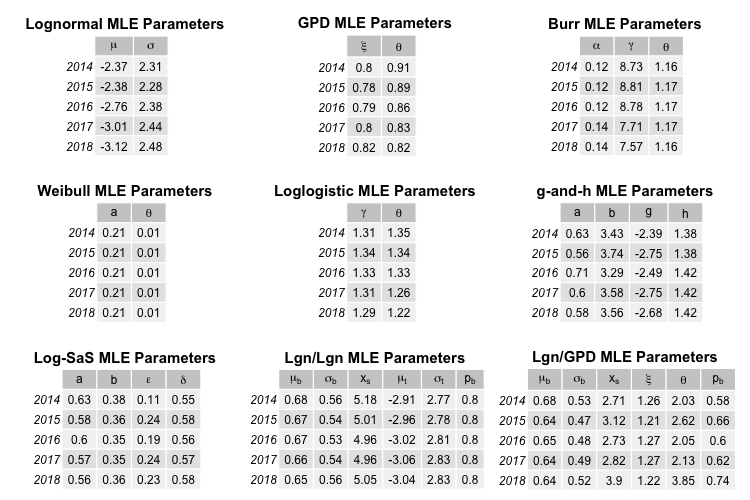
Figure A.1: The MLE from the simulated data ORC 3 for each candidate severity distribution for the years 2014 – 2018

Appendix B Loss Severity Distributions

When describing the right-tail behavior for the following loss severity distributions, the following notations are used: superexponential (SUPEX), subexponential (SUBEX), and regularly varying (RV).

Let $\Phi(\cdot)$ and $\phi(\cdot)$ represent the standard normal CDF and PDF, respectively. Let

$$A^{-1}_{g,h}\Bigg{(}\frac{x-a}{b}\Bigg{)}$$

be the inverse $g$-and-$h$ transformation function with location parameter $a$ and scale parameter $b$, and let

$$A_{\epsilon,\delta}^{-1}\Bigg{(}\frac{\log(x)-a}{b}\Bigg{)}$$

be the inverse log-SaS transformation function with location parameter $a$ and scale parameter $b$.

For the spliced distributions, $p_{b}$ is the proportion of the sample data that falls in the body of the sample, $x_{s}$ is the splicing point,

$$D_{1}({\Theta},\tau) =F_{body}(x_{s};{\Theta}_{b})-(1-p_{b})F_{body}(\tau;{\Theta}_{b});$$

$$D_{2}({\Theta},\tau) =\frac{1-p_{b}}{D_{1}({\Theta},\tau)}\ \frac{F_{body}(x_{s};{\Theta}_{b})-F_{body}(\tau;{\Theta}_{b})}{1-F_{tail}(x_{s};{\Theta}_{u})},$$

where $F_{body}$ is the lognormal distribution, and $F_{tail}$ is lognormal for the LGNLGN distribution and generalized Pareto for the LGNGPD distribution.

Candidate Severity Distribution Parameterizations

Distribution	$F(x;\Theta)$	Support	Right Tail
Lognormal	$\Phi\Big{[}\frac{\log(x)-\mu}{\sigma}\Big{]}$	$x\in\mathbb{R}$	SUBEX
Generalized	$1-\Big{(}1+\frac{\xi}{\theta}(x-u)\Big{)}^{-1/\xi}$	$x>u$	$\xi>0\implies$ RV
Pareto		$x>u$	$\xi=0\implies$ Exponential
		$u<x<u-\theta/\xi$	$\xi<0\implies$ Bounded above
Burr	$1-\Big{[}1+\big{(}\frac{x}{\theta}\big{)}^{\gamma}\Big{]}^{-\alpha}$	$x>0$	RV
Weibull	$1-\exp\Big{\{}-\big{[}\frac{x}{\theta}\big{]}^{a}\Big{\}}$	$x>0$	$a<1\implies$ SUBEX
			$a>1\implies$ SUPEX
Loglogistic	$\Big{[}1+\big{(}x/\theta\big{)}^{-\gamma}\Big{]}^{-1}$	$x>0$	RV
$g$-and-$h$	$\Phi\Big{[}A^{-1}_{g,h}\Big{(}\frac{x-a}{b}\Big{)}\Big{]}$	$x\in\mathbb{R}$	$h>0\implies$ RV
Log	$\Phi\Big{[}A_{\epsilon,\delta}^{-1}\Big{(}\frac{\log(x)-a}{b}\Big{)}\Big{]}$	$x>0$	$\delta\leq 0.5\implies$ RV
sinh-arcsinh			$0.5<\delta<1\implies$ SUBEX
			$\delta>1\implies$ SUPEX
Lognormal	$\dfrac{p_{b}}{D_{1}({\Theta},\tau)}\Phi\Big{[}\frac{\log(x)-\mu_{b}}{\sigma_{b}}\Big{]}$	$0<x\leq x_{s}$	SUBEX
Body
Spliced
	$\dfrac{p_{b}\Phi\Big{[}\frac{\log(x)-\mu_{b}}{\sigma_{b}}\Big{]}}{D_{1}({\Theta},\tau)}+D_{2}({\Theta},\tau)\Phi\Big{[}\frac{\log(x)-\mu_{t}}{\sigma_{t}}\Big{]}$	$x_{s}<x$
Lognormal
Tail	$\qquad-D_{2}({\Theta},\tau)\Phi\Big{[}\frac{\log(x_{s})-\mu_{t}}{\sigma_{t}}\Big{]}$
Lognormal	$\dfrac{p_{b}}{D_{1}({\Theta},\tau)}\Phi\Big{[}\frac{\log(x)-\mu_{b}}{\sigma_{b}}\Big{]}$	$0<x\leq x_{s}$	RV
Body
Spliced
Generalized	$\dfrac{p_{b}\Phi\Big{[}\frac{\log(x)-\mu_{b}}{\sigma_{b}}\Big{]}}{D_{1}({\Theta},\tau)}+D_{2}({\Theta},\tau)$	$x_{s}<x$
Pareto Tail	$\qquad-D_{2}({\Theta},\tau)\Big{\{}1+\frac{\xi}{\hat{\theta}}(x-x_{s})\Big{\}}^{-1/\xi}$

Table B.1: Table of candidate severity distributions, their parameterizations, support, and behavior of the right-tail of the density function, where regularly varying (RV) right tail if its density decreases to 0 at the rate $x^{-b}$ with $b>1$, subexponential (SUBEX) if its density decreases to 0 slower than $e^{-x}$, but faster than RV, or superexponential (SUPEX) if its density decreases to 0 faster than $e^{-x}$ (Foss et al.,, 2013).

References

- Akaike, (1974) Akaike, H. (1974). A new look at the statistical model identification. IEEE Transactions on Automatic Control, AC-19(6):716–723.
- Aldrich, (1997) Aldrich, J. (1997). R. A. Fisher and the making of maximum likelihood. Statistical Science, 12(3):162–176.
- Baud et al., (2003) Baud, N., Frachot, A., and Roncalli, T. (2003). How to avoid over-estimating capital charge for operational risk? Opertaional Risk - Risk’s Newsletter.
- BCBS, (2006) BCBS (2006). International convergence of capital measurement and capital standards. Technical report, Bank for International Settlements.
- BCBS, (2011) BCBS (2011). Operational risk - supervisory guidelines for the advanced measurement approaches. Technical report, Bank for International Settlements.
- BCBS, (2016) BCBS (2016). Standardised measurement approach for operational risk. Consultative document, Bank for International Settlements.
- Chavez-Demoulin et al., (2015) Chavez-Demoulin, V., Embrechts, P., and Hofert, M. (2015). An extreme value approach for modeling operational risk losses depending on covariates. The Journal of Risk and Insurance, 83(3):735–776.
- Chernobai et al., (2005) Chernobai, A., Menn, C., Truck, S., and Rachev, S. (2005). A note on the estimation of the frequency and severity distribution of operational losses. The Mathematical Scientist, 30(2):1–10.
- Chernobai et al., (2007) Chernobai, A., Rachev, S., and Fabozzi, F. (2007). Operational Risk: A Guide to Basel II Capital Requirements, Models, and Analysis. John Wiley & Sons, Inc.
- Degen et al., (2007) Degen, M., Embrechts, P., and Lambrigger, D. (2007). The quantitative modeling of operational risk: Between g-and-h and evt. Astin Bulletin, 37(2):265–291.
- Dutta and Perry, (2006) Dutta, K. and Perry, J. (2006). A tale of tails: An empirical analysis of loss distribution models for estimating operational risk capital. Working Papers 06-13, Federal Reserve Bank of Boston.
- Economist, (2016) Economist (2016). The final bill - financial crime. The Economist, 11.
- Embrechts and Hofert, (2011) Embrechts, P. and Hofert, M. (2011). Practices and issues in operational risk modeling under basel ii. Lithuanian Mathematical Journal, 51(2):180–193.
- Foss et al., (2013) Foss, S., Korshunov, D., and Zachary, S. (2013). An Introduction to Heavy-Tailed and Subexponential Distributions. Springer Science + Business Media New York, 2nd edition.
- Gneiting, (2011) Gneiting, T. (2011). Making and evaluating point forecasts. Journal of the American Statistical Association, 106(494):746–762.
- Hayahsi, l (20) Hayahsi, Y. (2018, April 20). Wells fargo to pay $1 billion to settle risk management claims. Wall Street Journal.
- Hoaglin, (1985) Hoaglin, D. (1985). Summarizing shape numerically: The g-and-h distributions. In Hoaglin, D., Mosteller, F., and Tukey, J., editors, Exploring Data Tables, Trends, and Shapes, chapter 11, pages 461–513. John Wiley & Sons, Inc.
- Jones and Pewsey, (2009) Jones, M. and Pewsey, A. (2009). Sinh-arcsinh distributions. Biometrika, 96(4):761–780.
- Luo et al., (2007) Luo, X., Shevchenko, P., and Donnelly, J. (2007). Addressing the impact of data truncation and parameter uncertainty on operational risk estimates. The Journal of Operational Risk, 2(4):3–26.
- Panjer, (2006) Panjer, H. (2006). Operational Risk: Modeling Analytics. John Wiley & Sons, Inc.
- Perline, (2005) Perline, R. (2005). Strong, weak and false inverse power laws. Statistical Science, 20(1):68–88.
- Peters and Shevchenko, (2015) Peters, G. and Shevchenko, P. (2015). Advances in Heavy Tailed Risk Modeling: A Handbook of Operational Risk. John Wiley & Sons, Inc.
- Schwarz, (1978) Schwarz, G. (1978). Estimating the dimension of a model. The Annals of Statistics, 6(2):461–464.
- Sinclair et al., (1990) Sinclair, C., Spurr, B., and Ahmad, M. (1990). Modified anderson-darling test. Communications in Statistics - Theory and Methods, 19(10):3677–3686.
- Strasburg, h (29) Strasburg, J. (2018, March 29). Barclays to pay $2 billion to resolve mortgage-securities claims. Wall Street Journal.