Enhancing Video Analytics Accuracy via Real-time Automated Camera Parameter Tuning

Abstract.

In Video Analytics Pipelines (VAP), Analytics Units (AUs) such as object detection and face recognition running on remote servers critically rely on surveillance cameras to capture high-quality video streams in order to achieve high accuracy. Modern IP cameras come with a large number of camera parameters that directly affect the quality of the video stream capture. While a few of such parameters, e.g., exposure, focus, white balance are automatically adjusted by the camera internally, the remaining ones are not. We denote such camera parameters as non-automated (NAUTO) parameters. In this paper, we first show that environmental condition changes can have significant adverse effect on the accuracy of insights from the AUs, but such adverse impact can potentially be mitigated by dynamically adjusting NAUTO camera parameters in response to changes in environmental conditions. We then present CamTuner, to our knowledge, the first framework that dynamically adapts NAUTO camera parameters to optimize the accuracy of AUs in a VAP in response to adverse changes in environmental conditions. CamTuner is based on SARSA reinforcement learning and it incorporates two novel components: a light-weight analytics quality estimator and a virtual camera that drastically speed up offline RL training. Our controlled experiments and real-world VAP deployment show that compared to a VAP using the default camera setting, CamTuner enhances VAP accuracy by detecting 15.9% additional persons and 2.6%–4.2% additional cars (without any false positives) in a large enterprise parking lot and 9.7% additional cars in a 5G smart traffic intersection scenario, which enables a new usecase of accurate and reliable automatic vehicle collision prediction (AVCP). CamTuner opens doors for new ways to significantly enhance video analytics accuracy beyond incremental improvements from refining deep-learning models.

1. Introduction

Significant progress in machine learning and computer vision techniques for analyzing video streams (imagenet, ), along with the explosive growth in Internet of Things (IoT), edge computing, and high-bandwidth access networks such as 5G (QUALCOMM-5G, ; CNET-5G, ), have led to the wide adoption of video analytics systems. Such systems deploy cameras throughout the world to support diverse applications in entertainment, health-care, retail, automotive, transportation, home automation, safety, and security market segments. The global video analytics market is estimated to grow from $5 billion in 2020 to $21 billion by 2027, at a CAGR of 22.70% (allied-market-research, ).

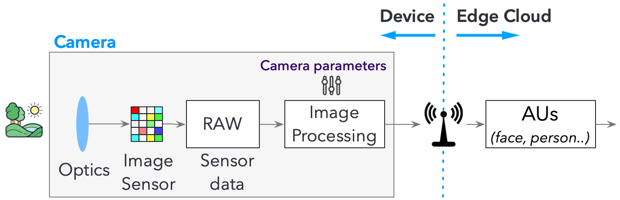
Figure 1. Video analytics pipeline.

A typical video analytics system consists of a video analytics pipeline (VAP) that starts with one or more surveillance cameras capturing live feed of the target environment. These live feeds are sent over a 5G network to servers at the edge of the 5G network where one or more analytics units (AUs) such as object detection, face detection, and face recognition use deep learning models to mine valuable information in the live video streams, as shown in Figure 1. These AUs critically rely on the cameras to capture high-quality real-time video streams in order to achieve high accuracy.

Modern IP cameras come with and expose a large number of camera parameters that direcly affect the quality of the video stream capture. While a few of such parameters, e.g., exposure, focus, white balance are automatically adjusted by the camera internally, the remaining camera parameters are not. We denote such camera parameters as non-automated (NAUTO) parameters.

In this paper, we first show that as the environmental conditions around the cameras change, the quality of video frames captured by the cameras also changes, and this can adversely affect the accuracy of insights derived by the analytics units. In our experiments, we kept all automatic parameter setting features turned on and thus our experiments show that those automatic settings are not enough to adapt to different environments for better analytics accuracy

Next, we experimentally show that by (manually) dynamically adjusting a prominent set of NAUTO camera parameters, in particular, four image appearance parameters including brightness, contrast, color-saturation (also known as colorfulness), and sharpness, which are available in both PTZ and non-PTZ cameras, it is possible to mitigate the potential loss in accuracy due to adverse environmental changes. We chose these NAUTO parameters in our study because they not only directly affect image qualities and hence AU accuracy but also are challenging to tune due to their large ranges of values.

Since streaming video analytics systems operate around the clock (24 hours a day, seven days a week), it is not practical for humans to manually adjust tens of configurable camera parameters in real-time in response to every environmental change. Therefore, we propose CamTuner, a system that detects and dynamically adapts to the changes in environmental conditions by automatically adjusting camera parameters in real-time to improve AU accuracy. CamTuner uses online reinforcement learning (RL) (introduction-to-rl, ) to continuously learn good camera settings and update the camera parameters to enhance the accuracy of the AUs in the VAP. In particular, CamTuner uses SARSA (q-lambda, ), which is faster to train and achieves slightly better accuracy in our video stream processing context than other popular RL approaches like Q-learning.

Although RL is a fairly standard technique, applying it to tuning camera parameters in a real-time video analytics system poses two unique challenges.

First, implementing online RL requires knowing the reward/penalty for every action taken during exploration and exploitation. Since no ground truth for an AU task like face detection is available during the online operation of a VAP, calculating the reward/penalty due to an action taken by an RL agent is a key challenge. To address this challenge, we propose an AU-specific analytics quality estimator that can accurately estimate the accuracy of the AU. Our estimator is light-weight, and it can run on a low-end PC or a simple IoT device to process video streams in real-time.

Second, bespoke online RL learning at each camera deployment setup requires initial RL training, which can potentially take a long time for two reasons: (1) capturing the environmental condition changes such as the time-of-the-day effect can take a long time, and (2) taking an action on the real camera (i.e., changing the camera parameter setting) by using the APIs provided by the camera vendor incurs a significant delay of about 200 ms. This limits the speed of state transitions during RL exploration, and hence the training speed of RL, to about 5 changes (actions) per second. To address these two sources of RL training inefficiencies, we propose a novel concept called virtual camera. A virtual camera mimics (in software) the effect of changing parameters of a physical camera to capture a scene. There are two key benefits of doing this: (1) we can complete an action of “camera setting change” almost instantaneously; and (2) we can digitally augment a single frame captured by the real camera to derive many new synthetically transformed frames, as if we had physically captured many different frames of the same scene by using a real camera at different environmental conditions (i.e., time-of-day, lighting conditions, seasonal changes etc.). These two benefits allow the RL agent to explore actions at a much faster rate than possible in using a real camera. This drastically reduces the RL training time required to develop a good, initial RL model, which can then be further refined in a short period (adaptation phase) after camera deployment.

Our paper makes the following contributions:

• We show that environmental condition changes can have a significant negative impact on the accuracy of AUs in video analytics pipelines, but the negative impact can be mitigated by dynamically adjusting a set of NAUTO camera parameters.

• We develop, to our knowledge, the first system that automatically and adaptively learns and tunes the set of NAUTO camera parameters in response to unpredictable environmental condition changes to improve the accuracy of insights from video analytics pipelines.

• We present two novel techniques that make the RL-based camera-parameter-tuning design feasible: a light-weight AU-specific analytics quality estimator that enables online RL without requiring ground truth, and a virtual camera that enables fast initial RL model training.

• We show that CamTuner improves AU accuracy in controlled experiments and in real VAP deployment. In particular, in a real world deployment where two cameras deployed side-by-side (one camera is managed by CamTuner, while the other is not) are monitoring a large enterprise parking lot, and the live video streams are carried over a 5G network, the camera managed by CamTuner detected 15.9% (146) additional persons (in a 5-minute span) during evening hours, without any false positives. The camera managed by CamTuner detected 2.6%–4.2% (861–881) additional cars (in a 5-minute span) during morning and evening hours, again without any false positives.

• Furthermore, by recording a real-world car accident scenario at a traffic intersection (at one of our customer locations) and by using VC to emulate frame captures at different times of the day, the VAP with CamTuner reliably detected 9.7% (122) additional cars (across the frames in a 1.5-minute span), which dramatically improves the accuracy (and lead time) of collision prediction.

• We show that CamTuner incurs very low computation overhead and CamTuner can be easily incorporated into VAPs that are executing on low-end PC or IoT devices that are directly attached to the camera.

2. Background

Figure 1 also shows the image signal processing (ISP) pipeline within a camera. Photons from the external world reach the image sensor through an optical lens. The image sensor uses a Bayer filter (bayer1976color, ) to create raw-image data, which is further enhanced by a variety of image processing techniques such as demosaicing, denoising, white balance, color-correction, sharpening and image compression (JPEG/PNG or video compression using H.264 (x264, ), VP9 (vp9, ), MJPEG, etc.) in the image-signal processing (ISP) stage (ramanath2005color, ) before the camera outputs an image or a video frame.

The camera capture forms the initial stage of the VAP, which may include a wide variety of analytics tasks such as face detection, face recognition, human pose estimation, license plate recognition etc. (see Figure 1).

Table 1. Parameters exposed by popular cameras. Parameters with “*” are auto-adjusted by the camera internally.

Camera Setting Parameters
Image	Brightness
Appearance	sharpness
	contrast
	color level
Exposure	Exposure Control∗
Settings	Max Exposure Time
	Exposure Zones∗
	Max gain
	IR cut filter∗
Image	Defog Effect
Correction	Noise Reduction
	Stabilizer
	Auto Focus Enabled∗
White	Type∗
Balance	window∗

Video Stream Parameters
Image	Resolution
Appearance	Compression
	Rotate image
Encoder	GOP length
Settings	H.264 profile
Bitrate	Type of Use
Control	Target Bitrate
	Priority
Video Stream	Max FPS
MJPEG	Max frame size

In this paper, we study video analytics applications that are based on surveillance cameras. Such cameras are running 24X7 in contrast to DSLR, point-and-shoot or mobile cameras that capture videos on-demand. Popular IP video surveillance cameras are manufactured by vendors such as AXIS (axis, ), Cisco (ciscocamera, ), and Panasonic (panasonic, ). These surveillance camera manufacturers have exposed many camera parameters via REST APIs which can be set by applications to control the image generation process, which in turn affects the quality of the produced image or video. The exposed parameters include those for changing the amount of light that hits the sensor, the zoom level and field-of-view (FoV) at the image-sensor stage, and those for changing the color-saturation, brightness, contrast, sharpness, gamma, acutance, etc. in the ISP stage. Table 1 lists the parameters exposed by a few popular surveillance cameras in the market today. Remotely changing the camera setting via the exposed APIs, however, incurs a significant delay, e.g., about 200 ms on Axis Q1615, Axis Q3515, Axis Q6128-E and Axis Q3505 MK II network camera.

While a few of these camera parameters, e.g., exposure, focus, balance, are automatically adjusted by the camera internally, the remaining camera parameters are not adjusted automatically. We denote such camera parameters as non-automated (NAUTO) parameters.

In this paper, we focus our study on the four image appearance camera parameters, denoted as I-A parameters in the rest of the paper, which are widely available in both PTZ and non-PTZ cameras: brightness, contrast, color-saturation (also known as colorfulness), and sharpness. We chose the above four NAUTO camera parameters in our study in this paper for two reasons: (1) they directly affect the quality of the image which is essential to AUs which typically extract insights, e.g., face recognition, from individual frames; (2) These parameters are more challenging to tune due to the large range (for example, between 1 and 100 for each of the parameters on Axis Q1615, Axis Q3515, Axis Q6128-E, Axis Q3505 MK II network camera etc.) compared to other NAUTO camera parameters which have either a few fixed settings or just a binary ON/OFF switch.

3. Motivation

We motivate the need for dynamically adjusting NAUTO camera settings by experimentally showing the impact of environmental changes on AU accuracy despite all the auto-setting features are left on, and that tuning a set of NAUTO camera settings can improve AU accuracy under the same environmental conditions.

3.1. Impact of Environment Change on AU Accuracy

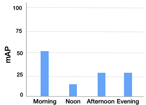
(a) Face detection

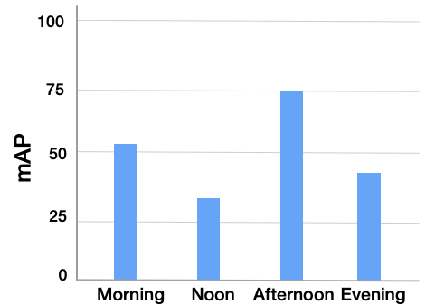
(b) Person detection

Figure 2. AU accuracy variation in a day under the default camera setting.

Environmental changes happen for at least three reasons. First, such changes can be induced due to the change of the Sun’s movement throughout a day, e.g., sunrise and sunset. Second, they can be triggered by changes in weather conditions, e.g., rain, fog, and snow. Third, even for the same weather condition at exactly the same time of the day, the videos captured by the cameras at different deployment sites (e.g., parking lot, factory, shopping mall, and airport) can have diverse content and ambient lighting conditions.

To illustrate the impact of environmental changes on image quality, and consequently on the accuracy of AUs, we experimentally measure the accuracy of two popular AUs (face detection and person detection) throughout a 24-hour (one-day) period. Since there are no publicly available video datasets that capture the environmental variations in a day or a week by using the same camera (at the same location), we use several proprietary videos provided by our customers that were captured with the default camera setting – in this paper, the default camera setting refers to when all auto-setting features are turned on and NAUTO parameters are set to the default values provided by the manufacturers. These videos were captured outside airports and baseball stadiums by stationary surveillance cameras, and we have labeled ground-truth information for several analytics tasks including face detection and person detection.

We use RetinaNet (deng2019retinaface, ) for face detection and EfficientDet-v8 (tan2020efficientdet, ) for person detection. We compute the mean Average Precision (mAP) by using pycocotools (pycoco, ). Figure 2(a) shows that the average mAP values for the face detection AU during four different time periods of the day (morning 8AM - 10AM, noon 12PM - 2PM, afternoon 3PM - 5PM, and evening 6PM - 8PM), and with the default camera setting, can vary by up to 40% as the day progresses (blue bars). Similarly, Figure 2(b) shows that the average mAP values for the person detection AU (with the default camera parameter setting) can vary by up to 38% during the four time periods. These results show that changes in environmental conditions can adversely affect the quality of the frames retrieved from the camera, and consequently adversely impact the accuracy of the insights that are derived from the video data.

3.2. Impact of Image Appearance Camera Settings on AU Accuracy

We experimentally show that adjusting the four image appearance (I-A) (NAUTO) camera settings, i.e., brightness, contrast, color-saturation (also known as colorfulness), and sharpness, can help to mitigate the adverse impact of environmental changes on AU accuracy.

Analyzing the impact of camera settings on video analytics in general faces a significant challenge: it requires applying different camera parameter settings to the same input scene and measuring the resulting accuracy of insights from an AU. The straightforward approach is to use multiple cameras with different camera parameter settings to capture the same input scene. However, this approach is impractical as there are thousands of different combinations of even just the four camera parameters we consider. To overcome the challenge, we proceed with the following workaround which uses a single real camera.

We use a real camera, Axis Q3505 MK II Network camera, to capture (at 10 FPS) the same real-world scene repeatedly under varying camera settings, and compare the accuracy of object detection AU for ”default” and several ”modified” settings – in this paper, a ”modified” setting refers to modifying the four I-A camera settings while keeping all other camera parameter values the same as the default setting. In our scene, two people walk from the camera towards two parked cars, and each of them then starts driving a separate car in a loop within the parking lot, parks the car in the same parking spot, and walks back towards the camera. The entire sequence of steps takes around 2 minutes and we repeat these exact steps over and over again for 26 different camera settings (including the ”default” setting). These experiments are conducted immediately one after another in quick succession to minimize the effect of environmental change.

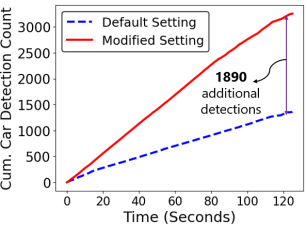
(a) Car Detection

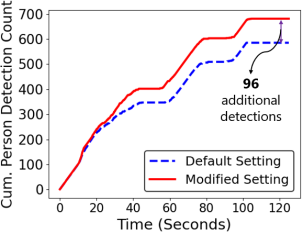
(b) Person Detection

Figure 3. Impact of camera settings on object detection.

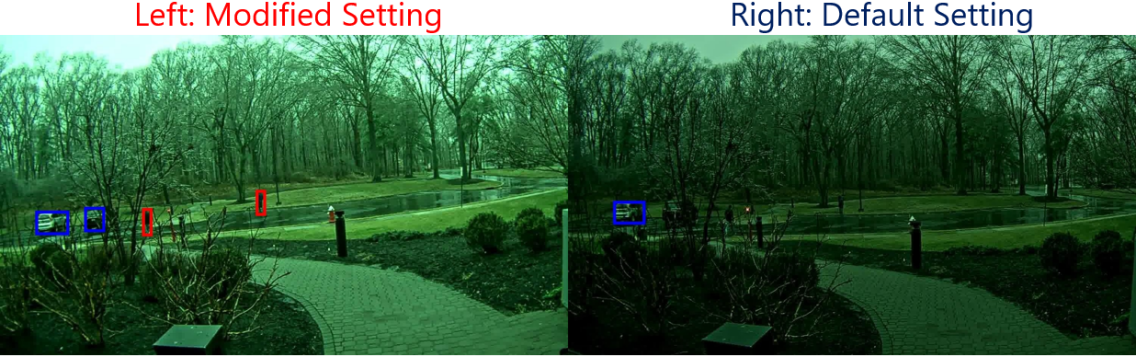
Figure 4. Same scene with different camera settings.

We consider object detection AU in this experiment, which detects cars and persons in the scene. Specifically, we use Efficientdet (tan2020efficientdet, ) object detector. An illustration of the scene is shown in Figure 4 with two side-by-side frames, where the right one is with the ”default” camera setting and the left one is with a ”modified” camera setting. Here, the AU can accurately detect two persons and two cars on the frame with the modified camera setting while from the camera capture under the default setting, the AU can only detect one car. We observe that the accuracy of the AU varies across different camera settings and Figure 3 shows the cumulative number of true-positive car and person detection counts  for ”Default Setting” and for ”Modified Setting”, which shows the highest accuracy among the 25 different camera settings. We see that ”Modified Setting” correctly detected 1890 additional cars and 96 additional persons across 1300 frames compared to “Default Setting”.

Table 2. Best settings for different environment.

Environment	Best Camera Setting
(Time-of-day)	[brightness, contrast, color, sharpness]
Dawn	[80, 75, 50, 75]
Morning	[30, 30, 50, 50]
Evening	[90, 90, 50, 50]

To understand if the modified camera setting that provides the highest AU accuracy remains the same as the environment undergoes changes, we repeat the above experiment for three different times of the day, i.e., dawn, morning and evening, which have varying sunlight, while enacting the same scene for camera capture.  Table 2 shows that the I-A camera setting that provides the highest AU accuracy is not the same as the manufacturer-provided default setting and it varies for different times of the day, i.e., different environmental conditions.

3.3. Optimal camera setting is AU-specific

Along with the environment, to observe the impact of camera parameters on various AUs, we printed 12 different person cutouts obtained from COCO dataset (lin2014microsoft, ) and placed them in front of an Axis network camera. we use Efficientdet (tan2020efficientdet, ) as person-detection AU and RetinaNet (deng2019retinaface, ) as face-detection AU and observe the impact on each of these AUs individually under DAY and NIGHT condition simulated inside our lab using two light sources. One of them is always kept ON, while the other light source is manually turned ON or OFF to simulate DAY and NIGHT environmental conditions, respectively. For each of these conditions, we vary the four image appearance camera parameters, i.e., brightness, contrast, sharpness and color-saturation ranging from 0 to 100 at a step of 10.  Figure 5 shows the images captured under the default camera setting for DAY and NIGHT condition. To find the “Best” settings for a specific AU, we change the four camera parameters to find the setting that gives the highest mAP. Specifically, we vary each parameter from 0 to 100 in steps of 10 and capture the frame for each camera setting. This gives us $\approx$14.6K (11⁴) frames for each condition. Changing the camera setting through the VAPIX API takes about 200ms, and in total it took about 7 hours to capture and process the frames for each condition.

Table 3 shows that the best I-A camera parameter setting for different AUs are unique. Furthermore, these Best camera settings not only vary across different AUs but change due to environmental condition changes (i.e., from DAY to NIGHT), also shown in  Table 3. This motivates the need for capturing AU specific perception in tuning the camera parameters.

(a) DAY

(b) NIGHT

Figure 5. Camera captures under different environment and visual impact.

Table 3. Best settings across different AUs for various env.

AU-best	Best camera setting
	[brightness, contrast, color, sharpness]
	DAY	NIGHT
Person Detection-best	[80,90,70,100]	[40,90,60,100]
Face Detection-best	[80,90,60,80]	[60,40,90,90]

4. Challenges and Approaches

Designing CamTuner to automatically tune camera parameter settings to enhance video analytics accuracy faces several challenges. In this section, we discuss these challenges and our approaches to address each one of them.

Challenge 1: Identifying the best camera setting for a particular scene. Cameras deployed across different locations observe different scenes. Moreover, the scene observed by a particular camera at any one location keeps changing based on the environmental conditions, lighting conditions, movement of objects in the field of view, etc. In such a dynamic environment, how can we identify the best camera setting that will give the highest AU accuracy for a particular scene? The straightforward approach of collecting data for all possible scenes that can ever be observed by the camera and training a model that gives the best camera settings for a given scene is infeasible.

Approach. To address this challenge, we propose to use an online learning method. Particularly, we use Reinforcement Learning (RL)  (introduction-to-rl, ), in which the agent learns the best camera settings on the go. Out of several recent RL algorithms, we choose the SARSA (q-lambda, ) RL algorithm for identifying the best camera settings (more details provided in §5.1).

Challenge 2: No Ground truth in real-time. Implementing online RL requires knowing the reward/penalty for every action taken during exploration and exploitation, i.e., what effect a particular camera parameter setting will have on the accuracy change of the AU. Since no ground truth of the AU task, e.g., face detection, is available during normal operation of the real-time video analytics system, detecting a change in accuracy of the AU during runtime is challenging.

Approach. We propose to estimate the accuracy of the AU. Each AU, depending on its function has a preferred method of measuring accuracy, e.g., for face detection AU, a combination of mAP and true-positive IoU is used, whereas for face recognition AU, the true-positive match score is used. Accordingly, we propose to have a separate estimator for each AU. We design such AU-specific analytics quality estimators to be light-weight so that they can be used by the RL agent in real-time (more details provided in §5.2).

Challenge 3: Extremely slow initial RL training. Online learning at each camera deployment setup requires initial RL training, which can potentially take a very long time for two key reasons: (1) Capturing the environmental condition changes such as the time-of-the-day effect requires waiting for the Sun’s movement through the entire day until night, and capturing weather changes requires waiting for weather changes to actually happen. (2) Taking an action on the real camera, i.e., changing the camera parameter setting, incurs a significant delay of about 200 ms. This delay fundamentally limits the speed of state transition and hence the learning speed of RL to only 5 actions per second.

Approach. In order to speed up the initial RL training, we propose a novel concept called Virtual Camera (VC). A VC mimics the effect of environmental conditions and camera setting changes on the frame capture of a real camera. This has two immediate benefits. First, it can effectively complete an action of “camera setting change” almost instantaneously. Second, it can augment a single frame captured by the real camera with many new transformed frames as if they were captured by the real camera under different conditions. Together, these two benefits allow the RL system to explore an order of magnitude more states and actions per unit time (more details provided in §5.3).

5. ${\sc CamTuner}$ Design

Figure 6 shows the system-level architecture for CamTuner, which automatically and dynamically tunes the camera parameters to enhance the accuracy of AUs in the VAP. CamTuner augments a standard VAP shown in Figure 1 with two key components: a Reinforcement Learning (RL) engine, and an AU-specific analytics quality estimator. In addition, it employs a third component, a Virtual Camera (VC), for fast initial RL training.

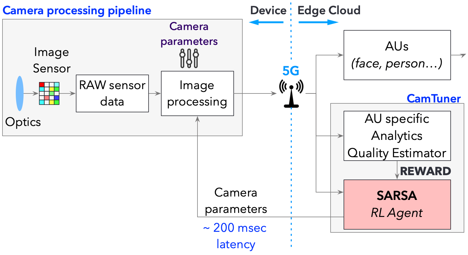
Figure 6. ${\sc CamTuner}$ system design.

5.1. Reinforcement Learning (RL) Engine

The RL engine is the heart of CamTuner system, as it is the one that automatically chooses the best camera settings for a particular scene. Q-learning (q-learning, ) and SARSA (q-lambda, ) are two popular RL algorithms that are quite effective in learning the best action to take in order to maximize the reward. We compared these two algorithms and found that training with SARSA achieves slightly faster convergence and also slightly better accuracy than with Q-learning. Therefore, we use SARSA RL algorithm in CamTuner.

SARSA is similar to other RL algorithms. An agent interacts with the environment (state) it is in, by taking different actions. As the agent takes actions, it moves into a new state or environment. For each action, there is an associated reward or penalty, depending on whether the new state is desirable or not. Over a period of time, as the agent continues taking actions and receiving rewards and penalties, it learns to maximize the rewards by taking the right actions, which ultimately lead the agent towards desirable states.

SARSA does not require any labeled data or pre-trained model, but it does require a clear definition of the state, action and reward for the RL agent. This combination of state, action and reward is unique for each application and needs to be carefully chosen, so that the agent learns exactly what is desired. In our setup, we define them as follows:

State: A state is a tuple of two vectors, $s_{t}=<P_{t},M_{t}>$, where $P_{t}$ consists of the current brightness, contrast, sharpness, and color-saturation parameter values on the camera, and $M_{t}$ consists of the measured values of brightness, contrast, color-saturation, and sharpness of the captured frame at time $t$, measured as in (bezryadin2007brightness, ; peli1990contrast, ; hasler2003colormeasuring, ; de2013sharpness, ).

Action: The set of actions that the agent can take are (a) increase or decrease one of the brightness, contrast, sharpness or color-saturation parameter value, or (b) not change any parameter values.

Reward: We use an AU-specific analytics quality estimator as the immediate reward function (r) for the SARSA algorithm. Along with considering immediate reward, the agent also factors in future reward that may accrue as a result of the current actions. Based on this, a value, termed as Q-value (also denoted as $Q(s_{t},a_{t})$) is calculated for taking an action $a_{t}$ when in state $s_{t}$ using Equation 1.

(1) $$\vspace{-0.05in}Q(s_{t},a_{t})\leftarrow Q(s_{t},a_{t})+\alpha\left[r+\gamma\cdot Q(s_{t+1},a_{t+1})-Q(s_{t},a_{t})\right]$$

Here, $\alpha$ is learning rate (a constant between 0 and 1) used to control how much importance is to be given to new information obtained by the agent. A value of 1 will give high importance to the new information while a value of 0 will stop the learning phase for the agent.

Similar to $\alpha$, $\gamma$ (also known as the discount factor) is another constant used to control the importance given by the agent to any long term rewards. A value of 1 will give very high importance to long term rewards while a value of 0 will make the agent ignore any long term rewards and focus only on the immediate rewards. If the environmental conditions change very frequently, a lower value, e.g., 0.1, can be assigned to $\gamma$ to prioritize immediate rewards, while if the conditions do not change frequently, a higher value, e.g., 0.9, can be assigned to prioritize long term rewards.

Exploration vs. Exploitation. We define a constant called $\epsilon$ (between 0 and 1) to control the balance between exploration vs. exploitation in taking actions. At each step, the agent generates a random number between 0 and 1; if the random number is greater than the set value of $\epsilon$, then a random action (exploration) is chosen.

5.2. AU-specific Analytics Quality Estimator

In online operations, the RL engine needs to know whether its actions are changing the AU accuracy in the positive or negative direction. In the absence of ground truth, the analytics quality estimator acts as a guide and generates the reward/penalty for the RL agent.

Challenges. There are three key challenges in designing an online analytics quality estimator. (1) During runtime, AU quality estimation has to be done quickly, which implies a model that is small in size. (2) A small model size implies using a shallow neural network. For such a network, what representative features should the estimator extract that will have the most impact on the accuracy of AU output? (3) Since different types of AUs (e.g., face detector, person detector) perceive the same representative features differently, the estimator needs to be AU-specific.

Insights. We make the following observations about estimating the quality of AUs. (1) Though estimating the precise accuracy of AU on a frame requires a deep neural network, estimating the coarse-grained accuracy, e.g., in increments of 1%, may only require a shallow neural network. (2) Most of the “off-the-shelf” AUs use convolution and pooling layers to extract representative local features (low-level-features, ). In particular, the first few layers in the AUs extract low-level features such as edges, shapes, or stretched patterns that affect the accuracy of the AU results. We can reuse the first few layers of these AUs in our estimator to capture the low-level features. (3) To capture different AU perceptions from the same representative features extracted in the early layers, we need to design and train the last few layers of each quality estimator to be AU-specific. During training, we need to use AU-specific quality labels.

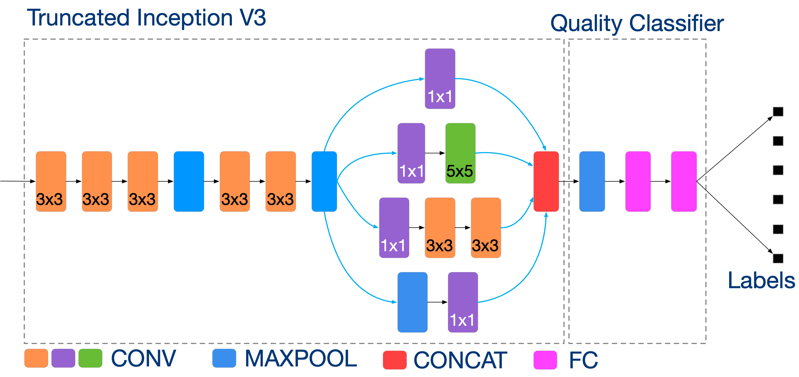
Figure 7. AU-specific analytics quality estimator design.

Design. Motivated by the above insights, we design our light-weight AU-specific analytical quality estimator to consist of two components: (1) feature extractor and (2) quality classifier, as shown in  Figure 7. We use supervised learning to train the AU-specific quality estimator.

Feature Extractor. Different AUs and environmental conditions can manipulate local features of an input frame at different granularities (GUPTA2021100057, ). For example, blur (i.e., motion or defocus blur) affects fine textures while light exposure affects coarse textures. While face detector and face recognition AUs focus on finer face details, person detector is coarse-grained and it only detects the bounding box of a person. Similarly, in convolution layers, larger filter sizes focus on global features while stacked convolution layers extract fine-grained features. To accommodate such diverse notions of granularities, we use the Inception module from the Inception-v3 network (inception-v3, ), which has convolution layers with diverse filter sizes.

Quality classifier. The goal of the quality classifier is to take the features extracted by the feature extractor and estimate the coarse-grained accuracy of the AU on an input frame, e.g., in increments of 1%. As such, we divide the AU-specific accuracy measure into multiple coarse-grained labels, e.g., from 0% to 99%, and use fully-connected layers whose output nodes generate AU-specific classification labels.

Detailed design and training of two concrete AU-specific analytics quality estimators are described as follows.

(1) Face recognition AU: The quality classifier of face recognition consists of 2 fully-connected layer and has 101 output classes. One of the classes signifies no match, while the remaining 100 classes correspond to match scores between 0 to 100% in units of 1%.

To generate the labeled data, we used 300 randomly-sampled celebrities from the celebA dataset (liu2015faceattributes, ). We choose two images per person. We use one of them as a reference image and add it to the gallery. We use the other image to generate multiple variants by applying digital transformations on the image. These variants ($\sim$4 million) form the query images. For each query image, we obtain the match score (a value between 0 and 100%) using the Face recognition AU, Neoface-v3. The query images along with their match score form the labeled samples, which are used to train the quality estimator.

(2) Face and object detection AU. The quality classifier of face and object (i.e., car and person) detection AU consists of 2 fully-connected layers, and has 201 output classes to predict the quality estimate of the face and object detection AU for a given frame. One of the classes signifies AU cannot detect anything accurately, and the remaining 200 classes correspond to the cumulative mAP score between 0 to 100 and IoU score between 0 to 1, i.e., $mAP+IOU_{True-Positive}*100$. To generate the labeled data to train face-detection AU specific quality estimator, we used the Olympics (niebles2010modeling, ) and HMDB (Kuehne11, ) datasets, and created $\sim$7.5 million variants of the video frames by applying digital transformations. Then, for each frame, we use the face detection AU (i.e., RetinaNet (deng2019retinaface, )) to determine the analytical quality estimate. Similarly, we use the object detection AU (i.e., EfficientDet (tan2020efficientdet, )) on labeled images from COCO dataset (lin2014microsoft, ) that contain car and person object classes and their augmented variants. The video frames/images and their quality estimates form the labeled samples, which are used to train the estimator model.

For both the classifier training, we use a cross-entropy loss function to train AU-specific analytics quality estimators, initial learning rate is $10^{-5}$, and we use Adam Optimizer (kingma2014adam, )

5.3. Virtual Camera

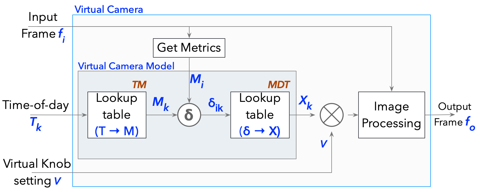
Figure 8. VC block diagram.

Definition. A VC (shown in Figure 8) takes an input frame $f_{i}$, captured by a real camera, the target time-of-the-day $T_{k}$, and VC parameter settings $V$, as input, and outputs a frame $f_{o}$ as if it was captured by the physical camera at time $T_{k}$. To generate a frame at time $T_{k}$, VC uses a composition function $Compose(X_{k},V)$, which composes output frame $f_{o}$ using $X_{k}$, which is the transformation that augments the environmental effects corresponding to the target time $T_{k}$ on input frame $f_{i}$, and $V$, which is the VC parameter settings. The composition function is defined as $X_{k}*10^{V-0.5}$, which considers $X_{k}$ and $V$ simultaneously, similar to a real camera. Using this composition function, $X_{k}$ is scaled up if the value of $V$ is greater than 0.5 and scaled down if the value is less than 0.5; no scaling of $X_{k}$ happens for $V$ equal to 0.5.

To understand how VC works, we first introduce an important definition. Each frame $f_{i}$, from a real physical camera, possesses distinct values of brightness, contrast, colorfulness and sharpness metrics, denoted as a metric (or feature) tuple $M_{i}=<\alpha_{M}$, $\beta_{M}$, $\gamma_{M}$, $\zeta_{M}>$. The unique metric tuple encapsulates the environmental conditions and the default physical camera settings when the frame was captured.

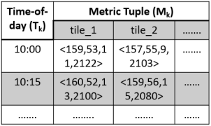
(a) TM table

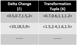
(b) MDT Table

Figure 9. Offline generated tables for VC.

Offline profiling phase: VC derives two tables for a given physical camera deployment during an offline profiling phase and then uses the two tables during online operation to generate the output frame $f_{o}$.

The first table (TM) maps a given time-of-the-day $T_{k}$ to the metric tuple $M_{k}$ which captures the distinct values of brightness, contrast, colorfulness and sharpness metrics of frames taken by the physical camera with the default settings at time $T_{k}$. We generate the table to cover the full 24-hour period with a granularity of 15 minutes, i.e., the table has one mapping for every 15 minutes, for a total of 96 mappings. To construct the table, we use a full 24-hour long video and break it into 15-minute video snippets. We extract all the frames from the video snippet for each 15-minute interval $T_{k}$. We divide each frame into 12 tiles, obtain the corresponding metric tuple for each tile, and compute the mean metric tuple for the corresponding tiles in all frames in the 15-minute interval as the metric tuple for that tile, and the list of tuples for all 12 tiles form the entry for time $T_{k}$ in the table, as shown in Figure 9(a).

The second table (MDT) maps the difference between two metric tuples $M_{i}$ and $M_{k}$, $\delta(M_{i},M_{k})$, to the corresponding transformation tuple $X_{k}$ that would effectively transform a frame captured by the physical camera with metric tuple $M_{i}$ to become a frame captured by the physical camera for the same scene with metric tuple $M_{k}$. We note since each camera parameter can take 11 values, from 0 to 100 with increments of 10, the difference between any two metric tuples can possibly be mapped to one of these 14K ($11^{4}$) settings. We construct the entries for the table backward as follows. (1) We select a random frame from each 15-minute interval to form a collection of 96 frames with varying environmental conditions, i.e., corresponding to different time-of-the-day. (2) For each possible transformation $X_{k}$, we transform the 96 frames into 96 virtual frames. We then obtain the delta metric tuples between each pair of original and transformed frames, calculate the median of the 96 delta metric tuples, $\delta_{k}$, and store the pair of $<\delta_{k},X_{k}>$ in the table. (3) We repeat the above process for all possible transformation settings (14K in total) to populate the table, as shown in Figure 9(b).

Finally, at runtime when the table is used by the VC, if the entry for a given delta metric tuple $\delta_{i}$ is empty, we return the entry whose delta metric tuple $\delta_{k}$ is closest to $\delta_{i}$ using L1-norm.

Online phase. VC transforms the input frame $f_{i}$ to output frame $f_{o}$ in five steps. (1) It measures the current metric tuple $M_{i}=<\alpha_{M}$, $\beta_{M}$, $\gamma_{M}$, $\zeta_{M}>_{curr}$ from input frame $f_{i}$; (2) It looks up Time-to-Metric (TM) table for the metric tuple $M_{k}=<\alpha_{M}$, $\beta_{M}$, $\gamma_{M}$, $\zeta_{M}>_{desired}$ that corresponds to the target time of the day ($T_{k}$); (3) It calculates the difference between $M_{i}$ and $M_{k}$, $\delta(M_{i},M_{k})$ or $\delta_{ik}$; (4) It looks up Metric-difference-to-Transformation (MDT) table to find the transformation $X_{k}=<\alpha_{X}$, $\beta_{X}$, $\gamma_{X}$, $\zeta_{X}>_{applied}$ that corresponds to $\delta_{ik}$; (5) It applies $X_{k}$ along with $V$ using the composition function $Compose(X_{k},V)$ to input frame $f_{i}$ and generates output frame $f_{o}$.

Since different parts of an input frame may exhibit varying local feature or metric values, to improve the effectiveness of virtual knob transformation, instead of applying the above steps directly to input frame $f_{i}$, we split it into 12 (3 $X$ 4) equal-sized tiles, apply Steps 1-3 to each of the 12 tiles, i.e., each of $M_{i}$, $M_{k}$, and $\delta_{ik}$ consists of 12 sub-tuples corresponding to the 12 tiles, respectively. The 12 sub-tuples in $\delta_{ik}$ are looked up in the MDT table to find 12 transformation tuples. Finally, to ensure smoothness, we calculate the mean of these 12 sub-tuples $X_{k}$, which is then applied to input frame $f_{i}$.

5.4. Integrating VC with the RL engine

During initial RL training, the RL agent performs fast exploration by leveraging VC as follows. It reads each frame $f_{i}$ from the input training video, and repeats the following exploration steps for all time-of-the-day values $T_{k}$. At each exploration step $j$, the agent which is at state $s=<P_{j},M_{j}>$ performs tasks: (1) based on current state (s), it takes a random action $a$ and apply that on $V_{j}$, which is VC equivalent of $P_{j}$ for a real camera, to get a new virtual knob setting for next exploration step ($j+1$), $V_{j+1}$; (2) it invokes the VC with frame $f_{i}$ for the target time-of-the-day $T_{k}$, and current VC parameters $V_{j+1}$ as input, and the VC outputs frame $f_{o}$. The measured tuple $M_{j+1}$ of brightness, contrast, colorfulness and sharpness metric values of output frame $f_{o}$ along with the virtual knob setting $V_{j+1}$, form the new state of the RL agent, $s_{new}=<V_{j+1},M_{j+1}>$; (3) it calculates the reward/penalty by feeding $f_{o}$ into the AU-specific quality estimator; and (4) it updates the Q-table entry $Q(s,a)$.

The above initially trained SARSA model with the VC is then deployed in the real camera for the normal operations of CamTuner. First, the $\epsilon$ value is set to low (0.1) and $\alpha$ is set to high (0.85) so that the SARSA RL agent will go through a short adaptation phase, e.g., for an hour, by performing primarily exploration. Afterward, the $\epsilon$ and $\alpha$ values are set to high (0.9) and low (0.15), respectively, so that SARSA performs primarily exploitation using the trained model.

6. Implementation

6.1. Hardware Setup

For the evaluation, we implemented a VAP using an Axis Q3505 MK II network surveillance camera. We run CamTuner on a low-end Intel NUC box while face detection and object detection AUs and initial pre-training with VC run on a high-end edge-server equipped with Xeon(R) W-2145 CPU and GeForce RTX 2080 GPU. The captured frames are sent for AU processing on the edge-server over a 5G network with an average frame uploading latency of 39.7 ms.

6.2. Software Implementation

We implemented the SARSA RL agent in Python, the light-weight AU-specific analytics quality estimators in pytorch framework which runs as a service using the ZeroMQ (zeromq, ) networking library, and the Virtual Camera in Python which is trained on the GPU edge server. We use PIL (pil, ) and OpenCV (cv2, ) for image processing during the offline profiling phase in VC design and also during offline training of the SARSA RL agent. We use Axis’ VAPIX API to change the camera parameters decided by the SARSA-RL agent as well as to capture input frames.

Similar to a real camera, our VC runs continuously during offline SARSA RL training and streams the output frames on a NATS (nats, ) queue at the same frames-per-second (FPS) with which the video was captured. Each frame is sent in BSON format which includes the frame number, frame data (i.e., array of bytes), and timestamp. Like a real camera, VC exposes REST APIs that are used to query and change its settings to allow augmenting various environmental effects.

7. Evaluation

We extensively evaluate the effectiveness of CamTuner by measuring its impact on AU accuracy improvement in a VAP via controlled experimental emulation and in a real deployment (§7.1 – §7.4). We also evaluate its system performance (§7.5) and the efficacy of its two key components, AU-specific analytics quality estimator and VC (§7.6).

7.1. End-to-end VAP Performance

We first evaluate the effectiveness of CamTuner by comparing AU accuracy of five different VAPs.

7.1.1. Experimental Setup

We compare three CamTuner variants against two baseline VAPs. All system variants, including CamTuner, only differ in how the four I-A camera parameters are tuned, while keeping all automatic parameter setting features turned on and the rest NAUTO parameters at the default values. (1) Baseline: In the Baseline VAP, the I-A camera parameters are not adapted to any environmental changes. (2) Strawman: The Strawman approach applies a time-of-the-day heuristic that tunes the four I-A camera parameters based on a human perception metric. In particular, we use the BRISQUE quality metric (brisque_mittal2012no, ) and exhaustively search for the best camera parameters for the first few frames in each hour and then apply the best camera setting found for the remaining frames in that hour. This exhaustive search of camera settings using initial frames takes a few minutes and our results show that performing this adaptation more often than once per hour does not give significant improvement. (3) CamTuner-$\beta$: This variant of CamTuner only uses a few rounds of online exploration (i.e., which takes about 1 hour, same as in online exploration performed by CamTuner), i.e., the SARSA RL agent does not rely on the VC for initial offline exploration. Instead, at the start of online exploration, the CamTuner-$\beta$ framework is initially seeded with an empty Q-table. (4) CamTuner-$\alpha$: This variant of CamTuner adjusts the I-A camera setting dynamically by using only the offline trained SARSA RL agent, i.e., the agent does not perform any exploration during online operation. (5) CamTuner: The complete CamTuner framework is seeded with offline trained SARSA RL agent, and then during online operation, the agent continues exploration initially and then moves towards exploitation, as described in §5.4. For CamTuner-$\beta$, CamTuner-$\alpha$ and CamTuner, the RL agent adaptively adjusts the four I-A camera parameters periodically; the time interval is configurable and we choose it to be 10s.

Experimental methodology. Comparing these 5 VAPs in a real-world deployment is difficult because (1) even with 5 co-located cameras, it is difficult to see the identical scene from the same angle; (2) furthermore, in a real-world deployment, the captured scenes do not have the ground-truth to measure the AU accuracy. To overcome the above challenge, we loop a pre-recorded (original) 5-minute video snippet (a customer video captured at an airport) labeled with ground-truth through VC – VC is used here not for RL training but for generating augmented input videos that emulate different environmental changes to be fed into the five VAPs. In particular, we gradually change the VC model parameters (i.e., digital transformations) to simulate the changes that happen during the day as the Sun changes its position and finally sets, and we ensure (through manual inspection) that same ground-truths are carried over in the VC generated videos from the original video. We then project these VC-generated videos on a monitor screen in front of a real camera, and run each of the five VAPs in turn. We note that the above controlled experimental setup is the closest approximation to a real-world deployment.

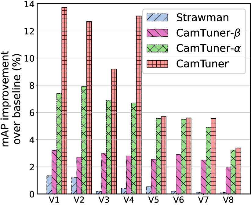
(a) Face detection AU

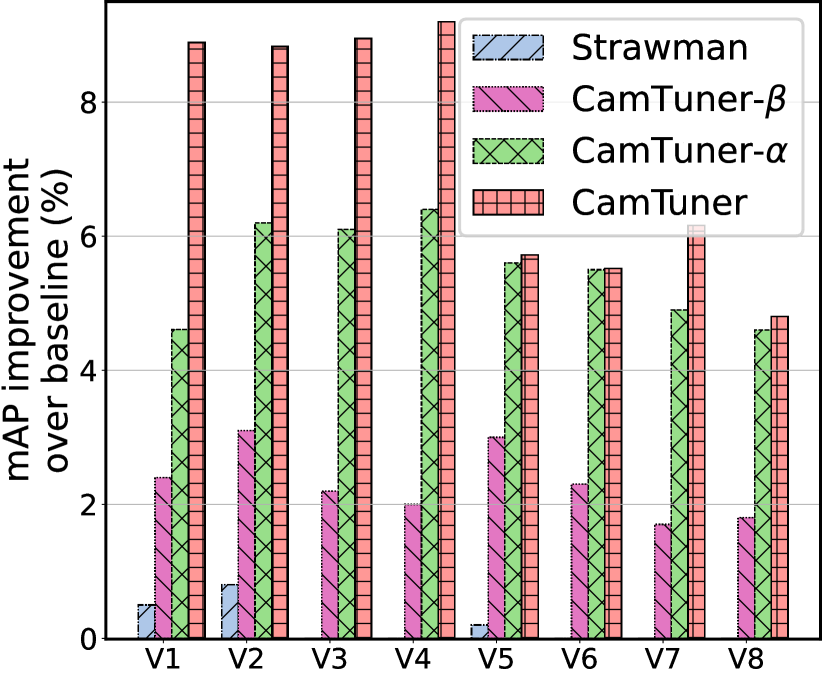
(b) Person detection AU

Figure 10. mAP improvements for different AUs.

7.1.2. End-to-end Accuracy

We evaluate the AU accuracy improvement of VAPs 2-5 over VAP 1 for eight 5-minute video segments randomly selected from the VC-generated videos consisting of 7500 frames each, and the video segments are separated by 1 hour apart. Using the labeled ground-truth, we evaluate the detection accuracy of the 5 VAPs for face-detection and person-detection AUs.

Figure 10 shows the bar-plot of mAP improvement of VAPs 2-5 over VAP 1 for the eight 5-min video segments corresponding to eight different hours of the day. We make the following observations. The strawman approach based on the time-of-the-day heuristic can provide only nominal improvement over Baseline, i.e., less than 1% on average across the videos for both face detection and person detection. Just a few hours of slow online exploration (i.e., with no VC-accelerated offline exploration) enables CamTuner-$\beta$ to improve face detection accuracy by 2.70% on average and person detection accuracy by 2.31% on average over Baseline. In contrast, fast offline exploration using virtual camera (with no online exploration) helps CamTuner-$\alpha$ to improve face detection accuracy by 6.01% on average and person detection accuracy by 5.49% on average over Baseline. Finally, dynamically tuning the real camera parameters with online learning in CamTuner improves the face detection AU accuracy by up to 13.8% and person detection AU accuracy by up to 9.2%, with an average improvement of 8.63% and 8.11% for face detection AU, and average improvement of 7.25% and 7.08% for person detection AU compared to Baseline and Strawman, respectively.

In summary, during offline phase VC helps the SARSA RL agent to quickly train through fast and equivalent environmental changes and camera parameter changes applied to the input scene. Then during online operation, a few rounds of exploration helps CamTuner to achieve better accuracy than directly using the initially trained SARSA model with VC (CamTuner-$\alpha$).

7.1.3. In-depth Analysis

Next, we show how CamTuner dynamically adjusts the camera parameter setting for one of the 5-minute video snippet (i.e., V3 in Figure 10) used in §7.1.2 for face-detection AU. Recall at every 10 seconds, based on the current environmental condition and content seen by the camera, CamTuner either chooses to “increment” or “decrement” one of the four parameters, i.e., increase or decrease by 10 within the parameter range of [0, 100], or keep the previous parameter setting.  Figure 11(a) shows how the camera parameters are adapted throughout the video length during the exploitation phase, and  Figure 11(b) shows how the corresponding mean intersection-over-union (mIoU) (i.e., IoU across all ground-truth bounding boxes in each frame) varies for the CamTuner-based VAP and the Baseline VAP.

We make the following observations. (1) Starting with the default camera parameter setting, i.e., [50, 50, 50, 50], CamTuner decrements the sharpness parameter after looking into the initial two frames, and then decrements contrast after 7 tuning intervals (at 70^th second). At the $13^{th}$ tuning interval, it increments a third parameter, brightness. Then again after two intervals (at 150^th second), it increments the sharpness parameter. In the subsequent interval, CamTuner decides to decrement color-saturation after looking into the most recently captured scene. Finally, CamTuner further decrements the sharpness parameter three more times where the first two are separated by 10s but the last parameter change (at 270^th second) happens after a 90s gap. Throughout the 5-minute video, CamTuner adjusts the camera setting 8 times. The camera setting adaption improves the mIoU per frame by 0.026 on average with the maximum mIoU improvement of 0.67 in comparison with using the default camera parameter setting. (2) CamTuner improves the mIoU for 24.8% of the video frames (by a maximum of 0.67) and only minimally reduces the mIoU for 1.6% of the frames (by a maximum of 0.005). An mIoU value of zero implies that no face in the input scene is detected by the face-detection AU. (3)  Figure 11(b) also shows that while faces are not detected under the default setting for 2.4% of the frames, the face-detection AU can detect faces in those frames once CamTuner adapts the camera parameters.

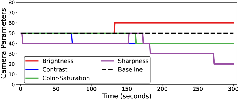
(a) Camera setting adaptation

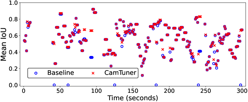
(b) mIoU variation

Figure 11. ${\sc CamTuner}$ in operation.

7.2. How quickly does CamTuner react to suboptimal settings

Here, we evaluate how quickly CamTuner can react if the camera is set to a suboptimal setting that leads to degraded analytical outcome. We place two side-by-side cameras in front of a scene consisting of 3D objects as shown in Figure 12. In this scene, 3D slot cars are continuously moving over the track and 3D human models are kept stationary. Both cameras start with a same suboptimal setting (we use two suboptimal settings denoted as SS1 and SS2) and stream at 10 FPS for 2-minute period, during which the I-A parameters of Camera 1 are kept to the same initial suboptimal values, while the I-A parameters of Camera 2 are tuned by CamTuner every 2s. On every frame streamed from camera, we use Yolov5 (glenn_jocher_2022_6222936, ) as the object detector to detect and record the type of objects with their bounding boxes .  Figure 13 plots the normalized moving average of the total number of object detections in the last 100 frames in the Y axis (to clearly show the trend) of the two cameras under two different initial suboptimal settings, SS1 and SS2. We observe a small initial gap between the performance of YOLOv5 between the two camera streams which indicates that within the first 10 seconds, CamTuner changes the camera parameters once based on analytics quality estimator output and achieves better object detection. Furthermore, we observe that CamTuner gradually converges to a best-possible setting within a minute that enables Yolov5 to detect all objects from the scene (total 5-7 more object detections per frame).

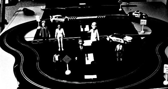
(a) capture under SS1

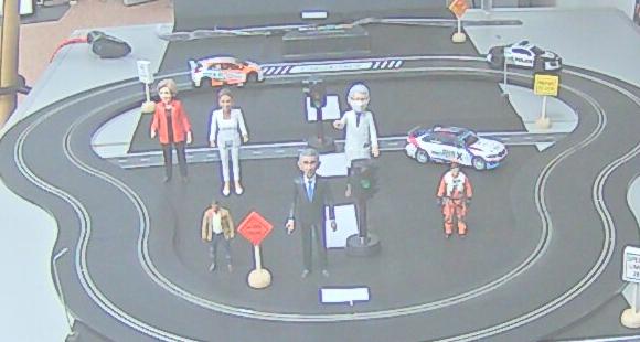
(b) capture under SS2

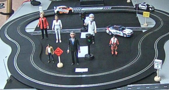
(c) CamTuner camera capture

Figure 12. Sample static & CamTuner camera captures.

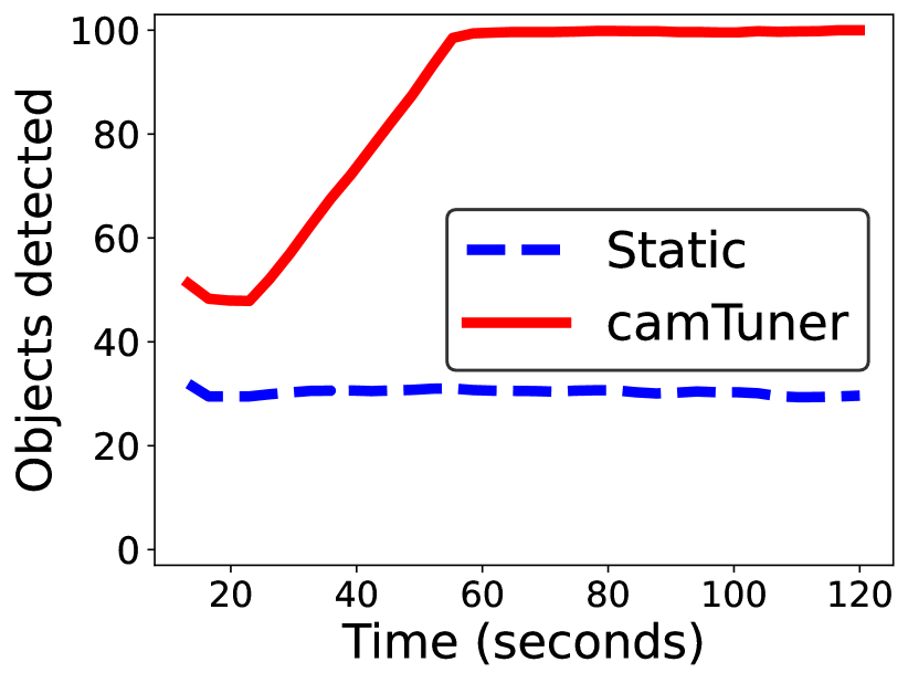
(a) suboptimal setting 1 (SS1)

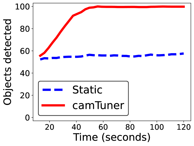
(b) suboptimal setting 2 (SS2)

Figure 13. CamTuner reaction to suboptimal settings (Normalized Moving average of total object detection is computed over last 100 frames, shown in Y axis.)

7.3. Real-world Deployment (Parking Lot)

To validate that similar accuracy improvement from video-playback in §7.1.2 is achieved in real-world deployment where the I-A parameters of the camera are continuously reconfigured by CamTuner, we evaluated our deployment of CamTuner at a large enterprise parking lot. The real-world deployment has two co-located cameras, as shown in Figure 14. One camera is part of the Baseline VAP (VAP 1) while the other camera is part of the CamTuner VAP (VAP 2). Both VAP deployments use Axis Q3505 MK II Network cameras, which upload the captured frames over 5G network to a remote edge-server (with a Xeon processor and an NVIDIA GPU) running the Efficientdet (tan2020efficientdet, ) object detection model to detect cars and persons in the parking lot. In VAP 2, the captured frames are also sent in parallel to CamTuner which runs on a low-end Intel-NUC box (with a 2.6 GHz Intel i7-6770HQ CPU). CamTuner is seeded with the same initially VC-trained RL agent as in §7.1.2 and it performs a few initial online exploration rounds and then starts exploitation and adjusts camera settings every 30 seconds. To evaluate the accuracy of the AUs in the VAPs, we ensure that both cameras view almost identical scenes at the same time.

We ran both VAPs side-by-side for 8 continuous hours in a day and recorded the videos from both VAPs. Since we want to manually inspect and validate the detections from both VAPs, we randomly picked detections for 5-minute spans during Morning and Evening time and compare car and person detections across the two VAPs.  Figure 15 shows the cumulative number of true-positive car and person detections.  Figure 15(a) and  Figure 15(c) show that CamTuner detects 2.2% (3) and 15.9% (146) additional persons than Baseline during Morning and Evening, respectively. CamTuner also detects 2.6% (861) and 4.2% (881) more cars than the Baseline VAP during Morning and Evening, respectively, as shown in Figure 15(b) and  Figure 15(d). Upon manual inspection of the videos, we confirmed that CamTuner does not have any false positive detections for car/person.

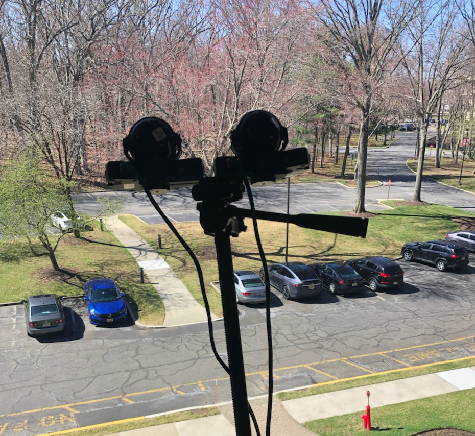
Figure 14. CamTuner real-world deployment setup.

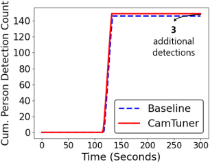
(a)

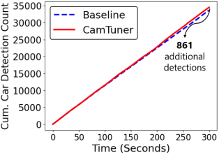
(b)

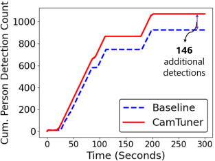
(c)

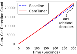
(d)

Figure 15. CamTuner performance in Parking lot.

7.4. 5G Use Case: Automatic Vehicle Collision Prediction (AVCP)

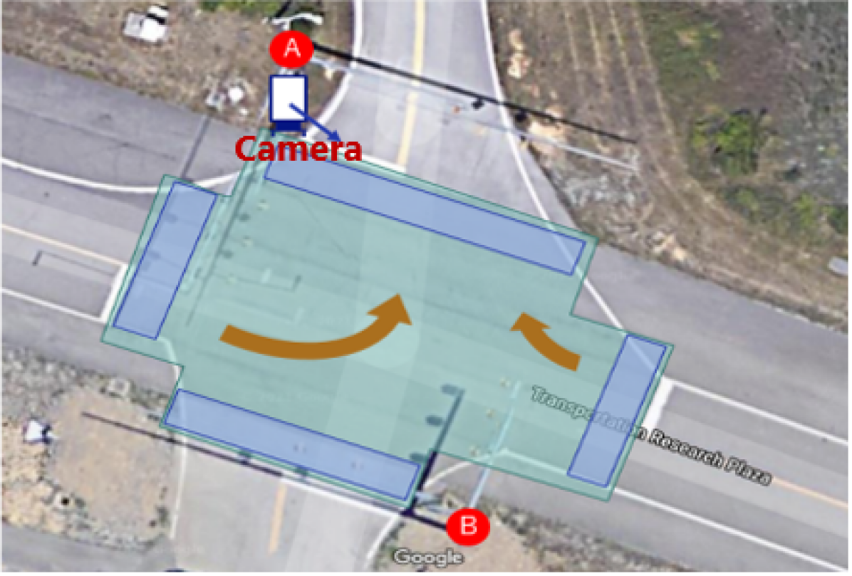
(a) Intersection

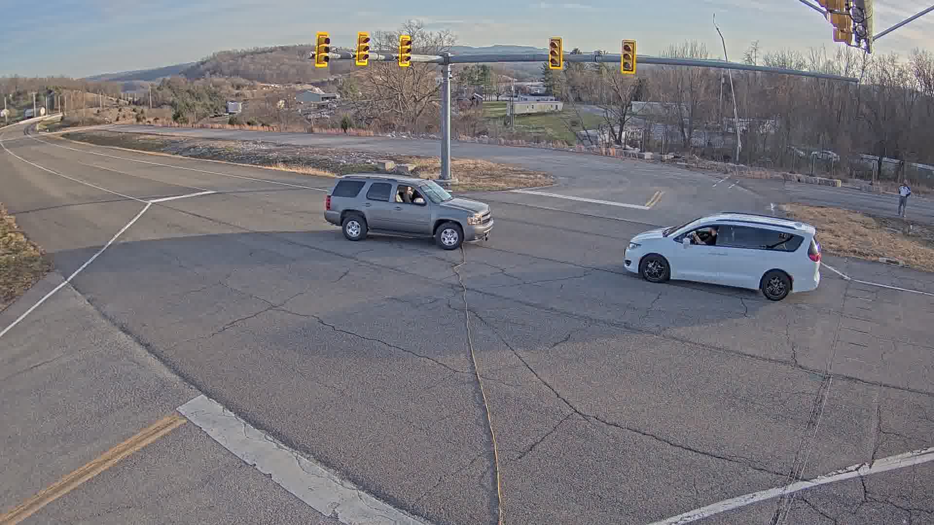
(b) Before accident

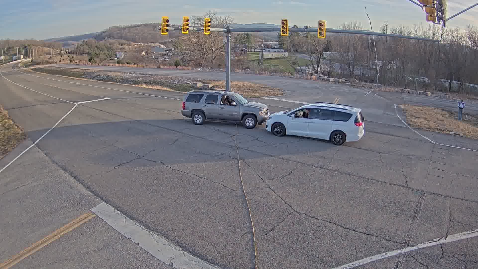
(c) Car accident

Figure 16. Car accident prevention scenario.

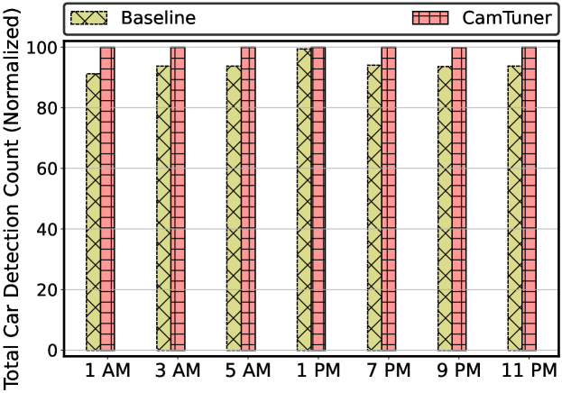
Figure 17. CamTuner performance in Accident Prevention scenario.

AVCP is an important use case in Intelligent Transportation Systems (ITS). This use case requires extremely low latency because it is very critical to predict collision and react almost instantaneously in order to prevent a potential life-threatening accident. In particular, low latency in the order of milliseconds is desired for this use case which can be achieved by using 5G, which promises ultra-reliable low latency communication (URLLC). In AVCP usecase, reliably detecting and tracking vehicles and pedestrians is one of the most critical building blocks; without this, the collision prediction won’t work properly and may lead to life-threatening accidents. CamTuner plays an important role in AVCP usecase, where it changes the camera settings dynamically in reaction to the environmental changes. Since the environment does not change within seconds, CamTuner’s quick (in the order of milliseconds) adjustment of camera setting improves the detection and tracking of vehicles and pedestrians at all times.

To evaluate this use case, we recorded a 1.5-minute-long car accident scenario, as shown in  Figure 16, at one of our customer sites that has a 5G smart traffic intersection testbed. We then used the experimental methodology described in §7.1.1 to emulate the same car accident scenario at 7 different hours (i.e., environmental conditions) of the same day, and running 2 VAPs (VAP 1 uses the default camera settings, denoted as Baseline and VAP 2 runs CamTuner) that detect cars using EfficientDet object detector.  Figure 17 shows that compared to VAP 1, VAP 2 using CamTuner detects 6.2% additional cars on average across the different hours, and as much as 9.7% (122) more cars at 1 AM.

7.5. System Performance

Since CamTuner runs in parallel with the AU, it does not add any additional latency to the VAP and hence the AU latency. In the following, we show that the normal online operation of CamTuner is light-weight, and the initial training phase using VC can explore each action extremely fast.

First, during online operation, each iteration of CamTuner involves three tasks: evaluating the AU-specific quality estimator, evaluating the Q-function by the SARSA agent, and changing the parameters of the physical camera. We run CamTuner on a low-end edge device, an Intel-NUC box equipped with a 2.6 GHz Intel i7-6770HQ CPU. The AU-specific quality estimator takes 40ms and the SARSA RL agent takes less than 1 ms to complete Q-function calculation and Q-table update. Since the two tasks can be pipelined with changing the physical camera settings which takes up to 200 ms on the AXIS Q3505 MK II Network camera we used, each iteration of CamTuner takes 200 ms, i.e., 5 iterations per second, and the average CPU utilization is only 15% with 150 MB memory footprint.

Next, we run the initial RL training phase on a high-end PC with a 3.70 GHz Intel(R) Xeon(R) W-2145 CPU and GeForce RTX 2080 GPU. During the one-hour training phase performed in §4, in each iteration of the RL exploration, VC takes 4 ms to output $f_{o}$, the quality estimator takes 10 ms, and the RL agent take less than 1 ms to evaluate the Q-function and update the Q-table, for a total of 15 ms. As a result, CamTuner can explore around 70 actions per second, which is 14X faster than using the physical camera. The CPU utilization in this case is steady at 60%.

7.6. Accuracy of Offline Trained Models

Finally, we evaluate the efficacy of two key components of CamTuner which are trained offline: VC and AU-specific analytics quality estimator model.

Table 4. Accuracy of VC.

Parameter	Brightness	Contrast	Color	Sharpness
		-Saturation
Mean error	$5.4\text{\,}\mathrm{\char 37\relax}$	$13.8\text{\,}\mathrm{\char 37\relax}$	$17.3\text{\,}\mathrm{\char 37\relax}$	$19.8\text{\,}\mathrm{\char 37\relax}$
Std. dev.	$1.7\text{\,}\mathrm{\char 37\relax}$	$4.3\text{\,}\mathrm{\char 37\relax}$	$9.6\text{\,}\mathrm{\char 37\relax}$	$8.1\text{\,}\mathrm{\char 37\relax}$

Virtual camera. VC is designed to render a frame taken at one time ($T_{1}$) to another time ($T_{2}$), as if the rendered frame were captured at time $T_{2}$. First, we trained VC in the offline profiling phase as discussed in §5.3 using a 24-hour long video obtained from one of our customer locations at an airport. To evaluate how well VC works online, we obtained several video snippets at 6 different hours of the day from the same camera. Next, we fed 1 video snippet $VS_{0}$ from one particular hour $H_{0}$ through VC which applies different digital transformation to generate 5 video snippets $VS_{j}$ corresponding to the hours of the other 5 videos. For each generated video snippet $VS_{j}$, we calculated the relative error of the metric tuple values of each frame in $VS_{j}$ relative to that of the corresponding original video frame and average such error across all the frames in $VS_{j}$ (over 37.5K frames). We obtained 5 VC error metric tuples for one video, each corresponding to the hour of the other 5 video snippets. We repeated the above experiment for the 5 other original video snippets to obtain a total of 30 VC error tuples.  Table 4 shows the mean error and standard deviation among all 30 VC error tuples. We observe that the average VC errors are 5.4%, 13.8%, 17.3%, and 9.8% for brightness, contrast, color-saturation and sharpness, respectively.

AU-specific analytics quality estimator.

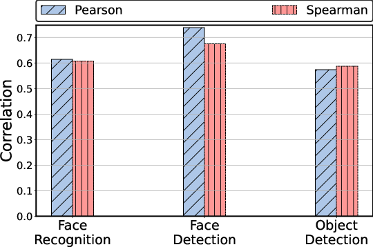
Figure 18. Analytics quality estimator performance.

Next, we evaluate the performance of AU-specific quality estimators. Since the AU-specific estimator is a lightweight model that predicts coarse-grained accuracy measure of the heavyweight DNN model (i.e., used in AU), it is not meaningful to compare its accuracy against the accuracy achieved by the heavyweight model (derived using ground truth). Instead, we measure the quality of the AU-specific quality estimator by measuring the Spearman and Pearson correlation between the two accuracies for three different AUs i.e. face-recognition, face-detection, and person-detection. First, we trained the three estimators through supervised learning as described in Section 5.2. To evaluate the face-recognition estimator, we used the celebA-validation dataset which contains 200 images (i.e., different from the 300 original training images used in Section 5.2) and their about 2 million variants from augmenting the original images using the python-pil image library (pil, ).  Figure 18 shows that the quality predicted by the face-recognition analytics quality estimator is strongly correlated with the output by the AU (both Pearson and Spearman correlation are greater than 0.6) (corr, ; corr_1, ).

To evaluate the face-detection quality estimator, we used annotated video frames from the olympics (niebles2010modeling, ) and HMDB datasets (Kuehne11, ) and their 4 million variants that were generated. To evaluate object-detection analytics quality estimator, we used labelled images (i.e., only consist car and person object classes) from the COCO dataset (lin2014microsoft, ) and their 7 million augmented variants  Figure 18 shows that there is a strong positive correlation between the measured mAP and IoU metric and the predicted quality estimate for both face-detection and object-detection AUs. In summary, the strong correlation between the prediction by the estimators and the actual quality of AUs based on ground truth, enables CamTuner’s RL agent to effectively tune camera parameters.

8. Related Work

Similar to our findings, Jang et al. (Jang2018ApplicationAwareIC, ) also show that environmental condition changes affect VAP, but their approach to adapt to such changes is to use different AUs depending on the environmental conditions, e.g., using Haar cascade for detection when lighting is sufficient and switch to HOG when environment gets darker. Since there could be several reasons for change in environment as discussed in §3.1, developing an AU for every kind of environment is not feasible. In contrast, CamTuner takes a different approach where the AU is fixed and camera settings are adjusted to adapt to environmental changes.

Several works investigate tuning parameters of a VAP after camera capture and before sending it to an AU or changing the AU based on the input video content. Videostorm (201465, ), Chameleon (jiang2018chameleon, ), and Awstream (zhang2018awstream, ) tune the after-capture video stream parameters such as frames-per-second or frame resolution to ensure efficient resource usage while processing video analytics queries at scale. In contrast, CamTuner dynamically tunes camera parameters to improve the AU accuracy of VAPs.

More recent work, e.g., Focus (222587, ), NoScope (10.14778/3137628.3137664, ), Ekya (padmanabhantowards, ), and AMS (khani2020real, ), studied how to adapt AU model parameters based on captured video content. Such an approach requires additional GPU resources for periodic model retraining and is also less reactive to video content changes. In contrast, CamTuner quickly adapts the camera parameters in real-time according to environmental changes.

Several frame filtering techniques on edge devices (MLSYS2019_85d8ce59, ; paul2021aqua, ; chen2015glimpse, ; li2020reducto, ) can work in conjunction with CamTuner and potentially further improve CamTuner’s performance. Our AU-specific analytics quality estimator shares similar goal as the AQuA-quality estimator (paul2021aqua, ) but differs in that CamTuner’s quality estimator performs quality estimation that is specific to each AU, while AQuA performs much more coarse-grained AU-agnostic image quality estimation.

There is a large body of work on configuring the Image Signal Processing pipeline (ISP) in cameras to improve human-perceived quality of images from the cameras  (wu2019visionisp, ; liu2020joint, ; diamond2021dirty, ; nishimura2019automatic, ). In contrast, we study dynamic camera parameter tuning to optimize the accuracy of VAPs.

9. Future Work

Our first demonstration in this paper of how NAUTO camera parameters can be dynamically tuned to enhance video analytics accuracy opens up many avenues for future research. Here, we consider only a subset of NAUTO camera parameters related to image appearance but there are several other NAUTO parameters such as max exposure time, maximum gain, and defog effect (listed in  Table 1) that can also be dynamically tuned to enhance video analytics accuracy. In our future work, we plan to study the impact of dynamically tuning these other camera parameters as well.

Current CamTuner design tunes NAUTO camera parameters in order to enhance video analytics accuracy of a single AU. However, in a typical camera deployment there could be multiple AUs sharing a single video stream. For example, in an enterprise building entrance where a surveillance camera is deployed, it is common to have separate AUs including authorization for the car and people entering, counting number of cars and people entering/leaving, etc. that all need to run on the same camera stream. In our future work, we will study how to tune camera parameters in order to simultaneously enhance the accuracy for multiple AUs.

10. Conclusion

In this paper, we presented the design and evaluation of CamTuner, to our knowledge the first adaptive VAP framework that adaptively learns the best setting for its NAUTO camera parameters deployed in the field in reaction to environmental changes to enhance AU accuracy. Our controlled experiments and real-world VAP deployment show that compared to a VAP using the default camera setting, CamTuner allows the VAP to detect 15.9% additional persons and 2.6%–4.2% additional cars (without any false positives) in a large enterprise large parking lot and 9.7% additional cars in a 5G smart traffic intersection scenario. CamTuner dynamically determines how to tune IP camera parameters, which can be executed either directly inside the camera via the exposed REST APIs for remotely configuring the camera setting, or via digital transformation after camera capture, e.g., for cameras that do not expose such APIs. Furthermore, we believe CamTuner’s design and its key components, Virtual Camera and light-weight AU-specific analytics quality estimators, can be applied to dynamically tune other complex sensors such as depth and thermal cameras.

References

- [1] NATS: Connective Technology for Adaptive Edge & Distributed Systems. https://nats.io/.
- [2] Open Source Computer Vision Library. https://opencv.org/.
- [3] Zeromq: An open-source universal messaging library. https://zeromq.org/.
- [4] Vp9. https://www.webmproject.org/vp9/, 2017.
- [5] x264. http://www.videolan.org/developers/x264.html, 2021.
- [6] B. E. Bayer. Color imaging array, July 20 1976. US Patent 3,971,065.
- [7] S. Bezryadin, P. Bourov, and D. Ilinih. Brightness calculation in digital image processing. In International symposium on technologies for digital photo fulfillment, volume 2007, pages 10–15. Society for Imaging Science and Technology, 2007.
- [8] T. BMJ. correlation-and-regression. https://www.bmj.com/about-bmj/resources-readers/publications/statistics-square-one/11-correlation-and-regression, 2019.
- [9] C. Canel, T. Kim, G. Zhou, C. Li, H. Lim, D. G. Andersen, M. Kaminsky, and S. Dulloor. Scaling Video Analytics on Constrained Edge Nodes. In A. Talwalkar, V. Smith, and M. Zaharia, editors, Proceedings of Machine Learning and Systems, volume 1, pages 406–417, 2019.
- [10] E. H. Chen, P. Röthig, J. Zeisler, and D. Burschka. Investigating Low Level Features in CNN for Traffic Sign Detection and Recognition. In 2019 IEEE Intelligent Transportation Systems Conference (ITSC), pages 325–332, 2019.
- [11] T. Y.-H. Chen, L. Ravindranath, S. Deng, P. Bahl, and H. Balakrishnan. Glimpse: Continuous, real-time object recognition on mobile devices. In Proceedings of the 13th ACM Conference on Embedded Networked Sensor Systems, pages 155–168, 2015.
- [12] CISCO. Cisco Video Surveillance IP Cameras. https://www.cisco.com/c/en/us/products/physical-security/video-surveillance-ip-cameras/index.html.
- [13] A. Clark and Contributors. Pillow library. https://pillow.readthedocs.io/en/stable/.
- [14] CNET. How 5G aims to end network latency. CNET_5G_network_latency_time, 2019.
- [15] cocoapi github. pycocotools. https://github.com/cocodataset/cocoapi/tree/master/PythonAPI/pycocotools.
- [16] A. Communication. AXIS Network Cameras. https://www.axis.com/products/network-cameras.
- [17] K. De and V. Masilamani. Image sharpness measure for blurred images in frequency domain. Procedia Engineering, 64:149–158, 2013.
- [18] J. Deng, J. Guo, Z. Yuxiang, J. Yu, I. Kotsia, and S. Zafeiriou. RetinaFace: Single-stage Dense Face Localisation in the Wild. In arxiv, 2019.
- [19] S. Diamond, V. Sitzmann, F. Julca-Aguilar, S. Boyd, G. Wetzstein, and F. Heide. Dirty Pixels: Towards End-to-end Image Processing and Perception. ACM Transactions on Graphics (TOG), 40(3):1–15, 2021.
- [20] V. Gaikwad and R. Rake. Video Analytics Market Statistics: 2027, 2021.
- [21] A. Gupta, A. Anpalagan, L. Guan, and A. S. Khwaja. Deep learning for object detection and scene perception in self-driving cars: Survey, challenges, and open issues. Array, 10:100057, 2021.
- [22] D. Hasler and S. E. Suesstrunk. Measuring colorfulness in natural images. In Human vision and electronic imaging VIII, volume 5007, pages 87–95. International Society for Optics and Photonics, 2003.
- [23] K. Hsieh, G. Ananthanarayanan, P. Bodik, S. Venkataraman, P. Bahl, M. Philipose, P. B. Gibbons, and O. Mutlu. Focus: Querying Large Video Datasets with Low Latency and Low Cost. In 13th USENIX Symposium on Operating Systems Design and Implementation (OSDI 18), pages 269–286, Carlsbad, CA, Oct. 2018. USENIX Association.
- [24] i PRO. i-PRO Network Camera. http://i-pro.com/global/en/surveillance.
- [25] S. Y. Jang, Y. Lee, B. Shin, and D. Lee. Application-Aware IoT Camera Virtualization for Video Analytics Edge Computing. 2018 IEEE/ACM Symposium on Edge Computing (SEC), pages 132–144, 2018.
- [26] J. Jiang, G. Ananthanarayanan, P. Bodik, S. Sen, and I. Stoica. Chameleon: scalable adaptation of video analytics. In Proceedings of the 2018 Conference of the ACM Special Interest Group on Data Communication, pages 253–266, 2018.
- [27] G. Jocher, A. Chaurasia, A. Stoken, J. Borovec, NanoCode012, Y. Kwon, TaoXie, J. Fang, imyhxy, K. Michael, Lorna, A. V, D. Montes, J. Nadar, Laughing, tkianai, yxNONG, P. Skalski, Z. Wang, A. Hogan, C. Fati, L. Mammana, AlexWang1900, D. Patel, D. Yiwei, F. You, J. Hajek, L. Diaconu, and M. T. Minh. ultralytics/yolov5: v6.1 - TensorRT, TensorFlow Edge TPU and OpenVINO Export and Inference, Feb. 2022.
- [28] D. Kang, J. Emmons, F. Abuzaid, P. Bailis, and M. Zaharia. NoScope: Optimizing Neural Network Queries over Video at Scale. Proc. VLDB Endow., 10(11):1586–1597, Aug. 2017.
- [29] M. Khani, P. Hamadanian, A. Nasr-Esfahany, and M. Alizadeh. Real-Time Video Inference on Edge Devices via Adaptive Model Streaming. arXiv preprint arXiv:2006.06628, 2020.
- [30] D. P. Kingma and J. Ba. Adam: A method for stochastic optimization. arXiv preprint arXiv:1412.6980, 2014.
- [31] A. Krizhevsky, I. Sutskever, and G. E. Hinton. Imagenet classification with deep convolutional neural networks. In Advances in neural information processing systems, pages 1097–1105, 2012.
- [32] H. Kuehne, H. Jhuang, E. Garrote, T. Poggio, and T. Serre. HMDB: a large video database for human motion recognition. In Proceedings of the International Conference on Computer Vision (ICCV), 2011.
- [33] Y. Li, A. Padmanabhan, P. Zhao, Y. Wang, G. H. Xu, and R. Netravali. Reducto: On-Camera Filtering for Resource-Efficient Real-Time Video Analytics. In Proceedings of the Annual conference of the ACM Special Interest Group on Data Communication on the applications, technologies, architectures, and protocols for computer communication, pages 359–376, 2020.
- [34] T.-Y. Lin, M. Maire, S. Belongie, J. Hays, P. Perona, D. Ramanan, P. Dollár, and C. L. Zitnick. Microsoft coco: Common objects in context. In European conference on computer vision, pages 740–755. Springer, 2014.
- [35] L. Liu, X. Jia, J. Liu, and Q. Tian. Joint demosaicing and denoising with self guidance. In Proceedings of the IEEE/CVF Conference on Computer Vision and Pattern Recognition, pages 2240–2249, 2020.
- [36] Z. Liu, P. Luo, X. Wang, and X. Tang. Deep Learning Face Attributes in the Wild. In Proceedings of International Conference on Computer Vision (ICCV), December 2015.
- [37] A. Mittal, A. K. Moorthy, and A. C. Bovik. No-reference image quality assessment in the spatial domain. IEEE Transactions on image processing, 21(12):4695–4708, 2012.
- [38] J. C. Niebles, C.-W. Chen, and L. Fei-Fei. Modeling temporal structure of decomposable motion segments for activity classification. In European conference on computer vision, pages 392–405. Springer, 2010.
- [39] J. Nishimura, T. Gerasimow, S. Rao, A. Sutic, C.-T. Wu, and G. Michael. Automatic ISP image quality tuning using non-linear optimization, 2019.
- [40] A. Padmanabhan, A. P. Iyer, G. Ananthanarayanan, Y. Shu, N. Karianakis, G. H. Xu, and R. Netravali. Towards Memory-Efficient Inference in Edge Video Analytics.
- [41] S. Paul, U. Drolia, Y. C. Hu, and S. T. Chakradhar. Aqua: Analytical quality assessment for optimizing video analytics systems. In 2021 IEEE/ACM Symposium on Edge Computing (SEC), pages 135–147. IEEE, 2021.
- [42] E. Peli. Contrast in complex images. JOSA A, 7(10):2032–2040, 1990.
- [43] Qualcomm. How 5G low latency improves your mobile experiences. Qualcomm_5G_low-latency_improves_mobile_experience, 2019.
- [44] R. Ramanath, W. E. Snyder, Y. Yoo, and M. S. Drew. Color image processing pipeline. IEEE Signal Processing Magazine, 22(1):34–43, 2005.
- [45] Statisticssolutions. Pearson correlation coefficient. https://www.statisticssolutions.com/free-resources/directory-of-statistical-analyses/pearsons-correlation-coefficient/, 2019.
- [46] R. S. Sutton, A. G. Barto, et al. Introduction to reinforcement learning, volume 135. MIT press Cambridge, 1998.
- [47] C. Szegedy, V. Vanhoucke, S. Ioffe, J. Shlens, and Z. Wojna. Rethinking the Inception Architecture for Computer Vision. In 2016 IEEE Conference on Computer Vision and Pattern Recognition (CVPR), pages 2818–2826, 2016.
- [48] M. Tan, R. Pang, and Q. V. Le. Efficientdet: Scalable and efficient object detection. In Proceedings of the IEEE/CVF conference on computer vision and pattern recognition, pages 10781–10790, 2020.
- [49] C. J. C. H. Watkins and P. Dayan. Q-learning. In Machine Learning, pages 279–292, 1992.
- [50] M. Wiering and J. Schmidhuber. Fast Online q(). Machine Learning, 33(1):105–115, Oct 1998.
- [51] C.-T. Wu, L. F. Isikdogan, S. Rao, B. Nayak, T. Gerasimow, A. Sutic, L. Ain-kedem, and G. Michael. VisionISP: Repurposing the image signal processor for computer vision applications. In 2019 IEEE International Conference on Image Processing (ICIP), pages 4624–4628. IEEE, 2019.
- [52] B. Zhang, X. Jin, S. Ratnasamy, J. Wawrzynek, and E. A. Lee. Awstream: Adaptive wide-area streaming analytics. In Proceedings of the 2018 Conference of the ACM Special Interest Group on Data Communication, pages 236–252, 2018.
- [53] H. Zhang, G. Ananthanarayanan, P. Bodik, M. Philipose, P. Bahl, and M. J. Freedman. Live Video Analytics at Scale with Approximation and Delay-Tolerance. In 14th USENIX Symposium on Networked Systems Design and Implementation (NSDI 17), pages 377–392, Boston, MA, Mar. 2017. USENIX Association.