Likelihood-Free Frequentist Inference: Bridging Classical Statistics and
Machine Learning for Reliable
Simulator-Based InferenceThis work was supported in part by NSF DMS-2053804, NSF PHY-2020295, and the C3.ai Digital Transformation Institute. RI is grateful for the financial support of CNPq (309607/2020-5 and 422705/2021-7) and FAPESP (2019/11321-9 and 2023/07068-1).

Abstract

Many areas of science make extensive use of computer simulators that implicitly encode intractable likelihood functions of complex systems. Classical statistical methods are poorly suited for these so-called likelihood-free inference (LFI) settings, especially outside asymptotic and low-dimensional regimes. At the same time, traditional LFI methods – such as Approximate Bayesian Computation or more recent machine learning techniques – do not guarantee confidence sets with nominal coverage in general settings (i.e., with high-dimensional data, finite sample sizes, and for any parameter value). In addition, there are no diagnostic tools to check the empirical coverage of confidence sets provided by such methods across the entire parameter space. In this work, we propose a unified and modular inference framework that bridges classical statistics and modern machine learning providing (i) a practical approach to the Neyman construction of confidence sets with frequentist finite-sample coverage for any value of the unknown parameters; and (ii) interpretable diagnostics that estimate the empirical coverage across the entire parameter space. We refer to the general framework as likelihood-free frequentist inference (LF2I). Any method that defines a test statistic can leverage LF2I to create valid confidence sets and diagnostics without costly Monte Carlo samples at fixed parameter settings. We study the power of two likelihood-based test statistics (ACORE and BFF) and demonstrate their empirical performance on high-dimensional, complex data. Code is available at https://github.com/lee-group-cmu/lf2i.

t1Equal Contribution

1 Introduction

Hypothesis testing and uncertainty quantification are the hallmarks of scientific inference. Methods that achieve good statistical performance (e.g., high power) often rely on being able to explicitly evaluate a likelihood function, which relates parameters of the data-generating process to observed data. However, in many areas of science and engineering, complex phenomena are modeled by forward simulators that implicitly define a likelihood function. For example, given input parameters $\theta$ from some parameter space $\Theta$, a stochastic model $F_{\theta}$ may encode the interaction of atoms or elementary particles , or the transport of radiation through the atmosphere or through matter in the Universe by combining deterministic dynamics with random fluctuations and measurement errors, to produce synthetic data ${\mathbf{X}}$.

Simulation-based inference with an intractable likelihood is commonly referred to as likelihood-free inference (LFI). The most well-known approach to LFI is Approximate Bayesian Computation (ABC; see [6, 63, 81] for a review). These methods use simulations sufficiently close to the observed data $D=\left\{{\mathbf{x}}_{1}^{\text{obs}},\ldots,{\mathbf{x}}_{n}^{\text{obs}}\right\}$ to infer the underlying parameters, or more precisely, the posterior distribution $p(\theta|D)$. Recently, the arsenal of LFI methods has been expanded with new machine learning algorithms (such as neural density estimators) that instead use the output from simulators as training data; see Section 1.1, “Likelihood-free inference via machine learning”. The objective here is to learn a “surrogate model” or approximation of the likelihood $p(D|\theta)$ or posterior $p(\theta|D)$. The surrogate model, rather than the simulations themselves, is then used for inference.

Machine-learning (ML) based methods have revolutionized LFI in terms of the complexity and dimensionality of the problems that can be tackled (see [23] for a recent review). Nevertheless, neither ABC nor ML-based LFI approaches guarantee confidence sets with frequentist coverage in general settings. Suppose that we have a high-fidelity simulator $F_{\theta}$, which implicitly encodes the likelihood, and that we observe data ${\mathcal{D}}$ of finite sample size $n$. The first open problem is finding a practical procedure to construct a $(1-\alpha)$ confidence set $R({\mathcal{D}})$ with the nominal coverage

$$\mathbb{P}_{\mathcal{D}|\theta}\left(\theta\in R({\mathcal{D}})\right)=1-\alpha,$$ (1)

where $\alpha\in(0,1)$, regardless of the true value of the unknown parameter $\theta\in\Theta$ and of the number of observations $n$. Monte Carlo and bootstrap procedures are computationally infeasible for continuous parameter spaces $\Theta$, and large-sample theory does not apply when, e.g., $n=1$. The second open problem is finding practical and interpretable procedures to check that the empirical coverage of the constructed sets $R({\mathcal{D}})$ is indeed close to (and no smaller than) $1-\alpha$ for any $\theta\in\Theta$ (again, without resorting to costly Monte Carlo simulations at fixed parameter settings on a fine grid in parameter space $\Theta$ [18, Section 13]).

Novelty and Significance

In this paper, we introduce a fully modular statistical framework for LFI which unifies classical statistics with modern machine learning (e.g., deep generative models, neural network classifiers, and nonparametric quantile regression) to (i) construct finite-sample confidence sets with nominal coverage for any value of the unknown parameters, and (ii) provide interpretable diagnostics to assess empirical coverage across the entire parameter space. We refer to the framework as likelihood-free frequentist inference (LF2I). The approach is fully nonparametric, and targets complex data settings (e.g., high-dimensional data ${\mathbf{X}}$ with nonlinear structure, intractable likelihood models, small sample size $n$ or unknown limiting distribution of test statistic), which are directly relevant to scientific applications in several domains, such as, for example, high-energy physics and astronomy. Section 1.1 describes how LF2I is related to other work.

Our Approach

At the heart of LF2I is the Neyman construction of confidence sets (Figure 2), albeit applied to a setting where the distribution of the test statistic is unknown. The construction of frequentist confidence sets with nominal coverage has a long history in statistics [36, 69], with the equivalence between tests and confidence sets formalized in [70]. Classical statistical procedures (including the Neyman construction) have had a remarkable impact on scientific fields such as high-energy physics (see Section 1.1), but most simulator-based methods do not have theoretical guarantees on validity and power of Neyman confidence sets beyond low-dimensional data settings and large-sample theory assumptions [35].

What makes the Neyman construction difficult to implement for LFI is not only that one cannot evaluate the likelihood, but also that one needs to consider the hypothesis test $H_{0,\theta_{0}}:\theta=\theta_{0}$ for every $\theta_{0}\in\Theta$. Monte Carlo and bootstrap approaches to hypothesis testing typically estimate critical values and significance probabilities (p-values) from a batch of simulations generated at the null value $\theta_{0}$ (see, e.g., [62] and [88]). Such an approach is computationally inefficient and infeasible in higher-dimensional parameter spaces, because the Neyman construction would then require a separate MC or bootstrap batch at each $\theta_{0}$ on a fine grid over the parameter space. Hence, in practice, Neyman inversions rely either on parametric model assumptions or asymptotic theory [71, 92]. A standard example for this is the likelihood-ratio (LR) statistic, which is often assumed to follow a $\chi^{2}$ distribution. There are however at least two cases where this assumption breaks down: when the statistical model is irregular (see Section 6.1 for a Gaussian mixture model with intractable null distribution), and when the sample size $n$ is small. Note that irregular models, high-dimensional data, and sample sizes as small as $n=1$ are common in physics; recent examples include estimating the momentum ($\theta$) of a muon from the energy it deposited in a finely segmented calorimeter (${\mathbf{X}}={\mathcal{D}}$) [53], and estimating the mass of a galaxy cluster ($\theta$) from velocities and projected radial distances (${\mathbf{X}}={\mathcal{D}}$) for a particular line-of-sight of the observer relative the galaxy cluster [46]. In this work, we ask how we can quickly and accurately estimate critical values and coverage across the entire parameter space, when we do not know the distribution of the test statistic and cannot rely on large-sample approximations.

The main idea behind LF2I is that key quantities of interest in frequentist statistical inference – test statistics, critical values, p-values and coverage of the confidence set – are conditional distribution functions of the (unknown) parameters $\theta$, and generally vary smoothly over the parameter space $\Theta$. As a result, one can leverage machine learning methods and data simulated in the neighborhood of a parameter to improve estimates of quantities of interest with fewer total simulations. Figure 1 illustrates the general LF2I inference machinery, which is composed of three modular branches with separate functionalities:

• The “test statistic” branch (Figure 1 center and Section 3.2) estimates a test statistic $\lambda({\mathcal{D}};\theta)$ from a simulated set ${\mathcal{T}}$. In this paper, we study the theoretical and empirical performance of LF2I confidence sets derived from likelihood-based test statistics learned via the odds function ${\mathbb{O}}({\mathbf{X}};\theta)$ (Equation 7) from data ${\mathbf{X}}$ drawn from a simulator $F_{\theta}$ and a reference distribution $G$.

• The “calibration” branch (Figure 1 left and Section 3.3) draws a second sample $\mathcal{T}^{{}^{\prime}}$ to estimate the critical value $C_{\theta_{0}}$ for every level-$\alpha$ test of $H_{0,\theta_{0}}:\theta=\theta_{0}$ vs. $H_{1,\theta_{0}}:\theta\neq\theta_{0}$ via quantile regression of the estimated test statistic $\lambda({\mathcal{D}};\theta_{0})$ on $\theta_{0}\in\Theta$. Once we have estimated the conditional quantile function $\widehat{C}_{\theta_{0}}$, we can directly construct Neyman confidence sets

  $$\widehat{R}({\mathcal{D}}):=\left\{\theta\in\Theta\,\middle|\,\lambda({\mathcal{D}};\theta)\geq\widehat{C}_{\theta}\right\}$$ (2)

  that have approximate $(1-\alpha)$ finite-$n$ coverage, no matter what the value of the true parameter $\theta\in\Theta$ is. LF2I with critical values is amortized, meaning that once trained it can be evaluated on an arbitrary number of observations $D$. Alternatively, we can estimate p-values $p(D;\theta_{0})$ for every test at $\theta=\theta_{0}$ with observed data $D$.

• The “diagnostics” branch (Figure 1 right and Section 3.4) draws a third sample $\mathcal{T}^{{}^{\prime\prime}}$ to assess the empirical coverage ${\mathbb{P}}_{{\mathcal{D}}|\theta}(\theta\in\widehat{R}({\mathcal{D}}))$ of the constructed confidence sets $\widehat{R}({\mathcal{D}})$ for every $\theta\in\Theta$ by regressing the indicator variable $W:=\mathbb{I}(\lambda({\mathcal{D}};\theta)\geq\widehat{C}_{\theta})$ on $\theta$. That is, this procedure checks whether the constructed sets are indeed valid regardless of the true value of $\theta$. The diagnostics branch is not part of the inference procedure itself, but it is provided to ensure good statistical practice via an independent assessment of the claimed properties of the final model.

The LF2I machinery for constructing and assessing confidence sets with finite-$n$ coverage was first proposed in a short conference proceeding [26]. The preliminary version was called ACORE for “Approximate Computation via Odds Ratio Estimation”, and is based on a test statistic that maximizes the odds over the parameter space. When the odds function is well-estimated, the ACORE statistic (Equation 8) is the same as the well-known likelihood ratio statistic. In this paper, we study the statistical and computational properties of the general LF2I framework, while also introducing a new test statistic – the Bayesian Frequentist Factor (BFF) – which is the Bayes Factor [49, 50] treated as a frequentist test statistic. We show that validity in LF2I only depends on how well we calibrate, while power depends on how we define the test statistic and on how well we estimate it. In addition to new theoretical results, we present experiments that compare LF2I with approaches using Monte Carlo methods or Wilks’ theorem (Section 6.1), and illustrate how our diagnostics can help scientists in choosing the best approach for handling nuisance parameters (Section 6.2). Finally, we showcase LF2I confidence sets and diagnostics on a high-dimensional intractable high-energy physics experiment where ABC approaches do not achieve the correct coverage level and are also computationally infeasible (Section 6.3).

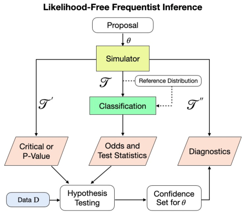
Figure 1: The three-branch fully modular framework for likelihood-free frequentist inference (LF2I). Center branch: Draw a sample ${\mathcal{T}}$ of size $B$ from the simulator to estimate an arbitrary test statistic $\lambda({\mathcal{D}};\theta)$. Here we show how to do so by estimating the likelihood via the odds function $\mathbb{O}({\mathbf{X}};\theta)$. Left branch: Draw a second sample ${\mathcal{T}}^{\prime}$ of size $B^{\prime}$ to estimate the critical values $C_{\theta}$ or p-values $p({\mathcal{D}};\theta)$ for all $\theta\in\Theta$. Left $+$ Center: Once data $D$ are observed, we can construct confidence sets $\widehat{R}(D)$ with finite-$n$ validity according to Equation 12. Right branch: The LF2I diagnostics branch independently checks whether the coverage ${\mathbb{P}}_{{\mathcal{D}}|\theta}(\theta\in\widehat{R}({\mathcal{D}}))$ of the confidence set is indeed correct across the entire parameter space.

1.1 Relation to Other Work and Our Contribution

Classical statistical inference in high-energy physics (HEP)

LF2I is inspired by pioneering work in HEP that adopted classical hypothesis tests and Neyman confidence sets for the discovery of new physics [35, 21, 1, 11, 22]. Our work grew from the discussion in HEP regarding theory and practice, and open problems such as how to efficiently construct Neyman confidence sets for general settings [21], how to assess coverage across the parameter space without costly Monte Carlo simulations [18], and how to choose hybrid techniques in practice [17]. This paper proposes a general approach to solve the above-mentioned open problems with a modular framework that can be adapted to fit the data at hand.

Universal inference

Recently, [90] proposed a “universal” inference test statistic for constructing valid confidence sets and hypothesis tests with finite-sample guarantees without regularity conditions. The assumptions are that the likelihood $\mathcal{L}(\mathcal{D};\theta)$ is known and that one can compute the maximum likelihood estimator (MLE). Our LF2I framework does not require a tractable likelihood, but it assumes that we have regression methods that can estimate the chosen test statistic and its critical values. In tractable likelihood settings where both universal inference and LF2I apply, the LF2I approach leads to more powerful tests than universal inference (see, e.g., Figure 10 in Supplementary Material).

Likelihood-free inference via machine learning

Recent LFI methods have been using simulators output as training data to learn surrogate models for inference; see [23] for a review. These techniques use synthetic data simulated across the parameter space to directly estimate key quantities, such as:

1. posteriors $p(\theta|{\mathbf{x}})$ [8, 64, 72, 60, 39, 13, 48, 77];

2. likelihoods $p({\mathbf{x}}|\theta)$ [93, 67, 91, 40, 33, 59, 74, 75, 51]; or

3. density ratios, such as the likelihood-to-marginal ratio $p({\mathbf{x}}|\theta)/p({\mathbf{x}})$ [47, 85, 44, 32], the likelihood ratio $p({\mathbf{x}}|\theta_{1})/p({\mathbf{x}}|\theta_{2})$ for $\theta_{1},\theta_{2}\in\Theta$ [24, 10] or the profile-likelihood ratio [42].

Recently, there have also been works that directly predict parameters $\theta$ of intractable models using neural networks [37, 56] (that is, they do not estimate posteriors, likelihoods or density ratios). In addition, new methods such as normalizing flows [73] and other neural density estimators are revolutionizing LFI in terms of sample efficiency and capacity, and will continue to do so.

Nonetheless, although the goal of LFI is inference on the unknown parameters $\theta$, it remains an open question whether a given LFI algorithm produces reliable measures of uncertainty. Current LFI methods do not guarantee validity and power for finite number of observations (without costly Monte Carlo samples at fixed parameter values), nor provide practical diagnostics for assessing coverage across the entire parameter space (when the true solution is not known). Our framework can lend good statistical properties and theoretical guarantees of nominal finite-$n$ coverage to any LFI algorithm that computes a “test statistic”; that is, a measure of how well observed data fits the conjecture that the true parameter $\theta$ has a certain value $\theta_{0}$. Finally, our diagnostics branch can also be used to check whether other LFI approaches (including ABC and posterior methods, which compute credible regions, and [86], which is based on confidence distributions) have good frequentist coverage properties, and pinpoint regions of the parameter space where they might be over- or under-confident.

Simulation-Based Calibration of Bayesian Posterior Distributions

In Bayesian inference, the posterior distribution $\pi(\theta|{\mathbf{x}})$ is fundamental for quantifying uncertainty about the parameter $\theta$ given the data ${\mathbf{x}}$. Recent methods have been developed to assess the quality of estimated posterior distributions; that is, assessing whether an estimate $\widehat{\pi}(\theta|{\mathbf{x}})$ is consistent with the posterior distribution $\pi(\theta|{\mathbf{x}})$ implied by the assumed prior and likelihood [27, 95, 28, 58, 55]. The calibration in LF2I is fundamentally different: Even if posteriors are calibrated in the sense that $\widehat{\pi}(\theta|{\mathbf{x}})=\pi(\theta|{\mathbf{x}})$ for every ${\mathbf{x}}$ and $\theta$, confidence sets derived from it will not necessarily have the correct empirical coverage (according to Eq.1). LF2I is agnostic to the choice of the test statistic (for instance, whether the test statistic is formed from likelihoods or posteriors [65]), and provides guarantees of how well we are able to constrain the true parameters of interest regardless of the choice of the prior or proposal distribution $\pi(\theta)$.

2 Statistical Inference in a Traditional Setting

We now review the Neyman construction of confidence sets and the definitions of likelihood ratio and Bayes factor, before moving on to the details of the LF2I framework and its two instances presented in this work: ACORE and BFF.

Equivalence of Tests and Confidence Sets

A classical approach to constructing a confidence set for an unknown parameter $\theta\in\Theta$ is to invert a series of hypothesis tests [70]. Suppose that for each possible value $\theta_{0}\in\Theta$, there is a level-$\alpha$ test $\delta_{\theta_{0}}$ of

$$H_{0,\theta_{0}}:\theta=\theta_{0}\ \ \mbox{versus}\ \ H_{1,\theta_{0}}:\theta\neq\theta_{0}.$$ (3)

That is, a test $\delta_{\theta_{0}}$ where the type I error (the probability of erroneously rejecting a true null hypothesis $H_{0,\theta_{0}}$) is no larger than $\alpha$. For observed data ${\mathcal{D}}=D$, let $R(D)$ be the set of all parameter values $\theta_{0}\in\Theta$ for which the test $\delta_{\theta_{0}}$ does not reject $H_{0,\theta_{0}}$. Then, by construction, the random set $R({\mathcal{D}})$ satisfies

$${\mathbb{P}}_{{\mathcal{D}}|\theta}\left(\theta\in R({\mathcal{D}})\right)\geq 1-\alpha\quad\forall\theta\in\Theta,$$

which makes it a $(1-\alpha)$ confidence set for $\theta$. Similarly, we can define tests with a desired significance level by inverting a confidence set with a certain coverage.

Likelihood Ratio Test

A general form of hypothesis tests that often leads to high power is the likelihood ratio test (LRT). Consider testing

$$H_{0}:\theta\in\Theta_{0}\ \ \mbox{versus}\ \ H_{1}:\theta\in\Theta_{1},$$ (4)

where $\Theta_{1}=\Theta\setminus\Theta_{0}$. For the likelihood ratio (LR) statistic,

$$\text{LR}({\mathcal{D}};\Theta_{0})=\log\frac{\sup_{\theta\in\Theta_{0}}\mathcal{L}({\mathcal{D}};\theta)}{\sup_{\theta\in\Theta}\mathcal{L}({\mathcal{D}};\theta)},$$ (5)

the LRT of hypotheses (4) rejects $H_{0}$ when $\text{LR}(D;\Theta_{0})<C$ for some constant $C$. Figure 2 illustrates the construction of confidence sets for $\theta$ from level $\alpha$ likelihood ratio tests (3). The critical value for each such test $\delta_{\theta_{0}}$ is $C_{\theta_{0}}=\sup\left\{C:{\mathbb{P}}_{{\mathcal{D}}|\theta_{0}}\left(\text{LR}({\mathcal{D}};\theta_{0})<C\right)\leq\alpha\right\}$.

Bayes Factor

Let $\pi$ be a probability measure over the parameter space $\Theta$. The Bayes factor [49, 50] for comparing the hypothesis $H_{0}:\theta\in\Theta_{0}$ to its complement, the alternative $H_{1}$, is the ratio of the marginal likelihood of the two hypotheses:

$$\text{BF}({\mathcal{D}};\Theta_{0})\equiv\frac{{\mathbb{P}}({\mathcal{D}}|H_{0})}{{\mathbb{P}}({\mathcal{D}}|H_{1})}=\frac{\int_{\Theta_{0}}\mathcal{L}({\mathcal{D}};\theta)d\pi_{0}(\theta)}{\int_{\Theta_{1}}\mathcal{L}({\mathcal{D}};\theta)d\pi_{1}(\theta)},$$ (6)

where $\pi_{0}$ and $\pi_{1}$ are the restrictions of $\pi$ to the parameter regions $\Theta_{0}$ and $\Theta_{1}=\Theta_{0}^{c}$, respectively. The Bayes factor is often used as a Bayesian alternative to significance testing, as it quantifies the change in the odds in favor of $H_{0}$ when going from the prior to the posterior: $\frac{{\mathbb{P}}(H_{0}|{\mathcal{D}})}{{\mathbb{P}}(H_{1}|{\mathcal{D}})}=\text{BF}({\mathcal{D}};\Theta_{0})\frac{{\mathbb{P}}(H_{0})}{{\mathbb{P}}(H_{1})}$.

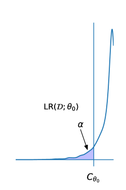
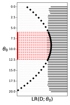
Figure 2: Neyman construction of confidence sets by inverting hypothesis tests. Left: For each $\theta_{0}\in\Theta$, we find the critical value $C_{\theta_{0}}$ that rejects the null hypothesis $H_{0,\theta_{0}}$ at level $\alpha$; that is, $C_{\theta_{0}}$ is the $\alpha$-quantile of the distribution of the test statistic under the null (a likelihood ratio $\text{LR}(\mathcal{D};\theta_{0})$ in this case). Right: The horizontal solid lines represent acceptance regions for each $\theta_{0}\in\Theta$. Suppose we observe data $D$. The confidence set for $\theta$ (red vertical solid line) consists of all $\theta_{0}$-values for which the observed test statistic $\text{LR}(D;\theta_{0})$ (black curve) falls in the acceptance region.

3 Likelihood-Free Frequentist Inference via Odds Estimation

In the typical LFI setting, we cannot directly evaluate the likelihood ratio $\text{LR}({\mathcal{D}};\Theta_{0})$ or even the likelihood $\mathcal{L}({\mathcal{D}};\theta)$. In this work, we describe a version of LF2I that is based on odds estimation. We assume that we have access to (i) a forward simulator $F_{\theta}$ to draw observable data, (ii) a reference distribution $G$ that does not depend on $\theta$, with larger support than $F_{\theta}$ for all $\theta\in\Theta$, and (iii) a probabilistic classifier to discriminates samples from $F_{\theta}$ and $G$.

3.1 Estimating an Odds Function across the Parameter Space

We start by generating a labeled sample ${\mathcal{T}}=\{(\theta_{i},{\mathbf{X}}_{i},Y_{i})\}_{i=1}^{B}$ to compare data from $F_{\theta}$ with data from the reference distribution $G$. Here, $\theta\sim\pi_{\Theta}$ (a proposal distribution over $\Theta$), the “label” $Y\sim\text{Ber}(p)$, ${\mathbf{X}}|(\theta,Y=1)\sim F_{\theta}$ and ${\mathbf{X}}|(\theta,Y=0)\sim G$. We then define the odds at $\theta$ and fixed ${\mathbf{x}}$ as

$${\mathbb{O}}({\mathbf{x}};\theta):=\frac{{\mathbb{P}}(Y=1|\theta,{\mathbf{x}})}{{\mathbb{P}}(Y=0|\theta,{\mathbf{x}})}.$$ (7)

One way of interpreting ${\mathbb{O}}({\mathbf{x}};\theta)$ is to regard it as a measure of the chance that ${\mathbf{x}}$ was generated from $F_{\theta}$ rather than from $G$. That is, a large odds ${\mathbb{O}}({\mathbf{x}};\theta)$ reflects the fact that it is plausible that ${\mathbf{x}}$ was generated from $F_{\theta}$ (instead of $G$). We call $G$ a “reference distribution” as we are comparing $F_{\theta}$ for different $\theta$ with this distribution. Equation 7 is equivalent to the likelihood $p({\mathbf{x}}|\theta)$ up to a normalization constant, as shown in [26, Proposition 3.1]. The odds function ${\mathbb{O}}({\mathbf{X}};\theta)$ with $\theta\in\Theta$ as a parameter can be estimated with a probabilistic classifier, such as a neural network with a softmax layer, suitable for the data at hand. Algorithm 3 in Appendix A summarizes our procedure for simulating a labeled sample ${\mathcal{T}}$. For all experiments in this paper, we use p=1/2 and $G=F_{\mathbf{X}}$, where $F_{\mathbf{X}}$ is the (empirical) marginal distribution of $F_{\theta}$ with respect to $\pi_{\Theta}$.

3.2 Test Statistics based on Odds Function

For testing $H_{0,\Theta_{0}}:\theta\in\Theta_{0}$ versus all alternatives $H_{1,\Theta_{0}}:\theta\notin\Theta_{0}$, we consider two test statistics: ACORE and BFF. Both statistics are based on $\mathbb{O}({\mathbf{X}};\theta)$, but whereas ACORE eliminates the parameter $\theta$ by maximization, BFF averages over the parameter space.

3.2.1 ACORE by Maximization

The ACORE statistic [26] for testing Equation 3 is given by

$$\Lambda({\mathcal{D}};\Theta_{0}) :=\log\frac{\sup_{\theta\in\Theta_{0}}\prod_{i=1}^{n}\mathbb{O}({\mathbf{X}}_{i};\theta)}{\sup_{\theta\in\Theta}\prod_{i=1}^{n}\mathbb{O}({\mathbf{X}}_{i};\theta)}$$

$$=\ \sup_{\theta_{0}\in\Theta_{0}}\inf_{\theta_{1}\in\Theta}\sum_{i=1}^{n}\log\left(\mathbb{OR}({\mathbf{X}}_{i};\theta_{0},\theta_{1})\right),$$ (8)

where the odds ratio

$$\mathbb{OR}({\mathbf{x}};\theta_{0},\theta_{1}):=\frac{\mathbb{O}({\mathbf{x}};\theta_{0})}{\mathbb{O}({\mathbf{x}};\theta_{1})}$$ (9)

at $\theta_{0},\theta_{1}\in\Theta$ measures the plausibility that a fixed ${\mathbf{x}}$ was generated from $\theta_{0}$ rather than $\theta_{1}$. We use $\widehat{\Lambda}({\mathcal{D}};\Theta_{0})$ to denote the ACORE statistic based on ${\mathcal{T}}$ and estimated odds $\widehat{\mathbb{O}}({\mathbf{X}};\theta_{0})$. When $\widehat{\mathbb{O}}({\mathbf{X}};\theta_{0})$ is well-estimated for every $\theta$ and ${\mathbf{X}}$, $\widehat{\Lambda}({\mathcal{D}};\Theta_{0})$ is the same as the $\text{LR}({\mathcal{D}};\Theta_{0})$ in Equation 5 [26, Proposition 3.1].

3.2.2 BFF by Averaging

Because the ACORE statistics in Equation 8 involves taking the supremum (or infimum) over $\Theta$, it may not be practical in high dimensions. Hence, in this work, we propose an alternative statistic for testing (3) based on averaged odds:

$$\tau({\mathcal{D}};\Theta_{0}):=\frac{\int_{\Theta_{0}}\prod_{i=1}^{n}\mathbb{O}({\mathbf{X}}_{i};\theta_{0})d\pi_{0}(\theta)}{\int_{\Theta_{0}^{c}}\prod_{i=1}^{n}\mathbb{O}({\mathbf{X}}_{i};\theta)d\pi_{1}(\theta)},$$ (10)

where $\pi_{0}$ and $\pi_{1}$ are the restrictions of the proposal distribution $\pi$ to the parameter regions $\Theta_{0}$ and $\Theta_{0}^{c}$, respectively. Let $\widehat{\tau}({\mathcal{D}};\Theta_{0})$ denote estimates based on ${\mathcal{T}}$ and $\widehat{\mathbb{O}}(\theta_{0};{\mathbf{x}})$. If the probabilities learned by the classifier are well estimated, then the estimated averaged odds statistic $\widehat{\tau}({\mathcal{D}};\Theta_{0})$ is exactly the Bayes factor:

Proposition 1 (Fisher consistency)

Assume that, for every $\theta\in\Theta$, $G$ dominates $\nu$. If $\ \widehat{{\mathbb{P}}}(Y=1|\theta,{\mathbf{x}})={\mathbb{P}}(Y=1|\theta,{\mathbf{x}})$ for every $\theta$ and ${\mathbf{x}}$, then $\widehat{\tau}({\mathcal{D}};\Theta_{0})$ is the Bayes factor $\text{BF}({\mathcal{D}};\Theta_{0})$.

In this paper, we are using the Bayes factor as a frequentist test statistic. Hence, our term Bayes Frequentist Factor (BFF) statistic for $\tau$ and $\widehat{\tau}$.

3.3 Fast Construction of Neyman Confidence Sets

Instead of a costly MC or bootstrap hypothesis test of $H_{0}:\theta=\theta_{0}$ at each $\theta_{0}$ on a fine grid (see, e.g., [62] and [88]), we draw only one sample $\mathcal{T}^{\prime}$ of size $B^{\prime}$. We then estimate either the critical value $C_{\theta_{0}}$ via quantile regression (Section 3.3.1), or the p-value $p(D;\theta_{0})$ via probabilistic classification (Section 3.3.2), for all $\theta_{0}\in\Theta$ simultaneously. In Supplementary Material G, we propose a practical strategy to choose the number of simulations $B^{\prime}$ and the learning algorithm.

3.3.1 The Critical Value via Quantile Regression

Algorithm 1 describes how to use quantile regression (e.g., [68, 54]) to estimate the critical value $C_{\theta_{0}}$ for a level-$\alpha$ test of (3) as a function of $\theta_{0}\in\Theta$. To test a composite null hypothesis $H_{0}:\theta\in\Theta_{0}$ versus $H_{1}:\theta\in\Theta_{1}$, we use the cutoff $\widehat{C}_{\Theta_{0}}:=\inf_{\theta\in\Theta_{0}}\widehat{C}_{\theta}$. Although we originally proposed the calibration procedure for ACORE, the same scheme leads to a valid test (control of type I error as the number of simulations $B^{\prime}\rightarrow\infty$) for any test statistic $\lambda$ (Theorem 9). Remarkably, this holds even if the test statistic is not well estimated. Note that in practice, we observe that the number of simulations $B^{\prime}$ needed to achieve correct coverage is usually much lower relative to $B$, the number of simulations needed to estimate the test statistic. In addition, Algorithm 1 does not require observed data $D$ and is hence amortized, meaning that once both the test statistic and the critical values are estimated, we can compute confidence sets for an arbitrary number of observations.

Algorithm 1 Estimate critical values $C_{\theta_{0}}$ for a level-$\alpha$ test of $H_{0,\theta_{0}}:\theta=\theta_{0}$ vs. $H_{1,\theta_{0}}:\theta\neq\theta_{0}$ for all $\theta_{0}\in\Theta$ simultaneously

Input: simulator $F_{\theta}$; number of simulations $B^{\prime}$; $\pi_{\Theta}$ (fixed proposal distribution over the parameter space); test statistic $\lambda$; quantile regression estimator; level $\alpha\in(0,1)$ Output: estimated critical values $\widehat{C}_{\theta_{0}}$ for all $\theta_{0}\in\Theta$

1:Set ${\mathcal{T}}^{\prime}\leftarrow\emptyset$

2:for i in $\{1,\ldots,B^{\prime}\}$ do

3:    Draw parameter $\theta_{i}\sim\pi_{\Theta}$

4:    Draw sample ${\mathbf{X}}_{i,1},\ldots,{\mathbf{X}}_{i,n}\stackrel{{\scriptstyle iid}}{{\sim}}F_{\theta_{i}}$

5:    Compute test statistic $\lambda_{i}\leftarrow\lambda(({\mathbf{X}}_{i,1},\ldots,{\mathbf{X}}_{i,n});\theta_{i})$

6:    ${\mathcal{T}}^{\prime}\leftarrow{\mathcal{T}}^{\prime}\cup\{(\theta_{i},\lambda_{i})\}$

7:end for

8:Use ${\mathcal{T}}^{\prime}$ to learn the conditional quantile function $\widehat{C}_{\theta}:=\widehat{F}_{\lambda|\theta}^{-1}(\alpha|\theta)$ via quantile regression of $\lambda$ on $\theta$

9:return $\widehat{C}_{\theta_{0}}$

3.3.2 The P-Value via Probabilistic Classification

If the data $D$ are observed beforehand, then given any test statistic $\lambda$ we can alternatively compute p-values for each hypothesis $H_{0,\theta_{0}}:\theta=\theta_{0}$, that is,

$$p(D;\theta_{0}):={\mathbb{P}}_{\mathcal{D}|\theta_{0}}\left(\lambda({\mathcal{D}};\theta_{0})<\lambda(D;\theta_{0})\right).$$ (11)

The p-value $p(D;\theta_{0})$ can be used to test hypothesis and create confidence sets for any desired level $\alpha$. As detailed in Algorithm 5, we can estimate it simultaneously for all $\theta\in\Theta$ by drawing a training sample ${\mathcal{T}}^{\prime}=\{(Z_{1},\theta_{1}),\ldots,$ $(Z_{B^{\prime}},\theta_{B^{\prime}})\}$ and using the random variable $Z:={\mathbb{I}}\left(\lambda({\mathcal{D}};\theta)<\lambda(D;\theta)\right)$ as a label for each $\theta$. To test the composite null hypothesis $H_{0}:\theta\in\Theta_{0}$ versus $H_{1}:\theta\in\Theta_{1}$, we use

$$\widehat{p}(D;\Theta_{0}):=\sup_{\theta\in\Theta_{0}}\widehat{p}(D;\theta).$$

Note that there is a key computational difference between estimating p-values versus estimating critical values. The p-value is a function of both $\theta$ and the observed sample $D$ itself. As a result, Algorithm 5 has to be repeated for each observed $D$, making the computation of p-values non-amortized.

3.3.3 Amortized Confidence Sets

Finally, we construct an approximate confidence region for $\theta$ by taking the set

$$\widehat{R}(D)=\left\{\theta\in\Theta\ \middle|\lambda(D;\theta)\geq\widehat{C}_{\theta}\right\},$$ (12)

or, alternatively,

$$\widehat{R}(D)=\left\{\theta\in\Theta\,\middle|\,\widehat{p}(D;\theta)>\alpha\right\}.$$ (13)

See Algorithm 6 in Appendix C for details. As shown in [26, Theorem 3.3], the random set $\widehat{R}({\mathcal{D}})$ has nominal $(1-\alpha)$ coverage as $B^{\prime}\rightarrow\infty$ regardless of the observed sample size $n$. As noted in Section 3.3.1, the confidence set in Equation 12 is fully amortized, meaning that once we have $\lambda({\mathcal{D}};\theta)$ and $\widehat{C}_{\theta}$ as a function of $\theta\in\Theta$, we can perform inference on new data without retraining.

3.4 Diagnostics: Checking Coverage across the Parameter Space

Algorithm 2 Estimate empirical coverage $\mathbb{P}_{\mathcal{D}|\theta}(\theta\in\widehat{R}({\mathcal{D}}))$, for all $\theta\in\Theta$.

Input: simulator $F_{\theta}$; number of simulations $B^{\prime\prime}$; $\pi_{\Theta}$ (fixed proposal distribution over parameter space); test statistic $\lambda$; level $\alpha$; critical values $\widehat{C}_{\theta}$; probabilistic classifier Output: estimated coverage $\widehat{\mathbb{P}}_{\mathcal{D}|\theta}(\theta\in\widehat{R}({\mathcal{D}}))$ for all $\theta\in\Theta$

1:Set ${\mathcal{T}}^{\prime\prime}\leftarrow\emptyset$

2:for i in $\{1,\ldots,B^{{}^{\prime\prime}}\}$ do

3:    Draw parameter $\theta_{i}\sim\pi_{\Theta}$

4:    Draw sample ${\mathcal{D}}_{i}:=\{{\mathbf{X}}_{i,1},\ldots,{\mathbf{X}}_{i,n}\}\stackrel{{\scriptstyle iid}}{{\sim}}F_{\theta_{i}}$

5:    Compute test statistic $\lambda_{i}\leftarrow\lambda({\mathcal{D}}_{i};\theta_{i})$

6:    Compute indicator variable $W_{i}\leftarrow{\mathbb{I}}\left(\lambda_{i}\geq\widehat{C}_{\theta_{i}}\right)$

7:    ${\mathcal{T}}^{\prime\prime}\leftarrow{\mathcal{T}}^{\prime\prime}\cup\{(\theta_{i},W_{i})\}$

8:end for

9: Use ${\mathcal{T}}^{\prime\prime}$ to learn $\widehat{\mathbb{P}}_{\mathcal{D}|\theta^{\prime}}(\theta^{\prime}\in\widehat{R}({\mathcal{D}}))$ across $\Theta$ by regressing $W$ on $\theta$

10:return $\widehat{\mathbb{P}}_{\mathcal{D}|\theta}(\theta\in\widehat{R}({\mathcal{D}}))$

The LF2I framework has a separate module (“Diagnostics” in Figure 1) for evaluating “local” goodness-of-fit in different regions of the parameter space $\Theta$. This estimates the coverage probability ${\mathbb{P}}_{{\mathcal{D}}|\theta}(\theta\in\widehat{R}({\mathcal{D}}))$ of confidence sets $\widehat{R}({\mathcal{D}})$ across the parameter space via probabilistic classification. As detailed in Algorithm 2, we first generate a set of size $B^{\prime\prime}$ from the simulator: $\mathcal{T}^{\prime\prime}=\{(\theta_{1},\mathcal{D}_{1}),\ldots,(\theta_{B^{\prime\prime}},\mathcal{D}_{B^{\prime\prime}})\}$. Then, for each sample $\mathcal{D}_{i}$, we check whether or not the test statistic $\lambda_{i}$ is larger than the estimated critical value $\widehat{C}_{\theta_{i}}$ (the output from Algorithm 1). This is equivalent to computing a binary variable $W_{i}$ for whether or not the “true” value $\theta_{i}$ falls within the confidence set $\widehat{R}({\mathcal{D}}_{i})$ (Equation 12). Recall that the computations of the test statistic and the critical value are amortized, meaning that we do not retrain algorithms to estimate these two quantities. The final step is to estimate empirical coverage as a function of $\theta$ by using $W$ as a label for each $\theta$. This estimation requires a new fit, but after training the probabilistic classifier, we can evaluate the estimated coverage anywhere in parameter space $\Theta$.

This diagnostic procedure locates regions in parameter space where estimated confidence sets might under- or over-cover; see Figures 3, 4 and 6 for examples. Note that standard goodness-of-fit techniques for conditional densities [16, 9, 84, 79] only check for marginal coverage over $\Theta$.

4 Theoretical Guarantees

We now prove consistency of the critical value and p-value estimation methods (Algorithms 1 and 5, respectively) and provide theoretical guarantees for the power of BFF. We refer the reader to Appendix D for a proof for finite $\Theta$ that the power of ACORE converges to the power of LRT as $B$ grows (Theorem 7).

In this section, ${\mathbb{P}}_{{\mathcal{D}},{\mathcal{T}}^{\prime}|\theta}$ denotes the probability integrated over both ${\mathcal{D}}\sim F_{\theta}$ and ${\mathcal{T}}^{\prime}$, whereas ${\mathbb{P}}_{{\mathcal{D}}|\theta}$ denotes integration over ${\mathcal{D}}\sim F_{\theta}$ only. For notational ease, we do not explicitly state again (inside the parentheses of the same expression) that we condition on $\theta$.

4.1 Critical Value Estimation

We start by showing that our procedure for choosing critical values leads to valid hypothesis tests (that is, tests that control the type I error probability), as long as the number of simulations $B^{\prime}$ in Algorithm 1 is sufficiently large. We assume that the null hypothesis is simple, that is, $\Theta_{0}=\{\theta_{0}\}$ — which is the relevant setting for the Neyman construction of confidence sets in the absence of nuisance parameters. See Theorem 9 in Appendix E for results for composite null hypotheses.

We assume that the quantile regression estimator described in Section 3.3.1 is consistent in the following sense:

Assumption 1 (Uniform consistency)

Let $F(\cdot|\theta)$ be the cumulative distribution function of the test statistic $\lambda(\mathcal{D};\theta_{0})$ conditional on $\theta$, where ${\mathcal{D}}\sim F_{\theta}$. Let $\widehat{F}_{B^{\prime}}(\cdot|\theta)$ be the estimated conditional distribution function, implied by a quantile regression with a sample $\mathcal{T}^{{}^{\prime}}$ of $B^{\prime}$ simulations ${\mathcal{D}}\sim F_{\theta}$. Assume that the quantile regression estimator is such that

$$\sup_{\lambda\in\mathbb{R}}|\widehat{F}_{B^{\prime}}(\lambda|\theta_{0})-F(\lambda|\theta_{0})|\xrightarrow[B^{\prime}\longrightarrow\infty]{\enskip{\mathbb{P}}\enskip}0.$$

Assumption 1 holds, for instance, for quantile regression forests [68].

Next, we show that Algorithm 1 yields a valid hypothesis test as $B^{\prime}\rightarrow\infty$.

Theorem 1

Let $C_{B^{\prime}}\in\mathbb{R}$ be the critical value of the test based on an absolutely continuous statistic $\lambda(\mathcal{D};\theta_{0})$ chosen according to Algorithm 1 for a fixed $\alpha\in(0,1)$. If the quantile estimator satisfies Assumption 1, then, for every $\theta_{0},\theta\in\Theta$,

$${\mathbb{P}}_{\mathcal{D}|\theta_{0},C_{B^{\prime}}}(\lambda(\mathcal{D};\theta_{0})\leq C_{B^{\prime}})\xrightarrow[B^{\prime}\longrightarrow\infty]{\enskip a.s.\enskip}\alpha,$$

where ${\mathbb{P}}_{\mathcal{D}|\theta_{0},C_{B^{\prime}}}$ denotes the probability integrated over $\mathcal{D}\sim F_{\theta_{0}}$ and conditional on the random variable $C_{B^{\prime}}$.

If the convergence rate of the quantile regression estimator is known (Assumption 2), Theorem 2 provides a finite-$B^{\prime}$ guarantee on how far the type I error of the test will be from the nominal level.

Assumption 2 (Convergence rate of the quantile regression estimator)

Using the notation of Assumption 1, assume that the quantile regression estimator is such that

$$\sup_{\lambda\in\mathbb{R}}|\widehat{F}_{B^{\prime}}(\lambda|\theta_{0})-F(\lambda|\theta_{0})|=O_{P}\left(\left(\frac{1}{B^{\prime}}\right)^{r}\right)$$

for some $r>0$.

Theorem 2

With the notation and assumptions of Theorem 1, and if Assumption 2 also holds, then,

$$|{\mathbb{P}}_{\mathcal{D}|\theta_{0},C_{B^{\prime}}}(\lambda(\mathcal{D};\theta_{0})\leq C_{B^{\prime}})-\alpha|=O_{P}\left(\left(\frac{1}{B^{\prime}}\right)^{r}\right).$$

4.2 P-Value Estimation

Next we show that the p-value estimation method described in Section 3.3.2 is consistent. The results shown here apply to any test statistic $\lambda$. That is, these results are not restricted to BFF.

We assume consistency in the sup norm of the regression method used to estimate the p-values:

Assumption 3 (Uniform consistency)

The regression estimator used in Equation 11 is such that

$$\sup_{\theta}|\widehat{\mathbb{E}}_{B^{\prime}}[Z|\theta]-{\mathbb{E}}[Z|\theta]|\xrightarrow[B^{\prime}\longrightarrow\infty]{\enskip\text{a.s.}\enskip}0.$$

Examples of estimators that satisfy Assumption 3 include [7, 41, 57, 38].

The next theorem shows that the p-values obtained according to Algorithm 5 converge to the true p-values. Moreover, the power of the tests obtained using the estimated p-values converges to the power one would obtain if the true p-values could be computed.

Theorem 3

Under Assumption 3 and if $p({\mathcal{D}};\Theta_{0})$ is an absolutely continuous random variable then, for every $\theta\in\Theta$,

$$\widehat{p}(D;\Theta_{0})\xrightarrow[B^{\prime}\longrightarrow\infty]{\enskip\text{a.s.}\enskip}p(D;\Theta_{0})$$

and

$${\mathbb{P}}_{{\mathcal{D}},{\mathcal{T}}^{\prime}|\theta}(\widehat{p}({\mathcal{D}};\Theta_{0})\leq\alpha)\xrightarrow{B^{\prime}\longrightarrow\infty}{\mathbb{P}}_{{\mathcal{D}}|\theta}(p({\mathcal{D}};\Theta_{0})\leq\alpha).$$

The next corollary shows that as $B^{\prime}\longrightarrow\infty$, the tests obtained using the p-values from Algorithm 5 have size $\alpha$.

Corollary 1

Under Assumption 3 and if $F_{\theta}$ is continuous for every $\theta\in\Theta$ and $p({\mathcal{D}};\Theta_{0})$ is an absolutely continuous random variable, then

$$\sup_{\theta\in\Theta_{0}}{\mathbb{P}}_{{\mathcal{D}},{\mathcal{T}}^{\prime}|\theta}(\widehat{p}({\mathcal{D}};\Theta_{0})\leq\alpha)\xrightarrow{B^{\prime}\longrightarrow\infty}\alpha.$$

Under stronger assumptions about the regression method, it is also possible to derive rates of convergence for the estimated p-values.

Assumption 4 (Convergence rate of the regression estimator)

The regression estimator is such that

$$\sup_{\theta}|\widehat{\mathbb{E}}[Z|\theta]-{\mathbb{E}}[Z|\theta]|=O_{P}\left(\left(\frac{1}{B^{\prime}}\right)^{r}\right).$$

for some $r>0$.

Examples of regression estimators that satisfy Assumption 4 can be found in [83, 41, 29, 94].

Theorem 4

Under Assumption 4,

$$|p(D;\Theta_{0})-\widehat{p}(D;\Theta_{0})|=O_{P}\left(\left(\frac{1}{B^{\prime}}\right)^{r}\right).$$

4.3 Power of BFF

In this section, we provide convergence rates for BFF and show that its power relates to the integrated squared error

$$\mathcal{L}(\widehat{\mathbb{O}},\mathbb{O}):=\int\left(\widehat{\mathbb{O}}({\mathbf{x}};\theta)-\mathbb{O}({\mathbf{x}};\theta)\right)^{2}dG({\mathbf{x}})d\pi(\theta),$$ (14)

which measures how well we are able to estimate the odds function.

We assume that we are testing a simple hypothesis $H_{0,\theta_{0}}:\theta=\theta_{0},$ where $\theta_{0}$ is fixed, and that $G({\mathbf{x}})$ is the marginal distribution of ${\color[rgb]{0,0,0}X\sim\ }F_{\theta}({\mathbf{x}})$ with respect to $\pi(\theta)$. We also assume that ${\mathbf{x}}$ contains all observations; that is, $\mathbf{X}={\mathcal{D}}$. In this case, the denominator of the average odds is

$$\begin{split}\int_{\Theta}\mathbb{O}({\mathbf{x}},\theta)d\pi(\theta)&=\int_{\Theta_{1}}\frac{p\cdot p({\mathbf{x}}|\theta)}{(1-p)g({\mathbf{x}})}d\pi(\theta)\\ &=\frac{p}{1-p}\int_{\Theta}\frac{p({\mathbf{x}}|\theta)}{\int_{\Theta}p({\mathbf{x}}|\theta)d\pi(\theta)}d\pi(\theta)=\frac{p}{1-p},\end{split}$$

where $g$ is the density of $G$ with respect to $\nu$ and therefore there is no need to estimate the denominator in Equation 10.

We also assume that the odds and estimated odds are both bounded away from zero and infinity:

Assumption 5 (Bounded odds and estimated odds)

There exists $0<m,M<\infty$ such that for every $\theta\in\Theta$ and ${\mathbf{x}}\in\mathcal{X}$, $m\leq\mathbb{O}({\mathbf{x}};\theta),\widehat{\mathbb{O}}({\mathbf{x}};\theta)\leq M$.

Finally, we assume that the CDF of the power function of the test based on the BFF statistic $\tau$ in Equation 10 is smooth in a Lipschitz sense:

Assumption 6 (Smooth power function)

For every $\theta_{0}\in\Theta$, the cumulative distribution function of $\tau({\mathcal{D}};\theta_{0})$, $F_{\tau}$, is Lipschitz with constant $C_{L}$, i.e., for every $x_{1},x_{2}\in\mathbb{R}$, $|F_{\tau}(x_{1})-F_{\tau}(x_{2})|\leq C_{L}|x_{1}-x_{2}|$.

With these assumptions, we can relate the odds loss with the probability that the outcome of BFF is different from the outcome of the test based on the Bayes factor:

Theorem 5

For fixed $c\in\mathbb{R}$, let $\phi_{\tau;\theta_{0}}({\mathcal{D}})={\mathbb{I}}\left(\tau({\mathcal{D}};\theta_{0})<c\right)$ and $\phi_{\widehat{\tau}_{B};\theta_{0}}({\mathcal{D}})={\mathbb{I}}\left(\widehat{\tau}_{B}({\mathcal{D}};\theta_{0})<c\right)$ be the testing procedures for testing $H_{0,\theta_{0}}:\theta=\theta_{0}$ based on $\tau$ and $\widehat{\tau}_{B}$, respectively. Under Assumptions 5-6, for every $0<\epsilon<1$ and $\theta\in\Theta$,

$$\int{\mathbb{P}}_{\mathcal{D}|\theta,T}(\phi_{\tau;\theta_{0}}({\mathcal{D}})\neq\phi_{\widehat{\tau}_{B};\theta_{0}}({\mathcal{D}}))d\pi(\theta_{0})\leq\frac{2MC_{L}\cdot\sqrt{L(\widehat{\mathbb{O}},\mathbb{O})}}{\epsilon}+\epsilon,$$

where $T$ denotes the realized training sample $\mathcal{T}$ and ${\mathbb{P}}_{\mathcal{D}|\theta,T}$ is the probability measure integrated over the observable data ${\mathcal{D}}\sim F_{\theta}$, but conditional on the train sample used to create the test statistic.

Theorem 5 demonstrates that, on average (over $\theta_{0}\sim\pi$), the probability that hypothesis tests based on the BFF statistic versus the Bayes factor lead to different conclusions is bounded by the integrated odds loss. This result is valuable because the integrated odds loss is easy to estimate in practice, and hence provides us with a practically useful metric. For instance, the integrated odds loss can serve as a natural criterion for selecting the “best” statistical model out of a set of candidate models with different classifiers, for tuning model hyperparameters, and for evaluating model fit.

Next, we provide rates of convergence of the test based on BFF to the test based on the Bayes factor. We assume that the chosen probabilistic classifier has the following rate of convergence:

Assumption 7 (Convergence rate of the probabilistic classifier)

The probabilistic classifier trained with ${\mathcal{T}}$, $\widehat{\mathbb{P}}(Y=1|{\mathbf{x}},\theta)$ is such that

$${\mathbb{E}}_{{\mathcal{T}}}\left[\int\left(\widehat{\mathbb{P}}(Y=1|{\mathbf{x}},\theta)-{\mathbb{P}}(Y=1|{\mathbf{x}},\theta)\right)^{2}dH({\mathbf{x}},\theta)\right]=O\left(B^{-\kappa/(\kappa+d)}\right),$$

for some $\kappa>0$ and $d>0$, where $H({\mathbf{x}},\theta)$ is a measure over $\mathcal{X}\times\Theta$.

Typically, $\kappa$ relates to the smoothness of ${\mathbb{P}}$, while $d$ relates to the number of covariates of the classifier — in our case, the number of parameters plus the number of features. In Supplementary Material H, we provide some examples where Assumption 7 holds.

We also assume that the density of the product measure $G\times\pi$ is bounded away from infinity.

Assumption 8 (Bounded density)

$H({\mathbf{x}},\theta)$ dominates $H^{\prime}:=G\times\pi$, and the density of $H^{\prime}$ with respect to $H$, denoted by $h^{\prime}$, is such that there exists $\gamma>0$ with $h^{\prime}({\mathbf{x}},\theta)<\gamma,\ \forall{\mathbf{x}}\in\mathcal{X},\theta\in\Theta$.

If the probabilistic classifier has the convergence rate given by Assumption 7, then the average probability that hypothesis tests based on the BFF statistic versus the Bayes factor goes to zero has the rate given by the following theorem.

Theorem 6

Let $\phi_{\tau;\theta_{0}}({\mathcal{D}})$ and $\phi_{\widehat{\tau}_{B};\theta_{0}}({\mathcal{D}})$ be as in Theorem 5. Under Assumptions 5-8, there exists $K^{\prime}>0$ such that, for any $\theta\in\Theta$,

$$\int{\mathbb{P}}_{\mathcal{D},{\mathcal{T}}|\theta}(\phi_{\tau;\theta_{0}}({\mathcal{D}})\neq\phi_{\widehat{\tau}_{B};\theta_{0}}({\mathcal{D}}))d\pi(\theta_{0})\leq K^{\prime}B^{-\kappa/(4(\kappa+d))}.$$

Corollary 2

Under Assumptions 5-8, there exists $K^{\prime}>0$ such that, for any $\theta\in\Theta$,

$$\int{\mathbb{P}}_{\mathcal{D},{\mathcal{T}}|\theta}(\phi_{\widehat{\tau}_{B};\theta_{0}}({\mathcal{D}})=1)d\theta_{0}\geq\int{\mathbb{P}}_{\mathcal{D},{\mathcal{T}}|\theta}(\phi_{\tau;\theta_{0}}({\mathcal{D}})=1)d\theta_{0}-K^{\prime}B^{-\kappa/(4(\kappa+d))}.$$

Corollary 2 tells us that the average power of the BFF test is close to the average power of the exact Bayes factor test. This result also implies that BFF converges to the most powerful test in the Neyman-Person setting, where the Bayes factor test is equivalent to the LRT.

5 Handling Nuisance Parameters

In most applications, we only have a small number of parameters that are of primary interest. The other parameters in the model are usually referred to as nuisance parameters. In this setting, we decompose the parameter space as $\Theta=\Phi\times\Psi$, where $\Phi$ contains the parameters of interest, and $\Psi$ contains nuisance parameters. Our goal is to construct a confidence set for $\phi\in\Phi$. To guarantee frequentist coverage by Neyman’s inversion technique, however, one needs to test null hypotheses of the form $H_{0,\phi_{0}}:\phi=\phi_{0}$ by comparing the test statistics to the cutoffs $\widehat{C}_{\phi_{0}}:=\inf_{\psi\in\Psi}\widehat{C}_{(\phi_{0},\psi)}$ (Section 3.3.1). That is, one needs to control the type I error at each $\phi_{0}$ for all possible values of the nuisance parameters. Computing such infimum can be numerically unwieldy, especially if the number of nuisance parameters is large [87, 96]. Below we propose approximate schemes for handling nuisance parameters:

In ACORE, we use a hybrid resampling or “likelihood profiling” method [14, 34, 80] to circumvent unwieldy numerical calculations as well as to reduce computational cost. For each $\phi$ (on a fine grid over $\Phi$), we first compute the “profiled” value

$$\widehat{\psi}_{\phi}=\arg\max_{\psi\in\Psi}\prod_{i=1}^{n}\widehat{\mathbb{O}}\left({\mathbf{x}}^{\rm obs}_{i};(\phi,\psi)\right),$$

which (because of the odds estimation) is an approximation of the maximum likelihood estimate of $\psi$ at the parameter value $\phi$ for observed data $D$. By definition, the estimated ACORE test statistic for the hypothesis $H_{0,\phi_{0}}:\phi=\phi_{0}$ is exactly given by $\widehat{\Lambda}(\mathcal{D};\phi_{0})=\widehat{\Lambda}(\mathcal{D};(\phi_{0},\widehat{\psi}_{\phi_{0}}))$. However, rather than comparing this statistic to $\widehat{C}_{\phi_{0}}$, we use the hybrid cutoff

$$\widehat{C}^{\prime}_{\phi_{0}}:=\widehat{F}^{-1}_{\widehat{\Lambda}\left({\mathcal{D}};\phi_{0}\right)\big{|}\left(\phi_{0},\widehat{\psi}_{\phi_{0}}\right)}\left(\alpha\,\middle|\,\phi_{0},\widehat{\psi}_{\phi_{0}}\right),$$ (15)

where $\widehat{F}^{-1}$ is obtained via a quantile regression as in Algorithm 1, but using a training sample ${\mathcal{T}}^{\prime}$ generated at fixed $\widehat{\psi}_{\phi_{0}}$ (that is, we run Algorithm 1 with the proposal distribution $\pi^{\prime}((\phi,\psi))\propto\pi(\phi)\times\delta_{\widehat{\psi}_{\phi}}(\psi),$ where $\delta_{\widehat{\psi}_{\phi}}(\psi)$ is a point mass distribution at $\widehat{\psi}_{\phi}$). Alternatively, one can compute the p-value

$$\widehat{p}(D;\phi_{0}):=\widehat{\mathbb{E}}\left[{\mathbb{I}}\left(\widehat{\Lambda}\left({\mathcal{D}};\phi_{0}\right)<\widehat{\Lambda}\left(D;\phi_{0}\right)\right)\,\middle|\,\phi_{0},\widehat{\psi}_{\phi_{0}}\right]$$ (16)

via probabilistic classification as in Algorithm 5, but with ${\mathcal{T}}^{\prime}$ simulated at fixed $\widehat{\psi}_{\phi_{0}}$ (that is, we run Algorithm 5 with the proposal distribution $\pi^{\prime}((\phi,\psi))\propto\pi(\phi)\times\delta_{\widehat{\psi}_{\phi}}(\psi)$. Hybrid methods do not always control $\alpha$, but they are often a good approximation that lead to robust results [1, 76]. We refer to ACORE approaches based on Equation 15 or Equation 16 as “h-ACORE” approaches.

In contrast to ACORE, the BFF test statistic averages (rather than maximizes) over nuisance parameters. Hence, instead of adopting a hybrid resampling scheme to handle nuisance parameters, we approximate p-values and critical values, in what we refer to as “h-BFF”, by using the marginal model of the data ${\mathcal{D}}$ at a parameter of interest $\phi$:

$$\mathcal{\widetilde{L}}(D;\phi)=\int_{\psi\in\Psi}\mathcal{L}(D;\theta)\,d\pi(\psi).$$

We implement such a scheme by first drawing the train sample $\mathcal{T}^{{}^{\prime}}$ from the entire parameter space $\Theta=\Phi\times\Psi$, and then applying quantile regression (or probabilistic classification) using $\phi$ only.

Algorithm 7 details our construction of ACORE and BFF confidence sets when calibrating critical values under the presence of nuisance parameter (construction via p-value estimation is analogous). In Section 6.2, we demonstrate how our diagnostics branch can shed light on whether or not the final results have adequate frequentist coverage.

6 Experiments

We analyze the empirical performance of the LF2I framework under different problem settings: unknown null distribution of the test statistic (Section 6.1); nuisance parameters (Section 6.2); intractable likelihood and high-dimensional data (Section 6.3).

We use the cross-entropy loss (Eq. F) when estimating the odds function in Equation 7 and the empirical coverage probability as in Section 3.4 via probabilistic classification. Moreover, we use the pinball loss [54] when estimating critical values as in Section 3.3.1 via quantile regression.

6.1 Gaussian Mixture Model: Unknown Null Distribution

A common practice in LFI is to first estimate the likelihood and then assume that the LR statistic is approximately $\chi^{2}$ distributed according to Wilks’ theorem [31]. However, in settings with small sample sizes or irregular statistical models, such approaches may lead to confidence sets with incorrect coverage; it is often difficult to identify exactly when that happens, and then know how to recalibrate the confidence sets. (See [4] for a discussion of all conditions needed for Wilks’ theorem to apply, which are often not realized in practice.)

The Gaussian mixture model (GMM) is a classical example where the LR statistic is known but its null distribution is unknown in finite samples. Indeed, the development of valid statistical methods for GMM is an active area of research [78, 66, 25, 12, 90]. Here we consider a one-dimensional Normal mixture with unknown mean but known unit variance:

$$X\sim 0.5N(\theta,1)+0.5N(-\theta,1),$$

where the parameter of interest $\theta\in\Theta=[0,5]$. We analyze three different approaches for estimating the critical value $C_{\theta_{0}}$ of a level-$\alpha$ LRT of the hypothesis test $H_{0,\theta_{0}}:\theta=\theta_{0}$, for different $\theta_{0}\in\Theta$:

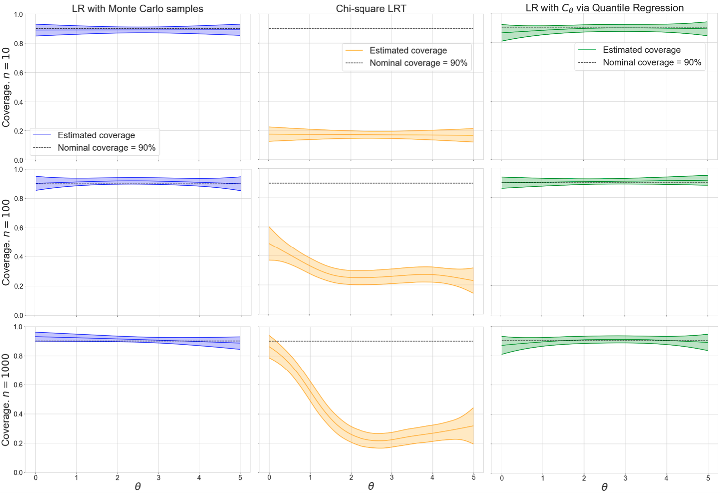
Figure 3: GMM with unknown null distribution. Each panel shows the estimated coverage across the parameter space of 90% confidence sets for $\theta$. Rows represent experiments with different observed sample sizes: $n=10,100,1000$ (top, center, bottom). Columns represent three different approaches. Left: “LR with Monte Carlo samples” achieves nominal coverage everywhere but is computationally expensive, especially in higher dimensions. Center: “Chi-square LRT” clearly under-covers, i.e. confidence sets are not valid even for large $n$, other than at $\theta=0$ where the mixture collapses to one Gaussian. Right: “LR with $C_{\theta_{0}}$ via quantile regression” returns finite-sample confidence sets with the nominal coverage of $90\%$ for all values of $\theta$, but using a total of 1000 simulations, instead of a MC sample of 1000 simulations at each grid point.

• “LR with Monte Carlo samples”, where we draw 1000 simulations at each point $\theta_{0}$ on a fine grid over $\Theta$ and take $C_{\theta_{0}}$ to be the $1-\alpha$ quantile of the distribution of the LR statistic, computed using the MC samples at each fixed $\theta_{0}$. This approach is often just referred to as MC hypothesis testing.

• “Chi-square LRT”, where we assume that $-2\text{LR}({\mathcal{D}};\theta_{0})\sim\chi^{2}_{1}$, and hence take $-2C_{\theta_{0}}$ to be the same as the upper $\alpha$ quantile of a $\chi^{2}_{1}$ distribution.

• “LR with $C_{\theta_{0}}$ via quantile regression”, where we estimate $C_{\theta_{0}}$ via quantile regression (Algorithm 1) based on a total of $B^{\prime}=1000$ simulations of size $n$ sampled uniformly on $\Theta$.

We then construct confidence sets by inverting the hypothesis tests, and finally assess their conditional coverage with the diagnostic branch of the LF2I framework (Algorithm 2 with $B^{\prime\prime}=1000$).

Figure 3 shows LF2I diagnostics for the three different approaches when the data sample size is $n=10,100,1000$. Confidence sets from “Chi-square LRT” are clearly not valid at any $n$, which shows that Wilks’ theorem does not apply in this setting. The only exception arises when $n$ is large enough and $\theta$ approaches 0, in which case the mixture reduces to a unimodal Gaussian whose LR statistic has a known limiting distribution (see bottom center panel of Figure 3). On the other hand, “LR with $C_{\theta_{0}}$ via quantile regression” returns valid finite-sample confidence sets with conditional coverage equivalent to “LR with Monte Carlo samples”. A key difference between the LF2I and MC methods is that the LF2I results are based on 1000 samples in total, whereas the MC results are based on 1000 MC samples at each $\theta_{0}$ on a grid. The latter approach quickly becomes intractable in higher parameter dimensions and larger scales.

Supplementary Material I gives details on the specific quantile regressor (for Algorithm 1) and probabilistic classifier (for Algorithm 2) used in Figure 3, and presents extensions of the above experiments to confidence sets via p-value estimation and asymmetric mixtures.

6.2 Poisson Counting Experiment: Nuisance Parameters and Diagnostics

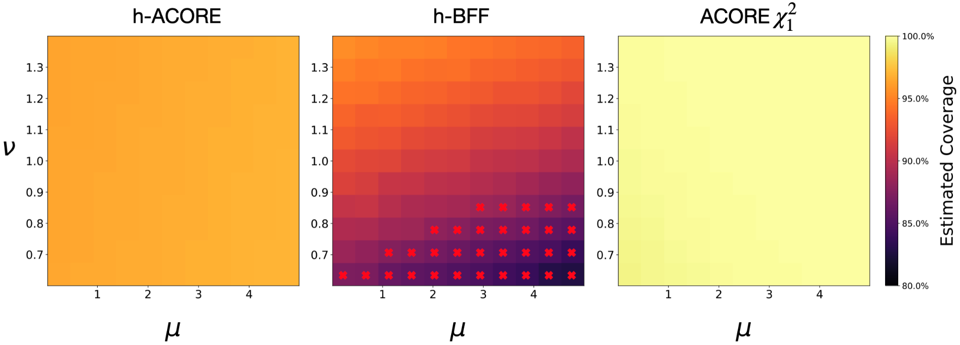
Figure 4: Poisson counting experiment with nuisance parameters. The diagnostics branch provides guidance as to which LFI approach to use for the problem at hand by pinpointing regions of the parameter space $\Theta$ where inference is unreliable. The panels show empirical coverage as a function of both $\mu$, the parameter of interest, and $\nu$, the nuisance parameter. Nominal coverage is $90\%$. Left: h-ACORE, which uses profiled likelihoods, is overly conservative in terms of actual coverage ($\approx 96\%$) across $\Theta$. Center: h-BFF, which marginalizes over $\nu$, under-covers in several regions (red crosses). Right: ACORE $\chi_{1}^{2}$, which uses cutoffs from the chi-square distribution, has almost no constraining power, yielding empirical coverage close to $100\%$ everywhere.

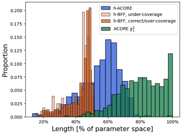
Figure 5: Constraining power. The histograms show the length of the confidence sets constructed for the counting experiment, as a percentage of the total length of the parameter of interest space. ACORE $\chi_{1}^{2}$ and h-ACORE are overly conservative and yield the widest intervals. h-BFF provides tighter confidence sets, but their size is not reliable when the method under-covers. LF2I diagnostics can identify those parameter regions (red crosses in Figure 4).

Hybrid methods, which maximize or marginalize over nuisance parameters, do not always control the type I error of statistical tests. For small sample sizes, there is no theorem as to whether profiling or marginalization of nuisance parameters will give better frequentist coverage for the parameter of interest [18, Section 12.5.1]. In addition, most practitioners consider a thorough check of frequentist coverage to be impractical [18, Section 13]. In this example, we apply the hybrid schemes from Section 5 to a high-energy physics (HEP) counting experiment [61, 21, 20, 19, 42] with nuisance parameters , which is a simplified version of a real particle physics experiment where the true likelihood function is not known. We illustrate how our diagnostics can guide the analyst and provide insight into which method to choose for the problem at hand.

Consider a “Poisson counting experiment” where particle collision events are counted under the presence of both an uncertain background process and a (new) signal process. The goal is to estimate the signal strength. To avoid identifiability issues, the background rate is estimated separately by counting the number of events in a control region where the signal is believed to be absent. Hence, the observable data $\mathbf{X}=(N_{b},N_{s})$ contain two measurements, where $N_{b}\sim{\rm Pois}(\nu\tau b)$ is the number of events in the control region, and $N_{s}\sim{\rm Pois}(\nu b+\mu s)$ is the number of events in the signal region. Our parameter of interest is the signal strength $\mu$, whereas the scaling factor for the background $\nu$ is a nuisance parameter. The hyper-parameters $s$ and $b$ indicate the nominally expected counts from signal and backgrounds, and $\tau$ describes the relationship in measurement time between the two processes. We treat the three hyper-parameters as known with values $s=15$, $b=70$, $\tau=1$, respectively. The hyper-parameters move the model away from the Gaussian limiting regime and make the relationship between data and parameters more complicated [42].

We compare the hybrid methods h-ACORE and h-BFF with ACORE $\chi^{2}_{1}$ (which uses cutoffs from the chi-square distribution). We learn the odds using a QDA classifier with $B=100{,}000$ and estimate critical values for the hybrid methods via quantile gradient boosted trees with $B^{\prime}=10{,}000$. We evaluate the different methods on a separate set of size $B^{\prime\prime}=1{,}000$ by estimating coverage and measuring the length of confidence sets for each of the simulated samples.

Figure 4 shows the estimated coverage as a function of both $\mu$ and $\nu$. Confidence sets are considered to be valid when they achieve the nominal coverage level regardless of the true value of both the parameter of interest and the nuisance parameters. Both h-ACORE and ACORE $\chi_{1}^{2}$ are overly conservative across the whole parameter space, while h-BFF under-covers in regions of high signal strength and low background. These results are consistent with the length of the corresponding confidence sets shown in Figure 5: h-ACORE and ACORE $\chi_{1}^{2}$ are overly conservative, with the former being almost uninformative for the majority of evaluation samples. On the other side, while h-BFF seems to provide tighter parameter constraints, their length can be trusted only in regions where the method has coverage at least equal to the nominal level. Our LF2I diagnostic branch can pinpoint the regions of the parameter space where inference is reliable or not.

6.3 Muon Energy Estimation: Intractable Likelihood and High-Dimensional Data

We now showcase LF2I on a high-energy physics application with intractable likelihood and very high-dimensional data. The goal is to estimate the energy of muons using a high-granularity calorimeter in a particle collider experiment. Muons are subatomic particles that have proven to be excellent probes of new physical phenomena: their detection and measurement has enabled several crucial discoveries in the last few decades, including the discovery of the Higgs boson [5, 43, 15, 2, 11]. Traditionally, the energy of a muon is determined from the curvature of its trajectory in a magnetic field, but curvature-based measurements have proven to be insufficiently precise at high energies. Recently, muon energy measurements based on their radiative losses in a dense, finely segmented calorimeter (Figure 6, left) have been shown to be a feasible alternative [53, 30].

In this application, the dimensionality of one data point ${\mathbf{x}}$ (a 3D image) is of the order of $\approx 50{,}000$ and the observed sample size is $n=1$ (as each unique data point is the output of one experiment with a specific parameter of interest $\theta$). In total, we have available $886{,}716$ 3D “image” inputs $\mathbf{x}$ with corresponding scalar muon energies $\theta$. The data are obtained by accurately mimicking particle showers with GEANT4 [3], a high-fidelity simulator that has been calibrated for decades and is trusted to incorporate all the dynamics of the Standard Model of particle physics. The data are available at [52].

The scientific goal of this experiment is to quantify whether a high-granularity calorimeter would better constrain the energy of a muon (that is, lead to smaller confidence sets) than, for example, a detector that only measures the total energy of the incoming particle. To answer this question, we consider nested versions of the same energy measurement, where the inputs to our algorithms are of increasing dimensionality: (i) a 1D input which is equal to the sum over all the cells of the calorimeter (for each muon with deposited energy $E>0.1$ GeV); (ii) 28 custom features extracted from the spatial and energy information of the calorimeter cells (see [53]); and (iii) the full calorimeter measurement, $\mathbf{x}\in\mathbb{R}^{51{,}200}$. We then construct LF2I confidence sets for each data point using BFF. On the full calorimeter data, we learn the odds function through a convolutional neural network classifier derived from the regressor proposed in [53], and estimate critical values via quantile gradient boosted trees. For the 1D and 28D data sets, we instead learn odds through a gradient boosting classifier. In both cases, we use approximately $83\%$ of the data to learn the odds function ($B=738{,}930$) and $14\%$ to estimate critical values ($B^{\prime}=123{,}155$). For comparison, we also include results from SMC-ABC [82], a popular LFI algorithm from the Approximate Bayesian Computation literature. To provide a fair assessment of the results, SMC-ABC uses all the simulations that LF2I exploits separately (i.e., $B+B^{\prime}=862{,}085$). The remaining data points ($B^{\prime\prime}=24{,}631$) are used for validation and diagnostics of both methods.

Figure 6 (center) shows that LF2I with the BFF test statistic achieves the nominal level of coverage ($68.3\%$) regardless of the data set used. This is consistent with Theorem 1: as long as the quantile regression is well estimated, LF2I confidence sets are guaranteed to be valid at the nominal $(1-\alpha)$ level regardless of how well the test statistic is estimated. On the other hand, SMC-ABC is overly conservative with credible intervals that strongly over-cover across the whole parameter space. As to constraining power (interval length), Figure 6 (right) shows that SMC-ABC credible intervals are significantly wider than LF2I confidence sets for both the 1D and 28D data sets (running SMC-ABC on the $51{,}200$-dimensional full calorimeter data was computationally infeasible, and we were not able to report the results). Finally, note how the amount of information in the data directly influences the size of LF2I confidence sets: going from the 1D data set to the full calorimeter leads to noticeably smaller confidence intervals, and hence higher constraining power.

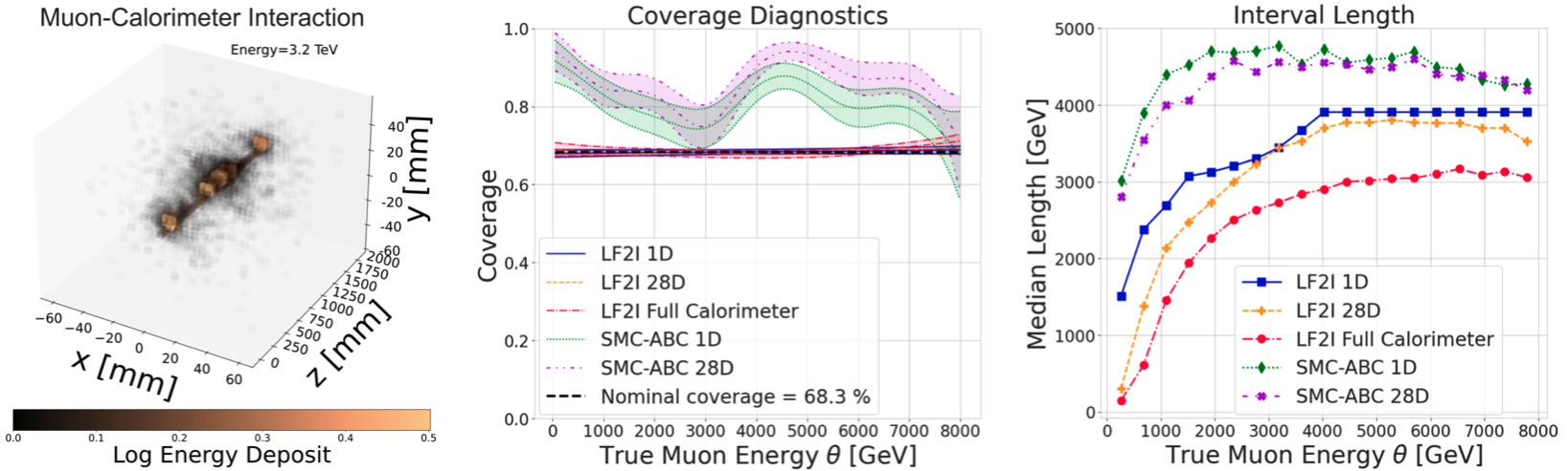
Figure 6: Muon energy estimation. LF2I guarantees nominal coverage and yields smaller confidence intervals relative to SMC-ABC. Left: Data point example of a muon with incoming energy $\theta\approx 3.2$ TeV entering a calorimeter with $32\times 32\times 50$ cells. Center: LF2I (blue, orange, red in the right two panels) achieves coverage at the nominal level (68.3%), whereas SMC-ABC (green and purple) is consistently over-covering across the parameter space. Right: Median lengths of constructed intervals. While being extremely computationally intensive, SMC-ABC has also the least constraining power regardless of the data set used. SMC-ABC on the full calorimeter data is not reported as it was computationally infeasible to run.

Remark on Validity and Computational Cost

SMC-ABC does not have the right coverage, because the goal of ABC is to construct Bayesian credible regions and not valid confidence sets; see, e.g., [45] for other examples of SMC-ABC under- or over-covering. Furthermore, note that (i) LF2I is amortized: once training is done, confidence sets can be efficiently computed on an arbitrary number of observations without having to retrain the algorithms; and (ii) there is no need for a prior dimension reduction of the data (that is, we can directly input the three-dimensional image). Specifically, LF2I required approximately 10 and 5 CPU minutes on an AMD’s EPYC 7763 machine to train the odds classifier and the quantile regressor respectively, and less than a second to obtain confidence intervals all at once for all observations (in this example, unique $24{,}631$ “test” muons) regardless of their dimensionality. In contrast, SMC-ABC required approximately 1 CPU hour for each observation even for the lower-dimensional 1D and 28D datasets.

7 Conclusions and Discussion

Validity

Our proposed LF2I methodology leads to frequentist confidence sets and hypothesis tests with finite-sample guarantees (when there are no nuisance parameters). Any existing or new test statistic – that is, not only estimates of the LR or BF statistics – can be plugged into our framework to create tests that control type I error. The implicit assumption is that the null distribution of the test statistic varies smoothly in parameter space. If that condition holds, then we can efficiently leverage quantile regression methods to construct valid confidence sets by a Neyman inversion of simple hypothesis tests, without having to rely on asymptotic results. In settings where the likelihood can be evaluated, our framework leads to more powerful tests and smaller confidence sets than universal inference, but at the cost of having to simulate data from the likelihood.

Nuisance parameters and diagnostics

For small sample sizes, there is no theorem to tell us whether profiling or marginalization of nuisance parameters will give better frequentist coverage for the parameter of interest [18, Section 12.5.1]. It is generally believed that hybrid resampling methods return approximately valid confidence sets, but that a rigorous check of validity is infeasible when the true solution is not known. Our diagnostic branch presents practical tools for assessing empirical coverage across the entire parameter space (including nuisance parameters). After seeing the results, one can decide which method is most appropriate for the application at hand. For example, in the Poisson counting experiment of Section 6.2, LF2I diagnostics revealed that h-BFF (which averages the estimated odds over nuisance parameters) returned smaller confidence intervals, but at the cost of under-covering in some regions of the parameter space.

Power

Statistical power is the hardest property to achieve in practice in LFI. This is the area where we foresee that most statistical and computational advances will take place. As shown theoretically in Theorem 5 and empirically in Supplementary Material J, the power (or size) of LF2I confidence sets depends not only on the theoretical properties of the (exact) test statistics, but is also influenced by how precisely we are able to estimate it. In the case of ACORE and BFF, the latter can be divided in (i) how well we are able to estimate the likelihood or odds function (a statistical estimation error), and (ii) how accurate are the integration or maximization procedures we use (a purely numerical error); see Supplementary Material G for a more precise breakdown of the sources of error in LF2I confidence sets, particularly for ACORE and BFF. Machine learning offers exciting possibilities on both fronts. For example, with regards to (i), [10] offers compelling evidence that one can can dramatically improve estimates of the likelihood $p({\mathbf{x}}|\theta)$ for $\theta\in\Theta$, or the likelihood ratio $p({\mathbf{x}}|\theta_{1},\theta_{2})$ for $\theta_{1},\theta_{2}\in\Theta$, by a “mining gold” approach that extracts additional information from the simulator about the latent process. Future work could incorporate such an approach into the LF2I framework, with the calibration and diagnostic branches as separate modules.

Other test statistics

Our work presents also another new direction for LF2I: So far frequentist LFI methods have been estimating either likelihoods or likelihood ratios, and then often relying on asymptotic properties of the LR statistic. We note that there are settings where it may be easier to either estimate the posterior $p(\theta|{\mathbf{x}})$ rather than the likelihood $p({\mathbf{x}}|\theta)$ , or alternatively to obtain point estimates for parameters directly via predictions algorithms. Because the LF2I framework is agnostic to which algorithms we use to construct the test statistic itself, we can potentially leverage methods that estimate the conditional mean $\mathbb{E}[\theta|{\mathbf{x}}]$ and variance $\mathbb{V}[\theta|{\mathbf{x}}]$ to construct frequentist confidence sets and hypothesis tests for $\theta$ with finite-sample guarantees. For example, [65] uses $T=\frac{(\mathbb{E}[\theta|{\mathbf{x}}]-\theta_{0})^{2}}{\mathbb{V}[\theta|{\mathbf{x}}]}$, which in some scenarios corresponds to the Wald statistic for testing $H_{0,\theta_{0}}:\theta=\theta_{0}$ against $H_{1,\theta_{0}}:\theta\neq\theta_{0}$ [89], as an attractive alternative to get LF2I confidence sets from prediction algorithms and posterior estimators.

See Appendices A-F for proofs and details on the algorithms, and refer to the separate Supplementary Material file for additional experiments and results referenced in the main text.

[Acknowledgments] The authors would like to thank Mikael Kuusela, Rafael Stern and Larry Wasserman for helpful discussions. We are also indebted to Tommaso Dorigo, Jan Kieseler and Giles C. Strong for providing the muon energy data and the neural network architecture used for the studies described in Section 6.3.

Appendix A Estimating Odds

Algorithm 3 provides details on how to create the training sample ${\mathcal{T}}$ for estimating odds. Out of the total number of simulations $B$, a proportion $p$ is generated by the stochastic forward simulator $F_{\theta}$ at different parameter values $\theta$, while the rest is sampled from a reference distribution $G$. Note that $G$ can be any distribution that dominates $F_{\theta}$. If $G$ is the marginal distribution $F_{\mathbf{x}}$ and the observed sample size is $n=1$, then the denominator of the BFF statistic is exactly equal to one, allowing us to bypass the calculation of the denominator. Algorithm 4 shows how to sample from the marginal distribution $F_{\mathbf{x}}$. In practice, if the data is pre-simulated, one can sample from the (empirical) marginal using permutations to break the relationship between $\theta$ and ${\mathbf{X}}$ for ${\mathbf{X}}\sim G=F_{\mathbf{x}}$.

Algorithm 3 Generate a labeled sample of size $B$ for estimating odds

Input: simulator $F_{\theta}$; reference distribution $G$; proposal distribution $\pi_{\Theta}$ over parameter space; number of simulations $B$; parameter $p$ of Bernoulli distribution Output: labeled training sample ${\mathcal{T}}$

1:Set ${\mathcal{T}}\leftarrow\emptyset$

2:for $i$ in $\{1,...,B\}$ do

3:    Draw parameter value $\theta_{i}\sim\pi_{\Theta}$

4:    Draw $Y_{i}\sim{\rm Ber}(p)$

5:    if $Y_{i}==1$ then

6:         Draw sample ${\mathbf{X}}_{i}\sim F_{\theta_{i}}$

7:    else

8:         Draw sample ${\mathbf{X}}_{i}\sim G$

9:    end if

10:    ${\mathcal{T}}\leftarrow{\mathcal{T}}\cup\left(\theta_{i},{\mathbf{X}}_{i},Y_{i}\right)$

11:end for

12:return ${\mathcal{T}}=\{\theta_{i},{\mathbf{X}}_{i},Y_{i}\}_{i=1}^{B}$

Algorithm 4 Sample from the marginal distribution $G=F_{{\mathbf{X}}}$

Input: simulator $F_{\theta}$; proposal distribution $\pi_{\Theta}$ over parameter space

Output: sample ${\mathbf{X}}_{i}$ from the marginal distribution $F_{{\mathbf{X}}}$

1:Draw parameter value $\theta_{i}\sim\pi_{\Theta}$

2:Draw sample ${\mathbf{X}}_{i}\sim F_{\theta_{i}}$

3:return ${\mathbf{X}}_{i}$

Appendix B Estimating P-Values

Algorithm 5 Estimate p-values $p(D;\theta_{0})$ given observed data $D$ for a level-$\alpha$ test of $H_{0,\theta_{0}}:\theta=\theta_{0}$ vs. $H_{1,\theta_{0}}:\theta\neq\theta_{0}$, for all $\theta_{0}\in\Theta$ simultaneously.

Input: observed data $D$; simulator $F_{\theta}$; number of simulations $B^{\prime}$; $\pi_{\Theta}$ (fixed proposal distribution over the parameter space $\Theta$); test statistic $\lambda$; probabilistic classifier Output: estimated p-value $\widehat{p}(D;\theta)$ for all $\theta=\theta_{0}\in\Theta$

1: Set ${\mathcal{T}}^{\prime}\leftarrow\emptyset$

2:for i in $\{1,\ldots,B^{\prime}\}$ do

3:    Draw parameter $\theta_{i}\sim\pi_{\Theta}$

4:    Draw sample ${\mathbf{X}}_{i,1},\ldots,{\mathbf{X}}_{i,n}\stackrel{{\scriptstyle iid}}{{\sim}}F_{\theta_{i}}$

5:    Compute test statistic $\lambda_{i}\leftarrow\lambda(({\mathbf{X}}_{i,1},\ldots,{\mathbf{X}}_{i,n});\theta_{i})$

6:    Compute indicator $Z_{i}\leftarrow{\mathbb{I}}\left(\lambda_{i}<\lambda(D;\theta_{i})\right)$

7:    ${\mathcal{T}}^{\prime}\leftarrow{\mathcal{T}}^{\prime}\cup\{(\theta_{i},Z_{i})\}$

8:end for

9:Use ${\mathcal{T}}^{\prime}$ to learn the p-value function $\widehat{p}(D;\theta)$ using $Z$ as the label for each $\theta$

10:return $\widehat{p}(D;\theta_{0})$

Appendix C Constructing Confidence Sets

Algorithm 6 details the construction of LF2I confidence sets with ACORE and BFF as defined in Section 3 (the algorithm based on p-value estimation is analogous). Algorithm 7 details the construction of the (hybrid) ACORE and BFF confidence sets defined in Section 5 for the general setting with nuisance parameters. Note that the first chunk on estimating the odds and the last chunk with Neyman inversion are the same for ACORE and BFF. Furthermore, the test statistics are the same whether or not there are nuisance parameters.

Algorithm 6 Construct $(1-\alpha)$ confidence set for $\theta$ (no nuisance parameters)

Input: simulator $F_{\theta}$; proposal distribution $\pi$ over $\Theta$; parameter $p$ of Bernoulli; number of simulations $B$ (test statistic); number of simulations $B^{\prime}$ (critical values); probabilistic classifier; observations $D=\{{\mathbf{x}}_{i}^{\text{obs}}\}_{i=1}^{n}$; level $\alpha\in(0,1)$; size of evaluation grid over parameter space $n_{\rm grid}$; test statistic $\lambda$ (ACORE or BFF)

Output: $\theta$ evaluation points in confidence set $\widehat{R}(D)$

1:// Estimate odds

2:Generate labeled sample ${\mathcal{T}}$ according to Algorithm 3

3:Apply probabilistic classifier to ${\mathcal{T}}$ to learn $\widehat{{\mathbb{P}}}(Y=1|\theta,{\mathbf{X}}),$ for all $\theta\in\Theta$ and ${\mathbf{X}}\in\mathcal{X}$

4:Let the estimated odds $\widehat{\mathbb{O}}({\mathbf{X}};\theta)\leftarrow\frac{\widehat{{\mathbb{P}}}(Y=1|\theta,{\mathbf{X}})}{\widehat{{\mathbb{P}}}(Y=0|\theta,{\mathbf{X}})}$

5:

6:// Compute cut-offs for ACORE or BFF

7:if $\lambda$ == ACORE then

8:    Let $\lambda({\mathcal{D}};\theta)\leftarrow\widehat{\Lambda}({\mathcal{D}};\theta)$ be the ACORE statistic (Equation 8) with estimated odds

9:else if test_stat == BFF then

10:    Let $\lambda({\mathcal{D}};\theta)\leftarrow\widehat{\tau}({\mathcal{D}};\theta)$ be the BFF statistic (Equation 10) with estimated odds

11:end if

12:Learn critical values $\widehat{C}_{\theta}$ according to Algorithm 1

13:

14:// Confidence sets for $\theta$ via Neyman inversion

15:Initialize confidence set $\widehat{R}(D)\leftarrow\emptyset$

16:Let ${\rm L}_{\Theta}$ be a lattice over $\Theta$ with $n_{\rm grid}$ elements

17:for $\theta_{0}\in{\rm L}_{\Theta}$ do

18:    if  $\lambda(D;\theta_{0})\geq\widehat{C}_{\theta_{0}}$  then

19:         $\widehat{R}(D)\leftarrow\widehat{R}(D)\cup\{\theta_{0}\}$

20:    end if

21:end for

22:return confidence set $\widehat{R}(D)$

Algorithm 7 Construct confidence set for $\phi$ with (approximate) coverage $1-\alpha$ under the presence of nuisance parameters

Input: simulator $F_{\theta}$; proposal distribution $\pi$ over $\Theta=\Phi\times\Psi$; parameter $p$ of Bernoulli; number of simulations $B$ (test statistic); number of simulations $B^{\prime}$ (critical values); probabilistic classifier; observations $D=\{{\mathbf{x}}_{i}^{\text{obs}}\}_{i=1}^{n}$; level $\alpha\in(0,1)$; size of evaluation grid over parameter space, $n_{\rm grid}$; test statistic $\lambda$ (ACORE or BFF)

Output: $\phi$ evaluation points in confidence set $\widehat{R}(D)$

1:// Estimate odds

2:Generate labeled sample ${\mathcal{T}}$ according to Algorithm 3

3:Apply probabilistic classifier to ${\mathcal{T}}$ to learn $\widehat{{\mathbb{P}}}(Y=1|\theta,{\mathbf{X}}),$ $\forall\text{ }\theta=(\phi,\psi)\in\Theta,{\mathbf{X}}\in\mathcal{X}$

4:Let the estimated odds $\widehat{\mathbb{O}}({\mathbf{X}};\theta)\leftarrow\frac{\widehat{{\mathbb{P}}}(Y=1|\theta,{\mathbf{X}})}{\widehat{{\mathbb{P}}}(Y=0|\theta,{\mathbf{X}})}$

5:

6:// Compute (hybrid) critical values for h-ACORE or h-BFF

7:if $\lambda$ == ACORE then

8:    Let $\widehat{\psi}_{\phi}\leftarrow\arg\max_{\psi\in\Psi}\prod_{i=1}^{n}\widehat{\mathbb{O}}({\mathbf{x}}_{i}^{\rm obs};(\phi,\psi))$ for every $\phi$

9:    Let $\lambda({\mathcal{D}};\phi)\leftarrow\widehat{\Lambda}\left({\mathcal{D}};(\phi,\widehat{\psi}_{\phi})\right)$ be ACORE (Equation 8) with estimated odds

10:    Generate $\mathcal{T}^{\prime}$ as in Algorithm 1 using the proposal $\pi^{\prime}((\phi,\psi))\propto\pi(\phi)\times\delta_{\widehat{\psi}_{\phi}}(\psi)$

11:    Learn $\widehat{C}_{\phi}=\widehat{F}^{-1}_{\lambda\left({\mathcal{D}};\phi\right)\big{|}\left(\phi,\widehat{\psi}_{\phi}\right)}(\alpha)$ for every $\phi$ as in Algorithm 1 using ${\mathcal{T}}^{\prime}$

12:else if $\lambda$ == BFF then

13:    Let $\pi_{\Psi}(\psi)$ be the restriction of proposal distribution $\pi$ over $\Psi$

14:    Let $\lambda({\mathcal{D}};\phi)\leftarrow\widehat{\tau}({\mathcal{D}};\phi)$ be the BFF statistic (Equation 10) with estimated odds

15:    Learn $\widehat{C}_{\phi}=\widehat{F}^{-1}_{\lambda\left({\mathcal{D}};\phi\right)\big{|}\left(\phi\right)}(\alpha)$ for every $\phi$ (no $\psi$) as in Algorithm 1

16:end if

17:

18:// Confidence sets for $\phi$ via Neyman inversion

19:Initialize confidence set $\widehat{R}(D)\leftarrow\emptyset$

20:Let ${\rm L}_{\Phi}$ be a lattice over $\Phi$ with $n_{\rm grid}$ elements

21:for $\phi_{0}\in{\rm L}_{\Phi}$ do

22:    if  $\lambda(D;\phi_{0})\geq\widehat{C}_{\phi_{0}}$  then

23:         $\widehat{R}(D)\leftarrow\widehat{R}(D)\cup\{\phi_{0}\}$

24:    end if

25:end for

26:return confidence set $\widehat{R}(D)$

Appendix D Theoretical Guarantees of power for ACORE with Calibrated Critical Values

Next, we show , for finite $\Theta$, that as long as the probabilistic classifier is consistent and the critical values are well estimated (which holds for large $B^{\prime}$ according to Theorem 9), the power of the ACORE test converges to the power of the LRT as $B$ grows.

Theorem 7

For each $C\in\mathbb{R}$, let $\widehat{\phi}_{B,C}(\mathcal{D})$ be the test based on the ACORE statistic $\widehat{\Lambda}_{B}$ with critical value $C$ for number of simulations $B$ in Algorithm 3. Moreover, let $\phi_{C}(\mathcal{D})$ be the likelihood ratio test with critical value $C$. If, for every $\theta\in\Theta$, the probabilistic classifier is such that

$$\widehat{{\mathbb{P}}}(Y=1|\theta,{\mathbf{X}})\xrightarrow[B\longrightarrow\infty]{\enskip{\mathbb{P}}\enskip}{\mathbb{P}}(Y=1|\theta,{\mathbf{X}}),$$

where $|\Theta|<\infty$, and $\widehat{C}_{B}$ is chosen such that $\widehat{C}_{B}\xrightarrow[B\longrightarrow\infty]{\enskip\mbox{Dist}\enskip}C$ for a given $C\in\mathbb{R}$, then, for every $\theta\in\Theta$,

$${\mathbb{P}}_{\mathcal{D},{\mathcal{T}}|\theta}\left(\widehat{\phi}_{B,\widehat{C}_{B}}(\mathcal{D})=1\right)\xrightarrow[B\longrightarrow\infty]{}{\mathbb{P}}_{\mathcal{D}|\theta}\left(\phi_{C}(\mathcal{D})=1\right).$$

Proof D.1.

Because $\widehat{{\mathbb{P}}}(Y=1|\theta,{\mathbf{X}})\xrightarrow[B\longrightarrow\infty]{\enskip{\mathbb{P}}\enskip}{\mathbb{P}}(Y=1|\theta,{\mathbf{X}})$, it follows directly from the properties of convergence in probability that for every $\theta_{0},\theta_{1}\in\Theta$

$$\sum_{i=1}^{n}\log \left(\widehat{\mathbb{OR}}({\mathbf{X}}_{i}^{\text{obs}};\theta_{0},\theta_{1})\right)\xrightarrow[B\longrightarrow\infty]{\enskip{\mathbb{P}}\enskip}\sum_{i=1}^{n}\log\left(\mathbb{OR}({\mathbf{X}}_{i}^{\text{obs}};\theta_{0},\theta_{1})\right).$$

The continuous mapping theorem implies that

$$\widehat{\Lambda}_{B}({\mathcal{D}};\Theta_{0})\xrightarrow[B\longrightarrow\infty]{\enskip{\mathbb{P}}\enskip}\sup_{\theta_{0}\in\Theta_{0}}\inf_{\theta_{1}\in\Theta}\sum_{i=1}^{n}\log\left(\mathbb{OR}({\mathbf{X}}_{i}^{\text{obs}};\theta_{0},\theta_{1})\right),$$

and therefore $\widehat{\Lambda}_{B}({\mathcal{D}};\Theta_{0})$ converges in distribution to $\sup_{\theta_{0}\in\Theta_{0}}\inf_{\theta_{1}\in\Theta}\sum_{i=1}^{n}\log\left(\mathbb{OR}({\mathbf{X}}_{i}^{\text{obs}};\theta_{0},\theta_{1})\right)$. Now, from Slutsky’s theorem,

$$\widehat{\Lambda}_{B}({\mathcal{D}};\Theta_{0})-\widehat{C}_{B}\xrightarrow[B\longrightarrow\infty]{\enskip\mbox{Dist}\enskip}\sup_{\theta_{0}\in\Theta_{0}}\inf_{\theta_{1}\in\Theta}\sum_{i=1}^{n}\log\left(\mathbb{OR}({\mathbf{X}}_{i}^{\text{obs}};\theta_{0},\theta_{1})\right)-C.$$

It follows that

$${\mathbb{P}}_{\mathcal{D},{\mathcal{T}}|\theta}\left(\widehat{\phi}_{B,\widehat{C}_{B}}(\mathcal{D})=1\right)={\mathbb{P}}_{\mathcal{D},{\mathcal{T}}|\theta}\left(\widehat{\Lambda}_{B}({\mathcal{D}};\Theta_{0})-\widehat{C}_{B}\leq 0\right)$$

$$\xrightarrow[B\longrightarrow\infty]{}{\mathbb{P}}_{\mathcal{D}|\theta}\Big{(}\sup_{\theta_{0}\in\Theta_{0}}\inf_{\theta_{1}\in\Theta}\sum_{i=1}^{n}\log\left(\mathbb{OR}({\mathbf{X}}_{i}^{\text{obs}};\theta_{0},\theta_{1})\right)-C\leq 0\Big{)}$$

$$={\mathbb{P}}_{\mathcal{D}|\theta}\left(\phi_{C}(\mathcal{D})=1\right),$$

where the last equality follows from Proposition 1.

Appendix E Additional Proofs

Proof E.1 (Proof of Proposition 1).

Because $\nu$ dominates $F_{\theta}$, $G$ also dominates $F_{\theta}$. Let $f({\mathbf{x}}|\theta)$ be the density of $F_{\theta}$ with respect to $G$. By Bayes rule,

$${\mathbb{O}}({\mathbf{x}};\theta):=\frac{{\mathbb{P}}(Y=1|\theta,{\mathbf{x}})}{{\mathbb{P}}(Y=0|\theta,{\mathbf{x}})}=\frac{f({\mathbf{x}}|\theta)p}{(1-p)}.$$

If $\ \widehat{{\mathbb{P}}}(Y=1|\theta,{\mathbf{x}})={\mathbb{P}}(Y=1|\theta,{\mathbf{x}})$, then $\widehat{\mathbb{O}}({\mathbf{x}};\theta_{0})=\mathbb{O}({\mathbf{x}};\theta_{0})$. Therefore,

$$\widehat{\tau}({\mathcal{D}};\Theta_{0}):= \frac{\int_{\Theta_{0}}\prod_{i=1}^{n}\widehat{\mathbb{O}}({\mathbf{X}}_{i}^{\text{obs}};\theta)d\pi_{0}(\theta)}{\int_{\Theta_{1}}\prod_{i=1}^{n}\widehat{\mathbb{O}}({\mathbf{X}}_{i}^{\text{obs}};\theta)d\pi_{1}(\theta)}$$

$$= \frac{\int_{\Theta_{0}}\prod_{i=1}^{n}\mathbb{O}({\mathbf{X}}_{i}^{\text{obs}};\theta)d\pi_{0}(\theta)}{\int_{\Theta_{1}}\prod_{i=1}^{n}\mathbb{O}({\mathbf{X}}_{i}^{\text{obs}};\theta)d\pi_{1}(\theta)}$$

$$= \frac{\int_{\Theta_{0}}\prod_{i=1}^{n}\frac{f({\mathbf{X}}_{i}^{\text{obs}}|\theta)p}{(1-p)}d\pi_{0}(\theta)}{\int_{\Theta_{1}}\prod_{i=1}^{n}\frac{f({\mathbf{X}}_{i}^{\text{obs}}|\theta)p}{(1-p)}d\pi_{1}(\theta)}$$

$$= \frac{\int_{\Theta_{0}}\prod_{i=1}^{n}f({\mathbf{X}}_{i}^{\text{obs}}|\theta)d\pi_{0}(\theta)}{\int_{\Theta_{1}}\prod_{i=1}^{n}f({\mathbf{X}}_{i}^{\text{obs}}|\theta)d\pi_{1}(\theta)}$$

Moreover, the chain rule implies that $f({\mathbf{x}}|\theta)=p({\mathbf{x}}|\theta)h({\mathbf{x}})$, where $h({\mathbf{x}}):=\frac{d\nu}{dG}({\mathbf{x}})$. It follows that

$$\widehat{\tau}({\mathcal{D}};\Theta_{0})= \frac{\int_{\Theta_{0}}\prod_{i=1}^{n}f({\mathbf{X}}_{i}^{\text{obs}}|\theta)d\pi_{0}(\theta)}{\int_{\Theta_{1}}\prod_{i=1}^{n}f({\mathbf{X}}_{i}^{\text{obs}}|\theta)d\pi_{1}(\theta)}$$

$$=\frac{\int_{\Theta_{0}}\prod_{i=1}^{n}p({\mathbf{X}}_{i}^{\text{obs}}|\theta)h({\mathbf{X}}_{i}^{\text{obs}})d\pi_{0}(\theta)}{\int_{\Theta_{1}}\prod_{i=1}^{n}p({\mathbf{X}}_{i}^{\text{obs}}|\theta)h({\mathbf{X}}_{i}^{\text{obs}})d\pi_{1}(\theta)}$$

$$=\frac{\int_{\Theta_{0}}\prod_{i=1}^{n}p({\mathbf{X}}_{i}^{\text{obs}}|\theta)d\pi_{0}(\theta)}{\int_{\Theta_{1}}\prod_{i=1}^{n}p({\mathbf{X}}_{i}^{\text{obs}}|\theta)d\pi_{1}(\theta)}$$

$$=\frac{\int_{\Theta_{0}}\mathcal{L}({\mathcal{D}};\theta)d\pi_{0}(\theta)}{\int_{\Theta_{1}}\mathcal{L}({\mathcal{D}};\theta)d\pi_{1}(\theta)}$$

$$=\text{BF}({\mathcal{D}};\Theta_{0}).$$

Proof E.2 (Proof of Theorem 1).

By definition, for every fixed $c_{B^{\prime}}$, ${\mathbb{P}}_{\mathcal{D}|\theta_{0},C_{B^{\prime}}}(\lambda(\mathcal{D};\theta_{0})\leq c_{B^{\prime}})=F(c_{B^{\prime}}|\theta_{0})$. It follows that the random variable ${\mathbb{P}}_{\mathcal{D}|\theta_{0},C_{B^{\prime}}}(\lambda(\mathcal{D};\theta_{0})\leq C_{B^{\prime}})=F(C_{B^{\prime}}|\theta_{0})$. Moreover, by construction, $\alpha=\widehat{F}_{B^{\prime}}(C_{B^{\prime}}|\theta_{0})$. It follows that

$$|{\mathbb{P}}_{\mathcal{D}|\theta_{0},C_{B^{\prime}}}(\lambda(\mathcal{D};\theta_{0})\leq C_{B^{\prime}})-\alpha| =|F(C_{B^{\prime}}|\theta_{0})-\alpha|$$

$$=|F(C_{B^{\prime}}|\theta_{0})-\widehat{F}_{B^{\prime}}(C_{B^{\prime}}|\theta_{0})|$$

$$\leq\sup_{\lambda\in\mathbb{R}}|F(\lambda|\theta_{0})-\widehat{F}_{B^{\prime}}(\lambda|\theta_{0})|\xrightarrow[B^{\prime}\longrightarrow\infty]{\enskip{\mathbb{P}}\enskip}0.$$

The result follows from the fact that convergence in probability to a constant implies almost sure convergence.

Proof E.3 (Proof of Theorem 2).

The proof follows from applying the convergence rate to the last equation in the proof of Theorem 1.

Assumption 9 (Uniform consistency in $\theta$ and $\lambda$)

Let $\widehat{F}_{B^{\prime}}(\cdot|\theta)$ be the estimated cumulative distribution function of the test statistic $\lambda(\mathcal{D};\Theta_{0})$ conditional on $\theta$ based on a sample $\mathcal{T}^{{}^{\prime}}$ with size $B^{\prime}$ implied by the quantile regression, and let $F(\cdot|\theta)$ be its true conditional distribution. Assume that the quantile regression estimator is such that

$$\sup_{\theta\in\Theta_{0},\lambda\in\mathbb{R}}|\widehat{F}_{B^{\prime}}(\lambda|\theta)-F(\lambda|\theta)|\xrightarrow[B^{\prime}\longrightarrow\infty]{\enskip{\mathbb{P}}\enskip}0.$$

This assumption holds, for instance, for quantile regression forests [68] under additional assumptions (see Proposition 8).

Proposition 8.

If, for every $\theta\in\Theta_{0}$, the quantile regression estimator is such that

$$\sup_{\lambda\in\mathbb{R}}|\widehat{F}_{B^{\prime}}(\lambda|\theta)-F(\lambda|\theta)|\xrightarrow[B^{\prime}\longrightarrow\infty]{\enskip{\mathbb{P}}\enskip}0$$ (17)

and either

• $|\Theta|<\infty$ or,

• $\Theta$ is a compact subset of $\mathbb{R}^{d}$, and the function $g_{B^{\prime}}(\theta)=\sup_{t\in\mathbb{R}}|\widehat{F}_{B^{\prime}}(t|\theta)-F(t|\theta)|$ is almost surely continuous in $\theta$ and strictly decreasing in $B^{\prime}$,

then Assumption 9 holds.

Proof E.4.

If $|\Theta|<\infty$, the union bound and Equation 17 imply that

$$\sup_{\theta\in\Theta_{0}}\sup_{\lambda\in\mathbb{R}}|\widehat{F}_{B^{\prime}}(\lambda|\theta)-F(\lambda|\theta)|\xrightarrow[B^{\prime}\longrightarrow\infty]{\enskip{\mathbb{P}}\enskip}0.$$ (18)

Similarly, by Dini’s theorem, Equation 18 also holds if $\Theta$ is a compact subset of $\mathbb{R}^{d}$, and the function $g_{B^{\prime}}(\theta)$ is continuous in $\theta$ and strictly decreasing in $B^{\prime}$.

Theorem 9.

Let $C_{B^{\prime}}\in\mathbb{R}$ be the critical value of the test based on a absolutely continuous statistic $\lambda(\mathcal{D};\Theta_{0})$ chosen according to Algorithm 1 for a fixed $\alpha\in(0,1)$. If the quantile estimator satisfies Assumption 9, then

$$C_{B^{\prime}}\xrightarrow[B^{\prime}\longrightarrow\infty]{\enskip{\mathbb{P}}\enskip}C^{*},$$

where $C^{*}$ is such that

$$\sup_{\theta\in\Theta_{0}}{\mathbb{P}}_{\mathcal{D}|\theta}(\lambda(\mathcal{D};\Theta_{0})\leq C^{*})=\alpha.$$

Proof E.5.

Assumption 9 implies that

$$\sup_{\theta\in\Theta_{0}}|\widehat{F}^{-1}_{B^{\prime}}(\alpha|\theta)-F^{-1}(\alpha|\theta)|\xrightarrow[B^{\prime}\longrightarrow\infty]{\enskip{\mathbb{P}}\enskip}0.$$

The result then follows from the fact that

$$0\leq|C_{B^{\prime}}-C^{*}| =|\sup_{\theta\in\Theta_{0}}\widehat{F}^{-1}_{B^{\prime}}(\alpha|\theta)-\sup_{\theta\in\Theta_{0}}F^{-1}(\alpha|\theta)|$$

$$\leq\sup_{\theta\in\Theta_{0}}|\widehat{F}^{-1}_{B^{\prime}}(\alpha|\theta)-F^{-1}(\alpha|\theta)|,$$

and thus

$$|C_{B^{\prime}}-C^{*}|\xrightarrow[B^{\prime}\longrightarrow\infty]{\enskip{\mathbb{P}}\enskip}0.$$

Lemma 1

Let $g_{1},g_{2},\ldots$ be a sequence of random functions such that $g_{i}:\mathcal{Z}\longrightarrow\mathbb{R}$, and let $Z$ be a random quantity defined over $\mathcal{Z}$, independent of the random functions. Assume that $g(Z)$ is absolutely continuous with respect to the Lebesgue measure. If, for every $z\in\mathcal{Z}$,

$$g_{m}(z)\xrightarrow[m\longrightarrow\infty]{\enskip\text{a.s.}\enskip}g(z),$$

then

$$g_{m}(Z)\xrightarrow[m\longrightarrow\infty]{\enskip\mathcal{L}\enskip}g(Z).$$

Proof E.6.

Fix $y\in\mathbb{R}$ and let $A_{y}=\{z\in\mathcal{Z}:g(z)\neq y\}$. Notice that ${\mathbb{P}}(Z\in A_{y})=1$. Moreover, the almost sure convergence of $g_{m}(z)$ implies its convergence in distribution. It follows that for every $z\in A_{y},$

$$\lim_{m}{\mathbb{P}}(g_{m}(z)\leq y)={\mathbb{P}}\left(g(z)\leq y\right).$$ (19)

Now, using Equation 19 and Lebesgue’s dominated convergence theorem, notice that

$$\lim_{m}{\mathbb{P}}(g_{m}(Z)<y) =\lim_{m}\int_{\mathcal{Z}}{\mathbb{P}}(g_{m}(Z)<y|Z=z)d{\mathbb{P}}_{Z}(z)=\int_{\mathcal{Z}}\lim_{m}{\mathbb{P}}(g_{m}(Z)<y|Z=z)d{\mathbb{P}}_{Z}(z)$$

$$=\int_{A_{z}}\lim_{m}{\mathbb{P}}(g_{m}(z)<y)d{\mathbb{P}}_{Z}(z)=\int_{A_{z}}{\mathbb{P}}(g(z)<y)d{\mathbb{P}}_{Z}(z)$$

$$=\int_{\mathcal{Z}}{\mathbb{P}}(g(Z)<y|Z=z)d{\mathbb{P}}_{Z}(z)={\mathbb{P}}(g(Z)<y),$$

which concludes the proof.

Proof E.7 (Proof of Theorem 3).

Assumption 3 implies that, for every $D$,

$$0\leq|\widehat{p}(D;\Theta_{0})-p(D;\Theta_{0})| =|\sup_{\theta\in\Theta_{0}}\widehat{p}(D;\theta)-\sup_{\theta\in\Theta_{0}}p(D;\theta)|$$

$$\leq\sup_{\theta\in\Theta_{0}}|\widehat{p}(D;\theta)-p(D;\theta)|\xrightarrow[B^{\prime}\longrightarrow\infty]{\enskip\text{a.s.}\enskip}0,$$

and therefore $\widehat{p}(D;\Theta_{0})$ converges almost surely to $p(D;\Theta_{0})$. It follows from Lemma 1 that $\widehat{p}({\mathcal{D}};\Theta_{0})$ converges in distribution to $p({\mathcal{D}};\Theta_{0})$. Conclude that

$${\mathbb{P}}_{{\mathcal{D}},{\mathcal{T}}^{\prime}|\theta}(\widehat{p}({\mathcal{D}};\Theta_{0})\leq\alpha)=F_{\widehat{p}({\mathcal{D}};\Theta_{0})|\theta}(\alpha)\xrightarrow{B^{\prime}\longrightarrow\infty}F_{p({\mathcal{D}};\Theta_{0})|\theta}(\alpha)={\mathbb{P}}_{{\mathcal{D}}|\theta}(p(D;\Theta_{0})\leq\alpha),$$

where $F_{Z}$ denotes the cumulative distribution function of the random variable $Z$.

Proof E.8 (Proof of Corollary 1).

Fix $\theta\in\Theta$. Because $F_{\theta}$ is continuous, the definition of $p({\mathcal{D}};\theta)$ implies that its distribution is uniform under the null. Thus ${\mathbb{P}}_{{\mathcal{D}}|\theta}\left(p({\mathcal{D}};\theta)\leq\alpha\right)=\alpha$. Theorem 3 therefore implies that

$${\mathbb{P}}_{{\mathcal{D}},{\mathcal{T}}^{\prime}|\theta}(\widehat{p}({\mathcal{D}};\theta)\leq\alpha)\xrightarrow{B^{\prime}\longrightarrow\infty}{\mathbb{P}}_{{\mathcal{D}}|\theta}\left(p({\mathcal{D}};\theta)\leq\alpha\right)=\alpha.$$ (20)

Now, for any $\theta\in\Theta_{0}$, uniformity of the p-value implies that

$${\mathbb{P}}_{{\mathcal{D}}|\theta}(p({\mathcal{D}};\Theta_{0})\leq\alpha) ={\mathbb{P}}_{{\mathcal{D}}|\theta}\left(\sup_{\theta_{0}\in\Theta_{0}}p({\mathcal{D}};\theta_{0})\leq\alpha\right)\leq{\mathbb{P}}_{{\mathcal{D}}|\theta}\left(p({\mathcal{D}};\theta)\leq\alpha\right)$$

$$=\alpha.$$

Conclude from Theorem 3 that

$${\mathbb{P}}_{{\mathcal{D}},{\mathcal{T}}^{\prime}|\theta}(\widehat{p}({\mathcal{D}};\Theta_{0})\leq\alpha)\xrightarrow{B^{\prime}\longrightarrow\infty}{\mathbb{P}}_{{\mathcal{D}}|\theta}(p({\mathcal{D}};\Theta_{0})\leq\alpha)\leq\alpha.$$ (21)

The conclusion follows from putting together Equations 20 and 21.

Proof E.9 (Proof of Theorem 4).

$$|\widehat{p}(D;\Theta_{0})-p(D;\Theta_{0})| =|\sup_{\theta\in\Theta_{0}}\widehat{p}(D;\theta)-\sup_{\theta\in\Theta_{0}}p(D;\theta)|$$

$$\leq\sup_{\theta\in\Theta_{0}}|\widehat{p}(D;\theta)-p(D;\theta)|$$

$$=O_{P}\left(\left(\frac{1}{B^{\prime}}\right)^{r}\right),$$

where the last line follows from Assumption 4

Lemma 2

Under Assumption 5, for every $\theta,\theta_{0}\in\Theta$

$${\mathbb{E}}^{2}_{{\mathcal{D}}|\theta,T}\left[|\tau({\mathcal{D}};\theta_{0})-\widehat{\tau}_{B}({\mathcal{D}};\theta_{0})|\right]\leq M^{2}\int(\mathbb{O}({\mathbf{x}};\theta_{0})-\widehat{\mathbb{O}}({\mathbf{x}};\theta_{0}))^{2}dG({\mathbf{x}}).$$

Proof E.10.

For every $\theta\in\Theta$,

$${\mathbb{E}}^{2}_{{\mathcal{D}}|\theta,T}[|\tau({\mathcal{D}};\theta_{0})-\widehat{\tau}_{B}({\mathcal{D}};\theta_{0})|] =\left(\int|\tau({\mathcal{D}};\theta_{0})-\widehat{\tau}_{B}({\mathcal{D}};\theta_{0})|\ dF({\mathbf{x}}|\theta)\right)^{2}$$

$$=\left(\int|\mathbb{O}({\mathbf{x}};\theta_{0})-\widehat{\mathbb{O}}({\mathbf{x}};\theta_{0})|\ dF({\mathbf{x}}|\theta)\right)^{2}$$

$$=\left(\int|\mathbb{O}({\mathbf{x}};\theta_{0})-\widehat{\mathbb{O}}({\mathbf{x}};\theta_{0})|\mathbb{O}({\mathbf{x}};\theta)dG({\mathbf{x}})\right)^{2}$$

$$\leq\left(\int(\mathbb{O}({\mathbf{x}};\theta_{0})-\widehat{\mathbb{O}}({\mathbf{x}};\theta_{0})^{2}dG({\mathbf{x}})\right)\left(\int\mathbb{O}^{2}({\mathbf{x}};\theta)dG({\mathbf{x}})\right),$$

where the last inequality follows from Cauchy-Schwarz. Assumption 5 implies that

$$\int\mathbb{O}^{2}({\mathbf{x}};\theta)dG({\mathbf{x}})\leq M^{2},$$

from which we conclude that

$${\mathbb{E}}^{2}_{{\mathcal{D}}|\theta,T}[|\tau({\mathcal{D}};\theta_{0})-\widehat{\tau}_{B}({\mathcal{D}};\theta_{0})|]\leq M^{2}\int(\mathbb{O}({\mathbf{x}};\theta_{0})-\widehat{\mathbb{O}}({\mathbf{x}};\theta_{0}))^{2}dG({\mathbf{x}}).$$

Lemma 3

For fixed $c\in\mathbb{R}$, let $\phi_{\tau;\theta_{0}}({\mathcal{D}})={\mathbb{I}}\left(\tau({\mathcal{D}};\theta_{0})<c\right)$ and $\phi_{\widehat{\tau}_{B};\theta_{0}}({\mathcal{D}})={\mathbb{I}}\left(\widehat{\tau}_{B}({\mathcal{D}};\theta_{0})<c\right)$ be the testing procedures for testing $H_{0,\theta_{0}}:\theta=\theta_{0}$ obtained using $\tau$ and $\widehat{\tau}_{B}$. Under Assumptions 5-6, for every $0<\epsilon<1$,

$${\mathbb{P}}_{\mathcal{D}|\theta,T}(\phi_{\tau;\theta_{0}}({\mathcal{D}})\neq\phi_{\widehat{\tau}_{B};\theta_{0}}({\mathcal{D}}))\leq\frac{2MC_{L}\cdot\sqrt{\int(\mathbb{O}({\mathbf{x}};\theta_{0})-\widehat{\mathbb{O}}({\mathbf{x}};\theta_{0}))^{2}dG({\mathbf{x}})}}{\epsilon}+\epsilon.$$

Proof E.11 (Proof of Lemma 3).

It follows from Markov’s inequality and Lemma 2 that with probability at least $1-\epsilon$, ${\mathcal{D}}$ is such that

$$|\tau({\mathcal{D}};\theta_{0})-\widehat{\tau}({\mathcal{D}};\theta_{0})|\leq\frac{M\cdot\sqrt{\int(\mathbb{O}({\mathbf{x}};\theta_{0})-\widehat{\mathbb{O}}({\mathbf{x}};\theta_{0}))^{2}dG({\mathbf{x}})}}{\epsilon}$$ (22)

Now we upper bound ${\mathbb{P}}_{\mathcal{D}|\theta,T}(\phi_{\tau;\theta_{0}}({\mathcal{D}})\neq\phi_{\widehat{\tau};\theta_{0}}({\mathcal{D}}))$. Define $A$ as the event that Eq. 22 happens and let $h(\theta_{0}):=\int(\mathbb{O}({\mathbf{x}};\theta_{0})-\widehat{\mathbb{O}}({\mathbf{x}};\theta_{0}))^{2}dG({\mathbf{x}})$. Then:

$${\mathbb{P}}_{\mathcal{D}|\theta,T}(\phi_{\tau;\theta_{0}}({\mathcal{D}})\neq\phi_{\widehat{\tau};\theta_{0}}({\mathcal{D}})) \leq{\mathbb{P}}_{\mathcal{D}|\theta,T}(\phi_{\tau;\theta_{0}}({\mathcal{D}})\neq\phi_{\widehat{\tau};\theta_{0}}({\mathcal{D}}),A)+{\mathbb{P}}_{\theta}(A^{c})$$

$$\leq{\mathbb{P}}_{\mathcal{D}|\theta,T}\left({\mathbb{I}}\left(\tau({\mathcal{D}};\theta_{0})<c\right)\neq{\mathbb{I}}\left(\widehat{\tau}({\mathcal{D}};\theta_{0})<c\right),A\right)+\epsilon$$

$$\leq{\mathbb{P}}_{\mathcal{D}|\theta,T}\left(c-\frac{M\cdot\sqrt{h(\theta_{0})}}{\epsilon}<\tau({\mathcal{D}};\theta_{0})<c+\frac{M\cdot\sqrt{h(\theta_{0})}}{\epsilon}\right)+\epsilon$$

Assumption 6 then implies that

$${\mathbb{P}}_{\mathcal{D}|\theta,T}(\phi_{\tau;\theta_{0}}({\mathcal{D}})\neq\phi_{\widehat{\tau};\theta_{0}}({\mathcal{D}}))\leq\frac{K^{\prime}\cdot\sqrt{h(\theta_{0})}}{\epsilon}+\epsilon$$

where $K^{\prime}=2MC_{L}$, which concludes the proof.

Proof E.12 (Proof of Theorem 5).

Follows directly from Lemma 3 and Jensen’s inequality.

Lemma 4

Under Assumptions 5-8, there exists $C>0$ such that

$${\mathbb{E}}_{\mathcal{T}}\left[L(\widehat{\mathbb{O}},\mathbb{O})\right]\leq CB^{-\kappa/((\kappa+d))}.$$

Proof E.13.

Let $\widehat{p}=\widehat{\mathbb{P}}(Y=1|{\mathbf{x}},\theta)$ and $p={\mathbb{P}}(Y=1|{\mathbf{x}},\theta)$ be the probabilistic classifier and true classification function, respectively, on the training sample $T$. Let $h(y)=\frac{y}{1-y}$ for $0<y<1$. A Taylor expansion of $h$ implies that

$$\left(h(\widehat{p})-h(p)\right)^{2}=\left(h(p)+R_{1}(\widehat{p})-h(p)\right)^{2}=R_{1}(\widehat{p})^{2},$$

where $R_{1}(\widehat{p})=h^{\prime}(\xi)(\widehat{p}-p)$ for some $\xi$ between $p$ and $\widehat{p}$. Also note that due to Assumption 5,

$$\exists a>0\textrm{ s.t. }p,\widehat{p}>a,\ \forall x\in\mathcal{X},\theta\in\Theta.$$

Thus,

$${\mathbb{E}}_{{\mathcal{T}}}\left[\iint\left(h(\widehat{p})-h(p)\right)^{2}dG({\mathbf{x}})d\pi(\theta)\right] ={\mathbb{E}}_{{\mathcal{T}}}\left[\iint\frac{1}{(1-\xi)^{4}}\left(\widehat{p}-p\right)^{2}dG({\mathbf{x}})d\pi(\theta)\right]$$

$$\leq\frac{1}{(1-a)^{4}}{\mathbb{E}}_{{\mathcal{T}}}\left[\iint\left(\widehat{p}-p\right)^{2}dG({\mathbf{x}})d\pi(\theta)\right]$$

$$=\frac{1}{(1-a)^{4}}{\mathbb{E}}_{{\mathcal{T}}}\left[\int\left(\widehat{\mathbb{P}}(Y=1|{\mathbf{x}},\theta)-{\mathbb{P}}(Y=1|{\mathbf{x}},\theta)\right)^{2}h^{\prime}({\mathbf{x}},\theta)dH({\mathbf{x}},\theta)\right]$$

$$\leq\frac{\gamma}{(1-a)^{4}}{\mathbb{E}}_{{\mathcal{T}}}\left[\int\left(\widehat{\mathbb{P}}(Y=1|{\mathbf{x}},\theta)-{\mathbb{P}}(Y=1|{\mathbf{x}},\theta)\right)^{2}dH({\mathbf{x}},\theta)\right]$$

$$=O\left(B^{-\kappa/(\kappa+d)}\right).$$

Proof E.14 (Proof of Theorem 6).

It follows from Theorem 5 that

$$\int{\mathbb{P}}_{\mathcal{D},{\mathcal{T}}|\theta}(\phi_{\tau;\theta_{0}}({\mathcal{D}})\neq\phi_{\widehat{\tau}_{B};\theta_{0}}({\mathcal{D}}))d\pi(\theta_{0}) ={\mathbb{E}}_{\mathcal{T}}\left[\int{\mathbb{P}}_{\mathcal{D}|\theta,T}(\phi_{\tau;\theta_{0}}({\mathcal{D}})\neq\phi_{\widehat{\tau}_{B};\theta_{0}}({\mathcal{D}}))d\pi(\theta_{0})\right]$$

$$\leq\frac{2MC_{L}\cdot{\mathbb{E}}_{\mathcal{T}}\left[\sqrt{L(\widehat{\mathbb{O}},\mathbb{O})}\right]}{\epsilon}+\epsilon$$

$$\leq\frac{2MC_{L}\cdot\sqrt{{\mathbb{E}}_{\mathcal{T}}\left[L(\widehat{\mathbb{O}},\mathbb{O})\right]}}{\epsilon}+\epsilon,$$

where the last step follows from Jensen’s inequality. It follows from this and Lemma 4 that

$$\int{\mathbb{P}}_{\mathcal{D},{\mathcal{T}}|\theta}(\phi_{\tau;\theta_{0}}({\mathcal{D}})\neq\phi_{\widehat{\tau}_{B};\theta_{0}}({\mathcal{D}}))d\pi(\theta_{0})\leq\frac{KB^{-\kappa/(2(\kappa+d))}}{\epsilon}+\epsilon,$$

where $K=2MC_{L}\sqrt{C}$. Notice that taking $\epsilon^{*}=\sqrt{K}B^{-\kappa/(4(\kappa+d))}$ optimizes the bound and gives the result.

Proof E.15 (Proof of Corollary 2).

The result follows from noticing that

$${\mathbb{P}}_{\mathcal{D},{\mathcal{T}}|\theta}(\phi_{\widehat{\tau}_{B};\theta_{0}}({\mathcal{D}})=1)\geq{\mathbb{P}}_{\mathcal{D},{\mathcal{T}}|\theta}(\phi_{\tau;\theta_{0}}({\mathcal{D}})=1)-{\mathbb{P}}_{\mathcal{D},{\mathcal{T}}|\theta}(\phi_{\tau;\theta_{0}}({\mathcal{D}})\neq\phi_{\widehat{\tau}_{B};\theta_{0}}({\mathcal{D}})),$$

and therefore

$$\int{\mathbb{P}}_{\mathcal{D},{\mathcal{T}}|\theta}(\phi_{\widehat{\tau}_{B};\theta_{0}}({\mathcal{D}})=1)d\theta_{0} \geq\int{\mathbb{P}}_{\mathcal{D},{\mathcal{T}}|\theta}(\phi_{\tau;\theta_{0}}({\mathcal{D}})=1)d\theta_{0}-\int{\mathbb{P}}_{\mathcal{D},{\mathcal{T}}|\theta}(\phi_{\tau;\theta_{0}}({\mathcal{D}})\neq\phi_{\widehat{\tau}_{B};\theta_{0}}({\mathcal{D}}))d\theta_{0}$$

$$\geq\int{\mathbb{P}}_{\mathcal{D},{\mathcal{T}}|\theta}(\phi_{\tau;\theta_{0}}({\mathcal{D}})=1)d\theta_{0}-K^{\prime}B^{-\kappa/(4(\kappa+d))},$$

where the last inequality follows from Theorem 6.

Appendix F Loss Functions

In this work, we use the cross-entropy loss to train probabilistic classifiers. Consider a sample point $\{\theta,{\mathbf{x}},y\}$ generated according to Algorithm 3. Let $p$ be a $\mbox{Bernoulli}(y)$ distribution, and $q$ be a $\mbox{Ber}\left(\widehat{{\mathbb{P}}}(Y=1|\theta,{\mathbf{x}})\right)=\mbox{Ber}\left(\frac{\widehat{\mathbb{O}}({\mathbf{x}};\theta)}{1+\widehat{\mathbb{O}}({\mathbf{x}};\theta)}\right)$ distribution. The cross-entropy between $p$ and $q$ is given by

$$\mathcal{L}_{\mbox{CE}}(\widehat{\mathbb{O}};\{\theta,{\mathbf{x}},y\}) =-y\log\left(\frac{\widehat{\mathbb{O}}({\mathbf{x}};\theta)}{1+\widehat{\mathbb{O}}({\mathbf{x}};\theta)}\right)-(1-y)\log\left(\frac{1}{1+\widehat{\mathbb{O}}({\mathbf{x}};\theta)}\right)$$

$$=-y\log\left(\widehat{\mathbb{O}}({\mathbf{x}};\theta)\right)+\log\left(1+\widehat{\mathbb{O}}({\mathbf{x}};\theta)\right).$$ (23)

For every ${\mathbf{x}}$ and $\theta$, the expected cross-entropy ${\mathbb{E}}[L_{\mbox{CE}}(\widehat{\mathbb{O}};\{\theta,{\mathbf{x}},y\})]$ is minimized by $\widehat{\mathbb{O}}({\mathbf{x}};\theta)=\mathbb{O}({\mathbf{x}};\theta)$. If the probabilistic classifier attains the minimum of the cross-entropy loss, then the estimated ACORE statistic $\widehat{\Lambda}({\mathcal{D}};\Theta_{0})$ will be equal to the likelihood ratio statistic in Equation 5, as shown in [26]. Similarly, as stated in Proposition 1, at the minimum, the estimated BFF statistic $\widehat{\tau}({\mathcal{D}};\Theta_{0})$ is equal to the Bayes factor in Equation 6.

References

- [1] {barticle}[author] \bauthor\bsnmAad, \bfnmG.\binitsG., \bauthor\bsnmAbajyan, \bfnmT.\binitsT., \bauthor\bsnmAbbott, \bfnmB.\binitsB., \bauthor\bsnmAbdallah, \bfnmJ.\binitsJ., \bauthor\bsnmAbdel Khalek, \bfnmS.\binitsS., \bauthor\bsnmAbdelalim, \bfnmA. A.\binitsA. A., \bauthor\bsnmAbdinov, \bfnmO.\binitsO., \bauthor\bsnmAben, \bfnmR.\binitsR., \bauthor\bsnmAbi, \bfnmB.\binitsB., \bauthor\bsnmAbolins, \bfnmM.\binitsM. \betalet al. (\byear2012). \btitleObservation of a new particle in the search for the Standard Model Higgs boson with the ATLAS detector at the LHC. \bjournalPhysics Letters B \bvolume716 \bpages1–29. \bdoi10.1016/j.physletb.2012.08.020 \endbibitem
- [2] {barticle}[author] \bauthor\bsnmAad, \bfnmGeorges\binitsG., \bauthor\bsnmAbajyan, \bfnmTatevik\binitsT., \bauthor\bsnmAbbott, \bfnmB\binitsB., \bauthor\bsnmAbdallah, \bfnmJ\binitsJ., \bauthor\bsnmKhalek, \bfnmS Abdel\binitsS. A., \bauthor\bsnmAbdelalim, \bfnmAhmed Ali\binitsA. A., \bauthor\bsnmAben, \bfnmR\binitsR., \bauthor\bsnmAbi, \bfnmB\binitsB., \bauthor\bsnmAbolins, \bfnmM\binitsM., \bauthor\bsnmAbouZeid, \bfnmOS\binitsO. \betalet al. (\byear2012). \btitleObservation of a new particle in the search for the Standard Model Higgs boson with the ATLAS detector at the LHC. \bjournalPhysics Letters B \bvolume716 \bpages1–29. \endbibitem
- [3] {barticle}[author] \bauthor\bsnmAgostinelli, \bfnmSea\binitsS., \bauthor\bsnmAllison, \bfnmJohn\binitsJ., \bauthor\bsnmAmako, \bfnmK al\binitsK. a., \bauthor\bsnmApostolakis, \bfnmJohn\binitsJ., \bauthor\bsnmAraujo, \bfnmH\binitsH., \bauthor\bsnmArce, \bfnmPedro\binitsP., \bauthor\bsnmAsai, \bfnmMakoto\binitsM., \bauthor\bsnmAxen, \bfnmD\binitsD., \bauthor\bsnmBanerjee, \bfnmSwagato\binitsS., \bauthor\bsnmBarrand, \bfnmGJNI\binitsG. \betalet al. (\byear2003). \btitleGEANT4—a simulation toolkit. \bjournalNuclear instruments and methods in physics research section A: Accelerators, Spectrometers, Detectors and Associated Equipment \bvolume506 \bpages250–303. \endbibitem
- [4] {barticle}[author] \bauthor\bsnmAlgeri, \bfnmSara\binitsS., \bauthor\bsnmAalbers, \bfnmJelle\binitsJ., \bauthor\bsnmMorå, \bfnmKnut Dundas\binitsK. D. and \bauthor\bsnmConrad, \bfnmJan\binitsJ. (\byear2019). \btitleSearching for new physics with profile likelihoods: Wilks and beyond. \bjournalarXiv preprint arXiv:1911.10237. \endbibitem
- [5] {barticle}[author] \bauthor\bsnmAugustin, \bfnmJ-E\binitsJ.-E., \bauthor\bsnmBoyarski, \bfnmAdam M\binitsA. M., \bauthor\bsnmBreidenbach, \bfnmMartin\binitsM., \bauthor\bsnmBulos, \bfnmF\binitsF., \bauthor\bsnmDakin, \bfnmJT\binitsJ., \bauthor\bsnmFeldman, \bfnmGJ\binitsG., \bauthor\bsnmFischer, \bfnmGE\binitsG., \bauthor\bsnmFryberger, \bfnmD\binitsD., \bauthor\bsnmHanson, \bfnmG\binitsG., \bauthor\bsnmJean-Marie, \bfnmB\binitsB. \betalet al. (\byear1974). \btitleDiscovery of a Narrow Resonance in e+ e- Annihilation. \bjournalPhysical Review Letters \bvolume33 \bpages1406. \endbibitem
- [6] {barticle}[author] \bauthor\bsnmBeaumont, \bfnmMark A\binitsM. A., \bauthor\bsnmZhang, \bfnmWenyang\binitsW. and \bauthor\bsnmBalding, \bfnmDavid J\binitsD. J. (\byear2002). \btitleApproximate Bayesian computation in population genetics. \bjournalGenetics \bvolume162 \bpages2025–2035. \endbibitem
- [7] {barticle}[author] \bauthor\bsnmBierens, \bfnmHerman J\binitsH. J. (\byear1983). \btitleUniform consistency of kernel estimators of a regression function under generalized conditions. \bjournalJournal of the American Statistical Association \bvolume78 \bpages699–707. \endbibitem
- [8] {barticle}[author] \bauthor\bsnmBlum, \bfnmMichael GB\binitsM. G. and \bauthor\bsnmFrançois, \bfnmOlivier\binitsO. (\byear2010). \btitleNon-linear regression models for Approximate Bayesian Computation. \bjournalStatistics and computing \bvolume20 \bpages63–73. \endbibitem
- [9] {barticle}[author] \bauthor\bsnmBordoloi, \bfnmRongmon\binitsR., \bauthor\bsnmLilly, \bfnmSimon J\binitsS. J. and \bauthor\bsnmAmara, \bfnmAdam\binitsA. (\byear2010). \btitlePhoto-z performance for precision cosmology. \bjournalMonthly Notices of the Royal Astronomical Society \bvolume406 \bpages881–895. \endbibitem
- [10] {barticle}[author] \bauthor\bsnmBrehmer, \bfnmJohann\binitsJ., \bauthor\bsnmLouppe, \bfnmGilles\binitsG., \bauthor\bsnmPavez, \bfnmJuan\binitsJ. and \bauthor\bsnmCranmer, \bfnmKyle\binitsK. (\byear2020). \btitleMining gold from implicit models to improve likelihood-free inference. \bjournalProceedings of the National Academy of Sciences \bvolume117 \bpages5242–5249. \bdoi10.1073/pnas.1915980117 \endbibitem
- [11] {barticle}[author] \bauthor\bsnmChatrchyan, \bfnmSerguei\binitsS., \bauthor\bsnmKhachatryan, \bfnmVardan\binitsV., \bauthor\bsnmSirunyan, \bfnmAlbert M\binitsA. M., \bauthor\bsnmTumasyan, \bfnmArmen\binitsA., \bauthor\bsnmAdam, \bfnmWolfgang\binitsW., \bauthor\bsnmAguilo, \bfnmErnest\binitsE., \bauthor\bsnmBergauer, \bfnmThomas\binitsT., \bauthor\bsnmDragicevic, \bfnmM\binitsM., \bauthor\bsnmErö, \bfnmJ\binitsJ., \bauthor\bsnmFabjan, \bfnmC\binitsC. \betalet al. (\byear2012). \btitleObservation of a new boson at a mass of 125 GeV with the CMS experiment at the LHC. \bjournalPhysics Letters B \bvolume716 \bpages30–61. \endbibitem
- [12] {barticle}[author] \bauthor\bsnmChen, \bfnmJiahua\binitsJ. and \bauthor\bsnmLi, \bfnmPengfei\binitsP. (\byear2009). \btitleHypothesis test for normal mixture models: The EM approach. \bjournalThe Annals of Statistics \bvolume37 \bpages2523–2542. \endbibitem
- [13] {binproceedings}[author] \bauthor\bsnmChen, \bfnmYanzhi\binitsY. and \bauthor\bsnmGutmann, \bfnmMichael U.\binitsM. U. (\byear2019). \btitleAdaptive Gaussian Copula ABC. In \bbooktitleProceedings of Machine Learning Research (\beditor\bfnmKamalika\binitsK. \bsnmChaudhuri and \beditor\bfnmMasashi\binitsM. \bsnmSugiyama, eds.). \bseriesProceedings of Machine Learning Research \bvolume89 \bpages1584–1592. \bpublisherPMLR. \endbibitem
- [14] {barticle}[author] \bauthor\bsnmChuang, \bfnmChin-Shan\binitsC.-S. and \bauthor\bsnmLai, \bfnmTze Leung\binitsT. L. (\byear2000). \btitleHYBRID RESAMPLING METHODS FOR CONFIDENCE INTERVALS. \bjournalStatistica Sinica \bvolume10 \bpages1–33. \endbibitem
- [15] {barticle}[author] \bauthor\bsnmCollaboration, \bfnmCdf\binitsC. \betalet al. (\byear1995). \btitleObservation of top quark production in Pbar-P collisions. \bjournalarXiv preprint hep-ex/9503002. \endbibitem
- [16] {barticle}[author] \bauthor\bsnmCook, \bfnmSamantha R\binitsS. R., \bauthor\bsnmGelman, \bfnmAndrew\binitsA. and \bauthor\bsnmRubin, \bfnmDonald B\binitsD. B. (\byear2006). \btitleValidation of Software for Bayesian Models Using Posterior Quantiles. \bjournalJournal of Computational and Graphical Statistics \bvolume15 \bpages675-692. \bdoi10.1198/106186006X136976 \endbibitem
- [17] {bincollection}[author] \bauthor\bsnmCousins, \bfnmRobert D\binitsR. D. (\byear2006). \btitleTreatment of nuisance parameters in high energy physics, and possible justifications and improvements in the statistics literature. In \bbooktitleStatistical Problems In Particle Physics, Astrophysics And Cosmology \bpages75–85. \bpublisherWorld Scientific. \endbibitem
- [18] {bmisc}[author] \bauthor\bsnmCousins, \bfnmRobert D.\binitsR. D. (\byear2018). \btitleLectures on Statistics in Theory: Prelude to Statistics in Practice. \endbibitem
- [19] {barticle}[author] \bauthor\bsnmCousins, \bfnmRobert D\binitsR. D., \bauthor\bsnmLinnemann, \bfnmJames T\binitsJ. T. and \bauthor\bsnmTucker, \bfnmJordan\binitsJ. (\byear2008). \btitleEvaluation of three methods for calculating statistical significance when incorporating a systematic uncertainty into a test of the background-only hypothesis for a Poisson process. \bjournalNuclear Instruments and Methods in Physics Research Section A: Accelerators, Spectrometers, Detectors and Associated Equipment \bvolume595 \bpages480–501. \endbibitem
- [20] {barticle}[author] \bauthor\bsnmCowan, \bfnmGlen\binitsG. (\byear2012). \btitleDiscovery sensitivity for a counting experiment with back- ground uncertainty. \bjournalTechnical Report. \endbibitem
- [21] {barticle}[author] \bauthor\bsnmCowan, \bfnmGlen\binitsG., \bauthor\bsnmCranmer, \bfnmKyle\binitsK., \bauthor\bsnmGross, \bfnmEilam\binitsE. and \bauthor\bsnmVitells, \bfnmOfer\binitsO. (\byear2011). \btitleAsymptotic formulae for likelihood-based tests of new physics. \bjournalThe European Physical Journal C \bvolume71. \bdoi10.1140/epjc/s10052-011-1554-0 \endbibitem
- [22] {barticle}[author] \bauthor\bsnmCranmer, \bfnmKyle\binitsK. (\byear2015). \btitlePractical Statistics for the LHC. \bjournalarXiv e-prints \bpagesarXiv:1503.07622. \endbibitem
- [23] {barticle}[author] \bauthor\bsnmCranmer, \bfnmKyle\binitsK., \bauthor\bsnmBrehmer, \bfnmJohann\binitsJ. and \bauthor\bsnmLouppe, \bfnmGilles\binitsG. (\byear2020). \btitleThe frontier of simulation-based inference. \bjournalProceedings of the National Academy of Sciences \bvolume117 \bpages30055–30062. \bdoi10.1073/pnas.1912789117 \endbibitem
- [24] {barticle}[author] \bauthor\bsnmCranmer, \bfnmKyle\binitsK., \bauthor\bsnmPavez, \bfnmJuan\binitsJ. and \bauthor\bsnmLouppe, \bfnmGilles\binitsG. (\byear2015). \btitleApproximating Likelihood Ratios with Calibrated Discriminative Classifiers. \bjournalarXiv preprint arXiv:1506.02169. \endbibitem
- [25] {barticle}[author] \bauthor\bsnmDacunha-Castelle, \bfnmDidier\binitsD. and \bauthor\bsnmGassiat, \bfnmElisabeth\binitsE. (\byear1997). \btitleTesting in locally conic models, and application to mixture models. \bjournalESAIM: Probability and Statistics \bvolume1 \bpages285–317. \endbibitem
- [26] {binproceedings}[author] \bauthor\bsnmDalmasso, \bfnmNiccolo\binitsN., \bauthor\bsnmIzbicki, \bfnmRafael\binitsR. and \bauthor\bsnmLee, \bfnmAnn\binitsA. (\byear2020). \btitleConfidence Sets and Hypothesis Testing in a Likelihood-Free Inference Setting. In \bbooktitleProceedings of the 37th International Conference on Machine Learning (\beditor\bfnmHal Daumé\binitsH. D. \bsnmIII and \beditor\bfnmAarti\binitsA. \bsnmSingh, eds.). \bseriesProceedings of Machine Learning Research \bvolume119 \bpages2323–2334. \bpublisherPMLR, \baddressVirtual. \endbibitem
- [27] {barticle}[author] \bauthor\bsnmDey, \bfnmBiprateep\binitsB., \bauthor\bsnmNewman, \bfnmJeffrey A\binitsJ. A., \bauthor\bsnmAndrews, \bfnmBrett H\binitsB. H., \bauthor\bsnmIzbicki, \bfnmRafael\binitsR., \bauthor\bsnmLee, \bfnmAnn B\binitsA. B., \bauthor\bsnmZhao, \bfnmDavid\binitsD., \bauthor\bsnmRau, \bfnmMarkus Michael\binitsM. M. and \bauthor\bsnmMalz, \bfnmAlex I\binitsA. I. (\byear2021). \btitleRe-calibrating Photometric Redshift Probability Distributions Using Feature-space Regression. \bjournalarXiv preprint arXiv:2110.15209. \endbibitem
- [28] {barticle}[author] \bauthor\bsnmDey, \bfnmBiprateep\binitsB., \bauthor\bsnmZhao, \bfnmDavid\binitsD., \bauthor\bsnmNewman, \bfnmJeffrey A\binitsJ. A., \bauthor\bsnmAndrews, \bfnmBrett H\binitsB. H., \bauthor\bsnmIzbicki, \bfnmRafael\binitsR. and \bauthor\bsnmLee, \bfnmAnn B\binitsA. B. (\byear2022). \btitleCalibrated predictive distributions via diagnostics for conditional coverage. \bjournalarXiv preprint arXiv:2205.14568. \endbibitem
- [29] {barticle}[author] \bauthor\bsnmDonoho, \bfnmDavid L\binitsD. L. (\byear1994). \btitleAsymptotic minimax risk for sup-norm loss: solution via optimal recovery. \bjournalProbability Theory and Related Fields \bvolume99 \bpages145–170. \endbibitem
- [30] {barticle}[author] \bauthor\bsnmDorigo, \bfnmTommaso\binitsT., \bauthor\bsnmGuglielmini, \bfnmSofia\binitsS., \bauthor\bsnmKieseler, \bfnmJan\binitsJ., \bauthor\bsnmLayer, \bfnmLukas\binitsL. and \bauthor\bsnmStrong, \bfnmGiles C\binitsG. C. (\byear2022). \btitleDeep Regression of Muon Energy with a K-Nearest Neighbor Algorithm. \bjournalarXiv preprint arXiv:2203.02841. \endbibitem
- [31] {barticle}[author] \bauthor\bsnmDrton, \bfnmMathias\binitsM. (\byear2009). \btitleLikelihood ratio tests and singularities. \bjournalThe Annals of Statistics \bvolume37 \bpages979–1012. \bdoi10.1214/07-aos571 \endbibitem
- [32] {binproceedings}[author] \bauthor\bsnmDurkan, \bfnmConor\binitsC., \bauthor\bsnmMurray, \bfnmIain\binitsI. and \bauthor\bsnmPapamakarios, \bfnmGeorge\binitsG. (\byear2020). \btitleOn Contrastive Learning for Likelihood-free Inference. In \bbooktitleProceedings of the 37th International Conference on Machine Learning (\beditor\bfnmHal Daumé\binitsH. D. \bsnmIII and \beditor\bfnmAarti\binitsA. \bsnmSingh, eds.). \bseriesProceedings of Machine Learning Research \bvolume119 \bpages2771–2781. \bpublisherPMLR. \endbibitem
- [33] {barticle}[author] \bauthor\bsnmFasiolo, \bfnmMatteo\binitsM., \bauthor\bsnmWood, \bfnmSimon N.\binitsS. N., \bauthor\bsnmHartig, \bfnmFlorian\binitsF. and \bauthor\bsnmBravington, \bfnmMark V.\binitsM. V. (\byear2018). \btitleAn extended empirical saddlepoint approximation for intractable likelihoods. \bjournalElectron. J. Statist. \bvolume12 \bpages1544–1578. \bdoi10.1214/18-EJS1433 \endbibitem
- [34] {btechreport}[author] \bauthor\bsnmFeldman, \bfnmG.\binitsG. (\byear2000). \btitleMultiple measurements and parameters in the unified approach \btypeTechnical Report, \bpublisherTechnical Report, Talk at the FermiLab Workshop on Confidence Limits. \endbibitem
- [35] {barticle}[author] \bauthor\bsnmFeldman, \bfnmGary J.\binitsG. J. and \bauthor\bsnmCousins, \bfnmRobert D.\binitsR. D. (\byear1998). \btitleUnified approach to the classical statistical analysis of small signals. \bjournalPhysical Review D \bvolume57 \bpages3873–3889. \bdoi10.1103/physrevd.57.3873 \endbibitem
- [36] {bbook}[author] \bauthor\bsnmFisher, \bfnmR. A.\binitsR. A. (\byear1925). \btitleStatistical Methods for Research Workers, \bedition11th ed. rev. ed. \bpublisherOliver and Boyd: Edinburgh. \endbibitem
- [37] {barticle}[author] \bauthor\bsnmGerber, \bfnmFlorian\binitsF. and \bauthor\bsnmNychka, \bfnmDouglas\binitsD. (\byear2021). \btitleFast covariance parameter estimation of spatial Gaussian process models using neural networks. \bjournalStat \bvolume10 \bpagese382. \endbibitem
- [38] {barticle}[author] \bauthor\bsnmGirard, \bfnmStéphane\binitsS., \bauthor\bsnmGuillou, \bfnmArmelle\binitsA. and \bauthor\bsnmStupfler, \bfnmGilles\binitsG. (\byear2014). \btitleUniform strong consistency of a frontier estimator using kernel regression on high order moments. \bjournalESAIM: Probability and Statistics \bvolume18 \bpages642–666. \endbibitem
- [39] {binproceedings}[author] \bauthor\bsnmGreenberg, \bfnmDavid\binitsD., \bauthor\bsnmNonnenmacher, \bfnmMarcel\binitsM. and \bauthor\bsnmMacke, \bfnmJakob\binitsJ. (\byear2019). \btitleAutomatic Posterior Transformation for Likelihood-Free Inference. In \bbooktitleProceedings of the 36th International Conference on Machine Learning (\beditor\bfnmKamalika\binitsK. \bsnmChaudhuri and \beditor\bfnmRuslan\binitsR. \bsnmSalakhutdinov, eds.). \bseriesProceedings of Machine Learning Research \bvolume97 \bpages2404–2414. \bpublisherPMLR, \baddressLong Beach, California, USA. \endbibitem
- [40] {barticle}[author] \bauthor\bsnmGutmann, \bfnmMichael U.\binitsM. U. and \bauthor\bsnmCorander, \bfnmJukka\binitsJ. (\byear2016). \btitleBayesian Optimization for Likelihood-Free Inference of Simulator-Based Statistical Models. \bjournalJournal of Machine Learning Research \bvolume17 \bpages1-47. \endbibitem
- [41] {barticle}[author] \bauthor\bsnmHardle, \bfnmW\binitsW., \bauthor\bsnmLuckhaus, \bfnmStephan\binitsS. \betalet al. (\byear1984). \btitleUniform consistency of a class of regression function estimators. \bjournalThe Annals of Statistics \bvolume12 \bpages612–623. \endbibitem
- [42] {barticle}[author] \bauthor\bsnmHeinrich, \bfnmLukas\binitsL. (\byear2022). \btitleLearning Optimal Test Statistics in the Presence of Nuisance Parameters. \bjournalarXiv preprint arXiv:2203.13079. \endbibitem
- [43] {barticle}[author] \bauthor\bsnmHerb, \bfnmSW\binitsS., \bauthor\bsnmHom, \bfnmDC\binitsD., \bauthor\bsnmLederman, \bfnmLM\binitsL., \bauthor\bsnmSens, \bfnmJC\binitsJ., \bauthor\bsnmSnyder, \bfnmHD\binitsH., \bauthor\bsnmYoh, \bfnmJK\binitsJ., \bauthor\bsnmAppel, \bfnmJA\binitsJ., \bauthor\bsnmBrown, \bfnmBC\binitsB., \bauthor\bsnmBrown, \bfnmCN\binitsC., \bauthor\bsnmInnes, \bfnmWR\binitsW. \betalet al. (\byear1977). \btitleObservation of a dimuon resonance at 9.5 GeV in 400-GeV proton-nucleus collisions. \bjournalPhysical Review Letters \bvolume39 \bpages252. \endbibitem
- [44] {barticle}[author] \bauthor\bsnmHermans, \bfnmJoeri\binitsJ., \bauthor\bsnmBegy, \bfnmVolodimir\binitsV. and \bauthor\bsnmLouppe, \bfnmGilles\binitsG. (\byear2020). \btitleLikelihood-free MCMC with Amortized Approximate Ratio Estimators. \bjournalarXiv preprint arXiv:1903.04057. \endbibitem
- [45] {barticle}[author] \bauthor\bsnmHermans, \bfnmJoeri\binitsJ., \bauthor\bsnmDelaunoy, \bfnmArnaud\binitsA., \bauthor\bsnmRozet, \bfnmFrançois\binitsF., \bauthor\bsnmWehenkel, \bfnmAntoine\binitsA. and \bauthor\bsnmLouppe, \bfnmGilles\binitsG. (\byear2021). \btitleAverting a crisis in simulation-based inference. \bjournalarXiv preprint arXiv:2110.06581. \endbibitem
- [46] {barticle}[author] \bauthor\bsnmHo, \bfnmMatthew\binitsM., \bauthor\bsnmFarahi, \bfnmArya\binitsA., \bauthor\bsnmRau, \bfnmMarkus Michael\binitsM. M. and \bauthor\bsnmTrac, \bfnmHy\binitsH. (\byear2021). \btitleApproximate Bayesian Uncertainties on Deep Learning Dynamical Mass Estimates of Galaxy Clusters. \bjournalThe Astrophysical Journal \bvolume908 \bpages204. \endbibitem
- [47] {binproceedings}[author] \bauthor\bsnmIzbicki, \bfnmRafael\binitsR., \bauthor\bsnmLee, \bfnmAnn\binitsA. and \bauthor\bsnmSchafer, \bfnmChad\binitsC. (\byear2014). \btitleHigh-Dimensional Density Ratio Estimation with Extensions to Approximate Likelihood Computation. In \bbooktitleProceedings of the Seventeenth International Conference on Artificial Intelligence and Statistics (\beditor\bfnmSamuel\binitsS. \bsnmKaski and \beditor\bfnmJukka\binitsJ. \bsnmCorander, eds.). \bseriesProceedings of Machine Learning Research \bvolume33 \bpages420–429. \bpublisherPMLR, \baddressReykjavik, Iceland. \endbibitem
- [48] {barticle}[author] \bauthor\bsnmIzbicki, \bfnmRafael\binitsR., \bauthor\bsnmLee, \bfnmAnn B\binitsA. B. and \bauthor\bsnmPospisil, \bfnmTaylor\binitsT. (\byear2019). \btitleABC–CDE: Toward Approximate Bayesian Computation With Complex High-Dimensional Data and Limited Simulations. \bjournalJournal of Computational and Graphical Statistics \bpages1–20. \bdoi10.1080/10618600.2018.1546594 \endbibitem
- [49] {barticle}[author] \bauthor\bsnmJeffreys, \bfnmHarold\binitsH. (\byear1935). \btitleSome Tests of Significance, Treated by the Theory of Probability. \bjournalMathematical Proceedings of the Cambridge Philosophical Society \bvolume31 \bpages203–222. \bdoi10.1017/S030500410001330X \endbibitem
- [50] {bbook}[author] \bauthor\bsnmJeffreys, \bfnmHarold\binitsH. (\byear1961). \btitleTheory of probability, \bedition3rd ed. ed. \bpublisherClarendon Press Oxford. \endbibitem
- [51] {barticle}[author] \bauthor\bsnmJärvenpää, \bfnmMarko\binitsM., \bauthor\bsnmGutmann, \bfnmMichael U.\binitsM. U., \bauthor\bsnmVehtari, \bfnmAki\binitsA. and \bauthor\bsnmMarttinen, \bfnmPekka\binitsP. (\byear2021). \btitleParallel Gaussian Process Surrogate Bayesian Inference with Noisy Likelihood Evaluations. \bjournalBayesian Anal. \bvolume16 \bpages147–178. \bdoi10.1214/20-BA1200 \endbibitem
- [52] {barticle}[author] \bauthor\bsnmKieseler, \bfnmJan\binitsJ., \bauthor\bsnmStrong, \bfnmGiles Chatham\binitsG. C., \bauthor\bsnmChiandotto, \bfnmFilippo\binitsF., \bauthor\bsnmDorigo, \bfnmTommaso\binitsT. and \bauthor\bsnmLayer, \bfnmLukas\binitsL. \btitlePreprocessed dataset for “Calorimetric measurement of multi-TeV muons via deep regression”, August 2021. \bjournalURL https://doi. org/10.5281/zenodo \bvolume5163817. \endbibitem
- [53] {barticle}[author] \bauthor\bsnmKieseler, \bfnmJan\binitsJ., \bauthor\bsnmStrong, \bfnmGiles C\binitsG. C., \bauthor\bsnmChiandotto, \bfnmFilippo\binitsF., \bauthor\bsnmDorigo, \bfnmTommaso\binitsT. and \bauthor\bsnmLayer, \bfnmLukas\binitsL. (\byear2022). \btitleCalorimetric Measurement of Multi-TeV Muons via Deep Regression. \bjournalThe European Physical Journal C \bvolume82 \bpages1–26. \endbibitem
- [54] {bbook}[author] \bauthor\bsnmKoenker, \bfnmRoger\binitsR., \bauthor\bsnmChernozhukov, \bfnmVictor\binitsV., \bauthor\bsnmHe, \bfnmXuming\binitsX. and \bauthor\bsnmPeng, \bfnmLimin\binitsL. (\byear2017). \btitleHandbook of quantile regression. \bpublisherCRC press. \endbibitem
- [55] {barticle}[author] \bauthor\bsnmLemos, \bfnmPablo\binitsP., \bauthor\bsnmCoogan, \bfnmAdam\binitsA., \bauthor\bsnmHezaveh, \bfnmYashar\binitsY. and \bauthor\bsnmPerreault-Levasseur, \bfnmLaurence\binitsL. (\byear2023). \btitleSampling-based accuracy testing of posterior estimators for general inference. \bjournalarXiv preprint arXiv:2302.03026. \endbibitem
- [56] {barticle}[author] \bauthor\bsnmLenzi, \bfnmAmanda\binitsA., \bauthor\bsnmBessac, \bfnmJulie\binitsJ., \bauthor\bsnmRudi, \bfnmJohann\binitsJ. and \bauthor\bsnmStein, \bfnmMichael L\binitsM. L. (\byear2021). \btitleNeural networks for parameter estimation in intractable models. \bjournalarXiv preprint arXiv:2107.14346. \endbibitem
- [57] {barticle}[author] \bauthor\bsnmLiero, \bfnmHannelore\binitsH. (\byear1989). \btitleStrong uniform consistency of nonparametric regression function estimates. \bjournalProbability theory and related fields \bvolume82 \bpages587–614. \endbibitem
- [58] {barticle}[author] \bauthor\bsnmLinhart, \bfnmJulia\binitsJ., \bauthor\bsnmGramfort, \bfnmAlexandre\binitsA. and \bauthor\bsnmRodrigues, \bfnmPedro LC\binitsP. L. (\byear2023). \btitleL-C2ST: Local Diagnostics for Posterior Approximations in Simulation-Based Inference. \bjournalarXiv preprint arXiv:2306.03580. \endbibitem
- [59] {binproceedings}[author] \bauthor\bsnmLueckmann, \bfnmJan-Matthis\binitsJ.-M., \bauthor\bsnmBassetto, \bfnmGiacomo\binitsG., \bauthor\bsnmKaraletsos, \bfnmTheofanis\binitsT. and \bauthor\bsnmMacke, \bfnmJakob H\binitsJ. H. (\byear2019). \btitleLikelihood-free inference with emulator networks. In \bbooktitleSymposium on Advances in Approximate Bayesian Inference \bpages32–53. \endbibitem
- [60] {bincollection}[author] \bauthor\bsnmLueckmann, \bfnmJan-Matthis\binitsJ.-M., \bauthor\bsnmGoncalves, \bfnmPedro J\binitsP. J., \bauthor\bsnmBassetto, \bfnmGiacomo\binitsG., \bauthor\bsnmÖcal, \bfnmKaan\binitsK., \bauthor\bsnmNonnenmacher, \bfnmMarcel\binitsM. and \bauthor\bsnmMacke, \bfnmJakob H\binitsJ. H. (\byear2017). \btitleFlexible statistical inference for mechanistic models of neural dynamics. In \bbooktitleAdvances in Neural Information Processing Systems 30 (\beditor\bfnmI.\binitsI. \bsnmGuyon, \beditor\bfnmU. V.\binitsU. V. \bsnmLuxburg, \beditor\bfnmS.\binitsS. \bsnmBengio, \beditor\bfnmH.\binitsH. \bsnmWallach, \beditor\bfnmR.\binitsR. \bsnmFergus, \beditor\bfnmS.\binitsS. \bsnmVishwanathan and \beditor\bfnmR.\binitsR. \bsnmGarnett, eds.) \bpages1289–1299. \bpublisherCurran Associates, Inc. \endbibitem
- [61] {barticle}[author] \bauthor\bsnmLyons, \bfnmLouis\binitsL. (\byear2008). \btitleOpen statistical issues in Particle Physics. \bjournalThe Annals of Applied Statistics \bvolume2 \bpages887 – 915. \bdoi10.1214/08-AOAS163 \endbibitem
- [62] {barticle}[author] \bauthor\bsnmMacKinnon, \bfnmJames G\binitsJ. G. (\byear2009). \btitleBootstrap hypothesis testing. \bjournalHandbook of computational econometrics \bvolume183 \bpages213. \endbibitem
- [63] {barticle}[author] \bauthor\bsnmMarin, \bfnmJean-Michel\binitsJ.-M., \bauthor\bsnmPudlo, \bfnmPierre\binitsP., \bauthor\bsnmRobert, \bfnmChristian\binitsC. and \bauthor\bsnmRyder, \bfnmRobin\binitsR. (\byear2012). \btitleApproximate Bayesian computational methods. \bjournalStatistics and Computing \bvolume22 \bpages1167-1180. \bdoi10.1007/s11222-011-9288-2 \endbibitem
- [64] {barticle}[author] \bauthor\bsnmMarin, \bfnmJean-Michel\binitsJ.-M., \bauthor\bsnmRaynal, \bfnmLouis\binitsL., \bauthor\bsnmPudlo, \bfnmPierre\binitsP., \bauthor\bsnmRibatet, \bfnmMathieu\binitsM. and \bauthor\bsnmRobert, \bfnmChristian\binitsC. (\byear2016). \btitleABC random forests for Bayesian parameter inference. \bjournalBioinformatics (Oxford, England) \bvolume35. \bdoi10.1093/bioinformatics/bty867 \endbibitem
- [65] {binproceedings}[author] \bauthor\bsnmMasserano, \bfnmLuca\binitsL., \bauthor\bsnmDorigo, \bfnmTommaso\binitsT., \bauthor\bsnmIzbicki, \bfnmRafael\binitsR., \bauthor\bsnmKuusela, \bfnmMikael\binitsM. and \bauthor\bsnmLee, \bfnmAnn\binitsA. (\byear2023). \btitleSimulator-Based Inference with WALDO: Confidence Regions by Leveraging Prediction Algorithms and Posterior Estimators for Inverse Problems. In \bbooktitleInternational Conference on Artificial Intelligence and Statistics \bpages2960–2974. \bpublisherPMLR. \endbibitem
- [66] {barticle}[author] \bauthor\bsnmMcLachlan, \bfnmGeoffrey J.\binitsG. J. (\byear1987). \btitleOn bootstrapping the likelihood ratio test statistic for the number of components in a normal mixture. \bjournalJournal of the Royal Statistical Society: Series C (Applied Statistics) \bvolume36 \bpages318–324. \endbibitem
- [67] {barticle}[author] \bauthor\bsnmMeeds, \bfnmEdward\binitsE. and \bauthor\bsnmWelling, \bfnmMax\binitsM. (\byear2014). \btitleGPS-ABC: Gaussian process surrogate approximate Bayesian computation. \bjournalarXiv preprint arXiv:1401.2838. \endbibitem
- [68] {barticle}[author] \bauthor\bsnmMeinshausen, \bfnmNicolai\binitsN. (\byear2006). \btitleQuantile Regression Forests. \bjournalJournal of Machine Learning Research \bvolume7 \bpages983-999. \endbibitem
- [69] {barticle}[author] \bauthor\bsnmNeyman, \bfnmJ.\binitsJ. (\byear1935). \btitleOn the Problem of Confidence Intervals. \bjournalAnn. Math. Statist. \bvolume6 \bpages111–116. \bdoi10.1214/aoms/1177732585 \endbibitem
- [70] {barticle}[author] \bauthor\bsnmNeyman, \bfnmJ.\binitsJ. (\byear1937). \btitleOutline of a Theory of Statistical Estimation Based on the Classical Theory of Probability. \bjournalPhilosophical Transactions of the Royal Society of London. Series A, Mathematical and Physical Sciences \bvolume236 \bpages333–380. \endbibitem
- [71] {barticle}[author] \bauthor\bsnmNeyman, \bfnmJ.\binitsJ. and \bauthor\bsnmPearson, \bfnmE. S.\binitsE. S. (\byear1928). \btitleOn the Use and Interpretation of Certain Test Criteria for Purposes of Statistical Inference: Part I. \bjournalBiometrika \bvolume20A \bpages175–240. \endbibitem
- [72] {binproceedings}[author] \bauthor\bsnmPapamakarios, \bfnmGeorge\binitsG. and \bauthor\bsnmMurray, \bfnmIain\binitsI. (\byear2016). \btitleFast -free Inference of Simulation Models with Bayesian Conditional Density Estimation. In \bbooktitleAdvances in Neural Information Processing Systems (\beditor\bfnmD.\binitsD. \bsnmLee, \beditor\bfnmM.\binitsM. \bsnmSugiyama, \beditor\bfnmU.\binitsU. \bsnmLuxburg, \beditor\bfnmI.\binitsI. \bsnmGuyon and \beditor\bfnmR.\binitsR. \bsnmGarnett, eds.) \bvolume29 \bpages1028–1036. \bpublisherCurran Associates, Inc. \endbibitem
- [73] {barticle}[author] \bauthor\bsnmPapamakarios, \bfnmGeorge\binitsG., \bauthor\bsnmNalisnick, \bfnmEric\binitsE., \bauthor\bsnmRezende, \bfnmDanilo Jimenez\binitsD. J., \bauthor\bsnmMohamed, \bfnmShakir\binitsS. and \bauthor\bsnmLakshminarayanan, \bfnmBalaji\binitsB. (\byear2021). \btitleNormalizing Flows for Probabilistic Modeling and Inference. \bjournalJournal of Machine Learning Research \bvolume22 \bpages1-64. \endbibitem
- [74] {binproceedings}[author] \bauthor\bsnmPapamakarios, \bfnmGeorge\binitsG., \bauthor\bsnmSterratt, \bfnmDavid\binitsD. and \bauthor\bsnmMurray, \bfnmIain\binitsI. (\byear2019). \btitleSequential Neural Likelihood: Fast Likelihood-free Inference with Autoregressive Flows. In \bbooktitleThe 22nd International Conference on Artificial Intelligence and Statistics \bpages837–848. \endbibitem
- [75] {barticle}[author] \bauthor\bsnmPicchini, \bfnmUmberto\binitsU., \bauthor\bsnmSimola, \bfnmUmberto\binitsU. and \bauthor\bsnmCorander, \bfnmJukka\binitsJ. (\byear2020). \btitleAdaptive MCMC for synthetic likelihoods and correlated synthetic likelihoods. \bjournalarXiv preprint arXiv:2004.04558. \endbibitem
- [76] {barticle}[author] \bauthor\bsnmQian, \bfnmX.\binitsX., \bauthor\bsnmTan, \bfnmA.\binitsA., \bauthor\bsnmLing, \bfnmJ. J.\binitsJ. J., \bauthor\bsnmNakajima, \bfnmY.\binitsY. and \bauthor\bsnmZhang, \bfnmC.\binitsC. (\byear2016). \btitleThe Gaussian CLs method for searches of new physics. \bjournalNuclear Instruments and Methods in Physics Research Section A: Accelerators, Spectrometers, Detectors and Associated Equipment \bvolume827 \bpages63-78. \endbibitem
- [77] {barticle}[author] \bauthor\bsnmRadev, \bfnmStefan T.\binitsS. T., \bauthor\bsnmMertens, \bfnmUlf K.\binitsU. K., \bauthor\bsnmVoss, \bfnmAndreas\binitsA., \bauthor\bsnmArdizzone, \bfnmLynton\binitsL. and \bauthor\bsnmKöthe, \bfnmUllrich\binitsU. (\byear2020). \btitleBayesFlow: Learning Complex Stochastic Models With Invertible Neural Networks. \bjournalIEEE Transactions on Neural Networks and Learning Systems \bpages1-15. \bdoi10.1109/TNNLS.2020.3042395 \endbibitem
- [78] {barticle}[author] \bauthor\bsnmRedner, \bfnmRichard\binitsR. (\byear1981). \btitleNote on the Consistency of the Maximum Likelihood Estimate for Nonidentifiable Distributions. \bjournalThe Annals of Statistics \bvolume9 \bpages225–228. \endbibitem
- [79] {barticle}[author] \bauthor\bsnmSchmidt, \bfnmS J\binitsS. J., \bauthor\bsnmMalz, \bfnmA I\binitsA. I., \bauthor\bsnmSoo, \bfnmJ Y H\binitsJ. Y. H., \bauthor\bsnmAlmosallam, \bfnmI A\binitsI. A., \bauthor\bsnmBrescia, \bfnmM\binitsM., \bauthor\bsnmCavuoti, \bfnmS\binitsS., \bauthor\bsnmCohen-Tanugi, \bfnmJ\binitsJ., \bauthor\bsnmConnolly, \bfnmA J\binitsA. J., \bauthor\bsnmDeRose, \bfnmJ\binitsJ., \bauthor\bsnmFreeman, \bfnmP E\binitsP. E., \bauthor\bsnmGraham, \bfnmM L\binitsM. L., \bauthor\bsnmIyer, \bfnmK G\binitsK. G., \bauthor\bsnmJarvis, \bfnmM J\binitsM. J., \bauthor\bsnmKalmbach, \bfnmJ B\binitsJ. B., \bauthor\bsnmKovacs, \bfnmE\binitsE., \bauthor\bsnmLee, \bfnmA B\binitsA. B., \bauthor\bsnmLongo, \bfnmG\binitsG., \bauthor\bsnmMorrison, \bfnmC B\binitsC. B., \bauthor\bsnmNewman, \bfnmJ A\binitsJ. A., \bauthor\bsnmNourbakhsh, \bfnmE\binitsE., \bauthor\bsnmNuss, \bfnmE\binitsE., \bauthor\bsnmPospisil, \bfnmT\binitsT., \bauthor\bsnmTranin, \bfnmH\binitsH., \bauthor\bsnmWechsler, \bfnmR H\binitsR. H., \bauthor\bsnmZhou, \bfnmR\binitsR., \bauthor\bsnmIzbicki, \bfnmR\binitsR. and \bauthor\bsnmCollaboration), \bfnm(The LSST Dark Energy Science\binitsT. L. D. E. S. (\byear2020). \btitleEvaluation of probabilistic photometric redshift estimation approaches for The Rubin Observatory Legacy Survey of Space and Time (LSST). \bjournalMonthly Notices of the Royal Astronomical Society \bvolume499 \bpages1587-1606. \bdoi10.1093/mnras/staa2799 \endbibitem
- [80] {barticle}[author] \bauthor\bsnmSen, \bfnmBodhisattva\binitsB., \bauthor\bsnmWalker, \bfnmMatthew\binitsM. and \bauthor\bsnmWoodroofe, \bfnmMichael\binitsM. (\byear2009). \btitleON THE UNIFIED METHOD WITH NUISANCE PARAMETERS. \bjournalStatistica Sinica \bvolume19 \bpages301–314. \endbibitem
- [81] {bbook}[author] \bauthor\bsnmSisson, \bfnmScott A\binitsS. A., \bauthor\bsnmFan, \bfnmYanan\binitsY. and \bauthor\bsnmBeaumont, \bfnmMark\binitsM. (\byear2018). \btitleHandbook of Approximate Bayesian Computation. \bpublisherChapman and Hall/CRC. \endbibitem
- [82] {barticle}[author] \bauthor\bsnmSisson, \bfnmScott A\binitsS. A., \bauthor\bsnmFan, \bfnmYanan\binitsY. and \bauthor\bsnmTanaka, \bfnmMark M\binitsM. M. (\byear2007). \btitleSequential monte carlo without likelihoods. \bjournalProceedings of the National Academy of Sciences \bvolume104 \bpages1760–1765. \endbibitem
- [83] {barticle}[author] \bauthor\bsnmStone, \bfnmCharles J\binitsC. J. (\byear1982). \btitleOptimal global rates of convergence for nonparametric regression. \bjournalThe Annals of Statistics \bpages1040–1053. \endbibitem
- [84] {barticle}[author] \bauthor\bsnmTalts, \bfnmS.\binitsS., \bauthor\bsnmBetancourt, \bfnmM.\binitsM., \bauthor\bsnmSimpson, \bfnmD.\binitsD., \bauthor\bsnmVehtari, \bfnmA.\binitsA. and \bauthor\bsnmGelman, \bfnmA.\binitsA. (\byear2018). \btitleValidating Bayesian Inference Algorithms with Simulation-Based Calibration. \bjournalarXiv preprint arXiv:1804.06788. \endbibitem
- [85] {barticle}[author] \bauthor\bsnmThomas, \bfnmOwen\binitsO., \bauthor\bsnmDutta, \bfnmRitabrata\binitsR., \bauthor\bsnmCorander, \bfnmJukka\binitsJ., \bauthor\bsnmKaski, \bfnmSamuel\binitsS. and \bauthor\bsnmGutmann, \bfnmMichael U.\binitsM. U. (\byear2021). \btitleLikelihood-Free Inference by Ratio Estimation. \bjournalBayesian Anal. \bnoteAdvance publication. \bdoi10.1214/20-BA1238 \endbibitem
- [86] {barticle}[author] \bauthor\bsnmThornton, \bfnmSuzanne\binitsS., \bauthor\bsnmLi, \bfnmWentao\binitsW. and \bauthor\bsnmXie, \bfnmMinge\binitsM. (\byear2022). \btitleApproximate confidence distribution computing. \bjournalarXiv preprint arXiv:2206.01707. \endbibitem
- [87] {barticle}[author] \bauthor\bparticlevan den \bsnmBoom, \bfnmW\binitsW., \bauthor\bsnmReeves, \bfnmG\binitsG. and \bauthor\bsnmDunson, \bfnmD B\binitsD. B. (\byear2020). \btitleApproximating posteriors with high-dimensional nuisance parameters via integrated rotated Gaussian approximation. \bjournalBiometrika. \bdoi10.1093/biomet/asaa068 \endbibitem
- [88] {bincollection}[author] \bauthor\bsnmVentura, \bfnmValérie\binitsV. (\byear2010). \btitleBootstrap tests of hypotheses. In \bbooktitleAnalysis of parallel spike trains \bpages383–398. \bpublisherSpringer. \endbibitem
- [89] {barticle}[author] \bauthor\bsnmWald, \bfnmAbraham\binitsA. (\byear1943). \btitleTests of statistical hypotheses concerning several parameters when the number of observations is large. \bjournalTransactions of the American Mathematical society \bvolume54 \bpages426–482. \endbibitem
- [90] {barticle}[author] \bauthor\bsnmWasserman, \bfnmLarry\binitsL., \bauthor\bsnmRamdas, \bfnmAaditya\binitsA. and \bauthor\bsnmBalakrishnan, \bfnmSivaraman\binitsS. (\byear2020). \btitleUniversal inference. \bjournalProceedings of the National Academy of Sciences \bvolume117 \bpages16880–16890. \endbibitem
- [91] {binproceedings}[author] \bauthor\bsnmWilkinson, \bfnmRichard\binitsR. (\byear2014). \btitleAccelerating ABC methods using Gaussian processes. In \bbooktitleArtificial Intelligence and Statistics \bpages1015–1023. \endbibitem
- [92] {barticle}[author] \bauthor\bsnmWilks, \bfnmS. S.\binitsS. S. (\byear1938). \btitleThe Large-Sample Distribution of the Likelihood Ratio for Testing Composite Hypotheses. \bjournalAnn. Math. Statist. \bvolume9 \bpages60–62. \bdoi10.1214/aoms/1177732360 \endbibitem
- [93] {barticle}[author] \bauthor\bsnmWood, \bfnmSimon\binitsS. (\byear2010). \btitleStatistical inference for noisy nonlinear ecological dynamic systems. \bjournalNature \bvolume466 \bpages1102-4. \bdoi10.1038/nature09319 \endbibitem
- [94] {barticle}[author] \bauthor\bsnmYang, \bfnmYun\binitsY., \bauthor\bsnmBhattacharya, \bfnmAnirban\binitsA. and \bauthor\bsnmPati, \bfnmDebdeep\binitsD. (\byear2017). \btitleFrequentist coverage and sup-norm convergence rate in Gaussian process regression. \bjournalarXiv preprint arXiv:1708.04753. \endbibitem
- [95] {binproceedings}[author] \bauthor\bsnmZhao, \bfnmDavid\binitsD., \bauthor\bsnmDalmasso, \bfnmNiccolò\binitsN., \bauthor\bsnmIzbicki, \bfnmRafael\binitsR. and \bauthor\bsnmLee, \bfnmAnn B\binitsA. B. (\byear2021). \btitleDiagnostics for conditional density models and bayesian inference algorithms. In \bbooktitleUncertainty in Artificial Intelligence \bpages1830–1840. \bpublisherPMLR. \endbibitem
- [96] {barticle}[author] \bauthor\bsnmZhu, \bfnmYunzhang\binitsY., \bauthor\bsnmShen, \bfnmXiaotong\binitsX. and \bauthor\bsnmPan, \bfnmWei\binitsW. (\byear2020). \btitleOn high-dimensional constrained maximum likelihood inference. \bjournalJournal of the American Statistical Association \bvolume115 \bpages217-230. \endbibitem