WEIGHT REPARAMETRIZATION FOR BUDGET-AWARE NETWORK PRUNING

Abstract

Pruning seeks to design lightweight architectures by removing redundant weights in overparameterized networks. Most of the existing techniques first remove structured sub-networks (filters, channels,…) and then fine-tune the resulting networks to maintain a high accuracy. However, removing a whole structure is a strong topological prior and recovering the accuracy, with fine-tuning, is highly cumbersome.
In this paper, we introduce an “end-to-end” lightweight network design that achieves training and pruning simultaneously without fine-tuning. The design principle of our method relies on reparametrization that learns not only the weights but also the topological structure of the lightweight sub-network. This reparametrization acts as a prior (or regularizer) that defines pruning masks implicitly from the weights of the underlying network, without increasing the number of training parameters. Sparsity is induced with a budget loss that provides an accurate pruning. Extensive experiments conducted on the CIFAR10 and the TinyImageNet datasets, using standard architectures (namely Conv4, VGG19 and ResNet18), show compelling results without fine-tuning.

Index Terms—  Lightweight network design, pruning, reparametrization

1 Introduction

Deep neural networks (DNNs) have been highly effective in solving many tasks with several breakthroughs. However, the success of DNNs in different fields comes at the expense of a significant increase of their computational overhead. This dramatically limits their applicability, especially on cheap embedded devices which are usually endowed with very limited computational resources. Recent studies have shown that cumbersome yet powerful models are overparametrized [1] and can, therefore, be compressed to yield compact and still effective models and different techniques have been introduced in the literature in order to learn lightweight and highly efficient networks.

Existing work tackles the issue of efficient network design either through knowledge distillation [2] (and its variants [3, 4, 5, 6, 7]) or by tweaking network parameters. The latter is usually achieved using linear algebra [8], quantization, binarization as well as pruning [9, 10, 11]. In particular, pruning aims at removing connections by zeroing the underlying weights while preserving high performances. Early work addresses unstructured pruning where the least important connections are removed individually [12, 13, 14]. In most of the existing pruning methods, the key issue is to identify potentially irrelevant weights (possibly grouped) that could be removed. These candidates are usually identified with a saliency measure, and the most popular one is weight magnitude which seeks to cancel weights with the smallest absolute values.

Other more recent work focuses on structured pruning [15, 16, 17] (specifically channel pruning [18, 19]) which allows significant and easily attainable speedup factors on the current DNN platforms, at the expense of a coarser pruning rate. However, structured pruning imposes a strong topological prior by removing whole chunks in the primary networks, and achieves a lower sparsity rate compared to unstructured pruning. In order to mitigate the drop in accuracy that may occur after pruning, existing methods rely on the evaluation of the Hessian matrix of the loss function which is intractable with the current massive neural architectures [12, 20]. Other work (including Han et al. [14]) relies on an iterative pruning and fine-tuning, however, this two-step process is highly cumbersome and requires several pruning and fine-tuning steps prior to converge to pruned networks whose performances match, at some extent, the accuracy of the primary (unpruned) networks.

In order to address the aforementioned issues, we introduce in this paper a novel reparametrization that learns not only the weights of a surrogate (lightweight) network but also its topology. This reparametrization acts as a regularizer that models the tensor of the parameters of the surrogate network as the Hadamard product of a weight tensor and an implicit mask. The latter makes it possible to implement unstructured pruning constrained with a budget loss that precisely controls the number of nonzero connections in the resulting network. Experiments conducted on the CIFAR10 and the TinyImageNet classification tasks, using standard primary architectures (namely Conv4, VGG19 and ResNet18), show the ability of our method to train effective surrogate pruned networks without any fine-tuning.

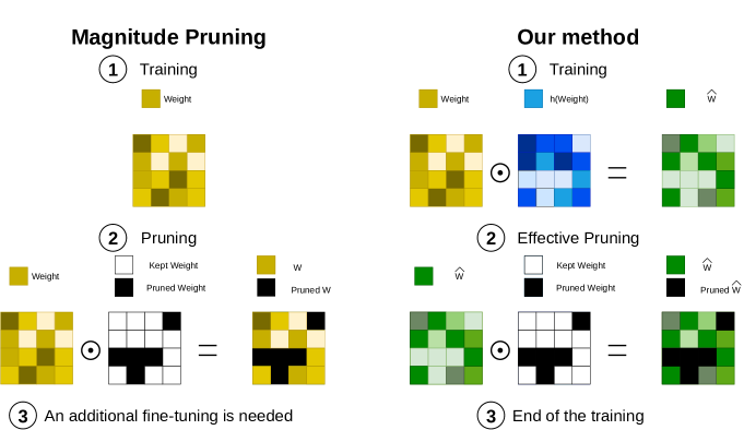
Fig. 1: Comparison of our method and magnitude pruning. Magnitude pruning does not include any prior on the weights during the initial training phase and needs an additional fine-tuning procedure. Our method embeds a saliency heuristic based on the weight magnitude in the weight reparametrization and does not requires fine-tuning.

2 Proposed Method

Our reparametrization seeks to define a novel weight expression related to magnitude pruning [12, 14]. This expression corresponds to the Hadamard product involving a weight tensor and a function applied entry-wise to the same tensor (as shown in fig. 1). This function acts as a mask that $i)$ multiplies weights by soft-pruning factors which capture their importance and $ii)$ pushes less important weights to zero through a particular budget added to the cross entropy loss.
Our proposed framework allows for a joint optimization of the network weights and topology. On the one hand, it prevents disconnections which may lead to degenerate networks with irrecoverable performance drop. On the other hand, it allows reaching a targeted pruning budget in a more convenient way than $\ell_{1}$ regularization. Our reparametrization also helps minimizing the discrepancy between the primary and the surrogate networks by maintaining competitive performances without fine-tuning. Learning the surrogate network requires only one step that achieves pruning as a part of network design. This step zeroes out the targeted number of connections by constraining their reparametrized weights to vanish.

2.1 Weight reparametrization

Without a loss of generality, we consider $f$ as a primary network whose layers are recursively defined as

$$f(\mathbf{x})=g_{L}\big{(}\mathbf{w}_{L}g_{L-1}(\mathbf{w}_{L-1}g_{L-2}\dots\mathbf{w}_{2}g_{1}(\mathbf{w}_{1}\mathbf{x}))\big{)},$$ (1)

with $g_{\ell}$ being a nonlinear activation associated to $\ell\in\left\{1,\dots,L\right\}$ and $\left\{\mathbf{w}_{\ell}\right\}_{\ell}$ a weight tensor. Considering eq. 1, a surrogate network $g$ is defined as

$$g(\mathbf{x})=g_{L}\big{(}\mathbf{\hat{w}}_{L}g_{L-1}(\mathbf{\hat{w}}_{L-1}g_{L-2}\dots\mathbf{\hat{w}}_{2}g_{1}(\mathbf{\hat{w}}_{1}\mathbf{x}))\big{)}.$$ (2)

In the above equation, $\mathbf{\hat{w}}_{\ell}$, referred to as apparent weight, is a reparametrization of $\mathbf{w}_{\ell}$, that includes a prior on its saliency, as

$$\mathbf{\hat{w}}_{\ell}=\mathbf{w}_{\ell} \odot h_{t}(\mathbf{w}_{\ell}),$$ (3)

with $h_{t}$ being a function that enforces the prior that smallest weights should be removed from the network. In order to achieve this goal, $h_{t}$ should exhibit the following properties:

1. $\forall x\in\mathds{R},~{}~{}0\leq h_{t}(x)\leq 1$

2. $h_{t}(x)\in C^{1}\text{ on }\mathds{R}$

3. $h_{t}(x)=h_{t}(-x)$

4. $\forall a,\varepsilon\in\mathds{R}^{+\ast},~{}\exists~{}t\in\mathds{R}^{+\ast}~{}|~{}h_{t}(x)\leq\varepsilon,x\in[-a,a]$

The first property ensures that the reparametrization is neither changing the sign of the apparent weight, nor acting as a scaling factor greater than one. In other words, it acts as the identity for sufficiently large weights, and as a contraction factor for small ones. The second property is necessary to ensure that the reparametrization function has computable gradient while the third property states that $h_{t}$ should be symmetric in order to avoid any bias towards the positive and the negative weights, so only their magnitudes matter. The last property ensures the existence of a temperature parameter $t$ which allows upper-bounding the response of $h_{t}$ on any interval for any arbitrary $\varepsilon$. Hence, $h_{t}$ acts as a stopband filter which eliminates the smallest weights where the parameter $t$ controls the width of that filter.
In order to match a specific budget, the width of the stopband is tuned according to the weight distribution of each layer. Note that the manual setting of this parameter is difficult so in practice $t$ is learned as a part of gradient descent; the initial setting $t_{\text{init}}$ of this temperature is shown in table 1.
Considering the aforementioned four properties of $h_{t}$, a simple choice of that function is

$$h_{t}(x)=\exp\bigg{\{}{-\displaystyle\frac{1}{(tx)^{n}}}\bigg{\}},~{}n\in 2\mathds{N},$$ (4)

where $n$ controls the crispness of $h_{t}$. Although the function described in eq. 4 satisfies the four above properties, it suffers from numerical instability as it generates NaN (Not a Number) outputs in most of the widely used deep learning frameworks. We consider instead a stabilized variant with a similar behavior, as eq. 4, that still satisfies the four above properties (see also fig. 2). This numerically stable variant is defined as

$$h_{t}(x)=C_{1}\biggl{(}\text{exp}\bigg{\{}-\displaystyle\frac{1}{(tx)^{n}+1}\bigg{\}}-C_{2}\biggr{)},$$ (5)

with $C_{1}=\frac{1}{1-e^{-1}}$ and $C_{2}=e^{-1}$; the constant added to the denominator of the exponential prevents numerical instability. Note that the constants $C_{1}$ and $C_{2}$ are added to guarantee that $h_{t}$ satisfies the first property.

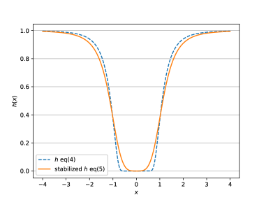
Fig. 2: An example of a reparametrization function and its numerically stabilized variant, with $t=1$ and $n=4$.

2.2 Budget Loss

Considering $C(\{\mathbf{w}_{1},\dots,\mathbf{w}_{L}\})$, $C_{\text{target}}$ as respectively the actual cost associated to a given network and the targeted one, the budget loss is defined as

$${\cal L}_{\text{budget}}=\bigl{(}C(\{\mathbf{w}_{1},\dots,\mathbf{w}_{L}\})-C_{\text{target}}\bigr{)}^{2}.$$ (6)

This budget loss is combined with the task classification loss. For a better conditioning of this combination, we normalize the budget loss by $C_{\text{initial}}$; the latter corresponds to the cost of the primary unpruned network and it is set in practice to the number of its parameters (see also section 3). Hence, eq. 6 is updated as

$${\cal L}_{\text{budget}}=\biggl{(}\displaystyle\frac{C(\{\mathbf{w}_{1},\dots,\mathbf{w}_{L}\})-C_{\text{target}}}{C_{\text{initial}}}\biggr{)}^{2}.$$ (7)

Finally, the two losses are combined together via a mixing parameter $\lambda>0$ that controls the relative importance of the budget, leading to

$${\cal L}={\cal L}_{\text{task}}+\lambda{\cal L}_{\text{budget}}.$$ (8)

Ideally, the budget of a neural network could be evaluated as the FLOPs needed for a forward pass or through the $\ell_{0}$ norm of its weights. However, neither is differentiable and therefore cannot be used in a gradient-based optimization. In order to address this issue, we use our weight reparametrization as a surrogate measure of $\ell_{0}$ and we define the cost function as

$$C(\{\mathbf{w}_{1},\dots,\mathbf{w}_{L}\})=\displaystyle\sum_{i=1}^{L}h(\mathbf{w}_{i}).$$ (9)

3 Experiments

In this section, we evaluate the accuracy of our method using Conv4, VGG19, and ResNet18 on the widely used CIFAR10 database and the TinyImageNet database [21]. The Conv4 model is similar to the network used by Frankle et al. in their Lottery Ticket experiments [22], as a smaller version of VGG19 introduced by Simonyan et al. [23] while ResNet18 is the small Residual Network of He et al. [24]. Comparisons w.r.t related state of the art are shown on the CIFAR10 and TinyImageNet datasets. CIFAR10 is composed of $60.000$ color images of $32\times 32$ pixels, divided into 10 classes. TinyImageNet is composed of $100.000$ color images of $64$ pixels divided into 200 classes. We use the default 2 fold setting for training and testing on both datasets.

3.1 Experimental setup

Unless stated differently, all the networks have been trained during 300 epochs with an initial learning rate of 0.1. A Reduce On Plateau policy is applied to the learning rate: if the test accuracy is not improving for 10 epochs in a row, then the learning rate is decreased by a factor 0.3. A weight decay is applied on the weights with a penalization factor of $5\times 10^{-5}$. An Early Stopping policy was used to stop prematurely the training if no improvement of the test accuracy is observed in 60 epochs. This procedure has been used both for initial training, and for fine-tuning of magnitude pruning (MP).
Performances are reported on the pruned networks: the latters are effectively pruned (extremely small weights are set to zero) up to the targeted pruning rate.

Network	Method	90%	95%	97%	99%
Dataset: CIFAR10
Conv4	Mag	54.94	22.91	13.1	13.07
	Mag+FT	89.50	87.38	85.57	76.7
	Ours	85.57	84.59	82.6	16.54
VGG19	Mag	10.0	10.0	10.0	10.0
	Mag+FT	93.57	93.52	92.96	10.0
	Ours	86.03	47.08	10.0	10.0
ResNet18	Mag	77.89	37.55	14.19	10.0
	Mag+FT	94.69	94.43	94.03	92.25
	Ours	91.59	89.89	33.49	15.08
Dataset: TinyImageNet
Conv4	Mag	26	10	3	0.5
	Mag+FT	45	45	43	21
	Ours	39	39	39	35

Table 1: Performances (accuracy) on the CIFAR10 and TinyImageNet test datasets for magnitude pruning (with and without fine-tuning) and our method, for different target pruning rates $p$. Our results are shown for $\lambda=5$, $n=4$, $t_{\text{init}}=100$ and $C_{\text{target}}=p\times C_{\text{initial}}$

3.2 Pruning performances

Table1 shows a comparison of our method against MP with and without fine-tuning. The performance is reported as the accuracy obtained on the test set of CIFAR10. For small networks such as Conv4, our method achieves compelling performances up to high pruning rates ($97$%) without any fine-tuning. The performances are within a few percent of fine-tuned MP (less than $4$% up to a pruning rate of $97$%), while providing a significant improvement w.r.t. the non fine-tuned version of MP (at least more than $30$% for pruning rates up to $97$%). For larger networks (namely VGG19 and ResNet18), the significant improvement over the non fine-tuned version of MP is still observed, although less pronounced. For high pruning rates, our method lags behind the fine-tuned version as shown in these results.

Observed performances in table 1 can be explained by analyzing the actual fraction of the remaining weights for the different targeted pruning rates shown in table 2. This fraction is obtained by dividing the actual cost of the network (once its training achieved) by the total number of its parameters. This cost is computed with our function defined in eq. 9. Table 2 shows that the targeted pruning is not always precisely reached, specifically for the most extreme (high) rates. When the targeted rate is not precisely reached, this has a strong negative impact on the effectively pruned networks. In contrast, when the targeted rate is reached, the test accuracy is either within a small margin (less than $0.5$%), or larger than the performances of the network trained with our method, before effective pruning. This is a significant improvement w.r.t. MP, which results into a dramatic drop in performance if fine-tuning is not applied. Results also show that our method successfully trains the weights while preparing the network for sparsity by reducing the magnitude of the less important weights. The performances of the networks trained with our method before effective pruning are reported in table 3 for the different targeted rates.

Finally, on TinyImageNet, our method remains stable w.r.t. different pruning rates and outperforms MP as well as fine-tuned MP by a significant margin, especially at the highest pruning rates.

Network	90%	95%	97%	99%
Conv4	0.10	0.05	0.03	0.03
VGG19	0.11	0.09	0.08	0.08
ResNet18	0.09	0.05	0.06	0.05

Table 2: Fraction of the remaining weights for targeted pruning rates on the CIFAR10 dataset, with $\lambda=5$, $n=4$ and $t_{\text{init}}=100$, computed with our surrogate cost function (cf eq. 9). Italics design fractions of the remaining weights that are in excess compared to the targeted pruning rate.

Network	90%	95%	97%	99%
Conv4	85.68	83.04	84.89	82.68
VGG19	88.65	88.07	88.89	89.19
ResNet18	91.62	91.01	90.42	90.71

Table 3: Performances (accuracy) on the CIFAR10 test dataset before effective pruning, for different target pruning rates, with $\lambda=5$, $n=4$ and $t_{\text{init}}=100$

4 Conclusion

We introduce in this paper a new budget-aware pruning method based on weight reparametrization. The latter acts as a regularizer that emphasizes on the most important connections in a given primary network while reaching a targeted cost and maintaining relatively close performances. Extensive experiments conducted on standard networks and datasets show that our method achieves compelling results without any fine-tuning. Moreover, while the targeted budget is satisfied, our method does not show any significant performance degradation even when enforced with an effective pruning step. Future work will investigate other classification tasks requiring surrogate networks with higher pruning rates and close performances w.r.t. the underlying primary networks. In particular online training on massive data (such as videos) is time demanding, and requires training cost-aware lightweight networks very efficiently.

Acknowledgment. This work has been achieved within a partnership between Sorbonne University (LIP6 Lab) and Netatmo.

References

- [1] Misha Denil, Babak Shakibi, Laurent Dinh, Marc’Aurelio Ranzato, and Nando de Freitas, “Predicting parameters in deep learning,” in NIPS, 2013, pp. 2148–2156.
- [2] Geoffrey E. Hinton, Oriol Vinyals, and Jeffrey Dean, “Distilling the knowledge in a neural network,” CoRR, vol. abs/1503.02531, 2015.
- [3] Sergey Zagoruyko and Nikos Komodakis, “Paying more attention to attention: Improving the performance of convolutional neural networks via attention transfer,” in ICLR, 2017.
- [4] Adriana Romero, Nicolas Ballas, Samira Ebrahimi Kahou, Antoine Chassang, Carlo Gatta, and Yoshua Bengio, “Fitnets: Hints for thin deep nets,” in ICLR, 2015.
- [5] Seyed-Iman Mirzadeh, Mehrdad Farajtabar, Ang Li, Nir Levine, Akihiro Matsukawa, and Hassan Ghasemzadeh, “Improved knowledge distillation via teacher assistant,” in IAAI, 2020, pp. 5191–5198.
- [6] Ying Zhang, Tao Xiang, Timothy M. Hospedales, and Huchuan Lu, “Deep mutual learning,” in CVPR, 2018, pp. 4320–4328.
- [7] Sungsoo Ahn, Shell Xu Hu, Andreas C. Damianou, Neil D. Lawrence, and Zhenwen Dai, “Variational information distillation for knowledge transfer,” in CVPR, 2019, pp. 9163–9171.
- [8] Emily L. Denton, Wojciech Zaremba, Joan Bruna, Yann LeCun, and Rob Fergus, “Exploiting linear structure within convolutional networks for efficient evaluation,” in NIPS, 2014, pp. 1269–1277.
- [9] Song Han, Huizi Mao, and William J. Dally, “Deep compression: Compressing deep neural network with pruning, trained quantization and huffman coding,” in ICLR, 2016.
- [10] Qian Lou, Lantao Liu, Minje Kim, and Lei Jiang, “AutoQB: AutoML for network quantization and binarization on mobile devices,” CoRR, vol. abs/1902.05690, 2019.
- [11] Benoit Jacob, Skirmantas Kligys, Bo Chen, Menglong Zhu, Matthew Tang, Andrew G. Howard, Hartwig Adam, and Dmitry Kalenichenko, “Quantization and training of neural networks for efficient integer-arithmetic-only inference,” in CVPR, 2018, pp. 2704–2713.
- [12] Yann LeCun, John S. Denker, and Sara A. Solla, “Optimal brain damage,” in NIPS, 1989, pp. 598–605.
- [13] Babak Hassibi and David G. Stork, “Second order derivatives for network pruning: Optimal brain surgeon,” in NIPS, 1992, pp. 164–171.
- [14] Song Han, Jeff Pool, John Tran, and William J. Dally, “Learning both weights and connections for efficient neural network,” in NIPS, 2015, pp. 1135–1143.
- [15] Ramchalam Kinattinkara Ramakrishnan, Eyyüb Sari, and Vahid Partovi Nia, “Differentiable mask for pruning convolutional and recurrent networks,” in CRV, 2020, pp. 222–229.
- [16] Hao Li, Asim Kadav, Igor Durdanovic, Hanan Samet, and Hans Peter Graf, “Pruning filters for efficient convnets,” in ICLR, 2017.
- [17] Sajid Anwar, Kyuyeon Hwang, and Wonyong Sung, “Structured pruning of deep convolutional neural networks,” ACM, vol. 13, no. 3, pp. 32:1–32:18, 2017.
- [18] Zhuang Liu, Jianguo Li, Zhiqiang Shen, Gao Huang, Shoumeng Yan, and Changshui Zhang, “Learning efficient convolutional networks through network slimming,” in ICCV, 2017, pp. 2755–2763.
- [19] Minsoo Kang and Bohyung Han, “Operation-aware soft channel pruning using differentiable masks,” in ICML, 2020, vol. 119 of Proceedings of Machine Learning Research, pp. 5122–5131.
- [20] Babak Hassibi, David G. Stork, and Gregory J. Wolff, “Optimal brain surgeon and general network pruning,” in ICNN, 1993, pp. 293–299.
- [21] Stanford CS231N, “TinyImageNet dataset,” http://cs231n.stanford.edu/tiny-imagenet-200.zip.
- [22] Jonathan Frankle and Michael Carbin, “The lottery ticket hypothesis: Finding sparse, trainable neural networks,” in ICLR, 2019.
- [23] Karen Simonyan and Andrew Zisserman, “Very deep convolutional networks for large-scale image recognition,” in ICLR, 2015.
- [24] Kaiming He, Xiangyu Zhang, Shaoqing Ren, and Jian Sun, “Deep residual learning for image recognition,” in CVPR. 2016, pp. 770–778, IEEE Computer Society.