$\displaystyle C^{1}$-conforming variational discretization of the biharmonic wave equation

Abstract

Biharmonic wave equations are of importance to various applications including thin plate analyses. In this work, the numerical approximation of their solutions by a $\displaystyle C^{1}$-conforming in space and time finite element approach is proposed and analyzed. Therein, the smoothness properties of solutions to the continuous evolution problem is embodied. High potential of the presented approach for more sophisticated multi-physics and multi-scale systems is expected. Time discretization is based on a combined Galerkin and collocation technique. For space discretization the Bogner–Fox–Schmit element is applied. Optimal order error estimates are proven. The convergence and performance properties are illustrated with numerical experiments.

1 Introduction

In this work we propose and analyze a space-time finite element approximation by $\displaystyle C^{1}$-conforming in space and time discrete functions of the initial-boundary value problem for the biharmonic wave equation,

$$\displaystyle\partial_{tt}u(\mathbf{x},t)+\Delta^{2}u(\mathbf{x},t) \displaystyle=f(\mathbf{x},t), \displaystyle\text{in}\ \Omega\times\left(0,T\right],$$ (1.1a)

$$\displaystyle u(\mathbf{x},0) \displaystyle=u_{0}(\mathbf{x}), \displaystyle\text{in}\ \Omega,$$ (1.1b)

$$\displaystyle\partial_{t}u(\mathbf{x},0) \displaystyle=u_{1}(\mathbf{x}), \displaystyle\text{in}\ \Omega,$$ (1.1c)

$$\displaystyle u(\mathbf{x},t) \displaystyle=0, \displaystyle\text{on}\ \partial\Omega\times\left(0,T\right],$$ (1.1d)

$$\displaystyle\partial_{\mathbf{n}}u(\mathbf{x},t) \displaystyle=0, \displaystyle\text{on}\ \partial\Omega\times\left(0,T\right],$$ (1.1e)

for a bounded domain $\displaystyle\Omega\subset\mathbb{R}^{2}$. This model is encountered in the modeling of various physical phenomena, such as plate bending and thin plate elasticity. The dynamic theory of thin Kirchhoff–Love plates investigates the propagation of waves in the plates as well as standing waves and vibration modes. Moreover, the system (1.1) can be studied as a prototype model for more sophisticated Kirchhoff-type equations, such as the Euler–Bernoulli equation describing the deflection of viscoelastic plates.

The finite element discretization of fourth order differential operators in space has been subject to intensive research in the literature. The Bogner–Fox–Schmit (BFS) element [17] is a classical $\displaystyle C^{1}$-conforming thin plate element obtained by taking the tensor products of cubic Hermite splines. The discrete solutions are continuously differentiable on tensor product (rectangular) elements, which can be a serious drawback since it limits the applicability of the resulting finite element method. However, for geometries allowing tensor product discretization it is considered to be one of the most efficient elements for plate analysis, cf. [51, p. 153]. It is also a reasonably low order element for plates which is very simple to implement, in contrast with triangular elements which either use higher order polynomials, such as the Argyris element [8], or macro element techniques, such as the Clough–Tocher element [24]. Due to the appreciable advantages of the BFS element and our target to propose a $\displaystyle C^{1}$-conforming in space and time finite element approach for (1.1), the BFS element is applied here.

We note that the finite element approximation of the biharmonic operator continues to be an active field of research, for recent contributions, see, e.g. [21, 22, 25]. In particular, discretization methods that support polyhedral meshes (the mesh cells can be polyhedra or have a simple shape but contain hanging nodes) and hinge on the primal formulation of the biharmonic equation leading to a symmetric positive definite system matrix are currently focused. These methods can be classified into three groups, depending on the dimension of the smallest geometric object to which discrete unknowns are attached. This criterion influences the stencil of the method. Furthermore, it has an impact on the level of conformity that can be achieved for the discrete solution. The methods in the first group were developed for the case where $\displaystyle\Omega\subset\mathbb{R}^{2}$. They attach discrete unknowns to the mesh vertices, edges, and cells and can achieve $\displaystyle C^{1}$-conformity. Salient examples are the $\displaystyle C^{1}$-conforming virtual element methods (VEM) from [20, 23] and the $\displaystyle C^{0}$-conforming VEM from [49]. Another example is the nonconforming VEM from [19, 50]. The methods in the second group attach discrete unknowns only to the mesh faces and cells for $\displaystyle\Omega\subset\mathbb{R}^{d}$, with $\displaystyle d\geq 2$. They admit static condensation, and provide a nonconforming approximation to the solution. The two salient examples are the weak Galerkin methods from [42, 48, 47] and the hybrid high-order method from [18]. Finally, the methods in the third group attach discrete unknowns only to the mesh cells and belong to the class of interior penalty discontinuous Galerkin methods. These are also nonconforming methods; cf. [41, 43, 29]. Important examples of nonconforming finite elements on simplicial meshes are the Morley element [40, 44] and the Hsieh–Clough–Tocher element (cf., e.g., [50, Chap. 6]). The spatial discretization of wave problems by discontinuous Galerkin methods has been focused further in the literature, cf., e.g.,[30, 7].

Among the most attractive methods for time discretization of second-order differential equations in time are the so-called continuous Galerkin or Galerkin–Petrov (cf., e.g., [9, 28, 36]) and the discontinuous Galerkin (cf., e.g., [32, 36]) schemes. For lowest order elements, these methods can be identified with certain well-known difference schemes, e.g. with the classical trapezoidal Newmark scheme (cf., e.g., [45, 46, 31]), the backward Euler scheme and the Crank–Nicolson scheme. Strong relations and equivalences between variational time discretizations, collocation methods and Runge–Kutta schemes have been observed. In the literature, the relations are exploited in the formulation and analysis of the schemes. For this we refer to, e.g., [2, 3]. Recently, variational time discretizations of higher order regularity in time [6, 13] have been devised for the second-order hyperbolic wave equations and analyzed carefully. In particular, optimal order error estimates are proved in [6, 13]. In [13], a $\displaystyle C^{1}$-conforming in time family of space-time finite element approximation that is based on a post-processing of the continuous in time Galerkin approximation is introduced. Concepts that are developed in [26] for first-order hyperbolic problems are transferred to the wave equation written as a first order system in time. In [13], a family of Galerkin–collocation approximation schemes with $\displaystyle C^{1}$- and $\displaystyle C^{2}$-regular in time discrete solutions are proposed and investigated by an optimal order error analysis and computational experiments. The conceptual basis of the families of approximations to the wave equation is the establishment of a connection between the Galerkin method for the time discretization and the classical collocation methods, with the perspective of achieving the accuracy of the former with reduced computational costs provided by the latter in terms of less complex algebraic systems. Further numerical studies for the wave equation can be found in [11, 5]. For the application of the Galerkin–collocation to mathematical models of fluid flow and systems of ordinary differential equations we refer to [4, 15, 16]. In the numerical experiments, the Galerkin–collocation schemes have proved their superiority over lower-order and standard difference schemes. In particular, energy conservation is ensured which is an essential feature for discretization schemes to second-order hyperbolic problems since the physics of solutions to the continuous problem are preserved.

As a logical consequence, for the biharmonic wave problem (1.1) it appears to be promising to combine the Galerkin–collocation time discretization with the BFS finite element discretization of the spatial variables to a $\displaystyle C^{1}$-conforming approximation in space and time. This is done here. We expect that the uniform variational approximation and higher order regularity will be advantageous for future applications in multi-physics systems based on (1.1) as a subproblem, the development of multi-scale approaches (in space and time) for (1.1) and the application of space-time adaptive methods. For the latter one, we refer to [10, 12, 37] for parabolic problems. In this work, we present the combined Galerkin–collocation and BFS finite element approximation of (1.1). Key ingredients of the construction of the Galerkin–collocation approach are the application of a special quadrature formula, proposed in [33], and the definition of a related interpolation operator for the right-hand side term of the variational equation. Both of them use derivatives of the given function. The Galerkin–collocation scheme relies in an essential way on the perfectly matching set of the polynomial spaces (trial and test space), quadrature formula, and interpolation operator. Then, a numerical error analysis is performed, optimal order error estimates are proved. Here, we restrict ourselves to presenting and stressing the differences to the wave equation for the Laplacian considered in [6]. Finally, a numerical study of the proposed discretization scheme is presented in order to illustrate the analyses.

This paper is organized as follows. In Section 2, we introduce our notation and formulate problem (1.1) as a first-order system in time. In Section 3, the Galerkin–collocation method is considered for time discretization. Some beneficial results for the error analysis are summarized in Section 4. In Section 5, we prove error estimates for the introduced Galerkin–collocation method for the plate vibration problem (1.1). Finally, in Section 6 we present a numerical study confirming the error estimates and perform a comparative study with only continuous in time approximations.

2 Preliminaries and notation

2.1 Evolution form

Throughout this paper, standard notation is used for Sobolev and Bochner spaces. By $\displaystyle B$ we denote a Banach space. We use $\displaystyle\left(\cdot,\cdot\right)$ for the $\displaystyle L^{2}(\Omega)$ inner product inducing the norm

$$\|\cdot\|=\|\cdot\|_{L^{2}(\Omega)}$$

and $\displaystyle\langle\cdot,\cdot\rangle$ for the duality pairing between a Hilbert space and its dual space. For the Sobolev norms we adopt the notation

$$\|\cdot\|_{m}=\|\cdot\|_{H^{m}(\Omega)}\quad\text{for}\,\,m\in\mathbb{N},\,m\geq 1$$

and further define the spaces

$$H=L^{2}(\Omega)\quad\text{and}\quad V=H^{2}_{0}(\Omega).$$

Let $\displaystyle V^{\prime}$ be the dual space of $\displaystyle V$. We introduce the operator $\displaystyle A:V\to V^{\prime}$ which for any given $\displaystyle u\in V$ is uniquely defined by

$$\langle Au,v\rangle=\left(\Delta u,\Delta v\right)\qquad\forall v\in V$$

and also the operator $\displaystyle\mathcal{L}:V\times H\to H\times V^{\prime}$ given by

$$\mathcal{L}=\begin{pmatrix}0&-I\\ A&0\end{pmatrix}.$$

Here $\displaystyle I$ is the identity operator that acts on $\displaystyle H$. For the error analysis, we define the energy norm on $\displaystyle H_{0}^{2}(\Omega)\times L^{2}(\Omega)$ by $\displaystyle|\!|\!|(w_{0},w_{1})|\!|\!|^{2}=\lVert\Delta w_{0}\rVert^{2}+\lVert w_{1}\rVert^{2}$.

In order to formulate problem (1.1) in an evolutionary form we further introduce the space

$$X:=L^{2}(0,T;V)\times L^{2}(0,T;H)$$

and set

$$u^{0}=u\qquad\text{and}\qquad u^{1}=\partial_{t}u.$$

With this notation then problem (1.1) can be equivalently stated as: Find $\displaystyle U=(u^{0},u^{1})\in X$ satisfying

$$\displaystyle\partial_{t}U+\mathcal{L}U \displaystyle=F\qquad\text{in}\quad(0,T)$$ (2.1a)

$$\displaystyle U(0) \displaystyle=U_{0}$$ (2.1b)

where $\displaystyle f\in L^{2}(0,T;H)$ is given, $\displaystyle F=(0,f)$ and $\displaystyle U_{0}=(u_{0},u_{1})$.

The existence and uniqueness of solutions to (2.1) is a classical result, cf. [38, p. 273, Thm. 1.1], and [39, p. 275, Thm. 8.2]. Further, we have the following regularity result $\displaystyle H^{2}(\Omega)\subset\subset C(\overline{\Omega})$ for $\displaystyle\Omega\subset\mathbb{R}^{2}$, cf. [1].

2.2 Time discretization

Our aim is to replace the time interval with a discrete time mesh and subsequently to iteratively compute the solution of (1.1) in the time nodes. For this reason, we split $\displaystyle I=\left(0,T\right]$ into $\displaystyle N\in\mathbb{N}$ time subintervals

$$\displaystyle I_{n} \displaystyle=\left(t_{n-1},t_{n}\right],\qquad n=1,\ldots,N,$$

where $\displaystyle 0=t_{0}<t_{1}<\cdots<t_{N}=T$ and introduce the time step parameter $\displaystyle\tau=\max_{n=1,\dots,N}\tau_{n}$, where $\displaystyle\tau_{n}=t_{n}-t_{n-1}$. The set $\displaystyle\mathcal{M}_{\tau}:=\{I_{1},\ldots,I_{N}\}$ of time intervals represents the time mesh. For simplicity, we use $\displaystyle I_{0}=\{t_{0}\}$.

We denote the space of all $\displaystyle B$-valued polynomials in time of order $\displaystyle k\in\mathbb{N}_{0}$ over a given interval $\displaystyle I_{n}$ by

$$\mathbb{P}_{k}(I_{n};B)=\left\{w_{\tau}:I_{n}\to B:w_{\tau}(t)=\sum_{j=0}^{k}W^{j}t^{j},\;\forall t\in I_{n},\;W^{j}\in B\;\forall j\right\}.$$

Moreover, for an integer $\displaystyle k\in\mathbb{N}$ we introduce the space of globally continuous functions in time, $\displaystyle X_{\tau}^{k}(B)$, and the space of global $\displaystyle L^{2}$-functions in time, $\displaystyle Y_{\tau}^{k}(B)$, as follows

$$\displaystyle X_{\tau}^{k}(B) \displaystyle:=\left\{w_{\tau}\in C(\bar{I};B):w_{\tau}\big{|}_{I_{n}}\in\mathbb{P}_{k}(I_{n};B)\;\,\forall I_{n}\in\mathcal{M}_{\tau}\right\},$$

$$\displaystyle Y_{\tau}^{k}(B) \displaystyle:=\left\{w_{\tau}\in L^{2}(I;B):w_{\tau}\big{|}_{I_{n}}\in\mathbb{P}_{k}(I_{n};B)\;\,\forall I_{n}\in\mathcal{M}_{\tau}\right\}.$$

We designate

$$\partial_{t}^{s}w(t_{n}^{+}):=\lim_{t\rightarrow t_{n}^{+0}}\partial_{t}^{s}w(t)\quad\text{and}\quad\partial_{t}^{s}w(t_{n}^{-}):=\lim_{t\rightarrow t_{n}^{-0}}\partial_{t}^{s}w(t)$$

to be the one-sided limits of the $\displaystyle s$-th derivative of a piecewise sufficiently smooth with respect to the time mesh $\displaystyle\mathcal{M}_{\tau}$ function $\displaystyle w:I\to B$ where $\displaystyle s\in\mathbb{N}_{0}$.

3 Discretizations of space and time

3.1 Space discretization

Let $\displaystyle\mathcal{T}_{h}$ be a shape-regular mesh of the spatial domain $\displaystyle\Omega$ with $\displaystyle h>0$ denoting the mesh size and let

$$V_{h}=\left\{v_{h}\in C^{1}(\Omega):v_{h}\big{|}_{T}\in\mathbb{Q}_{3}(T),v_{h}\big{|}_{\partial\Omega}=0,\,\partial_{\mathbf{n}}v_{h}\big{|}_{\partial\Omega}=0\ \forall T\in\mathcal{T}_{h}\right\}$$

be the finite element space built on the mesh using the Bogner–Fox–Schmit element. Here $\displaystyle\mathbb{Q}_{3}(T)$ denotes the set of all polynomials with maximum degree $\displaystyle 3$ in each variable.

We denote the $\displaystyle L^{2}$-orthogonal projection onto $\displaystyle V_{h}$ by $\displaystyle P_{h}$, i.e.,

$$(P_{h}w,v_{h})=(w,v_{h})\qquad\forall v_{h}\in V_{h}$$

and define the elliptic operator $\displaystyle R_{h}:V\to V_{h}$ via

$$(\Delta R_{h}w,\Delta v_{h})=(\Delta w,\Delta v_{h})\qquad\forall v_{h}\in V_{h}.$$ (3.1)

For $\displaystyle w\in H^{s}\cap H_{0}^{2}$ we have the estimates

$$\|w-R_{h}w\|_{m}\leq Ch^{4-m}\|w\|_{4},\qquad 0\leq m\leq 3$$ (3.2)

and

$$\|\Delta(w-R_{h}w)\|_{m}\leq Ch^{2-m}\|w\|_{4},\qquad 0\leq m\leq 1$$

which follow directly from the interpolation error estimates given in [21] along with Cea’s lemma and the Aubin–Nitsche trick.

Further, we introduce the $\displaystyle L^{2}$-projection $\displaystyle\mathcal{P}_{h}:H\times H\to V_{h}\times V_{h}$ and the elliptic projection $\displaystyle\mathcal{R}_{h}:V\times V\to V_{h}\times V_{h}$ both of which are onto the product space $\displaystyle V_{h}\times V_{h}$ and also the discrete operator $\displaystyle A_{h}:V\to V_{h}$ for which it holds

$$\left(A_{h}w,v_{h}\right)=\left(\Delta w,\Delta v_{h}\right)\qquad\forall v_{h}\in V_{h}.$$ (3.3)

Therefore, if $\displaystyle w\in V\cap H^{4}(\Omega)$, we have

$$\left(A_{h}w,v_{h}\right)=\left(\Delta w,\Delta v_{h}\right)=\langle Aw,v_{h}\rangle\qquad\forall v_{h}\in V_{h}$$

or

$$A_{h}w=P_{h}Aw\qquad\text{for }w\in V\cap H^{4}(\Omega).$$

Moreover, for the operator $\displaystyle\mathcal{L}_{h}:V\times H\to V_{h}\times V_{h}$ defined as

$$\mathcal{L}_{h}=\begin{pmatrix}0&-P_{h}\\ A_{h}&0\end{pmatrix}$$ (3.4)

the following relation holds

$$\left(\mathcal{L}_{h}W,\Phi_{h}\right)=\left(-w^{1},\varphi_{h}^{0}\right)+\left(\Delta w^{0},\Delta\varphi_{h}^{1}\right)=\left(-w^{1},\varphi_{h}^{0}\right)+\langle Aw^{0},\varphi_{h}^{1}\rangle=\langle\mathcal{L}W,\Phi_{h}\rangle$$

for $\displaystyle W=(w^{0},w^{1})\in(V\cap H^{4}(\Omega))\times H$ and for all $\displaystyle\Phi_{h}=(\varphi_{h}^{0},\varphi_{h}^{1})\in V_{h}\times V_{h}$ which demonstrates the consistency of $\displaystyle\mathcal{L}_{h}$ on $\displaystyle(V\cap H^{4}(\Omega))\times H$, i.e.,

$$\mathcal{L}_{h}W=\mathcal{P}_{h}\mathcal{L}W.$$ (3.5)

Finally, an appropriate approximation in $\displaystyle V_{h}\times V_{h}$ of the initial value $\displaystyle U_{0}\in V\times H$ is denoted by $\displaystyle U_{0,h}$.

3.2 Numerical integration

The following makes use of the Hermite-type, Gauss and Gauss-Lobatto quadrature formulas which for a sufficiently regular function $\displaystyle g$ on the interval $\displaystyle\bar{I}_{n}=[t_{n-1},t_{n}]$ read as

$$\displaystyle Q_{n}^{H}(g) \displaystyle=\left(\frac{\tau_{n}}{2}\right)^{2}\hat{w}_{L}^{H}\partial_{t}g(t_{n-1}^{+})+\frac{\tau_{n}}{2}\sum_{s=1}^{k-1}\hat{w}_{s}^{H}g(t_{n,s}^{H})+\left(\frac{\tau_{n}}{2}\right)^{2}\hat{w}_{R}^{H}\partial_{t}g(t_{n}^{-}),$$ (3.6a)

$$\displaystyle Q_{n}^{G}(g) \displaystyle=\frac{\tau_{n}}{2}\sum_{s=1}^{k-1}\hat{w}_{s}^{G}g(t_{n,s}^{G}),$$ (3.6b)

$$\displaystyle\quad Q_{n}^{GL}(g) \displaystyle=\frac{\tau_{n}}{2}\sum_{s=1}^{k}\hat{w}_{s}^{GL}g(t_{n,s}^{GL}),$$ (3.6c)

respectively. Here, $\displaystyle t_{n,s}^{H}$, $\displaystyle t_{n,s}^{G}$ and $\displaystyle t_{n,s}^{GL}$ are the corresponding quadrature points on the interval while $\displaystyle\{\hat{w}_{L}^{H},\,\hat{w}_{R}^{H},\,\hat{w}_{s}^{H}\}$, $\displaystyle\hat{w}_{s}^{G}$ and $\displaystyle\hat{w}_{s}^{GL}$ denote the corresponding weights.

We also consider the global Hermite interpolation $\displaystyle I_{\tau}^{H}:C^{1}(\bar{I};B)\to X_{\tau}^{k}(B)$ defined as

$$I_{\tau}^{H}w\big{|}_{I_{n}}:=I_{n}^{H}(w\big{|}_{I_{n}})$$ (3.7)

for all $\displaystyle n=1,\ldots,N$ where $\displaystyle I_{n}^{H}:C^{1}(\bar{I}_{n};B)\to\mathbb{P}_{k}(\bar{I}_{n};B)$ denotes the local Hermite interpolation operator with respect to point values and first derivatives on the interval $\displaystyle\bar{I}_{n}$.

3.3 Space-time discretizations

In this subsection we introduce the discretization of the biharmonic wave problem (1.1) by a space-time finite element approach utilizing a Galerkin–collocation approximation (cf. [6]) of the time variable along with BFS element for the approximation in space. The time discretization combines Galerkin and collocation techniques. Moreover, for comparative studies and in order to analyze the impact of the discrete solution’s higher regularity in time on the accuracy of the numerical results, the standard continuous in time Galerkin–Petrov approach (cf., e.g., [28, 13]) is presented here briefly. Within the latter familiy of schemes, the Crank–Nicolson method is recovered for piecewise linear approximations.

3.3.1 The Galerkin–collocation method cGP-C${}^{1}(k)$

The variational time discretization for the plate vibration problem (1.1) is derived following the idea in [14, 6] and reads as follows:

Problem 3.1.

Let $\displaystyle U_{\tau,h}(t_{n-1}^{-})$ for $\displaystyle n>1$ and $\displaystyle U_{\tau,h}(t_{0}^{-})=U_{0,h}$ for $\displaystyle n=1$ be given. Find $\displaystyle U_{\tau,h}\big{|}_{I_{n}}\in(\mathbb{P}_{k}(I_{n};V_{h}))^{2}$ satisfying

$$\displaystyle U_{\tau,h}(t_{n-1}^{+}) \displaystyle=U_{\tau,h}(t_{n-1}^{-}),$$ (3.8a)

$$\displaystyle\partial_{t}U_{\tau,h}(t_{n-1}^{+}) \displaystyle=-\mathcal{L}_{h}U_{\tau,h}(t_{n-1}^{+})+\mathcal{P}_{h}F(t_{n-1}^{+}),$$ (3.8b)

$$\displaystyle\partial_{t}U_{\tau,h}(t_{n}^{-}) \displaystyle=-\mathcal{L}_{h}U_{\tau,h}(t_{n}^{-})+\mathcal{P}_{h}F(t_{n}^{-}),$$ (3.8c)

$$\displaystyle Q_{n}^{H}(\left(\partial_{t}U_{\tau,h},V_{\tau,h}\right)+\left(\mathcal{L}_{h}U_{\tau,h},V_{\tau,h}\right)) \displaystyle=Q_{n}^{H}(\left(F,V_{\tau,h}\right))$$ (3.8d)

for all $\displaystyle V_{\tau,h}\in(\mathbb{P}_{k-3}(I_{n};V_{h}))^{2}$.

The existence and uniqueness of a solution to Problem 3.1 has been discussed in [6], see also [14].

From the definition of the scheme it also follows that $\displaystyle U_{\tau,h}\in(C^{1}(\bar{I};V_{h}))^{2}$ and (3.8b) can be written as

$$\partial_{t}U_{\tau,h}(t_{n-1}^{+})=\partial_{t}U_{\tau,h}(t_{n-1}^{-}),$$

where $\displaystyle\partial_{t}U_{\tau,h}(t_{0}^{-})=-\mathcal{L}_{h}U_{0,h}+\mathcal{P}_{h}F(0)$ and, therefore, Problem 3.1 can be equivalently written as:

Problem 3.2.

Let $\displaystyle k\geq 3$ be fixed and be given the values $\displaystyle\left(u^{0}_{\tau,h}\big{|}_{I_{n-1}}(t_{n-1}),u^{1}_{\tau,h}\big{|}_{I_{n-1}}(t_{n-1})\right)\in V_{h}^{2}$ for $\displaystyle 1<n\leq N$ and $\displaystyle\left(u^{0}_{\tau,h}\big{|}_{I_{0}}(t_{0}),u^{1}_{\tau,h}\big{|}_{I_{0}}(t_{0})\right)=(u_{0,h},u_{1,h})$ for $\displaystyle n=1$. Then the Galerkin–collocation for $\displaystyle\left(u^{0}_{\tau,h}\big{|}_{I_{n}},u^{1}_{\tau,h}\big{|}_{I_{n}}\right)\in\mathbb{P}_{k}(I_{n};V_{h})^{2}$ is defined as

$$\displaystyle\partial_{t}^{s}u^{0}_{\tau,h}\big{|}_{I_{n}}(t_{n-1}) \displaystyle=\partial_{t}^{s}u^{0}_{\tau,h}\big{|}_{I_{n-1}}(t_{n-1}),\quad s\in\{0,1\},$$ (3.9a)

$$\displaystyle\partial_{t}^{s}u^{1}_{\tau,h}\big{|}_{I_{n}}(t_{n-1}) \displaystyle=\partial_{t}^{s}u^{1}_{\tau,h}\big{|}_{I_{n-1}}(t_{n-1}),\quad s\in\{0,1\},$$ (3.9b)

$$\displaystyle\partial_{t}u^{0}_{\tau,h}\big{|}_{I_{n}}(t_{n})-u^{1}_{\tau,h}\big{|}_{I_{n}}(t_{n}) \displaystyle=0,$$ (3.9c)

$$\displaystyle\partial_{t}u^{1}_{\tau,h}\big{|}_{I_{n}}(t_{n})+{A}_{h}u^{0}_{\tau,h}\big{|}_{I_{n}}(t_{n}) \displaystyle=f(t_{n}),$$ (3.9d)

and

$$\displaystyle\int_{I_{n}}\int_{\Omega}\partial_{t}u^{0}_{\tau,h}\,\varphi^{0}_{\tau,h}-u^{1}_{\tau,h}\,\varphi^{0}_{\tau,h}\,\mathrm{d}\mathbf{x}\,\mathrm{d}t \displaystyle=0,$$ (3.9e)

$$\displaystyle\int_{I_{n}}\int_{\Omega}\partial_{t}u^{1}_{\tau,h}\,\varphi^{1}_{\tau,h}+{A}_{h}u^{0}_{\tau,h}\,\varphi^{1}_{\tau,h}\,\mathrm{d}\mathbf{x}\,\mathrm{d}t \displaystyle=\int_{I_{n}}\int_{\Omega}f\,\varphi^{1}_{\tau,h}\,\mathrm{d}\mathbf{x}\,\mathrm{d}t,$$ (3.9f)

for all $\displaystyle\left(\varphi^{0}_{\tau,h},\varphi^{1}_{\tau,h}\right)\in(\mathbb{P}_{k-3}(I_{n};V_{h}))^{2}$.

The discrete initial values $\displaystyle(u_{0,h},u_{1,h})\in V_{h}^{2}$ are determined from the interpolation of the functions $\displaystyle(u_{0},u_{1})$. We use the interpolant $\displaystyle u_{1,h}$ for the value $\displaystyle\partial_{t}u^{0}_{\tau,h}(0)$ from (3.9a). In order to obtain an appropriate value for $\displaystyle\partial_{t}u^{1}_{\tau,h}(0)$ in (3.9b) we consider (1.1a) at time $\displaystyle t=0$ and interpolate the function

$$\displaystyle\partial_{t}u^{1}(\mathbf{x},0)=f(\mathbf{x},0)-\Delta^{2}u(\mathbf{x},0).$$

The collocation conditions ensure a reduction in the size of the test space which results in a smaller linear system of equations.

Next, we summarize a result for scheme (3.8) used in the error analysis, cf. [6].

Proposition 3.3.

Consider the solution $\displaystyle U_{\tau,h}\in(X_{\tau}^{k}(V_{h}))^{2}$ of Problem 3.1. It holds that

$$B_{n}^{GL}(U_{\tau,h},V_{\tau,h})=Q_{n}^{GL}(\left(I_{\tau}^{H}F,V_{\tau,h}\right))$$

for all $\displaystyle V_{\tau,h}\in(\mathbb{P}_{k-2}(I_{n};V_{h}))^{2}$ and for $\displaystyle n=1,\ldots,N$, where

$$B_{n}^{GL}(U_{\tau,h},V_{\tau,h})=Q_{n}^{GL}(\left(\partial_{t}U_{\tau,h},V_{\tau,h}\right)+\left(\mathcal{L}_{h}U_{\tau,h},V_{\tau,h}\right)).$$

3.3.2 The cGP($\displaystyle k$)-method

The second time discretization method for the dynamic plate vibration problem considered is the Crank–Nicolson method [27]. The differential equation is solved iteratively by determining the solution at the time interval points $\displaystyle t_{n}$. To derive the Crank–Nicolson method, we use $\displaystyle\left(u^{0}_{\tau,h}\big{|}_{I_{n}},u^{1}_{\tau,h}\big{|}_{I_{n}}\right)\in\mathbb{P}_{k}(\overline{I}_{n};V_{h})^{2}$ and $\displaystyle\left(\varphi^{0}_{\tau,h}\big{|}_{I_{n}},\varphi^{1}_{\tau,h}\big{|}_{I_{n}}\right)\in\mathbb{P}_{k-1}(\overline{I}_{n};V_{h})^{2}$ as ansatz [6]. Since the solution space differs from the test space, this is referred to as a continuous Galerkin–Petrov method, or cGP($\displaystyle k$) for short. The discrete solution functions are globally continuous and use piecewise polynomials of degree $\displaystyle k$ for the time discretization. The cGP(1)-method corresponds to the Crank–Nicolson method.

In contrast to the Galerkin–collocation from the previous subsection, the Crank–Nicolson method only provides a solution that is continuous in time, but not a continuously differentiable solution.

4 Error analysis

Let us first note that the results from [35] for semilinear second order hyperbolic wave equations can be carried over to the plate vibration problem when $\displaystyle f=f(u)$, for more details see the appendix.

Next, we present several definitions required for the error analysis. Let $\displaystyle B\subset H$ and $\displaystyle l\in\mathbb{N}$. The local $\displaystyle L^{2}$-projections $\displaystyle\Pi_{n}^{l}:L^{2}(I_{n};B)\to\mathbb{P}_{l}(I_{n};B)$ are defined by

$$\int_{I_{n}}\left(\Pi_{n}^{l}w,q\right)\,\mathrm{d}t=\int_{I_{n}}\left(w,q\right)\,\mathrm{d}t\qquad\forall q\in\mathbb{P}_{l}(I_{n};B).$$

We consider the Hermite interpolant in time $\displaystyle I_{\tau}^{k+1}:C^{1}(\bar{I};B)\to C^{1}(\bar{I};B)\cap X_{\tau}^{k+1}(B)$ studied in [13, 26]. For this operator it is fulfilled that

$$I_{\tau}^{k+1}u(t_{n})=u(t_{n}),\quad\partial_{t}I_{\tau}^{k+1}u(t_{n})=\partial_{t}u(t_{n}),\quad n=0,\ldots,N,$$

and

$$I_{\tau}^{k+1}u(t_{n,\mu}^{GL})=u(t_{n,\mu}^{GL}),\quad n=1,\ldots,N,\,\mu=2,\ldots,k-1$$

and for a smooth function $\displaystyle u$, the following error estimates hold true on each interval $\displaystyle I_{n}$

$$\displaystyle\|\partial_{t}u-\partial_{t}I_{\tau}^{k+1}u\|_{C^{0}(\bar{I}_{n};B)} \displaystyle\leq C\tau_{n}^{k+1}\|u\|_{C^{k+2}(\bar{I}_{n};B)},$$

$$\displaystyle\|\partial_{t}^{2}u-\partial_{t}^{2}I_{\tau}^{k+1}u\|_{C^{0}(\bar{I}_{n};B)} \displaystyle\leq C\tau_{n}^{k}\|u\|_{C^{k+2}(\bar{I}_{n};B)}.$$

Moreover, we define the operator $\displaystyle R_{\tau}^{k}u\big{|}_{I_{n}}\in\mathbb{P}_{k}(I_{n};B)$ for $\displaystyle n=1,\ldots,N$ via the $\displaystyle(k+1)$ conditions

$$\displaystyle R_{\tau}^{k}u\big{|}_{I_{n}}(t_{n-1}) \displaystyle=I_{\tau}^{k+1}u(t_{n-1}),$$

$$\displaystyle\partial_{t}R_{\tau}^{k+1}u\big{|}_{I_{n}}(t_{n,s}) \displaystyle=\partial_{t}I_{\tau}^{k+1}u(t_{n,s}),\quad s=0,\ldots,k$$

and we set $\displaystyle R_{\tau}^{k}u(0):=u(0)$.

Here, we briefly summarize some of the properties of $\displaystyle R_{\tau}^{k}$ that are important for the analysis. Their proofs can be found in [13, 26].

Lemma 4.1.

Let $\displaystyle k\geq 3$. For $\displaystyle n=1,\ldots,N$ and $\displaystyle u\in C^{k+1}(\overline{I}_{n};B)$ the estimate

$$\displaystyle\lVert u-R_{\tau}^{k}u\rVert_{C^{0}(\overline{I}_{n};B)}\leq C\tau_{n}^{k+1}\lVert u\rVert_{C^{k+1}(\overline{I}_{n};B)}$$

holds.

A direct consequence of Lemma 4.1 is given in the following Corolllary.

Corollary 4.2.

For $\displaystyle n=1,\ldots,N$ and $\displaystyle u\in C^{k+1}(\overline{I}_{n};B)$ the estimate

$$\displaystyle\lVert\partial_{t}u-\partial_{t}R_{\tau}^{k}u\rVert_{C^{0}(\overline{I}_{n};B)}\leq C\tau_{n}^{k}\lVert u\rVert_{C^{k+1}(\overline{I}_{n};B)}$$ (4.1)

is fulfilled.

Next we consider the global Hermite interpolation operator defined in (3.7).

Lemma 4.3.

For $\displaystyle I_{\tau}^{H}:C^{1}(\bar{I};H)\to X_{\tau}^{k}(H)$ the following estimates

$$\displaystyle\|u-I_{\tau}^{H}u\|_{C^{0}(\bar{I}_{n};B)} \displaystyle\leq C\tau_{n}^{k+1}\|u\|_{C^{k+1}(\bar{I}_{n};B)}$$

$$\displaystyle\|\partial_{t}u-\partial_{t}I_{\tau}^{H}u\|_{C^{0}(\bar{I}_{n};B)} \displaystyle\leq C\tau_{n}^{k}\|u\|_{C^{k+1}(\bar{I}_{n};B)}$$

hold true for all $\displaystyle n=1,\ldots,N$ and all $\displaystyle u\in C^{k+1}(\bar{I}_{n};B)$.

Another important result for our analysis that has been proved in [13] is presented as follows.

Lemma 4.4.

Let us consider the Gauss quadrature formula (3.6b). For all polynomials $\displaystyle p\in\mathbb{P}_{k-1}(I_{n};B)$ and all $\displaystyle n=1,\ldots,N$ it is fulfilled that

$$\displaystyle\Pi_{\tau}^{k-2}p(t_{n,s}^{G})=p(t_{n,s}^{G}),\quad s=1,\ldots,k-1.$$

Finally, a useful norm bound, see [13, 26], is presented.

Lemma 4.5.

For any $\displaystyle u\in\mathbb{P}_{k}(I_{n};H)$ the following inequality

$$\int_{I_{n}}\|u\|^{2}\,\mathrm{d}t\leq C\tau_{n}\|u(t_{n-1})\|^{2}+\tau_{n}^{2}\int_{I_{n}}\|\partial_{t}u\|^{2}\,\mathrm{d}t.$$

is fulfilled.

5 Error estimates

Our ultimate goal in this section is to prove estimates for the error

$$E(t)=U(t)-U_{\tau,h}(t)=(e^{0}(t),e^{1}(t)),$$

where the Galerkin–collocation approximation $\displaystyle U_{\tau,h}$ is the solution of Problem 3.2 and $\displaystyle U(t)=(u^{0}(t),u^{1}(t))$. To achieve this, we start with estimations for $\displaystyle\partial_{t}E$ and afterwards we estimate the error $\displaystyle E$. Note that $\displaystyle E$ is continuously differentiable in time if $\displaystyle U\in(C^{1}(\overline{I};V))^{2}$ holds for the exact solution.

5.1 Error estimates for $\displaystyle\partial_{t}U_{\tau,h}$

First, we derive estimates for $\displaystyle\partial_{t}U_{\tau,h}$, which will be used later.

Theorem 5.1.

Let $\displaystyle U_{\tau,h}\in(X_{\tau}^{k}(V_{h}))^{2}$ be the discrete solution of Problem 3.1. Then, the time derivative $\displaystyle\partial_{t}U_{\tau,h}\in(X_{\tau}^{k-1}(V_{h}))^{2}$ solves for $\displaystyle n=1,\ldots,N$

$$\displaystyle B_{n}^{GL}(\partial_{t}U_{\tau,h},V_{\tau,h})=Q_{n}^{GL}(\left(\partial_{t}I_{\tau}^{H}F,V_{\tau,h}\right))=\int_{I_{n}}\left(\partial_{t}I_{\tau}^{H}F,V_{\tau,h}\right)\,\mathrm{d}t$$

for all $\displaystyle V_{\tau,h}\in(\mathbb{P}_{k-2}(I_{n};V_{h}))^{2}$.

Proof.

The proof differs from proof [6, Theorem 5.1] only in the definition of the operator $\displaystyle\mathcal{L}_{h}$. ∎

Lemma 5.2.

Let $\displaystyle U_{0,h}=(R_{h}u_{0},R_{h}u_{1})$. Then the identity

$$\displaystyle\partial_{t}U_{\tau,h}(0)=\begin{pmatrix}R_{h}&0\\ 0&P_{h}\end{pmatrix}\partial_{t}U(0).$$

holds.

Proof.

From $\displaystyle U_{\tau,h}(0)=U_{0,h}=(R_{h}u_{0},R_{h}u_{1})$ together with (3.8a) and (3.8b) for $\displaystyle n=1$ it follows

$$\displaystyle\partial_{t}U_{\tau,h}(0) \displaystyle=-\mathcal{L}_{h}U_{\tau,h}(0)+\mathcal{P}_{h}F(0)$$

$$\displaystyle=-\begin{pmatrix}0&-P_{h}\\ A_{h}&0\end{pmatrix}\begin{pmatrix}R_{h}u_{0}\\ R_{h}u_{1}\end{pmatrix}+\begin{pmatrix}0\\ P_{h}f(0)\end{pmatrix}=\begin{pmatrix}P_{h}R_{h}u_{1}\\ -A_{h}R_{h}u_{0}+P_{h}f(0)\end{pmatrix}.$$

Using the definition of the operator $\displaystyle R_{h}$, (3.1), we obtain

$$\displaystyle\left(A_{h}R_{h}u_{0},v_{h}\right)=\left(\Delta R_{h}u_{0},\Delta v_{h}\right)=\left(\Delta u_{0},\Delta v_{h}\right)=\langle Au_{0},v_{h}\rangle=\left(P_{h}Au_{0},v_{h}\right)$$

for all $\displaystyle v_{h}\in V_{h}$. Thus, $\displaystyle A_{h}R_{h}u_{0}=P_{h}Au_{0}$. In addition, we have

$$\displaystyle\left(P_{h}R_{h}u_{1},v_{h}\right)=\left(R_{h}u_{1},v_{h}\right)$$

for all $\displaystyle v_{h}\in V_{h}$, from which we infer $\displaystyle P_{h}R_{h}u_{1}=R_{h}u_{1}$. Thus, we have

$$\displaystyle\partial_{t}U_{\tau,h}(0)=\begin{pmatrix}R_{h}u_{1}\\ -P_{h}Au_{0}+P_{h}f(0)\end{pmatrix}$$

Calculating the right-hand side gives

$$\displaystyle\begin{pmatrix}R_{h}&0\\ 0&P_{h}\end{pmatrix}\partial_{t}U(0) \displaystyle=\begin{pmatrix}R_{h}&0\\ 0&P_{h}\end{pmatrix}(-\mathcal{L}U(0)+F(0))$$

$$\displaystyle=\begin{pmatrix}R_{h}&0\\ 0&P_{h}\end{pmatrix}\begin{pmatrix}u_{1}\\ -Au_{0}+f(0)\end{pmatrix}=\begin{pmatrix}R_{h}u_{1}\\ -P_{h}Au_{0}+P_{h}f(0)\end{pmatrix}.$$

This proves the statement. ∎

Theorem 5.3.

Let $\displaystyle\hat{u}$ be the solution of (1.1) with data $\displaystyle(\hat{f},\hat{u}_{0},\hat{u}_{1})$ instead of $\displaystyle(f,u_{0},u_{1})$. Furthermore, let $\displaystyle l\in\mathbb{N}$ and $\displaystyle\hat{f}_{\tau}$ be an approximation of $\displaystyle\hat{f}$ satisfying

$$\displaystyle\lVert\hat{f}-\hat{f}_{\tau}\rVert_{C(\overline{I}_{n};H)}\leq C_{\hat{f}}\tau_{n}^{l+1},\quad n=1,\ldots,N,$$

where $\displaystyle C_{\hat{f}}$ is independent of $\displaystyle n,N$ and $\displaystyle\tau_{n}$. Let $\displaystyle\hat{U}_{\tau,h}=(\hat{u}_{\tau,h}^{0},\hat{u}_{\tau,h}^{1})\in(X_{\tau}^{l}(V_{h}))^{2}$ denote the solution of the local perturbed cGP($\displaystyle l$)-cG($\displaystyle r$) problem

$$\displaystyle\int_{I_{n}}\left(\partial_{t}\hat{U}_{\tau,h},V_{\tau,h}\right)+\left(\mathcal{L}_{h}\hat{U}_{\tau,h},V_{\tau,h}\right)\,\mathrm{d}t=\int_{I_{n}}\left(\hat{F}_{\tau},V_{\tau,h}\right)\,\mathrm{d}t$$

for all test function $\displaystyle V_{\tau,h}=(v_{\tau,h}^{0},v_{\tau,h}^{1})\in(\mathbb{P}_{l-1}(I_{n};V_{h}))^{2}$ with $\displaystyle\hat{F}_{\tau}=(0,\hat{f}_{\tau})$ and initial value $\displaystyle\hat{U}_{\tau,h}(t_{n-1}^{+})=\hat{U}_{\tau,h}(t_{n-1}^{-})$ for $\displaystyle n>1$ and $\displaystyle\hat{U}_{\tau,h}(t_{0})=\hat{U}_{0,h}=(R_{h}\hat{u}_{0},P_{h}\hat{u}_{1})$. Then a sufficiently smooth exact solution $\displaystyle\hat{u}$ satisfies

$$\displaystyle\lVert\hat{u}(t)-\hat{u}_{\tau,h}^{0}(t)\rVert+\lVert\partial_{t}\hat{u}(t)-\hat{u}_{\tau,h}^{1}(t)\rVert\leq C(\tau^{l+1}C_{t}(\hat{u})+h^{4}C_{x}(\hat{u})),$$ (5.1)

$$\displaystyle\lVert\Delta(\hat{u}(t)-\hat{u}_{\tau,h}^{0}(t))\rVert\leq C(\tau^{l+1}C_{t}(\hat{u})+h^{2}C_{x}(\hat{u}))$$ (5.2)

for all $\displaystyle t\in\overline{I}$ where $\displaystyle C_{t}(\hat{u})$ and $\displaystyle C_{x}(\hat{u})$ depend on various temporal and spatial derivatives of $\displaystyle\hat{u}$.

Proof.

The proof follows the lines of the proof of [13, Theorem 5.5]. ∎

The main result in this section is

Theorem 5.4.

Let the exact solution $\displaystyle U=(u^{0},u^{1}):=(u,\partial_{t}u)$ be sufficiently smooth and $\displaystyle U_{0,h}:=(R_{h}u_{0},R_{h}u_{1})$, then the following estimates hold true for all $\displaystyle t\in\bar{I}$

$$\displaystyle\|\partial_{t}U(t)-\partial_{t}U_{\tau,h}(t)\| \displaystyle\leq C(\tau^{k}C_{t}(\partial_{t}u)+h^{4}C_{x}(\partial_{t}u))\leq C(\tau^{k}+h^{4}),$$ (5.3)

$$\displaystyle\|\Delta(\partial_{t}u^{0}(t)-\partial_{t}u_{\tau,h}^{0}(t))\| \displaystyle\leq C(\tau^{k}C_{t}(\partial_{t}u)+h^{2}C_{x}(\partial_{t}u))\leq C(\tau^{k}+h^{2}),$$ (5.4)

where the quantities $\displaystyle C_{t}(\partial_{t}u)$ and $\displaystyle C_{x}(\partial_{t}u)$ depend on various temporal and spatial derivatives of $\displaystyle\partial_{t}u$.

Proof.

This proof differs from proof [6, Theorem 5.5] in the definition of the operators $\displaystyle A$, $\displaystyle\mathcal{L}_{h}$ and $\displaystyle R_{h}$ as well as the finite element space $\displaystyle V_{h}$. Analogous to this proof in [6], estimates (5.3) and (5.4) follow from estimates (5.1) and (5.2). ∎

5.2 Error estimates for $\displaystyle U_{\tau,h}$

In this subsection we wish to estimate $\displaystyle U_{\tau,h}$. Therefore, we use the following splitting

$$\displaystyle E(t)=\Theta(t)+E_{\tau,h}(t)\quad\text{with}$$

$$\displaystyle\Theta(t)=U(t)-\mathcal{R}_{h}R_{\tau}^{k}U(t)\quad\text{and}\quad E_{\tau,h}(t)=\mathcal{R}_{h}R_{\tau}^{k}U(t)-U_{\tau,h}(t),$$

where $\displaystyle E_{\tau,h}(t)=(e_{\tau,h}^{0}(t),e_{\tau,h}^{1}(t))$.

Lemma 5.5 (Estimation of the interpolation error).

Let $\displaystyle m\in\{0,1\}$. Then, the error estimates

$$\displaystyle\lVert\Theta(t)\rVert_{m} \displaystyle\leq C(h^{4-m}+\tau_{n}^{k+1}), \displaystyle t\in\overline{I}_{n},$$ (5.5)

$$\displaystyle\lVert\partial_{t}\Theta(t)\rVert_{m} \displaystyle\leq C(h^{4-m}+\tau_{n}^{k}), \displaystyle t\in\overline{I}_{n},$$ (5.6)

are valid for $\displaystyle n=1,\ldots,N$ where $\displaystyle\lVert\cdot\rVert_{0}=\lVert\cdot\rVert$.

Proof.

First, we note that for the elliptic projection $\displaystyle R_{h}$ defined in (3.1) it holds that $\displaystyle\lVert R_{h}u\rVert\leq C\lVert\Delta R_{h}u\rVert\leq C\lVert\Delta u\rVert$. Then, the proof follows the same lines as the proof of [13, Lemma 5.7].

Using Lemma 4.1 and the approximation properties of the elliptic projection $\displaystyle R_{h}$ we obtain

$$\displaystyle\lVert\Theta(t)\rVert_{m} \displaystyle=\lVert U(t)-\mathcal{R}_{h}R_{\tau}^{k}U(t)\rVert_{m}$$

$$\displaystyle\leq\lVert U(t)-\mathcal{R}_{h}U(t)\rVert_{m}+\lVert\mathcal{R}_{h}(U(t)-R_{\tau}^{k}U(t))\rVert_{m}$$

$$\displaystyle\leq Ch^{4-m}\lVert U\rVert_{C^{0}(\overline{I};H^{4}(\Omega))}+\tau_{n}^{k+1}\lVert U\rVert_{C^{k+1}(\overline{I};H^{1}(\Omega))}$$

which proves (5.5). Applying estimate  (4.1) and the fact that $\displaystyle\partial_{t}$ and $\displaystyle R_{h}$ commute yields

$$\displaystyle\lVert\partial_{t}\Theta(t)\rVert_{m} \displaystyle\leq\lVert\partial_{t}U(t)-\mathcal{R}_{h}\partial_{t}U(t)\rVert_{m}+\lVert\mathcal{R}_{h}(\partial_{t}U(t)-\partial_{t}R_{\tau}^{k+1}U(t))\rVert_{m}$$

$$\displaystyle\leq Ch^{4-m}\lVert\partial_{t}U\rVert_{C^{0}(\overline{I};H^{4}(\Omega))}+C\tau_{n}^{k+1}\lVert U\rVert_{C^{k+2}(\overline{I};H^{1}(\Omega))}$$

which shows (5.6). ∎

Lemma 5.6 (Consistency error).

Let $\displaystyle U\in C^{1}(\overline{I};V)\times C^{1}(\overline{I};H)$. Then, we have

$$\displaystyle B_{n}^{GL}(E,V_{\tau,h})=Q_{n}^{GL}(\left(I_{\tau}^{GL}F-I_{\tau}^{H}F,V_{\tau,h}\right))=Q_{n}^{GL}(\left(F-I_{\tau}^{H}F,V_{\tau},h\right))$$

for all $\displaystyle V_{\tau,h}\in(Y_{\tau,h}^{k-2})^{2}$ and $\displaystyle n=1,\ldots,N$.

Proof.

Because of Proposition 3.3 and the consistency property (3.5), the proof differs from the proof [6, Lemma 5.7] only in the definition of the operators $\displaystyle\mathcal{L}$ and $\displaystyle\mathcal{L}_{h}$. ∎

For the proof of the following result we refer to [13, Lemma 5.9].

Lemma 5.7.

Let $\displaystyle p\in\mathbb{P}_{k}(I_{n})$ be an arbitrary polynomial of degree less than or equal to $\displaystyle k$. Then, the identity

$$\displaystyle\partial_{t}p(t_{n,\mu}^{G})=\partial_{t}I_{\tau}^{GL}p(t_{n,\mu}^{G})$$

is satisfied for all Gauss points $\displaystyle t_{n,\mu}^{G}\in I_{n},\mu=1,\ldots,k-1$.

Lemma 5.8 (Stability).

The following identity

$$\displaystyle\begin{aligned} &\quad B_{n}^{GL}((e_{\tau,h}^{0},e_{\tau,h}^{1}),(\Pi_{n}^{k-2}A_{h}I_{\tau}^{GL}e_{\tau,h}^{0},\Pi_{n}^{k-2}I_{\tau}^{GL}e_{\tau,h}^{1}))\\ &=\frac{1}{2}(\lVert\Delta e_{\tau,h}^{0}(t_{n})\rVert^{2}-\lVert\Delta e_{\tau,h}^{0}(t_{n-1})\rVert^{2}+\lVert e_{\tau,h}^{1}(t_{n})\rVert^{2}-\lVert e_{\tau,h}^{1}(t_{n-1})\rVert^{2})\end{aligned}$$

holds true for all $\displaystyle n=1,\ldots,N$.

Proof.

First, we note that $\displaystyle\left((e_{\tau,h}^{0},e_{\tau,h}^{1}),(\Pi_{n}^{k-2}A_{h}I_{\tau}^{GL}e_{\tau,h}^{0},\Pi_{n}^{k-2}I_{\tau}^{GL}e_{\tau,h}^{1})\right)\in\mathbb{P}_{2k-2}(I_{n};\mathbb{R})$. Using the Gauss-Lobatto interpolation operator, we obtain $\displaystyle I_{\tau}^{GL}e_{\tau,h}^{1}\in\mathbb{P}_{k-1}(I_{n};V_{h})$ and $\displaystyle A_{h}I_{\tau}^{GL}e_{\tau,h}^{0}\in\mathbb{P}_{k-1}(I_{n};V_{h})$. Then, we have

$$\displaystyle\begin{aligned} &\quad B_{n}^{GL}((e_{\tau,h}^{0},e_{\tau,h}^{1}),(\Pi_{n}^{k-2}A_{h}I_{\tau}^{GL}e_{\tau,h}^{0},\Pi_{n}^{k-2}I_{\tau}^{GL}e_{\tau,h}^{1}))\\ &=Q_{n}^{GL}(\left((\partial_{t}e_{\tau,h}^{0},\partial_{t}e_{\tau,h}^{1}),(\Pi_{n}^{k-2}A_{h}I_{\tau}^{GL}e_{\tau,h}^{0},\Pi_{n}^{k-2}I_{\tau}^{GL}e_{\tau,h}^{1})\right))\\ &\quad+Q_{n}^{GL}(\left((-P_{h}I_{\tau}^{GL}e_{\tau,h}^{1},A_{h}I_{\tau}^{GL}e_{\tau,h}^{0}),(\Pi_{n}^{k-2}A_{h}I_{\tau}^{GL}e_{\tau,h}^{0},\Pi_{n}^{k-2}I_{\tau}^{GL}e_{\tau,h}^{1})\right))\\ &=\int_{I_{n}}\left((\partial_{t}e_{\tau,h}^{0},\partial_{t}e_{\tau,h}^{1}),(\Pi_{n}^{k-2}A_{h}I_{\tau}^{GL}e_{\tau,h}^{0},\Pi_{n}^{k-2}I_{\tau}^{GL}e_{\tau,h}^{1})\right)\,\mathrm{d}t\\ &\quad+\int_{I_{n}}\left((-P_{h}I_{\tau}^{GL}e_{\tau,h}^{1},A_{h}I_{\tau}^{GL}e_{\tau,h}^{0}),(\Pi_{n}^{k-2}A_{h}I_{\tau}^{GL}e_{\tau,h}^{0},\Pi_{n}^{k-2}I_{\tau}^{GL}e_{\tau,h}^{1})\right)\,\mathrm{d}t\\ &=T_{1}+T_{2}.\end{aligned}$$ (5.7)

Using Lemma 4.4 together with the exactness of the $\displaystyle(k-1)$-point Gauss quadrature formula for polynomials on $\displaystyle\mathbb{P}_{2k-3}(I_{n};\mathbb{R})$ and subsequent application of Lemma 5.7, we obtain

$$\displaystyle\begin{aligned} T_{1}&=\int_{I_{n}}\left((\Pi_{n}^{k-2}\partial_{t}e_{\tau,h}^{0},\Pi_{n}^{k-2}\partial_{t}e_{\tau,h}^{1}),(\Pi_{n}^{k-2}A_{h}I_{\tau}^{GL}e_{\tau,h}^{0},\Pi_{n}^{k-2}I_{\tau}^{GL}e_{\tau,h}^{1})\right)\,\mathrm{d}t\\ &=Q_{n}^{G}(\left((\partial_{t}e_{\tau,h}^{0},\partial_{t}e_{\tau,h}^{1}),(A_{h}I_{\tau}^{GL}e_{\tau,h}^{0},I_{\tau}^{GL}e_{\tau,h}^{1})\right))\\ &=Q_{n}^{G}(\left((\partial_{t}I_{\tau}^{GL}e_{\tau,h}^{0},\partial_{t}I_{\tau}^{GL}e_{\tau,h}^{1}),(A_{h}I_{\tau}^{GL}e_{\tau,h}^{0},I_{\tau}^{GL}e_{\tau,h}^{1})\right))\\ &=\frac{\tau_{n}}{2}\sum_{\mu=1}^{k-1}\hat{w}_{\mu}^{G}\left(\partial_{t}I_{\tau}^{GL}e_{\tau,h}^{0}(t_{n,\mu}^{G}),A_{h}I_{\tau}^{GL}e_{\tau,h}^{0}(t_{n,\mu}^{G})\right)\\ &\quad+\frac{\tau_{n}}{2}\sum_{\mu=1}^{k-1}\hat{w}_{\mu}^{G}\left(\partial_{t}I_{\tau}^{GL}e_{\tau,h}^{1}(t_{n,\mu}^{G}),I_{\tau}^{GL}e_{\tau,h}^{1}(t_{n,\mu}^{G})\right)\\ &=\frac{\tau_{n}}{2}\sum_{\mu=1}^{k-1}\hat{w}_{\mu}^{G}\frac{1}{2}\mathrm{d}_{t}\lVert A_{h}^{1/2}I_{\tau}^{GL}e_{\tau,h}^{0}(t_{n,\mu}^{G})\rVert^{2}+\frac{\tau_{n}}{2}\sum_{\mu=1}^{k-1}\hat{w}_{\mu}^{G}\frac{1}{2}\mathrm{d}_{t}\lVert I_{\tau}^{GL}e_{\tau,h}^{1}(t_{n,\mu}^{G})\rVert^{2}.\end{aligned}$$

Using the exactness of the $\displaystyle(k-1)$-point Gauss quadrature formula on $\displaystyle\mathbb{P}_{2k-3}(I_{n};\mathbb{R})$ again, we obtain

$$\displaystyle\begin{aligned} T_{1}&=\int_{I_{n}}\left(\frac{1}{2}\mathrm{d}_{t}\lVert A_{h}^{1/2}I_{\tau}^{GL}e_{\tau,h}^{0}(t)\rVert^{2}+\frac{1}{2}\mathrm{d}_{t}\lVert I_{\tau}^{GL}e_{\tau,h}^{1}(t)\rVert^{2}\right)\,\mathrm{d}t\\ &=\frac{1}{2}\left(\lVert A_{h}^{1/2}e_{\tau,h}^{0}(t_{n})\rVert^{2}-\lVert A_{h}^{1/2}e_{\tau,h}^{0}(t_{n-1})\rVert^{2}+\lVert e_{\tau,h}^{1}(t_{n})\rVert^{2}-\lVert e_{\tau,h}^{1}(t_{n-1})\rVert^{2}\right).\end{aligned}$$ (5.8)

By using Lemma 4.4, we have that

$$\displaystyle\begin{aligned} T_{2}&=\int_{I_{n}}\left((-P_{h}I_{\tau}^{GL}e_{\tau,h}^{1},A_{h}I_{\tau}^{GL}e_{\tau,h}^{0}),(\Pi_{n}^{k-2}A_{h}I_{\tau}^{GL}e_{\tau,h}^{0},\Pi_{n}^{k-2}I_{\tau}^{GL}e_{\tau,h}^{1})\right)\,\mathrm{d}t\\ &=\int_{I_{n}}\left((-\Pi_{n}^{k-2}I_{\tau}^{GL}e_{\tau,h}^{1},\Pi_{n}^{k-2}A_{h}I_{\tau}^{GL}e_{\tau,h}^{0}),(\Pi_{n}^{k-2}A_{h}I_{\tau}^{GL}e_{\tau,h}^{0},\Pi_{n}^{k-2}I_{\tau}^{GL}e_{\tau,h}^{1})\right)\,\mathrm{d}t\\ &=\int_{I_{n}}\left(-\Pi_{n}^{k-2}I_{\tau}^{GL}e_{\tau,h}^{1},\Pi_{n}^{k-2}A_{h}I_{\tau}^{GL}e_{\tau,h}^{0}\right)+\left(\Pi_{n}^{k-2}A_{h}I_{\tau}^{GL}e_{\tau,h}^{0},\Pi_{n}^{k-2}I_{\tau}^{GL}e_{\tau,h}^{1}\right)\,\mathrm{d}t\\ &=0.\end{aligned}$$ (5.9)

Inserting the equations (5.8) and (5.9) into (LABEL:stabilityT) along with the identity $\displaystyle\lVert A_{h}^{1/2}v_{h}\rVert=\lVert\Delta v_{h}\rVert$ for $\displaystyle v_{h}\in V_{h}$ finally yields the assertion. ∎

Lemma 5.9 (Boundedness).

Let $\displaystyle V_{\tau,h}=(\Pi_{n}^{k-2}A_{h}I_{\tau}^{GL}e_{\tau,h}^{0},\Pi_{n}^{k-2}I_{\tau}^{GL}e_{\tau,h}^{1})$. Then the estimate

$$\displaystyle\lvert B_{n}^{GL}(\Theta,V_{\tau,h})\rvert\leq C\tau_{n}^{1/2}(\tau_{n}^{k+1}+h^{4})\{\tau_{n}\lVert E_{\tau,h}\rVert^{2}+\tau_{n}^{2}Q_{n}^{G}(\lVert\partial_{t}E_{\tau,h}\rVert^{2})\}^{1/2}$$

is valid for all $\displaystyle n=1,\ldots,N$.

Proof.

The proof of this lemma differs from that of [13, Lemma 5.11] only in the definition of the elliptic projection operator and the applied projection error estimates. ∎

Lemma 5.10 (Estimates on right-hand side term).

Let $\displaystyle V_{\tau,h}=(\Pi_{n}^{k-2}A_{h}I_{\tau}^{GL}e_{\tau,h}^{0},\Pi_{n}^{k-2}I_{\tau}^{GL}e_{\tau,h}^{1})$. Then, the estimation

$$\displaystyle Q_{n}^{GL}(\left((0,f-I_{\tau}^{H}f),V_{\tau,h}\right))\leq C\tau_{n}^{1/2}\tau_{n}^{k+1}\{\tau_{n}\lVert E_{\tau,h}(t_{n-1})\rVert^{2}+\tau_{n}^{2}Q_{n}^{G}(\lVert\partial_{t}E_{\tau,h}\rVert^{2})\}^{1/2}$$

is valid for $\displaystyle n=1,\ldots,N$.

Proof.

The proof differs from proof [6, Lemma 5.11] only in the definition of the operator $\displaystyle A_{h}$. ∎

Lemma 5.11 (Estimates on $\displaystyle E_{\tau,h}$).

Let $\displaystyle U_{0,h}=(R_{h},u_{0},R_{h},u_{1})$. Then

$$\displaystyle\lVert e_{\tau,h}^{0}(t_{n})\rVert_{1}^{2}+\lVert e_{\tau,h}^{1}\rVert^{2}\leq C\left(\tau^{k+1}+h^{4}\right)^{2}$$

holds true for all $\displaystyle n=1,\ldots,N$. Additionally,

$$\displaystyle\lVert\Delta e_{\tau,h}^{0}(t)\rVert \displaystyle\leq C(\tau^{k+1}+h^{3})$$

$$\displaystyle\lVert e_{\tau,h}^{0}(t)\rVert+\lVert e_{\tau,h}^{1}(t)\rVert \displaystyle\leq C(\tau^{k+1}+h^{4})$$

is statisfied for all $\displaystyle t\in\overline{I}$.

Proof.

The proof follows the lines of [6, Lemma 5.12]. ∎

Theorem 5.12 (Error estimate for $\displaystyle U_{\tau,h}$).

Let $\displaystyle U=(u,\partial_{t}u)$ be the solution of the problem (1.1) and $\displaystyle U_{\tau,h}$ be the discrete solution of problem (3.9) along with the initial condition $\displaystyle U_{0,h}=(R_{h}u_{0},R_{h}u_{1})$. Then the following estimates for the error $\displaystyle E(t)=(e^{0}(t),e^{1}(t))=U(t)-U_{\tau,h}(t)$ apply for all $\displaystyle t\in\overline{I}$:

$$\displaystyle\lVert e^{0}(t)\rVert+\lVert e^{1}(t)\rVert \displaystyle\leq C(\tau^{k+1}+h^{4}),$$

$$\displaystyle\lVert\Delta e^{0}(t)\rVert \displaystyle\leq C(\tau^{k+1}+h^{3}).$$

Additionally, the estimates

$$\displaystyle\lVert e^{0}\rVert_{L^{2}(I;H)}+\lVert e^{1}\rVert_{L^{2}(I;H)} \displaystyle\leq C(\tau^{k+1}+h^{4}),$$ (5.10)

$$\displaystyle\lVert\Delta e^{0}\rVert_{L^{2}(I;H)} \displaystyle\leq C(\tau^{k+1}+h^{3})$$

are satisfied.

Proof.

The proof of this theorem differs from the proof of [6, Theorem 5.13] only in the definition of the operators. ∎

6 Numerical experiments

The aim of the numerical experiments included in this section is:

• to compute the numerical convergence orders for the time discretizations discussed in the previous sections;

• to compare the solutions obtained when using the cGP-C${}^{1}(3)$-, the cGP($\displaystyle 2$)- and the Crank–Nicolson (cGP(1)-) method for time discretization.

The numerical experiments in the first part of this section are used to confirm the error estimates proven in Section 5 and to show the faster convergence of the cGP-C${}^{1}(3)$-method compared with the other algorithms investigated. In the second part of this section, we perform a comparative study in order to demonstrate the superiority of the cGP-C${}^{1}(3)$-method over the considered only continuous in time approximation schemes.

We assume that the spatial domain $\displaystyle\Omega\subset\mathbb{R}^{2}$ is either the unit square $\displaystyle(0,1)^{2}$ or the square $\displaystyle(-1,1)^{2}$ which during the discretization process has been partitioned as bisections of $\displaystyle N^{2}$ squares with mesh size $\displaystyle h=\sqrt{2}/N$ or $\displaystyle h=2\sqrt{2}/N$, respectively. Furthermore, we use the Bogner–Fox–Schmit element throughout for spatial discretization.

All the numerical tests included in this section have been conducted in NGSolve, see https://ngsolve.org.

6.1 Numerical convergence study

We will utilize the first example to provide numerical evidence for the error estimates proven in Section 5, on the one hand, and to present the better convergence properties of the cGP-C${}^{1}(3)$-method, on the other. For this purpose, we compare the experimental order of convergence of different time discretization schemes.

Thereby, we expect to obtain an order of convergence of 2 for the Crank-Nicolson (cGP(1)-) method, an order of 3 for the cGP(2)-method, and an order of 4 for the cGP-C${}^{1}(3)$-method. In addition, as in [13] for the wave equation, we expect to observe superconvergence for the cGP(2)-method in the discrete time points. While we predict a convergence order of 4 only in the discrete points for the cGP(2)-method, we anticipate a convergence order of 4 in all time points for the cGP-C${}^{1}(3)$-method.

In our first example, we solve system (1.1) for the spatial domain $\displaystyle\Omega=(0,1)^{2}$ and the temporal domain $\displaystyle I=(0,1)$. For a right-hand side

$$\displaystyle f(\mathbf{x},t) \displaystyle=-4\pi^{2}\sin(2\pi t)\cdot\sin^{2}(\pi x_{1})\cdot\sin^{2}(\pi x_{2})$$

$$\displaystyle\quad+\pi^{4}\sin(2\pi t)\cdot\left[16\sin^{2}(\pi x_{1})-8\right]\cdot\sin^{2}(\pi x_{2})$$

$$\displaystyle\quad+2\pi^{4}\sin(2\pi t)\left[2-4\sin^{2}(\pi x_{1})\right]\cdot\left[2-4\sin^{2}(\pi x_{2})\right]$$

$$\displaystyle\quad+\pi^{4}\sin(2\pi t)\cdot\sin^{2}(\pi x_{1})\cdot\left[16\sin^{2}(\pi x_{2})-8\right]$$

and initial values

$$\displaystyle u_{0}(\mathbf{x}) \displaystyle=0,$$

$$\displaystyle u_{1}(\mathbf{x}) \displaystyle=2\pi\cdot\sin^{2}(\pi x_{1})\cdot\sin^{2}(\pi x_{2}),$$

the exact solution $\displaystyle u$ is given by

$$\displaystyle u(\mathbf{x},t)=\sin(2\pi t)\cdot\sin^{2}(\pi x_{1})\cdot\sin^{2}(\pi x_{2}).$$ (6.1)

The corresponding numerical solution of Problem (1.1) computed with the cGP-C${}^{1}(3)$-method for $\displaystyle\tau=0.01,\,h=\frac{\sqrt{2}}{10}$ is shown in Figure 1.

Figure 1: Numerical solution of Problem (1.1) for the function (6.1) when the cGP-C${}^{1}(3)$-method with parameters $\displaystyle\tau=0.01,\,h=\frac{\sqrt{2}}{10}$ is applied.

For a comparison of the solutions of different time discretization methods, we consider the norms

$$\displaystyle\lVert u-u_{\tau,h}\rVert_{L^{\infty}(L^{2})} \displaystyle=\max_{t\in[0,T]}\left(\int_{\Omega}\lvert u(\mathbf{x},t)-u_{\tau,h}(\mathbf{x},t)\rvert^{2}\,\mathrm{d}\mathbf{x}\right)^{\frac{1}{2}}$$

and

$$\displaystyle\lVert u-u_{\tau,h}\rVert_{L^{2}(L^{2})} \displaystyle=\left(\int_{I}\int_{\Omega}\lvert u(\mathbf{x},t)-u_{\tau,h}(\mathbf{x},t)\rvert^{2}\,\mathrm{d}\mathbf{x}\,\mathrm{d}t\right)^{\frac{1}{2}}.$$

In order to approximate the $\displaystyle\lVert\cdot\rVert_{L^{\infty}(L^{2})}$ norm, we first evaluate the maximum only in the discrete temporal points in which we have computed the discrete solution $\displaystyle u_{\tau,h}$ and denote this value by $\displaystyle\lVert\cdot\rVert_{L_{\tau}^{\infty}(L^{2})}$. Secondly, we determine the maximum by additionally evaluating the discrete solution in the time points

$$\displaystyle I_{\tau} \displaystyle=\{t_{n,j}:t_{n,j}=t_{n-1}+j\cdot\frac{1}{100}\cdot\tau_{n},\,j=1,\ldots,99,\,n=1,\ldots,N\},$$

which we denote by $\displaystyle\lVert\cdot\rVert_{L^{\infty}(L^{2})}$.

We compute both norms on a sequence of spatial and temporal meshes in order to determine the numerical convergence orders. We start with $\displaystyle\tau_{0}=0.1,\,h_{0}=\frac{\sqrt{2}}{5}$ and halve both after each pass. With $\displaystyle e_{\tau,h}$ we denote the error with time step $\displaystyle\tau$ and mesh size $\displaystyle h$, then the following formula

$$\displaystyle EOC=\log_{2}\left(\frac{e_{\tau,h}}{e_{\frac{\tau}{2},\frac{h}{2}}}\right)$$

is applied to compute the experimental order of convergence (EOC).

The discretization errors and the corresponding convergence orders for the Crank–Nicolson, cGP(2)- and cGP-C¹(3)-method in case of function (6.1) are presented in Table 6.1.

$\displaystyle\tau$	$\displaystyle h$	$\displaystyle\lVert u-u_{\tau,h}\rVert_{L_{\tau}^{\infty}(L^{2})}$	order	$\displaystyle\lVert u-u_{\tau,h}\rVert_{L^{\infty}(L^{2})}$	order	$\displaystyle\lVert u-u_{\tau,h}\rVert_{L^{2}(L^{2})}$	order
cGP(1)
$\displaystyle\tau_{0}/2^{0}$	$\displaystyle h_{0}/2^{0}$	3.296e-03	–	1.794e-02	–	9.081e-03	–
$\displaystyle\tau_{0}/2^{1}$	$\displaystyle h_{0}/2^{1}$	7.835e-04	2.07	4.794e-03	1.90	2.281e-03	1.99
$\displaystyle\tau_{0}/2^{2}$	$\displaystyle h_{0}/2^{2}$	1.877e-04	2.06	1.233e-03	1.96	5.746e-04	1.99
$\displaystyle\tau_{0}/2^{3}$	$\displaystyle h_{0}/2^{3}$	4.746e-05	1.98	3.080e-04	2.00	1.435e-04	2.00
$\displaystyle\tau_{0}/2^{4}$	$\displaystyle h_{0}/2^{4}$	1.194e-05	1.99	7.701e-05	2.00	3.589e-05	2.00
cGP(2)
$\displaystyle\tau_{0}/2^{0}$	$\displaystyle h_{0}/2^{0}$	1.058e-03	–	1.059e-03	–	8.369e-04	–
$\displaystyle\tau_{0}/2^{1}$	$\displaystyle h_{0}/2^{1}$	7.258e-05	3.87	1.063e-04	3.32	6.731e-05	3.64
$\displaystyle\tau_{0}/2^{2}$	$\displaystyle h_{0}/2^{2}$	4.553e-06	3.99	1.247e-05	3.09	6.635e-06	3.34
$\displaystyle\tau_{0}/2^{3}$	$\displaystyle h_{0}/2^{3}$	2.867e-07	3.99	1.510e-06	3.05	7.625e-07	3.12
$\displaystyle\tau_{0}/2^{4}$	$\displaystyle h_{0}/2^{4}$	1.798e-08	4.00	1.857e-07	3.02	9.310e-08	3.03
cGP-C1(3)
$\displaystyle\tau_{0}/2^{0}$	$\displaystyle h_{0}/2^{0}$	1.165e-03	–	1.231e-03	–	8.533e-04	–
$\displaystyle\tau_{0}/2^{1}$	$\displaystyle h_{0}/2^{1}$	8.141e-05	3.84	8.151e-05	3.92	5.673e-05	3.91
$\displaystyle\tau_{0}/2^{2}$	$\displaystyle h_{0}/2^{2}$	5.314e-06	3.94	5.314e-06	3.94	3.363e-06	4.08
$\displaystyle\tau_{0}/2^{3}$	$\displaystyle h_{0}/2^{3}$	2.998e-07	4.15	2.999e-07	4.15	2.005e-07	4.07
$\displaystyle\tau_{0}/2^{4}$	$\displaystyle h_{0}/2^{4}$	1.823e-08	4.04	1.824e-08	4.04	1.222e-08	4.04

Table 6.1: Numerical errors and convergence orders for the Crank–Nicolson (cGP(1)), cGP(2)- and cGP-C¹(3)-method for the function (6.1).

As seen from this table, the discretization errors for the cGP(2)- and the cGP-C${}^{1}(3)$-method are smaller than the corresponding values for the Crank–Nicolson method. Moreover, the cGP(2)-method with global continuous and piecewise quadratic functions gives higher convergence orders than the Crank–Nicolson method with piecewise linear functions. The cGP-C${}^{1}(3)$-method has the highest convergence orders in both norms of all the methods studied.

The numerical convergence orders in the $\displaystyle\lVert\cdot\rVert_{L^{2}(L^{2})}$ norm tend to $\displaystyle 2$ for the Crank–Nicolson method and for the cGP(2)-method to $\displaystyle 3$. In the $\displaystyle\lVert\cdot\rVert_{L_{\tau}^{\infty}(L^{2})}$ norm it can be seen even that the convergence order is $\displaystyle 4$ for the cGP(2)-method whereas it is $\displaystyle 2$ for the Crank–Nicolson algorithm. This observed superconvergence in the $\displaystyle\lVert\cdot\rVert_{L_{\tau}^{\infty}(L^{2})}$ norm is due to the evaluation in the Gauss-Lobatto points. Comparing the evaluation of the maximum only in the time points where we have computed the discrete solution as in $\displaystyle\lVert\cdot\rVert_{L_{\tau}^{\infty}(L^{2})}$ with the evaluation on a finer temporal mesh as performed with $\displaystyle\lVert\cdot\rVert_{L^{\infty}(L^{2})}$, verifies this superconvergence effect. For a more detailed study of the superconvergence in the case of the wave equation, we refer to, e.g., [13]. All convergence orders for the cGP-C¹(3)-method tend to 4. This confirms the convergence order proven in Theorem 5.12.

Consequently, we obtain better convergence results in all discrete time points for the cGP-C${}^{1}(3)$-method, although we have the same numerical costs in terms of degrees of freedom as for the cGP(2)-method.

6.2 Vibration in heterogeneous media

In this section, we want to show that the cGP-C${}^{1}(3)$-method is also applicable for more complex problems. Additionally, we stress the superiority of this method by analyzing and comparing the number of non-zero entries in the system matrix which is involved in the linear system of equations in every time step.

As a second example in this work, we consider the modified problem

$$\displaystyle\partial_{tt}u(\mathbf{x},t)+\Delta[c(\mathbf{x})\Delta u(\mathbf{x},t)] \displaystyle=f(\mathbf{x},t) \displaystyle\qquad\text{in}\ \Omega\times\left(0,T\right],$$ (6.2a)

$$\displaystyle u(\mathbf{x},0) \displaystyle=u_{0}(\mathbf{x}) \displaystyle\qquad\text{in}\ \Omega,$$ (6.2b)

$$\displaystyle\partial_{t}u(\mathbf{x},0) \displaystyle=u_{1}(\mathbf{x}) \displaystyle\qquad\text{in}\ \Omega,$$ (6.2c)

$$\displaystyle u(\mathbf{x},t) \displaystyle=0 \displaystyle\qquad\text{on}\ \partial\Omega\times\left(0,T\right],$$ (6.2d)

$$\displaystyle\partial_{\mathbf{n}}u(\mathbf{x},t) \displaystyle=0 \displaystyle\qquad\text{on}\ \partial\Omega\times\left(0,T\right],$$ (6.2e)

which arises from structural health monitoring and can be treated analogously. The coefficient $\displaystyle c>0$ encodes the stiffness of the involved materials. Here we use the setting

$$\displaystyle\Omega=(-1,1)^{2},\qquad T=\frac{3}{100},\qquad c(\mathbf{x})=\begin{cases}1,&\text{if }x_{2}<0.2,\\ 9,&\text{if }x_{2}\geq 0.2,\end{cases}\qquad f=0,$$

with the initial values

$$\displaystyle u_{0} \displaystyle=0.2\cdot\exp(-\lvert 10\cdot\mathbf{x}\rvert^{2})\cdot(1-x_{1}^{2})^{2}\cdot(1-x_{2}^{2})^{2},$$

$$\displaystyle u_{1} \displaystyle=0.$$

The first few time steps of the numerical solution of Problem (6.2) using the cGP-C${}^{1}(3)$-method are depicted in Figure 2.

Figure 2: First few time steps of the numerical solution of Problem (6.2) using the cGP-C${}^{1}(3)$ method with $\displaystyle\tau=0.01$.

We define the control region $\displaystyle\Omega_{c}=(0.75-l_{c},0.75+l_{c})\times(-l_{c},l_{c})$ with $\displaystyle l_{c}=1/32$ that simulates a senor and evaluate the expression

$$\displaystyle u_{c}(t)=\int_{\Omega_{c}}u_{\tau,h}(\mathbf{x},t)\,\mathrm{d}\mathbf{x}$$ (6.3)

there. Our first aim is to examine and compare the respective signals at the sensor for the three time discretization methods considered using different time step sizes. All calculations were performed with a fixed $\displaystyle 32\times 32$ spatial mesh discretization and a direct solver for the linear system of equations. In the following, we use the time step size $\displaystyle\tau=1/n_{t}$, where $\displaystyle n_{t}$ denotes the number of time intervals. The corresponding evaluations of the control quantity are depicted in Figure 3.

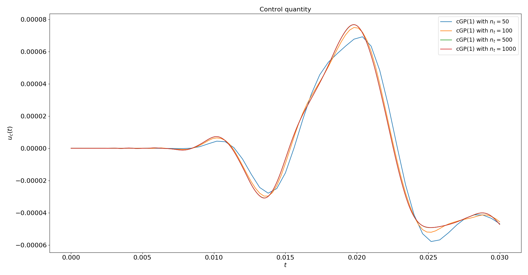
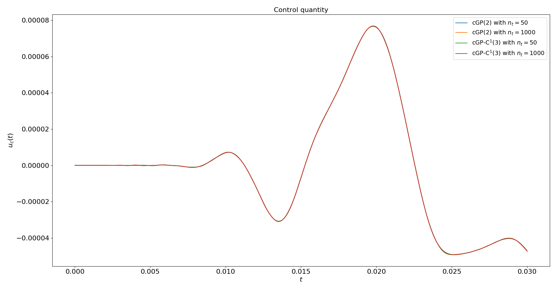
Figure 3: Evaluation of the control quantity (6.3) for the Crank–Nicolson (cGP(1)-), cGP(2)- and cGP-C${}^{1}(3)$-method with different time step sizes.

The Crank–Nicolson (cGP(1)-) method has lower accuracy in the control quantity (6.3), as can be seen in the upper graph in Figure 3. For large time step sizes, the curve of the control quantity deviates significantly from the curve we obtain for small time steps. In this example, the cGP(2)- and cGP-C${}^{1}(3)$-method have comparable accuracy, as shown in the bottom graph in Figure 3. Furthermore, we observe that both methods have high accuracy even for large time steps.

Next, we compare the number of non-zero entries in the system matrix resulting from each time discretization scheme. The number of non-zero entries (nze) as well as the number of degrees of freedom (dof) for the Crank–Nicolson, cGP(2)- and cGP-C${}^{1}(3)$-method are summarized in Table 6.2. The Crank–Nicolson method has fewer degrees of freedom and a smaller number of non-zero entries, but provides worse accuracy as already seen in the above example. Although the system matrices of the cGP(2)- and cGP-C${}^{1}(3)$-method have the same size, the cGP-C${}^{1}(3)$-method has fewer non-zero entries in the system matrix. This reduced number of non-zero entries is especially advantageous for the application of iterative solvers. We recall that both methods have the same order of convergence in the discrete time points as seen in the previous section. In [5], iterative solvers are applied for solving the linear systems of the cGP-C${}^{1}(3)$ approximation of the wave equation. In this case, a strong superiority of the cGP-C${}^{1}(3)$ approach over the cGP(2) one is observed with respect to accuracy and runtime of the simulations.

$\displaystyle|\mathcal{T}_{h}|$	cGP(1)		cGP(2)		cGP-C1(3)
	dof	nze	dof	nze	dof	nze
256	2312	1.4e+05	4624	5.0e+05	4624	3.6e+05
1024	8712	5.7e+05	17424	2.0e+06	17424	1.4e+06
4096	33800	2.3e+06	67600	7.9e+06	67600	5.7e+06
16384	133128	9.1e+06	266256	3.2e+07	266256	2.3e+07
65536	528392	3.7e+07	1056784	1.3e+08	1056784	9.3e+07
262144	2105352	1.5e+08	4210704	5.2e+08	4210704	3.8e+08

Table 6.2: Number of non-zero entries in the respective system matrix and number of degrees of freedom for the Crank–Nicolson (cGP(1)-), cGP(2)- and cGP-C${}^{1}(3)$-method using different spatial refinements.

7 Acknowledgement

The second and third authors acknowledge the support of this work by the Deutsche Forschungsgemeinschaft (DFG, German Research Foundation) as part of the project “Physics-oriented solvers for multicompartmental poromechanics” under grant number 456235063.

Appendix A Discrete formulation of the Galerkin–collocation

We consider (3.9) with $\displaystyle k=3$ which is the easiest case of Galerkin–collocation. We define the reference time interval $\displaystyle\hat{I}=[0,1]$ and the reference element transformation $\displaystyle F_{I_{n}}$ along with its inverse

$$\displaystyle F_{I_{n}}:\hat{I} \displaystyle\to\overline{I}_{n}, \displaystyle\qquad F_{I_{n}}(\hat{t}) \displaystyle=\tau_{n}\hat{t}+t_{n-1},$$

$$\displaystyle F_{I_{n}}^{-1}:\overline{I}_{n} \displaystyle\to\hat{I}, \displaystyle\qquad F_{I_{n}}^{-1}(t) \displaystyle=\frac{t-t_{n-1}}{\tau_{n}}.$$

Furthermore, we define the mass matrix $\displaystyle\mathbf{M}\in\mathbb{R}^{J\times J}$ and the operator matrix $\displaystyle\mathbf{A}\in\mathbb{R}^{J\times J}$

$$\displaystyle\mathbf{M}_{ij} \displaystyle=\int_{\Omega}\varphi_{i}\,\varphi_{j}\,\mathrm{d}\mathbf{x}, \displaystyle i,j=1,\ldots,J,$$ (A.1)

$$\displaystyle\mathbf{A}_{ij} \displaystyle=\int_{\Omega}\Delta\varphi_{i}\,\Delta\varphi_{j}\,\mathrm{d}\mathbf{x}, \displaystyle i,j=1,\ldots,J,$$ (A.2)

where $\displaystyle\varphi_{i},\,i=1,\ldots,J$ are the global space basis functions of $\displaystyle V_{h}$. Consider the one dimensional Bogner–Fox–Schmit element for the time discretization, then the temporal basis functions $\displaystyle\{\hat{\xi}_{k}\}_{k=0}^{3}\subset\mathbb{P}_{3}(\hat{I};\mathbb{R})$ on the reference element are given as

$$\displaystyle\begin{aligned} \hat{\xi}_{0}(\hat{t})&=1-3\hat{t}^{2}+2\hat{t}^{3},&\qquad\hat{\xi}_{1}(\hat{t})&=\hat{t}-2\hat{t}^{2}+\hat{t}^{3},\\ \hat{\xi}_{2}(\hat{t})&=3\hat{t}^{2}-2\hat{t}^{3},&\qquad\hat{\xi}_{3}(\hat{t})&=-\hat{t}^{2}+\hat{t}^{3}.\end{aligned}$$ (A.3)

We obtain the basis $\displaystyle\{\xi_{k}\}_{k=0}^{3}\subset\mathbb{P}_{3}(\overline{I}_{n};\mathbb{R})$ on the time interval $\displaystyle I_{n}$ by

$$\displaystyle\xi_{k}(t)=\hat{\xi}_{k}\left(F_{I_{n}}^{-1}(t)\right)\quad\forall t\in\overline{I}_{n},\,k=0,\ldots,3.$$ (A.4)

For the derivation of the Galerkin–collocation we require the integrals of the following basis functions

$$\displaystyle\int_{I_{n}}\xi_{0}\,\mathrm{d}t=\frac{\tau_{n}}{2},\qquad\int_{I_{n}}\xi_{1}\,\mathrm{d}t=\frac{\tau_{n}}{12},\qquad\int_{I_{n}}\xi_{2}\,\mathrm{d}t=\frac{\tau_{n}}{2},\qquad\int_{I_{n}}\xi_{3}\,\mathrm{d}t=-\frac{\tau_{n}}{12},$$ (A.5)

and also the integrals of the time derivatives

$$\displaystyle\int_{I_{n}}\partial_{t}\xi_{0}\,\mathrm{d}t=-1,\qquad\int_{I_{n}}\partial_{t}\xi_{1}\,\mathrm{d}t=0,\qquad\int_{I_{n}}\partial_{t}\xi_{2}\,\mathrm{d}t=1,\qquad\int_{I_{n}}\partial_{t}\xi_{3}\,\mathrm{d}t=0.$$ (A.6)

For the discrete functions $\displaystyle w_{\tau,h}\in\mathbb{P}_{3}(\overline{I}_{n};V_{h})$ we use the ansatz

$$\displaystyle\begin{aligned} w_{\tau,h}(\mathbf{x},t)&=\sum_{k=0}^{3}\sum_{j=1}^{J}w_{n,k,j}\,\varphi_{j}(\mathbf{x})\,\xi_{k}(t)=\sum_{k=0}^{3}w_{n,k}(\mathbf{x})\,\xi_{k}(t)\qquad\forall(\mathbf{x},t)\in\Omega\times\overline{I}_{n}\end{aligned}$$ (A.7)

with the space dependent coefficient functions $\displaystyle w_{n,k}(\mathbf{x})=\sum_{j=1}^{J}w_{n,k,j}\,\varphi_{j}(\mathbf{x})\in V_{h}$ and the constants $\displaystyle w_{n,k,j}\in\mathbb{R}$. For the test functions from $\displaystyle\mathbb{P}_{0}(\overline{I}_{n};V_{h})$ we use the basis

$$\displaystyle\mathcal{B}=\{\varphi_{1}\zeta_{0},\ldots,\varphi_{J}\zeta_{0}\},$$

where $\displaystyle\zeta_{0}\equiv 1$ on $\displaystyle\overline{I}_{n}$. To evaluate the source term $\displaystyle f$ in equation  (3.9f), we use the time interpolant $\displaystyle I_{\tau}^{H}f$, which is given on the interval $\displaystyle I_{n}$ by

$$\displaystyle\begin{aligned} I_{\tau}^{H}\big{|}_{I_{n}}f(t)&=f\big{|}_{I_{n}}(t_{n-1})\,\xi_{0}(t)+\tau_{n}\partial_{t}f\big{|}_{I_{n}}(t_{n-1})\,\xi_{1}(t)\\ &\quad+f\big{|}_{I_{n}}(t_{n})\,\xi_{2}(t)+\tau_{n}\partial_{t}f\big{|}_{I_{n}}(t_{n})\,\xi_{3}(t)\qquad\forall t\in\overline{I}_{n}.\end{aligned}$$ (A.8)

There $\displaystyle f\big{|}_{I_{n}}(t_{n-1})$ and $\displaystyle f\big{|}_{I_{n}}(t_{n})$ are to be understood as the corresponding one sided limit values.

We want now to derive the discrete formulation of the Galerkin–collocation (3.9) for the dynamic plate vibration problem (1.1). To do this, we consider first equation (3.9f). Due to the definition of the discrete operator $\displaystyle{A}_{h}$ from (3.3), it is equivalent to

$$\displaystyle\int_{I_{n}}\int_{\Omega}\partial_{t}u^{1}_{\tau,h}\,\varphi^{1}_{\tau,h}\,\mathrm{d}\mathbf{x}\,\mathrm{d}t+\int_{I_{n}}\int_{\Omega}\Delta u^{0}_{\tau,h}\,\Delta\varphi^{1}_{\tau,h}\,\mathrm{d}\mathbf{x}\,\mathrm{d}t=\int_{I_{n}}\int_{\Omega}f\,\varphi^{1}_{\tau,h}\,\mathrm{d}\mathbf{x}\,\mathrm{d}t.$$

Insertion of the basis representation (A.7) for $\displaystyle(u^{0}_{\tau,h},u^{1}_{\tau,h})\in\mathbb{P}_{3}(\overline{I}_{n};V_{h})^{2}$ and approximation of the source term function $\displaystyle f$ with the interpolant $\displaystyle I_{\tau}^{H}f$ yields

$$\displaystyle\begin{aligned} &\int_{I_{n}}\int_{\Omega}\partial_{t}\left(\sum_{k=0}^{3}u^{1}_{n,k}\,\xi_{k}\right)\,\varphi^{1}_{\tau,h}\,\mathrm{d}\mathbf{x}\,\mathrm{d}t+\int_{I_{n}}\int_{\Omega}\Delta\left(\sum_{k=0}^{3}u^{0}_{n,k}\,\xi_{k}\right)\,\Delta\varphi^{1}_{\tau,h}\,\mathrm{d}\mathbf{x}\,\mathrm{d}t\\ &\quad=\int_{I_{n}}\int_{\Omega}I_{\tau}^{H}f\ \varphi^{1}_{\tau,h}\,\mathrm{d}\mathbf{x}\,\mathrm{d}t.\end{aligned}$$ (A.9)

Subsequent separation of the time-dependent and space-dependent functions together with (A.6) results in

$$\displaystyle\int_{I_{n}}\int_{\Omega}\partial_{t}\left(\sum_{k=0}^{3}u^{1}_{n,k}\,\xi_{k}\right)\,\varphi^{1}_{\tau,h}\,\mathrm{d}\mathbf{x}\,\mathrm{d}t \displaystyle=\sum_{k=0}^{3}\left(\int_{I_{n}}\partial_{t}\xi_{k}\,\mathrm{d}t\int_{\Omega}u^{1}_{n,k}\,\varphi^{1}_{\tau,h}\,\mathrm{d}\mathbf{x}\right)$$

$$\displaystyle=\int_{\Omega}\left(-u^{1}_{n,0}+u^{1}_{n,2}\right)\,\varphi^{1}_{\tau,h}\,\mathrm{d}\mathbf{x}$$

for the first term. Analogously, application of (A.5) results in

$$\displaystyle\int_{I_{n}}\int_{\Omega}\Delta\left(\sum_{k=0}^{3}u^{0}_{n,k}\,\xi_{k}\right)\,\Delta\varphi^{1}_{\tau,h}\,\mathrm{d}\mathbf{x}\,\mathrm{d}t=\sum_{k=0}^{3}\left(\int_{I_{n}}\xi_{k}\,\mathrm{d}t\int_{\Omega}\Delta u^{0}_{n,k}\,\Delta\varphi^{1}_{\tau,h}\,\mathrm{d}\mathbf{x}\right)$$

$$\displaystyle\quad=\int_{\Omega}\Delta\left(\frac{\tau_{n}}{2}u^{0}_{n,0}+\frac{\tau_{n}}{12}u^{0}_{n,1}+\frac{\tau_{n}}{2}u^{0}_{n,2}-\frac{\tau_{n}}{12}u^{0}_{n,3}\right)\,\Delta\varphi^{1}_{\tau,h}\,\mathrm{d}\mathbf{x}$$

for the second term. On the right-hand side of (A.9) we obtain with the definition of the interpolant (A.8) in the same manner

$$\displaystyle\int_{I_{n}}\int_{\Omega}I_{\tau}^{H}f\ \varphi^{1}_{\tau,h}\,\mathrm{d}\mathbf{x}\,\mathrm{d}t$$

$$\displaystyle\quad=\int_{I_{n}}\int_{\Omega}\left(f(t_{n-1})\,\xi_{0}+\tau_{n}\partial_{t}f(t_{n-1})\,\xi_{1}+f(t_{n})\,\xi_{2}+\tau_{n}\partial_{t}f(t_{n})\,\xi_{3}\right)\,\varphi^{1}_{\tau,h}\,\mathrm{d}\mathbf{x}\,\mathrm{d}t$$

$$\displaystyle\quad=\int_{\Omega}\left(\frac{\tau_{n}}{2}f(t_{n-1})+\frac{\tau_{n}^{2}}{12}\partial_{t}f(t_{n-1})+\frac{\tau_{n}}{2}f(t_{n})-\frac{\tau_{n}^{2}}{12}\partial_{t}f(t_{n})\right)\,\varphi^{1}_{\tau,h}\,\mathrm{d}\mathbf{x}.$$

Next, we consider equation (3.9e)

$$\displaystyle\int_{I_{n}}\int_{\Omega}\partial_{t}u^{0}_{\tau,h}\,\varphi^{0}_{\tau,h}\,\mathrm{d}\mathbf{x}\,\mathrm{d}t-\int_{I_{n}}\int_{\Omega}u^{1}_{\tau,h}\,\varphi^{0}_{\tau,h}\,\mathrm{d}\mathbf{x}\,\mathrm{d}t=0.$$ (A.10)

Again we employ the basis representation (A.7) and obtain

$$\displaystyle\begin{aligned} \int_{I_{n}}\int_{\Omega}\partial_{t}u^{0}_{\tau,h}\,\varphi^{0}_{\tau,h}\,\mathrm{d}\mathbf{x}\,\mathrm{d}t&=\int_{I_{n}}\int_{\Omega}\partial_{t}\left(\sum_{k=0}^{3}u^{0}_{n,k}\,\xi_{k}\right)\,\varphi^{0}_{\tau,h}\,\mathrm{d}\mathbf{x}\,\mathrm{d}t=\int_{\Omega}\left(-u^{0}_{n,0}+u^{0}_{n,2}\right)\,\varphi^{0}_{\tau,h}\,\mathrm{d}\mathbf{x}\end{aligned}$$

for the first term and

$$\displaystyle\begin{aligned} \int_{I_{n}}\int_{\Omega}u^{1}_{\tau,h}\,\varphi^{0}_{\tau,h}\,\mathrm{d}\mathbf{x}\,\mathrm{d}t&=\int_{I_{n}}\int_{\Omega}\left(\sum_{k=0}^{3}u^{1}_{n,k}\,\xi_{k}\right)\,\varphi^{0}_{\tau,h}\,\mathrm{d}\mathbf{x}\,\mathrm{d}t\\ &=\int_{\Omega}\left(\frac{\tau_{n}}{2}u^{1}_{n,0}+\frac{\tau_{n}}{12}u^{1}_{n,1}+\frac{\tau_{n}}{2}u^{1}_{n,2}-\frac{\tau_{n}}{12}u^{1}_{n,3}\right)\,\varphi^{0}_{\tau,h}\,\mathrm{d}\mathbf{x}\end{aligned}$$

for the second, where we have again used (A.5) and (A.6).

Now we analyze the collocation condition (3.9d). We multiply the equation with a test function $\displaystyle\varphi^{3}_{\tau,h}\in V_{h}$ and integrate over the space domain. Using the definition of $\displaystyle A_{h}$, (3.3), condition (3.9d) is then equivalent to

$$\displaystyle\int_{\Omega}\partial_{t}u^{1}_{\tau,h}(t_{n})\,\varphi^{3}_{\tau,h}+\Delta u^{0}_{\tau,h}(t_{n})\,\Delta\varphi^{3}_{\tau,h}\,\mathrm{d}\mathbf{x} \displaystyle=\int_{\Omega}f(t_{n})\,\varphi^{3}_{\tau,h}\,\mathrm{d}\mathbf{x}.$$ (A.11)

Next, let us take a closer look at the function evaluations. Using (A.7), (A.3), (A.4) and the chain rule we obtain

$$\displaystyle\begin{aligned} \partial_{t}w_{\tau,h}(t_{n})&=\sum_{k=0}^{3}w_{n,k}(\mathbf{x})\,\partial_{t}\xi_{k}(t_{n})=\sum_{k=0}^{3}w_{n,k}(\mathbf{x})\,\partial_{\hat{t}}\hat{\xi}_{k}\left(F_{I_{n}}^{-1}(t_{n})\right)\frac{1}{\tau_{n}}\\ &=\sum_{k=0}^{3}w_{n,k}(\mathbf{x})\,\partial_{\hat{t}}\hat{\xi}_{k}(1)\frac{1}{\tau_{n}}=\frac{1}{\tau_{n}}w_{n,3}(\mathbf{x})\end{aligned}$$ (A.12)

for $\displaystyle w_{\tau,h}\in\mathbb{P}_{3}(\overline{I}_{n};V_{h})$. The same procedure delivers also the identity

$$\displaystyle\begin{aligned} w_{\tau,h}(t_{n})&=\sum_{k=0}^{3}w_{n,k}(\mathbf{x})\,\xi_{k}(t_{n})=\sum_{k=0}^{3}w_{n,k}(\mathbf{x})\,\hat{\xi}_{k}\left(F_{I_{n}}^{-1}(t_{n})\right)\\ &=\sum_{k=0}^{3}w_{n,k}(\mathbf{x})\,\hat{\xi}_{k}(1)=w_{n,2}(\mathbf{x}).\end{aligned}$$ (A.13)

Inserting (A.12) and (A.13) in (A.11) thus results in

$$\displaystyle\int_{\Omega}\frac{1}{\tau_{n}}u^{1}_{n,3}\,\varphi^{3}_{\tau,h}+\Delta u^{0}_{n,2}\,\Delta\varphi^{3}_{\tau,h}\,\mathrm{d}\mathbf{x} \displaystyle=\int_{\Omega}f(t_{n})\,\varphi^{3}_{\tau,h}\,\mathrm{d}\mathbf{x}.$$ (A.14)

The collocation condition (3.9c) reads as

$$\displaystyle\partial_{t}u^{0}_{\tau,h}(t_{n})-u^{1}_{\tau,h}(t_{n})=0.$$

This equation is multiplied with a test function $\displaystyle\varphi^{2}_{\tau,h}\in V_{h}$ and integrated over the space domain $\displaystyle\Omega$ to obtain the equation

$$\displaystyle\int_{\Omega}\partial_{t}u^{0}_{\tau,h}(t_{n})\,\varphi^{2}_{\tau,h}-u^{1}_{\tau,h}(t_{n})\,\varphi^{2}_{\tau,h}\,\mathrm{d}\mathbf{x} \displaystyle=0.$$ (A.15)

After that we use the identities (A.12) – (A.13) and insert them in equation (A.15). With this we conclude

$$\displaystyle\int_{\Omega}\frac{1}{\tau_{n}}u^{0}_{n,3}\,\varphi^{2}_{\tau,h}-u^{1}_{n,2}\,\varphi^{2}_{\tau,h}\,\mathrm{d}\mathbf{x} \displaystyle=0.$$ (A.16)

Overall, (A.9), (A.10), (A.14) and (A.16) lead to the system:

$$\displaystyle\begin{aligned} &\int_{\Omega}\left(-u^{0}_{n,0}+u^{0}_{n,2}\right)\,\varphi^{0}_{\tau,h}\,\mathrm{d}\mathbf{x}\\ &\quad-\int_{\Omega}\left(\frac{\tau_{n}}{2}u^{1}_{n,0}+\frac{\tau_{n}}{12}u^{1}_{n,1}+\frac{\tau_{n}}{2}u^{1}_{n,2}-\frac{\tau_{n}}{12}u^{1}_{n,3}\right)\,\varphi^{0}_{\tau,h}\,\mathrm{d}\mathbf{x}=0\end{aligned}$$ (A.17a)

$$\displaystyle\begin{aligned} &\int_{\Omega}\left(-u^{1}_{n,0}+u^{1}_{n,2}\right)\,\varphi^{1}_{\tau,h}\,\mathrm{d}\mathbf{x}\\ &\quad+\int_{\Omega}\Delta\left(\frac{\tau_{n}}{2}u^{0}_{n,0}+\frac{\tau_{n}}{12}u^{0}_{n,1}+\frac{\tau_{n}}{2}u^{0}_{n,2}-\frac{\tau_{n}}{12}u^{0}_{n,3}\right)\,\Delta\varphi^{1}_{\tau,h}\,\mathrm{d}\mathbf{x}\\ &=\int_{\Omega}\left(\frac{\tau_{n}}{2}f(t_{n-1})+\frac{\tau_{n}^{2}}{12}\partial_{t}f(t_{n-1})+\frac{\tau_{n}}{2}f(t_{n})-\frac{\tau_{n}^{2}}{12}\partial_{t}f(t_{n})\right)\,\varphi^{1}_{\tau,h}\,\mathrm{d}\mathbf{x}\end{aligned}$$ (A.17b)

$$\displaystyle\begin{aligned} \int_{\Omega}\frac{1}{\tau_{n}}u^{0}_{n,3}\,\varphi^{2}_{\tau,h}-u^{1}_{n,2}\,\varphi^{2}_{\tau,h}\,\mathrm{d}\mathbf{x}&=0\end{aligned}$$ (A.17c)

$$\displaystyle\begin{aligned} \int_{\Omega}\frac{1}{\tau_{n}}u^{1}_{n,3}\,\varphi^{3}_{\tau,h}+\Delta u^{0}_{n,2}\,\Delta\varphi^{3}_{\tau,h}\,\mathrm{d}\mathbf{x}&=\int_{\Omega}f(t_{n})\,\varphi^{3}_{\tau,h}\,\mathrm{d}\mathbf{x}\end{aligned}$$ (A.17d)

The remaining collocation conditions (3.9a) and (3.9b) yield the identities

$$\displaystyle u^{0}_{n,0}=u^{0}_{n-1,2},\qquad u^{0}_{n,1}=u^{0}_{n-1,3},\qquad u^{1}_{n,0}=u^{1}_{n-1,2},\qquad u^{1}_{n,1}=u^{1}_{n-1,3},$$

thereby reducing the number of unknowns.

Finally, we bring all known terms in (A.17) to the right side and on the time interval $\displaystyle[t_{n-1},t_{n}]$ search for the coefficient functions $\displaystyle\left(u^{0}_{n,2},u^{0}_{n,3},u^{1}_{n,2},u^{1}_{n,3}\right)\in V_{h}^{4}$ from the basis representation (A.7), which satisfy

$$\displaystyle\begin{aligned} &\int_{\Omega}u^{0}_{n,2}\,\varphi^{0}_{\tau,h}\,\mathrm{d}\mathbf{x}-\int_{\Omega}\left(\frac{\tau_{n}}{2}u^{1}_{n,2}-\frac{\tau_{n}}{12}u^{1}_{n,3}\right)\,\varphi^{0}_{\tau,h}\,\mathrm{d}\mathbf{x}\\ &\quad=\int_{\Omega}u^{0}_{n,0}\,\varphi^{0}_{\tau,h}\,\mathrm{d}\mathbf{x}+\int_{\Omega}\left(\frac{\tau_{n}}{2}u^{1}_{n,0}+\frac{\tau_{n}}{12}u^{1}_{n,1}\right)\,\varphi^{0}_{\tau,h}\,\mathrm{d}\mathbf{x}\end{aligned}$$ (A.18a)

$$\displaystyle\begin{aligned} &\int_{\Omega}u^{1}_{n,2}\,\varphi^{1}_{\tau,h}\,\mathrm{d}\mathbf{x}+\int_{\Omega}\Delta\left(\frac{\tau_{n}}{2}u^{0}_{n,2}-\frac{\tau_{n}}{12}u^{0}_{n,3}\right)\,\Delta\varphi^{1}_{\tau,h}\,\mathrm{d}\mathbf{x}\\ &\quad=\int_{\Omega}\left(\frac{\tau_{n}}{2}f(t_{n-1})+\frac{\tau_{n}^{2}}{12}\partial_{t}f(t_{n-1})+\frac{\tau_{n}}{2}f(t_{n})-\frac{\tau_{n}^{2}}{12}\partial_{t}f(t_{n})\right)\,\varphi^{1}_{\tau,h}\,\mathrm{d}\mathbf{x}\\ &\qquad+\int_{\Omega}u^{1}_{n,0}\,\varphi^{1}_{\tau,h}-\Delta\left(\frac{\tau_{n}}{2}u^{0}_{n,0}+\frac{\tau_{n}}{12}u^{0}_{n,1}\right)\,\Delta\varphi^{1}_{\tau,h}\,\mathrm{d}\mathbf{x}\end{aligned}$$ (A.18b)

$$\displaystyle\begin{aligned} \int_{\Omega}\frac{1}{\tau_{n}}u^{0}_{n,3}\,\varphi^{2}_{\tau,h}-u^{1}_{n,2}\,\varphi^{2}_{\tau,h}\,\mathrm{d}\mathbf{x}&=0\end{aligned}$$ (A.18c)

$$\displaystyle\begin{aligned} \int_{\Omega}\frac{1}{\tau_{n}}u^{1}_{n,3}\,\varphi^{3}_{\tau,h}+\Delta u^{0}_{n,2}\,\Delta\varphi^{3}_{\tau,h}\,\mathrm{d}\mathbf{x}&=\int_{\Omega}f(t_{n})\,\varphi^{3}_{\tau,h}\,\mathrm{d}\mathbf{x}\end{aligned}$$ (A.18d)

for all test functions $\displaystyle\left(\varphi^{0}_{\tau,h},\varphi^{1}_{\tau,h},\varphi^{2}_{\tau,h},\varphi^{3}_{\tau,h}\right)\in V_{h}^{4}$.

Using the definitions (A.1) and (A.2) of the mass matrix $\displaystyle\mathbf{M}$ and operator matrix $\displaystyle\mathbf{A}$, respectively we can write the system of equations (A.18) as a linear system of equations

$$\displaystyle\begin{aligned} \mathbf{M}\mathbf{u}^{0}_{n,2}-\mathbf{M}\left(\frac{\tau_{n}}{2}\mathbf{u}^{1}_{n,2}-\frac{\tau_{n}}{12}\mathbf{u}^{1}_{n,3}\right)=\mathbf{M}\mathbf{u}^{0}_{n,0}+\mathbf{M}\left(\frac{\tau_{n}}{2}\mathbf{u}^{1}_{n,0}+\frac{\tau_{n}}{12}\mathbf{u}^{1}_{n,1}\right)\end{aligned}$$ (A.19a)

$$\displaystyle\begin{aligned} &\quad\mathbf{M}\mathbf{u}^{1}_{n,2}+\mathbf{A}\left(\frac{\tau_{n}}{2}\mathbf{u}^{0}_{n,2}-\frac{\tau_{n}}{12}\mathbf{u}^{0}_{n,3}\right)\\ &=\mathbf{M}\left(\frac{\tau_{n}}{2}\mathbf{f}_{n,0}+\frac{\tau_{n}^{2}}{12}\mathbf{f}_{n,1}+\frac{\tau_{n}}{2}\mathbf{f}_{n,2}-\frac{\tau_{n}^{2}}{12}\mathbf{f}_{n,3}\right)\\ &\quad+\mathbf{M}\mathbf{u}^{1}_{n,0}-\mathbf{A}\left(\frac{\tau_{n}}{2}\mathbf{u}^{0}_{n,0}+\frac{\tau_{n}}{12}\mathbf{u}^{0}_{n,1}\right)\end{aligned}$$ (A.19b)

$$\displaystyle\frac{1}{\tau_{n}}\mathbf{M}\mathbf{u}^{0}_{n,3}-\mathbf{M}\mathbf{u}^{1}_{n,2} \displaystyle=\mathbf{0}$$ (A.19c)

$$\displaystyle\begin{aligned} \frac{1}{\tau_{n}}\mathbf{M}\mathbf{u}^{1}_{n,3}+\mathbf{A}\mathbf{u}^{0}_{n,2}&=\mathbf{M}\mathbf{f}_{n,2}.\end{aligned}$$ (A.19d)

We summarize the equations (A.19) more compactly. On the time interval $\displaystyle[t_{n-1},t_{n}]$ we search for the coefficient vector

$$\displaystyle\mathbf{x}=\left(\left(\mathbf{u}^{0}_{n,2}\right)^{\top},\left(\mathbf{u}^{0}_{n,3}\right)^{\top},\left(\mathbf{u}^{1}_{n,2}\right)^{\top},\left(\mathbf{u}^{1}_{n,3}\right)^{\top}\right)^{\top}\in\mathbb{R}^{4J}$$

as a solution of the linear system of equations

$$\displaystyle\mathbf{S}\mathbf{x}=\mathbf{b}$$

with matrix

$$\displaystyle\mathbf{S}=\begin{pmatrix}\mathbf{M}&\mathbf{0}&-\frac{\tau_{n}}{2}\mathbf{M}&\frac{\tau_{n}}{12}\mathbf{M}\\ \frac{\tau_{n}}{2}\mathbf{A}&-\frac{\tau_{n}}{12}\mathbf{A}&\mathbf{M}&\mathbf{0}\\ \mathbf{0}&\frac{1}{\tau_{n}}\mathbf{M}&-\mathbf{M}&\mathbf{0}\\ \mathbf{A}&\mathbf{0}&\mathbf{0}&\frac{1}{\tau_{n}}\mathbf{M}\end{pmatrix}\in\mathbb{R}^{4J\times 4J}$$

and right-hand side

$$\displaystyle\mathbf{b}=\begin{pmatrix}\mathbf{M}\left(\mathbf{u}^{0}_{n,0}+\frac{\tau_{n}}{2}\mathbf{u}^{1}_{n,0}+\frac{\tau_{n}}{12}\mathbf{u}^{1}_{n,1}\right)\\ b_{n,1}\\ \mathbf{0}\\ \mathbf{M}\mathbf{f}_{n,2}\end{pmatrix}\in\mathbb{R}^{4J},$$

where $\displaystyle b_{n,1}=\mathbf{M}\left(\frac{\tau_{n}}{2}\mathbf{f}_{n,0}+\frac{\tau_{n}^{2}}{12}\mathbf{f}_{n,1}+\frac{\tau_{n}}{2}\mathbf{f}_{n,2}-\frac{\tau_{n}^{2}}{12}\mathbf{f}_{n,3}+\mathbf{u}^{1}_{n,0}\right)-\mathbf{A}\left(\frac{\tau_{n}}{2}\mathbf{u}^{0}_{n,0}+\frac{\tau_{n}}{12}\mathbf{u}^{0}_{n,1}\right)$.

Appendix B Supplementary material

Recall $\displaystyle k\geq 3$. In the following, we consider Problem (1.1) with a Lipschitz continuous function $\displaystyle f(u)$ as right-hand side. Let $\displaystyle\mathcal{T}_{hn}$ be a partition of $\displaystyle\Omega$ on the time interval $\displaystyle I_{n}$. Then, we define the corresponding finite element space by

$$\displaystyle V_{h}^{n}=\left\{v_{h}\in C^{1}(\Omega):v_{h}\big{|}_{T}\in\mathbb{Q}_{3}(T),\,v_{h}\big{|}_{\partial\Omega}=0,\,\partial_{\mathbf{n}}v_{h}\big{|}_{\partial\Omega}=0\ \forall T\in\mathcal{T}_{hn}\right\}\cap H_{0}^{2}(\Omega)$$

with maximum diameter $\displaystyle h_{n}=\max_{K\in\mathcal{T}_{hn}}h_{K}$. Moreover, we will use the spaces

$$\displaystyle V_{k}^{n} \displaystyle=\left\{v:\Omega\times I_{n}\to\mathbb{R}:v\in\mathbb{P}_{k}(I_{n};V_{h}^{n})\right\},\quad V_{k}=\left\{v:\Omega\times\left(0,T\right]\to\mathbb{R}:v\big{|}_{I_{n}}\in V_{k}^{n}\right\}.$$

Analogous to (3.1), we define the elliptic operator $\displaystyle R_{h}^{n}:V\to V_{h}^{n}$ by

$$\displaystyle\left(\Delta R_{h}^{n}w,\Delta v_{h}\right)=\left(\Delta w,\Delta v_{h}\right)\qquad\forall v_{h}\in V_{h}^{n}.$$

We define $\displaystyle A_{h}^{n}:V\to V_{h}^{n}$ by

$$\left(A_{h}^{n}w,v_{h}\right)=(\Delta w,\Delta v_{h})\qquad\forall v_{h}\in V_{h}^{n}$$

and $\displaystyle\mathcal{L}_{h}^{n}:V\times H\to V_{h}^{n}\times V_{h}^{n}$ by

$$\displaystyle\mathcal{L}_{h}^{n}=\begin{pmatrix}0&-P_{h}^{n}\\ A_{h}^{n}&0\end{pmatrix}$$

analogous to (3.4), where $\displaystyle P_{h}^{n}$ is the $\displaystyle L^{2}$-projection onto $\displaystyle V_{h}^{n}$. Furthermore, we define

$$\displaystyle\Pi^{n}=\begin{pmatrix}R_{h}^{n}&0\\ 0&P_{h}^{n}\end{pmatrix}.$$

Now we can write our problem as: Find $\displaystyle U_{\tau,h}=(u_{\tau,h}^{0},u_{\tau,h}^{1})\in V_{k}\times V_{k}$ satisfying

$$\displaystyle\begin{aligned} \int_{I_{n}}(\partial_{t}U_{\tau,h},\Phi)+(\mathcal{L}_{h}^{n}U_{\tau,h},\Phi)\,\mathrm{d}t&=\int_{I_{n}}(F_{h}(U_{\tau,h}),\Phi)\,\mathrm{d}t,\quad\forall\Phi\in V_{k-1}^{n}\times V_{k-1}^{n},\\ U_{\tau,h}(t_{n-1}^{+})&=\Pi^{n}U_{\tau,h}(t_{n-1}),\quad n=1,\ldots,N,\end{aligned}$$ (B.1)

where $\displaystyle F_{h}(U_{\tau,h})=(0,P_{h}^{n}f(u_{\tau,h}^{0}))$ and $\displaystyle U_{\tau,h}(t_{0})=(u_{0},u_{1})$. For our analysis we also require the Gauss-Legendre quadrature

$$\int_{0}^{1}g(\bar{\tau})\mathrm{d}\bar{\tau}\approx\sum_{j=1}^{k}w_{j}g(\bar{\tau}_{j}),\quad 0<\bar{\tau}_{1}<\ldots<\bar{\tau}_{k}<1,$$ (B.2)

where $\displaystyle w_{j}$ denote the weights and $\displaystyle\bar{\tau}_{j}$, $\displaystyle j=1,\ldots,k$ the abscissas. Remember that (B.2) is exact for all polynomials of degree smaller or equal to $\displaystyle 2k-1$.

We denote with $\displaystyle\{l_{i}\}_{i=1}^{k}$ the Lagrange polynomials of degree $\displaystyle k-1$ associated with $\displaystyle\bar{\tau}_{1},\ldots,\bar{\tau}_{k}$ and with $\displaystyle\{\hat{l}_{i}\}_{i=0}^{k}$ the Lagrange polynomials of degree $\displaystyle k$ associated with the $\displaystyle k+1$ points $\displaystyle 0=\bar{\tau}_{0}<\bar{\tau}_{1}<\ldots<\bar{\tau}_{k}$.

We map $\displaystyle[0,1]$ onto $\displaystyle\bar{I}_{n}$ via the linear transformation $\displaystyle t=t_{n-1}+\bar{\tau}\tau_{n}$ and adapt (B.2) by defining its abscissas and weights as given below

$$\displaystyle t_{n,i}=t_{n-1}+\bar{\tau}_{i}\tau_{n},$$

$$\displaystyle l_{n,i}(t)=l_{i}(\bar{\tau}),\quad t=t_{n-1}+\bar{\tau}\tau_{n},$$

$$\displaystyle w_{n,i}=\int_{t_{n-1}}^{t_{n}}l_{n,i}(t)\,\mathrm{d}t=\tau_{n}\int_{0}^{1}l_{i}(\bar{\tau})\mathrm{d}{\bar{\tau}}=\tau_{n}w_{i},\quad i=1,\ldots,k.$$

In particular, the following representation holds

$$U_{\tau,h}(\mathbf{x},t)=\sum_{j=0}^{k}\hat{l}_{n,j}(t)U_{\tau,h}^{n,j}(\mathbf{x}),\qquad(\mathbf{x},t)\in\Omega\times I_{n},\;t_{n,0}=t_{n-1},$$

where $\displaystyle U_{\tau,h}^{n,j}=U_{\tau,h}(\mathbf{x},t_{n,j})\in V_{h}^{n}\times V_{h}^{n}$ and $\displaystyle U_{\tau,h}^{n,0}=U_{\tau,h}(t_{n-1}^{+})=\Pi^{n}U_{\tau,h}(t_{n-1})$ is given.

We denote by $\displaystyle t_{n,j}^{GL}$ the points and by $\displaystyle w_{n,j}^{GL}$ the weights of the $\displaystyle(k+1)$-point Gauss-Lobatto quadrature formula on the interval $\displaystyle I_{n}$, which is exact for polynomials up to degree $\displaystyle 2k-1$. Moreover, we define the associated Lagrange interpolator by $\displaystyle I_{n}^{GL}$.

The following norm equivalence, see [35], will be used in the analysis

$$C_{1}\left(\tau_{n}\sum_{j=0}^{k}\|v^{j}\|^{2}\right)^{1/2}\leq\|v\|_{L^{2}(I_{n};L^{2})}\leq C_{2}\left(\tau_{n}\sum_{j=0}^{k}\|v^{j}\|^{2}\right)^{1/2},\quad v\in V_{k}$$

and is a consequence of

$$\max_{t\in I_{n}}|y(t)|\leq C\tau_{n}^{-1/2}\left(\int_{I_{n}}|y(t)|^{2}\,\mathrm{d}t\right)^{1/2},\quad\forall y\in\mathbb{P}_{k}(I_{n})$$ (B.3)

and

$$\int_{I_{n}}|\hat{l}_{n,j}(t)|\,\mathrm{d}t\leq c\tau_{n},$$

where $\displaystyle v=\sum_{j=0}^{k}\hat{l}_{n,j}v^{j}\in V_{k}^{n}$.

We also consider the $\displaystyle L^{2}$-projection operator $\displaystyle P_{t}^{n,k-1}:\mathbb{P}_{k}[t_{n-1},t_{n}]\rightarrow\mathbb{P}_{k-1}[t_{n-1},t_{n}]$ for which it holds

$$P_{t}^{n,k-1}=I^{GLe}_{n,k-1},$$ (B.4)

where $\displaystyle I^{GLe}_{n,k-1}$ denotes the Lagrange interpolation operator corresponding to the $\displaystyle k$ Gauss-Legendre points $\displaystyle t_{n,1}<\ldots<t_{n,k}$.

Let $\displaystyle\Phi\in V_{k-1}^{n}\times V_{k-1}^{n}$, then

$$\displaystyle\int_{I_{n}}((U_{\tau,h})_{t},\Phi)\,\mathrm{d}t=\sum_{i,j=1}^{k}m_{ij}(U_{\tau,h}^{n,j},\Phi^{i})+\sum_{i=1}^{k}m_{i0}(U_{\tau,h}^{n,0},\Phi^{i}),$$ (B.5)

where

$$\displaystyle m_{ij}=\int_{I_{n}}\hat{l}_{n,j}^{{}^{\prime}}(t)l_{n,i}(t)\,\mathrm{d}t,\qquad i=1,\ldots,k,\;j=0,\ldots,k$$

and $\displaystyle v^{i}=v(t_{n,i})$.

The positivity of the matrix $\displaystyle\mathcal{M}=\{m_{ij}\}_{i,j=1}^{k}$ is crucial for the stability of the method.

The next lemma proven in [34] demonstrates that $\displaystyle\tilde{\mathcal{M}}=D^{-1/2}\mathcal{M}D^{1/2}$ where $\displaystyle D=\text{diag}\{\bar{\tau}_{1},\ldots,\bar{\tau}_{k}\}$ is positive definite.

Lemma B.1.

For $\displaystyle\alpha:=\frac{1}{2}\min_{j}\frac{w_{j}}{\bar{\tau}_{j}}$ it holds

$$\mathbf{x}^{T}\mathcal{\tilde{M}}\mathbf{x}\geq\alpha|\mathbf{x}|^{2}=\alpha\left(\sum_{i=1}^{k}x_{i}^{2}\right),\qquad\forall\mathbf{x}\in\mathbb{R}^{k}.$$

Subsequently, we will use the error splitting $\displaystyle U_{\tau,h}-U=(U_{\tau,h}-W)+(W-U)$. For this purpose, we define

$$\displaystyle\omega(\mathbf{x},t)=R_{h}^{n}u(\mathbf{x},t),\qquad\eta=u-\omega,$$ (B.6)

on $\displaystyle\Omega\times I_{n}$ for all $\displaystyle n=1,\ldots,N$. Furthermore, we define $\displaystyle W=(W_{0},W_{1})$ by

$$\displaystyle W_{1}(\mathbf{x},t)\big{|}_{I_{n}}=I^{GL}_{n}\omega_{t},\qquad W_{1}(t_{0})=R_{h}^{0}u_{1},$$ (B.7)

and

$$\displaystyle W_{0}(\mathbf{x},t)\big{|}_{I_{n}}=I^{GL}_{n}\left(\int_{t_{n-1}}^{t}W_{1}\,\mathrm{d}s+\omega(t_{n-1}^{+})\right).$$ (B.8)

Let $\displaystyle Z(\mathbf{x},t)\big{|}_{I_{n}}=\int_{t_{n-1}}^{t}W_{1}\,\mathrm{d}s+\omega(t_{n-1}^{+})$ and $\displaystyle\tilde{E}=\tilde{E}\big{|}_{I_{n}}=U_{\tau,h}-W$.

Lemma B.2.

It is fulfilled that

$$\int_{I_{n}}(W_{0,t},\varphi)\,\mathrm{d}t=\int_{I_{n}}(W_{1},\varphi)\,\mathrm{d}t,\quad\forall\varphi\in V_{k-1}.$$ (B.9)

Proof.

From the definition of $\displaystyle Z$, we directly obtain $\displaystyle W_{0}\big{|}_{I_{n}}=I_{n}^{GL}Z$. Using partial integration together with the definition of the Lagrange interpolator at the Gauss-Lobatto points and the exactness of the quadrature rule, we have

$$\displaystyle\int_{I_{n}}\left(W_{0,t},\varphi\right)dt \displaystyle=-\int_{I_{n}}\left(W_{0},\varphi_{t}\right)dt+\left(Z,\varphi\right)(t_{n})-\left(Z,\varphi\right)(t_{n-1}^{+})$$

$$\displaystyle=-\sum_{j=0}^{k}w_{n,j}^{GL}\left(Z,\varphi_{t}\right)(t_{n,j}^{GL})+\left(Z,\varphi\right)(t_{n})-\left(Z,\varphi\right)(t_{n-1}^{+})$$

$$\displaystyle=-\int_{I_{n}}\left(Z,\varphi_{t}\right)dt+\left(Z,\varphi\right)(t_{n})-\left(Z,\varphi\right)(t_{n-1}^{+})$$

$$\displaystyle=\int_{I_{n}}\left(Z_{t},\varphi\right)dt=\int_{I_{n}}\left(W_{1},\varphi\right)dt,$$

since $\displaystyle\left(Z,\varphi_{t}\right)\in\mathbb{P}_{2k-1}$. ∎

Lemma B.3.

We define

$$\begin{array}[]{rcl}A_{I}^{n}&:=&I_{n}^{GL}\left(\int_{t_{n-1}}^{t}(I-I_{n}^{GL})u_{t}\,\mathrm{d}s\right),\\ A_{I\!I}^{n}&:=&u_{tt}-W_{1,t},\\ A_{I\!I\!I}^{n}&:=&f(W_{0})-f(u)-(I_{n}^{GL}-I)\Delta^{2}u.\end{array}$$

Then

$$\int_{I_{n}}(\tilde{E}_{t}+\mathcal{L}_{h}^{n}\tilde{E},\Phi)\,\mathrm{d}t=\int_{I_{n}}\{(f(u_{\tau,h}^{0})-f(W_{0}),\varphi_{1})+(\Delta^{2}A_{I}^{n},\varphi_{1})+(A_{I\!I}^{n}+A_{I\!I\!I}^{n},\varphi_{1})\}\,\mathrm{d}t$$ (B.10)

for all $\displaystyle\Phi=(\varphi_{0},\varphi_{1})\in V_{k-1}^{n}\times V_{k-1}^{n}$ and $\displaystyle n=1,\ldots,N$.

Proof.

First of all, we mention that

$$\displaystyle\tilde{E}_{t}+\mathcal{L}_{h}^{n}\tilde{E} \displaystyle=(\partial_{t}U_{\tau,h}+\mathcal{L}_{h}^{n}U_{\tau,h})-(\partial_{t}W+\mathcal{L}_{h}^{n}W)=F_{h}(U_{\tau,h})-(\partial_{t}W+\mathcal{L}_{h}^{n}W),$$

where $\displaystyle F_{h}(U_{\tau,h})=(0,P_{h}^{n}f(u_{\tau,h}^{0}))$. Then, it follows

$$\displaystyle\int_{I_{n}}(\tilde{E}_{t}+\mathcal{L}_{h}^{n}\tilde{E},\Phi)\,\mathrm{d}t \displaystyle=\int_{I_{n}}(F_{h}(U_{\tau,h}),\Phi)-(W_{t}+\mathcal{L}_{h}^{n}W,\Phi)\,\mathrm{d}t$$

$$\displaystyle=\int_{I_{n}}(f(u_{\tau,h}^{0}),\varphi_{1})-(W_{t}+\mathcal{L}_{h}^{n}W,\Phi)\,\mathrm{d}t.$$

Using the definition of the operator $\displaystyle\mathcal{L}_{h}^{n}$ and (B.9), we get

$$\displaystyle\int_{I_{n}}(W_{t}+\mathcal{L}_{h}^{n}W,\Phi)\,\mathrm{d}t \displaystyle=\int_{I_{n}}\left(W_{0,t}-W_{1},\varphi_{0}\right)+\left(W_{1,t},\varphi_{1}\right)+\left(\Delta W_{0},\Delta\varphi_{1}\right)\,\mathrm{d}t$$

$$\displaystyle=\int_{I_{n}}\left(W_{1,t},\varphi_{1}\right)+\left(\Delta W_{0},\Delta\varphi_{1}\right)\,\mathrm{d}t.$$

With the definitions of $\displaystyle W$ and $\displaystyle\omega$ along with the exactness of the quadrature rule, it follows that

$$\displaystyle\int_{I_{n}}\left(\Delta W_{0},\Delta\varphi_{1}\right)\,\mathrm{d}t \displaystyle=\sum_{j=0}^{k}w_{n,j}^{GL}\left(\Delta Z,\Delta\varphi_{1}\right)(t_{n,j}^{GL})$$

$$\displaystyle=\sum_{j=0}^{k}w_{n,j}^{GL}\left(\Delta\left[\int_{t_{n-1}}^{t_{n,j}^{GL}}W_{1}\,\mathrm{d}s+\omega(t_{n-1}^{+})\right],\Delta\varphi_{1}(t_{n,j}^{GL})\right)$$

$$\displaystyle=\sum_{j=0}^{k}w_{n,j}^{GL}\left(\Delta\left[\int_{t_{n-1}}^{t_{n,j}^{GL}}I_{n}^{GL}u_{t}\,\mathrm{d}s+u(t_{n-1}^{+})\right],\Delta\varphi_{1}(t_{n,j}^{GL})\right)$$

$$\displaystyle=\sum_{j=0}^{k}w_{n,j}^{GL}\left(\Delta\left[\int_{t_{n-1}}^{t_{n,j}^{GL}}I_{n}^{GL}u_{t}-u_{t}\,\mathrm{d}s\right],\Delta\varphi_{1}(t_{n,j}^{GL})\right)$$

$$\displaystyle\quad+\sum_{j=0}^{k}w_{n,j}^{GL}\left(\Delta\left[\int_{t_{n-1}}^{t_{n,j}^{GL}}u_{t}\,\mathrm{d}s+u(t_{n-1}^{+})\right],\Delta\varphi_{1}(t_{n,j}^{GL})\right)$$

$$\displaystyle=T_{1}+T_{2}.$$

For the first term, we get

$$\displaystyle T_{1} \displaystyle=\int_{I_{n}}\left(\Delta I_{n}^{GL}\left[\int_{t_{n-1}}^{t}I_{n}^{GL}u_{t}-u_{t}\,\mathrm{d}s\right],\Delta\varphi_{1}\right)\,\mathrm{d}t$$

$$\displaystyle=\int_{I_{n}}\left(\Delta^{2}I_{n}^{GL}\left[\int_{t_{n-1}}^{t}(I_{n}^{GL}-I)u_{t}\,\mathrm{d}s\right],\varphi_{1}\right)\,\mathrm{d}t$$

$$\displaystyle=-\int_{I_{n}}\left(\Delta^{2}A_{I}^{n},\varphi_{1}\right)\,\mathrm{d}t.$$

Using the exactness of the quadrature rule, partial integration and problem (1.1) with $\displaystyle f=f(u)$, we obtain

$$\displaystyle T_{2} \displaystyle=\sum_{j=0}^{k}w_{n,j}^{GL}\left(\Delta\left[\int_{t_{n-1}}^{t_{n,j}^{GL}}u_{t}\,\mathrm{d}s+u(t_{n-1}^{+})\right],\Delta\varphi_{1}(t_{n,j}^{GL})\right)$$

$$\displaystyle=\sum_{j=0}^{k}w_{n,j}^{GL}\left(\Delta u(t_{n,j}^{GL}),\Delta\varphi_{1}(t_{n,j}^{GL})\right)$$

$$\displaystyle=\int_{I_{n}}\left(\Delta I_{n}^{GL}u,\Delta\varphi_{1}\right)\,\mathrm{d}t$$

$$\displaystyle=\int_{I_{n}}\left((I_{n}^{GL}-I)\Delta^{2}u+f(u)-f(W_{0}),\varphi_{1}\right)\,\mathrm{d}t+\int_{I_{n}}\left(f(W_{0})-u_{tt},\varphi_{1}\right)\,\mathrm{d}t$$

$$\displaystyle=-\int_{I_{n}}\left(A_{I\!I\!I}^{n},\varphi_{1}\right)\,\mathrm{d}t+\int_{I_{n}}\left(f(W_{0})-u_{tt},\varphi_{1}\right)\,\mathrm{d}t.$$

Combining the equations gives

$$\displaystyle\int_{I_{n}}(\tilde{E}_{t}+\mathcal{L}_{h}^{n}\tilde{E},\Phi)\,\mathrm{d}t \displaystyle=\int_{I_{n}}(f(u_{\tau,h}^{0})-f(W_{0}),\varphi_{1})\,\mathrm{d}t+\int_{I_{n}}\left(u_{tt}-W_{1,t},\varphi_{1}\right)\,\mathrm{d}t$$

$$\displaystyle\quad+\int_{I_{n}}\left(\Delta^{2}A_{I}^{n},\varphi_{1}\right)\,\mathrm{d}t+\int_{I_{n}}\left(A_{I\!I\!I}^{n},\varphi_{1}\right)\,\mathrm{d}t.$$

This completes the proof. ∎

The next lemma demonstrates the approximation properties of $\displaystyle W_{0}$ and $\displaystyle W_{1}$ and further provides estimates for $\displaystyle A_{I}^{n}$, $\displaystyle A_{I\!I}^{n}$ and $\displaystyle A_{I\!I\!I}^{n}$.

Lemma B.4.

• Consider $\displaystyle W_{0}$ and $\displaystyle W_{1}$ as defined in (B.8) and (B.7), respectively. For $\displaystyle p=2$ and $\displaystyle p=\infty$ it holds

  $$\displaystyle\begin{aligned} \|W_{0}-u\|_{L^{p}(I_{n};L^{2})}&\leq c\tau_{n}^{k+1}\||u^{(k+1)}|+|u^{(k+2)}|\|_{L^{p}(I_{n};L^{2})}\\ &\quad+ch_{n}^{4}\||u|+\tau_{n}|u_{t}|+\tau_{n}^{2}|u_{tt}|\|_{L^{p}(I_{n};H^{4})},\end{aligned}$$ (B.11)

  $$\displaystyle\begin{aligned} \|W_{1}-u_{t}\|_{L^{p}(I_{n};L^{2})}&\leq c\tau_{n}^{k+1}\|u^{(k+2)}\|_{L^{p}(I_{n};L^{2})}+ch_{n}^{4}\||u_{t}|+\tau_{n}|u_{tt}|\|_{L^{p}(I_{n};H^{4})},\end{aligned}$$ (B.12)

  where $\displaystyle u^{(m)}:=\partial_{t}^{m}u$.

• Consider $\displaystyle A_{I}^{n}$, $\displaystyle A_{I\!I}^{n}$ and $\displaystyle A_{I\!I\!I}^{n}$ from Lemma B.3. They fulfill the following estimates

  $$\displaystyle\|\Delta^{2}A_{I}^{n}\|_{L^{2}(I_{n};L^{2})} \displaystyle\leq c\tau_{n}^{k+1}\|\Delta^{2}u^{(k+1)}\|_{L^{2}(I_{n};L^{2})},$$ (B.13)

  $$\displaystyle\begin{aligned} |\int_{I_{n}}(A_{I\!I}^{n},\varphi)\,\mathrm{d}t|&\leq c\left(\tau_{n}^{k+1}\|u^{(k+3)}\|_{L^{2}(I_{n};L^{2})}\right.\\ &\left.\quad+h_{n}^{4}\|u_{tt}\|_{L^{2}(I_{n};H^{4})}\right)\|\varphi\|_{L^{2}(I_{n};L^{2})},\quad\forall\varphi\in V_{k-1},\end{aligned}$$ (B.14)

  $$\displaystyle\|A_{I\!I\!I}^{n}\|_{L^{2}(I_{n};L^{2})} \displaystyle\leq c\|W_{0}-u\|_{L^{2}(I_{n};L^{2})}+c\tau_{n}^{k+1}\|\Delta^{2}u^{(k+1)}\|_{L^{2}(I_{n};L^{2})}.$$ (B.15)

Proof.

• Here, the more difficult case $\displaystyle p=2$ is considered. We will require the following results as discussed in [35]

  $$\displaystyle\|I_{n}^{GL}\phi\|_{L^{2}(I_{n};L^{2})}\leq c\|\phi\|_{L^{2}(I_{n};L^{2})}+c\tau_{n}\|\phi_{t}\|_{L^{2}(I_{n};L^{2})},$$ (B.16)

  $$\displaystyle\|\phi\|_{L^{2}(I_{n};L^{2})}\leq c\tau_{n}\|\psi\|_{L^{2}(I_{n};L^{2})},\quad\text{where}\;\phi=\int_{t_{n-1}}^{t}\psi\,\mathrm{d}s.$$ (B.17)

  We have the representation

  $$\displaystyle W_{0}-u=I_{n}^{GL}\int_{t_{n-1}}^{t}(W_{1}-\omega_{t})\,\mathrm{d}s+I_{n}^{GL}\omega-u.$$

  Using first (B.16) and then (B.17) one gets

  $$\displaystyle\|I_{n}^{GL}\int_{t_{n-1}}^{t}(W_{1}-\omega_{t})\,\mathrm{d}s\|_{L^{2}(I_{n};L^{2})} \displaystyle\leq c\|\int_{t_{n-1}}^{t}(W_{1}-\omega_{t})\,\mathrm{d}s\|_{L^{2}(I_{n};L^{2})}$$ (B.18)

  $$\displaystyle\quad+c\tau_{n}\|W_{1}-\omega_{t}\|_{L^{2}(I_{n};L^{2})}$$

  $$\displaystyle\leq c\tau_{n}\|W_{1}-\omega_{t}\|_{L^{2}(I_{n};L^{2})}.$$

  Using (B.7) and (B.6) we write

  $$\displaystyle W_{1}-\omega_{t}=I_{n}^{GL}\omega_{t}-\omega_{t}=-I_{n}^{GL}\eta_{t}-(u_{t}-I_{n}^{GL}u_{t})+\eta_{t}$$

  and applying (B.16) and (3.2) for $\displaystyle m=0$ we obtain

  $$\displaystyle\begin{aligned} \|I_{n}^{GL}\eta_{t}\|_{L^{2}(I_{n};L^{2})}+\|\eta_{t}\|_{L^{2}(I_{n};L^{2})}&\leq c\|\eta_{t}\|_{L^{2}(I_{n};L^{2})}+c\tau_{n}\|\eta_{tt}\|_{L^{2}(I_{n};L^{2})}\\ &\leq ch_{n}^{4}\|u_{t}\|_{L^{2}(I_{n};H^{4})}+c\tau_{n}h_{n}^{4}\|u_{tt}\|_{L^{2}(I_{n};H^{4})}.\end{aligned}$$ (B.19)

  Moreover, for the approximation properties of $\displaystyle I_{n}^{GL}$ we have

  $$\displaystyle\|u_{t}-I_{n}^{GL}u_{t}\|_{L^{2}(I_{n};L^{2})}\leq c\tau_{n}^{k+1}\|u^{(k+2)}\|_{L^{2}(I_{n};L^{2})}$$ (B.20)

  and can estimate $\displaystyle I_{n}^{GL}\omega-u=-I_{n}^{GL}\eta+I_{n}^{GL}u-u$ as follows

  $$\displaystyle\begin{aligned} \|I_{n}^{GL}\omega-u\|_{L^{2}(I_{n};L^{2})}&\leq\|I_{n}^{GL}\eta\|_{L^{2}(I_{n};L^{2})}+\|I_{n}^{GL}u-u\|_{L^{2}(I_{n};L^{2})}\\ &\leq c\tau_{n}^{k+1}\|u^{(k+1)}\|_{L^{2}(I_{n};L^{2})}+c\|\eta\|_{L^{2}(I_{n};L^{2})}\\ &\quad+c\tau_{n}\|\eta_{t}\|_{L^{2}(I_{n};L^{2})}\\ &\leq c\tau_{n}^{k+1}\|u^{(k+1)}\|_{L^{2}(I_{n};L^{2})}+ch_{n}^{4}\|u\|_{L^{2}(I_{n};H^{4})}\\ &\quad+c\tau_{n}h_{n}^{4}\|u_{t}\|_{L^{2}(I_{n};H^{4})}.\end{aligned}$$ (B.21)

  Collecting (B.18)–(B.21) we obtain for $\displaystyle\|W_{0}-u\|_{L^{2}(I_{n};L^{2})}$ estimate (B.11).

  Estimate (B.12) follows directly from (B.20) and (B.19) where we have used the representation $\displaystyle u_{t}-W_{1}=u_{t}-I_{n}^{GL}u_{t}+I_{n}^{GL}\eta_{t}$.

• Using (B.16), (B.17) and (B.20) we obtain

  $$\displaystyle\|\Delta^{2}A_{I}^{n}\|_{L^{2}(I_{n};L^{2})} \displaystyle=\|I_{n}^{GL}\int_{t_{n-1}}^{t}(I-I_{n}^{GL})\Delta^{2}u_{t}\,\mathrm{d}s\|_{L^{2}(I_{n};L^{2})}$$

  $$\displaystyle\leq c\tau_{n}\|(I-I_{n}^{GL})\Delta^{2}u_{t}\|_{L^{2}(I_{n};L^{2})}\leq c\tau_{n}^{k+1}\|\Delta^{2}u^{(k+1)}\|_{L^{2}(I_{n};L^{2})}$$

  which demonstrates (B.13).

  Applying (B.20) and the Lipschitz continuity of $\displaystyle f$, estimate (B.15) is easily derived as follows

  $$\displaystyle\|A_{I\!I\!I}^{n}\|_{L^{2}(I_{n};L^{2})} \displaystyle\leq\|f(W_{0})-f(u)\|_{L^{2}(I_{n};L^{2})}+\|(I-I_{n}^{GL})\Delta^{2}u\|_{L^{2}(I_{n};L^{2})}$$

  $$\displaystyle\leq c\|W_{0}-u\|_{L^{2}(I_{n};L^{2})}+c\tau_{n}^{k+1}\|\Delta^{2}u^{(k+1)}\|_{L^{2}(I_{n};L^{2})}.$$

  Let $\displaystyle\varphi\in V_{k-1}$, then using the definition of $\displaystyle A_{I\!I}^{n}$, (B.7), (B.6) and also that $\displaystyle\eta_{t}=u_{t}-\omega_{t}$ we obtain

  $$\displaystyle\int_{I_{n}}(A_{I\!I}^{n},\varphi)\,\mathrm{d}t=\int_{I_{n}}(u_{tt}-(I_{n}^{GL}u_{t})_{t},\varphi)\,\mathrm{d}t+\int_{I_{n}}((I_{n}^{GL}\eta_{t})_{t},\varphi)\,\mathrm{d}t=:\Gamma_{1}+\Gamma_{2}.$$

  Integrating by parts and since the endpoints of $\displaystyle I_{n}$ are included in the Gauss-Lobatto points we find

  $$\displaystyle\Gamma_{1}=\int_{I_{n}}(u_{tt}-(I_{n}^{GL}u_{t})_{t},\varphi)\,\mathrm{d}t=-\int_{I_{n}}(u_{t}-I_{n}^{GL}u_{t},\varphi_{t})\,\mathrm{d}t.$$

  Next, introduce the Lagrange interpolation operator $\displaystyle I^{n,k+1}$ at the $\displaystyle k+2$ points of $\displaystyle[t_{n-1},t_{n}]$ consisting of the $\displaystyle k+1$ Gauss-Lobatto points $\displaystyle t_{n,0}^{GL},\ldots,t_{n,k}^{GL}$ and any number in $\displaystyle[t_{n-1},t_{n}]$ that is distinct from these points. We have $\displaystyle\varphi_{t}\in\mathbb{P}_{k-2}$ in $\displaystyle t$ and $\displaystyle I^{n,{k+1}}u_{t}\in\mathbb{P}_{k+1}$ in $\displaystyle t$, and, therefore $\displaystyle(I^{n,k+1}u_{t})\varphi_{t}$ is a polynomial of degree $\displaystyle 2k-1$ in $\displaystyle t$ and it holds that

  $$\displaystyle\int_{I_{n}}(u_{t}-I_{n}^{GL}u_{t},\varphi_{t})\,\mathrm{d}t=\int_{I_{n}}(u_{t}-I^{n,{k+1}}u_{t},\varphi_{t})\,\mathrm{d}t.$$

  Integrating by parts, applying the Cauchy-Schwarz inequality and using the approximation properties of the operator $\displaystyle I^{n,k+1}$, for $\displaystyle\Gamma_{1}$ we finally obtain

  $$\displaystyle|\Gamma_{1}|=|\int_{I_{n}}([u_{t}-I^{n,k+1}u_{t}]_{t},\varphi)\,\mathrm{d}t|\leq c\tau_{n}^{k+1}\|u^{(k+3)}\|_{L^{2}(I_{n};L^{2})}\|\varphi\|_{L^{2}(I_{n};L^{2})}.$$

  Next, viewing $\displaystyle\eta_{t}(t_{n-1}^{+})$ as a constant in time function, $\displaystyle\Gamma_{2}$ takes the form

  $$\displaystyle\Gamma_{2}=\int_{I_{n}}([I_{n}^{GL}(\eta_{t}-\eta_{t}(t_{n-1}^{+}))]_{t},\varphi)\,\mathrm{d}t=\int_{I_{n}}([I_{n}^{GL}(\int_{t_{n-1}}^{t}\eta_{tt}\,\mathrm{d}s)]_{t},\varphi)\,\mathrm{d}t$$

  and applying an $\displaystyle H^{1}-L^{2}$ inverse property furthermore gives us

  $$\displaystyle|\Gamma_{2}|\leq c\tau_{n}^{-1}\|I_{n}^{GL}(\int_{t_{n-1}}^{t}\eta_{tt}\,\mathrm{d}s)\|_{L^{2}(I_{n};L^{2})}\|\varphi\|_{L^{2}(I_{n};L^{2})}.$$

  Finally, using (B.16), (B.17) and (3.2) we obtain the following estimate for $\displaystyle\Gamma_{2}$

  $$\displaystyle|\Gamma_{2}| \displaystyle\leq c\tau_{n}^{-1}\left(\|\int_{t_{n-1}}^{t}\eta_{tt}\,\mathrm{d}s\|_{L^{2}(I_{n};L^{2})}+\tau_{n}\|(\int_{t_{n-1}}^{t}\eta_{tt}\,\mathrm{d}s)_{t}\|_{L^{2}(I_{n};L^{2})}\right)\|\varphi\|_{L^{2}(I_{n};L^{2})}$$

  $$\displaystyle\leq c\tau_{n}^{-1}\left(\tau_{n}\|\eta_{tt}\|_{L^{2}(I_{n};L^{2})}\right)\|\varphi\|_{L^{2}(I_{n};L^{2})}\leq\left(ch_{n}^{4}\|u_{tt}\|_{L^{2}(I_{n};H^{4})}\right)\|\varphi\|_{L^{2}(I_{n};L^{2})}$$

  and with this the proof is complete.

∎

Stability. Our aim now is to estimate $\displaystyle{\left|\kern-1.07639pt\left|\kern-1.07639pt\left|\tilde{E}\right|\kern-1.07639pt\right|\kern-1.07639pt\right|}=(\|\Delta\tilde{E}_{0}\|^{2}+\|\tilde{E}_{1}\|^{2})^{1/2}$. We consider (B.10) with the test function $\displaystyle\Phi=\mathcal{P}_{t}^{n,k-1}\mathcal{A}_{h}^{n}\tilde{E}\in V_{k-1}\times V_{k-1}$, where

$$\displaystyle\mathcal{P}_{t}^{n,k-1}=\begin{pmatrix}P_{t}^{n,k-1}&0\\ 0&P_{t}^{n,k-1}\end{pmatrix}$$

and

$$\displaystyle\mathcal{A}_{h}^{n}\tilde{E}=\begin{pmatrix}A_{h}^{n}\tilde{E}_{0}\\ \tilde{E}_{1}\end{pmatrix}.$$

It obviously holds

$$\displaystyle\int_{I_{n}}(\tilde{E}_{t},\Phi)\,\mathrm{d}t=\frac{1}{2}{\left|\kern-1.07639pt\left|\kern-1.07639pt\left|\tilde{E}(t_{n})\right|\kern-1.07639pt\right|\kern-1.07639pt\right|}^{2}-\frac{1}{2}{\left|\kern-1.07639pt\left|\kern-1.07639pt\left|\tilde{E}(t_{n-1}^{+})\right|\kern-1.07639pt\right|\kern-1.07639pt\right|}^{2}.$$ (B.22)

From (B.4) and the definition of $\displaystyle\mathcal{A}_{h}^{n}\tilde{E}$ it further follows

$$\int_{I_{n}}(\mathcal{L}_{h}^{n}\tilde{E},\mathcal{P}_{t}^{n,k-1}\mathcal{A}_{h}^{n}\tilde{E})\,\mathrm{d}t=\sum_{j=1}^{k}w_{n,j}(\mathcal{L}_{h}^{n}\tilde{E},\mathcal{A}_{h}^{n}\tilde{E})(t_{n,j})=0.$$ (B.23)

For this particular choice of $\displaystyle\Phi$, in the right-hand side of (B.10) only $\displaystyle\varphi_{1}=P_{t}^{n,k-1}\tilde{E}_{1}$ is present and because $\displaystyle f$ is a Lipschitz function the first term is bounded by the expression $\displaystyle c\|\tilde{E}_{0}\|_{L^{2}(I_{n};L^{2})}\|\tilde{E}_{1}\|_{L^{2}(I_{n};L^{2})}$ and moreover by $\displaystyle c\|\Delta\tilde{E}_{0}\|_{L^{2}(I_{n};L^{2})}\|\tilde{E}_{1}\|_{L^{2}(I_{n};L^{2})}$. Estimates for the remaining terms are given in Lemma B.4 (see (B.13)–(B.15)) and considering also (B.22) and (B.23) for $\displaystyle n=1,\ldots,N$ we obtain

$${\left|\kern-1.07639pt\left|\kern-1.07639pt\left|\tilde{E}(t_{n})\right|\kern-1.07639pt\right|\kern-1.07639pt\right|}^{2}\leq{\left|\kern-1.07639pt\left|\kern-1.07639pt\left|\tilde{E}(t_{n-1}^{+})\right|\kern-1.07639pt\right|\kern-1.07639pt\right|}^{2}+c{\left|\kern-1.07639pt\left|\kern-1.07639pt\left|\tilde{E}\right|\kern-1.07639pt\right|\kern-1.07639pt\right|}^{2}_{L^{2}(I_{n};L^{2})}+c\left(\tau_{n}^{k+1}\mathcal{E}_{t}^{n}+ch_{n}^{4}\mathcal{E}_{x}^{n}\right)^{2}.$$ (B.24)

Here we have used the notation

$$\begin{array}[]{lclcl}\mathcal{E}_{t}^{n}&=&\mathcal{E}_{t}^{n}(u,k)&=&\||u^{(k+1)}|+|u^{(k+2)}|+|u^{(k+3)}|+|\Delta u^{(k+2)}|+|\Delta^{2}u^{(k+1)}|\|_{L^{2}(I_{n};L^{2})}\\ \mathcal{E}_{x}^{n}&=&\mathcal{E}_{x}^{n}(u)&=&\||u|+|u_{t}|+|u_{tt}|\|_{L^{2}(I_{n};H^{4})}.\end{array}$$

Lemma B.5.

For any $\displaystyle n$, $\displaystyle 1\leq n\leq N$ and $\displaystyle\tau_{n}$ sufficiently small the following estimate is fulfilled

$$\displaystyle{\left|\kern-1.07639pt\left|\kern-1.07639pt\left|\tilde{E}\right|\kern-1.07639pt\right|\kern-1.07639pt\right|}^{2}_{L^{2}(I_{n};L^{2})}\leq c\tau_{n}{\left|\kern-1.07639pt\left|\kern-1.07639pt\left|\tilde{E}(t_{n-1}^{+})\right|\kern-1.07639pt\right|\kern-1.07639pt\right|}^{2}+c\tau_{n}\left(\tau_{n}^{k+1}\mathcal{E}_{t}^{n}+ch_{n}^{4}\mathcal{E}_{x}^{n}\right)^{2}.$$ (B.25)

Proof.

Let $\displaystyle\bar{E}^{n,j}=\bar{\tau}_{j}^{-1/2}\tilde{E}^{n,j}$, $\displaystyle j=1,\ldots,k$. Noting that $\displaystyle\tilde{E}^{n,0}=\tilde{E}(t_{n-1}^{+})$, we obtain

$$\tilde{E}(\mathbf{x},t)=\sum_{j=0}^{k}\hat{l}_{n,j}(t)\tilde{E}^{n,j}(\mathbf{x})=\sum_{j=1}^{k}\hat{l}_{n,j}(t)\bar{\tau}_{j}^{1/2}\bar{E}^{n,j}(\mathbf{x})+\hat{l}_{n,0}(t)\tilde{E}^{n,0}(\mathbf{x}).$$

Let $\displaystyle\Phi=\Phi_{\tilde{E}}:=\sum_{i=1}^{k}l_{n,i}(t)\bar{\tau}_{i}^{-1/2}\mathcal{A}_{h}^{n}\bar{E}^{n,i}$ in (B.10), then

$$\displaystyle\int_{I_{n}}(\mathcal{L}_{h}^{n}\tilde{E},\Phi_{\tilde{E}})\,\mathrm{d}t=\sum_{j=1}^{k}w_{n,j}\bar{\tau}_{j}^{-1}(\mathcal{L}_{h}^{n}\tilde{E}^{n,j},\mathcal{A}_{h}^{n}\tilde{E}^{n,j})=0.$$

Next, using (B.5) and also Lemma B.1 we obtain

$$\displaystyle\begin{aligned} \int_{I_{n}}(\tilde{E}_{t},\Phi_{\tilde{E}})\,\mathrm{d}t&=\sum_{i,j=1}^{k}\tilde{m}_{ij}\left((\Delta\bar{E}_{0}^{n,j},\Delta\bar{E}_{0}^{n,i})+(\bar{E}_{1}^{n,j},\bar{E}_{1}^{n,i})\right)\\ &\quad+\sum_{i=1}^{k}m_{i0}\bar{\tau}_{i}^{-1/2}\left((\Delta\tilde{E}_{0}^{n,0},\Delta\bar{E}_{0}^{n,i})+(\tilde{E}_{1}^{n,0},\bar{E}_{1}^{n,i})\right)\\ &\geq c\sum_{j=1}^{k}{\left|\kern-1.07639pt\left|\kern-1.07639pt\left|\bar{E}^{n,j}\right|\kern-1.07639pt\right|\kern-1.07639pt\right|}^{2}-c\left(\sum_{j=1}^{k}{\left|\kern-1.07639pt\left|\kern-1.07639pt\left|\bar{E}^{n,j}\right|\kern-1.07639pt\right|\kern-1.07639pt\right|}^{2}\right)^{1/2}{\left|\kern-1.07639pt\left|\kern-1.07639pt\left|\tilde{E}(t_{n-1}^{+})\right|\kern-1.07639pt\right|\kern-1.07639pt\right|}.\end{aligned}$$ (B.26)

We have that $\displaystyle\sum_{j=1}^{k}{\left|\kern-1.07639pt\left|\kern-1.07639pt\left|\bar{E}^{n,j}\right|\kern-1.07639pt\right|\kern-1.07639pt\right|}^{2}$ and $\displaystyle\sum_{j=1}^{k}{\left|\kern-1.07639pt\left|\kern-1.07639pt\left|\tilde{E}^{n,j}\right|\kern-1.07639pt\right|\kern-1.07639pt\right|}^{2}$ are equivalent modulo constants depending only on $\displaystyle\bar{\tau}_{i}$, $\displaystyle i=1,\ldots,k$, see also [35], which means that we can exchange them in the above estimate. Moreover, cf. [34], it holds that

$$c_{1}\tau_{n}\sum_{j=1}^{k}{\left|\kern-1.07639pt\left|\kern-1.07639pt\left|\tilde{E}^{n,j}\right|\kern-1.07639pt\right|\kern-1.07639pt\right|}^{2}\leq{\left|\kern-1.07639pt\left|\kern-1.07639pt\left|\tilde{E}\right|\kern-1.07639pt\right|\kern-1.07639pt\right|}_{L^{2}(I_{n};L^{2})}^{2}\leq c_{2}\tau_{n}\sum_{j=1}^{k}{\left|\kern-1.07639pt\left|\kern-1.07639pt\left|\tilde{E}^{n,j}\right|\kern-1.07639pt\right|\kern-1.07639pt\right|}^{2}.$$ (B.27)

Similarly, as before, we estimate the terms on the right side of (B.10) with $\displaystyle\Phi=\Phi_{\tilde{E}}$ by $\displaystyle c\left(\tau_{n}^{k+1}\mathcal{E}_{t}^{n}+ch_{n}^{4}\mathcal{E}_{x}^{n}\right)^{2}$ which along with (B.26) and (B.27) imply (B.25).

∎

For $\displaystyle M_{n}\geq 2$, we define the expressions

$$\displaystyle\beta_{n}=\frac{\gamma_{n}}{M_{n}-1},\qquad\gamma_{n}=\begin{cases}0,&\text{if }V_{h}^{n+1}=V_{h}^{n},\\ 1,&\text{otherwise},\end{cases}$$

for $\displaystyle n=1,\ldots,N-1$.

Lemma B.6.

The estimate

$$\displaystyle\begin{aligned} |\!|\!|\tilde{E}(t_{n-1}^{+})|\!|\!|^{2}&\leq(1+\beta_{n-1}+\tau_{n-1})|\!|\!|\tilde{E}(t_{n-1})|\!|\!|^{2}+\gamma_{n-1}(M_{n-1}+\tau_{n-1})|\!|\!|J^{n-1}|\!|\!|^{2}\\ &\quad+cB_{n-1}^{2}\end{aligned}$$ (B.28)

is valid for $\displaystyle n=2,\ldots,N$, where we use $\displaystyle J^{n}=(\omega(t_{n}^{+})-\omega(t_{n}),\omega_{t}(t_{n}^{+})-\omega_{t}(t_{n}))$ and $\displaystyle B_{n}=\lVert(I-I_{n}^{GL})\Delta u_{t}\rVert_{L^{2}(I_{n};L^{2})}$, which satisfies

$$\displaystyle B_{n}\leq c\tau_{n}^{q+1}\lVert\Delta u^{(q+2)}\rVert_{L^{2}(I_{n};L^{2})}.$$ (B.29)

Proof.

First of all, we recall $\displaystyle|\!|\!|\tilde{E}|\!|\!|^{2}=\lVert\Delta\tilde{E}_{0}\rVert^{2}+\lVert\tilde{E}_{1}\rVert^{2}$ and $\displaystyle\tilde{E}=U_{\tau,h}-W$. Using the identities $\displaystyle W_{1}(t_{n-1}^{+})=I_{n}^{GL}\omega_{t}(t_{n-1}^{+})=\omega_{t}(t_{n-1}^{+})$ and $\displaystyle u_{\tau,h}^{1}(t_{n-1}^{+})=P_{h}^{n}u_{\tau,h}^{1}(t_{n-1})$, we obtain

$$\displaystyle\lVert\tilde{E}_{1}(t_{n-1}^{+})\rVert \displaystyle=\lVert u_{\tau,h}^{1}(t_{n-1}^{+})-W_{1}(t_{n-1}^{+})\rVert$$

$$\displaystyle\leq\lVert P_{h}^{n}u_{\tau,h}^{1}(t_{n-1})-P_{h}^{n}\omega_{t}(t_{n-1})\rVert+\lVert P_{h}^{n}\omega_{t}(t_{n-1})-\omega_{t}(t_{n-1}^{+})\rVert$$

$$\displaystyle=\lVert P_{h}^{n}[u_{\tau,h}^{1}(t_{n-1})-W_{1}(t_{n-1})]\rVert+\lVert P_{h}^{n}[\omega_{t}(t_{n-1})-\omega_{t}(t_{n-1}^{+})]\rVert$$

$$\displaystyle\leq\lVert\tilde{E}_{1}(t_{n-1})\rVert+\lVert\omega_{t}(t_{n-1}^{+})-\omega_{t}(t_{n-1})\rVert.$$

With the definition $\displaystyle u_{\tau,h}^{0}(t_{n-1}^{+})=R_{h}^{n}u_{\tau,h}^{0}(t_{n-1})$, we have

$$\displaystyle\lVert\Delta\tilde{E}_{0}(t_{n-1}^{+})\rVert \displaystyle=\lVert\Delta[u_{\tau,h}^{0}(t_{n-1}^{+})-W_{0}(t_{n-1}^{+})]\rVert$$

$$\displaystyle=\lVert\Delta[R_{h}^{n}u_{\tau,h}^{0}(t_{n-1})-W_{0}(t_{n-1}^{+})]\rVert$$

$$\displaystyle\leq\lVert\Delta R_{h}^{n}[u_{\tau,h}^{0}(t_{n-1})-W_{0}(t_{n-1})]\rVert+\lVert\Delta R_{h}^{n}[W_{0}(t_{n-1})-W_{0}(t_{n-1}^{+})]\rVert$$

$$\displaystyle\leq\lVert\Delta\tilde{E}_{0}(t_{n-1})\rVert+\lVert\Delta[W_{0}(t_{n-1}^{+})-W_{0}(t_{n-1})]\rVert.$$

By using the definition of $\displaystyle W_{0}$ and the identity $\displaystyle R_{h}^{n-1}u(t_{n-1})=\omega(t_{n-1})$ along with the Cauchy-Schwarz inequality, it follows that

$$\displaystyle\quad\lVert\Delta[W_{0}(t_{n-1}^{+})-W_{0}(t_{n-1})]\rVert$$

$$\displaystyle\leq\lVert\Delta[W_{0}(t_{n-1}^{+})-R_{h}^{n-1}u(t_{n-1})]\rVert+\lVert\Delta R_{h}^{n-1}u(t_{n-1})-W_{0}(t_{n-1})\rVert$$

$$\displaystyle=\lVert\Delta[W_{0}(t_{n-1}^{+})-R_{h}^{n-1}u(t_{n-1})]\rVert+\lVert\Delta R_{h}^{n-1}[u(t_{n-1})-\int_{t_{n-2}}^{t_{n-1}}I_{n-1}^{GL}u_{t}\,\mathrm{d}t-u(t_{n-2}^{+})]\rVert$$

$$\displaystyle\leq\lVert\Delta[\omega(t_{n-1}^{+})-\omega(t_{n-1})]\rVert+\lVert\Delta[u(t_{n-1})-u(t_{n-2}^{+})-\int_{t_{n-2}}^{t_{n-1}}I_{n-1}^{GL}u_{t}\,\mathrm{d}t]\rVert$$

$$\displaystyle=\lVert\Delta[\omega(t_{n-1}^{+})-\omega(t_{n-1})]\rVert+\lVert\int_{t_{n-2}}^{t_{n-1}}(I-I_{n-1}^{GL})\Delta u_{t}\,\mathrm{d}t\rVert$$

$$\displaystyle\leq\lVert\Delta[\omega(t_{n-1}^{+})-\omega(t_{n-1})]\rVert+c\tau_{n-1}^{1/2}\lVert(I-I_{n-1}^{GL})\Delta u_{t}\rVert_{L^{2}(I_{n-1};L^{2})}$$

Combining the estimates along with the arithmetic-geometric mean inequality yields the assertion. ∎

Theorem B.7.

Let $\displaystyle u$ be the solution of (1.1) with right-hand side $\displaystyle f(u)$ and $\displaystyle U_{\tau,h}=(u_{\tau,h}^{0},u_{\tau,h}^{1})$ be the discrete solution of (B.1). Then, the estimate

$$\displaystyle\max_{t\in[0,T]}\|E\|\leq c\sum_{n=0}^{N-1}e^{c(T-t_{n})}\left\{\tau_{n}^{k+1}\mathcal{E}_{t}^{n}+h_{n}^{4}\mathcal{E}_{x}^{n}\right\}+ce^{CT}\sqrt{N}_{C}\max_{n}\|J^{n}\|$$ (B.30)

holds where $\displaystyle\mathcal{N}_{C}$ denotes the number of times where $\displaystyle S_{h}^{j}\neq S_{h}^{j-1},\,j=1,\ldots,N-1$. Furthermore, we get

$$\displaystyle\begin{aligned} \max_{t\in[0,T]}(\lVert u(t)-u_{\tau,h}^{0}\rVert+\lVert u_{t}(t)-u_{\tau,h}^{1}\rVert)&\leq C[\max_{n}\tau_{n}^{k+1}C_{t}(u)+\max_{n}h_{n}^{4}C_{x}(u)\\ &\quad+\sqrt{\mathcal{N}_{C}}\max_{n}|\!|\!|J^{n}|\!|\!|]\end{aligned}$$ (B.31)

and

$$\displaystyle\max_{t\in[0,T]}\lVert u(t)-u_{\tau,h}^{0}\rVert_{L^{\infty}}\leq CL_{h}[\max_{n}\tau_{n}^{k+1}C_{t}(u)+\max_{n}h_{n}^{4}C_{x}(u)+\sqrt{\mathcal{N}_{C}}\max_{n}\lVert J^{n}\rVert].$$ (B.32)

Proof.

First of all, we have $\displaystyle\tilde{E}(t_{0}^{+})=(0,(P_{h}^{1}-R_{h}^{1})u_{1})$. With that follows $\displaystyle|\!|\!|\tilde{E}(t_{0}^{+})|\!|\!|\leq ch_{0}^{4}\mathcal{E}_{x}^{1}$. Combining the estimates (B.24), (B.25) and (B.28) yields

$$\displaystyle\begin{aligned} |\!|\!|\tilde{E}(t_{n})|\!|\!|^{2}&\leq(1+c\tau_{n})\left[(1+\beta_{n-1}+\tau_{n-1})|\!|\!|\tilde{E}(t_{n-1})|\!|\!|^{2}+\gamma_{n-1}(M_{n-1}+\tau_{n-1})|\!|\!|J^{n-1}|\!|\!|^{2}\right]\\ &\quad+(1+c\tau_{n})[cB_{n-1}^{2}+c(\tau_{n}^{k+1}\mathcal{E}_{t}^{n}+h_{n}^{4}\mathcal{E}_{x}^{n})^{2}]\end{aligned}$$ (B.33)

for $\displaystyle n=1,\ldots,N$. Recursive application of the inequality (B.33) together with (B.29) leads for $\displaystyle n=1,\ldots,N$ to

$$\displaystyle|\!|\!|\tilde{E}(t_{n})|\!|\!|^{2} \displaystyle\leq c\sum_{m=0}^{n-1}C_{m,n-1}\left[(\tau_{m}^{k+1}\mathcal{E}_{t}^{m}+h_{m}^{2}\mathcal{E}_{x}^{m})^{2}\right.\left.+\gamma_{m}(M_{m}+\tau_{m-1})|\!|\!|J^{m}|\!|\!|^{2}\right],$$ (B.34)

where $\displaystyle C_{m,n-1}=\prod_{j=m}^{n-1}(1+c\tau_{j})(1+\beta_{j}+\tau_{j-1})$. For fixed $\displaystyle n$, let $\displaystyle\mathcal{N}_{C}(n-1)$ be the number of times where $\displaystyle S_{h}^{j}\neq S_{h}^{j-1},\,j=1,\ldots,n-1$ holds. Then, we define $\displaystyle M_{m}=M=\mathcal{N}_{C}(n-1)+1,\,m=1,\ldots,n-1$. So we obtain $\displaystyle\beta_{j}=\beta=\frac{1}{M-1}$ if $\displaystyle S_{h}^{j}\neq S_{h}^{j-1}$ and $\displaystyle\beta_{j}=0$ otherwise. Then, we have

$$\displaystyle C_{m,n-1} \displaystyle\leq\prod_{j=m}^{n-1}(1+c\tau_{j})\prod_{\stackrel{{\scriptstyle j=m}}{{\beta<\tau_{j-1}}}}^{n-1}(1+2\tau_{j-1})\prod_{\stackrel{{\scriptstyle j=m}}{{\beta\geq\tau_{j-1}}}}^{n-1}(1+2\beta)$$

$$\displaystyle\leq e^{c(t_{n}-t_{m})}\cdot e^{2(t_{n-1}-t_{m-1})}\cdot(1+2\beta)^{M-1}\leq e^{c(t_{n}-t_{m-1})}\cdot e^{2}$$

for $\displaystyle 0\leq m\leq n-1$. Inserting this into (B.34) yields

$$\displaystyle\max_{1\leq n\leq N}|\!|\!|\tilde{E}(t_{n})|\!|\!|^{2}\leq c\sum_{n=0}^{N-1}e^{c(T-t_{n})}[\tau_{n}^{k+1}\mathcal{E}_{t}^{n}+h_{n}^{4}\mathcal{E}_{x}^{n}]^{2}+ce^{cT}\mathcal{N}_{C}\max_{n}|\!|\!|J^{n}|\!|\!|^{2}.$$ (B.35)

Consequently applying (B.25), (B.28), (B.35) and (B.3) provides the final result. ∎