Moment-based density and risk estimation
from grouped summary statistics

Abstract

Data on a continuous variable are often summarized by means of histograms or displayed in tabular format: the range of data is partitioned into consecutive interval classes and the number of observations falling within each class is provided to the analyst. Computations can then be carried in a nonparametric way by assuming a uniform distribution of the variable within each partitioning class, by concentrating all the observed values in the center, or by spreading them to the extremities. Smoothing methods can also be applied to estimate the underlying density or a parametric model can be fitted to these grouped data. For insurance loss data, some additional information is often provided about the observed values contained in each class, typically class-specific sample moments such as the mean, the variance or even the skewness and the kurtosis. The question is then how to include this additional information in the estimation procedure. The present paper proposes a method for performing density and quantile estimation based on such augmented information with an illustration on car insurance data.
Keywords: Nonparametric density estimation, grouped data, sample moments, risk measures.

1 Introduction and motivation

In risk analysis, losses are generally modelled as non-negative random variables and are usually called risks. Analysts often need easy-to-compute approximations of quantities relating to the risks they consider, typically based on a few moments of the underlying loss distribution. Several methods have been proposed in the literature, including the classical Central Limit theorem, the Normal Power approximation [12] based on Edgeworth expansion or the maximum entropy principle [2] to cite a few.

Numerous moment bounds have also been developed in probability and actuarial science. Risk analysts indeed sometimes act in a conservative way by basing their decisions on the least attractive risk that is consistent with the incomplete available information (here, the range and the first moments). Since Markov fundamental inequality, a number of improvements have been obtained under additional assumptions on the underlying distribution function. [1] recently provided a new derivation of moment bounds on distribution functions and Value-at-Risk measures, revisiting previous contributions to the literature. Besides distribution functions and Value-at-Risk measures, bounds have also been derived on stop-loss premiums and Tail-VaR, for instance. [8] provides a useful review of the available results.

In the present paper, we propose an efficient nonparametric estimation procedure for the density based on histograms or grouped data, including information about class-specific sample moments. Specifically, the analyst has access to a set of data grouped into consecutive classes (or tranches). Graphically, this corresponds to an histogram. In addition to these grouped data, the average value of the observations in each class is provided, as well as the corresponding variance, skewness and kurtosis.

This format is often encountered in practice. For instance, in banking and insurance contexts, operational risk loss data in the ORX annual report (published by the operational risk management association) are tranched and the total number of loss events as well as the total gross loss falling within loss size boundaries are provided. Reinsurers also often display the information about insurance losses in this way. Confidentiality issues may sometimes justify this grouping procedure. We show in this paper how to obtain a smooth, nonparametric density estimate based on this information. It is worth pointing out that the simulations conducted in the present paper suggest that the additional information contained in class-specific average values greatly improves the accuracy of the estimation. Of course, the proposed method can also be applied to individual data. It suffices to group them in an arbitrary number of classes and to compute the corresponding sample moments.

The remainder of this paper is organized as follows. Section 2 formally describes the problem under investigation. In Section 3, we explain how to get a smooth estimate of the density based on summary data. As intermediate statistical goals, we also aim to quantify uncertainty for the density estimate and derived quantities and to evaluate the contribution of the different descriptive measures on the density estimate (to issue recommendations for future reporting). Section 4 is devoted to a simulation study assessing the performances of the proposed approach. In Section 5, we analyze a set of insurance losses and we illustrate the value added of our new method. The final Section 6 discusses the results and research perspectives.

2 Problem under investigation

Our starting point is a set of $n$ observations $x_{1},x_{2},\ldots,x_{n}$ available in tabular form. We consider that these observations are realizations of independent random variables $X_{1},X_{2},\ldots,X_{n}$ with common distribution function $F$ and density function $f$. Precisely, the available data points $x_{i}$ have been partitioned into consecutive class intervals $\mathcal{C}_{j}$, $j=1,\ldots,J$, also called tranches. These classes are defined by $\mathcal{C}_{j}=(a_{j-1},a_{j}]$ where the cut points $a_{0},a_{1},\ldots,a_{J}$ satisfy

$$a_{0}<\min x_{i}<a_{1}<\ldots<a_{J-1}<\max x_{i}<a_{J}.$$

In addition to the number $n_{j}$ of observations belonging to $\mathcal{C}_{j}$, we also have summary statistics about observations in each class. Specifically, we assume that we know the class-specific means

$$\overline{x}_{j}=\frac{1}{n_{j}}\sum_{x_{i}\in\mathcal{C}_{j}}x_{i},\hskip 5.69054ptj=1,\ldots,J,$$

as well as sample centered moments $m_{kj}$, $k=2,3,\ldots$, defined as

$$m_{kj}=\frac{1}{n_{j}}\sum_{x_{i}\in\mathcal{C}_{j}}\big{(}x_{i}-\overline{x}_{j}\big{)}^{k},\hskip 5.69054ptj=1,\ldots,J.$$

Here, we consider the cases where variances, $s_{j}^{2}=m_{2j}$, skewness coefficients, $g_{1j}=m_{3j}/m_{2j}^{3/2}$, and kurtosis, $g_{2j}=m_{4j}/m_{2j}^{4/2}-3$, are available in addition to the means $\overline{x}_{j}$.

Nonparametric computations are often carried out using the empirical distribution function, assuming a uniform distribution of the class relative frequencies $n_{j}/n$ over $\mathcal{C}_{j}$. This allows the risk analyst to estimate $\text{E}[g(X)]$ by

$$\sum_{j=1}^{J}\frac{n_{j}}{n(a_{j}-a_{j-1})}\int_{a_{j-1}}^{a_{j}}g(t)dt.$$

This standard approach does not use any information about the structure of the observed data inside each class. Arbitrarily assuming a uniform distribution of the losses in each risk class $\mathcal{C}_{j}$ is contradicted by data for instance if $\overline{x}_{j}\neq\frac{a_{j-1}+a_{j}}{2}$.

The approach proposed in the present paper integrates the information about class-specific sample moments in the smooth density estimate. Expectations of functions of $X$ are then easily computed, as well as risk measures defined from quantiles such as Value-at-Risk,

$$\text{VaR}_{\epsilon}(X)=F^{-1}(1-\epsilon)=\inf\{x\in\mathbb{R}|F(x)\geq 1-\epsilon\},\hskip 5.69054pt\epsilon\in(0,1)$$

3 Methodology

3.1 Description of the model

Assume that each class $\mathcal{C}_{j}$ is divided into finer sub-intervals. The fine grid spacing $\Delta$ is taken small enough to give an accurate description of the density $f$ for plotting it or for computing quantiles or other indices accurately. The fine grid consists in a sufficiently large number of grid points partitioning $[a_{0},a_{J}]$ into $I$ consecutive intervals $\mathcal{I}_{i}=(b_{i-1},b_{i}]$ of equal width $\Delta$ with mid-point $u_{i}$, $i=1,\ldots,I$. For simplicity, assume that $\Delta$ is selected in such a way that $\{a_{0},\ldots,a_{J}\}\subset\{b_{0},\ldots,b_{I}\}$. The relationship between class $\mathcal{C}_{j}$ and the narrow bins $\mathcal{I}_{i}$ is coded by means of the $J\times I$ matrix $\mathbf{C}=(c_{ji})$ where $c_{ji}=1$ if $\mathcal{I}_{i}\subset\mathcal{C}_{j}$ and 0 otherwise.

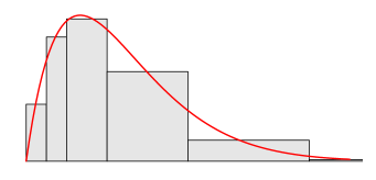
Figure 1: Density $f$ (continuous, red curve), latent distribution $\boldsymbol{\pi}$ and observed histogram (gray blocks).

Let

$$\pi_{i}=\Pr(X\in\mathcal{I}_{i})=\int_{b_{i-1}}^{b_{i}}f(t)dt=f(u_{i})\Delta+\mathcal{O}(\Delta^{2}),$$

where $\boldsymbol{\pi}=(\pi_{i})_{i=1}^{I}$ contains the values of the latent distribution on the grid of $I$ narrow intervals $\mathcal{I}_{i}$ partitioning the support of $X$. Figure 1 illustrates the construction (for a value of $\Delta$ much larger than what we use in practice). Consider a cubic B-spline basis $\{b_{k}(\cdot)\}_{k=1}^{K}$ associated to a large number of equidistant knots on $(a_{0},a_{J})$. We model the probabilities in $\boldsymbol{\pi}$ using polytomous logistic regression,

$$\pi_{i}=\pi_{i}(\boldsymbol{\theta})=\frac{\exp(\eta_{i})}{\exp(\eta_{1})+\ldots+\exp(\eta_{I})}$$ (1)

where the scores $\eta_{1},\ldots,\eta_{I}$ are connected to the B-spline basis using

$$\eta_{i}=\eta_{i}(\boldsymbol{\theta})=\sum_{k=1}^{K}b_{k}(u_{i})\theta_{k}=[\mathbf{B}\boldsymbol{\theta}]_{i}~{},$$

with each column of the matrix $[\mathbf{B}]_{ik}=b_{k}(u_{i})$ containing one of the $K$ B-splines in the basis evaluated at the small bin midpoints. In this setting, we cannot observe $\boldsymbol{\pi}$ itself, but only sums over $J<I$ intervals. The probability masses assigned to these intervals are given by

$$\Pr(X\in\mathcal{C}_{j})=\int_{a_{j-1}}^{a_{j}}f(u)du=\gamma_{j},$$

with $\gamma_{j}=\sum_{i=1}^{I}c_{ji}\pi_{i}$, or in matrix form, $\boldsymbol{\gamma}=\mathbf{C}\boldsymbol{\pi}$, where $\mathbf{C}$ is a $J\!\times I$ matrix. The likelihood based on the observed grouped data frequencies, ${{\cal D}}_{0}=\{n_{1},\ldots,n_{J}\}$, directly follows from the Multinomial distribution for the observed frequencies, $\ell(\boldsymbol{\theta}|{{\cal D}}_{0})=\sum_{j=1}^{J}n_{j}\log\gamma_{j}$. [5] proposed to put a discrete roughness penalty on the B-splines coefficients to force smoothness on the density estimate. The penalized log-likelihood based on the observed data is

$$\ell_{p}(\boldsymbol{\theta}|{{\cal D}}_{0},\lambda)=\ell(\boldsymbol{\theta}|{{\cal D}}_{0})-\frac{\lambda}{2}\|\mathbf{D}\boldsymbol{\theta}\|^{2},$$

where $\mathbf{D}$ is the $r$th order differencing matrix of size $(K-r)\!\times K$ such that $\mathbf{D}\boldsymbol{\theta}=\Delta^{r}\boldsymbol{\theta}$. For instance, with second-order differences, we have

$$\mathbf{D}=\begin{pmatrix}1&-2&1&0&\cdots&0\\ 0&\ddots&\ddots&\ddots&\ddots&\vdots\\ \vdots&\ddots&\ddots&\ddots&\ddots&0\\ 0&\cdots&0&1&-2&1\\ \end{pmatrix}.$$

3.2 Estimation from grouped frequency data using the EM algorithm

The expectation-maximization (EM) algorithm [3] is well-suited to estimate the probabilities $\boldsymbol{\pi}$ from the latent (unobserved) small bin frequencies $\mathbf{k}=(k_{1},\ldots,k_{I})$, where $n_{j}=\sum_{i}c_{ji}k_{i}$. Since $X_{1},\ldots,X_{n}$ have been assumed to be independent and identically distributed, the small bin frequencies $k_{1},\ldots,k_{I}$ are the realization of a Multinomial random vector with exponent the sample size $n$ and probability vector $\boldsymbol{\pi}$. The complete log-likelihood is then given by $\ell^{c}(\boldsymbol{\theta}|{{\cal D}}_{0}^{c})=\sum_{i=1}^{I}k_{i}\log\pi_{i}(\boldsymbol{\theta})$ where ${{\cal D}}_{0}^{c}=\{\mathbf{k}\}$. The penalized complete log-likelihood based on the complete frequency data is

$$\ell^{c}_{p}(\boldsymbol{\theta}|{{\cal D}}_{0}^{c},\lambda)=\ell^{c}(\boldsymbol{\theta}|{{\cal D}}_{0}^{c})-\frac{\lambda}{2}\|\mathbf{D}\boldsymbol{\theta}\|^{2}.$$

We propose to use Algorithm 1 to perform estimation in the described context.

Algorithm 1.

Density estimation using grouped data frequencies
The following EM algorithm alternates the update of the estimates for the latent frequencies $\mathbf{k}$, $\boldsymbol{\theta}$ and, possibly, $\lambda$ using the following steps till convergence:

1. E-step: ${k}_{i}\leftarrow\text{E}\left(k_{i}|\boldsymbol{\theta},{{\cal D}}_{0}\right)=m_{\gamma(i)}\pi_{i}({\boldsymbol{\theta}})/\gamma_{j(i)}({\boldsymbol{\theta}})$ where $j(i)$ is such that ${\cal I}_{i}\subset\mathcal{C}_{j(i)}$ ;

2. M-step: ${\boldsymbol{\theta}}=\arg\!\max_{\theta}\ell^{c}_{p}(\boldsymbol{\theta}|{{\cal D}}_{0}^{c},\lambda)$. This can be done using penalized iteratively weighted least squares (P-IWLS) or a Newton-Raphson (N-R) algorithm. Let us detail the last algorithm. Based on the following explicit forms for the gradient $\nabla_{\theta}{\ell}^{c}_{p}$ and the Hessian matrix ${\mathbf{H}_{p}^{c}}=\nabla^{2}_{\theta}{\ell}^{c}_{p}$,

   $$\nabla_{\theta}{\ell}^{c}_{p}(\boldsymbol{\theta}|{{\cal D}}_{0}^{c},\lambda)=\mathbf{B}^{\top}(\mathbf{k}-n\boldsymbol{\pi})-\lambda\mathbf{P}\boldsymbol{\theta}~{}~{};~{}-{\mathbf{H}_{p}^{c}}=-\nabla^{2}_{\theta}{\ell}^{c}_{p}(\boldsymbol{\theta}|{{\cal D}}_{0}^{c},\lambda)=\mathbf{B}^{\top}\mathbf{W}\mathbf{B}+\lambda\mathbf{P}~{},$$ (2)

   where $\mathbf{P}=\mathbf{D}^{\top}\mathbf{D}$ is the $K\!\times K$ penalty matrix and $(\mathbf{W})_{ii^{\prime}}=n(\pi_{i}\delta_{ii^{\prime}}-\pi_{i}\pi_{i^{\prime}})$, the N-R algorithm repeats, till convergence, the following substitution: $\boldsymbol{\theta}\longleftarrow\boldsymbol{\theta}+\left(-{\mathbf{H}_{p}^{c}+\epsilon\,\mathrm{I}_{K}}\right)^{-1}\nabla_{\theta}{\ell}^{c}_{p}$. The addition of a small multiple of the identity matrix to the Hessian before inversion in the N-R step is a ridge penalty that conveniently handles the identification problem in (1), as $\pi_{i}(\boldsymbol{\theta})=\pi_{i}(\boldsymbol{\theta}+c)$ for any constant $c$.

3. Penalty update: $\lambda\leftarrow({\mathrm{edf}}-r)/\|\mathbf{D}\boldsymbol{\theta}\|^{2}$ where the effective number of spline parameters is given by the trace of a matrix, ${\mathrm{edf}(\lambda)}=\operatorname{Tr}\left((-\mathbf{H}_{p}^{c}+\epsilon\,\mathrm{I}_{K})^{-1}(-\mathbf{H}_{p}^{c}-\lambda\mathbf{P})\right)$.

The last step is optional as one might prefer to perform the estimation procedure for a given value of the penalty parameter and rely on an external ad-hoc strategy to select $\lambda$. At convergence, one obtains the penalized MLE $\hat{\boldsymbol{\theta}}_{\lambda}$ (given the selected value for the penalty parameter $\lambda$). $\square$

Estimation could also be performed using the strategy described in [4] based on the composite link model [14] or in a Bayesian setting, see Section 3.3.

3.3 Estimation in a Bayesian setting

[11] suggested to estimate $f$ using the Bayesian paradigm. In that context, the roughness penalty translates into a smoothness prior for the spline coefficients,

$$p(\boldsymbol{\theta}|\lambda)\propto\lambda^{\rho(\mathbf{P})/2}\exp\left(-{\lambda\over 2}~{}{\boldsymbol{\theta}}^{\top}\mathbf{P}{\boldsymbol{\theta}}\right)$$

where $\mathbf{P}=\mathbf{D}^{\top}\mathbf{D}$ and $\rho(\mathbf{P})$ is the rank of $\mathbf{P}$. A Gamma prior ${\cal G}\left(a,b\right)$ with large variance for $\lambda$ is a possible choice to express prior ignorance about suitable values for $\lambda$, although more robust results can be obtained with a mixture of Gammas [9]. Closed forms for the joint posterior of $(\boldsymbol{\theta},\lambda)$,

$$p(\boldsymbol{\theta},\lambda|{{\cal D}}_{0})\propto\lambda^{a+\rho(\mathbf{P})/2-1}\prod_{j}\gamma_{j}^{n_{j}}\exp\left\{-\lambda(b+.5~{}{\boldsymbol{\theta}}^{\top}\mathbf{P}{\boldsymbol{\theta}})\right\}$$ (3)

and its gradient are available. The Langevin-Hastings algorithm [13] can be used to get a random sample, $\{({\boldsymbol{\theta}}^{(m)},\lambda^{(m)}),m=1,\ldots,M\}$, from the posterior. To each ${\boldsymbol{\theta}}^{(m)}$ corresponds a density $f^{(m)}$ from which any summary measure $\xi^{(m)}$ of interest such as the mean, the standard deviation or quantiles can be computed. Point estimates and credible intervals for $\xi$ can be derived from $\{\xi^{(m)}$, $m=1,\ldots,M\}$. Specific properties such as unimodality or log-concavity can be imposed on the estimated density by excluding, through the prior, the configurations of $\boldsymbol{\theta}$ corresponding to non-desirable densities. Alternatively, in that Bayesian framework, Laplace approximations can be combined in a Bayesian setting to estimate a density from grouped data in a fast and reliable way, see [[]Section 2.5] Lambert:2021. The marginal posterior for the spline parameters is very well approximated by a mixture of Normal distributions with weights defined by the marginal posterior for the log of the penalty parameter. The latter distribution can be reliably approximated by a skewed Normal distribution [6].

One can show that maximizing (3) for a given value of $\lambda$ is equivalent to maximizing $p(\boldsymbol{\theta}|\lambda,{{\cal D}}_{0})$ or the penalized complete log-likelihood $\ell^{c}_{p}(\boldsymbol{\theta}|{{\cal D}}_{0}^{c},\lambda)$. Therefore, the so-obtained conditional posterior mode coincides with the penalized MLE $\hat{\boldsymbol{\theta}}_{\lambda}$ given by the EM algorithm. Further extensions to take into account the moments observed within classes will be based on the EM algorithm.

3.4 Moment-based extensions

3.4.1 Density estimation for given class-specific sample means

Let us now further assume that, together with the frequencies $n_{j}$, the sample means $\overline{x}_{j}$ within $\mathcal{C}_{j}$ ($j=1,\ldots,J$) are also reported. Then, the likelihood based on the observed data, ${{\cal D}}_{1}={{\cal D}}_{0}\cup\{\bar{x}_{j}:j=1,\ldots,J\}$, becomes

$$L(\boldsymbol{\theta}|{{\cal D}}_{1})=\Pr\left(N_{1}=n_{1},\ldots,N_{J}=n_{J}\right)\prod_{j=1}^{J}f_{\overline{X}_{j}}(\overline{x}_{j}|n_{j})\propto\prod_{j=1}^{J}\Big{(}\gamma_{j}^{n_{j}}f_{\overline{X}_{j}}(\overline{x}_{j}|n_{j})\Big{)},$$

where $f_{\overline{X}_{j}}(\cdot|n_{j})$ is the conditional density of $\overline{X}_{j}$ given the class frequency $N_{j}=n_{j}$. Provided that the class frequency $n_{j}$ is not too small, the Central Limit theorem provides a reasonable approximation to $f_{\overline{X}_{j}}(\cdot|n_{j})$. Formally, denote the class-specific population moments as

$$\mu_{1j}={1\over\gamma_{j}}\int_{a_{j-1}}^{a_{j}}xf(x)~{}dx~{}~{}\text{and}~{}~{}\sigma^{2}_{j}={1\over\gamma_{j}}\int_{a_{j-1}}^{a_{j}}(x-\mu_{1j})^{2}f(x)dx.$$

Then,

$$f_{\overline{X}_{j}}(\overline{x}_{j}|n_{j})\approx\frac{\sqrt{n_{j}}}{\sigma_{j}\sqrt{2\pi}}\exp\left(-\frac{n_{j}}{2\sigma_{j}^{2}}(\overline{x}_{j}-\mu_{1j})^{2}\right).$$

Given the preceding spline approximation to the (log-)density using polytomous logistic regression for the probabilities to be in the small bins partitioning the support, see (1), one has

$$\mu_{1j}(\boldsymbol{\theta}) = \text{E}[X|X\in\mathcal{C}_{j}]=\sum_{i=1}^{I}u_{i}\frac{c_{ji}\pi_{i}(\boldsymbol{\theta})}{\gamma_{j}(\boldsymbol{\theta})}+\mathcal{O}(\Delta^{2}),$$

$$\sigma^{2}_{j}(\boldsymbol{\theta}) = \text{Var}[X|X\in\mathcal{C}_{j}]=\sum_{i=1}^{I}\big{(}u_{i}-\mu_{1j}(\boldsymbol{\theta})\big{)}^{2}~{}\frac{c_{ji}\pi_{i}(\boldsymbol{\theta})}{\gamma_{j}(\boldsymbol{\theta})}+\mathcal{O}(\Delta^{2}).$$

Then, for given roughness penalty parameter $\lambda$, the penalized log-likelihood based on ${{\cal D}}_{1}$ becomes

$$\ell_{p}(\boldsymbol{\theta}|{{\cal D}}_{1},\lambda)=\ell_{p}(\boldsymbol{\theta}|{{\cal D}}_{0},\lambda)-{1\over 2}\sum_{j=1}^{J}\left(\ln\sigma^{2}_{j}(\boldsymbol{\theta})+{n_{j}\over\sigma^{2}_{j}({\boldsymbol{\theta}})}\big{(}\overline{x}_{j}-\mu_{1j}(\boldsymbol{\theta})\big{)}^{2}\right),$$

while its counterpart based on latent small bins frequencies, ${{\cal D}}_{1}^{c}={{\cal D}}_{0}^{c}\cup\{\bar{x}_{j}:j=1,\ldots,J\}$, is

$$\ell_{p}^{c}(\boldsymbol{\theta}|{{\cal D}}_{1}^{c},\lambda)=\ell_{p}^{c}(\boldsymbol{\theta}|{{\cal D}}_{0}^{c},\lambda)-{1\over 2}\sum_{j=1}^{J}\left(\ln\sigma^{2}_{j}(\boldsymbol{\theta})+{n_{j}\over\sigma^{2}_{j}({\boldsymbol{\theta}})}\big{(}\overline{x}_{j}-\mu_{1j}(\boldsymbol{\theta})\big{)}^{2}\right).$$ (4)

It leads to Algorithm 2 for an estimation of the density using the EM algorithm.

Algorithm 2.

Density estimation using grouped data means and frequencies
The following EM algorithm alternates the update of the estimates for the latent frequencies $\mathbf{k}$, $\boldsymbol{\theta}$ and, possibly, $\lambda$. Denote by $\tilde{\mathbf{B}}$ the $I\!\times K$ matrix such that $(\tilde{\mathbf{B}})_{ik}=\tilde{b}_{ik}=b_{k}(u_{i})-\sum_{t=1}^{I}b_{k}(u_{t})\pi_{t}$.

Repeat the following steps till convergence:

1. E-step: ${k}_{i}\leftarrow\text{E}\left(k_{i}|\boldsymbol{\theta},{{\cal D}}_{1}\right)=m_{\gamma(i)}\pi_{i}({\boldsymbol{\theta}})/\gamma_{j(i)}({\boldsymbol{\theta}})$ where $j(i)$ is such that ${\cal I}_{i}\subset\mathcal{C}_{j(i)}$ ;

2. M-step: compute ${\boldsymbol{\theta}}=\arg\!\max_{\theta}\ell^{c}_{p}(\boldsymbol{\theta}|{{\cal D}}_{1}^{c},\lambda)$. This can be done using a Newton-Raphson (N-R) algorithm with the iterative substitution, $\boldsymbol{\theta}\longleftarrow\boldsymbol{\theta}+\left({-\mathbf{H}_{p}^{c}+\epsilon\,\mathrm{I}_{K}}\right)^{-1}\nabla_{\theta}{\ell}^{c}_{p}$, till convergence. Explicit forms for the gradient and the Hessian matrix are available after conditioning on the value $\tilde{\sigma}^{2}_{j}$ of $\sigma^{2}_{j}(\boldsymbol{\theta})$ in (4) at the start of the iteration:

   $$\begin{split}&\nabla_{\theta}{\ell}^{c}_{p}(\boldsymbol{\theta}|{{\cal D}}_{1}^{c},\lambda)=\nabla_{\theta}{\ell}^{c}_{p}(\boldsymbol{\theta}|{{\cal D}}_{0}^{c},\lambda)+\sum_{j=1}^{J}{n_{j}\over\tilde{\sigma}^{2}_{j}}\big{(}\overline{x}_{j}-\mu_{1j}\big{)}{\partial\mu_{1j}\over\partial\boldsymbol{\theta}}~{}~{};~{}\\ &-{\mathbf{H}_{p}^{c}}=-\nabla^{2}_{\theta}{\ell}^{c}_{p}(\boldsymbol{\theta}|{{\cal D}}_{1}^{c},\lambda)\approx-\nabla^{2}_{\theta}{\ell}^{c}_{p}(\boldsymbol{\theta}|{{\cal D}}_{0}^{c},\lambda)+\sum_{j=1}^{J}{n_{j}\over\tilde{\sigma}^{2}_{j}}{\partial\mu_{1j}\over\partial\boldsymbol{\theta}}{\partial\mu_{1j}\over\partial\boldsymbol{\theta}^{\top}},\end{split}$$ (5)

   where ${\partial\mu_{1j}/\partial\theta_{k}}={1\over\gamma_{j}}\sum_{i=1}^{I}c_{ji}\pi_{i}(u_{i}-\mu_{1j})b_{ik}$, with the approximation to $\mathbf{H}_{p}^{c}$ coming from the neglect of zero expectation terms.

3. Penalty update: $\lambda\leftarrow({\mathrm{edf}}-r)/\|\mathbf{D}\boldsymbol{\theta}\|^{2}$ where the effective number of spline parameters is given by the trace of a matrix, ${\mathrm{edf}(\lambda)}=\operatorname{Tr}\left((-\mathbf{H}_{p}^{c}+\epsilon\,\mathrm{I}_{K})^{-1}(-\mathbf{H}_{p}^{c}-\lambda\mathbf{P})\right)$.

At convergence, one obtains the penalized MLE $\hat{\boldsymbol{\theta}}_{\lambda}$ (given the selected value for $\lambda$). $\square$

3.4.2 Density estimation for given class-specific sample central moments

Assume now that, together with the frequencies, the sample mean $\overline{X}_{j}$, variance $S^{2}_{j}$, skewness $G_{1j}$ and kurtosis $G_{2j}$ within $\mathcal{C}_{j}$ are reported. If $M_{rj}$ denotes the $r$th sample central moment in $\mathcal{C}_{j}$, we have

$$\overline{X}_{j}=M_{1j}~{}~{};~{}~{}S^{2}_{j}=M_{2j}~{}~{};~{}~{}G_{1j}=M_{3j}/{M_{2j}^{3/2}}~{}~{};~{}~{}G_{2j}=M_{4j}/{M_{2j}^{4/2}}-3.$$

Denote by $\mathbf{M}_{j}=(M_{1j},M_{2j},M_{3j},M_{4j})$ the random vector of sample central moments in $\mathcal{C}_{j}$ and by $\mathbf{m}_{j}$ its observed counterpart. For sufficiently large values of $n_{j}$, the Central Limit theorem provides a multivariate Normal approximation to the sampling distribution of $\mathbf{M}_{j}$, $\mathbf{M}_{j}\overset{d}{\longrightarrow}\mathcal{N}_{4}\left(\boldsymbol{\mu}_{j},\Sigma_{j}\right),$ where $\boldsymbol{\mu}_{j}=(\mu_{1j},\ldots,\mu_{4j})$ with $\mu_{1j}=\mu_{j}$ and

$$\mu_{rj}=\mu_{rj}(\boldsymbol{\theta}) = \text{E}\left[(X-\mu_{1j}(\boldsymbol{\theta}))^{r}|X\in\mathcal{C}_{j}\right],\hskip 5.69054ptr=2,3,\ldots$$

$$= {1\over\gamma_{j}(\boldsymbol{\theta})}\sum_{j=1}^{J}c_{ji}\pi_{i}(\boldsymbol{\theta})\big{(}u_{i}-\mu_{1j}(\boldsymbol{\theta})\big{)}^{r}+\mathcal{O}(\Delta^{2}).$$

Using the Generalized Method of Moments (GMM) [7], one can show that

$$\Sigma_{j}={1\over n_{j}}\begin{pmatrix}\mu_{2j}&\mu_{3j}&\mu_{4j}&\mu_{5j}\\ \mu_{3j}&\mu_{4j}-\mu_{2j}^{2}&\mu_{5j}-\mu_{2j}\mu_{3j}&\mu_{6j}-\mu_{2j}\mu_{4j}\\ \mu_{4j}&\mu_{5j}-\mu_{2j}\mu_{3j}&\mu_{6j}-\mu_{3j}^{2}&\mu_{7j}-\mu_{3j}\mu_{4j}\\ \mu_{5j}&\mu_{6j}-\mu_{2j}\mu_{4j}&\mu_{7j}-\mu_{3j}\mu_{4j}&\mu_{8j}-\mu_{4j}^{2}\end{pmatrix}.$$ (6)

Based on the observed data ${{\cal D}}={{\cal D}}_{0}\cup\{\mathbf{m}_{j}:j=1,\ldots,J\}$ and for a given roughness penalty parameter $\lambda$, the penalized log-likelihood becomes

$$\ell_{p}(\boldsymbol{\theta}|{{\cal D}},\lambda)=\ell_{p}(\boldsymbol{\theta}|{{\cal D}}_{0},\lambda)-{1\over 2}\sum_{j=1}^{J}\left\{\ln|\Sigma_{j}|+(\mathbf{m}_{j}-\boldsymbol{\mu}_{j})^{\top}\Sigma_{j}^{-1}(\mathbf{m}_{j}-\boldsymbol{\mu}_{j})\right\},$$ (7)

comparable to (4) when only the tabulated sample means were available. When, in addition, the latent small bins frequencies are given, ${{\cal D}}^{c}={{\cal D}}^{c}_{0}\cup\{\mathbf{m}_{j}:j=1,\ldots,J\}$, inference is based on the penalized complete log-likelihood,

$$\ell^{c}_{p}(\boldsymbol{\theta}|{{\cal D}}^{c},\lambda)=\ell^{c}_{p}(\boldsymbol{\theta}|{{\cal D}}^{c}_{0},\lambda)-{1\over 2}\sum_{j=1}^{J}\left\{\ln|\Sigma_{j}|+(\mathbf{m}_{j}-\boldsymbol{\mu}_{j})^{\top}\Sigma_{j}^{-1}(\mathbf{m}_{j}-\boldsymbol{\mu}_{j})\right\}.$$ (8)

The maximization of the penalized log-likelihood (7) and the selection of $\lambda$ can be made using Algorithm 3.

Algorithm 3.

Density estimation given class-specific sample moments and frequencies
The following EM algorithm alternates the update of the estimates for the latent frequencies $\mathbf{k}$, $\boldsymbol{\theta}$ and, possibly, $\lambda$ using the following steps till convergence:

1. E-step: ${k}_{i}\leftarrow\text{E}\left(k_{i}|\boldsymbol{\theta},{{\cal D}}_{1}\right)=m_{\gamma(i)}\pi_{i}({\boldsymbol{\theta}})/\gamma_{j(i)}({\boldsymbol{\theta}})$ where $j(i)$ is such that ${\cal I}_{i}\subset\mathcal{C}_{j(i)}$ ;

2. M-step: compute ${\boldsymbol{\theta}}=\arg\!\max_{\theta}\ell^{c}_{p}(\boldsymbol{\theta}|{{\cal D}}^{c},\lambda)$. This can be done using a Newton-Raphson (N-R) algorithm with the iterative substitution, $\boldsymbol{\theta}\longleftarrow\boldsymbol{\theta}+\left({-\mathbf{H}_{p}^{c}+\epsilon\,\mathrm{I}_{K}}\right)^{-1}\nabla_{\theta}{\ell}^{c}_{p}$, till convergence. Explicit forms for the gradient and the Hessian matrix are available after conditioning on the value $\tilde{\Sigma}_{j}$ of $\Sigma_{j}(\boldsymbol{\theta})$ in (8) at the start of the iteration:

   $$\begin{split}\big{(}\nabla_{\theta}{\ell}^{c}_{p}\big{)}_{k}&=\big{(}\nabla_{\theta}{\ell}^{c}_{p}(\boldsymbol{\theta}|{{\cal D}}_{0}^{c},\lambda)\big{)}_{k}+\sum_{j=1}^{J}(\mathbf{m}_{j}-\boldsymbol{\mu}_{j})^{\top}\tilde{\Sigma}_{j}^{-1}{\partial\boldsymbol{\mu}_{j}\over\partial\theta_{k}}~{}~{};~{}\\ -\big{(}{\mathbf{H}_{p}^{c}}\big{)}_{ks}&\approx-\big{(}\nabla^{2}_{\theta}{\ell}^{c}_{p}(\boldsymbol{\theta}|{{\cal D}}_{0}^{c},\lambda)\big{)}_{ks}+\sum_{j=1}^{J}{\partial\boldsymbol{\mu}^{\top}_{j}\over\partial\theta_{s}}\tilde{\Sigma}_{j}^{-1}{\partial\boldsymbol{\mu}_{j}\over\partial\theta_{k}}\end{split}$$ (9)

   with

   $${\partial\mu_{rj}\over\partial\theta_{k}} ={1\over\gamma_{j}}\sum_{i=1}^{I}c_{ji}\pi_{i}b_{ik}\big{\{}(u_{i}-\mu_{1j})^{r}-\mu_{rj}\big{\}}-r\mu_{r-1,j}{\partial\mu_{1j}\over\partial\theta_{k}}$$

   $$={1\over\gamma_{j}}\sum_{i=1}^{I}c_{ji}\pi_{i}b_{ik}\big{\{}(u_{i}-\mu_{1j})^{r}-\mu_{rj}-r\mu_{r-1,j}(u_{i}-\mu_{1j})\big{\}}$$ (10)

   for $1\leq k,s\leq K$ and $2\leq r\leq 4$.

3. Penalty update: $\lambda\leftarrow({\mathrm{edf}}-r)/\|\mathbf{D}\boldsymbol{\theta}\|^{2}$ where the effective number of spline parameters is given by the trace of a matrix, ${\mathrm{edf}(\lambda)}=\operatorname{Tr}\left((-\mathbf{H}_{p}^{c}+\epsilon\,\mathrm{I}_{K})^{-1}(-\mathbf{H}_{p}^{c}-\lambda\mathbf{P})\right)$.

At convergence, one obtains the penalized MLE $\hat{\boldsymbol{\theta}}_{\lambda}$ (given the selected value for $\lambda$). $\square$

3.5 Quantile estimation

Consider the following shorthand notation for the conditional posterior mode of the vector of spline parameters underlying the density estimate, ${\hat{\boldsymbol{\theta}}}={\hat{\boldsymbol{\theta}}}_{\lambda}-\max\{\hat{\theta}_{k}\}_{k=1}^{K}$, with a substraction of the largest estimated component to handle the identification issue following from $\boldsymbol{\pi}(\boldsymbol{\theta}+c)=\boldsymbol{\pi}(\boldsymbol{\theta})$ for any real number $c$. Denote by $\hat{k}$ the component for which $(\hat{\boldsymbol{\theta}})_{\hat{k}}=0$ and by $\boldsymbol{\theta}_{-\hat{k}}$ the vector of spline parameters where the $\hat{k}$th component of $\boldsymbol{\theta}$ is omitted. Quantile estimates can be derived using the fitted density estimate,

$$f(x|\hat{\boldsymbol{\theta}})={\exp\{\eta(x|\hat{\boldsymbol{\theta}})\}/\int_{\cal X}\exp\{\eta(t|\hat{\boldsymbol{\theta}})\}\,dt}\,,$$

where $\eta(x|{\boldsymbol{\theta}})=\sum_{k=1}^{K}b_{k}(x)\theta_{k}$ and ${\cal X}=(a_{0},a_{J})$ denotes the support of the density. Indeed, as the associated estimate for the cumulative distribution function (CDF), $\hat{F}(x)=F(x|\hat{\boldsymbol{\theta}})=\int_{a_{0}}^{x}f(t|\hat{\boldsymbol{\theta}})\,dt$, is monotone, it can be inverted to provide an estimate of the quantile function,

$$\hat{Q}(p)=Q(p|\hat{\boldsymbol{\theta}})=\inf\{x\in{\rm I\!R}:F(x|\hat{\boldsymbol{\theta}})\geq p\}.$$

Practically, starting for the fitted probability, $\hat{\pi}_{i}=\Pr(X\in\mathcal{I}_{i}|\hat{\boldsymbol{\theta}})$, to have an observation in the small bin $\mathcal{I}_{i}=(b_{i-1},b_{i}]$ ($i=1,\ldots,I$), see Section 3.1, and with $\hat{F}(b_{0})=0$, $\hat{F}(b_{i})=\hat{\pi}_{1}+\ldots+\hat{\pi}_{i}$, a first guess for $\hat{Q}(p)$ is given by

$$x_{0}=\max_{0\leq i\leq I}\big{\{}b_{i}:\hat{F}(b_{i})\leq p\big{\}}\,.$$

This first approximation can be improved in an iterative way with, at iteration $t$,

$$x_{t}\longleftarrow x_{t-1}+\big{(}p-F(x_{t-1}|\hat{\boldsymbol{\theta}})\big{)}/f(x_{t-1}|\hat{\boldsymbol{\theta}})\,,$$

yielding at convergence $Q(p|\hat{\boldsymbol{\theta}})=x_{\infty}$. The uncertainty in that estimation directly follows from the uncertainty in the choice of $\boldsymbol{\theta}$. The latter is quantified by the conditional posterior distribution of ${\boldsymbol{\theta}}_{-\hat{k}}$ with Laplace approximation $\big{(}{\boldsymbol{\theta}}_{-\hat{k}}|{{\cal D}},\lambda\big{)}\stackrel{{\scriptstyle\cdot}}{{\sim}}{\cal N}\big{(}{\hat{{\boldsymbol{\theta}}}}_{-\hat{k}},({\cal J}_{-\hat{k},-\hat{k}})^{-1}\big{)}$ where

$${\cal J}_{ks} =-\big{(}\nabla^{2}_{{\theta}}{\ell}_{p}(\boldsymbol{\theta}|{{\cal D}}_{0},\lambda)\big{)}_{ks}+\sum_{j=1}^{J}{\partial\boldsymbol{\mu}^{\top}_{j}\over\partial\theta_{s}}\tilde{\Sigma}_{j}^{-1}{\partial\boldsymbol{\mu}_{j}\over\partial\theta_{k}}\,,$$ (11)

with the partial derivatives of the theoretical central moments $\boldsymbol{\mu}_{j}$ in the $j$th class given in (10). The second derivatives of the log-likelihood based on the observed class frequencies ${{\cal D}}_{0}$ in the first term of (11) has an explicit form given by

$$-\big{(}\nabla^{2}_{\theta}{\ell}_{p}(\boldsymbol{\theta}|{{\cal D}}_{0},\lambda)\big{)}_{ks} =n\sum_{i=1}^{I}b_{ik}\pi_{i}\tilde{b}_{is}+\sum_{j=1}^{J}{n_{j}\over\gamma_{j}{{}^{2}}}\sum_{\ell=1}^{I}c_{j\ell}\pi_{\ell}\tilde{b}_{\ell s}\sum_{i=1}^{I}c_{ji}\pi_{i}\tilde{b}_{ik}-\sum_{j=1}^{J}{n_{j}\over\gamma_{j}}\sum_{i=1}^{I}c_{ji}\pi_{i}\tilde{b}_{is}\tilde{b}_{ik}$$

$$=(\mathbf{B}^{\top}\mathbf{W}\mathbf{B})_{ks}-\sum_{j=1}^{J}{n_{j}\over\gamma_{j}}\sum_{i=1}^{I}c_{ji}\pi_{i}{b}_{ik}\left(b_{is}-{1\over\gamma_{j}}\sum_{\ell=1}^{I}c_{j\ell}\pi_{\ell}b_{\ell s}\right).$$

The first term in the last expression, where $(\mathbf{W})_{ii^{\prime}}=n(\pi_{i}\delta_{ii^{\prime}}-\pi_{i}\pi_{i^{\prime}})$, corresponds to the information available on $\boldsymbol{\theta}$ based on data frequencies in the absence of class tabulation. The information reduction due to tabulation is quantified by the second term. Based on the following first-order expansion,

$$Q(p|\boldsymbol{\theta})\approx Q(p|\hat{\boldsymbol{\theta}})+{\partial Q(p|\hat{\boldsymbol{\theta}})\over\partial\boldsymbol{\theta}_{-\hat{k}}^{\top}}(\boldsymbol{\theta}-\hat{\boldsymbol{\theta}})_{-\hat{k}}\,,$$

the conditional posterior distribution of $Q(p|\boldsymbol{\theta})$ can be approximated by

$$\big{(}Q(p|\boldsymbol{\theta})|{{\cal D}},\lambda\big{)}\stackrel{{\scriptstyle\cdot}}{{\sim}}{\cal N}\left(Q(p|\hat{\boldsymbol{\theta}}),s^{2}_{Q}(p)\right)\,,$$ (12)

with

$${\partial Q(p|\hat{\boldsymbol{\theta}})\over\partial\theta_{k}} ={1\over f\big{(}Q(p|\hat{\boldsymbol{\theta}})|\hat{\boldsymbol{\theta}}\big{)}}\left\{\int_{-\infty}^{Q(p|\hat{\boldsymbol{\theta}})}b_{k}(x)f(x|\hat{\boldsymbol{\theta}})\,dx-p\int_{\rm I\!R}b_{k}(x)f(x|\hat{\boldsymbol{\theta}})\,dx\right\}\,,$$

$$s^{2}_{Q}(p) ={\partial Q(p|\hat{\boldsymbol{\theta}})\over\partial\boldsymbol{\theta}_{-\hat{k}}^{\top}}\,({\cal J}_{-\hat{k},-\hat{k}})^{-1}\,{\partial Q(p|\hat{\boldsymbol{\theta}})\over\partial\boldsymbol{\theta}_{-\hat{k}}}\,.$$

Therefore, an approximate $100(1-\alpha)\%$ credible interval for $Q(p)$ is given by

$$Q(p|\hat{\boldsymbol{\theta}})\pm\Phi^{-1}(1-\alpha/2)\,s_{Q}(p)\,,$$ (13)

with $\Phi^{-1}(\cdot)$ denoting the quantile function of the standard Normal distribution.

4 Simulation study

In this section, we evaluate the performances of the estimation method proposed in Section 3 by means of extensive simulations. Independent and identically distributed data were generated from a mixture density,

$$f(x)=w_{1}f_{1}(x)+w_{2}f_{2}(5.6-x)$$

where $f_{1}(\cdot)$ corresponds to a Normal density with mean $1.0$ and variance $9.0^{-1}$, $f_{2}(\cdot)$ to a Gamma density with mean $11/6$ and variance $11/6^{2}$, weighted respectively by $w_{1}=.20$ and $w_{2}=.80$. It corresponds to the solid red curve in Figs. 2 and 3 that could be viewed as the underlying distribution of log transformed positive data. Datasets of size $n=250$, $1\,000$ or $3\,000$ were generated $S=500$ times and grouped into either $J=3$ or $J=5$ partitioning classes $\{{\cal C}_{j}:j=1,\ldots,J\}$ with interval extremities given by $\{-1.0,1.0,3.5,6.0\}$ and $\{-1.0,1.0,2.2,3.5,4.8,6.0\}$, respectively. Tabulated frequencies $(n_{j})_{J=1}^{J}$ and the associated local central moments $(m_{rj})_{j=1}^{J}$ of order $r=1$ up to $4$ were computed and used with the methodology of Section 3 to produce an estimate $\hat{f}(\cdot|{\cal D}_{r})$ of the underlying density on $(-1.0,6.0)$, with ${\cal D}_{r}=\bigcup_{j=1}^{J}\{n_{j},m_{1j},\ldots,m_{rj}\}$ denoting the available data. Selected quantile estimates $\hat{Q}(p|{\cal D}_{r})$ were computed using that density and compared to the ‘true’ quantile values associated to $f(\cdot)$. Biases, standard deviations (SD), root mean squared errors (RMSE) and effective coverages of 95% and 90% credible intervals are given in Tables 1, 2 and 3 for different samples sizes and number of classes. As expected, biases for the point estimator of a given quantile tend to decrease with the sample size and the number of classes for which tabulated summary statistics are observed. They are already very small when $n=250$ with $r=4$ moments reported in only $J=3$ classes, see Fig. 3 for a graphical illustration at the density level when $n=250$ and $n=1000$. An exception concerns the 20% quantile ($=1.793$) that is not so well estimated whatever the simulation setting: it corresponds to the region surrounding the local minimum of the mixture density between the two modes. Increasing the number of reported central moments tends to improve the estimation of density and quantiles, with 4 moments being preferable, see Fig. 2 for an evolution of the averaged density estimates (over the $S=500$ replicates) starting with ${{{\cal D}}_{1}}$ (dotted curve) to ${{\cal D}}_{4}$ (dashed curve) when $n=1\,000$. This is a remarkable improvement over the estimate that would be obtained using only observed frequencies. Whatever the sample size, the effective coverages of 90% and 95% credible intervals for the reported quantiles (except the 20% one) are in agreement with their nominal values when 4 central moments (${{\cal D}}_{4}$) are reported. Moderate undercoverages can be observed with ${{\cal D}}_{2}$, while the effective coverages can be larger than expected when just the means are reported in addition to frequencies (${{\cal D}}_{1}$). Global metrics were also calculated to compare the true and estimated quantile functions,

$$\ell_{1}(Q,\hat{Q})=\int_{0}^{1}\big{|}Q(p|\hat{\boldsymbol{\theta}})-Q(p)\big{|}\,dp\,$$

as well the true and estimated densities,

$$\text{RIMSE}(f,\hat{f}) =\int_{\rm I\!R}\big{(}f(x|\hat{\boldsymbol{\theta}})-f(x)\big{)}^{2}\,f(x)\,dx~{}~{};$$

$$\text{KL}(f,\hat{f}) =\int_{\rm I\!R}f(x)\log\left({f(x)\over\hat{f}(x)}\right)\,dx~{},$$

see Table 4 for their median values over the $S=500$ simulated datasets with tabulated summary statistics ${{\cal D}}_{r}$ ($r=1,2,4$) in 3 or 5 classes. This suggests that the extra information provided by additional central moments for quantile or density estimation is even more valuable when the number of classes is small.

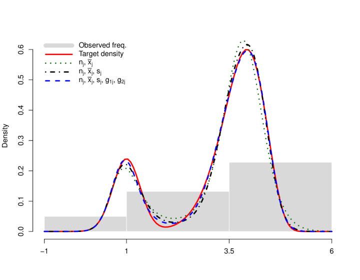
Figure 2: Simulation study ($n=1000$, $J=3$) – Density estimates from tabulated summary statistics ${{\cal D}}_{1}$ (dotted), ${{\cal D}}_{2}$ (dot-dashed) and ${{\cal D}}_{4}$ (dashed) averaged over the $S=500$ replicates, with the ’true’ underlying density (solid curve).

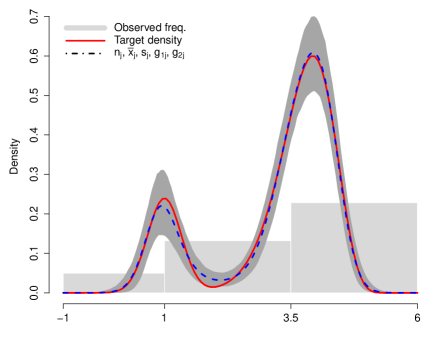
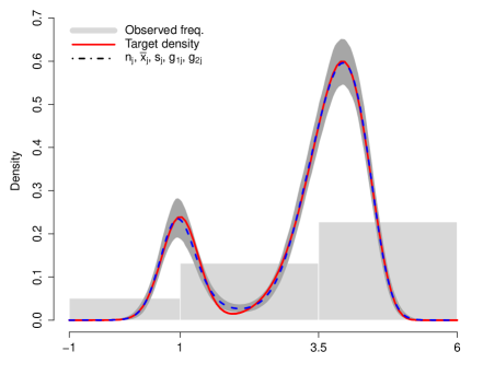
Figure 3: Simulation study – Connected pointwise intervals containing 95% of the estimated densities over the $S=500$ datasets and obtained using tabulated summary statistics ${\cal D}_{4}$ over $J=3$ classes. Left panel: $n=250$ ; Right panel: $n=1\,000$.

$p$	0.1	0.2	0.3	0.4	0.5	0.6	0.7	0.8	0.9
$Q(p)$	1.000	1.793	3.122	3.430	3.643	3.822	3.989	4.163	4.375
$J=3$ (classes)
$\hat{Q}(p|{\cal D}_{1})$	1.084	2.071	3.081	3.421	3.630	3.801	3.965	4.144	4.383
Bias	0.084	0.278	-0.041	-0.009	-0.014	-0.021	-0.024	-0.019	0.007
SD	0.121	0.401	0.154	0.074	0.054	0.045	0.040	0.038	0.048
RMSE	0.147	0.488	0.160	0.075	0.056	0.050	0.046	0.043	0.049
95% CI	0.950	0.694	0.930	0.964	0.958	0.964	0.968	0.934	0.926
90% CI	0.904	0.622	0.880	0.922	0.924	0.926	0.920	0.870	0.866
$\hat{Q}(p|{\cal D}_{2})$	1.016	2.003	3.166	3.466	3.663	3.830	3.988	4.155	4.363
Bias	0.016	0.210	0.045	0.036	0.020	0.008	-0.001	-0.009	-0.013
SD	0.082	0.493	0.124	0.064	0.050	0.044	0.040	0.039	0.040
RMSE	0.084	0.536	0.132	0.073	0.054	0.044	0.040	0.040	0.042
95% CI	0.950	0.656	0.860	0.886	0.908	0.932	0.934	0.896	0.840
90% CI	0.906	0.586	0.778	0.830	0.842	0.878	0.876	0.848	0.762
$\hat{Q}(p|{\cal D}_{4})$	1.007	2.004	3.121	3.435	3.646	3.823	3.988	4.160	4.369
Bias	0.007	0.211	-0.001	0.005	0.003	0.001	-0.001	-0.004	-0.006
SD	0.081	0.480	0.121	0.068	0.053	0.046	0.041	0.040	0.041
RMSE	0.082	0.525	0.121	0.068	0.054	0.046	0.041	0.040	0.041
95% CI	0.948	0.740	0.946	0.954	0.950	0.948	0.962	0.950	0.948
90% CI	0.910	0.694	0.918	0.912	0.908	0.912	0.924	0.904	0.880
$J=5$ (classes)
$\hat{Q}(p|{\cal D}_{1})$	0.986	1.920	3.104	3.429	3.648	3.827	3.992	4.159	4.364
Bias	-0.014	0.127	-0.018	-0.001	0.005	0.006	0.002	-0.004	-0.011
SD	0.081	0.532	0.129	0.074	0.057	0.048	0.042	0.041	0.044
RMSE	0.082	0.547	0.131	0.074	0.058	0.048	0.043	0.042	0.046
95% CI	0.910	0.650	0.938	0.930	0.936	0.932	0.912	0.882	0.898
90% CI	0.866	0.598	0.900	0.894	0.892	0.892	0.864	0.818	0.838
$\hat{Q}(p|{\cal D}_{2})$	0.998	1.914	3.100	3.423	3.640	3.820	3.988	4.162	4.373
Bias	-0.002	0.121	-0.022	-0.007	-0.003	-0.002	-0.001	-0.002	-0.002
SD	0.081	0.532	0.132	0.073	0.056	0.048	0.043	0.043	0.047
RMSE	0.081	0.545	0.134	0.073	0.056	0.048	0.043	0.043	0.047
95% CI	0.920	0.608	0.948	0.934	0.934	0.924	0.910	0.842	0.732
90% CI	0.878	0.548	0.904	0.880	0.884	0.878	0.860	0.792	0.654
$\hat{Q}(p|{\cal D}_{4})$	1.012	2.001	3.120	3.435	3.646	3.822	3.987	4.157	4.368
Bias	0.012	0.208	-0.002	0.005	0.002	0.000	-0.003	-0.006	-0.008
SD	0.091	0.480	0.120	0.068	0.054	0.046	0.041	0.039	0.040
RMSE	0.092	0.523	0.120	0.068	0.054	0.046	0.041	0.040	0.041
95% CI	0.952	0.728	0.946	0.952	0.950	0.948	0.960	0.952	0.940
90% CI	0.914	0.680	0.928	0.906	0.910	0.906	0.922	0.910	0.874

Table 1: Simulation study ($n=250$) – Selected $p-$quantile estimates using tabulated summary statistics in ${\cal D}_{r}$ with $r=1,2,4$: bias, standard deviation, root mean squared error (RMSE) and effective coverages of 95% and 90% credible intervals (based on $S=500$ replicates).

$p$	0.1	0.2	0.3	0.4	0.5	0.6	0.7	0.8	0.9	0.95
$Q(p)$	1.000	1.793	3.122	3.430	3.643	3.822	3.989	4.163	4.375	4.530
$J=3$ (classes)
$\hat{Q}(p|{\cal D}_{1})$	1.026	1.940	3.121	3.436	3.634	3.800	3.960	4.138	4.381	4.586
Bias	0.027	0.147	-0.001	0.005	-0.009	-0.022	-0.029	-0.025	0.006	0.056
SD	0.047	0.257	0.069	0.037	0.028	0.024	0.021	0.020	0.025	0.033
RMSE	0.054	0.297	0.069	0.037	0.030	0.032	0.036	0.032	0.025	0.065
95% CI	0.944	0.836	0.954	0.930	0.954	0.972	0.980	0.948	0.960	0.998
90% CI	0.878	0.786	0.910	0.894	0.916	0.920	0.920	0.892	0.918	0.978
$\hat{Q}(p|{\cal D}_{2})$	1.005	1.867	3.159	3.452	3.653	3.826	3.989	4.159	4.369	4.527
Bias	0.006	0.074	0.037	0.022	0.010	0.004	0.000	-0.005	-0.007	-0.003
SD	0.040	0.302	0.058	0.035	0.028	0.025	0.023	0.021	0.021	0.023
RMSE	0.040	0.311	0.068	0.042	0.030	0.025	0.023	0.022	0.022	0.023
95% CI	0.960	0.752	0.834	0.880	0.918	0.916	0.910	0.886	0.874	0.816
90% CI	0.902	0.698	0.768	0.812	0.844	0.866	0.844	0.820	0.788	0.728
$\hat{Q}(p|{\cal D}_{4})$	0.993	1.904	3.125	3.429	3.642	3.822	3.991	4.165	4.376	4.530
Bias	-0.006	0.111	0.003	-0.001	-0.001	0.000	0.002	0.002	0.001	0.001
SD	0.037	0.331	0.058	0.037	0.029	0.025	0.023	0.021	0.021	0.023
RMSE	0.037	0.349	0.058	0.037	0.029	0.025	0.023	0.022	0.021	0.023
95% CI	0.950	0.816	0.938	0.942	0.940	0.946	0.948	0.956	0.952	0.958
90% CI	0.904	0.776	0.892	0.898	0.890	0.904	0.898	0.896	0.904	0.908
$J=5$ (classes)
$\hat{Q}(p|{\cal D}_{1})$	0.989	1.864	3.108	3.427	3.648	3.828	3.992	4.161	4.367	4.522
Bias	-0.010	0.071	-0.014	-0.003	0.005	0.006	0.003	-0.003	-0.009	-0.008
SD	0.034	0.370	0.061	0.039	0.032	0.026	0.023	0.022	0.023	0.025
RMSE	0.036	0.377	0.063	0.040	0.032	0.027	0.023	0.022	0.024	0.027
95% CI	0.950	0.734	0.920	0.928	0.936	0.930	0.916	0.858	0.934	0.966
90% CI	0.900	0.686	0.848	0.894	0.884	0.880	0.830	0.786	0.882	0.928
$\hat{Q}(p|{\cal D}_{2})$	0.992	1.836	3.106	3.426	3.642	3.821	3.989	4.164	4.378	4.536
Bias	-0.008	0.043	-0.016	-0.004	-0.001	-0.001	-0.001	0.001	0.003	0.006
SD	0.036	0.357	0.064	0.038	0.030	0.026	0.024	0.023	0.024	0.026
RMSE	0.037	0.360	0.066	0.038	0.030	0.026	0.024	0.023	0.024	0.026
95% CI	0.942	0.730	0.912	0.938	0.932	0.924	0.890	0.816	0.692	0.808
90% CI	0.874	0.690	0.842	0.890	0.892	0.866	0.820	0.744	0.592	0.734
$\hat{Q}(p|{\cal D}_{4})$	0.995	1.914	3.121	3.429	3.643	3.823	3.990	4.164	4.374	4.530
Bias	-0.005	0.121	-0.001	-0.001	0.000	0.001	0.001	0.000	-0.002	0.000
SD	0.037	0.342	0.059	0.037	0.029	0.025	0.023	0.022	0.022	0.023
RMSE	0.037	0.363	0.059	0.037	0.029	0.025	0.023	0.022	0.022	0.023
95% CI	0.954	0.804	0.936	0.942	0.940	0.940	0.946	0.956	0.944	0.956
90% CI	0.910	0.754	0.890	0.900	0.896	0.904	0.900	0.880	0.892	0.914

Table 2: Simulation study ($n=1000$) – Selected $p-$quantile estimates using tabulated summary statistics in ${\cal D}_{r}$ with $r=1,2,4$: bias, standard deviation, root mean squared error (RMSE) and effective coverages of 95% and 90% credible intervals (based on $S=500$ replicates).

$p$	0.1	0.2	0.3	0.4	0.5	0.6	0.7	0.8	0.9	0.95	0.99
$Q(p)$	1.000	1.793	3.122	3.430	3.643	3.822	3.989	4.163	4.375	4.530	4.778
$J=3$ (classes)
$\hat{Q}(p|{\cal D}_{1})$	1.013	1.897	3.127	3.438	3.634	3.796	3.954	4.131	4.376	4.591	5.052
Bias	0.013	0.104	0.005	0.008	-0.010	-0.025	-0.035	-0.033	0.000	0.061	0.274
SD	0.025	0.145	0.038	0.021	0.016	0.013	0.011	0.010	0.013	0.020	0.045
RMSE	0.029	0.179	0.038	0.023	0.019	0.029	0.037	0.034	0.013	0.064	0.278
95% CI	0.948	0.934	0.990	0.928	0.960	0.992	0.996	0.994	0.996	1.000	1.000
90% CI	0.886	0.874	0.972	0.866	0.916	0.944	0.974	0.968	0.996	0.996	1.000
$\hat{Q}(p|{\cal D}_{2})$	1.004	1.810	3.153	3.444	3.649	3.825	3.990	4.160	4.368	4.524	4.797
Bias	0.005	0.017	0.032	0.014	0.005	0.003	0.001	-0.003	-0.007	-0.006	0.019
SD	0.023	0.170	0.032	0.021	0.017	0.014	0.013	0.012	0.011	0.012	0.021
RMSE	0.023	0.171	0.045	0.025	0.018	0.014	0.013	0.013	0.014	0.013	0.028
95% CI	0.954	0.828	0.762	0.868	0.936	0.942	0.904	0.932	0.886	0.818	0.942
90% CI	0.910	0.762	0.686	0.794	0.866	0.876	0.840	0.832	0.810	0.750	0.866
$\hat{Q}(p|{\cal D}_{4})$	0.994	1.868	3.126	3.429	3.643	3.822	3.991	4.165	4.376	4.528	4.782
Bias	-0.006	0.075	0.004	-0.001	-0.000	0.001	0.001	0.002	0.000	-0.002	0.004
SD	0.021	0.223	0.033	0.021	0.017	0.014	0.013	0.012	0.012	0.012	0.018
RMSE	0.022	0.235	0.033	0.022	0.017	0.014	0.013	0.012	0.012	0.013	0.018
95% CI	0.948	0.904	0.946	0.948	0.956	0.956	0.954	0.946	0.966	0.964	0.968
90% CI	0.902	0.850	0.894	0.880	0.894	0.914	0.906	0.910	0.914	0.918	0.918
$J=5$ (classes)
$\hat{Q}(p|{\cal D}_{1})$	0.999	1.864	3.115	3.430	3.644	3.820	3.986	4.161	4.376	4.530	4.771
Bias	-0.001	0.071	-0.007	0.000	0.001	-0.002	-0.004	-0.002	0.001	0.000	-0.007
SD	0.020	0.258	0.034	0.023	0.018	0.015	0.014	0.013	0.017	0.019	0.019
RMSE	0.020	0.268	0.035	0.023	0.018	0.015	0.014	0.013	0.017	0.019	0.020
95% CI	0.958	0.846	0.944	0.952	0.976	0.982	0.938	0.908	0.974	0.976	0.984
90% CI	0.920	0.772	0.882	0.880	0.922	0.946	0.858	0.826	0.926	0.932	0.934
$\hat{Q}(p|{\cal D}_{2})$	0.997	1.831	3.114	3.433	3.646	3.822	3.987	4.161	4.375	4.530	4.777
Bias	-0.003	0.038	-0.008	0.003	0.003	0.000	-0.002	-0.002	-0.001	0.000	-0.001
SD	0.021	0.252	0.035	0.022	0.017	0.014	0.013	0.013	0.013	0.013	0.018
RMSE	0.022	0.255	0.036	0.022	0.017	0.014	0.014	0.013	0.013	0.013	0.018
95% CI	0.942	0.814	0.934	0.932	0.938	0.910	0.896	0.852	0.746	0.894	0.972
90% CI	0.902	0.750	0.860	0.882	0.876	0.858	0.800	0.788	0.668	0.824	0.924
$\hat{Q}(p|{\cal D}_{4})$	0.996	1.875	3.123	3.430	3.644	3.823	3.990	4.164	4.375	4.527	4.778
Bias	-0.004	0.082	0.001	0.000	0.000	0.001	0.001	0.001	-0.001	-0.003	0.000
SD	0.021	0.241	0.033	0.021	0.017	0.014	0.013	0.012	0.012	0.013	0.016
RMSE	0.021	0.255	0.033	0.021	0.017	0.014	0.013	0.012	0.012	0.013	0.016
95% CI	0.958	0.860	0.958	0.946	0.954	0.960	0.948	0.942	0.962	0.958	0.982
90% CI	0.902	0.820	0.896	0.884	0.892	0.910	0.904	0.904	0.904	0.928	0.952

Table 3: Simulation study ($n=3000$) – Selected $p-$quantile estimates using tabulated summary statistics in ${\cal D}_{r}$ with $r=1,2,4$: bias, standard deviation, root mean squared error (RMSE) and effective coverages of 95% and 90% credible intervals (based on $S=500$ replicates).

		$J=3$ (classes)				$J=5$ (classes)
$n$	Metric	${\cal D}_{1}$	${\cal D}_{2}$	${\cal D}_{4}$		${\cal D}_{1}$	${\cal D}_{2}$	${\cal D}_{4}$
$250$	$\ell_{1}(Q,\hat{Q})$	0.087	0.072	0.067		0.072	0.071	0.068
	RIMSE	0.048	0.044	0.037		0.043	0.043	0.037
	K-L	0.034	0.022	0.016		0.018	0.019	0.016
$1\,000$	$\ell_{1}(Q,\hat{Q})$	0.051	0.038	0.034		0.037	0.036	0.034
	RIMSE	0.041	0.025	0.020		0.025	0.024	0.020
	K-L	0.025	0.011	0.006		0.006	0.006	0.005
$3\,000$	$\ell_{1}(Q,\hat{Q})$	0.044	0.025	0.021		0.023	0.021	0.021
	RIMSE	0.044	0.018	0.014		0.018	0.016	0.013
	K-L	0.026	0.008	0.003		0.003	0.002	0.002

Table 4: Simulation study – $L_{1}-$distance, $\ell_{1}(Q,\hat{Q})$, between the true and the estimated quantile functions ; Root integrated mean squared error (RIMSE) and Kullback-Liebler divergence (K-L) comparing the true and estimated density functions. Median values of these metrics (over $S=500$ simulated datasets of size $n$) are reported with estimation performed from tabulated summary statistics ${\cal D}_{r}$ (with $r=1,2,4$) in $J$ classes.

In summary, this simulation study confirms the added value of central moments over isolated frequencies for density estimation. With only 15 numbers (the frequency and the 4 central moments in each of the $J=3$ classes), an accurate and precise density estimate could be obtained from summary statistics in just $3$ classes, see Fig. 3 for a graphical representation. The simulation study also suggests that this method can be used to estimate quantiles and, consequently, values at risk (VaR) in a reliable way.

5 Application

Table 5 provides summary statistics on insurance claim amount data (in euros). For confidentiality reasons, the 3 518 data were rescaled and gathered in $J=3$ classes of increasing width. Besides the class frequencies $n_{j}$, the sample mean, standard deviation, skewness and kurtosis of the $\log_{10}$ transformed claims within each class are also provided.

		$\log_{10}$(Claim)
Claim	Freq.	Interval	Mean	Std.dev	Skewness	Kurtosis
Interval	$n_{j}$	$\mathcal{C}_{j}$	$\overline{x}_{j}$	$s_{j}$	$g_{1j}$	$g_{2j}$
(1 ; 1 000]	1168	(0.00 ; 3.00]	2.462	0.580	$-1.793$	$2.401$
(1 000 ; 20 000]	2234	(3.00 ; 4.30]	3.529	0.336	$0.375$	$-0.836$
(20 000 ; 1 500 000]	116	(4.30 ; 6.18]	4.556	0.275	$2.603$	$9.416$

Table 5: Car insurance data: summary statistics for $n=3518$ grouped claim data (in euros).

Figure 4 displays the histogram corresponding to the grouped data frequencies. The thick solid (red) line corresponds to the ’target’ density estimated from the precise individual ($\log_{10}$) claims shared with us in confidentiality by the insurance company. Estimation of the density using the grouped summary statistics in Table 5 was performed using the methods described in Sections 3.2 and 3.4 with $K=25$ B-splines associated to equidistant knots on $(0.0,6.18)$. Computation was performed in less than one second using the R-package degross (Density Estimation from GRouped Summary Statistics) developed and maintained by the author. The top graph in the figure compares the ’target’ density with the density estimates obtained from the grouped data frequencies (${{\cal D}}_{0}$, dotted line) and from the addition of the grouped sample means (${{\cal D}}_{1}$, dashed line). The bottom graph further considers the cumulative addition of the grouped sample standard deviations (${{\cal D}}_{2}$, dotted line), skewness and kurtosis (${{\cal D}}_{4}$, dashed line) to perform density estimation. An important improvement is observed with the addition of the standard deviations in the dataset. This is confirmed numerically by inspecting the evolution of the root integrated mean squared error (RIMSE) and of the Kullback-Leibler (K-L) divergence between the ’target’ density and the estimate obtained using sample moments of increasing orders, see Table 6. When all the tabulated sample moments are used (with ${{\cal D}}_{4}$), one can see (from the dashed curve in the bottom of Fig. 4 and from the K-L divergence in Table 6) that the target density is nearly perfectly reconstructed. The table also provides information on the effective number of spline parameters $\mathrm{edf}(\hat{\lambda})$ for the roughness penalty parameter $\hat{\lambda}$ selected using Algorithm 3 and quantifying the complexity of the density estimate. The fitted central moments can be compared to their observed counterparts within each of the 3 classes, see Table 7. The observed differences are within the sampling tolerances tuned by the variance-covariance matrix $\Sigma_{j}$ of the moment estimators, see (6), with a larger tolerance for class $\mathcal{C}_{3}$ as it is associated to the smallest frequency, $n_{3}=116$. Value-at-Risk measures corresponding to 95% and 99% quantile estimates were also computed using the theory of Section 3.5 with 95% credible intervals first evaluated on the $\log_{10}$-scale using (13) and transformed back to the original scale (in euros) for reporting purposes. These can be compared with the actual values that were calculated from the confidential raw data, $\text{VaR}_{5\%}=16\,125$ and $\text{VaR}_{1\%}=38\,099$ euros, respectively.

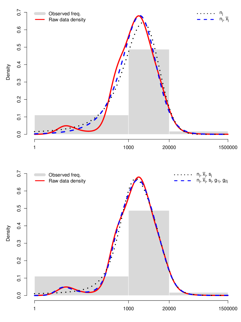
Figure 4: Car insurance data: observed frequencies and density estimates (on the $\log_{10}$-scale) using tabulated sample moments.

				$\text{VaR}_{5\%}$			$\text{VaR}_{1\%}$
Data ${{\cal D}}$	edf	RIMSE	K-L	Est.	95% cred.int.		Est.	95% cred.int.
${{\cal D}}_{0}$	6.2	0.069	0.042	16 250	(14 795, 17 848)		34 764	(29 724, 40 658)
${{\cal D}}_{1}$	6.7	0.030	0.029	15 885	(14 617, 17 263)		41 502	(37 064, 46 472)
${{\cal D}}_{2}$	9.0	0.027	0.019	16 641	(15 355, 17 647)		40 766	(35 261, 47 131)
${{\cal D}}_{4}$	11.7	0.012	0.001	16 106	(14 896, 17 413)		38 988	(33 504, 45 371)

Table 6: Car insurance data: numerical comparison of density and Value-at-Risk estimates obtained using tabulated sample moments of increasing orders.

		Central moments for $\log_{10}$(Claim)
Interval	Freq.		$M_{1}$			$M_{2}$			$M_{3}$			$M_{4}$
$\mathcal{C}_{j}$	$n_{j}$		Obs.	Fitted		Obs.	Fitted		Obs.	Fitted		Obs.	Fitted
(0.00 ; 3.00]	1168		2.462	2.472		0.336	0.336		-0.350	-0.351		0.611	0.619
(3.00 ; 4.30]	2234		3.529	3.532		0.113	0.111		0.014	0.013		0.028	0.026
(4.30 ; 6.18]	116		4.556	4.549		0.075	0.073		0.054	0.051		0.071	0.064

Table 7: Car insurance data: observed and fitted central moments within classes using a model based on ${{\cal D}}_{4}$.

6 Discussion

We have shown how to combine tabulated summary statistics involving moments of order one to four with the observed frequencies to estimate a density from grouped data. The proposed inference strategy, implemented in the R-package degross, relies on an EM algorithm with uncertainty measures computed in a final step from the observed penalized log-likelihood. The penalty not only encourages smoothing of the resulting density estimate, but also ensures agreement up to sampling errors between the underlying theoretical moments and their observed values in each class. Simple parametric alternatives might be considered for the density model in specific settings. The nonparametric estimation studied here could then be used to validate or select such proposals, or to point out their possible shortcomings.

Although the transmission of data using tabulated summary statistics may not be fully compliant with the European General Data Protection Regulation (GDPR, EU 2016/679) guidelines, it enables to mask data details by summarizing them with a couple of technical numbers besides the class frequencies, see e.g. Table 5. This is a convenient method to communicate in a fairly accurate and compact way on the distribution of the underlying raw data with a limited loss of information.

That methodology might be combined with regression models where information on the distribution of the response is provided in such a summarized way conditionnally on a selected and limited number of subject characteristics (such as the age category in the car insurance example). At the individual level, besides covariates values, the reported loss would take the form of a class indicator. The challenge would be to make inference on the regression model components from such imprecise information on the response data. Flexible forms for the error distribution and for the quantification of covariate effect on the response conditional distribution should be compatible with the available information at the aggregate level.

References

- [1] C. Bernard, M. Denuit and S. Vanduffel “Measuring portfolio risk under partial dependence information”, 2014
- [2] P.L. Brocketf, S.H. Cox, B. Golany, F.Y. Phillips and Y. Song “Actuarial usage of grouped data: an approach to incorporating secondary data” In Transactions of Society of Actuaries 47, 1995, pp. 89–113
- [3] A.. Dempster, N.. Laird and D.. Rubin “Maximum likelihood from incomplete data via the EM algorithm” In Journal of the Royal Statistical Society: Series B (Methodological) 39.1, 1977, pp. 1–22 DOI: 10.1111/j.2517-6161.1977.tb01600.x
- [4] Paul H.. Eilers “Ill-posed problems with counts, the composite link model and penalized likelihood” In Statistical Modelling 7.3, 2007, pp. 239–254 DOI: 10.1177/1471082X0700700302
- [5] Paul H.. Eilers and Brian D. Marx “Flexible smoothing with B-splines and penalties” In Statistical Science 11, 1996, pp. 89–102 DOI: 10.1214/ss/1038425655
- [6] Oswaldo Gressani and Philippe Lambert “Laplace approximation for fast Bayesian inference in generalized additive models based on penalized regression splines” In Computational Statistics and Data Analysis, 2021 DOI: 10.1016/j.csda.2020.107088
- [7] L.P. Hansen “Large sample properties of generalized method of moments estimators” In Econometrica 50.4, 1982, pp. 1029–1054 DOI: 10.2307/1912775
- [8] W. Hürlimann “Extremal moment methods and stochastic orders” In Boletin de la Associacion Matematica Venezolana 15, 2008, pp. 153–301
- [9] A. Jullion and P. Lambert “Robust specification of the roughness penalty prior distribution in spatially adaptive Bayesian P-splines models” In Computational Statistics and Data Analysis 51.5, 2007, pp. 2542–2558 DOI: 10.1016/j.csda.2006.09.027
- [10] Philippe Lambert “Fast Bayesian inference using Laplace approximations in nonparametric double additive location-scale models with right- and interval-censored data” In Computational Statistics and Data Analysis, 2021 DOI: 10.1016/j.csda.2021.107250
- [11] Philippe Lambert and Paul H.. Eilers “Bayesian density estimation from grouped continuous data” In Computational Statistics and Data Analysis 53.4, 2009, pp. 1388–1399 DOI: 10.1016/j.csda.2008.11.022
- [12] T. Pentikäinen “Approximative evaluation of the distribution function of aggregate claims” In ASTIN Bulletin 17.1, 1987, pp. 15–39 DOI: 10.2143/AST.17.1.2014982
- [13] Gareth O. Roberts and Jeffrey S. Rosenthal “Optimal scaling of discrete approximations to Langevin diffusions” In Journal of the Royal Statistical Society. Series B: Statistical Methodology 60.1, 1998, pp. 255–268 DOI: 10.1111/1467-9868.00123
- [14] R. Thompson and R.J. Baker “Composite link functions in generalized linear models” In Journal of the Royal Statistical Society. Series C (Applied Statistics) 30.2, 1981, pp. 125–131