Thermal Trigger for Solar Flares III: Effect of the Oblique Layer Fragmentation

1 Introduction

sec1

The magnetic reconnection process is a key mechanism for changing the topology of the magnetic field (Priest and Forbes, 2002). It provides the ability to redistribute independent magnetic fluxes. In a highly conductive plasma like the solar atmosphere, the reconnection process contains an intermediate stage characterized by the formation of a current layer between the interacting magnetic fluxes (Syrovatskii, 1971). The current layer, shielding the approaching flows, does not allow them to reconnect. In the vicinity of the current layer, the free energy of the magnetic field is accumulated, which can be converted into the kinetic energy of plasma particles and electromagnetic radiation as a result of the destruction of the current layer (Shibata and Magara, 2011). We call such an electromagnetic explosion in the solar atmosphere a solar flare (Benz, 2017).

It is assumed that the process of destruction of the current layer can be associated with various plasma instabilities. The well-known tearing instability is an example of such instability of a magnetohydrodynamic (MHD) nature (Furth, Killeen, and Rosenbluth, 1963). Classical tearing instability leads to fragmentation of the current layer along the direction of the current. This fragmentation makes a breach in the shielding created by the current layer from which the fast reconnection process can begin (Somov and Verneta, 1993). However, it is unable to explain the inhomogeneity in the energy release along the direction of the current in the layer observed in solar flares (Reva et al., 2015). There are modifications of the tearing instability that provide oblique fragmentation of the layer, designed to describe such inhomogeneity (Artemyev and Zimovets, 2012).

The thermal instability of the plasma is another type of instability (Field, 1965). It can also explain the inhomogeneity of energy release in solar flares (Somov and Syrovatskii, 1982). We have found an instability of thermal nature in the piecewise homogeneous model of the preflare current layer (Ledentsov, 2021a). Periodic fragmentation of the current layer across the direction of the current is the result of the instability. We assume that such instability can cause the onset of the fast reconnection phase in the current layer. As a result, a quasiperiodic distribution of regions of intense energy release along the current layer is formed. The found spatial period of the instability is in the range of 1–10 Mm for a wide range of assumed parameters of the coronal plasma. This scale is consistent with the observed loop distance in solar flare arcades.

We have also investigated the influence of the guide field on the simulation results (Ledentsov, 2021b). The guide magnetic field is located along the current both outside and inside the current layer. The guide field does not participate in reconnection. However, it affects the pressure balance at the boundary of the current layer and leads to an anisotropy of the transfer coefficients within the layer. We have shown that a weak guide field, suppressing the thermal conductivity inside the current layer, promotes the formation of the instability, but a strong field leads to its stabilization. The spatial scale of the instability remains the same in the expected temperature range of the current layer.

The listed results were obtained under the assumption of an infinite width (along $x$-axis) of the current layer under the condition $\partial/\partial{x}=0$. This made it possible to simplify the derivation of the dispersion relation, while maintaining the physical content of the model. In addition, it also avoids the appearance of the well-known tearing instability, which leads to a similar fragmentation of the current layer along the direction of the current. Physically, the condition $\partial/\partial{x}=0$ means that we consider perturbations propagating only parallel to the direction of the current in the layer. This is the direction we expect to see in the observations, but it is a prescribed condition and not the result of the model itself.

In this article, we want to drop the condition $\partial/\partial{x}=0$ and study how the simulation results change. In Section sec2, we consider an infinitely wide current layer with perturbations propagating in its plane. In Section sec3, we study the dispersion equation properties. In Section sec4, we calculate the spatial scales of the instability for coronal plasma parameters. Conclusions are given in Section sec5.

2 Current Layer Model

sec2

We consider a piecewise homogeneous MHD model of the current layer. The model consists of a current layer located in the $(x,y)$ plane and surrounding plasma (Figure fig1). The current layer has a half-thickness $a$, half-width $b$, temperature $T_{s}$, and density $n_{s}$. We consider the current layer to be thin ($b\gg a$), and henceforth take $b\to\infty$. $T_{0}$ and $n_{0}$ are the temperature and concentration of the surrounding plasma. The magnetic field $B_{0}$ in the unperturbed state is present only outside the current layer. However, it is possible for a perturbation of the magnetic field to penetrate into the layer. The magnetic field is directed against the $x$-axis for positive $y$ and along the $x$-axis for negative $y$. Plasma outside the current layer is considered in the ideal MHD approximation. The effects of electrical and thermal conductivity as well as viscosity are taken into account inside the layer.

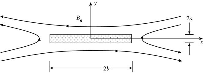
Figure 1.: Location of the current layer in the coordinate system. $a$ is the half-thickness, $b$ is the half-width of the layer.fig1

Plasma behavior is described by the following set of MHD equations (Syrovatskii, 1958; Somov, 2012):

$$\frac{\partial n}{\partial t}+\mathrm{div}\,(n{\mathbfit v})=0\,,$$

$$\mu n\,\frac{\rm{d}{\mathbfit v}}{{\rm d}t}=-{\bf\nabla}(2nk_{{}_{\rm B}}T)-\frac{1}{4\pi}\,({\mathbfit B}\times\mathrm{curl}{\mathbfit B})+\eta\,\Delta{\mathbfit v}+\nu\,{\bf\nabla}\,\mathrm{div}\,{\mathbfit v}\,,$$

$$\frac{2nk_{{}_{\rm B}}}{\gamma-1}\,\frac{{\rm d}T}{{\rm d}t}-2k_{{}_{\rm B}}T\,\frac{{\rm d}n}{{\rm d}t}\\ =\frac{c^{2}}{(4\pi)^{2}\sigma}\,({\mathrm{curl}}{{\mathbfit B}})^{2}+\frac{\partial}{\partial r_{\alpha}}(\sigma_{\alpha\beta}v_{\beta})+{\mathrm{div}}\,(\kappa{\bf\nabla}T)-\lambda\,(n,T)\,,$$

$$\frac{\partial{{\mathbfit B}}}{\partial t}={\mathrm{curl}}\,({{\mathbfit v}}\times{{\mathbfit B}})-\frac{c^{2}}{4\pi}\,{\mathrm{curl}}\left(\frac{1}{\sigma}\,{\mathrm{curl}}{{\mathbfit B}}\right),$$

$${\mathrm{div}}{{\mathbfit B}}=0\,.\ilabel{01}$$ (1)

Here, $\mu=1.44\,m_{H}$, $m_{H}$ is the mass of the hydrogen atom, $k_{{}_{\rm B}}$ is the Boltzmann constant. The heat capacity ratio is assumed $\gamma=5/3$ for simplicity. $T$ is the temperature, $n$ is the plasma density, $v$ is the plasma velocity, and $B$ is the magnetic field. The plasma is assumed to be ideal outside the current layer, while dissipative effects are important inside it: the finite electrical $\sigma$ and thermal $\kappa$ conductivity of the plasma, the viscosity ratios $\eta$, and $\nu$, and the viscous stress tensor $\sigma_{\alpha\beta}$, as well as its radiative cooling $\lambda$. Here $\alpha$ and $\beta$ are tensor indices corresponding to the spatial coordinates $x$, $y$, and $z$. The radiative cooling function $\lambda\,(n,T)=n^{2}L(T)$ contains the total radiative loss function $L(T)$ that is calculated from the CHIANTI 9 atomic database (Dere et al., 2019) for an optically thin medium with coronal abundance of elements (see Figure 1 in Ledentsov, 2021a). The solution of the system of equations for small perturbations will be found separately outside the layer and inside the layer. Then the found solutions will be sewn on the boundary, which is a tangential MHD discontinuity.

2.1 Outside the Current Layer

sec2.1

The plasma is at rest $v_{0}=0$, and the dissipative effects are negligible $\sigma\to\infty$, $\kappa=0$, $\lambda=0$ outside the current layer. The symmetry of the model allows us to consider only the positive $y$. The solution to the problem of small perturbations is assumed to be periodic in the plane of the current layer and decay with distance from the layer:

$$f(y,z,t)=f_{0}+f_{1}(y)\,{\rm exp}\,(-i\omega t+ik_{x}x+ik_{z}z)\,,$$

$$f_{1}(y)=f_{1}\,{\rm exp}\,[-k_{y1}(y-a)]\,,$$

where perturbation amplitudes are

$$f_{1}\equiv\{{v_{x1},v_{y1},v_{z1},n_{1},T_{1},B_{x1},B_{y1},B_{z1}}\}\,,$$

The linearized system of Equations 01 takes the form:

$$i\omega\,n_{1}=ik_{x}\,n_{0}v_{x1}-k_{y1}\,n_{0}v_{y1}+ik_{z}\,n_{0}v_{z1}\,,\ilabel{02}$$ (2)

$$i\omega\,\mu n_{0}v_{x1}=ik_{x}\,2k_{{}_{\rm B}}(n_{0}T_{1}+T_{0}n_{1})\,,\ilabel{03}$$ (3)

$$i\omega\,\mu n_{0}v_{y1}=-k_{y1}\,2k_{{}_{\rm B}}(n_{0}T_{1}+T_{0}n_{1})+k_{y1}\,\frac{B_{0}}{4\pi}\,B_{x1}+ik_{x}\,\frac{B_{0}}{4\pi}\,B_{y1}\,,\ilabel{04}$$ (4)

$$i\omega\,\mu n_{0}v_{z1}=ik_{z}\,2k_{{}_{\rm B}}(n_{0}T_{1}+T_{0}n_{1})-ik_{z}\,\frac{B_{0}}{4\pi}\,B_{x1}+ik_{x}\,\frac{B_{0}}{4\pi}\,B_{z1}\,,\ilabel{05}$$ (5)

$$(\gamma-1)\,T_{0}n_{1}=n_{0}T_{1}\,,\ilabel{06}$$ (6)

$$i\omega\,B_{x1}=k_{y1}\,B_{0}\,v_{y1}-ik_{z}\,B_{0}\,v_{z1}\,,\ilabel{07}$$ (7)

$$i\omega\,B_{y1}=ik_{x}\,B_{0}\,v_{y1}\,,\ilabel{08}$$ (8)

$$i\omega\,B_{z1}=ik_{x}\,B_{0}\,v_{z1}\,.\ilabel{09}$$ (9)

The determinant of a homogeneous system of the linear Equations 02–09 must be equal to zero for a nontrivial solution to exist. Therefore, the dispersion relation

$$k_{y1}^{2}=k_{z}^{2}+\frac{V_{A}^{2}k_{x}^{2}+{\it\Gamma}^{\,2}}{\left(\frac{1}{V_{S}^{2}}+\frac{k_{x}^{2}}{{\it\Gamma}^{\,2}}\right)^{-1}\!\!+V_{A}^{2}}\ilabel{10}$$ (10)

must be fulfilled outside the current layer. Here we have introduced the notation for the sound and Alfvén speeds

$$V_{S}=\sqrt{\frac{2\gamma k_{{}_{\rm B}}T_{0}}{\mu}}\,,\qquad V_{A}=\frac{B_{0}}{\sqrt{4\pi n_{0}\mu}}\,,\qquad$$

as well as the increment of the instability ${\it\Gamma}=-i\omega$.

2.2 Inside the Current Layer

sec2.2

The plasma is also at rest $v_{s}=0$, but the dissipative effects must be considered inside the current layer. The solution is also sought in the form of a sum of a constant term and a perturbation

$$f(y,z,t)=f_{s}+f_{2}(y)\,{\rm exp}\,(-i\omega t+ik_{x}x+ik_{z}z)\,.$$

Following Ledentsov (2021a), we consider the dependence of the perturbation on the coordinate $y$ in the form of a hyperbolic sine for odd perturbations in $y$

$$\left\{\begin{array}[]{c}v_{y2}(y)\\ B_{y2}(y)\end{array}\right\}=\left\{\begin{array}[]{c}v_{y2}\\ B_{y2}\end{array}\right\}{\rm sinh}\,(k_{y2}y)\,$$

and a hyperbolic cosine for even perturbations in $y$

$$\left\{\begin{array}[]{c}v_{x2}(y)\\ v_{z2}(y)\\ n_{2}(y)\\ T_{2}(y)\\ B_{x2}(y)\\ B_{z2}(y)\end{array}\right\}=\left\{\begin{array}[]{c}v_{x2}\\ v_{z2}\\ n_{2}\\ T_{2}\\ B_{x2}\\ B_{z2}\end{array}\right\}{\rm cosh}\,(k_{y2}y)\,.$$

In contrast to Ledentsov (2021a, b), the amplitudes $v_{x2}$ and $B_{x2}$ are chosen to be even to derive a consistent system of linear equations.

Inside the current layer, the linearized system of Equations 01 takes the form:

$$i\omega\,n_{2}=ik_{x}\,n_{s}v_{x2}+k_{y2}\,n_{s}v_{y2}+ik_{z}\,n_{s}v_{z2}\,,\ilabel{11}$$ (11)

$$i\omega\,\mu n_{s}v_{x2}=ik_{x}\,2k_{{}_{\rm B}}(n_{s}T_{2}+T_{s}n_{2})+(k_{z}^{2}+k_{x}^{2}-k_{y2}^{2})\,\eta v_{x2}-i\omega ik_{x}\frac{\nu}{n_{s}}n_{2}\,,\ilabel{12}$$ (12)

$$i\omega\,\mu n_{s}v_{y2}=k_{y2}\,2k_{{}_{\rm B}}(n_{s}T_{2}+T_{s}n_{2})+(k_{z}^{2}+k_{x}^{2}-k_{y2}^{2})\,\eta v_{y2}-i\omega k_{y2}\frac{\nu}{n_{s}}n_{2}\,,\ilabel{13}$$ (13)

$$i\omega\,\mu n_{s}v_{z2}=ik_{z}\,2k_{{}_{\rm B}}(n_{s}T_{2}+T_{s}n_{2})+(k_{z}^{2}+k_{x}^{2}-k_{y2}^{2})\,\eta v_{z2}-i\omega ik_{z}\frac{\nu}{n_{s}}n_{2}\,,\ilabel{14}$$ (14)

$$i\omega\,\frac{2k_{{}_{\rm B}}n_{s}}{\gamma-1}\,T_{2}-i\omega\,2k_{{}_{\rm B}}T_{s}\,n_{2}=(k_{z}^{2}+k_{x}^{2}-k_{y2}^{2})\,\kappa\,T_{2}+\frac{\partial\lambda}{\partial T}\,T_{2}+\frac{\partial\lambda}{\partial n}\,n_{2}\,,\ilabel{15}$$ (15)

$$i\omega\,B_{x2}=(k_{z}^{2}+k_{x}^{2}-k_{y2}^{2})\,\nu_{m}\,B_{x2}\,,\ilabel{16}$$ (16)

$$i\omega\,B_{y2}=(k_{z}^{2}+k_{x}^{2}-k_{y2}^{2})\,\nu_{m}\,B_{y2}\,,\ilabel{17}$$ (17)

$$i\omega\,B_{z2}=(k_{z}^{2}+k_{x}^{2}-k_{y2}^{2})\,\nu_{m}\,B_{z2}\,.\ilabel{18}$$ (18)

The set of Equations 11–18 splits into two sets and, as a consequence, has two dispersion relations at once. Equations 16–18 under the assumption of a nonzero magnetic perturbation give the dispersion relation

$$k_{y2}^{2}=k_{z}^{2}+k_{x}^{2}+\frac{{\it\Gamma}}{\nu_{m}}\,,\ilabel{20}$$ (19)

where

$$\nu_{m}=\frac{c^{2}}{4\pi\sigma}\,$$

is the magnetic viscosity.

Using Equation 20 we can eliminate the wave numbers $k_{x}$, $k_{y2}$, and $k_{z}$ from Equations 11–15 and determine the increment of the instability

$${\it\Gamma}=\frac{2}{5}\,\frac{\beta-\alpha}{\tau_{\lambda}}\,.\ilabel{21}$$ (20)

For details, see the derivation of Equation 33 in Ledentsov (2021a). The notations for the logarithmic derivatives of the cooling function

$$\alpha=\frac{\partial{\rm\,ln}\,\lambda}{\partial{\rm\,ln}\,T}\,,\qquad\beta=\frac{\partial{\rm\,ln}\,\lambda}{\partial{\rm\,ln}\,n}\,$$

and characteristic time of the radiative cooling

$$\tau_{\lambda}=\frac{2k_{{}_{\rm B}}T_{s}n_{s}}{\lambda}\,$$

are introduced in Equation 21.

2.3 Boundary of the Current Layer

sec2.3

The tangential discontinuity is located at the boundary of the current layer. Zero plasma velocity ($v_{0}=0,v_{s}=0$) and the absence of a component of the magnetic field normal to the discontinuity surface indicate this (Ledentsov and Somov, 2015). The boundary condition for the tangential discontinuity is that the total gas and magnetic pressures on both sides of the discontinuity are equal (Syrovatskii, 1956)

$$2k_{{}_{\rm B}}n_{0}T_{0}+\frac{B_{0}^{2}}{8\pi}=2k_{{}_{\rm B}}n_{s}T_{s}\,.\ilabel{22}$$ (21)

In addition, velocity perturbations $v_{x},v_{y},v_{z}$ will lead to a wave-like curvature of the discontinuity surface (Ledentsov, 2021a). The linearized boundary conditions are written as follows:

$$n_{0}T_{1}+T_{0}n_{1}-\frac{B_{0}B_{x1}}{8\pi k_{{}_{\rm B}}}=(n_{s}T_{2}+T_{s}n_{2})\,{\rm cosh}\,(k_{y2}a)\,,\ilabel{23}$$ (22)

$$v_{y1}=\pm\,v_{y2}\,{\rm sinh}\,(k_{y2}a)\,.\ilabel{24}$$ (23)

We express Equation 23 in terms of perturbation $v_{y1}$ and $v_{y2}$ using Equations 04, 08, and 11–14. Then we divide Equation 24 by Equation 23

$$\pm\,\frac{\tau_{\nu}}{\tau_{\sigma}}\frac{n_{s}}{n_{0}}\,k_{y1}=\left(1+V_{A}^{2}\frac{k_{x}^{2}}{{\it\Gamma}^{\,2}}\right)k_{y2}\,{\rm tanh}\,(k_{y2}a)\,,\ilabel{25}$$ (24)

where

$$\frac{\tau_{\nu}}{\tau_{\sigma}}=1-\frac{\eta+\nu}{\mu n_{s}\,\nu_{m}}\,.$$

For details about characteristic times $\tau_{\nu}$ and $\tau_{\sigma}$, see Equation 9 in Ledentsov (2021a). Wave numbers $k_{y1}$ and $k_{y2}$ can be eliminated from Equation 25 by using Equations 10 and 20, respectively

$$\left(\frac{\tau_{\nu}}{\tau_{\sigma}}\frac{n_{s}}{n_{0}}\right)^{2}\left(k_{z}^{2}+\frac{V_{A}^{2}k_{x}^{2}+{\it\Gamma}^{\,2}}{\left(\frac{1}{V_{S}^{2}}+\frac{k_{x}^{2}}{{\it\Gamma}^{\,2}}\right)^{-1}\!\!+V_{A}^{2}}\right)$$

$$=\left(1+V_{A}^{2}\frac{k_{x}^{2}}{{\it\Gamma}^{\,2}}\right)^{2}\left(k_{z}^{2}+k_{x}^{2}+\frac{{\it\Gamma}}{\nu_{m}}\right)\,{\rm tanh}^{2}\,\left[\left(k_{z}^{2}+k_{x}^{2}+\frac{{\it\Gamma}}{\nu_{m}}\right)^{\!1/2}\!\!a\right]\,.$$ (25)

The dispersion Equation 26 is equivalent to the dispersion Equation 32 from Ledentsov (2021a) for $k_{x}=0$.

Equation 26 has thin and thick approximations depending on the value under the hyperbolic tangent.

$$k_{z{\rm thin}}^{2}\simeq\left(\frac{(1+V_{A}^{2}\frac{k_{x}^{2}}{{\it\Gamma}^{\,2}})(k_{z}^{2}+k_{x}^{2}+\frac{{\it\Gamma}}{\nu_{m}})a}{\frac{\tau_{\nu}}{\tau_{\sigma}}\frac{n_{s}}{n_{0}}}\right)^{\!2}\!\!-\frac{V_{A}^{2}k_{x}^{2}+{\it\Gamma}^{\,2}}{\left(\frac{1}{V_{S}^{2}}+\frac{k_{x}^{2}}{{\it\Gamma}^{\,2}}\right)^{-1}\!\!+V_{A}^{2}}\,\ilabel{27}$$ (26)

for ${\rm tanh}\,x\simeq x$ and

$$k_{z{\rm thick}}^{2}\simeq\frac{(1+V_{A}^{2}\frac{k_{x}^{2}}{{\it\Gamma}^{\,2}})^{2}(k_{z}^{2}+k_{x}^{2}+\frac{{\it\Gamma}}{\nu_{m}})}{\left(\frac{\tau_{\nu}}{\tau_{\sigma}}\frac{n_{s}}{n_{0}}\right)^{2}}-\frac{V_{A}^{2}k_{x}^{2}+{\it\Gamma}^{\,2}}{\left(\frac{1}{V_{S}^{2}}+\frac{k_{x}^{2}}{{\it\Gamma}^{\,2}}\right)^{-1}\!\!+V_{A}^{2}}\,\ilabel{28}$$ (27)

for ${\rm tanh}\,x\simeq 1$. If we use the assumption ${{\it\Gamma}}/{\nu_{m}}\gg k^{2}$ which was fulfilled for coronal plasma with great accuracy in Ledentsov (2021a) and neglect viscosity and the second terms in the Equations 27 and 28, we find

$$k_{z{\rm thin}}\simeq\left(1-\frac{V_{A}^{2}}{V_{x}^{2}}\right)\frac{n_{0}}{n_{s}}\,\frac{{\it\Gamma}}{V_{D}}\,,\ilabel{29}$$ (28)

$$k_{z{\rm thick}}\simeq\left(1-\frac{V_{A}^{2}}{V_{x}^{2}}\right)\frac{n_{0}}{n_{s}}\sqrt{\frac{{\it\Gamma}}{\nu_{m}}}\,,\ilabel{30}$$ (29)

where $V_{D}=\nu_{m}/a$ is the drift velocity and $V_{x}^{2}=-({\it\Gamma}/k_{x})^{2}$ is the square of the $x$-component of the phase velocity of the perturbation. It will be shown in Section sec4 that Equations 29 and 30 are good simple approximations of the exact dispersion relation for the coronal plasma.

3 Dispersion Equation Properties

sec3

The dispersion Equation 26 connects $k_{x}$, $k_{z}$, and ${\it\Gamma}$. The instability increment ${\it\Gamma}$ is independently determined by Equation 21. However, $k_{z}$ can be determined not for every $k_{x}$ from Equation 26 for a given ${\it\Gamma}$. We will demonstrate this as follows. Let us introduce the function

$$g({\it\Gamma},k_{x},k_{z})=\left(\frac{\tau_{\nu}}{\tau_{\sigma}}\frac{n_{s}}{n_{0}}\right)^{2}\left(k_{z}^{2}+\frac{V_{A}^{2}k_{x}^{2}+{\it\Gamma}^{\,2}}{\left(\frac{1}{V_{S}^{2}}+\frac{k_{x}^{2}}{{\it\Gamma}^{\,2}}\right)^{-1}\!\!+V_{A}^{2}}\right)$$

$$-\left(1+V_{A}^{2}\frac{k_{x}^{2}}{{\it\Gamma}^{\,2}}\right)^{2}\left(k_{z}^{2}+k_{x}^{2}+\frac{{\it\Gamma}}{\nu_{m}}\right)\,{\rm tanh}^{2}\,\left[\left(k_{z}^{2}+k_{x}^{2}+\frac{{\it\Gamma}}{\nu_{m}}\right)^{\!1/2}\!\!a\right]\,.$$

The dispersion Equation 26 defines the zeros of this function. If the function $g$ has no zeros for some given ${\it\Gamma}$ and $k_{x}$, then the dispersion Equation 26 has no corresponding solutions. We use characteristic conditions of the coronal plasma of an active region $n_{0}=10^{10}$ cm^-3, $n_{s}=10^{11}$ cm^-3, $T_{0}=10^{6}$ K, $T_{s}=10^{7}$ K, $a=10^{5}$ cm, $\sigma=10^{11}$ s^-1 (Somov, 2013). The magnetic field $B_{0}$ is determined by Equation 22 and is usually about 100 G, ${\it\Gamma}$ is determined by Equation 21.

Figure fig2 shows the dependence of the function $g$ on the wave number $k_{z}$ (Figure fig2a) and on the spatial period $l_{z}=2\pi/k_{z}$ (Figure fig2b) for three values of the wave number $k_{x}$: $10^{-9.15}$ cm^-2 (dotted lines), $10^{-9.20}$ cm^-2 (dashed lines), $10^{-9.25}$ cm^-2 (solid lines). There is a value $k_{x{\rm max}}$ at which the function $g$ touches the $k_{z}$-axis . The function $g$ has zeros for $k_{x}\leq k_{x{\rm max}}$ and does not have zeros for $k_{x}>k_{x{\rm max}}$. Thus, the dispersion Equation 26 has solutions only for $k_{x}\leq k_{x{\rm max}}$ for each given ${\it\Gamma}$. The function $g$ has two zeros for $k_{x}<k_{x{\rm max}}$. With decreasing $k_{x}$, the lower zero in Figure fig2a tends to the value corresponding to the dispersion Equation 32 from Ledentsov (2021a), while the larger zero quickly tends to infinity and disappears for

$$\frac{\tau_{\nu}}{\tau_{\sigma}}\frac{n_{s}}{n_{0}}>1+V_{A}^{2}\frac{k_{x}^{2}}{{\it\Gamma}^{\,2}}\,.$$

For this reason, in what follows we will consider solutions of dispersion equations corresponding only to the lower zero of the function $g$.

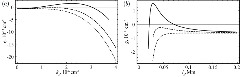
Figure 2.: $g$ as a function (a) of the wave number $k_{z}$ and (b) of the spatial period $l_{z}$ for three values of the wave number $k_{x}$: $10^{-9.15}$ cm^-2 (dotted lines), $10^{-9.20}$ cm^-2 (dashed lines), $10^{-9.25}$ cm^-2 (solid lines). fig2

Let us find the maximum wave numbers $k_{x{\rm max}}$ and $k_{z{\rm max}}$. They correspond to the contact of the function $g(k_{z})$ and $k_{z}$-axis. The maximum point of the function $g(k_{z})$ is determined by the equation

$$\left(\frac{\frac{\tau_{\nu}}{\tau_{\sigma}}\frac{n_{s}}{n_{0}}}{1+V_{A}^{2}\frac{k_{x}^{2}}{{\it\Gamma}^{\,2}}}\right)^{2} = {\rm tanh}^{2}\,\left[\left(k_{z}^{2}+k_{x}^{2}+\frac{{\it\Gamma}}{\nu_{m}}\right)^{\!1/2}\!\!a\right]$$ (30)

$$+ a\,(k_{z}^{2}+k_{x}^{2}+\frac{{\it\Gamma}}{\nu_{m}})^{\!1/2}\,\frac{{\rm tanh}\,\left[\left(k_{z}^{2}+k_{x}^{2}+\frac{{\it\Gamma}}{\nu_{m}}\right)^{\!1/2}\!\!a\right]}{{\rm cosh}^{2}\,\left[\left(k_{z}^{2}+k_{x}^{2}+\frac{{\it\Gamma}}{\nu_{m}}\right)^{\!1/2}\!\!a\right]}\,.$$

Figure fig2a shows that $k_{z{\rm max}}\gg k_{x{\rm max}}$. Then in the thin approximation, we have from Equations 27 and 31

$$\left(\frac{\frac{\tau_{\nu}}{\tau_{\sigma}}\frac{n_{s}}{n_{0}}}{1+V_{A}^{2}\frac{k_{x{\rm thin}}^{2}}{{\it\Gamma}^{\,2}}}\right)^{2}\simeq\frac{a^{2}}{k_{z{\rm thin}}^{2}}\left(k_{z{\rm thin}}^{2}+\frac{{\it\Gamma}}{\nu_{m}}\right)^{\!2}\,,$$

$$\left(\frac{\frac{\tau_{\nu}}{\tau_{\sigma}}\frac{n_{s}}{n_{0}}}{1+V_{A}^{2}\frac{k_{x{\rm thin}}^{2}}{{\it\Gamma}^{\,2}}}\right)^{2}\simeq 2a^{2}\left(k_{z{\rm thin}}^{2}+\frac{{\it\Gamma}}{\nu_{m}}\right)\,,$$

respectively. From here

$$k_{z{\rm thinmax}}^{2}\simeq\frac{{\it\Gamma}}{\nu_{m}}\,,\qquad k_{x{\rm thinmax}}^{2}\simeq\left(\frac{\tau_{\nu}}{\tau_{\sigma}}\,\frac{n_{s}}{n_{0}}\,\frac{1}{2a}\sqrt{\frac{\nu_{m}}{{\it\Gamma}}}-1\right)\left(\frac{{\it\Gamma}}{V_{A}}\right)^{\!2}\,.\ilabel{32}$$ (31)

In the thick approximation, we have from Equations 28 and 31

$$\left(\frac{\frac{\tau_{\nu}}{\tau_{\sigma}}\frac{n_{s}}{n_{0}}}{1+V_{A}^{2}\frac{k_{x{\rm thick}}^{2}}{{\it\Gamma}^{\,2}}}\right)^{2}\simeq\frac{1}{k_{z{\rm thick}}^{2}}\left(k_{z{\rm thick}}^{2}+\frac{{\it\Gamma}}{\nu_{m}}\right)\,,$$

$$\left(\frac{\frac{\tau_{\nu}}{\tau_{\sigma}}\frac{n_{s}}{n_{0}}}{1+V_{A}^{2}\frac{k_{x{\rm thick}}^{2}}{{\it\Gamma}^{\,2}}}\right)^{2}\simeq 1\,,$$

respectively, and

$$k_{z{\rm thickmax}}^{2}\gg\frac{{\it\Gamma}}{\nu_{m}}\,,\qquad k_{x{\rm thickmax}}^{2}\simeq\left(\frac{\tau_{\nu}}{\tau_{\sigma}}\,\frac{n_{s}}{n_{0}}-1\right)\left(\frac{{\it\Gamma}}{V_{A}}\right)^{\!2}\,.\ilabel{33}$$ (32)

We use Equations 32 and 33 in Section sec4 to compare the spatial scales of instability $l_{x}=2\pi/k_{x}$ and $l_{z}=2\pi/k_{z}$.

4 Spatial Scales of the Instability

sec4

The spatial scales of the instability $l_{x}=2\pi/k_{x}$ and $l_{z}=2\pi/k_{z}$ are determined by the dispersion Equation 26 and its simple approximations (Equations 29 and 30). Figures fig3 and fig4 show the relationship between the spatial scales of the instability calculated from Equation 26 (squares). Thin (Equation 29) and thick (Equation 30) approximations are also shown in Figures fig3 and fig4 with solid and dashed lines, respectively. The temperature of the surrounding plasma $T_{0}=10^{6}$ K and the temperature of the current layer $T_{s}=10^{7}$ K were used for calculations. Figures fig3 and fig4 show calculation results for concentrations of the surrounding plasma $n_{0}=10^{10}$ cm^-3 and $n_{0}=10^{9}$ cm^-3, respectively. The density contrast is the same $n_{s}/n_{0}=10$ for all calculations. The parameters of the current layer $a$ and $\sigma$ are indicated in the figure caption. The increment of the instability ${\it\Gamma}$ and the magnetic field strength $B_{0}$ were calculated from Equations 21 and 22, respectively. The minimum values for the thin and thick approximations are taken from Equations 32 and 33, respectively.

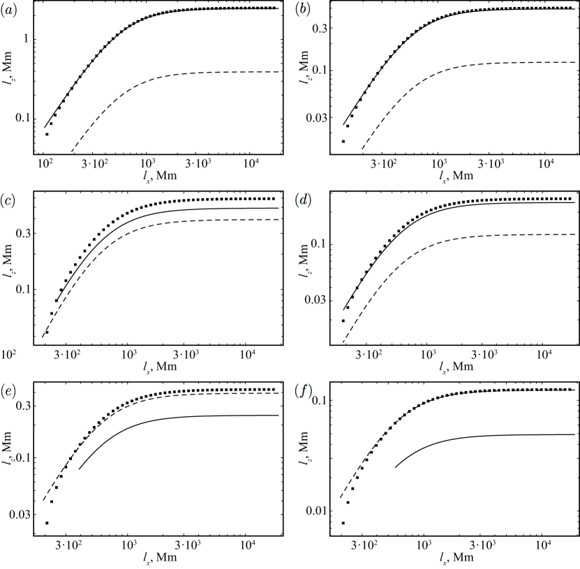
Figure 3.: The relationship between the spatial scales of the instability $l_{x}$ and $l_{z}$ calculated from Equation 26 with $n_{0}=10^{10}$ and $n_{s}=10^{11}$ (squares). Thin (Equations 29) and thick (Equations 30) approximations are shown with solid and dashed lines, respectively. Parameters of the current layer: (a) $a=10^{5}{\rm\,cm}$, $\sigma=10^{11}{\rm\,s}^{-1}$, (b) $a=5\times 10^{4}{\rm\,cm}$, $\sigma=10^{12}{\rm\,s}^{-1}$, (c) $a=5\times 10^{5}{\rm\,cm}$, $\sigma=10^{11}{\rm\,s}^{-1}$, (d) $a=10^{5}{\rm\,cm}$, $\sigma=10^{12}{\rm\,s}^{-1}$, (e) $a=10^{6}{\rm\,cm}$, $\sigma=10^{11}{\rm\,s}^{-1}$, (f) $a=5\times 10^{5}{\rm\,cm}$, $\sigma=10^{12}{\rm\,s}^{-1}$. fig3

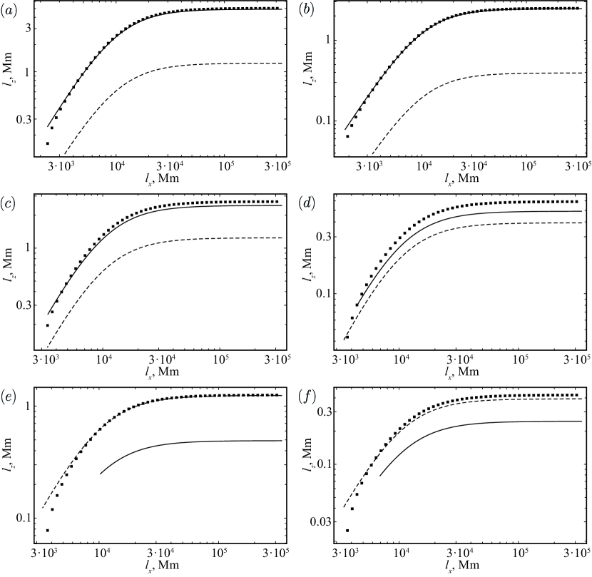
Figure 4.: The relationship between the spatial scales of the instability $l_{x}$ and $l_{z}$ calculated from Equation 26 with $n_{0}=10^{9}$ and $n_{s}=10^{10}$ (squares). Thin (Equations 29) and thick (Equations 30) approximations are shown with solid and dashed lines, respectively. Parameters of the current layer: (a) $a=5\times 10^{5}{\rm\,cm}$, $\sigma=10^{11}{\rm\,s}^{-1}$, (b) $a=10^{5}{\rm\,cm}$, $\sigma=10^{12}{\rm\,s}^{-1}$, (c) $a=10^{6}{\rm\,cm}$, $\sigma=10^{11}{\rm\,s}^{-1}$, (d) $a=5\times 10^{5}{\rm\,cm}$, $\sigma=10^{12}{\rm\,s}^{-1}$, (e) $a=5\times 10^{6}{\rm\,cm}$, $\sigma=10^{11}{\rm\,s}^{-1}$, (f) $a=10^{6}{\rm\,cm}$, $\sigma=10^{12}{\rm\,s}^{-1}$. fig4

Figures fig3 and fig4 have several features.

1) All squares in Figures fig3 and fig4 go out to the value of the spatial scale $l_{z}$ calculated in the model with $\partial/\partial{x}=0$ (Ledentsov, 2021a) when the spatial scale $l_{x}$ increases. The spatial scale $l_{z}$ decreases at small $l_{x}$. However, the reduction in the scale $l_{z}$ is approximately an order of magnitude for the minimal scale $l_{x}$. This indicates a weak influence of the oblique fragmentation of the current layer on the model results.

2) Squares in Figures fig3 and fig4 are in good agreement with the thin or thick approximation, depending on the selected half-thickness $a$ of the current layer. The largest discrepancies occur at the minimum values $l_{z}$. This is due to the fact that in these values the assumption ${{\it\Gamma}}/{\nu_{m}}\gg k^{2}$ used to derive Equations 29 and 30 is not correct (see Equations 32 and 33).

3) Figures fig3 and fig4 allow us to determine the maximum angle of propagation of the perturbation in relation to the direction of the current in the layer. It is equal to the angle of inclination of the tangent to the graph of the function $l_{z}(l_{x})$ passing through the origin. For the dependencies shown in Figures fig3 and fig4, it does not exceed $0.2^{\circ}$ and decreases with increasing layer thickness and plasma conductivity and decreasing concentration of the surrounding plasma. This value can increase for other realistic parameters of the coronal plasma due to an increase in the instability scale for extremely thin current layers ($a\approx 10^{4}$ cm), but not more than 10 times (up to $2^{\circ}$). Hence, it follows that fragmentation transverse to the current is a natural property of the thermal instability of the current layer model under consideration.

5 Conclusion

sec5

Earlier, we studied the stability of piecewise homogeneous current layer models (Ledentsov, 2021a, b) with respect to small perturbations and discovered an instability of thermal nature. The instability resulted in fragmentation of the current layer across the direction of the current. However, the direction of fragmentation was determined by the search for a wave solution propagating along the current. In this article, we remove the restriction on the direction of the wave solution. We estimate the possibility of an oblique fragmentation formation as a result of the thermal instability of the current layer.

We found the dispersion Equation 26 for the thermal instability of the infinitely wide current layer and its simple approximations (Equations 29 and 30). It is shown that the dispersion Equation 26 has no solutions for sufficiently small spatial periods of the instability. Equations 32 and 33 estimate the maximum wave numbers of the instability.

The influence of the oblique propagation of the perturbation on the model results is generally insignificant, but extreme changes can reach an order of magnitude (Figures fig3 and fig4). Thus, oblique fragmentation can lead to a decrease in the estimate of the spatial period of localization of elementary energy release in solar flares to 0.1–1 Mm instead of 1–10 Mm obtained earlier.

We have established that fragmentation transverse to the current is a natural feature of the model. The maximum deviation of the wave vector of the perturbation from the direction of the current does not exceed $0.2^{\circ}$ for the considered examples. This value can increase for extremely thin current layers, but not more than $2^{\circ}$ for the realistic parameters of the coronal plasma.

Disclosure of Potential Conflicts of Interest The author declares that there are no conflicts of interest.

References

- Artemyev and Zimovets (2012) Artemyev, A., Zimovets, I.: 2012, Stability of Current Sheets in the Solar Corona. Sol. Phys. 277, 283. DOI. ADS.
- Benz (2017) Benz, A.O.: 2017, Flare Observations. Living Rev. Sol. Phys. 14, 2. DOI. ADS.
- Dere et al. (2019) Dere, K.P., Del Zanna, G., Young, P.R., Landi, E., Sutherland, R.S.: 2019, CHIANTI—An Atomic Database for Emission Lines. XV. Version 9, Improvements for the X-Ray Satellite Lines. ApJS 241, 22. DOI. ADS.
- Field (1965) Field, G.B.: 1965, Thermal Instability. ApJ 142, 531. DOI. ADS.
- Furth, Killeen, and Rosenbluth (1963) Furth, H.P., Killeen, J., Rosenbluth, M.N.: 1963, Finite-Resistivity Instabilities of a Sheet Pinch. Phys. Fluids 6, 459. DOI. ADS.
- Ledentsov (2021a) Ledentsov, L.: 2021a, Thermal Trigger for Solar Flares I: Fragmentation of the Preflare Current Layer. Sol. Phys. 296, 74. DOI. ADS.
- Ledentsov (2021b) Ledentsov, L.: 2021b, Thermal Trigger for Solar Flares II: Effect of the Guide Magnetic Field. Sol. Phys. 296, 93. DOI. ADS.
- Ledentsov and Somov (2015) Ledentsov, L.S., Somov, B.V.: 2015, Discontinuous plasma flows in magnetohydrodynamics and in the physics of magnetic reconnection. Phys. Uspekhi 58, 107. DOI. ADS.
- Priest and Forbes (2002) Priest, E.R., Forbes, T.G.: 2002, The magnetic nature of solar flares. A&A Rev. 10, 313. DOI. ADS.
- Reva et al. (2015) Reva, A., Shestov, S., Zimovets, I., Bogachev, S., Kuzin, S.: 2015, Wave-like Formation of Hot Loop Arcades. Sol. Phys. 290, 2909. DOI. ADS.
- Shibata and Magara (2011) Shibata, K., Magara, T.: 2011, Solar Flares: Magnetohydrodynamic Processes. Living Rev. Sol. Phys. 8, 6. DOI. ADS.
- Somov (2012) Somov, B.V.: 2012, Plasma Astrophysics. Part I: Fundamentals and Practice, 2nd edn. 391, Astrophys. Space Sci. Library, ASSL. DOI. ADS.
- Somov (2013) Somov, B.V.: 2013, Plasma Astrophysics. Part II: Reconnection and Flares, 2nd edn. 392, Astrophys. Space Sci. Library, ASSL. DOI. ADS.
- Somov and Syrovatskii (1982) Somov, B.V., Syrovatskii, S.I.: 1982, Thermal Trigger for Solar Flares and Coronal Loops Formation. Sol. Phys. 75, 237. DOI. ADS.
- Somov and Verneta (1993) Somov, B.V., Verneta, A.I.: 1993, Tearing Instability of Reconnecting current Sheets in Space Plasmas. Space Sci. Rev. 65, 253. DOI. ADS.
- Syrovatskii (1956) Syrovatskii, S.I.: 1956, Some properties of discontinuity surfaces in magnetohydrodynamics. Tr. Fiz. Inst. im. P.N. Lebedeva, Akad. Nauk SSSR [in Russian] 8, 13.
- Syrovatskii (1958) Syrovatskii, S.I.: 1958, Magnetohydrodynamik. Fortschritte der Physik 6, 437. DOI. ADS.
- Syrovatskii (1971) Syrovatskii, S.I.: 1971, Formation of Current Sheets in a Plasma with a Frozen-in Strong Magnetic Field. Soviet Journal of Experimental and Theoretical Physics 33, 933. ADS.