Bootstrapping Generalization of
Process Models Discovered From Event Data

Abstract

Process mining extracts value from the traces recorded in the event logs of IT-systems, with process discovery the task of inferring a process model for a log emitted by some unknown system. Generalization is one of the quality criteria applied to process models to quantify how well the model describes future executions of the system. Generalization is also perhaps the least understood of those criteria, with that lack primarily a consequence of it measuring properties over the entire future behavior of the system when the only available sample of behavior is that provided by the log. In this paper, we apply a bootstrap approach from computational statistics, allowing us to define an estimator of the model’s generalization based on the log it was discovered from. We show that standard process mining assumptions lead to a consistent estimator that makes fewer errors as the quality of the log increases. Experiments confirm the ability of the approach to support industry-scale data-driven systems engineering.

Keywords: Process mining, generalization, bootstrapping, consistent estimator.

1 Introduction

Given an event log that records traces of some real-world system, the challenge of process discovery is to develop a plausible model of that system, so that the behavior of the system can be analyzed independently of the specific transactions included in that particular log. Many different models might be constructed from the same log. Thus, it is important to have tools that allow the quality of a given model to be quantified relative to the initial log. For example, precision is the fraction of the traces permitted by the model that appear in the log, and recall is the fraction of the log’s traces that are valid according to the model. Composite measures have also been defined [1, 8].

A log is only a sample of observations in regard to the underlying system, and not a specification of its actions. It is thus interesting to consider generalization – the extent to which the inferred model accounts for future observations of the system. Generalization poses substantial challenges, since, by its very definition, it asks about behaviors that have not been observed from a system that is not known. High generalization (and high recall) can be obtained by allowing all possible traces. But overly-permissive models of necessity compromise precision. What is desired is a model that attains high precision and recall with respect to the supplied log, and continues to score well on the universe of possible logs that might arise via continued observation. Note that process mining generalization as studied in this work differs from generalization as it applies to process model abstraction [21]. Process model abstraction considers techniques for combining several processes, activities, and events into corresponding generalized concepts, for example, identifying a semantically coherent sub-process in a process model.

In particular, we study the problem of measuring the generalization of a discovered process model, making use of the bootstrapping technique from computational statistics [12]. In the simplest form, the idea is to construct multiple sampled replicates of the initial log, each representing a log that might have emerged from the system. Any aggregate properties established by considering the set of replicates can then be assumed to be valid for the universe of possible traces. That is, by constructing a process model from one replicate, and then testing on another, generalization can be explored. In terms of high-level contributions, our work here:

• Presents, for the first time, an estimator of the generalization of a process model discovered from an event log, grounded in the bootstrap method;

• Shows that the estimator is consistent for the class of systems captured as directly-follows graphs (DFGs), making fewer errors on larger log replicates; and

• Confirms via experiments the feasibility of the new approach in industrial settings.

The next section introduces several key ideas, and a running example. Section 3 presents our new approach, and demonstrates its consistency. Section 4 provides an evaluation that confirms the consistency and feasibility of our approach. Related work is discussed in Section 5. Finally, Section 6 concludes our presentation.

2 Background

2.1 Systems, Models, Logs, and Their Languages

For the purpose of formalizing the problem of measuring generalization of a process model discovered from an event log of a system, consistent with the standard formalization in process mining [7, 1], we interpret the system, model, and log as collections of traces, where a trace is a sequence of actions that attains, or might attain, some goal.

Let ${\Lambda}$ be a set of possible actions; ${\Lambda}=\left\{\texttt{a}\mathchar 44\relax\penalty 0\texttt{b}\mathchar 44\relax\penalty 0\texttt{c}\mathchar 44\relax\penalty 0\texttt{d}\mathchar 44\relax\penalty 0\texttt{e}\mathchar 44\relax\penalty 0\texttt{f}\right\}$ will be used throughout this section. Define ${{\Lambda}^{*}}$ to be the set of all possible traces over ${\Lambda}$, each a finite sequence of actions. Both abbcf and addef are traces over ${\Lambda}$, as is the empty trace, denoted by ${\epsilon}$.

Systems. A system $S$ is a group of active elements, such as software components and agents, that perform actions and thereby consume, produce, or manipulate objects and information. A system can be an information system or a business process with its organization context, business rules, and resources [7]. Any sequence of actions that leads to the system’s goal constitutes a trace. In general, a system might generate an infinite collection of traces, possibly containing infinitely many distinct traces, and hence also possibly containing traces of arbitrary length.

Models. A process model, or just a model, $M$ is a finite description of a set of traces. Figure 1a describes a process model, represented as a directly-follows graph (DFG), with start node $i$, final node $o$, and all walks from $i$ to $o$ as valid traces. That example model, for instance, describes traces abcf and adeef; but does not describe abbcf.

(a)

(b)

Figure 1: (a) An example process model, and (b) an example system.

Logs. An event log, or just a log, $L$ is a finite multiset of traces.

Languages. A language is a subset of the traces in ${\Lambda^{*}}$. The language of system $S$ is the set of all traces $S$ can generate; the language of model $M$ is the set of traces described by $M$; and the language of log $L$ is its support set, ${\mathit{Supp}\left({L}\right)}$. Further, define $\mathcal{L}\subset{\mathcal{P}\!\left({{\Lambda^{*}}}\right)}$, $\mathcal{M}\subseteq{\mathcal{P}\!\left({{\Lambda^{*}}}\right)}$, and $\mathcal{S}\subseteq{\mathcal{P}\!\left({{\Lambda^{*}}}\right)}$ to be sets containing all possible languages of logs, models, and systems, respectively, with $\mathcal{L}$ restricted to finite languages. When the context is clear, we will interpret logs, models, and systems as their languages – if we say that model $M$ was discovered from log $L$ out of system $S$, we may be referring to the concrete system, model, and log, or may be referring to the languages they describe.

2.2 Process Discovery

Given a log, the process discovery problem consists of constructing a model that represents the behavior recorded in the log [1]. For example, using superscripts to indicate multiplicity, let $L=[{{\texttt{abbbcf}}^{5}}\mathchar 44\relax\penalty 0{{\texttt{abcf}}^{20}}\mathchar 44\relax\penalty 0{{\texttt{addef}}}\mathchar 44\relax\penalty 0{{\texttt{adeef}}^{10}}\mathchar 44\relax\penalty 0{{\texttt{adefabcfadef}}^{10}}\mathchar 44\relax\penalty 0{{\texttt{adef}}^{20}}]$ be an event log that contains six distinct traces and 66 traces in total. Many comprehensive process discovery techniques have been devised over the last two decades [1]. However, model $M$, shown in Fig. 1a, can be constructed from $L$ via a simple four-stage discovery algorithm: (1) filter out infrequent traces by, for example, removing the least frequent third of the distinct traces; (2) for every action in each remaining trace, construct a node representing that action; (3) for every pair of adjacent actions $x$ and $y$, introduce a directed edge from the node for $x$ to the node for $y$; and (4) introduce start node $i$ and end node $o$, together with edges from $i$ to every initial action in a frequent trace, and from every last action in a frequent trace to the sink node $o$.

Despite the simplicity of that supposed construction process, $M$ fits $60$ of the traces in $L$, failing on only six. On the other hand, the cycles in $M$ mean that it represents infinitely many traces not present in $L$. To quantify the extent of the mismatch between $L$ and $M$, the measures recall and precision can be used [7, 8, 22]. Given a suite of possible models, precision and recall allow alternative models to be numerically compared.

2.3 Generalization

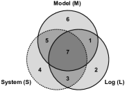
Figure 2: Venn diagram showing languages of model $M$, log $L$, and system $S$, adapted from Buijs et al. [7]; the language of the system is unknown (the dotted border).

An event log of a system contains traces that the system generated over some finite period and were recorded using some logging mechanism. That is, a log is a sample of all possible traces the system could have generated [26]. Hence, an alternative (and arguably more useful) definition of the process discovery problem is that a model be constructed to represent all of the traces the system could have generated, derived from the finite sample provided in the log. Such a model, if constructed, would explain the system, and not just the traces that happened to be recorded in that particular log. For example, the DFG $S$ in Fig. 1b could be a complete representation of the system that generated the 66 traces contained in $L$, allowing, for example, the five occurrences of abbbcf to now be understood.

If the alternative definition of the process discovery problem is accepted, then the candidate model $M$ in Fig. 1a must be somehow benchmarked against the system $S$ of Fig. 1b, rather than against $L$. Unfortunately, the actual behavior of the system is often unknown; indeed, that absence is, of course, a primary motivation for process discovery. That is, the log may be the only available information in respect of the system whose behavior it is a sample of. Given this context, Figure 2 shows the relationship between the languages of log, model, and system. The numbered regions then have the following interpretations (again, making use of example log $L$, model $M$, and system $S$): (1) Traces that $S$ does not generate, yet appear in $L$ (perhaps by error) and are included in $M$; e.g., adeef. (2) Traces that $S$ does not generate, yet appear in $L$ without triggering inclusion in $M$; e.g., addef. (3) Traces permitted by $S$, and recorded in $L$, but not included in $M$; e.g., abbbcf. (4) Traces permitted by $S$, but neither observed in $L$ nor permitted by $M$; e.g., abbcf. (5) Traces permitted by both $S$ and $M$, but not appearing in $L$; e.g., adefadef. (6) Traces neither permitted by $S$ nor observed in $L$, but nevertheless allowed by $M$; e.g., adeeef. (7) Traces permitted by $S$, observed in $L$, and included in $M$; e.g., adefabcfadef. Note that categories (4), (5), and (6) might be infinite, but that (1), (2), (3), and (7) must be finite, as $L$ itself is finite.

To assess a process model against a system, a generalization measure is employed [1]. The objective of a generalization measure is described by van der Aalst [2] as:

a generalization measure […] aims to quantify the likelihood that new unseen [traces generated by the system] will fit the model.

On the assumption that $M\subseteq S$, Buijs et al. [7] suggest measuring the generalization of $M$ with respect to $S$ as the model-system recall, that is, the fraction of the system covered by the model, $(S\cap M)/M$ (when the context is clear, we use $X$ to denote $|X|$). But this proposal requires knowledge of, or a way to approximate, the system’s traces.

More broadly, generalization is probably the least understood quality criterion for discovered models in process mining. Only a few approaches have been described, and all of them diverge, in one way or another, from the intended phenomenon [23]. We elaborate on that observation in Section 5, which discusses related work.

3 Estimating Generalization

We now present our proposal. Section 3.1 summarizes the bootstrap method from statistics, a key component; and Section 3.2 presents a framework for measuring generalization using it. Then, Section 3.3 develops the required log sampling mechanism; Section 3.4 presents concrete instantiations of the framework; and Section 3.5 establishes the consistency of the presented estimator. Finally, Section 3.6 demonstrates the application of our approach to the running example of Section 2.2.

3.1 Bootstrapping

Bootstrapping is a computational method in statistics that estimates the sampling distribution over unknown data using the sampling distribution over an approximate sufficient statistic of the data [12]. The true sampling distribution of some quantity for a population is constructed by drawing multiple samples from the true population, computing the quantity for each sample, and then aggregating the quantities. But if the true population is unknown, drawing samples may be expensive, or even infeasible. Instead, the bootstrap method can be used, shown in Fig. 3, with dashed and solid lines denoting unknown and observed quantities, respectively. The bootstrap proceeds in four steps:

1. Take a single sample of the true population.

2. Estimate the population based on that single sample.

3. Compute many samples from that estimated population.

4. Estimate the sampling distribution based on those samples.

Estimated sampling distributions can be used to approximate properties of the sampled distribution, including the mean and its confidence interval, and variance [11, 5].

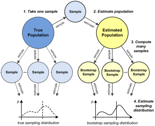
Figure 3: The bootstrap method, adapted from lecture notes at the Pennsylvania State University, see https://online.stat.psu.edu/stat555/node/119/, accessed 26 November 2021.

3.2 Bootstrap Framework for Measuring Generalization

We now apply the bootstrap method to estimate generalization of candidate models for representing some system, supposing that for every model the corresponding system is known, and seeking measures of the form ${{gen}:{\mathcal{M}\times\mathcal{S}}\rightarrow{{\left[0,1\right]}}}$. The better $M$ represents $S$, the higher is ${\mathit{gen}_{\!}\left({M,S}\right)}$; with ${\mathit{gen}_{\!}\left({M,S}\right)}=1$ arising if every new trace from $S$ is described by $M$. Conversely, ${\mathit{gen}_{\!}\left({M,S}\right)}=0$ is the worst possible generalization, arising when none of the new distinct traces observed from $S$ are captured by $M$.

As the system is not known, it cannot be measured directly. We thus propose assessing log-based generalization via an estimator function:

$${{gen^{*}}:{\mathcal{M}\times\mathcal{L}\times\mathbb{LSM}\times\mathbb{N}\times\mathbb{N}}\rightarrow{{\left[0,1\right]}}}\,,\vspace*{-0.8ex}$$ (1)

where $\mathbb{LSM}$ is a collection of log sampling methods, with each $\mathit{lsm}\in\mathbb{LSM}$ a randomizing function that, given an event log $L$ and an integer $n$, produces a sample log $L^{*}={\mathit{lsm}_{\!}\left({L,n}\right)}$ from $L$ of size $n$. Given a model $M$, a log $L$, a log sampling method $\mathit{lsm}$, a log sample size $n$, and a log sample count $m$, Algorithm 1 implements the estimator:

$${\mathit{gen^{*}}_{\!}\left({M,L,\mathit{lsm},n,m}\right)}={\mathit{\text{BootstrapGeneralization}}_{\!}\left({M,L,\mathit{gen},\mathit{lsm},n,m}\right)}\,.\vspace*{-0.8ex}$$ (2)

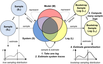
Figure 4: Bootstrapping generalization.

Figure 4 adapts Fig. 3, summarizing the input, output, and computation of Algorithm 1. The four generic stages introduced above are handled in Algorithm 1 as follows:

1. Take one log of the system, as a sample of all the traces the system can generate.

2. Estimate system traces based on that single log.

3. Compute many samples from the estimated system traces.

4. Estimate generalization based on all those sample logs.

Input: Model $M\in\mathcal{M}$, log $L\in\mathcal{L}$, generalization measure ${{gen}:{\mathcal{M}\times\mathcal{S}}\rightarrow{{\left[0,1\right]}}}$, log sampling method $\mathit{lsm}\in\mathbb{LSM}$, sample size $n\in\mathbb{N}$, and number of samples $m\in\mathbb{N}$

Output: Estimated generalization of $M$ with respect to the system that generated $L$

1 $\mathit{data}=[]$

2 for $i\in{\left[1\,..\,m\right]}$ do

3       sample $L_{i}^{*}$ of size $n$ from $L$ using $\mathit{lsm}$, i.e., $L_{i}^{*}={\mathit{lsm}_{\!}\left({L,n}\right)}$

4       $\mathit{data}=\mathit{data}\uplus[{\mathit{gen}_{\!}\left({M\mathchar 44\relax\penalty 0L_{i}^{*}}\right)}]$

5      

6return ${\mathit{average}_{\!}\left({data}\right)}$

Algorithm 1 BootstrapGeneralization($M,L,\mathit{gen},\mathit{lsm},n,m$)

That is, given a log $L$ (Step 1), we use $L$ itself to define the estimated system traces (Step 2). This decision is defensible: $L$ is a record of the system over an extended period, and, more to the point, nothing else is known in the scenario considered. Step 3 appears as line 3 of Algorithm 1, with replicate logs computed using the sampling method $\mathit{lsm}$. Next, lines 4 and 5 of Algorithm 1 implement Step 4 of the generic pattern, with an estimate of the generalization measurement computed for each sample log. Once the individual measurements are collected, aggregation (bagging) takes place at line 5. As shown, the arithmetic mean is returned, but other statistics can also be computed, including confidence intervals, variance, and skewness.

3.3 Log Sampling

We next present two log sampling methods, that is, $\mathit{lsm}$ candidates, suitable for use in Step 2 of the generic bootstrap scheme described in Section 3.1.

There are two main forms of bootstrapping [11]. Nonparametric bootstrapping draws samples from the data using a “with replacement” methodology. The alternative, the parametric bootstrap, generates samples using a known distribution based on parameters estimated from the data. Nonparametric methods reuse elements from the original sample, and hence are only effective if the original sample is a good estimate of the true population. Moreover, the very essence of generalization is to measure the model’s ability to handle hitherto-unseen traces. But nor is it clear what distribution of traces might be employed in a parametric bootstrap for process discovery. The first of the two log sampling techniques we explore is nonparametric. Let $L$ be a log, a multiset of traces, and ${\mathit{randTrace}_{\!}\left({L}\right)}$, a function that returns a randomly selected trace from $L$, each chosen with probability $1/|L|$. Algorithm 2 describes log sampling with replacement.

Input: Log $L$, as a multiset of traces, and sample log size $n\in\mathbb{N}$

Output: Sample log $L^{\prime}$

1 $L^{\prime}=[]$

2 for $i=1$ to $n$ do $L^{\prime}=L^{\prime}\,\uplus\,[{\mathit{randTrace}_{\!}\left({L}\right)}]$

return $L^{\prime}$

Algorithm 2 LogSamplingWithReplacement($L,n$)

The second method we make use of is a semiparametric bootstrap, extending ideas from Theis and Darabi [24] (see Section 5). The semiparametric bootstrap assumes that the true population consists of elements similar but not necessarily identical to those in the sample; another interpretation is that a semiparametric sample is a nonparametric sample containing a certain amount of “noise.” In our context, the noise is in the form of new traces; to create them, we employ a genetic crossover operator, also used in evolutionary computation. Two compatible parent traces generate two offspring if they contain a common subtrace of some minimum length that can become a crossover point.

Let ${\mathit{subseq}_{\!}\left({t,p,n}\right)}$ denote the subtrace of trace $t\in{{\Lambda}^{*}}$ of length $n\in\mathbb{N}$ that starts at position $p\in\mathbb{N}$ in $t$, with $p+n-1\leq\left|{t}\right|$; and let $\left(t\mathchar 44\relax\penalty 0p\mathchar 44\relax\penalty 0n\right)$ identify that subtrace of $t$. For example, $\left(\texttt{abbbcf}\mathchar 44\relax\penalty 02\mathchar 44\relax\penalty 02\right)$ identifies subtrace bb. We also sometimes use underlining as a shorthand, so that $\texttt{a\text@underline{bb}bcf}=(\texttt{abbbcf},2,2)$. In addition, ${\mathit{prefix}_{\!}\left({t,x}\right)}$ is the prefix of $t$ up to and including the $x$ th action, and ${\mathit{suffix}_{\!}\left({t,x}\right)}$ is the suffix of $t$ from and including that $x$ th action. For example, ${\mathit{prefix}_{\!}\left({\texttt{trace},3}\right)}=\texttt{tra}$ and ${\mathit{suffix}_{\!}\left({\texttt{trace},3}\right)}=\texttt{ace}$.

Input: Traces $t_{1},t_{2}\in{{\Lambda}^{*}}$ and length of common subtrace $k\in\mathbb{N}$

Output: Set of all breeding sites for $t_{1}$ and $t_{2}$ for common subtraces of length $k$

1 $\mathit{sites}=\left\{\right\}$

2 for $p_{1}=1$ to $\left|{t_{1}}\right|-k+1$ do

3       for $p_{2}=1$ to $\left|{t_{2}}\right|-k+1$ do

4             if ${\mathit{subseq}_{\!}\left({t_{1},p_{1},k}\right)}={\mathit{subseq}_{\!}\left({t_{2},p_{2},k}\right)}$ then

5                   $\mathit{sites}=\mathit{sites}\cup\left\{(p_{1}\mathchar 44\relax\penalty 0p_{2})\right\}$

6                  

7            

8      

9return $\mathit{sites}$

Algorithm 3 BreedingSites($t_{1},t_{2},k$)

Suppose that traces $t_{1}$ and $t_{2}$ share $k$ actions, $(t_{1},p_{1},k)=(t_{2},p_{2},k)$, and that $\circ$ is a concatenation operator. Then, the crossover operator $\otimes$ creates a new trace by joining $t_{1}$ and $t_{2}$ across that common subtrace: $\left(t_{1}\mathchar 44\relax\penalty 0p_{1}\mathchar 44\relax\penalty 0k\right)\,\otimes\,\left(t_{2}\mathchar 44\relax\penalty 0p_{2}\mathchar 44\relax\penalty 0k\right)\,=\,{\mathit{prefix}_{\!}\left({t_{1},p_{1}+k-1}\right)}\circ{\mathit{suffix}_{\!}\left({t_{2},p_{2}+k}\right)}$. For example, traces abbcf and abbbbcf are obtained from abbbcf via self-crossover, with bb appearing at the breeding sites $p_{1}=2$ and $p_{2}=3$, yielding $\texttt{a\text@underline{bb}bcf}\,\otimes\,\texttt{ab\text@underline{bb}cf}\,=\,\texttt{abbcf}$, and $\texttt{ab\text@underline{bb}cf}\,\otimes\,\texttt{a\text@underline{bb}bcf}\,=\,\texttt{abbbbcf}$. Two traces might have multiple breeding sites, with the count determined by the traces and the value of $k$. Algorithm 3 identifies all breeding sites for two input traces. For example, adeef and adefabcfadef have six $k=2$ breeding sites: $\left\{\left(1\mathchar 44\relax\penalty 01\right)\mathchar 44\relax\penalty 0\left(1\mathchar 44\relax\penalty 09\right)\mathchar 44\relax\penalty 0\left(2\mathchar 44\relax\penalty 02\right)\mathchar 44\relax\penalty 0\left(2\mathchar 44\relax\penalty 010\right)\mathchar 44\relax\penalty 0\left(4\mathchar 44\relax\penalty 03\right)\mathchar 44\relax\penalty 0\left(4\mathchar 44\relax\penalty 011\right)\right\}$.

Input: Logs $L_{1}$ and $L_{2}$, as multisets of traces, length of common subtrace $k\in\mathbb{N}$, and breeding probability $p\in{\left[0,1\right]}$

Output: Log $L^{\prime}$ of traces that result from breeding $L_{1}$ and $L_{2}$

1 $L^{\prime}=[]$

2 for $i=1$ to $\lceil{\left|{L_{1}}\right|}/{2}\rceil$ do

3       $t_{1}={\mathit{randTrace}_{\!}\left({L_{1}}\right)}$

4       $t_{2}={\mathit{randTrace}_{\!}\left({L_{2}}\right)}$

5       $\mathit{sites}={\mathit{\text{BreedingSites}}_{\!}\left({t_{1},t_{2},k}\right)}$

6       if ${\mathit{rand}_{\!}\left({}\right)}<p$ and $\mathit{sites}\neq[]$ then

7             select a random pair $(p_{1},p_{2})$ from $\mathit{sites}$

8             $L^{\prime}=L^{\prime}\,\uplus[\left(t_{1}\mathchar 44\relax\penalty 0p_{1}\mathchar 44\relax\penalty 0k\right)\otimes\left(t_{2}\mathchar 44\relax\penalty 0p_{2}\mathchar 44\relax\penalty 0k\right)\mathchar 44\relax\penalty 0\left(t_{2}\mathchar 44\relax\penalty 0p_{2}\mathchar 44\relax\penalty 0k\right)\otimes\left(t_{1}\mathchar 44\relax\penalty 0p_{1}\mathchar 44\relax\penalty 0k\right)]$

9            

10      else

11             $L^{\prime}=L^{\prime}\,\uplus[t_{1}\mathchar 44\relax\penalty 0t_{2}]$

12            

13      

return $L^{\prime}$

Algorithm 4 LogBreeding($L_{1},L_{2},k,p$)

In terms of a system or model, each possible candidate crossover site represents a “hyper jump” between pairs of states that share a common $k$-action context. We do not claim that all systems actually behave in this way; but 3.2, below, shows that some interesting classes of systems do. A noteworthy property of the crossover operator is that it allows loops to be inferred if traces that include the loop appear in the log. For example, in Fig. 1b, the state labeled b is the location of a loop of length one, with both of ab and bb as $k=2$ contexts; and, as already noted, the crossover operator can spawn both abbcf and abbbbcf if abbbcf is available in the log.

Input: Log $L$, a multiset of traces, and sample log size $n\in\mathbb{N}$. The number of log generations $g\in\mathbb{N}$, the common subtrace length $k\in\mathbb{N}$, and the breeding probability $p\in{\left[0,1\right]}$ are assumed to be constants

Output: Sample log $L^{\prime}$

1 $G[0]=L$

2 for $i=1$ to $g$ do $G[i]={\mathit{\text{LogBreeding}}_{\!}\left({L,G[i-1],k,p}\right)}$

3 $L^{\prime}={\mathit{\text{LogSamplingWithReplacement}}_{\!}\left({\cup_{i=0}^{g}{G[i]},n}\right)}$

4 return $L^{\prime}$

Algorithm 5 LogSamplingWithBreeding($L,n$)

Algorithms 4 and 5 crystallize these ideas, assuming that ${\mathit{rand}_{\!}\left({}\right)}$ returns a uniformly distributed value in ${\left[0,1\right]}$. In Algorithm 4, traces are chosen from each of $L_{1}$ and $L_{2}$, and then, with some probability $p$, checked for $k$-overlaps, and permitted to breed. If they do breed, their offspring are added to the output set; if they do not, the strings themselves are added. That process iterates until $L^{\prime}$ contains $\approx|L_{1}|$ traces. Algorithm 5 then adds the notion of generations, with the output log $L^{\prime}$ of size $n$ a random selection across traces formed during $g$ generations of breeding, where the $i$ th generation arises when the original log $L$ is bred with the $i-1$ th generation. Algorithm 5 thus provides a semiparametric $\mathit{lms}$ sampler that can, like Algorithm 2, be used for bootstrapping.

3.4 Generalization Measures

We now present two measures that quantify the ability of a model to represent a system.

As noted in Section 2.3, Buijs et al. [7] suggest that model-system recall be used to measure generalization. However, that proposal has two limitations. First, the measure is of only limited utility when models can describe infinite collections of traces, as cardinality measures over sets become problematic. Second, given a model $M$ and system $S$, but where $M\not\subseteq S$, the suggested calculation is indeterminate. The first limitation can be resolved by replacing the cardinality measure over sets with ${\mathit{ent}_{\!}\left({\cdot}\right)}$, a measure inspired by the topological entropy of a potentially infinite language [22]. The result is a measure referred to as the coverage of $M$ with $S$, and, in essence, is the model-system recall instantiated with the entropy as an estimation of cardinality:

$${\mathit{ModelSystemRecall}_{\!}\left({M,S}\right)}=\frac{{\mathit{ent}_{\!}\left({M\cap S}\right)}}{{\mathit{ent}_{\!}\left({M}\right)}}\,.\vspace*{-0.8ex}$$ (3)

By analogy, we now suggest addressing the second limitation by considering model-system precision as a second aspect that characterizes the generalization of the model:

$${\mathit{ModelSystemPrecision}_{\!}\left({M,S}\right)}=\frac{{\mathit{ent}_{\!}\left({M\cap S}\right)}}{{\mathit{ent}_{\!}\left({S}\right)}}.\vspace*{-0.8ex}$$ (4)

Model-system precision and recall can both be reported, or a single blended value – their harmonic mean, for example – can be computed. We postpone discussion of which approach is preferable to future work. The entropy-based model-log measures of precision and recall satisfy all the desired properties for the corresponding class of measures [23], making it interesting to study how these measures perform, in terms of generalization properties [2], when comparing the traces of the model and system.

3.5 Consistency

Next, we show that our estimator of generalization is consistent for systems captured as DFGs, which are graphs of actions commonly used by industry to describe process models [1], making it reasonable to assume that the unknown systems they correspond to are also captured as DFGs. Figure 1 shows two DFGs.

Definition 3.1 (DFG)

A directly-follows graph (DFG) is a tuple $(\Phi,\Psi,\phi,\psi,i,o)$; with $\Phi\subseteq{\Lambda}$ a set of actions; $\Psi\subseteq((\Phi\times\Phi)\cup(\left\{i\right\}\times\Phi)\cup(\Phi\times\left\{o\right\}))$ a directly-follows relation; ${{\phi}:{\Phi\cup\left\{i\mathchar 44\relax\penalty 0o\right\}}\rightarrow{\mathbb{N}_{0}}}$ an action frequency function; ${{\psi}:{\Psi}\rightarrow{\mathbb{N}_{0}}}$ an arc frequency function; and $i\not\in{\Lambda}$ and $o\not\in{\Lambda}$ the input and the output of the graph. $\lrcorner$

We define the semantics of a DFG via a mapping to a finite automaton [20].

Definition 3.2 (DFA)

A deterministic finite automaton (DFA) is a tuple $\left(Q\mathchar 44\relax\penalty 0{\Lambda}\mathchar 44\relax\penalty 0\delta\mathchar 44\relax\penalty 0q_{0}\mathchar 44\relax\penalty 0A\right)$, with $Q$ a finite set of states; ${\Lambda}$ a finite set of actions; ${{\delta}:{Q\times{\Lambda}}\rightarrow{}}$ $Q$ the transition function; $q_{0}\in Q$ the start state; and $A\subseteq Q$ is the set of accepting states. $\lrcorner$

A sequence of actions is a trace of a DFA if the DFA accepts that sequence of actions. A DFA is stable if $\forall(q_{1},\lambda,q_{2})\in\delta\wedge\forall(q^{\prime}_{1},\lambda^{\prime},q^{\prime}_{2})\in\delta:((\lambda=\lambda^{\prime})\Rightarrow(q_{2}=q^{\prime}_{2}))$. A DFG $(\Phi,\Psi,\phi,\psi,i,o)$ gives rise to a DFA $(\Phi\cup\left\{i\mathchar 44\relax\penalty 0o\right\},\Phi\cup\left\{o\right\},\delta,i,o)$, with $\delta=\{(s,t,t)\in(\left\{i\right\}\cup\Phi)\times(\Phi\cup\left\{o\right\})\times(\Phi\cup\left\{o\right\})\mid(s,t)\in\Psi\}$ that is guaranteed to be stable.

Lemma 3.1 (Stable DFAs)

A DFA of a DFG is stable. $\lrcorner$

Indeed, an occurrence of an action is always followed by the same opportunities for future actions; and hence, any offspring that result from the crossover of two traces of a stable DFA are also traces of the DFA.

Lemma 3.2 (Trace crossover)

If $t_{1},t_{2}\in{{\Lambda}^{*}}$ are traces of a stable DFA and if $t=(t_{1},p_{1},1)\otimes(t_{2},p_{2},1)$, for $p_{1},p_{2}\in\mathbb{N}$, then $t$ is accepted by the DFA. $\lrcorner$

Proof sketch. By definition, $t={\mathit{prefix}_{\!}\left({t_{1},p_{1}}\right)}\circ{\mathit{suffix}_{\!}\left({t_{2},p_{2}+1}\right)}$, and hence the elements in $t_{1}$ and $t_{2}$ at positions $p_{1}$ and $p_{2}$ are instances of the same action. As the DFA is stable, ${\mathit{prefix}_{\!}\left({t_{1},p_{1}}\right)}$ and ${\mathit{prefix}_{\!}\left({t_{2},p_{2}}\right)}$ lead to the same state $q$ in the DFA; and because ${\mathit{suffix}_{\!}\left({t_{2},p_{2}+1}\right)}$ leads from $q$ to an accept state, $t$ must also be accepted by the DFA. $\blacksquare$

If two traces share a crossover of any length, there must also be a crossover of length one that results in the same offspring pair. Consequently, a log sample that results from Algorithm 5 for an input log composed of traces from a system that is a DFG will also contain valid traces. Such a log sample estimates the system at least as well as the original log. One further condition is then sufficient to allow our main result.

Theorem 3.1 (Bootstrapping DFAs)

Let $L$ be a set of traces from a stable DFA describing a language $L^{*}$, $L\subseteq L^{*}$, such that each subtrace of length two of any trace in $L^{*}$ is also a subtrace of some trace in $L$. Then $L^{\prime}$ is a log of the DFA with $L\subseteq L^{\prime}$ and $L^{\prime}\subseteq L^{*}$ iff $L^{\prime}$ can result from log sampling with breeding (Algorithm 5) for input log $L$ and common subtrace length $k=1$. $\lrcorner$

Proof sketch. ($\Rightarrow$) If $t\in L^{\prime}$ is not a crossover of two sequences in $L^{\prime}$ then $t$ is a trace of the DFA (base case). Otherwise, let $t=(t_{1},p_{1},1)\otimes(t_{2},p_{2},1)$, where $t_{1}$ and $t_{2}$ are traces of the DFA. As the DFA is stable, $t$ is a trace of the DFA, and the action at position $p_{1}+1$ in $t$ is taken from the state of the DFA reached after the action at position $p_{1}$.
($\Leftarrow$) Let $t\in L^{\prime}$, and consider two cases. (i) If $t\in L$, then $t$ is a trace of the DFA. (ii) Suppose $t\not\in L$. But ${\mathit{prefix}_{\!}\left({t,0}\right)}$ is a computation of the DFA, and if ${\mathit{prefix}_{\!}\left({t,k}\right)}$, $k<\left|{t}\right|$ is a computation of the DFA, then ${\mathit{prefix}_{\!}\left({t,k+1}\right)}$ is also computation of the DFA, via two subcases. (ii.a) If $t=(t_{1},k,1)\otimes(t_{2},m,1)$, $m\in\mathbb{N}$, $t_{1},t_{2}\in L^{\prime}$ it follows (the DFA is stable) that ${\mathit{prefix}_{\!}\left({t,k+1}\right)}$ is a computation of the DFA. Indeed, $t_{1}$ and $t_{2}$ are traces of the DFA, shown by structural induction on the hierarchy of crossovers over the sequences in $L^{\prime}$, and the last action in the prefix is taken from the same state of the DFA. (ii.b) Otherwise, ${\mathit{prefix}_{\!}\left({t,k+1}\right)}$ is a prefix of some trace of the DFA and, thus, is its computation, implying that $t$ leads to an accept state, as its last action is the last action of some trace in $L$. $\blacksquare$

Hence, the larger the bootstrapped samples of a DFG log that are generated, the better the estimate of the system – meaning that bootstrap generalization (Algorithm 1) instantiated with the entropy-based model-system measures (Eqs. 3 and 4) is consistent, a consequence of the monotonicity property of the two model-system measures [22].

3.6 Example

Consider again the running example of Section 2.2. For the languages $M$ and $S$ described by the DFGs of Fig. 1a and Fig. 1b, ${\mathit{ModelSystemRecall}_{\!}\left({M,S}\right)}=$0.867$$ and ${\mathit{ModelSystemPrecision}_{\!}\left({M,S}\right)}=$0.867$$, noting that precision and recall are the same if the complexity of the system and model languages is the same [22].

Assuming now that $S$ is unknown, we apply Algorithm 1 (BootstrapGeneralization) to estimate the corresponding measurements, with parameters: input model $M$; the log $L$ of 66 traces presented in Section 2.2; the generalization measures of Eqs. 3 and 4 ($\mathit{gen}$); log sampling with breeding as described by Algorithm 5 ($\mathit{lsm}$); sample log sizes of $n=$100,000$$ and $1,000,000$ traces; $m=$100$$ log replicates; $g=$10,000$$ log generations; breeding sites of length $k=2$; and a breeding probability of $p=$1.0$$. The estimation process yielded model-system precision and recall measurements of $0.892,209$ and $0.912,492$ (for $n=$100,000$$), and of $0.897,187$ and $0.908,485$ ($n=$1,000,000$$). In contrast, the original log $L$ of 66 traces does not provide a good representation of the system, with model-log precision and recall of $0.791$ and $0.935$, respectively. The two computations took $457$ and $575$ seconds, respectively, on a commodity laptop running Windows 10, Intel(R) Core(TM) i7-7500U CPU @ 2.70GhZ and 16GB of RAM.

Table 1: Precision and recall estimates via bootstrapping, plus the number of distinct traces per replica, together with 95% confidence intervals, using $m=$100$$ replicates throughout: (a) varying $n$, the number of traces per replicate, with $g=$10,000$$ generations held constant; and (b) varying $g$, with $n=$10,000$$ held constant. The confidence intervals for precision and recall are for the estimated values considering the input parameters and, thus, might not include the true values.

(a)

(b)

$n$ precision recall traces $100$ $0.834,565,956,1$$\,\pm\,$ $0.001,339,3$ $0.951,812,634,8$$\,\pm\,$ $0.002,302,2$ $11.91$$\,\pm\,$ $0.324,987,4$ $1000$ $0.862,678,670,8$$\,\pm\,$ $0.001,233,0$ $0.929,885,483,1$$\,\pm\,$ $0.001,855,4$ $27.69$$\,\pm\,$ $0.608,227,1$ $10,000$ $0.881,427,795,9$$\,\pm\,$ $0.000,762,9$ $0.918,732,150,0$$\,\pm\,$ $0.000,701,0$ $56.54$$\,\pm\,$ $0.742,511,3$ $100,000$ $0.892,209,258,0$$\,\pm\,$ $0.000,387,4$ $0.912,491,649,6$$\,\pm\,$ $0.000,498,9$ $107.30$$\,\pm\,$ $1.030,923,7$ $1,000,000$ $0.897,186,714,8$$\,\pm\,$ $0.000,273,8$ $0.908,484,670,2$$\,\pm\,$ $0.000,334,9$ $166.22$$\,\pm\,$ $1.375,104,9$

$g$ precision recall traces $100$ $0.872,070,763,1$$\,\pm\,$ $0.001,098,6$ $0.920,608,855,4$$\,\pm\,$ $0.000,908,2$ $41.62$$\,\pm\,$ $0.810,645,1$ $1000$ $0.880,237,156,2$$\,\pm\,$ $0.000,827,4$ $0.919,267,825,1$$\,\pm\,$ $0.000,666,9$ $53.66$$\,\pm\,$ $0.768,600,4$ $10,000$ $0.881,427,795,9$$\,\pm\,$ $0.000,762,9$ $0.918,732,150,0$$\,\pm\,$ $0.000,701,0$ $56.54$$\,\pm\,$ $0.742,511,3$ $100,000$ $0.882,019,485,7$$\,\pm\,$ $0.000,706,5$ $0.919,184,104,4$$\,\pm\,$ $0.000,592,5$ $56.82$$\,\pm\,$ $0.734,609,6$ $1,000,000$ $0.880,745,500,9$$\,\pm\,$ $0.000,694,7$ $0.918,487,962,7$$\,\pm\,$ $0.000,623,2$ $55.90$$\,\pm\,$ $0.691,690,9$

Table 1 shows other values generated by bootstrapping. The simplicity of the example configuration – with just a handful of distinct traces in $L$, and hence a very limited range of $k=2$ breeding sites – means that the number of distinct traces per replicate log grows relatively slowly. However, as the traces of the log contain all the subtraces of length two that can be found in traces in the language of the system it is guaranteed (3.1) that the larger the bootstrapped logs become, the more complete the coverage of the system and, consequently, the more accurate the estimated generalization.

4 Evaluation

4.1 Data and Experimentation

Algorithms 1, 2, 3, 4 and 5 were implemented and used to demonstrate the feasibility of our approach when used in (close to) industrial settings. A set of $60$ DFGs shared with us by Celonis SE (https://www.celonis.com) was then used as a library of ground truth systems [20, 4]. Those reference DFGs were generated from three source logs (Road Traffic Fine Management Process, RTFMP [9], Sepsis Cases [17], and BPI Challenge 2012 [25]); two different discovery techniques (denoted “PE” and “VE”); and ten combinations of parameter settings (denoted “01” to “10”).

For each of the $60$ DFGs, we constructed a log of $100$ traces by taking “random walks” through its states. Commencing at the start vertex, the first context, one action was chosen uniformly randomly from the edges available, and the context switched to the destination of that edge. That process was iterated until the final state of the system was reached as the context (every non-final state in these models has at least one outward edge), thereby generating one trace in the corresponding log.

Next, from each of the $60$ generated logs, we discovered a process model using the Inductive Mining algorithm with a noise threshold of $0.8$ [15]. In this controlled experimental setting, in which all of system ($S$), log ($L$), and discovered model ($M$) are known, we have the ability to compute true model-system precision and recall (Eqs. 4 and 3), that is, the ground truth generalization of the derived model.

Then we “forget” about the ground truth system, and estimate the same measurements using Algorithm 1, invoked on each combination of derived model $M$ and log $L$, in conjunction with: model-system precision and recall measures ($\mathit{gen}$); log sampling with trace breeding (Algorithm 4 as $\mathit{lsm}$); a sample log size of $n=$100,000$$; $m=$50$$ log replicates; $g=$10,000$$ log generations; a common subtrace length of $k=$2$$; and a breeding probability of $p=1.0$. All computation was on a Linux server with Intel(R) Xeon(R) Processor (Cascadelake), $32$ cores @ 2.0GHz each, and $288$GB of memory.

4.2 Results

A subset of results is shown in Table 2, covering twelve systems (three original processes, the “PE” and “VE” discovery mechanisms, and the “04” and “07” parameter settings), with each row showing data for a single ground truth system. The columns “model-system” and “model-log” report true model-system precision and recall and the corresponding model-log values; and the columns “bootstrapped generalization” give estimated model-system precision and recall computed via the new bootstrapping process, together with $95$% confidence intervals. All of the bootstrapped values are closer to the true generalization values than the corresponding model-log values, confirming the applicability of the new approach. For example, in the first row in Table 2 the true value of model-system precision, which as discussed in Section 3.4 is used as a measure of generalization, is $0.60$. The precision between that model and the log is $0.48$, while the bootstrapped precision is equal to $0.55\pm 0.00$, better approximating $0.60$.

Table 2: True model-system precision and recall, model-log precision and recall, and estimated precision and recall via bootstrapping, plus the number of distinct traces per replica, together with 95% confidence intervals, see the text for configuration details.

system				model-system		model-log		bootstrapped generalization
	name	nodes	edges	prec.	recall	prec.	recall	precision		recall		traces
1	PE BPI Chall. 04	$16$	$26$	$0.595,225,8$	$1.000,000,0$	$0.482,108,4$	$0.999,245,4$	$0.552,675,6$$\,\pm\,$	$0.000,323,3$	$0.999,766,2$$\,\pm\,$	$0.000,289,5$	$3540.521,739,1$$\,\pm\,$	$13.480,188,3$
2	PE BPI Chall. 07	$25$	$48$	$0.250,979,4$	$1.000,000,0$	$0.174,866,4$	$0.999,888,6$	$0.194,267,9$$\,\pm\,$	$0.000,103,5$	$1.000,025,6$$\,\pm\,$	$0.000,054,9$	$2488.693,877,6$$\,\pm\,$	$9.969,714,1$
3	VE BPI Chall. 04	$16$	$34$	$0.565,639,6$	$0.999,981,7$	$0.384,059,8$	$1.000,016,4$	$0.464,962,2$$\,\pm\,$	$0.000,113,6$	$0.999,998,1$$\,\pm\,$	$0.000,015,3$	$2383.880,000,0$$\,\pm\,$	$10.489,407,0$
4	VE BPI Chall. 07	$20$	$57$	$0.448,494,4$	$1.000,000,0$	$0.230,620,0$	$0.999,896,3$	$0.281,957,9$$\,\pm\,$	$0.000,162,3$	$0.999,997,2$$\,\pm\,$	$0.000,020,2$	$3088.560,000,0$$\,\pm\,$	$9.543,210,5$
5	PE RTFMP 04	$12$	$24$	$0.442,949,8$	$1.000,000,0$	$0.380,762,3$	$0.999,980,1$	$0.429,444,4$$\,\pm\,$	$0.000,055,1$	$0.999,995,7$$\,\pm\,$	$0.000,008,4$	$921.760,000,0$$\,\pm\,$	$4.338,948,3$
6	PE RTFMP 07	$13$	$54$	$0.456,667,9$	$1.000,000,0$	$0.261,072,5$	$1.000,000,0$	$0.333,058,0$$\,\pm\,$	$0.000,244,0$	$1.000,000,0$$\,\pm\,$	$0.000,000,0$	$2521.200,000,0$$\,\pm\,$	$9.234,398,4$
7	VE RTFMP 04	$10$	$29$	$0.597,082,1$	$1.000,000,0$	$0.398,898,7$	$0.999,999,9$	$0.488,163,3$$\,\pm\,$	$0.000,319,5$	$1.000,000,7$$\,\pm\,$	$0.000,000,6$	$2163.980,000,0$$\,\pm\,$	$9.589,648,4$
8	VE RTFMP 07	$13$	$58$	$0.475,015,8$	$1.000,000,0$	$0.247,776,4$	$0.999,998,9$	$0.333,188,6$$\,\pm\,$	$0.000,188,3$	$1.000,000,0$$\,\pm\,$	$0.000,000,1$	$3860.240,000,0$$\,\pm\,$	$13.325,350,2$
9	PE Sepsis Cas. 04	$15$	$35$	$0.471,245,8$	$1.000,000,0$	$0.228,046,2$	$0.999,819,9$	$0.285,172,6$$\,\pm\,$	$0.000,105,9$	$0.999,670,1$$\,\pm\,$	$0.000,281,5$	$5195.500,000,0$$\,\pm\,$	$12.802,747,5$
10	PE Sepsis Cas. 07	$17$	$64$	$0.705,453,7$	$1.000,000,0$	$0.243,591,0$	$1.000,145,5$	$0.317,074,8$$\,\pm\,$	$0.000,188,8$	$1.000,000,0$$\,\pm\,$	$0.000,000,0$	$5405.580,000,0$$\,\pm\,$	$18.152,659,6$
11	VE Sepsis Cas. 04	$12$	$23$	$0.704,180,9$	$1.000,000,0$	$0.535,089,0$	$1.000,015,0$	$0.582,911,4$$\,\pm\,$	$0.000,215,8$	$1.000,129,5$$\,\pm\,$	$0.000,139,0$	$201.640,000,0$$\,\pm\,$	$1.619,871,3$
12	VE Sepsis Cas. 07	$13$	$53$	$0.658,248,6$	$1.000,000,0$	$0.281,572,9$	$1.000,003,1$	$0.362,255,0$$\,\pm\,$	$0.000,224,4$	$0.999,998,9$$\,\pm\,$	$0.000,003,1$	$4777.000,000,0$$\,\pm\,$	$14.450,555,9$

The complete version of the table is available at http://go.unimelb.edu.au/52gi.

The small systems perform consistently better. This suggests the need for further trace breeding mechanisms that target large systems. For example, the bootstrapped precision for the Sepsis Cases log (discovery technique “VE” and parameter “07”, in row 12) is $0.36\pm 0.00$, which is closer to the true model-system precision than is $0.28$, the model-log precision, but still notably different from $0.66$. Note that in this case the DFG has $53$ edges, twice as many as the example in the first row of the table. Avenues for further work thus include assessing different log sampling mechanisms in terms of their accuracy (sampling traces supported by the system); their velocity (sampling accurate traces quickly); and their stability (sampling traces that lead to consistent measurements). For example, the method used in Table 2 is stable, as evidenced by the small confidence intervals of the estimates, but is slow, in that it requires many generations to breed relatively small numbers of new traces.

4.3 Threats to Validity

Several threats to validity are worth mentioning. Firstly, the discovered models were accepted as ground truth systems. These models were discovered by process mining experts independently, without the involvement of the authors of this paper. Nevertheless, they may not represent actual systems accurately. An obvious next step is thus to extend the experiments to datasets that include both the true system models and also logs induced from them. At the moment, such datasets are not available to the process mining research community. Secondly, the collection of $60$ system models used in the evaluation is not representative of the full spectrum of possible systems; indeed, all of the recall measurements ended up being $1.0$. They also come from a limited set of domains, namely, healthcare, loan application, and road traffic management. Hence, while the results confirm the consistency of the estimation approach shown in Section 3.5, they also demonstrate different behaviors – notably, convergence rates – for different (classes of) systems. Further experiments with real-world and synthetic systems and logs will help to understand such properties better.

5 Related Work

Generalization is perhaps the least-studied quality criterion of discovered process models, with just a small number of measures proposed; we now briefly survey those.

Given a function that maps log events onto states in which they occur, alignment generalization [3] counts the number of visits to each state, and the number of different events that occur in each state. If states are visited often and the number of events observed from them is low, it is unlikely that further events will arise, and generalization is good. van der Aalst et al. [3] also propose different forms of cross-validation methodology, including a “leave one out” approach. The bootstrap method provides more general sample reuse [11], and, as discussed in Section 3.1, estimates the population using the sample, and computes fresh samples from the estimated population, rather than using the single sample to both train the prediction model and to assess the prediction error.

Weighted behavioral generalization [6] measures the ratio of allowed generalizations to the allowed plus disallowed generalizations. Allowed and disallowed generalizations are determined based on “weighted negative events,” which capture the fact that the event cannot occur at some position in a trace. The event weight reflects the likelihood of the event being observed in future traces of the system. The more disallowed generalizations that are identified, the lower the generalization.

Anti-alignment based generalization [10] promotes models that describe traces not in the log, without introducing new states. The underlying intuition is that the log describes a significant share of the state space of the system, and that future system traces may trigger fresh actions from known states, but not fresh states. It is implemented using a leave one out cross-validation strategy and “anti-alignments,” traces from the model that are as different as possible to those in the log.

The adversarial system variant approximation [24] uses the log’s traces to train a sequence generative adversarial network (SGAN) that approximates the distribution of system traces, and then employs a sample of traces induced by the SGAN to represent the system’s behavior. Generalization is then measured using standard approaches. Trained SGANs can also be incorporated into our bootstrap-based method to obtain a parametric bootstrap strategy, an option we will explore in future work.

Other approaches to measuring generalization have also been proposed [2, 7]. However, they are only partially able to analyze models with loops. van der Aalst [2] lists ten properties (including three that are subject to debate) that a generalization measure should satisfy; and it has been shown [2, 23] that existing measures don’t satisfy the seven properties that are agreed [3, 6, 10, 2]. Moreover, Janssenswillen et al. [14] show that existing generalization measures assess different phenomena [3, 7, 6]. As the instantiations of the generalization estimator discussed and evaluated in this work rely on the entropy-based precision and recall measures [22], which were shown to satisfy all the desired properties for the corresponding classes of measures [23], it is interesting to study the properties of our generalization estimators. However, properties of the estimators must be studied in the limit (as the input grows and the estimators converge), which requires adjustments of the original properties. We will do that as future work.

An experiment with synthetic models and simulated logs analyzed whether existing model-log precision and recall, and generalization measures can be used as estimators of model-system precision and recall [13]. The experiment measured model-system and model-log properties, and performed statistical analysis to establish relationships between them. The reported results indicate that using currently available methods, it is “nearly impossible to objectively measure the ability of a model to represent the system.” In our work, instead of relating model-system and model-log measurements, we use the bootstrap method to estimate the entire behavior of the system from its log, and then measure model-system properties using the model and the estimated behavior of the system. Under reasonable assumption, our estimator of generalization is consistent.

Also related to the problem of measuring generalization of a discovered model is establishing the rediscoverability of a process discovery algorithm, that is, identifying conditions under which it constructs a model that is behaviorally equivalent to the system and describes the same set of traces [1]. Such conditions usually address both the class of systems and the class of logs for which rediscoverability can be assured. For example, the Inductive Mining algorithm guarantees rediscoverability for the class of systems that are captured as block-structured process models [18] without duplicate actions and in which it is not possible to start a loop with an activity the same loop can also end with [16]. In contrast to rediscoverability guarantees, we study the problem of measuring how well a discovered model describes an unknown original system.

6 Conclusion

We presented a bootstrap-based approach for estimating the generalization of models discovered from logs, parameterized by a generalization measure defined over known systems, and a log sampling method. An instantiation using entropy-based generalization and log sampling based on $k$-overlap breeding of traces is shown to be consistent for the class of systems captured as DFGs. Thus, the larger the constructed samples and the more samples get bootstrapped, the more accurate the estimation of the generalization is. Our evaluation confirmed the approach’s feasibility in industrial settings.

This work marks a first step in a study of the applicability of bootstrap methods for estimating generalization, and can be extended in several ways. In future work we will seek to develop an unbiased estimator, that is, an estimator with no difference between the expected value of the estimation and the true value of the generalization; to study the consistency of generalization estimators for different classes of systems and identify other useful components for instantiating the bootstrap-based approach for estimating the generalization, including log sampling methods and generalization measures over known systems; and to explore the quality of different bootstrap-based estimators of the generalization to overcome problems associated with noisy logs.

Acknowledgment. Artem Polyvyanyy was in part supported by the Australian Research Council project DP180102839. A presentation of this work from an earlier stage of the research project is available at https://youtu.be/8I-87iGCzNI.

References

- [1] van der Aalst, W.M.P.: Process Mining—Data Science in Action. Springer, sec. edn. (2016)
- [2] van der Aalst, W.M.P.: Relating process models and event logs—21 conformance propositions. In: ATAED. CEUR Workshop Proceedings, vol. 2115. CEUR-WS.org (2018)
- [3] van der Aalst, W.M.P., Adriansyah, A., van Dongen, B.F.: Replaying history on process models for conformance checking and performance analysis. Wiley Interdiscip. Rev. Data Min. Knowl. Discov. 2(2) (2012)
- [4] Alkhammash, H., Polyvyanyy, A., Moffat, A., García-Bañuelos: Discovered Process Models 2020-08 (2020), doi: 10.26188/12814535
- [5] Breiman, L.: Bagging predictors. Mach. Learn. 24(2) (1996)
- [6] vanden Broucke, S.K.L.M., Weerdt, J.D., Vanthienen, J., Baesens, B.: Determining process model precision and generalization with weighted artificial negative events. IEEE Trans. Knowl. Data Eng. 26(8) (2014)
- [7] Buijs, J.C.A.M., van Dongen, B.F., van der Aalst, W.M.P.: Quality dimensions in process discovery: The importance of fitness, precision, generalization and simplicity. Int. J. Coop. Inf. Syst. 23(1) (2014)
- [8] Carmona, J., van Dongen, B.F., Solti, A., Weidlich, M.: Conformance Checking—Relating Processes and Models. Springer (2018)
- [9] De Leoni, M., Mannhardt, F.: Road traffic fine management process (2015), doi: 10.4121/UUID:270FD440-1057-4FB9-89A9-B699B47990F5
- [10] van Dongen, B.F., Carmona, J., Chatain, T.: A unified approach for measuring precision and generalization based on anti-alignments. In: BPM. LNCS, vol. 9850. Springer (2016)
- [11] Efron, B.: The Jackknife, the Bootstrap and Other Resampling Plans. Society for Industrial and Applied Mathematics (1982)
- [12] Efron, B., Tibshirani, R.J.: An Introduction to the Bootstrap. Springer (1993)
- [13] Janssenswillen, G., Depaire, B.: Towards confirmatory process discovery: Making assertions about the underlying system. Bus. Inf. Syst. Eng. 61(6) (2019)
- [14] Janssenswillen, G., Donders, N., Jouck, T., Depaire, B.: A comparative study of existing quality measures for process discovery. Inf. Syst. 71 (2017)
- [15] Leemans, S.J.J., Fahland, D., van der Aalst, W.M.P.: Discovering block-structured process models from event logs—A constructive approach. In: Petri Nets. LNCS, vol. 7927 (2013)
- [16] Leemans, S.J.J., Fahland, D., van der Aalst, W.M.P.: Scalable process discovery and conformance checking. Software and Systems Modeling 17(2) (2018)
- [17] Mannhardt, F.: Sepsis cases – event log (2016), doi: 10.4121/UUID:915D2BFB-7E84-49AD-A286-DC35F063A460
- [18] Polyvyanyy, A.: Structuring Process Models. Ph.D. thesis, University of Potsdam (2012)
- [19] Polyvyanyy, A., Alkhammash, H., Ciccio, C.D., García-Bañuelos, L., Kalenkova, A.A., Leemans, S.J.J., Mendling, J., Moffat, A., Weidlich, M.: Entropia: A family of entropy-based conformance checking measures for process mining. In: ICPM Tool Demonstration Track. CEUR Workshop Proceedings, vol. 2703. CEUR-WS.org (2020)
- [20] Polyvyanyy, A., Moffat, A., García-Bañuelos, L.: An entropic relevance measure for stochastic conformance checking in process mining. In: ICPM. IEEE (2020)
- [21] Polyvyanyy, A., Smirnov, S., Weske, M.: Process model abstraction: A slider approach. In: EDOC. pp. 325–331. IEEE Computer Society (2008)
- [22] Polyvyanyy, A., Solti, A., Weidlich, M., Ciccio, C.D., Mendling, J.: Monotone precision and recall measures for comparing executions and specifications of dynamic systems. ACM Trans. Softw. Eng. Methodol. 29(3) (2020)
- [23] Syring, A.F., Tax, N., van der Aalst, W.M.P.: Evaluating conformance measures in process mining using conformance propositions. ToPNoC XIV (2019)
- [24] Theis, J., Darabi, H.: Adversarial system variant approximation to quantify process model generalization. IEEE Access 8 (2020)
- [25] Van Dongen, B.B.F.: BPI challenge 2012 (2012), doi: 10.4121/UUID:3926DB30-F712-4394-AEBC-75976070E91F
- [26] van der Werf, J.M.E.M., Polyvyanyy, A., van Wensveen, B.R., Brinkhuis, M., Reijers, H.A.: All that glitters is not gold—Towards process discovery techniques with guarantees. In: CAiSE. LNCS, vol. 12751. Springer (2021)