Benchpress: A Scalable and Versatile Workflow for Benchmarking Structure Learning Algorithms

Benchpress: A Scalable and Versatile Workflow for Benchmarking Structure Learning Algorithms for Graphical Models Benchpress: a scalable and versatile workflow for structure learning Describing the relationship between the variables in a study domain and modelling the data generating mechanism is a fundamental problem in many empirical sciences. Probabilistic graphical models are one common approach to tackle the problem. Learning the graphical structure for such models is computationally challenging and a fervent area of current research with a plethora of algorithms being developed. To facilitate the benchmarking of different methods, we present a novel workflow, called for producing scalable, reproducible, and platform-independent benchmarks of structure learning algorithms for probabilistic graphical models. is interfaced via a simple JSON-file, which makes it accessible for all users, while the code is designed in a fully modular fashion to enable researchers to contribute additional methodologies. currently provides an interface to a large number of state-of-the-art algorithms from libraries such as BDgraph, BiDAG, bnlearn, causal-learn, gCastle, GOBNILP, pcalg, r.blip, scikit-learn, TETRAD, and trilearn as well as a variety of methods for data generating models and performance evaluation. Alongside user-defined models and randomly generated datasets, the workflow also includes a number of standard datasets and graphical models from the literature, which may be included in a benchmarking study. We demonstrate the applicability of this workflow for learning Bayesian networks in five typical data scenarios. The source code and documentation is publicly available from https://benchpressdocs.readthedocs.io. reproducibility, scalable benchmarking, probabilistic graphical models reproducibility, scalable benchmarking, probabilistic graphical models Felix L. Rios
Department of Mathematics and Computer Science
University of Basel
Spiegelgasse 1, 4051 Basel, Switzerland
E-mail:

Giusi Moffa
Department of Mathematics and Computer Science
University of Basel
Spiegelgasse 1, 4051 Basel, Switzerland
E-mail:

Jack Kuipers
Department of Biosystems Science and Engineering
ETH Zürich
Mattenstrasse 26, 4058 Basel, Switzerland
E-mail:

1 Introduction

Probabilistic graphical models play a central role in modern statistical data analysis. Their compact and elegant way of visualising and representing complex dependence structures in multivariate probability distributions has shown to be successfully applicable in many scientific domains, ranging from disciplines such as social sciences and image analysis to biology, medical diagnosis and epidemiology (see e.g., Elwert, 2013; Friedman et al., 2000; Friedman, 2004; Moffa et al., 2017; Kuipers et al., 2018, 2019).

One of the main advantages of graphical models is that they provide a tool for experts and researchers from non-statistical fields to easily specify their assumptions in a given problem domain, in a highly transparent way. However, in many realistic situations, the number of variables is either too large to build networks by hand, as it is for example the case in genomic applications, or simply no prior knowledge is available about the relationships between different variables. As a consequence, there has been a growing interest in automated strategies to infer the graph component of a probabilistic graphical model from data, so-called structure learning or causal discovery. For recent reviews of the wide flora of algorithms that have emerged in the last two decades, the reader is referred to Koski and Noble (2012); Kitson et al. (2023).

Since the scientific principle of reproducibility is instrumental for high-quality standards in research, there is an increasing demand to present new algorithms with publicly available source code and datasets (see e.g., Munafò et al., 2017; Lamprecht et al., 2020). With publicly available software we should, in principle, be able to easily compare different methods with respect to their performance in different settings. The reality is that the practical implementation of new approaches displays high levels of heterogeneity in many aspects, which renders comparative studies both challenging and time-consuming. One of the main difficulties is that different algorithms may be implemented in different programming languages, with different dependencies. Different packages may differ with respect to the representation of graphical models, the data formats, and the way they interface to the user, e.g., through the command-line arguments, a configuration file, or a function in a specific programming language. Another complication is that the number of computations increases rapidly in comparison studies, especially when input parameters are altered, which requires parallel computation capabilities and careful bookkeeping to record and organise the results for reporting. As a result, researchers may invest considerable effort in producing benchmarking scripts, and may only be able to implement comprehensive comparisons for a handful of relevant algorithms. To complicate matters further, there is no single well-established metric to evaluate the performance of structure learning algorithms. On the contrary, there is a wide range of different metrics to choose from (see e.g., Tsamardinos et al., 2006; Scutari et al., 2019a; Constantinou et al., 2021) and researchers tend to use only a small selected subset of these to evaluate a new algorithm, typically focusing on those relevant to the problem their algorithm addresses.

When it comes to datasets, there are standard choices commonly used in the literature for benchmarking new algorithms. While desirable to also reduce the researchers’ degrees of freedom in terms of data choices, focusing on a limited set of data may have damaging effects by unintentionally leading to solutions specifically tailored to the data properties, rather than more generally targeting structure learning. Despite the ongoing rapid advances in causal discovery algorithms, there is still a lack of unified approaches for simulating benchmarking data that display realistic features and are easily accessible to the user. A recent effort to address this need aims to use assembly lines’ data for generating semisynthetic manufacturing data with known causal relationships (Göbler et al., 2023). Montagna et al. (2023) focus on data generated from models violating the standard assumptions for causal discovery.

With the problems described above in mind, the objective of this work is to develop a unified framework to facilitate the execution and benchmarking of different algorithms. We present a novel (Köster and Rahmann, 2012) workflow called , which is designed for reproducible, platform-independent, and fully scalable benchmarks of structure learning algorithms. is interfaced via an easy-to-use configuration file in JSON-format (Pezoa et al., 2016), where a benchmark setup is specified in a module-based probabilistic programming style, separating model specification, in terms of graph and corresponding parameters, from algorithm execution and evaluation. enables to seamlessly scale the computations to server, cluster, grid and cloud environments, without any changes in the configuration file. The support for containerized software through e.g., Apptainer (Kurtzer et al., 2017) or Docker (Merkel, 2014) images, together with platform-independent representations of data sets and graphs enables to compare algorithms from different libraries, possibly implemented in different programming languages and with different dependencies. Creating a consensus benchmark setup may mitigate distortions in the performance comparison inadvertently resulting from researchers’ degrees of freedom. At the same time, the possibility of easily designing reproducible benchmarking settings will encourage researchers to conduct more comprehensive comparison studies on different datasets and using different metrics.

is implemented in a modular coding style with functionality for researchers to contribute with additional modules for generating models, structure learning algorithms and evaluating results. In the current publicly released version we have already included 54 algorithm modules from some of the most popular libraries such as BDgraph (Mohammadi and Wit, 2019), BiDAG (Suter et al., 2023), bnlearn (Scutari, 2010), causal-learn (Zheng et al., 2023), gCastle (Zhang et al., 2021), GOBNILP (Cussens, 2020), pcalg (Kalisch et al., 2012), r.blip (Scanagatta et al., 2015), scikit-learn (Pedregosa et al., 2011), TETRAD (Glymour and Scheines, 1986), and trilearn (Olsson et al., 2019) along with models and data sets from the standard literature. See Table 6 in the Appendix for a complete list of the currently available algorithms.

With comparable intent, Constantinou et al. (2020) developed Bayesys, albeit exclusively designed for Bayesian networks, a specific type of probabilistic graphical models (Pearl, 1997). Furthermore Bayesys is a Java implementation only including six algorithms for structure learning at the time of writing. Another tool called causal-compare with a similar purpose to was released as part of the TETRAD project (Ramsey et al., 2020). However, the functionality of causal-compare is restricted to the algorithm implementations in the TETRAD project, representing only a subset of available algorithms from the literature. Overall offers wider scope and usability than currently available alternatives since only requires Docker, without placing any special requirements on the implementation of individual algorithms.

is distributed under the GPL v2.0 License, encouraging its use in both, academic and commercial settings. Source code and documentation are available from https://benchpressdocs.readthedocs.io.

The rest of the paper is structured as follows. Section 2 presents an introduction to graphical models along with some notational conventions. Section 3 provides background on current strategies for structure learning. Section 4 describes the structure of the JSON interface and the modules already available for benchmarking. In Section 5, we show how to use in several typical benchmarking scenarios. Installation and usage guidelines are provided in Section 6, while Section 7 discusses how to add new algorithms to the framework.

2 Probabilistic graphical models

This section provides a brief introduction to graphical models and graph theory, with definitions as in e.g., Diestel (2005); Lauritzen (1996). Let $\Prob$ be a $p$-dimensional distribution and let $Y:=(Y_{i})_{i=1}^{p}$ be a random vector such that $Y\sim\Prob$. Further let $G=(V,E)$ be a graph, where $V=\{Y_{i}\}_{i=1}^{p}$ is the node set and $E$ is the edge set, consisting of ordered pairs of distinct elements of $V$. Then $\Prob$, or alternatively $Y$, is said to be Markov with respect to $G$ if separation, based on some graphical criteria, of two subsets of nodes, $Y_{A}$ and $Y_{B}$, by a third set $Y_{C}$ in $G$ implies their conditional independence in $\Prob$, where $Y_{A}:=(Y_{i})_{i\in A}$. The term probabilistic graphical model or graphical model has been used interchangeably in the literature to refer to either the tuple $(G,\Prob)$ or a collection of distributions $\mathcal{P}_{G}$, usually restricted to some specific parametric family, where every $\Prob^{\prime}\in\mathcal{P}_{G}$ is Markov with respect to $G{}$. In this text, we will use the former meaning. In the case where $\Prob$ is restricted to a specific parametric family, it is usually uniquely determined by some parameter vector $\Theta$, thus either notation may be used.

Assuming $f$ is a density for $\Prob$, conditional independence between the random variables $Y_{A}$ and $Y_{B}$ given $Y_{C}$ is well-defined as $f(y_{A}|y_{B},y_{C})=f(y_{A}|y_{C}),$ where $(y_{A},y_{B},y_{C})\in\mathcal{Y}_{A}\times\mathcal{Y}_{B}\times\mathcal{Y}_{C}$ and $\mathcal{Y}_{A}$ denotes the range of $Y_{A}$. In contrast, node separation may have different definitions depending on the type of graph considered. Typical classes of graphs are: undirected graphs, where edges are specified as unordered tuples and separation of $Y_{A}$ and $Y_{B}$ given $Y_{C}$ means that every path between $Y_{A}$ and $Y_{B}$ must pass $Y_{C}$; directed acyclic graphs (DAGs), where edges are represented as ordered tuples and separation is defined by a concept known as d-separation, see e.g., Pearl (1997). Next follows a brief introduction to the type of graphical models currently implemented in .

Bayesian networks constitute one of the most popular classes of graphical models, referring to distributions that are Markov with respect to a DAG. The conditional independence encoded by the DAG implies that the density can be factorised into local conditional densities, where each node $Y_{i}$ is directly dependent on its parents, $pa(Y_{i})$, as

$$f(y)=\prod_{i=1}^{p}f(y_{i}|pa(y_{i})),$$

where $f(y_{i}|pa(y_{i}))$ denotes the conditional density of $Y_{i}$ given $pa(Y_{i})=pa(y_{i})$. This property is appealing for several reasons. Firstly, the decomposition into local conditional probability distribution provides an intuitive way to express and visualise knowledge about a specific problem domain. In particular, an expert could express a causal mechanism in terms of a DAG, which in turn provides a mathematical language to answer causal queries from non-experimental data (Pearl, 1995). Further, it enables fast computations of conditional and marginal distribution using message-passing algorithms by exploiting the factorisation property in the distribution. However, when the DAG is not used for expressing causal knowledge, the direction of the edges may be misleading since the conditional independencies of a distribution are not uniquely encoded by a single DAG in general but rather by a class of Markov equivalent DAGs, all of which encode the same conditional independence statements. One way to represent a Markov equivalence class is by a completed partially directed acyclic graph (CPDAG, see Chickering, 1995). A CPDAG is a partially directed DAG which can be obtained from a DAG by regarding an edge $(Y_{i},Y_{j})$ as undirected if and only if both directed edges $(Y_{i},Y_{j})$ and $(Y_{j},Y_{i})$ are present in some of the DAGs in the same equivalence class. The CPDAG is also sometimes called the essential graph. An equivalent way to represent the conditional independence statements in a DAG is through the pattern graph. The pattern graph of a DAG is the graph obtained by keeping the directions of the v-structures and regarding the remaining edges as undirected. v-structures are characterised by triples of nodes where the edges of two of the nodes, which should not be neighbours, are pointing to the third.

Markov networks or Markov random fields are another popular class of graphical models, referring to distributions that are Markov with respect to an undirected graph. There is, in general, no decomposition into local densities for the models in this class. However, there exist functions $\{\phi_{C}\}_{C\in\mathcal{C}}$ such that

$$f(y)=\prod_{C\in\mathcal{C}}\phi_{C}(y_{C}),$$

where $\mathcal{C}$ is the set of maximal subgraphs where all nodes are directly connected with each other, usually called cliques, which may be leveraged to calculate marginal distributions efficiently. There is a sub-class of undirected graphs called decomposable (DG) or chordal or triangulated, where each cycle with more than three nodes has a chord, an edge which breaks it. Distributions which are Markov with respect to decomposable graphs are called decomposable and their densities are built by local, clique-specific densities, $\{f_{C}\}_{C\in\mathcal{C}}$ and their marginals so that the joint density factorises as

$$f(y)=\frac{\prod_{C\in\mathcal{C}}f_{C}(y_{C})}{\prod_{S\in\mathcal{S}}f_{S}(y_{S})},$$

where $\mathcal{S}$ is the multi-set of separators in $G$, found e.g., as the intersection of neighboring cliques in a so-called junction tree, built from the cliques in the graph; see e.g., Lauritzen (1996) for details. In general Markov networks and Bayesian networks encode different sets of conditional independence statements, and there are sets which we can represent with one model but not the other. Decomposable graphs represent the intersection of those sets of statements which we can represent by both undirected graphs and DAGs (see e.g., Lauritzen, 1996; Cowell et al., 2003; Koller and Friedman, 2009). The DAGs representing the intersection set are called perfect, meaning that all the parents of each node are connected by an edge. Further characterisations of decomposable graphs are found in e.g., Lauritzen (1996); Cowell et al. (2003) and Duarte and Solus (2021).

3 Structure learning

Structure learning algorithms for Bayesian networks were proved to be NP-hard, even when the number of parents of each node is restricted to two (Chickering et al., 2004). Also, the number of undirected graphs grows as $\mathcal{O}(2^{p^{2}})$ even when restricted to decomposable graphs, making an exhaustive search for a specific graph infeasible (see e.g., Wormald, 1985; Olsson et al., 2022; Hebert-Johnson et al., 2023). Therefore, in practice, we must rely on approximation methods which we can divide into three main categories: constraint-based, score-based, and hybrid algorithms, discussed briefly below.

The seed for the first constraint-based algorithm was planted by Verma and Pearl (1991) in the context of causal Bayesian networks. In line with their work, constraint-based methods employ conditional independence tests among the variables to first estimate an undirected graph by, e.g., starting with the complete graph, and excluding an edge $(Y_{i},Y_{j})$ if there exists some set $Y_{A}$ such that the hypothesis $Y_{i}\perp\!\!\!\perp_{\Prob}Y_{j}\mid Y_{A}$ cannot be rejected according to a suitable test procedure. Such methods tend to be very fast but testing can suffer from large numbers of false negatives, i.e., falsely not including edges when they should be present. Relaxing the significance level of the tests to reduce false negatives can, however, rapidly inflate false positives and runtimes.

Score-based methods on the other hand aim to optimise a global score function defined on the graph space. As a workaround to cope with the immense number of graphs, the search is often limited to certain types of graphs. For example in DAG models, one may restrict the number of parents or combine DAGs into larger and more easily represented classes (e.g., orders and partitions Friedman and Koller, 2003; Kuipers and Moffa, 2017). For decomposable graphs, a possibility is to limit the maximal clique size. Score functions may rely on penalised log-likelihoods or on Bayesian posterior probabilities of graphical structures conditional on the observed data (see e.g., Koller and Friedman, 2009). Besides mere optimisation, Bayesian structure learning also focuses on sampling procedure to provide a finer characterisation of the posterior graph distribution. When an expression for the posterior distribution is available at least up to a normalising constant, we can implement Markov chain Monte Carlo (MCMC) schemes to sample from it, see e.g., Madigan et al. (1995); Giudici and Castelo (2003); Friedman and Koller (2003) for early works and Kuipers and Moffa (2017); Jennings and Corcoran (2018) for more recent strategies. In Gaussian Markov networks, Monte Carlo sampling turns out to be infeasible for larger networks since there is in general no analytic expression for the un-normalised posterior (Atay-Kayis and Massam, 2005). On the other hand, score-based methods such as graphical lasso, rely on the fact that the edges in the graph are revealed from the non-zero pattern of the elements in the precision (inverse covariance) matrix. Optimisation techniques can successfully estimate the $L_{1}$-penalised log-likelihood of the precision matrix, and the graph as a by-product; see Friedman et al. (2008); Meinshausen (2008); Witten et al. (2011). Decomposable models, do possess a closed form expression for the un-normalised graph posterior and most inferential methods built on the representation via undirected graphs focus on Monte Carlo sampling (see e.g., Giudici and Green, 1999; Green and Thomas, 2013; Elmasri, 2017; Olsson et al., 2019) with a few focusing on optimisation (see e.g., Carvalho, 2006; Studenỳ and Cussens, 2017; Rantanen et al., 2017).

Hybrid algorithms typically use constraint-based algorithms as a preliminary step called restrict phase to reduce the search space for a score-based method. A score based-algorithm is then used in the maximise phase (see e.g., Tsamardinos et al., 2003; Scanagatta et al., 2015; Jack Kuipers and Moffa, 2022).

4 Benchpress modules and JSON configuration files

In this section, we describe the modules of and the structure of the JSON (Pezoa et al., 2016) configuration file, which serves as the interface for the user. As is implemented as a workflow, a brief overview of the latter will help to illustrate the overall concept of the tool. is a highly popular workflow management system with a custom Python-based programming language enabling the so-called rules, which build the core of a workflow. Each rule typically comprises four types of fields: the input and output fields, defining the input and output files, respectively, the script and container fields, defining the script for generating the output files based on the input files, and the Docker image used for running the script, respectively.

When requesting an output file from a specific rule, will automatically pattern-match the input files of the rule with the output files of other rules, before executing the script. In this way, will recursively start a chain reaction of executions, where each rule only depends on its ancestors through its input files. Thus, the structure of rule relationships may be represented as a DAG, where an arrow from rule A to rule B indicates that an output file from A matches an input file from B. Each rule lives in an independent Apptainer container and the DAG relationship enables parallel executions. Note that, Apptainer is a container management system which requires fewer operating system privileges than e.g. Docker, making it possible to run on shared servers as opposed to Docker which is usually blocked for security reasons.

has built-in support for reading configuration files in JSON format, passed as an argument to the program. The JSON file provides a simple key-value format which is easy to interpret and modify. This property is heavily exploited by , where the JSON file gives a complete interface for the user, without modifying the rules. When the value of a key is another JSON object or a list, we call it a section.

Figure 1: Flowchart for the architecture describing how the files and sections (sharp rectangles) of the JSON configuration file are related to the modules (rounded rectangles with monospace font style). The different colours pink, blue, and purple indicate modules, files and sections related to data, structure learning, and evaluating results respectively. An arrow from a node A to another node B should be read as “B requires input from A”. Thus, for any node, following the arrows in their opposite directions builds a path of the used modules or files. Dashed arrows indicate that one of the parents is required.

At the highest level, there are two main sections, resources and benchmark_setup, described in Section 4.1 and 4.2, respectively. The resources section contains separate subsections of the available modules for specifying graphs (graph), parameters (parameters), data (data), and algorithms for structure learning (structure_learning_algorithms). Each module, in turn, has a list, where each element is an object defining a parameter setting, identified by a unique id. The benchmark_setup section specifies the data models (data) and evaluation methods (evaluation) a user wishes to consider for analysis. The performance evaluation of structure learning algorithms will depend not only on the chosen metric, but also on the particular graphical model of interest, and it may be measured on different spaces, e.g. CPDAGs, pattern graphs or skeletons, and these options are supported by .

The module objects used in benchmark_setup are defined in resources and referenced by their corresponding id’s. The output files of each module are saved systematically under the results/ directory based on the corresponding objects’ values. An important consequence of this design is that an algorithm run for a specific data set will never have to be rerun, instead, the stored output files are used for the different evaluation modules.

Figure 1 shows a flowchart describing how the files and sections relate to the modules in a JSON configuration file. The notation used on Figure 1 is described in more detail in Section 4. Listings 2 later shows an example of such a configuration file and is described in more detail in Section 5.1.

4.1 Resources section (resources)

Tables 1–3 shows the available modules in the graph, parameters, and data sections. For the modules that stem from existing packages, the names are conventionally prefixed by the name of the package on which they are based. In each of these sections, there are special modules, fixed_graph, fixed_params, and fixed_data, enabling the user to provide graphs, parametrizations, and datasets using files. Note that, already contains several standard Bayesian network models, e.g., those available at the website of bnlearn, including the so-called Bayesian network repository (Friedman et al., 1997). Below is a brief description of the other available modules, for more details, we refer to Appendix B and the online documentation.

For the graph modules, the bdgraph_graphsim module uses the graph.sim function of the BDgraph package (Mohammadi and Wit, 2019) to sample various types of random undirected graphs. The pcalg_randdag module uses the randDAG function of the pcalg package (Kalisch et al., 2012) to sample various types of random DAGs and undirected graphs. The trilearn_bandmat and trilearn_randbandmat modules generate undirected decomposable graphs with a band-structured adjacency matrix of a given and random width, respectively. The trilearn_cta module samples decomposable graphs using the so-called Christmas tree algorithm (CTA) (Olsson et al., 2022).

Method	Graph	Package	Module
Fixed graph	DAG, UG	-	fixed_graph
randDAG	DAG, UG	pcalg	pcalg_randdag
graph.sim function	UG	BDgraph	bdgraph_graphsim
Bandmatrix	DG	trilearn	trilearn_bandmat
CTA	DG	trilearn	trilearn_cta
Random bandmatrix	DG	trilearn	trilearn_rand_bandmat

Table 1: Graph modules.

For the modules in the parameters section, the bdgraph_rgwish module samples the precision matrix of an undirected Gaussian graphical model from the G-Wishart distribution (Dawid and Lauritzen, 1993; Atay-Kayis and Massam, 2005; Lenkoski, 2013). The binary_bn module samples the conditional probability tables of a Bayesian network with only binary variables. The sem_params module samples the weights of a structural equation model (SEM) Gaussian Bayesian network (1). The trilearn_hyper-dir module samples the parameters of a multinomial decomposable graphical model from the Hyper-Dirichlet distribution (Dawid and Lauritzen, 1993). The trilearn_intra-class module specifies the covariance matrix of a Gaussian graph intra-class model.

Method	Graph	Package	Module
Fixed parameters	DAG	-	fixed_params
SEM parameters	DAG	Benchpress	sem_params
Binary BN	DAG	Benchpress	binary_bn
Hyper-Dirichlet	DG	trilearn	trilearn_hyper-dir
Graph intra-class	UG	trilearn	trilearn_intra-class
G-Wishart	UG	BDgraph	bdgraph_rgwish

Table 2: Parameterisation modules.

For the modules in the data section, the iid module is a generic module to draw independent identically distributed (i.i.d.) samples from any of the models built by proper combinations of the graph and parameters modules. The gcastle_iidsim module uses the IIDSimulations function of the gCastle package to draw i.i.d. samples from different types of SEM models.

Method	Graph	Package	Module
Fixed dataset(s)	all	-	fixed_data
gCastle i.i.d. (SEM)	DAG	gCastle	gcastle_iidsim
I.i.d. data	all	various	iid

Table 3: Data modules.

The available modules in the structure_learning_algorithms section are listed in Table 6. For the algorithms demonstrated in the simulation studies in Section 5, we give a short overview in Appendix B.

4.2 Benchmark setup (benchmark_setup)

4.2.1 Data setup section (data)

The data section consists of a list of objects, each containing the id of a graph (graph_id), parameters (parameters_id), data (data_id) module object, and a tuple (seed_range), specifying the range of the random seeds used in the modules. For each seed number $i$ in the specified range, a graph $G_{i}$ is obtained as specified according to graph_id. Given $G_{i}$, the parameters in the model $\Theta_{i}$ are obtained according to parameters_id. A data matrix, $\mathbf{Y}_{i}=(Y_{1:p}^{j})_{j=1}^{n}$, is then sampled from $(G_{i},\Theta_{i})$ according to the model and data_id. When combining modules from the different sections, it is important to ensure that $(G_{i},\Theta_{i})$ is a compatible pair, e.g., if $\Theta_{i}$ represents the parameters of Bayesian network then $G_{i}$ is required to be a DAG.

	$G$	$\Theta$	$\mathbf{Y}$
I	-	-	Fixed
II	Fixed	-	Fixed
III	Fixed	Fixed	Generated
IV	Fixed	Generated	Generated
V	Generated	Generated	Generated

Table 4: Data scenarios.

By using the modules for fixed files, we can build models with increased flexibility. The different data sources provided by can be summarised in five scenarios shown in Table 4. Scenario I is the typical scenario for data analysts, where users provide one or more datasets by hand. Scenario II is similar to Scenario I, where the difference is that in addition, the user provides the true graph underlying the data. This situation arises e.g., when replicating a simulation study from the literature, where both the true graph and the dataset are given. Scenarios III-V are pure benchmarking scenarios, where either all of the graphs, parameters, and data are generated (V), or the graphs (III, IV) and possibly parameters (III) are specified by the user.

Note that, when a filename is used as data_id, since the data is fixed, seed_range should be set to null. However, depending on the evaluation module used, the graph_id could be either null or the filename of the true graph underlying the data. For example, the benchmarks module requires that graph_id set to a proper id for a graph module object, however, it is not a requirement for the adjmat_plots module. When the value of data_id is a directory, the other fields should be set to null.

4.2.2 Evaluation section (evaluation)

Table 5 shows the available modules in the evaluation section. The figures for each module are saved systematically in results/ based on the parameterisation of the module used and copied to results/output/ for easy reference. Further details are provided in Appendix B.

Evaluation	Module
Benchmarks	benchmarks
Pairs plot	ggally_ggpairs
Graph plots	graph_plots
True graph plots	graph_true_plots
True graph properties	graph_true_stats
MCMC auto-correlation	mcmc_autocorr_plots
MCMC mean graphs	mcmc_heatmaps
MCMC trajectories	mcmc_traj_plots

Table 5: Evaluation modules.

The benchmarks module provides timings and comparisons using standard benchmarking metrics. The results are summarised in e.g. box plots and receiver operating characteristic (ROC)-type curves. In addition to the figures produced, the raw data is saved in comma separated values (CSV) files which could be analysed externally. The ggally_ggpairs module uses the ggpairs function of the GGally package (Emerson et al., 2013) to visualise the data in pairwise scatter plots. The graph_plots module plots and saves the estimated graphs and adjacency matrices. If the true graph is available (scenarios II-V in Table 4) it also compares the true to the estimated graphs using the graphviz.compare function from the bnlearn package (Scutari, 2010). The graph_true_plots module plots the true underlying graphs and corresponding adjacency matrices. The graph_true_stats module computes and plots properties of the true underlying graphs. For the MCMC algorithms, the following three special evaluation modules are available. The mcmc_heatmaps module estimates posterior edge probabilities and plots them in heatmaps using the seaborn package (Waskom, 2021). The mcmc_traj_plots module plots the value of a given functional for the graphs in an MCMC trajectory. The currently supported functionals are the number of edges for the graphs and the scores. The mcmc_autocorr_plots module plots the auto-correlation of a functional of the graphs in a MCMC trajectory.

5 Benchpress in practice

We demonstrate the functionalities of with seven examples for benchmarking structure learning algorithms for Bayesian networks. We consider the pure benchmarking setting for both binary and continuous data types as well as a fixed data scenario (Section 5.2). For performance evaluation and visualisation, we use the modules benchmarks, graph_true_stats, ggally_ggpairs, and graph_plots. The title rows of each sub-figure describe the settings for the graph, parameters, data modules, and the number of datasets used.

We use the benchmarks module to show scatter plots of the individual results in terms of ROC type curves, where median $FP/P$ is plotted against the median $TP/P$ and estimated 5%-95% percentiles in ROC type figures (see Appendix A.1 for definitions). Since not all methods support the same test procedures or scores, we have chosen the default settings for some of the algorithms. The parameter values are selected so as to indicate how the performance changes. However, some curves are shorter than would be desired due to range limits for the parameters in the programs used.

For binary data we use the Bayesian Dirichlet likelihood-equivalence (BDe) score (Heckerman et al., 1995) in the score-based methods while varying the equivalent sample size parameter (Silander et al., 2007). The benchmarking setup considers the following score-based algorithms: BOSS (boss-bdeu), GRaSP (grasp-bdeu), HC (hc-bde), Tabu (tabu-bde), ASOBS (asobs-bdeu), GOBNILP (gobnilp-bde), Iterative search (itsearch-bde), and order MCMC with the end space of itsearch-bde as start space (omcmc-bde). Furthermore, we include the constraint-based PC algorithm with the $G^{2}$-test (pc-binCItest) and the hybrid method MMHC (mmhc-bde-mi) with the mutual information test and the BDe score. The varying parameter to draw ROC-type curves for all constraint-based methods is the significance level for the independence tests.

For the continuous datasets, we use two different scores in the score-based methods. The benchmarking setup in this case includes HC (hc-bge), Tabu (tabu-bge), GOBNILP (gobnilp-bge), Iterative search (itsearch-bge), and order MCMC using the end space of itsearch-bge as start space (omcmc-bge) with the Bayesian Gaussian likelihood-equivalence (BGe) score (Geiger and Heckerman, 1994; Geiger et al., 2002; Kuipers et al., 2014), and varying levels of the prior parameter. Furthermore we include the FGES (fges-sem-bic), BOSS (boss-sem-bic), and GRaSP (grasp-sem-bic) with the structural equation model Bayesian information criterion (SEM-BIC) score (Glymour and Scheines, 1986), and varying levels of the penalty discount. We also include the NO TEARS algorithm (notears-l2) with the $L_{2}$ penalty. For constraint-based methods we include the PC algorithm (pc-gaussCItest), dual PC algorithm (dualpc), and MMHC (mmhc-bge-zf) with the Fisher’s z-transformation test of partial correlations (Edwards, 2012) with varying significance levels.

5.1 Comparative study between the PC and the dual PC algorithm

We start with a simple demonstration comparing just two algorithms side-by-side and a small-scale simulation study from data scenario V with the PC and the dual PC algorithms. We consider data from 10 random Bayesian network models $\{(G_{i},\Theta_{i})\}_{i=1}^{10}$, where each graph $G_{i}$ has $p=80$ nodes and is sampled using the pcalg_randdag  module. The parameters $\Theta_{i}$ are sampled from the random linear Gaussian SEM using the sem_params  module (Appendix B.2) with $a=0.25,b=1,\mu=0$ and $\sigma=1$. We draw a standardised dataset $\mathbf{Y}_{i}$ of size $n=300$ from each model using the iid  module. Listing 2 shows the content of the JSON configuration file (paper_pc_vs_dualpc.json) for this study.

⬇

{

"benchmark_setup": {

"data": [

{

"graph_id": "avneighs_p20",

"parameters_id": "SEM",

"data_id": "standardized",

"seed_range": [1, 10]

}

],

"evaluation": {

"benchmarks": {

"filename_prefix": "paper_pc_vs_dualpc/",

"show_seed": false,

"errorbar": true,

"errorbarh": false,

"scatter": true,

"path": true,

"text": false,

"ids": ["pc-gaussCItest", "dualpc"]

},

"graph_true_plots": true,

"graph_true_stats": true,

"ggally_ggpairs": false,

"graph_plots": ["pc-gaussCItest", "dualpc"],

"mcmc_traj_plots": [],

"mcmc_heatmaps": [],

"mcmc_autocorr_plots": []

}

},

"resources": {

"data": {

"iid": [

{

"id": "standardized",

"standardized": true,

"n": 300

}

]

},

"graph": {

"pcalg_randdag": [

{

"id": "avneigs4_p20",

"max_parents": 5,

"n": 20,

"d": 4,

"par1": null,

"par2": null,

"method": "er",

"DAG": true

}

]

},

"parameters": {

"sem_params": [

{

"id": "SEM",

"min": 0.25,

"max": 1

}

]

},

"structure_learning_algorithms": {

"dualpc": [

{

"id": "dualpc",

"alpha": [0.001, 0.05, 0.1],

"skeleton": false,

"pattern_graph": false,

"max_ord": null,

"timeout": null

}

],

"pcalg_pc": [

{

"id": "pc-gaussCItest",

"alpha": [0.001, 0.05, 0.1],

"NAdelete": true,

"mmax": "Inf",

"u2pd": "relaxed",

"skelmethod": "stable",

"conservative": false,

"majrule": false,

"solveconfl": false,

"numCores": 1,

"verbose": false,

"indepTest": "gaussCItest",

"timeout": null

}

]

}

}

}

Figure 2: The JSON configuration file paper_pc_vs_dualpc.json to define a small comparison between the PC and dual PC algorithms.

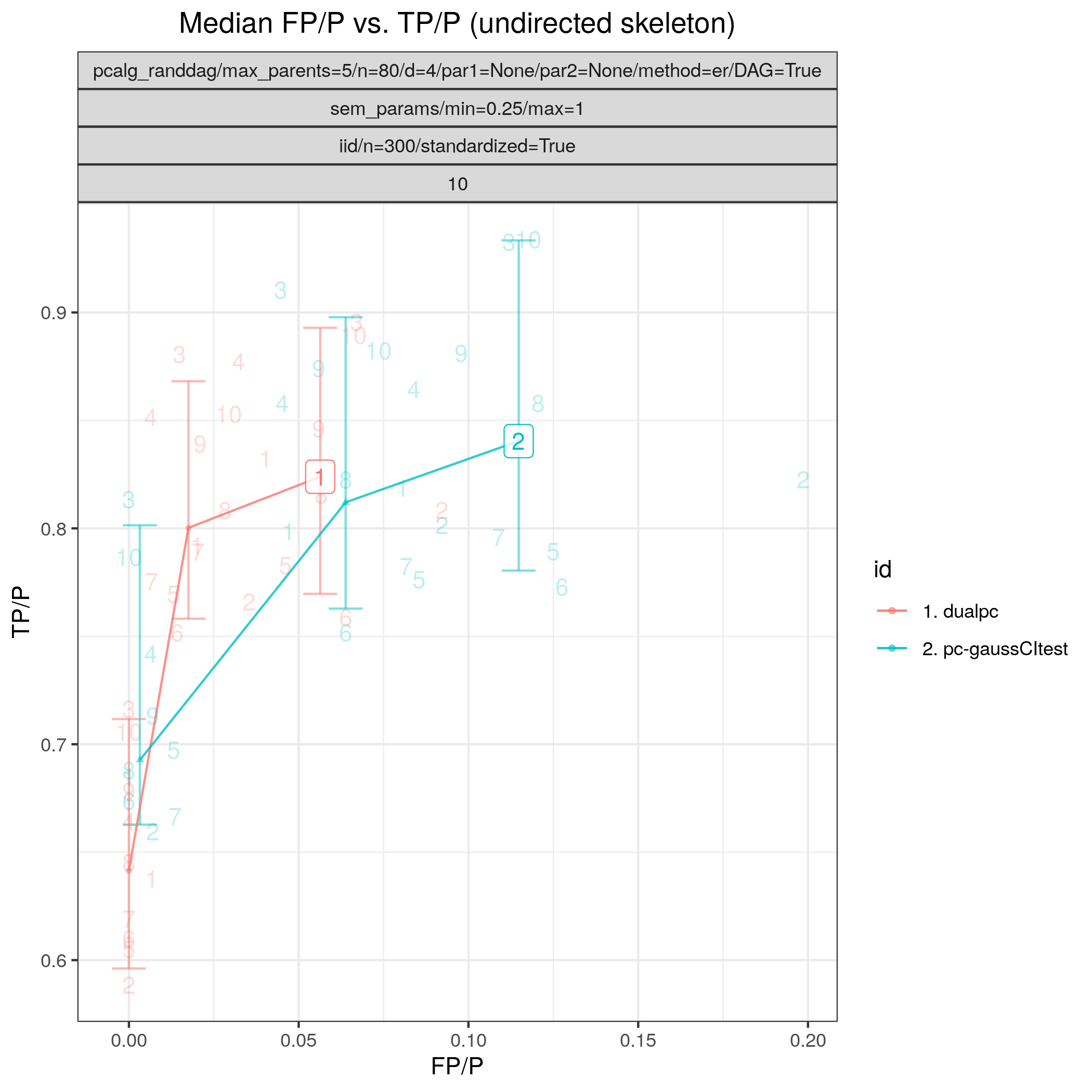
(a)

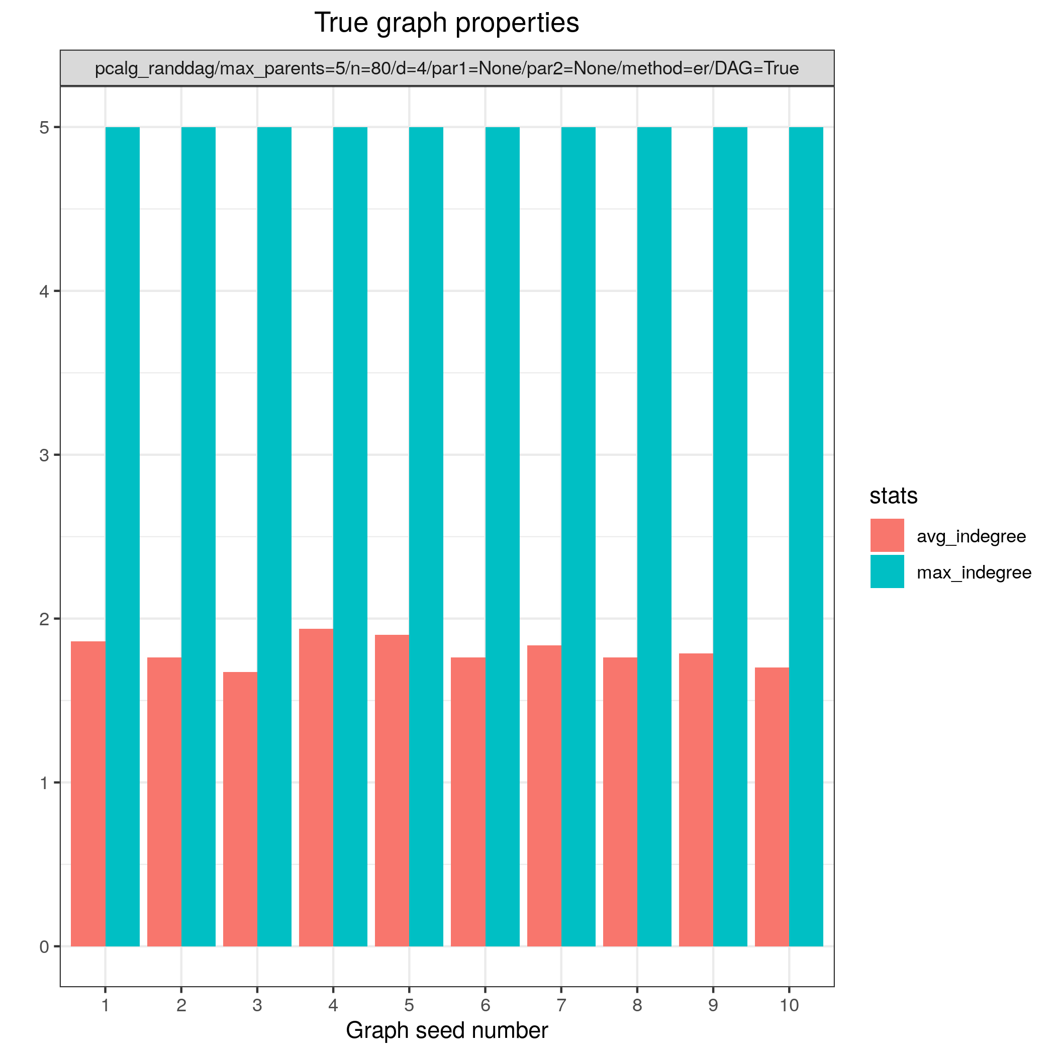
(b)

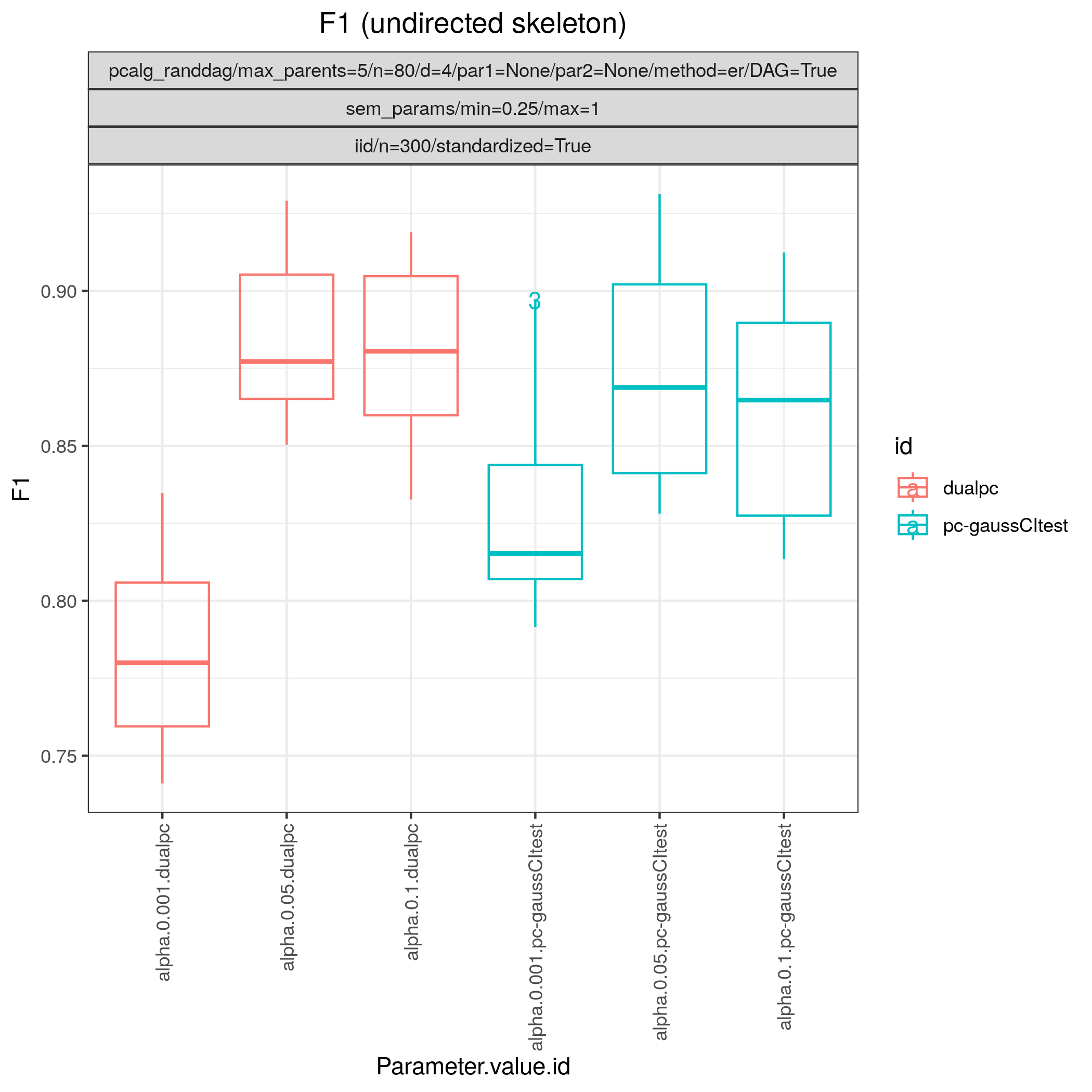
(c)

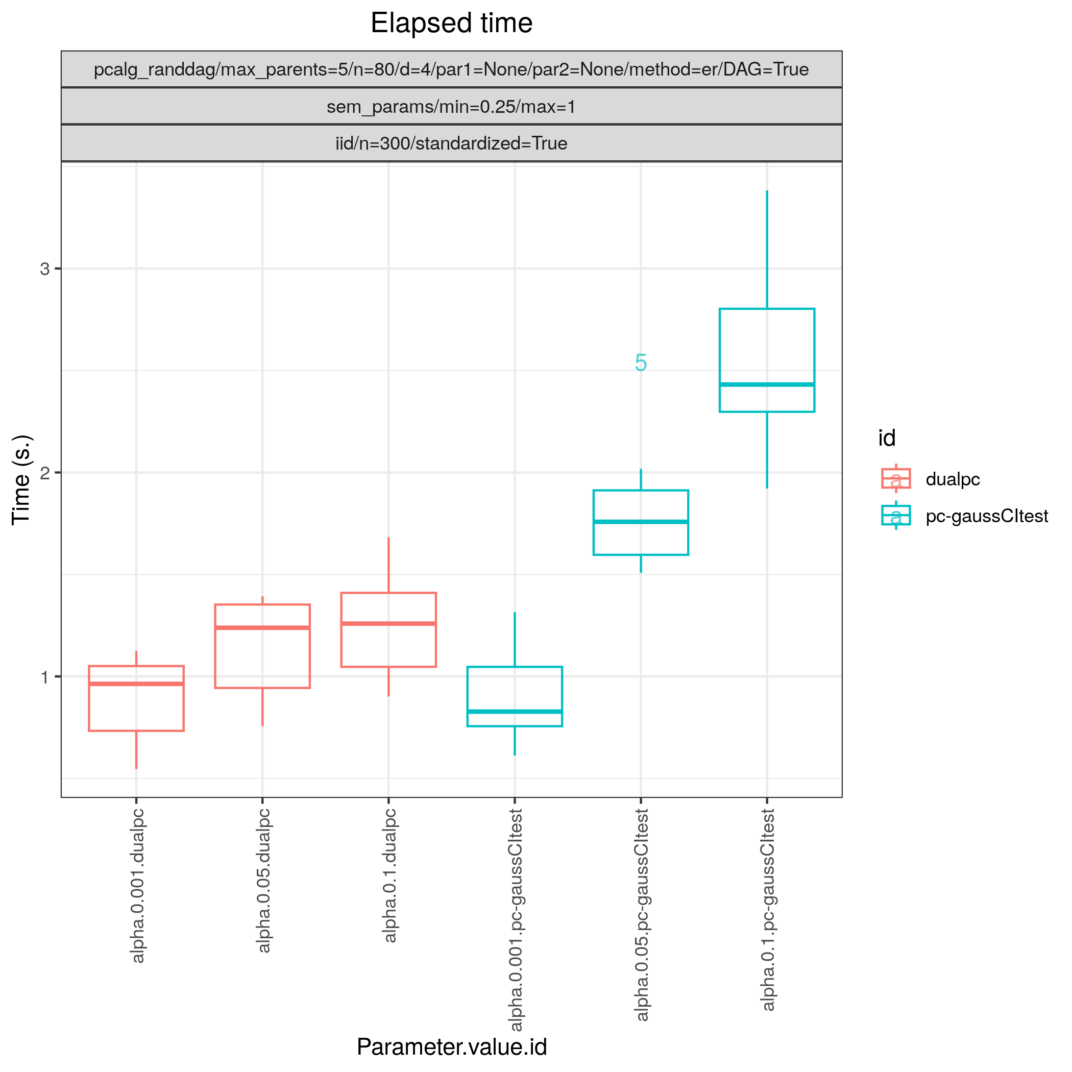
(d)

Figure 3: This figure shows results for a comparative study between the PC pcalg_pc and the dual PC dualpc algorithm. In (3(a)) $FP/P$ (and median $FP/P$) is plotted against $TP/P$ (and median $TP/P$) in a ROC-type figure based on the graph, parameters, and data modules used. The parameter values are selected so as to indicate how the performance changes. The upper and lower bars in the plots show the estimated 5% and 95% quantiles of the $TP/P$ for each module setting. $F_{1}$ scores based on the graph skeletons and computational times are visualised by box-plots in (3(c)) and (3(d)), respectively, where outliers are indicated by the corresponding seed number. Graph properties calculated from the underlying true graphs are shown in (3(b)) and provided by the graph_true_stats module. All the plots are based on graphs and datasets corresponding to 10 different seed numbers.

Figure 3 shows results from the benchmarks and the graph_true_stats module, where we have focused on the undirected skeleton for evaluations since this is the part where the algorithms mainly differ. More specifically, from Figure 3(a), showing the $FP/P$ and $TP/P$, we see that the dual PC has superior performance for significance levels $\alpha=0.05,0.01$. Apart from the curves, the numbers in the plot indicate the seed number of the underlying dataset and models for each run. We note that the model with seed number 3 seems to give good results for both algorithms and looking into Figure 3(b), we note that the graph with seed number 3 corresponds to the one with the lowest graph density ($|E|/|V|$). The box plots from Figure 3(d) show the computational times for the two algorithms, where the outliers are labelled by the model seed numbers. We note e.g., that seed number 1 gave longer computational time for the standard PC algorithm and from Figure 3(b) we find that the graph with seed number 1 has relatively high graph density. The conclusion of the $F_{1}$ score plot in Figure 3(c) is in line with the $FP/P$ vs. $TP/P$ results from Figure 3(a).

5.2 Biological dataset with fixed DAG

Next, we consider the data from Sachs et al. (2005) containing cytometry measurements of 11 phosphorylated proteins and phospholipids, which has become common in this field since the true underlying graph is regarded as known, and as such we include a wider range of algorithms to compare. The dataset consists of 7644 measurements in total, from nine different perturbation conditions, each defining a unique intervention scheme. Sachs et al. (2005) removed any data points that fell more than three standard deviations from the mean. The data were then discretized on three levels. They also use bootstrapping methodologies and handle the interventional dataset to determine the causal directions of edges.

However, since the purpose here is to benchmark algorithms suited for observational data, we consider only the first two interventions, referred to as (anti-CD3/CD28) and (anti-CD3/CD28 + ICAM-2) as only these interventions are expected to be independent of the nodes in the network and just activate the T-cells generally. also provide support for interventional data (Hauser and Bühlmann, 2012; Wang et al., 2017; Kuipers and Moffa, 2022) through the pcalg_gies module (Hauser and Bühlmann, 2012), though we focus on the observational case here. We show results for the (logged and standardized version of) the second dataset (anti-CD3/CD28 + ICAM-2) with 902 observations since the graphs estimated from this dataset were in general closer to the gold standard network. The data are visualised in Figure 4 with independent and pairwise scatter plots using the ggally_ggpairs module.

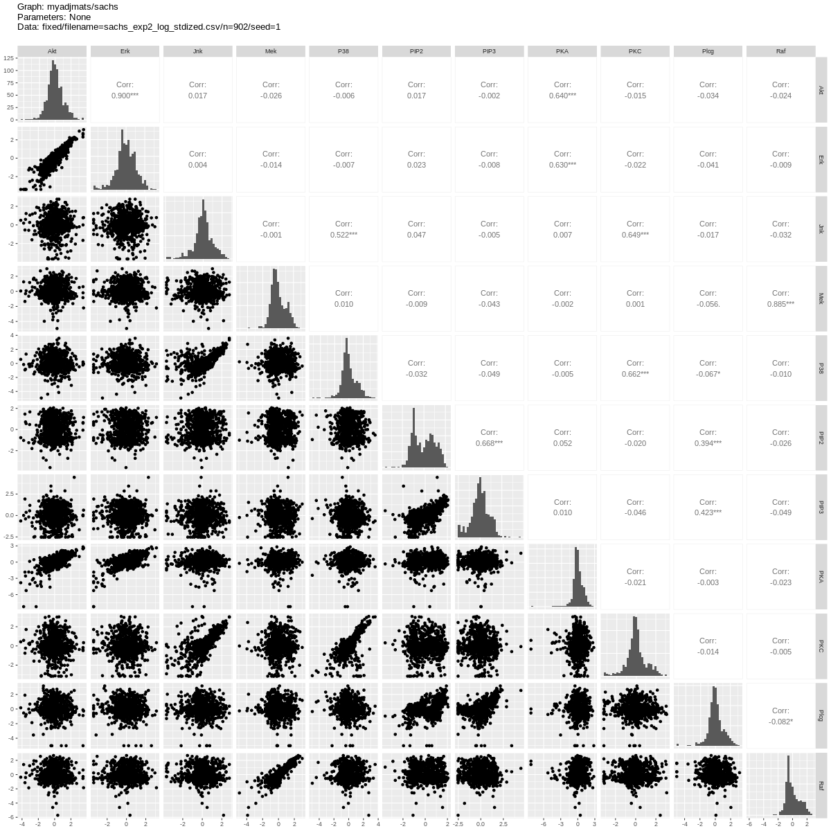
Figure 4: Scatter plots of the logged and standardized data from the second experiment in Sachs et al. (2005) by the ggally_ggpairs module.

Listing 5 shows the object in the data section of the config file defining the data setup. This setup falls into data Scenario II of Table 4 since the graph_id is set to the filename of the graph. For Scenario I, when the underlying graph is unknown, graph_id would be set to null. The full JSON specification for this study is found in paper_sachs.json.

⬇

\par{

"graph_id": "sachs.csv",

"parameters_id": null,

"data_id": "2005_sachs_2_cd3cd28icam2_log_std.csv",

"seed_range": null

}

\par

Figure 5: Scenario II data object for the transformed second dataset from Sachs et al. (2005).

Figure 6(a) shows SHD based on the CPDAG and $F_{1}$ score based on the undirected skeleton from 11 algorithms with different parametrisations, produced by the benchmarks module. From this figure we can directly conclude that all algorithms have a parametrisation that gives the minimal SHD of 9 and maximal $F_{1}$ score of 0.67. Figure 7(a) and Figure 7(b) show the adjacency matrix and DAG plots, respectively, produced by the graph_plots module of the DAG estimated by the bnlearn_tabu module. Figure 8 shows the pattern graph of both the true (Figure 8(a)) and a DAG (Figure 8(b)) estimated by the bnlearn_tabu module, where the black edges are correct in both subfigures. The missing and incorrect edges are coloured in blue and red respectively in Figure 8(b).

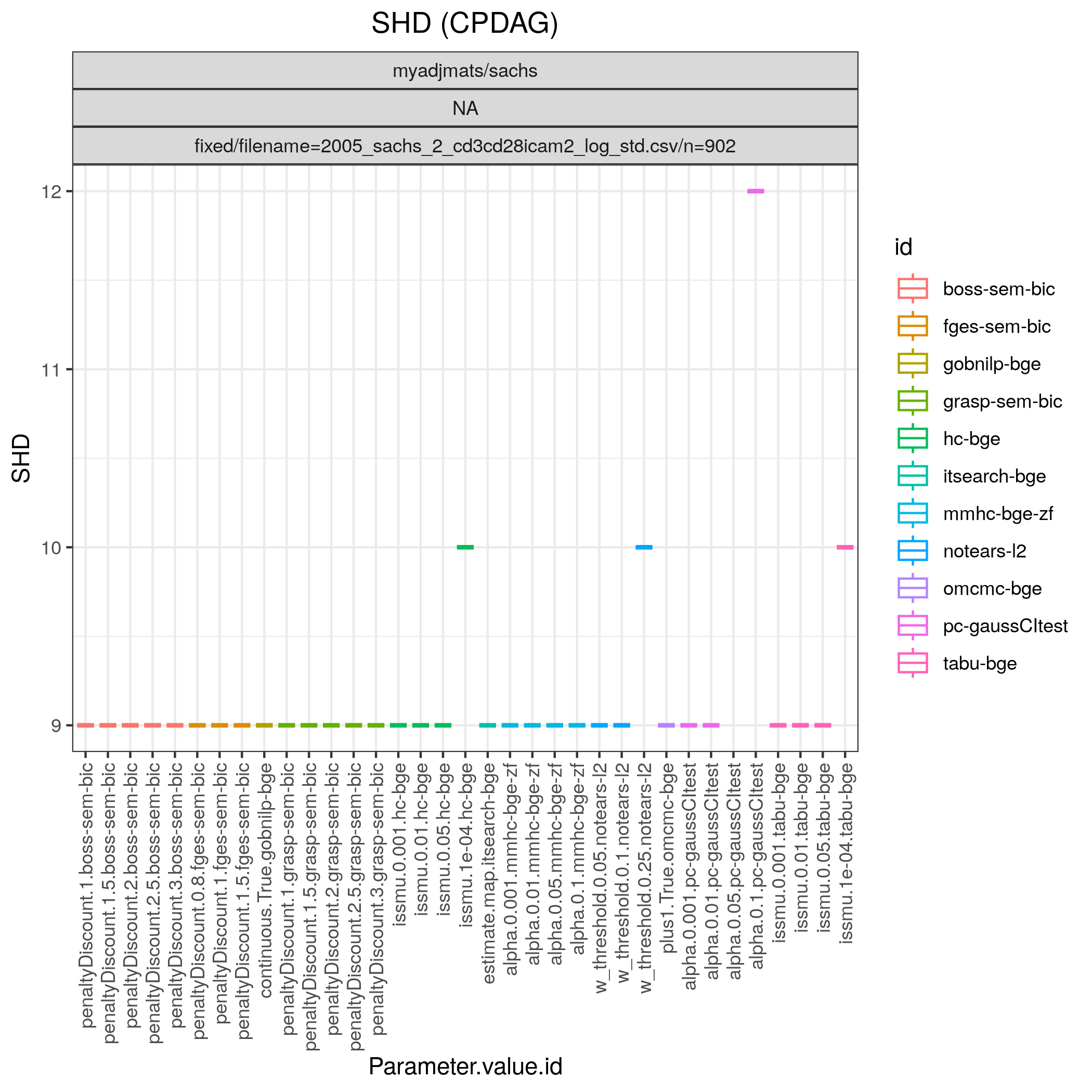
(a)

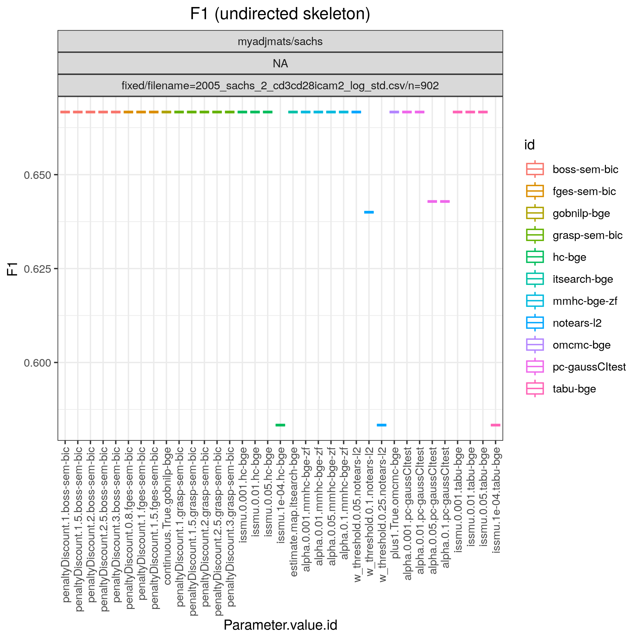
(b)

Figure 6: SHD (6(a)) based on the CPDAG and $F_{1}$ score (6(b)) based on the skeleton produced by the benchmarks module.

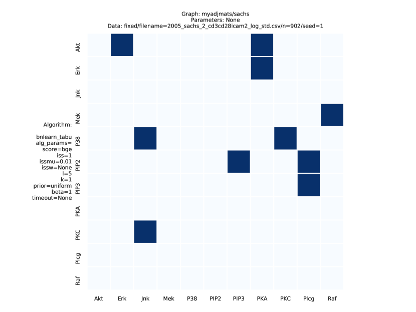
(a)

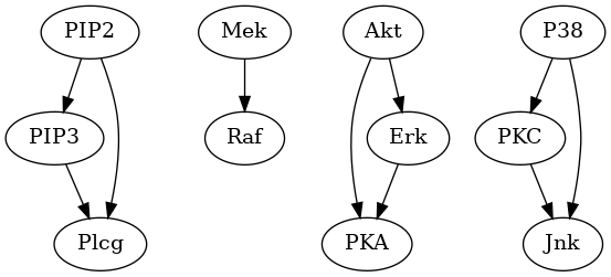
(b)

Figure 7: Adjacency matrix (7(a)) and graph (7(b)) plots produced by the graph_plots module for the Tabu estimate.

(a)

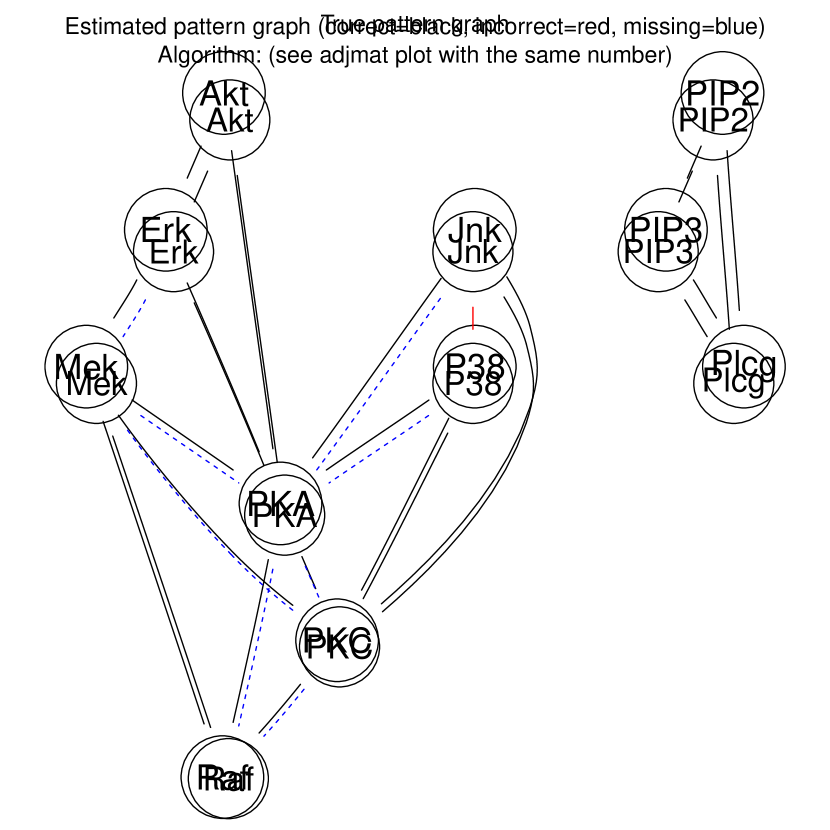
(b)

Figure 8: True pattern graph (8(a)) along with a comparison to the estimated pattern graph (8(b)), using the graph_plots module for the Tabu estimate shown in Figure 7), with parameters as in Figure 7(a)).

5.3 Linear Gaussian SEM with random weights and random DAGs (small scale study)

In the present study we consider a broader simulation over 11 algorithms in a similar Gaussian data setting as in Section 5.1, with the additional difference that the number of nodes is reduced to 20 and the number of seeds is increased to 20. This study took about 40 minutes to finish on a MacBook Pro 2016 with 3.1 GHz Dual-Core Intel Core i5. The full JSON specification for this study is found in paper_er_sem_small.json.

Figure 9(a) shows the $TP/P$ and $FP/P$ based on pattern graphs and Figure 9(b) shows the computational times. We can directly observe that BOSS (boss-sem-bic), GRaSP (grasp-sem-bic), and the order MCMC (omcmc-bge) have very good performance, though they tend to also have longer computational time. Apart from this, the results of Figure 9(a) may be partitioned into two regions, FGES (fges-sem-bic), HC (hc_sem-bic), and Tabu (tabu-bge) having higher values for both $TP/P$ and $FP/P$ and the rest having lower values for both $TP/P$ and $FP/P$.

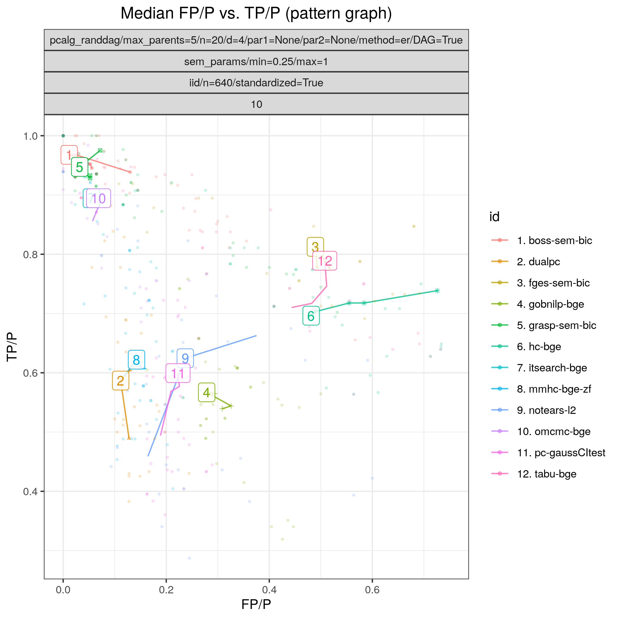
(a)

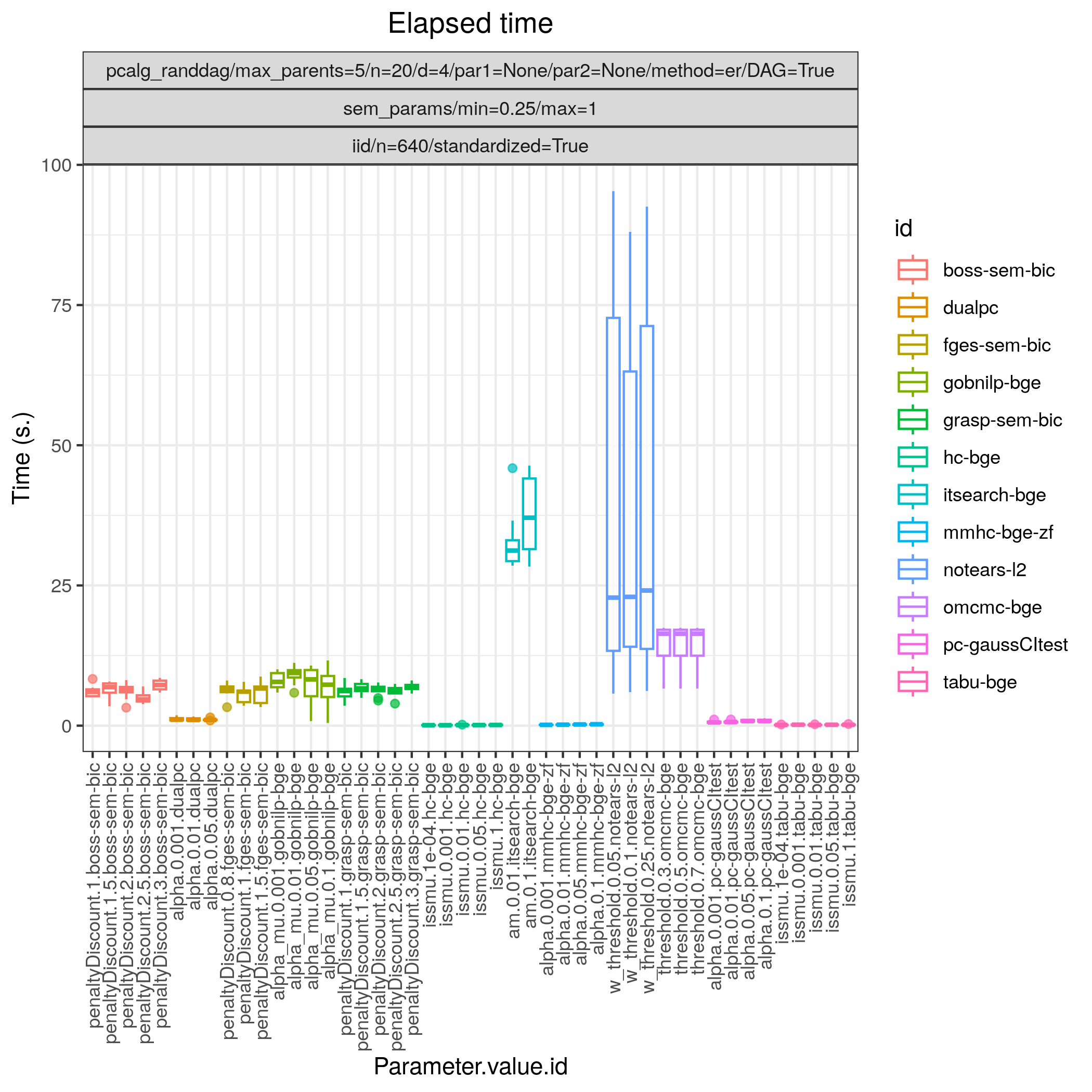
(b)

Figure 9: ROC type curves (9(a)) and timing (9(b)) from the benchmarks module (see caption of Figure 3) evaluated on 20 datasets from a small scale Linear Gaussian SEM with random weights and random DAG.

5.4 Binary valued Bayesian network with random parameters and random DAG

In this example, we study a binary-valued Bayesian network, where both the graph $G$ and the parameters $\Theta$ are regarded as random variables. More specifically, we consider 100 models $\{(G_{i},\Theta_{i})\}_{i=1}^{100}$, where each $G_{i}$ is sampled according to the Erdős-Rényi random DAG model using the pcalg_randdag  module (Appendix B.1), where the number of nodes is $p=80$, the average number of neighbours (parents) per node is 4 (2) and the maximal number of parents per node is 5. The parameters $\Theta_{i}$ are sampled using the bin_bn  module (Appendix B.2) and restricting the conditional probabilities within the range $[0.1,0.9]$. From each model, we draw one dataset $\mathbf{Y}_{i},$ of size $n=320$ using the iid  module. The full JSON specification for this study is found in paper_er_bin.json.

Figure 10(a) shows the ROC type curves for the algorithms considered for the data generated as described above. The algorithms standing out in terms of low SHD in combination with low best median $FP/P$ $(<0.12)$ and higher best median $TP/P$ $(>0.5)$ are BOSS (boss-bdeu), GRaSP (grasp-bdeu), FGES (fges-bdeu), followed by iterative order MCMC (omcmc-bde).

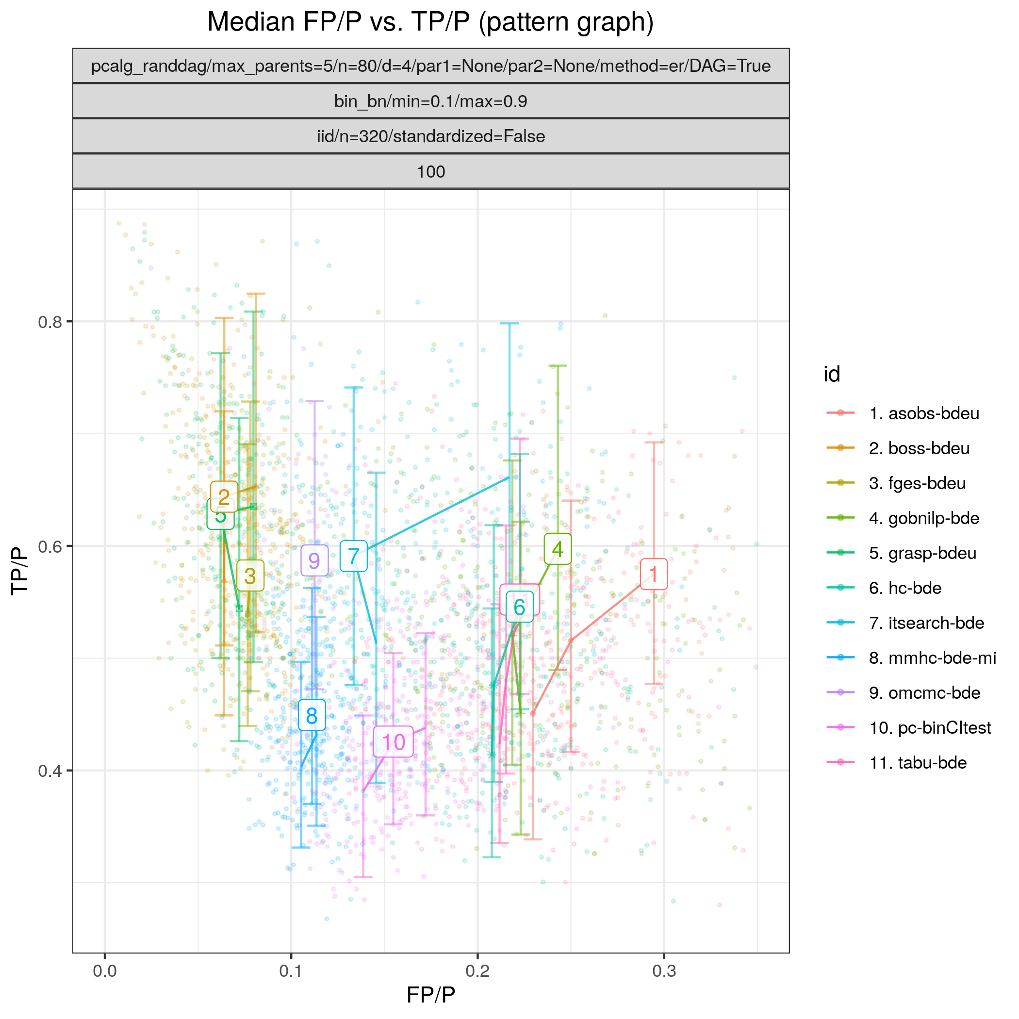
(a) Binary valued Bayesian network with random parameters and random DAG.

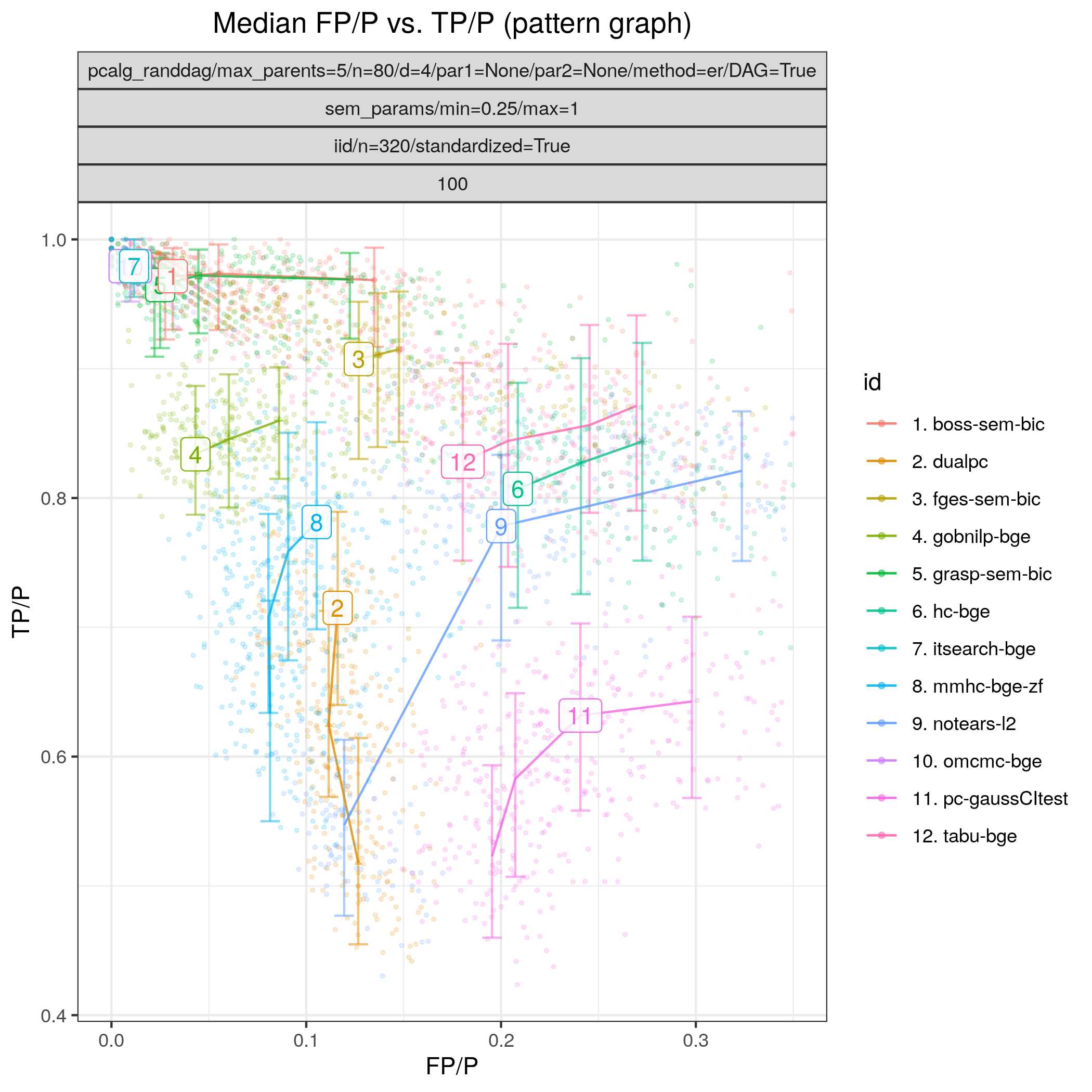
(b) Linear Gaussian SEM with random weights and random DAG.

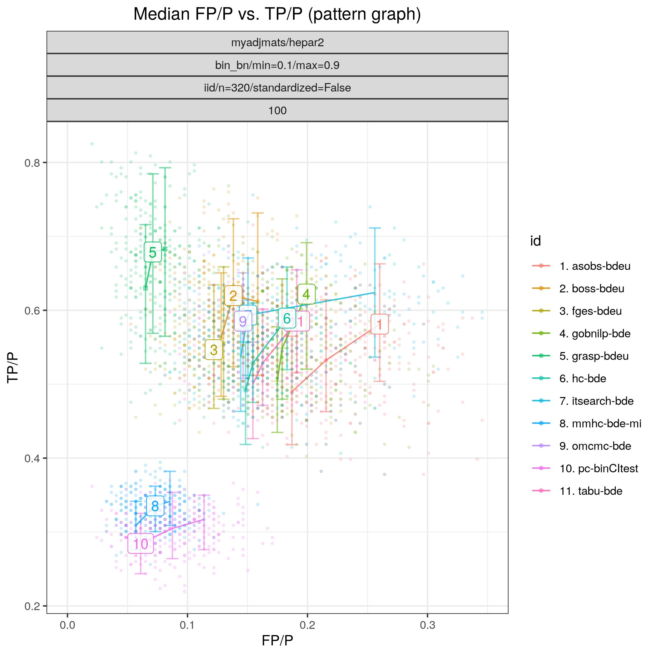
(c) Binary valued Bayesian network with random parameters and (fixed) HEPAR II DAG.

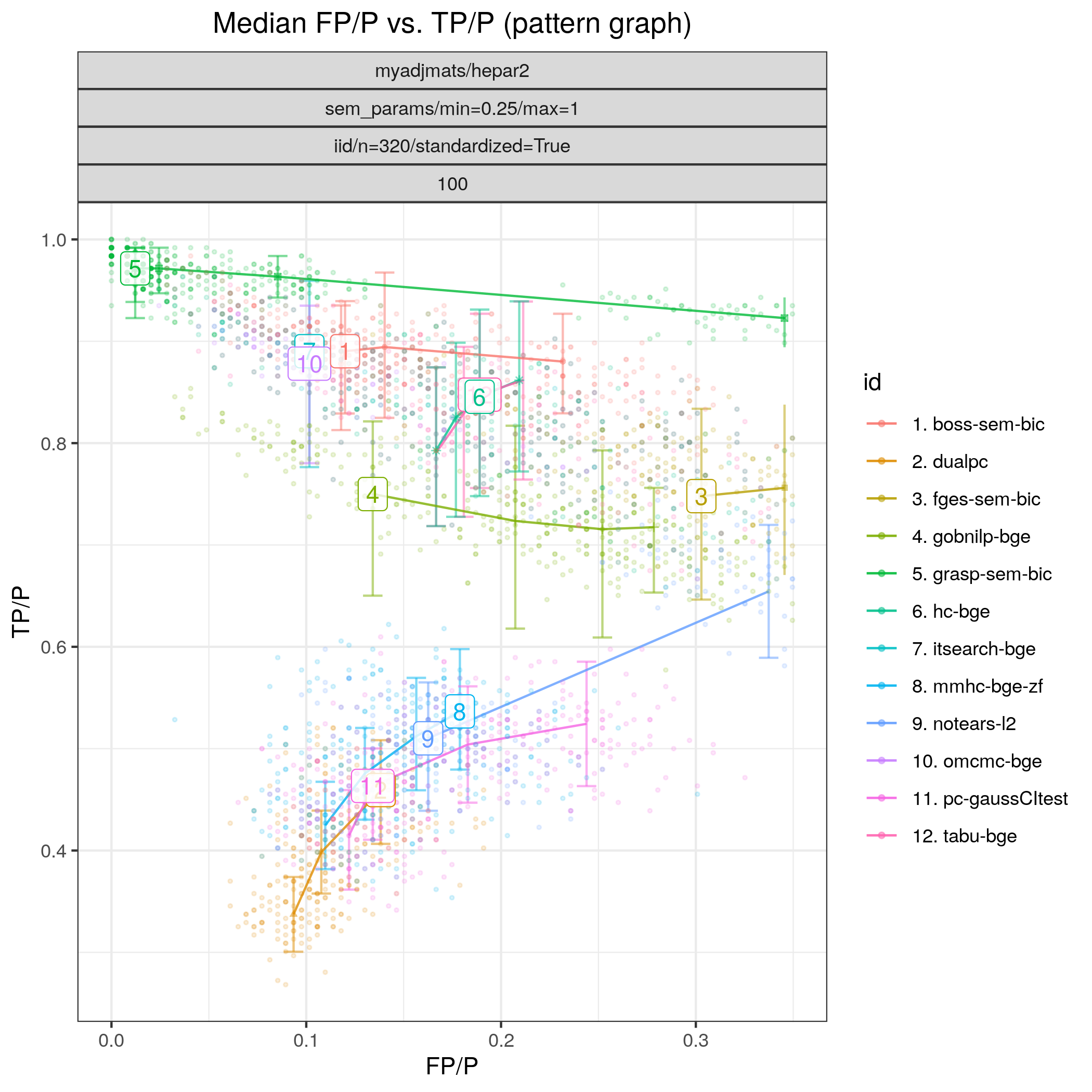
(d) Linear Gaussian SEM with random weights and (fixed) HEPAR II DAG.

Figure 10: ROC type curves (see the caption of Figure 3 for further details) showing the $FP/P$ and $TP/P$ evaluated on 100 datasets from 4 different Bayesian network models.

5.5 Linear Gaussian SEM with random weights and random DAG

In this example, we again study Gaussian random Bayesian networks, of size $p=80$ and with 100 repetitions $\{(G_{i},\Theta_{i})\}_{i=1}^{100}$. We use the same module configurations as in Sections 5.1 and 5.3 and draw one standardised dataset $\mathbf{Y}_{i}$, of size $n=320$ from each of the models using the iid  module. The full JSON specification for this study is found in paper_er_sem.json.

Figure 10(b) shows ROC type results for all the algorithms considered for the data generated as described above. The constraint-based methods PC (pc-gaussCItest) and dual PC (dualpc) have comparable and lower best median $TP/P$ ($<0.7$) than the remaining algorithms. In terms of achieving high $TP/P$ ($>0.9$) iterative order MCMC (omcmc-bge) and iterative search MCMC (itsearch-bge) followed by BOSS (boss-sem-bic) and GRaSP (grasp-sem-bic) stand out with near perfect performance, i.e., SHD $\approx 0$. Among the other algorithms GOBNILP (gobnilp-bge) performs next best with $TP/P$ $\approx 0.85$ and $FP/P$ $\approx 0.08$ followed by FGES (fges-sem-bic).

5.6 Bayesian network with random parameters and fixed DAG

In this example, we study a random binary Bayesian network where the graph $G$ is fixed and the associated parameters $\Theta$ are regarded as random. More specifically, we consider 100 models $\{(G,\Theta_{i})\}_{i=1}^{100}$, where the graph structure $G$ is that of the well known Bayesian network HEPAR II (hepar2.csv), first introduced in Onisko (2003). This graph has 70 nodes and 123 edges and has become one of the standard benchmarks for evaluating the performance of structure learning algorithms. The maximum number of parents per node is 6 and we sample the parameters $\Theta_{i}$ using the bin_bn  module (Appendix B.2), in the same manner as described in Section 5.4. From each model we draw, as before, one dataset $\mathbf{Y}_{i}$ of sample size $n=320$, using the iid  module. The full JSON specification for this study is found in paper_hepar2_bin.json.

Figure 10(c) shows the ROC type curves for this scenario. The algorithms appear to divide between two groups with respect to their performance in terms of $TP/P$. Constraint-based methods including PC (pc-binCItest), and MMHC (mmhc-bde-mi) appear to cluster in the lower scoring region ($TP/P$ $<0.5$). Score-based methods on the other hand seem to concentrate in the higher-scoring region ($TP/P$ $>0.5$). The best performing algorithm is clearly GRaSP (grasp-bdeu) followed by a group of algorithms including FGES (fges-bdeu), BOSS (boss-bdeu), iterative order MCMC (omcmc-bde), and iterative search MCMC (itsearch-bde), all with $FP/P$ $\approx 0.15$.

5.7 Linear Gaussian SEM with random weights and fixed DAG

In this example we draw again 100 models $\{(G,\Theta_{i})\}_{i=1}^{100}$, where $G$ corresponds to the HEPAR II network (hepar2.csv), and $\Theta_{i}$ are the parameters of a linear Gaussian SEM sampled using the sem_params  module (Appendix B.2) with the same settings as in Section 5.5. From each of the models $(G,\Theta_{i})$, we draw one standardised dataset $\mathbf{Y}_{i}$ of size $n=320$ (iid). The full JSON specification for this study is found in paper_hepar2_sem.json.

The ROC-type curves of Figure 10(d) highlight that GRaSP (grasp-sem-bic) again separates itself from the rest of the best algorithms with the more favourable performance. Next follows order MCMC (omcmc-bge), iterative search MCMC (itsearch-bge), and BOSS (boss-sem-bic). In terms of best median $TP/P$ ($>0.8$) only HC (hc-bge) and Tabu (tabu-bge) display similar performances, while performing considerably worse with respect to median $FP/P$ ($\approx 0.1$ vs $\approx 0.17$).

6 Installation and usage

6.1 Requirements

can run either natively on Linux systems, or through Docker, which enables it to run also on macOS and Windows. In either alternative, the first step is to clone the git repository from https://github.com/felixleopoldo/benchpress and set it to the working directory:

    $ git clone https://github.com/felixleopoldo/benchpress.git
    $ cd benchpress

6.1.1 Native (Linux)

Running the workflow natively requires $(\geq 7.30.1)$ and Apptainer (Kurtzer et al., 2017) to be installed on a Linux system. See the documentation of and Apptainer for specific installation instructions. If is installed with conda (Anaconda, 2016, as suggested in ’s documentation) in an environment named e.g. snakemake, it should be activated by:

    $ conda activate snakemake

6.1.2 Docker (Linux/macOS/Windows)

For this alternative, the only requirement is Docker, which can be installed following the instructions on their official website. The commands are then executed from an interactive shell of the Docker image bpimages/snakemake:v7.32.3, where both and Apptainer are installed. The working directory (the benchpress directory) is a shared volume and is mounted in the /mnt folder. The command is:

$ docker run -it -w /mnt --privileged -v $(pwd):/mnt bpimages/snakemake:v7.32.3

Windows users should substitute $(pwd) for the absolute path to the benchpresss folder.

6.2 Usage

Configuration files are executed through standard commands, with the use-singularity flag on. For example, the following command will use all the available cores to run the config file config/config.json

    $ snakemake --cores all --use-singularity --configfile config/config.json

For alternative use cases, e.g. execution in the cloud or on a grid, we refer to the documentation of .

7 New modules

One of the main strengths of is that the modular design provides a flexible framework to integrate new modules into any of the module sections. Next, we demonstrate how to add a new module, update the documentation, and push it upstream.

7.1 Adding new modules

In this section, we show an example of how to add a new structure learning module. Adding parameterization and data modules is done similarly. To get started, copy the template module new_alg to a new module that we name mymod. To do this (macOS/Linux) type the following command from the benchpress folder:

    $ cp -r resources/module_templates/new_alg \
    workflow/rules/structure_learning_algorithms/mymod

This will create the new module mymod (in workflow/rules/structure_learning_algorithms/mymod) which is ready to be used alongside the existing ones.

The module contains files that are needed for the module’s functionality and documentation. It is pre-configured in rule.smk (Listing 11, Line 13) to run the template script.R (Listing 12), which implements an algorithm that merely samples a random binary symmetric matrix. The snakemake variable, used in script.R, is an object that provides access to the input (Listing 11, Line 4) and output (Listing 11, Line 6) fields of rule.smk (Listing 12, Lines 18, 20, and 21) and to the module’s JSON object keys through the wildcards list (Listing 11, Lines 7, 10). Note that, the keys of the wildcards list are directly inherited from the keys of the JSON object used in the config file, see Listing 13 for an example. The wildcards list also contains the random seed number (Listing 12, Line 7) stemming from the seed_range specified in the data_setup section of the config file.

In the simplest case when adapting the module to your algorithm, you essentially only have to alter the rows between Lines 9-14 in Listing 12 and the keys of the JSON object. The module will by default run in a container based on the Docker image bpimages/sandbox:1.0, where both R and Python are installed. This may be changed to any suitable image that supports, e.g. a Docker image at Docker Hub. To force local execution, which might be desirable when developing a new algorithm, the container field of rule.smk (Listing 11, Line 11) should be set to None.

Note that the actual algorithm is embedded in the function called myalg, which is passed to the function add_timeout. This enables a timeout functionality, which writes an empty file if the algorithm has not finished before timeout seconds, specified in the config file. However, if the algorithm can produce a graph estimate after a pre-specified amount of time, that graph should preferably be written.

The module template also contains a Python script, script.py, which could directly replace script.R in rule.smk (Listing 11, Line 13). For other languages and further details about customising rules, we refer to ’s official documentation.

⬇

rule:

name:

module_name

input:

data = alg_input_data()

output:

adjmat = alg_output_adjmat_path(module_name),

time = alg_output_time_path(module_name),

ntests = alg_output_ntests_path(module_name)

container:

"docker://bpimages/sandbox:1.0"

script:

"script.R"

Figure 11: rule file rule.smk of the new_alg template.

⬇

source("workflow/scripts/utils/helpers.R")

\parmyalg <- function() {

data <- read.csv(snakemake@input[["data"]], check.names = FALSE)

start <- proc.time()[1]

p <- ncol(data)

set.seed(as.integer(snakemake@wildcards[["seed"]]))

\par# Naive algorithm start

cutoff <- as.numeric(snakemake@wildcards[["cutoff"]])

adjmat <- matrix(runif(p * p), nrow = p, ncol = p) > cutoff

adjmat <- 1 * (adjmat | t(adjmat))

diag(adjmat) <- 0

# Naive algorithm end

\partotaltime <- proc.time()[1] - start

colnames(adjmat) <- names(data) # Get the labels from the data

write.csv(adjmat, file = snakemake@output[["adjmat"]],

row.names = FALSE, quote = FALSE)

write(totaltime, file = snakemake@output[["time"]])

write("None", file = snakemake@output[["ntests"]])

}

\paradd_timeout(myalg)

Figure 12: The R-script script.R for the new_alg template module.

⬇

{

"id": "testing_myalg",

"cutoff": 0.8,

"timeout": null

}

Figure 13: Example JSON object for the new_alg template module.

7.2 Documentation

The documentation for a module can easily be generated based on information provided by the files in the modules folder. The files and their purpose are described next. The file schema.json is a JSON schema for restricting the fields of a module’s JSON objects, forcing the user to provide valid input parameters. It also allows the developer to provide a description of each of the input parameters. The file info.json should be filled with meta-information about the module, in terms of e.g. version number, links to the documentation, and the type of graph the module supports. bibtex.bib is a BibTeX file where the references, relevant to the module can be added. docs.rst is a documentation file in reStructuredText format that should contain an overview of the module and relevant information.

To generate an HTML version of the documentation using sphinx, the following commands should be executed from the benchpress directory (macOS/Linux):

    $ pip install -r docs/source/requirements.txt    $ cd docs    $ chmod +x render_docs.sh    $ ./render_docs.sh    $ make htmlThe documentation can be seen by opening docs/build/html/index.html with a web browser.

7.3 Contributing

The instructions above show how to integrate a new module into . To add a module to the official repository, the module should run on a Docker or Apptainer image available at e.g. Docker Hub. Publishing modules (or any contributions) to is done by creating a so-called fork of the ’s GitHub repository (https://github.com/felixleopoldo/benchpress) and creating a so-called pull request.

7.4 Reproducibility

All the pieces of information used to build the benchmarks in are saved as files that are easily accessible. For all the simulations, uses fixed random seeds to ensure that the code will produce the same results again. Using Docker and Apptainer makes it easy to reproduce results on essentially any modern computer. When a new module is published, we encourage the developer to attach one or more config files that highlight important properties of the modules along with a few example output figures in docs.rst.

8 Conclusions

provides a novel workflow for scalable and reproducible execution and benchmarking of structure learning algorithms. ’s support for running containerized software through Apptainer together with the simple data and graph representation enables to compare algorithms implemented in different programming languages and run them without requiring unnecessary system privileges or installation of individual module dependencies. is the first software of its kind for structure learning in many aspects, including scalability and reproducibility, and perhaps most importantly from the fact that it can directly incorporate existing software. This can potentially save researchers a large amount of unnecessary work and provide benchmarks that would never be implemented otherwise. Likewise, it could facilitate necessary benchmarks for new algorithms, and the sharing of the results in a standardised format. In its current version already implements 54 of the state-of-the-art learning algorithms, as well as several modules for generating data models and evaluating performance. As is built in a completely modular form allows for seamless scaling of computations over multiple cores, grids or servers without any extra additional effort. In addition, it is straightforward to integrate new modules into the workflow. Even though the project focusses so far on structure learning for graphical models, we also see the potential in extending to evaluate more general estimation procedures, also for other statistical models.

Appendix A Graph metrics and data formats

A.1 Metrics

This section describes metrics for comparing graphs. We let $G=(V,E)$ and $G^{\prime}=(V^{\prime},E^{\prime})$ denote the true and the estimated graph, respectively.

A.1.1 Structural Hamming distance

The structural Hamming distance (SHD) is one of the most commonly used metrics to compare graphs. It describes the number of changes, in terms of adding, removing or reversing edges or their directions, needed to transform $E$ into $E^{\prime}$.

A.1.2 True and false positive rates for mixed graphs

The following metric quantifies the difference between two mixed graphs, which may have a combination of directed and undirected edges. We let $TP$ and $FP$ be the true and also positive edge rates, but for directed edges, we include errors in their direction (wrong direction or directed where it should be undirected, or vice versa) as half a false positive ($FP$) and half a false negative ($FN$).

We assign to every edge $e\in E^{\prime}$ the true positive score $TP(e)=1$ if $e$ is contained in $E$ with the same orientation ($e$ being undirected in both $E$ and $E^{\prime}$ or $e$ having the same direction in both $E$ and $E^{\prime}$), $TP(e)=1/2$ if $e$ is contained in $E$ with a different orientation (or undirected when should be directed, or vice versa), otherwise $TP(e)=0$.

The false positive score $FP(e)$ is defined analogously for every edge $e\in E^{\prime}$. $FP(e)=1$ if no orientation of $e$ is contained in $E$ and $FP(e)=1/2$ if $e$ is contained in $E$ with a different orientation (or undirected when should be directed, or vice versa), otherwise $FP(e)=0$.

The total true and false positive edges ($TP$ and $FP$) are obtained as the sum of the individual edge scores, i.e.

$$TP:=\sum_{e\in E^{\prime}}TP(e),\quad FP:=\sum_{e\in E^{\prime}}FP(e)$$

and the false negative edges ($FN$) are defined as

$$FN:=P-TP,$$

where $P:=|E|$ denotes the total number of edges in $G$. Note that $TP$, $FP$, and $FN$ reduce to the ordinary true and false positives and false negatives, respectively, when all edges are undirected in both $G$ and $G^{\prime}$.

We often consider the scaled true and false positive rates $FP/P$ and $TP/P$, since the SHD, also for mixed graphs, can easily be determined in a ROC-type figure as the scaled Manhattan distance between the points (0,1) and $(TP/P,FP/P)$, i.e.

$$SHD/P=1-TP/P+FP/P.$$

A.1.3 $F$ score

The precision ($PR$) and recall ($RE$) metrics are defined as

$$PR:=\frac{TP}{TP+FP},\quad RE:=\frac{TP}{TP+FN}.$$

For any $\beta\geq 0$ the $F_{\beta}$ score is defined as

$$F_{\beta}:=(1+\beta^{2})\frac{PR\cdot RE}{\beta^{2}PR+RE}.$$

uses $\beta=1$ as default which simplifies to

$$F_{1}=\frac{PR\cdot RE}{PR+RE}=\frac{2TP}{2TP+FP+FN}.$$

A.2 Data formats

Throughout this section for simplicity we consider a four dimensional graphical model where the nodes are labeled as a,b,c and d.

A.2.1 Data set

Observations should be stored as row vectors in a matrix, where the columns are separated by commas. The first row should contain the labels of the variables and if the data is categorical, the second row should contain the cardinality (number of levels) of each variable.

Below is a formatting example of two samples of a categorical distribution where the cardinalities are 2,3,2, and 2.

    a,b,c,d
    2,3,2,2
    1,2,0,1
    0,1,1,1

An example showing of two samples from continuous distribution is shown below.

    a,b,c,d
    0.2,2.3,5.3,0.5
    3.2,1.5,2.5,1.2

A.2.2 Adjacency matrix

A graph $G=(E,V)$ is represented by its adjacency matrix $M$, where $M_{ij}=1$ if $(i,j)\in E$ and $M_{ij}=0$ if $(i,j)\notin E$. An undirected graph is represented by a symmetric matrix.

Below is an example undirected graph $G=(V,E)$, where $E=\{(a,b),(a,c),(c,d)\}$ are interpreted as un-ordered pairs (un-directed edges).

    a,b,c,d
    0,1,1,0
    1,0,0,0
    1,0,0,1
    0,0,1,0

If $G$ is directed the adjacency matrix is asymmetric as below.

    a,b,c,d
    0,1,1,0
    0,0,0,0
    0,0,0,1
    0,0,0,0

A.2.3 MCMC trajectory

When the output of the algorithm is a Markov chain of graphs, we store the output in a compact form by tracking only the changes when moves are accepted, along with the corresponding time index and the score of the resulting graph after acceptance (not the score difference).

Additionally, in the first two rows the labels of the variables, which should be read from the data matrix, are recorded. Specifically, the first row (index -2) contains edges from the first variable to each of the rest in the added column, where a dash (-) symbolises an undirected edge, and a right arrow (->) a directed edge. The score column is set to 0 and removed is set to []. The second row (index -1) has the same edges in the removed column, while the score column is set to 0 and added is set to []. The third row (index 0) contains all the vertices in the starting graph along with its score in the score column and [] in the removed column.

Below is an example of a trajectory of undirected graphs $G_{0},G_{1},\dots,G_{89}$, where $E_{i}=\{(b,c),(a,d)\}$ for $i=0,\dots,33$, $E_{i}=\{(a,d)\}$ for $i=34,\dots,88$ and $E_{i}=\{(c,d),(a,d)\}$ for $i=89$.

    index,score,added,removed
    -2,0.0,[a-b;a-c;a-d],[]
    -1,0.0,[],[a-b;a-c;a-d]
    0,-2325.52,[b-c;a-d],[]
    34,-2311.94,[],[b-c]
    89,-2310.81,[c-d],[]

Appendix B Benchpress modules

B.1 Graph modules

Random graph (pcalg_randdag)
The pcalg_randdag  module samples random undirected graphs and DAGs using the randDAG function from the pcalg package (Kalisch et al., 2012), with the extra option of restricting the maximal number of parents per node.

Fixed graph (fixed_graph)
A fixed graph is represented as an adjacency matrix and should be formatted as specified in Appendix A. The file should be stored with the .csv extension in the directory resources/adjmat/myadjmats/.

B.2 Parameters modules

Random binary Bayesian network (bin_bn)
This module samples the conditional probability tables of a binary Bayesian network (only binary variables). For each variable $Y_{i}$ and parent configuration $pa(y_{i})$

$$pr(Y_{i}=0|pa(y_{i}))\sim\mathrm{Unif}([a,b]),$$

where $(a,b)\in[0,1]^{2},a<b$ and $\mathrm{Unif}(c)$ denotes the uniform distribution on the range $c$.

Random linear Gaussian Bayesian network (sem_params)
This module samples the weight matrix $W$ of a Gaussian linear structural equation model (SEM) of the form

$$Y_{i}=\sum_{j:Y_{j}\in pa(Y_{i})}W_{ij}Y_{j}+Z_{i},$$ (1)

where $Z_{i}\sim\mathcal{N}(\mu,\sigma^{2})$ and elements of $W$ are distributed as

$$W_{ij}\sim\begin{cases}\mathrm{Unif}([a,b])\mathrm{Unif}(\{-1,1\})&\text{ if }(i,j)\in E\\ 0&\text{ otherwise.}\end{cases}$$ (2)

Fixed parameters (fixed_params)
Two types of fixed parameters are currently supported and described below.

• bn.fit object: A Bayesian network object in the R-package bnlearn (Scutari, 2010) is an instance of the bn.fit class and contains both the DAG and corresponding parameters. Motivated by the modular design of , a bn.fit object may be used to specify only the parameters of a Bayesian network, by storing it in .rds format in resources/parameters/myparams/bn.fit_networks/. The adjacency matrix of the DAG should be stored in the folder for fixed_graphs and graph_id should be set to the filename.

• SEM parameters matrix: A matrix defining the weights $W$ in a SEM as defined in (1) can be stored in resources/parameters/myparams/sem_params/ with the .csv extension, formatted as the adjacency matrix specified in Appendix A.

Gaussian graph intra-class model (trilearn_intraclass)
This module specifies the covariance matrix $\Sigma$ of a zero-mean Gaussian graphical model by the solution of the following matrix completion problem

$$\Sigma_{ij} =\begin{cases}\sigma^{2},&\text{ if }i=j\\ \rho\sigma^{2},&\text{ if }(i,j)\in E\end{cases}$$

$$(\Sigma^{-1})_{ij} =0\quad\quad\quad\text{ if }(i,j)\notin E,$$

where $\sigma^{2}>0$ and $\rho\in[0,1]$ denote the variance and correlation coefficient, respectively.

Hyper Dirichlet (trilearn_hyper-dir)
This module samples the parameters of a categorical decomposable model from the hyper Dirichlet distribution (Dawid and Lauritzen, 1993), with a specified concentration parameter and number of levels per variable.

Inverse G-Wishart (bdgraph_rgwish)
This modules samples the precision matrix of a Gaussian graphical model from the G-Wishart distribution (Dawid and Lauritzen, 1993; Atay-Kayis and Massam, 2005; Lenkoski, 2013) using the rgwish function from the BDgraph package (Mohammadi and Wit, 2019). The clique-wise scale matrices are fixed to the identity matrix while the degrees of freedom and a threshold value for the convergence of the sampling algorithm are specified by the user.

B.3 Data modules

Fixed data sets (fixed_data)
The are two ways of providing fixed data sets. The first option is to place data files directly in the directory resources/data/mydatasets/ with the .csv extension, formatted according to Appendix A. The second option is to place the files in a sub directory of resources/data/mydatasets/. In the latter case, the data_id field in the benchmarks_setup section should be the name of the directory and all the files in it will be considered for evaluation.

Independent identically distributed (i.i.d.) samples (iid)
An object of the iid  module will draw a specified (n) number of independent samples from a specified model. Continuous data may be standardized by setting standardized to true. See Reisach et al. (2021) for a discussion about standardising data in a structure learning context.

B.4 Structure learning algorithms

This section contains a short summary of the structure learning modules that are used in the simulation study of Section 5.

Algorithm	Graph	Package	Module
ANM	DAG	gCastle	gcastle_anm
ASOBS	DAG	r.blip	rblip_asobs
BDgraph	UG	BDgraph	bdgraph
BOSS	CPDAG	causal-cmd	tetrad_boss
Chordal graph samplers	DG		athomas_jtsamplers
CORL	DAG	gCastle	gcastle_corl
Corrmat thresh	UG	Benchpress	corr_thresh
Direct LINGAM	DAG	gCastle	gcastle_direct_lingam
Dual PC	CPDAG	dualPC	dualpc
FAS	DAG	causal-cmd	tetrad_fas
FASK	DAG	causal-cmd	tetrad_fask
Fast IAMB	DAG	bnlearn	bnlearn_fastiamb
FGES	CPDAG	causal-cmd	tetrad_fges
FOFC	DAG	causal-cmd	tetrad_fofc
FTFC	DAG	causal-cmd	tetrad_ftfc
GAE	DAG	gCastle	gcastle_gae
GIES	CPDAG	pcalg	pcalg_gies
GOBNILP	DAG	GOBNILP	gobnilp
GOLEM	DAG	gCastle	gcastle_golem
GraNDAG	DAG	gCastle	gcastle_grandag
Graphical Lasso	UG	scikit-learn	sklearn_glasso
GRaSP	CPDAG	causal-learn	causallearn_grasp
GRaSP	CPDAG	causal-cmd	tetrad_grasp
Grow-shrink	DAG	bnlearn	bnlearn_gs
GrUES	UG	gues	grues
GSP	DAG	CausalDAG	causaldag_gsp
H2PC	DAG	bnlearn	bnlearn_h2pc
HC	DAG	bnlearn	bnlearn_hc
HPC	DAG	bnlearn	bnlearn_hpc
IAMB	DAG	bnlearn	bnlearn_iamb
IAMB-FDR	DAG	bnlearn	bnlearn_iambfdr
ICALiNGAM	DAG	gCastle	gcastle_ica_lingam
INTER-IAMB	DAG	bnlearn	bnlearn_interiamb
Iterative search	DAG	BiDAG	bidag_itsearch
LINGAM	DAG	causal-cmd	tetrad_lingam
MCSL	DAG	gCastle	gcastle_mcsl
MMHC	DAG	bnlearn	bnlearn_mmhc
MMPC	DAG	bnlearn	bnlearn_mmpc
NO TEARS	DAG	gCastle	gcastle_notears
NO TEARS low rank	DAG	gCastle	gcastle_notears_low_rank
NO TEARS non-linear	DAG	gCastle	gcastle_notears_nonlinear
Order MCMC	DAG	BiDAG	bidag_order_mcmc
Parallel DG	DG	parallelDG	paralleldg
Particle Gibbs	DG	trilearn	trilearn_pgibbs
Partition MCMC	DAG	BiDAG	bidag_partition_mcmc
PC	CPDAG	bnlearn	bnlearn_pcstable
PC	DAG	gCastle	gcastle_pc
PC	CPDAG	pcalg	pcalg_pc
PC-ALL	DAG	causal-cmd	tetrad_pc-all
Precmat thresh	UG	Benchpress	prec_thresh
Psi-leaner	UG	equSA	equsa_psilearner
RL	DAG	gCastle	gcastle_rl
RSMAX2	DAG	bnlearn	bnlearn_rsmax2
S-I HITON-PC	DAG	bnlearn	bnlearn_sihitonpc
Tabu	DAG	bnlearn	bnlearn_tabu

Table 6: Currently available structure learning modules.

Peter and Clark (pcalg_pc)
The Peter and Clark (PC) algorithm (Spirtes and Glymour, 1991), is a constraint based method consisting of two main steps. The first step is called the adjacency search and amounts to finding the undirected skeleton of the DAG through conditional independence tests. The second step consists of estimating a CPDAG from the skeleton and the previous tests.

Dual PC (dualpc)
The dual PC algorithm (Giudice et al., 2023) is an alternative scheme to carry out the conditional independence tests within the PC algorithm for Gaussian data, by leveraging the inverse relationship between covariance and precision matrices. The algorithm exploits block matrix inversions on the covariance and precision matrices to simultaneously perform tests on partial correlations of complementary (or dual) conditioning sets. Simulation studies indicate that the dual PC algorithm outperforms the classic PC algorithm both in terms of run time and in recovering the underlying network structure.

Hill climbing (bnlearn_hc)
Hill climbing (HC) is a score-based algorithm which starts with a DAG with no edges and adds, deletes or reverses edges in a greedy manner until an optimum is reached (Russell and Norvig, 2002; Scutari et al., 2019b).

Tabu (bnlearn_tabu)
Tabu is a less greedy version of the HC algorithm allowing for non-optimal moves that might be beneficial from a global perspective to avoid local maxima (Russell and Norvig, 2002; Scutari et al., 2019b).

Best Order Score Search (tetrad_boss)
Best Order Score Search (BOSS) (Ramsey, 2021; Andrews et al., 2023) is a permutation-based algorithm stemming from the Ordering Search of Teyssier and Koller (2012) and the Sparsest Permutation algorithm (SP) of Raskutti and Uhler (2018) as in the Greedy Sparsest Permutation algorithm GSP of Solus et al. (2021). BOSS gives results as accurate as SP but for much larger and denser graphs. It is more accurate for two reason: (a) It assumes the so-called brute faithfuness assumption, which is weaker than faithfulness, and (b) it uses a different traversal of permutations than the depth-first traversal used by GSP, obtained by taking each variable in turn and moving it to the position in the permutation that optimizes the model score.

Fast greedy equivalent search (tetrad_fges)
Fast greedy equivalent search (FGES) is a score based method based on the the greedy equivalence search (GES) of Meek (1997). This algorithm operates on the space of CPDAG’s (Chickering, 2002). Its complexity is polynomial in the number of nodes. The FGES is asymptotically correct under the assumption that there are no unmeasured confounders (Ogarrio et al., 2016), a condition required for most algorithms with convergence guarantees.

Greedy relaxations of the sparsest permutation algorithm (tetrad_grasp)
This is a method that exploits permutation reasoning to search for directed acyclic causal models, like the Ordering Search of Teyssier and Koller (2012) and GSP of Solus et al. (2021). The algorithm extends these methods by a permutation-based operation called tuck, and develops a class of algorithms, namely Greedy relaxations of the sparsest permutation (GRaSP) (Lam et al., 2022), that are computationally efficient and pointwise consistent under increasingly weaker assumptions than faithfulness.

Order Markov chain Monte Carlo (bidag_order_mcmc)
This technique relies on a Bayesian perspective on structure learning and uses the posterior probability of graphs as a score. To overcome the limitation of simple structure-based MCMC schemes, Friedman and Koller (2003) turned to a score defined as the sum of the posterior scores of all DAG which are consistent with a given topological ordering of the nodes. One can then run a Metropolis-Hasting algorithm to sample from the distribution induced by the order score, and later draw a DAG consistent with the order. This strategy substantially improves convergence with respect to earlier structure MCMC scheme, though it unfortunately produces a biased sample on the space of DAGs. The bias can be removed by operating on the space of ordered partitions instead (Kuipers and Moffa, 2017). The implementation considered in is a hybrid version with the sampling performed on a restricted search space initialised with constraint-based testing and improved with a score-based search (Jack Kuipers and Moffa, 2022).

Max-min hill-climbing (bnlearn_mmhc)
Max-min hill-climbing (MMHC) is a hybrid method which first estimates the skeleton of a DAG using an algorithm called Max-Min Parents and Children and then performs a greedy hill-climbing search to orient the edges with respect to a Bayesian score (Tsamardinos et al., 2006). It is a popular approach used as standard benchmark and also well suited for high-dimensional domains.

Globally optimal Bayesian network learning using integer linear programming (gobnilp)
A score based method using integer linear programming (ILP) for learning an optimal DAG for a Bayesian network with limit on the maximal number of parents for each node (Cussens, 2011). It is a two-stage approach where candidate parent sets for each node are discovered in the first phase and the optimal sets are determined in a second phase.

Acyclic selection ordering-based search (rblip_asobs)
A score-based two-phase algorithm where the first phase aims to identify the possible parent sets, Scanagatta et al. (2015, 2018). The second phase performs an optimisation on a modification of the space of node orders introduced in Teyssier and Koller (2012), allowing edges from nodes of higher to lower order, provided that no cycles are introduced.

Iterative search (bidag_itsearch)
This is a hybrid score-based optimisation technique based on Markov chain Monte Carlo schemes (Suter et al., 2023; Jack Kuipers and Moffa, 2022). The algorithm starts from a skeleton obtained through a fast method (e.g. a constraint based method, or GES). Then it performs score and search on the DAGs belonging to the space defined by the starting skeleton. To correct for edges which may be missed, the search space is iteratively expanded to include one additional parent for each variable from outside the current search space. The score and search phase relies on an MCMC scheme producing a chain of DAGs from their posterior probability given the data.

No tears (gcastle_notears)
This score-based method recasts the combinatorial problem of estimating a DAG into a purely continuous non-convex optimization problem over real matrices with a smooth constraint to ensure acyclicity (Zheng et al., 2018).

B.5 Evaluation modules

Standard benchmarking metrics (benchmarks)
The relative performance of algorithms may differ depending on the evaluation metric, and no single metric is generally preferred. Therefore, to get an overall picture of the performance of an algorithm, the benchmarks module supports different metrics. The benchmarks module provides standard benchmarking metrics in terms of computational time, $F_{1}$, $FN$, $TP$, and $FP$, etc. (see Appendix A.1 for definitions). The results are saved systematically in CSV format, which can be analysed using any program.

In addition to the CSV summaries, also provides visual summarises in terms of e.g., box-plots and receiver operating characteristics (ROC) type curves using the R-package ggplot2 (Wickham et al., 2019) (see e.g. Figure 3(a) and Figure 10). Since the true graphs are needed for evaluations, this module works for data scenarios (II-V).

Pair-wise plots of the data (ggally_ggpairs)
The ggally_ggpairs module produces pair-wise plots of the data using the ggpairs function (Emerson et al., 2013) from the R-package GGally (see Figure 4 for an example).

Plot estimated graphs (graph_plots)
The graph_plots module plots and saves the estimated graphs and adjacency matrices (see Figure 7(a) and 7(b) for examples). If the true graph is available it also compares the true to the estimated graphs using graphviz.compare function from the bnlearn package (see Figure 8 for an example).

Plot true graphs (graph_true_plots)
The graph_true_plots module plots the true underlying graphs and corresponding adjacency matrices.

Statistics for true graphs (graph_true_stats)
The graph_true_stats module computes properties of the true underlying graphs and stored in a CSV file and plotted. See Figure 3(b) for an example plot from this module.

MCMC mean graphs (mcmc_heatmaps)
For Bayesian inference it is customary to use MCMC methods to simulate a Markov chain of graphs $\{G^{l}\}_{l=0}^{\infty}$ having the graph posterior as stationary distribution. Suppose we have a realisation of length $M$ of such chain, then the posterior probability of an edge $e$ is estimated by $\frac{1}{M+1-b}\sum_{l=b}^{M}\mathbf{1}_{e}(e^{l})$, where the first samples up to $b$ are disregarded as a burn-in period.

The mcmc_heatmaps module has a list of objects, where each object has an id field for the algorithm object id and a burn-in field (burn_in) for specifying the burn-in period. The estimated probabilities are plotted in heatmaps using seaborn (Waskom, 2021).

MCMC trajectory plots (mcmc_traj_plots)
The mcmc_traj_plots module plots the value of a given functional for the graphs in the MCMC trajectory. The currently supported functionals are the number of edges for the graphs (size) and the score (score). The mcmc_traj_plots module has a list of objects, where each object has an id field for the algorithm object id, a burn-in field (burn_in) and a field specifying the functional to be considered (functional). Since the trajectories may be very long, the user may choose to thin out the trajectory by only considering every graph at a given interval length specified by the thinning field.

MCMC auto-correlation plots (mcmc_autocorr_plots)
The mcmc_autocorr_plots module plots the auto-correlation of a functional of the graphs in a MCMC trajectory. Similar to the mcmc_traj_plots module, the mcmc_autocorr_plots module has a list of objects, where each object has an id, burn_in, thinning, and a functional field. The maximum number of lags after thinning, is specified by the lags field.

References

- Anaconda (2016) Anaconda (2016). “\pkgAnaconda Software Distribution.”
- Andrews et al. (2023) Andrews B, Ramsey J, Sanchez-Romero R, Camchong J, Kummerfeld E (2023). “Fast Scalable and Accurate Discovery of DAGs Using the Best Order Score Search and Grow-Shrink Trees.” In 37th Conference on Neural Information Processing Systems (NeurIPS 2023).
- Atay-Kayis and Massam (2005) Atay-Kayis A, Massam H (2005). “A Monte Carlo Method for Computing the Marginal Likelihood in Nondecomposable Gaussian Graphical Models.” Biometrika, 92(2), 317–335.
- Carvalho (2006) Carvalho CM (2006). Structure and Sparsity in High-Dimensional Multivariate Analysis. Ph.D. thesis, Duke University.
- Chickering (1995) Chickering DM (1995). “A Transformational Characterization of Equivalent Bayesian Network Structures.” In Proceedings of the Eleventh Conference on Uncertainty in Artificial Intelligence, UAI’95, pp. 87–98. Morgan Kaufmann Publishers Inc., San Francisco, CA, USA.
- Chickering (2002) Chickering DM (2002). “Optimal Structure Identification with Greedy Search.” Journal of machine learning research, 3(11), 507–554.
- Chickering et al. (2004) Chickering DM, Heckerman D, Meek C (2004). “Large-Sample Learning of Bayesian Networks is NP-Hard.” Journal of Machine Learning Research, 5, 1287–1330.
- Constantinou et al. (2020) Constantinou AC, Liu Y, Chobtham K, Guo Z, Kitson NK (2020). “The \pkgBayesys Data and Bayesian Network Repository.” Queen Mary University of London, pp. 2–2.
- Constantinou et al. (2021) Constantinou AC, Liu Y, Chobtham K, Guo Z, Kitson NK (2021). “Large-Scale Empirical Validation of Bayesian Network Structure Learning Algorithms with Noisy Data.” International Journal of Approximate Reasoning, 131, 151–188.
- Cowell et al. (2003) Cowell RG, Dawid P, Lauritzen SL, Spiegelhalter DJ (2003). Probabilistic Networks and Expert Systems: Exact Computational Methods for Bayesian Networks. Information Science and Statistics. Springer-Verlag New York. ISBN 9780387987675.
- Cussens (2011) Cussens J (2011). “Bayesian Network Learning with Cutting Planes.” In Proceedings of the Twenty-Seventh Conference on Uncertainty in Artificial Intelligence, UAI’11, pp. 153–160. AUAI Press, Arlington, Virginia, USA.
- Cussens (2020) Cussens J (2020). “\pkgGOBNILP: Learning Bayesian Network Structure with Integer Programming.” In International Conference on Probabilistic Graphical Models, pp. 605–608. PMLR.
- Dawid and Lauritzen (1993) Dawid AP, Lauritzen SL (1993). “Hyper Markov Laws in the Statistical Analysis of Decomposable Graphical Models.” The Annals of Statistics, 21(3), 1272–1317.
- Diestel (2005) Diestel R (2005). Graph Theory (Graduate texts in mathematics), volume 173. Springer Heidelberg.
- Duarte and Solus (2021) Duarte E, Solus L (2021). “A New Characterization of Discrete Decomposable Models.” arXiv preprint arXiv:2105.05907.
- Edwards (2012) Edwards D (2012). Introduction to Graphical Modelling. Springer-Verlag Science & Business Media.
- Elmasri (2017) Elmasri M (2017). “On Decomposable Random Graphs.” arXiv preprint arXiv:1710.03283.
- Elwert (2013) Elwert F (2013). “Graphical Causal Models.” In Handbook of causal analysis for social research, pp. 245–273. Springer-Verlag.
- Emerson et al. (2013) Emerson JW, Green WA, Schloerke B, Crowley J, Cook D, Hofmann H, Wickham H (2013). “The Generalized Pairs Plot.” Journal of Computational and Graphical Statistics, 22(1), 79–91.
- Friedman et al. (2008) Friedman J, Hastie T, Tibshirani R (2008). “Sparse Inverse Covariance Estimation with the Graphical Lasso.” Biostatistics, 9(3), 432–441.
- Friedman (2004) Friedman N (2004). “Inferring Cellular Networks using Probabilistic Graphical Models.” Science, 303(5659), 799–805.
- Friedman et al. (1997) Friedman N, Goldszmidt M, Heckerman D, Russell S (1997). “Where is the Impact of Bayesian Networks in Learning.” In International Joint Conference on Artificial Intelligence. Citeseer.
- Friedman and Koller (2003) Friedman N, Koller D (2003). “Being Bayesian About Network Structure. A Bayesian Approach to Structure Discovery in Bayesian Networks.” Machine Learning, 50(1), 95–125.
- Friedman et al. (2000) Friedman N, Linial M, Nachman I, Pe’er D (2000). “Using Bayesian Networks to Analyze Expression Data.” Journal of computational biology, 7(3-4), 601–620.
- Geiger and Heckerman (1994) Geiger D, Heckerman D (1994). “Learning Gaussian Networks.” In Proceedings of the Tenth international conference on Uncertainty in artificial intelligence, pp. 235–243. Morgan Kaufmann Publishers Inc.
- Geiger et al. (2002) Geiger D, Heckerman D, et al. (2002). “Parameter Priors for Directed Acyclic Graphical Models and the Characterization of Several Probability Distributions.” The Annals of Statistics, 30(5), 1412–1440.
- Giudice et al. (2023) Giudice E, Kuipers J, Moffa G (2023). “The dual PC algorithm and the role of Gaussianity for structure learning of Bayesian networks.” International Journal of Approximate Reasoning, 161, 108975.
- Giudici and Castelo (2003) Giudici P, Castelo R (2003). “Improving Markov Chain Monte Carlo Model Search for Data Mining.” Machine learning, 50(1), 127–158.
- Giudici and Green (1999) Giudici P, Green PJ (1999). “Decomposable Graphical Gaussian Model Determination.” Biometrika, 86(4), 785–801.
- Glymour and Scheines (1986) Glymour C, Scheines R (1986). “Causal Modeling with the \pkgTETRAD Program.” Synthese, 68(1), 37–63.
- Göbler et al. (2023) Göbler K, Windisch T, Pychynski T, Sonntag S, Roth M, Drton M (2023). “\pkgcausalAssembly: Generating Realistic Production Data for Benchmarking Causal Discovery.” arXiv preprint arXiv:2306.10816.
- Green and Thomas (2013) Green PJ, Thomas A (2013). “Sampling Decomposable Graphs using a Markov Chain on Junction Trees.” Biometrika, 100(1), 91–110.
- Hauser and Bühlmann (2012) Hauser A, Bühlmann P (2012). “Characterization and Greedy Learning of Interventional Markov Equivalence Classes of Directed Acyclic Graphs.” The Journal of Machine Learning Research, 13(1), 2409–2464.
- Hebert-Johnson et al. (2023) Hebert-Johnson U, Lokshtanov D, Vigoda E (2023). “Counting and Sampling Labeled Chordal Graphs in Polynomial Time.” arXiv preprint arXiv:2308.09703.
- Heckerman et al. (1995) Heckerman D, Geiger D, Chickering DM (1995). “Learning Bayesian Networks: The Combination of Knowledge and Statistical Data.” Machine learning, 20(3), 197–243.
- Jack Kuipers and Moffa (2022) Jack Kuipers PS, Moffa G (2022). “Efficient Sampling and Structure Learning of Bayesian Networks.” Journal of Computational and Graphical Statistics, 31(3), 639–650.
- Jennings and Corcoran (2018) Jennings D, Corcoran JN (2018). “A Birth and Death Process for Bayesian Network Structure Inference.” Probability in the Engineering and Informational Sciences, 32(4), 615–625.
- Kalisch et al. (2012) Kalisch M, Mächler M, Colombo D, Maathuis MH, Bühlmann P (2012). “Causal Inference using Graphical Models with the \proglangR Package \pkgpcalg.” Journal of Statistical Software, 47(11), 1–26.
- Kitson et al. (2023) Kitson NK, Constantinou AC, Guo Z, Liu Y, Chobtham K (2023). “A survey of Bayesian Network structure learning.” Artificial Intelligence Review, pp. 1–94.
- Koller and Friedman (2009) Koller D, Friedman N (2009). Probabilistic Graphical Models - Principles and Techniques. MIT Press. ISBN 978-0-262-01319-2.
- Koski and Noble (2012) Koski T, Noble J (2012). “A Review of Bayesian Networks and Structure Learning.” Mathematica Applicanda, 40(1), 51–103.
- Köster and Rahmann (2012) Köster J, Rahmann S (2012). “\pkgSnakemake—A Scalable Bioinformatics Workflow Engine.” Bioinformatics, 28(19), 2520–2522.
- Kuipers and Moffa (2017) Kuipers J, Moffa G (2017). “Partition MCMC for Inference on Acyclic Digraphs.” Journal of the American Statistical Association, 112(517), 282–299.
- Kuipers and Moffa (2022) Kuipers J, Moffa G (2022). “The Interventional Bayesian Gaussian Equivalent Score for Bayesian Causal Inference with Unknown Soft Interventions.” arXiv preprint arXiv:2205.02602.
- Kuipers et al. (2014) Kuipers J, Moffa G, Heckerman D, et al. (2014). “Addendum on the Scoring of Gaussian Directed Acyclic Graphical Models.” The Annals of Statistics, 42(4), 1689–1691.
- Kuipers et al. (2019) Kuipers J, Moffa G, Kuipers E, Freeman D, Bebbington P (2019). “Links Between Psychotic and Neurotic Symptoms in the General Population: An Analysis of Longitudinal British National Survey Data using Directed Acyclic Graphs.” Psychological Medicine, 49(3), 388–395.
- Kuipers et al. (2018) Kuipers J, Thurnherr T, Moffa G, Suter P, Behr J, Goosen R, Christofori G, Beerenwinkel N (2018). “Mutational Interactions Define Novel Cancer Subgroups.” Nature communications, 9(1), 1–10.
- Kurtzer et al. (2017) Kurtzer GM, Sochat V, Bauer MW (2017). “\pkgSingularity: Scientific Containers for Mobility of Compute.” PloS one, 12(5), e0177459.
- Lam et al. (2022) Lam WY, Andrews B, Ramsey J (2022). “Greedy relaxations of the sparsest permutation algorithm.” In Proceedings of the Thirty-Eighth Conference on Uncertainty in Artificial Intelligence, volume 180 of Proceedings of Machine Learning Research, pp. 1052–1062. PMLR.
- Lamprecht et al. (2020) Lamprecht AL, Garcia L, Kuzak M, Martinez C, Arcila R, Martin Del Pico E, Dominguez Del Angel V, van de Sandt S, Ison J, Martinez PA, McQuilton P, Valencia A, Harrow J, Psomopoulos F, Gelpi JL, Chue Hong N, Goble C, Capella-Gutierrez S (2020). “Towards FAIR Principles for Research Software.” 3(1), 37–59.
- Lauritzen (1996) Lauritzen SL (1996). Graphical Models. Oxford University Press. ISBN 0-19-852219-3.
- Lenkoski (2013) Lenkoski A (2013). “A Direct Sampler for G-Wishart Variates.” Stat, 2(1), 119–128.
- Madigan et al. (1995) Madigan D, York J, Allard D (1995). “Bayesian Graphical Models for Discrete Data.” International Statistical Review / Revue Internationale de Statistique, 63(2), 215–232.
- Meek (1997) Meek C (1997). Graphical Models: Selecting Causal and Statistical Models. Ph.D. thesis, PhD thesis, Carnegie Mellon University.
- Meinshausen (2008) Meinshausen N (2008). “A Note on the Lasso for Gaussian Graphical Model Selection.” Statistics and Probability Letters, 78(7), 880 – 884.
- Merkel (2014) Merkel D (2014). “\pkgDocker: Lightweight Linux Containers for Consistent Development and Deployment.” Linux journal, 2014(239), 2.
- Moffa et al. (2017) Moffa G, Catone G, Kuipers J, Kuipers E, Freeman D, Marwaha S, Lennox BR, Broome MR, Bebbington P (2017). “Using Directed Acyclic Graphs in Epidemiological Research in Psychosis: An Analysis of the Role of Bullying in Psychosis.” Schizophrenia Bulletin, 43(6), 1273–1279.
- Mohammadi and Wit (2019) Mohammadi R, Wit EC (2019). “BDgraph: An R Package for Bayesian Structure Learning in Graphical Models.” Journal of Statistical Software, Articles, 89(3), 1–30.
- Montagna et al. (2023) Montagna F, Mastakouri AA, Eulig E, Noceti N, Rosasco L, Janzing D, Aragam B, Locatello F (2023). “Assumption violations in causal discovery and the robustness of score matching.” arXiv preprint arXiv:2310.13387.
- Munafò et al. (2017) Munafò MR, Nosek BA, Bishop DVM, Button KS, Chambers CD, Percie du Sert N, Simonsohn U, Wagenmakers EJ, Ware JJ, Ioannidis JPA (2017). “A Manifesto for Reproducible Science.” Nature Human Behaviour, 1(1), 0021.
- Ogarrio et al. (2016) Ogarrio JM, Spirtes P, Ramsey J (2016). “A Hybrid Causal Search Algorithm for Latent Variable Models.” In Conference on Probabilistic Graphical Models, pp. 368–379.
- Olsson et al. (2019) Olsson J, Pavlenko T, Rios FL (2019). “Bayesian Learning of Weakly Structural Markov Graph Laws Using Sequential Monte Carlo Methods.” Electron. J. Statist., 13(2), 2865–2897.
- Olsson et al. (2022) Olsson J, Pavlenko T, Rios FL (2022). “Sequential Sampling of Junction Trees for Decomposable Graphs.” Statistics and Computing, 32(5), 1–18.
- Onisko (2003) Onisko A (2003). Probabilistic Causal Models in Medicine: Application to Diagnosis in Liver Disorders. Institute of Biocybernetics and Biomedical Engineering. Ph.D. thesis, PhD dissertation. Polish Academy of Science.
- Pearl (1995) Pearl J (1995). “Causal Diagrams for Empirical Research.” Biometrika, 82(4), 669–688.
- Pearl (1997) Pearl J (1997). Probabilistic Reasoning in Intelligent Systems: Networks of Plausible Inference. Representation and Reasoning Series. Morgan Kaufmann. ISBN 9781558604797.
- Pedregosa et al. (2011) Pedregosa F, Varoquaux G, Gramfort A, Michel V, Thirion B, Grisel O, Blondel M, Prettenhofer P, Weiss R, Dubourg V, et al. (2011). “\pkgScikit-learn: Machine Learning in \proglangPython.” the Journal of machine Learning research, 12, 2825–2830.
- Pezoa et al. (2016) Pezoa F, Reutter JL, Suarez F, Ugarte M, Vrgoč D (2016). “Foundations of \proglangJSON Schema.” In Proceedings of the 25th International Conference on World Wide Web, pp. 263–273. International World Wide Web Conferences Steering Committee.
- Ramsey (2021) Ramsey JD (2021). “Improving Accuracy of Permutation DAG Search using Best Order Score Search.” arXiv preprint arXiv:2108.10141.
- Ramsey et al. (2020) Ramsey JD, Malinsky D, Bui KV (2020). “\pkgalgcomparison: Comparing the Performance of Graphical Structure Learning Algorithms with \pkgTETRAD.” Journal of Machine Learning Research, 21(238), 1–6.
- Rantanen et al. (2017) Rantanen K, Hyttinen A, Järvisalo M, et al. (2017). “Learning Chordal Markov Networks via Branch and Bound.” Advances in Neural Information Processing Systems 30 (NIPS 2017).
- Raskutti and Uhler (2018) Raskutti G, Uhler C (2018). “Learning directed acyclic graph models based on sparsest permutations.” Stat, 7(1).
- Reisach et al. (2021) Reisach A, Seiler C, Weichwald S (2021). “Beware of the Simulated DAG! Causal Discovery Benchmarks May Be Easy to Game.” In M Ranzato, A Beygelzimer, Y Dauphin, P Liang, JW Vaughan (eds.), Advances in Neural Information Processing Systems, volume 34, pp. 27772–27784. Curran Associates, Inc.
- Russell and Norvig (2002) Russell S, Norvig P (2002). Artificial intelligence: a modern approach. Pearson. ISBN 0-13-461099-7.
- Sachs et al. (2005) Sachs K, Perez O, Pe’er D, Lauffenburger DA, Nolan GP (2005). “Causal protein-signaling networks derived from multiparameter single-cell data.” Science, 308(5721), 523–529.
- Scanagatta et al. (2018) Scanagatta M, Corani G, De Campos CP, Zaffalon M (2018). “Approximate structure learning for large Bayesian networks.” Machine Learning, 107(8-10), 1209–1227.
- Scanagatta et al. (2015) Scanagatta M, de Campos CP, Corani G, Zaffalon M (2015). “Learning Bayesian Networks with Thousands of Variables.” In Advances in neural information processing systems, pp. 1864–1872.
- Scutari (2010) Scutari M (2010). “Learning Bayesian Networks with the \pkgbnlearn \proglangR Package.” Journal of Statistical Software, Articles, 35(3), 1–22.
- Scutari et al. (2019a) Scutari M, Graafland CE, Gutiérrez JM (2019a). “Who Learns Better Bayesian Network Structures: Accuracy and Speed of Structure Learning Algorithms.” International Journal of Approximate Reasoning, 115, 235–253.
- Scutari et al. (2019b) Scutari M, Vitolo C, Tucker A (2019b). “Learning Bayesian Networks from Big Data with Greedy Search: Computational Complexity and Efficient Implementation.” Statistics and Computing, 29(5), 1095–1108.
- Silander et al. (2007) Silander T, Kontkanen P, Myllymaki P (2007). “On Sensitivity of the MAP Bayesian Network Structure to the Equivalent Sample Size Parameter.” The Conference on Uncertainty in Artificial Intelligence.
- Solus et al. (2021) Solus L, Wang Y, Uhler C (2021). “Consistency guarantees for greedy permutation-based causal inference algorithms.” Biometrika, 108(4), 795–814.
- Spirtes and Glymour (1991) Spirtes P, Glymour CN (1991). “An Algorithm for Fast Recovery of Sparse Causal Graphs.” Social science computer review, 9(1), 62–72.
- Studenỳ and Cussens (2017) Studenỳ M, Cussens J (2017). “Towards Using the Chordal Graph Polytope in Learning Decomposable Models.” International Journal of Approximate Reasoning, 88, 259–281.
- Suter et al. (2023) Suter P, Kuipers J, Moffa G, Beerenwinkel N (2023). “Bayesian Structure Learning and Sampling of Bayesian Networks with the \proglangR Package \pkgBiDAG.” Journal of Statistical Software, 105(9), 1–31.
- Teyssier and Koller (2012) Teyssier M, Koller D (2012). “Ordering-Based Search: A Simple and Effective Algorithm for Learning Bayesian Networks.” arXiv preprint arXiv:1207.1429.
- Tsamardinos et al. (2003) Tsamardinos I, Aliferis CF, Statnikov AR, Statnikov E (2003). “Algorithms for Large Scale Markov Blanket Discovery.” In FLAIRS conference, volume 2, pp. 376–380.
- Tsamardinos et al. (2006) Tsamardinos I, Brown LE, Aliferis CF (2006). “The Max-Min Hill-Climbing Bayesian Network Structure Learning Algorithm.” Machine learning, 65(1), 31–78.
- Verma and Pearl (1991) Verma T, Pearl J (1991). Equivalence and Synthesis of Causal Models. UCLA, Computer Science Department.
- Wang et al. (2017) Wang Y, Solus L, Yang K, Uhler C (2017). “Permutation-based Causal Inference Algorithms with Interventions.” In I Guyon, UV Luxburg, S Bengio, H Wallach, R Fergus, S Vishwanathan, R Garnett (eds.), Advances in Neural Information Processing Systems, volume 30. Curran Associates, Inc.
- Waskom (2021) Waskom ML (2021). “\pkgseaborn: Statistical Data Visualization.” Journal of Open Source Software, 6(60), 3021.
- Wickham et al. (2019) Wickham H, Averick M, Bryan J, Chang W, McGowan LD, François R, Grolemund G, Hayes A, Henry L, Hester J, Kuhn M, Pedersen TL, Miller E, Bache SM, Müller K, Ooms J, Robinson D, Seidel DP, Spinu V, Takahashi K, Vaughan D, Wilke C, Woo K, Yutani H (2019). “Welcome to the \pkgtidyverse.” Journal of Open Source Software, 4(43), 1686.
- Witten et al. (2011) Witten DM, Friedman JH, Simon N (2011). “New Insights and Faster Computations for the Graphical Lasso.” Journal of Computational and Graphical Statistics, 20(4), 892–900.
- Wormald (1985) Wormald NC (1985). “Counting Labelled Chordal Graphs.” Graphs and Combinatorics, 1(1), 193–200.
- Zhang et al. (2021) Zhang K, Zhu S, Kalander M, Ng I, Ye J, Chen Z, Pan L (2021). “\pkggCastle: A \proglangPython Toolbox for Causal Discovery.” arXiv preprint arXiv:2307.16405.
- Zheng et al. (2018) Zheng X, Aragam B, Ravikumar PK, Xing EP (2018). “DAGs with NO TEARS: Continuous optimization for structure learning.” In Advances in Neural Information Processing Systems, pp. 9472–9483.
- Zheng et al. (2023) Zheng Y, Huang B, Chen W, Ramsey J, Gong M, Cai R, Shimizu S, Spirtes P, Zhang K (2023). “\pkgCausal-learn: Causal Discovery in \proglangPython.” arXiv preprint arXiv:2307.16405.