Label-set Loss Functions for Partial Supervision: Application to Fetal Brain 3D MRI Parcellation

Abstract

Deep neural networks have increased the accuracy of automatic segmentation, however their accuracy depends on the availability of a large number of fully segmented images. Methods to train deep neural networks using images for which some, but not all, regions of interest are segmented are necessary to make better use of partially annotated datasets. In this paper, we propose the first axiomatic definition of label-set loss functions that are the loss functions that can handle partially segmented images. We prove that there is one and only one method to convert a classical loss function for fully segmented images into a proper label-set loss function. Our theory also allows us to define the leaf-Dice loss, a label-set generalisation of the Dice loss particularly suited for partial supervision with only missing labels. Using the leaf-Dice loss, we set a new state of the art in partially supervised learning for fetal brain 3D MRI segmentation. We achieve a deep neural network able to segment white matter, ventricles, cerebellum, extra-ventricular CSF, cortical gray matter, deep gray matter, brainstem, and corpus callosum based on fetal brain 3D MRI of anatomically normal fetuses or with open spina bifida. Our implementation of the proposed label-set loss functions is available at https://github.com/LucasFidon/label-set-loss-functions

1 Introduction

The parcellation of fetal brain MRI is essential for the study of fetal brain development [2]. Reliable analysis and evaluation of fetal brain structures could also support diagnosis of central nervous system pathology, patient selection for fetal surgery, evaluation and prediction of outcome, hence also parental counselling [1, 4, 16, 22, 25]. Deep learning sets the state of the art for the automatic parcellation of fetal brain MRI [9, 13, 18, 19]. Training a deep learning model requires a large amount of accurately annotated data. However, manual parcellation of fetal brain 3D MRI requires highly skilled raters and is time-consuming.

Training a deep neural network for segmentation with partially segmented images is known as partially supervised learning [26]. Recent studies have proposed to use partially supervised learning for body segmentation in CT [5, 8, 23, 26] and for the joined segmentation of brain tissues and lesions in MRI [6, 21]. One of the main challenges in partially supervised learning is to define loss functions that can handle partially segmented images. Several previous studies have proposed to adapt existing loss functions for fully supervised learning using a somewhat ad hoc marginalization method [8, 21, 23]. Theoretical motivations for such marginalisation were missing. It also remains unclear whether it is the only way to build loss functions for partially supervised learning.

In this paper, we give the first theoretical framework for loss functions in partially supervised learning. We call those losses label-set loss functions. While in a fully supervised scenario, each voxel is assigned a single label, which we refer to as a leaf-label hereafter to avoid ambiguity; with partial supervision, each voxel is assigned a combined label, which we refer to as a label-set. As illustrated in Fig. 1, a typical example of partial supervision arises when there are missing leaf-label annotations. In which case the regions that were not segmented manually are grouped under one label-set (unannotated). Our theoretical contributions are threefold: 1) We introduce an axiom that label-set loss functions must satisfy to guarantee compatibility across label-sets and leaf-labels; 2) we propose a generalization of the Dice loss, leaf-Dice, that satisfies our axiom for the common case of missing leaf-labels; and 3) we demonstrate that there is one and only one way to convert a classical segmentation loss for fully supervised learning into a loss function for partially supervised learning that complies with our axiom. This theoretically justifies the marginalization method used in previous work [8, 21, 23].

In our experiments, we propose the first application of partial supervision to fetal brain 3D MRI segmentation. We use $244$ fetal brain volumes from 3 clinical centers, to evaluate the automatic segmentation of 8 tissue types for both normal fetuses and fetuses with open spina bifida. We compare the proposed leaf-Dice to another labels-set loss [23] and to two other baselines. Our results support the superiority of labels-set losses that comply with the proposed axiom and show that the leaf-Dice loss significantly outperforms the three other methods.

2 Theory of Label-set Loss Functions

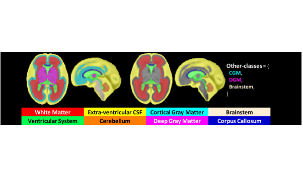
Figure 1: Illustration of partial annotations on a control fetal brain MRI [12]. b) all the leaf-labels are annotated. c) partial annotations where cortical gray matter (CGM), deep gray matter (DGM), and brainstem (B) are not annotated. In this cases, unannotated voxels have the label-set annotation {CGM, DGM, B}.

In fully-supervised learning, we learn from ground-truth segmentations $\textbf{g}\in\mathbf{L}^{N}$ where $N$ is the number of voxels and $\mathbf{L}$ is the set of final labels (e.g. white matter, ventricular system). We denote elements of $\mathbf{L}$ as leaf-labels. In contrast, with partial supervision, $\textbf{g}\in\left(2^{\mathbf{L}}\right)^{N}$, where $2^{\mathbf{L}}$ is the set of subsets of $\mathbf{L}$. In other words, each voxel annotation is a set of leaf-labels (a label-set). The label-set of an annotated white matter voxel would be simply {white matter}, and the label-set of a voxel that could be either white matter or deep gray matter would be {white matter, deep gray matter}. In both fully-supervised and partially-supervised learning, the network is trained to perform full segmentation predictions: $\textbf{p}\in{P\left(\mathbf{L}\right)^{N}}$, where $P(\mathbf{L})$ is the space of probability vectors for leaf-labels.

2.1 Label-set Loss Functions

A loss function $\mathcal{L}_{partial}(\cdot,\cdot)$ for partially supervised learning can be any differentiable function that compares a proposed probabilistic network output for leaf-labels, $\textbf{p}\in{P\left(\mathbf{L}\right)^{N}}$, and a partial label-set ground-truth annotation, $\textbf{g}\in{\left(2^{\mathbf{L}}\right)^{N}}$,

$$\begin{split}\mathcal{L}_{partial}:\,\,&{P\left(\mathbf{L}\right)^{N}}\times{\left(2^{\mathbf{L}}\right)^{N}}\xrightarrow{}\mathds{R}\\ \end{split}$$ (1)

However, such $\mathcal{L}_{partial}$, in general, may consider all possible label-sets as independent and ignore the relationship between a label-set and its constituent leaf-labels. We claim that segmentation loss functions for partially supervised learning must be compatible with the semantic of label-set inclusion. For example, in the case of three leaf-labels $\textbf{L}=\{l_{1},l_{2},l_{3}\}$, let voxel $i$ be labeled with the label-set $g_{i}=\{l_{1},l_{2}\}$. We know that the true leaf-label is either $l_{1}$ or $l_{2}$. Therefore the exemplar leaf-label probability vectors $\textbf{p}_{i}=(0.4,0.4,0.2)$, $\textbf{q}_{i}=(0.8,0,0.2)$, and $\textbf{h}_{i}=(0,0.8,0.2)$ need to be equivalent conditionally to the ground-truth partial annotation $g_{i}$. That is, the value of the loss function should be the same whether the predicted leaf-label probability vector for voxel $i$ is $\textbf{p}_{i}$, $\textbf{q}_{i}$, or $\textbf{h}_{i}$.

Formally, let us define the marginalization function $\Phi$ as

$$\begin{split}\Phi:\,\,&P\left(\mathbf{L}\right)^{N}\times\left(2^{\mathbf{L}}\right)^{N}\xrightarrow{}P\left(\mathbf{L}\right)^{N}\\ &(\textbf{p},\textbf{g})\mapsto(\tilde{p}_{i,c})\end{split}\,\,\textup{s.t.}\quad\forall i,c,\,\left\{\begin{array}[]{cc}\tilde{p}_{i,c}=\frac{1}{|g_{i}|}\sum_{c^{\prime}\in g_{i}}p_{i,c^{\prime}}&\textup{if}\,\,c\in g_{i}\\ \tilde{p}_{i,c}=p_{i,c}&\textup{if}\,\,c\not\in g_{i}\end{array}\right.$$

In the previous example, $\Phi(\textbf{p};\textbf{g})_{i}=\Phi(\textbf{q};\textbf{g})_{i}=\Phi(\textbf{h};\textbf{g})_{i}=(0.4,0.4,0.2).$ We define label-set loss functions as the functions $\mathcal{L}_{partial}$ that satisfy the axiom

$$\forall\textbf{g},\forall\textbf{p},\textbf{q},\quad\Phi(\textbf{p};\textbf{g})=\Phi(\textbf{q};\textbf{g})\implies\mathcal{L}_{partial}(\textbf{p},\textbf{g})=\mathcal{L}_{partial}(\textbf{q},\textbf{g})$$ (2)

We demonstrate that a loss $\mathcal{L}$ is a label-set loss function if and only if

$$\forall(\textbf{p},\textbf{g}),\quad\mathcal{L}(\textbf{p},\textbf{g})=\mathcal{L}\left(\Phi(\textbf{p};\textbf{g}),\textbf{g}\right)$$ (3)

See the supplementary material for a proof of this equivalence.

2.2 Leaf-Dice: A Label-set Generalization of the Dice Loss

In this section, as per previous work [5, 6, 8, 21, 23, 26], we consider the particular case in which, per training example, there is only one label-set that is not a singleton and contains all the leaf-labels that were not manually segmented in this example. An illustration for fetal brain segmentation can be found in Fig.1.

We propose a generalization of the mean class Dice Loss [10, 15] for this particular case and prove that it satisfies our axiom (2).

Let $\textbf{g}\in{\left(2^{\mathbf{L}}\right)^{N}}$ be a partial label-set segmentation such that there exists a label-set $\mathbf{L}_{\textbf{g}}^{\prime}\subsetneq\mathbf{L}$ that contains all the leaf-labels that were not manually segmented for this subject. Therefore, g takes its values in $\{\mathbf{L}_{\textbf{g}}^{\prime}\}\cup\left\{\{c\}\,|\,c\in\mathbf{L}\setminus\mathbf{L}_{\textbf{g}}^{\prime}\right\}$. We demonstrate that the leaf-Dice loss defined below is a label-set loss function

$$\forall\textbf{p},\quad\mathcal{L}_{Leaf-Dice}(\textbf{p},\textbf{g})=1-\frac{1}{|\mathbf{L}|}\sum_{c\in\mathbf{L}}\frac{2\sum_{i}\mathds{1}(g_{i}=\{c\})\,p_{i,c}}{\sum_{i}\mathds{1}(g_{i}=\{c\})^{\alpha}+\sum_{i}p_{i,c}^{\alpha}+\epsilon}$$ (4)

where $\alpha\in\{1,2\}$ (in line with the variants of soft Dice encountered in practice), and $\epsilon>0$ is a small constant. A proof that $\mathcal{L}_{Leaf-Dice}$ satisfies (3) can be found in the supplementary material. It is worth noting that using $\mathcal{L}_{Leaf-Dice}$ is not equivalent to just masking out the unannotated voxels, i.e. the voxels $i$ such that $g_{i}=\mathbf{L^{\prime}}_{\textbf{g}}$. Indeed, for all the $c\in\mathbf{L}\setminus\mathbf{L}_{\textbf{g}}^{\prime}$, the term $\sum_{i}p_{i,c}^{\alpha}$ in the denominator pushes $p_{i,c}$ towards $0$ for all the voxels indices $i$ including the indices $i$ for which $g_{i}=\mathbf{L}_{\textbf{g}}^{\prime}$. As a result, when $g_{i}=\mathbf{L}_{\textbf{g}}^{\prime}$, only the $p_{i,c}^{\alpha}$ for $c\not\in\mathbf{L}_{\textbf{g}}^{\prime}$ are pushed toward $0$, which in return pushes the $p_{i,c}^{\alpha}$ for $c\in\mathbf{L}_{\textbf{g}}^{\prime}$ towards $1$ since $\sum_{c\in\mathbf{L}}p_{i,c}=1$.

2.3 Converting Classical Loss Functions to Label-set Loss Functions

In this section, we demonstrate that there is one and only one canonical method to convert a segmentation loss function for fully supervised learning into a label-set loss function for partially supervised learning satisfying (3).

Formally, a label-set segmentation g can be seen as a soft segmentation using an injective function $\Psi:\left(2^{\mathbf{L}}\right)^{N}\hookrightarrow{}P\left(\mathbf{L}\right)^{N}$ that satisfies the relation

$$\forall\textbf{g}\in{\left(2^{\mathbf{L}}\right)^{N}},\,\forall i,c,\quad[\Psi(\textbf{g})]_{i,c}>0\implies c\in g_{i}$$ (5)

Note however, that the function $\Psi$ is not unique. Following the maximum entropy principle leads to choose

$$\Psi_{0}:(g_{i})\mapsto(\tilde{p}_{i,c})\quad\textup{s.t.}\quad\forall i,c\,\left\{\begin{array}[]{cc}\tilde{p}_{i,c}=\frac{1}{|g_{i}|}&\textup{if}\,\,c\in g_{i}\\ \tilde{p}_{i,c}=0&\textup{otherwise}\end{array}\right.$$ (6)

We are interested in converting a loss function for fully-supervised learning $\mathcal{L}_{fully}:\,\,P\left(\mathbf{L}\right)^{N}\times P\left(\mathbf{L}\right)^{N}\xrightarrow{}\mathds{R}$ into a label-set loss function for partial supervision defined as $\mathcal{L}_{partial}(\textbf{p},\textbf{g})=\mathcal{L}_{fully}(\textbf{p},\Psi\left(\textbf{g}\right))$.

Assuming that $\mathcal{L}_{fully}$ is minimal if and only if the predicted segmentation and the soft ground-truth segmentation are equal, we demonstrate in the supplementary material that $\mathcal{L}_{partial}$ is a label-set loss function if and only if

$$\forall(\textbf{p},\textbf{g})\in{P\left(\mathbf{L}\right)^{N}}\times{\left(2^{\mathbf{L}}\right)^{N}},\quad\left\{\begin{aligned} \mathcal{L}_{partial}(\textbf{p},\textbf{g})&=\mathcal{L}_{fully}\left(\Phi(\textbf{p};\textbf{g}),\Psi(\textbf{g})\right)\\ \Psi(\textbf{g})&=\Psi_{0}(\textbf{g})\end{aligned}\right.$$ (7)

Therefore, the only way to convert a fully-supervised loss to a loss for partially-supervised learning that complies with our axiom (2) is to use the marginalization function $\Phi$ on the predicted segmentation and $\Psi_{0}$ on the ground-truth partial segmentation. For clarity, we emphasise that the Leaf-Dice is a generalisation rather than a conversion of the Dice loss.

Related Work. When $\mathcal{L}_{fully}$ is the mean class Dice loss [10, 15] and the values of g are a partition of $\mathbf{L}$, like in section 2.2, one can prove that $\mathcal{L}_{partial}$ is the marginal Dice loss [23] (proof in supplementary material). Similarly, when $\mathcal{L}_{fully}$ is the cross entropy loss, $\mathcal{L}_{partial}$ is the marginal cross entropy loss [8, 21, 23]. Note that in [8, 21, 23], the marginalization approach is proposed as a possible method to convert the loss function. We prove that this is the only method.

3 Fetal Brain 3D MRI Data with Partial Segmentations

In this section, we describe the fetal brain 3D MRI datasets that were used.

Table 1: Number of 3D MRI and number of manual segmentations available per tissue types. WM: white matter, Vent: ventricular system, Cer: cerebellum, ECSF: extra-ventricular CSF, CGM: cortical gray matter, DGM: deep gray matter, BS: brainstem, CC: corpus callosum.

Train/Test	Condition	MRI	WM	Vent	Cer	ECSF	CGM	DGM	BS	CC
Training	Atlas [12]	18	18	18	18	18	18	18	18	18
Training	Controls	116	116	116	116	54	0	0	0	18
Training	Spina Bifida	30	30	30	30	0	0	0	0	0
Testing	Controls	34	34	34	34	34	15	15	15	0
Testing	Spina Bifida	66	66	66	66	66	25	25	25	41

Training Data for Fully Supervised Learning: $18$ fully-annotated control fetal brain MRI from a spatio-temporal [12].

Training Data for Partially Supervised Learning: $18$ fully-annotated volumes from the fully-supervised dataset, combined with $146$ partially annotated fetal brain MRI from a private dataset. The segmentations available for those 3D MRI are detailed in Table 1.

Multi-centric Testing Data: $100$ fetal brain 3D MRI. This includes $60$ volumes from University Hospital Leuven and $40$ volumes from the publicly available FeTA dataset [17]. The segmentations available for those 3D MRI are detailed in Table 1. The 3D MRI of the FeTA dataset come from a different center than the training data. Automatic brain masks for the FeTA data were obtained using atlas affine registration with a normal fetal brain and a spina bifida spatio-temporal atlas [11, 12].

Image Acquisition and Preprocessing for the Private Dataset. All images were part of routine clinical care and were acquired at University Hospital Leuven. In total, 74 cases with open spina bifida and 135 cases with normal brains, referred as controls, were included. Three spina bifida cases have been excluded by a pediatric radiologist because the quality of the 2D MRI resulted in corrupted 3D MRI which did not allow accurate segmentation. The gestational age at MRI ranged from $20$ weeks to $35$ weeks (median=$26.9$ weeks, IQR=$3.4$ weeks). For each study, at least three orthogonal T2-weighted HASTE series of the fetal brain were collected on a $1.5$T scanner using an echo time of $133$ms, a repetition time of $1000$ms, with no slice overlap nor gap, pixel size $0.39$mm to $1.48$mm, and slice thickness $2.50$mm to $4.40$mm. A radiologist attended all the acquisitions for quality control. The fetal brain 3D MRI were obtained using NiftyMIC [7] a state-of-the-art super resolution and reconstruction algorithm. The volumes were all reconstructed to a resolution of $0.8$ mm isotropic and registered to a standard clinical view. NiftyMIC also outputs brain masks that were used to define the label-sets and to mask the background [20].

Labelling Protocol. The labelling protocol is the same as in [17]. The different tissue types were segmented by a trained obstetrician and medical students under the supervision of a paediatric radiologist specialized in fetal brain anatomy, who quality controlled and corrected all manual segmentations. The voxels inside the brain mask that were not annotated by experts were assigned to the label-set containing all the tissue types that were not annotated for the 3D MRI. It is assumed that the voxels that were not annotated by experts were correctly not annotated.

4 Experiments

In this section, we compare three partially supervised methods and one fully supervised method using the fetal brain 3D MRI dataset described in section 3.

Figure 2: Qualitative comparison on an open spina bifida case. Only the proposed Leaf-Dice loss provides satisfactory segmentations for all tissue types.

Deep Learning Pipeline. We use a 3D U-Net [3] architecture with $5$ levels, leaky ReLU and instance normalization [24]. For training and inference, the entire volumes were used as input of the 3D U-Net after padding to $144\times 160\times 144$ voxels. For each method of Table 2, an ensemble of $10$ 3D U-Net is used. Using an ensemble of models makes the comparison of segmentation results across methods less sensitive to the random initialization of each network. Each 3D U-Net is trained using a random split of the training dataset into $90\%$ for training and $10\%$ for early stopping. During training, we used a batch size of $3$, a learning rate of $0.001$, and Adam [14] optimizer with default hyperpameter values. The learning rate was tuned for the fully supervised learning baseline. Random right/left flip, random scaling, gamma intensity augmentation, contrast augmentation, and additive Gaussian noise were used as data augmentation during training. Our code for the label-set loss functions and the deep learning pipeline are publicly available^,.

Hardware. For training we used NVIDIA Tesla V100 GPUs. Training each model took from one to two days. For inference, we used a NVIDIA GTX 1070 GPU. The inference for a 3D MRI takes between one and two minutes.

Specificities of Each Method. Baseline 1 is trained using fully supervised learning, the mean class Dice loss [10, 15], referred as $\mathcal{L}_{Dice}$, and the training dataset for fully supervised learning of Section 3 (18 training volumes only). The three other methods are trained using partially supervised learning and the training dataset for partially supervised learning of Section 3. Baseline 2 is trained using the soft-target Dice loss function defined as $\mathcal{L}_{Dice}(\textbf{p},\Psi_{0}(\textbf{g}))$, where $\Psi_{0}$ is defined in (6). Note that Baseline 2 does not satisfy the label-set axiom (2). Baseline 3 is trained using the marginal Dice loss [23]. Our method is trained using the proposed Leaf-Dice loss defined in (4). The loss functions of Baseline 3 and our method satisfy the axiom of label-set loss functions (2).

Statistical Analysis. We used the two-sided Wilcoxon signed-rank test. Differences in mean values are considered significant when $p<0.01$.

Table 2: Evaluation on the Multi-centric Testing Data (100 3D MRI).

We report mean (standard deviation) for the Dice score (DSC) in percentages and the Hausdorff distance at $95\%$ (HD95) in millimeters for the eight tissue types. Methods underlined are trained using partially supervised learning. Loss functions in bold satisfy the axiom of label-set loss functions. Best mean values are in bold. Mean values significantly better with $p<0.01$ (resp. worse) than the ones achieved by the fully-supervised learning baseline are marked with a $*$ (resp. a ${\dagger}$). Model Metric WM Vent Cer ECSF CGM DGM BS CC Baseline 1 DSC 76.4 (12.5) 72.1 (18.8) 67.3 (28.6) 63.9 (31.3) 47.3 (10.9) 72.7 (8.7) 56.0 (27.7) 51.6 (10.5) Fully-Supervised HD95 3.3 (1.2) 4.8 (3.7) 4.9 (5.2) 7.3 (7.8) 5.3 (0.9) 5.8 (2.1) 9.1 (8.2) 5.1 (3.1) Baseline 2 DSC $89.5^{*}$ (6.5) $87.5^{*}$ (9.6) $87.2^{*}$ (10.3) $37.7^{{\dagger}}$ (34.2) $31.4^{{\dagger}}$ (14.8) $18.2^{{\dagger}}$ (20.5) $20.2^{{\dagger}}$ (13.1) $12.0^{{\dagger}}$ (10.8) Soft-target Dice HD95 $1.7^{*}$ (1.3) $1.6^{*}$ (2.2) $2.2^{*}$ (4.5) 7.1 (6.8) $6.2^{{\dagger}}$ (2.0) $24.2^{{\dagger}}$ (9.0) $33.9^{{\dagger}}$ (5.9) $29.3^{{\dagger}}$ (8.0) Baseline 3 [23] DSC $89.6^{*}$ (6.7) $87.7^{*}$ (10.4) $87.6^{*}$ (9.5) $66.6^{*}$ (27.7) 43.9 (15.1) $37.8^{{\dagger}}$ (11.3) $39.4^{{\dagger}}$ (16.8) $11.1^{{\dagger}}$ (12.3) Marginal Dice HD95 $1.7^{*}$ (1.3) $1.6^{*}$ (2.2) $2.4^{*}$ (5.4) $6.2^{*}$ (7.6) $4.4^{*}$ (1.4) $26.7^{{\dagger}}$ (6.7) $33.4^{{\dagger}}$ (6.1) $28.7^{{\dagger}}$ (6.3) Ours DSC $\bf 91.5^{*}$ (6.7) $\bf 90.7^{*}$ (8.9) $\bf 89.6^{*}$ (10.1) $\bf 75.3^{*}$ (24.9) $\bf 56.6^{*}$ (14.3) 71.4 (8.6) $\bf 61.5^{*}$ (21.7) $\bf 62.0^{*}$ (10.9) Leaf-Dice HD95 $\bf 1.5^{*}$ (1.1) $\bf 1.4^{*}$ (2.0) $\bf 1.7^{*}$ (1.8) $\bf 5.4^{*}$ (8.3) $\bf 3.9^{*}$ (1.3) $7.3^{{\dagger}}$ (2.3) $\bf 7.9$ (4.0) $\bf 2.9^{*}$ (1.5)

Comparison of Fully Supervised and Partially Supervised Learning. The quantitative evaluation can be found in Table 2. The partially supervised learning methods of Table 2 all perform significantly better than the fully supervised learning baseline in terms of Dice score and Hausdorff distance on the tissue types for which annotations are available for all the training data of Table 1, i.e. white matter, ventricles, and cerebellum. Some tissue types segmentations are scarce in the partially supervised training dataset as can be seen in Table 1, i.e. cortical gray matter, deep gray matter, brainstem, and corpus callosum. This makes it challenging for partially supervised methods to learn to segment those tissue types. Only Leaf-Dice achieves similar or better segmentation results than the fully supervised baseline for the scarce tissue types, except in terms of Hausdorff distance for the deep gray matter. The extra-ventricular CSF is an intermediate case with almost half the data annotated. The Leaf-Dice and the Marginalized Dice significantly outperforms the fully supervised baseline for all metrics for the extra-ventricular CSF, and the soft-target Dice performs significantly worse than this baseline.

Comparison of Loss Functions for Partially Supervised Learning. The Leaf-Dice performs significantly better than the soft-target Dice for all tissue types and all metrics. The Marginal Dice performs significantly better than the soft-target Dice in terms of Dice score for extra-ventricular CSF, cortical gray matter, deep gray matter, and brainstem. Since the soft-target Dice loss is the only loss that does not satisfy the proposed axiom for label-set loss functions, this suggests label-set loss functions satisfying our axiom perform better in practice.

In addition, our Leaf-Dice performs significantly better than the Marginal Dice [23] for all metrics and all tissue types. The qualitative results of Fig. 2 also suggest that Leaf-Dice performs better than the other approaches. This suggests that using a converted fully supervised loss function, as proposed in section 2.3 and in previous work [8, 21, 23], may be outperformed by dedicated generalised label-set loss functions.

5 Conclusion

In this work, we present the first axiomatic definition of label-set loss functions for training a deep learning model with partially segmented images. We propose a generalization of the Dice loss, Leaf-Dice, that complies with our axiom for the common case of missing labels that were not manually segmented. We prove that loss functions that were proposed in the literature for partially supervised learning satisfy the proposed axiom. In addition, we prove that there is one and only one way to convert a loss function for fully segmented images into a label-set loss function for partially segmented images.

We propose the first application of partially supervised learning to fetal brain 3D MRI segmentation. Our experiments illustrate the advantage of using partially segmented images in addition to fully segmented images. The comparison of our Leaf-Dice to three baselines suggests that label-set loss functions that satisfy our axiom perform significantly better for fetal brain 3D MRI segmentation.

Acknowledgments

This project has received funding from the European Union’s Horizon 2020 research and innovation program under the Marie Skłodowska-Curie grant agreement TRABIT No 765148. This work was supported by core and project funding from the Wellcome [203148/Z/16/Z; 203145Z/16/Z; WT101957], and EPSRC [NS/A000049/1; NS/A000050/1; NS/A000027/1]. TV is supported by a Medtronic / RAEng Research Chair [RCSRF1819\7\34].

1 Summary of mathematical notations

• $N$: number of voxels.

• $\mathbf{L}$: set of final labels (e.g. white matter, ventricular system). We call the elements of $\mathbf{L}$ leaf-labels.

• $2^{\mathbf{L}}$: set of subsets of $\mathbf{L}$ We call the elements of $2^{\mathbf{L}}$ label-sets.

• $P(\mathbf{L})$: space of probability vectors for leaf-labels.

• $\mathds{1}$: indicator function. let A an assertion, $\mathds{1}(A)=1$ if $A$ is true and $\mathds{1}(A)=0$ if $A$ is false.

2 Proof of equation (3)

Let $\mathcal{L}:\,\,\mathbf{E}\xrightarrow{}\mathds{R}$, with $\textbf{E}:=P\left(\mathbf{L}\right)^{N}\times\left(2^{\mathbf{L}}\right)^{N}$. Let us first remind that we have defined label-set loss functions as the losses $\tilde{\mathcal{L}}$ that satisfy the axiom

$$\forall\textbf{g}\in\left(2^{\mathbf{L}}\right)^{N},\,\forall\textbf{p},\textbf{q}\in P(\textbf{L})^{N},\quad\Phi(\textbf{p};\textbf{g})=\Phi(\textbf{q};\textbf{g})\implies\tilde{\mathcal{L}}(\textbf{p},\textbf{g})=\tilde{\mathcal{L}}(\textbf{q},\textbf{g})$$ (8)

First implication.

Let us assume that $\forall(\textbf{p},\textbf{g})\in\textbf{E},\,\,\mathcal{L}(\textbf{p},\textbf{g})=\mathcal{L}(\Phi(\textbf{p};\textbf{g}),\textbf{g})$. Let $\textbf{g}\in\left(2^{\mathbf{L}}\right)^{N}$ and $\textbf{p},\textbf{q}\in P(\textbf{L})^{N}$, such that $\Phi(\textbf{p};\textbf{g})=\Phi(\textbf{q};\textbf{g})$. We have

$$\mathcal{L}(\textbf{p},\textbf{g})=\mathcal{L}(\Phi(\textbf{p};\textbf{g}),\textbf{g})=\mathcal{L}(\Phi(\textbf{q};\textbf{g}),\textbf{g})=\mathcal{L}(\textbf{q},\textbf{g})\,\,\blacksquare$$

Second implication.

Let us assume that $\mathcal{L}$ is a label-set loss function. We will use the following lemma which is proved at the end of this paragraph.

Lemma 1

For all $\textbf{g}\in\left(2^{\mathbf{L}}\right)^{N}$, the function $\Phi(\cdot\,;\textbf{g}):\textbf{p}\mapsto\Phi(\textbf{p};\textbf{g})$ is idempotent, i.e. $\forall\textbf{p}\in P(\mathbf{L})^{N},\,\Phi(\Phi(\textbf{p};\textbf{g});\textbf{g})=\Phi(\textbf{p};\textbf{g})$.

Let $(\textbf{p},\textbf{g})\in\textbf{E}$. By Lemma 1, $\Phi(\Phi(\textbf{p};\textbf{g});\textbf{g})=\Phi(\textbf{p};\textbf{g}).$ Therefore, by applying (8) for p and $\textbf{q}=\Phi(\textbf{p};\textbf{g})$ we eventually obtain $\mathcal{L}(\textbf{p},\textbf{g})=\mathcal{L}(\Phi(\textbf{p};\textbf{g}),\textbf{g})$ $\blacksquare$

Proof of Lemma 1

Let $\textbf{g}=(g_{i})\in\left(2^{\mathbf{L}}\right)^{N}$ and $\textbf{p}=(p_{i,c})\in P(\textbf{L})^{N}$. Let us denote $\Phi(\textbf{p};\textbf{g})=(\tilde{p}_{i,c})$ and $\Phi(\Phi(\textbf{p};\textbf{g});\textbf{g})=(\tilde{\raisebox{0.0pt}[0.85pt]{$\tilde{p}$}}_{i,c})$. For all $i,c$, if $c\not\in g_{i}$, $\tilde{\raisebox{0.0pt}[0.85pt]{$\tilde{p}$}}_{i,c}=\tilde{p}_{i,c}$, and if $c\in g_{i}$, $\tilde{\raisebox{0.0pt}[0.85pt]{$\tilde{p}$}}_{i,c}=\frac{1}{|g_{i}|}\sum_{c^{\prime}\in g_{i}}\tilde{p}_{i,c^{\prime}}=\frac{1}{|g_{i}|}\sum_{c^{\prime}\in g_{i}}\left(\frac{1}{|g_{i}|}\sum_{c^{\prime\prime}\in g_{i}}p_{i,c^{\prime\prime}}\right)=\tilde{p}_{i,c}$ $\blacksquare$

3 Proof that the leaf-Dice is a label-set loss function

Let $\textbf{g}\in{\left(2^{\mathbf{L}}\right)^{N}}$ be a partial segmentation that takes its value in a partition of $\mathbf{L}$ of the form $\{\mathbf{L}^{\prime}\}\cup\left\{\{c\}\,|\,c\in\mathbf{L}\setminus\mathbf{L}^{\prime}\right\}$ with $\mathbf{L}^{\prime}\subsetneq\mathbf{L}$ that contains all the labels of the regions of interest that were not manually segmented. Let $\textbf{p}\in{P\left(\mathbf{L}\right)^{N}}$.

$$\begin{split}\mathcal{L}_{Leaf-Dice}(\textbf{p},\textbf{g})&=1-\frac{1}{|\mathbf{L}|}\sum_{c\in\mathbf{L}}\frac{2\sum_{i}\mathds{1}(g_{i}=\{c\})\,p_{i,c}}{\sum_{i}\mathds{1}(g_{i}=\{c\})^{\alpha}+\sum_{i}p_{i,c}^{\alpha}+\epsilon}\\ &=1-\frac{1}{|\mathbf{L}|}\sum_{c\in\mathbf{L}\setminus\mathbf{L}^{\prime}}\frac{2\sum_{i}\mathds{1}(g_{i}=\{c\})\,p_{i,c}}{\sum_{i}\mathds{1}(g_{i}=\{c\})^{\alpha}+\sum_{i}p_{i,c}^{\alpha}+\epsilon}\end{split}$$ (9)

because the terms of the sum for the leaf-labels $c\in\mathbf{L}^{\prime}$ have a numerator equal to $0$.

To prove that $\mathcal{L}_{Leaf-Dice}$ is a label-set loss function it is sufficient to prove that $\mathcal{L}_{Leaf-Dice}(\textbf{p},\textbf{g})=\mathcal{L}_{Leaf-Dice}(\Phi(\textbf{p;{g}}),\textbf{g}).$ For all voxel i and leaf-label c

$$\left[\Phi(\textbf{p;{g}})\right]_{i,c}=\left\{\begin{array}[]{cc}\frac{1}{|g_{i}|}\sum_{c^{\prime}\in g_{i}}p_{i,c^{\prime}}&\textup{if}\,\,c\in g_{i}\\ p_{i,c}&\textup{if}\,\,c\not\in g_{i}\end{array}\right.=\left\{\begin{array}[]{cc}\frac{1}{|\mathbf{L}^{\prime}|}\sum_{c^{\prime}\in\mathbf{L}^{\prime}}p_{i,c^{\prime}}&\textup{if}\,\,c\in g_{i}\,\,\textup{and}\,\,g_{i}=\mathbf{L}^{\prime}\\ p_{i,c}&\textup{if}\,\,c\in g_{i}\,\,\textup{and}\,\,g_{i}=\{c\}\\ p_{i,c}&\textup{if}\,\,c\not\in g_{i}\end{array}\right.$$

where the second equality comes from the partition.

We observe that $\left[\Phi(\textbf{p;{g}})\right]_{i,c}\neq p_{i,c}$ only when $c\in\mathbf{L}^{\prime}$. Using (9) we obtain $\mathcal{L}_{Leaf-Dice}(\textbf{p},\textbf{g})=\mathcal{L}_{Leaf-Dice}(\Phi(\textbf{p;{g}}),\textbf{g})\,\blacksquare$

4 Proof of equation (7)

Using previous results and the fact that $\mathcal{L}_{partial}$ is here defined as a converted fully-supervised loss function, $\mathcal{L}_{partial}$ is a label-set loss function if and only if for all $(\textbf{p},\textbf{g})\in{P\left(\mathbf{L}\right)^{N}}\times{\left(2^{\mathbf{L}}\right)^{N}}$

$$\mathcal{L}_{partial}(\textbf{p},\textbf{g})=\mathcal{L}_{partial}(\Phi(\textbf{p};\textbf{g}),\textbf{g})=\mathcal{L}_{fully}(\Phi(\textbf{p};\textbf{g}),\Psi(\textbf{g}))$$

As a result, we only need to prove that if $\mathcal{L}_{partial}$ is a label-set loss function then $\Psi=\Psi_{0}$. Let us suppose that $\mathcal{L}_{partial}$ is a label-set loss function. Therefore, for all $\textbf{g}\in{\left(2^{\mathbf{L}}\right)^{N}},\,\,\mathcal{L}_{fully}(\Phi(\Psi(\textbf{g});\textbf{g}),\Psi(\textbf{g}))=\mathcal{L}_{partial}(\Phi(\Psi(\textbf{g});\textbf{g}),\textbf{g})=\mathcal{L}_{partial}(\Psi(\textbf{g}),\textbf{g})=\mathcal{L}_{fully}(\Psi(\textbf{g}),\Psi(\textbf{g})).$ Using the unicity of the minima of $\mathcal{L}_{fully}$ we can therefore conclude that $\forall\textbf{g}\in{\left(2^{\mathbf{L}}\right)^{N}},\,\,\Psi(\textbf{g})=\Phi(\Psi(\textbf{g});\textbf{g}).$ For all $\textbf{g},i,c$,

$$\left[\Phi(\Psi(\textbf{g});\textbf{g})\right]_{i,c}=\left\{\begin{array}[]{cc}\frac{1}{|g_{i}|}\sum_{c^{\prime}\in g_{i}}\left[\Psi(\textbf{g})\right]_{i,c^{\prime}}&\textup{if}\,\,c\in g_{i}\\ \left[\Psi(\textbf{g})\right]_{i,c}&\textup{if}\,\,c\not\in g_{i}\end{array}\right.=\left\{\begin{array}[]{cc}\frac{1}{|g_{i}|}&\textup{if}\,\,c\in g_{i}\\ 0&\textup{if}\,\,c\not\in g_{i}\end{array}\right.=\left[\Psi_{0}(\textbf{g})\right]_{i,c}$$

where in the second inequality we have used $\forall i,c,\,\,[\Psi(\textbf{g})]_{i,c}>0\implies c\in g_{i}\,\,\blacksquare$

5 Relation to the marginal Dice loss

Let $P=\{\mathbf{L}_{j}\}$ a partition of $\mathbf{L}$ and $\textbf{g}\in{\left(2^{\mathbf{L}}\right)^{N}}$ with its values in $P$. For all $c\in\mathbf{L}$, we denote $j(c)$ the unique index such that $c\in\mathbf{L}_{j(c)}$.

Using the definitions of $\Psi_{0}$, $\Phi$, and the partition $P$, we obtain

$$\begin{split}\mathcal{L}_{Dice}\left(\Phi(\textbf{p};\textbf{g}),\Psi_{0}(\textbf{g})\right)&=1-\frac{1}{|\mathbf{L}|}\sum_{c\in\mathbf{L}}\frac{\sum_{i}\Psi_{0}(\textbf{g})_{i,c}\Phi(\textbf{p};\textbf{g})_{i,c}}{\sum_{i}\Psi_{0}(\textbf{g})_{i,c}+\sum_{i}\Phi(\textbf{p};\textbf{g})_{i,c}}\\ &=1-\frac{1}{|\mathbf{L}|}\sum_{c\in\mathbf{L}}\frac{\sum_{i}\left(\frac{1}{|\mathbf{L}_{j(c)}|}\mathds{1}\left(g_{i}=\mathbf{L}_{j(c)}\right)\right)\left(\frac{1}{|\mathbf{L}_{j(c)}|}\sum_{c^{\prime}\in\mathbf{L}_{j(c)}}p_{i,c^{\prime}}\right)}{\sum_{i}\frac{1}{|\mathbf{L}_{j(c)}|}\mathds{1}\left(g_{i}=\mathbf{L}_{j(c)}\right)+\sum_{i}\frac{1}{|\mathbf{L}_{j(c)}|}\sum_{c^{\prime}\in\mathbf{L}_{j(c)}}p_{i,c^{\prime}}}\\ &=1-\frac{1}{|\mathbf{L}|}\sum_{c\in\mathbf{L}}\frac{\left(\frac{1}{|\mathbf{L}_{j(c)}|}\right)^{2}\sum_{i}\mathds{1}\left(g_{i}=\mathbf{L}_{j(c)}\right)\left(\sum_{c^{\prime}\in\mathbf{L}_{j(c)}}p_{i,c^{\prime}}\right)}{\frac{1}{|\mathbf{L}_{j(c)}|}\left(\sum_{i}\mathds{1}\left(g_{i}=\mathbf{L}_{j(c)}\right)+\sum_{i}\sum_{c^{\prime}\in\mathbf{L}_{j(c)}}p_{i,c^{\prime}}\right)}\\ &=1-\frac{1}{|\mathbf{L}|}\sum_{c\in\mathbf{L}}\frac{1}{|\mathbf{L}_{j(c)}|}\frac{\sum_{i}\mathds{1}\left(g_{i}=\mathbf{L}_{j(c)}\right)\left(\sum_{c^{\prime}\in\mathbf{L}_{j(c)}}p_{i,c^{\prime}}\right)}{\sum_{i}\mathds{1}\left(g_{i}=\mathbf{L}_{j(c)}\right)+\sum_{i}\sum_{c^{\prime}\in\mathbf{L}_{j(c)}}p_{i,c^{\prime}}}\\ \end{split}$$

By grouping the terms of the first sum with respect to the label-sets in $P$

$$\begin{split}\mathcal{L}_{Dice}\left(\Phi(\textbf{p};\textbf{g}),\Psi_{0}(\textbf{g})\right)&=1-\frac{1}{|\mathbf{L}|}\sum_{\mathbf{L}^{\prime}\in P}\sum_{c\in\mathbf{L}^{\prime}}\frac{1}{|\mathbf{L}_{j(c)}|}\frac{\sum_{i}\mathds{1}\left(g_{i}=\mathbf{L}_{j(c)}\right)\left(\sum_{c^{\prime}\in\mathbf{L}_{j(c)}}p_{i,c^{\prime}}\right)}{\sum_{i}\mathds{1}\left(g_{i}=\mathbf{L}_{j(c)}\right)+\sum_{i}\sum_{c^{\prime}\in\mathbf{L}_{j(c)}}p_{i,c^{\prime}}}\\ &=1-\frac{1}{|\mathbf{L}|}\sum_{\mathbf{L}^{\prime}\in P}\sum_{c\in\mathbf{L}^{\prime}}\frac{1}{|\mathbf{L}^{\prime}|}\frac{\sum_{i}\mathds{1}\left(g_{i}=\mathbf{L}^{\prime}\right)\left(\sum_{c^{\prime}\in\mathbf{L}^{\prime}}p_{i,c^{\prime}}\right)}{\sum_{i}\mathds{1}\left(g_{i}=\mathbf{L}^{\prime}\right)+\sum_{i}\sum_{c^{\prime}\in\mathbf{L}^{\prime}}p_{i,c^{\prime}}}\\ &=1-\frac{1}{|\mathbf{L}|}\sum_{\mathbf{L}^{\prime}\in P}\frac{\sum_{i}\mathds{1}\left(g_{i}=\mathbf{L}^{\prime}\right)\left(\sum_{c^{\prime}\in\mathbf{L}^{\prime}}p_{i,c^{\prime}}\right)}{\sum_{i}\mathds{1}\left(g_{i}=\mathbf{L}^{\prime}\right)+\sum_{i}\sum_{c^{\prime}\in\mathbf{L}^{\prime}}p_{i,c^{\prime}}}\\ \end{split}$$

because for all $\mathbf{L}^{\prime}\in P$ and all $c\in\mathbf{L}^{\prime}$, $\mathbf{L}_{j(c)}=\mathbf{L}^{\prime}$.

The right hand-side of the last equality is the marginal Dice loss [23] up to the multiplicative constant $\frac{1}{|\mathbf{L}|}$ $\blacksquare$

References

- [1] Aertsen, M., Verduyckt, J., De Keyzer, F., Vercauteren, T., Van Calenbergh, F., De Catte, L., Dymarkowski, S., Demaerel, P., Deprest, J.: Reliability of MR imaging–based posterior fossa and brain stem measurements in open spinal dysraphism in the era of fetal surgery. American Journal of Neuroradiology 40(1), 191–198 (2019)
- [2] Benkarim, O.M., Sanroma, G., Zimmer, V.A., Muñoz-Moreno, E., Hahner, N., Eixarch, E., Camara, O., Gonzalez Ballester, M.A., Piella, G.: Toward the automatic quantification of in utero brain development in 3D structural MRI: A review. Human brain mapping 38(5), 2772–2787 (2017)
- [3] Çiçek, Ö., Abdulkadir, A., Lienkamp, S.S., Brox, T., Ronneberger, O.: 3D U-Net: learning dense volumetric segmentation from sparse annotation. In: International conference on medical image computing and computer-assisted intervention. pp. 424–432. Springer (2016)
- [4] Danzer, E., Joyeux, L., Flake, A.W., Deprest, J.: Fetal surgical intervention for myelomeningocele: lessons learned, outcomes, and future implications. Developmental Medicine & Child Neurology 62(4), 417–425 (2020)
- [5] Dmitriev, K., Kaufman, A.E.: Learning multi-class segmentations from single-class datasets. In: Proceedings of the IEEE/CVF Conference on Computer Vision and Pattern Recognition. pp. 9501–9511 (2019)
- [6] Dorent, R., Booth, T., Li, W., Sudre, C.H., Kafiabadi, S., Cardoso, J., Ourselin, S., Vercauteren, T.: Learning joint segmentation of tissues and brain lesions from task-specific hetero-modal domain-shifted datasets. Medical Image Analysis 67, 101862 (2021)
- [7] Ebner, M., Wang, G., Li, W., Aertsen, M., Patel, P.A., Aughwane, R., Melbourne, A., Doel, T., Dymarkowski, S., De Coppi, P., et al.: An automated framework for localization, segmentation and super-resolution reconstruction of fetal brain MRI. NeuroImage 206, 116324 (2020)
- [8] Fang, X., Yan, P.: Multi-organ segmentation over partially labeled datasets with multi-scale feature abstraction. IEEE Transactions on Medical Imaging 39(11), 3619–3629 (2020)
- [9] Fetit, A.E., Alansary, A., Cordero-Grande, L., Cupitt, J., Davidson, A.B., Edwards, A.D., Hajnal, J.V., Hughes, E., Kamnitsas, K., Kyriakopoulou, V., et al.: A deep learning approach to segmentation of the developing cortex in fetal brain mri with minimal manual labeling. In: Medical Imaging with Deep Learning. pp. 241–261. PMLR (2020)
- [10] Fidon, L., Li, W., Garcia-Peraza-Herrera, L.C., Ekanayake, J., Kitchen, N., Ourselin, S., Vercauteren, T.: Generalised wasserstein dice score for imbalanced multi-class segmentation using holistic convolutional networks. In: International MICCAI Brainlesion Workshop. pp. 64–76. Springer (2017)
- [11] Fidon, L., Viola, E., Mufti, N., David, A., Melbourne, A., Demaerel, P., Ourselin, S., Vercauteren, T., Deprest, J., Aertsen, M.: A spatio-temporal atlas of the developing fetal brain with spina bifida aperta. Open Research Europe (2021)
- [12] Gholipour, A., Rollins, C.K., Velasco-Annis, C., Ouaalam, A., Akhondi-Asl, A., Afacan, O., Ortinau, C.M., Clancy, S., Limperopoulos, C., Yang, E., et al.: A normative spatiotemporal MRI atlas of the fetal brain for automatic segmentation and analysis of early brain growth. Scientific reports 7(1), 1–13 (2017)
- [13] Khalili, N., Lessmann, N., Turk, E., Claessens, N., de Heus, R., Kolk, T., Viergever, M., Benders, M., Išgum, I.: Automatic brain tissue segmentation in fetal MRI using convolutional neural networks. Magnetic resonance imaging 64, 77–89 (2019)
- [14] Kingma, D.P., Ba, J.: Adam: A method for stochastic optimization. arXiv preprint arXiv:1412.6980 (2014)
- [15] Milletari, F., Navab, N., Ahmadi, S.A.: V-net: Fully convolutional neural networks for volumetric medical image segmentation. In: 2016 fourth international conference on 3D vision (3DV). pp. 565–571. IEEE (2016)
- [16] Moise Jr, K.J., Moldenhauer, J.S., Bennett, K.A., Goodnight, W., Luks, F.I., Emery, S.P., Tsao, K., Moon-Grady, A.J., Moore, R.C., Treadwell, M.C., et al.: Current selection criteria and perioperative therapy used for fetal myelomeningocele surgery. Obstetrics & Gynecology 127(3), 593–597 (2016)
- [17] Payette, K., de Dumast, P., Kebiri, H., Ezhov, I., Paetzold, J.C., Shit, S., Iqbal, A., Khan, R., Kottke, R., Grehten, P., et al.: A comparison of automatic multi-tissue segmentation methods of the human fetal brain using the FeTA dataset. arXiv preprint arXiv:2010.15526 (2020)
- [18] Payette, K., Kottke, R., Jakab, A.: Efficient multi-class fetal brain segmentation in high resolution mri reconstructions with noisy labels. In: Medical Ultrasound, and Preterm, Perinatal and Paediatric Image Analysis, pp. 295–304. Springer (2020)
- [19] Payette, K., Moehrlen, U., Mazzone, L., Ochsenbein-Kölble, N., Tuura, R., Kottke, R., Meuli, M., Jakab, A.: Longitudinal analysis of fetal MRI in patients with prenatal spina bifida repair. In: Smart Ultrasound Imaging and Perinatal, Preterm and Paediatric Image Analysis, pp. 161–170. Springer (2019)
- [20] Ranzini, M., Fidon, L., Ourselin, S., Modat, M., Vercauteren, T.: MONAIfbs: MONAI-based fetal brain MRI deep learning segmentation. arXiv preprint arXiv:2103.13314 (2021)
- [21] Roulet, N., Slezak, D.F., Ferrante, E.: Joint learning of brain lesion and anatomy segmentation from heterogeneous datasets. In: International Conference on Medical Imaging with Deep Learning. pp. 401–413. PMLR (2019)
- [22] Sacco, A., Ushakov, F., Thompson, D., Peebles, D., Pandya, P., De Coppi, P., Wimalasundera, R., Attilakos, G., David, A.L., Deprest, J.: Fetal surgery for open spina bifida. The Obstetrician & Gynaecologist 21(4), 271 (2019)
- [23] Shi, G., Xiao, L., Chen, Y., Zhou, S.K.: Marginal loss and exclusion loss for partially supervised multi-organ segmentation. Medical Image Analysis p. 101979 (2021)
- [24] Ulyanov, D., Vedaldi, A., Lempitsky, V.: Instance normalization: The missing ingredient for fast stylization. arXiv preprint arXiv:1607.08022 (2016)
- [25] Zarutskie, A., Guimaraes, C., Yepez, M., Torres, P., Shetty, A., Sangi-Haghpeykar, H., Lee, W., Espinoza, J., Shamshirsaz, A., Nassr, A., et al.: Prenatal brain imaging for predicting need for postnatal hydrocephalus treatment in fetuses that had neural tube defect repair in utero. Ultrasound in Obstetrics & Gynecology 53(3), 324–334 (2019)
- [26] Zhou, Y., Li, Z., Bai, S., Wang, C., Chen, X., Han, M., Fishman, E., Yuille, A.L.: Prior-aware neural network for partially-supervised multi-organ segmentation. In: Proceedings of the IEEE/CVF International Conference on Computer Vision. pp. 10672–10681 (2019)
— Supplemental Document —