Molecular Communication with Passive Receivers in Anomalous Diffusion Channels

Abstract

We consider anomalous diffusion for molecular communication with a passive receiver. We first consider the probability density function of molecules’ location at a given time in a space of arbitrary dimension. The expected number of observed molecules inside a receptor space of the receiver at certain time is derived taking into account the life expectancy of the molecules. In addition, an implicit solution for the time that maximizes the expected number of observed molecules is obtained in terms of Fox’s $H$-function. The closed-form expressions for the bit error rate of a single-bit interval transmission and a multi-bit interval transmission are derived. It is shown that lifetime limited molecules can reduce the inter-symbol interference while also enhancing the reliability of MC systems at a suitable observation time.

I Introduction

Molecular communication (MC) is a new communication paradigm that uses tiny-machines which are nanometers to micrometers in size as a transmitter, a receiver, and molecules as a communication carrier [1]. Brownian motion (normal diffusion) which describes the free movement of molecules in a fluid medium is usually well adopted as an ideal diffusion scheme in MC. However, we may encounter extraordinary diffusion or anomalous diffusion, which does not obey normal diffusion principles, in crowded, heterogeneous, complex structure environments or the Brownian motion in an inhomogeneous medium [2, 3, 4]. Thus, anomalous diffusion has been paid more attention in recent studies on MC for various potential applications of MCs. MC under anomalous diffusion law in a $1$-dimensional ($1$-D) channel was first considered in [5]. In [6], the authors developed a connectivity model with random time constraints in a $1$-D mobile MC system. The network performance on the error probability in a $2$-D stochastic nanonetwork was investigated in [7]. $3$-D concentration-encoded subdiffusive MC and $3$-D subdiffusive MC with an absorbing receiver were considered in [8] and [9], respectively. Additionally, a new mathematical framework for the modeling and analysis of molecular communication under anomalous diffusion was developed in [10]. However, most of the studies have focused on analyzing the communication performance of MC with an absorbing receiver, that is, an active reception process is considered.

Normal diffusion-based MC with a receptor space (RS) where a receive nanomachine (or a nanosensor) is located inside the RS was considered in $1$-, $2$-, and $3$-D space in [11] and was studied with a passive receiver [12, 13]. For more realistic diffusion environments for MC systems, a $3$-D inhomogeneous diffusion medium with non-absorbing receiver, according to Fick’s law with varying diffusivity, has been introduced in [14] and [15]. These models open a promising and potential research direction in designing and developing nanosensor networks.

In this paper, we consider MC with passive receivers in anomalous diffusion channels. The main contributions of this paper are as follows. We first provide the expected number of observed molecules inside the RS, where the molecules obey anomalous diffusion within arbitrary dimensional spaces. We then derive the peak time of observable molecules. The performance of the MC system is analyzed in terms of bit error rate (BER) in a single-bit interval transmission (SBIT) and a multi-bit interval transmission (MBIT). Finally, we discuss the effects of inter-symbol interference (ISI) on the BER performance by taking into consideration lifetime limited molecules that perish due to enzymes.

II Channel and System Models

II-A Channel Model

In this paper, we consider an isotropic and symmetric $m$-D anomalous diffusion channel based on a space-time fractional diffusion equation [16, eq. (13)]:

$$\frac{\partial^{\beta}}{\partial t^{\beta}}\,\omega\left(\bm{x},t\right)=-K\,\left(-\triangle\right)^{\alpha/2}\omega\left(\bm{x},t\right)+\frac{t^{-\beta}}{\Gamma\left(1-\beta\right)}\delta\left(\bm{x}\right)$$ (1)

where $\omega\left(\bm{x},t\right)$ is the fundamental solution (field variable) that represents the probability density function (PDF) of the molecule’s position $\bm{x}\in\mathbbmss{R}^{m}$ at time $t$ where the motion starts at the origin at the initial time; $K$ [m²/s] is the diffusion coefficient; $\partial^{\beta}/\partial t^{\beta}$ is the Riemann–Liouville fractional derivative of order $\beta$ ($0<\beta\leq 1$); and $\left(-\triangle\right)^{\alpha/2}$ is the Riesz space fractional derivative of order $\alpha$ ($0<\alpha\leq 2$). It is known that the Fourier transform of Riesz space fractional derivative has the form of [17]

$$\mathcal{F}\left\{\left(-\triangle\right)^{\alpha/2}f\left(\bm{x}\right)\right\}=\left|{\bm{k}}\right|^{\alpha}F\left(\bm{k}\right),\quad\bm{k}\in\mathbbmss{R}^{m}$$ (2)

where $\mathcal{F}\left\{f\left(\bm{x}\right)\right\}=F\left(\bm{k}\right)$. Then, with the initial condition $\omega\left(\bm{x},0\right)=\delta\left(\bm{x}\right)$ and the boundary condition $\omega\left(\pm\bm{\infty},t\right)=0$, the fundamental solution of (1) for $1\leq\alpha\leq 2$ is [16]

$$\omega\left(\bm{x},t\right) =\frac{1}{\alpha\left(r\sqrt{\pi}\right)^{m}}\,H^{2,1}_{2,3}\left[{\frac{r}{2K^{\frac{1}{\alpha}}t^{\frac{\beta}{\alpha}}}}\left|\begin{array}[]{c}{\left(1,\frac{1}{\alpha}\right),\bigl{(}1,\frac{\beta}{\alpha}\bigr{)}}\\ {\left(1,\frac{1}{\alpha}\right),\left(\frac{m}{2},\frac{1}{2}\right),\left(1,\frac{1}{2}\right)}\end{array}\right.\right]$$ (5)

where $r=\left|{\bm{x}}\right|$ and $H^{\mathpzc{m},\mathpzc{n}}_{\mathpzc{p},\mathpzc{q}}{\left(\cdot\right)}$ denotes the Fox’s $H$-function [18]. Note that for normal diffusion $\left(\alpha=2,\beta=1\right)$ in 3-D diffusion, the fundamental solution (5) can be reduced to [11]

$$\omega\left(\bm{x},t\right) =\frac{1}{2\pi^{3/2}r^{3}}H^{1,0}_{0,1}\left[{\frac{r}{\sqrt{4Kt}}}\left|\begin{array}[]{c}{\textrm{--}}\\ {\left(\tfrac{3}{2},\tfrac{1}{2}\right)}\end{array}\right.\right]$$ (8)

$$=\left(4\pi Kt\right)^{-m/2}\exp\left(-\frac{r^{2}}{4Kt}\right).$$ (9)

The mean squared displacement of the molecule’s movement in the asymptotic limit of large $t$ is proportional to time $t$ as $\bigl{<}\bm{x}\left(t\right)^{2}\bigr{>}\propto t^{2\beta/\alpha}$ [10].

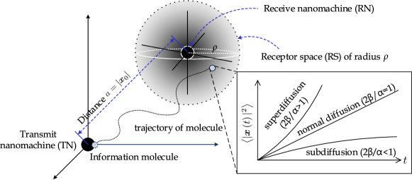
Figure 1: An illustration of a 3-D molecular communication system with anomalous diffusion.

II-B System Model

We consider an $m$-D MC system including a transmit nanomachine (TN) located at the origin which communicates with a receive nanomachine (RN) located at $\bm{x}_{0}\in\mathbbmss{R}^{m}$, $m\in\left\{1,2,3\right\}$, from TN by releasing information molecules obey an anomalous diffusion law (see Fig. 1 for illustrating the 3-D molecular communication system as an example). The transmit information modulates the number of molecules emitted by TN. We consider the burst transmission of an information sequence of finite length. Let $\mathcal{S}\triangleq\left\{s_{1},s_{2},\ldots,s_{\kappa}\right\}$ be the information sequence consisting of $\kappa$ time slots with a bit interval $T_{\mathrm{b}}$, where $s_{i}\in\left\{0,1\right\}$ denotes the $i$th transmitted bit, $1\leq i\leq\kappa$. The TN emits $N$ molecules at the beginning of a bit interval to transmit bit ‘1’ whereas no molecule is emitted for bit ‘0’ transmission.

To decode the information, the RN counts the number of molecules inside the RS of radius $\rho$ at the observation time. Note that the MC channel is assumed to be isotropic and symmetric, we will omit the vector notation of $\bm{x}_{0}$ in all following equations in the rest of this paper. To focus on the characteristics of the anomalous diffusion channel, we assume that the MC system satisfies the following assumptions: i) the number of information molecules for each symbol are controlled by the TN perfectly; ii) the clocks of the TN and RN are synchronized; iii) the information molecules are randomly and freely propagated within the anomalous diffusion medium; and iv) the RN perfectly counts the number of molecules in the RS at the observation time. In addition, to exemplify the anomalous diffusive propagation environment, throughout the remainder of this paper, we set diffusion parameters $\alpha=2$ and $\beta=1$ for normal diffusion, $\alpha=2$ and $\beta=0.5$ for subdiffusion, and $\alpha=1.8$ and $\beta=1$ for superdiffusion with $K=10^{-10}$ [m²/s], $a=5$ [$\mu$m], and $\rho=0.5$ [$\mu$m].

III Reception and Detection Processes

III-A Reception Process

For the passive receiver of interest, we assume that the probability that the information molecules are observed inside the RS is equal to the one at the RN located at the center of the RS. In addition, when the TN is sufficiently far from the RS, the precise shape is irrelevant. We also take into consideration lifetime limited molecules whose life expectancy follows an exponential distribution such that

$$h\left(\tau\right) =\lambda e^{-\lambda\tau}$$ (10)

where $\lambda$ is the degradation rate of the molecules and $\tau$ denotes the molecules’ lifetime [19, 20]. It implies that a molecule can be inside the RS at time $t$ only if its lifetime is greater than $t$, that is $\tau\in\left(t,\infty\right)$. Note that $\lambda=0$ corresponds to the no degradation case. Then, the probability that the information molecules with the degradation rate $\lambda$ stay inside the RS of volume $V_{\rho}$ at the observation time $t$, denoted by $P\left(t|V_{\rho},\lambda\right)$, is

$$P\left(t|V_{\rho},\lambda\right) =\int_{V_{\rho}}\omega\left(\bm{x},t\right)\int_{t}^{\infty}h\left(\tau\right)d\tau d\bm{x}$$ (11)

$$\approx V_{\rho}\omega\left(a,t\right)e^{-\lambda t}$$ (12)

where

$$V_{\rho} =\begin{cases}2\rho,&\text{ if $m=1$}\\ \pi\rho^{2},&\text{ if $m=2$}\\ \frac{4}{3}\pi\rho^{3},&\text{ if $m=3$}.\end{cases}$$ (13)

The expected number of observed molecules inside the RS, denoted by $\bar{N}_{\mathrm{ob}}\left(t\right)$, is given by [12, 13]

$$\bar{N}_{\mathrm{ob}}\left(t\right)=V_{\rho}N\omega\left(a,t\right)e^{-\lambda t}.$$ (14)

Since $\bar{N}_{\mathrm{ob}}\left(t\right)$ is the concave function on the interval $t>0$, $\bar{N}_{\mathrm{ob}}\left(t\right)$ obviously has a global maximum value at certain time $t$. Let $t_{\mathrm{p}}$ be the peak time at $t_{\mathrm{p}}=\mathop{\mathrm{arg\,max}}_{t}\,\bar{N}_{\mathrm{ob}}\left(t\right)$. Then, $t_{\mathrm{p}}$ can be found as

$$\left.\frac{d\bar{N}_{\mathrm{ob}}\left(t\right)}{dt}\right|_{t=t_{\mathrm{p}}}=0.$$ (15)

Theorem 1 (Peak Time in $m$-D Anomalous Diffusion)

Given the diffusion parameters $\alpha$, $\beta$, $K$, $a$, and $\lambda$, the peak time $t_{\mathrm{p}}$ is the solution of

$$H^{1,3}_{4,3}\left[{\frac{K^{\frac{1}{\beta}}t_{\mathrm{p}}}{\left(a/2\right)^{\frac{\alpha}{\beta}}}}\left|\begin{array}[]{c}{\left(0,1\right),\bigl{(}0,\tfrac{1}{\beta}\bigr{)},\bigl{(}\tfrac{2-m}{2},\tfrac{\alpha}{2\beta}\bigr{)},\bigl{(}0,\frac{\alpha}{2\beta}\bigr{)}}\\ {\bigl{(}0,\tfrac{1}{\beta}\bigr{)},\left(0,1\right),\left(1,1\right)}\end{array}\right.\right]$$ (18)

$$=\lambda t_{\mathrm{p}}H^{1,2}_{3,2}\left[{\frac{K^{\frac{1}{\beta}}t_{\mathrm{p}}}{\left(a/2\right)^{\frac{\alpha}{\beta}}}}\left|\begin{array}[]{c}{\bigl{(}0,\frac{1}{\beta}\bigr{)},\bigl{(}\frac{2-m}{2},\frac{\alpha}{2\beta}\bigr{)},\bigl{(}0,\frac{\alpha}{2\beta}\bigr{)}}\\ {\bigl{(}0,\frac{1}{\beta}\bigr{)},\bigl{(}0,1\bigr{)}}\end{array}\right.\right].$$ (21)

Proof:

It follows readily from the differential operation of Fox’s $H$-function [18, Property 4]. ∎

Specifically, we commonly set $T_{\mathrm{b}}>t_{\mathrm{p}}$ and $t_{\mathrm{p}}$ is equal to $a^{2}/\left(2mK\right)$ in normal diffusion when $\lambda=0$ [11, 12].

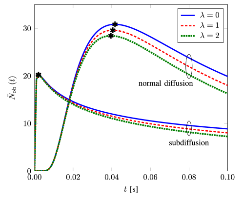
Figure 2: Expected number of molecules inside the RS $\bar{N}_{\mathrm{ob}}\left(t\right)$ as a function of $t$ in normal diffusion and subdiffusion for $\lambda=0,1,2$ when $m=3$ and $N=10^{5}$.

The expected number of molecules inside the RS $\bar{N}_{\mathrm{ob}}\left(t\right)$ is shown for normal diffusion and subdiffusion in Fig. 2 and for superdiffusion in Fig. 3 as a function of $t$ for $\lambda=0$, $1$, and $2$ when $m=3$ and $N=10^{5}$. We can see that $\bar{N}_{\mathrm{ob}}\left(t\right)$ increases over time until reaching its peak time $t_{\mathrm{p}}$, and then monotonically decreasing with time. For example, $t_{\mathrm{p}}$ for normal diffusion, subdiffusion, and superdiffusion are equal to $0.0417$, $0.0021$ and $0.6287$ when $\lambda=0$. Since the subdiffusion information molecules are most rapidly propagated in space while the superdiffusion molecules are spreading slowly in space, the largest $t_{\mathrm{p}}$ is observed in superdiffusion while subdiffusion has the smallest $t_{\mathrm{p}}$. Note that with sufficiently large $a$ and $K$, superdiffusion is expected to have the largest $t_{\mathrm{p}}$ [6]. Moreover, we can observe that $\bar{N}_{\mathrm{ob}}\left(t\right)$ decreases with the degradation rate $\lambda$, for example, $t_{\mathrm{p}}$ for $\lambda=1$ and $2$ in Fig. 3 are 0.4824 and 0.4099, respectively.

III-B Detection Process

Let $t_{\mathrm{o}}$ be the observation time that the RN counts the number of information molecules inside the RS after the beginning of the $i$th bit interval in order to decode the bit $s_{i}$, $1\leq i\leq\kappa$, $t_{\mathrm{o}}\in\left(0,T_{\mathrm{b}}\right]$. Let $\mathcal{S}_{i}\triangleq\left\{s_{1},s_{2},\ldots,s_{i-1}\right\}$ be an ISI sequence of the $i$th bit transmission consisting of all previous bit transmission $s_{j}$, $1\leq j<i$. The probability that the molecule emitted at the $j$th bit transmission inside the RS at $t_{\mathrm{o}}$ is equal to $P\left(\left(i-j\right)T_{\mathrm{b}}+t_{\mathrm{o}}|V_{\rho},\lambda\right)$. Then, the total number of molecules counted by the RN for the detection of the $i$th bit transmission, denoted by $y_{i}$, is distributed as

$$y_{i} \sim\sum_{j=1}^{i}s_{j}\mathrm{Binom}\left({N},{P\left(\left(i-j\right)T_{\mathrm{b}}+t_{\mathrm{o}}|V_{\rho},\lambda\right)}\right)$$ (22)

where $\mathrm{Binom}\left({x},{y}\right)$ denotes the binomial distribution with mean $xy$ and variance $xy\left(1-y\right)$. Since the sum of binomial distribution is mathematically not tractable, it can be alternatively approximated by either the Gaussian distribution or Poisson distribution. It has been shown that the Poisson approximation was indistinguishable from the binomial distribution, whereas a notable loss in accuracy was seen in the Gaussian approximation [12]. Hence, we consider a Poisson approximation for the sum of binomial random variables. Then, we have

$$y_{i}\sim\mathrm{Pois}\Biggl{(}\sum_{j=1}^{i}s_{j}NP\left(\left(i-j\right)T_{\mathrm{b}}+t_{\mathrm{o}}|V_{\rho},\lambda\right)\Biggr{)}$$ (23)

where $\mathrm{Poisson}\left(x\right)$ denotes the Poisson distribution with the mean $x$. The $i$th information bit $s_{i}$ can be decoded by using the following detection rule:

$$\hat{s}_{i} =\begin{cases}1,\quad\text{if $y_{i}\geq\gamma_{i}$}\\ 0,\quad\text{if $y_{i}<\gamma_{i}$}\end{cases}$$ (24)

where $\gamma_{i}>0$ is the decision threshold for the $i$th transmitted bit.

IV Error Probability

IV-A Single-Bit Interval Transmission

We first consider a SBIT with $\kappa=1$. In this case, the total number of molecules counted by the RN at $t_{\mathrm{o}}$ for the detection of the $i$th bit transmission is distributed as

$$y_{i} \sim\mathrm{Binom}\left({N},{P\left(t_{\mathrm{o}}|V_{\rho},\lambda\right)}\right).$$ (25)

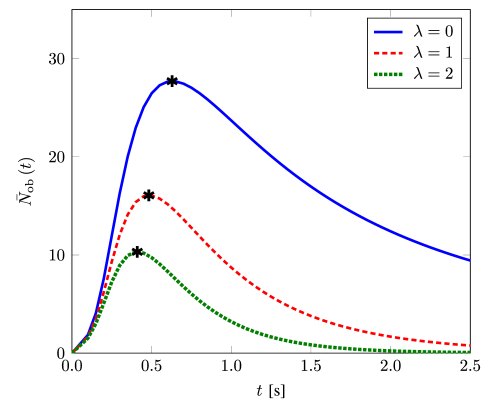
Figure 3: Expected number of molecules inside the RS $\bar{N}_{\mathrm{ob}}\left(t\right)$ as a function of $t$ in superdiffusion for $\lambda=0,1,2$ when $m=3$ and $N=10^{5}$.

Theorem 2 (BER of SBIT)

For equally-likely information bits $s_{i}$, the BER $P_{\mathrm{b}}$ of SBIT with the decision threshold $\gamma_{i}$ is given by

$$P_{\mathrm{b}} =\frac{1}{2}I_{q}\left(N-\gamma_{i}+1,\gamma_{i}\right)$$ (26)

where $q=1-P\left(t_{\mathrm{o}}|V_{\rho},\lambda\right)$, and $I_{x}\left(\cdot,\cdot\right)$ is the regularized incomplete beta function [21, eq. (8.392)].

Proof:

Since no molecule is emitted when bit ‘0’ is transmitted, with $\gamma_{i}>0$, $P_{e}$ is given by

$$P_{\mathrm{b}} =\frac{1}{2}\operatorname{\mathds{P}}\left\{{\hat{s}=0|s=1}\right\}=\frac{1}{2}\operatorname{\mathds{P}}\left\{{y_{i}<\gamma_{i}|s=1}\right\}.$$ (27)

From which and the cumulative distribution function (CDF) expression of binomial distribution, we arrive at the desired result. ∎

Remark 1 (Optimal Observation Time)

Let $t^{\star}_{\mathrm{o}}$ be the optimal observation time in which $t^{\star}_{\mathrm{o}}=\mathop{\mathrm{arg\,min}}_{t}P_{\mathrm{b}}$. Then, $t^{\star}_{\mathrm{o}}$ is the solution of

$$\left.\frac{d\left(1-V_{\rho}\omega\left(a,t\right)e^{-\lambda t}\right)}{dt}\right|_{t=t^{\star}_{\mathrm{o}}}=0.$$ (28)

Then, it is readily shown that $t^{\star}_{\mathrm{o}}=t_{\mathrm{p}}$.

Remark 2 (Optimal Decision Threshold)

Since $P_{\mathrm{b}}$ is the CDF of binomial distribution, the optimal decision threshold that minimizes $P_{\mathrm{b}}$ is obviously equal to $1$. With $\gamma_{i}=1$, $P_{\mathrm{b}}$ in (26) reduces to $P_{\mathrm{b}}=\frac{1}{2}\left(1-P\left(t_{\mathrm{o}}|V_{\rho},\lambda\right)\right)^{N}$.

Remark 3 (Transmit Diversity Gain)

Let

$$\xi\triangleq\lim_{N\rightarrow\infty}\frac{-\log P_{\mathrm{b}}}{N}$$ (29)

be the transmit diversity gain of the BER $P_{\mathrm{b}}$. Then by applying L’Hôpitals’s rule for $0<p<1$, and with the fact that

$$\lim_{x\rightarrow\infty}\frac{-\log I_{p}\left({x},{y}\right)}{x}=-\log p$$

we have

$$\xi =\log\left(\frac{1}{1-P\left(t_{\mathrm{o}}|V_{\rho},\lambda\right)}\right).$$ (30)

This reveals that the reliability of the MC system can be enhanced from the consumption of more molecular resources, which is synonymous with the transmit diversity gain in multi-antenna wireless communication systems. It is also noteworthy that $\xi$ is not a function of the detection threshold.

IV-B Multi-Bit Interval Transmission

In a MBIT with $\kappa>1$, we assume that the RN can keep the transmitted sequence history $\mathcal{S}_{i}$ (the memory detector) [9].

Theorem 3 (Conditional BER of MBIT)

Let

$$\mu^{\left(k\right)}_{i} =\sum_{j=1}^{i-1+k}s_{j}NP\left(\left(i-j\right)T_{\mathrm{b}}+t_{\mathrm{o}}|V_{\rho}\lambda\right)$$ (31)

be the average of $y_{i}$ when the information bit $s_{i}=k$, $k\in\left\{0,1\right\}$. For equally-likely information bits $s_{i}$, the conditional BER of the $i$th bit in the burst transmission given $\mathcal{S}_{i}$, denoted by $P_{\left.\mathrm{b}\right|{\mathcal{S}_{i}}}$, with the decision threshold $\gamma_{i}$ is given by

$$P_{\left.\mathrm{b}\right|{\mathcal{S}_{i}}} =\frac{1}{2}\left(1-\frac{\sum_{k=0}^{1}\left(-1\right)^{k}\Gamma\left(\lfloor\gamma_{i}\rfloor,\mu^{\left(k\right)}_{i}\right)}{\lfloor\gamma_{i}-1\rfloor!}\right)$$ (32)

where $\Gamma\left(\mu,\sigma\right)$ is the upper incomplete Gamma function [21, eq. (8.350)] and $\lfloor x\rfloor$ denotes the floor function.

Proof:

For equiprobable bits ‘0’ and ‘1’, we have

$$P_{\left.\mathrm{b}\right|{\mathcal{S}_{i}}} =\frac{1}{2}\left(\operatorname{\mathds{P}}\left\{{y_{i}\geq\gamma_{i}|s_{i}=0,\mathcal{S}_{i}}\right\}+\operatorname{\mathds{P}}\left\{{y_{i}<\gamma_{i}|s_{i}=1,\mathcal{S}_{i}}\right\}\right).$$

From which and the CDF expression of Poisson distribution, we obtain the desired result. ∎

Note that it is needed to average on all possible ISI sequences with their probabilities of occurrence to calculate the average BER. We only consider $\mathcal{S}_{i}=\mathbf{1}_{i-1}$ in the following section for the most serious ISI performance analysis where $\mathbf{1}_{n}$ denotes an all-one sequence of $n$ elements.

Remark 4

For the memory detector, the optimal $\gamma_{i}$ can be found using the maximum likelihood such that [9]

$$\gamma_{i}=\frac{\mu^{\left(0\right)}_{i}-\mu^{\left(1\right)}_{i}}{\log{\mu^{\left(0\right)}_{i}}-\log{\mu^{\left(1\right)}_{i}}}.$$ (33)

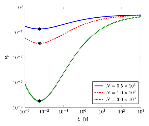
Figure 4: BER $P_{\mathrm{b}}$ of SBIT as a function of $t_{\mathrm{o}}$ in subdiffusion when $m=3$.

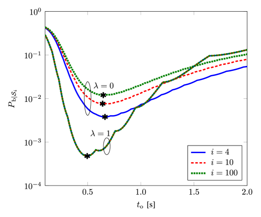
Figure 5: BER $P_{\left.\mathrm{b}\right|{\mathcal{S}_{i}}}$ of $s_{i}$ in MBIT as a function of $t_{\mathrm{o}}$ in superdiffusion when $m=3$.

IV-C Numerical Examples

Fig. 4 shows the BER $P_{\mathrm{b}}$ of SBIT as a function of observation time $t_{\mathrm{o}}$ in subdiffusion for i) $N=0.5\times 10^{3}$, ii) $1.0\times 10^{3}$, and iii) $3.0\times 10^{3}$ when $\lambda=0$, $\gamma_{i}=1$, and $m=2$. We observe that the BER decreases as the number of emitted molecules $N$ increases. In addition, the minimum $P_{\mathrm{b}}$ is achieved at the optimal observation time $t_{\mathrm{o}}=t_{\mathrm{p}}=0.0055$ [s] as described in Remark 1 and Remark 2. Fig 5 shows the BER $P_{\left.\mathrm{b}\right|{\mathcal{S}_{i}}}$ of $s_{i}$ in MBIT with $\mathcal{S}_{i}=\mathbf{1}_{i-1}$ as a function of $t_{\mathrm{o}}$ in superdiffusion for i) $i=4$, ii) $i=10$, and iii) $i=100$ with $\lambda=0$ and $\lambda=1$ when $T_{\mathrm{b}}=2$, $m=3$, and $N=10^{5}$. The decision threshold $\gamma_{i}$ is found using (33). We can see that the observation time that minimizes $P_{\left.\mathrm{b}\right|{\mathcal{S}_{i}}}$ is not equal to the one given in Remark 1 due to the ISI effect. Indeed, the large size of the interference sequence gives BER performance degradation while the lifetime limited interfering molecules reduces the ISI effect on the BER performance. It can be expected that if $t_{\mathrm{o}}$ is near to $T_{\mathrm{b}}$, though the less ISI is cumulated, but the number of observed information molecules decreases as well. Therefore, it leads to a higher BER in general. Furthermore, it is seen that the BER converges for $i$ $\geq 4$ where $\lambda=1$. However, the performance consistently degrades as $i$ increases when $\lambda=0.$ It means that a reliable continuous transmission can be achieved only with lifetime limited molecules.

The BER $P_{\left.\mathrm{b}\right|{\mathcal{S}_{i}}}$ of $s_{i}$ in SBIT and MBIT ($i=4$ with $\mathcal{S}_{i}=\mathbf{1}_{i-1}$) as a function of $N$ is shown in Fig. 6 for i) normal diffusion, ii) subdiffusion, and iii) superdiffusion when $\lambda=0$, $t_{\mathrm{o}}=t_{\mathrm{p}}$, $m=2$. For SBIT, we set $\gamma_{i}=1$, while $\gamma_{i}$ can be found using (33) for MBIT. It can obviously be seen that the BER decreases as $N$ increases. In the case of SBIT, the transmit diversity gain $\xi$ are equal to $0.00160$, $0.00115$, and $0.00148$ for normal diffusion, subdiffusion, and superdiffusion, respectively, as stated in Remark 3. It reveals that the BER in normal diffusion outperforms that in other diffusion scenarios for the large $N$ in this example. The transmit diversity gain for MBIT, which can be evaluated numerically, is tabulated in Table I for $i=2,3,4$ with $\mathcal{S}_{i}=\mathbf{1}_{i-1}$. It is shown that the ISI decreases transmit diversity gain significantly, as expected.

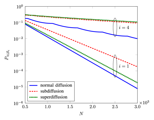
Figure 6: BER $P_{\left.\mathrm{b}\right|{\mathcal{S}_{i}}}$ of $s_{i}$ in SBIT and MBIT as a function of $N$ when $m=2$.

TABLE I: Transmit Diversity Gain $\xi$

	$i$
Diffusion scenario	$1$	$2$	$3$	$4$
Normal diffusion	$0.00160$	$0.00057$	$0.00051$	$0.00050$
Subdiffusion	$0.00115$	$0.00030$	$0.00023$	$0.00019$
Superdiffusion	$0.00148$	$0.00026$	$0.00021$	$0.00018$

The BER $P_{\left.\mathrm{b}\right|{\mathcal{S}_{i}}}$ of $s_{i}$ in MBIT with $\mathcal{S}_{i}=\mathbf{1}_{i-1}$ is shown in Fig. 7 as a function of $\gamma_{i}$ for i) $\lambda=0$ and ii) $\lambda=1$ in superdiffusion when $T_{\mathrm{b}}=2$, $t_{\mathrm{o}}=t_{\mathrm{p}}$, $m=3$, and $N=10^{5}$. With the observation time $t_{\mathrm{o}}=t_{\mathrm{p}}$, the decision threshold that minimizes $P_{\left.\mathrm{b}\right|{\mathcal{S}_{i}}}$ is varying with respect to the number of expected interfering molecules. For example, with $\lambda=0$, $\gamma_{i}$ is equal to $27$ for $i=4$, and $\gamma_{i}$ is equal to $33$ for $i=10$. It can be found the optimal decision threshold is numerically equal to the ceiling of $\gamma_{i}$ given in Remark 4. We also find it noteworthy that the ISI effects can be controlled simply by taking the lifetime limited molecules into consideration.

V Conclusion

In this paper, we studied the MC system in anomalous diffusion channels with the RS at the receiver side. The peak time of the expected number of observed molecules inside the RS has been presented. In addition, we analyzed the performance of the MC system in terms of BER. It has been shown that the peak time is the optimal observation time that minimizes the BER in the SBIT. In the MBIT, the BER has been derived with a given ISI sequence. The corresponding observation time and decision threshold that are minimizing BER can be found numerically. It has been shown that introducing lifetime limited molecules is an effective approach for the alleviation of the ISI in the MBIT. A more realistic diffusion environment for various applications of MC systems, i.e., anomalous diffusion in an inhomogeneous medium, will be developed in future studies.

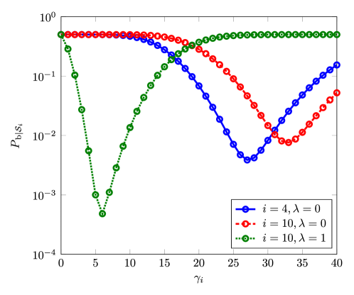
Figure 7: BER $P_{\left.\mathrm{b}\right|{\mathcal{S}_{i}}}$ of $s_{i}$ in MBIT as a function of $\gamma_{i}$ in superdiffusion when $m=3$.

References

- [1] T. Nakano, A. W. Eckford, and T. Haraguchi, Molecular Communication, 1st ed. New York: Cambridge University Press, 2013.
- [2] M. Weiss, M. Elsner, F. Kartberg, and T. Nilsson, “Anomalous subdiffusion is a measure for cytoplasmic crowding in living cells,” Biophys. J., vol. 87, pp. 3518–3524, Nov. 2004.
- [3] F. Matthäus, M. Jagodič, and J. Dobnikar, “E. coli superdiffusion and chemotaxis–search strategy, precision, and motility,” Biophys. J., vol. 97, no. 4, pp. 946–957, Aug. 2009.
- [4] F. A. Oliveira, R. M. S. Ferreira, L. C. Lapas, and M. H. Vainstein, “Anomalous diffusion: A basic mechanism for the evolution of inhomogeneous systems,” Frontiers in Physics., vol. 17, no. 19, pp. 1–17, Feb. 2019.
- [5] T. N. Cao, D. P. Trinh, Y. Jeong, and H. Shin, “Anomalous diffusion in molecular communication,” IEEE Commun. Lett., vol. 19, no. 10, pp. 1674–1677, Oct. 2015.
- [6] D. P. Trinh, Y. Jeong, and H. Shin, “Connectivity in molecular communication with random time constraints,” IEEE Access, vol. 7, pp. 113 121–113 130, Aug. 2019.
- [7] D. P. Trinh, Y. Jeong, H. Shin, and M. Z. Win, “Molecular communication with anomalous diffusion in stochastic nanonetworks,” IEEE Trans. Commun., vol. 67, no. 12, pp. 8378–8393, Dec. 2019.
- [8] M. U. Mahfuz, D. Makrakis, and H. T. Mouftah, “Concentration-encoded subdiffusive molecular communication: Theory, channel characteristics, and optimum signal detection,” IEEE Trans. NanoBiosci., vol. 15, no. 6, pp. 533–548, Sep. 2016.
- [9] S. Huang, L. Lin, J. Xu, W. Guo, and H. Y, “Molecular communication via subdiffusion with a spherical absorbing receiver,” IEEE Wireless Commun. Lett., vol. 9, no. 10, pp. 1682–1686, Oct. 2020.
- [10] D. P. Trinh, Y. Jeong, H. Shin, and M. Z. Win, “-diffusion for molecular communication,” IEEE Trans. Commun., vol. 68, no. 7, pp. 4293–4310, Jul. 2020.
- [11] L.-S. Meng, P.-C. Yeh, K.-C. Chen, and I. F. Akyildiz, “On receiver design for diffusion-based molecular communication,” IEEE Trans. Signal Process., vol. 62, no. 22, pp. 6032–6044, Nov. 2014.
- [12] A. Noel, K. C. Cheung, and R. Schober, “Improving receiver performance of diffusive molecular communication with enzymes,” IEEE Trans. NanoBiosci., vol. 13, no. 1, pp. 31–43, Mar. 2014.
- [13] Y. Deng, A. Noel, W. Guo, A. Nallanathan, and M. Elkashlan, “Analyzing large scale multiuser molecular communication via 3-D stochastic geometry,” IEEE Trans. Mol. Biol. Multi-Scale Commun., vol. 3, no. 2, pp. 118–133, Jun. 2017.
- [14] V. Honary, M. Nitz, B. J. Wysocki, and T. A. Wysocki, “Modeling -d diffusion using queuing networks,” BioSystems, vol. 179, Dec. 2019.
- [15] V. Honary and T. A. Wysocki, “Molecular communication system with non-absorbing receiver,” Nano Commun. Netw., vol. 28, Jun. 2021.
- [16] V. V. Uchaikin, “Anomalous diffusion and fractional stable distribution,” J. Exp. Theor. Phys., vol. 97, no. 4, pp. 810–825, 2003.
- [17] V. M. Zolotarev, V. V. Uchaikin, and V. V. Saenko, “Superdiffusion and stable laws,” J. Exp. Theor. Phys., vol. 88, no. 4, p. 780–787, Apr. 1999.
- [18] Y. Jeong, H. Shin, and M. Z. Win, “-transforms for wireless communication,” IEEE Trans. Inf. Theory, vol. 61, no. 7, pp. 3773–3809, Jul. 2015.
- [19] A. Singhal, R. K. Mallik, and B. Lall, “Performance analysis of amplitude modulation schemes for diffusion-based molecular communication,” IEEE Trans. Wireless Commun., vol. 14, no. 10, pp. 5681–5691, Oct. 2015.
- [20] W. Guo, T. Asyhari, N. Farsad, H. B. Yilmaz, B. Li, A. Eckford, and C.-B. Chae, “Molecular communications: Channel model and physical layer techniques,” IEEE Trans. Wireless Commun., vol. 23, no. 4, pp. 120–127, Aug. 2016.
- [21] I. S. Gradshteyn and I. M. Ryzhik, Table of Integrals, Series, and Products, 7th ed. San Diego, CA: Academic, 2007.