Asymptotic normality of robust $M$-estimators with convex penalty

Abstract

This paper develops asymptotic normality results for individual coordinates of robust M-estimators with convex penalty in high-dimensions, where the dimension $p$ is at most of the same order as the sample size $n$, i.e, $p/n\leq\gamma$ for some fixed constant $\gamma>0$. The asymptotic normality requires a bias correction and holds for most coordinates of the M-estimator for a large class of loss functions including the Huber loss and its smoothed versions regularized with a strongly convex penalty.

The asymptotic variance that characterizes the width of the resulting confidence intervals is estimated with data-driven quantities. This estimate of the variance adapts automatically to low ($p/n\to 0)$ or high ($p/n\leq\gamma$) dimensions and does not involve the proximal operators seen in previous works on asymptotic normality of M-estimators. For the Huber loss, the estimated variance has a simple expression involving an effective degrees-of-freedom as well as an effective sample size. The case of the Huber loss with Elastic-Net penalty is studied in details and a simulation study confirms the theoretical findings. The asymptotic normality results follow from Stein formulae for high-dimensional random vectors on the sphere developed in the paper which are of independent interest.

Keywords:Robust estimation, M-estimator, Asymptotic normality, Confidence Intervals, High-dimensional statistics, Bias-correction, Stein’s formula.

1 Introduction

1.1 Robust inference

In his seminal paper on robustness, Huber [20] introduced $M$-estimators for an unknown location parameter $\mu\in\mathbb{R}$ from observations $Y_{i}=\mu+\varepsilon_{i}$, $i=1,\ldots,n$, where $\varepsilon_{i}$ are iid noise random variables distributed as a mixture $F=(1-\epsilon)N(0,1)+\epsilon H$ with $H$ being the distribution of the contaminated samples, possibly chosen by an adversary. Given a differentiable loss function $\rho:\mathbb{R}\to\mathbb{R}$ and its derivative $\psi=\rho^{\prime}$, Huber defined $M$-estimators as minimizers $\hat{\mu}=\operatorname*{argmin}_{b\in\mathbb{R}}\sum_{i=1}^{n}\rho(Y_{i}-b)$, or equivalently as solutions to $\sum_{i=1}^{n}\psi(Y_{i}-b)=0$. Huber [20] went on to prove consistency and asymptotic normality of such $M$-estimators, obtaining among other results that if $\rho$ is convex and $\psi$ is absolutely continuous, then under mild assumptions on $F$, the convergence $\hat{\mu}\to\mu$ in probability holds as well as the asymptotic normality

$$n^{1/2}(\hat{\mu}-\mu)\to^{d}{N\bigl{(}0,\mathbb{E}[\psi^{2}(\varepsilon_{1})]\big{/}\mathbb{E}[\psi^{\prime}(\varepsilon_{1})]^{2}\bigr{)}.}$$

Huber’s $M$-estimators were extended to regression models, where a design matrix $\bm{X}\in\mathbb{R}^{n\times p}$ is observed together with responses $y_{i}=\bm{x}_{i}^{\top}{\bm{\beta}}+\varepsilon_{i}$ where $\bm{x}_{1},...,\bm{x}_{n}$ are the rows of $\bm{X}$ and $\varepsilon_{1},...,\varepsilon_{n}$ are possibly contaminated noise random variables as in the previous paragraph. For fixed or slowly growing dimension $p$ as $n\to+\infty$, consistency and asymptotic normality of $M$-estimators of the form $\hat{{\bm{\beta}}}=\operatorname*{argmin}_{\bm{b}\in\mathbb{R}^{p}}\sum_{i=1}^{n}\rho(y_{i}-\bm{x}_{i}^{\top}\bm{b})$ were obtained, see [21, Section 7] or [27] among others. Explicitly, if $\bm{e}_{j}\in\mathbb{R}^{p}$ is a canonical basis vector and one is interested in the asymptotic normality of $\hat{\beta}_{j}-\beta_{j}$ for the purpose of confidence intervals, [27] shows that

$$\bigl{(}\bm{e}_{j}^{\top}(\bm{X}^{\top}\bm{X}/n)^{-1}\bm{e}_{j}\bigr{)}^{-1/2}~{}\sqrt{n}(\hat{\beta}_{j}-\beta_{j})~{}\to^{d}~{}N\Bigl{(}0,\frac{\mathbb{E}[\psi^{2}(\varepsilon_{1})]}{\mathbb{E}[\psi^{\prime}(\varepsilon_{1})]^{2}}\Bigr{)}$$ (1.1)

if $(p\log n)^{3/2}/n\to 0$ and under mild assumptions on $\bm{X}$. As in the location parameter problem of the previous paragraph, the asymptotic variance is characterized by the ratio $\mathbb{E}[\psi^{2}(\varepsilon_{1})]/\mathbb{E}[\psi^{\prime}(\varepsilon_{1})]^{2}$.

The last decade has seen striking developments of similar asymptotic normality results in high-dimensions, where $p/n\to\gamma$ for some constant $\gamma<1$, cf. [17, 3, 25, 15, 16]. In terms of asymptotic normality, these works show that if $\bm{X}$ has iid $N(0,\bm{\Sigma})$ rows, the unregularized $M$-estimator $\hat{{\bm{\beta}}}=\operatorname*{argmin}_{\bm{b}\in\mathbb{R}^{p}}\sum_{i=1}^{n}\rho(y_{i}-\bm{x}_{i}^{\top}\bm{b})$ satisfies asymptotic normality of the form

$$(\bm{e}_{j}^{\top}\bm{\Sigma}^{-1}\bm{e}_{j})^{-1/2}~{}\sqrt{p}(\hat{\beta}_{j}-\beta_{j})\to^{d}N(0,r^{2})$$ (1.2)

where $r>0$ is a deterministic constant that captures the high-dimensionality of the problem [17, Lemma 1]. The constant $r>0$ is determined by solving a system of nonlinear equations with two unknowns: In the unregularized setting, [17, S2] describes this system of nonlinear equations with unknowns $(r,c)$ as

$$\left\{\begin{aligned} \mathbb{E}\bigl{[}1-[\text{prox}_{c}(\rho)]^{\prime}(\varepsilon_{1}+rZ)\bigr{]}&=\gamma,\\ \mathbb{E}\bigl{[}\bigl{(}\varepsilon_{1}+rZ-[\text{prox}_{c}(\rho)](\varepsilon_{1}+rZ)\bigr{)}^{2}\bigr{]}&=\gamma r^{2}\end{aligned}\right.\qquad\text{ as }~{}p/n\to\gamma,$$ (1.3)

where $Z\sim N(0,1)$ is independent of $\varepsilon_{1}$, and $\operatorname*{prox}_{c}(\rho)(t)=\operatorname*{argmin}_{u\in\mathbb{R}}\rho(u)+(t-u)^{2}/(2c)$ denotes the proximal operator of the convex function $t\to c\rho(t)$ with derivative $[\text{prox}_{c}(\rho)]^{\prime}(t)$. The optimality conditions

$$c^{-1}(t-[\text{prox}_{c}(\rho)](t))=\psi([\text{prox}_{c}(\rho)](t))$$

of the proximal minimization problem leads to the expressions $c^{-2}\gamma r^{2}=\mathbb{E}[\psi([\text{prox}_{c}(\rho)](\varepsilon_{1}+rZ))^{2}]$ and $c^{-1}\gamma=\mathbb{E}[\frac{d}{dt}\psi([\text{prox}_{c}(\rho)](t))|_{t=\varepsilon_{1}+rZ}]$ for the solutions $(r,c)$ to the above system. Hence (1.2) can be rewritten as

$$(\bm{e}_{j}^{\top}\bm{\Sigma}^{-1}\bm{e}_{j})^{-1/2}\sqrt{n}(\hat{\beta}_{j}-\beta_{j})~{}\to^{d}~{}N\Bigl{(}0,\frac{\mathbb{E}[\psi([\text{prox}_{c}(\rho)](\varepsilon_{1}+rZ))^{2}]}{\mathbb{E}[\frac{d}{dt}\psi([\text{prox}_{c}(\rho)](t))|_{t=\varepsilon_{1}+rZ}]^{2}}\Bigr{)},$$ (1.4)

see, e.g., [15, Theorem 4.1 and Corollary 4.6]. These results embody that when $p$ and $n$ are of the same order, the asymptotic variance in (1.1) must be modified to account for the high-dimensionality of the problem by (a) replacing $\psi$ in the numerator and $\psi^{\prime}$ in the denominator by their compositions with the proximal operator $\text{prox}_{c}(\rho)$, and (b) adding the extra Gaussian term $rZ$ to the initial noise $\varepsilon_{1}$. The distribution of $\varepsilon_{1}+rZ$ is sometimes referred to as the effective noise. The Gaussian assumption can be relaxed and some of the above results are still valid if $\bm{X}$ has iid centered entries with variance one [25, 16]. Despite the subtle introduction of the proximal operator and the constants $(r,c)$, it is remarkable that the informal ratio $\frac{\text{average}[\psi^{2}]}{\text{average}[(d/dt)\psi]^{2}}$ unifies the results (1.1) and (1.4) in both low and high-dimensions.

All results of the previous section are applicable when $p/n\to\gamma$ with $\gamma<1$. For $\gamma>1$ regularization is required to ensure the uniqueness of $\hat{{\bm{\beta}}}$, for instance through an additive penalty which leads to regularized $M$-estimators of the form

$$\hat{{\bm{\beta}}}=\operatorname*{argmin}_{\bm{b}\in\mathbb{R}^{p}}\frac{1}{n}\sum_{i=1}^{n}\rho(y_{i}-\bm{x}_{i}^{\top}\bm{b})+g(\bm{b})$$ (1.5)

for some convex penalty function $g:\mathbb{R}^{p}\to\mathbb{R}$. The case of Ridge regularization with $g(\bm{b})=\tau\|\bm{b}\|_{2}^{2}/2$ for some constant $\tau>0$ is treated in [25, 16]. In this case, the two solutions $(r,c)$ of a system of two nonlinear equations similar to (1.3) characterize the error $\|\hat{{\bm{\beta}}}-{\bm{\beta}}\|_{2}$, asymptotic normality and asymptotic variance of $\sqrt{n}((1+a)\hat{\beta}_{j}-\beta_{j})$ where $a$ is a constant capturing the bias induced by regularization [16, Proposition 3.30] and $a$ is a function of $(\gamma,r,c)$. [29] characterize the error $\|\hat{{\bm{\beta}}}-{\bm{\beta}}\|_{2}$ for a large class of $(\rho,g)$ pairs using a technique known as the Convex Gordon Min-Max theorem pioneered by [28], and the recent paper [19] on Approximate Message Passing focused on $g(\bm{b})=\lambda\|\bm{b}\|_{1}$ and $\rho$ either the Huber loss or the absolute value. Little is known, however, on asymptotic normality of the regularized estimators (1.5) for penalty functions different from the square norm $\bm{b}\mapsto\tau\|\bm{b}\|_{2}^{2}$. The theories developed in [29, 19] do not readily provide asymptotic normality results and regularized $M$-estimators of the form (1.5) lack confidence interval capabilities. One goal of the present paper is to fill this gap.

A separate line of research develops asymptotic normality results and confidence intervals for regularized least-squares estimators of the form

$$\hat{{\bm{\beta}}}=\operatorname*{argmin}_{\bm{b}\in\mathbb{R}^{p}}\frac{1}{2n}\sum_{i=1}^{n}(y_{i}-\bm{x}_{i}^{\top}\bm{b})^{2}+g(\bm{b})=\operatorname*{argmin}_{\bm{b}\in\mathbb{R}^{p}}\|\bm{y}-\bm{X}\bm{b}\|_{2}^{2}/(2n)+g(\bm{b})$$ (1.6)

where $\bm{X}$ has rows $\bm{x}_{1},...,\bm{x}_{n}$. Early results studied the Lasso with $g(\bm{b})=\lambda\|\bm{b}\|_{1}$ [32, 22, 30] under a sparsity condition $s\log(p)=o(\sqrt{n})$ where $s=\|{\bm{\beta}}\|_{0}$, or Ridge regression [11]. For the Lasso the sparsity condition was later improved to $s\log^{2}(p)/n\to 0$ [24], to $s\log(p/s)/n\to 0$ [7] and $p/n\to\gamma\in(0,\infty)$ with $s\lesssim n/\log(p/s)$ ([23, 26] for isotropic Gaussian design and [13] [6, Theorem 3.2] for non-isotropic Gaussian design). For penalty functions beyond the Lasso and Ridge regularization, [12, Proposition 4.3(iii)] provides asymptotic normality on average over the coordinates for permutation invariant penalty function $g$ in (1.6), and [6, Theorem 3.1] proves asymptotic normality for individual coordinates of (1.6) under a strong convexity assumption. A high-level message of these works is that one must de-bias the regularized estimator (1.6) in order to obtain asymptotic normality at the $\sqrt{n}$-adjusted rate and construct confidence intervals. In the $p/n\to\gamma$ regime that is the focus of the present paper, this bias correction takes the following form. Under a strong convexity assumption and for $\bm{X}$ with iid $N(\mathbf{0}_{p},\bm{\Sigma})$ rows, [6] proves that for most coordinates $j=1,...,p$,

$$\frac{(n-\hat{\mathsf{df}})(\hat{\beta}_{j}-\beta_{j})+\bm{e}_{j}^{\top}\bm{\Sigma}^{-1}\bm{X}^{\top}(\bm{y}-\bm{X}\hat{{\bm{\beta}}})}{\|\bm{y}-\bm{X}\hat{{\bm{\beta}}}\|_{2}}\Omega_{jj}^{-1/2}\to^{d}N(0,1)$$ (1.7)

where $\Omega_{jj}=\bm{e}_{j}^{\top}\bm{\Sigma}^{-1}\bm{e}_{j}$ and $\hat{\mathsf{df}}$ is the effective degrees of freedom of $\hat{{\bm{\beta}}}$ defined as the Jacobian of the map $\bm{y}\mapsto\bm{X}\hat{{\bm{\beta}}}$ for fixed $\bm{X}$. For $\bm{\Sigma}=\bm{I}_{p}$ and consequently $\Omega_{jj}=1$, a similar bias correction proportional to $\bm{e}_{j}^{\top}\bm{X}^{\top}(\bm{y}-\bm{X}\hat{{\bm{\beta}}})$ is visible in the asymptotic normality result [12, Proposition 4.3(iii)], although there the coefficients $(n-\hat{\mathsf{df}})$ and $\|\bm{y}-\bm{X}\hat{{\bm{\beta}}}\|_{2}$ in (1.7) are replaced with deterministic scalar counterparts obtained by solving a system of nonlinear equations of a similar nature as (1.3). Another goal of the present paper is to equip robust $M$-estimators (1.5), with $\rho$ different than the squared loss, with de-biasing and asymptotic normality results similar to the previous display, allowing for general robust loss functions $\rho$ coupled with general convex penalty functions $g$.

1.2 Contributions

Our contributions are the following.

1. We provide de-biasing and asymptotic normality results for robust $M$-estimators with convex penalty functions when $p$ and $n$ are of the same order. This leads to confidence intervals for the $j$-th coordinate $\beta_{j}$ of the unknown coefficient vector ${\bm{\beta}}$. Asymptotic normality holds for a large class of robust loss functions, including the Huber loss and its smoothed versions.

2. Although this bias correction required for asymptotic normality resembles the one-step estimators recommended in the theory of classical $M$-estimator to improve efficiency (e.g., [8]), a notable difference from the low-dimensional case is the requirement of a degrees-of-freedom adjustment to amplify the one-step correction. For the squared loss, this degrees-of-freedom adjustment takes the form of multiplication by $(n-\hat{\mathsf{df}})$ in (1.7); one contribution of this paper is to identify the degrees-of-freedom adjustment that leads to asymptotic normality for robust and regularized $M$-estimators, beyond the squared loss.

3. The asymptotic variance is estimated by random, data-driven quantities, as opposed to the deterministic scalars $(r,c)$ that determine the asymptotic variance for unregularized estimators in (1.4). The fact that the asymptotic variance is estimated by observable quantities makes this results more suitable for confidence intervals (case in point: computing the solution $(r,c)$ of (1.3) and the asymptotic variance in (1.4) requires the knowledge of the noise distribution subject to contamination). The asymptotic normality result takes the form

   $$\hat{V}^{-1/2}\Omega_{jj}^{-1/2}\sqrt{n}(\hat{\beta}_{j}-\beta_{j})+[\text{observable bias correction}]\approx N(0,1)$$

   where the data-driven variance estimate $\hat{V}$ again is a ratio of the form $\frac{\text{average}[\psi^{2}]}{\text{average}[(d/dt)\psi]^{2}}$ for a particular sense of average to be defined in (2.13) below. Interestingly, the expression for this average and $\hat{V}$ does not involve the proximal mapping in (1.4). This informal statement will be made precise in Section 2.4 below.

4. In order to derive these new asymptotic normality results, we develop in Appendix B new identities for random vectors uniformly distributed on the Euclidean sphere. Although the argument of the present paper for asymptotic normality is closely related to that used in [6] for the squared loss, this previous theory for the squared loss for functions of standard normal vector does not extend to robust loss functions due to the lack of strong convexity of $\rho$ for robust losses, and consequently the lack of explicit lower bounds on $\frac{1}{n}\sum_{i=1}^{n}\psi(y_{i}-\bm{x}_{i}^{\top}\hat{{\bm{\beta}}})^{2}$. Developing these new identities and the corresponding asymptotic normality results for random vectors uniformly distributed on the sphere is a crucial step to overcome the lack of global strong convexity of $\rho$ for robust losses and to obtain the asymptotic normality results of the previous bullet points. These new identities provide novel Stein formulae for random vectors on the sphere and may be used more broadly for elliptical distributions.

2 Model and main results

2.1 Model and assumptions

We consider a linear model

$$\bm{y}=\bm{X}{\bm{\beta}}+{\bm{\varepsilon}},$$ (2.1)

where $\bm{y}\in\mathbb{R}^{n}$, $\bm{X}\in\mathbb{R}^{n\times p}$ and ${\bm{\varepsilon}}\in\mathbb{R}^{n}$, with a regularized M-estimator

$$\hat{{\bm{\beta}}}=\operatorname*{argmin}_{\bm{b}\in\mathbb{R}^{p}}\frac{1}{n}\sum_{i=1}^{n}\rho(y_{i}-\bm{x}_{i}^{\top}\bm{b})+g(\bm{b}),$$ (2.2)

where $\rho:\mathbb{R}\to\mathbb{R}$ is the loss and $g:\mathbb{R}^{p}\to\mathbb{R}$ is the penalty.

Assumption A (Assumptions on the loss).

Let $\rho:\mathbb{R}\to\mathbb{R}$ be convex and continuously differentiable on $\mathbb{R}$, with derivative $\psi=\rho^{\prime}$ being $L$-Lipschitz with

$$K^{2}\leq\psi^{\prime}(x)+\psi(x)^{2}\qquad\text{ for almost every }x\in\mathbb{R}$$ (2.3)

for some positive constant $K>0$ independent of $n,p$.

Two families of robust losses that do not satisfy A are non-differentiable losses such as the least absolute deviations $\rho(x)=|x|$, and $\delta$-insensitive losses such as $\rho(x)=(|x|-\delta)_{+}^{2}$ as $\psi(x)^{2}+\psi^{\prime}(x)=0$ in a neighborhood of 0. A is verified by the Huber loss $\rho(x)=\int_{0}^{|x|}\min(1,t)dt$ with $K=1$, as well as by any smooth version of the Huber loss, for instance $\rho(x)=\sqrt{1+x^{2}}$ with $K^{2}=\frac{23}{27}\approx 0.852$. The one-sided logistic loss $\rho(x)=\log(1+e^{x})$ also satisfies A. As $\psi$ is increasing, A implies that $\rho$ is $K^{2}/2$-strongly convex in the interval $\{x\in\mathbb{R}:\psi(x)^{2}\leq K^{2}/2\}$, and conversely if $\rho$ is $\mu$-strongly convex in the interval $\{x\in\mathbb{R}:\psi(x)^{2}\leq C\}$ then A is satisfied with $K^{2}=\min(\mu,C)$.

Table 1: Left: robust loss functions satisfying A: the Huber loss $x\mapsto H(x)=\int_{0}^{|x|}\min(t,1)dt$, its smoothed versions $x\mapsto\sqrt{1+x^{2}}$ and
$x\mapsto\frac{x^{2}}{2}I\{|x|\leq 1\}+(\frac{1}{6}-\frac{|x|}{2}+x^{2}-\frac{|x|^{3}}{6})I\{|x|\in(1,2)\}+(\frac{-7}{6}+\frac{3|x|}{2})I\{(|x|\geq 2)\}.$ Right: two loss functions that do not satisfy A: the absolute deviation loss $x\mapsto|x|$ and the $1$-insensitive loss $x\mapsto H[(|x|-1)_{+}]$ where $H(\cdot)$ is the Huber loss.

Assumption B (Strongly convexity of $g$).

For some constant $\tau>0$ independent of $n,p$, the penalty $g:\mathbb{R}^{p}\to\mathbb{R}$ is $\tau$-strongly convex in the sense that $\bm{x}\mapsto g(\bm{x})-\tau\|\bm{x}\|_{2}^{2}/2$ is convex.

Some useful characterizations of strong convexity are the following. Throughout, $\partial g()$ denotes the subdifferential of $g$ at $\in\mathbb{R}^{p}$. Then $g$ is $\tau$-strongly convex if and only if

$$g()-g()\geq\bm{u}^{\top}()+(\tau/2)\|\|_{2}^{2}\quad\text{ for all }\bm{u}\in\partial g()\text{ and }\in\mathbb{R}^{p}.$$ (2.4)

Similarly $g$ is $\tau$-strongly convex if and only for any $\in\mathbb{R}^{p}$

$$(\bm{u}-\bm{v})^{\top}()\geq\tau\|\|_{2}^{2}\quad\text{ for all }\bm{u}\in\partial g(),\bm{v}\in\partial g().$$ (2.5)

Assumption C.

The rows of the design matrix $\bm{X}$ are iid $N({\bm{0}},\bm{\Sigma})$ random vectors and all the eigenvalues of $\bm{\Sigma}\in\mathbb{R}^{p\times p}$ are in $[\kappa,1/\kappa]$ for some constant $\kappa\in(0,1)$ independent of $n,p$. The noise ${\bm{\varepsilon}}$ is independent of $\bm{X}$ and admits a density with respect to the Lebesgue measure.

Assumption D.

$p/n\leq\gamma$ for some constant $\gamma>0$ independent of $n,p$.

2.2 Notation

Throughout the paper, we use the notation

$$\bm{\psi}=(\psi(y_{i}-\bm{x}_{i}^{\top}\hat{{\bm{\beta}}}))_{i\in[n]},\qquad\bm{\psi}^{\prime}=(\psi^{\prime}(y_{i}-\bm{x}_{i}^{\top}\hat{{\bm{\beta}}}))_{i\in[n]},\qquad\bm{h}=\hat{{\bm{\beta}}}-{\bm{\beta}}.$$ (2.6)

For each $j\in[p]$, let $\bm{e}_{j}$ denote the $j$-th vector in the standard basis of $\mathbb{R}^{p}$, and let

$$\Omega_{jj}=\bm{e}_{j}^{\top}\bm{\Sigma}^{-1}\bm{e}_{j},\qquad\bm{z}_{j}=\bm{X}\bm{\Sigma}^{-1}\Omega_{jj}^{-1}\bm{e}_{j},\qquad\bm{Q}_{j}=\bm{I}_{p}-\bm{\Sigma}^{-1}\Omega_{jj}^{-1}\bm{e}_{j}\bm{e}_{j}^{\top}.$$ (2.7)

We remark that the above definition implies the following properties:

• $\bm{X}=\bm{X}\bm{Q}_{j}+\bm{z}_{j}\bm{e}_{j}^{\top}$ and $\bm{X}{\bm{\beta}}=\bm{X}\bm{Q}_{j}{\bm{\beta}}+\bm{z}_{j}\beta_{j}.$

• $\bm{z}_{j}\sim N({\bm{0}},\Omega_{jj}^{-1}\bm{I}_{n})$ is independent of $\bm{X}\bm{Q}_{j}$ (cf. Proposition D.1).

• Under Assumption C, $\Omega_{jj}\in[\kappa,1/\kappa]$.

By construction of $\bm{z}_{j}$ and $\bm{Q}_{j}$, the response $\bm{y}$ can be decomposed as $\bm{y}=\beta_{j}\bm{z}_{j}+\bm{X}\bm{Q}_{j}{\bm{\beta}}+{\bm{\varepsilon}}$ where $\beta_{j}\in\mathbb{R}$ is the scalar parameter of interest for a fixed covariate $j\in[p]$, the vector $\bm{Q}_{j}{\bm{\beta}}$ is a high-dimensional nuisance parameter and ${\bm{\varepsilon}}$ is independent noise. Under the additional assumption of $\varepsilon_{i}\sim N(0,1)$, $\Omega_{jj}^{-1}$ is the Fisher information for the estimation of $\beta_{j}$.

In the proof, it will be useful to treat $\bm{\psi}=\bm{\psi}({\bm{\varepsilon}},\bm{X})$ as a map from $\mathbb{R}^{n\times(p+1)}\to\mathbb{R}^{n}$, formally defined as

$$\hat{{\bm{\beta}}}({\bm{\varepsilon}},\bm{X}) =\operatorname*{argmin}_{\in\mathbb{R}^{p}}\sum_{i\in[n]}\frac{\rho(\varepsilon_{i}-\bm{x}_{i}^{\top}({\bm{\beta}}))}{n}+g(),$$

$$\bm{\psi}({\bm{\varepsilon}},\bm{X}) =\psi({\bm{\varepsilon}}+\bm{X}{\bm{\beta}}-\bm{X}\hat{{\bm{\beta}}}({\bm{\varepsilon}},\bm{X})).$$

Since $({\bm{\beta}},{\bm{\varepsilon}})$ are unknown, we cannot compute the derivatives of $\bm{\psi}$ a priori. However, for a fixed $\bm{X}$, the quantity $\bm{\psi}(\bm{y}-\bm{X}{\bm{\beta}},\bm{X})$ is observable since all terms in $({\bm{\beta}},{\bm{\varepsilon}})$ cancel out ($\bm{\psi}(\bm{y}-\bm{X}{\bm{\beta}},\bm{X})$ is simply $\psi(\bm{y}-\bm{X}\hat{{\bm{\beta}}})$ with $\hat{{\bm{\beta}}}$ in (2.2)). We can thus define the observable matrix of size $n\times n$

$$[\nabla_{\bm{y}}\bm{\psi}]^{\top}\stackrel{{\scriptstyle\text{def}}}{{=}}(\partial/\partial\bm{y})\bm{\psi}(\bm{y}-\bm{X}{\bm{\beta}},\bm{X})$$ (2.8)

at every point $\bm{y}\in\mathbb{R}^{n}$ where $\bm{y}\mapsto\bm{\psi}(\bm{y}-\bm{X}{\bm{\beta}},\bm{X})$ is differentiable holding $\bm{X}$ fixed. By Proposition C.4 below, the map $\bm{y}\mapsto{\bm{\psi}(\bm{y}-\bm{X}{\bm{\beta}},\bm{X})}$ is $L$-Lipschitz and $\nabla_{\bm{y}}\bm{\psi}$ exists at Lebesgue almost every $\bm{y}$, and with probability one since $\bm{y}$ has continuous distribution under C. Furthermore, the gradient (2.8) at the currently observed data $(\bm{y},\bm{X})$ does not depend on any unknown quantity. It can be computed from $(\bm{y},\bm{X})$ either by finding a closed form expression for (2.8) for a given penalty function, or by approximation using finite difference or other numerical methods. Finally, throughout the paper $\Phi(t)=(2\pi)^{-1/2}\int_{-\infty}^{t}\exp(-{u^{2}/2})du$ is the standard normal cumulative distribution function.

2.3 Main result

In the following result, we consider implicitly a sequence of integer pairs $(n,p)$, regression problems (2.1) and $M$-estimator (2.2). For instance, one can think of $p=p_{n}$ as a nondecreasing function of $n$ and $(g,{\bm{\beta}},\hat{{\bm{\beta}}},\rho)$ are also implicitly indexed by $n$ with values possibly changing with $n$.

Theorem 2.1 (Asymptotic Normality result for M-estimator).

Consider the linear model (2.1) and the M-estimator $\hat{{\bm{\beta}}}$ in (2.2). Assume $\mathbb{E}[\|\bm{\Sigma}^{1/2}\bm{h}\|_{2}^{2}]\leq\mathscr{R}<+\infty$. Let Assumptions A, B, C and D be fulfilled for constants $\mathscr{R},\tau,\kappa,K,L,\gamma>0$ independent of $n,p$. Define the map $\bm{y}\mapsto\bm{\psi}(\bm{y}-\bm{X}{\bm{\beta}},\bm{X})$ and its Jacobian $[\nabla_{\bm{y}}\bm{\psi}]^{\top}$ in (2.8) holding $\bm{X}$ fixed. For each $j\in[p]$ let

$$\xi_{j} =\|\bm{\psi}\|^{-1}\bigl{[}\bm{\psi}^{\top}\bm{z}_{j}-n^{-1}\|\bm{z}_{j}\|_{2}^{2}(\beta_{j}-\widehat{\beta}_{j})\operatorname*{tr}({\nabla_{\bm{y}}\bm{\psi}})\bigr{]},$$ (2.9)

$$\xi_{j}^{\prime} =\|\bm{\psi}\|^{-1}\bigl{[}\bm{\psi}^{\top}\bm{z}_{j}-\Omega_{jj}^{-1}(\beta_{j}-\widehat{\beta}_{j})\operatorname*{tr}({\nabla_{\bm{y}}\bm{\psi}})\bigr{]}.$$ (2.10)

Then for any positive sequence $(a_{p})$ with $\lim_{p\to+\infty}a_{p}=+\infty$,

$$\max_{j\in{J_{n,p}}}\Big{|}\mathbb{P}\bigl{(}\Omega_{jj}^{1/2}\xi_{j}\leq t\bigr{)}-\Phi(t)\Big{|}+\Big{|}\mathbb{P}\bigl{(}\Omega_{jj}^{1/2}\xi_{j}^{\prime}\leq t\bigr{)}-\Phi(t)\Big{|}\to 0,$$ (2.11)

for some ${J_{n,p}}\subseteq[p]$ satisfying $|{J_{n,p}}|/p\geq 1-a_{p}/p$.

The proof is given in Section A.2. To interpret the above result, we remark that for any slowly increasing sequence $a_{p}$ such as $a_{p}=\log p$ or $a_{p}=\log\log p$, the asymptotic normality (2.11) holds uniformly over all coordinates $j=1,...,p$ except $a_{p}$ of them, so that both $\xi_{j}$ and $\xi_{j}^{\prime}$ are asymptotically pivotal for an overwhelmingly majority of $\beta_{j}$. Another interpretation is given in the following Corollary: For any given precision threshold $\upsilon>0$, there exist at most $a_{*}$ coordinates $j=1,...,p$ such that $|\mathbb{P}(\Omega_{jj}^{1/2}\xi_{j}\leq t)-\Phi(t)|\geq\upsilon$ where $a_{*}$ is a constant independent of $n,p$.

Corollary 2.2.

Let the setting and assumptions of Theorem 2.1 be fulfilled. For any arbitrarily small constant $\upsilon>0$ independent of $n,p$, define

$$J_{n,p}^{\upsilon}=\Bigl{\{}j\in[p]:\Big{|}\mathbb{P}(\Omega_{jj}^{1/2}\xi_{j}\leq t)-\Phi(t)\Big{|}>\upsilon\Bigr{\}}.$$

Then, $\sup_{n,p}|J_{n,p}^{\upsilon}|\leq a_{*}$ for a certain constant $a_{*}$ depending on $\{\upsilon,\tau,\mathscr{R},\gamma,L,K,t\}$ only. In other words, for any $(n,p)$ with $p/n\leq\gamma$ there are at most a constant number of coordinates $j=1,...,p$ such that $\big{|}\mathbb{P}(\Omega_{jj}^{1/2}\xi_{j}\leq t)-\Phi(t)\big{|}>\upsilon$. The same conclusion holds with $\xi_{j}$ replaced by $\xi_{j}^{\prime}$.

of Corollary 2.2.

We proceed by contradiction. If the claim does not hold, there exists a constant $\upsilon_{*}>0$ such that $|J_{n,p}^{\upsilon_{*}}|\geq 2a_{p}$ for an unbounded sequence $a_{p}$. By extracting a subsequence if necessary, we may assume without loss of generality that $a_{p}$ is monotonically increasing with $a_{p}\to+\infty$. By Theorem 2.1 there exists $J_{n,p}\subset[p]$ such that (2.11) holds. By definition of $J_{n,p}^{\upsilon_{*}}$ and ${J_{n,p}}$, we have ${J_{n,p}}\cap{J_{n,p}^{\upsilon_{*}}}=\emptyset$ for $p$ large enough. This implies that $p\geq|{J_{n,p}}|+|{J_{n,p}^{\upsilon_{*}}}|\geq(p-a_{p})+2a_{p}$ for $p$ large enough, a contradiction. ∎

2.4 Data-driven variance estimate

Except for at most a constant number of coordinates $j\in[p]$, the approximation

$$\hat{V}^{-1/2}\Omega_{jj}^{-1/2}\sqrt{n}(\hat{\beta}_{j}-\beta_{j})+[\text{{bias correction}}]\approx N(0,1)$$ (2.12)

holds where the observable bias correction is given by the first term in (2.10) and the data-driven variance estimate that characterizes the length of confidence intervals for $\beta_{j}$ is

$$\hat{V}=\frac{\|\bm{\psi}\|_{2}^{2}/n}{(\operatorname*{tr}({\nabla_{\bm{y}}\bm{\psi}})/n)^{2}}=\frac{n^{-1}\sum_{i=1}^{n}\psi_{i}^{2}}{\bigl{(}n^{-1}\sum_{i=1}^{n}(\partial/\partial y_{i})\psi_{i}\bigr{)}^{2}}.$$ (2.13)

This ratio of an average of $\psi^{2}$ by a squared average of a derivative of $\psi$ mirrors the robust asymptotic results in (1.1) and (1.4) as discussed in the introduction. Confidence intervals can be readily constructed from Theorem 2.1 or the informal approximation (2.12): a 95%-confidence interval for $\beta_{j}$ is given by $\hat{\beta}_{j}+(\Omega_{jj}\hat{V}/n)^{1/2}([\text{bias correction}]\pm 1.96)$, that is,

$$\Bigl{[}\hat{\beta}_{j}+\frac{\Omega_{jj}\bm{\psi}^{\top}\bm{z}_{j}}{\operatorname*{tr}[\nabla_{\bm{y}}\bm{\psi}]}-\Bigl{(}\frac{\Omega_{jj}\hat{V}}{n}\Bigr{)}^{1/2}1.96,~{}~{}\hat{\beta}_{j}+\frac{\Omega_{jj}\bm{\psi}^{\top}\bm{z}_{j}}{\operatorname*{tr}[\nabla_{\bm{y}}\bm{\psi}]}+\Bigl{(}\frac{\Omega_{jj}\hat{V}}{n}\Bigr{)}^{1/2}1.96\Bigr{]}.$$

In contrast with the asymptotic variance in (1.4), the above $\hat{V}$ involves observable quantities. In particular, while the asymptotic variance in (1.4) depends on the distribution of the noise through the solutions $(r,c)$ of the system (1.3), the knowledge of the noise distribution is not required to compute $\hat{V}$ and construct confidence intervals for $\beta_{j}$.

Theorem 2.1 is valid for $p/n\leq\gamma$, without requiring a specific limit for the ratio $p/n$. Theorem 2.1 is also valid for $p=o(n)$, so that Theorem 2.1 and the estimated asymptotic variance (2.13) unifies both low- and high-dimensional asymptotic normality results.

For the Huber loss

$$H(u)=\int_{0}^{|u|}\min(1,t)dt=\begin{cases}u^{2}/2&\text{ if }|u|\leq 1,\\ |u|-1/2&\text{ if }|u|>1,\end{cases}$$ (2.14)

the quantity $\operatorname*{tr}[\nabla_{\bm{y}}\bm{\psi}]$ has a simpler form: By the chain rule

$$\operatorname*{tr}[\nabla_{\bm{y}}\bm{\psi}]=\operatorname*{tr}[\operatorname*{diag}\bm{\psi}^{\prime}]-\operatorname*{tr}[\operatorname*{diag}(\bm{\psi}^{\prime})(\partial/\partial\bm{y})\bm{X}\hat{{\bm{\beta}}}]$$

where the differentiation is understood holding $\bm{X}$ fixed as in (2.8). With $\hat{n}=\operatorname*{tr}[\operatorname*{diag}\bm{\psi}^{\prime}]$ the number of observations such that $y_{i}-\bm{x}_{i}^{\top}\hat{{\bm{\beta}}}$ falls in the range where the Huber loss is quadratic and $\hat{\mathsf{df}}=\operatorname*{tr}[\operatorname*{diag}(\bm{\psi}^{\prime})(\partial/\partial\bm{y})\bm{X}\hat{{\bm{\beta}}}]$ representing the degrees-of-freedom of the M-estimator $\hat{{\bm{\beta}}}$, the quantity $\operatorname*{tr}[\nabla_{\bm{y}}\bm{\psi}]$ appearing in the dominator of $\hat{V}$ simplifies to $\operatorname*{tr}[\nabla_{\bm{y}}\bm{\psi}]=\hat{n}-\hat{\mathsf{df}}$. In this case, the asymptotic normality for $\xi_{j}^{\prime}$ in Theorem 2.1 takes the form

$$\Omega_{jj}^{1/2}\xi_{j}^{\prime}=\frac{(\hat{n}-\hat{\mathsf{df}})(\hat{\beta}_{j}-\beta_{j})+\Omega_{jj}\bm{z}_{j}^{\top}\psi(\bm{y}-\bm{X}\hat{{\bm{\beta}}})}{\|\psi(\bm{y}-\bm{X}\hat{{\bm{\beta}}})\|_{2}}\Omega_{jj}^{-1/2}\quad\to^{d}\quad N(0,1)$$ (2.15)

uniformly over all $j\in J_{n,p}$. This extends the asymptotic normality result (1.7) to the Huber loss with the following important modifications: the sample size $n$ is replaced by $\hat{n}$ and the residuals $\bm{y}-\bm{X}\hat{{\bm{\beta}}}$ are replaced by $\bm{\psi}=\psi(\bm{y}-\bm{X}\hat{{\bm{\beta}}})$. The variance $\hat{V}$ that determines the length of the confidence interval resulting from (2.12) presents a trade-off between $\|\bm{\psi}\|^{2}/n$, an effective sample size $\hat{n}$ and the degrees-of-freedom $\hat{\mathsf{df}}$: For confidence intervals with small length, the M-estimator $\hat{{\bm{\beta}}}$ should have small residuals measured as $\|\psi(\bm{y}-\bm{X}\hat{{\bm{\beta}}})\|_{2}$, small degrees-of-freedom $\hat{\mathsf{df}}$, and large effective sample size $\hat{n}$.

2.5 Example

This section specializes the above results to scaled versions of the Huber loss (2.14) and the Elastic-Net penalty $g()=\lambda\|\|_{1}+\tau\|\|_{2}^{2}/2$ for tuning parameters $\lambda,\tau>0$. We consider the $M$-estimator

$$\hat{{\bm{\beta}}}=\operatorname*{argmin}_{\in\mathbb{R}^{p}}\frac{1}{n}\sum_{i=1}^{n}\sigma^{2}H(\sigma^{-1}(y_{i}-\bm{x}_{i}^{\top}))+\lambda\|\|_{1}+\tau\|\|_{2}^{2}/2,$$ (2.16)

which corresponds to the scaled Huber loss $\rho(u)=\sigma^{2}H(\sigma^{-1}u)$ where $\sigma>0$ is a scaling parameter. Since the derivative $H^{\prime}$ is 1-Lipschitz, so is $\psi=\rho^{\prime}$. Furthermore, $\psi^{\prime}(u)=H^{\prime\prime}(\sigma^{-1}u)=1$ for $|u|\leq\sigma$ and $|\psi(u)|=\sigma|H^{\prime}(\sigma^{-1}u)|=\sigma$ for $|u|>\sigma$, so that $\min_{x\in\mathbb{R}}[\psi^{2}(x)+\psi^{\prime}(x)]\geq\min(1,\sigma^{2})$ and A is satisfied with $L=1$ and $K^{2}=\min(1,\sigma^{2})$. B is also satisfied as the penalty is the sum of the $\ell_{1}$ norm plus $\tau\|\|^{2}/2$. The quantity $\operatorname*{tr}[\nabla_{\bm{y}}\bm{\psi}]$ appearing in Theorem 2.1 in the denominator of estimated variance $\hat{V}$ is computed in [4, Proposition 2.3]: For almost every $(\bm{X},\bm{y})$,

$$\operatorname*{tr}[\nabla_{\bm{y}}\bm{\psi}] =\hat{n}-\hat{\mathsf{df}},$$

$$\hat{\mathsf{df}} =\operatorname*{tr}\bigl{[}\operatorname*{diag}(\bm{\psi}^{\prime})\bm{X}_{\hat{S}}(\bm{X}_{\hat{S}}^{\top}\operatorname*{diag}(\bm{\psi}^{\prime})\bm{X}_{\hat{S}}+n\tau\bm{I}_{|\hat{S}|})^{-1}\bm{X}_{\hat{S}}^{\top}\operatorname*{diag}(\bm{\psi}^{\prime})\bigr{]},$$

where $\hat{n}=\operatorname*{tr}[\operatorname*{diag}(\bm{\psi}^{\prime})]=|\{i\in[n]:\psi^{\prime}(y_{i}-\bm{x}_{i}^{\top}\hat{{\bm{\beta}}})=1\}|$ is the number of observations $i=1,...,n$ such that $y_{i}-\bm{x}_{i}^{\top}\hat{{\bm{\beta}}}$ falls in the range where $\rho$ is quadratic, $\hat{S}=\{j\in[p]:\hat{\beta}_{j}\neq 0\}$ and $\bm{X}_{\hat{S}}\in\mathbb{R}^{n\times|\hat{S}|}$ is the submatrix of $\bm{X}$ containing columns indexed in $\hat{S}$.

2.6 Simulation study

We provide here simulations to showcase the asymptotic normality in the Huber loss and Elastic-Net penalty example of the previous section.

$(\lambda,\tau)$	$(n^{-1/2},0.1)$	$(n^{-1/2},0)$	$(2n^{-1/2},0.1)$	$(2n^{-1/2},0)$
$\hat{n}$	$81.2~{}~{}\pm 5.8$	$111.9~{}~{}\pm 6.4$	$38.3~{}~{}\pm 4.6$	$49.3~{}~{}\pm 5.5$
$\hat{\mathsf{df}}$	$53.6~{}~{}\pm 3.9$	$81.4~{}~{}\pm 5.1$	$14.2~{}~{}\pm 2.3$	$24.8~{}~{}\pm 4.1$
$|\hat{S}|$	$96.4~{}~{}\pm 6.8$	$81.4~{}~{}\pm 5.1$	$26.5~{}~{}\pm 4.6$	$24.8~{}~{}\pm 4.1$
$\sqrt{\hat{V}/n}$	$0.44~{}~{}\pm 0.06$	$0.37~{}~{}\pm 0.07$	$0.56~{}~{}\pm 0.09$	$0.55~{}~{}\pm 0.11$
$\Omega_{jj}^{1/2}\xi_{j}^{\prime}$

Table 2: Averages and standard errors over 1000 simulations of $(\hat{n},\hat{\mathsf{df}},|\hat{S}|,\hat{V}^{1/2}n^{-1/2})$, as well as histograms and QQ-plots for $\Omega_{jj}^{1/2}\xi_{j}^{\prime}$ given in (2.10). The coordinate $j$ is always $j=1$. The noise $\varepsilon_{i}$ is set as iid standard Cauchy. The red line on the QQ-plots is the diagonal line with equation $x=y$.

$(\lambda,\tau)$	$(n^{-1/2},0.1)$	$(n^{-1/2},0)$	$(2n^{-1/2},0.1)$	$(2n^{-1/2},0)$
$\hat{n}$	$90.0~{}~{}\pm 5.8$	$125.7~{}~{}\pm 6.4$	$42.5~{}~{}\pm 4.8$	$55.4~{}~{}\pm 5.7$
$\hat{\mathsf{df}}$	$57.8~{}~{}\pm 3.8$	$82.1~{}~{}\pm 4.9$	$16.5~{}~{}\pm 2.4$	$28.1~{}~{}\pm 4.3$
$|\hat{S}|$	$97.8~{}~{}\pm 6.5$	$82.1~{}~{}\pm 4.9$	$29.7~{}~{}\pm 4.5$	$28.1~{}~{}\pm 4.3$
$\sqrt{\hat{V}/n}$	$0.37~{}~{}\pm 0.04$	$0.25~{}~{}\pm 0.04$	$0.51~{}~{}\pm 0.08$	$0.48~{}~{}\pm 0.09$
$\Omega_{jj}^{1/2}\xi_{j}^{\prime}$

Table 3: Averages and standard errors over 1000 simulations of $(\hat{n},\hat{\mathsf{df}},|\hat{S}|,\hat{V}^{1/2}n^{-1/2})$, as well as histograms and QQ-plots for $\Omega_{jj}^{1/2}\xi_{j}^{\prime}$ given in (2.10). The coordinate $j$ is always $j=1$. The noise $\varepsilon_{i}$ is set as iid t-distribution with degree of freedom 2. The red line on the QQ-plots is the diagonal line with equation $x=y$.

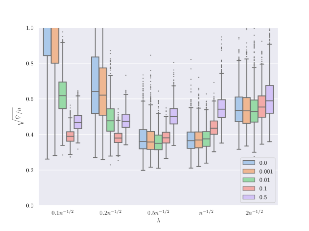
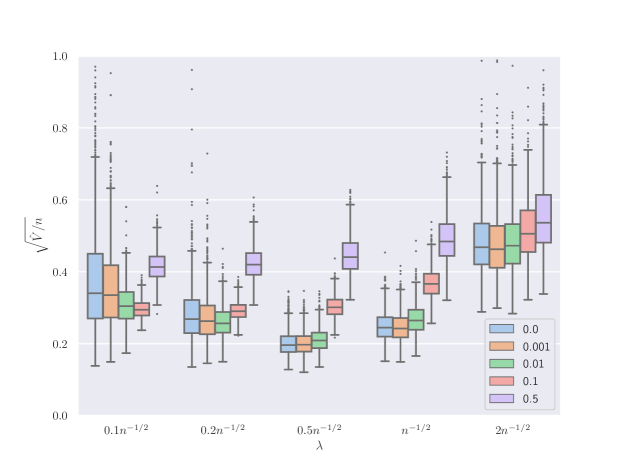
Figure 1: Boxplots of simulated $\hat{V}^{1/2}n^{-1/2}$. The simulation setup is described in Section 2.6. The top plot corresponds to iid standard Cauchy noise $\varepsilon_{i}$. The noise in the second plot is iid from the t-distribution with 2 degrees of freedom. Different colors correspond to different values of $\tau\in\{0,10^{-3},10^{-2},0.1,0.5\}$. In the x-axis, $\lambda$ takes values in $\{0.1n^{-1/2},0.2n^{-1/2},0.5n^{-1/2},n^{-1/2},2n^{-1/2}\}$.

We set $n=200,p=300$, and generate $\varepsilon_{i}\sim N(0,1)$ and the coordinates of ${\bm{\beta}}$ from iid Bernoulli variables with parameter $0.1$. We compute 1000 simulations of the Z-score $\Omega_{jj}^{1/2}\xi_{j}^{\prime}$ from Theorem 2.1 for $j=1$ for the $M$-estimator with the Huber loss and the Elastic-Net penalty (2.16) with $\sigma=1$ and the four combinations $(\lambda,\tau)\in\{n^{-1/2},2n^{-1/2}\}\times\{0,0.1\}$. The covariance matrix $\bm{\Sigma}$ is set as $\bm{A}^{\top}\bm{A}/n$ where $\bm{A}\in\mathbb{R}^{2p\times p}$ has iid Rademacher entries; $\bm{\Sigma}$ is generated once and is the same across the 1000 simulations. The average value and standard error over the 1000 simulations of $\hat{n}$, $\hat{\mathsf{df}}$, $|\hat{S}|$ and $\hat{V}^{1/2}n^{-1/2}$ are presented in Table 2 for ${\bm{\varepsilon}}$ with iid standard Cauchy components and Table 3 for ${\bm{\varepsilon}}$ with iid components from the t-distribution with $2$ degrees of freedom, together with histograms and QQ-plots against standard normal quantiles of $\Omega_{jj}^{1/2}\xi_{j}^{\prime}$ in (2.15).

The quantity $\hat{V}^{1/2}n^{-1/2}=\|\bm{\psi}\|_{2}/(\hat{n}-\hat{\mathsf{df}})$ featured in the boxplots of Figure 1 characterizes the length of our confidence intervals in (2.12). Computing the values $\hat{V}^{1/2}$ for different tuning parameters lets the practitioner pick the tuning parameters leading to the smallest confidence interval width, although this process amounts to the construction of multiple confidence intervals and warrants a Bonferroni multiple testing correction.

The histograms and QQ-plots in Table 2 and Table 3 confirm the normality of $\xi_{j}^{\prime}$ for these two heavy-tailed continuous noise distributions.

Since $\hat{n}-\hat{\mathsf{df}}$ appears in the denominator of $\hat{V}$, the length of confidence intervals can be large if $\hat{n}-\hat{\mathsf{df}}$ is nearly zero and the length is infinite if $\hat{n}-\hat{\mathsf{df}}=0$. This explains the large values and large variances observed in the boxplots of Figure 1 for small tuning parameters.

Appendix A Proof of the main result

A.1 Supporting propositions

The proof of Theorem 2.1 relies on the two intermediary results given below. Proposition A.1 will be proved in Appendix B and Lemma A.2 in Appendix C.

Proposition A.1.

Let $n\geq 3$, $R>0$ and $\bm{z}\sim\text{\rm Unif}(\mathbb{S}^{n-1}(R))$, where $\mathbb{S}^{n-1}(R)$ is sphere of radius $R$ in $\mathbb{R}^{n}$. Assume either:

• $\bm{f}$ is locally Lipschitz on $\mathbb{S}^{n-1}(R)$ with $\mathbb{E}[\|\nabla\bm{f}(\bm{z})^{\top}\|_{F}^{2}]<\infty$.

• $\bm{f}(\bm{z})$ is of the form ${\widetilde{\bm{f}}}(\bm{z})/\|{\widetilde{\bm{f}}}(\bm{z})\|_{2}$ where ${\widetilde{\bm{f}}}:\mathbb{R}^{n}\to\mathbb{R}^{n}$ is locally Lipschitz and satisfies $\mathbb{P}(\|\bm{f}(\bm{z})\|_{2}\neq 0)=1$ and $\mathbb{E}[\|{\widetilde{\bm{f}}}(\bm{z})\|_{2}^{-2}\|\nabla{\widetilde{\bm{f}}}(\bm{z})\|_{F}^{2}]<+\infty$.

Define $\bm{P}_{\bm{z}}^{\perp}=\bm{I}_{n}-\bm{z}\bm{z}^{\top}/\|\bm{z}\|_{2}^{2}$ and $\xi_{\bm{f}}(\bm{z})=\bm{f}(\bm{z})^{\top}\bm{z}-R^{2}n^{-1}\operatorname*{tr}(\nabla\bm{f}(\bm{z})^{\top}\bm{P}_{\bm{z}}^{\perp})$. Then

$$\mathbb{E}\bigl{[}\bigl{(}\xi_{\bm{f}}(\bm{z})-\mathbb{E}[\bm{f}(\bm{z})]^{\top}\bm{z}\bigr{)}^{2}\bigr{]} \leq 2R^{4}(n^{2}-2n)^{-1}\mathbb{E}[\|\nabla\bm{f}(\bm{z})^{\top}\bm{P}_{\bm{z}}^{\perp}\|_{F}^{2}],$$ (A.1)

$$\mathbb{E}\bigl{[}\big{|}\|\bm{f}(\bm{z})\|_{2}-\|\mathbb{E}[\bm{f}(\bm{z})]\|_{2}\big{|}\bigr{]}^{2} \leq R^{2}(n-2)^{-1}\mathbb{E}[\|\nabla\bm{f}(\bm{z})^{\top}\bm{P}_{\bm{z}}^{\perp}\|_{F}^{2}].$$ (A.2)

Lemma A.2.

Let Assumptions A, B and C be fulfilled. Let $\eta_{n}=\sqrt{2\log(n)/n}+n^{-1/2}$,

$$\mathscr{E}_{j}=\{\|\bm{X}\bm{Q}_{j}\bm{\Sigma}^{-1/2}n^{-1/2}\|_{\text{op}}\leq 1+\sqrt{p/n}+\eta_{n}\}\cap\{\big{|}n^{-1/2}\Omega_{jj}^{1/2}\|\bm{z}_{j}\|_{2}-1\big{|}\leq\eta_{n}\},\ j\in[p],$$

$u_{*}=\bigl{[}K^{2}(1-1/n)(L\tau^{-1}\|\bm{\Sigma}\|_{\text{op}}(2+\sqrt{p/n}+2\eta_{n})^{2}+1)^{-1}-3L/n\bigr{]}_{+}$, and $\mathbb{E}_{j}$ be the conditional expectation given $(\|\bm{z}_{j}\|_{2},\bm{X}\bm{Q}_{j},{\bm{\varepsilon}})$. Then, when $u_{*}>0$

$$\sup_{\delta>0}\mathbb{E}\Bigl{[}\frac{n}{\|\bm{\psi}\|_{2}^{2}+\delta}\sum_{j\in[p]}I_{\mathscr{E}_{j}}h_{j}^{2}\Bigr{]}^{1/2}\leq\frac{\bigl{[}(1+\sqrt{\frac{p}{n}})^{2}+\frac{1}{n}\bigr{]}^{1/2}}{\phi_{\min}(\bm{\Sigma})^{1/2}(1-\eta_{n})_{+}^{2}u_{*}}+\frac{\bigl{[}\frac{2p}{n\tau}+\mathbb{E}[\|\bm{h}\|_{2}^{2}]\bigr{]}^{1/2}}{u_{*}^{1/2}}.$$ (A.3)

A.2 Proof of the main result

of Theorem 2.1.

Since $\bm{\psi}\neq{\bm{0}}_{n}$ for almost every $\bm{X}$ by Proposition D.2, $\xi_{j}$ is well-defined with $\mathbb{P}$-probability 1. By Lemma A.2 and the monotone convergence theorem as $\delta\to 0$ for the left-hand side (A.3), when $u_{*}>0$

$$\mathbb{E}\Bigl{[}\frac{n}{\|\bm{\psi}\|_{2}^{2}}\sum_{j\in[p]}I_{\mathscr{E}_{j}}h_{j}^{2}\Bigr{]}\leq\frac{\bigl{[}(1+\sqrt{\frac{p}{n}})^{2}+\frac{1}{n}\bigr{]}^{1/2}}{\phi_{\min}(\bm{\Sigma})^{1/2}(1-\eta_{n})_{+}^{2}u_{*}}+\frac{\bigl{[}\frac{2p}{n\tau}+\mathbb{E}[\|\bm{h}\|_{2}^{2}]\bigr{]}^{1/2}}{u_{*}^{1/2}}.$$

Under our assumptions, $\|\bm{\Sigma}\|_{\rm op}\leq{1/\kappa}<+\infty$ and $\mathbb{E}[\|\bm{\Sigma}^{1/2}\bm{h}\|_{2}^{2}]\leq\mathscr{R}<+\infty$, so that there exists some finite constant $\mathscr{N}>0$ and $\mathscr{A}<+\infty$ independent of $n,p$, such that for $n\geq\mathscr{N}$,

$$\sum_{j\in[p]}\mathbb{E}\Big{[}n\|\bm{\psi}\|_{2}^{-2}I_{\mathscr{E}_{j}}h_{j}^{2}\Big{]}\leq\mathscr{A}<+\infty.$$ (A.4)

By Markov’s inequality with respect to the uniform distribution on $[p]=\{1,...,p\}$, the set

$$J_{n,p}\coloneqq\bigl{\{}j\in[p]:\mathbb{E}\bigl{[}nI_{\mathscr{E}_{j}}\|\bm{\psi}\|_{2}^{-2}h_{j}^{2}\bigr{]}\leq\mathscr{A}/a_{p}\bigr{\}}\quad\text{ satisfies }\quad|J_{n,p}|/p\geq 1-a_{p}/p.$$ (A.5)

In this paragraph, for a given, fixed value of $({\bm{\varepsilon}},\bm{X}\bm{Q}_{j})$ we view $\bm{\psi}$ as a function of $\bm{z}_{j}$,

$$\bm{\psi}:\mathbb{R}^{n}\to\mathbb{R}^{n},\qquad\bm{\psi}:\bm{z}_{j}\mapsto\bm{\psi}(\bm{z}_{j})=\bm{\psi}({\bm{\varepsilon}},\bm{X}\bm{Q}_{j}+\bm{z}_{j}\bm{e}_{j}^{\top})$$ (A.6)

instead of (2.8), and we denote its Jacobian by $\nabla\bm{\psi}(\bm{z}_{j})^{\top}$ at any point $\bm{z}_{j}$ where (A.6) is Fréchet differentiable. Next, we argue conditionally on $(\bm{X}\bm{Q}_{j},\|\bm{z}_{j}\|_{2})$: Since $\bm{z}_{j}/\|\bm{z}_{j}\|_{2}$ is independent of $(\|\bm{z}_{j}\|_{2},\bm{X}\bm{Q}_{j})$ and by rotational invariance of the Gaussian distribution, conditionally on $(\|\bm{z}_{j}\|_{2},\bm{X}\bm{Q}_{j})$ the vector $\bm{z}_{j}$ is uniformly distributed on the sphere $\mathbb{S}^{n-1}(\|\bm{z}_{j}\|_{2})$. Let $\mathbb{E}_{j}$ denote the conditional expectation of $\bm{z}_{j}$ given $(\bm{X}\bm{Q}_{j},\|\bm{z}_{j}\|_{2})$. By Proposition C.4, the above function is locally Lipschitz. From Proposition C.4 (iii) we have that

$$I_{\mathscr{E}_{j}}\mathbb{E}_{j}[\|\bm{\psi}\|_{2}^{-2}\|\nabla\bm{\psi}(\bm{z}_{j})\|_{F}^{2}]\leq L(n\tau)^{-1}+I_{\mathscr{E}_{j}}\mathbb{E}_{j}[nL^{2}\|\bm{\psi}\|_{2}^{-2}h_{j}^{2}]$$ (A.7)

and the right-hand side is finite with probability one with respect to $(\bm{X}\bm{Q}_{j},\|\bm{z}_{j}\|_{2})$ thanks to (A.4) and Tonelli’s theorem for non-negative measurable functions. By Proposition D.2, conditional on almost every $(\bm{X}\bm{Q}_{j},\|\bm{z}_{j}\|_{2})$, $\bm{\psi}(\bm{z}_{j})\neq{\bm{0}}_{n}$ for almost every $\bm{z}_{j}\in\mathbb{R}$. We are now in position to apply Proposition A.1 with $\bm{f}=\bm{\psi}/\|\bm{\psi}\|_{2}$, $\bm{z}=\bm{z}_{j}$ and

$$\xi_{\bm{f}}(\bm{z}_{j}):=\|\bm{\psi}\|_{2}^{-1}\bigl{(}\bm{\psi}^{\top}\bm{z}_{j}-(\|\bm{z}_{j}\|_{2}^{2}/n)\operatorname*{tr}\bigl{[}\bm{P}_{\bm{\psi}}^{\perp}(\nabla\bm{\psi}(\bm{z}_{j}))^{\top}\bm{P}_{\bm{z}_{j}}^{\perp}\bigr{]}\bigr{)},$$

where $\bm{P}_{\bm{v}}^{\perp}:=\bm{I}_{n}-\bm{P}_{\bm{v}}$ with $\bm{P}_{\bm{v}}:=\bm{v}\bm{v}^{\top}/\|\bm{v}\|_{2}^{2}$ for any $\bm{v}\in\mathbb{R}^{n}$. By Proposition A.1 and (A.7),

$$I_{\mathscr{E}_{j}}\mathbb{E}_{j}[(\xi_{\bm{f}}(\bm{z}_{j})-\mathbb{E}_{j}[\bm{f}(\bm{z}_{j})]^{\top}\bm{z}_{j})^{2}]$$

$$\leq 2I_{\mathscr{E}_{j}}\|\bm{z}_{j}\|_{2}^{4}(n^{2}-2n)^{-1}\mathbb{E}_{j}[\|(\nabla\bm{f}(\bm{z}_{j}))^{\top}\bm{P}_{\bm{z}_{j}}^{\perp}\|_{F}^{2}]$$

$$\leq 2(1+\eta_{n})^{4}(1-2/n)^{-1}I_{\mathscr{E}_{j}}\Omega_{jj}^{-2}\mathbb{E}_{j}[\|\bm{\psi}\|_{2}^{-2}\|\nabla\bm{\psi}(\bm{z}_{j})\|_{F}^{2}]$$

$$\leq 2(1+\eta_{n})^{4}(1-2/n)^{-1}\kappa^{-2}\bigl{(}L(n\tau)^{-1}+I_{\mathscr{E}_{j}}\mathbb{E}_{j}[nL^{2}\|\bm{\psi}\|_{2}^{-2}h_{j}^{2}]\bigr{)}$$

and

$$I_{\mathscr{E}_{j}}(\|\mathbb{E}_{j}[\bm{f}(\bm{z}_{j})]\|_{2}-1)^{2}$$

$$\leq I_{\mathscr{E}_{j}}\|\bm{z}_{j}\|_{2}^{2}(n-2)^{-1}\mathbb{E}_{j}[\|(\nabla\bm{f}(\bm{z}_{j}))^{\top}\bm{P}_{\bm{z}_{j}}^{\perp}\|_{F}^{2}].$$

$$\leq(1+\eta_{n})^{2}(1-2/n)^{-1}I_{\mathscr{E}_{j}}\Omega_{jj}^{-1}\mathbb{E}_{j}[\|\bm{\psi}\|_{2}^{-2}\|\nabla\bm{\psi}(\bm{z}_{j})\|_{F}^{2}]$$

$$\leq(1+\eta_{n})^{2}(1-2/n)^{-1}\kappa^{-1}\bigl{(}L(n\tau)^{-1}+I_{\mathscr{E}_{j}}\mathbb{E}_{j}[nL^{2}\|\bm{\psi}\|_{2}^{-2}h_{j}^{2}]\bigr{)},$$

where the upper bounds follow from $I_{\mathscr{E}_{j}}\|\bm{z}_{j}\|_{2}^{4}\leq(1+\eta_{n})^{4}n^{2}\Omega_{jj}^{-2}$. Taking $\mathbb{E}$ on both sides, we obtain $\max_{j\in J_{n,p}}\mathbb{E}\bigl{[}I_{\mathscr{E}_{j}}(\xi_{\bm{f}}(\bm{z}_{j})-\mathbb{E}_{j}[\bm{f}(\bm{z}_{j})]^{\top}\bm{z}_{j})^{2}+I_{\mathscr{E}_{j}}|\|\mathbb{E}_{j}[\bm{f}(\bm{z}_{j})]\|_{2}-1|\bigr{]}\to 0$. Thanks to $\min_{j\in[p]}\mathbb{P}(\mathscr{E}_{j})\to 1$ by Lemma C.1 this implies that both $|\|\mathbb{E}_{j}[\bm{f}(\bm{z}_{j})]\|_{2}-1|$ and $|\xi_{\bm{f}}(\bm{z}_{j})^{\top}\bm{z}_{j})-\mathbb{E}_{j}[\bm{f}(\bm{z}_{j})]^{\top}\bm{z}_{j}|$ converge in probability to 0 uniformly over $j\in J_{n,p}$.

We now study the asymptotic distribution of $\xi_{\bm{f}}(\bm{z}_{j})$. Since $\bm{z}_{j}\sim N({\bm{0}}_{n},\Omega_{jj}^{-1}\bm{I}_{n})$ is independent with $\bm{X}\bm{Q}_{j}$ by Proposition D.1, without loss of generality, we can assume that $\bm{z}_{j}=\|\bm{z}_{j}\|_{2}\bm{\zeta}_{j}/\|\bm{\zeta}_{j}\|_{2}$ for some $\bm{\zeta}_{j}\sim N({\bm{0}}_{n},\bm{I}_{n})$ independent of $(\bm{X}\bm{Q}_{j},\|\bm{z}_{j}\|_{2})$. Then $\mathbb{E}_{j}$ coincides with the conditional expectation of $\bm{\zeta}_{j}$ given $(\bm{X}\bm{Q}_{j},\|\bm{z}_{j}\|_{2})$. After some rearrangement,

$$\xi_{\bm{f}}(\bm{z}_{j})=\xi_{\bm{f}}(\bm{z}_{j})-\mathbb{E}_{j}[\bm{f}(\bm{z}_{j})]^{\top}\bm{z}_{j}+\|\mathbb{E}_{j}[\bm{f}(\bm{z}_{j})]\|_{2}\frac{\|\bm{z}_{j}n^{-1/2}\|_{2}}{\|\bm{\zeta}_{j}n^{-1/2}\|_{2}}\Bigl{(}\frac{\mathbb{E}_{j}[\bm{f}(\bm{z}_{j})]}{\|\mathbb{E}_{j}[\bm{f}(\bm{z}_{j})]\|_{2}}\Bigr{)}^{\top}\bm{\zeta}_{j}.$$

Uniformly over $j\in J_{n,p}$, we have (i) $|\xi_{\bm{f}}(\bm{z}_{j})-\mathbb{E}_{j}[\bm{f}(\bm{z}_{j})]^{\top}\bm{z}_{j}|\to 0$ and $\|\mathbb{E}_{j}[\bm{f}(\bm{z}_{j})]\|_{2}\to 1$ in probability, (ii) $\frac{\mathbb{E}_{j}[\bm{f}(\bm{z}_{j})]^{\top}}{\|\mathbb{E}_{j}[\bm{f}(\bm{z}_{j})]\|_{2}}\bm{\zeta}_{j}\sim N(0,1)$ and (iii) $\|\Omega_{jj}^{1/2}\bm{z}_{j}\|_{2}/\|\bm{\zeta}_{j}\|_{2}\to 1$ in probability. By Slutsky’s Theorem, $\Omega_{jj}^{1/2}\xi_{\bm{f}}(\bm{z}_{j})$ converges in distribution to $N(0,1)$ uniformly over $j\in J_{n,p}$. That is, for any $t\in\mathbb{R}$, $\max_{j\in J_{n,p}}|\mathbb{P}(\Omega_{jj}^{1/2}\xi_{\bm{f}}(\bm{z}_{j})\leq t)-\Phi(t)|\to 0.$

It remains to relate $\xi_{\bm{f}}(\bm{z}_{j})$ to $\xi_{j}$ defined in (2.9). As the term $\|\bm{\psi}\|_{2}^{-1}\bm{z}_{j}^{\top}\bm{\psi}$ present in both $\xi_{j}$ and $\xi_{\bm{f}}(\bm{z}_{j})$ cancel out, we have the decomposition

$$\|\bm{\psi}\|_{2}\|\bm{z}_{j}\|_{2}^{-2}n\bigl{(}\xi_{j}-\xi_{\bm{f}}(\bm{z}_{j})\bigr{)}$$

$$=(\widehat{\beta}_{j}-\beta_{j})\operatorname*{tr}[\nabla_{\bm{y}}\bm{\psi}^{\top}]+\operatorname*{tr}(\bm{P}_{\bm{\psi}}^{\perp}(\nabla\bm{\psi}(\bm{z}_{j}))^{\top}\bm{P}_{\bm{z}_{j}}^{\perp})$$ (A.8)

$$=\operatorname*{tr}\bigl{[}\bigl{(}(\widehat{\beta}_{j}-\beta_{j})\nabla_{\bm{y}}\bm{\psi}^{\top}+\nabla\bm{\psi}(\bm{z}_{j})^{\top}\big{)}\bm{P}_{\bm{\psi}}^{\perp}\bigr{]}$$ (A.9)

$$\qquad\quad+(\widehat{\beta}_{j}-\beta_{j})\operatorname*{tr}\bigl{[}\bm{P}_{\bm{\psi}}\nabla_{\bm{y}}\bm{\psi}^{\top}\bigr{]}+\operatorname*{tr}\bigl{[}\bm{P}_{\bm{\psi}}^{\perp}\nabla\bm{\psi}(\bm{z}_{j})^{\top}\bm{P}_{\bm{z}_{j}}\bigr{]}.$$ (A.10)

The matrix inside the trace in (A.8) is zero thanks to (C.25). It follows that only the two terms in (A.10) remain, hence

$$\mathbb{E}[I_{\mathscr{E}_{j}}(\xi_{j}-\xi_{\bm{f}}(\bm{z}_{j}))^{2}]\leq(2/n)\mathbb{E}\bigl{[}I_{\mathscr{E}_{h}}\|\bm{z}_{j}\|_{2}^{2}\|\bm{\psi}\|_{2}^{-2}\bigl{(}(\widehat{\beta}_{j}-\beta_{j})^{2}\|\nabla_{\bm{y}}\bm{\psi}\|_{\text{op}}^{2}+\|\nabla\bm{\psi}(\bm{z}_{j})\|_{\text{op}}^{2}\bigr{)}\bigr{]}.$$

Since $I_{\mathscr{E}_{j}}\|\bm{z}_{j}\|^{2}/n\leq\Omega_{jj}^{-1}(1+\eta_{n})^{2}$ and $\|\nabla_{\bm{y}}\bm{\psi}\|_{\rm op}\leq L$ by Proposition C.4 (i) with $\bm{X}={{\smash{\widetilde{\bm{X}}}}}$, the first term is bounded from above by $L\Omega_{jj}^{-1}(1+\eta_{n})^{2}\mathbb{E}[I_{\mathscr{E}_{j}}\|\bm{\psi}\|_{2}^{-2}h_{j}^{2}]$ which converges to 0 uniformly over $j\in J_{n,p}$ by definition of $J_{n,p}$ in (A.5). The second term also converges to 0 uniformly over $j\in J_{n,p}$ thanks to (A.7). Thus $\max_{j\in J_{n,p}}\mathbb{E}[I_{\mathscr{E}_{j}}(\xi_{j}-\xi_{\bm{f}}(\bm{z}_{j}))^{2}]\to 0$ which implies that $|\xi_{j}-\xi_{\bm{f}}(\bm{z}_{j})|\to 0$ in probability uniformly over $j\in J_{n,p}$ and Slutsky’s theorem completes the proof of (2.11) for $\xi_{j}$.

To prove a similar result for $\xi_{j}^{\prime}$, it is enough to prove $\Omega_{j}^{1/2}|\xi_{j}^{\prime}-\xi_{j}|\to^{\mathbb{P}}0$ uniformly over $j\in J_{n,p}$ by Slutsky’s theorem. As $|\xi_{j}-\xi_{j}^{\prime}|=\big{|}\operatorname*{tr}[\nabla_{\bm{y}}\bm{\psi}]\big{|}\|\bm{\psi}\|_{2}^{-1}\big{|}h_{j}\big{|}~{}\big{|}\|\bm{z}_{j}\|_{2}^{2}/n-\Omega_{jj}^{-1}\big{|}$ and $|\operatorname*{tr}[\nabla_{\bm{y}}\bm{\psi}]|\leq nL$, by the Cauchy-Schwarz inequality we find

$$\mathbb{E}[I_{\mathscr{E}_{j}}|\xi_{j}-\xi_{j}^{\prime}|]\leq\Omega_{jj}^{-1}nL\mathbb{E}[I_{\mathscr{E}_{j}}h_{j}^{2}\|\bm{\psi}\|_{2}^{-2}]^{1/2}\mathbb{E}[(\Omega_{jj}\|\bm{z}_{j}\|_{2}^{2}/n-1)^{2}]^{1/2}.$$

Since $\mathbb{E}[(\Omega_{jj}\|\bm{z}_{j}\|_{2}^{2}/n-1)^{2}]^{1/2}=\sqrt{2/n}$ and $\Omega_{jj}\in[\kappa,1/\kappa]$, the previous display converges to 0 uniformly over $j\in J_{n,p}$ by definition of $J_{n,p}$ in (A.5). ∎

Appendix B Stein formulae on the sphere

The goal of this section is to prove Proposition A.1 and to develop Stein formulae for random vectors $\bm{z}$ uniformly distributed on the sphere.

Let $\mathbb{S}^{n-1}(R)$ be the sphere in $\mathbb{R}^{n}$ with center ${\bm{0}}$ and radius $R>0$. We say that $\bm{z}$ is uniformly distributed in $\mathbb{S}^{n-1}(R)$ and write $\bm{z}\sim\text{\rm Unif}(\mathbb{S}^{n-1}(R))$ if $\bm{z}$ is equal in distribution to $R\bm{\zeta}/\|\bm{\zeta}\|_{2}$ where $\bm{\zeta}\sim N(\mathbf{0},\bm{I}_{n})$. We first develops Stein’s formulae with respect to $\bm{z}\sim\text{\rm Unif}(\mathbb{S}^{n-1}(R))$ for functions $\bm{f}:\bm{z}\in\mathbb{S}^{n-1}(R)\mapsto\bm{f}(\bm{z})\in\mathbb{R}^{n}$ in Sobolev spaces over $\mathbb{S}^{n-1}(R)$.

We derive next Stein formulae for functions in Sobolev spaces over $\mathbb{S}^{n-1}(R)$. One possible construction of such Sobolev spaces is obtained by completion of the space of infinitely differentiable functions $\mathbb{S}^{n-1}(R)\to\mathbb{R}$ with respect to the desired Sobolev norm as follows. Here, $\mathbb{S}^{n-1}(R)$ is viewed as a compact Riemannian manifold equipped with the canonical metric (the metric induced as a submanifold of $\mathbb{R}^{n}$ equipped with the Euclidean metric). As it will be convenient for compatibility with the rest of the paper to conserve the partial derivatives with respect to the canonical basis in $\mathbb{R}^{n}$, we adopt the following notation. For a smooth function $h:\mathbb{S}^{n-1}(R)\to\mathbb{R}$ and $\Omega\subset\mathbb{R}^{n}$ an open neighborhood of $\mathbb{S}^{n-1}(R)$, define the smooth function $\check{h}:\Omega\to\mathbb{R}$ by $\check{h}(\bm{x})=h(R\bm{x}/\|\bm{x}\|_{2})$ and define the gradient of $h$ as that of $\check{h}$, i.e., for $\bm{x}\in\mathbb{S}^{n-1}(R)$, set $\nabla h(\bm{x})=((\partial/\partial x_{1})\check{h}(\bm{x}),...,(\partial/\partial x_{n})\check{h}(\bm{x}))$. For every $\bm{x}\in\mathbb{S}^{n-1}$, the gradient $\nabla h(\bm{x})$ belongs to the hyperplane orthogonal to $\bm{x}$ which is the tangent space of $\mathbb{S}^{n-1}$ at $\bm{x}$. Furthermore if $\bm{\gamma}:\mathbb{R}\to\mathbb{S}^{n-1}(R)$ is a smooth curve with $\bm{\gamma}(0)=\bm{x},(d/dt)\bm{\gamma}(t)|_{t=0}=\bm{v}$ then $\bm{v}^{\top}\bm{x}=0$ and $\nabla h(\bm{x})^{\top}\bm{v}=(d/dt)h(\bm{\gamma}(t))|_{t=0}$. For such smooth function $h$ and equipped with its gradient, for $\alpha\in\{1,2\}$ we define the Sobolev norm

$$\|h\|_{1,\alpha}=\mathbb{E}\bigl{[}|h(\bm{z})|^{\alpha}\bigr{]}^{1/\alpha}+\mathbb{E}\bigl{[}\|\nabla h(\bm{z})\|_{2}^{\alpha}\bigr{]}^{1/\alpha},\qquad\bm{z}\sim\text{\rm Unif}(\mathbb{S}^{n-1}(R))$$

and the Sobolev space $W^{1,\alpha}(\mathbb{S}^{n-1}(R))$ as the completion of the space of smooth functions over $\mathbb{S}^{n-1}(R)$ with respect to the above norm. This definition is equivalent to the definition given in [18, Definition 2.1]. By [18, Proposition 2.3], since the manifold $\mathbb{S}^{n-1}(R)$ is compact the resulting Sobolev spaces do not depend on the chosen metric. Equivalently, the Sobolev space $W^{1,\alpha}(\mathbb{S}^{n-1}(R))$ is also the completion with respect to the above norm of the space of once continuously differentiable functions on $\mathbb{S}^{n-1}(R)$.

If $h$ is locally Lipschitz on $\mathbb{S}^{n-1}(R)$ (i.e., every point has a neighborhood in $\mathbb{S}^{n-1}(R)$ on which $h$ is Lipschitz), then again by considering an open neighborhood $\Omega\subset\mathbb{R}^{n}$ of $\mathbb{S}^{n-1}(R)$, the function $\check{h}(\bm{x})=h(R\bm{x}/\|\bm{x}\|_{2})$ is locally Lipschitz on $\Omega$. Thus, in this case and by Rademacher’s theorem, $\nabla h(\bm{z})$ is well defined almost everywhere in $\mathbb{S}^{n-1}(R)$ as the gradient of $\nabla\check{h}(\bm{x})$, and $h\in W^{1,\alpha}(\mathbb{S}^{n-1}(R))$ if and only if $\mathbb{E}\big{[}\|\nabla h(\bm{z})\|_{2}^{\alpha}\big{]}<\infty$. For example, $h\in W^{1,\alpha}(\mathbb{S}^{n-1}(R))$ when $h$ is $L$-Lipschitz on $\mathbb{S}^{n-1}(R)$.

Finally, for $\alpha\in\{1,2\}$ define $W^{1,\alpha}(\mathbb{S}^{n-1}(R))^{n}$ as the space of $\mathbb{R}^{n}$ valued functions $\bm{f}=(f_{1},...,f_{n})$ with all coordinates $f_{i}$ belonging to $W^{1,\alpha}(\mathbb{S}^{n-1}(R))$, equipped with the norm

$$\|\bm{f}\|_{1,\alpha}=\mathbb{E}[\|\bm{f}(\bm{z})\|_{2}^{\alpha}]^{1/\alpha}+\mathbb{E}[\|\nabla\bm{f}(\bm{z})\|_{F}^{\alpha}]^{1/\alpha}$$

where the gradient $\nabla\bm{f}$ is the matrix in $\mathbb{R}^{n\times n}$ with columns $\nabla f_{1},...,\nabla f_{n}$,

Lemma B.1 (Stein’s formula on the sphere).

Let $n\geq 3$, $R>0$ and $\bm{z}\sim\text{\rm Unif}(\mathbb{S}^{n-1}(R))$. Let $\bm{P}_{\bm{x}}^{\perp}=\bm{I}_{n}-\bm{x}\bm{x}^{\top}/\|\bm{x}\|_{2}^{2}$ for $\bm{x}\neq{\bf 0}$. Then, for all $\bm{f}=(f_{1},\ldots,f_{n})\in W^{1,1}(\mathbb{S}^{n-1}(R))^{n}$,

$$\mathbb{E}[\bm{f}(\bm{z})^{\top}\bm{z}]=(n-1)^{-1}R^{2}\mathbb{E}[\operatorname*{tr}((\nabla\bm{f}(\bm{z}))^{\top}\bm{P}_{\bm{z}}^{\perp})],$$ (B.1)

where $\nabla\bm{f}=(\nabla f_{1},\ldots,\nabla f_{n})$. Moreover, for all $\bm{f}=(f_{1},\ldots,f_{n})\in W^{1,1}(\mathbb{S}^{n-1}(R))^{n}$,

$$\mathbb{E}[\|\bm{f}(\bm{z})-\mathbb{E}[\bm{f}(\bm{z})]\|_{2}^{2}]\leq(n-2)^{-1}R^{2}\mathbb{E}[\|\nabla\bm{f}(\bm{z})^{\top}\bm{P}_{\bm{z}}^{\perp}\|_{F}^{2}],$$ (B.2)

$$\mathbb{E}\bigl{[}\bigl{(}nR^{-2}\bm{f}(\bm{z})^{\top}\bm{z}-\operatorname*{tr}[\nabla\bm{f}(\bm{z})^{\top}\bm{P}_{\bm{z}}^{\perp}]\bigr{)}^{2}\bigr{]}$$

$$=nR^{-2}\mathbb{E}\bigl{[}\|\bm{f}\|_{2}^{2}\bigr{]}+n(n-2)^{-1}\mathbb{E}\operatorname*{tr}\bigl{[}\bigl{(}\nabla\bm{f}(\bm{z})^{\top}\bm{P}_{\bm{z}}^{\perp}\bigr{)}^{2}\bigr{]}-2(n-2)^{-1}\mathbb{E}\bigl{[}\operatorname*{tr}(\nabla f(\bm{z})^{\top}\bm{P}_{\bm{z}}^{\perp})^{2}\bigr{]}$$ (B.3)

$$\leq nR^{-2}\mathbb{E}\bigl{[}\|\bm{f}\|_{2}^{2}\bigr{]}+(1-2/n)^{-1}\mathbb{E}\bigl{[}\|\nabla\bm{f}(\bm{z})^{\top}\bm{P}_{\bm{z}}^{\perp}\|_{F}^{2}\bigr{]}.$$ (B.4)

Note that (B.2) is the classical Poincaré inequality on the sphere. A proof is provided for completeness.

of Lemma B.1.

As the operators $T$ and $T_{ij}$ defined by $T\bm{f}(\bm{z})=\bm{f}(\bm{z})^{\top}\bm{z}$ and $T_{ij}\bm{f}(\bm{z})=[\nabla\bm{f}(\bm{z})^{\top}\bm{P}_{\bm{z}}^{\perp}]_{ij}$ for every $i,j=1,...,n$ are all continuous linear mappings from $W^{1,\alpha}(\mathbb{S}^{n-1}(R))^{n}$ to the $L_{\alpha}$ space with the norm $\|f\|_{L_{\alpha}}=(\mathbb{E}[|f(\bm{z})|^{\alpha}])^{1/\alpha}$, we assume without loss of generality that all coordinates of $\bm{f}$ are continuously differentiable. Indeed, if $(\bm{f}^{(q)})_{q\geq 1}$ is a sequence of smooth functions over the sphere converging to $\bm{f}$ in $W^{1,\alpha}(\mathbb{S}^{n-1}(R))^{n}$ for $\alpha=1$ and (B.1) holds for $\bm{f}^{(q)}$ then (B.1) also holds for the limit by continuity; the same argument applies with $\alpha=2$ for (B.2)-(B.3)-(B.4).

Let $\bm{\zeta}\sim N(\mathbf{0},\bm{I}_{n})$. Assume without loss of generality $\bm{z}=R\bm{\zeta}/\|\bm{\zeta}\|_{2}$ as $R\bm{\zeta}/\|\bm{\zeta}\|_{2}\sim\text{\rm Unif}(\mathbb{S}^{n-1}(R))$. Let $\phi(t)$ be a continuously differentiable function in $\mathbb{R}$ with $\phi(t)=0$ for $t\leq 0$ and $\phi(t)=1$ for $t\geq 1$. For $\delta>0$ define $\bm{\varphi}_{\delta}(\bm{x})=\phi(\|\bm{x}\|_{2}/\delta)\bm{f}(R\bm{x}/\|\bm{x}\|_{2})$. As $\|\bm{\zeta}\|_{2}$ is independent of $\bm{z}$ and $\bm{\varphi}_{\delta}(\bm{x})$ has uniformly bounded gradient, the first order Stein formula for $\bm{\varphi}_{\delta}$ yields

$$\mathbb{E}\big{[}\phi(\|\bm{\zeta}\|_{2}/\delta)\|\bm{\zeta}\|_{2}\big{]}\mathbb{E}[\bm{f}(\bm{z})^{\top}\bm{z}]=\mathbb{E}\big{[}R\bm{\varphi}_{\delta}(\bm{\zeta})^{\top}\bm{\zeta}\big{]}=R\,\mathbb{E}\big{[}\operatorname*{tr}(\nabla\bm{\varphi}_{\delta}(\bm{\zeta}))\big{]}.$$

By the product and chain rules, $\nabla\bm{\varphi}_{\delta}(\bm{x})$ is given by

$$\phi^{\prime}(\|\bm{x}\|_{2}/\delta)(\bm{x}/(\|\bm{x}\|_{2}\delta))\bm{f}(R\bm{x}/\|\bm{x}\|_{2})^{\top}+\phi(\|\bm{x}\|_{2}/\delta)(R/\|\bm{x}\|_{2})\bm{P}_{\bm{x}}^{\perp}\big{(}\nabla\bm{f}(R\bm{x}/\|\bm{x}\|_{2})\big{)}$$

with $\phi^{\prime}(t)=(d/dt)\phi(t)$ and $\phi^{\prime}(0)=\phi^{\prime}(1)=0$. As $\sup_{\delta>0,\bm{x}\in\mathbb{R}^{n}}\|\bm{x}\|_{2}\|\nabla\bm{\varphi}_{\delta}(\bm{x})\|_{\rm F}\leq C<\infty$ and $\mathbb{E}[\|\bm{\zeta}\|_{2}^{-2}]=1/(n-2)<\infty$, the dominated convergence theorem gives

$$\mathbb{E}[\bm{f}(\bm{z})^{\top}\bm{z}]=\frac{R\lim_{\delta\to 0}\mathbb{E}\big{[}\operatorname*{tr}(\nabla\bm{\varphi}_{\delta}(\bm{\zeta}))\big{]}}{\lim_{\delta\to 0}\mathbb{E}\big{[}\phi(\|\bm{\zeta}\|_{2}/\delta)\|\bm{\zeta}\|_{2}\big{]}}=\frac{R^{2}\mathbb{E}\big{[}1/\|\bm{\zeta}\|_{2}\big{]}\mathbb{E}\big{[}\operatorname*{tr}(\nabla\bm{f}(\bm{z})^{\top}\bm{P}_{\bm{z}}^{\perp})\big{]}}{\mathbb{E}\big{[}\|\bm{\zeta}\|_{2}\big{]}},$$

which yields (B.1) due to $\mathbb{E}[\|\bm{\zeta}\|_{2}]/\mathbb{E}[\|\bm{\zeta}\|_{2}^{-1}]=(n-1)$.

Next, as the exchange of limit and expectation is allowed when $\bm{\varphi}_{\delta}\to\bm{\varphi}_{0+}=\bm{f}$, the Gaussian Poincaré inequality [9, Theorem 1.6.4] yields

$$\mathbb{E}[\|\bm{f}(\bm{z})-\mathbb{E}[\bm{f}(\bm{z})]\|_{2}^{2}]\leq\lim_{\delta\to 0+}\mathbb{E}[\|\nabla\bm{\varphi}_{\delta}(\bm{\zeta})\|_{F}^{2}]=\mathbb{E}[R^{2}\|\nabla\bm{f}(\bm{z})^{\top}\bm{P}_{\bm{z}}^{\perp}\|_{F}^{2}\|\bm{\zeta}\|_{2}^{-2}].$$

Since $\mathbb{E}[\|\bm{\zeta}\|_{2}^{-2}]=1/(n-2)$ and $(\|\bm{\zeta}\|_{2},\bm{z})$ are independent, we obtain (B.2). Finally by applying the Second Order Stein formula of [5] to $\bm{\varphi}_{\delta}(\bm{\zeta})$ we find by dominated convergence

$$\mathbb{E}\bigl{[}\bigl{(}R^{-1}\|\bm{\zeta}\|_{2}\bm{z}^{\top}\bm{f}(\bm{z})-R\|\bm{\zeta}\|_{2}^{-1}\operatorname*{tr}[\nabla\bm{f}(\bm{z})^{\top}\bm{P}_{\bm{z}}^{\perp}]\bigr{)}^{2}\bigr{]}$$

$$=\lim_{\delta\to 0^{+}}\mathbb{E}\bigl{[}\bigl{(}\bm{\zeta}^{\top}\bm{\varphi}_{\delta}(\bm{\zeta})-\operatorname*{tr}[\nabla\bm{\varphi}_{\delta}(\bm{\zeta})]\bigr{)}^{2}\bigr{]}$$

$$=\lim_{\delta\to 0^{+}}\mathbb{E}\bigl{[}\|\bm{\varphi}_{\delta}(\bm{\zeta})\|_{2}^{2}\bigr{]}+\mathbb{E}\operatorname*{tr}\bigl{[}\bigl{(}\nabla\bm{\varphi}_{\delta}(\bm{\zeta})^{\top}\bigr{)}^{2}\bigr{]}$$

$$=\mathbb{E}\bigl{[}\|\bm{f}(\bm{z})\|_{2}^{2}\bigr{]}+R^{2}\mathbb{E}\operatorname*{tr}\bigl{[}\bigl{(}\nabla\bm{f}(\bm{z})^{\top}\bm{P}_{\bm{z}}^{\perp}\bigr{)}^{2}\bigr{]}\mathbb{E}\bigl{[}\|\bm{\zeta}\|_{2}^{-2}\bigr{]}$$

$$=\mathbb{E}\bigl{[}\|\bm{f}(\bm{z})\|_{2}^{2}\bigr{]}+R^{2}\mathbb{E}\operatorname*{tr}\bigl{[}\bigl{(}\nabla\bm{f}(\bm{z})^{\top}\bm{P}_{\bm{z}}^{\perp}\bigr{)}^{2}\bigr{]}/(n-2),$$

where the last equality follows from the independence of $\bm{z}$ and $\|\bm{\zeta}\|_{2}$. We now simplify the left-hand side in order to get rid of $\|\bm{\zeta}\|_{2}$. By expanding the square and using the independence of $(\bm{z},\|\bm{\zeta}\|_{2})$, the above display is equal to

$$R^{-2}\mathbb{E}[\|\bm{\zeta}\|_{2}^{2}]\mathbb{E}[(\bm{z}^{\top}\bm{f}(\bm{z}))^{2}]-2\mathbb{E}\bigl{[}\bm{z}^{\top}\bm{f}(\bm{z})\operatorname*{tr}[\nabla\bm{f}(\bm{z})^{\top}\bm{P}_{\bm{z}}^{\perp}]\bigr{]}+R^{2}\mathbb{E}[\|\bm{\zeta}\|_{2}^{-2}]\mathbb{E}\bigl{[}(\operatorname*{tr}[\nabla\bm{f}(\bm{z})^{\top}\bm{P}_{\bm{z}}^{\perp}])^{2}\bigr{]}$$

$$=nR^{-2}\mathbb{E}[(\bm{z}^{\top}\bm{f}(\bm{z}))^{2}]-2\mathbb{E}\bigl{[}\bm{z}^{\top}\bm{f}(\bm{z})\operatorname*{tr}[\nabla\bm{f}(\bm{z})^{\top}\bm{P}_{\bm{z}}^{\perp}]\bigr{]}+R^{2}(n-2)^{-1}\mathbb{E}\bigl{[}(\operatorname*{tr}[\nabla\bm{f}(\bm{z})^{\top}\bm{P}_{\bm{z}}^{\perp}])^{2}\bigr{]}$$

$$=\mathbb{E}\Bigl{[}\Bigl{(}\frac{\sqrt{n}}{R}\bm{z}^{\top}\bm{f}(\bm{z})-\frac{R}{\sqrt{n}}\operatorname*{tr}[\nabla\bm{f}(\bm{z})^{\top}\bm{P}_{\bm{z}}^{\perp}]\Bigr{)}^{2}\Bigr{]}+R^{2}\Bigl{(}\frac{1}{n-2}-\frac{1}{n}\Bigr{)}\mathbb{E}\Bigl{[}\big{(}\operatorname*{tr}[\nabla\bm{f}(\bm{z})^{\top}\bm{P}_{\bm{z}}^{\perp}]\big{)}^{2}\Bigr{]}.$$

Since $1/(n-2)-1/n=2n^{-1}(n-2)^{-1}$, we obtain (B.3) after multiplying by $n/R^{2}$. The proof is complete since (B.4) follows directly from (B.3) by the Cauchy-Schwarz inequality. ∎

of Proposition A.1.

If $\bm{f}$ is locally Lipschitz and $\mathbb{E}[\|\nabla\bm{f}(\bm{z})^{\top}\|_{F}^{2}]<\infty$, then $\bm{f}\in W^{1,2}(\mathbb{S}^{n-1}(R))$. We consider the mapping $\bm{f}(\bm{z})-\mathbb{E}\bigl{[}\bm{f}(\bm{z})\bigr{]}$ rather than $\bm{f}(\bm{z})$ in (B.3) and (B.4). Multiplying $R^{4}n^{-2}$ on both sides of the inequality (B.4), it provides

$$\mathbb{E}[(\xi_{\bm{f}}(\bm{z})-\mathbb{E}[\bm{f}(\bm{z})]^{\top}\bm{z})^{2}] \leq R^{2}n^{-1}\mathbb{E}[\|\bm{f}-\mathbb{E}[\bm{f}(\bm{z})]\|_{2}^{2}]+R^{4}(n^{2}-2n)^{-1}\mathbb{E}[\|\nabla\bm{f}(\bm{z})^{\top}\bm{P}_{\bm{z}}^{\perp}\|_{F}^{2}]$$

$$\leq 2R^{4}(n^{2}-2n)^{-1}\mathbb{E}[\|\nabla\bm{f}(\bm{z})^{\top}\bm{P}_{\bm{z}}^{\perp}\|_{F}^{2}],$$

where the second inequality follows from (B.2). By the triangle inequality and (B.2),

$$\mathbb{E}[|\|\bm{f}(\bm{z})\|_{2}-\|\mathbb{E}[\bm{f}(\bm{z})]\|_{2}|^{2}] \leq\mathbb{E}[\|\bm{f}(\bm{z})-\mathbb{E}[\bm{f}(\bm{z})]\|_{2}^{2}]$$

$$\leq R^{2}(n-2)^{-1}\mathbb{E}[\|\nabla\bm{f}(\bm{z})^{\top}\bm{P}_{\bm{z}}^{\perp}\|_{F}^{2}].$$

If $\bm{f}(\bm{z})={\widetilde{\bm{f}}}(\bm{z})/\|{\widetilde{\bm{f}}}(\bm{z})\|_{2}$ with locally Lipschitz ${\widetilde{\bm{f}}}$ on $\mathbb{S}^{n-1}(R)$ then ${\widetilde{\bm{f}}}(\bm{z})/(\delta\vee\|{\widetilde{\bm{f}}}(\bm{z})\|_{2})$ is locally Lipschitz for $\delta>0$ and converges to $\bm{f}$ in $W^{1,2}(\mathbb{S}^{n-1}(R))^{n}$ as $\delta\to 0+$ when $\mathbb{P}(\|\bm{f}(\bm{z})\|_{2}\neq 0)=1$ and $\mathbb{E}[\|{\widetilde{\bm{f}}}(\bm{z})\|_{2}^{-2}\|\nabla{\widetilde{\bm{f}}}(\bm{z})\|_{F}^{2}]<+\infty$. Thus, the proof still applies. ∎

Appendix C Bounds on $(\widehat{\beta}_{j}-\beta_{j})^{2}\|\mathbf{\psi}\|_{2}^{-2}$

The goal of this section is to prove Lemma A.2.

C.1 High probability events $\mathscr{E}_{j}$

Lemma C.1 (high probability of $\mathscr{E}_{j}$).

Assume that $\bm{X}$ has iid $N({\bm{0}},\bm{\Sigma})$ rows. Then

$$\mathbb{E}[\|\bm{X}\bm{\Sigma}^{-1/2}\|_{\text{op}}^{2}]\leq(\sqrt{n}+\sqrt{p})^{2}+1.$$ (C.1)

Furthermore, with $\eta_{n}=\sqrt{2\log(n)/n}+n^{-1/2}$ and for the events

$$\mathscr{E}_{j}=\{\|\bm{X}\bm{Q}_{j}\bm{\Sigma}^{-1/2}n^{-1/2}\|_{\text{op}}\leq 1+\sqrt{p/n}+\eta_{n}\}\cap\{\big{|}n^{-1/2}\Omega_{jj}^{1/2}\|\bm{z}_{j}\|_{2}-1\big{|}\leq\eta_{n}\},$$

we have $\mathbb{P}(\cap_{j\in[p]}\mathscr{E}_{j})\geq 1-(p+1/2)n^{-1}(\pi\log(n))^{-1/2}$.

of Lemma C.1.

Let us first notice that $\bm{X}\bm{\Sigma}^{-1/2}$ is a random Gaussian matrix with iid standard normal entries. Theorem 7.3.1 in [31] provides that $\mathbb{E}[\|\bm{X}\bm{\Sigma}^{-1/2}\|_{\text{op}}]\leq\sqrt{n}+\sqrt{p}$. Since the operator norm of a matrix is a 1-Lipschitz function of the entries of the matrix, by the Gaussian Poincaré inequality [10, Theorem 3.20], ${\rm Var}(\|\bm{X}\bm{\Sigma}^{-1/2}\|_{\text{op}})\leq 1.$ This proves (C.1).

By Theorem II.13 in [14], we have for $t>0$,

$$\mathbb{P}(\|\bm{X}\bm{\Sigma}^{-1/2}n^{-1/2}\|_{\text{op}}\geq 1+\sqrt{p/n}+t)\leq\Phi(-t\sqrt{n}),$$

$$\mathbb{P}(\big{|}\Omega_{jj}^{1/2}\|\bm{z}_{j}n^{-1/2}\|_{2}-1\big{|}\geq n^{-1/2}+t)\leq 2\Phi(-t\sqrt{n}).$$

Since $\bm{X}\bm{Q}_{j}\bm{\Sigma}^{-1/2}=\bm{X}\bm{\Sigma}^{-1/2}(\bm{\Sigma}^{1/2}\bm{Q}_{j}\bm{\Sigma}^{-1/2})$ and $\|\bm{\Sigma}^{1/2}\bm{Q}_{j}\bm{\Sigma}^{-1/2}\|_{\text{op}}\leq 1$, $\|\bm{X}\bm{Q}_{j}\bm{\Sigma}^{-1/2}\|_{\text{op}}\leq\|\bm{X}\bm{\Sigma}^{-1/2}\|_{\text{op}}$ for all $j\in[p]$. With this we can conclude the above inequalities using a union bound over $j\in[p]$ when $t=\sqrt{2\log(n)/n}$, $\mathbb{P}(\cap_{j\in[p]}\mathscr{E}_{j})\geq 1-(2p+1)\Phi(-\sqrt{2\log(n)}).$ Thanks to $\Phi(-t)\leq(2\pi)^{-1/2}\exp(-t^{2}/2)/t$ for $t>0$, we have

$$\mathbb{P}(\cap_{j\in[p]}\mathscr{E}_{j})\geq 1-(p+1/2)n^{-1}(\pi\log(n))^{-1/2}.$$

∎

Remark C.1.

Our specific construction of $\mathscr{E}_{j}$ satisfies the following properties:

1. $I_{\mathscr{E}_{j}}$ is a function of $\|\bm{X}\bm{Q}_{j}\|_{\text{op}}$ and $\|\bm{z}_{j}\|_{2}$ only, consequently the event $\mathscr{E}_{j}$ is independent of $\bm{z}_{j}/\|\bm{z}_{j}\|_{2}$.

2. $\|\bm{X}\bm{\Sigma}^{-1/2}n^{-1/2}\|_{\text{op}}I_{\mathscr{E}_{j}}\leq 1+\sqrt{p/n}+\eta_{n}+(1+\eta_{n})=2+\sqrt{p/n}+2\eta_{n}.$

C.2 Twice continuously differentiable penalty

Lemma C.2.

Let $L,\tau$ be such that Assumptions A and B are fulfilled. Further assume that the Hessian matrix $\bm{G}=(\nabla^{2}g())\big{|}_{\hat{{\bm{\beta}}}}$ of $g$ at $\hat{{\bm{\beta}}}$ exists and is symmetric, and define

$$\bm{M} =(\bm{X}^{\top}\operatorname*{diag}(\bm{\psi}^{\prime})\bm{X}+n\bm{G})^{-1},$$ (C.2)

$$\bm{V} =\operatorname*{diag}(\bm{\psi}^{\prime})-\operatorname*{diag}(\bm{\psi}^{\prime})\bm{X}\bm{M}\bm{X}^{\top}\operatorname*{diag}(\bm{\psi}^{\prime}).$$ (C.3)

Then with the partial order $\bm{A}\preceq\bm{B}$ if and only if the matrix $\bm{B}-\bm{A}$ is positive semi-definite, we have

$$\|\operatorname*{diag}(\bm{\psi}^{\prime})\bm{X}\bm{M}\|_{\text{op}} \leq(1/2)L^{1/2}(n\tau)^{-1/2},$$ (C.4)

$$\bm{M} \preceq(n\tau)^{-1}\bm{I}_{p},$$ (C.5)

$$(L\tau^{-1}\|\bm{X}n^{-1/2}\|_{\text{op}}^{2}+1)^{-1}\operatorname*{diag}(\bm{\psi}^{\prime}) \preceq\bm{V}\preceq\operatorname*{diag}(\bm{\psi}^{\prime})\preceq L\bm{I}_{n}.$$ (C.6)

of Lemma C.2.

Throughout the proof we denote by $\bm{B}=\operatorname*{diag}(\bm{\psi}^{\prime})^{1/2}\bm{X}n^{-1/2}\bm{G}^{-1/2}$. By some algebra, we have $\bm{B}(\bm{B}^{\top}\bm{B}+\bm{I}_{p})^{-1}\bm{B}^{\top}=\operatorname*{diag}(\bm{\psi}^{\prime})^{1/2}\bm{X}\bm{M}\bm{X}^{\top}\operatorname*{diag}(\bm{\psi}^{\prime})^{1/2}$. For an upper bound of $\operatorname*{diag}(\bm{\psi}^{\prime})\bm{X}\bm{M}$, we notice

$$\operatorname*{diag}(\bm{\psi}^{\prime})\bm{X}\bm{M} =\operatorname*{diag}(\bm{\psi}^{\prime})\bm{X}(\bm{X}^{\top}\operatorname*{diag}(\bm{\psi}^{\prime})\bm{X}+n\bm{G})^{-1}$$

$$=\operatorname*{diag}(\bm{\psi}^{\prime})^{1/2}\bm{B}(\bm{B}^{\top}\bm{B}+\bm{I}_{p})^{-1}n^{-1/2}\bm{G}^{-1/2}.$$

For any matrix $\bm{B}$, $\|\bm{B}(\bm{B}^{\top}\bm{B}+\bm{I}_{p})^{-1}\|_{\text{op}}\leq\max_{t\geq 0}t/(t^{2}+1)=1/2$. By strongly convexity of $g$, $\|\bm{G}^{-1/2}\|_{\text{op}}\leq\tau^{-1/2}$. Since $\psi$ is $L$-Lipschitz, $\|\operatorname*{diag}(\bm{\psi}^{\prime})^{1/2}\|_{\text{op}}\leq L^{1/2}$. Combining those upper bounds, we obtain (C.4). For the upper bound of $\bm{M}$, we notice $\bm{M}=n^{-1}\bm{G}^{-1/2}(\bm{B}^{\top}\bm{B}+\bm{I}_{p})^{-1}\bm{G}^{-1/2}\preceq n^{-1}\bm{G}^{-1}\preceq(n\tau)^{-1}\bm{I}_{p}.$ This gives (C.5). For lower and upper bounds on $\bm{V}$, we first notice that by definition of $\bm{B}$, $\|\bm{B}\|_{\text{op}}\leq L^{1/2}\tau^{-1/2}\|\bm{X}n^{-1/2}\|_{\text{op}},$ thus

$$(L\tau^{-1}\|\bm{X}n^{-1/2}\|_{\text{op}}^{2}+1)^{-1}\bm{I}_{n}\preceq\bm{I}_{n}-\bm{B}(\bm{B}^{\top}\bm{B}+\bm{I}_{p})^{-1}\bm{B}^{\top}\preceq\bm{I}_{n}.$$

Since $\bm{V}=\operatorname*{diag}(\bm{\psi}^{\prime})^{1/2}(\bm{I}_{n}-\bm{B}(\bm{B}^{\top}\bm{B}+\bm{I}_{p})^{-1}\bm{B}^{\top})\operatorname*{diag}(\bm{\psi}^{\prime})^{1/2}$, we have

$$(L\tau^{-1}\|\bm{X}n^{-1/2}\|_{\text{op}}^{2}+1)^{-1}\operatorname*{diag}(\bm{\psi}^{\prime})\preceq\bm{V}\preceq\operatorname*{diag}(\bm{\psi}^{\prime}).$$

By the $L$-Lipschitz property of $\psi$, we have $\operatorname*{diag}(\bm{\psi}^{\prime})\preceq L\bm{I}_{n}$. Thus (C.6) holds. ∎

Proposition C.3.

Assume that $g$ is strongly convex with parameter $\tau>0$ and $\psi=\rho^{\prime}$ is $L$-Lipschitz. Let $\hat{{\bm{\beta}}}=\hat{{\bm{\beta}}}({\bm{\varepsilon}},\bm{X})$ be as in (2.2). Let $\bm{\psi}({\bm{\varepsilon}},\bm{X})=\bm{\psi}$, $\bm{\psi}^{\prime}$ and $\bm{h}({\bm{\varepsilon}},\bm{X})=\hat{{\bm{\beta}}}-{\bm{\beta}}$ be as in (2.6). Define $\nabla_{\bm{z}}\bm{h}=(\partial/\partial\bm{z})\bm{h}({\bm{\varepsilon}},\bm{X}+\bm{z}^{\top})\big{|}_{\bm{z}=0}$ and $\nabla_{\bm{z}}\bm{\psi}=(\partial/\partial\bm{z})\bm{\psi}({\bm{\varepsilon}},\bm{X}+\bm{z}^{\top})\big{|}_{\bm{z}=0}$ for fixed , ${\bm{\varepsilon}}$ and $\bm{X}$. Let $\bm{P}_{\bm{x}}^{\perp}=\bm{I}_{n}-\bm{x}\bm{x}^{\top}/\|\bm{x}\|_{2}^{2}$ for $\bm{x}\neq{\bf 0}$. Then

(i) For fixed ${\bm{\varepsilon}}$, $\bm{h}({\bm{\varepsilon}},\bm{X})$ and $\bm{\psi}({\bm{\varepsilon}},\bm{X})$ are Lipschitz in $\bm{X}$ on every compact subset of $\mathbb{R}^{n\times p}$.

For (ii) and (iii), additionally assume that $g$ is twice continuously differentiable.

(ii) For almost every $\bm{X}$ and every $\in\mathbb{R}^{p}$,

$$(\nabla_{\bm{z}}\bm{h})^{\top}=-(\bm{h}^{\top})\bm{M}\bm{X}^{\top}\operatorname*{diag}(\bm{\psi}^{\prime})+\bm{M}\bm{\psi}^{\top},$$ (C.7)

$$(\nabla_{\bm{z}}\bm{\psi})^{\top}=-(\bm{h}^{\top})\bm{V}-\operatorname*{diag}(\bm{\psi}^{\prime})\bm{X}\bm{M}\bm{\psi}^{\top}.$$ (C.8)

(iii) For almost every $\bm{X}$ and every $\in\mathbb{R}^{p}$, if $\bm{\psi}\neq\mathbf{0}$, then

$$(\nabla_{\bm{z}}(\bm{\psi}/\|\bm{\psi}\|_{2}))^{\top}=\|\bm{\psi}\|_{2}^{-1}\bm{P}^{\perp}_{\bm{\psi}}\big{[}-(\bm{h}^{\top})\bm{V}-\operatorname*{diag}(\bm{\psi}^{\prime})\bm{X}\bm{M}\bm{\psi}^{\top}\big{]}$$ (C.9)

We remark that in view of (A.6), $\nabla_{\bm{z}}\bm{\psi}=\nabla\bm{\psi}(\bm{z}_{j})$ when $\bm{e}_{j}$.

Proof.

(i) We refer our readers to the proof of Proposition C.4.

(ii) As the functions $\bm{h}$ and $\bm{\psi}$ are Lipschitz on every compact, their Fréchet derivatives exist almost everywhere by Rademacher’s theorem. Moreover, the chain rule holds almost everywhere by [33, Theorem 2.1.11]. Let $\bm{G},\bm{V}$ and $\bm{M}$ be as in Lemma C.2. By differentiating these KKT conditions $\bm{X}^{\top}\bm{\psi}(\bm{X})=n(\nabla g())\big{|}_{{\bm{\beta}}+\bm{h}}$, and by the chain rule, we obtain that for almost every $\bm{X}$,

$$n\bm{G}\big{(}\nabla_{\bm{z}}\bm{h}\big{)}^{\top}=\bm{\psi}^{\top}+\bm{X}^{\top}\big{(}\nabla_{\bm{z}}\bm{\psi}\big{)}^{\top},\quad\big{(}\nabla_{\bm{z}}\bm{\psi}\big{)}^{\top}=\operatorname*{diag}(\bm{\psi}^{\prime})\big{\{}-(^{\top}\bm{h})\bm{I}_{n}-\bm{X}\big{(}\nabla_{\bm{z}}\bm{h}\big{)}^{\top}\big{\}}.$$

Solving the above system of equations gives (C.7) and (C.8).

(iii) Since the map $\bm{v}\mapsto\bm{v}/\|\bm{v}\|_{2}$ with $\bm{v}\in\mathbb{R}^{n}$ has Fréchet derivative $\|\bm{v}\|_{2}^{-1}\bm{P}_{\bm{v}}^{\perp}$ at every point $\bm{v}\neq{\bm{0}}\in\mathbb{R}^{n}$, by chain rule, (C.9) follows for almost every $\bm{X}$ if $\bm{\psi}(\bm{X})\neq{\bm{0}}_{n}$. ∎

of Lemma A.2 when $g$ is twice continuously differentiable.

Here, we further assume that $g$ is twice differentiable so that $\bm{V},\bm{M}$ in Lemma C.2 are well-defined.

By Proposition C.4, the map $\bm{z}_{j}\mapsto(\bm{h},\bm{\psi})$ is locally Lipschitz, thus the map of the product $\bm{z}_{j}\mapsto h_{j}\bm{\psi}(\|\bm{\psi}\|_{2}^{2}+\delta)^{-1}$ is also locally Lipschitz. By Proposition D.2, without loss of generality, we can assume that $\bm{\psi}\neq{\bm{0}}_{n}$ at almost every point $\bm{z}_{j}\in\mathbb{R}^{n}$. By the first order Stein’s formula on the sphere (B.1) for $(n-1)\|\bm{z}_{j}\|_{2}^{-2}\mathbb{E}_{j}[\bm{z}_{j}^{\top}\bm{f}(\bm{z}_{j})]$ with $\bm{f}(\bm{z}_{j})=h_{j}\bm{\psi}(\|\bm{\psi}\|_{2}^{2}+\delta)^{-1}$, we have

$$\mathbb{E}_{j}[h_{j}^{2}(\|\bm{\psi}\|_{2}^{2}+\delta)^{-1}\operatorname*{tr}(\bm{V}\bm{P}_{\bm{z}_{j}}^{\perp})]$$ (C.10)

$$= -\mathbb{E}_{j}[h_{j}(\|\bm{\psi}\|_{2}^{2}+\delta)^{-1}\bm{\psi}^{\top}\bm{z}_{j}](n-1)\|\bm{z}_{j}\|_{2}^{-2}$$ (C.11)

$$-2\mathbb{E}_{j}[h_{j}(\|\bm{\psi}\|_{2}^{2}+\delta)^{-1}\bm{e}_{j}^{\top}(\operatorname*{diag}(\bm{\psi}^{\prime})\bm{X}\bm{M})^{\top}\bm{P}_{\bm{z}_{j}}^{\perp}\bm{\psi}]$$ (C.12)

$$+\mathbb{E}_{j}[(\|\bm{\psi}\|_{2}^{2}+\delta)^{-1}\bm{e}_{j}^{\top}\bm{M}\bm{e}_{j}\bm{\psi}^{\top}\bm{P}_{\bm{z}_{j}}^{\perp}\bm{\psi}]$$ (C.13)

$$+2\mathbb{E}_{j}[h_{j}^{2}(\|\bm{\psi}\|_{2}^{2}+\delta)^{-2}\bm{\psi}^{\top}\bm{V}\bm{P}_{\bm{z}_{j}}^{\perp}\bm{\psi}]$$ (C.14)

$$+2\mathbb{E}_{j}[h_{j}(\|\bm{\psi}\|_{2}^{2}+\delta)^{-2}\bm{\psi}^{\top}\operatorname*{diag}(\bm{\psi}^{\prime})\bm{X}\bm{M}\bm{e}_{j}\bm{\psi}^{\top}\bm{P}_{\bm{z}_{j}}^{\perp}\bm{\psi}].$$ (C.15)

For the terms (C.12)-(C.14), by Lemma C.2 and $\|\bm{P}_{\bm{z}_{j}}^{\perp}\|_{{\rm op}}\leq 1$ we find

$$\eqref{eq:3254_term2}\vee\eqref{eq:3254_term5} \leq\sqrt{L/(\tau n)}\mathbb{E}_{j}[|h_{j}|(\|\bm{\psi}\|_{2}^{2}+\delta)^{-1/2}]$$ by (C.4)

$$\leq\tfrac{1}{2}(\tau n)^{-1}+\tfrac{L}{2}\mathbb{E}_{j}[h_{j}^{2}(\|\bm{\psi}\|_{2}^{2}+\delta)^{-1}],$$

$$\eqref{eq:3254_term3} \leq(\tau n)^{-1} \text{by \eqref{eq:M-bound}},$$

$$\eqref{eq:3254_term4} \leq 2L\mathbb{E}_{j}[h_{j}^{2}(\|\bm{\psi}\|_{2}^{2}+\delta)^{-1}] \text{by \eqref{eq:V-bound}}.$$

By leaving term (C.11) unchanged and using the above inequalities,

$$\eqref{eq:3254}\leq -(n-1)\|\bm{z}_{j}\|_{2}^{-2}\mathbb{E}_{j}[h_{j}(\|\bm{\psi}\|_{2}^{2}+\delta)^{-1}\bm{\psi}^{\top}\bm{z}_{j}]$$ (C.16)

$$+2(\tau n)^{-1}$$

$$+3L\mathbb{E}_{j}[h_{j}^{2}(\|\bm{\psi}\|_{2}^{2}+\delta)^{-1}].$$

We now bound (C.10) from below. Let

$$U_{j}=(L\tau^{-1}(\|\bm{X}\bm{Q}_{j}n^{-1/2}\|_{\text{op}}+\|\bm{z}_{j}n^{-1/2}\|_{2})^{2}+1)^{-1}.$$

By $(L\tau^{-1}\|\bm{X}n^{-1/2}\|_{\text{op}}^{2}+1)^{-1}\operatorname*{diag}(\bm{\psi}^{\prime})\preceq\bm{V}\preceq\operatorname*{diag}(\bm{\psi}^{\prime})\preceq L\bm{I}_{n}$ in (C.6) and by $\|\bm{X}\|_{\text{op}}\leq\|\bm{X}\bm{Q}_{j}\|_{\text{op}}+\|\bm{z}_{j}\|_{2}$ for all $j\in[p]$, we have that $U_{j}\operatorname*{diag}(\bm{\psi}^{\prime})\preceq\bm{V}\preceq L\bm{I}_{n}$.

Since $U_{j}\operatorname*{diag}(\bm{\psi}^{\prime})\preceq\bm{V}$ and $K^{2}\bm{I}_{n}\preceq\operatorname*{diag}(\bm{\psi}^{\prime})+\operatorname*{diag}\{\psi_{i}^{2},i=1,...,n\}$ both holds, multiplying the second inequality by $U_{j}$ and summing yields $K^{2}U_{j}\bm{I}_{n}\preceq U_{j}\operatorname*{diag}\psi_{i}^{2}+\bm{V}$. Multiplying both sides $\bm{P}_{\bm{z}_{j}}^{\perp}$ to the left and to the right and using that $\bm{P}_{\bm{z}_{j}}^{\perp}\preceq\bm{I}_{n}$ and $\operatorname*{tr}\bm{P}_{\bm{z}_{j}}^{\perp}=n-1$ we find

$$K^{2}U_{j}\bm{P}_{\bm{z}_{j}}^{\perp}\preceq U_{j}\operatorname*{diag}\psi_{i}^{2}+\bm{P}_{\bm{z}_{j}}^{\perp}\bm{V}\bm{P}_{\bm{z}_{j}}^{\perp},\qquad K^{2}U_{j}(n-1)\leq U_{j}\|\bm{\psi}\|^{2}+\operatorname*{tr}[\bm{P}_{\bm{z}_{j}}^{\perp}\bm{V}].$$

Multiplying by $(\|\bm{\psi}\|_{2}^{2}+\delta)^{-1}h_{j}^{2}$ and taking the conditional expectation $\mathbb{E}_{j}$,

$$K^{2}U_{j}(n-1)\mathbb{E}_{j}[(\|\bm{\psi}\|_{2}^{2}+\delta)^{-1}h_{j}^{2}] \leq\mathbb{E}_{j}[h_{j}^{2}]+\mathbb{E}_{j}[\operatorname*{tr}[\bm{P}_{\bm{z}_{j}}^{\perp}\bm{V}]h_{j}^{2}(\|\bm{\psi}\|_{2}^{2}+\delta)^{-1}]$$ (C.17)

$$=\mathbb{E}_{j}[h_{j}^{2}]+\eqref{eq:3254}.$$ (C.18)

Note that by definition of $u_{*}$ and the events in Lemma C.1, we have when $u_{*}>0$,

$$\mathscr{E}_{j}\subset\{nu_{*}\leq K^{2}U_{j}(n-1)-3L\}\cap\{\Omega_{jj}\|\bm{z}_{j}\|_{2}^{2}\geq n(1-\eta_{n})_{+}^{2}\}.$$ (C.19)

Then combining (C.16) with the previous display, multiplying both sides by $I_{\mathscr{E}_{j}}$ and summing over $j\in[p]$ we find

$$nu_{*}\sum_{j=1}^{p}\mathbb{E}_{j}\Bigl{[}\frac{I_{\mathscr{E}_{j}}h_{j}^{2}}{\|\bm{\psi}\|_{2}^{2}+\delta}\Bigr{]}\leq\frac{2p}{\tau n}+\sum_{j=1}^{p}\mathbb{E}_{j}[I_{\mathscr{E}_{j}}h_{j}^{2}]-(n-1)\mathbb{E}_{j}\Bigl{[}\frac{\bm{\psi}^{\top}\bm{z}_{j}I_{\mathscr{E}_{j}}\bm{e}_{j}^{\top}\bm{h}}{(\|\bm{\psi}\|_{2}^{2}+\delta)\|\bm{z}_{j}\|_{2}^{2}}\Bigr{]}.$$

Taking expectations $\mathbb{E}$, letting $\operatorname*{diag}\{I_{\mathscr{E}_{j}}\}$ denote the diagonal matrix with the $j$-th diagonal element $I_{\mathscr{E}_{j}}$, we find

$$nu_{*}\mathbb{E}\bigl{[}(\|\bm{\psi}\|_{2}^{2}+\delta)^{-1}\bm{h}^{\top}\operatorname*{diag}\{I_{\mathscr{E}_{j}}\}\bm{h}\bigr{]}-2p/(\tau n)-\mathbb{E}[\|\bm{h}\|_{2}^{2}]$$

$$\leq-(n-1)\mathbb{E}\bigl{[}(\|\bm{\psi}\|_{2}^{2}+\delta)^{-1}\bm{\psi}^{\top}\bm{X}\bm{\Sigma}^{-1}\operatorname*{diag}\{\Omega_{jj}^{-1}I_{\mathscr{E}_{j}}\|\bm{z}_{j}\|_{2}^{-2}\}\bm{h}\bigr{]}$$

$$\leq(n-1)\mathbb{E}\bigl{[}\|\bm{X}\bm{\Sigma}^{-1}\operatorname*{diag}\{\Omega_{jj}^{-1}I_{\mathscr{E}_{j}}\|\bm{z}_{j}\|_{2}^{-2}\}\|_{\text{op}}^{2}\bigr{]}^{1/2}\mathbb{E}\bigl{[}(\|\bm{\psi}\|_{2}^{2}+\delta)^{-1}\bm{h}^{\top}\operatorname*{diag}\{I_{\mathscr{E}_{j}}\}\bm{h}\bigr{]}^{1/2}$$

$$\leq(1-\eta_{n})_{+}^{-2}\mathbb{E}\bigl{[}\|\bm{X}\bm{\Sigma}^{-1}\|_{\text{op}}^{2}\bigr{]}^{1/2}\mathbb{E}\bigl{[}(\|\bm{\psi}\|_{2}^{2}+\delta)^{-1}\bm{h}^{\top}\operatorname*{diag}\{I_{\mathscr{E}_{j}}\}\bm{h}\bigr{]}^{1/2}$$

where the second inequality follows from the Cauchy-Schwarz inequality and $(\|\bm{\psi}\|_{2}^{2}+\delta)^{-1/2}\|\bm{\psi}\|_{2}\leq 1$, and the third inequality follows from $\Omega_{jj}^{-1}I_{\mathscr{E}_{j}}(n-1)\|\bm{z}_{j}\|_{2}^{-2}\leq(1-\eta_{n})_{+}^{-2}$ thanks to (C.19). This implies that $x=(n\mathbb{E}[(\|\bm{\psi}\|_{2}^{2}+\delta)^{-1}\bm{h}^{\top}\operatorname*{diag}\{I_{\mathscr{E}_{j}}\}\bm{h}])^{1/2}$ satisfies $Ax^{2}+Bx+C\leq 0$ where the polynomial coefficients are $A=u_{*}$, $C=-2p(\tau n)^{-1}-\mathbb{E}[\|\bm{h}\|_{2}^{2}]$ and $B=-(1-\eta_{n})_{+}^{-2}\mathbb{E}[\|\bm{X}\bm{\Sigma}^{-1}n^{-1}\|_{\text{op}}^{2}]^{1/2}.$ As $A>0$, inequality $Ax^{2}+Bx+C\leq 0$ implies that $x$ lies between the two real roots of the polynomial $AX^{2}+BX+C$. In particular, $x$ is smaller than the largest root, i.e., $x\leq(-B+\sqrt{B^{2}-4AC})/(2A)\leq|B|/A+(|C|/A)^{1/2}$. Here, $|C|/A=(2p(n\tau)^{-1}+\mathbb{E}[\|\bm{h}\|_{2}^{2}])/u_{*}$ and

$$|B|/A\leq u_{*}^{-1}(1-\eta_{n})_{+}^{-2}\big{|}\|\bm{\Sigma}^{-1/2}\|_{\text{op}}\mathbb{E}[\|\bm{X}\bm{\Sigma}^{-1/2}n^{-1/2}\|_{\text{op}}^{2}]^{1/2}.$$

The upper bound (C.1) on $\mathbb{E}[\|\bm{X}\bm{\Sigma}^{-1/2}\|_{\text{op}}^{2}]$ completes the proof.

∎

C.3 Non-smooth strongly convex penalty $g$

C.3.1 Almost everywhere differentiability

In this section, we provide the almost everywhere existence of the Jacobian matrices. We also notice that if our penalty $g$ is not twice differentiable, the matrices $\bm{M}$ and $\bm{V}$ in Lemma C.2 are not well defined. In this case we do not have explicit formula for the Jacobian matrices $(\partial/\partial\bm{z}_{j})\bm{\psi}$ and $(\partial/\partial\bm{z}_{j})\bm{h}$ such as those in terms of $\bm{V},\operatorname*{diag}(\bm{\psi}^{\prime}),\bm{M}$ in Proposition C.3 (ii) and (iii). In this section we provide upper bounds of the norms of these Jacobian matrices without using Proposition C.3.

Proposition C.4.

Let $\rho:\mathbb{R}\to\mathbb{R}$ be convex and continuously differentiable with derivative $\psi=\rho^{\prime}$ being $L$-Lipschitz. Let $g:\mathbb{R}^{p}\to\mathbb{R}$ be strongly convex with parameter $\tau>0$. Let $\bm{X},{{\smash{\widetilde{\bm{X}}}}}\in\mathbb{R}^{n\times p}$, ${\bm{\varepsilon}},{\widetilde{{\bm{\varepsilon}}}}\in\mathbb{R}^{n}$ and correspondingly,

$$\hat{{\bm{\beta}}}({\bm{\varepsilon}},\bm{X}) =\operatorname*{argmin}_{\in\mathbb{R}^{p}}\sum_{i\in[n]}\frac{\rho(\varepsilon_{i}-\bm{x}_{i}^{\top}({\bm{\beta}}))}{n}+g(), \tilde{{\bm{\beta}}}=\hat{{\bm{\beta}}}({\widetilde{{\bm{\varepsilon}}}},{{\smash{\widetilde{\bm{X}}}}}),$$ (C.20)

$$\bm{h}({\bm{\varepsilon}},\bm{X}) =\hat{{\bm{\beta}}}({\bm{\varepsilon}},\bm{X})-{\bm{\beta}}, {\widetilde{\bm{h}}}=\bm{h}({\widetilde{{\bm{\varepsilon}}}},{{\smash{\widetilde{\bm{X}}}}}),$$

$$\bm{\psi}({\bm{\varepsilon}},\bm{X}) =\psi({\bm{\varepsilon}}-\bm{X}\bm{h}({\bm{\varepsilon}},\bm{X})), {\widetilde{\bm{\psi}}}=\bm{\psi}({\widetilde{{\bm{\varepsilon}}}},{{\smash{\widetilde{\bm{X}}}}}).$$

Then (i)

$$n\tau\|\bm{h}-{\widetilde{\bm{h}}}\|_{2}^{2}+L^{-1}\|\bm{\psi}-{\widetilde{\bm{\psi}}}\|_{2}^{2}\leq(\bm{h}-{\widetilde{\bm{h}}})^{\top}(\bm{X}-{{\smash{\widetilde{\bm{X}}}}})^{\top}\bm{\psi}+({\bm{\varepsilon}}-{\widetilde{{\bm{\varepsilon}}}}+{{\smash{\widetilde{\bm{X}}}}}\bm{h}-\bm{X}\bm{h})^{\top}(\bm{\psi}-{\widetilde{\bm{\psi}}}).$$ (C.21)

(ii) The map $({\bm{\varepsilon}},\bm{X})\mapsto\bigl{(}\bm{h}({\bm{\varepsilon}},\bm{X}),\bm{\psi}({\bm{\varepsilon}},\bm{X})\bigr{)}$ is Lipschitz on every compact of $\mathbb{R}^{n}\times\mathbb{R}^{n\times p}$.

(iii) For any ${\bm{\varepsilon}}\in\mathbb{R}^{n}$ fixed, and for any $\bm{\eta}\in\mathbb{R}^{n}$ and $\in\mathbb{R}^{p}$

$$n\tau\|\hat{{\bm{\beta}}}({\bm{\varepsilon}},\bm{X}+\bm{\eta}^{\top})-\hat{{\bm{\beta}}}({\bm{\varepsilon}},\bm{X})\|_{2}^{2}+L^{-1}\|\bm{\psi}({\bm{\varepsilon}},\bm{X}+\bm{\eta}^{\top})-\bm{\psi}({\bm{\varepsilon}},\bm{X})\|_{2}^{2}$$

$$\leq(n\tau)^{-1}\|\|_{2}^{2}(\bm{\eta}^{\top}\bm{\psi})^{2}+L(\bm{h}^{\top})^{2}\|\bm{\eta}\|_{2}^{2}.$$

Furthermore,

$$\sum_{i\in[n]}\|\bm{\psi}({\bm{\varepsilon}},\bm{X}+\bm{e}_{i}^{\top})-\bm{\psi}(\bm{X})\|_{2}^{2}\leq L(n\tau)^{-1}\|\|_{2}^{2}\|\bm{\psi}\|_{2}^{2}+nL^{2}(\bm{h}^{\top})^{2}.$$ (C.22)

(iv) If $\bm{\eta}\in\mathbb{R}^{n}$ is such that $\bm{\eta}^{\top}\bm{\psi}({\bm{\varepsilon}},\bm{X})=0$ then $\bm{\psi}({\bm{\varepsilon}}+\bm{h}({\bm{\varepsilon}},\bm{X})^{\top}\bm{e}_{j}\bm{\eta},\bm{X}+\bm{\eta}\bm{e}_{j}^{\top})=\bm{\psi}({\bm{\varepsilon}},\bm{X})$, so that if $\bm{\psi}({\bm{\varepsilon}},\bm{X})$ is Fréchet differentiable at $({\bm{\varepsilon}},\bm{X})$ then

$$\sum_{i=1}^{n}\eta_{i}\Big{[}\frac{\partial\bm{\psi}}{\partial x_{ij}}({\bm{\varepsilon}},\bm{X})+\Bigl{(}\bm{e}_{j}^{\top}\bm{h}({\bm{\varepsilon}},\bm{X})\Bigr{)}\frac{\partial\bm{\psi}}{\partial\varepsilon_{i}}({\bm{\varepsilon}},\bm{X})\Big{]}=0\quad\text{ provided that }\bm{\eta}^{\top}\bm{\psi}({\bm{\varepsilon}},\bm{X})=0.$$ (C.23)

The content of the above proposition appeared in [4, Proposition 5.2] with variables $(\bm{y},\bm{X})$ instead of $({\bm{\varepsilon}},\bm{X})$. It follows from strong convexity and the KKT conditions of $\hat{{\bm{\beta}}}$ and $\tilde{{\bm{\beta}}}$. Its proof is provided below for completeness. An application of the above Proposition C.4 to normalized $\bm{\psi}$ yields the following.

Corollary C.5.

Under the conditions of Proposition C.4 and with the notation of Proposition C.3, at a point where $\|\bm{\psi}\|_{2}>0$ and $\bm{\psi}$ is Fréchet differentiable,

$$\bigg{\|}\nabla_{\bm{z}}\bigg{(}\frac{\bm{\psi}}{\|\bm{\psi}\|_{2}}\bigg{)}\bigg{\|}_{F}^{2}\leq\frac{L\|\|_{2}^{2}}{n\tau}+\frac{nL^{2}(\bm{h}^{\top})^{2}}{\|\bm{\psi}\|_{2}^{2}},$$ (C.24)

and with the $\nabla_{\bm{y}}\bm{\psi}$ in (2.8)

$$\bigg{(}\nabla_{\bm{z}}\bigg{(}\frac{\bm{\psi}}{\|\bm{\psi}\|_{2}}\bigg{)}+\big{(}^{\top}\bm{h}\big{)}\frac{\nabla_{\bm{y}}\bm{\psi}}{\|\bm{\psi}\|_{2}}\bigg{)}^{\top}\bm{P}_{\bm{\psi}}^{\perp}={\bf 0}.$$ (C.25)

Proof.

For (C.24), by the chain rule $\|\nabla_{\bm{z}}(\bm{\psi}/\|\bm{\psi}\|_{2})^{\top}\|_{F}^{2}=\|\bm{\psi}\|_{2}^{-2}\|\bm{P}_{\bm{\psi}}^{\perp}(\nabla_{\bm{z}}\bm{\psi})^{\top}\|_{F}^{2}\leq\|\bm{\psi}\|_{2}^{-2}\|\nabla_{\bm{z}}\bm{\psi}\|_{F}^{2}$. By definition of the Frobenius norm $\|\nabla_{\bm{z}}\bm{\psi}\|_{F}^{2}=\sum_{i\in[n]}\|\partial\bm{\psi}/\partial z_{i}\|_{2}^{2}.$ By (C.22) with replaced by $t$ and taking the limit as $t\to 0$ we obtain $\|\nabla_{\bm{z}}(\bm{\psi}/\|\bm{\psi}\|_{2})\|_{F}^{2}\leq L(n\tau)^{-1}\|\|_{2}^{2}+nL^{2}(\bm{h}^{\top})^{2}\|\bm{\psi}\|_{2}^{-2}$.

For (C.25), we have

$$\bigg{(}\bigg{(}\frac{\partial}{\partial\bm{\eta}}+\big{(}^{\top}\bm{h}\big{)}\frac{\partial}{\partial\bm{y}}\bigg{)}\frac{\bm{\psi}}{\|\bm{\psi}\|_{2}}\bigg{)}\bm{P}_{\bm{\psi}}^{\perp}=\bigg{(}\frac{\bm{P}_{\bm{\psi}}^{\perp}}{\|\bm{\psi}\|_{2}}\bigg{(}\frac{\partial\bm{\psi}}{\partial\bm{\eta}}+\big{(}^{\top}\bm{h}\big{)}\frac{\partial\bm{\psi}}{\partial\bm{y}}\bigg{)}\bigg{)}\bm{P}_{\bm{\psi}}^{\perp}={\bf 0}$$

due to $\bm{\psi}\big{(}{\bm{\varepsilon}}+\bm{h}({\bm{\varepsilon}},\bm{X})^{\top}(\bm{P}_{\bm{\psi}}^{\perp}\bm{\eta}),\bm{X}+(\bm{P}_{\bm{\psi}}^{\perp}\bm{\eta})^{\top}\big{)}=\bm{\psi}({\bm{\varepsilon}},\bm{X})$ by (C.21) as in the proof of Proposition C.4 (iv). Note that if $F(\bm{y},\bm{X})$ and $G({\bm{\varepsilon}},\bm{X})$ are functions such that $G({\bm{\varepsilon}},\bm{X})=F({\bm{\varepsilon}}+\bm{X}{\bm{\beta}},\bm{X})$ and $F(\bm{y},\bm{X})=G(\bm{y}-\bm{X}{\bm{\beta}},\bm{X})$ then $(\partial/\partial y_{i})F(\bm{y},\bm{X})=(\partial/\partial\varepsilon_{i})G({\bm{\varepsilon}},\bm{X})$ whenever $F$ is Fréchet differentiable at $(\bm{y},\bm{X})$ and $G$ is Fréchet differentiable at $({\bm{\varepsilon}},\bm{X})$ (i.e., translation by a constant in the variables does not change the derivatives). ∎

of Proposition C.4 (i).

Let $\partial g(\cdot)$ denote the subdifferential of $g$. The KKT conditions read $\bm{X}^{\top}\bm{\psi}\in n\partial g(\hat{{\bm{\beta}}})$ and ${{\smash{\widetilde{\bm{X}}}}}^{\top}{\widetilde{\bm{\psi}}}\in n\partial g(\tilde{{\bm{\beta}}})$. Taking the difference and by $\tau$-strong convexity of $g$, we have

$$n\tau\|\hat{{\bm{\beta}}}-\tilde{{\bm{\beta}}}\|_{2}^{2} \leq(\hat{{\bm{\beta}}}-\tilde{{\bm{\beta}}})^{\top}(\bm{X}^{\top}\bm{\psi}-{{\smash{\widetilde{\bm{X}}}}}^{\top}{\widetilde{\bm{\psi}}})$$

$$=(\hat{{\bm{\beta}}}-\tilde{{\bm{\beta}}})^{\top}\big{[}(\bm{X}-{{\smash{\widetilde{\bm{X}}}}})^{\top}\bm{\psi}+{{\smash{\widetilde{\bm{X}}}}}{}^{\top}(\bm{\psi}-{\widetilde{\bm{\psi}}})\big{]}$$

For the second term,

$$(\hat{{\bm{\beta}}}-\tilde{{\bm{\beta}}})^{\top}{{\smash{\widetilde{\bm{X}}}}}{}^{\top}(\bm{\psi}-{\widetilde{\bm{\psi}}})$$

$$=({{\smash{\widetilde{\bm{X}}}}}\bm{h}-{{\smash{\widetilde{\bm{X}}}}}{\widetilde{\bm{h}}})^{\top}(\bm{\psi}-{\widetilde{\bm{\psi}}})$$

$$=-({\bm{\varepsilon}}-\bm{X}\bm{h}-({\widetilde{{\bm{\varepsilon}}}}-{{\smash{\widetilde{\bm{X}}}}}{\widetilde{\bm{h}}}))^{\top}(\bm{\psi}-{\widetilde{\bm{\psi}}})+({\bm{\varepsilon}}-{\widetilde{{\bm{\varepsilon}}}}+{{\smash{\widetilde{\bm{X}}}}}\bm{h}-\bm{X}\bm{h})^{\top}(\bm{\psi}-{\widetilde{\bm{\psi}}}).$$

Since $\psi$ is non-decreasing and $L$-Lipschitz, $L^{-1}\|\bm{\psi}-{\widetilde{\bm{\psi}}}\|_{2}^{2}\leq\bigl{(}{\bm{\varepsilon}}-\bm{X}\bm{h}-({\widetilde{{\bm{\varepsilon}}}}-{{\smash{\widetilde{\bm{X}}}}}{\widetilde{\bm{h}}})\bigr{)}^{\top}(\bm{\psi}-{\widetilde{\bm{\psi}}})$ holds. Combining the above displays we obtain (C.21). ∎

of Proposition C.4 (ii).

For fixed values of $({\bm{\varepsilon}},\bm{X},\bm{h},\bm{\psi})$, inequality (C.21) divided by $1+\|\bm{h}-{\widetilde{\bm{h}}}\|_{2}+\|\bm{\psi}-{\widetilde{\bm{\psi}}}\|_{2}$ implies that $({\widetilde{\bm{h}}},{\widetilde{\bm{\psi}}})\to(\bm{h},\bm{\psi})$ as $({\widetilde{{\bm{\varepsilon}}}},{{\smash{\widetilde{\bm{X}}}}})\to({\bm{\varepsilon}},\bm{X})$, hence the function $({\bm{\varepsilon}},\bm{X})\mapsto(\bm{h}({\bm{\varepsilon}},\bm{X}),\bm{\psi}({\bm{\varepsilon}},\bm{X}))$ is everywhere continuous. This implies that $S(K)=\sup_{({\bm{\varepsilon}},\bm{X})\in K}\big{(}(n\tau)^{-1}\|\bm{\psi}({\bm{\varepsilon}},\bm{X})\|_{2}^{2}+L\|\bm{h}({\bm{\varepsilon}},\bm{X})\|_{2}^{2}\big{)}$ is finite for any compact $K\subset\mathbb{R}^{n}\times\mathbb{R}^{n\times p}$. The Cauchy-Schwartz inequality on the right hand side of (C.21) gives for any $({\bm{\varepsilon}},\bm{X}),({\widetilde{{\bm{\varepsilon}}}},{{\smash{\widetilde{\bm{X}}}}})\in K$

$$n\tau\|\bm{h}-{\widetilde{\bm{h}}}\|_{2}^{2}+L^{-1}\|\bm{\psi}-{\widetilde{\bm{\psi}}}\|_{2}^{2}$$

$$\leq\|\bm{X}-{{\smash{\widetilde{\bm{X}}}}}\|_{\text{op}}(\|\bm{h}-{\widetilde{\bm{h}}}\|_{2}\|\bm{\psi}\|_{2}+\|\bm{h}\|_{2}\|\bm{\psi}-{\widetilde{\bm{\psi}}}\|_{2})+\|{\bm{\varepsilon}}-{\widetilde{{\bm{\varepsilon}}}}\|_{2}\|\bm{\psi}-{\widetilde{\bm{\psi}}}\|_{2}$$

$$\leq\|\bm{X}-{{\smash{\widetilde{\bm{X}}}}}\|_{\text{op}}(n\tau\|\bm{h}-{\widetilde{\bm{h}}}\|_{2}^{2}+L^{-1}\|\bm{\psi}-{\widetilde{\bm{\psi}}}\|_{2}^{2})^{\frac{1}{2}}S(K)^{\frac{1}{2}}+\|{\bm{\varepsilon}}-{\widetilde{{\bm{\varepsilon}}}}\|_{2}\|\bm{\psi}-{\widetilde{\bm{\psi}}}\|_{2},$$

This implies that $({\bm{\varepsilon}},\bm{X})\mapsto(\bm{h},\bm{\psi})$ is Lipschitz on $K$. ∎

of Proposition C.4 (iii).

Combined with (C.21) with ${\bm{\varepsilon}}={\widetilde{{\bm{\varepsilon}}}}$, we have

$$n\tau\|\bm{h}-{\widetilde{\bm{h}}}\|_{2}^{2}+L^{-1}\|\bm{\psi}-{\widetilde{\bm{\psi}}}\|_{2}^{2}$$

$$\leq-(\bm{h}-{\widetilde{\bm{h}}})^{\top}(\bm{\eta}^{\top}\bm{\psi})+(\bm{h}^{\top})\bm{\eta}^{\top}(\bm{\psi}-{\widetilde{\bm{\psi}}})$$

$$\leq\|\bm{h}-{\widetilde{\bm{h}}}\|_{2}\|\|_{2}|\bm{\eta}^{\top}\bm{\psi}|+|\bm{h}^{\top}|\|\bm{\eta}\|_{2}\|\bm{\psi}-{\widetilde{\bm{\psi}}}\|_{2}$$

$$\leq\bigl{(}n\tau\|\bm{h}-{\widetilde{\bm{h}}}\|_{2}^{2}+L^{-1}\|\bm{\psi}-{\widetilde{\bm{\psi}}}\|_{2}^{2}\bigr{)}^{1/2}\bigl{(}(n\tau)^{-1}\|\|_{2}^{2}(\bm{\eta}^{\top}\bm{\psi})^{2}+L(\bm{h}^{\top})^{2}\|\bm{\eta}\|_{2}^{2}\bigr{)}^{1/2}$$

so that the first inequality holds. Taking summation over $\bm{\eta}=\bm{e}_{i}$ for $i\in[n]$ gives (C.22). ∎

of Proposition C.4 (iv).

For ${\widetilde{{\bm{\varepsilon}}}}={\bm{\varepsilon}}+\bm{h}({\bm{\varepsilon}},\bm{X})^{\top}\bm{e}_{j}\bm{\eta}$ and ${{\smash{\widetilde{\bm{X}}}}}=\bm{X}+\bm{\eta}\bm{e}_{j}^{\top}$ we have $(\bm{X}-{{\smash{\widetilde{\bm{X}}}}})^{\top}\bm{\psi}=0$ thanks to $\bm{\eta}^{\top}\bm{\psi}=0$ as well as ${\bm{\varepsilon}}-{\widetilde{{\bm{\varepsilon}}}}+({{\smash{\widetilde{\bm{X}}}}}-\bm{X})\bm{h}=0$. Hence the two terms in the right-hand side of (C.21) are 0 and $\|\bm{\psi}-{\widetilde{\bm{\psi}}}\|_{2}^{2}=0$. Identity (C.23) then follows by definition of the Fréchet differentiability. ∎

C.3.2 Approximation using smooth penalty $\tilde{g}^{\nu}$

Lemma C.6 (Approximation of strongly convex functions).

Let $g:\mathbb{R}^{p}\to\mathbb{R}$ be strongly convex with constant $\tau\geq 0$. Then for every $\nu>0$ there exists a real-analytic strongly convex function $g_{\nu}:\mathbb{R}^{p}\to\mathbb{R}$ with constant $\tau$ such that $g_{\nu}-\nu\leq g\leq g_{\nu}$.

Proof.

Since $g$ is proper, i.e., $-\infty\not\in g(\mathbb{R}^{p})$ and $\{\in\mathbb{R}^{p}\ |\ g()<+\infty\}\neq\emptyset$, by Proposition 10.8 in [2], $g$ is strongly convex with constant $\tau\geq 0$ if and only if $f:=g-(\tau/2)\|\cdot\|_{2}^{2}$ is convex. By Theorem 1 in [1], there exists a function $f_{\nu}:\mathbb{R}^{p}\to\mathbb{R}$ real-analytic and convex that satisfies $f_{\nu}-\nu\leq f\leq f_{\nu}$. The conclusion follows by letting $g_{\nu}:=f_{\nu}+(\tau/2)\|\cdot\|_{2}^{2}$. ∎

Lemma C.7.

Let $\rho:\mathbb{R}\to\mathbb{R}$ be convex and continuously differentiable with derivative $\psi=\rho^{\prime}$ being $L$-Lipschitz. Let $g,\tilde{g}:\mathbb{R}^{p}\to\mathbb{R}$ be strongly convex with parameter $\tau,\tilde{\tau}\geq 0$. Let $\|g-\tilde{g}\|_{\infty}=\max_{\bm{x}\in\mathbb{R}^{p}}|g(\bm{x})-\tilde{g}(\bm{x})|$. For $\in\mathbb{R}^{p}$, let $L(;g)=\frac{1}{n}\sum_{i\in[n]}\rho(y_{i}-\bm{x}_{i}^{\top})+g()$ and define

$$\hat{{\bm{\beta}}}=\operatorname*{argmin}_{\in\mathbb{R}^{p}}L(;g),\quad\tilde{{\bm{\beta}}}=\operatorname*{argmin}_{\in\mathbb{R}^{p}}L(;\tilde{g}),\quad\bm{\psi}=\psi(\bm{y}-\bm{X}\hat{{\bm{\beta}}}),\quad{\widetilde{\bm{\psi}}}=\psi(\bm{y}-\bm{X}\tilde{{\bm{\beta}}}).$$

Then inequality $((\tau+\tilde{\tau})/2)\|\tilde{{\bm{\beta}}}-\hat{{\bm{\beta}}}\|_{2}^{2}+(nL)^{-1}\|\bm{\psi}-{\widetilde{\bm{\psi}}}\|_{2}^{2}\leq 2\|g-\tilde{g}\|_{\infty}$ holds.

of Lemma C.7.

Denote by $\partial g()$ subdifferential of $g$ at $\in\mathbb{R}^{p}$. The KKT conditions read

$$(1/n)\bm{X}^{\top}\bm{\psi}\in\partial g(\hat{{\bm{\beta}}}),\qquad(1/n)\bm{X}^{\top}{\widetilde{\bm{\psi}}}\in\partial\tilde{g}(\tilde{{\bm{\beta}}}).$$

By the definition of the strongly convexity, the above display implies that

$$(\tau/2)\|\tilde{{\bm{\beta}}}-\hat{{\bm{\beta}}}\|_{2}^{2}+(\tilde{{\bm{\beta}}}-\hat{{\bm{\beta}}})^{\top}(1/n)\bm{X}^{\top}\bm{\psi}\leq g(\tilde{{\bm{\beta}}})-g(\hat{{\bm{\beta}}}),$$

$$(\tilde{\tau}/2)\|\hat{{\bm{\beta}}}-\tilde{{\bm{\beta}}}\|_{2}^{2}+(\hat{{\bm{\beta}}}-\tilde{{\bm{\beta}}})^{\top}(1/n)\bm{X}^{\top}{\widetilde{\bm{\psi}}}\leq\tilde{g}(\hat{{\bm{\beta}}})-\tilde{g}(\tilde{{\bm{\beta}}}).$$

Summing over the above displays, we have

$$((\tau+\tilde{\tau})/2)\|\hat{{\bm{\beta}}}-\tilde{{\bm{\beta}}}\|_{2}^{2}+(\hat{{\bm{\beta}}}-\tilde{{\bm{\beta}}})^{\top}(1/n)\bm{X}^{\top}({\widetilde{\bm{\psi}}}-\bm{\psi})\leq g(\tilde{{\bm{\beta}}})-\tilde{g}(\tilde{{\bm{\beta}}})+\tilde{g}(\hat{{\bm{\beta}}})-g(\hat{{\bm{\beta}}})\leq 2\|g-\tilde{g}\|_{\infty}.$$

We notice that the second term in the left hand side is can be rewritten

$$\frac{1}{n}\bigl{\langle}\bm{y}-\bm{X}\hat{{\bm{\beta}}}-(\bm{y}-\bm{X}\tilde{{\bm{\beta}}}),\psi(\bm{y}-\bm{X}\hat{{\bm{\beta}}})-\psi(\bm{y}-\bm{X}\tilde{{\bm{\beta}}})\bigr{\rangle}=\frac{1}{n}\sum_{i=1}^{n}(a_{i}-b_{i})(\psi(a_{i})-\psi(b_{i}))$$

where $a_{i}=y_{i}-\bm{x}_{i}^{\top}\hat{{\bm{\beta}}}$ and $b_{i}=y_{i}-\bm{x}_{i}^{\top}\tilde{{\bm{\beta}}}$. Since $\psi$ non-decreasing and $L$-Lipschitz, inequality $(a_{i}-b_{i})(\psi(a_{i})-\psi(b_{i}))=|a_{i}-b_{i}||\psi(a_{i})-\psi(b_{i})|\geq\frac{1}{L}(\psi(a_{i})-\psi(b_{i}))^{2}$ completes the proof. ∎

of Lemma A.2 for $g$ $\tau$-strongly convex but not necessarilily continuously differentiable.

In this proof, we approximate the non-smooth $g$ with smooth $g$ using Lemma C.6. Let $g$ be strongly convex with constant $\tau>0$, not necessarily twice differentiable. By Lemma C.6, for all $\nu>0$, there exists $\tilde{g}^{\nu}$ strongly convex with constant $\tau>0$ such that $\|\tilde{g}^{\nu}-g\|_{\infty}\leq\nu.$ Let $\tilde{{\bm{\beta}}}^{\nu}=\operatorname*{argmin}_{\in\mathbb{R}^{p}}L(;\tilde{g}^{\nu})$ and ${\widetilde{\bm{\psi}}}^{\nu}=\psi(\bm{y}-\bm{X}\tilde{{\bm{\beta}}}^{\nu})$ be as in Lemma C.7. For any $\delta>0$,

$$\mathbb{E}\Bigl{[}\frac{n}{\|{\widetilde{\bm{\psi}}}^{\nu}\|_{2}^{2}+\delta}\sum_{j\in[p]}I_{\mathscr{E}_{j}}\tilde{h}_{j}^{2}\Bigr{]}^{1/2}\leq\frac{\bigl{[}(1+\sqrt{\frac{p}{n}})^{2}+\frac{1}{n}\bigr{]}^{1/2}}{\phi_{\min}(\bm{\Sigma})^{1/2}(1-\eta_{n})_{+}^{2}u_{*}}+\frac{\bigl{[}\frac{2p}{n\tau}+\mathbb{E}[\|{\widetilde{\bm{h}}}^{\nu}\|_{2}^{2}]\bigr{]}^{1/2}}{u_{*}^{1/2}}$$ (C.26)

by (A.3) since $\tilde{g}^{\nu}$ is twice continuously differentiable. By Lemma C.7, we have

$$\tau\|\tilde{{\bm{\beta}}}^{\nu}-\hat{{\bm{\beta}}}\|_{2}^{2}+(nL)^{-1}\|{\widetilde{\bm{\psi}}}^{\nu}-\bm{\psi}\|_{2}^{2}\leq 2\nu.$$

This implies that, as $\nu\to 0+$, the pointwise convergence $({\widetilde{\bm{h}}}_{j}^{\nu},{\widetilde{\bm{\psi}}}^{\nu})\to(\bm{h},\bm{\psi})$ holds. By the dominated convergence theorem, a sufficient condition that (C.26) holds with $({\widetilde{\bm{h}}}^{\nu},{\widetilde{\bm{\psi}}}^{\nu})$ replaced by its pointwise limit $(\bm{h},\bm{\psi})$ inside the two expectations in (C.26) is that $\mathbb{E}\sup_{\nu\in(0,1)}\|\tilde{\bm{h}}^{\nu}\|_{2}^{2}<+\infty$. By Lemma C.7,

$$\|{\widetilde{\bm{h}}}^{\nu}\|_{2}^{2}\leq 2\|{\widetilde{\bm{h}}}^{\nu}-\bm{h}\|_{2}^{2}+2\|\bm{h}\|_{2}^{2}<(2\nu/\tau)+2\|\bm{h}\|_{2}^{2}$$ (C.27)

which provides integrability of $\sup_{\nu\in(0,1)}\|{\widetilde{\bm{h}}}^{\nu}\|_{2}^{2}$ as $\mathbb{E}[\|\bm{\Sigma}^{1/2}\bm{h}\|_{2}^{2}]<+\infty$ when the right-hand side of (A.3) is finite. ∎

Appendix D Auxiliary propositions

D.1 Decomposition of the design matrix into independent components

Proposition D.1 (Independence between $\bm{X}(\bm{I}_{p}-^{\top})$ and $\bm{X}$).

Let each row $\bm{x}_{i}$ of $\bm{X}\in\mathbb{R}^{n\times p}$ satisfy that $\bm{x}_{i}\sim^{iid}N({\bm{0}},\bm{\Sigma}).$ Then for any deterministic vectors $\in\mathbb{R}^{p}$, $\bm{\Sigma}(^{\top}\bm{\Sigma})$ holds if and only if $\bm{X}(\bm{I}_{p}-^{\top})$ is independent with $\bm{X}$. Furthermore, if the above holds and the inverse matrix $\bm{\Sigma}^{-1}$ exists, then $(^{\top}\bm{\Sigma})(^{\top}\bm{\Sigma}^{-1})=1$.

Proof.

From the fact that $(\bm{X}(\bm{I}_{p}-^{\top}),\bm{X})$ can be represented in a linear transformation of $n\times p$ iid $N(0,1)$ random variable, the pair is distributed in a multivariate normal distribution. Since the rows of $\bm{X}$ are independent, the independence between $\bm{X}(\bm{I}_{p}-^{\top})$ and $\bm{X}$ reduces to the independence between $\bm{x}_{i}^{\top}(\bm{I}_{p}-^{\top})$ and $\bm{x}_{i}^{\top}$ for each $i\in[n]$, which holds if and only if the two random quantities are uncorrelated in the sense that

$$\mathbb{E}[(\bm{x}_{i}^{\top}(\bm{I}_{p}-^{\top}))(\bm{x}_{i}^{\top})]=\mathbb{E}[^{\top}\bm{x}_{i}\bm{x}_{i}^{\top}(\bm{I}_{p}-^{\top})]=^{\top}\bm{\Sigma}(\bm{I}_{p}-^{\top})={\bm{0}}.$$

If the inverse matrix $\bm{\Sigma}^{-1}$ exists, then the above display implies $(^{\top}\bm{\Sigma})(^{\top}\bm{\Sigma}^{-1})=1$. ∎

D.2 $\psi$ at the residuals is almost surely nonzero

Proposition D.2.

If Assumptions A, B and C hold then $\mathbb{P}(\psi(\bm{y}-\bm{X}\hat{{\bm{\beta}}})\neq{\bm{0}})=1$.

of Proposition D.2.

If $\psi(\bm{y}-\bm{X}\hat{{\bm{\beta}}})=0$ then $\hat{{\bm{\beta}}}$ must be a minimizer of the penalty $g$. Let ₀ be a minimizer of $g$, which is unique by strong convexity.

Our assumption on the convexity of $\rho$ implies that $\psi(x)$ is non-decreasing in $x\in\mathbb{R}$. Combined with our assumption $\psi^{\prime}(x)+\psi^{2}(x)\geq K^{2}>0$ for every point $x\in\mathbb{R}$, this implies that $\psi(x)=0$ at no more than one point in $\mathbb{R}$. (Otherwise, there exists an open interval on which $\psi(x)=0$ and $\psi^{\prime}(x)+\psi^{2}(x)=0$. A contradiction then follows.)

Thus we have $\mathbb{P}(\psi(\bm{y}-\bm{X}\hat{{\bm{\beta}}})=\mathbf{0})\leq\mathbb{P}(\psi({\bm{\varepsilon}}-\bm{X}(_{0}-{\bm{\beta}}))=\mathbf{0})=0$ as ${\bm{\varepsilon}}-\bm{X}(_{0}-{\bm{\beta}})$ has continuous distribution by C and $\{x\in\mathbb{R}:\psi(x)=0\}$ has zero Lebesgue measure.

∎

References

- Azagra [2013] Daniel Azagra. Global and fine approximation of convex functions. Proceedings of the London Mathematical Society, 107(4):799–824, 2013.
- Bauschke and Combettes [2017] Heinz H Bauschke and Patrick L Combettes. Convex Analysis and Monotone Operator Theory in Hilbert Spaces. Springer, 2017.
- Bean et al. [2013] Derek Bean, Peter J Bickel, Noureddine El Karoui, and Bin Yu. Optimal m-estimation in high-dimensional regression. Proceedings of the National Academy of Sciences, 110(36):14563–14568, 2013.
- Bellec [2020] Pierre C Bellec. Out-of-sample error estimate for robust m-estimators with convex penalty. arXiv preprint arXiv:2008.11840, 2020.
- Bellec and Zhang [2018] Pierre C Bellec and Cun-Hui Zhang. Second order stein: Sure for sure and other applications in high-dimensional inference. arXiv preprint arXiv:1811.04121, 2018.
- Bellec and Zhang [2019a] Pierre C Bellec and Cun-Hui Zhang. Second order poincaré inequalities and de-biasing arbitrary convex regularizers when . arXiv preprint arXiv:1912.11943, 2019a.
- Bellec and Zhang [2019b] Pierre C Bellec and Cun-Hui Zhang. De-biasing the lasso with degrees-of-freedom adjustment. arXiv:1902.08885, 2019b. URL https://arxiv.org/pdf/1902.08885.pdf.
- Bickel [1975] Peter J Bickel. One-step huber estimates in the linear model. Journal of the American Statistical Association, 70(350):428–434, 1975.
- Bogachev [1998] Vladimir Igorevich Bogachev. Gaussian measures. Number 62. American Mathematical Soc., 1998.
- Boucheron et al. [2013] Stéphane Boucheron, Gábor Lugosi, and Pascal Massart. Concentration inequalities: A nonasymptotic theory of independence. Oxford university press, 2013.
- Bühlmann et al. [2013] Peter Bühlmann et al. Statistical significance in high-dimensional linear models. Bernoulli, 19(4):1212–1242, 2013.
- Celentano and Montanari [2019] Michael Celentano and Andrea Montanari. Fundamental barriers to high-dimensional regression with convex penalties. arXiv preprint arXiv:1903.10603, 2019.
- Celentano et al. [2020] Michael Celentano, Andrea Montanari, and Yuting Wei. The lasso with general gaussian designs with applications to hypothesis testing. arXiv preprint arXiv:2007.13716, 2020.
- Davidson and Szarek [2001] Kenneth R Davidson and Stanislaw J Szarek. Local operator theory, random matrices and banach spaces. Handbook of the geometry of Banach spaces, 1(317-366):131, 2001.
- Donoho and Montanari [2016] David Donoho and Andrea Montanari. High dimensional robust m-estimation: Asymptotic variance via approximate message passing. Probability Theory and Related Fields, 166(3-4):935–969, 2016.
- El Karoui [2018] Noureddine El Karoui. On the impact of predictor geometry on the performance on high-dimensional ridge-regularized generalized robust regression estimators. Probability Theory and Related Fields, 170(1-2):95–175, 2018.
- El Karoui et al. [2013] Noureddine El Karoui, Derek Bean, Peter J Bickel, Chinghway Lim, and Bin Yu. On robust regression with high-dimensional predictors. Proceedings of the National Academy of Sciences, 110(36):14557–14562, 2013.
- Hebey [1996] Emmanuel Hebey. Sobolev spaces on Riemannian manifolds, volume 1635. Springer Science & Business Media, 1996.
- Huang [2020] Hanwen Huang. Asymptotic risk and phase transition of -penalized robust estimator. Ann. Statist., 48(5):3090–3111, 10 2020. URL https://doi.org/10.1214/19-AOS1923.
- Huber [1964] Peter J. Huber. Robust estimation of a location parameter. Ann. Math. Statist., 35(1):73–101, 03 1964. URL https://doi.org/10.1214/aoms/1177703732.
- Huber [2004] Peter J Huber. Robust statistics, volume 523. John Wiley & Sons, 2004.
- Javanmard and Montanari [2014a] Adel Javanmard and Andrea Montanari. Confidence intervals and hypothesis testing for high-dimensional regression. The Journal of Machine Learning Research, 15(1):2869–2909, 2014a.
- Javanmard and Montanari [2014b] Adel Javanmard and Andrea Montanari. Hypothesis testing in high-dimensional regression under the gaussian random design model: Asymptotic theory. IEEE Transactions on Information Theory, 60(10):6522–6554, 2014b.
- Javanmard and Montanari [2018] Adel Javanmard and Andrea Montanari. Debiasing the lasso: Optimal sample size for gaussian designs. The Annals of Statistics, 46(6A):2593–2622, 2018.
- Karoui [2013] Noureddine El Karoui. Asymptotic behavior of unregularized and ridge-regularized high-dimensional robust regression estimators: rigorous results. arXiv preprint arXiv:1311.2445, 2013.
- Miolane and Montanari [2018] Léo Miolane and Andrea Montanari. The distribution of the lasso: Uniform control over sparse balls and adaptive parameter tuning. arXiv preprint arXiv:1811.01212, 2018.
- Portnoy [1985] Stephen Portnoy. Asymptotic behavior of m estimators of p regression parameters when p2/n is large; ii. normal approximation. The Annals of Statistics, pages 1403–1417, 1985.
- Stojnic [2013] Mihailo Stojnic. A framework to characterize performance of lasso algorithms. arXiv preprint arXiv:1303.7291, 2013.
- Thrampoulidis et al. [2018] Christos Thrampoulidis, Ehsan Abbasi, and Babak Hassibi. Precise error analysis of regularized -estimators in high dimensions. IEEE Transactions on Information Theory, 64(8):5592–5628, 2018.
- Van de Geer et al. [2014] Sara Van de Geer, Peter Bühlmann, Ya’acov Ritov, and Ruben Dezeure. On asymptotically optimal confidence regions and tests for high-dimensional models. The Annals of Statistics, 42(3):1166–1202, 2014.
- Vershynin [2018] Roman Vershynin. High-dimensional probability: An introduction with applications in data science, volume 47. Cambridge university press, 2018.
- Zhang and Zhang [2014] Cun-Hui Zhang and Stephanie S Zhang. Confidence intervals for low dimensional parameters in high dimensional linear models. Journal of the Royal Statistical Society: Series B (Statistical Methodology), 76(1):217–242, 2014.
- Ziemer [1989] William P. Ziemer. Weakly Differentiable Functions: Sobolev Spaces and Functions of Bounded Variation. Graduate Texts in Mathematics. Springer, 1989.