Abstract

In classical information theory, a causal relationship between two variables is typically modelled by assuming that, for every possible state of one of the variables, there exists a particular distribution of states of the second variable. Let us call these two variables the causal and caused variables, respectively. We shall assume that both variables are continuous and one-dimensional. In this work we consider a procedure to transform each variable, using transformations that are differentiable and strictly increasing. We call these increasing transformations. Any causal relationship (as defined here) is associated with a channel capacity, which is the maximum rate that information could be sent if the causal relationship was used as a signalling system. Channel capacity is unaffected when the two variables are changed by use of increasing transformations. For any causal relationship we show that there is always a way to transform the caused variable such that the entropy associated with the caused variable is independent of the value of the causal variable. Furthermore, the resulting universal entropy has an absolute value that is equal to the channel capacity associated with the causal relationship. This observation may be useful in statistical applications. For any causal relationship, it implies that there is a ‘natural’ way to transform a continuous caused variable. We also show that, with additional constraints on the causal relationship, a natural increasing transformation of both variables leads to a transformed causal relationship that has properties that might be expected from a well-engineered measuring device.

Index terms: information theory, causal relationship, mutual information, measuring device

I Introduction

Many phenomena interact with one another. For example, objects generally interact with light, and thus they affect the number and qualities of the photons that they emit, absorb, or reflect. Because of these interactions, various phenomena provide information about other phenomena. Thus, for example, the pattern of light arriving from the direction of a particular object will typically provide information about the properties of that object. Nevertheless, if two phenomena interact and we try to use one to assess the properties of the other, we are likely to find that the details of the interaction make it difficult to produce a useful assessment. This is because the interaction is unlikely to have the convenient characteristics that are typical in the case of artificially created measuring instruments, like thermometers, seismographs, Geiger counters, etc. Here, we show that it is often possible to transform measurements of natural phenomena in a way that gives them some (or all) of the sorts of convenient characteristics usually associated with artificial measuring instruments. This may provide technical advantages, and it also suggests, for a given interaction between two phenomena, that there will often be natural transformed variables with which it is convenient to measure these phenomena. This observation may prove useful in a variety of contexts, including the measurement of biological adaptation [1].

To begin, it is worth considering the case of an artificially designed measuring apparatus. Let us say that we wish to measure the temperature of the air in a particular room. Temperature (on, say, a Celsius scale) is a linear function of the average kinetic energy of the particles that make up the air in the room. As such, it has a definite value at any given time. Next, imagine a digital thermometer that is situated in the room. Assume that this thermometer has an extremely fine scale, so it divides each degree of temperature into a very large number of equally sized parts.

The air in contact with the thermometer, at any given time, is only a small sample of all the air in the room. For this reason (along with others) we expect some difference between the reading of the thermometer and the actual temperature of the air in the room. However, if the thermometer is functioning properly then: (i) for a given temperature of the air in the room, the readings of the thermometer should, typically, be approximately equal to the actual temperature, (ii) the accuracy and precision of the thermometer should roughly be the same for all temperatures within its operating range. Here, accuracy refers to the proximity of measured temperature to the actual temperature, while precision refers to the extent to which repeated measurements, under the same conditions, yield similar results.

The convenient characteristics of a typical thermometer are, of course, the result of engineering efforts. Natural phenomena are usually very different. For example, imagine a patch of ground where we notice that, after a rainstorm, the patch tends to dry out faster on hot days than cold days. This relationship may be fairly reliable, but it is unlikely to have the characteristics of a good thermometer. For example, suppose we find that the average drying time is approximately $200$ minutes at $10^{\circ}C$, and approximately $100$ minutes at $20^{\circ}C$. If drying time was like a thermometer, then it would (approximately) be a linear function of temperature, such that at $15^{\circ}C$ the drying time would be about $150$ minutes. Furthermore, the variation that occurs in drying time would be approximately the same, regardless of whether the weather is warm or cold. However, in reality, there is no reason to expect that drying time will decrease linearly with temperature. For example, the effect of temperature on drying time may be relatively small when the soil is already dry, and thus the drying time, at $15^{\circ}C$, may substantially differ from $150$ minutes. Similarly, variation in cloud cover may be much greater on cold days, and thus variation in drying time may be much greater when the temperature is below $10^{\circ}C$, as compared with warmer days. Can anything be done with natural relationships so they can be made similar to the artificial relationships of measuring devices that we design and manufacture?

As we shall see, it appears that the mathematical theory of information can help. An example is the case of the relation between drying time and temperature that is described above. In general, this relationship can be expected to have some inconvenient features, including non-linearity. It may, however, be possible to transform both of the variables (drying time and temperature) to new variables, such that the new variable (that is a transformation of the drying time) has a mean value that changes strictly linearly with the value of the other new variable (the transformation of the temperature). Furthermore, these transformations may be able to ensure that the level of variation in the transformed drying time will always be the same, regardless of the value of the transformed temperature.

II Mathematical model

Let us consider a mathematical model in which the state of a local environment is represented by a random variable $E$. We will use a second random variable, $Q$, to represent the state (or quality) of some system that will be used to measure the environment. For the sake of simplicity, we will assume that both $E$ and $Q$ are continuously distributed one-dimensional (or scalar) quantities, like length, mass, luminosity, etc. We identify $E$ and $Q$ with the causal and caused variables, respectively, as described above.

Here, we present the principal results from the mathematical model. Some mathematical background of the distributions and related quantities, that appear in the model, are given in Appendix A. Results in subsequent appendices provide proofs of the results given in the main text.

Proceeding, let $e$ and $q$ represent particular values (or realisations) of the random variables $E$ and $Q$, respectively. In the analysis we present, we will use the shorthand distribution for a probability density function, and, in particular, we will make extensive use of conditional distributions. For example, we will write $f_{Q|E}(q|e)$ for the conditional distribution of $Q$, when $E$ takes the value $e$ (i.e., when $E=e$). Thus, for the example of drying ground mentioned above, $E$ and $Q$ would represent air temperature and drying time, respectively, while $f_{Q|E}(q|e)$ would be the distribution of drying times when the air is at the particular temperature $e$.

A natural way to characterise the relationship between $E$ and $Q$ is in terms of information. That is, it is natural to ask: how much information does knowledge of the value of $E$ provide about the value of $Q$ (and vice versa)? The standard way to answer this question uses the idea of mutual information, as introduced by Claude Shannon in the mid 20th century ([2], [3]). Mutual information is a powerful concept that has proved to be extremely useful in both science and engineering ([4], [5], [6]).

According to the concept of mutual information, when we receive information we experience a decrease in ‘uncertainty.’ Thus, if we know the actual temperature in a room, then our uncertainty about the next reading we will observe on a thermometer located in the room is decreased. Similarly, knowing the thermometer’s reading decreases our uncertainty about the air temperature. Thus, the information is ‘mutual.’

Uncertainty is quantified by entropy ([2], [3]). For a one-dimensional (or scalar) random variable $X$, with distribution $f_{X}(x)$, the entropy is $-\int_{-\infty}^{\infty}f_{X}(x)\log_{2}\left[f_{X}(x)\right]dx$ ([2], [3]). Note that the range of the integral defining the entropy need not be infinite.

Entropy is a measure of the extent a random variable is dispersed over its range. For example, if there is a finite range of $X$ values, then the entropy is maximised when $X$ is uniformly distributed over its range, and minimised when its distribution is appreciable over only a very small range. This justifies entropy as a measure of uncertainty.

While entropy is not identical to variance, various well-known families of distributions (including Gaussian, uniform, exponential, and chi-squared) have entropies that increase with variance, so large entropies are associated with high variances.

We note that the entropy of a continuous random variable, as specified above in the form of an integral, is often called differential entropy in the information-theoretic literature [3]. This phrase is used to distinguish differential entropy from the entropy of a discrete random variable. The distinction is important in some cases. However, the focus of the current study is on mutual information, and in this context the differences between differential entropy and the entropy of discrete variables can largely be ignored. Perhaps for this reason, various authors use the word “entropy” to refer to both differential entropy and to the entropy of discrete variables ([2], [3]). We will follow this tradition here, and will use the term ‘entropy’ to refer to the differential entropy associated with continuous variables.

Entropy is a characteristic of a probability distribution. When $E=e$ the distribution of $Q$ is $f_{Q|E}(q|e)$, and the relevant entropy of $Q$ is that associated with $f_{Q|E}(q|e)$, which we denote by $h(Q|e)$. We assume that the value of $E$ varies from place to place (or that $E$ varies over time), and write the distribution of $E$ as $f_{E}(e)$.

The (global) distribution of $Q$ values is obtained from an average over all locations (or all times), and is denoted by $f_{Q}(q)$. It is given by

$$f_{Q}(q)=\int_{-\infty}^{\infty}f_{Q|E}(q|e)f_{E}(e)de.$$ (1)

We can think of Eq. (1) as a specification of the distribution of $Q$ that applies when the value of $E$ is not known. The entropy associated with the distribution $f_{Q}(q)$ is written as $h(Q)$.

Let $I(Q;e)$ represent the information gained (or uncertainty decreased) about the value of $Q$ when we observe that the environmental variable, $E$, takes the value $e$ (that is, when $E=e$). From the definitions and considerations given above we have

$$I(Q;e)=h(Q)-h(Q|e).$$ (2)

The mutual information between $E$ and $Q$, denoted $I(Q;E)$, corresponds to the average amount of information gained about the value of $Q$ when we observe the value of $E$. Thus $I(Q;E)$ is the average over all $e$ of $I(Q;e)$, i.e.,

$$I(Q;E)=\int_{-\infty}^{\infty}I(Q;e)f_{E}(e)de.$$ (3)

Note that $I(Q;E)$ is always non-negative ([2], [3]).

In an entirely analogous way, we can condition on $Q=q$, leading to the conditional distribution of $E$, which is given by $f_{E|Q}(e|q)$. We then define: (i) the corresponding entropy of $E$ when $Q=q$, which we write as $h(E|q)$, (ii) the entropy of $E$ when we do not condition on the value of $Q$, written $h(E)$, and associated with the distribution $f_{E}(e)$.

Using these definitions we can specify $I(E;q)$, the information that is gained about the value of $E$ when $Q=q$:

$$I(E;q)=h(E)-h(E|q).$$ (4)

The average amount of information about $E$ that is obtained when the value of $Q$ is observed is

$$I(E;Q)=\int_{-\infty}^{\infty}I(E;q)f_{Q}(q)dq.$$ (5)

We are guaranteed that $I(E;Q)=I(Q;E)$ ([2], [3]), hence $I(Q;E)$ and $I(E;Q)$ are referred to as measures of mutual information.

From Eqs. (1), (2) and (3) we can see that mutual information depends on the distribution of $E$, as represented by $f_{E}(e)$. Let $\tilde{f}_{E}(e)$ denote a distribution of $E$ that maximises the mutual information. Note that in what follows, we shall indicate by a tilde, $\widetilde{}$ , all quantities that depend on (or are) the mutual-information maximising distribution of $E$.

Let $\widetilde{I}(E;Q)$ be the maximal value of $I(E;Q)$ (which is achieved when the distribution of $E$ coincides with $\tilde{f}_{E}(e)$). The value of $\widetilde{I}(E;Q)$ is known as the channel capacity, and may be thought of as a measure of how precisely the value of $E$ determines the value of $Q$. (If there are multiple forms of $f_{E}(e)$ that all maximise the mutual information, then we arbitrarily choose one of these and call it $\tilde{f}_{E}(e)$.)

Let us now return to the matter of measurement. In general, there is no reason to expect that the naturally occurring relationship between $E$ and $Q$ will be similar to the engineered relationship between air temperature and the measured temperature that would be apparent in a well-behaved thermometer, such as the one described above. However, we can try to improve the situation with the use of a transformation of $Q$ that creates a new variable with desirable properties. To this end, we consider a transformation of $Q$ in the form of a strictly increasing and differentiable function. We call transformations of this sort increasing transformations. As an example, if $Q$ is a positive-valued variable that represents mass, then we could transform $Q$ by taking the logarithm of mass. Like all increasing transformations, this means there is a unique value of the transformed variable (the logarithm of mass) for every possible value of the original variable (mass). Furthermore, the transformed variable increases continuously with $Q$, and is a differentiable function of $Q$. For additional properties of increasing transformations, see Appendix B.

It can be shown that replacing $Q$ by an increasing transformation of $Q$ has no effect on channel capacity (see [7], and for more details see Appendix B). Thus, channel capacity is invariant under all possible increasing transformations. Indeed, channel capacity is shown in Appendix B to be invariant even if we use two different increasing transformations: one to transform $Q$, the other to transform $E$. We will make use of this fact presently.

In order to determine one of the transformations we shall use, we introduce

$$\tilde{f}_{Q}(q)=\int_{-\infty}^{\infty}f_{Q|E}(q|e)\tilde{f}_{E}(e)de$$ (6)

which is the distribution of $Q$ that follows (from Eq. (1)) when the distribution of $E$ maximises the mutual information. For details of the maximisation of the mutual information that determines $\tilde{f}_{E}(e)$, see Appendix C.

Using $\tilde{f}_{E}(e)$ and $\tilde{f}_{Q}(q)$ we specify two increasing transformations: one for $E$ and one for $Q$. We call the transformed variables $E^{\ast}$ and $Q^{\ast}$, respectively. The transformation from $E$ to $E^{\ast}$ can be specified in terms of the way a particular value of $E$, say $e$, is transformed into the corresponding particular value of $E^{\ast}$, which we write as $e^{\ast}$. The transformation is given by

$$e^{\ast}=\int_{-\infty}^{e}\tilde{f}_{E}(x)dx.$$ (7)

A shorter, equivalent way to define $E^{\ast}$ can be given.

Similarly, the way a particular value of $Q$, say $q$, is transformed into the corresponding particular value of $Q^{\ast}$, which we write as $q^{\ast}$, is

$$q^{\ast}=\int_{-\infty}^{q}\tilde{f}_{Q}(x)dx.$$ (8)

Although the transformations in Eqs. (7) and (8) employ the distribution of $E$ that maximises the mutual information ($\tilde{f}_{E}(e)$), we note that the random variable $E$ has the distribution $f_{E}(e)$, which generally differs from $\tilde{f}_{E}(e)$.

In the case where the distribution of $E$ coincides with the information-maximising distribution, $\tilde{f}_{E}(e)$, we denote the resulting distributions of $E^{\ast}$ and $Q^{\ast}$ by $\tilde{f}_{E^{\ast}}(e^{\ast})$ and $\tilde{f}_{Q^{\ast}}(q^{\ast})$, respectively.

Note that both $\tilde{f}_{E^{\ast}}(e^{\ast})$ and $\tilde{f}_{Q^{\ast}}(q^{\ast})$ are uniform distributions on the interval $0$ to $1$. This is because transformations of the form of Eqs. (7) and (8) produce uniform distributions [8]. The uniformity of $E^{\ast}$ and $Q^{\ast}$ is both convenient, and satisfyingly simple. In addition, uniform distributions are what one might expect for a typical measuring instrument that is functioning properly.

Let $f_{Q^{\ast}|E^{\ast}}(q^{\ast}|e^{\ast})$ represent the distribution of $Q^{\ast}$ that applies when $E^{\ast}=e^{\ast}$. Thus, $f_{Q^{\ast}|E^{\ast}}(q^{\ast}|e^{\ast})$ is the conditional distribution of the transformed variable, $Q^{\ast}$. Let $h(Q^{\ast}|e^{\ast})$ represent the entropy associated with $f_{Q^{\ast}|E^{\ast}}(q^{\ast}|e^{\ast})$.

We are now in a position to state our first theorem, which forms the primary result presented in this work:

Theorem 1.

For all values of $e^{\ast}$ in the range $0<e^{\ast}<1$ we have

$$h(Q^{\ast}|e^{\ast})=-\widetilde{I}(E;Q).$$ (9)

Thus, the entropy of $Q^{\ast}$, when $E^{\ast}$ takes the particular value $e^{\ast}$ (i.e., when $E^{\ast}=e^{\ast}$), is entirely independent of that particular value. In other words, the entropy, $h(Q^{\ast}|e^{\ast})$, always takes the same value, regardless of the value of the environmental variable, $e^{\ast}$.  Furthermore, this universal value of $h(Q^{\ast}|e^{\ast})$ is equal, in absolute value, to the channel capacity associated with the causal relationship between $Q$ and $E$. We use the phrase homogenization of the entropy to refer to the independence of $h(Q^{\ast}|e^{\ast})$ from the value of $e^{\ast}$.

Note that, because $Q^{\ast}$ and $E^{\ast}$ are confined to a range between zero and one, they can only have (differential) entropies that are less than or equal to zero. Thus, Eq. (9) is consistent with the fact that mutual information is always non-negative.

A proof of Theorem 1 appears in Appendix D.

As we shall see, $E^{\ast}$ has some additional convenient properties that $E$ does not possess. However, we can also condition on the non-transformed variable, $E$, and calculate $f_{Q^{\ast}|E}(q^{\ast}|e)$, the distribution of $Q^{\ast}$ given that $E=e$. Doing this, we find that $h(Q^{\ast}|e)$, the entropy of $f_{Q^{\ast}|E}(q^{\ast}|e)$, is independent of $e$, just as $h(Q^{\ast}|e^{\ast})$ is independent of $e^{\ast}$. This is of interest because it allows for a substantial generalisation of Theorem 1. In particular, while we have assumed that $E$ is one dimensional and continuous, this is not necessary for the independence-of-entropy result embodied in Theorem 1. In point of fact, $h(Q^{\ast}|e)$ is independent of the value of $e$ even if $E$ is a more general sort of random variable, for example discrete, or multidimensional and continuous, or multidimensional with some dimensions continuous, and others discrete (see Appendix D for more details.)

For many families of continuous probability distributions, the entropy is completely determined by the variance, and vice versa. This is true, for example, of uniform, Gaussian, exponential and chi-squared distributions. If the conditional distributions are from a family of distributions with this property, then $h(Q^{\ast}|e^{\ast})$ being independent of the value of $e^{\ast}$ implies that the variance of $f_{Q^{\ast}|E^{\ast}}(q^{\ast}|e^{\ast})$ is also independent of the value of $e^{\ast}$.

As a consequence of Theorem 1, we know that, for any choice of $f_{E}(e)$, the amount of information about the value of $Q^{\ast}$ that we obtain when we observe that $E^{\ast}=e^{\ast}$, namely $I(Q^{\ast};e^{\ast})$, is the same for all possible values of $e^{\ast}$ (see (Eq. (2)). This is an encouraging and potentially useful result, as one of our objectives is to ensure that measurement of the environment is equally accurate and precise for all states of the environment. However, at present there is no reason to expect, if $E^{\ast}=e^{\ast}$, that the values of $Q^{\ast}$ that we obtain will tend to cluster around $e^{\ast}$, as we would expect for a typical artificial measuring device. Another problem is that the method we have described depends on knowing $\tilde{f}_{E}(e)$, which is an information-maximising distribution of $E$. However, there is no general method by which $\tilde{f}_{E}(e)$ can be calculated (though, in specific situations, it can often be found or estimated [3], [7]). Finally, while $I(Q^{\ast};e^{\ast})$ is the same for all values of $e^{\ast}$, the same is not generally true for $I(E^{\ast};q^{\ast})$ (the information about the value of $E^{\ast}$ that we obtain when we observe that $Q^{\ast}=q^{\ast}$). Thus, we may gain more information about the value of $E^{\ast}$ when we observe certain values of $Q^{\ast}$, as compared to other values of $Q^{\ast}$ (we will see an example of this below). This does not suggest the sort of symmetry that we expect from a good measuring device. We shall now show that all of these problems can be ameliorated if we restrict the range of cases under consideration.

II-A Slow-change regime

Let us now consider a more restricted set of situations which facilitate further analysis. We call this set of situations the slow-change regime. The slow-change regime is defined by a set of additional assumptions. In particular, for the slow-change regime, we assume that both $E$ and $Q$ have finite ranges, and that they are positively correlated. For this last point, let $m(e)$ represent the mean value of $Q$ when $E=e$. That is, $m(e)$ is the mean of the conditional distribution $f_{Q|E}(q|e)$. We incorporate positive correlation of $E$ and $Q$ by assuming that $m(e)$ is a strictly increasing function of $e$. With the derivative of $m(e)$ with respect to $e$ written $m^{\prime}(e)$, the property that $m(e)$ is strictly increasing corresponds to $m^{\prime}(e)>0$ for all allowed values of $e$.

Let $\sigma_{\max}$ represent the maximum value of the standard deviation of $f_{Q|E}(q|e)$, over all possible values of $e$. For the slow-change regime we assume that $\sigma_{\max}$ is very small compared with the typical range over which ‘shape-statistics’ of $f_{Q|E}(q|e)$, such as the variance, the skew, and the kurtosis, all appreciably change with $e$. We also assume that $m^{\prime}(e)$ changes slowly in comparison to $\sigma_{\max}$. This is the sense in which “change” is “slow” in the slow-change regime.

The slow-change regime is relatively broad in the sense that the shape of $f_{Q|E}(q|e)$ can be very different for two values of $e$ that differ by many $\sigma_{\max}$. Furthermore, the relationship between the value of $e$ and $m(e)$ can vary greatly with $e$. Thus, for example, $m(e)$ may increase rapidly with $e$ when $e$ is small, and increase slowly with $e$ when $e$ is large.

We now give the form of the information-maximising distribution of $E$, namely $\tilde{f}_{E}(e)$, under the assumptions of the slow-change regime. In Appendix E we prove the following theorem:

Theorem 2.

Under the assumptions of the slow-change regime, the value of $\tilde{f}_{E}(e)$ is proportional to

$$\frac{m^{\prime}(e)}{2^{h(Q|e)}}.$$ (10)

Thus, $\tilde{f}_{E}(e)$ is an increasing function of $m^{\prime}(e)$, but a decreasing function of $h(Q|e)$.

A straightforward consequence of Theorem 2 is the following corollary:

Corollary 2.1.

Writing $e_{\min}$ and $e_{\max}$ for the minimum and maximum values, respectively, that $E$ can take, the information-maximising distribution of $E$ is given by

$$\tilde{f}_{E}(e)=\frac{1}{N}\times\frac{m^{\prime}(e)}{2^{h(Q|e)}}$$ (11)

where $N$ is the normalising factor $N=\int_{e_{\min}}^{e_{\max}}\frac{m^{\prime}(x)}{2^{h(Q|x)}}dx$.

In Appendix E we prove that the channel capacity associated with a causal relationship is determined by the normalising factor, $N$. In particular, we have the following additional corollary to Theorem 2:

Corollary 2.2.

Under the assumptions of the slow-change regime, the channel capacity associated with $f_{Q|E}(q|e)$ is given by

$$\widetilde{I}(Q;E)=\log_{2}\left(\int_{e_{\min}}^{e_{\max}}\frac{m^{\prime}(x)}{2^{h(Q|x)}}dx\right).$$ (12)

In Appendix E we also show that, under the assumptions of the slow-change regime, the relationship between the transformed variables $E^{\ast}$ and $Q^{\ast}$ is similar to the relationship between a well-made measuring device and the environmental variable it measures. In particular, if we represent the mean value of $Q^{\ast}$ when $E^{\ast}=e^{\ast}$ as $m^{\ast}(e^{\ast})$, then we have

Corollary 2.3.

Under the assumptions of the slow-change regime, when $E^{\ast}=e^{\ast}$, the mean value of $Q^{\ast}$ is given by

$$m^{\ast}(e^{\ast})=e^{\ast}+O(\sigma_{max}).$$ (13)

Corollary 2.3 shows that our measuring variable is likely to take values that cluster around the value of the environmental variable, as would naturally be required of a good measuring device. Furthermore, recall that: (i) for many commonly used continuous distributions, the entropy of the distribution (i.e., $h(Q^{\ast}|e^{\ast})$) determines the variance of the distribution (and vice versa), and (ii) $h(Q^{\ast}|e^{\ast})$ is independent of the value of $e^{\ast}$. These two facts suggest that, typically, the precision with which the value of $E^{\ast}$ predicts the value of $Q^{\ast}$ will be independent of the value of $E^{\ast}$. Thus, under the assumptions of the slow-change regime, the relationship between our transformed variables will tend to have the same character as that between a well-behaved measuring device and the environmental variable it measures.

In addition to ensuring the highly suitable character of the mean and the entropy associated with $f_{Q^{\ast}|E^{\ast}}(q^{\ast}|e^{\ast})$ , the assumptions of the slow-change regime imply that our transformed variables have other characteristics that one might expect from a good measuring device. For example, as noted above, channel capacity is achieved when $E^{\ast}$ is uniformly distributed. Under the slow-change regime, when $E^{\ast}$ takes its uniform, information-maximising form, we can then calculate the conditional distribution of $E^{\ast}$ given $Q^{\ast}=q^{\ast}$, namely $f_{E^{\ast}|Q^{\ast}}(e^{\ast}|q^{\ast})$. In Appendix E we prove the following corollary to Theorem 2:

Corollary 2.4.

Under the assumptions of the slow-change regime, when $Q^{\ast}=q^{\ast}$ and when the distribution of $E^{\ast}$ is uniform, the mean value of $E^{\ast}$ is given by:

$$q^{\ast}+O(\sigma_{max}).$$ (14)

Furthermore, under these conditions, $h(E^{\ast}|q^{\ast})$, which represents the entropy of $E^{\ast}$ when $Q^{\ast}=q^{\ast}$, takes the same value for all allowable values of $q^{\ast}$. This universal value of $h(E^{\ast}|q^{\ast})$ is given by:

$$h(E^{\ast}|q^{\ast})=-I_{max}(E|Q).$$ (15)

Corollary 2.4 implies that, under the slow-change regime, when the distribution of $E^{\ast}$ is uniform, the values of $E^{\ast}$ that we observe when $Q^{\ast}=q^{\ast}$ will tend to be close in value to $q^{\ast}$. Furthermore, under these conditions, the information about the value of $E^{\ast}$ that we obtain by observing the value of $Q^{\ast}$ is the same for all possible values of $Q^{\ast}$. This is a consequence of Eq. (15), as one can see from Eq. (4). Once again, these results are consistent with what we might expect from a well-behaved measuring device. Furthermore, the results suggest a certain symmetry, in that the ability to predict the value of $Q^{\ast}$ by using the value of $E^{\ast}$ is the same for all possible values of $E^{\ast}$, and vice versa.

II-B Illustrative examples

In this section we present three examples in which the transformations described above, in Eqs. (7) and (8 ), have been applied. The first two are calculated under the assumptions of the slow-change regime, while the last example is not. These three examples illustrate three different ways in which the transformations can operate to achieve their effects. For ease of exposition, we have made some convenient choices about the ranges of $E$ and $Q$.

Under the assumptions of the slow-change regime there are two sources of statistical ‘noise’ that can cause uncertainty about the state of the environment (i.e., about the value of $E$) when a value of the measuring variable ($Q$) is observed. The first of these sources of noise is a relatively high level of variation in the value of $Q$ that may arise when the environmental variable takes certain values. This source of noise relates to the value of the denominator of the expression in Eq. (10 ), namely $2^{h(Q|e)}$, which increases in magnitude with the entropy of $Q$ associated with the particular value $e$ of $E$. An example of this sort of noise is given in Fig. 1.

In Fig. 1, the mean value of $Q$ associated with any given value of $E$ is equal to that given value, which is why the lines shown leading from $E$ to $Q$ in Fig. 1a are vertical. However, the variation (i.e., the entropy) in $Q$ is larger when $E\geq 1/2$, compared with when $E<1/2$. In this case, the numerator of the expression in Eq. (10), namely $m^{\prime}(e)$, will equal unity for all values of $e$. However, the denominator of this expression will be larger when $e\geq 1/2$ than when $e<1/2$. This leads to the form of $\tilde{f}_{E}(e)$ shown in Fig. 1b, and thus (via Eq. (1)) to the form of $\tilde{f}_{Q}(q)$ shown in Fig. 1c. When $Q^{\ast}$ is generated, this form of $\tilde{f}_{Q}(q)$ causes (via Eq. (8)) a stretching-apart of $Q$ values for $Q<1/2$ and a shrinking of the distance between $Q$ values for $Q\geq 1/2$. This stretching and shrinking equalises the entropy in $Q$ such that, for the transformed variables ($E^{\ast}$ and $Q^{\ast}$), the entropy of $Q^{\ast}$ is independent of the value of $E^{\ast}$. In this case, $E$ undergoes an identical shrinking and stretching (via Eq. (7)), when $E^{\ast}$ is produced. This ensures that, in Fig. 1d, the mean value of the transformed measured variable ($Q^{\ast}$) is approximately equal to the value of the transformed environmental variable ($E^{\ast}$), just as was the case for the untransformed variables.

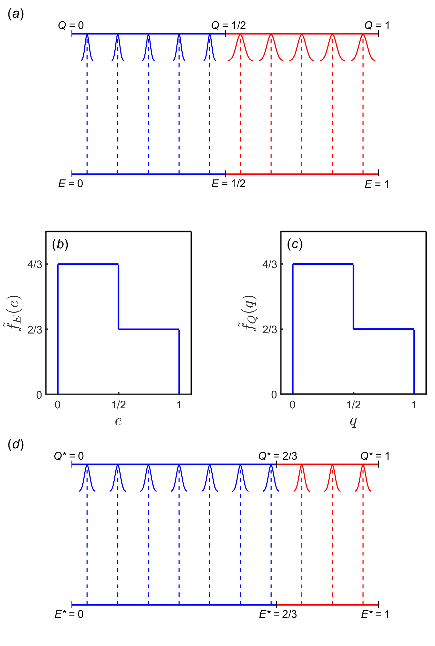
Figure 1: Transformation of variables when $\boldsymbol{h(Q|e)}$ varies with $\boldsymbol{e}$. This figure is calculated under the approximation of the slow-change regime. The figure applies for the special case $m(e)=e$, where the conditional distribution $f_{Q|E}(q|e)$ takes two different forms, depending on whether $e<1/2$ or $e\geq 1/2$. The two forms of $f_{Q|E}(q|e)$ are such that the entropy, $h(Q|e)$, for $e\geq 1/2$, exceeds the corresponding entropy for $e<1/2$ by an amount of unity. Panel (a): This panel contains dotted lines that connect values of $e$ with the associated values of $m(e)$. The bell-shaped curves represent conditional distributions of $Q$ (i.e., $f_{Q|E}(q|e)$) centered on various values of $m(e)$. Note that, here and in Fig. 2, these bell-shaped curves are illustrative, and are not drawn to scale. Panels (b&c): The marginal distributions $\tilde{f}_{E}(e)$ and $\tilde{f}_{Q}(q)$ are plotted for the situation described. Panel (d): This panel is the analogue of Panel (a) of this figure, after the transformations of Eqs. (7) and (8) have been applied. Note that as a consequence of the transformations, the scale has been stretched for $e<1/2$, and squeezed for $e\geq 1/2$. For example, when $q=1/2$, we have $q^{\ast}=2/3+O(\sigma_{\max})$. The same happens for $e$ and $e^{\ast}$. As a result, for all values of $e^{\ast}$, the mean of $f_{Q^{\ast}|E^{\ast}}(q^{\ast}|e^{\ast})$ equals $e^{\ast}+O(\sigma_{\max})$. In addition, the entropy of $f_{Q^{\ast}|E^{\ast}}(q^{\ast}|e^{\ast})$ has the same value for all values of $e^{\ast}$. In Panels (a) and (d), the parts shown in red relate to values of $e$ for which, before transformation, $h(Q|e)$ is relatively large.

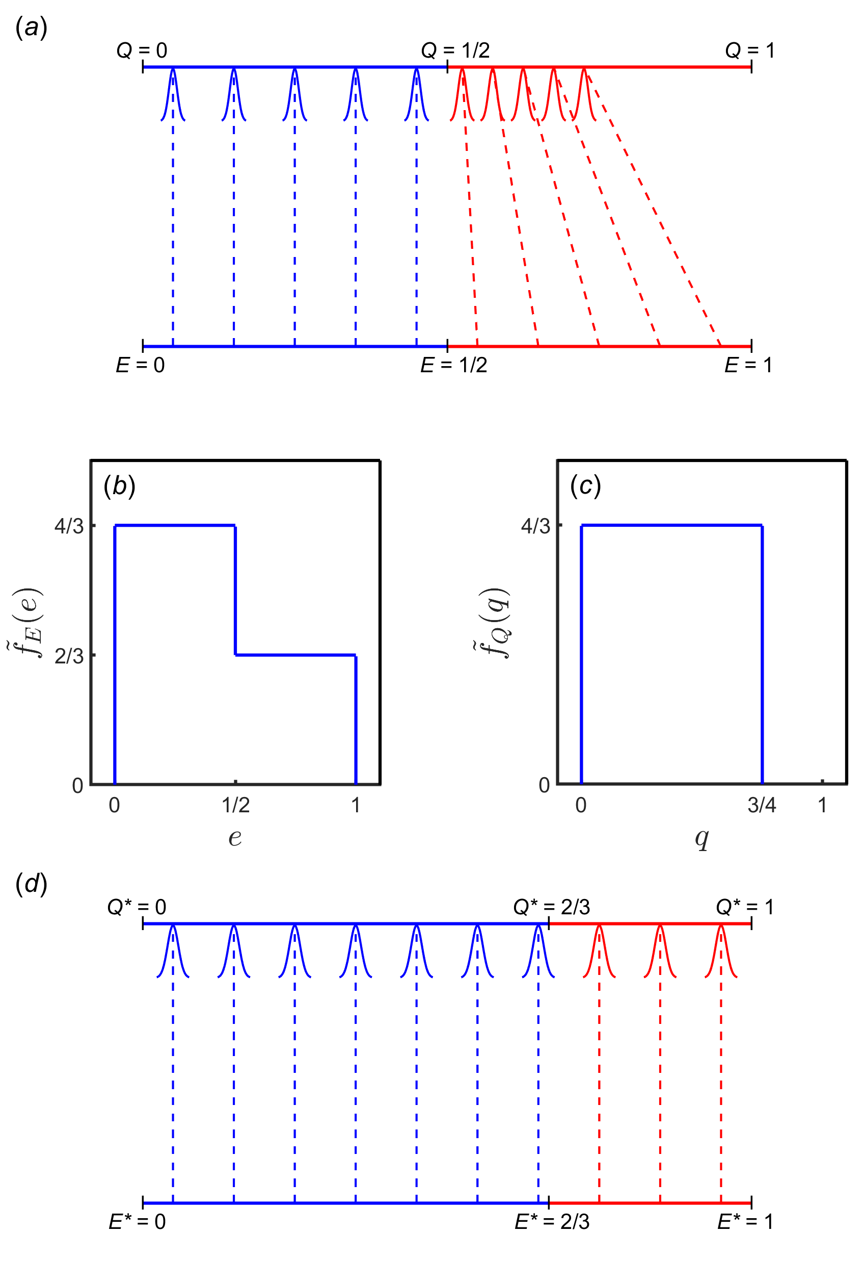
Figure 2: Transformation of variables when $\boldsymbol{m}^{\prime}\boldsymbol{(e)}$ varies with $\boldsymbol{e}$. This figure is calculated under the approximation of the slow-change regime. The figure applies for the special case where $m^{\prime}(e)=1$ for $e<1/2$, and $m^{\prime}(e)=1/2$ for $e\geq 1/2$. For this figure we assume that $h(Q|e)$ has the same value for all possible values of $e$. Panel (a): This panel contains dotted lines that connect values of $e$ with the associated values of $m(e)$. Panels (b&c):, The marginal distributions $\tilde{f}_{E}(e)$ and $\tilde{f}_{Q}(q)$ are plotted for the situation described. Panel (d): This panel is the analogue of Panel (a) of this figure, after the transformations of Eqs. (7) and (8) have been applied. The transformation from $E$ to $E^{\ast}$ is exactly as in Fig. 1. The transformation, from $Q$ to $Q^{\ast}$, involves a uniform stretching of the scale (by a factor of $4/3$) for $q<3/4$. Thus, when $q=1/2$ we have $q^{\ast}=2/3+O(\sigma_{\max})$, and when $q=3/4$ we have $q^{\ast}=1+O(\sigma_{\max})$. The differences in the way that $Q$ and $E$ are transformed result in an alignment such that, for all values of $e^{\ast}$, the mean of $f_{Q^{\ast}|E^{\ast}}(q^{\ast}|e^{\ast})$ is equal to $e^{\ast}+O(\sigma_{\max})$. In Panels (a) and (d), parts shown in red relate to values of $e$ for which, before transformation, $m^{\prime}(e)=1/2$.

Fig. 2 relates to the second source of statistical noise that can cause uncertainty about the state of the environment (i.e., about the value of $E$). This source is associated with the numerator of Eq. (10), and it arises when there is overlap in the conditional distributions of $Q$ that are associated with two different values of $E$. This overlap, in turn, depends on $m^{\prime}(e)$, the derivative, with respect to $e$, of the mean of the conditional distribution of $Q$. Indeed, if $m^{\prime}(e)$ is a constant for all values of $e$, then, for any two different values of $e$, the separation of the means of the two associated distributions of $Q$ vanishes in the limit as $m^{\prime}(e)\rightarrow 0$, and the overlap of the two distributions approaches zero in the limit as $m^{\prime}(e)\rightarrow\infty$.

In Fig. 2, the entropy associated with $f_{Q|E}(q|e)$ does not change as a function of $e$. However, for $e<1/2$ we have $m^{\prime}(e)=1$, while for $e\geq 1/2$ we have $m^{\prime}(e)=1/2$. This leads to the form of $\tilde{f}_{E}(e)$ shown in Fig. 2b, and thus to the form of $\tilde{f}_{Q}(q)$ shown in Fig. 2c. In the construction of $E^{\ast}$, the form of $\tilde{f}_{E}(e)$ leads to exactly the same stretching and shrinking of the distance between values of $E$ that was seen in Fig. 1. On the other hand, the form of $\tilde{f}_{Q}(q)$ leads, in the construction $Q^{\ast}$, to a uniform expansion of the space between values of $Q$. (This uniform expansion occurs for all values of $Q$ that are associated with a non-zero probability density.) As a result of these two different transformations, there is an alignment of the values of $E^{\ast}$ with the means of the associated conditional distributions of $Q^{\ast}$ values, as shown by the vertical dotted lines in Fig. 2d. Furthermore, the uniform expansion that creates $Q^{\ast}$ means that, for every possible environmental condition (i.e., for every possible value of $e^{\ast}$), the entropy of $Q^{\ast}$ increases and becomes equal (in absolute value) to the channel capacity.

Figure 3: Transformation of variables when the variance cannot be homogenized. In this case $f_{Q|E}(q|e)$ is assumed to take two different forms. For $e<3/5$ the form of $f_{Q|E}(q|e)$ is shown in Panel (a), while for $e\geq 3/5$ the form of $f_{Q|E}(q|e)$ is shown in Panel (b). Panels (c&d): The marginal distributions $\tilde{f}_{E}(e)$ and $\tilde{f}_{Q}(q)$ are plotted for the situation described. Panels (e&f): The two possible forms of the conditional distribution of the measuring variable ($Q^{\ast}$), namely $f_{Q^{\ast}|E^{\ast}}(q^{\ast}|e^{\ast})$, are plotted as functions of $q^{\ast}$.

In Fig. 1 the transformation that constructs $Q^{\ast}$ ensures that $h(Q^{\ast}|e^{\ast})$ is independent of $e^{\ast}$. This is accomplished by stretching and shrinking the space between various values of $Q$ in a way that may homogenize the variance of the conditional distributions of $Q^{\ast}$ that are associated with various values of $E^{\ast}$. However, it is of interest to consider what happens when such a homogenization of variance is not possible. A very simple example of such a situation is portrayed in Fig. 3. Here, we assume that only two forms of the conditional distribution of $Q$ are possible, and both forms have exactly the same mean. The first form of the conditional distribution of $Q$ is associated with values of $E$ that are less than $3/5$. This is a uniform distribution with mean equal to $1/2$ (see Fig. 3a). The second form of the conditional distribution of $Q$ is associated with values of $E$ that equal or exceed $3/5$. This second form of the conditional distribution also has a mean of $1/2$ and it is also uniform. However, its variance is four times that of the first form of the distribution (see Fig. 3b). In Appendix F we show that no increasing transformation (as defined above) can homogenize the variance such that, after the transformation, the variance for the two possible forms of the conditional distributions of the transformed measuring variable will be the same.

For this example, we picked $3/5$ as the critical value of $E$ because, when $E$ is uniformly distributed from $0$ to $1$, this results in the information-maximising distribution of $E$ (i.e., $\tilde{f}_{E}(e)$), which is shown in Fig. 3c. From this we can obtain $\tilde{f}_{Q}(q)$, as shown in Fig. 3d. Because $\tilde{f}_{E}(e)$ is uniform on the interval from $0$ to $1$, application of Eq. (7) has no effect, so that any distribution of values of $E$ is identical to the associated distribution of values of $E^{\ast}$ that is obtained from the transformation represented by Eq. (7).

In constructing $Q^{\ast}$, the form of $\tilde{f}_{Q}(q)$ leads to a uniform expansion of the distance between values of $Q$ for those values of $Q$ that lie between $1/4$ and $3/4$. For values of $Q$ that are above or below these limits, the form of $\tilde{f}_{Q}(q)$ leads to a shrinking of the distance between values of $Q$ when $Q^{\ast}$ is constructed. The result is the creation of two possible forms for the conditional distribution of $Q^{\ast}$ (i.e., $f_{E^{\ast}|Q^{\ast}}(e^{\ast}|q^{\ast})$). The first of these is associated with values of $e^{\ast}$ that are less than $3/5$, and this is shown in Fig. 3e. The second form is for values of $e^{\ast}$ that equal or exceed $3/5$, and is shown in Fig. 3f. Obviously, the variance of the distribution shown in Fig. 3e is less than that for the distribution in Fig. 3f. Nevertheless, the entropy of these two distributions is identical, as guaranteed by the analysis presented in Appendix F. This Appendix also provides a calculation to demonstrate that, in this case, if $E^{\ast}$ takes its uniform, information-maximising form, we nevertheless gain more information about the value of $E^{\ast}$ when we observe some values of $Q^{\ast}$ compared with other values. Note that, as mentioned above, this cannot happen under the slow-change regime.

III Explaining the results

Explicit proofs of the claims made in this work are contained in the Appendices. In this section we hope to give some insight into the mathematical realities that lie behind the results, and into the logic followed in the proofs that appear in the Appendices. We will focus on the core result, as embodied in Theorem 1. This theorem states that the entropy of $Q^{\ast}$ is independent of the nature of the environment in which the entropy of $Q^{\ast}$ is measured, namely $h(Q^{\ast}|e^{\ast})$).

Note that this section is quite technical, and some readers may prefer to skip directly to the Discussion, in which the possible wider implications of the results are discussed.

III-A Why is the entropy of $Q^{\ast}$ independent of environmental conditions?

It is reasonable to ask why the transformation specified by Eq. (8) leads to the homogenization of the entropy of the transformed measuring variable ($Q^{\ast}$) that is found under different environmental conditions. Here we will attempt, in a non-rigorous way, to provide some insight as to why this result is true.

For our current purposes, it is convenient to define the conditional entropy of $Q$ as the weighted average of $h(Q|e)$ over the values of $e$ that occur. We write this weighted average as $h(Q|E)$ and thus have $h(Q|E)=\int_{-\infty}^{\infty}h(Q|e)f_{E}(e)de$. This can be used to rewrite Eq. (3) as:

$$I(Q;E)=h(Q)-h(Q|E).$$ (16)

Recall that the channel capacity is the maximum-possible value of $I(Q;E)$. Channel capacity is achieved when the distribution of environmental effects ($f_{E}(e)$) takes on its information-maximising form, which we have called $\tilde{f}_{E}(e)$. Now, let us imagine that, for sufficiently small deviations in the distribution of environments from $\tilde{f}_{E}(e)$, the value of $h(Q)$ (i.e., the entropy of $Q$) is unchanged. If this was true, then what would it tell us about the entropy of $Q$ under various environmental conditions? That is, what would it tell us about the value of $h(Q|e)$ that we would find for various values of $e$?

The answer is that this odd set of circumstances would imply that there is no variation among the values of $h(Q|e)$. To see why, imagine, for example, that $\tilde{f}_{E}(e)$ is non-zero on the interval $(0,1)$, and that $h(Q|e)$ is smaller, for all allowed $e<0.2$, compared with $h(Q|e)$ for all allowed $e\geq 0.2$. In this case, if $f_{E}(e)$ takes its information-maximising form (i.e., $\tilde{f}_{E}(e)$), then we could decrease $h(Q|E)$ by increasing $f_{E}(e)$ for $e<0.2$, while simultaneously decreasing $f_{E}(e)$ for $e\geq 0.2$. Note that, by our assumption, a sufficiently small change in $f_{E}(e)$ from $\tilde{f}_{E}(e)$ will not alter $h(Q)$, and so this decrease in $h(Q|E)$ (if the associated change in $f_{E}(e)$ is sufficiently small) will lead to an increase in the mutual information, $I(Q;E)$ (Eq. (16)). However, this increase in $I(Q;E)$ is impossible because it arose by changing $f_{E}(e)$ from $\tilde{f}_{E}(e)$, and $\tilde{f}_{E}(e)$ is defined as the information-maximising form of $f_{E}(e)$. This logical contradiction shows that our initial assumptions are incompatible. In other words, if our assumption that $h(Q)$ is unchanged by sufficiently small changes in $f_{E}(e)$ from $\tilde{f}_{E}(e)$ is true, then variation in $h(Q|e)$ of the sort described must be impossible. By extending this example to all possible cases of variation in the $h(Q|e)$ values, we can show that, in general, the assumption about the immutability of $h(Q)$ when $f_{E}(e)$ is sufficiently close to $\tilde{f}_{E}(e)$ implies that no variation is possible among the values of $h(Q|e)$ that are associated with the various possible values of $e$.

Of course, in general, $h(Q)$ will not be unaffected by changes in $f_{E}(e)$ when $f_{E}(e)$ is similar to $\tilde{f}_{E}(e)$, and thus variation in $h(Q|e)$ is possible. However, consider what would happen if, when $f_{E}(e)$ takes its information-maximising form (namely $\tilde{f}_{E}(e)$), it so happened that the resulting distribution of $Q$ (i.e., $\tilde{f}_{Q}(q)$) was uniform on some interval (and had zero height elsewhere).

As noted above, a uniform distribution maximises the entropy (in comparison with all other distributions that have non-zero probability density only on a particular interval). A direct implication of this maximisation is that very small changes in non-zero values of ${f}_{Q}(q)$ lead to yet smaller effects on $h(Q)$. In particular, if the deviation of ${f}_{Q}(q)$ is of order $\alpha$, then the changes to $h(Q)$ will be of order $\alpha^{2}$.

Of course, changes in $h(Q)$ that are of order $\alpha^{2}$ are not the same as no change at all to $h(Q)$. However, because $\alpha^{2}$ vanishes in comparison to $\alpha$ as $\alpha$ approaches zero, it turns out that these changes in $h(Q)$ are small enough to force equality among the values of $h(Q|e)$ that obtain for different values of $e$. However, this equality depends on our supposition that $\tilde{f}_{Q}(q)$ is uniform. In general, it will not be uniform. However, we can use an increasing transformation to create a new variable with a different distribution. A function that does this in a way that ensures that the new distribution is uniformly distributed on the interval $(0,1)$ is given by Eq. (8). Thus, for the transformed variable produced by Eq. (8) (namely $Q^{\ast}$), it is plausible that the entropy (namely $h(Q^{\ast}|e)$) must be equal for all possible values of $e$.

III-B Summary of the proof that the entropy of $Q^{\ast}$ is independent of environmental conditions

We shall now provide a sketch of the proof, contained in Appendices C and D, that demonstrates the independence of the entropy of $Q^{\ast}$ from the value of $e^{\ast}$ (which is a measure of environmental conditions). These results arise, in part, from the condition that the mutual information is maximised. To find this condition, we look for the form of the distribution of $E$, such that to linear order in changes in this distribution, the mutual information does not change (in a functional sense, independence of changes, at linear order, is a basic condition for stationarity). The form of the distribution of $E$ that maximises the mutual information is written as $\tilde{f}_{E}(e)$. We find it satisfies

$$\int_{-\infty}^{\infty}f_{Q|E}(q|e)\log_{2}\left[\tilde{f}_{Q}(q)\right]dq+h(Q|e)=-\widetilde{I}(Q;E)$$ (17)

with $\tilde{f}_{E}(e)$ implicitly present because of its control over the form of $\tilde{f}_{Q}(q)$ (see Eq. (6)). The freedom that arises from the mutual information being unchanged in value, when the random variables $Q$ and $E$ are replaced by new random variables that are increasing transformations of $Q$ and $E$, allows us to transform the left side of Eq. (17), without changing the value of $\widetilde{I}(Q;E)$. In particular, when the distribution of $E$ maximises the mutual information, it is possible to find an increasing transformation that converts $Q$ to a new random variable, $Q^{\ast}$, with the special property that its distribution, $\tilde{f}_{Q^{\ast}}(q^{\ast})$, is uniform over $0<q^{\ast}<1$ and zero elsewhere. When we use $Q^{\ast}$ in place of $Q$ in Eq. (17), we note that the first term on the left hand side of this equation vanishes identically ($\log_{2}\left[1\right]=0$) and we arrive at $h(Q^{\ast}|e)=-\widetilde{I}(Q;E)$. This result indicates that the entropy $h(Q^{\ast}|e)$ has been homogenized in the sense that it is independent of the value of $e$. Additionally, we are still free to transform $E$. It is also possible to find an increasing transformation that converts $E$ to a new random variable $E^{\ast}$ that is uniform over $0<e^{\ast}<1$ and zero elsewhere. This leads to the result $h(Q^{\ast}|e^{\ast})=-I_{\max}(Q;E)$ and indicates that the entropy $h(Q^{\ast}|e^{\ast})$ is independent of $e^{\ast}$ for $0<e^{\ast}<1$.

IV Discussion

As we have seen, transformations of the sort described by Eqs. (7) and (8) do not change the amount of information that knowledge about one variable provides about the state of another variable. With that in mind, it is worth considering whether such transformations can be of any practical use.

Under certain conditions, the transformations described by Eqs. (7) and (8) make natural relationships behave in a manner that is similar to the relationship between a continuously varying environmental variable and a typical measuring device that is behaving properly. The fact that humans go to so much trouble to produce good measuring devices suggests that, in itself, this effect of the transformations is valuable. They bring a certain homogeneity in that, after they are applied, the effect of the environmental variable on the measuring variable can be about the same throughout the range of possible environmental-variable values. Humans apparently find this sort of homogeneity to be pleasing and/or useful.

A very practical possible application of the results presented here has to do with statistical analysis. For data sets that arise from causal relationships that are sufficiently similar to the situation described by the slow-change regime, the methods described here can transform the data so as to linearise the relationship between two data sets, and to homogenize the entropy among samples collected under different conditions. As entropy is often closely related to variance, this may imply a homogenization of variance as well. Regression analysis and similar techniques often assume a linear relationship between independent and dependent variables, and they also typically assume that the variance is homogeneous. Thus, the transformations described here may be useful in adjusting data so as to meet the requirements for the most powerful statistical techniques available for data analysis [9]. Even for situations that are very different from those described by the slow-change regime, a transformation of the sort described here can typically be used to homogenize the entropy of $Q$, the measuring variable, and it seems likely that this will be advantageous when statistical analyses are carried out.

Given that the transformations described here homogenize entropy in measuring variables (which may or may not have implications for the homogenization of the variance) it is interesting to speculate on the possibility of developing hypothesis-testing analyses in which the measure of data dispersion is entropy, and not the variance ([10], [11], [12]). This possibility is particularly intriguing because there are situations in which entropy can be homogenized, but variance cannot. (A simple example is provided in Fig. 3.) In this regard, the transformations bear some resemblance to histogram equalisation, which is a method employed to enhance low-quality optical images, amongst other uses ([13], [14], [15], [16]). However, this resemblance is in appearance only, since histogram equalisation does not generally lead to a homogenization of entropy between environmental conditions. This is due, in part, to the fact that, unlike the transformations we have described in the present study, histogram equalisation does not involve using the information- maximising distribution of the causal variable to create a transformed version of the caused variable. Instead, in histogram equalisation, the distribution of inputs (the causal variable) is typically taken from real-world data. For example, to use histogram equalisation to enhance a digital image of a countryside scene, one might use the distribution of brightness levels that are reflected from objects in a natural landscape.

In this work we have focused on the information-theoretic analysis of continuous variables. However, discrete variables have generally attracted much more attention from information theorists than have continuous variables. It is not obvious how to apply some of the concepts that have been developed in the realm of discrete variables to the case of continuous variables. One example of this difficulty has to do with the concept of functional information, as proposed by J. Szostak ([17], [18]). Szostak, writing in the context of biomolecules such as enzymes, says that “functional information is simply $-\log_{2}$ of the probability that a random sequence will encode a molecule with greater than any given degree of function” [17]. In addition to its use in the context of biomolecules, functional information (or a very similar concept) has also been used to characterise adaptation [1] and the closely allied concept of ‘biological complexity’ ([19], [20]). In these cases, expected reproductive success (i.e., fitness) is the ‘function’ in terms of which the functional information associated with different types of organisms is evaluated. However, these wider applications have been confined to studying the adaptedness of genomes (or the biological complexity of genomes). This is problematic because it is in the realm of phenotypes that adaptedness is generally recognised. We infer a highly adapted genotype when we see a highly adapted phenotype, and, in general, not vice versa. Thus, it would be advantageous to be able to apply the idea of functional information to the continuously varying traits that are typically used to characterise phenotypes.

Unfortunately, the value of functional information for a continuously varying phenotypic variable will, in general, depend on how that variable is transformed. For example, if the variable is body mass, then we might measure the fitness associated with different body-mass values (holding all else constant), and thus we could calculate the functional information associated with any given body mass. However, we may get very different values for functional information if, instead of body mass, we consider the logarithm of body mass. This would introduce problematic ambiguity if there was no natural transformed variable with which to measure body mass. However, the variation in body mass that we see within groups of organisms tends to relate, in part, to the different evolutionary pressures that prevail in various environments ([21], [22], [23]). This relationship might usefully be characterised as a causal relationship of the sort discussed above. As such, the results presented here suggest that, typically, there will be a natural transformed variable to use in the measurement of body mass (or whatever other continuously varying trait is being considered). This, in turn, suggests that the results presented here may facilitate the extension of information-theoretic concepts that were developed in the context of discrete variables to the realm of continuously distributed variables. The implications of the resulting increase in analytic power are not clear, but they may include the development of useful quantitative tools to study some of the most fascinating phenomena that are associated with life.

Acknowledgements

It is a pleasure to thank Antonio Carvajal Rodriguez, Yuval Simons, and John Welch for helpful discussions during the preparation of this study, and Professor C. Adami, Professor O. Johnson and an anonymous reviewer for very helpful comments on our manuscript.

APPENDICES

In the following appendices, when we refer to a particular distribution we mean a particular ‘probability density function’, and when we refer to an entropy, we mean the ‘differential entropy’ (which is the entropy associated with a continuous random variable [3]).

We shall also make use of the Dirac delta function which, for argument $x$, is written $\delta(x)$. The Dirac delta function, $\delta(x)$, is a spike-like probability density, with a vanishingly small variance and an area of unity that is located at $x=0$. We shall freely exploit the following two properties of a Dirac delta function: (i) with $\mathbb{E}\left[...\right]$ denoting an expected value, the joint probability density function of two random variables $E$ and $Q$, when evaluated at the values $e$ and $q$, respectively, is $\mathbb{E}\left[\delta\left(e-E\right)\delta\left(q-Q\right)\right]$ (see e.g., the textbook [24] for this point of view); (ii) when a function of $x$, say $q(x)$, vanishes at only one point, say $x_{0}$, the quantity $\delta(q(x))$ equals $\delta(x-x_{0})/|q^{\prime}(x_{0})|$ where $q^{\prime}(x)=dq(x)/dx$ (see e.g., [25]).

Appendix A Mathematical details of the model

In this appendix we introduce the form of the joint distribution of the random variables $Q$ and $E$ that we consider in this work. The joint distribution of $Q$ and $E$ arises from a fixed form of the conditional distribution, $f_{Q|E}(q|e)$, but different forms of the marginal distribution of $E$, namely $f_{E}(e)$.

This appendix also contains basic mathematical details of the model adopted, along with definitions of some key distributions and the mutual information.

To begin, consider a mathematical model involving two continuous one-dimensional random variables that we write as $E$ and $Q$. Generally, $E$ and $Q$ are not statistically independent.

We shall write the limits of various integrals involving distributions of the random variables $E$ and $Q$ as ranging from $-\infty$ to $\infty$, implicitly assuming that possible values of $E$ and $Q$ lie in this infinite range. However, when we consider new random variables (related to $E$ and $Q$) that take values in a smaller range, the corresponding distributions will vanish outside the ranges of the new variables, and make no contribution to the integrals. When we need to be explicit about finite ranges of random variables, we will indicate this in the limits of any integrals that arise.

A-A Distributions

Some properties of important distributions are as follows.

1. The conditional distribution of $Q$, given that $E$ takes the value $e$ (i.e., given that $E=e$), is written as $f_{Q|E}(q|e)$. This, like all probability density functions, has a total integrated probability of unity, and for the present case this reads

   $$\int_{-\infty}^{\infty}f_{Q|E}(q|e)dq=1.$$ (18)

   A key assumption of this work is that $f_{Q|E}(q|e)$ has its $q$ and $e$ dependence specified at the outset, and its specified form is not varied in the ensuing analysis. By contrast, we shall consider different forms of the marginal distribution of $E$, written $f_{E}(e)$.

2. The joint distribution of $Q$ and $E$ is given in terms of $f_{Q|E}(q|e)$ and $f_{E}(e)$ as

   $$f_{Q,E}(q,e)=f_{Q|E}(q|e)f_{E}(e).$$ (19)

3. The marginal distribution of $Q$ is given by

   $$f_{Q}(q)=\int_{-\infty}^{\infty}f_{Q|E}(q|e)f_{E}(e)de.$$ (20)

We note that because of the fixed nature of $f_{Q|E}(q|e)$, different forms of $f_{E}(e)$ produce different statistical properties of both $E$ and $Q$. In particular, Eqs. (19) and (20) explicitly show that the distributions $f_{Q,E}(q,e)$ and $f_{Q}(q)$ depend on the marginal distribution of $E$, namely $f_{E}(e)$. As a consequence, a change in $f_{E}(e)$ induces changes in both $f_{Q,E}(q,e)$ and $f_{Q}(q)$.

A-B Differential entropy and mutual information

A continuous random variable, such as $Q$, has an entropy (strictly, differential entropy) that we denote by $h(Q)$, and is defined by

$$h(Q)=-\int_{-\infty}^{\infty}f_{Q}(q)\log_{2}\left[f_{Q}(q)\right]dq$$ (21)

where $\log_{2}\left(x\right)$ denotes the logarithm of $x$ to base $2$.

Let us suppose that the random variable $E$ is observed to take the particular value $e$ (i.e., $E=e$). Then the relevant distribution of $Q$ is the conditional probability density of $Q$, given that $E=e$, namely $f_{Q|E}(q|e)$. The entropy associated with $Q$ in this case is written as $h(Q|e)$, and is calculated from $f_{Q|E}(q|e)$ according to

$$h(Q|e)=-\int_{-\infty}^{\infty}f_{Q|E}(q|e)\log_{2}\left[f_{Q|E}(q|e)\right]dq.$$ (22)

The mutual information is defined as

$$I(Q;E) =\int_{-\infty}^{\infty}\left[h(Q)-h(Q|e)\right]f_{E}(e)de$$

$$=h(Q)-\int_{-\infty}^{\infty}h(Q|e)f_{E}(e)de.$$ (23)

This is closely analogous to the mutual information of a pair of discrete random variables, which corresponds to the average reduction in the uncertainty of $Q$ that results from knowledge of the value of $E$.

Appendix B Increasing transformations

In this appendix we demonstrate that the value of the mutual information is unchanged on replacing the random variables $Q$ and $E$ by independent (and generally different) transformations of these random variables. The transformations are implemented with functions that are at least once differentiable and strictly increasing and in this work are termed increasing transformations.

In Appendix A, we started with the random variables $Q$ and $E$. We now consider transformed versions of these variables. Using transformed versions of $Q$ and $E$ gives us the freedom to make different choices of the transformations adopted.

To define the transformed variables, we introduce two real functions, $P(x)$ and $D(x)$, that are at least once differentiable and are strictly increasing. We shall call such functions ‘increasing transformations’. We then define a pair of new continuous random variables, $Q^{\circ}$ and $E^{\circ}$ via

$$Q^{\circ}=P(Q)$$ (24)

and

$$E^{\circ}=D(E)$$ (25)

which are thus increasing transformations of the random variables $Q$ and $E$, respectively. Note that Eq. (24) is equivalent to $q^{\circ}=P(q)$, where $q$ is a particular value of $Q$ and $q^{\circ}$ is the corresponding particular value of $Q^{\circ}$ that arises. Similarly, Eq. (25) is equivalent to $e^{\circ}=P(e)$, where $e$ is a particular value of $E$ and $e^{\circ}$ is the corresponding particular value of $E^{\circ}$ that arises.

Increasing transformations are invertible, which means, for example, that $Q^{\circ}$ uniquely determines $Q$ and vice versa. Thus Eqs. (24) and (25) can also be written as $Q=P^{(-1)}(Q^{\circ})$ and $E=D^{(-1)}(E^{\circ})$ where a $(-1)$ superscript denotes the inverse function, such that $P(P^{(-1)}(x))=x$ and $P^{(-1)}(P(x))=x$.

It might be expected that $Q^{\circ}$ and $E^{\circ}$ are, in some sense, an equivalent way of describing the problem at hand. Indeed, we shall show that the mutual information between $Q$ and $E$, is identical to the mutual information between $Q^{\circ}$ and $E^{\circ}$. Thus, at the level of mutual information, the transformed pair of variables, $Q^{\circ}$ and $E^{\circ}$, are completely equivalent to the original pair of variables, $Q$ and $E$. Of course some versions of $Q^{\circ}$ and $E^{\circ}$ may have some additional properties that make them more useful than others.

We next show how some key statistical properties of the transformed variables ($Q^{\circ}$ and $E^{\circ}$) are related to the corresponding properties of the original variables ($Q$ and $E$). Since, in general, $Q^{\circ}$ and $E^{\circ}$ do not take the same range of values as the original variables, we shall incorporate this into the analysis by taking $Q^{\circ}$ to lie in the range $q_{1}^{\circ}$ to $q_{2}^{\circ}$, and $E^{\circ}$ to lie in the range $e_{1}^{\circ}$ to $e_{2}^{\circ}$.

B-A Conditional distributions $f_{Q^{\circ}|E^{\circ}}(q^{\circ}|e^{\circ})$ and $f_{E^{\circ}|Q^{\circ}}(e^{\circ}|q^{\circ})$

We stated in Appendix A that the conditional distribution $f_{Q|E}(q|e)$ is specified from the outset. It is convenient, however, to represent it in a form where it can be related to the corresponding distribution involving the transformed variables $Q^{\circ}$ and $E^{\circ}$. With $\mathbb{E}\left[...\right]$ denoting an expected value over $Q$ and $E$, and $\delta(x)$ denoting a Dirac delta function of argument $x$, the required representation of $f_{Q|E}(q|e)$ is given by

$$f_{Q|E}(q|e)=\frac{\mathbb{E}\left[\delta\left(q-Q\right)\delta(e-E)\right]}{\mathbb{E}\left[\delta(e-E)\right]}.$$ (26)

Consider now the corresponding conditional distribution of $Q^{\circ}$, conditional on the value of $E^{\circ}$, when evaluated at $q^{\circ}$ and $e^{\circ}$, respectively, namely $f_{Q^{\circ}|E^{\circ}}(q^{\circ}|e^{\circ})$. This can be similarly written as

$$f_{Q^{\circ}|E^{\circ}}(q^{\circ}|e^{\circ}) =\frac{\mathbb{E}\left[\delta\left(q^{\circ}-Q^{\circ}\right)\delta(e^{\circ}-E^{\circ}\right]}{\mathbb{E}\left[\delta(e^{\circ}-E^{\circ}\right]}$$

$$=\frac{\mathbb{E}\left[\delta\left(q^{\circ}-P(Q)\right)\delta(e^{\circ}-D(E))\right]}{\mathbb{E}\left[\delta(e^{\circ}-D(E))\right]}.$$ (27)

This is well defined for $e_{1}^{\circ}<e^{\circ}<e_{2}^{\circ}$ and in this range we have

$$f_{Q^{\circ}|E^{\circ}}(q^{\circ}|e^{\circ})$$

$$=\left\{\begin{array}[c]{ll}\tfrac{\mathbb{E}\left[\delta\left(P^{(-1)}(q^{\circ})-Q\right)\delta(D^{(-1)}(e^{\circ})-E)\right]}{P^{\prime}(P^{(-1)}(q^{\circ}))\mathbb{E}\left[\delta(D^{(-1)}(e^{\circ})-E)\right]}&\text{for }q_{1}^{\circ}<q^{\circ}<q_{2}^{\circ}\\ &\\ 0&\text{otherwise.}\end{array}\right.$$ (31)

This can then be directly expressed in terms of $f_{Q|E}(q|e)$, using Eq. (26), as

$$f_{Q^{\circ}|E^{\circ}}(q^{\circ}|e^{\circ})$$

$$=\left\{\begin{array}[c]{lll}\tfrac{f_{Q|E}(P^{(-1)}(q^{\circ})|D^{(-1)}(e^{\circ}))}{P^{\prime}(P^{(-1)}(q^{\circ}))}&&\text{for }q_{1}^{\circ}<q^{\circ}<q_{2}^{\circ}\\ &&\\ 0&&\text{otherwise.}\end{array}\right.$$ (36)

In a similar way the distribution $f_{E^{\circ}|Q^{\circ}}(e^{\circ}|q^{\circ})$ is well defined for $q_{1}^{\circ}<q^{\circ}<q_{2}^{\circ}$ and in this range is given by

$$f_{E^{\circ}|Q^{\circ}}(e^{\circ}|q^{\circ})$$

$$=\left\{\begin{array}[c]{lll}\tfrac{f_{E|Q}(D^{(-1)}(e^{\circ})|P^{(-1)}(q^{\circ}))}{D^{\prime}(D^{(-1)}(e^{\circ}))}&&\text{for }e_{1}^{\circ}<e^{\circ}<e_{2}^{\circ}\\ &&\\ 0&&\text{otherwise.}\end{array}\right.$$ (41)

B-B Marginal distributions $f_{E^{\circ}}(e^{\circ})$ and $f_{Q^{\circ}}(q^{\circ})$

The marginal distribution of $E$, when evaluated at $e$, can be written as $f_{E}(e)=\mathbb{E}\left[\delta(e-E)\right]$. The marginal distribution of $E^{\circ}$, when evaluated at $e^{\circ}$, is given by

$$f_{E^{\circ}}(e^{\circ})=\mathbb{E}\left[\delta(e^{\circ}-E^{\circ})\right]=\mathbb{E}\left[\delta(e^{\circ}-D(E))\right].$$ (43)

Since $E^{\circ}$ only takes values in the range $e_{1}^{\circ}$ to $e_{2}^{\circ}$ we have

$$f_{E^{\circ}}(e^{\circ})=\left\{\begin{array}[c]{lll}\dfrac{\mathbb{E}\left[\delta(D^{(-1)}(e^{\circ})-E)\right]}{D^{\prime}(D^{(-1)}(e^{\circ}))}&&\text{for }e_{1}^{\circ}<e^{\circ}<e_{2}^{\circ}\\ &&\\ 0&&\text{otherwise.}\end{array}\right.$$ (44)

This can be written as

$$f_{E^{\circ}}(e^{\circ})=\left\{\begin{array}[c]{lll}\dfrac{f_{E}(D^{(-1)}(e^{\circ})))}{D^{\prime}(D^{(-1)}(e^{\circ}))}&&\text{for }e_{1}^{\circ}<e^{\circ}<e_{2}^{\circ}\\ &&\\ 0&&\text{otherwise.}\end{array}\right.$$ (45)

Similarly, the marginal distribution of $Q^{\circ}$, when evaluated at $q^{\circ}$, is given by

$$f_{Q^{\circ}}(q^{\circ})=\left\{\begin{array}[c]{lll}\dfrac{f_{Q}(P^{(-1)}(q^{\circ}))}{P^{\prime}(P^{(-1)}(q^{\circ}))}&&\text{for }q_{1}^{\circ}<q^{\circ}<q_{2}^{\circ}\\ &&\\ 0&&\text{otherwise.}\end{array}\right.$$ (46)

B-C Differential entropy $h(Q^{\circ})$

We write the (differential) entropy of $Q$ as $h(Q)$. This is given in Eq. (21). The corresponding entropy of $Q^{\circ}$ is written as $h(Q^{\circ})$ and given by $h(Q^{\circ})=-\int_{q_{1}^{\circ}}^{q_{2}^{\circ}}f_{Q^{\circ}}(q^{\circ})\log_{2}\left[f_{Q^{\circ}}(q^{\circ})\right]dq^{\circ}$. Using Eq. (46) yields
$h(Q^{\circ})=-\int_{q_{1}^{\circ}}^{q_{2}^{\circ}}\frac{f_{Q}(P^{(-1)}(q^{\circ}))}{P^{\prime}(P^{(-1)}(q^{\circ}))}\log_{2}\left[\frac{f_{Q}(P^{(-1)}(q^{\circ}))}{P^{\prime}(P^{(-1)}(q^{\circ}))}\right]dq^{\circ}$ and with the change of variables $q^{\circ}=P(q)$ we obtain

$$h(Q^{\circ}) =-\int_{-\infty}^{\infty}f_{Q}(q)\log_{2}\left[\frac{f_{Q}(q)}{P^{\prime}(q)}\right]dq$$

$$=h(Q)+\int_{-\infty}^{\infty}f_{Q}(q)\log_{2}\left[P^{\prime}(q)\right]dq.$$ (47)

B-D Differential entropy $h(Q^{\circ}|e^{\circ})$

We write the entropy of $Q$, when $E$ takes the particular value $e$, as $h(Q|e)$. This is given in Eq. (22). We write the corresponding entropy of $Q^{\circ}$, given that $E^{\circ}$ takes the particular value $e^{\circ}$, as $h(Q^{\circ}|e^{\circ})$ and this is given by

$$h(Q^{\circ}|e^{\circ}) =-\int_{q_{1}^{\circ}}^{q_{2}^{\circ}}f_{Q^{\circ}|E^{\circ}}(q^{\circ}|e^{\circ})\log_{2}\left[f_{Q^{\circ}|E^{\circ}}(q^{\circ}|e^{\circ})\right]dq^{\circ}$$

$$=-\int_{q_{1}^{\circ}}^{q_{2}^{\circ}}\frac{f_{Q|E}(P^{(-1)}(q^{\circ})|D^{(-1)}(e^{\circ}))}{P^{\prime}(P^{(-1)}(q^{\circ}))}$$

$$\quad\times\log_{2}\left[\frac{f_{Q|E}(P^{(-1)}(q^{\circ})|D^{(-1)}(e^{\circ}))}{P^{\prime}(P^{(-1)}(q^{\circ}))}\right]dq^{\circ}$$

$$=-\int_{-\infty}^{\infty}f_{Q|E}(q|D^{(-1)}(e^{\circ}))$$

$$\quad\times\log_{2}\left[\frac{f_{Q|E}(q|D^{(-1)}(e^{\circ}))}{P^{\prime}(q)}\right]dq$$

$$=h(Q|D^{(-1)}(e^{\circ}))$$

$$\quad+\int_{-\infty}^{\infty}f_{Q|E}(q|D^{(-1)}(e^{\circ}))\log_{2}\left[P^{\prime}(q)\right]dq.$$ (48)

B-E Mutual information $I(Q^{\circ};E^{\circ})$

The mutual information about $Q{\tiny\ }$that is gained from knowledge of $E$ is written $I(Q;E)$ and is given in Eq. (23). The corresponding mutual information that we gain about the value of $Q^{\circ}$, from knowledge of $E^{\circ}$, is written as $I(Q^{\circ};E^{\circ})$ and given by

$$I(Q^{\circ};E^{\circ})=\int_{e_{1}^{\circ}}^{e_{2}^{\circ}}\left[h(Q^{\circ})-h(Q^{\circ}|e^{\circ})\right]f_{E^{\circ}}(e^{\circ})de^{\circ}.$$ (49)

We have, using above results for $h(Q^{\circ})$ and $h(Q^{\circ}|e^{\circ})$, that

$$h(Q^{\circ})-h(Q^{\circ}|e^{\circ})$$

$$=h(Q)-h(Q|D^{(-1)}(e^{\circ}))$$

$$+\int_{-\infty}^{\infty}\left[f_{Q}(q)-f_{Q|E}(q|D^{(-1)}(e^{\circ}))\right]\log_{2}\left[P^{\prime}(q)\right]dq.$$ (50)

Thus

$$I(Q^{\circ};E^{\circ})$$

$$=\int_{e_{1}^{\circ}}^{e_{2}^{\circ}}\left[h(Q^{\circ})-h(Q^{\circ}|e^{\circ})\right]f_{E^{\circ}}(e^{\circ})de^{\circ}$$

$$=\int_{e_{1}^{\circ}}^{e_{2}^{\circ}}\left[h(Q)-h(Q|D^{(-1)}(e^{\circ}))\right]\frac{f_{E}(D^{(-1)}(e^{\circ}))}{D^{\prime}(D^{(-1)}(e^{\circ}))}de^{\circ}$$

$$\quad+\int_{-\infty}^{\infty}dq\int_{e_{1}^{\circ}}^{e_{2}^{\circ}}de^{\circ}\left[f_{Q}(q)-f_{Q|E}(q|D^{(-1)}(e^{\circ}))\right]$$

$$\quad\times\log_{2}\left[P^{\prime}(q)\right]\frac{f_{E}(D^{(-1)}(e^{\circ}))}{D^{\prime}(D^{(-1)}(e^{\circ}))}.$$ (51)

The second integral in the above expression vanishes identically, hence $I(Q^{\circ};E^{\circ})=\int_{-\infty}^{\infty}\left[h(Q)-h(Q|e)\right]f_{E}(e)de$ or

$$I(Q^{\circ};E^{\circ})=I(Q;E).$$ (52)

It follows that when $Q^{\circ}$ is related to $Q$ by an increasing transformation, and $E^{\circ}$ is related to $E$ by a generally different increasing transformation (as given in Eqs. (24) and (25), respectively), the mutual information between $Q^{\circ}$ and $E^{\circ}$ is identical to the mutual information between $Q$ and $E$.

Appendix C Maximum mutual information

In this appendix, we vary the distribution $f_{E}(e)$ and determine a condition that the mutual information is maximal. This condition implicitly determines the form of $f_{E}(e)$ that maximises the mutual information. We write the maximising form of the distribution of $E$ as $\tilde{f}_{E}(e)$. From (1) it follows that the corresponding distribution of $Q$, when the mutual information is maximised, is $\tilde{f}_{Q}(q)=\int f_{Q|E}(q|e)\tilde{f}_{E}(e)de$.

The rationale of the calculations in this appendix are as follows: (i) the mutual information is a functional of the distribution of $E$, thus to determine the maximum mutual information, we perform a functional change in the distribution of $E$, such that the distribution always lies within the space non-negative functions that have a total integral of unity; (ii) we look for the condition that the mutual information does not change, to linear order in the functional change of the distribution of $E$. This is the condition for the maximum mutual information, and leads to an equation that determines the maximising distribution of $E$ and the channel capacity.

We begin, noting that in Appendix B it was shown that the mutual information between $Q$ and $E$ is identical to the mutual information between $Q^{\circ}$ and $E^{\circ}$. The mutual information can thus be maximised when expressed in terms of distributions of $Q$ and $E$, or in terms of distributions of $Q^{\circ}$ and $E^{\circ}$. We shall carry out the calculations in terms of the distributions of $Q^{\circ}$ and $E^{\circ}$, since this is an efficient way of obtaining all of the results we require.

We rewrite the form of the mutual information in Eq. (49) as

$$I(Q^{\circ};E^{\circ})$$

$$=\int_{q_{1}^{\circ}}^{q_{2}^{\circ}}\int_{e_{1}^{\circ}}^{e_{2}^{\circ}}f_{Q^{\circ}|E^{\circ}}(q^{\circ}|e^{\circ})\left\{\log_{2}\left[f_{Q^{\circ}|E^{\circ}}(q^{\circ}|e^{\circ})\right]\right.$$

$$\quad\left.-\log_{2}\left[f_{Q^{\circ}}(q^{\circ})\right]\right\}f_{E^{\circ}}(e^{\circ})dq^{\circ}de^{\circ}.$$ (53)

The above expression for $I(Q^{\circ};E^{\circ})$ depends on the form of the distribution $f_{E^{\circ}}(e^{\circ})$ (which by Eq. (45) is determined from the form of $f_{E}(e)$). We proceed by determining how $I(Q^{\circ};E^{\circ})$ behaves under the functional change of $f_{E^{\circ}}(e^{\circ})$ given by

$$f_{E^{\circ}}(e^{\circ})\rightarrow f_{E^{\circ}}(e^{\circ})+\Delta f_{E^{\circ}}(e^{\circ})$$ (54)

Let $\Delta f_{Q^{\circ}}(q^{\circ})$ denote the change in $f_{Q^{\circ}}(q^{\circ})$ that is produced by the change of $\Delta f_{E^{\circ}}(e^{\circ})$ in $f_{E^{\circ}}(e^{\circ})$. The transformed version of Eq. (20) is $f_{Q^{\circ}}(q^{\circ})=\int_{e_{1}^{\circ}}^{e_{2}^{\circ}}f_{Q^{\circ}|E^{\circ}}(q^{\circ}|e^{\circ})f_{E^{\circ}}(e^{\circ})de^{\circ}$ and hence

$$\Delta f_{Q^{\circ}}(q^{\circ})=\int_{e_{1}^{\circ}}^{e_{2}^{\circ}}f_{Q^{\circ}|E^{\circ}}(q^{\circ}|e^{\circ})\Delta f_{E^{\circ}}(e^{\circ})de^{\circ}.$$ (55)

This result indicates that $\Delta f_{Q^{\circ}}(q^{\circ})$ depends linearly on $\Delta f_{E^{\circ}}(e^{\circ})$.

We define $\Delta I(Q^{\circ};E^{\circ})$ to be the change in the mutual information, produced by the change of $\Delta f_{E^{\circ}}(e^{\circ})$ in $f_{E^{\circ}}(e^{\circ})$, to precisely first order in $\Delta f_{E^{\circ}}(e^{\circ})$, while the change in $I(Q^{\circ};E^{\circ})$ to second order in $\Delta f_{E^{\circ}}(e^{\circ})$ indicates that the mutual information has a maximum (results not shown). We have

$$\Delta I(Q^{\circ};E^{\circ})$$

$$=\int_{q_{1}^{\circ}}^{q_{2}^{\circ}}\int_{e_{1}^{\circ}}^{e_{2}^{\circ}}f_{Q^{\circ}|E^{\circ}}(q^{\circ}|e^{\circ})\left\{\log_{2}\left[f_{Q^{\circ}|E^{\circ}}(q^{\circ}|e^{\circ})\right]\right.$$

$$\quad\left.-\log_{2}\left[f_{Q^{\circ}}(q^{\circ})\right]\right\}\Delta f_{E^{\circ}}(e^{\circ})dq^{\circ}de^{\circ}$$

$$\quad-\int_{q_{1}^{\circ}}^{q_{2}^{\circ}}\int_{e_{1}^{\circ}}^{e_{2}^{\circ}}f_{Q^{\circ}|E^{\circ}}(q^{\circ}|e^{\circ})f_{E^{\circ}}(e^{\circ})\frac{\Delta f_{Q^{\circ}}(q^{\circ})dq^{\circ}de^{\circ}}{f_{Q^{\circ}}(q^{\circ})\ln(2)}$$

$$=\int_{q_{1}^{\circ}}^{q_{2}^{\circ}}\int_{e_{1}^{\circ}}^{e_{2}^{\circ}}f_{Q^{\circ}|E^{\circ}}(q^{\circ}|e^{\circ})\left\{\log_{2}\left[f_{Q^{\circ}|E^{\circ}}(q^{\circ}|e^{\circ})\right]\right.$$

$$\quad\left.-\log_{2}\left[f_{Q^{\circ}}(q^{\circ})\right]\right\}\Delta f_{E^{\circ}}(e^{\circ})dq^{\circ}de^{\circ}$$

$$\quad-\int_{q_{1}^{\circ}}^{q_{2}^{\circ}}\frac{1}{\ln(2)}\Delta f_{Q^{\circ}}(q^{\circ})dq^{\circ}.$$ (56)

We note that because $\int_{e_{1}^{\circ}}^{e_{2}^{\circ}}f_{E^{\circ}}(e^{\circ})de^{\circ}=1$ the change $\Delta f_{E^{\circ}}(e^{\circ})$ in $f_{E^{\circ}}(e^{\circ})$ is subject to the condition

$$\int_{e_{1}^{\circ}}^{e_{2}^{\circ}}\Delta f_{E^{\circ}}(e^{\circ})de^{\circ}=0.$$ (57)

For the same reason, $\Delta f_{Q^{\circ}}(q^{\circ})$ has a vanishing integral: $\int_{q_{1}^{\circ}}^{q_{2}^{\circ}}\Delta f_{Q^{\circ}}(q^{\circ})dq^{\circ}=0$, which indicates that the final term in Eq. (56) vanishes, and $\Delta I(Q^{\circ};E^{\circ})$ reduces to

$$\Delta I(Q^{\circ};E^{\circ}) =\int_{q_{1}^{\circ}}^{q_{2}^{\circ}}\int_{e_{1}^{\circ}}^{e_{2}^{\circ}}f_{Q^{\circ}|E^{\circ}}(q^{\circ}|e^{\circ})$$

$$\quad\times\left\{\log_{2}\left[f_{Q^{\circ}|E^{\circ}}(q^{\circ}|e^{\circ})\right]-\log_{2}\left[f_{Q^{\circ}}(q^{\circ})\right]\right\}$$

$$\quad\times\Delta f_{E^{\circ}}(e^{\circ})dq^{\circ}de^{\circ}.$$ (58)

Let $\tilde{f}_{E^{\circ}}(e^{\circ})$ denote the form of $f_{E^{\circ}}(e^{\circ})$ that makes $\Delta I(Q^{\circ};E^{\circ})$ vanish and maximises the mutual information. That is, setting $f_{E^{\circ}}(e^{\circ})$ equal to $\tilde{f}_{E^{\circ}}(e^{\circ})$ in Eq. (58) leads to the condition

$$\begin{array}[c]{rcc}\int_{q_{1}^{\circ}}^{q_{2}^{\circ}}\int_{e_{1}^{\circ}}^{e_{2}^{\circ}}f_{Q^{\circ}|E^{\circ}}(q^{\circ}|e^{\circ})\left\{\log_{2}\left[f_{Q^{\circ}|E^{\circ}}(q^{\circ}|e^{\circ})\right]\right.&&\\ &&\\ \left.-\log_{2}\left[\tilde{f}_{Q^{\circ}}(q^{\circ})\right]\right\}\Delta f_{E^{\circ}}(e^{\circ})dq^{\circ}de^{\circ}&=&0\end{array}$$ (62)

where

$$\tilde{f}_{Q^{\circ}}(q^{\circ})=\int_{e_{1}^{\circ}}^{e_{2}^{\circ}}f_{Q^{\circ}|E^{\circ}}(q^{\circ}|e^{\circ})\tilde{f}_{E^{\circ}}(e^{\circ})de^{\circ}$$ (64)

is the marginal distribution of $Q^{\circ}$ when $E^{\circ}$ has the maximising distribution, $\tilde{f}_{E^{\circ}}(e^{\circ})$. Generally, we indicate distributions that depend on the mutual-information maximising distribution of $E$ by a tilde.

Apart from $\Delta f_{E^{\circ}}(e^{\circ})$ satisfying Eq. (57), it can be chosen in an arbitrary way. The most general way for Eq. (LABEL:general_condition_max) to hold is for the coefficient of $\Delta f_{E^{\circ}}(e^{\circ})$ in Eq. (LABEL:general_condition_max) to equal a constant that we shall write as $C$. This general condition follows since then the right hand side of Eq. (58) takes the form $\int_{e_{1}^{\circ}}^{e_{2}^{\circ}}C\Delta f_{E^{\circ}}(e^{\circ})de^{\circ}$ which vanishes identically because of Eq. (57), resulting in $\Delta I(Q^{\circ};E^{\circ})=0$. Thus the condition for the mutual information to be maximised at $f_{E^{\circ}}(e^{\circ})=\tilde{f}_{E^{\circ}}(e^{\circ})$ is

$$\begin{array}[c]{lcr}\int_{q_{1}^{\circ}}^{q_{2}^{\circ}}f_{Q^{\circ}|E^{\circ}}(q^{\circ}|e^{\circ})&&\\ &&\\ \times\left\{\log_{2}\left[f_{Q^{\circ}|E^{\circ}}(q^{\circ}|e^{\circ})\right]-\log_{2}\left[\tilde{f}_{Q^{\circ}}(q^{\circ})\right]\right\}dq^{\circ}&=&C.\end{array}$$ (68)

Equation (LABEL:condition_max) is an equation that implicitly determines: (i) the distribution of $E^{\circ}$ that maximises the mutual information, namely $\tilde{f}_{E^{\circ}}(e^{\circ})$, and (ii) the constant $C$. In Appendix E we give an approximate analysis that illustrates how both $\tilde{f}_{E^{\circ}}(e^{\circ})$ and $C$ are determined from Eq. (LABEL:condition_max).

When the distribution $f_{E^{\circ}}(e^{\circ})$ is set equal to $\tilde{f}_{E^{\circ}}(e^{\circ})$ within $I(Q^{\circ},E^{\circ})$, the result is the maximum mutual information, which we write as $\widetilde{I}(Q^{\circ},E^{\circ})$. Using Eq. (53), we can write $\widetilde{I}(Q^{\circ},E^{\circ})$ as $\int_{q_{1}^{\circ}}^{q_{2}^{\circ}}\int_{e_{1}^{\circ}}^{e_{2}^{\circ}}f_{Q^{\circ}|E^{\circ}}(q^{\circ}|e^{\circ})$
$\times\left\{\log_{2}\left[f_{Q^{\circ}|E^{\circ}}(q^{\circ}|e^{\circ})\right]-\log_{2}\left[\tilde{f}_{Q^{\circ}}(q^{\circ})\right]\right\}\tilde{f}_{E^{\circ}}(e^{\circ})dq^{\circ}de^{\circ}$ and using Eq. (LABEL:condition_max) within this expression yields $\int_{e_{1}^{\circ}}^{e_{2}^{\circ}}C~{}\tilde{f}_{E^{\circ}}(e^{\circ})de^{\circ}=C$. Hence we have

$$\widetilde{I}(Q^{\circ},E^{\circ})=\text{maximum mutual information}=C.$$ (70)

Thus, the constant $C$ in Eq. (LABEL:condition_max) represents the maximum value of the mutual information, i.e., the channel capacity ([2], [3]).

Note that by simply taking the transformations $P(x)$ and $D(x)$ of Eqs. (24) and (25), respectively, to be the identity transformation: $P(x)=x$ and $D(x)=x$, leads to versions of Eqs. (64) and (LABEL:condition_max) that apply to the original variables. That is

$$\tilde{f}_{Q}(q)=\int_{-\infty}^{\infty}f_{Q|E}(q|e)\tilde{f}_{E}(e)de$$ (71)

and

$$\int_{-\infty}^{\infty}f_{Q|E}(q|e)\left\{\log_{2}\left[f_{Q|E}(q|e)\right]-\log_{2}\left[\tilde{f}_{Q}(q)\right]\right\}dq=C$$ (72)

where $\tilde{f}_{E}(e)$ is the distribution of $E$ that maximises the mutual information, $I(Q,E)$, and is related to $\tilde{f}_{E^{\circ}}(e^{\circ})$ by Eq. (45).

Appendix D Special transformed variables

In this appendix, we introduce a special transformed version of the random variable $Q$ whose entropy is homogenized in the sense it is independent of any value that $E$ is conditioned upon. We additionally introduce two special transformed versions of $E$.

Let us first consider the form of Eq. (LABEL:condition_max) that applies when the increasing transformation $P(x)$, that appears in Eq. (24), has the special form

$$P(x)=\tilde{F}_{Q}(x)$$ (73)

where

$$\tilde{F}_{Q}(x)=\int_{-\infty}^{x}\tilde{f}_{Q}(q)dq=\int_{-\infty}^{x}dq\int_{-\infty}^{\infty}de\,f_{Q|E}(q|e)\tilde{f}_{E}(e).$$ (74)

is the cumulative distribution function of $Q$ when $f_{E}(e)$ is the mutual information maximising distribution $\tilde{f}_{E}(e)$. Since we are considering a special transformation, we shall give the transformed variable a special name and call it $Q^{\ast}$ (rather than $Q^{\circ}$). Thus, we define

$$Q^{\ast}=\tilde{F}_{Q}(Q)$$ (75)

(cf. Eq. (24)). Taking into account that $Q^{\ast}$ can only take values in the range $0$ to $1$ (because $\tilde{F}_{Q}(x)$ is a cumulative distribution), the integral in Eq. (LABEL:condition_max) covers the range $0$ to $1$. Additionally, the special choice of $P(x)$ in Eq. (73) causes $\tilde{f}_{Q^{\ast}}(q^{\ast})$ to take the value of unity over the range $0$ to $1$ of the integral. With this form of $\tilde{f}_{Q^{\ast}}(q^{\ast})$, Eq. (LABEL:condition_max) becomes

$$\int_{0}^{1}f_{Q^{\ast}|E^{\circ}}(q^{\ast}|e^{\circ})\log_{2}\left[f_{Q^{\ast}|E^{\circ}}(q^{\ast}|e^{\circ})\right]dq^{\ast}=C.$$ (76)

Equation (76) can be written in the compact form

$$h(Q^{\ast}|e^{\circ})=-C.$$ (77)

This result signals homogenization of the entropy, where the entropy of $Q^{\ast}$ is independent of the value that $E^{\circ}$ (and hence $E$) is conditioned upon.

We note that the transformation from $E$ to $E^{\circ}$, namely $D(x)$, is arbitrary. The special choice $D(x)=\tilde{F}_{E}(x)$ where

$$\tilde{F}_{E}(x)=\int_{-\infty}^{x}\tilde{f}_{E}(e)de$$ (78)

leads to a transformed variable we call $E^{\ast}$ which is defined by

$$E^{\ast}=\tilde{F}_{E}(E).$$ (79)

The variable $E^{\ast}$, like $Q^{\ast}$, has a uniform distribution: $\tilde{f}_{E^{\ast}}(e^{\ast})=1$ for $0<e^{\ast}<1$ (and is zero elsewhere) and Eq. (77) takes the form

$$h(Q^{\ast}|e^{\ast})=-C.$$ (80)

Another special choice for $D(x)$ is $D(x)=x$ and leads to $E^{\circ}=E$ and we write the corresponding version of Eq. (77) as $h(Q^{\ast}|e)=-C$.

Appendix E Slow change regime

In this appendix, approximate results are derived, based on the assumption that $f_{Q|E}(q|e)$ has, as a function of $q$, a width that is very small for all $e$,

We shall now work under the explicit assumption both $q$ and $e$ lie in a finite range of values, given by

$$q_{\min}<q<q_{\max}\text{ and }e_{\min}<e<_{\max}.$$ (81)

E-A Approximate analysis for the slow change regime

The approximate analysis we shall present is based on the key assumption that the distribution $f_{Q|E}(q|e)$ has, as a function of $q$, a width that is very small for all $e$. To specify this more precisely, we note that given Eq. (81) we have

$$\int_{q_{\min}}^{q_{\max}}f_{Q|E}(q|e)dq=1$$ (82)

which indicates that $f_{Q|E}(q|e)$, as a function of $q$, is a normalised probability density. We define the mean and variance of $f_{Q|E}(q|e)$, written $m(e)$ and $\sigma^{2}(e)$, respectively, as

$$m(e) =\int_{q_{\min}}^{q_{\max}}qf_{Q|E}(q|e)dq$$ (83)

$$\sigma^{2}(e) =\int_{q_{\min}}^{q_{\max}}\left[q-m(e)\right]^{2}f_{Q|E}(q|e)dq$$ (84)

and take $\sigma(e)$ to be positive.

Since $q_{\min}<q<q_{\max}$ we must have $m(e)$ also lying somewhere between $q_{\min}$ and $q_{\max}$. We assume that $Q$ and $E$ are positively correlated by taking $m(e)$ to be an increasing function of $e$, i.e., $m^{\prime}(e)>0$ where $m^{\prime}(e)=dm(e)/de$. We thus have

$$q_{\min}<m(0)<m(1)<q_{\max}.$$ (85)

Let us write $f_{Q|E}(q|e)$ in terms of a new function $\phi\left(x|e\right)$ defined by

$$f_{Q|E}(q|e)=\frac{1}{\sigma(e)}\phi\left(\left.\frac{q-m(e)}{\sigma(e)}\right|e\right).$$ (86)

The properties of $f_{Q|E}(q|e)$ in Eq. (82) - (84 ) are fully reproduced when $\phi\left(x|e\right)$ has the properties

$$\int_{x_{1}}^{x_{2}}\phi\left(x|e\right)dx =1$$ (87)

$$\int_{x_{1}}^{x_{2}}x\phi\left(x|e\right)dx =0$$ (88)

$$\int_{x_{1}}^{x_{2}}x^{2}\phi\left(x|e\right)dx =1$$ (89)

where

$$x_{1}=\frac{q_{\min}-m(e)}{\sigma(e)}\text{ and }x_{2}=\frac{q_{\max}-m(e)}{\sigma(e)}.$$ (90)

We write the maximum value of $\sigma(e)$, over all $e$, as $\sigma_{\max}$, hence

$$\sigma(e)\leq\sigma_{\max}.$$ (91)

We make approximations for the regime where $\sigma_{\max}$ is small. More explicitly, when $e$ changes by an amount $\sigma_{\max}$, i.e. $e\rightarrow e+\sigma_{\max}$ we have $m(e+\sigma_{\max})\simeq m(e)\times\left(1+\sigma_{\max}\frac{m^{\prime}(e)}{m(e)}\right)$ and the quantity $\sigma_{\max}\frac{m^{\prime}(e)}{m(e)}\equiv\sigma_{\max}\frac{d\ln(m(e))}{de}$ is a measure of the fractional change in $m(e)$. The slow change regime corresponds to small fractional changes in $m(e)$, $\phi\left(x|e\right)$, and $\sigma(e)$ occurring when $e$ changes by $\sigma_{\max}$, i.e., $\sigma_{\max}\frac{d\ln(m(e))}{de}\ll 1$, $\sigma_{\max}\frac{\partial\ln(\phi\left(x|e\right))}{\partial e}\ll 1$, and $\sigma_{\max}\frac{d\ln(\sigma(e))}{de}\ll 1$.

E-B Approximation of the distribution $\tilde{f}_{E}(e)$ in the slow change regime

We shall now present results when the mutual information is maximised. That is, where $E$ is governed by the information-maximising distribution $\tilde{f}_{E}(e)$, and as a consequence, the marginal distribution of $Q$ is $\tilde{f}_{Q}(q)$.

To find an approximation for $\tilde{f}_{E}(e)$ we start with the condition that mutual information is maximised, Eq. (72), which applies for all allowed values of $e$. We can write this equation, with no approximation, as

$$-\int_{q_{\min}}^{q_{\max}}f_{Q|E}(q|e)\log_{2}\left[\tilde{f}_{Q}(q)\right]dq=C+h(Q|e)$$ (92)

where $h(Q|e)$ is given by Eq. (22).

In terms of $\phi\left(x|e\right)$ we can write Eq. (92) as

$$\begin{array}[c]{l}-\int_{q_{\min}}^{q_{\max}}\frac{1}{\sigma(e)}\phi\left(\left.\frac{q-m(e)}{\sigma(e)}\right|e\right)\log_{2}\left[\tilde{f}_{Q}(q)\right]dq\\ \\ \quad=C+h(Q|e)\end{array}$$ (93)

and using the integration variable $x=\frac{q-m(e)}{\sigma(e)}$ yields

$$-\int_{x_{1}}^{x_{2}}\phi\left(x|e\right)\log_{2}\left[\tilde{f}_{Q}(m(e)+\sigma(e)x)\right]dx=C+h(Q|e).$$ (94)

In this expression, $x$ is effectively restricted to a range of $O(1)$, because of Eqs. (87) and (89). We assume that $\tilde{f}_{Q}(q)$ changes very little over an interval of $\sigma_{\max}$, so the leading approximation of the above equation, for small $\sigma_{\max}$, follows from neglecting the $\sigma(e)x$ term on the left hand side. This leads to $-\int_{x_{1}}^{x_{2}}\phi\left(x|e\right)\log_{2}\left[\tilde{f}_{Q}(m(e))\right]dx\simeq C+h(Q|e)$. Using Eq. (87), this equation reduces to $-\log_{2}\left[\tilde{f}_{Q}(m(e))\right]\simeq C+h(Q|e)$ or

$$\tilde{f}_{Q}(m(e))\simeq\frac{1}{2^{C+h(Q|e)}}.$$ (95)

We can obtain another expression for $\tilde{f}_{Q}(m(e))$ that holds under similar conditions. We have, by definition, that $\tilde{f}_{Q}(q)=\int_{e_{\min}}^{e_{\max}}f_{Q|E}(q|r)\tilde{f}_{E}(r)dr$ which can be written in terms of $\phi\left(x|r\right)$ as $\tilde{f}_{Q}(q)=\int_{e_{\min}}^{e_{\max}}\frac{1}{\sigma(r)}\phi\left(\left.\frac{q-m(r)}{\sigma(r)}\right|r\right)\tilde{f}_{E}(r)dr$. Setting $q=m(e)$ in this expression gives

$$\tilde{f}_{Q}(m(e))=\int_{e_{\min}}^{e_{\max}}\frac{1}{\sigma(r)}\phi\left(\left.\frac{m(e)-m(r)}{\sigma(r)}\right|r\right)\tilde{f}_{E}(r)dr.$$ (96)

Given the properties of $\phi\left(x|r\right)$, the above integral is dominated by the range of $r$ given by $\left|\frac{m(e)-m(r)}{\sigma(r)}\right|\lesssim 1$ and working under the assumption that $\tilde{f}_{E}(r)$ varies slowly with $r$ we have

$$\tilde{f}_{Q}(m(e)) \simeq\frac{\tilde{f}_{E}(e)}{\sigma(e)}\int_{e_{\min}}^{e_{\max}}\phi\left(\left.\frac{m(e)-m(r)}{\sigma(e)}\right|e\right)dr$$

$$\simeq\frac{\tilde{f}_{E}(e)}{\sigma(e)}\int_{e_{\min}}^{e_{\max}}\phi\left(\left.\frac{-(r-e)m^{\prime}(e)}{\sigma(e)}\right|e\right)dr$$

$$\simeq\frac{\tilde{f}_{E}(e)}{m^{\prime}(e)}.$$ (97)

Comparing Eqs. (95) and (97) yields

$$\tilde{f}_{E}(e)\simeq\frac{m^{\prime}(e)}{2^{C+h(Q|e)}}.$$ (98)

This is the approximate distribution of $E$ that maximises the mutual information. Additionally, from Eq. (97), the approximate distribution of $Q$ that applies when the mutual information is maximised is

$$\tilde{f}_{Q}(q) \simeq\frac{\tilde{f}_{E}(m^{(-1)}(q))}{m^{\prime}(m^{(-1)}(q))}$$

$$=\frac{m^{\prime}(m^{(-1)}(q))}{m^{\prime}(m^{(-1)}(q))2^{C+h(Q|m^{(-1)}(q))}}$$

$$=\frac{1}{2^{C+h(Q|m^{(-1)}(q))}}.$$ (99)

Since $\tilde{f}_{E}(e)$ is normalised to unity, we can infer the channel capacity from $1=\int_{e_{\min}}^{e_{\max}}\tilde{f}_{E}(e)de\simeq\int_{e_{\min}}^{e_{\max}}\frac{m^{\prime}(e)}{2^{C+h(Q|e)}}de$. This yields

$$C\simeq\log_{2}\left(\int_{e_{\min}}^{e_{\max}}\frac{m^{\prime}(e)}{2^{h(Q|e)}}de\right).$$ (100)

We can also write $\tilde{f}_{E}(e)$ as

$$\tilde{f}_{E}(e)\simeq\frac{1}{N}\times\frac{m^{\prime}(e)}{2^{h(Q|e)}}$$ (101)

where

$$N=\int_{e_{\min}}^{e_{\max}}\frac{m^{\prime}(x)}{2^{h(Q|x)}}dx.$$ (102)

We note that the above results apply when $q$ and $e$ have finite ranges. A finite range of $q$ and $e$ was adopted since for variables with an infinite range, the form of $\tilde{f}_{E}(e)$ in Eq. (98) is not guaranteed to be normalisable.

E-C Particular results for the slow change regime

We shall now determine some approximate results in the slow change regime when $E$ has the mutual-information-maximising distribution $\tilde{f}_{E}(e)$. The transformations adopted for $Q$ and $E$ are

$$Q^{\ast}=\tilde{F}_{Q}(Q)\text{ and }E^{\ast}=\tilde{F}_{E}(E)$$ (103)

where $\tilde{F}_{Q}(x)$ and $\tilde{F}_{E}(e)$ are given in Eqs. (71) and (78), respectively.

The joint distribution $f_{Q^{\ast},E^{\ast}}(q^{\ast},e^{\ast})$ is given by

$$f_{Q^{\ast},E^{\ast}}(q^{\ast},e^{\ast}) =\int_{q_{\min}}^{q_{\max}}dq\int_{e_{\min}}^{e_{\max}}de\delta\left(q^{\ast}-\tilde{F}_{Q}(q)\right)$$

$$\quad\times\delta\left(e^{\ast}-\tilde{F}_{E}(q)\right)f_{Q|E}(q|e)\tilde{f}_{E}(e).$$ (104)

For $0<q^{\ast}<1$ and $0<e^{\ast}<1$ we have $f_{Q^{\ast},E^{\ast}}(q^{\ast},e^{\ast})$ non-zero and given by

$$f_{Q^{\ast},E^{\ast}}(q^{\ast},e^{\ast})=\frac{f_{Q|E}(\tilde{F}_{Q}^{(-1)}(q^{\ast})|\tilde{F}_{E}^{(-1)}(e^{\ast}))}{\tilde{f}_{Q}\left(\tilde{F}_{Q}^{(-1)}(q^{\ast})\right)}.$$ (105)

From the results in Appendix D, we know that $\tilde{f}_{Q^{\ast}}(q^{\ast})$ and $\tilde{f}_{E^{\ast}}(e^{\ast})$ are uniform distributions on $0$ to $1$ (and zero elsewhere). This has the consequence that for $q^{\ast}$ and $e^{\ast}$ both in the range $0$ to $1$ that

$$\tilde{f}_{Q^{\ast},E^{\ast}}(q^{\ast},e^{\ast})=f_{Q^{\ast}|E^{\ast}}(q^{\ast}|e^{\ast})=\tilde{f}_{E^{\ast}|Q^{\ast}}(e^{\ast}|q^{\ast}).$$ (106)

E-D Conditional mean values of $Q^{\ast}$ and $E^{\ast}$ in the slow change regime

The mean value of $Q^{\ast}$, conditional on $E^{\ast}=e^{\ast}$, is $\int_{0}^{1}q^{\ast}\tilde{f}_{Q^{\ast}|E^{\ast}}(q^{\ast}|e^{\ast})dq^{\ast}$. Using Eqs. (105) and (106), and changing variable from $q^{\ast}$ to $q$ via $q^{\ast}=\tilde{F}_{Q}(q)$, we obtain

$$\int_{0}^{1}q^{\ast}\tilde{f}_{Q^{\ast}|E^{\ast}}(q^{\ast}|e^{\ast})dq^{\ast}$$

$$=\int_{q_{\min}}^{q_{\max}}\tilde{F}_{Q}(q)f_{Q|E}(q|\tilde{F}_{E}^{(-1)}(e^{\ast}))dq.$$ (107)

Similarly, the mean value of $E^{\ast}$, conditional on $Q^{\ast}=q^{\ast}$, is $\int_{0}^{1}e^{\ast}\tilde{f}_{E^{\ast}|Q^{\ast}}(e^{\ast}|q^{\ast})de^{\ast}$ and using Eqs. (105) and (106) we find

$$\int_{0}^{1}e^{\ast}\tilde{f}_{E^{\ast}|Q^{\ast}}(e^{\ast}|q^{\ast})de^{\ast}$$

$$=\int_{e_{\min}}^{e_{\max}}\tilde{F}_{E}(e)\frac{f_{Q|E}(\tilde{F}_{Q}^{(-1)}(q^{\ast})|e)\tilde{f}_{E}\left(e\right)}{\tilde{f}_{Q}\left(\tilde{F}_{Q}^{(-1)}(q^{\ast})\right)}de.$$ (108)

We now approximate both of these results by using the assumption that $f_{Q|E}(q|e)$ is very sharply peaked around $q=m(e)$ or equivalently around $e=m^{(-1)}(q)$. In $\tilde{F}_{Q}(q)$ in Eq. (107), we neglect deviations of $q$ around the mean value of $f_{Q|E}(q|\tilde{F}_{E}^{(-1)}(e^{\ast}))$, namely $m\left(\tilde{F}_{E}^{(-1)}(e^{\ast})\right)$. This leads to

$$\int_{0}^{1}q^{\ast}\tilde{f}_{Q^{\ast}|E^{\ast}}(q^{\ast}|e^{\ast})dq^{\ast}\simeq\tilde{F}_{Q}\left(m\left(\tilde{F}_{E}^{(-1)}(e^{\ast})\right)\right).$$ (109)

Similarly, in Eq. (108) we obtain

$$\int_{0}^{1}e^{\ast}\tilde{f}_{E^{\ast}|Q^{\ast}}(e^{\ast}|q^{\ast})de^{\ast}\simeq\tilde{F}_{E}\left(m^{(-1)}\left(\tilde{F}_{Q}^{(-1)}(q^{\ast})\right)\right).$$ (110)

Lastly, we write Eq. (97) in the form $\tilde{f}_{Q}(m(e))m^{\prime}(e)\simeq\tilde{f}_{E}(e)$ and integrate to obtain $\tilde{F}_{Q}(m(e))\simeq\tilde{F}_{E}(e)$ and using this result in Eqs. (109) and (110) yields the results

$$\int_{0}^{1}q^{\ast}\tilde{f}_{Q^{\ast}|E^{\ast}}(q^{\ast}|e^{\ast})dq^{\ast}\simeq e^{\ast}$$ (111)

and

$$\int_{0}^{1}e^{\ast}\tilde{f}_{E^{\ast}|Q^{\ast}}(e^{\ast}|q^{\ast})de^{\ast}\simeq q^{\ast}$$ (112)

respectively.

Equation (111) tells us that with corrections of order $\sigma_{\max}$, the expected value of $Q^{\ast}$, conditional on the value of $E^{\ast}$, approximately equals the value that $E^{\ast}$ is conditioned upon. Equation (112) tells us that an equivalent result is obtained, when the roles of $Q^{\ast}$ and $E^{\ast}$ are interchanged.

E-E Approximate property of $h(E^{\ast}|q^{\ast})$

We have already established that $h(Q^{\ast}|e^{\ast})$ is independent of $e^{\ast}$ (see Eq. (80)). Here we show that when the distribution of $E$ maximises the mutual information, and the slow-change regime applies, that $h(E^{\ast}|q^{\ast})$ is approximately independent of $q^{\ast}$.

To proceed we write Eq. (72) in terms of $\phi\left(\left.x\right|e\right)$ defined in Eq. (86), and again approximate $\tilde{f}_{Q}(m(e)+\sigma(e)x)$ by $\tilde{f}_{Q}(m(e))$. The result is

$$\int\phi\left(\left.x\right|e\right)\log_{2}\left[\phi\left(\left.x\right|e\right)\right]dx-\log_{2}\left[\sigma(e)\tilde{f}_{Q}(m(e))\right]\simeq C$$ (113)

and to avoid additional notation, we have omitted integration limits, knowing they are adequate to capture the full weight of $\phi\left(\left.x\right|e\right)$ (see Eqs. (87) - (89)). Equation (113) tells us that with corrections of order $\sigma_{\max}$, the left hand side is independent of the value of $e$.

Now consider $h(E^{\ast}|q^{\ast})$. From Eq. (106) we have that for $q^{\ast}$ and $e^{\ast}$ both in the range $0$ to $1$ that $\tilde{f}_{Q^{\ast},E^{\ast}}(q^{\ast},e^{\ast})=\tilde{f}_{E^{\ast}|Q^{\ast}}(e^{\ast}|q^{\ast})$. We can thus write $h(E^{\ast}|q^{\ast})=-\int_{0}^{1}f_{Q^{\ast},E^{\ast}}(q^{\ast},e^{\ast})\log_{2}\left[f_{Q^{\ast},E^{\ast}}(q^{\ast},e^{\ast})\right]de^{\ast}$ and using Eq. (105) yields

$$h(E^{\ast}|q^{\ast}) =-\int_{0}^{1}\tfrac{f_{Q|E}(\tilde{F}_{Q}^{(-1)}(q^{\ast})|\tilde{F}_{E}^{(-1)}(e^{\ast}))}{\tilde{f}_{Q}\left(\tilde{F}_{Q}^{(-1)}(q^{\ast})\right)}$$

$$\quad\times\log_{2}\left[\tfrac{f_{Q|E}(\tilde{F}_{Q}^{(-1)}(q^{\ast})|\tilde{F}_{E}^{(-1)}(e^{\ast}))}{\tilde{f}_{Q}\left(\tilde{F}_{Q}^{(-1)}(q^{\ast})\right)}\right]de^{\ast}$$

$$=-\int_{e_{\min}}^{e_{\max}}\tfrac{f_{Q|E}(\theta|e)}{\tilde{f}_{Q}\left(\theta\right)}\log_{2}\left[\tfrac{f_{Q|E}(\theta|e)}{\tilde{f}_{Q}\left(\theta\right)}\right]\tilde{f}_{E}\left(e\right)de$$ (114)

where

$$\theta=\tilde{F}_{Q}^{(-1)}(q^{\ast}).$$ (115)

In terms of $\phi\left(\left.x\right|e\right)$ defined in Eq. (86) we have

$$h(E^{\ast}|q^{\ast}) =-\int_{e_{\min}}^{e_{\max}}\tfrac{1}{\tilde{f}_{Q}\left(\theta\right)}\tfrac{1}{\sigma(e)}\phi\left(\left.\tfrac{\theta-m(e)}{\sigma(e)}\right|e\right)$$

$$\quad\times\log_{2}\left[\tfrac{\frac{1}{\sigma(e)}\phi\left(\left.\frac{\theta-m(e)}{\sigma(e)}\right|e\right)}{\tilde{f}_{Q}\left(\theta\right)}\right]\tilde{f}_{E}\left(e\right)de$$

$$\simeq-\int_{e_{\min}}^{e_{\max}}\tfrac{1}{\tilde{f}_{Q}\left(\theta\right)}\tfrac{1}{\sigma(\alpha)}\phi\left(\left.\tfrac{\theta-m(e)}{\sigma(\alpha)}\right|\alpha\right)$$

$$\quad\times\log_{2}\left[\tfrac{\frac{1}{\sigma(e)}\phi\left(\left.\tfrac{\theta-m(e)}{\sigma(\alpha)}\right|\alpha\right)}{\tilde{f}_{Q}\left(\theta\right)}\right]\tilde{f}_{E}\left(\alpha\right)de$$ (116)

where slowness of the $e$ dependence of various quantities has allowed us to replace $e$ by

$$\alpha=m^{(-1)}(\theta).$$ (117)

Using Eq. (97) to replace $\tilde{f}_{Q}\left(\theta\right)\equiv\tilde{f}_{Q}\left(m(\alpha)\right)$ with $\tilde{f}_{E}(\alpha)/m^{\prime}(\alpha)$ and changing to the integration variable $x=\tfrac{\theta-m(e)}{\sigma(\alpha)}$ yields

$$h(E^{\ast}|q^{\ast}) \simeq-\int\phi\left(\left.x\right|\alpha\right)\log_{2}\left[\phi\left(\left.x\right|\alpha\right)\right]dx$$

$$\quad+\log_{2}\left[\sigma(\alpha)\tilde{f}_{Q}\left(m(\alpha\right))\right].$$ (118)

A comparison of this result with the left hand side of Eq. (113) indicates that $h(E^{\ast}|q^{\ast})$ is approximately independent of $\alpha$ which is equivalent to it being independent of $q^{\ast}$.

Appendix F Miscellaneous results associated with
Figure 3

In this appendix, we give some additional results associated with Figure 3.

F-A Figure 3a and 3b

For Fig. 3, we assumed that only two forms of the conditional distribution $f_{Q|E}(q|e)$ occurred. The first form of $f_{Q|E}(q|e)$ is associated with $e<3/5$. It is a uniform distribution that is non-zero for $q$ ranging from $1/4$ to $3/4$, and has mean $1/2$ (see Fig. 3a). The second form of $f_{Q|E}(q|e)$ is associated with $e\geq 3/5$. It is also a uniform distribution that is non-zero for $q$ ranging from $0$ to $1$, and also has mean $1/2$ (see Fig. 3b). However the variance of this form of the distribution is four times that of the first form. Here, we show that no increasing transformation (as defined in this work) exists that can act on $Q$ and homogenize the variance in the sense that, after transformation, the resulting two forms of the conditional distribution have the same variance.

To begin, we note that Fig. 3a contains the distribution of the random variable $Q_{1}=\frac{1}{4}+\frac{1}{2}U$ where $U$ is a random variable that is uniformly distributed from $0$ to $1$. By contrast, Fig. 3b contains the distribution of the random variable $Q_{2}=U$. We shall interpolate between $Q_{1}$ and $Q_{2}$ using

$$Q_{b}=\frac{2-b}{4}+\frac{b}{2}U\text{ }\quad\text{with }1\leq b\leq 2$$ (119)

such that $Q_{b}$ coincides with $Q_{1}$ or $Q_{2}$, when $b=1$ or $2$, respectively.

We write the extreme values that $Q_{b}$ can take as

$$q_{\pm}\equiv q_{\pm}(b)=\frac{1}{2}\pm\frac{b}{4}.$$ (120)

The random variable $Q_{b}$ is uniformly distributed from $q_{-}(b)$ to $q_{+}(b)$, and has a height of $1/\left[q_{+}(b)-q_{-}(b)\right]=2/b$.

The distribution of $Q_{b}$, when evaluated at $q$, is

$$f_{Q_{b}}(q)=\frac{2}{b}\Theta(q_{+}-q)\Theta(q-q_{-})$$ (121)

where $\Theta(x)$ is a Heaviside step function of argument $x$ ($\Theta(x)$ is $1$ for $x>0$ and $0$ for $x<0$). We then find that

$$\frac{df_{Q_{b}}(q)}{db}=-\frac{f_{Q_{b}}(q)}{b}+\frac{1}{2b}\left[\delta(q-q_{+})+\delta(q-q_{-})\right]$$ (122)

where $\delta(x)$ denotes a Dirac delta function of argument $x$.

Let us now introduce a general increasing transformation, namely a real function of $q$, written $G(q)$, which is differentiable and strictly increasing. The extreme values that $G(Q_{b})$ can take are

$$G_{\pm}\equiv G(q_{\pm}(b)).$$ (123)

We shall now use $\mathbb{E}[...]$ to denote an expected value over $U$. Then the variance of $G(Q_{b})$ is $\operatorname*{Var}(G(Q_{b}))=\mathbb{E}\left[G^{2}(Q_{b})\right]-\mathbb{E}^{2}\left[G(Q_{b})\right]$ and we shall write this in the shorter notation

$$V_{b} =\mathbb{E}\left[G^{2}(Q_{b})\right]-\mathbb{E}^{2}\left[G(Q_{b})\right]$$

$$=\overline{G^{2}}-\bar{G}^{2}$$ (124)

noting that $\bar{G}=\mathbb{E}\left[G(Q_{b})\right]$ and $\overline{G^{2}}=\mathbb{E}\left[G^{2}(Q_{b})\right]$ are both functions of $b$.

Multiplying Eq. (122) by $G(Q_{b})$ and integrating gives

$$\frac{d\bar{G}}{db}=-\frac{\bar{G}}{b}+\frac{1}{2b}\left(G_{+}+G_{-}\right).$$ (125)

Multiplying Eq. (122) by $G^{2}(Q_{b})$ and integrating gives

$$\frac{d\overline{G^{2}}}{db}=-\frac{\overline{G^{2}}}{b}+\frac{1}{2b}\left(G_{+}^{2}+G_{-}^{2}\right).$$ (126)

The derivative $\frac{dV_{b}}{db}=\frac{d\left(\overline{G^{2}}-\bar{G}^{2}\right)}{db}$ can be written as

$$\frac{dV_{b}}{db} =\frac{\left[\left(\frac{G_{+}^{2}+G_{-}^{2}}{2}\right)-\left(\frac{G_{+}+G_{-}}{2}\right)^{2}\right]-\left(\overline{G^{2}}-\bar{G}^{2}\right)}{b}$$

$$\quad+\frac{\left(\bar{G}-\frac{G_{+}+G_{-}}{2}\right)^{2}}{b}.$$ (127)

We note that:

1. $\left(\frac{G_{+}^{2}+G_{-}^{2}}{2}\right)-\left(\frac{G_{+}+G_{-}}{2}\right)^{2}$ is the variance of a distribution containing two Dirac delta functions that are located at $G_{\pm}$ that each have weight $1/2$. This is the maximum possible variance of a random variable that takes values in the interval $[G_{-},G_{+}]$.

2. $\overline{G^{2}}-\bar{G}^{2}$ is the variance of the random variable $G(Q_{b})$ whose distribution is non-zero in the entire interval $[G_{-},G_{+}]$.

3. $\left(\bar{G}-\frac{G_{+}+G_{-}}{2}\right)^{2}$ is non-negative.

From (1) and (2) we have $\left(\frac{G_{+}^{2}+G_{-}^{2}}{2}\right)-\left(\frac{G_{+}+G_{-}}{2}\right)^{2}>\overline{G^{2}}-\bar{G}^{2}$ and because of this and (3) we have that $\frac{dV_{b}}{db}>0$. Integrating this inequality from $b=1$ to $b=2$ yields $V_{2}>V_{1}$ or explicitly

$$\operatorname*{Var}(G(Q_{2}))>\operatorname*{Var}(G(Q_{1})).$$ (128)

This result tells us that for any increasing transformation, which we write as $G(q)$, the variance of the transformed version of $Q_{2}$, namely $G(Q_{2})$, will always exceed the variance of the transformed version of $Q_{1}$, namely $G(Q_{1})$. In other words, no increasing transformation can homogenize the variances of the two forms of the conditional distribution $f_{Q|E}(q|e)$.

F-B Figure 3e and 3f

We now consider the situation illustrated in Figs. 3e and 3f and described in the associated text.

The distribution of $Q^{\ast}$, conditional on the value of $E^{\ast}$, generally written as $f_{Q^{\ast}|E^{\ast}}(q^{\ast}|e^{\ast})$, takes two different forms according to whether $e^{\ast}<3/5$ or $e^{\ast}\geq 3/5$. We write these two different forms in this part of the appendix as $f_{Q^{\ast}|E^{\ast}}(q^{\ast}|e^{\ast}<3/5)$ and $f_{Q^{\ast}|E^{\ast}}(q^{\ast}|e^{\ast}\geq 3/5)$, respectively. In Fig. 3e we plot $f_{Q^{\ast}|E^{\ast}}(q^{\ast}|e^{\ast}<3/5)$ as a function of $q^{\ast}$, as given by

$$f_{Q^{\ast}|E^{\ast}}(q^{\ast}|e^{\ast}<3/5)=\left\{\begin{array}[c]{lll}0,&&\text{for }0\leq q^{\ast}<\frac{1}{10}\\ &&\\ \frac{5}{4},&&\text{for }\frac{1}{10}\leq q^{\ast}<\frac{9}{10}\\ &&\\ 0,&&\text{for }\frac{9}{10}\leq q^{\ast}\leq 1\end{array}\right.$$

while in Fig. 3f we plot

$$f_{Q^{\ast}|E^{\ast}}(q^{\ast}|e^{\ast}\geq 3/5)=\left\{\begin{array}[c]{lll}\frac{5}{2},&&\text{for }0\leq q^{\ast}<\frac{1}{10}\\ &&\\ \frac{5}{8},&&\text{for }\frac{1}{10}\leq q^{\ast}<\frac{9}{10}\\ &&\\ \frac{5}{2},&&\text{for }\frac{9}{10}\leq q^{\ast}\leq 1.\end{array}\right.$$

We have

$$h(Q^{\ast}|e^{\ast}) =-\int_{0}^{1}f_{Q^{\ast}|E^{\ast}}(q^{\ast}|e^{\ast})$$

$$\quad\times\log_{2}\left[f_{Q^{\ast}|E^{\ast}}(q^{\ast}|e^{\ast})\right]dq^{\ast}$$

and hence

$$h(Q^{\ast}|e^{\ast}<3/5)=-\int_{1/10}^{9/10}\frac{5}{4}\log_{2}\left(\frac{5}{4}\right)dq^{\ast}=2-\log_{2}(5)$$ (129)

while

$$\begin{array}[c]{rcl}h(Q^{\ast}|e^{\ast}\geq 3/5)&=&-\int_{0}^{1/10}\frac{5}{2}\log_{2}\left(\frac{5}{2}\right)dq^{\ast}\\ &&\\ &&-\int_{1/10}^{9/10}\frac{5}{8}\log_{2}\left(\frac{5}{8}\right)dq^{\ast}\\ &&\\ &&-\int_{9/10}^{1}\frac{5}{2}\log_{2}\left(\frac{5}{2}\right)dq^{\ast}\\ &&\\ &=&2-\log_{2}(5).\end{array}$$ (130)

Thus, the two different forms of $f_{Q^{\ast}|E^{\ast}}(q^{\ast}|e^{\ast})$ lead to the same value of the entropy of $Q^{\ast}$, when $E^{\ast}$ is conditioned to lie in two different ranges. This example is an illustration of $h(Q^{\ast}|e^{\ast})$ being independent of the value of $e^{\ast}$.

Let us now consider $h(E^{\ast}|q^{\ast})$. Because of Eq. (106) we have $h(E^{\ast}|q^{\ast})=-\int_{0}^{1}f_{Q^{\ast}|E^{\ast}}(q^{\ast}|e^{\ast})\log_{2}\left[f_{Q^{\ast}|E^{\ast}}(q^{\ast}|e^{\ast})\right]de^{\ast}$ hence

$$\begin{array}[c]{rcl}h(E^{\ast}|q^{\ast})&=&-\int_{0}^{3/5}f_{Q^{\ast}|E^{\ast}}(q^{\ast}|e^{\ast}<3/5)\\ &&\\ &&\times\log_{2}\left[f_{Q^{\ast}|E^{\ast}}(q^{\ast}|e^{\ast}<3/5)\right]de^{\ast}\\ &&\\ &&-\int_{3/5}^{1}f_{Q^{\ast}|E^{\ast}}(q^{\ast}|e^{\ast}\geq 3/5)\\ &&\\ &&\times\log_{2}\left[f_{Q^{\ast}|E^{\ast}}(q^{\ast}|e^{\ast}\geq 3/5)\right]de^{\ast}.\end{array}$$ (131)

This leads to

$$h(E^{\ast}|q^{\ast})$$

$$=\left\{\begin{array}[c]{ll}-\int_{3/5}^{1}\frac{5}{2}\log_{2}\left(\frac{5}{2}\right)de^{\ast},&\text{for }0\leq q^{\ast}<\frac{1}{10}\\ &\\ \left.\begin{array}[c]{l}-\int_{0}^{3/5}\frac{5}{4}\log_{2}\left(\frac{5}{4}\right)de^{\ast}\\ \\ -\int_{3/5}^{1}\frac{5}{8}\log_{2}\left(\frac{5}{8}\right)de^{\ast}\end{array}\right\},&\text{for }\frac{1}{10}\leq q^{\ast}<\frac{9}{10}\\ &\\ -\int_{3/5}^{1}\frac{5}{2}\log_{2}\left(\frac{5}{2}\right)de^{\ast},&\text{for }\frac{9}{10}\leq q^{\ast}\leq 1\end{array}\right.$$ (140)

i.e.,

$$h(E^{\ast}|q^{\ast})=\left\{\begin{array}[c]{ll}1-\log_{2}\left(5\right),&\text{for }0\leq q^{\ast}<\frac{1}{10}\\ &\\ \frac{9}{4}-\log_{2}(5),&\text{for }\frac{1}{10}\leq q^{\ast}<\frac{9}{10}\\ &\\ 1-\log_{2}\left(5\right),&\text{for }\frac{9}{10}\leq q^{\ast}\leq 1.\end{array}\right.$$ (141)

We explicitly see that the entropy of $E^{\ast}$, when $Q^{\ast}$ is conditioned to take different particular values, exhibits variation.

The conditional entropy of $E^{\ast}$ given $Q^{\ast}$ is defined as

$$h(E^{\ast}|Q^{\ast})=\int_{0}^{1}h(E^{\ast}|q^{\ast})\tilde{f}_{Q^{\ast}}(q^{\ast})dq^{\ast}.$$ (142)

Since $Q^{\ast}$ is uniformly distributed over $0$ to $1$, it follows that $\int_{0}^{1}h(E^{\ast}|q^{\ast})\tilde{f}_{Q^{\ast}}(q^{\ast})dq^{\ast}$ is given by

$$h(E^{\ast}|Q^{\ast}) =\int_{0}^{1}h(E^{\ast}|q^{\ast})dq^{\ast}$$

$$=\frac{2}{10}\left[1-\log_{2}\left(5\right)\right]+\frac{8}{10}\left[\frac{9}{4}-\log_{2}(5)\right]$$

$$=2-\log_{2}(5).$$

This value of $h(E^{\ast}|Q^{\ast})$ coincides with the value of $h(Q^{\ast}|E^{\ast})$ ($\equiv h(Q^{\ast}|e^{\ast})$). Thus, despite the variation in the entropy of $E^{\ast}$ that is exhibited when $Q^{\ast}$ is conditioned to take different particular values, we nevertheless have $h(E^{\ast}|Q^{\ast})=h(Q^{\ast}|E^{\ast})$, as required by the basic results concerning mutual information.

A last point we shall make concerns what happens when $E^{\ast}$ takes its mutual information-maximising form. In this case the distribution of $E^{\ast}$ is uniform over $0$ to $1$. We can calculate the information gained about $E^{\ast}$ when $Q^{\ast}$ is observed to have the particular value $q^{\ast}$, that we write as $I(E^{\ast};q^{\ast})$. We find from Eq. (141) that

$$I(E^{\ast};q^{\ast}) =h(E^{\ast})-h(E^{\ast}|q^{\ast})$$

$$=\left\{\begin{array}[c]{lll}\log_{2}\left(5\right)-1,&&\text{for }0\leq q^{\ast}<\frac{1}{10}\\ &&\\ \log_{2}(5)-\frac{9}{4},&&\text{for }\frac{1}{10}\leq q^{\ast}<\frac{9}{10}\\ &&\\ \log_{2}\left(5\right)-1,&&\text{for }\frac{9}{10}\leq q^{\ast}\leq 1.\end{array}\right.$$ (148)

This result explicitly shows that $I(E^{\ast};q^{\ast})$ depends on $q^{\ast}$. In other words, we gain more information about the value of $E^{\ast}$ when we observe some values of $Q^{\ast}$ compared with other values.

References

• [1] J. R. Peck and D. Waxman, “What is adaptation and how should it be measured?,” J. Theor. Biol., vol. 447, pp. 190–198, 2018.
• [2] C. E. Shannon, “A mathematical theory of communication,” Bell Syst. Tech.J., vol. 27, pp. 623–656, 1948.
• [3] T. M. Cover and J. A. Thomas, Elements of Information Theory. Wiley-Blackwell, New York, 1991.
• [4] D. J. C. MacKay, Information Theory, Inference and Learning Algorithms. Sixth Printing. Cambridge University Press, New York, 2007.
• [5] D. R. Brillinger, “Some data analyses using mutual information,” Braz. J. Probab. Stat., vol. 18, pp. 163–182, 2004.
• [6] G. Adesso, N. Datta, M. Hall, and T. Sagawa, “Shannon’s information theory 70 years on: applications in classical and quantum physics,” J. Phys. Math. Theor., vol. 52, p. 320201, 2019.
• [7] A. Kraskov, H. Stögbauer, and P. Grassberger, “Estimating mutual information,” Phys. Rev. E, vol. 69, p. 066138, 2004.
• [8] J. Haigh, Probability Models. Springer, London, 2013.
• [9] G. Casella and R. L. Berger, Statistical Inference. Thomson Learning, Pacific Grove CA, 2002.
• [10] O. Vasicek, “A test for normality based on sample entropy,” J. R. Stat. Soc. Ser. B Methodol., vol. 38, pp. 54–59, 1976.
• [11] B. Chen, J. Wang, H. Zhao, and J. C. Principe, “Insights into entropy as a measure of multivariate variability,” Entropy, vol. 18, p. 196, 2016.
• [12] T. Baran, F. Barbaros, A. Gül, and G. O. Gül, “Entropy as a variation of information for testing the goodness of fit,” Water Resour. Manag., vol. 32, pp. 5151–5168, 2018.
• [13] S. Laughlin, “A simple coding procedure enhances a neuron’s information capacity,” Z. für Naturforschung C, vol. 36, pp. 910–912, 1981.
• [14] G. Tkacik, C. G. Callan, and W. Bialek, “Information capacity of genetic regulatory elements,” Phys. Rev. E, vol. 78, p. 011910, 2008.
• [15] G. Tkacik, C. G. Callan, and W. Bialek, “Information flow and optimization in transcriptional regulation,” Proc. Natl. Acad. Sci., vol. 105, pp. 12265–12270, 2008.
• [16] R. C. Gonzalez and R. E. Woods, Digital Image Processing, 4th Edition. Pearson, New York, 2018.
• [17] J. W. Szostak, “Functional information: Molecular messages,” Nature, vol. 423, pp. 689–689, 2003.
• [18] R. M. Hazen, P. L. Griffin, J. M. Carothers, and J. W. Szostak, “Functional information and the emergence of biocomplexity,” Proc. Natl. Acad. Sci., vol. 104, pp. 8574–8581, 2007.
• [19] C. Adami, C. Ofria, and T. C. Collier, “Evolution of biological complexity,” Proc. Natl. Acad. Sci., vol. 97, pp. 4463–4468, 2000.
• [20] C. Adami, “What is complexity?,” BioEssays, vol. 24, pp. 1085–1094, 2002.
• [21] J. H. Brown and B. A. Maurer, “Body size, ecological dominance and cope’s rule,” Nature, vol. 324, pp. 248–250, 1986.
• [22] J. Alroy, “Cope’s rule and the dynamics of body mass evolution in north american fossil mammals,” Science, vol. 280, pp. 731–734, 1998.
• [23] S. Morand and R. Poulin, “Density, body mass and parasite species richness of terrestrial mammals,” Evol. Ecol., vol. 12, pp. 717–727, 1998.
• [24] N. G. van Kampen, Stochastic Processes in Physics and Chemistry, 3rd edition. North Holland, Amsterdam, 2007.
• [25] G. Barton, Elements of Green’s Functions and Propagation: Potentials, Diffusion, and Waves. Oxford University Press, Oxford, 1989.