Holomorphic family of Dirac-Coulomb
Hamiltonians in arbitrary dimension

Abstract

We study massless 1-dimensional Dirac-Coulomb Hamiltonians, that is, operators on the half-line of the form $D_{\omega,\lambda}:=\begin{bmatrix}-\frac{\lambda+\omega}{x}&-\partial_{x}\\ \partial_{x}&-\frac{\lambda-\omega}{x}\end{bmatrix}$. We describe their closed realizations in the sense of the Hilbert space $L^{2}(\mathbb{R}_{+},\mathbb{C}^{2})$, allowing for complex values of the parameters $\lambda,\omega$. In physical situations, $\lambda$ is proportional to the electric charge and $\omega$ is related to the angular momentum.

We focus on realizations of $D_{\omega,\lambda}$ homogeneous of degree $-1$. They can be organized in a single holomorphic family of closed operators parametrized by a certain 2-dimensional complex manifold. We describe the spectrum and the numerical range of these realizations. We give an explicit formula for the integral kernel of their resolvent in terms of Whittaker functions. We also describe their stationary scattering theory, providing formulas for a natural pair of diagonalizing operators and for the scattering operator. We describe the point spectrum of their nonhomogeneous realizations.

It is well-known that $D_{\omega,\lambda}$ arise after separation of variables of the Dirac-Coulomb operator in dimension 3. We give a simple argument why this is still true in any dimension. Furthermore, we explain the relationship of spherically symmetric Dirac operators with the Dirac operator on the sphere and its eigenproblem.

Our work is mainly motivated by a large literature devoted to distinguished self-adjoint realizations of Dirac-Coulomb Hamiltonians. We show that these realizations arise naturally if the holomorphy is taken as the guiding principle. Furthermore, they are infrared attractive fixed points of the scaling action. Beside applications in relativistic quantum mechanics, Dirac-Coulomb Hamiltonians are argued to provide a natural setting for the study of Whittaker (or, equivalently, confluent hypergeometric) functions.

Dedicated to the memory of Krzysztof Gawȩdzki

1 Introduction

The main topic of this paper is the 1-dimensional massless Dirac Hamiltonian with a two-parameter perturbation proportional to the Coulomb potential

$$D_{\omega,\lambda}=\begin{bmatrix}-\frac{\lambda+\omega}{x}&-\partial_{x}\\ \partial_{x}&-\frac{\lambda-\omega}{x}\end{bmatrix}.$$ (1.1)

We allow the parameters $\omega,\lambda$ to be complex. We will describe realizations of (1.1) as closed operators on $L^{2}(\mathbb{R}_{+},\mathbb{C}^{2}).$ We will call (1.1) the one-dimensional Dirac-Coulomb Hamiltonian or operator (omitting usually the adjective one-dimensional, or shortening it to 1d).

The formal operator $D_{\omega,\lambda}$ is homogeneous of degree $-1$. Among its various closed realizations we will be especially interested in homogeneous ones, i.e. those whose domain is invariant with respect to scaling transformations.

Our main motivation to study $D_{\omega,\lambda}$ comes from the 3d Dirac-Coulomb Hamiltonian

$$\sum_{j=1}^{3}\alpha_{j}p_{j}+\beta m-\frac{\lambda}{r}$$ (1.2)

acting on four component spinor functions on $\mathbb{R}^{3}$. Here $m\in\mathbb{R}$ is the mass parameter, $\lambda\in\mathbb{R}$ is related to the charge of nucleus and $p_{j}:=-\mathrm{i}\partial_{x^{j}}$. As is well known, after separation of variables in (1.2) with $m=0$ one obtains (1.1). Possible values of $\omega$ are $\pm 1,\pm 2,\dots$. They are related to the angular momentum. Similar separation is possible also in other dimensions, albeit leading to different values of $\omega$. We remark that the mass term is bounded and hence does not change the domain. Therefore, the analysis of the $m=0$ case yields the description of closed realizations of the massive Dirac-Coulomb operator.

The second source of interest in $D_{\omega,\lambda}$ is the expectation that models with scaling symmetry describe the behaviour of much more complicated systems in certain limiting cases.

There exists another important motivation for the study of Dirac-Coulomb Hamiltonians. Objects related to (1.1), such as its eigenfuntions and Green’s kernels can be expressed in terms of Whittaker functions (or, equivalently, confluent functions). Whittaker functions are eigenfunctions of the Whittaker operator

$$L_{\beta,\alpha}:=-\partial_{x}^{2}+\Big{(}\alpha-\frac{1}{4}\Big{)}\frac{1}{x^{2}}-\frac{\beta}{x}.$$ (1.3)

The Dirac-Coulomb Hamiltonian may be viewed as a good way to organize our knowledge about Whittaker functions, one of the most important families of special functions in mathematics. Curiously, it seem more suitable for this goal than the Whittaker operator itself. Indeed, the homogeneity of the Dirac-Coulomb operator leads to several identities which have no counterparts in the case of the Whittaker operator (e.g. the scattering theory described in Section 6 with [13] and [10]).

Let us briefly describe the content of our paper. The most obvious closed realizations of $D_{\omega,\lambda}$ are the minimal and maximal realizations, denoted $D_{\omega,\lambda}^{\min}$ and $D_{\omega,\lambda}^{\max}$. Both are homogeneous of degree $-1$. They depend holomorphically on parameters $\omega,\lambda$, except for $|\mathrm{Re}\sqrt{\omega^{2}-\lambda^{2}}|=\frac{1}{2}$, where a kind of a “phase transition” occurs. One of the signs of this phase transition is the following: For $|\mathrm{Re}\sqrt{\omega^{2}-\lambda^{2}}|\geq\frac{1}{2}$, we have $D_{\omega,\lambda}^{\min}=D_{\omega,\lambda}^{\max}$, so that in this parameter range there is only one closed realization of $D_{\omega,\lambda}$. However, for $|\mathrm{Re}\sqrt{\omega^{2}-\lambda^{2}}|<\frac{1}{2}$, the domain of $D_{\omega,\lambda}^{\min}$ has codimension 2 as a subspace of the domain of $D_{\omega,\lambda}^{\max}$. This means that for fixed $(\omega,\lambda)$ in this region there exists a one-parameter family of closed realizations of $D_{\omega,\lambda}$ strictly between the minimal and maximal realization.

In operator theory (and other domains of mathematics) it is useful to organize objects in holomorphic families [32, 14]. Therefore we ask whether $D_{\omega,\lambda}^{\min}=D_{\omega,\lambda}^{\max}$ can be analytically continued beyond the region $|\mathrm{Re}\sqrt{\omega^{2}-\lambda^{2}}|>\frac{1}{2}$. The answer is positive, but the domain of this continuation is a complex manifold which is not simply an open subset of the “$(\omega,\lambda)$-plane” $\mathbb{C}^{2}$. To define this manifold we start with the following subset of $\mathbb{C}^{3}$:

$$\Big{\{}(\omega,\lambda,\mu)\ |\ \mu^{2}=\omega^{2}-\lambda^{2},\quad\mu>-\frac{1}{2}\Big{\}}.$$ (1.4)

Then we “blow up” the singularity $(\omega,\lambda,\mu)=(0,0,0)$. The resulting complex 2-dimensional manifold is denoted $\mathcal{M}_{-\frac{1}{2}}$. There exists a natural projection $\mathcal{M}_{-\frac{1}{2}}\to\mathbb{C}^{2}$. The preimage of $(\omega,\lambda)\in\mathbb{C}^{2}$ has one element if $|\mathrm{Re}\sqrt{\omega^{2}-\lambda^{2}}|\geq\frac{1}{2}$, two elements if $|\mathrm{Re}\sqrt{\omega^{2}-\lambda^{2}}|<\frac{1}{2}$, and $(\omega,\lambda)\neq(0,0)$ and infinitely many elements if $\omega=\lambda=0$. This last preimage, called the zero fiber, is isomorphic to the Riemann sphere $\mathbb{CP}^{1}$, for which we use homogeneous coordinates $[a{:}b]$. Away from the zero fiber, points of $\mathcal{M}_{-\frac{1}{2}}$ may be labeled by triples $(\omega,\lambda,\mu)$.

The main result of our paper is the construction of a holomorphic family of closed operators $\mathcal{M}_{-\frac{1}{2}}\ni p\mapsto D_{p}$ consisting of homogeneous Dirac-Coulomb Hamiltonians. If $p\in\mathcal{M}_{-\frac{1}{2}}$ lies over $(\omega,\lambda)$, then we have inclusions

$$\mathrm{Dom}(D_{\omega,\lambda}^{\min})\subset\mathrm{Dom}(D_{p})\subset\mathrm{Dom}(D_{\omega,\lambda}^{\max}).$$ (1.5)

If $|\mathrm{Re}\sqrt{\omega^{2}-\lambda^{2}}|\geq\frac{1}{2}$, both inclusions in (1.5) are equalities. On the other hand, for $|\mathrm{Re}\sqrt{\omega^{2}-\lambda^{2}}|<\frac{1}{2}$ both inclusions are proper and elements of the domain of $\mathrm{Dom}(D_{p})$ are distinguished by the following behavior near zero:

$$\sim\frac{x^{\mu}}{\omega+\lambda}\begin{bmatrix}-\mu\\ \omega+\lambda\end{bmatrix},\qquad\sim\frac{x^{\mu}}{\omega-\lambda}\begin{bmatrix}\omega-\lambda\\ -\mu\end{bmatrix}.$$ (1.6)

Note that the two functions in (1.6), when both well defined, are proportional to one another.

We describe various properties of $D_{p}$: we find its point spectrum, essential spectrum, numerical range, discuss conditions for (maximal) dissipativity. We construct explicitly the resolvent. Some spectral properties, including their point spectra, of nonhomogeneous realizations of $D_{\omega,\lambda}$ are also discussed.

Whenever $D_{p}$ is self-adjoint, its spectrum is absolutely continuous, simple and coincides with $\mathbb{R}$. In non-self-adjoint cases, the essential spectrum is still $\mathbb{R}$, but on certain exceptional subsets of the parameter space there is also point spectrum $\{\mathrm{Im}(k)>0\}$ or $\{\mathrm{Im}(k)<0\}$. Away from exceptional sets $D_{p}$ possesses non-square-integrable eigenfunctions, which can be called distorted waves. They can be normalized in two ways: as incoming and outgoing distorted waves. They define the integral kernels of a pair of operators $\mathcal{U}^{\pm}$ that, at least formally, diagonalize $D_{p}$. More precisely, on a dense domain $\mathcal{U}^{\pm}$ intertwine $D_{p}$ with the operator of the multiplication by the independent variable $k\in\mathbb{R}$. Up to a trivial factor, $\mathcal{U}^{\pm}$ can be interpreted as the wave (Møller) operators. The operators $\mathcal{U}^{+}$ and $\mathcal{U}^{-}$ are related to one another by the identity $S\mathcal{U}^{-}:=\mathcal{U}^{+}$, which defines the scattering operator $S$. Thus we are able to describe rather completely the stationary scattering theory of homogeneous Dirac-Coulomb Hamiltonians.

For self-adjoint $D_{p}$, the operators $\mathcal{U}^{\pm}$ are unitary. If $\lambda$ is real, they are still bounded and invertible, even if $D_{p}$ are not self-adjoint. We show that $\mathcal{U}^{\pm}$ can be written (up to a trivial factor) as $\Xi^{\pm}(\mathrm{sgn}(k),A)$, where $A$ is the dilation generator and $\mathrm{sgn}(k)$ is the sign of the spectral parameter. We express $\Xi^{\pm}$ in terms of the hypergeometric function. We prove that they behave as $s^{|\mathrm{Im}(\lambda)|}$ for $s\to\infty$. In particular, this shows that $\mathcal{U}^{\pm}$ are bounded only for real $\lambda$.

The Coulomb potential is long-range. Therefore we cannot use the standard formalism of scattering theory. In our paper we restrict ourselves to the stationary formalism, where the long-range character of the perturbation is taken into account by using appropriately modified plane waves.

Operators $D_{p}$ with $p$ in the zero fiber can be fully analyzed by elementary means. All operators strictly between $D_{0,0}^{\min}$ and $D_{0,0}^{\max}$ are homogeneous and are specified by boundary conditions at zero of the form $f(0)\in\mathbb{C}\begin{bmatrix}a\\ b\end{bmatrix}$ for $[a{:}b]\in\mathbb{CP}^{1}$. Operator corresponding to boundary condition $[a{:}b]$ will be denoted $D_{[a:b]}$. Other cases in which operators $D_{p}$ are particularly simple are discussed in Appendix A.

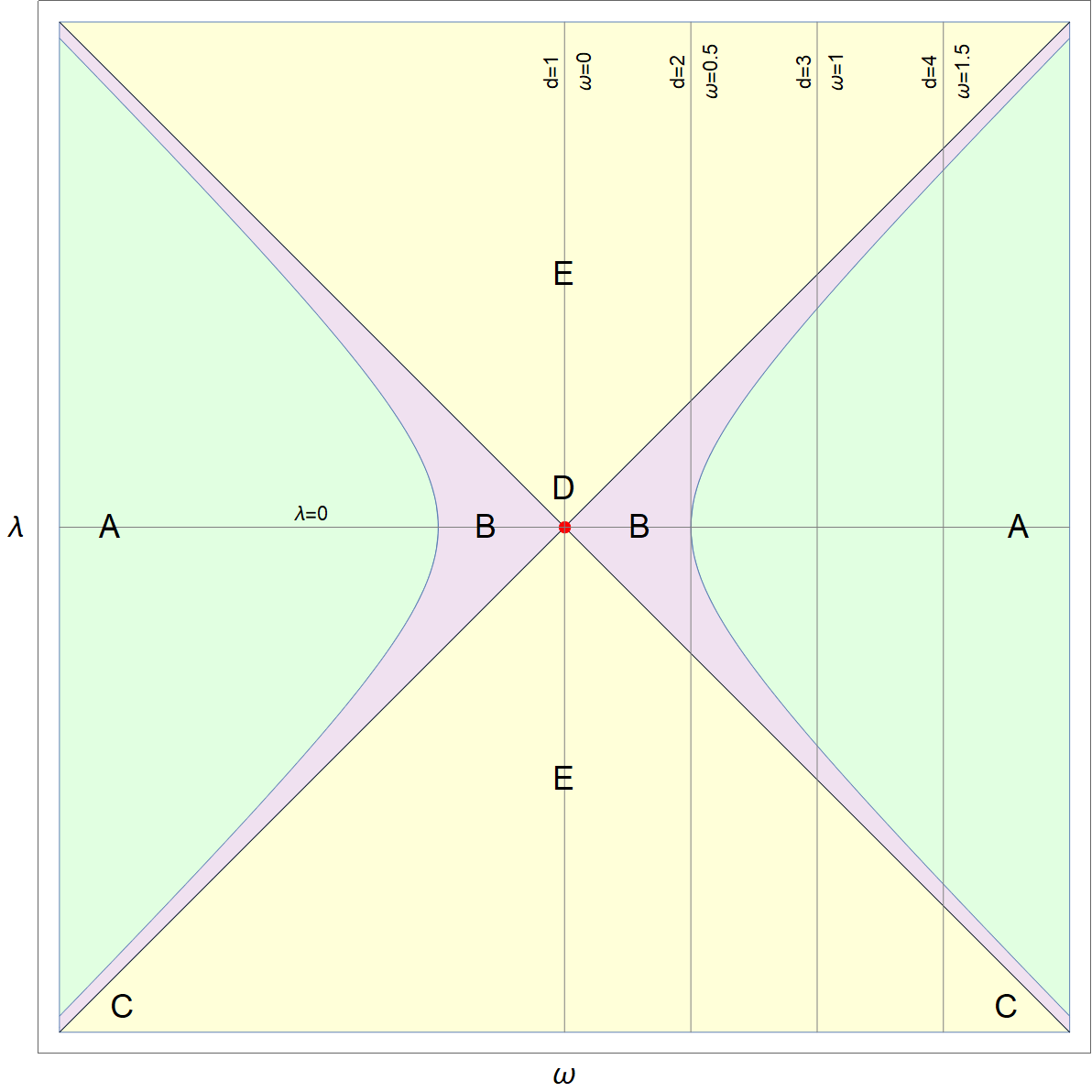
Figure 1: Phase diagram of operators $D_{\omega,\lambda}$ for $(\omega,\lambda)\in\mathbb{R}^{2}$. It is partitioned into five subsets corresponding to five possible behaviours, see Propositions 1 and 2 and Figure 3. We label regions as follows. Color green and letter $A$ refer to $\omega^{2}-\lambda^{2}\geq\frac{1}{4}$ (we do not give a separate name to the boundary of this region, although it is also somewhat special). Color blue and letter $B$ refer to the subset $0<\omega^{2}-\lambda^{2}<\frac{1}{4}$. Black lines and letter $C$ refer to the lines $\omega=\pm\lambda$, except for the special point $(\omega,\lambda)=(0,0)$, which is marked with a fat red dot and letter $D$. Yellow color and letter $E$ are used for the region $\omega^{2}-\lambda^{2}<0$. In addition we present lines corresponding to the lowest angular momentum values for dimensions $d=0$, $d=1$, $d=2$ and $d=3$. Here we disregard the possible sign of $\omega$, which is irrelevant due to symmetry $\omega\mapsto-\omega$.

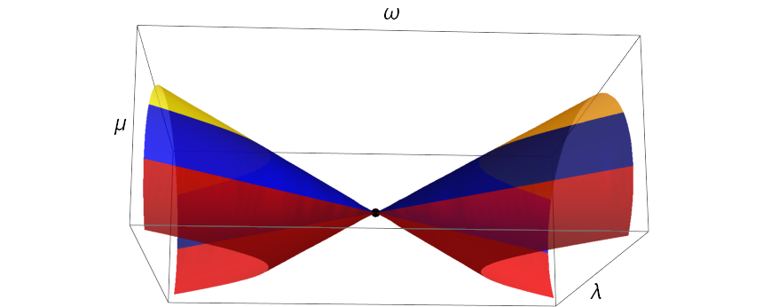
Figure 2: Parameter space of homogeneous self-adjoint Dirac-Coulomb Hamiltonians projected onto axes $\omega,\lambda,\mu$. Regions colored yellow, blue and red are described by inequalities $\mu>\frac{1}{2}$, $0<\mu<\frac{1}{2}$ and $-\frac{1}{2}<\mu<0$, respectively. The fat dot at the origin represents a circle contained in the zero fiber $\mathcal{Z}$, so the whole parameter space is topologically a cylinder.

The operator $D_{\omega,\lambda}^{\min}$ is Hermitian (symmetric with respect to the scalar product $(\cdot|\cdot)$) if and only if $\omega,\lambda\in\mathbb{R}$. Below we state our main results about self-adjoint realizations of $D_{\omega,\lambda}$ in the form of two propositions. They are immediate consequences of the results of Sections 4, 5. We present also the phase diagram of operators $D_{\omega,\lambda}$ on Figure 1 and the parameter space of homogeneous self-adjoint Dirac-Coulomb Hamiltonians on Figure 2.

Let $H^{1}(\mathbb{R}_{+})$ be the first Sobolev space on $\mathbb{R}_{+}$ and $H_{0}^{1}(\mathbb{R}_{+})$ be the closure of $C_{\mathrm{c}}^{\infty}$ in $H^{1}(\mathbb{R}_{+})$.

Proposition 1.

Let $\omega,\lambda\in\mathbb{R}$. The Hermitian operator $D_{\omega,\lambda}^{\min}$ has the following properties.

1. If $\frac{1}{4}\leq\omega^{2}-\lambda^{2}$, it is self-adjoint and $D_{\omega,\lambda}^{\min}=D_{\omega,\lambda,\sqrt{\omega^{2}-\lambda^{2}}}$

2. If $\omega^{2}-\lambda^{2}<\frac{1}{4}$, it has deficiency indices $(1,1)$. Hence there exists a circle of self-adjoint extensions.

Proposition 2.

1. If $\frac{1}{4}<\omega^{2}-\lambda^{2}$, we have $\mathrm{Dom}(D_{\omega,\lambda}^{\min})=H_{0}^{1}(\mathbb{R}_{+},\mathbb{C}^{2})$.

2. If $\frac{1}{4}=\omega^{2}-\lambda^{2}$, we have $H_{0}^{1}(\mathbb{R}_{+},\mathbb{C}^{2})\subsetneq\mathrm{Dom}(D_{\omega,\lambda}^{\min})$.

3. If $0<\omega^{2}-\lambda^{2}<\frac{1}{4}$, exactly two self-adjoint extensions of $D_{\omega,\lambda}^{\min}$ are homogeneous, namely $D_{\omega,\lambda,\sqrt{\omega^{2}-\lambda^{2}}}$ and $D_{\omega,\lambda,-\sqrt{\omega^{2}-\lambda^{2}}}$. The former is distinguished among all self-adjoint extensions by

   $$\int_{0}^{\infty}\left(\frac{|f(x)|^{2}}{x}+|f(x)||f^{\prime}(x)|\right)\mathrm{d}x<\infty\text{ for }f\in\mathrm{Dom}(D_{\omega,\lambda,\sqrt{\omega^{2}-\lambda^{2}}}),$$ (1.7)

   i.e. elements of its domain have finite expectation values of kinetic and potential energy.

4. If $|\lambda|=|\omega|\neq 0$, exactly one self-adjoint extension of $D_{\omega,\lambda}^{\min}$ is homogeneous, namely $D_{\omega,\lambda,0}$. It has the property $H_{0}^{1}(\mathbb{R}_{+},\mathbb{C}^{2})\subsetneq\mathrm{Dom}(D_{\omega,\lambda,0})\subsetneq H^{1}(\mathbb{R}_{+},\mathbb{C}^{2})$.

5. If $\lambda=\omega=0$, all self-adjoint extensions of $D_{\omega,\lambda}^{\min}$ are homogeneous. They have the form $D_{[a:b]}$ with $[a:b]\in\mathbb{RP}^{1}$.

6. If $|\lambda|>|\omega|$, none of self-adjoint extensions of $D_{\omega,\lambda}^{\min}$ is homogeneous.

Now let $\omega,\lambda$ be real and suppose that $\omega^{2}-\lambda^{2}<\frac{1}{4}$. Let $\tau\mapsto U_{\tau}$ denote the scaling transformation. The parameter space of self-adjoint extensions is a circle. It admits an action of the scaling group given by

$$D\mapsto U_{\tau}DU_{\tau}^{-1}.$$ (1.8)

The fixed points of this action are the homogeneous self-adjoint extensions. Main properties of this action are illustrated by Figure 3.

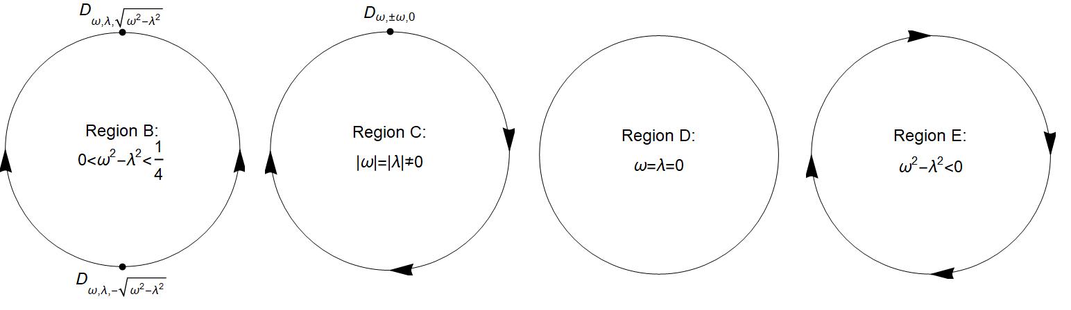
Figure 3: Visualization of the action of the scaling group on self-adjoint extensions of $D_{\omega,\lambda}^{\min}$ in four regions covering the set of $\omega,\lambda$ satisfying $\omega^{2}-\lambda^{2}<\frac{1}{4}$. Fat dots are the fixed points, while arrowheads indicate the direction of the flow as $\tau$ increases, see (1.8). In the first region there are two fixed points, attractive and repulsive, corresponding to a positive and negative $\mu$, respectively. As $\omega^{2}-\lambda^{2}$ decreases to zero, the two fixed points merge to one degenerate fixed point, except for the point $\omega=\lambda=0$ at which the scaling action becomes trivial. As $\omega^{2}-\lambda^{2}$ decreases below zero, the scaling action becomes periodic with period $\frac{\pi}{\sqrt{\lambda^{2}-\omega^{2}}}$.

As we present in Appendix B, $d$-dimensional Dirac-Coulomb Hamiltonians can be reduced to the radial operator (1.1). Combined with the analysis presented above, one obtains rather complete information about self-adjointness and homogeneity properties of these operators. Here we point out only a few facts concerning these extensions on the lowest angular momentum sector.

• dimension $1$: There exist no homogeneous self-adjoint realizations for any $\lambda\neq 0$.

• dimension $2$: The operator defined on smooth spinor-valued functions with compact support not containing zero is not essentially self-adjoint for any $\lambda\neq 0$. For $|\lambda|<1$ there exist homogeneous self-adjoint extensions of $D_{\omega,\lambda}^{\min}$. These homogeneous extensions can be organized into two continuous families. The (more physical) family is defined on $[-1,1]$. At the endpoints $\lambda=\pm 1$ it meets the other family, which is defined on $[-1,0[\cup]0,1]$.

• dimension $d\geq 3$: The operator defined as above is essentially self-adjoint if $\lambda^{2}\leq\frac{d(d-2)}{4}$. If $\frac{d(d-2)}{4}<\lambda^{2}$ it is not essentially self-adjoint. However, for $\lambda^{2}\leq\frac{(d-1)^{2}}{4}$ there exists homogeneous self-adjoint extensions of $D_{\omega,\lambda}^{\min}$. They can be organized into two families depending continuously on $\lambda$. The more physical family is defined on $[-\frac{(d-1)^{2}}{4},\frac{(d-1)^{2}}{4}]$. The second family meets the first at the endpoints and is defined on $[-\frac{(d-1)^{2}}{4},-\frac{d(d-2)}{4}[\,\cup\,]\frac{d(d-2)}{4},\frac{(d-1)^{2}}{4}].$

In all cases in which there exist no homogeneous self-adjoint extensions, the defect indices are nevertheless equal and hence there exist nonhomogeneous self-adjoint extensions.

Analysis of self-adjoint realizations of the 3-dimensional Dirac-Coulomb Hamiltonian has a long and rich history in the mathematical literature. There even exists a recent review paper devoted to this subject [24]. Let us explain the main points of this history, refering the reader to [24] for more details.

A direct application of the Kato-Rellich theorem yields the essential self-adjointness of the (massive, 3d) Dirac-Coulomb Hamiltonian only for $|\lambda|<\frac{1}{2}$. This proof is due to Kato [31, 32]. The essential self-adjointness up to the boundary of the “regular region” $|\lambda|<\frac{\sqrt{3}}{2}$ was proven independently by Gustaffson-Rejtö [29, 37] and Schmincke [39]. They needed to use slightly more refined arguments going beyond to the basic Kato-Rellich theorem. The “distinguished self-adjoint extension” in the region $\frac{\sqrt{3}}{2}<|\lambda|<1$ was described in several equivalent ways, mostly involving the characterization of the domain, by Schmincke, Wüst, Klaus, Nenciu and others [40, 45, 46, 36, 25, 5, 6]. The characterization of distinguished self-adjoint extensions based on holomorphic families of operators was first proposed by Kato in [33]. Esteban and Loss [20] characterized the distinguished self-adjoint realization at the boundary of the “transitory region”, that is for $|\lambda|=1$, by using the so-called Hardy-Dirac inequalities. Self-adjoint realizations in the “supercritical region” $|\lambda|>1$ were first studied by Hogreve in [30], and then (with some corrections) in [25]. The authors of [25] analyze also the second distinguished branch of self-adjoint extensions in the critical region, which they call “mirror distinguished”. [5, 6] include in their analysis a term proportional to $\frac{1}{r^{2}}\beta\alpha_{i}x_{i}$, which they call “anomalous magnetic”.

Our treatment of Dirac-Coulomb Hamiltonians is quite different from the above references. We use exact solvability to describe rather completely their resolvent, domain and (stationary) scattering theory. We do not add the mass term, which helps with exact solvability and makes possible to use the homogeneity as a good criterion for distinguished realizations. Another concept which we use is that of a holomorphic family of operators, which we view as an important criterion for distinguishing a realization. The mass term is bounded, so it does not affect the basic picture of distinguished realizations. Our analysis includes realizations which are not necessarily self-adjoint, but turn out to be self-transposed with respect to a natural complex bilinear form. Our description of various closed realizations of Dirac-Coulomb Hamiltonians is quite straightforward and involves only elementary functions. We use neither the von Neumann nor the Krein-Vishik theory theory of self-adjoint extensions, which lead to a rather complicated description of the domains of closed description involving Whittaker functions, see [25, 26].

Our analysis of Dirac-Coulomb Hamiltonians can be viewed as a continuation of a series of papers about holomorphic families of certain 1-dimensional Hamiltonians: Bessel operators [3, 12] and Whittaker operators [13, 10].

Let us mention some more papers, where Dirac-Coulomb operators play an important role.

First, there exists a number of papers [16, 42, 27, 7] devoted to the time dependent approach to scattering theory for self-adjoint Dirac Hamiltonians on $\mathbb{R}^{3}$ with long range potentials.

There also exists a large and interesting literature devoted to eigenvalues inside a spectral gap of a self-adjoint operator, with massive Dirac-Coulomb Hamiltonians as prime examples [20, 21, 38, 26]. Massless Dirac-Coulomb Hamiltonians do not have a gap, and eigenvalues are possible only in non-self-adjoint nonhomogeneous cases. Nevertheless, we believe that methods of our paper are relevant for the eigenvalue problem in the massive self-adjoint case.

For a study of one-dimensional Dirac operators with locally integrable complex potentials, see [2].

Finally, let us mention another interesting related topic, where the question of distinguished self-adjoint realizations arises: 2-body Dirac-Coulomb Hamiltonians. Their mathematical study was undertaken in [8]. Even though the physical significance of these Hamiltonians is not very clear, they are widely used in quantum chemistry.

Let us briefly describe the organization of our paper. Its main part, that is Sections 2–8 describes realizations of 1d Dirac-Coulomb Hamiltonians on $L^{2}(\mathbb{R}_{+},\mathbb{C}^{2})$ focusing on the homogeneous ones. Besides, our paper contains four appendices, which can be read independently.

Appendix A first discusses some general concepts related to 1d Dirac operators. Then two special classes of 1d Dirac-Coulomb Hamiltonians are analyzed in detail.

Essentially all papers that we mentioned in our bibliographical sketch treat the 3-dimensional case. It was pointed out in [28] that a general $d$-dimensional spherically symmetric Dirac Hamiltonian can be reduced to a 1-dimensional one. We describe this reduction in detail in Appendix B. We also analyze its various group-theoretical and differential-geometric aspects, including the relation to Dirac operators on spheres and the famous Lichnerowicz formula. Spectra of the latter are computed in two independent ways and a construction of eigenvectors is presented.

The short Appendix C is devoted to the Mellin transformation.

Finally, in Appendix D we collect properties of various special functions, mostly, Whittaker functions, which are used in our paper. We mostly follow the conventions of [13, 10].

1.1 Remarks about notation

Symbol $(\cdot|\cdot)$ is used for standard scalar products on $L^{2}$ spaces, linear in the second argument, while $\langle\cdot|\cdot\rangle$ is used for the analogous bilinear forms in which complex conjugation is omitted:

$$\langle f|g\rangle=\int f(x)^{\mathrm{T}}g(x)\mathrm{d}x.$$ (1.9)

Tranpose (denoted by the superscript $\scriptstyle\mathrm{T}$) of a densely defined operator is defined in terms of $\langle\cdot|\cdot\rangle$ in the same way as the adjoint (denoted by $*$) is defined in terms of the scalar product. We use superscript $\mathrm{perp}$ for orthogonal complement with respect to $\langle\cdot|\cdot\rangle$ and $\perp$ for orthogonal complement with respect to $(\cdot|\cdot)$. Overline always denotes complex conjugation, for example we have $X^{\perp}=\overline{X^{\mathrm{perp}}}$ for a subspace $X$.

We will write $\mathbb{R}_{+}=]0,\infty[$, $\mathbb{C}_{\pm}=\{z\in\mathbb{C}\,|\,\pm\mathrm{Im}(z)>0\}$, $\mathbb{N}=\{0,1,\dots\}$. Omission of zero will be denoted by $\times$, e.g. $\mathbb{R}^{\times}=\mathbb{R}\backslash\{0\}$. Indicator function of a subset $S\subset\mathbb{R}$ will be denoted by ${\mathchoice{\rm 1\mskip-4.0mul}{\rm 1\mskip-4.0mul}{\rm 1\mskip-4.5mul}{\rm 1\mskip-5.0mul}}_{S}$. We label elements of the Riemann sphere $\mathbb{CP}^{1}$ using homogeneous coordinates, i.e. $[a:b]\in\mathbb{CP}^{1}$ is the complex line spanned by $(a,b)\in\mathbb{C}^{2}\backslash\{0\}$.

Operators of multiplication of a function in $L^{2}(\mathbb{R}_{+},\mathbb{C}^{n})$ and $L^{2}(\mathbb{R},\mathbb{C}^{n})$ by its argument will be denoted by $X$ and $K$, respectively. Dilation group action on $L^{2}(\mathbb{R}_{+},\mathbb{C}^{n})$ is defined by $U_{\tau}f(x)=\mathrm{e}^{\frac{\tau}{2}}f(\mathrm{e}^{\tau}x)$. We denote its self-adjoint generator by $A$, so that $U_{\tau}=\mathrm{e}^{\mathrm{i}\tau A}$. Operator $O$ is said to be homogeneous of degree $\nu$ if $U_{\tau}OU_{\tau}^{-1}=\mathrm{e}^{\nu\tau}O$. Inversion operator $J$ is defined by $(Jf)(x)=\frac{1}{x}f\left(\frac{1}{x}\right)$. It is unitary and satisfies $J^{2}=1$, $JAJ^{-1}=-A$.

Complex power functions $z\mapsto z^{a}$ are holomorphic and defined on $\mathbb{C}\backslash]-\infty,0]$. Domains of holomorphy of special functions used in the text are specified in Appendix D.

In our paper we will often use the concept of a holomorphic map with values in closed operators, which we now briefly recall [32, 14]. We will give two equivalent definitions of this concept: the first is “more elegant”, the second “more practical”. To formulate the first definition note that the Grassmannian (the set of closed subspaces) $\mathrm{Grass}(X)$ of a Hilbert space $X$ carries the structure of a complex Banach manifold [17].

Consider Hilbert spaces $X_{2},X_{3}$ be Hilbert spaces and a complex manifold $\mathcal{M}$. We say that a function $\mathcal{M}\ni p\mapsto T_{p}$ of closed operators $X_{2}\to X_{3}$ is holomorphic if and only if $p\mapsto\mathrm{graph}(T_{p})\in\mathrm{Grass}(X_{2}\times X_{3})$ is a holomorphic map.

Equivalently, $\mathcal{M}\ni p\mapsto T_{p}$ is holomorphic if for every $p_{0}\in\mathcal{M}$ there exists a neighborhood $\mathcal{M}_{0}$ of $p_{0}$ in $\mathcal{M}$, a Hilbert space $X_{1}$ and a holomorphic family $\mathcal{M}_{0}\ni p\mapsto S_{p}$ of bounded injective operators $S_{p}:X_{1}\to X_{2}$ such that $\mathrm{Ran}(S_{p})=\mathrm{Dom}(T_{p})$ and $T_{p}S_{p}$ form a holomorphic family of bounded operators.

2 Blown-up quadric

Formal Dirac-Coulomb Hamiltonians depend on parameters $(\omega,\lambda)\in\mathbb{C}^{2}$. In order to specify their realizations as closed homogeneous operators, it is necessary to choose a square root of $\omega^{2}-\lambda^{2}$. For this reason homogeneous Dirac-Coulomb Hamiltonians are parametrized by points of a certain complex manifold. This section is devoted to its definition and basic properties.

Let us first introduce a certain null quadric in $\mathbb{C}^{3}$:

$$\mathcal{M}^{\mathrm{pre}}:=\left\{(\omega,\lambda,\mu)\in\mathbb{C}^{3}\,|\,\omega^{2}=\lambda^{2}+\mu^{2}\right\}.$$ (2.1)

By the holomorphic implicit function theorem, $\mathcal{M}^{\mathrm{pre}}$ is a complex two-dimensional submanifold of $\mathbb{C}^{3}$ away from the singular point $(0,0,0)$ (also denoted $0$ for brevity).

We consider also the so-called blowup of $\mathcal{M}^{\mathrm{pre}}$ at the singular point, defined by

$$\mathcal{M}=\left\{(\omega,\lambda,\mu,[a:b])\in\mathbb{C}^{3}\times\mathbb{CP}^{1}\,|\,\begin{bmatrix}\omega+\lambda&\mu\\ \mu&\omega-\lambda\end{bmatrix}\begin{bmatrix}a\\ b\end{bmatrix}=\begin{bmatrix}0\\ 0\end{bmatrix}\right\}.$$ (2.2)

Fibers of the projection map $\mathcal{M}\to\mathbb{CP}^{1}$ are described by triples $(\omega,\lambda,\mu)\in\mathbb{C}^{3}$ subject to two linearly independent linear equations, whose coefficients are holomorphic functions on local coordinate patches of $\mathbb{CP}^{1}$. Therefore $\mathcal{M}$ is a holomorphic line bundle over $\mathbb{CP}^{1}$, embedded in the trivial bundle $\mathbb{C}^{3}\times\mathbb{CP}^{1}$. In particular it is a two-dimensional complex manifold.

Equation $\begin{bmatrix}\omega+\lambda&\mu\\ \mu&\omega-\lambda\end{bmatrix}\begin{bmatrix}a\\ b\end{bmatrix}=\begin{bmatrix}0\\ 0\end{bmatrix}$ has a solution different than $(a,b)=(0,0)$ if and only if the quadratic equation defining $\mathcal{M}^{\mathrm{pre}}$ is satisfied. Thus there is a projection map $\mathcal{M}\to\mathcal{M}^{\mathrm{pre}}$. Its restriction to the preimage of $\mathcal{M}^{\mathrm{pre}}\backslash\{0\}$ is an isomorphism and will be treated as an identification. The preimage of zero, called the zero fiber and denoted $\mathcal{Z}$, is an isomorphic copy of $\mathbb{CP}^{1}$.

We will often use the short notation $p=(\omega,\lambda,\mu,[a:b])$ for elements of $\mathcal{M}$. If $p\notin\mathcal{Z}$, then $[a:b]$ is uniquely determined by $(\omega,\lambda,\mu)$ and we abbreviate $p=(\omega,\lambda,\mu)$. In turn for $p$ in the zero fiber we write $p=[a:b]$.

We will now describe useful coordinate systems on $\mathcal{M}$. The coordinates

$$z=\frac{a}{b},\qquad\omega+\lambda$$ (2.3)

are valid on $\{b\neq 0\}$ – the open subset of $\mathcal{M}$ which is the complement of

$$\{b=0\}=\{(\omega,-\omega,0,[1:0])\}_{\omega\in\mathbb{C}}.$$ (2.4)

More precisely, the following map is an isomorphism of complex manifolds:

$$\mathbb{C}^{2}\ni(\omega+\lambda,z)\mapsto\left(\frac{(\omega+\lambda)(1+z^{2})}{2},\frac{(\omega+\lambda)(1-z^{2})}{2},-(\omega+\lambda)z,[z:1]\right)\in\{b\neq 0\}.$$ (2.5)

We note that

$$z=-\frac{\mu}{\omega+\lambda}=-\frac{\omega-\lambda}{\mu}$$ (2.6)

whenever the denominators are nonzero.

Analogously, on $\{a\neq 0\}$, the complement of

$$\{a=0\}=\{(\omega,\omega,0,[0:1])\}_{\omega\in\mathbb{C}},$$ (2.7)

we use the coordinates $z^{-1}$ and $\omega-\lambda$.

Sets $\{a\neq 0\}$, $\{b\neq 0\}$ cover the whole $\mathcal{M}$. On their intersection we have

$$\omega-\lambda=(\omega+\lambda)z^{2}.$$ (2.8)

We note that the locus $\{\lambda=0\}$ is the union of three Riemann surfaces:

$$\{\lambda=0\}=\mathcal{Z}\cup\{a=b\}\cup\{a=-b\}.$$ (2.9)

It is singular at the intersection points:

$$\{[1:1]\}=\mathcal{Z}\cap\{a=b\},\quad\{[1:-1]\}=\mathcal{Z}\cap\{a=-b\}.$$ (2.10)

On the other hand, the level sets $\{\lambda=\lambda_{0}\}$ with $\lambda_{0}\neq 0$ are nonsingular. Similarly, we have

$$\{\mu=0\}=\mathcal{Z}\cup\{a=0\}\cup\{b=0\}.$$ (2.11)

Remark 3.

Consider the tautological line bundle $\mathcal{N}\to\mathbb{CP}^{1}$, i.e. the space of pairs ${\big{(}(a^{\prime},b^{\prime}),[a:b]\big{)}\in\mathbb{C}^{2}\times\mathbb{CP}^{1}}$ such that $(a^{\prime},b^{\prime})\in[a:b]$. Setting $z:=\frac{a^{\prime}}{b^{\prime}}$, we obtain two charts $(b^{\prime},z)$ and $(a^{\prime},z^{-1})$, which cover $\mathcal{N}$. The clutching formula for $\mathcal{N}$ is $a^{\prime}=b^{\prime}z$, which can be compared with the clutching formula (2.8) for $\mathcal{M}$. Thus we see that as a holomorphic vector bundle $\mathcal{M}$ is isomorphic to the tensor square of $\mathcal{N}$.

Later we will encounter the meromorphic functions on $\mathcal{M}$

$$N_{p}^{\pm}=\frac{z\pm\mathrm{i}}{\Gamma(1+\mu\mp\mathrm{i}\lambda)}.$$ (2.12)

We define the exceptional sets as their zero loci:

$$\mathcal{E}^{\pm}:= \{N_{p}^{\pm}=0\}=\bigcup_{n=0}^{\infty}\mathcal{E}_{n}^{\pm},$$ (2.13)

$$\mathcal{E}_{0}^{\pm}:= \{p\in\mathcal{M}\,|\,a=\mp\mathrm{i}b\}=\{p\in\mathcal{M}\,|\,z=\mp\mathrm{i}\},$$

$$\mathcal{E}_{n}^{\pm}:= \{p\in\mathcal{M}\,|\,\mu\mp\mathrm{i}\lambda=-n\},\quad n=1,2,\dots.$$

Away from $\mathcal{Z}$, the condition $p\in\mathcal{E}_{0}^{\pm}$ is equivalent to $\mu\mp\mathrm{i}\lambda=0$. Thus for $p\notin\mathcal{Z}$ we have $p\in\mathcal{E}^{\pm}$ if and only if $\mu\mp\mathrm{i}\lambda\in-\mathbb{N}$. Moreover,

$$\mathcal{E}^{\pm}\cap\mathcal{Z}=\mathcal{E}_{0}^{\pm}\cap\mathcal{Z}=\{[\mp\mathrm{i}:1]\}.$$ (2.14)

In particular $\mathcal{Z}\cap\mathcal{E}^{+}\cap\mathcal{E}^{-}=\emptyset$. Clearly, the sets $\mathcal{E}_{n}^{\pm}$, $n=0,1,2,\dots$, are connected components of $\mathcal{E}^{\pm}$. Each $\mathcal{E}_{n}^{\pm}$ is isomorphic to $\mathbb{C}$. Indeed, $\mathcal{E}_{0}^{\pm}$ is a fiber of $\mathcal{M}\to\mathbb{CP}^{1}$ and $\mathcal{E}_{n}^{\pm}$ with $n\geq 1$ is globally parametrized by $\omega$.

Lemma 4.

$\mathcal{E}^{+}\cap\mathcal{E}^{-}$ is a countably infinite discrete subset of $\mathcal{M}$ on which $2\mu+1\in-\mathbb{N}$. In particular $\mu\leq-\frac{1}{2}$.

Proof.

Suppose that $p\in\mathcal{M}$ is such that $\mu+\mathrm{i}\lambda=-n$, $\mu-\mathrm{i}\lambda=-m$ with $n,m\in\mathbb{N}$. Then

$$(\omega,\lambda,\mu)=\left(\pm nm,\frac{m-n}{2\mathrm{i}},-\frac{m+n}{2}\right),\qquad(n,m)\in\mathbb{N}^{2}\backslash\{(0,0)\},$$ (2.15)

from which the discreteness and countability of $\mathcal{E}^{+}\cap\mathcal{E}^{-}$ is clear. If both $n,m$ are zero, then $\mu=\lambda=0$ and hence also $\omega=0$. In this case we have $p\in\mathcal{Z}\cap\mathcal{E}^{+}\cap\mathcal{E}^{-}=\emptyset$—contradiction. Thus at least one of $n,m$ is nonzero, and we have $2\mu+1=1-n-m\in-\mathbb{N}$. Conversely, if $(n,m)\in\mathbb{N}^{2}$ is different than $(0,0)$, then (2.15) defines one or two (if $nm\neq 0$) points of $\mathcal{E}^{+}\cap\mathcal{E}^{-}$, so this set is infinite. ∎

We define the principal scattering amplitude as the ratio

$$S_{p}=\frac{N_{p}^{-}}{N_{p}^{+}}=\frac{z-\mathrm{i}}{z+\mathrm{i}}\frac{\Gamma(1+\mu-\mathrm{i}\lambda)}{\Gamma(1+\mu+\mathrm{i}\lambda)}=\frac{(\omega-\lambda+\mathrm{i}\mu)\Gamma(1+\mu-\mathrm{i}\lambda)}{(\omega-\lambda-\mathrm{i}\mu)\Gamma(1+\mu+\mathrm{i}\lambda)}.$$ (2.16)

It satisfies $\overline{S_{\overline{p}}}=S_{p}^{-1}$, hence it has a unit modulus for $p=\overline{p}$. Furthermore,

$$\mathcal{E}^{-}\backslash\mathcal{E}^{+}=\{S_{p}=0\},\qquad\mathcal{E}^{+}\backslash\mathcal{E}^{-}=\{S_{p}=\infty\},\qquad\mathcal{E}^{-}\cap\mathcal{E}^{+}=\{S_{p}\text{ indeterminate}\}.$$ (2.17)

We introduce an involution on $\mathcal{M}$ by

$$\tau(\omega,\lambda,\mu,[a:b])=(\omega,\lambda,-\mu,[-a:b]).$$ (2.18)

3 Eigenfunctions and Green’s kernels

3.1 Zero energy

The 1d Dirac-Coulomb Hamiltonian with parameters $\omega,\lambda\in\mathbb{C}$ is given by the expression

$$D_{\omega,\lambda}=\begin{bmatrix}-\frac{\lambda+\omega}{x}&-\partial_{x}\\ \partial_{x}&-\frac{\lambda-\omega}{x}\end{bmatrix}.$$ (3.1)

When we consider (3.1) as acting on distributions on $\mathbb{R}_{+}$, we will call it the formal operator. In what follows we will define various realizations of this operator, with domain and range contained in $L^{2}(\mathbb{R}_{+},\mathbb{C}^{2})$, preferably closed. They will have additional indices.

First consider its eigenequation for eigenvalue zero

$$D_{\omega,\lambda}\xi=0.$$ (3.2)

The space of distributions on $\mathbb{R}_{+}$ solving (3.2) will be denoted $\mathrm{Ker}(D_{\omega,\lambda})$. The following lemma shows that $\mathrm{Ker}(D_{\omega,\lambda})$ consists of smooth solutions.

Lemma 5.

Let $f$ be a distributional solution on $\mathbb{R}_{+}$ of the equation $f^{\prime}(x)=M(x)f(x)$ for some $M\in C^{\infty}(\mathbb{R}_{+},\mathrm{End}(\mathbb{C}^{n}))$. Then $f$ is a smooth function.

Proof.

Fix $x_{0}\in\mathbb{R}_{+}$ and $\epsilon\in\left]0,\frac{x_{0}}{2}\right[$. We choose $\chi_{2}\in C_{c}^{\infty}(\mathbb{R}_{+})$ equal to $1$ on $[x_{0}-2\epsilon,x_{0}+2\epsilon]$ and $\chi_{1}\in C_{c}^{\infty}(\mathbb{R}_{+})$ supported in $[x_{0}-2\epsilon,x_{0}+2\epsilon]$ and equal to $1$ on $[x_{0}-\epsilon,x_{0}+\epsilon]$. Clearly $\chi_{2}\chi_{1}=\chi_{1}$ and $\chi_{2}\chi_{1}^{\prime}=\chi_{1}^{\prime}$. Put $f_{j}=\chi_{j}f$ for $j=1,2$. Since $f_{2}$ is compactly supported, it belongs to $H^{s}(\mathbb{R}_{+},\mathbb{C}^{n})$ for some $s\in\mathbb{R}$. We have $f_{1}=\chi_{1}f_{2}$, so also $f_{1}\in H^{s}(\mathbb{R}_{+},\mathbb{C}^{n})$. Now evaluate

$$f_{1}^{\prime}=\chi_{1}^{\prime}f+\chi_{1}f^{\prime}=\chi_{2}\chi_{1}^{\prime}f+\chi_{2}\chi_{1}Mf=(\chi_{1}^{\prime}+\chi_{1}M)f_{2}.$$ (3.3)

Since $\chi_{1}^{\prime}+\chi_{1}M\in C_{c}^{\infty}(\mathbb{R}_{+})$, this implies that $f_{1}\in H^{s+1}(\mathbb{R}_{+},\mathbb{C}^{n})$. Next we may repeat this argument with $\frac{\epsilon}{2}$ playing the role of new $\epsilon$, $\chi_{1}$ as the new $\chi_{2}$ and arbitrarily chosen new $\chi_{1}$. Then the new $f_{1}$ is in $H^{s+2}(\mathbb{R}_{+},\mathbb{C}^{n})$. Proceeding like this inductively we conclude that for every $s\in\mathbb{R}$ there exists $\chi\in C_{c}^{\infty}(\mathbb{R}_{+})$ equal to $1$ on a neighbourhood of $x_{0}$ such that $\chi\,f$ belongs to $H^{s}(\mathbb{R}_{+},\mathbb{C}^{n})$. Taking $s>\frac{1}{2}+k$ we conclude from Sobolev embeddings that $f$ is of class $C^{k}$ on a neighbourhood of $x_{0}$, perhaps after modifying it on a set of measure zero. Since this is true for every $k\in\mathbb{N}$ and every $x_{0}\in\mathbb{R}_{+}$, $f$ is smooth. ∎

For $p\in\mathcal{M}$, we introduce two types of solutions of (3.2):

$$\eta_{p}^{\uparrow}(x) :=\frac{x^{\mu}}{\omega+\lambda}\begin{bmatrix}-\mu\\ \omega+\lambda\end{bmatrix}=x^{\mu}\begin{bmatrix}z\\ 1\end{bmatrix},$$ (3.4a)

$$\eta_{p}^{\downarrow}(x) :=\frac{x^{\mu}}{\omega-\lambda}\begin{bmatrix}\omega-\lambda\\ -\mu\end{bmatrix}=x^{\mu}\begin{bmatrix}1\\ z^{-1}\end{bmatrix}.$$ (3.4b)

They are nowhere vanishing meromorphic functions of $p$ for every $x$:

$$\mathcal{M}\ni p\mapsto\eta_{p}^{\uparrow}(x) \quad\text{has a pole on }\{b=0\},$$

$${\mathcal{M}}\ni p\mapsto\eta_{p}^{\downarrow}(x) \quad\text{has a pole on }\{a=0\}.$$

On $\{a\neq 0\}\cap\{b\neq 0\}$ we have $\eta_{p}^{\downarrow}=z^{-1}\eta_{p}^{\uparrow}$.

There exist also exceptional solutions, defined only for $\mu=0$:

$$\vartheta_{\omega}^{\uparrow}(x) :=-\ln(x)\begin{bmatrix}0\\ 2\omega\end{bmatrix}+\begin{bmatrix}1\\ 0\end{bmatrix},\quad\omega-\lambda=0;$$ (3.5a)

$$\vartheta_{\omega}^{\downarrow}(x) :=-\ln(x)\begin{bmatrix}2\omega\\ 0\end{bmatrix}+\begin{bmatrix}0\\ 1\end{bmatrix},\quad\omega+\lambda=0.$$ (3.5b)

The nullspace of $D_{\omega,\lambda}$, that is, $\mathrm{Ker}(D_{\omega,\lambda})$ has the following bases:

$$\mu\neq 0: \qquad\big{(}\eta_{\omega,\lambda,\mu}^{\uparrow},\quad\eta_{\omega,\lambda,-\mu}^{\uparrow}\big{)}\quad\text{and}\quad\big{(}\eta_{\omega,\lambda,\mu}^{\downarrow},\quad\eta_{\omega,\lambda,-\mu}^{\downarrow}\big{)},$$

$$\omega=\lambda\neq 0: \qquad\big{(}\eta_{\omega,\omega,0}^{\uparrow},\quad\vartheta_{\omega}^{\uparrow}\big{)},$$

$$\omega=-\lambda\neq 0: \qquad\big{(}\eta_{\omega,-\omega,0}^{\downarrow},\quad\vartheta_{\omega}^{\downarrow}\big{)},$$

$$(\omega,\lambda)=(0,0): \qquad\big{(}\vartheta_{0}^{\uparrow},\quad\vartheta_{0}^{\downarrow}\big{)}=\left(\begin{bmatrix}1\\ 0\end{bmatrix},\quad\begin{bmatrix}0\\ 1\end{bmatrix}\right).$$

The canonical bisolution of $D_{\omega,\lambda}$ (A.5) at $k=0$ takes the form

$$G_{\omega,\lambda}^{\leftrightarrow}(0;x,y) =\frac{1}{2}\begin{bmatrix}\frac{\omega-\lambda}{\mu}\Big{(}\Big{(}\frac{x}{y}\Big{)}^{\mu}-\Big{(}\frac{y}{x}\Big{)}^{\mu}\Big{)}&\Big{(}\frac{x}{y}\Big{)}^{\mu}+\Big{(}\frac{y}{x}\Big{)}^{\mu}\\[8.61108pt] -\Big{(}\frac{x}{y}\Big{)}^{\mu}-\Big{(}\frac{y}{x}\Big{)}^{\mu}&-\frac{\omega+\lambda}{\mu}\Big{(}\Big{(}\frac{x}{y}\Big{)}^{\mu}-\Big{(}\frac{y}{x}\Big{)}^{\mu}\Big{)}\end{bmatrix}.$$ (3.6)

3.2 Nonzero energy

Now consider the eigenequation for the eigenvalue $k\in\mathbb{C}^{\times}$:

$$(D_{\omega,\lambda}-k)f=0.$$ (3.7)

Acting on (3.7) with $D_{\omega,-\lambda}+k$ we obtain

$$\begin{bmatrix}-\partial_{x}^{2}+\frac{\omega^{2}-\lambda^{2}}{x^{2}}-\frac{2\lambda k}{x}-k^{2}&\frac{\omega-\lambda}{x^{2}}\\[8.61108pt] \frac{\omega+\lambda}{x^{2}}&-\partial_{x}^{2}+\frac{\omega^{2}-\lambda^{2}}{x^{2}}-\frac{2\lambda k}{x}-k^{2}\end{bmatrix}f(x)=0.$$ (3.8)

At first we focus on the case $\mu^{2}=\omega^{2}-\lambda^{2}\neq 0$, in which $\begin{bmatrix}0&\omega-\lambda\\ \omega+\lambda&0\end{bmatrix}$ is a diagonalizable matrix. Decomposing $f(x)$ in its eigenbasis

$$f(x)=f_{+}(x)\begin{bmatrix}\omega-\lambda\\ \mu\end{bmatrix}+f_{-}(x)\begin{bmatrix}\omega-\lambda\\ -\mu\end{bmatrix}$$ (3.9)

we find that functions $f_{\pm}(x)$ satisfy the Whittaker equations

$$\left(-\partial_{x}^{2}+\frac{\left(\mu\pm\frac{1}{2}\right)^{2}-\frac{1}{4}}{x^{2}}-\frac{2\lambda k}{x}-k^{2}\right)f_{\pm}(x)=0.\\ \$$ (3.10)

This second order differential equation is satisfied by the Whittaker functions (D.15) and (D.18):

$$f_{\pm}(x)=c_{\pm,1}\mathcal{I}_{-\mathrm{i}\lambda,\mu\pm\frac{1}{2}}(2\mathrm{i}kx)+c_{\pm,2}\mathcal{K}_{-\mathrm{i}\lambda,\mu\pm\frac{1}{2}}(2\mathrm{i}kx).$$ (3.11)

For generic values of parameters, the four functions appearing in (3.11) are linearly independent and thus (3.11) is the general solution of (3.8). Inspection of its expansion for $x\to 0$ reveals that (again, for generic parameters) it is annihilated by $D_{\omega,\lambda}-k$ if and only if

$$\mathrm{i}\omega\,c_{-,1}=c_{+,1},\qquad\omega\,c_{-,2}=(\lambda+\mathrm{i}\mu)c_{+,2}.$$ (3.12)

Remark 6.

Equation (3.7) simplifies for $\mu=0$, but instead of treating it separately we will construct solutions valid on the whole $\mathcal{M}$ by analytic continuation. For similar reasons we disregard non-generic cases mentioned above Equation (3.12).

Let us introduce a family of solutions of the eigenequation (3.7) defined for $k\in\mathbb{C}\backslash[0,\mathrm{i}\infty[$:

$$\xi_{p}^{-}(k,x)=\frac{\Gamma(1+\mu+\mathrm{i}\lambda)}{2\mu(\omega-\lambda+\mathrm{i}\mu)}\left(\mathrm{i}\omega\mathcal{I}_{-\mathrm{i}\lambda,\mu+\frac{1}{2}}(2\mathrm{i}kx)\begin{bmatrix}\omega-\lambda\\ \mu\end{bmatrix}+\mathcal{I}_{-\mathrm{i}\lambda,\mu-\frac{1}{2}}(2\mathrm{i}kx)\begin{bmatrix}\omega-\lambda\\ -\mu\end{bmatrix}\right),$$ (3.13a)

$$\zeta_{p}^{-}(k,x)=\frac{\omega\,\mathcal{K}_{-\mathrm{i}\lambda,\mu+\frac{1}{2}}(2\mathrm{i}kx)}{\mu(\omega-\lambda-\mathrm{i}\mu)}\begin{bmatrix}\omega-\lambda\\ \mu\end{bmatrix}+\frac{(\lambda+\mathrm{i}\mu)\mathcal{K}_{-\mathrm{i}\lambda,\mu-\frac{1}{2}}(2\mathrm{i}kx)}{\mu(\omega-\lambda-\mathrm{i}\mu)}\begin{bmatrix}\omega-\lambda\\ -\mu\end{bmatrix}.$$ (3.13b)

As an alternative to the presented derivation, one may check directly that they satisfy (3.7) using recursion relations from Appendix D.4.

The second family, defined for $k\in\mathbb{C}\backslash[0,-\mathrm{i}\infty[$, is obtained by reflection:

$$\xi_{p}^{+}(k,x)=\overline{\xi_{\overline{p}}^{-}(\overline{k},x)},\qquad\zeta_{p}^{+}(k,x)=\overline{\zeta_{\overline{p}}^{-}(\overline{k},x)}.$$ (3.14)

Explicit expressions in terms of Whittaker functions take the form

$$\xi_{p}^{+}(k,x)=\frac{\Gamma(1+\mu-\mathrm{i}\lambda)}{2\mu(\omega-\lambda-\mathrm{i}\mu)}\left(-\mathrm{i}\omega\mathcal{I}_{\mathrm{i}\lambda,\mu+\frac{1}{2}}(-2\mathrm{i}kx)\begin{bmatrix}\omega-\lambda\\ \mu\end{bmatrix}+\mathcal{I}_{\mathrm{i}\lambda,\mu-\frac{1}{2}}(-2\mathrm{i}kx)\begin{bmatrix}\omega-\lambda\\ -\mu\end{bmatrix}\right),$$ (3.15a)

$$\zeta_{p}^{+}(k,x)=\frac{\omega\,\mathcal{K}_{\mathrm{i}\lambda,\mu+\frac{1}{2}}(-2\mathrm{i}kx)}{\mu(\omega-\lambda+\mathrm{i}\mu)}\begin{bmatrix}\omega-\lambda\\ \mu\end{bmatrix}+\frac{(\lambda-\mathrm{i}\mu)\mathcal{K}_{\mathrm{i}\lambda,\mu-\frac{1}{2}}(-2\mathrm{i}kx)}{\mu(\omega-\lambda+\mathrm{i}\mu)}\begin{bmatrix}\omega-\lambda\\ -\mu\end{bmatrix}.$$ (3.15b)

Lemma 7.

Let us fix $k,x$. $\xi^{+}_{p}(k,x)$ and $\xi^{-}_{p}(k,x)$ are meromorphic functions of $p\in\mathcal{M}$, nonsingular away from $\mathcal{E}^{+}$ and $\mathcal{E}^{-}$, respectively. $\zeta_{p}^{+}(k,x)$ and $\zeta_{p}^{-}(k,x)$ are holomorphic functions on the whole $\mathcal{M}$. Furthermore, $\zeta_{p}^{\pm}(\cdot)$ satisfy $\zeta_{p}^{\pm}=\zeta_{\tau(p)}^{\pm}$, where $\tau$ was defined in (2.18), and are nonzero functions for every $p\in\mathcal{M}$.

Proof.

It is sufficient to prove the claim for the family with superscript minus. Meromorphic dependence on $p$ is clear. Definitions of $\xi_{p}^{-}$ and $\zeta_{p}^{-}$ can be manipulated to the form

$$\xi_{p}^{-}(k,x)=\mathrm{i}\,\mathcal{I}_{-\mathrm{i}\lambda,\mu+\frac{1}{2}}(2\mathrm{i}kx)\frac{1}{N_{p}^{-}}\begin{bmatrix}-1\\ z\end{bmatrix}+\frac{\mathcal{I}_{-\mathrm{i}\lambda,\mu-\frac{1}{2}}(2\mathrm{i}kx)-\mathrm{i}\lambda\,\mathcal{I}_{-\mathrm{i}\lambda,\mu+\frac{1}{2}}(2\mathrm{i}kx)}{\mu}\frac{1}{N_{p}^{-}}\begin{bmatrix}z\\ 1\end{bmatrix},$$ (3.16a)

$$\zeta_{p}^{-}(k,x)=\mathcal{K}_{-\mathrm{i}\lambda,\mu+\frac{1}{2}}(2\mathrm{i}kx)\begin{bmatrix}\mathrm{i}\\ 1\end{bmatrix}-\frac{(\omega+\lambda)(z+\mathrm{i})}{2}\frac{\mathcal{K}_{-\mathrm{i}\lambda,\mu-\frac{1}{2}}(2\mathrm{i}kx)-\mathcal{K}_{-\mathrm{i}\lambda,\mu+\frac{1}{2}}(2\mathrm{i}kx)}{\mu}\begin{bmatrix}z\\ 1\end{bmatrix}$$ (3.16b)

$$=\mathcal{K}_{-\mathrm{i}\lambda,\mu-\frac{1}{2}}(2\mathrm{i}kx)\begin{bmatrix}\mathrm{i}\\ 1\end{bmatrix}-\frac{(\omega+\lambda)(-z+\mathrm{i})\big{(}\mathcal{K}_{-\mathrm{i}\lambda,\mu-\frac{1}{2}}(2\mathrm{i}kx)-\mathcal{K}_{-\mathrm{i}\lambda,\mu+\frac{1}{2}}(2\mathrm{i}kx)\big{)}}{2\mu}\begin{bmatrix}-z\\ 1\end{bmatrix}.$$ (3.16c)

Functions $\mu\mapsto\frac{\mathcal{I}_{-\mathrm{i}\lambda,\mu-\frac{1}{2}}(2\mathrm{i}kx)-\mathrm{i}\lambda\,\mathcal{I}_{-\mathrm{i}\lambda,\mu+\frac{1}{2}}(2\mathrm{i}kx)}{\mu}$ and $\mu\mapsto\frac{\mathcal{K}_{-\mathrm{i}\lambda,\mu-\frac{1}{2}}(2\mathrm{i}kx)-\mathcal{K}_{-\mathrm{i}\lambda,\mu+\frac{1}{2}}(2\mathrm{i}kx)}{\mu}$ have removable singularities at $\mu=0$, as seen from identities (D.17), (D.19a). Therefore $\zeta_{p}^{-}(k,x)$ is regular for $z\neq\infty$. If in addition $p\notin\mathcal{E}^{-}$, then also $(N_{p}^{-})^{-1}$ and hence $\xi_{p}^{-}$ is nonsingular.

Next write $(\omega+\lambda)(z+\mathrm{i})\begin{bmatrix}z\\ 1\end{bmatrix}=(\omega-\lambda)(1+\mathrm{i}z^{-1})\begin{bmatrix}1\\ z^{-1}\end{bmatrix}$ in (3.16b). Then it is clear that $\zeta_{p}^{-}(k,x)$ is nonsingular for $z=\infty$.

Moreover, $\frac{z}{N_{p}^{-}}=\Gamma(1+\mu+\mathrm{i}\lambda)(1-\mathrm{i}z^{-1})^{-1}$ is nonsingular for $z=\infty$ if $p\not\in\mathcal{E}_{0}^{-}$. Hence $\xi_{p}^{-}(k,x)$ is nonsingular for $z=\infty$ if $p\notin\mathcal{E}^{-}$.

The statement about the symmetry $\mu\to-\mu$ follows from the comparison of (3.16b) and (3.16c). The last claim follows from (3.19) below. ∎

Remark 8.

Proof of Lemma 7 shows that functions $\frac{\xi_{p}^{\pm}(k,x)}{\Gamma(1+\mu\mp\mathrm{i}\lambda)}$ are singular on subsets of $\mathcal{M}$ smaller than $\mathcal{E}^{\pm}$, namely on $\mathcal{E}_{0}^{\pm}$. Moreover, $\frac{(\omega-\lambda\mp\mathrm{i}\mu)\xi_{p}^{\pm}(k,x)}{\Gamma(1+\mu\mp\mathrm{i}\lambda)}$ is holomorphic everywhere on $\mathcal{M}$, however it vanishes on $\mathcal{Z}\cup\{a=0\}$.

Near the origin, $\xi_{p}^{\pm}$ has the leading term proportional to $(kx)^{\mu}$, except for $2\mu+1\in-\mathbb{N}$:

$$\xi_{p}^{\pm}(k,x)\sim\frac{1}{N_{p}^{\pm}}\frac{(\mp 2\mathrm{i}kx)^{\mu}}{\Gamma(2\mu+1)}\begin{bmatrix}z\\ 1\end{bmatrix}+O((kx)^{\mu+1})$$ (3.17)

If $k\in\mathbb{C}_{\pm}$, it grows exponentially at infinity:

$$\xi_{p}^{\pm}(k,x)\sim\frac{1}{2}\mathrm{e}^{\mp\mathrm{i}kx}(\mp 2\mathrm{i}kx)^{\mp\mathrm{i}\lambda}\begin{bmatrix}1\\ \mp\mathrm{i}\end{bmatrix}+O(\mathrm{e}^{\mp\mathrm{i}kx}(kx)^{\mp\mathrm{i}\lambda-1}).$$ (3.18)

Under the same assumption, $\zeta_{p}^{\pm}$ is exponentially decaying:

$$\zeta_{p}^{\pm}(k,x)\sim\mathrm{e}^{\pm\mathrm{i}kx}(\mp 2\mathrm{i}kx)^{\pm\mathrm{i}\lambda}\begin{bmatrix}\mp\mathrm{i}\\ 1\end{bmatrix}+O(\mathrm{e}^{\pm\mathrm{i}kx}(kx)^{\pm\mathrm{i}\lambda-1}).$$ (3.19)

Behaviour of this function near the origin is much more complicated, see (D.24). Here we note only that for $\mathrm{Re}(\mu)>0$ one has

$$\zeta_{p}^{\pm}(k,x)\sim\frac{N_{p}^{\pm}}{2}\Gamma(2\mu+1)(\mp 2\mathrm{i}kx)^{-\mu}\begin{bmatrix}-1\\ z^{-1}\end{bmatrix}+o((kx)^{-\mu}).$$ (3.20)

For $k\in\mathbb{C}\backslash\mathrm{i}\mathbb{R}$ both families of solutions are defined. The following lemma provides relations between them. It is convenient to introduce $\varepsilon_{k}=\mathrm{sgn}(\mathrm{Re}(k))$, which distinguishes connected components of $\mathbb{C}\backslash\mathrm{i}\mathbb{R}$.

Lemma 9.

For every $k\in\mathbb{C}\backslash\mathrm{i}\mathbb{R}$ we have

$$\xi_{p}^{+}(k,x) =\mathrm{e}^{-\mathrm{i}\varepsilon_{k}\pi\mu}S_{p}\,\xi_{p}^{-}(k,x),$$ (3.21a)

$$\xi_{p}^{+}(k,x) =\frac{\mathrm{e}^{-\varepsilon_{k}\pi\lambda}}{2\mathrm{i}}\big{(}\zeta_{p}^{-}(k,x)-\mathrm{e}^{-\mathrm{i}\varepsilon_{k}\pi\mu}S_{p}\zeta_{p}^{+}(k,x)\big{)},$$ (3.21b)

$$\xi_{p}^{-}(k,x) =\frac{\mathrm{e}^{-\varepsilon_{k}\pi\lambda}}{2\mathrm{i}}\big{(}\mathrm{e}^{\mathrm{i}\varepsilon_{k}\pi\mu}S_{p}^{-1}\zeta_{p}^{-}(k,x)-\zeta_{p}^{+}(k,x)\big{)},$$ (3.21c)

$$\zeta_{p}^{\pm}(k,x) =\mp 2\mathrm{i}\mathrm{e}^{\varepsilon_{k}\pi\lambda}\xi_{p}^{\mp}(k,x)+\mathrm{e}^{\pm\mathrm{i}\varepsilon_{k}\pi\mu}(S_{p})^{\mp 1}\zeta_{p}^{\mp}(k,x).$$ (3.21d)

Proof.

Equation (3.21a) follows immediately from (D.16a). To derive (3.21b), we express $\xi_{p}^{\pm}$ and $\zeta_{p}^{\pm}$ in terms of trigonometric Whittaker functions and use the connection formula (D.33). Then (3.21c) is obtained by reflection or by combining with (3.21a). Equation (3.21d) is obtained from (3.21b) and (3.21c) by inverting and multiplying $2\times 2$ matrices. ∎

Lemma 10.

$\xi_{p}^{\pm}$ and $\xi_{\tau(p)}^{\pm}$, two eigenvectors of the monodromy, can be used to express $\zeta_{p}^{\pm}$:

$$\zeta_{p}^{\pm}(k,x)=-\frac{2\pi\omega}{\Gamma(1+\mu\mp\mathrm{i}\lambda)\Gamma(1-\mu\mp\mathrm{i}\lambda)}\frac{\xi_{p}^{\pm}(k,x)-\xi_{\tau(p)}^{\pm}(k,x)}{\sin(2\pi\mu)}.$$ (3.22)

The analytic continuation of $\zeta_{p}^{\pm}$ along a loop winding around the origin counterclockwise gives

$$\zeta_{p}^{\pm}(\mathrm{e}^{2\pi\mathrm{i}}k,x)=\mathrm{e}^{-2\pi\mathrm{i}\mu}\zeta_{p}^{\pm}(k,x)-\frac{4\pi\mathrm{i}\omega}{\Gamma(1+\mu\mp\mathrm{i}\lambda)\Gamma(1-\mu\mp\mathrm{i}\lambda)}\xi_{p}^{\pm}(k,x).$$ (3.23)

Proof.

Relation (3.22) may be derived from (D.18). Then (3.23) follows immediately. ∎

Lemma 11.

The following relations hold:

$$\det\begin{bmatrix}\xi_{p}^{\pm}(k,x)&\zeta_{p}^{\pm}(k,x)\end{bmatrix} =1,$$ (3.24a)

$$\det\begin{bmatrix}\zeta_{p}^{+}(k,x)&\zeta_{p}^{-}(k,x)\end{bmatrix} =-2\mathrm{i}\mathrm{e}^{\varepsilon_{k}\pi\lambda}.$$ (3.24b)

In particular, $\xi_{p}^{\pm}(k,\cdot),\zeta_{p}^{\pm}(k,\cdot)$ form a basis of solutions of $\eqref{equo}$ for $p\notin\mathcal{E}^{\pm}$ and $k\notin[0,\mp\mathrm{i}\infty[$, while $\zeta_{p}^{+}(k,\cdot)$ and $\zeta_{p}^{-}(k,\cdot)$ form a basis whenever $k\notin\mathrm{i}\mathbb{R}$.

Proof.

Equation (3.7) may be rewritten in the form $f^{\prime}(x)=M(x)f(x)$, where $M(x)$ is a traceless matrix. Therefore for any two solutions $f,g$ the determinant $\det\begin{bmatrix}f(x)&g(x)\end{bmatrix}$ is independent of $x$. To calculate it for $f=\xi_{p}^{\pm}(k,\cdot)$, $g=\zeta_{p}^{\pm}(k,\cdot)$, we use their asymptotic forms for $x\to 0$. By holomorphy, it is sufficient to carry out the computation for $\mathrm{Re}(\mu)>0$. Then we may use (3.17) and (3.20). To obtain (3.24b), we combine (3.21b) with (3.24a). ∎

We remark that restrictions on $k$ in Lemma 11 may be omitted if the functions $\xi_{p}^{\pm}$ and $\zeta_{p}^{\pm}$ are analytically continued in suitable way.

Lemma 12.

The following relation holds for $p\in\mathcal{E}^{\pm}$:

$$\zeta^{\pm}_{p}(k,x)=\mp 2\mathrm{i}\mathrm{e}^{\mp\mathrm{i}\pi(\mu\mp\mathrm{i}\lambda)}(S_{p})^{\mp 1}\xi^{\pm}_{p}(k,x).$$ (3.25)

In particular $(S_{p})^{\mp 1}\xi^{\pm}_{p}(k,x)$ is nonsingular on $\mathcal{E}^{\pm}$.

Proof.

It is sufficient to consider the lower sign. If $p\in\mathcal{E}^{-}$, then either $1+\mu+\mathrm{i}\lambda\in-\mathbb{N}$ or $z=\mathrm{i}$ (and hence $\mu+\mathrm{i}\lambda=0$). In the former case we use (D.21) for both terms in (3.13b). In the latter case (D.21) may be used only for the second term, but the first term in both (3.13a) and (3.13b) vanishes. This establishes (3.25). ∎

The following function will be called the two-sided Green’s kernel. It is defined if $k\in\mathbb{C}_{\pm}$ and $p\notin\mathcal{E}^{\pm}$:

$$G_{p}^{\bowtie}(k;x,y)=-{\mathchoice{\rm 1\mskip-4.0mul}{\rm 1\mskip-4.0mul}{\rm 1\mskip-4.5mul}{\rm 1\mskip-5.0mul}}_{\mathbb{R}_{+}}(y-x)\xi_{p}^{\pm}(k,x)\zeta_{p}^{\pm}(k,y)^{\mathrm{T}}-{\mathchoice{\rm 1\mskip-4.0mul}{\rm 1\mskip-4.0mul}{\rm 1\mskip-4.5mul}{\rm 1\mskip-5.0mul}}_{\mathbb{R}_{+}}(x-y)\zeta_{p}^{\pm}(k,x)\xi_{p}^{\pm}(k,y)^{\mathrm{T}}.$$ (3.26)

It is a holomorphic function of $p\in\mathcal{M}\backslash\mathcal{E}^{\pm}$ satisfying

$$G_{p}^{\bowtie}(k;x,y)=G_{p}^{\bowtie}(k;y,x)^{\mathrm{T}}\qquad\text{and}\qquad\overline{G_{p}^{\bowtie}(k,x,y)}=G_{\overline{\vphantom{k}p}}^{\bowtie}(\overline{k};x,y).$$ (3.27)

Later on, with some restrictions on parameters, it will be interpreted as the resolvent of certain closed realizations of $D_{p}$.

4 Minimal and maximal operators

We consider the operator

$$D_{\omega,\lambda}=\begin{bmatrix}-\frac{\lambda+\omega}{x}&-\partial_{x}\\ \partial_{x}&-\frac{\lambda-\omega}{x}\end{bmatrix}.$$ (4.1)

on distributions on $\mathbb{R}_{+}=]0,\infty[$ valued in $\mathbb{C}^{2}$. We will construct out of it several densely defined operators on $L^{2}(\mathbb{R}_{+},\mathbb{C}^{2})$.

Firstly, we let $D_{\omega,\lambda}^{\mathrm{pre}}$ be the restriction of $D_{\omega,\lambda}$ to $C_{c}^{\infty}=C_{c}^{\infty}(\mathbb{R}_{+},\mathbb{C}^{2})$, called the preminimal realization of $D_{\omega,\lambda}$. We have $D_{\overline{\vphantom{\lambda}\omega},\overline{\lambda}}^{\mathrm{pre}}\subset D_{\omega,\lambda}^{\mathrm{pre}*}$, so $D_{\omega,\lambda}^{\mathrm{pre}*}$ is densely defined. Thus $D_{\omega,\lambda}^{\mathrm{pre}}$ is closable. Its closure will be denoted by $D_{\omega,\lambda}^{\min}$. Next, $D_{\omega,\lambda}^{\max}$ is defined as the restriction of $D_{\omega,\lambda}$ to $\mathrm{Dom}(D_{\omega,\lambda}^{\max})=\{f\in L^{2}(\mathbb{R}_{+},\mathbb{C}^{2})\,|\,D_{\omega,\lambda}f\in L^{2}(\mathbb{R}_{+},\mathbb{C}^{2})\}$. It is easy to check that $D_{\omega,\lambda}^{\min}\subset D_{\omega,\lambda}^{\max}=D_{\overline{\vphantom{\lambda}\omega},\overline{\lambda}}^{\mathrm{pre}*}$. Furthermore, $\overline{D_{\omega,\lambda}^{\mathrm{pre}}}=D_{\overline{\vphantom{\lambda}\omega},\overline{\lambda}}^{\mathrm{pre}}$ and analogously for $D_{\omega,\lambda}^{\min}$ and $D_{\omega,\lambda}^{\max}$. As a consequence,

$$D_{\omega,\lambda}^{\min\mathrm{T}}=D_{\omega,\lambda}^{\max},\qquad D_{\omega,\lambda}^{\max\mathrm{T}}=D_{\omega,\lambda}^{\min}.$$ (4.2)

Operators $D_{\omega,\lambda}^{\mathrm{pre}},D_{\omega,\lambda}^{\min}$ and $D_{\omega,\lambda}^{\max}$ are all homogeneous of order $-1$.

We choose $\mu\in\mathbb{C}$ satisfying $\mu^{2}=\omega^{2}-\lambda^{2}$. Note that in general $\mu$ is not uniquely determined by $\omega,\lambda$. For the moment it does not matter which one we take.

Theorem 13.

1. If $|\mathrm{Re}(\mu)|\geq\frac{1}{2}$, then

   $$\mathrm{Dom}(D_{\omega,\lambda}^{\max})=\mathrm{Dom}(D_{\omega,\lambda}^{\min}).$$ (4.3)

2. If $|\mathrm{Re}(\mu)|<\frac{1}{2}$, then

   $$\dim\mathrm{Dom}(D_{\omega,\lambda}^{\max})/\mathrm{Dom}(D_{\omega,\lambda}^{\min})=2.$$ (4.4)

   Besides, if $\chi\in C_{\mathrm{c}}^{\infty}([0,\infty[)$ equals $1$ near $0$, then

   $$\mathrm{Dom}(D_{\omega,\lambda}^{\max})=\mathrm{Dom}(D_{\omega,\lambda}^{\min})+\{f\chi\,|\,f\in\mathrm{Ker}(D_{\omega,\lambda})\}.$$ (4.5)

We will prove the above theorem in the next section. Now we would like to discuss its consequences. If $|\mathrm{Re}(\mu)|<\frac{1}{2}$, we are especially interested in operators $D_{\omega,\lambda}^{\bullet}$ satisfying

$$D_{\omega,\lambda}^{\min}\subsetneq D_{\omega,\lambda}^{\bullet}\subsetneq D_{\omega,\lambda}^{\max}.$$ (4.6)

By the above theorem, they are in $1-1$ correspondence with rays in $\mathrm{Ker}(D_{\omega,\lambda})$.

More precisely, let $f\in\mathrm{Ker}(D_{\omega,\lambda})$, $f\neq 0$. Define $D_{\omega,\lambda}^{f}$ as the restriction of $D_{\omega,\lambda}^{\max}$ to

$$\mathrm{Dom}(D_{\omega,\lambda}^{f}):=\mathrm{Dom}(D_{\omega,\lambda}^{\min})+\mathbb{C}f\chi.$$ (4.7)

Then $D_{\omega,\lambda}^{f}$ is independent of the choice of $\chi$ and satisfies

$$D_{\omega,\lambda}^{\min}\subsetneq D_{\omega,\lambda}^{f}\subsetneq D_{\omega,\lambda}^{\max}.$$ (4.8)

Every $D_{\omega,\lambda}^{\bullet}$ satisfying (4.6) is of the form $D_{\omega,\lambda}^{f}$ for some $f$ and we have $D_{\omega,\lambda}^{f}=D_{\omega,\lambda}^{g}$ if and only if $f$ and $g$ are proportional to each other.

We will now investigate the domain of the minimal operator. Note that if we know the domain of $D_{\omega,\lambda}^{\min}$, then the domain of $D_{\omega,\lambda}^{\max}$ is also known from Theorem 13. From now on we do not use this result until its proof is presented.

The following two facts are well-known:

Lemma 14.

Hardy’s inequality: If $f\in H_{0}^{1}(\mathbb{R}_{+})$, then

$$\int_{0}^{\infty}\frac{|f(x)|^{2}}{x^{2}}\mathrm{d}x\leq 4\int_{0}^{\infty}|f^{\prime}(x)|^{2}\mathrm{d}x.$$ (4.9)

Lemma 15.

If $R,S$ are closed operators such that $R$ has bounded inverse, then $RS$ is closed.

The above two lemmas are used in the following characterization of the minimal domain:

Proposition 16.

$H_{0}^{1}(\mathbb{R}_{+},\mathbb{C}^{2})\subset\mathrm{Dom}(D_{\omega,\lambda}^{\min})$, with an equality if $|\mathrm{Re}(\mu)|\neq\frac{1}{2}$.

Proof.

The inclusion follows from Hardy’s inequality. To prove the second part of the statement, we use Lemma 15. Consider $R=A-M_{\omega,\lambda}$, $S=\frac{\sigma_{2}}{x}$, where $M_{\omega,\lambda}=\begin{bmatrix}\frac{\mathrm{i}}{2}&-\mathrm{i}\lambda-\mathrm{i}\omega\\ \mathrm{i}\lambda-\mathrm{i}\omega&\frac{\mathrm{i}}{2}\end{bmatrix}$. $R$ is a bounded perturbation of $A$, so $\mathrm{Dom}(R)=\mathrm{Dom}(A)$ and $R$ is closed, while $S$ is self-adjoint on the domain $\mathrm{Dom}(S)=\left\{f\in L^{2}(\mathbb{R}_{+},\mathbb{C}^{2})\,|\,\frac{1}{x}f(x)\in L^{2}(\mathbb{R}_{+},\mathbb{C}^{2})\right\}$. One checks that $RS=\left.D_{\omega,\lambda}\right|_{\mathrm{Dom}(RS)}$. Next we show that $\mathrm{Dom}(RS)=H_{0}^{1}(\mathbb{R}_{+},\mathbb{C}^{2})$.

If $f\in\mathrm{Dom}(RS)$, then $x\mapsto\frac{f(x)}{x}$ belongs to $\mathrm{Dom}(A)$. Since $x\partial_{x}\frac{f(x)}{x}=f^{\prime}(x)-\frac{f(x)}{x}$, this entails that $f^{\prime}\in L^{2}$. Thus $f\in H^{1}(\mathbb{R}_{+},\mathbb{C}^{2})\cap\mathrm{Dom}(S)=H_{0}^{1}(\mathbb{R}_{+},\mathbb{C}^{2})$. Conversely, if $f\in H_{0}^{1}(\mathbb{R}_{+},\mathbb{C}^{2})$, then $f\in\mathrm{Dom}(S)$ by Hardy’s inequality, while the last computation implies that $Sf\in\mathrm{Dom}(A)$. Thus $f\in\mathrm{Dom}(RS)$.

We have shown that $\mathrm{Dom}(RS)=H_{0}^{1}(\mathbb{R}_{+},\mathbb{C}^{2})$, which is dense in $\mathrm{Dom}(D_{\omega,\lambda}^{\min})$ with the graph topology. Thus $D_{\omega,\lambda}^{\min}$ is the closure of $RS$. We have to check that $R$ has bounded inverse.

If $\mu\neq 0$, then $M_{\omega,\lambda}$ is a diagonalizable matrix with eigenvalues $c_{\pm}=\frac{\mathrm{i}}{2}\pm\mathrm{i}\mu$, which have nonzero imaginary part if $|\mathrm{Re}(\mu)|\neq\frac{1}{2}$. Therefore the operator $A-M_{\omega,\lambda}$ is similar to $A-\begin{bmatrix}c_{+}&0\\ 0&c_{-}\end{bmatrix}$, which clearly is boundedly invertible. If $\mu=0$, then $N_{\omega,\lambda}=M_{\omega,\lambda}-\frac{\mathrm{i}}{2}$ is a nilpotent matrix, $N_{\omega,\lambda}^{2}=0$. Therefore $(A-M_{\omega,\lambda})^{-1}=(A-\frac{\mathrm{i}}{2})^{-1}+(A-\frac{\mathrm{i}}{2})^{-1}N_{\omega,\lambda}(A-\frac{\mathrm{i}}{2})^{-1}$. ∎

Corollary 17.

$D_{\omega,\lambda}^{\min}$ and $D_{\omega,\lambda}^{\max}$ are holomorphic families of closed operators for $|\mathrm{Re}(\mu)|\neq\frac{1}{2}$.

Proof.

Away from the set $|\mathrm{Re}(\mu)|=\frac{1}{2}$, the operators $D_{\omega,\lambda}^{\min}$ have a constant domain. By Hardy’s inequality, $D_{\omega,\lambda}f$ is a holomorphic family of elements of $L^{2}(\mathbb{R}_{+},\mathbb{C}^{2})$ for any $f\in H_{0}^{1}(\mathbb{R}_{+},\mathbb{C}^{2})$. Hence $D_{\omega,\lambda}^{\min}$ form a holomorphic family of bounded operators $H_{0}^{1}(\mathbb{R}_{+},\mathbb{C}^{2})\to L^{2}(\mathbb{R}_{+},\mathbb{C}^{2})$. The claim for $D_{\omega,\lambda}^{\max}$ follows by taking adjoints (see e.g. Theorem 3.42 in [14]). ∎

We denote by $\sigma_{\mathrm{p}}(B)$ the point spectrum of an operator $B$, that is

$$\sigma_{\mathrm{p}}(B):=\{k\in\mathbb{C}\,|\,\dim(\mathrm{Ker}(B-k)\geq 1\}.$$ (4.10)

If $\dim(\mathrm{Ker}(B-k))=1$, we say that $k$ is a nondegenerate eigenvalue.

In the following proposition we give a complete description of the point spectrum of the maximal and minimal operator. With no loss of generality, we assume that $\mathrm{Re}(\mu)>-\frac{1}{2}$. Note that the definition of $\mathcal{E}^{\pm}$ is not symmetric with respect to $\mu\mapsto-\mu$!

Proposition 18.

One of the following mutually exclusive statements is true:

1. $\mathrm{Re}(\mu)\geq\frac{1}{2}$ and $(\omega,\lambda,\mu)\in\mathcal{E}^{\pm}$. Then

   $$\sigma_{\mathrm{p}}(D_{\omega,\lambda}^{\max})=\sigma_{\mathrm{p}}(D_{\omega,\lambda}^{\min})=\mathbb{C}_{\pm}.$$

2. $\mathrm{Re}(\mu)\geq\frac{1}{2}$ and $(\omega,\lambda,\mu)\not\in\mathcal{E}^{+}\cup\mathcal{E}^{-}$. Then

   $$\sigma_{\mathrm{p}}(D_{\omega,\lambda}^{\max})=\sigma_{\mathrm{p}}(D_{\omega,\lambda}^{\min})=\emptyset.$$

3. $\mathrm{Re}(\mu)<\frac{1}{2}$ and $|\mathrm{Im}(\lambda)|\leq\frac{1}{2}$. Then

   $$\sigma_{\mathrm{p}}(D_{\omega,\lambda}^{\max})=\mathbb{C}\backslash\mathbb{R},\qquad\sigma_{\mathrm{p}}(D_{\omega,\lambda}^{\min})=\emptyset.$$

4. $\mathrm{Re}(\mu)<\frac{1}{2}$ and $|\mathrm{Im}(\lambda)|>\frac{1}{2}$. Then

   $$\sigma_{\mathrm{p}}(D_{\omega,\lambda}^{\max})=\mathbb{C}^{\times},\qquad\sigma_{\mathrm{p}}(D_{\omega,\lambda}^{\min})=\emptyset.$$

Besides, all eigenvalues of $D_{\omega,\lambda}^{\max}$ and $D_{\omega,\lambda}^{\min}$ are nondegenerate.

Proof.

The four possibilities listed above are clearly mutually exclusive and cover all cases. Indeed, case $p\in\mathcal{E}^{+}\cap\mathcal{E}^{-}$ is ruled out by Lemma 4.

By Lemma 5, every $f\in\mathrm{Ker}(D_{\omega,\lambda}^{\max}-k)$ is a smooth function satisfying the differential equation $(D_{\omega,\lambda}-k)f=0$, in which derivatives may be understood in the classical sense. Space of solutions of this equation is two-dimensional.

By discussion in Section 3, there exist no nonzero solutions in $L^{2}(\mathbb{R}_{+},\mathbb{C}^{2})$ for $k=0$. In the remainder of the proof we restrict attention to $k\neq 0$.

First suppose that $\mathrm{Re}(\mu)\geq\frac{1}{2}$. If $p\notin\mathcal{E}^{+}\cup\mathcal{E}^{-}$, then $\xi_{p}^{+}$ (as well as $\xi_{p}^{-}$) is the unique up to scalars solution square integrable in a neighbourhood of zero, since other solutions have leading term proportional to $x^{-\mu}$. It is not in $L^{2}(\mathbb{R}_{+},\mathbb{C}^{2})$. Now let $p\in\mathcal{E}^{\pm}$. If $\pm\mathrm{Im}(k)\leq 0$, we can argue in the same way using function $\xi_{p}^{\mp}$. In the case $k\in\mathbb{C}_{\pm}$ solution $\zeta_{p}^{\pm}$ is square integrable, whereas solutions not proportional to it grow exponentially at infinity. If $\mathrm{Re}(\mu)>\frac{1}{2}$, then we have also $\zeta_{p}^{\pm}\in H_{0}^{1}(\mathbb{R}_{+},\mathbb{C}^{2})\subset\mathrm{Dom}(D_{\omega,\lambda}^{\min})$.

If $\mathrm{Re}(\mu)=\frac{1}{2}$, then $\zeta_{p}^{\pm}\notin H_{0}^{1}(\mathbb{R}_{+},\mathbb{C}^{2})$. We will now show that nevertheless $\zeta_{p}^{\pm}\in\mathrm{Dom}(D_{\omega,\lambda}^{\min})$. We define $\zeta_{p,\epsilon}^{\pm}(k,x)=\min\{x^{\epsilon},1\}\zeta_{p}^{\pm}(k,x)$ for $\epsilon>0$. Then $\zeta_{p,\epsilon}^{\pm}\in H_{0}^{1}(\mathbb{R}_{+},\mathbb{C}^{2})\subset\mathrm{Dom}(D_{\omega,\lambda}^{\min})$. We will show that $\zeta_{p,\epsilon}^{\pm}$ converges to $\zeta_{p}^{\pm}$ in the graph topology of $\mathrm{Dom}(D_{\omega,\lambda}^{\max})$ as $\epsilon\to 0$. Indeed, convergence in $L^{2}(\mathbb{R}_{+},\mathbb{C}^{2})$ is clear. Furthermore,

$$D_{\omega,\lambda}^{\min}\zeta_{p,\epsilon}^{\pm}(k,x)=k\zeta^{\pm}_{p,\epsilon}(k,x)+\epsilon\,{\mathchoice{\rm 1\mskip-4.0mul}{\rm 1\mskip-4.0mul}{\rm 1\mskip-4.5mul}{\rm 1\mskip-5.0mul}}_{[0,1]}(x)x^{\epsilon-1}\begin{bmatrix}0&-1\\ 1&0\end{bmatrix}\zeta_{p}^{\pm}(k,x),$$ (4.11)

where ${\mathchoice{\rm 1\mskip-4.0mul}{\rm 1\mskip-4.0mul}{\rm 1\mskip-4.5mul}{\rm 1\mskip-5.0mul}}_{[0,1]}$ is the characteristic function of $[0,1]$. The first term converges to $k\zeta_{p}^{\pm}=D_{\omega,\lambda}^{\max}\zeta_{p}^{\pm}$. We show that the second term converges to zero by estimating

$$\int_{0}^{\infty}\left|\epsilon\,{\mathchoice{\rm 1\mskip-4.0mul}{\rm 1\mskip-4.0mul}{\rm 1\mskip-4.5mul}{\rm 1\mskip-5.0mul}}_{[0,1]}(x)x^{\epsilon-1}\begin{bmatrix}0&-1\\ 1&0\end{bmatrix}\zeta_{p}^{\pm}(k,x)\right|^{2}\mathrm{d}x=\epsilon^{2}\int_{0}^{1}\frac{|\zeta_{p}^{\pm}(k,x)|^{2}}{x}x^{2\epsilon-1}\mathrm{d}x$$ (4.12)

$$\leq\epsilon^{2}\sup_{y\in[0,1]}\frac{|\zeta_{p}^{\pm}(k,y)|^{2}}{y}\cdot\int_{0}^{1}x^{2\epsilon-1}\mathrm{d}x=\frac{\epsilon}{2}\sup_{y\in[0,1]}\frac{|\zeta_{p}^{\pm}(k,y)|^{2}}{y}.$$

Now suppose that $|\mathrm{Re}(\mu)|<\frac{1}{2}$. Then all solutions are square integrable in a neighbourhood of the origin, but they do not belong to $H_{0}^{1}(\mathbb{R}_{+},C^{2})=\mathrm{Dom}(D_{\omega,\lambda}^{\min})$. If $k\in\mathbb{C}_{\pm}$, then $\zeta_{p}^{\pm}$ is square integrable and solutions not proportional to it grow at infinity.

It only remains to consider the case of nonzero $k\in\mathbb{R}$. There exist solutions with leading terms for $x\to\infty$ proportional to $\mathrm{e}^{-\mathrm{i}kx}(kx)^{-\mathrm{i}\lambda}$ and $\mathrm{e}^{\mathrm{i}kx}(kx)^{\mathrm{i}\lambda}$. If $|\mathrm{Im}(\lambda)|>\frac{1}{2}$, then one of these two is square integrable. ∎

We note that Proposition 18 partially describes also ranges of $D_{\omega,\lambda}^{\min}$ and $D_{\omega,\lambda}^{\max}$, since

$$\mathrm{Ran}(D_{\omega,\lambda}^{\min}-k)^{\mathrm{perp}}=\mathrm{Ker}(D_{\omega,\lambda}^{\max}-k),$$ (4.13)

$$\mathrm{Ran}(D_{\omega,\lambda}^{\max}-k)^{\mathrm{perp}}=\mathrm{Ker}(D_{\omega,\lambda}^{\min}-k),$$ (4.14)

Corollary 19.

Operators $D_{\omega,\lambda}^{\begin{subarray}{c}\min\end{subarray}}$ and $D_{\omega,\lambda}^{\begin{subarray}{c}\max\end{subarray}}$ have empty resolvent sets if $|\mathrm{Re}(\mu)|<\frac{1}{2}$.

5 Homogeneous realizations and the resolvent

5.1 Definition and basic properties

We consider the following open subset of $\mathcal{M}$:

$$\mathcal{M}_{-\frac{1}{2}}:=\left\{p\in\mathcal{M}\ |\ \mathrm{Re}(\mu)>-\frac{1}{2}\right\}.$$ (5.1)

As before, choose $\chi\in C_{\mathrm{c}}^{\infty}(\mathbb{R}_{+})$ equal to $1$ near $0$. If $p=(\omega,\lambda,\mu,[a:b])\in\mathcal{M}_{-\frac{1}{2}}$, we define $D_{p}$ to be the restriction of $D_{\omega,\lambda}^{\max}$ to

$$\mathrm{Dom}(D_{p}):=\mathrm{Dom}(D_{\omega,\lambda}^{\min})+\mathbb{C}x^{\mu}\begin{bmatrix}a\\ b\end{bmatrix}\chi.$$ (5.2)

This definition is correct because $x^{\mu}\begin{bmatrix}a\\ b\end{bmatrix}\chi$ is an element of $\mathrm{Dom}(D_{\omega,\lambda}^{\max})$ for $\mathrm{Re}(\mu)>-\frac{1}{2}$. If $\mathrm{Re}(\mu)\geq\frac{1}{2}$, then it belongs to $\mathrm{Dom}(D_{\omega,\lambda}^{\min})$, so we have $D_{p}=D_{\omega,\lambda}^{\min}$.

Theorem 20.

Let $p\in\mathcal{M}_{{}-\frac{1}{2}}$. Then the operator $D_{p}$ does not depend on the choice of $\chi$, is closed, self-transposed and

$$\sigma(D_{p})=\begin{cases}\mathbb{R}&\text{for }p\notin\mathcal{E}^{+}\cup\mathcal{E}^{-},\\ \mathbb{C}_{\pm}\cup\mathbb{R}&\text{for }p\in\mathcal{E}^{\pm},\end{cases}\qquad\qquad\sigma_{\mathrm{p}}(D_{p})=\begin{cases}\emptyset&\text{for }p\notin\mathcal{E}^{+}\cup\mathcal{E}^{-},\\ \mathbb{C}_{\pm}&\text{for }p\in\mathcal{E}^{\pm}.\end{cases}$$ (5.3)

If $\pm\mathrm{Im}(k)>0$ and $p\not\in\mathcal{E}^{\pm}$, then the integral kernel $G_{p}^{\bowtie}(k;x,y)$ introduced in (3.26) defines a bounded operator $G_{p}^{\bowtie}(k)$ and

$$G_{p}^{\bowtie}(k)=(D_{p}-k)^{-1}.$$ (5.4)

For $k\in\mathbb{C}_{\pm}$, the map $\mathcal{M}_{{}-\frac{1}{2}}\backslash\mathcal{E}^{\pm}\ni p\mapsto(D_{p}-k)^{-1}$ is a holomorphic family of bounded operators.

Therefore, $\mathcal{M}_{{}-\frac{1}{2}}\ni p\mapsto D_{p}$ is a holomorphic family of closed operators.

Proof.

It is sufficient to consider the case $\mathrm{Im}(k)<0$. Let $p\notin\mathcal{E}^{-}$. We prove the boundedness separately for the integral operators with kernels $G^{\bowtie}_{p}(k)$ restricted to four regions forming a partition of $\mathbb{R}_{+}\times\mathbb{R}_{+}$ (up to an inconsequential overlap on a set of measure zero). Throughout the proof we use notation $x_{<}=\min\{x,y\}$, $x_{>}=\max\{x,y\}$. Symbols $c_{p},c_{p}^{\prime}$ will be used for positive constants which are locally bounded functions of $p$.

First we consider the region $x,y\leq|k|^{-1}$. Inspecting the asymptotics of Whittaker functions for small argument we conclude that $|G^{\bowtie}_{p}(k;x,y)|\leq c_{p}(|k|x_{<})^{\mathrm{Re}(\mu)}(|k|x_{>})^{-|\mathrm{Re}(\mu)|}$. Using this inequality and elementary integrals we estimate

$$\int_{\left[0,|k|^{-1}\right]^{2}}|G^{\bowtie}_{p}(k;x,y)|^{2}\mathrm{d}x\mathrm{d}y\leq\frac{c_{p}^{2}}{|k|^{2}}\frac{1}{1+2\mathrm{Re}(\mu)}\frac{1}{1+\mathrm{Re}(\mu)-|\mathrm{Re}(\mu)|}.$$ (5.5)

Therefore the Hilbert-Schmidt norm of the corresponding operator is bounded by $\frac{c_{p}^{\prime}}{|k|}$.

Next, in the region $y\leq|k|^{-1}\leq x$ we have $|G^{\bowtie}_{p}(k)|\leq c_{p}(|k|y)^{\mathrm{Re}(\mu)}(|k|x)^{\mathrm{Im}(\lambda)}\mathrm{e}^{-|\mathrm{Im}(k)|x}$. Thus

$$\int\limits_{[|k|^{-1},\infty[\times[0,|k|^{-1}]}|G^{\bowtie}_{p}(k;x,y)|^{2}\mathrm{d}x\mathrm{d}y\leq\frac{c_{p}^{2}}{|k|^{2}}\int_{[1,\infty[\times[0,1]}\mathrm{e}^{-2\frac{|\mathrm{Im}(k)|}{|k|}t}t^{2\,\mathrm{Im}(\lambda)}t^{\prime 2\mathrm{Re}(\mu)}\mathrm{d}t\mathrm{d}t^{\prime},$$ (5.6)

which is a convergent integral depending continuously on $\lambda,\mu$. Again, the corresponding operator is Hilbert-Schmidt with locally bounded norm. By the symmetry property (3.27) the same is true for the region $x\leq|k|^{-1}\leq y$.

Finally for $x,y\geq|k|^{-1}$ we have $|G^{\bowtie}_{p}(k;x,y)|\leq c_{p}\mathrm{e}^{-|\mathrm{Im}(k)|(x_{>}-x_{<})}\frac{x_{>}^{\mathrm{Im}(\lambda)}}{x_{<}^{\mathrm{Im}(\lambda)}}$. Hence

$$\int_{|k|^{-1}}^{\infty}|G^{\bowtie}_{p}(k;x,y)|\mathrm{d}y\leq c_{p}\left(\int_{|k|^{-1}}^{x}\mathrm{e}^{|\mathrm{Im}(k)|(y-x)}\frac{y^{-\mathrm{Im}(\lambda)}}{x^{-\mathrm{Im}(\lambda)}}\mathrm{d}y+\int_{x}^{\infty}\mathrm{e}^{-|\mathrm{Im}(k)|(y-x)}\frac{y^{\mathrm{Im}(\lambda)}}{x^{\mathrm{Im}(\lambda)}}\mathrm{d}y\right).$$ (5.7)

If $\mathrm{Im}(\lambda)\leq 0$, then $\frac{y^{\mp\mathrm{Im}(\lambda)}}{x^{\mp\mathrm{Im}(\lambda)}}\leq 1$ under these integrals, so elementary calculation gives

$$\int_{|k|^{-1}}^{\infty}|G^{\bowtie}_{p}(k;x,y)|\mathrm{d}y\leq\frac{2c_{p}}{|\mathrm{Im}(k)|}.$$ (5.8)

Next we consider the case $\mathrm{Im}(\lambda)>0$. Integration by parts in the first term of (5.7) gives

$$\int_{|k|^{-1}}^{x}\mathrm{e}^{|\mathrm{Im}(k)|(y-x)}\frac{y^{-\mathrm{Im}(\lambda)}}{x^{-\mathrm{Im}(\lambda)}}\mathrm{d}y\leq\frac{1}{|\mathrm{Im}(k)|}+\frac{\mathrm{Im}(\lambda)}{|\mathrm{Im}(k)|}\int_{|k|^{-1}}^{x}\mathrm{e}^{|\mathrm{Im}(k)|(y-x)}\frac{x^{\mathrm{Im}(\lambda)}}{y^{\mathrm{Im}(\lambda)+1}}\mathrm{d}y.$$ (5.9)

The integrand of this integral is maximized at one of the two endpoints, so

$$\int_{|k|^{-1}}^{x}\mathrm{e}^{|\mathrm{Im}(k)|(y-x)}\frac{x^{\mathrm{Im}(\lambda)}}{y^{\mathrm{Im}(\lambda)+1}}\mathrm{d}y \leq\max\left\{\mathrm{e}^{\frac{|\mathrm{Im}(k)|}{|k|}(1-|k|x)}\frac{(|k|x)^{\mathrm{Im}(\lambda)+1}}{x},\frac{1}{x}\right\}\int_{|k|^{-1}}^{x}\mathrm{d}y$$ (5.10)

$$\leq\max\left\{\mathrm{e}^{1-|\mathrm{Im}(k)|x}(|k|x)^{\mathrm{Im}(\lambda)+1},1\right\}.$$

Optimizing with respect to $x$ we conclude that

$$\int_{|k|^{-1}}^{x}\mathrm{e}^{|\mathrm{Im}(k)|(y-x)}\frac{x^{\mathrm{Im}(\lambda)}}{y^{\mathrm{Im}(\lambda)+1}}\mathrm{d}y\leq\max\left\{\mathrm{e}\left(\frac{\mathrm{Im}(\lambda)+1}{|\mathrm{Im}(k)|}\right)^{\mathrm{Im}(\lambda)+1},1\right\}.$$ (5.11)

In the second integral in (5.7), we integrate by parts $n\geq\mathrm{Im}(\lambda)$ times:

$$\int_{x}^{\infty}\mathrm{e}^{-|\mathrm{Im}(k)|(y-x)}\frac{y^{\mathrm{Im}(\lambda)}}{x^{\mathrm{Im}(\lambda)}}\mathrm{d}y=\sum_{j=0}^{n-1}\frac{c_{j}x^{-j}}{|\mathrm{Im}(k)|^{j+1}}+\frac{c_{n}}{|\mathrm{Im}(k)|^{n}}\int_{y}^{\infty}\mathrm{e}^{-|\mathrm{Im}(k)|(y-x)}\frac{y^{\mathrm{Im}(\lambda)-n}}{x^{\mathrm{Im}(\lambda)}}\mathrm{d}y,$$ (5.12)

where $c_{j}:=\mathrm{Im}(\lambda)(\mathrm{Im}(\lambda)-1)\cdots(\mathrm{Im}(\lambda)-j+1)$. Next we estimate $y^{\mathrm{Im}(\lambda)-n}\leq x^{\mathrm{Im}(\lambda)-n}$ and $x^{-j}\leq|k|^{j}$ under the remaining integral. Then simple calculation gives

$$\int_{x}^{\infty}\mathrm{e}^{-|\mathrm{Im}(k)|(y-x)}\frac{y^{\mathrm{Im}(\lambda)}}{x^{\mathrm{Im}(\lambda)}}\mathrm{d}y\leq\sum_{j=0}^{n}\frac{\mathrm{Im}(\lambda)_{j}|k|^{j}}{|\mathrm{Im}(k)|^{j+1}}.$$ (5.13)

The same estimates are true for $\int_{|k|^{-1}}^{\infty}|G^{\bowtie}_{p}(k;x,y)|\mathrm{d}x$. The claim follows by Schur’s criterion. This proves the boundedness of $G^{\bowtie}_{p}(k)$.

Equation (3.27) implies that (whenever $G^{\bowtie}_{p}(k)$ is defined) we have $\langle f|G^{\bowtie}_{p}(k)g\rangle=\langle G^{\bowtie}_{p}(k)f|g\rangle$ for $f,g\in C_{c}^{\infty}(\mathbb{R}_{+},\mathbb{C}^{2})$. By continuity, the same is true for all $f,g\in L^{2}(\mathbb{R}_{+},\mathbb{C}^{2})$. Thus $G^{\bowtie}_{p}(k)$ is self-transposed.

Next we check that $\langle f|D_{p}g\rangle=\langle D_{p}f|g\rangle$ for $f,g\in\mathrm{Dom}(D_{p})$. To this end, we evaluate

$$\langle f|D_{p}g\rangle-\langle D_{p}f|g\rangle=\mathrm{i}\int_{0}^{\infty}\frac{\mathrm{d}}{\mathrm{d}x}\left(f(x)^{\mathrm{T}}\sigma_{2}g(x)\right)\mathrm{d}x.$$ (5.14)

If either $f$ or $g$ is in $C_{c}^{\infty}(\mathbb{R}_{+},\mathbb{C}^{2})$, the right hand side is zero. By continuity with respect to the graph norm, the same is true for all $f,g\in\mathrm{Dom}(D_{\omega,\lambda}^{\min})$. Since $\sigma_{2}$ is a skew-symmetric matrix, the right hand side vanishes also for $f,g$ proportional to $\chi x^{\mu}\begin{bmatrix}a\\ b\end{bmatrix}$. Thus $D_{p}$ is self-transposed.

Let $f\in L^{2}(\mathbb{R}_{+},\mathbb{C}^{2})$. We pick a sequence $f_{i}\in C_{c}^{\infty}(\mathbb{R}_{+},\mathbb{C}^{2})$ such that $f_{i}\to f$. Then $G^{\bowtie}_{p}(k)f_{i}\to G^{\bowtie}_{p}(k)f$ and

$$D_{p}G^{\bowtie}_{p}(k)f_{i}=f_{i}+kG^{\bowtie}_{p}(k)f_{i}\to f+kG^{\bowtie}_{p}(k)f.$$ (5.15)

Since $D_{p}$ is closed, this implies that $f\in\mathrm{Dom}(D_{p})$ and $D_{p}G^{\bowtie}_{p}(k)f=f+kG^{\bowtie}_{p}(k)f$. Therefore we have $\mathrm{Ran}(G^{\bowtie}_{p}(k))\subset\mathrm{Dom}(D_{p})$ and $(D_{p}-k)G^{\bowtie}_{p}(k)=1$.

For any $f\in L^{2}(\mathbb{R}_{+},\mathbb{C}^{2})$ and $g\in\mathrm{Dom}(D_{p})$ we have

$$\langle f|G^{\bowtie}_{p}(k)(D_{p}-k)g\rangle=\langle G^{\bowtie}_{p}(k)f|(D_{p}-k)g\rangle=\langle(D_{p}-k)G^{\bowtie}_{p}(k)f|g\rangle=\langle f|g\rangle.$$ (5.16)

Since $f$ was arbitrary, $G^{\bowtie}_{p}(k)(D_{p}-k)g=g$. Thus $k\notin\sigma(D_{p})$ and $G^{\bowtie}_{p}(k)=(D_{p}-k)^{-1}$.

To show that $(D_{p}-k)^{-1}$ is unbounded for $k\in\mathbb{R}^{\times}$, we fix $\epsilon>0$ and consider the function

$$f_{\epsilon}(x)=\mathrm{e}^{-\epsilon x}\xi_{p}(k,x).$$

Then $f_{\epsilon}\in\mathrm{Dom}(D_{p})$ and $|(D_{p}-k)f_{\epsilon}(x)|=\epsilon|f_{\epsilon}(x)|$, so $\frac{\|(D_{p}-k)f_{\epsilon}\|}{\|f_{\epsilon}\|}=\epsilon$. Hence $k\in\sigma(D_{p})$. Since $\sigma(D_{p})$ is closed, $\mathbb{R}\subset\sigma(D_{p})$.

Finally, let $p\in\mathcal{E}^{\pm}$, $k\in\mathbb{C}_{\pm}$. Then $\zeta_{p}^{\pm}(k,\cdot)$ belongs to $\mathrm{Ker}(D_{p}-k)$. ∎

Corollary 21.

We have $D_{p}^{*}=D_{\overline{p}}$. In particular $D_{p}$ is self-adjoint if $p=\overline{p}$.

We are now ready to prove Theorem 13.

Proof of Theorem 13.

We choose some $k$ in the resolvent set of $D_{p}$.

If $|\mathrm{Re}(\mu)|\geq\frac{1}{2}$, then $D_{\omega,\lambda}^{\min}=D_{p}$, so it suffices to show that $D_{p}=D_{\omega,\lambda}^{\max}$. Indeed, $D_{p}-k$ is surjective, so the ranges of $D_{p}-k$ and $D_{\omega,\lambda}^{\max}-k$ coincide. By Proposition 18 also kernels are equal.

Next we consider the case $|\mathrm{Re}(\mu)|<\frac{1}{2}$.

We easily check that $\chi x^{\mu}\begin{bmatrix}a\\ b\end{bmatrix}\notin H_{0}^{1}(\mathbb{R}_{+},\mathbb{C}^{2})$, which by Proposition 16 for $|\mathrm{Re}(\mu)|<\frac{1}{2}$ coincides with $\mathrm{Dom}(D_{\omega,\lambda}^{\min})$. Hence, $\mathrm{Dom}(D_{\omega,\lambda}^{\min})$ is a codimension one subspace of $\mathrm{Dom}(D_{p})$.

Next, $D_{p}-k$ and $D_{\omega,\lambda}^{\max}-k$ have the same range–the whole Hilbert space. Besides, $\dim\mathrm{Ker}(D_{\omega,\lambda}^{\max}-k)=1$ by Proposition 18. Hence $\mathrm{Dom}(D_{p})$ is a codimension one subspace of $\mathrm{Dom}(D_{\omega,\lambda}^{\max})$. ∎

Proposition 22.

Family $D_{p}$ has the following symmetries

$$\sigma_{1}D_{\omega,\lambda,\mu,[a:b]}\sigma_{1} =-D_{\omega,-\lambda,\mu,[b:a]},$$ (5.17a)

$$\sigma_{2}D_{\omega,\lambda,\mu,[a:b]}\sigma_{2} =D_{-\omega,\lambda,\mu,[-b:a]},$$ (5.17b)

$$\sigma_{3}D_{\omega,\lambda,\mu,[a:b]}\sigma_{3} =-D_{-\omega,-\lambda,[-a:b]},$$ (5.17c)

where $\sigma_{j}$ are the Pauli matrices.

Proof.

Matrix multiplication gives

$$\sigma_{1}D_{\omega,\lambda}\sigma_{1}=-D_{\omega,-\lambda},\qquad\sigma_{2}D_{\omega,\lambda}\sigma_{2}=D_{-\omega,\lambda},\qquad\sigma_{3}D_{\omega,\lambda}\sigma_{3}=-D_{-\omega,-\lambda}.$$ (5.18)

Using (5.2) one checks that the domains of operators on the left and right hand side of (5.17) agree. ∎

5.2 Essential spectrum

Proposition 23.

Let $p,p^{\prime}\in\mathcal{M}_{{}-\frac{1}{2}}$ and $k\not\in\sigma(D_{p})\cup\sigma(D_{p^{\prime}})$. Then $G^{\bowtie}_{p}(k)-G^{\bowtie}_{p^{\prime}}(k)$ is a Hilbert-Schmidt operator.

Proof.

The proof of Theorem 20 shows that it suffices to show that the integral operator with kernel $G^{\bowtie}_{p}(k)-G^{\bowtie}_{p^{\prime}}(k)$ restricted to the region $x,y\geq|k|^{-1}$ is Hilbert-Schmidt. Furthermore, we may assume that $\mathrm{Im}(k)<0$. Using formulas (3.18) and (3.19) we obtain the following asymptotic expansion for $x,y\to\infty$:

$$-\xi_{p}^{-}(k,x)\otimes\zeta_{p}^{-}(k,y)\sim\frac{1}{2\mathrm{i}}\begin{bmatrix}1\\ \mathrm{i}\end{bmatrix}\otimes\begin{bmatrix}1\\ -\mathrm{i}\end{bmatrix}\cdot\left(\frac{x}{y}\right)^{\mathrm{i}\lambda}\mathrm{e}^{\mathrm{i}k(x-y)}.$$ (5.19)

It follows that we have

$$|G^{\bowtie}_{p}(k;x,y)-G^{\bowtie}_{p^{\prime}}(k;x,y)|\leq c\,\mathrm{e}^{-|\mathrm{Im}(k)|(x_{>}-x_{<})}\left|\left(\frac{x_{<}}{x_{>}}\right)^{\mathrm{i}\lambda}-\left(\frac{x_{<}}{x_{>}}\right)^{\mathrm{i}\lambda^{\prime}}\right|,$$ (5.20)

with some constant $c$ independent of $x,y$. Therefore

$$I :=\int_{[|k|^{-1},\infty]^{2}}|G^{\bowtie}_{p}(k;x,y)-G^{\bowtie}_{p^{\prime}}(k;x,y)|^{2}\mathrm{d}x\mathrm{d}y$$ (5.21)

$$\leq 2c^{2}\int_{|k|^{-1}}^{\infty}\int_{y}^{\infty}\mathrm{e}^{-2\,\mathrm{Im}(z)(x-y)}\left|\left(\frac{x}{y}\right)^{-\mathrm{i}\lambda}-\left(\frac{x}{y}\right)^{-\mathrm{i}\lambda^{\prime}}\right|^{2}\mathrm{d}x\mathrm{d}y.$$

Next we change variables to $y,t$ with $x=ty$. This gives

$$I \leq\int_{1}^{\infty}\int_{|k|^{-1}}^{\infty}y\mathrm{e}^{-2|\mathrm{Im}(k)|(t-1)y}|t^{-\mathrm{i}\lambda}-t^{-\mathrm{i}\lambda^{\prime}}|^{2}\mathrm{d}y\mathrm{d}t$$ (5.22)

$$=\int_{1}^{\infty}\frac{|k|+2|\mathrm{Im}(k)|(t-1)}{4|\mathrm{Im}(k)|^{2}|k|(t-1)^{2}}\mathrm{e}^{-2\frac{|\mathrm{Im}(k)|}{|k|}(t-1)}|t^{-\mathrm{i}\lambda}-t^{-\mathrm{i}\lambda^{\prime}}|^{2}\mathrm{d}t,$$

where we have computed an elementary integral over $y$. The remaining integrand is bounded for $t\to 1$ and decays exponentially for $t\to\infty$. Therefore the integral converges. ∎

Resolvents of operators $D_{p}$ for distinct $p\in\mathcal{M}_{-\frac{1}{2}}$ are close to each other in the sense specified by Proposition 23. Therefore, it is useful to know that for some $p$ their integral kernels are particularly simple. These are provided in the Appendix A.3.

By the essential spectrum (resp. essential spectrum of index zero) of a closed operator $R$ we mean the set $\sigma_{\mathrm{ess}}(R)$ (resp. $\sigma_{\mathrm{ess},0}(R)$) of all $k\in\mathbb{C}$ such that $R-k$ is not a Fredholm operator (resp. Fredholm operator of index zero). Clearly $\sigma_{\mathrm{ess}}(R)\subset\sigma_{\mathrm{ess},0}(R)$.

Lemma 24.

Let $R,S$ be closed operators such that there exists $k_{0}$ in the intersection of resolvent sets of $R$ and $S$ such that $(R-k_{0})^{-1}-(S-k_{0})^{-1}$ is a compact operator. Then $\sigma_{\mathrm{ess}}(R)=\sigma_{\mathrm{ess}}(S)$ and $\sigma_{\mathrm{ess},0}(R)=\sigma_{\mathrm{ess},0}(S)$.

Proof.

By assumption, $(S-k_{0})^{-1}$ and $(R-k_{0})^{-1}$ have the same essential spectra. The spectral mapping theorem proven in [4] gives

$$\sigma_{\mathrm{ess}}(S) =\{k\in\mathbb{C}\,|\,\exists q\in\sigma_{\mathrm{ess}}((S-k_{0})^{-1})\ (k-k_{0})q=1\}$$ (5.23)

$$=\{k\in\mathbb{C}\,|\,\exists q\in\sigma_{\mathrm{ess}}((R-k_{0})^{-1})\ (k-k_{0})q=1\}=\sigma_{\mathrm{ess}}(R).$$

The same argument works also for $\sigma_{\mathrm{ess},0}$. ∎

Corollary 25.

For any $p\in\mathcal{M}_{{}-\frac{1}{2}}$ we have $\sigma_{\mathrm{ess}}(D_{p})=\sigma_{\mathrm{ess},0}(D_{p})=\mathbb{R}$.

Proof.

There exists $p$ such that $\sigma(D_{p})=\mathbb{R}$. By Lemma 24, it is sufficient to prove our statement for such $p$. Clearly, $\sigma_{\mathrm{ess}}(D_{p})\subset\sigma_{\mathrm{ess},0}(D_{p})\subset\sigma(D_{p})=\mathbb{R}$. If $k\in\mathbb{R}$, then $D_{p}-k$ is injective and its range is dense, hence not closed, for otherwise $(D_{p}-k)^{-1}$ would be bounded. ∎

Corollary 26.

Let $\omega,\lambda$ be such that $|\mathrm{Re}\sqrt{\omega^{2}-\lambda^{2}}|<\frac{1}{2}$. Then $\sigma_{\mathrm{ess}}(D_{\omega,\lambda}^{\min})=\sigma_{\mathrm{ess}}(D_{\omega,\lambda}^{\max})=\mathbb{R}$. If $k\in\mathbb{C}\setminus\mathbb{R}$, then $D_{\omega,\lambda}^{\min}-k$ and $D_{\omega,\lambda}^{\max}-k$ are Fredholm operators with indices $-1$ and $+1$, respectively. If $D$ is an operator satisfying $D_{\omega,\lambda}^{\min}\subsetneq D\subsetneq D_{\omega,\lambda}^{\max}$, then $\sigma_{\mathrm{ess}}(D)=\sigma_{\mathrm{ess},0}(D)=\mathbb{R}$.

Proof.

Follows from Theorem 13 and Corollary 25. ∎

5.3 Limiting absorption principle

Let $s\in\mathbb{R}$. The Hilbert space $L^{2}_{s}(\mathbb{R}_{+},\mathbb{C}^{2})$ is defined as the completion of $C_{c}^{\infty}(\mathbb{R}_{+},\mathbb{C}^{2})$ with respect to the norm induced by the scalar product $(f|g)_{s}=\int_{0}^{\infty}(1+x^{2})^{s}\overline{f(x)}g(x)\mathrm{d}x$. For any $t\in\mathbb{R}$ we have a unitary operator $\langle X\rangle^{t}:L^{2}_{s}(\mathbb{R}_{+},\mathbb{C}^{2})\to L^{2}_{s-t}(\mathbb{R}_{+},\mathbb{C}^{2})$ given by $(\langle X\rangle^{t}f)(x)=(1+x^{2})^{\frac{t}{2}}f(x)$, alternatively regarded as an (unbounded for $t>0$) positive operator on $L^{2}(\mathbb{R}_{+},\mathbb{C}^{2})$.

Proposition 27.

Let $p\in\mathcal{M}_{-\frac{1}{2}}\backslash\mathcal{E}^{\pm}$, $k\in\mathbb{R}^{\times}$. The limit $G^{\bowtie}_{p}(k\pm\mathrm{i}0):=\lim\limits_{\epsilon\downarrow 0}G^{\bowtie}_{p}(k\pm\mathrm{i}\epsilon)$ exists as a compact operator $L^{2}_{s}(\mathbb{R}_{+},\mathbb{C}^{2})\to L^{2}_{-s}(\mathbb{R}_{+},\mathbb{C}^{2})$ for any $s>|\mathrm{Im}(\lambda)|+\frac{1}{2}$ and depends continuously on $p,k$.

If $\mathrm{Re}(\mu)>0$, then $\mathbb{R}^{\times}$ may be replaced by $\mathbb{R}$ in the above statement and $G_{p}^{\bowtie}(\pm\mathrm{i}0)$ has the kernel

$$G_{p}^{\bowtie}(0;x,y)=\frac{1}{2}{\mathchoice{\rm 1\mskip-4.0mul}{\rm 1\mskip-4.0mul}{\rm 1\mskip-4.5mul}{\rm 1\mskip-5.0mul}}_{\mathbb{R}_{+}}(y-x)\left(\frac{x}{y}\right)^{\mu}\begin{bmatrix}z&-1\\ 1&-z^{-1}\end{bmatrix}+\frac{1}{2}{\mathchoice{\rm 1\mskip-4.0mul}{\rm 1\mskip-4.0mul}{\rm 1\mskip-4.5mul}{\rm 1\mskip-5.0mul}}_{\mathbb{R}_{+}}(x-y)\left(\frac{y}{x}\right)^{\mu}\begin{bmatrix}z&1\\ -1&-z^{-1}\end{bmatrix}.$$ (5.24)

If $\mathrm{Re}(\mu)\leq 0$, then $\|G_{p}^{\bowtie}(k)\|_{B(L^{2}_{s},L^{2}_{-s})}=O(|k|^{2\mathrm{Re}(\mu)})$ for $k\to 0$.

Therefore in both cases we have $\|G_{p}^{\bowtie}(\cdot\pm\mathrm{i}0)\|_{B(L^{2}_{s},L^{2}_{-s})}\in L^{1}_{\mathrm{loc}}(\mathbb{R})$.

Proof.

It is sufficient to cover the case of $k$ approaching the real axis from below. Asymptotics of $G^{\bowtie}(k;x,y)$ are such that $(1+x^{2})^{-\frac{s}{2}}(1+y^{2})^{-\frac{s}{2}}G^{\bowtie}_{p}(k;x,y)$ is an $L^{2}(\mathbb{R}_{+}^{2},\mathrm{End}(\mathbb{C}^{2}))$ function. Dominated convergence theorem implies that it depends continuously (in the $L^{2}$ sense) on $p,k$, including the boundary set $\mathrm{Im}(k)=0$. Therefore $\langle X\rangle^{-s}G^{\bowtie}_{p}(k)\langle X\rangle^{-s}$ is a continuous family of Hilbert-Schmidt (and hence compact) operators on $L^{2}(\mathbb{R}_{+},\mathbb{C}^{2})$, so $G^{\bowtie}_{p}(k)$ defines an operator $L^{2}_{s}(\mathbb{R}_{+},\mathbb{C}^{2})\to L^{2}_{-s}(\mathbb{R}_{+},\mathbb{C}^{2})$ which may be written as a composition of two unitaries and a compact operator.

The second part follows from the asymptotics of $\xi^{\pm}_{p}$ and $\zeta^{\pm}_{p}$ functions for small arguments and the dominated convergence theorem. ∎

5.4 Generalized eigenvectors

Point spectrum of $D_{p}$, when present, possesses quite counter-intuitive properties. Note that in this subsection an important role is played by the bilinear product $\langle\cdot|\cdot\rangle$.

Proposition 28.

Let $n,m\in\mathbb{N}$. If $f\in\mathrm{Ker}((D_{p}-k)^{n})$, $g\in\mathrm{Ker}((D_{p}-k^{\prime})^{m})$, then $\langle f|g\rangle=0$.

Proof.

Assume at first that $k^{\prime}\neq k$. We induct on $m$. If $m=1$, then

$$0=\langle(D_{p}-k)^{n}f|g\rangle=\sum_{j=0}^{n}\binom{n}{j}(k^{\prime}-k)^{n-j}\langle f|(D_{p}-k^{\prime})^{j}g\rangle=(k^{\prime}-k)^{n}\langle f|g\rangle.$$ (5.25)

Cancelling $(k^{\prime}-k)^{n}$ we obtain the induction base. Assume that the claim is true for $m$ and let $g\in\mathrm{Ker}((D_{p}-k^{\prime})^{m+1})$. By a similar calculation

$$0=\sum_{j=0}^{n}\binom{n}{j}(k^{\prime}-k)^{n-j}\langle f|(D_{p}-k^{\prime})^{j}g\rangle=(k-k^{\prime})^{n}\langle f|g\rangle,$$ (5.26)

where the last equality follows from $(D_{p}-k^{\prime})^{j}g\in\mathrm{Ker}((D_{p}-k^{\prime})^{m})$ for $j\geq 1$ and the induction hypothesis. This completes the proof for $k\neq k^{\prime}$.

So far we used only the self-transposedness of $D_{p}$. Next we will also use its homogeneity.

Let $k^{\prime}=k$. Then for any $\tau\in\mathbb{R}^{\times}$ we have $U_{\tau}g\in\mathrm{Ker}((D_{p}-k^{\prime\prime})^{m})$ for some $k^{\prime\prime}\neq k$. Hence $\langle f|U_{\tau}g\rangle=0$. Now take $\tau\to 0$. ∎

Proposition 29.

If $p\in\mathcal{E}^{\pm}$ and $k\in\mathbb{C}_{\pm}$, then for every $n\in\mathbb{N}$ we have $\dim(\mathrm{Ker}((D_{p}-k)^{n}))=n$.

Proof.

We proceed by induction on $n$. Case $n=0$ is trivial and $n=1$ is already established. By the inductive hypothesis, there exists $f\in\mathrm{Ker}((D_{p}-k)^{n})\backslash\mathrm{Ker}((D_{p}-k)^{n-1})$, unique up to elements of $\mathrm{Ker}((D_{p}-k)^{n-1})$ and multiplication by nonzero scalars. Then $f\in\mathrm{Ker}(D_{p}-k)^{\mathrm{perp}}$ by Proposition 28. On the other hand $\mathrm{Ker}(D_{p}-k)^{\mathrm{perp}}=\left(\mathrm{Ran}(D_{p}-k)^{\mathrm{perp}}\right)^{\mathrm{perp}}=\mathrm{Ran}(D_{p}-k)$. Here the last equality holds because $D_{p}-k$ has closed range, see Corollary 25. Thus there exists $g\in\mathrm{Dom}(D_{p}-k)$, unique up to elements of $\mathrm{Ker}(D_{p}-k)$, such that $(D_{p}-k)g=f$. Clearly, $g\in\mathrm{Ker}((D_{p}-k)^{n+1})\backslash\mathrm{Ker}((D_{p}-k)^{n})$ and we have a vector space decomposition $\mathrm{Ker}((D_{p}-k)^{n+1})=\mathbb{C}g\oplus\mathrm{Ker}((D_{p}-k)^{n})$ . ∎

Question 1.

Let $p\in\mathcal{E}^{\pm}$, $k\in\mathbb{C}_{\pm}$. We denote the $L^{2}$ closure of $\bigcup\limits_{n=0}^{\infty}\mathrm{Ker}((D_{p}-k)^{n})$ by $\mathcal{N}_{p}(k)$. By Lemma 28 we have $\mathcal{N}_{p}(k)\subset\mathcal{N}_{p}(k)^{\mathrm{perp}}$. In Appendix A.3 we have verified that in the case $\omega=0$ subspace $\mathcal{N}_{p}(k)$ does not depend on the choice of $k\in\mathbb{C}_{\pm}$ and $\mathcal{N}_{p}(k)=\mathcal{N}_{p}(k)^{\mathrm{perp}}$ (equivalently, $\mathcal{N}_{p}(k)\oplus\overline{\mathcal{N}_{p}(k)}=L^{2}(\mathbb{R}_{+},\mathbb{C}^{2})$). We leave open the question whether these assertions remain true for $\omega\neq 0$.

6 Diagonalization

Let $k\in\mathbb{R}^{\times}$. Recall that $\varepsilon_{k}=\mathrm{sgn}(\mathrm{Re}(k))$. On the real line, it is convenient to rewrite the formulas for $\xi^{\pm}$ and $\zeta^{\pm}$ (3.13, 3.15) in terms of trigonometric Whittaker functions (D.28, D.31):

$$\xi_{p}^{\pm}(k,x)=\frac{\mathrm{i}^{\mp\varepsilon_{k}\mu}}{2N_{p}^{\pm}\mu}\left(\varepsilon_{k}\omega\mathcal{J}_{\varepsilon_{k}\lambda,\mu+\frac{1}{2}}(2|k|x)\begin{bmatrix}-z\\ 1\end{bmatrix}+\mathcal{J}_{\varepsilon_{k}\lambda,\mu-\frac{1}{2}}(2|k|x)\begin{bmatrix}z\\ 1\end{bmatrix}\right),$$ (6.1a)

$$\zeta_{p}^{\pm}(k,x)=\frac{\mathrm{i}^{\pm\varepsilon_{k}\mu}}{2}\left(\pm\mathrm{i}\varepsilon_{k}(z\pm\mathrm{i})\mathcal{H}^{\pm\varepsilon_{k}}_{\varepsilon_{k}\lambda,\mu+\frac{1}{2}}(2|k|x)\begin{bmatrix}-1\\ z^{-1}\end{bmatrix}+(z\mp\mathrm{i})\mathcal{H}^{\pm\varepsilon_{k}}_{\varepsilon_{k}\lambda,\mu-\frac{1}{2}}(2|k|x)\begin{bmatrix}1\\ z^{-1}\end{bmatrix}\right).$$ (6.1b)

For $\mu$ near $0$ it is convenient instead of (6.1a) to use a version of (3.16a):

$$\xi_{p}^{\pm}(k,x)=\frac{\mathrm{i}^{\mp\varepsilon_{k}\mu}}{2N_{p}^{\pm}}\left(\varepsilon_{k}\mathcal{J}_{\varepsilon_{k}\lambda,\mu+\frac{1}{2}}(2|k|x)\begin{bmatrix}1\\ -z\end{bmatrix}+\frac{\mathcal{J}_{\varepsilon_{k}\lambda,\mu-\frac{1}{2}}(2|k|x)+\varepsilon_{k}\lambda\mathcal{J}_{\varepsilon_{k}\lambda,\mu+\frac{1}{2}}(2|k|x)}{\mu}\begin{bmatrix}z\\ 1\end{bmatrix}\right).$$ (6.2)

The leading terms of $\xi_{p}^{\pm}$ and $\zeta_{p}^{\pm}$ for large $kx$ are

$$\xi_{p}^{\pm}(k,x) \sim\frac{\mathrm{e}^{-\frac{\varepsilon_{k}\pi\lambda}{2}}}{2}\left(\mathrm{e}^{\mp\mathrm{i}kx}(2|k|x)^{\mp\mathrm{i}\lambda}\begin{bmatrix}1\\ \mp\mathrm{i}\end{bmatrix}+(S_{p}\mathrm{e}^{-\mathrm{i}\varepsilon_{k}\pi\mu})^{\pm 1}\mathrm{e}^{\pm\mathrm{i}kx}(2|k|x)^{\pm\mathrm{i}\lambda}\begin{bmatrix}1\\ \pm\mathrm{i}\end{bmatrix}\right),$$ (6.3a)

$$\zeta_{p}^{\pm}(k,x) \sim\mp\mathrm{i}\,\mathrm{e}^{\frac{\varepsilon_{k}\pi\lambda}{2}}\mathrm{e}^{\pm\mathrm{i}kx}(2|k|x)^{\pm\mathrm{i}\lambda}\begin{bmatrix}1\\ \pm\mathrm{i}\end{bmatrix}.$$ (6.3b)

Because of the long-range nature of the perturbation and of the presence of spin degrees of freedom, it is not obvious what should be chosen as the definition of the outgoing and incoming waves. Let us call $\mathrm{i}\zeta^{+}(k,x)$ the outgoing wave and $-\mathrm{i}\zeta^{-}(k,x)$ the incoming wave. Then the ratio of the outgoing wave and the incoming wave in $\xi^{+}(k,x)$ is $\mathrm{e}^{-\mathrm{i}\varepsilon_{k}\mu}S_{p}$ and can be called the (full) scattering amplitude at energy $k$.

Proposition 30.

Let $p\in\mathcal{M}_{-\frac{1}{2}}\backslash(\mathcal{E}^{+}\cup\mathcal{E}^{-})$, $k\in\mathbb{R}^{\times}$, $s>|\mathrm{Im}(\lambda)|+\frac{1}{2}$. Then the spectral density

$$\Pi_{p}(k):=(2\pi\mathrm{i})^{-1}\left(G^{\bowtie}_{p}(k+\mathrm{i}0)-G^{\bowtie}_{p}(k-\mathrm{i}0)\right)$$ (6.4)

is well defined as a compact operator $L^{2}_{s}(\mathbb{R}_{+},\mathbb{C}^{2})\to L^{2}_{-s}(\mathbb{R}_{+},\mathbb{C}^{2})$ and has the integral kernel

$$\Pi_{p}(k;x,y)=\frac{\mathrm{e}^{\varepsilon_{k}\pi\lambda}}{\pi}\xi_{p}^{+}(k,x)\xi_{p}^{-}(k,y)^{\mathrm{T}}=\frac{\mathrm{e}^{\varepsilon_{k}\pi\lambda}}{\pi}\xi_{p}^{-}(k,x)\xi_{p}^{+}(k,y)^{\mathrm{T}}.$$ (6.5)

As $k\to 0$, it admits the expansion

$$\Pi_{p}(k)=\mathrm{e}^{\varepsilon_{k}\pi\lambda}|k|^{2\mu}\Pi_{p}^{0}+O(|k|^{2\mu+1}),$$ (6.6)

where the remainder is estimated in the $B(L^{2}_{s},L^{2}_{-s})$ norm and $\Pi_{p}^{0}$ has the integral kernel

$$\Pi_{p}^{0}(x,y)=\frac{(4xy)^{\mu}}{\pi\,\Gamma(2\mu+1)^{2}N_{p}^{+}N_{p}^{-}}\begin{bmatrix}z^{2}&z\\ z&1\end{bmatrix}.$$ (6.7)

Proof.

The first statement follows from Proposition 27. By (3.27), it is sufficient to prove (6.5) for $x<y$. Plugging (3.21a) into (3.26) we find

$$G_{p}^{\bowtie}(k+\mathrm{i}0;x,y)-G_{p}^{\bowtie}(k-\mathrm{i}0;x,y)=\xi_{p}^{-}(k,x)\left(\zeta_{p}^{-}(k,y)-\mathrm{e}^{-\mathrm{i}\varepsilon_{k}\pi\mu}S_{p}\zeta_{p}^{+}(k,y)\right)^{\mathrm{T}}.$$ (6.8)

Plugging in (3.21b) we obtain (6.5).

The last part of the statement follows from asymptotics of $\xi$ functions for small arguments and the dominated convergence theorem. ∎

We refer to Appendix C for definitions used in the lemma below. Note also the identity $\xi_{p}^{\pm}(k,x)=\xi_{p}^{\pm}(\varepsilon_{k},|k|x)$, which allows us to restrict our attention to $\xi_{p}^{\pm}(\varepsilon_{k},x)$. The following fact follows immediately from Lemma 73 and (6.2).

Lemma 31.

$\xi_{p}^{\pm}(\varepsilon_{k},x)$, $p\notin\mathcal{E}^{\pm}$, is a tempered distribution in $x\in\mathbb{R}_{+}$, in the sense explained in Appendix C. Its Mellin transform is

$$\Xi_{p}^{\pm}(\varepsilon_{k},s):= \int_{0}^{\infty}\mathrm{e}^{-0x}x^{-\frac{1}{2}-\mathrm{i}s}\xi_{p}^{\pm}(\varepsilon_{k},x)\mathrm{d}x$$ (6.9)

$$= \mathrm{i}^{\mp\varepsilon_{k}\mu-\frac{3}{2}-\mu+\mathrm{i}s}2^{\mu-1}\Gamma\left(\frac{1}{2}+\mu-\mathrm{i}s\right)\frac{1}{N_{p}^{\pm}\mu}$$

$$\times \Bigg{(}2\varepsilon_{k}\omega\Big{(}\frac{1}{2}+\mu-\mathrm{i}s\Big{)}\,{}_{2}\mathbf{F}_{1}\left(1+\mu+\mathrm{i}\varepsilon_{k}\lambda,{\scriptstyle\frac{3}{2}}+\mu-\mathrm{i}s;2\mu+2;2+\mathrm{i}0\right)\begin{bmatrix}-z\\ 1\end{bmatrix}$$

$$+\mathrm{i}\,{}_{2}\mathbf{F}_{1}\left(\mu+\mathrm{i}\varepsilon_{k}\lambda,{\scriptstyle\frac{1}{2}}+\mu-\mathrm{i}s;2\mu;2+\mathrm{i}0\right)\begin{bmatrix}z\\ 1\end{bmatrix}\Bigg{)},$$

is analytic in $s$ and bounded by $c_{p}^{\pm}(1+s^{2})^{\frac{1}{2}|\mathrm{Im}(\lambda)|}$ locally uniformly in $p$.

We define $\mathcal{U}_{p}^{\pm,\mathrm{pre}}$, $p\in\mathcal{M}\backslash\mathcal{E}^{\pm}$, as the integral operator $C_{\mathrm{c}}^{\infty}(\mathbb{R}_{+},\mathbb{C}^{2})\to C^{\infty}(\mathbb{R})$ with the kernel

$$\mathcal{U}^{\pm}_{p}(k,x)=\frac{\mathrm{e}^{\frac{1}{2}\varepsilon_{k}\pi\lambda}}{\sqrt{\pi}}\xi_{p}^{\pm}(k,x)^{\mathrm{T}}.$$ (6.10)

By construction, the kernel of the spectral density operator factors as

$$\Pi_{p}(k;x,y)=\mathcal{U}_{p}^{+}(k,x)^{\mathrm{T}}\mathcal{U}_{p}^{-}(k,y)=\mathcal{U}_{p}^{-}(k,x)^{\mathrm{T}}\mathcal{U}_{p}^{+}(k,y).$$ (6.11)

We note also the relations

$$\mathcal{U}_{p}^{+}(k,x)=\mathrm{e}^{-\mathrm{i}\varepsilon_{k}\pi\mu}S_{p}\,\mathcal{U}_{p}^{-}(k,x),\qquad\overline{\mathcal{U}_{\overline{p}}^{\pm}(k,x)}=\mathcal{U}_{p}^{\mp}(k,x)$$ (6.12)

and the intertwining property

$$(\mathcal{U}_{p}^{\pm,\mathrm{pre}}D_{p}f)(k)=k(\mathcal{U}_{p}^{\pm,\mathrm{pre}}f)(k),\qquad f\in C_{\mathrm{c}}^{\infty}(\mathbb{R}_{+},\mathbb{C}^{2}).$$ (6.13)

Recall from Subsection 1.1 that $J$ is the inversion and $A$ is the generator of dilations, and $K$ is the multiplication operator on $L^{2}(\mathbb{R})$ by the variable $k\in\mathbb{R}$.

Below we will consider level sets $\{\lambda=\lambda_{0}\}\subset\mathcal{M}_{\frac{1}{2}}$. Recall from the discussion around equation (2.9) that it is a submanifold for $\lambda_{0}\neq 0$, but for $\lambda_{0}=0$ it is the union of three submanifolds singular along the intersection. We will say that a function on the locus $\{\lambda=0\}$ is holomorphic if its restriction to each of the three components is holomorphic.

Proposition 32.

$\mathcal{U}_{p}^{\pm,\mathrm{pre}}$ are densely defined closable operators $L^{2}(\mathbb{R}_{+},\mathbb{C}^{2})\to L^{2}(\mathbb{R})$ with the closures given by

$$\mathcal{U}_{p}^{\pm}f(k)=\frac{\mathrm{e}^{\frac{1}{2}\varepsilon_{k}\pi\lambda}}{\sqrt{\pi}}\Xi_{p}^{\pm\mathrm{T}}(\varepsilon_{k},A)Jf(|k|),\qquad k\in\mathbb{R}.$$ (6.14)

Hence $\mathcal{U}^{\pm}_{p}(1+A^{2})^{-\frac{1}{2}|\mathrm{Im}(\lambda)|}$ is bounded. In particular $\mathcal{U}^{\pm}_{p}$ are bounded if $\lambda\in\mathbb{R}$. If $\lambda_{0}\in\mathbb{R}$, they form a holomorphic family of operators on the level set $\{\lambda=\lambda_{0}\}\backslash\mathcal{E}^{\pm}$. Furthermore, $\mathcal{U}_{p}^{\pm*}=\mathcal{U}_{\overline{p}}^{\mp\mathrm{T}}$.

Proof.

The first part follows from Lemma 31 and discussion in Appendix C. Now fix $\lambda_{0}\in\mathbb{R}$ and consider $p$ in a component $S$ of the level set $\{\lambda=\lambda_{0}\}\backslash\mathcal{E}^{\pm}$. If $f\in C_{c}^{\infty}(\mathbb{R})$, $g\in C_{c}^{\infty}(\mathbb{R}_{+},\mathbb{C}^{2})$, then $(f|\mathcal{U}_{p}^{\pm}g)$ is a holomorphic function of $p\in S$. Since $C_{c}^{\infty}$ spaces are dense in $L^{2}$ and $\mathcal{U}_{p}^{\pm}$ are bounded locally uniformly in $p$, $\mathcal{U}_{p}^{\pm}$ is a holomorphic operator-valued function. The last claim follows from the formula (6.12). ∎

In a sense, operators $\mathcal{U}^{\pm}_{p}$ diagonalize $D_{p}$ for $p\in\mathcal{M}_{-\frac{1}{2}}\backslash\mathcal{E}^{\pm}$. If $p=\overline{p}$, then $D_{p}$ are self-adjoint and $\mathcal{U}_{p}^{\pm}$ are unitary. If we assume only that $\lambda$ is real, then $\mathcal{U}_{p}^{\pm}$ are still bounded with bounded inverses, so they are almost as good as in the self-adjoint case. This will be made precise below.

Proposition 33.

If $p=\overline{p}$, then for any bounded interval $[a,b]\subset\mathbb{R}$ and $f,g\in C_{c}^{\infty}(\mathbb{R}_{+},\mathbb{C}^{2})$

$$(g|{\mathchoice{\rm 1\mskip-4.0mul}{\rm 1\mskip-4.0mul}{\rm 1\mskip-4.5mul}{\rm 1\mskip-5.0mul}}_{[a,b]}(D_{p})f)=\int_{a}^{b}\int_{0}^{\infty}\int_{0}^{\infty}g(x)^{*}\Pi_{p}(k;x,y)f(y)\mathrm{d}y\mathrm{d}x\mathrm{d}k.$$ (6.15)

Besides, $\mathcal{U}_{p}^{\pm}$ is a unitary operator and

$$D_{p}=\mathcal{U}_{p}^{\pm*}K\mathcal{U}_{p}^{\pm}.$$ (6.16)

Proof.

Since the point spectrum of $D_{p}$ is trivial for $p=\overline{p}$, Stone’s formula gives

$$(g|{\mathchoice{\rm 1\mskip-4.0mul}{\rm 1\mskip-4.0mul}{\rm 1\mskip-4.5mul}{\rm 1\mskip-5.0mul}}_{[a,b]}(D_{p})f)=\lim_{\epsilon\downarrow 0}\frac{1}{2\pi\mathrm{i}}\int_{[a,b]\times\mathbb{R}_{+}^{2}}g(x)^{*}(G_{p}^{\bowtie}(k+\mathrm{i}\epsilon;x,y)-G_{p}^{\bowtie}(k-\mathrm{i}\epsilon;x,y))f(y)\mathrm{d}y\mathrm{d}x\mathrm{d}k.$$ (6.17)

It follows from the asymptotics of functions $\xi_{p}^{\pm}$ and $\zeta_{p}$ that on $[a,b]\times\mathrm{supp}(f)\times\mathrm{supp}(g)$ we have $|G_{p}^{\bowtie}(k\pm\mathrm{i}\epsilon;x,y)|\leq c|k|^{\mathrm{Re}(\mu)-|\mathrm{Re}(\mu)|}$ with $c$ independent of $k$. This function is integrable, because $\mathrm{Re}(\mu)-|\mathrm{Re}(\mu)|>-1$. Therefore by the dominated convergence theorem, the limit $\epsilon\downarrow 0$ may be taken under the integral. This proves (6.15).

Let us prove the unitarity of $\mathcal{U}_{p}^{\pm}$. Let $f\in C_{c}^{\infty}(\mathbb{R}_{+},\mathbb{C}^{2})$ and let $[a,b]$ be a bounded interval. Then

$$\int_{a}^{b}|\mathcal{U}_{p}^{\pm}f(k)|^{2}\mathrm{d}k =\int_{0}^{\infty}\int_{a}^{b}\int_{0}^{\infty}f(x)^{*}\Pi_{p}(k;x,y)f(y)\mathrm{d}y\mathrm{d}k\mathrm{d}x$$ (6.18)

$$=\int_{0}^{\infty}f(x)^{*}({\mathchoice{\rm 1\mskip-4.0mul}{\rm 1\mskip-4.0mul}{\rm 1\mskip-4.5mul}{\rm 1\mskip-5.0mul}}_{[a,b]}(D_{p})f)(x)\mathrm{d}x=(f|{\mathchoice{\rm 1\mskip-4.0mul}{\rm 1\mskip-4.0mul}{\rm 1\mskip-4.5mul}{\rm 1\mskip-5.0mul}}_{[a,b]}(D_{p})f),$$

where in the first step we used the definition of $\mathcal{U}_{p}^{\pm}$, conjugation formula (6.12) and the factorization (6.11). The order of integrals is immaterial, because the integrand is compactly supported and its only possible singularity (at $k=0$, if $0\in[a,b]$) is integrable. In the second step we used Proposition 33. Taking the limit $b\to\infty$, $a\to-\infty$ we find

$$\int_{-\infty}^{\infty}|\mathcal{U}_{p}^{\pm}f(k)|^{2}\mathrm{d}k=(f|f).$$ (6.19)

Hence $\mathcal{U}_{p}^{\pm}$ is an isometry. Equation (6.18) implies that

$${\mathchoice{\rm 1\mskip-4.0mul}{\rm 1\mskip-4.0mul}{\rm 1\mskip-4.5mul}{\rm 1\mskip-5.0mul}}_{[a,b]}(D_{p})=\mathcal{U}_{p}^{\pm*}{\mathchoice{\rm 1\mskip-4.0mul}{\rm 1\mskip-4.0mul}{\rm 1\mskip-4.5mul}{\rm 1\mskip-5.0mul}}_{[a,b]}(K)\mathcal{U}_{p}^{\pm}.$$ (6.20)

It remains to show that $\mathcal{U}_{p}^{\pm}\mathcal{U}_{p}^{\pm*}=1$. The proof of this fact follows closely the proof of (3.37) of Theorem 3.16 in [13]. ∎

Proposition 34.

If $p\in\mathcal{M}_{-\frac{1}{2}}\backslash(\mathcal{E}^{+}\cup\mathcal{E}^{-})$ is such that $\lambda\in\mathbb{R}$, then $(\mathcal{U}_{p}^{\pm})^{-1}=\mathcal{U}^{\mp\mathrm{T}}$ and

$$D_{p}=\mathcal{U}_{p}^{\pm-1}K\mathcal{U}_{p}^{\pm}.$$ (6.21a)

In particular $D_{p}$ is similar to a self-adjoint operator.

Proof.

We fix $\lambda_{0}\in\mathbb{R}$. Then $\mathcal{U}_{p}^{\pm}\mathcal{U}_{p}^{\mp\mathrm{T}}-1$ and $\mathcal{U}_{p}^{\pm\mathrm{T}}\mathcal{U}_{p}^{\mp}-1$ form holomorphic families of bounded operators on (one-dimensional) $\{\lambda=\lambda_{0}\}\backslash(\mathcal{E}^{+}\cup\mathcal{E}^{-})$. They vanish on the set of real points, which has an accumulation point in each component of the domain. Thus they vanish everywhere.

Now take $k\in\mathbb{C}\backslash\mathbb{R}$. Arguing as in the previous paragraph we obtain

$$\mathcal{U}_{p}^{\pm-1}(K-k)^{-1}\mathcal{U}_{p}^{\pm}=(D_{p}-k)^{-1},$$ (6.22)

from which (6.21a) follows immediately. ∎

Question 2.

If $\lambda\in\mathbb{R}$, then $D_{p}$ is similar to a self-adjoint operator. Hence it enjoys a very good functional calculus–for any bounded Borel function $f$ the operator $f(D_{p})$ is well defined and bounded.

If $\lambda\notin\mathbb{R}$ this is probably no longer true, because the diagonalizing operators $\mathcal{U}_{p}^{\pm}$ are unbounded. However, they are unbounded in a controlled manner: they are continuous on the domain of some power of the dilation operator. One may hope that this is sufficient to allow for a rich functional calculus for Dirac-Coulomb Hamiltonians. We pose an open problem: for a given $\mathrm{Im}(\lambda)$, characterize functions that allow for a functional calculus for $D_{p}$. In particular, one could ask when $\mathrm{i}D_{p}$ generates a $C^{0}$ semigroup of bounded operators.

7 Numerical range and dissipative properties

In this section we give a complete analysis of the numerical range of various realizations of 1d Dirac-Coulomb Hamiltonians studied in this paper.

Proposition 35.

One of the following mutually exclusive statements is true:

1. $\omega$ and $\lambda$ are real. Then $\mathrm{Num}(D_{\omega,\lambda}^{\mathrm{pre}})=\mathbb{R}$.

2. $|\mathrm{Im}(\omega)|<|\mathrm{Im}(\lambda)|$. Then $\mathrm{Num}(D_{\omega,\lambda}^{\mathrm{pre}})=\mathbb{C}_{-\mathrm{sgn}(\mathrm{Im}(\lambda))}$.

3. $|\mathrm{Im}(\omega)|=|\mathrm{Im}(\lambda)|\neq 0$. Then $\mathrm{Num}(D_{\omega,\lambda}^{\mathrm{pre}})=\mathbb{C}_{-\mathrm{sgn}(\mathrm{Im}(\lambda))}\cup\{0\}$.

4. $|\mathrm{Im}(\omega)|>|\mathrm{Im}(\lambda)|$. Then $\mathrm{Num}(D_{\omega,\lambda}^{\mathrm{pre}})=\mathbb{C}$.

The same is true with $D_{\omega,\lambda}^{\mathrm{pre}}$ replaced by $D_{\omega,\lambda}^{\min}$ throughout.

Proof.

Integrating by parts we find that for $f=\begin{bmatrix}f_{1}\\ f_{2}\end{bmatrix}\in C_{\mathrm{c}}^{\infty}(\mathbb{R}_{+},\mathbb{C}^{2})$ we have

$$\mathrm{Im}(f|D_{\omega,\lambda}f)=-\mathrm{Im}(\lambda+\omega)\int_{0}^{\infty}\frac{|f_{1}(x)|^{2}}{x}\mathrm{d}x-\mathrm{Im}(\lambda-\omega)\int_{0}^{\infty}\frac{|f_{2}(x)|^{2}}{x}\mathrm{d}x.$$ (7.1)

In the four cases listed in the proposition we have: both terms are zero in Case $1.$, both terms are nonzero (except for $f=0$) and have the same sign as $-\mathrm{Im}(\lambda)$ in Case $2.$, one term is zero and the other has the same sign as $-\mathrm{Im}(\lambda)$ in Case $3.$ and the two terms have opposite signs in the last case. Therefore inclusions of numerical ranges in the specified sets are clear, except for the third case. Then in order for $\mathrm{Im}(f|D_{\omega,\lambda}f)$ to vanish, one of the two $f_{j}$ has to be zero. It is easy to check that this implies $(f|D_{\omega,\lambda}f)=0$ (but not $f=0$).

We have to show that the obtained inclusions are saturated. The homogeneity of $D_{\omega,\lambda}^{\mathrm{pre}}$ implies that $\mathrm{Num}(D_{\omega,\lambda}^{\mathrm{pre}})$ is a convex cone. Thus to establish the result in Case $1.$ it is sufficient to show that both signs of $(f|D_{\omega,\lambda}f)$ are possible. We choose a nonzero $\varphi\in C_{c}^{\infty}(\mathbb{R}_{+},\mathbb{C}^{2})$ with $\|\varphi\|_{H_{0}^{1}}=1$ and put $f_{\pm,t}(x)=\begin{bmatrix}\varphi(x-t)\\ \pm\varphi^{\prime}(x-t)\end{bmatrix}$ for $t\geq 0$. Then $\|f_{\pm,t}\|_{L^{2}}=1$ and

$$(f_{\pm,t}|D_{\omega,\lambda}f_{\pm,t})=\pm 2\int_{0}^{\infty}|\varphi^{\prime}(x)|^{2}\mathrm{d}x-\int_{0}^{\infty}\frac{1}{x+t}\left((\lambda+\omega)|\varphi(x)|^{2}+(\lambda-\omega)|\varphi^{\prime}(x)|^{2}\right)\mathrm{d}x.$$ (7.2)

The first term is nonzero, has sign $\pm$ and does not depend on $t$, while the other converges to zero for $t\to\infty$. Therefore $\pm(f_{\pm,t}|D_{\omega,\lambda}f_{\pm,t})\geq c_{\pm}>0$ for large enough $t$.

Next we suppose that $|\mathrm{Im}(\omega)|\leq|\mathrm{Im}(\lambda)|\neq 0$. It is sufficient to show that $\mathbb{C}_{-}$ is included in the numerical range for $\mathrm{Im}(\lambda)<0$. Arguing as below (7.2), we deduce that there exist constants $t_{0}>0$ and $c_{\pm}>0$ such that $\pm\mathrm{Re}\,(f_{\pm,t}|D_{\omega,\lambda}f_{\pm,t})\geq c_{\pm}$ for $t\geq t_{0}$. Let $\delta=\mathrm{Im}\,(f_{\pm,t_{0}}|D_{\omega,\lambda}f_{\pm,t_{0}})$. Then $\delta>0$. The function $t\mapsto\mathrm{Im}\,(f_{\pm,t}|D_{\omega,\lambda}f_{\pm,t})$ is continuous and converges to zero for $t\to\infty$, so for every $\epsilon\in]0,\delta]$ there exists $t\geq t_{0}$ such that $\mathrm{Im}\,(f_{\pm,t}|D_{\omega,\lambda}f_{\pm,t})=\epsilon$. By convexity of numerical ranges this implies $[-c_{-}+\mathrm{i}\epsilon,c_{+}+\mathrm{i}\epsilon]\subset\mathrm{Num}(D_{\omega,\lambda})$. Homogeneity implies that for every $s>0$ we have $\left[-\frac{c_{-}s}{\epsilon}+\mathrm{i}s,\frac{c_{+}s}{\epsilon}+\mathrm{i}s\right]\subset\mathrm{Num}(D_{\omega,\lambda})$. Every $k$ with $\mathrm{Im}(k)=s$ is in this interval for small enough $\epsilon$.

Similar argument shows that in Case $4.$ there exist $c_{\pm}>0$ and $\delta>0$ such that for every $\epsilon\in]0,\delta]$ there exist $g_{\pm,\epsilon}\in C_{c}^{\infty}(\mathbb{R}_{+},\mathbb{C}^{2})$ with $\|g_{\pm,\epsilon}\|_{L^{2}}=1$, $\pm\mathrm{Re}(g_{\pm,\epsilon}|D_{\omega,\lambda}g_{\pm,\epsilon})\geq c_{\pm}$ and $\left|\mathrm{Im}(g_{\pm,\epsilon}|D_{\omega,\lambda}g_{\pm,\epsilon})\right|\leq\epsilon$. On the other hand for nonzero $f\in C_{c}^{\infty}(\mathbb{R}_{+},\mathbb{C}^{2})$ with $f_{1}=0$ or $f_{2}=0$ we have that $(f|D_{\omega,\lambda}f)$ is proportional to $\omega-\lambda$ or $-\omega-\lambda$, respectively, with a positive proportionality constant. Using homogeneity we can even construct functions $f$ with the proportionality constant equal to $1$ and $\|f\|=1$. Next we observe that if $\epsilon$ is taken to be sufficiently small, the convex hull of $(g_{+,\epsilon}|D_{\omega,\lambda}g_{+,\epsilon})$, $(g_{-,\epsilon}|D_{\omega,\lambda}g_{-,\epsilon})$, $\omega-\lambda$ and $-\omega-\lambda$ contains zero in its interior. Therefore the smallest convex cone containing it is the whole $\mathbb{C}$.

To prove the last statement, first note that $\mathrm{Num}(D_{\omega,\lambda}^{\min})$ is contained in the closure of $\mathrm{Num}(D_{\omega,\lambda}^{\mathrm{pre}})$. Therefore in Cases $1.$ and $4.$ there is nothing to prove. We consider Case $2.$ We have to show that if $g\in\mathrm{Dom}(D_{\omega,\lambda}^{\min})$ is such that $\mathrm{Im}(g|D_{\omega,\lambda}g)=0$, then $g=0$. We choose $\epsilon>0$ and $f\in C_{c}^{\infty}(\mathbb{R}_{+},\mathbb{C}^{2})$ such that $\|f-g\|_{\mathrm{Dom}(D_{\omega,\lambda}^{\min})}<\epsilon$. Then

$$\mathrm{Im}(f|D_{\omega,\lambda}f)=\mathrm{Im}\left((g|D_{\omega,\lambda}^{\min}(f-g))+(f-g|D_{\omega,\lambda}^{\min}g)+(f-g|D_{\omega,\lambda}^{\min}(f-g))\right),$$ (7.3)

so $|\mathrm{Im}(f|D_{\omega,\lambda}f)|\leq 2\epsilon\|g\|_{\mathrm{Dom}(D_{\omega,\lambda}^{\min})}+\epsilon^{2}$. On the other hand for any $t>0$ we have

$$|\mathrm{Im}(f|D_{\omega,\lambda}f)|\geq\frac{|\mathrm{Im}(\lambda+\omega)|}{t}\int_{0}^{t}|f_{1}(x)|^{2}\mathrm{d}x+\frac{|\mathrm{Im}(\lambda-\omega)|}{t}\int_{0}^{t}|f_{2}(x)|^{2}\mathrm{d}x$$ (7.4)

$$\geq\frac{|\mathrm{Im}(\lambda+\omega)|}{t}\left(\int_{0}^{t}|g_{1}(x)|^{2}\mathrm{d}x-2\epsilon\|g\|^{2}\right)+\frac{|\mathrm{Im}(\lambda-\omega)|}{t}\left(\int_{0}^{t}|g_{2}(x)|^{2}\mathrm{d}x-2\epsilon\|g\|^{2}\right).$$

Comparing the two derived inequalities and taking $\epsilon\to 0$ we find that

$$\int_{0}^{t}|g_{1}(x)|^{2}\mathrm{d}x=\int_{0}^{t}|g_{2}(x)|^{2}\mathrm{d}x=0.$$ (7.5)

Since $t$ was arbitrary, $g=0$. Case $3.$ may be handled analogously. ∎

It is convenient to describe the numerical ranges of operators $D_{p}$ in terms of $[a:b]$. It can be related to parameters $\omega,\lambda,\mu$ by recalling that $[a:b]=[-\mu:\omega+\lambda]$ if $\omega+\lambda\neq 0$ and $[a:b]=[\omega-\lambda:-\mu]$ if $\omega-\lambda\neq 0$. No such expression exists on the zero fiber. We will also choose a representative $(a,b)\in[a:b]$. We note that the condition $\mathrm{Im}(\overline{b}a)=0$ is equivalent to the existence of a real representative $(a,b)$, which is also equivalent to the statement that $[a:b]$ belongs to the real projective line $\mathbb{RP}^{1}$. If $[a:b]\notin\mathbb{RP}^{1}$, then $\mathrm{sgn}(\mathrm{Im}(\overline{b}a))=\mathrm{sgn}\left(\mathrm{Im}\left(\frac{a}{b}\right)\right)$.

Proposition 36.

The numerical range of $D_{p}$ may be characterized as follows.

1. If $\omega,\lambda\in\mathbb{R}$ and $[a:b]\notin\mathbb{RP}^{1}$, then $\mathrm{Num}(D_{p})=\mathbb{R}\cup\mathbb{C}_{-\mathrm{Im}\left(\overline{b}a\right)}$.

2. If $\mathrm{Re}(\mu)=0$ and $\mathrm{Im}(\overline{b}a)\mathrm{Im}(\lambda)<0$, then $\mathrm{Num}(D_{p})=\mathbb{C}$.

3. If $\mathrm{Re}(\mu)<0$ and $[a:b]\notin\mathbb{RP}^{1}$, then $\mathrm{Num}(D_{p})=\mathbb{C}$.

4. In every other case $\mathrm{Num}(D_{p})=\mathrm{Num}(D_{\omega,\lambda}^{\min})$.

Proof.

If $p=\overline{p}$, then $D_{p}$ is self-adjoint, so $\mathrm{Num}(D_{p})\subset\mathbb{R}=\mathrm{Num}(D_{\omega,\lambda}^{\min})\subset\mathrm{Num}(D_{p})$. If $|\mathrm{Im}(\omega)|>|\mathrm{Im}(\lambda)|$, then $\mathbb{C}=\mathrm{Num}(D_{\omega,\lambda}^{\min})\subset\mathrm{Num}(D_{p})$.

Let $\eta(x)=x^{\mu}\begin{bmatrix}a\\ b\end{bmatrix}$ and consider $f=\begin{bmatrix}f_{1}\\ f_{2}\end{bmatrix}\in C_{c}^{\infty}(\mathbb{R}_{+},\mathbb{C}^{2})+\mathrm{span}\{\chi\eta\}$. Then

$$\mathrm{Im}(f|D_{p}f)=\mathrm{Im}\int_{0}^{\infty}\left[\frac{\mathrm{d}}{\mathrm{d}x}\left(\overline{f_{2}(x)}f_{1}(x)\right)-\frac{(\lambda+\omega)|f_{1}(x)|^{2}+(\lambda-\omega)|f_{2}(x)|^{2}}{x}\right]\mathrm{d}x.$$ (7.6)

By construction, there exist $x_{0}>0$ and $c\in\mathbb{C}$ such that for $x<x_{0}$ we have $f(x)=c\,\eta(x)$, and hence $\overline{f_{2}(x)}f_{1}(x)=\mathrm{Im}(\overline{b}a)x^{2\mathrm{Re}(\mu)}$. If $\mathrm{Re}(\mu)>0$ or $\mathrm{Im}(\overline{b}a)=0$ (which is equivalent to $[a:b]\in\mathbb{RP}^{1}\subset\mathbb{CP}^{1}$), then $\overline{f_{2}(x)}f_{1}(x)$ vanishes for $x$ sufficiently large and for $x\to 0$. Therefore $\int_{0}^{\infty}\frac{\mathrm{d}}{\mathrm{d}x}\left(\overline{f_{2}(x)}f_{1}(x)\right)\mathrm{d}x=0$ and the proof goes as for Proposition 35.

We consider the case $\mathrm{Re}(\mu)=0$ and $\mathrm{Im}(\overline{b}a)\neq 0$. Then

$$\mathrm{Im}(f|D_{p}f)=-|c|^{2}\mathrm{Im}(\overline{b}a)-\mathrm{Im}\int_{0}^{\infty}\frac{(\lambda+\omega)|f_{1}(x)|^{2}+(\lambda-\omega)|f_{2}(x)|^{2}}{x}\mathrm{d}x.$$ (7.7)

If $\omega,\lambda\in\mathbb{R}$, then $\mathrm{Im}(f|D_{p}f)=-|c|^{2}\mathrm{Im}(\overline{b}a)$ and we have $\mathbb{R}=\mathrm{Num}(D_{\omega,\lambda}^{\min})\subset\mathrm{Num}(D_{p})$, so $\mathrm{Num}(D_{p})=\{k\in\mathbb{C}\,|\,\mathrm{Im}(\overline{b}a)\mathrm{Im}(k)\leq 0\}$. In the case $|\mathrm{Im}(\omega)|\leq|\mathrm{Im}(\lambda)|\neq 0$ there are two possibilities. If $\mathrm{Im}(\overline{b}a)\mathrm{Im}(\lambda)>0$, then all terms in (7.7) have the same sign and one has $\mathrm{Num}(D_{p})=\mathrm{Num}(D_{\omega,\lambda}^{\min})$. Otherwise $\mathrm{Num}(D_{p})=\mathbb{C}$. Indeed, consider $f=\frac{\chi\eta}{\|\chi\eta\|}$ with shrinking support of $\chi\geq 0$. A simple calculation shows that for these functions the integrand in (7.7) vanishes, while the first term grows without bound.

Next, we suppose that $\mathrm{Re}(\mu)<0$, $\mathrm{Im}(\overline{b}a)\neq 0$. Put $f=\varphi\eta$ with $\varphi\in C^{\infty}([0,\infty[,\mathbb{R})$ vanishing exponentially at infinity. Then $f\in\mathrm{Dom}(D_{p})$ and $(D_{p}f)(x)=\varphi^{\prime}(x)\begin{bmatrix}0&-1\\ 1&0\end{bmatrix}\eta(x)$. Thus

$$(f|D_{p}f)=2\mathrm{i}\,\mathrm{Im}(\overline{b}a)\int_{0}^{\infty}\varphi(x)\varphi^{\prime}(x)x^{2\mathrm{Re}(\mu)}\mathrm{d}x.$$ (7.8)

If $\varphi\neq 0$ vanishes at zero, the integral is positive, as can be seen by integrating by parts:

$$\int_{0}^{\infty}\varphi(x)\varphi^{\prime}(x)x^{2\mathrm{Re}(\mu)}\mathrm{d}x=\frac{1}{2}\int_{0}^{\infty}\frac{\mathrm{d}}{\mathrm{d}x}(\varphi(x)^{2})x^{2\mathrm{Re}(\mu)}\mathrm{d}x=-\mathrm{Re}(\mu)\int_{0}^{\infty}\varphi(x)^{2}x^{2\mathrm{Re}(\mu)-1}\mathrm{d}x>0.$$ (7.9)

On the other hand, for $\varphi(x)=\mathrm{e}^{-\frac{x}{2}}$ the integral is negative:

$$\int_{0}^{\infty}\varphi(x)\varphi^{\prime}(x)x^{2\mathrm{Re}(\mu)}\mathrm{d}x=-\frac{\Gamma(2\mathrm{Re}(\mu)+1)}{2}<0.$$ (7.10)

By Proposition 35 and the fact that $\mathrm{Num}(D_{p})$ is a convex cone, we have $\mathrm{Num}(D_{p})=\mathbb{C}$. ∎

We adopt the convention saying that operators with the numerical range contained in the closed upper half-plane are called dissipative. Dissipative operators which are not properly contained in another dissipative operator are said to be maximally dissipative. This condition is equivalent to the inclusion of the spectrum in the closed upper half plane. Maximally dissipative operators may also be characterized as operators $D$ such that $\mathrm{i}D$ is the generator of a semigroup of contractions.

Corollary 37.

$\pm D_{p}$ is a dissipative operator if and only if one of the following (mutually exclusive) statements holds:

• $\omega,\lambda\in\mathbb{R}$ and $\mp\mathrm{Im}(\overline{b}a)\geq 0$.

• $\pm\mathrm{Im}(\lambda)<0$, $|\mathrm{Im}(\omega)|\leq|\mathrm{Im}(\lambda)|$ and $\mathrm{Re}(\mu)>0$.

• $\pm\mathrm{Im}(\lambda)<0$, $|\mathrm{Im}(\omega)|\leq|\mathrm{Im}(\lambda)|$, $\mathrm{Re}(\mu)=0$ and $\pm\mathrm{Im}(\overline{b}a)\leq 0$.

• $\pm\mathrm{Im}(\lambda)<0$, $|\mathrm{Im}(\omega)|\leq|\mathrm{Im}(\lambda)|$, $\mathrm{Re}(\mu)<0$ and $\mathrm{Im}(\overline{b}a)=0$.

Furthermore, if these conditions are satisfied then $\pm D_{p}$ is maximally dissipative.

Corollary 38.

Let $\omega,\lambda$ be such that $\pm D_{\omega,\lambda}^{\min}$ is dissipative, i.e. $|\mathrm{Im}(\omega)|\leq|\mathrm{Im}(\lambda)|$, $\pm\mathrm{Im}(\lambda)\leq 0$. There exists $p\in\mathcal{M}_{-\frac{1}{2}}$ such that $D_{\omega,\lambda}^{\min}\subset D_{p}$ and $\pm D_{p}$ is maximally dissipative. In particular $\pm D_{\omega,\lambda}^{\min}$ admits a maximally dissipative extension which is homogeneous and contained in $\pm D_{\omega,\lambda}^{\max}$.

Proof.

We present the proof for the upper sign. The other part of the statement then follows by taking complex conjugates. If $\omega,\lambda\in\mathbb{R}$, it is possible to choose $p$ with $\mp\mathrm{Im}(\overline{b}a)\geq 0$. Now let $\mathrm{Im}(\lambda)<0$, $|\mathrm{Im}(\omega)|\leq|\mathrm{Im}(\lambda)|$. If $\omega^{2}-\lambda^{2}\notin]-\infty,0]$, we can choose $\mu$ with $\mathrm{Re}(\mu)>0$.

Next suppose that $\omega^{2}-\lambda^{2}\leq 0$. If the inequality is strict, then there exist two possible choices of $\mu$ differing by a sign, so the condition $\mathrm{Im}(\overline{b}a)\leq 0$ is satisfied for at least one choice. If $\omega^{2}-\lambda^{2}=0$, then either $\omega+\lambda$ or $\omega-\lambda$ vanishes. We may assume that it is not true that both vanish, because this is covered by the case $\omega,\lambda\in\mathbb{R}$. Then $[a:b]=[0:1]$ or $[a:b]=[1:0]$. ∎

8 Mixed boundary conditions

In this section we discuss operators $D_{\omega,\lambda}^{f}$ introduced around equation (4.8). Hence $\omega,\lambda$ are restricted to the region $|\mathrm{Re}\sqrt{\omega^{2}-\lambda^{2}}|<\frac{1}{2}$.

Proposition 39.

$D_{\omega,\lambda}^{f}$ is closed, self-transposed and $\sigma_{\mathrm{ess}}(D_{\omega,\lambda}^{f})=\sigma_{\mathrm{ess},0}(D_{\omega,\lambda}^{f})=\mathbb{R}$.

Proof.

The self-transposedness follows from [11, Proposition 3.21]. The statement about the essential spectrum follows from Corollary 26. ∎

Operators $D_{\omega,\lambda}^{f}$ can be organized in a holomorphic family as follows. Let

$$\mathcal{M}^{\mathrm{mix}}=\left\{(\omega,\lambda,[a:b])\in\mathbb{C}^{2}\times\mathbb{CP}^{1}\,|\,\mathrm{Re}\sqrt{\omega^{2}-\lambda^{2}}|<\frac{1}{2}\right\}.$$ (8.1)

We define $D^{\mathrm{mix}}_{\omega,\lambda,[a:b]}$ to be $D_{\omega,\lambda}^{f_{\omega,\lambda,[a:b]}}$, where $f_{\omega,\lambda,[a:b]}$ is a (unique up to a multiplicative constant) solution of $D_{\omega,\lambda}f_{\omega,\lambda,[a:b]}=0$ whose value at $x=1$ belongs to the ray $[a:b]$ in $\mathbb{C}^{2}$.

Proposition 40.

$D_{\omega,\lambda,[a:b]}^{\mathrm{mix}}$ form a holomorphic family of operators on $\mathcal{M}^{\mathrm{mix}}$. One has $\overline{D_{\omega,\lambda,[a:b]}^{\mathrm{mix}}}=D_{\overline{\vphantom{\lambda}\omega},\overline{\lambda},[\overline{\vphantom{\lambda}a}:\overline{\vphantom{\lambda}b}]}^{\mathrm{mix}}$, so $D_{\omega,\lambda,[a:b]}^{\mathrm{mix}}$ is self-adjoint if and only if $\omega,\lambda\in\mathbb{R}$, $[a:b]\in\mathbb{RP}^{1}$.

Proof.

Only the holomorphy of $D_{\omega,\lambda,[a:b]}^{\mathrm{mix}}$ requires some justification. Define

$$T_{\omega,\lambda,[a:b]}:H_{0}^{1}(\mathbb{R}_{+},\mathbb{C}^{2})\oplus\mathbb{C}\ni(g,t)\mapsto g+t\chi f_{\omega,\lambda,[a:b]},$$ (8.2)

where $\chi\in C_{c}^{\infty}([\mathbb{R}_{+},\infty[)$ is equal to $1$ near $0$. It is easy to check that $T_{\omega,\lambda,[a:b]}$ form a holomorphic family of bounded injective operators with $\mathrm{Ran}(T_{\omega,\lambda,[a:b]})=\mathrm{Dom}(D_{\omega,\lambda,[a:b]}^{\mathrm{mix}})$ such that $D_{\omega,\lambda,[a:b]}^{\mathrm{mix}}T_{\omega,\lambda,[a:b]}$ form a holomorphic family of bounded operators. ∎

Next we describe the point spectra of nonhomogeneous operators $D_{\omega,\lambda}^{f}$. For this purpose it is not very convenient to use the parametrization by points of $\mathcal{M}^{\mathrm{mix}}$.

Below we treat the logarithm, denoted $\mathrm{Ln}$, as a set-valued function, more precisely,

$$\mathrm{Ln}(z):=\{u\ |\ z=\mathrm{e}^{u}\}.$$ (8.3)

Proposition 41.

Consider the point spectrum of $D_{\omega,\lambda}^{f}$ for various $\omega,\lambda,f$. All eigenvalues are non-degenerate and zero is never an eigenvalue. For $k\neq 0$, we split the discussion into several cases. We say that a pair $(k,\pm)$ is admissible if either $k\in\mathbb{R}^{\times}$, $|\mathrm{Im}(\lambda)|>\frac{1}{2}$ and $\pm=\mathrm{sgn}(\mathrm{Im}(\lambda))$ or $k\in\mathbb{C}\setminus\mathbb{R}$ and $\pm=\mathrm{sgn}(\mathrm{Im}(k))$.

1. Case $\mu\neq 0$. We select select a square root $\mu=\sqrt{\omega^{2}-\lambda^{2}}$, or equivalently, we fix $p\in\mathcal{M}_{-\frac{1}{2}}$ lying over $\omega,\lambda$. All nonhomogeneous realizations of $D_{\omega,\lambda}$ correspond to

   $$f(x)=\begin{bmatrix}\omega-\lambda\\ -\mu\end{bmatrix}x^{\mu}+\kappa\begin{bmatrix}\omega-\lambda\\ \mu\end{bmatrix}x^{-\mu}$$ (8.4)

   with $\kappa\in\mathbb{C}^{\times}$. Let

   $$c_{p,\pm}=\frac{\omega}{\lambda\mp\mathrm{i}\mu}\frac{\Gamma(2\mu+1)}{\Gamma(-2\mu+1)}\frac{\Gamma(1-\mu\mp\mathrm{i}\lambda)}{\Gamma(1+\mu\mp\mathrm{i}\lambda)}$$ (8.5)

   Away from $\mu=0$, $c_{p,\pm}$ is a holomorphic function of $\omega,\lambda,\mu$ valued in $\mathbb{C}\cup\{\infty\}$. $k$ is an eigenvalue if and only if $\kappa(\mp 2\mathrm{i}k)^{2\mu}=c_{p,\pm}$ and $(k,\pm)$ is admissible. $D_{\omega,\lambda}^{f}$ has no eigenvalues in $\mathbb{C}_{\pm}$ if $c_{p,\pm}\in\{0,\infty\}$. Away from these loci, eigenvalues in $\mathbb{C}_{\pm}$ vary continuously with parameters, possibly (dis)appearing on the real axis. They form a discrete subset of a half-line if $\mu\in\mathrm{i}\mathbb{R}$, of a circle if $\mu\in\mathbb{R}$ and of a logarithmic spiral otherwise. If $\mu\not\in\mathrm{i}\mathbb{R}$, the set of eigenvalues is finite. More precisely, it is given by the union of the following two sets:

   $$\left\{k=\pm\frac{\mathrm{i}}{2}\mathrm{e}^{w}\ |\ w\in\frac{1}{2\mu}\mathrm{Ln}(c_{p,\pm}),\quad-\frac{\pi}{2}<\mathrm{Im}(w)<\frac{\pi}{2}\right\}, \quad|\mathrm{Im}(\lambda)|\leq\frac{1}{2},$$ (8.6)

   $$\left\{k=\pm\frac{\mathrm{i}}{2}\mathrm{e}^{w}\ |\ w\in\frac{1}{2\mu}\mathrm{Ln}(c_{p,\pm}),\quad-\frac{\pi}{2}\leq\mathrm{Im}(w)\leq\frac{\pi}{2}\right\}, \quad|\mathrm{Im}(\lambda)|>\frac{1}{2}.$$ (8.7)

2. Case $\mu=0$, $(\omega,\lambda)\neq(0,0)$. All nonhomogeneous realizations of $D_{\omega,\lambda}$ are parametrized by $\nu\in\mathbb{C}$ and

   $$f(x)=\begin{bmatrix}1\\ 0\end{bmatrix}-2\lambda(\ln(\mathrm{e}^{2\gamma}x)+\nu)\begin{bmatrix}0\\ 1\end{bmatrix} \quad\text{for}\quad\omega=\lambda\neq 0,$$ (8.8)

   $$f(x)=\begin{bmatrix}0\\ 1\end{bmatrix}+2\lambda(\ln(\mathrm{e}^{2\gamma}x)+\nu)\begin{bmatrix}1\\ 0\end{bmatrix} \quad\text{for}\quad\omega=-\lambda\neq 0.$$ (8.9)

   In both cases $k$ is an eigenvalue if and only if $\ln(\mp 2\mathrm{i}k)+\psi(1\mp\mathrm{i}\lambda)\mp\frac{\mathrm{i}}{2\lambda}=\nu$ and $(k,\pm)$ is admissible. There is at most one eigenvalue in $\mathbb{C}_{+}$ and at most one eigenvalue in $\mathbb{C}_{-}$. The eigenvalue in $\mathbb{C}_{\pm}$ exists if and only if $\pm\mathrm{i}\lambda\not\in\mathbb{N}$ and $\mathrm{Re}\left(\exp\left(\nu-\psi(1\mp\mathrm{i}\lambda)\mp\frac{\mathrm{i}}{2\lambda}\right)\right)>0$.

3. Case $\omega=\lambda=0$, $f(x)=\begin{bmatrix}1\\ \kappa\end{bmatrix}$. $k$ is an eigenvalue if and only if $k\not\in\mathbb{R}$ and $\kappa=\mathrm{i}\,\mathrm{sgn}(\mathrm{Im}(k))$.

Proof.

An eigenvector of $D_{\omega,\lambda}$ square integrable away from the origin is necessarily of the form $\zeta_{p}^{\pm}(k,\cdot)$ with an admissible $(k,\pm)$. It belongs to the domain of $D_{\omega,\lambda}^{f}$ if its asymptotic form for $x\to 0$, obtained from (D.24), is proportional to $f$. This yields conditions described in 1.-3.

Function $c_{p,\pm}$ is meromorphic. In the region $|\mathrm{Re}(\mu)|<\frac{1}{2}$ functions $\frac{\omega}{\Gamma(1+\mu\mp\mathrm{i}\lambda)}$ and $\frac{\lambda\mp\mathrm{i}\mu}{\Gamma(1-\mu\mp\mathrm{i}\lambda)}$ do not simultaneously vanish anywhere, while $\frac{\Gamma(2\mu+1)}{\Gamma(-2\mu+1)}$ is holomorphic and nowhere vanishing. Hence $c_{p,\pm}$ is not of the indeterminate form $\frac{0}{0}$ anywhere. ∎

Let us note that eigenfunctions corresponding to real eigenvalues (which exist only for $|\mathrm{Im}(\lambda)|>\frac{1}{2}$) decay at infinity only as fast as $x^{-|\mathrm{Im}(\lambda)|}$, not exponentially.

Consider a homogeneous operator $D_{p}$ with $p\in\mathcal{E}^{\pm}$ and its deformations $D_{\omega,\lambda}^{f}$, with $f$ parametrized by $\kappa$ so that $D_{\omega,\lambda}^{f}=D_{p}$ for $\kappa=0$. Then for $\kappa=0$ the point spectrum of $D_{\omega,\lambda}^{f}$ is $\mathbb{C}_{\pm}$, but for every $\kappa\neq 0$ it is disjoint from $\mathbb{C}_{\pm}$.

Appendix A 1-dimensional Dirac operators

A.1 General formalism

By a 1d Dirac operator on the halfline we will mean a differential operator of the form

$$D=\begin{bmatrix}a(x)&-\partial_{x}\\ \partial_{x}&b(x)\end{bmatrix},$$ (A.1)

where $a,b$ are smooth functions on $\mathbb{R}_{+}=]0,\infty[$. In this subsection we treat it as a formal operator acting, say, on the space of distributions on $\mathbb{R}_{+}$ valued in $\mathbb{C}^{2}$. We first describe a few integral kernels closely related to $D$.

Let $k\in\mathbb{C}$ and

$$\xi(k,x)=\begin{bmatrix}\xi_{\uparrow}(k,x)\\ \xi_{\downarrow}(k,x)\end{bmatrix},\qquad\zeta(k,x)=\begin{bmatrix}\zeta_{\uparrow}(k,x)\\ \zeta_{\downarrow}(k,x)\end{bmatrix}$$ (A.2)

be a pair of linearly independent solutions of the Dirac equation:

$$(D-k)\xi(k,\cdot)=(D-k)\zeta(k,\cdot)=0.$$ (A.3)

Let

$$d(k,x):=\det\left[\xi(k,x),\zeta(k,x)\right]=\det\begin{bmatrix}\xi_{\uparrow}(k,x)&\zeta_{\uparrow}(k,x)\\ \xi_{\downarrow}(k,x)&\zeta_{\downarrow}(k,x).\end{bmatrix}$$ (A.4)

Then $d(k,x)$ does not depend on $x$, so that one can write $d(k)$ instead. We define

$$G^{\leftrightarrow}(k;x,y):=d(k)^{-1}\xi(k,x)\zeta(k,y)^{\mathrm{T}}-d(k)^{-1}\zeta(k,x)\xi(k,y)^{\mathrm{T}}$$ (A.5)

$$=d(k)^{-1}\begin{bmatrix}\xi_{\uparrow}(k,x)\zeta_{\uparrow}(k,y)&\xi_{\uparrow}(k,x)\zeta_{\downarrow}(k,y)\\[4.30554pt] \xi_{\downarrow}(k,x)\zeta_{\uparrow}(k,y)&\xi_{\downarrow}(k,x)\zeta_{\downarrow}(k,y)\end{bmatrix}-d(k)^{-1}\begin{bmatrix}\zeta_{\uparrow}(k,x)\xi_{\uparrow}(k,y)&\zeta_{\uparrow}(k,x)\xi_{\downarrow}(k,y)\\[4.30554pt] \zeta_{\downarrow}(k,x)\xi_{\uparrow}(k,y)&\zeta_{\downarrow}(k,x)\xi_{\downarrow}(k,y)\end{bmatrix}.$$

Note that $G^{\leftrightarrow}(k,x,y)$ is uniquely defined by

$$(D-k)G^{\leftrightarrow}(k;x,y)=0,\qquad G^{\leftrightarrow}(k;x,x)=\begin{bmatrix}0&1\\ -1&0\end{bmatrix}.$$ (A.6)

We will call it the canonical bisolution.

We also have the forward and backward Green’s operators given by the kernels

$$G^{\rightarrow}(k;x,y)= G^{\leftrightarrow}(k;x,y){\mathchoice{\rm 1\mskip-4.0mul}{\rm 1\mskip-4.0mul}{\rm 1\mskip-4.5mul}{\rm 1\mskip-5.0mul}}_{\mathbb{R}_{+}}(x-y),$$ (A.7a)

$$G^{\leftarrow}(k;x,y)= -G^{\leftrightarrow}(k;x,y){\mathchoice{\rm 1\mskip-4.0mul}{\rm 1\mskip-4.0mul}{\rm 1\mskip-4.5mul}{\rm 1\mskip-5.0mul}}_{\mathbb{R}_{+}}(y-x).$$ (A.7b)

They are uniquely defined by

$$(D-k)G^{\rightarrow}(k;x,y)=\delta(x-y)\begin{bmatrix}1&0\\ 0&1\end{bmatrix}, \quad x<y\Rightarrow G^{\rightarrow}(x,y)=0;$$ (A.8a)

$$(D-k)G^{\leftarrow}(k;x,y)=\delta(x-y)\begin{bmatrix}1&0\\ 0&1\end{bmatrix}, \quad x>y\Rightarrow G^{\leftarrow}(x,y)=0.$$ (A.8b)

Note that $G^{\leftrightarrow},G^{\leftarrow},G^{\rightarrow}$ do not depend on the choice of $\xi,\zeta$.

Using the eigensolutions $\xi,\zeta$, we can introduce yet another important integral kernel:

$$G^{\bowtie}(k;x,y):= -d(k)^{-1}\begin{bmatrix}\xi_{\uparrow}(k,x)\zeta_{\uparrow}(k,y)&\xi_{\uparrow}(k,x)\zeta_{\downarrow}(k,y)\\ \xi_{\downarrow}(k,x)\zeta_{\uparrow}(k,y)&\xi_{\downarrow}(k,x)\zeta_{\downarrow}(k,y)\end{bmatrix}{\mathchoice{\rm 1\mskip-4.0mul}{\rm 1\mskip-4.0mul}{\rm 1\mskip-4.5mul}{\rm 1\mskip-5.0mul}}_{\mathbb{R}_{+}}(y-x)$$

$$-d(k)^{-1}\begin{bmatrix}\zeta_{\uparrow}(k,x)\xi_{\uparrow}(k,y)&\zeta_{\uparrow}(k,x)\xi_{\downarrow}(k,y)\\ \zeta_{\downarrow}(k,x)\xi_{\uparrow}(k,y)&\zeta_{\downarrow}(k,x)\xi_{\downarrow}(k,y)\end{bmatrix}{\mathchoice{\rm 1\mskip-4.0mul}{\rm 1\mskip-4.0mul}{\rm 1\mskip-4.5mul}{\rm 1\mskip-5.0mul}}_{\mathbb{R}_{+}}(x-y).$$ (A.9)

It is also Green’s kernel, because it satisfies

$$(D-k)G^{\bowtie}(k;x,y)=\delta(x-y)\begin{bmatrix}1&0\\ 0&1\end{bmatrix}.$$ (A.10)

$G^{\bowtie}(k;x,y)$ depends on the choice of the pair of 1-dimensional subspaces $\mathbb{C}\xi(k,\cdot)$, $\mathbb{C}\zeta(k,\cdot)$ of $\mathrm{Ker}(D-k)$. The resolvents of various closed realizations of $D$ are often of this form.

Two classes of 1d Dirac operators have special properties. The case $a(x)=b(x)$ can be fully diagonalized:

$$\begin{bmatrix}a(x)&-\partial_{x}\\ \partial_{x}&a(x)\end{bmatrix} =\frac{1}{\sqrt{2}}\begin{bmatrix}1&\mathrm{i}\\ \mathrm{i}&1\end{bmatrix}\begin{bmatrix}-\mathrm{i}\partial_{x}+a(x)&0\\ 0&\mathrm{i}\partial_{x}+a(x)\end{bmatrix}\frac{1}{\sqrt{2}}\begin{bmatrix}1&-\mathrm{i}\\ -\mathrm{i}&1\end{bmatrix}.$$ (A.11)

We will analyze 1d Dirac-Coulomb operators of this form in Subsection A.3.

The case $a(x)=-b(x)$ can be brought to an antidiagonal form, used in supersymmetry:

$$\begin{bmatrix}a(x)&-\partial_{x}\\ \partial_{x}&-a(x)\end{bmatrix} =\frac{1}{\sqrt{2}}\begin{bmatrix}1&-1\\ 1&1\end{bmatrix}\begin{bmatrix}0&-\partial_{x}-a(x)\\ \partial_{x}-a(x)&0\end{bmatrix}\frac{1}{\sqrt{2}}\begin{bmatrix}1&1\\ -1&1\end{bmatrix}.$$ (A.12)

We will analyze 1d Dirac-Coulomb operators of this form in Subsection A.5.

A.2 Homogeneous first order scalar operators

Let $\alpha\in\mathbb{C}$. In this subsection we discuss the differential operator

$$A_{\alpha}=x^{\alpha}\partial_{x}x^{-\alpha}=\partial_{x}-\frac{\alpha}{x}$$ (A.13)

acting on scalar functions. It will be a building block of some special 1d Dirac-Coulomb operators considered in subsections A.3 and A.5.

Let us briefly recall basic results about realizations of $A_{\alpha}$ as a closed operator in $L^{2}(\mathbb{R}_{+})$ following [3]. Proofs of all statements stated in this subsection without justification can be found therein. (In [3] a different convention was used: $A_{\alpha}=-\mathrm{i}\partial_{x}+\frac{\mathrm{i}\alpha}{x}$. Thus $A_{\alpha}^{\rm new}=\mathrm{i}A_{\alpha}^{\rm old}$.)

We let $A_{\alpha}^{\min}$ be the closure (in the sense of operators on $L^{2}(\mathbb{R}_{+})$) of the restriction of $A_{\alpha}$ to $C_{c}^{\infty}(\mathbb{R}_{+})$ and $A_{\alpha}^{\max}$ the restriction of $A_{\alpha}$ to $\mathrm{Dom}(A_{\alpha}^{\max})=\{f\in L^{2}(\mathbb{R}_{+})\,|\,A_{\alpha}f\in L^{2}(\mathbb{R})\}$. Operators $A_{\alpha}^{\min}$ and $-A_{-\overline{\alpha}}^{\max}$ are adjoint to each other.

Proposition 42.

We have $A_{\alpha}^{\min}=A_{\alpha}^{\max}$ if and only if $|\mathrm{Re}(\alpha)|\geq\frac{1}{2}$. If $|\mathrm{Re}(\alpha)|<\frac{1}{2}$, then $\mathrm{Dom}(A_{\alpha}^{\max})=\mathrm{Dom}(A_{\alpha}^{\min})+\mathbb{C}\chi x^{\alpha}$, where $\chi\in C_{\mathrm{c}}^{\infty}(\mathbb{R}_{+})$ and $\chi=1$ near $0$. If $\mathrm{Re}(\alpha)\neq\frac{1}{2}$, then $\mathrm{Dom}(A_{\alpha}^{\min})=H_{0}^{1}(\mathbb{R}_{+})$.

Closed realizations of $A_{\alpha}$ are of two types, described in the following pair of propositions.

Proposition 43.

Let $\mathrm{Re}(\alpha)>-\frac{1}{2}$,

1. $\sigma(-\mathrm{i}A_{\alpha}^{\max})=\mathbb{R}\cup\mathbb{C}_{+}$ and one has

   $$(A^{\max}_{\alpha}-\mathrm{i}k)^{-1}f(x)=-\int_{x}^{\infty}\mathrm{e}^{\mathrm{i}k(x-y)}\left(\frac{x}{y}\right)^{\alpha}f(y)\mathrm{d}y,\qquad\mathrm{Im}(k)<0.$$ (A.14)

2. If $k\in\mathbb{C}_{+}$ and $n\geq 1$, then $\mathrm{Ker}\left((A_{\alpha}^{\max}-\mathrm{i}k)^{n}\right)$ is the space of functions of the form $x^{\alpha}\mathrm{e}^{\mathrm{i}kx}q(x)$ with $q$ polynomial of degree at most $n-1$. In particular $\bigcup\limits_{n=0}^{\infty}\mathrm{Ker}\left((A_{\alpha}^{\max}-\mathrm{i}k)^{n}\right)$ is dense in $L^{2}(\mathbb{R}_{+})$.

3. If $k\in\mathbb{C}_{+}$, then $A_{\alpha}^{\max}-\mathrm{i}k$ is a Fredholm operator of index $1$.

Proposition 44.

Let $\mathrm{Re}(\alpha)<\frac{1}{2}$.

1. $\sigma(-\mathrm{i}A_{\alpha}^{\min})=\mathbb{R}\cup\mathbb{C}_{-}$ and one has

   $$(A^{\min}_{\alpha}-\mathrm{i}k)^{-1}f(x)=\int_{0}^{x}\mathrm{e}^{\mathrm{i}k(x-y)}\left(\frac{x}{y}\right)^{\alpha}f(y)\mathrm{d}y,\qquad\mathrm{Im}(k)>0.$$ (A.15)

2. $A_{\alpha}^{\min}$ has no eigenvectors.

3. If $k\in\mathbb{C}_{-}$, then $A_{\alpha}^{\min}-\mathrm{i}k$ is a Fredholm operator of index $-1$.

Proof of Propositions 43 and 44. Statements 1. are proven in [3].

2. requires justification only for the first part in the first proposition. We factorize

$$x^{\alpha}\mathrm{e}^{\mathrm{i}kx}q(x)=x^{\mathrm{i}\,\mathrm{Im}(\alpha)}\mathrm{e}^{\mathrm{i}\,\mathrm{Re}(k)x}\left(x^{\mathrm{Re}(\alpha)}\mathrm{e}^{-\mathrm{Im}(k)x}q(x)\right).$$ (A.16)

Functions in the parenthesis form a dense set, because for any real numbers $c>0$, $\beta>-1$ functions $e^{-\frac{cx}{2}}x^{\frac{\beta}{2}}L_{n}^{(\beta)}(cx)$, with $L_{n}^{(\beta)}$ Laguerre polynomials, form an orthogonal basis (see e.g. [41]). Clearly density is unaffected by the prefactor, which amounts to the action of a certain unitary operator on $L^{2}$.

Let us show 3. We consider first the case $|\mathrm{Re}(\alpha)|<\frac{1}{2}$. Then we have explicit inverses modulo rank one operators.

If $\mathrm{Im}(k)>0$, then $A^{\min}_{\alpha}-\mathrm{i}k$ is invertible and its inverse is a right inverse for $A_{\alpha}^{\max}-\mathrm{i}k$. Thus $A_{\alpha}^{\max}-\mathrm{i}k$ is surjective. We already know that its kernel is one-dimensional.

If $\mathrm{Im}(k)<0$, then $(A_{\alpha}^{\max}-\mathrm{i}k)^{-1}:L^{2}(\mathbb{R}_{+})\to\mathrm{Dom}(A_{\alpha}^{\max})$ is continuous. The range of $A_{\alpha}^{\min}-\mathrm{i}k$ is the preimage of $\mathrm{Dom}(A_{\alpha}^{\min})$, which is a closed subspace of $\mathrm{Dom}(A_{\alpha}^{\max})$ of codimension one. Hence $\mathrm{Ran}(A_{\alpha}^{\min}-\mathrm{i}k)$ is a closed subspace of $L^{2}(\mathbb{R}_{+})$ of codimension one.

To extended the result beyond the strip $|\mathrm{Re}(\alpha)|<\frac{1}{2}$, note that $(A_{\alpha}^{\min}-\mathrm{i}k)^{-1}-(A_{\beta}^{\min}-\mathrm{i}k)^{-1}$ (resp. $(A_{\alpha}^{\max}-\mathrm{i}k)^{-1}-(A_{\beta}^{\max}-\mathrm{i}k)^{-1}$) has a square-integrable integral kernel for $\mathrm{Re}(\alpha),\,\mathrm{Re}(\beta)<\frac{1}{2}$ and $k\in\mathbb{C}_{+}$ (resp. $\mathrm{Re}(\alpha),\,\mathrm{Re}(\beta)>-\frac{1}{2}$ and $k\in\mathbb{C}_{-}$). Therefore it is a Hilbert-Schmidt operator, in particular compact. By Corollary 25, the essential spectrum of $A_{\alpha}^{\min}$ and $A_{\alpha}^{\max}$ does not depend on $\alpha$. From the case $|\mathrm{Re}(\alpha)|<\frac{1}{2}$ we know that it is $\mathbb{R}$. The statement about the value of the index is clear. ∎

Proposition 45.

$A_{\alpha}^{\max}$ is the generator of a $C^{0}$-semigroup if and only if $\mathrm{Re}(\alpha)\geq 0$. If this condition is satisfied, it generates the semigroup of contractions

$$(\mathrm{e}^{tA_{\alpha}^{\max}}f)(x)=x^{\alpha}(x+t)^{-\alpha}f(x+t),\qquad t\geq 0,$$ (A.17)

$-A_{\alpha}^{\min}$ is the generator of a $C^{0}$-semigroup if and only if $\mathrm{Re}(\alpha)\leq 0$. If this condition is satisfied, it generated a semigroup of contractions

$$(\mathrm{e}^{-tA_{\alpha}^{\min}}f)(x)=x^{\alpha}(x-t)^{-\alpha}f(x-t),\qquad t\geq 0.$$ (A.18)

Here we put $f(x-t)=0$ if $x-t<0$.

If $|\mathrm{Re}(\alpha)|<\frac{1}{2}$, the operators $-A_{\alpha}^{\max}$ and $A_{\alpha}^{\min}$ are not generators of $C^{0}$-semigroups.

Proof.

We present a proof of the statements concerning $A_{\alpha}^{\max}$. The others can be proven analogously. It is elementary to check that for $\mathrm{Re}(\alpha)\geq 0$ the right hand side of (A.17) defines a $C^{0}$-semigroup of contractions with the generator $A_{\max}^{\alpha}$. If $\mathrm{Re}(\alpha)<0$, we consider the same expression for $f\in C_{c}^{\infty}(]1,\infty[)$. Then for $t\leq 1$ it is the unique solution of the Cauchy problem $\frac{\mathrm{d}}{\mathrm{d}t}f_{t}=A_{\alpha}^{\max}f_{t}$, $f_{0}=f$. However, there exists no constant $c$ such that $\|f_{t}\|\leq c\|f\|$ for every $t\in[0,1]$ and $f$. Thus $A_{\alpha}^{\max}$ is not a generator. If $|\mathrm{Re}(\alpha)|<\frac{1}{2}$, then $\sigma(-A_{\alpha}^{\max})$ is the right closed complex half-plane, so $-A_{\alpha}^{\max}$ is not a generator. ∎

A.3 Dirac-Coulomb Hamiltonians with $\omega=0$

Dirac-Coulomb Hamiltonians with $\omega=0$ can be reduced to operators $A_{\alpha}$ studied in Subsection A.2. Therefore, they can be analyzed using elementary functions only.

Let us set $W:=\frac{1}{\sqrt{2}}\begin{bmatrix}1&\mathrm{i}\\ \mathrm{i}&1\end{bmatrix}$. Using (A.11) we obtain for all $\lambda$

$$D_{0,\lambda}^{\min}=W\begin{bmatrix}-\mathrm{i}A_{\mathrm{i}\lambda}^{\min}&0\\ 0&\mathrm{i}A_{-\mathrm{i}\lambda}^{\min}\end{bmatrix}W^{-1},\qquad D_{0,\lambda}^{\max}=W\begin{bmatrix}-\mathrm{i}A_{\mathrm{i}\lambda}^{\max}&0\\ 0&\mathrm{i}A_{-\mathrm{i}\lambda}^{\max}\end{bmatrix}W^{-1}.$$ (A.19)

Consider now the homogeneous holomorphic family. Note first that $\omega=0$ implies $\mu=\pm\mathrm{i}\lambda$. We set $D_{\lambda}^{\pm}:=D_{0,\lambda,\pm\mathrm{i}\lambda,[\mp\mathrm{i}:1]}$. Note that $(0,\lambda,\pm\mathrm{i}\lambda,[\mp\mathrm{i}:1])\in\mathcal{E}^{\pm}$. We have:

$$D_{\lambda}^{+} =W\begin{bmatrix}-\mathrm{i}A_{\mathrm{i}\lambda}^{\max}&0\\ 0&\mathrm{i}A_{-\mathrm{i}\lambda}^{\min}\end{bmatrix}W^{-1},\qquad\mathrm{Re}(\mathrm{i}\lambda)>-\frac{1}{2},$$ (A.20a)

$$D_{\lambda}^{-} =W\begin{bmatrix}-\mathrm{i}A_{\mathrm{i}\lambda}^{\min}&0\\ 0&\mathrm{i}A_{-\mathrm{i}\lambda}^{\max}\end{bmatrix}W^{-1},\qquad\mathrm{Re}(-\mathrm{i}\lambda)>-\frac{1}{2},$$ (A.20b)

Below $\sigma_{2}$ is the Pauli matrix $\begin{bmatrix}0&-\mathrm{i}\\ \mathrm{i}&0\end{bmatrix}$. Matrices $\frac{1\pm\sigma_{2}}{2}$ are its spectral projections.

Proposition 46.

We have $\sigma(D_{\lambda}^{+})=\mathbb{R}\cup\mathbb{C}_{+}$ and

$$(D_{\lambda}^{+}-k)^{-1}=(-\mathrm{i}A_{\mathrm{i}\lambda}^{\max}-k)^{-1}\frac{1+\sigma_{2}}{2}-(-\mathrm{i}A_{-\mathrm{i}\lambda}^{\min}+k)^{-1}\frac{1-\sigma_{2}}{2},\qquad\mathrm{Im}(k)<0,$$ (A.21)

whereas $\sigma(D_{\lambda}^{-})=\mathbb{R}\cup\mathbb{C}_{-}$ and

$$(D_{\lambda}^{-}-k)^{-1}=(-\mathrm{i}A_{\mathrm{i}\lambda}^{\min}-k)^{-1}\frac{1+\sigma_{2}}{2}-(-\mathrm{i}A_{-\mathrm{i}\lambda}^{\max}+k)^{-1}\frac{1-\sigma_{2}}{2},\qquad\mathrm{Im}(k)>0.$$ (A.22)

Proof.

Follows from identities (A.20b) and Proposition 43, 44. ∎

Proposition 47.

$D_{\lambda}^{\pm}-k$ with $k\in\mathbb{C}_{\pm}$ are Fredholm of index $0$.

Proof.

Indeed, by Propositions 43 and 44 they are direct sums of two Fredholm operators with indices $1$ and $-1$. ∎

Proposition 48.

Let $k\in\mathbb{C}_{\pm}$. Then $\bigcup\limits_{n=0}^{\infty}\mathrm{Ker}((D_{\lambda}^{\pm}-k)^{n})$ is a dense subspace of $L^{2}(\mathbb{R}_{+})\begin{bmatrix}\mp\mathrm{i}\\ 1\end{bmatrix}$.

Proposition 49.

$\mathrm{i}D_{\lambda}^{+}$ is the generator of a $C^{0}$-semigroup if and only if $\mathrm{Im}(\lambda)\leq 0$. Then it generates the semigroup of contractions

$$\mathrm{e}^{\mathrm{i}tD_{\lambda}^{+}}=\mathrm{e}^{tA_{\mathrm{i}\lambda}^{\max}}\frac{1+\sigma_{2}}{2}+\mathrm{e}^{-tA^{\min}_{-\mathrm{i}\lambda}}\frac{1-\sigma_{2}}{2},\qquad t\geq 0.$$ (A.23)

$-\mathrm{i}D_{\lambda}^{-}$ is the generator of a $C^{0}$-semigroup if and only if $\mathrm{Im}(\lambda)\geq 0$. Then it generates the semigroup of contractions

$$\mathrm{e}^{-\mathrm{i}tD_{\lambda}^{-}}=\mathrm{e}^{-tA_{\mathrm{i}\lambda}^{\min}}\frac{1+\sigma_{2}}{2}+\mathrm{e}^{tA^{\max}_{-\mathrm{i}\lambda}}\frac{1-\sigma_{2}}{2},\qquad t\geq 0.$$ (A.24)

Operators $-\mathrm{i}D_{\lambda}^{+}$ and $\mathrm{i}D_{\lambda}^{-}$ are not generators of $C^{0}$-semigroups.

A.4 Hankel transformation

The following proposition is proven e.g. in [3].

Proposition 50.

Let $\mathrm{Re}(m)\geq-1$. We define

$$(\mathcal{F}_{m}^{\mathrm{pre}}f)(x)=\int_{0}^{\infty}J_{m}(xy)\sqrt{xy}f(y)\mathrm{d}y,\qquad f\in C_{c}^{\infty}(\mathbb{R}_{+}),$$ (A.25)

where $J_{m}$ is the Bessel function. Then $\mathcal{F}_{m}^{\mathrm{pre}}$ extends to a bounded operator $\mathcal{F}_{m}$ on $L^{2}(\mathbb{R}_{+})$, known as the Hankel transformation. $\mathcal{F}_{m}$ is a self-transposed involution, unitary if $m$ is real.

Recall from Subsection 1.1 that the operator $X$ is defined by

$$(Xf)(x)=xf(x),\qquad\mathrm{Dom}(X)=\{f\in L^{2}(\mathbb{R}_{+})\,|\,xf(x)\in L^{2}(\mathbb{R}_{+})\}.$$

Proposition 51.

If $\mathrm{Re}(\alpha)>-\frac{1}{2}$, one has

$$\mathcal{F}_{\alpha+\frac{1}{2}}A_{\alpha}^{\max}\mathcal{F}_{\alpha-\frac{1}{2}}=-X,\qquad\mathcal{F}_{\alpha-\frac{1}{2}}A_{-\alpha}^{\min}\mathcal{F}_{\alpha+\frac{1}{2}}=X.$$ (A.26)

Proof.

Using the identity

$$x^{-m}\frac{\mathrm{d}}{\mathrm{d}x}x^{m}J_{m}(x)=J_{m-1}(x)$$ (A.27)

one checks that

$$(\mathcal{F}_{\alpha+\frac{1}{2}}^{\mathrm{pre}}A_{\alpha}f)(x)=-x(\mathcal{F}_{\alpha-\frac{1}{2}}^{\mathrm{pre}}f)(x)$$ (A.28)

for $f\in C_{c}^{\infty}(\mathbb{R}_{+})$. If $|\mathrm{Re}(\alpha)|<\frac{1}{2}$, (A.28) may be checked to hold also for $f(x)=\chi(x)x^{\alpha}$. Taking closures we obtain $\mathcal{F}_{\alpha+\frac{1}{2}}A_{\alpha}^{\max}\subset-X\mathcal{F}_{\alpha-\frac{1}{2}}$, so $\mathcal{F}_{\alpha+\frac{1}{2}}A_{\alpha}^{\max}\mathcal{F}_{\alpha-\frac{1}{2}}\subset-X$. Since $\mathcal{F}_{\alpha+\frac{1}{2}}A_{\alpha}^{\max}\mathcal{F}_{\alpha-\frac{1}{2}}$ is a closed operator and $C_{c}^{\infty}(\mathbb{R}_{+})$ is a dense subspace of $\mathrm{Dom}(X)$ with respect to the graph topology, the opposite inclusion will be established by demonstrating that $C_{c}^{\infty}(\mathbb{R}_{+})\subset\mathrm{Dom}(\mathcal{F}_{\alpha+\frac{1}{2}}A_{\alpha}^{\max}\mathcal{F}_{\alpha-\frac{1}{2}})$. Let $f\in C_{c}^{\infty}(\mathbb{R}_{+})$. It is clear that $\mathcal{F}_{\alpha-\frac{1}{2}}f$ is a smooth function. Using the identity $\left(x\frac{\mathrm{d}}{\mathrm{d}x}-y\frac{\mathrm{d}}{\mathrm{d}y}\right)\sqrt{xy}J_{m}(xy)=0$ we find

$$\frac{\mathrm{d}}{\mathrm{d}x}(\mathcal{F}_{\alpha-\frac{1}{2}}f)(x)=\frac{1}{x}\int_{0}^{\infty}\sqrt{xy}J_{m}(xy)\frac{\mathrm{d}}{\mathrm{d}y}\frac{f(y)}{y}\mathrm{d}y.$$ (A.29)

Since $\frac{\mathrm{d}}{\mathrm{d}y}\frac{f(y)}{y}$ is in $L^{2}(\mathbb{R}_{+})$, we get that $\frac{\mathrm{d}}{\mathrm{d}x}(\mathcal{F}_{\alpha-\frac{1}{2}}f)(x)$ is square-integrable over $[1,\infty[$. Next we use the series expansion of $J_{m}$ to find that for small $x$

$$(\mathcal{F}_{\alpha-\frac{1}{2}}f)(x)=\frac{\int_{0}^{\infty}y^{\alpha}f(y)\mathrm{d}y}{2^{\alpha-\frac{1}{2}}\Gamma(\alpha+\frac{1}{2})}x^{\alpha}+O(x^{\alpha+1}).$$ (A.30)

Hence $\mathcal{F}_{\alpha-\frac{1}{2}}f\in\mathrm{Dom}(A_{\alpha}^{\max})$, so $f\in\mathrm{Dom}(A_{\alpha}^{\max}\mathcal{F}_{\alpha-\frac{1}{2}})=\mathrm{Dom}(\mathcal{F}_{\alpha+\frac{1}{2}}A_{\alpha}^{\max}\mathcal{F}_{\alpha-\frac{1}{2}})$. We proved the first equality in (A.26). The other one may be obtained by taking the transpose. ∎

Following [12] (see also [3]), we consider the formal differential operator

$$L_{m^{2}}=-\partial_{x}^{2}+\frac{m^{2}-\frac{1}{4}}{x^{2}}.$$ (A.31)

We let $L_{m^{2}}^{\min}$ be the closure of its restriction to $C_{\mathrm{c}}^{\infty}(\mathbb{R}_{+})$ and $L_{m^{2}}^{\max}$ be the restriction to $\mathrm{Dom}(L_{m^{2}}^{\max})=\{f\in L^{2}(\mathbb{R}_{+})\,|\,L_{m^{2}}f\in L^{2}(\mathbb{R}_{+})\}$. If $\mathrm{Re}(m)>-1$, operator $H_{m}$ is defined as the restriction of $L_{m^{2}}$ to $\mathrm{Dom}(L_{m^{2}}^{\min})+\mathbb{C}\chi x^{m+\frac{1}{2}}$, where $\chi$ is a smooth function equal to one in a neighborhood of zero. We remark that $H_{\frac{1}{2}}$ and $H_{-\frac{1}{2}}$ are the Dirichlet Laplacian and the Neuman Laplacian, respectively. Furthermore, $H_{m}$ can be diagonalized as follows:

$$H_{m}=\mathcal{F}_{m}X^{2}\mathcal{F}_{m}.$$ (A.32)

A.5 Dirac-Coulomb Hamiltonians with $\lambda=0$

Dirac-Coulomb Hamiltonians with $\lambda=0$ can be analyzed without Whittaker functions, just with Bessel functions.

Let us set $U:=\frac{1}{\sqrt{2}}\begin{bmatrix}1&-1\\ 1&1\end{bmatrix}$. Using (A.12) we obtain for all $\omega$

$$D_{\omega,0}^{\min}=U\begin{bmatrix}0&-A_{\omega}^{\min}\\ A_{-\omega}^{\min}&0\end{bmatrix}U^{-1},\qquad D_{\omega,0}^{\max}=U\begin{bmatrix}0&-A_{\omega}^{\max}\\ A_{-\omega}^{\max}&0\end{bmatrix}U^{-1}.$$ (A.33)

Using Proposition 42 we rewrite the operators $D^{\prime\pm}_{\omega}:=D_{\omega,0,\pm\omega,[\mp 1:1]}$ as

$$D^{\prime+}_{\omega} =U\begin{bmatrix}0&-A_{\omega}^{\max}\\ A_{-\omega}^{\min}&0\end{bmatrix}U^{-1},\quad\mathrm{Re}(\omega)>-\frac{1}{2};$$ (A.34a)

$$D^{\prime-}_{\omega} =U\begin{bmatrix}0&-A_{\omega}^{\min}\\ A_{-\omega}^{\max}&0\end{bmatrix}U^{-1},\quad-\mathrm{Re}(\omega)>-\frac{1}{2}.$$ (A.34b)

Proposition 52.

Introduce

$$\mathcal{W}_{\omega}^{\prime\pm}:=\frac{1}{2}\begin{bmatrix}\mathcal{F}_{\pm\omega\pm\frac{1}{2}}{+}\mathcal{F}_{\pm\omega\mp\frac{1}{2}}&\mathcal{F}_{\pm\omega\pm\frac{1}{2}}{-}\mathcal{F}_{\pm\omega\mp\frac{1}{2}}\\ \mathcal{F}_{\pm\omega\pm\frac{1}{2}}{-}\mathcal{F}_{\pm\omega\mp\frac{1}{2}}&\mathcal{F}_{\pm\omega\pm\frac{1}{2}}{+}\mathcal{F}_{\pm\omega\mp\frac{1}{2}}\end{bmatrix},\quad\pm\mathrm{Re}(\omega)>-\frac{1}{2}.$$ (A.35)

Then $\mathcal{W}_{\omega}^{\prime\pm}$ are involutions and we have the following diagonalizations

$$D_{\omega}^{\prime\pm}=\mathcal{W}_{\omega}^{\prime\pm}\begin{bmatrix}\mp X&0\\ 0&\pm X\end{bmatrix}\mathcal{W}_{\omega}^{\prime\pm}.$$ (A.36)

Proof.

We insert (A.26) into (A.34):

$$D_{\omega}^{\prime+}=U\begin{bmatrix}\mathcal{F}_{\omega+\frac{1}{2}}&0\\ 0&\mathcal{F}_{\omega-\frac{1}{2}}\end{bmatrix}\begin{bmatrix}0&X\\ X&0\end{bmatrix}\begin{bmatrix}\mathcal{F}_{\omega+\frac{1}{2}}&0\\ 0&\mathcal{F}_{\omega-\frac{1}{2}}\end{bmatrix}U^{-1},$$ (A.37a)

$$D_{\omega}^{\prime-}=U\begin{bmatrix}\mathcal{F}_{-\omega-\frac{1}{2}}&0\\ 0&\mathcal{F}_{-\omega+\frac{1}{2}}\end{bmatrix}\begin{bmatrix}0&-X\\ -X&0\end{bmatrix}\begin{bmatrix}\mathcal{F}_{-\omega-\frac{1}{2}}&0\\ 0&\mathcal{F}_{-\omega+\frac{1}{2}}\end{bmatrix}U^{-1}.$$ (A.37b)

Then we use

$$\begin{bmatrix}0&\pm X\\ \pm X&0\end{bmatrix}=U^{-1}\begin{bmatrix}\mp X&0\\ 0&\pm X\end{bmatrix}U.$$ (A.38)

∎

Corollary 53.

We have

$$(D^{\prime+}_{\omega})^{2}=U\begin{bmatrix}H_{\omega+\frac{1}{2}}&0\\ 0&H_{\omega-\frac{1}{2}}\end{bmatrix}U^{-1},$$ (A.39a)

$$(D^{\prime-}_{\omega})^{2}=U\begin{bmatrix}H_{-\omega-\frac{1}{2}}&0\\ 0&H_{-\omega+\frac{1}{2}}\end{bmatrix}U^{-1}.$$ (A.39b)

Remark 54.

At least formally, operators $D_{\omega}^{\prime\pm}$, $X\sigma_{2}$ (declared to be odd) and $(D_{\omega}^{\prime\pm})^{2}$, $X^{2}$, $A$ (declared to be even) furnish a representation of the Lie superalgebra $\mathfrak{osp}(1|2)$. We leave a detailed description of this representation for a future study.

Appendix B Dirac Hamiltonian in $d$ dimensions

Separation of variables of a spherically symmetric Dirac Hamiltonian in dimension 3 is described in many texts and belongs to the standard curriculum of relativistic quantum mechanics [15, p. 267]. Of course, it is even more straightforward to solve a rotationally symmetric Dirac Hamiltonian in dimension 2. However, to our knowledge, the first treatment in any dimension is due to Gu, Ma and Dong [28].

In this appendix we show that a spherically symmetric Dirac Hamiltonian in an arbitrary dimension can be reduced to 1 dimension. Unlike in [28], we arrive at the radial Dirac equation by relatively simple algebraic computations which do not involve a detailed analysis of representations of the Lie algebra $\mathfrak{so}(d)$.

The main role in this separation is played by a certain operator $\kappa$ that commutes with the Dirac operator. This operator in dimension 3 goes back to Dirac himself. It seems that for the first time it has been generalized to other dimensions in [28]. We analyze this operator in detail.

Recall that operators belonging to the center of the envelopping algebra of $\mathfrak{so}(d)$ are called Casimir operators of $\mathfrak{so}(d)$. One of them, built in a standard way as a bilinear form in the generators, will be called the square of angular momentum or simply the quadratic Casimir (even though it is not the only Casimir bilinear in generators: these form a vector space generically of dimension $1$, and of dimension $2$ if $d=4$). $\kappa$ does not coincide with the quadratic Casimir. One can ask whether $\kappa$ is also a Casimir operator. We will analyse this question in detail. It turns out that the answer is positive in even, and negative in odd dimensions.

B.1 Laplacian in $d$ dimensions

Spherical coordinates can be interpreted as a map

$$\mathbb{R}^{d}\backslash\{0\}\ni x \mapsto(r,\hat{x})\in\mathbb{R}_{+}\times\mathbb{S}^{d-1},$$ (B.1a)

$$\hat{x}=\frac{x}{|x|}, \quad r=|x|.$$ (B.1b)

It induces a unitary map

$$L^{2}(\mathbb{R}^{d})\to L^{2}(\mathbb{R}_{+},r^{d-1})\otimes L^{2}(\mathbb{S}^{d-1}).$$ (B.2)

We also have the obvious map

$$L^{2}(\mathbb{R}_{+},r^{d-1})\ni f\mapsto r^{\frac{d-1}{2}}f\in L^{2}(\mathbb{R}_{+}).$$ (B.3)

The product of (B.3) and (B.2) will be denoted

$$U:L^{2}(\mathbb{R}^{d})\to L^{2}(\mathbb{R}_{+})\otimes L^{2}(\mathbb{S}^{d-1}).$$ (B.4)

The momentum is defined as

$$p_{i}:=-\mathrm{i}\partial_{i}.$$

We also introduce the radial momentum

$$R :=\frac{x}{2|x|}p+p\frac{x}{2|x|}=\frac{x}{|x|}p-\mathrm{i}\frac{d-1}{2|x|}.$$ (B.5)

Here is the radial momentum and its square in spherical coordinates:

$$R =-\mathrm{i}\partial_{r}-\mathrm{i}\frac{d-1}{2r},$$ (B.6a)

$$R^{2} =-\partial_{r}^{2}-\frac{d-1}{r}\partial_{r}+\left(\frac{1}{4}-\Big{(}\frac{d-2}{2}\Big{)}^{2}\right)\frac{1}{r^{2}}.$$ (B.6b)

After applying $U$ we obtain

$$URU^{-1}=-\mathrm{i}\partial_{r}.$$

In the standard way we introduce the angular momentum and its square:

$$L_{ij} :=x_{i}p_{j}-x_{j}p_{i},$$ (B.7a)

$$L^{2} :=\sum_{i<j}L_{ij}^{2}.$$ (B.7b)

They furnish the standard representation of the Lie algebra $\mathfrak{so}(d)$ on $\mathbb{S}^{d-1}$:

$$[L_{ij},x_{k}] =-\mathrm{i}\delta_{jk}x_{i}+\mathrm{i}\delta_{ik}x_{j},$$ (B.8a)

$$[L_{ij},p_{k}] =-\mathrm{i}\delta_{jk}p_{i}+\mathrm{i}\delta_{ik}p_{j},$$ (B.8b)

$$\Big{[}L_{ij},L_{kl}\Big{]} =-\mathrm{i}\delta_{jk}L_{il}-\mathrm{i}\delta_{il}L_{jk}+\mathrm{i}\delta_{ik}L_{jl}+\mathrm{i}\delta_{jl}L_{ik}.$$ (B.8c)

The angular momentum squared $L^{2}$ is the quadratic Casimir operator of $\mathfrak{so}(d)$.

The representation (B.7a) is decomposed into subspaces of spherical harmonics of the order $\ell$. The representation of $\mathfrak{so}(d)$ of this type will be called spherical of degree $\ell$. On this representation we have

$$L^{2}= \ell(\ell+d-2)=\Big{(}\ell+\frac{d-2}{2}\Big{)}^{2}-\Bigl{(}\frac{d-2}{2}\Bigr{)}^{2}.$$ (B.9)

The Laplacian on $\mathbb{R}^{d}$ in the spherical coordinates is

$$-\Delta =-\partial_{r}^{2}-\frac{(d-1)}{r}\partial_{r}+\frac{L_{d}^{2}}{r^{2}},$$ (B.10a)

$$=R^{2}+\Big{(}-\frac{1}{4}+\Big{(}\ell+\frac{d-2}{2}\Big{)}^{2}\Big{)}\frac{1}{r^{2}}.$$ (B.10b)

Sandwiching it with $U$ we obtain

$$U(-\Delta)U^{-1}=-\partial_{r}^{2}+\Big{(}-\frac{1}{4}+\Big{(}\ell+\frac{d-2}{2}\Big{)}^{2}\Big{)}\frac{1}{r^{2}}.$$ (B.11)

Remark 55.

Discussion above is valid even for $d=1$, with $\mathbb{S}^{0}:=\{\pm 1\}$. This case is peculiar in that the only allowed values of $\ell$ are $0$ and $1$, corresponding to even and odd functions. $d=2$ is also special: $\ell$ takes arbitrary integer values, while for $d\geq 3$ one has $\ell\geq 0$.

B.2 Dirac operator in $d$ dimensions

Let $\alpha_{i}$, $i=1,\ldots,d$ and $\beta$ be the Clifford matrices acting irreducibly in a finite dimensional space $\mathcal{K}$. They satisfy the Clifford relations

$$[\alpha_{i},\alpha_{j}]_{+}=2\delta_{ij},\quad[\alpha_{i},\beta]_{+}=0,\quad\beta^{2}=1.$$ (B.12)

We recall that $\dim(\mathcal{K})=2^{\lfloor\frac{d+1}{2}\rfloor}$ and that for even $d$ one has $\beta=\pm\mathrm{i}^{\frac{d}{2}}\prod\limits_{i=1}^{d}\alpha_{i}$. The two sign choices give non-isomorphic representations of the Clifford algebra. By averaging arguments, $\mathcal{K}$ admits a positive definite hermitian form such that $\beta$ and $\alpha_{i}$ are unitary and hence hermitian. This form is unique up to positive scalars; we fix one once and for all.

Using the Einstein summation convention unless there is a summation sign, we introduce the following operators on $L^{2}(\mathbb{R}^{d})\otimes\mathcal{K}$:

$$D :=\alpha_{i}p_{i},$$ (B.13a)

$$T :=-\mathrm{i}\sum_{i<j}\alpha_{i}\alpha_{j}L_{ij}+\frac{d-1}{2},$$ (B.13b)

$$S :=\frac{\alpha_{i}x_{i}}{|x|},$$ (B.13c)

$$\kappa :=\beta T=T\beta.$$ (B.13d)

Proposition 56.

We have

$$SD =R+\frac{\mathrm{i}}{|x|}T, DS =R-\frac{\mathrm{i}}{|x|}T,$$ (B.14a)

$$SR =RS, ST =-TS,$$ (B.14b)

$$S\beta =-\beta S \beta D =-D\beta,$$ (B.14c)

$$DT =-TD, D\kappa =\kappa D.$$ (B.14d)

Proof.

Let us prove the first identity of (B.14d). We have

$$[\alpha_{i}\alpha_{j}L_{ij},\alpha_{k}p_{k}]_{+}$$ (B.15)

$$= [\alpha_{i}\alpha_{j},\alpha_{k}]L_{ij}p_{k}+\alpha_{k}\alpha_{i}\alpha_{j}[L_{ij},p_{k}]_{+}.$$

Using

$$\alpha_{j}\alpha_{k}\alpha_{i} =\alpha_{k}\alpha_{i}\alpha_{j}+2\delta_{jk}\alpha_{i}-2\delta_{ij}\alpha_{k},$$ (B.16a)

$$\alpha_{i}\alpha_{j}\alpha_{k} =\alpha_{k}\alpha_{i}\alpha_{j}+2\delta_{jk}\alpha_{i}-2\delta_{ik}\alpha_{j},$$ (B.16b)

we obtain

$$3\alpha_{k}\alpha_{i}\alpha_{j}[L_{ij},p_{k}]_{+}$$

$$= \alpha_{k}\alpha_{i}\alpha_{j}[L_{ij},p_{k}]_{+}+\alpha_{j}\alpha_{k}\alpha_{i}[L_{ki},p_{j}]_{+}+\alpha_{i}\alpha_{j}\alpha_{k}[L_{jk},p_{i}]_{+}$$

$$= \alpha_{k}\alpha_{i}\alpha_{j}\big{(}[L_{ij},p_{k}]_{+}+[L_{ki},p_{j}]_{+}+[L_{jk},p_{i}]_{+}\big{)}$$

$$+ 2\alpha_{i}[L_{ji},p_{j}]_{+}-2\alpha_{i}[L_{ij},p_{j}]_{+}-2\alpha_{i}[L_{ij},p_{i}]_{+}$$

$$= 6\alpha_{i}[L_{ji},p_{j}]_{+}=-6\mathrm{i}\alpha_{j}p_{j}(d-1)-12\alpha_{i}L_{ij}p_{j}.$$ (B.17)

Moreover,

$$[\alpha_{i}\alpha_{j},\alpha_{k}]L_{ij}p_{k} =2(\alpha_{i}\delta_{jk}-\delta_{ik}\alpha_{j})L_{ij}p_{k}$$

$$=4\alpha_{i}L_{ij}p_{j}.$$ (B.18)

Now the sum of $\frac{\mathrm{i}}{6}$(B.17) and $\frac{\mathrm{i}}{2}$(B.18) is $(d-1)\alpha_{i}p_{i}$. ∎

B.3 Decomposition into incoming and outgoing Dirac waves

Let

$$\Pi_{\pm}:=\frac{1}{2}(1\pm S)$$

be the spectral projections of $S$ onto $\pm 1$. Define

$$\mathcal{H}_{\pm}:=\Pi_{\pm}(L^{2}(\mathbb{R}^{d})\otimes\mathcal{K}),\ \text{so that }\ L^{2}(\mathbb{R}^{d})\otimes\mathcal{K}=\mathcal{H}_{+}\oplus\mathcal{H}_{-}.$$ (B.19)

For an operator $B$ on $L^{2}(\mathbb{R}^{d})\otimes\mathcal{K}$ let us write

$$B_{\pm\pm}=\Pi_{\pm}B\Pi_{\pm},\qquad B_{\pm\mp}=\Pi_{\pm}B\Pi_{\mp}.$$ (B.20)

Clearly,

$$S=\begin{bmatrix}1&0\\ 0&-1\end{bmatrix}, \qquad R=\begin{bmatrix}R_{++}&0\\ 0&R_{--}\end{bmatrix},$$ (B.21a)

$$\beta=\begin{bmatrix}0&\beta_{+-}\\ \beta_{-+}&0\end{bmatrix}, \qquad T=\begin{bmatrix}0&T_{+-}\\ T_{-+}&0\end{bmatrix},$$ (B.21b)

$$D=\begin{bmatrix}R_{++}&\frac{\mathrm{i}}{|x|}T_{+-}\\ -\frac{\mathrm{i}}{|x|}T_{-+}&-R_{--}\end{bmatrix}, \qquad\kappa=\begin{bmatrix}\beta_{+-}T_{-+}&0\\ 0&\beta_{-+}T_{+-}\end{bmatrix}=\begin{bmatrix}T_{+-}\beta_{-+}&0\\ 0&T_{-+}\beta_{+-}\end{bmatrix}.$$ (B.21c)

$D$ commutes with the self-adjoint operator $\kappa$. We can therefore reduce ourselves to the eigenspace of $\kappa$ with eigenvalue $\omega\in\mathbb{R}$, denoted $\mathcal{H}_{\omega}$ (see subsection B.7 for a description of these eigenspaces). We can write

$$D=\begin{bmatrix}R_{++}&\frac{\mathrm{i}\omega}{|x|}\beta_{+-}\\ -\frac{\mathrm{i}\omega}{|x|}\beta_{-+}&-R_{--}\end{bmatrix}.$$ (B.22)

Using spherical coordinates, we can identify $L^{2}(\mathbb{R}^{d})\otimes\mathcal{K}$ with $L^{2}(\mathbb{R}_{+},r^{d-1})\otimes L^{2}(\mathbb{S}^{d-1})\otimes\mathcal{K}$. Applying (B.3) and treating $\beta_{\pm\mp}$ as identifications, we can rewrite the above equation as

$$D=\begin{bmatrix}-\mathrm{i}\partial_{r}&\frac{\mathrm{i}\omega}{r}\\ -\frac{\mathrm{i}\omega}{r}&\mathrm{i}\partial_{r}\end{bmatrix}.$$ (B.23)

The $d$-dimensional Dirac Hamiltonian can be reduced to 1 dimension (with $2\times 2$ matrix structure) if it is perturbed by four kinds of radial terms: the electric potential $V(r)$, the mass $m(r)$ (called also the Lorentz scalar), the radial vector potential $A(r)$ and the anomalous (Pauli) coupling to the electric field $E(r)$. The reduction (B.23) leads to

$$D_{V,m,A,E}\,:=\, D+V(r)+m(r)\beta+\frac{A(r)\alpha_{i}x_{i}}{r}+\frac{\mathrm{i}E(r)\beta\alpha_{i}x_{i}}{r}$$

$$= \begin{bmatrix}-\mathrm{i}\partial_{r}+V(r)+A(r)&\frac{\mathrm{i}\omega}{r}+m(r)-\mathrm{i}E(r)\\ -\frac{\mathrm{i}\omega}{r}+m(r)+\mathrm{i}E(r)&\mathrm{i}\partial_{r}+V(r)-A(r)\end{bmatrix}.$$ (B.24)

We prefer another form, related by a similarity transformation:

$$\frac{1}{\sqrt{2}}\begin{bmatrix}1&-\mathrm{i}\\ \mathrm{i}&-1\end{bmatrix}D_{V,m,A,E}\frac{1}{\sqrt{2}}\begin{bmatrix}1&-\mathrm{i}\\ \mathrm{i}&-1\end{bmatrix}=\begin{bmatrix}-\frac{\omega}{r}+E(r)+V(r)&-\partial_{r}-\mathrm{i}A(r)-m(r)\\ \partial_{r}+\mathrm{i}A(r)-m(r)&\frac{\omega}{r}-E(r)+V(r)\end{bmatrix}.$$ (B.25)

For $m=A=E=0$ and $V=-\frac{\lambda}{r}$, this is the 1-dimensional Dirac operator studied in our paper.

We remark that the radial electromagnetic potential $A(r)$ is necessarily pure gauge. Indeed, it enters the Dirac operator only in the combination $\partial_{r}+\mathrm{i}A(r)$, which may be written as $\mathrm{e}^{-\mathrm{i}\phi(r)}\partial_{r}\mathrm{e}^{i\phi(r)}$ for a function $\phi(r)$ such that $\phi^{\prime}(r)=A(r)$. Coupling $E(r)$ arises if the Dirac Lagrangian is extended by the Pauli term, proportional to $\overline{\psi}\frac{\mathrm{i}}{2}\gamma^{\mu}\gamma^{\nu}F_{\mu\nu}\psi$ with a purely electric and radial field strength tensor $F$.

B.4 Composite angular momentum

Introduce the spin operators

$$\sigma_{ij} :=-\frac{\mathrm{i}}{2}[\alpha_{i},\alpha_{j}].$$ (B.26)

$\frac{1}{2}\sigma_{ij}$ yield a representation of $\mathfrak{so}(d)$ on the spin space $\mathcal{K}$:

$$\Big{[}\frac{1}{2}\sigma_{ij},\alpha_{k}\Big{]} =-\mathrm{i}\delta_{jk}\alpha_{i}+\mathrm{i}\delta_{ik}\alpha_{j},$$ (B.27a)

$$\Big{[}\frac{1}{2}\sigma_{ij},\frac{1}{2}\sigma_{kl}\Big{]} =-\mathrm{i}\delta_{jk}\frac{1}{2}\sigma_{il}-\mathrm{i}\delta_{il}\frac{1}{2}\sigma_{jk}+\mathrm{i}\delta_{ik}\frac{1}{2}\sigma_{jl}+\mathrm{i}\delta_{jl}\frac{1}{2}\sigma_{ik}.$$ (B.27b)

Irreducible representations of $\mathfrak{so}(d)$ contained in $\mathcal{K}$ will be called spinor representations. Their quadratic Casimir is given by

$$\frac{\sigma^{2}}{4}=\frac{1}{4}\sum_{i<j}\sigma_{ij}^{2}= \frac{d(d-1)}{8}.$$ (B.28)

If $d$ is even, then there are two inequivalent spinor representations. They correspond to the eigenspaces of $\beta$ with eigenvalues $\pm 1$.

If $d$ is odd, then $\mathcal{K}$ is also a direct sum of two spinor representations, however they are equivalent to one another. The decomposition of $\mathcal{K}$ into irreducible components exists but is clearly non-unique. One possible choice corresponds to the eigenvalues $\pm 1$ of $\beta$.

We also have the composite representation of $\mathfrak{so}(d)$ given by

$$J_{ij} :=L_{ij}+\frac{1}{2}\sigma_{ij}.$$ (B.29)

Clearly,

$$[J_{ij},J_{kl}] =-\mathrm{i}\delta_{jk}J_{il}-\mathrm{i}\delta_{il}J_{jk}+\mathrm{i}\delta_{ik}J_{jl}+\mathrm{i}\delta_{jl}J_{ik},$$ (B.30a)

$$[J,x\cdot\alpha] =[J,p\cdot\alpha]=[J,p^{2}]=[J,x^{2}]=0.$$ (B.30b)

The quadratic Casimir of this representation, also called the square of the total angular momentum, is

$$J^{2}= \sum_{i<j}J_{ij}^{2}=L^{2}+L\sigma+\frac{\sigma^{2}}{4},$$ (B.31a)

$$\text{where }\qquad L\sigma :=\sum_{i<j}L_{ij}\sigma_{ij}.$$ (B.31b)

Proposition 57.

We have the following relation:

$$\kappa^{2}=J^{2}+\frac{(d-1)(d-2)}{8}.$$ (B.32)

Proof.

Directly from the definition we have

$$\kappa^{2}=\frac{(d-1)^{2}}{4}+(d-1)L\sigma+\sum_{\begin{subarray}{c}i<j\\ k<l\end{subarray}}L_{ij}L_{kl}\sigma_{ij}\sigma_{kl}.$$ (B.33)

To simplify the last term we write

$$\sigma_{ij}\sigma_{kl}=\frac{1}{2}[\sigma_{ij},\sigma_{kl}]+\frac{1}{2}[\sigma_{ij},\sigma_{kl}]_{+}.$$ (B.34)

A simple expression for the first term is given by (B.27b). The second one is

$$\frac{1}{2}[\sigma_{ij},\sigma_{kl}]_{+}=-\alpha_{[i}\alpha_{j}\alpha_{k}\alpha_{l]}+2\delta^{[i}_{[k}\delta^{j]}_{l]}$$ (B.35)

in which $[\cdots]$ denotes skew-symmetrization of the enclosed indices. In order to prove this formula, first note that both sides are skew-symmetric with respect to the transposition of $i$ and $j$ or $k$ and $l$, so we may assume that $i\neq j$ and $k\neq l$. We have three cases. If sets $A=\{i,j\}$ and $B=\{k,l\}$ are disjoint, then all $\alpha$ matrices involved anticommute and hence both sides are equal to $-\alpha_{i}\alpha_{j}\alpha_{k}\alpha_{l}$. If $A\cap B$ has one element, one checks that both sides vanish. Finally, if $A=B$ then both sides are equal to $\pm 1$, the sign depending on the order of indices.

Now plug (B.34) and (B.34) into (B.33). The term with $\alpha_{[i}\alpha_{j}\alpha_{k}\alpha_{l]}$ drops out after summing over indices because $L_{[ij}L_{kl]}=0$. In the term with (B.27b) we can replace $L_{ij}L_{kl}$ by $\frac{1}{2}[L_{ij},L_{kl}]$, by skew-symmetry with respect to $ij\leftrightarrow kl$. After simplifications with (B.28) and (B.31a) we obtain the claim. ∎

Recall that on $\mathcal{H}_{\omega}$ the operator $\kappa$ acts as multiplication by $\omega$. We will now characterize $\mathcal{H}_{\omega}$ more closely.

Proposition 58.

Let $\omega$ be such that $\mathcal{H}_{\omega}\neq\{0\}$. Then there exist $\ell$ and subspaces $\mathcal{W}_{\ell},\mathcal{W}_{\ell-1}\subset L^{2}(\mathbb{R}^{d})$ spherical of degree $\ell$ resp. $\ell-1$ such that

$$\mathcal{H}_{\omega} \subset(\mathcal{W}_{\ell}{\oplus}\mathcal{W}_{\ell-1})\otimes\mathcal{K},$$ (B.36a)

$$|\omega| =\ell+\frac{d-3}{2},$$ (B.36b)

$$\left.J^{2}\right|_{\mathcal{H}_{\omega}} =\ell^{2}+\ell(d-3)+\frac{d^{2}-9d+16}{8}.$$ (B.36c)

Proof.

Exceptional cases $d=1,2$ are easy to analyze separately: one has $\kappa=0$ in the former case and $\kappa=\pm L_{12}+\frac{1}{2}\beta$ (with the sign depending on the choice of Clifford matrices) in the latter. From now on we assume that $d\geq 3$. We note that (B.32) and $J^{2}\geq 0$ imply that $\omega\neq 0$.

$\kappa$ commutes with $\beta$, hence also with $L\sigma$. Therefore we can decompose $\mathcal{H}_{\omega}$ with respect to the eigenvalues of $L\sigma$. From (B.13b) we obtain

$$L\sigma= \omega\beta-\frac{d-1}{2},$$ (B.37)

which has on $\mathcal{H}_{\omega}$ two distinct eigenvalues

$$\pm\omega-\frac{d-1}{2}.$$ (B.38)

Both sings are realized because $D$ anticommutes with $\beta$ and preserves $\mathcal{H}_{\omega}$.

Clearly $L^{2}=J^{2}-L\sigma-\frac{\sigma^{2}}{4}$ has on $\mathcal{H}_{\omega}$ two distinct eigenvalues corresponding to (B.38). As seen from (B.9), the representation of orbital angular momentum is uniquely determined by $L^{2}$. Therefore, for some $\ell_{+},\ell_{-}\in\mathbb{N}$, $\ell_{+}>\ell_{-}$,

$$\mathcal{H}_{\omega}\subset(\mathcal{W}_{\ell_{+}}{\oplus}\mathcal{W}_{\ell_{-}})\otimes\mathcal{K}.$$ (B.39)

Comparing the identities

$$J^{2} =\ell_{\pm}(\ell_{\pm}+d-2)\mp|\omega|-\frac{d-1}{2}+\frac{d(d-1)}{8},$$ (B.40)

$$J^{2} =\omega^{2}-\frac{(d-1)(d-2)}{8},$$ (B.41)

we obtain the equation

$$|\omega|(|\omega|\pm 1)=\Big{(}\ell_{\pm}+\frac{d-1}{2}\Big{)}\Big{(}\ell_{\pm}+\frac{d-3}{2}\Big{)}.$$ (B.42)

whose solutions take the form $\ell_{+}+\frac{d-3}{2}\in\{|\omega|,-|\omega|-1\}$, $\ell_{-}+\frac{d-3}{2}\in\{|\omega|-1,-|\omega|\}$. In both cases the second solution has to be discarded because $\ell_{\pm}+\frac{d-3}{2}\geq 0$. Hence (B.36b) holds and $\ell_{-}=\ell_{+}-1$. Then (B.36c) is obtain by feeding (B.36b) into (B.32). ∎

We remark that the sign of $\omega$ cannot be obtained from the above calculation. Indeed, the spectrum of $\kappa$ on $L^{2}(\mathbb{R}^{d})\otimes\mathcal{K}$ is always invariant with respect to $\omega\mapsto-\omega$. If $d$ is odd, then $\prod\limits_{j=1}^{d}\alpha_{j}$ commutes with $L$ and $\alpha_{i}$, but anticommutes with $\beta$ and hence with $\kappa$. If $d$ is even, then $\kappa$ anticommutes with the parity operator

$$f(x_{1},\dots,x_{d})\mapsto\beta\alpha_{1}f(-x_{1},\dots,x_{d}),\qquad f\in L^{2}(\mathbb{R}^{d},\mathcal{K}).$$ (B.43)

However, this operation does not preserve the type of angular momentum representation. Indeed, it anticommutes with $\beta$ and hence exchanges the two spinor representations.

B.5 Analysis in various dimensions

Let us review the lowest dimensions.

$\bf d=1$. There is no angular momentum and one has $\omega=0$.

$\bf d=2$. Unitary irreducible representations of $\mathfrak{so}(2)$ are enumerated by spin values $m\in\mathbb{R}$. The corresponding quadratic Casimir is equal to $m^{2}$. There are two types $\mathcal{K}_{\pm\frac{1}{2}}$ of spinor representations, corresponding to $m=\pm\frac{1}{2}$. Spherical representations correspond to $\ell\in\mathbb{Z}$.

One convenient choice of Clifford representation is given by Pauli matrices: $\alpha_{1}=\sigma_{1}$, $\alpha_{2}=\sigma_{2}$, $\beta=\pm\sigma_{3}$. Then $\kappa=\pm J$ and hence

$$\mathcal{H}_{\omega}=(\mathcal{W}_{\ell}{\otimes}\mathcal{K}_{-\frac{1}{2}})\oplus(\mathcal{W}_{\ell-1}{\otimes}\mathcal{K}_{\frac{1}{2}}).$$ (B.44)

with $\omega=\pm(\ell-\frac{1}{2})\in\mathbb{Z}+\frac{1}{2}$. Sign in the relation between $\omega$ and total angular momentum depends on the choice of sign in $\beta$, but after fixing Clifford matrices it is one-to-one.

$\bf d=3$. Unitary irreducible representations of $\mathfrak{so}(3)$ are parametrized by spin $j\in\frac{1}{2}\mathbb{N}$ or the quadratic Casimir $j(j+1)$. All spinor representations have the spin $\frac{1}{2}$. The representation on $\mathcal{H}_{\omega}$ has spin $\ell-\frac{1}{2}$. We have $\omega=\pm\ell\in\{\pm 1,\pm 2,\dots\}$, i.e. two distinct values of $\omega$ correspond to the same total spin.

$\bf d=4$. We have $\mathfrak{so}(4)\simeq\mathfrak{so}(3)\oplus\mathfrak{so}(3)$. More explicitly,

$$J_{1}^{\pm}:=\frac{1}{2}(\pm J_{12}+J_{34}), \quad J_{2}^{\pm}:=\frac{1}{2}(\pm J_{13}+J_{42}),\quad J_{3}^{\pm}:=\frac{1}{2}(\pm J_{14}+J_{23})$$ (B.45)

span two algebras isomorphic to $\mathfrak{so}(3)$ and commuting with one another. Let $(J^{\pm})^{2}$ be the corresponding quadratic Casimirs. We have

$$J^{2}=2(J^{+})^{2}+2(J^{-})^{2}.$$ (B.46)

Thus irreducible representations of $\mathfrak{so}(4)$ are parametrized by pairs of spins $(j^{+},j^{-})\in(\frac{1}{2}\mathbb{N})^{2}$ with the quadratic Casimir $2j^{+}(j^{+}+1)+2j^{-}(j^{-}+1)$. We have also the obvious analogs of (B.45) and (B.46) for $L_{ij}$ and $\frac{1}{2}\sigma_{ij}$.

Representations of $\mathfrak{so}(4)$ on spherical harmonics satisfy

$$L_{12}L_{34}+L_{13}L_{42}+L_{14}L_{23}=0.$$ (B.47)

Therefore, $(L^{+})^{2}=(L^{-})^{2}$. Hence a spherical representation of degree $\ell$ corresponds to the pair of spins $(\frac{\ell}{2},\frac{\ell}{2})$ with the quadratic Casimir $\ell(\ell+2)=2\frac{\ell}{2}\Big{(}\frac{\ell}{2}+1\Big{)}+2\frac{\ell}{2}\Big{(}\frac{\ell}{2}+1\Big{)}$. Spinor representations of $\mathfrak{so}(4)$ are of types $(\frac{1}{2},0)$ and $(0,\frac{1}{2})$, distinguished by the eigenvalue of $\alpha_{1}\alpha_{2}\alpha_{3}\alpha_{4}$. They satisfy

$$\alpha_{1}\alpha_{2}\alpha_{3}\alpha_{4}\,\sigma_{i}^{\pm}=\mp\sigma_{i}^{\pm},\qquad(\sigma^{\pm})^{2}=\mp\frac{3}{2}\alpha_{1}\alpha_{2}\alpha_{3}\alpha_{4}.$$ (B.48)

Furthermore, we have $\beta=\pm\alpha_{1}\alpha_{2}\alpha_{3}\alpha_{4}$, with the sign in this relation distinguishing Clifford representation. Using these relations we derive

$$\kappa=\mp 2(J^{+})^{2}\pm 2(J^{-})^{2}.$$ (B.49)

From spherical representations and spinor representation it is possible to build total angular momentum representations of two types: $(\frac{\ell}{2},\frac{\ell-1}{2})$ and $(\frac{\ell-1}{2},\frac{\ell}{2})$. They have the same quadratic Casimir

$$J^{2}=\ell(\ell+1)-\frac{1}{2}$$ (B.50)

but can be distinguished by $\omega$:

$$\omega=\mp\left(\ell+\frac{1}{2}\right)\qquad\text{and}\qquad\omega=\pm\left(\ell+\frac{1}{2}\right).$$ (B.51)

The inclusion (B.36a) may now be stated more precisely:

$$\mathcal{H}_{\omega}\cong\left(\frac{\ell}{2},\frac{\ell-1}{2}\right)\subset \Big{(}\frac{\ell-1}{2},\frac{\ell-1}{2}\Big{)}{\otimes}\Big{(}\frac{1}{2},0\Big{)}\oplus\Big{(}\frac{\ell}{2},\frac{\ell}{2}\Big{)}{\otimes}\Big{(}0,\frac{1}{2}\Big{)},\qquad\text{for }\pm\omega<0$$ (B.52a)

$$\mathcal{H}_{\omega}\cong\left(\frac{\ell-1}{2},\frac{\ell}{2}\right)\subset \Big{(}\frac{\ell-1}{2},\frac{\ell-1}{2}\Big{)}{\otimes}\Big{(}0,\frac{1}{2}\Big{)}\oplus\Big{(}\frac{\ell}{2},\frac{\ell}{2}\Big{)}{\otimes}\Big{(}\frac{1}{2},0\Big{)},\qquad\text{for }\pm\omega>0.$$ (B.52b)

As in dimension $2$, the relation between the total angular momentum representation and $\omega$, taking valued in $\{\pm\frac{3}{2},\pm\frac{5}{2},\dots\}$, is one-to-one after fixing Clifford matrices.

For general dimensions we label irreducible representations as in [23, Section 19].

$\bf d=2n+1,\,n\geq 2$. Irreducible representations are in $1-1$ correspondence with labels $(a_{1},\dots,a_{n})\in\mathbb{N}^{n}$. Spherical harmonics of degree $\ell$ have type $(\ell,0,\dots)$, while spinor representations have type $(0,\dots,1)$. Their tensor product decomposes as

$$(\ell,\dots,0)\otimes(0,\dots,1) =(\ell,\dots,1)\oplus(\ell-1,\dots,1),\qquad\ell\geq 1.$$ (B.53)

Thus the only possible types of $\mathcal{H}_{\omega}$ are $(\ell-1,\dots,1)$. This representation occurs as a subrepresentation only in two tensor products:

$$(\ell,\dots,0){\otimes}(0,\dots,1),\qquad(\ell-1,\dots,0){\otimes}(0,\dots,1).$$ (B.54)

We have $|\omega|=\ell+n-1$, thus $\omega$ takes values $\{\pm n,\pm(n+1),\dots\}$, with opposite $\omega$ corresponding to the same total angular momentum. In particular it is not possible to express $\kappa$ as a polynomial in $J_{ij}$.

$\bf d=2n,\,n\geq 3$. Types of irreducible representations are parametrized by $(a_{1},\dots,a_{n})\in\mathbb{N}^{n}$. $\ell$th degree spherical harmonics are of type $(\ell,0,\dots)$. Spinor representations are of two types: $(0,\dots,1,0)$. and $(0,\dots,0,1)$. We have tensor products decompositions ($\ell\geq 1$):

$$(\ell,\dots,0)\otimes(0,\dots,1,0) =(\ell,\dots,1,0)\oplus(\ell-1,\dots,0,1),$$ (B.55a)

$$(\ell,\dots,0)\otimes(0,\dots,0,1) =(\ell,\dots,0,1)\oplus(\ell-1,\dots,1,0).$$ (B.55b)

It follows that $\mathcal{H}_{\omega}$ must be of the type $(\ell-1,\dots,0,1)$ or $(\ell-1,\dots,1,0)$. These two representations have the same quadratic Casimir, however they are exchanged by the parity operator (B.43). Hence they can be distinguished by the sign of the following Casimir element, defined as the $n$th wedge power of the 2-form $J$:

$$\bigwedge_{j=1}^{n}J:=\frac{1}{2^{n}}\epsilon^{i_{1}\dots i_{2n}}J_{i_{1}i_{2}}\cdots J_{i_{2n-1}i_{2n}}.$$ (B.56)

Here $\epsilon$ is the Levi-Civita symbol.

We will show that (B.56) is actually proportional to $\kappa$. Using the fact that skew-symmetrization of the product of two or more $L_{ij}$ vanishes and Clifford relations we derive

$$\bigwedge_{j=1}^{n}J=\frac{n(2n-2)!}{2^{2n-2}}\left((-\mathrm{i})^{n}\alpha_{1}\cdots\alpha_{2n}\right)\left(L\sigma+\frac{2n-1}{2}\right).$$ (B.57)

A Clifford representation is determined up to isomorphism by specifying the sign in the relation $\beta=\pm(-\mathrm{i})^{n}\alpha_{1}\cdots\alpha_{2n}$. Then we have

$$\bigwedge_{j=1}^{n}J=\pm\frac{n(2n-2)!}{2^{2n-2}}\kappa.$$ (B.58)

As in lower even dimensions, for fixed Clifford matrices angular momentum types are in one-to-one correspondence with the values $\omega\in\{\pm\left(n-\frac{1}{2}\right),\pm\left(n+\frac{1}{2}\right),\dots\}$.

B.6 Dirac operators on manifolds

The operator $\kappa$, which is central to the separation of variables of the radially symmetric Dirac equation, is closely related to the Dirac equation on the sphere. We would like to give a short discussion of this topic.

Before we discuss the case of a sphere, in this subsection we give a short introduction to Dirac operators on Riemannian manifolds. We take Clifford module bundles as central objects. A popular alternative is based on the concept of a spin structure. Spinor bundles are then constructed by the associated bundle construction, see [35, p. 7–44, 77–135] for an exposition. A comparison between the two approaches is presented in [44].

Given a Euclidean vector space $E$ with the scalar product of $u,v\in E$ denoted $u\cdot v$, we let $\mathrm{Cl}(E)$ be the corresponding Clifford algebra, that is the quotient of the tensor algebra of $E$ by the ideal generated by elements of the form $u\otimes u-u\cdot u$. Then $\mathbb{R}$ and $E$ are naturally embedded in $\mathrm{Cl}(E)$ (in concrete matrix realizations of $\mathrm{Cl}(E)$ the latter embedding is realized by contraction of vectors with $\alpha$ matrices such as (B.12)). In this subsection we identify elements of $E$ with their images in $\mathrm{Cl}(E)$.

The automorphism $\alpha$ of $\mathrm{Cl}(E)$ characterized by the equation $\alpha(u)=-u$ for $u\in E$ is called the main automorphism or the parity. Elements of $\mathrm{Cl}(E)$ fixed (negated) by $\alpha$ are said to be even (odd). The transposition is the anti-automorphism of $\mathrm{Cl}(E)$ characterized by $(u_{1}\dots u_{n})^{\mathrm{T}}=u_{n}\dots u_{1}$ for $u_{1},\dots,u_{n}\in E$.

The spin group $\mathrm{Spin}(E)$ is the group of even invertible elements $g\in\mathrm{Cl}(E)$ such that

$$gug^{-1}\in E\text{ for every }u\in E,\qquad g^{\mathrm{T}}g=1.$$ (B.59)

If $g\in\mathrm{Spin}(E)$, then the endomorphism $u\mapsto gug^{-1}$ of $E$ belongs to the special orthogonal group $\mathrm{SO}(E)$. Thus we have a homomorphism $\mathrm{Spin}(E)\to\mathrm{SO}(E)$. This homomorphism is surjective with kernel $\{\pm 1\}$. Since this is a central subgroup of $\mathrm{Cl}(E)$, the adjoint action of $\mathrm{Spin}(E)$ on $\mathrm{Cl}(E)$ descends to an action of $\mathrm{SO}(E)$ on $\mathrm{Cl}(E)$. The Lie algebra $\mathfrak{spin}(E)$ of $\mathrm{Spin}(E)$ is the subspace of $\mathrm{Cl}(E)$ spanned by elements of the form $[u_{1},u_{2}]$ with $u_{1},u_{2}\in E$. We have an isomorphism $\mathfrak{spin}(E)\cong\mathfrak{so}(E)$, which takes $[u_{1},u_{2}]$ to the endomorphism

$$u_{3}\mapsto[[u_{1},u_{2}],u_{3}]=4u_{1}(u_{2}\cdot u_{3})-4u_{2}(u_{1}\cdot u_{3}).$$ (B.60)

Therefore, $A\in\mathfrak{so}(E)$ is mapped to

$$\frac{1}{8}\sum_{ij}[e_{i},e_{j}](e_{i}\cdot Ae_{j}),$$ (B.61)

where $e_{i}$ form an orthonormal basis of $E$.

Every $\mathrm{Cl}(E)$-module $\mathcal{V}$ is a direct sum of irreducible modules. Let $\mathcal{V}$ be an irreducible complex representation. The even subalgebra of $\mathrm{Cl}(E)$ (and in particular the spin group $\mathrm{Spin}(E)$) is represented faithfully on $\mathcal{V}$. There exists a positive-definite hermitian form $(\cdot|\cdot)$ on $M$, called a spinor scalar product, such that $(\psi_{1}|c\psi_{2})=(c^{\mathrm{T}}\psi_{1}|\psi_{2})$ for $c\in\mathrm{Cl}(E)$ and $\psi_{1},\psi_{2}\in\mathcal{V}$. It is unique up to positive scalars. Furthermore, there exists an antilinear operator $\Theta$ on $\mathcal{V}$, called a spinor conjugation, such that

$$\Theta c\Theta^{-1}=\begin{cases}c&\text{if }n\not\equiv 3\text{ mod }4,\\ \alpha(c)&\text{if }n\equiv 3\text{ mod }4,\end{cases}\qquad\Theta^{2}=\begin{cases}1&\text{if }n\in\{0,1,2,7\}\text{ mod }8,\\ -1&\text{if }n\in\{3,4,5,6\}\text{ mod }8.\end{cases}$$ (B.62)

$\Theta$ is unique up to a phase factor.

Now let $M$ be a Riemannian manifold with tangent bundle $TM$ and the Levi-Civita connection $\nabla$. For every $x\in M$ consider the Clifford algebra $\mathrm{Cl}(T_{x}M)$. Together these Clifford algebras form a bundle $\mathrm{Cl}(TM)$ of Clifford algebras over $M$. If $M$ is oriented, we can locally choose positively oriented orthonormal framings $\{e_{i}\}_{i=1}^{d}$ and put

$$\mathrm{vol}_{M}=e_{1}\cdots e_{d}.$$ (B.63)

The right hand side does not depend on the choice of framing, hence it defines a global section of $\mathrm{Cl}(TM)$.

The Levi-Civita connection extends uniquely to a connection on $\mathrm{Cl}(TM)$ satisfying the Leibniz rule:

$$\nabla(c_{1}c_{2})=(\nabla c_{1})c_{2}+c_{1}\nabla c_{2}$$ (B.64)

for sections $c_{1},c_{2}$ of $\mathrm{Cl}(TM)$. This connection commutes with the main automorphism and the transposition. If defined, $\mathrm{vol}_{M}$ is covariantly constant.

A vector bundle $\Sigma$ whose fiber $\Sigma_{x}$ is a representation of $\mathrm{Cl}(T_{x}M)$ (with the module structure smoothly varying with $x$) is called a Clifford module bundle. A connection $\nabla$ on $\Sigma$ will be called Clifford covariant if it satisfies

$$\nabla(c\psi)=(\nabla c)\psi+c\nabla\psi.$$ (B.65)

If in addition for every $x\in M$ and every null-homotopic loop $\gamma$ based at $x$ the holonomy endomorphism $\mathrm{hol}_{\Sigma,\gamma}\in\mathrm{GL}(\Sigma_{x})$ is an element of $\mathrm{Spin}(T_{x}M)$, we call $\nabla$ a locally spin connection. If this is true for all loops, we say that $\nabla$ is a spin connection. A Clifford module bundle equipped with a spin connection will be called a spinor bundle.

Lemma 59.

If $\nabla$ is a spin connection, then the holonomy endomorphism $\mathrm{hol}_{\Sigma,\gamma}\in\mathrm{Spin}(T_{x}M)$ lifts the holonomy $\mathrm{hol}_{TM,\gamma}\in\mathrm{SO}(T_{x}M)$ of the Levi-Civita connection.

Proof.

By the Clifford covariance (B.65), for any $c\in\mathrm{Cl}(T_{x}M)$ we have

$$\mathrm{hol}_{\mathrm{Cl}(TM),\gamma}(c)\mathrm{hol}_{\Sigma,\gamma}\psi=\mathrm{hol}_{\Sigma,\gamma}(c\psi)=\mathrm{hol}_{\Sigma,\gamma}c\,\mathrm{hol}_{\Sigma,\gamma}^{-1}\mathrm{hol}_{\Sigma,\gamma}\psi.$$ (B.66)

Thus

$$\mathrm{hol}_{\mathrm{Cl}(TM),\gamma}(c)=\mathrm{hol}_{\Sigma,\gamma}c\,\mathrm{hol}_{\Sigma,\gamma}^{-1}.$$ (B.67)

As $c$ we can choose $u\in T_{x}M\subset\mathrm{Cl}(T_{x}M)$ and rewrite (B.67) as

$$\mathrm{hol}_{TM,\gamma}u=\mathrm{hol}_{\Sigma,\gamma}u\,\mathrm{hol}_{\Sigma,\gamma}^{-1}.\qed$$

From now on we assume that $M$ is orientable. As a consequence, the holonomies of the Levi-Civita connection are always contained in $SO(T_{x}M)$. (On non-orientable manifolds they may be contained in $O(T_{x}M)$)

The following lemma allows us to conveniently check whether a given connection is spin [44].

Lemma 60.

Let $\Sigma$ be a bundle of irreducible Clifford modules with a Clifford covariant connection $\nabla$. Then $\nabla$ is a spin connection if and only if there exist a spinor scalar product $(\cdot|\cdot)$ and a spinor conjugation $\Theta$ on $\Sigma$ such that

$$\nabla\Theta\psi=\Theta\nabla\psi,\qquad\mathrm{d}(\psi_{1}|\psi_{2})=(\nabla\psi_{1}|\psi_{2})+(\psi_{1}|\nabla\psi_{2}).$$ (B.68)

Proof.

$\Rightarrow$. We focus on one connected component $M_{0}$ of $M$ and choose a point $x$ therein. Then we choose a spinor scalar product $(\cdot|\cdot)$ and a spinor conjugation $\Theta$ in $\Sigma_{x}$. By assumption, they are invariant under $\mathrm{hol}_{\Sigma,\gamma}$ for every loop based at $x$. Now parallel transport $(\cdot|\cdot)$ and $\Theta$ to all other fibers over $M_{0}$. Invariance under holonomies implies that the result is independent of the choice of paths, smooth and covariantly constant, hence satisfies (B.68).

$\Leftarrow$. Let $\gamma$ be a loop based at $x$ and let $c\in\mathrm{Cl}(T_{x}M)$. Let $g\in\mathrm{Spin}(T_{x}M)$ be a lift of $\mathrm{hol}_{TM,\gamma}\in\mathrm{SO}(T_{x}M)$. Arguing as in the proof of Lemma 59 we see that $\mathrm{hol}_{\Sigma,\gamma}c\,\mathrm{hol}_{\Sigma,\gamma}^{-1}=gcg^{-1}$. By irreducibility of $\Sigma_{x}$, this implies that $\mathrm{hol}_{\Sigma,\gamma}=zg$ for some $z\in\mathbb{C}$. Since both $\mathrm{hol}_{\Sigma,\gamma}$ and $g$ preserve the scalar product, $|z|=1$. Since both commute with $\Theta$, $z\in\mathbb{R}$. Thus $\mathrm{hol}_{\Sigma,\gamma}$ coincides with $g$ or $-g$ and hence belongs to $\mathrm{Spin}(T_{x}M)$. ∎

Lemma 61.

Every spinor bundle is a direct sum of spinor bundles whose fibers are irreducible Clifford modules.

Proof.

Analogous to the proof of $\Rightarrow$ in Lemma 60. ∎

Recall that for a vector bundle $\Sigma$ with a connection $\nabla$, the expression

$$\Omega(\mathbf{U},\mathbf{V}):=\nabla_{\mathbf{U}}\nabla_{\mathbf{V}}-\nabla_{\mathbf{V}}\nabla_{\mathbf{U}}-\nabla_{[\mathbf{U},\mathbf{V}]_{\mathrm{Lie}}}.$$ (B.69)

defines an $\mathrm{End}(\Sigma)$-valued $2$-form, called the curvature of $\nabla$. Here $[\cdot,\cdot]_{\mathrm{Lie}}$ is the Lie bracket of vector fields $\mathbf{U},\mathbf{V}$. If $\Sigma=TM$ and $\nabla$ is the Levi-Civita connection, then $\Omega$ is denoted by $R$ and called the Riemann tensor. One checks that $\left.R(\mathbf{U},\mathbf{V})\right|_{x}$ is an element of $\mathfrak{so}(T_{x}M)$.

Lemma 62.

If $\nabla$ is a spin connection, then its curvature takes the form

$$\Omega(\mathbf{U},\mathbf{V})=\frac{1}{8}\sum_{i,j}(e_{i}\cdot R(\mathbf{U},\mathbf{V})e_{j})[e_{i},e_{j}].$$ (B.70)

A partial converse holds: every Clifford covariant connection with curvature given by the formula above is a locally spin connection.

Proof.

The curvature may be extracted from holonomies along infitesimal parallelograms. Therefore by Lemma 59, the curvature of $\nabla$ at $x$ is an element of $\mathfrak{spin}(T_{x}M)$, coinciding with $R(\mathbf{U},\mathbf{V})$ taken in the representation (B.61).

Now we prove the converse. If $\gamma$ is any path from $y$ to $x$ and $\mathrm{hol}_{\Sigma,\gamma}\in\mathrm{Hom}(\Sigma_{x},\Sigma_{y})$ is the corresponding parallel transport, then by the Clifford covariance

$$\mathrm{hol}_{\Sigma,\gamma}\Omega(\mathbf{U},\mathbf{V})\mathrm{hol}_{\Sigma,\gamma}^{-1}=\frac{1}{8}\sum_{i,j}(e_{i}\cdot R(\mathbf{U},\mathbf{V})e_{j})[\mathrm{hol}_{\mathrm{T}M,\gamma}(e_{i}),\mathrm{hol}_{\mathrm{T}M,\gamma}(e_{j})]\in\mathfrak{spin}(T_{x}M).$$ (B.71)

Let $\gamma_{s}$ be a family of loops $[0,1]\to M$ based at $x$. For $t\in[0,1]$ let $\gamma_{s}^{t}:=\left.\gamma_{s}\right|_{[0,t]}$. Then

$$\mathrm{hol}_{\Sigma,\gamma_{s}}^{-1}\frac{\mathrm{d}}{\mathrm{d}s}\mathrm{hol}_{\Sigma,\gamma_{s}}=\int_{0}^{1}\mathrm{hol}_{\Sigma,\gamma_{s}^{t}}^{-1}\Omega\left(\frac{\partial\gamma_{s}(t)}{\partial s},\frac{\partial\gamma_{s}(t)}{\partial t}\right)\mathrm{hol}_{\Sigma,\gamma_{s}^{t}}\mathrm{d}t.$$ (B.72)

It follows that for a null-homotopic loop $\gamma$ based at $x$ we have that $\mathrm{hol}_{\Sigma,\gamma}\in\mathrm{Spin}(T_{x}M)$. ∎

Next we define the Dirac operator on sections of a spinor bundle $\Sigma$. Let us choose a locally defined orthonormal framing $\{e_{i}\}$ of $TM$. Now put

$$D\psi=-\mathrm{i}\sum_{i}e_{i}\cdot\nabla_{e_{i}}\psi.$$ (B.73)

Here the multiplication by $e_{i}$ is the Clifford multiplication ($e_{i}$ being regarded as a section of $\mathrm{Cl}(TM)$). It is not dificult to check that $D\psi$ does not depend on the choice of framing, so local expressions on the right hand side of (B.73) can be glued to obtain a globally defined differential operator.

If $\Sigma$ is a spinor bundle over an oriented Riemannian manifold $M$, there exist two distinguished second order differential operators acting on sections of $\Sigma$: the square of the Dirac operator $D^{2}$ and the Bochner Laplacian. To describe the latter, let $(\cdot|\cdot)$ be a spinor scalar product. It yields a scalar product on $T^{*}M\otimes\Sigma$. Now the Bochner Laplacian, at least formally, is (minus) the operator associated to the quadratic form

$$-(\psi,\Delta\psi):=\int_{M}\big{(}\nabla\psi(x)|\nabla\psi(x)\big{)}\mathrm{d}x.$$ (B.74)

Equivalently, the Bochner Laplacian can be defined without invoking the scalar product by

$$\Delta:=\sum_{i}\left(\nabla_{e_{i}}\nabla_{e_{i}}-\nabla_{\nabla_{e_{i}}e_{i}}\right),$$ (B.75)

Note that the Bochner Laplacian uses the covariant Hessian

$$\mathrm{Hess}(\mathbf{U},\mathbf{V})=\nabla_{\mathbf{U}}\nabla_{\mathbf{V}}-\nabla_{\nabla_{\mathbf{U}}\mathbf{V}},$$ (B.76)

which is bilinear over $C^{\infty}(M)$ and satisfies

$$\mathrm{Hess}(\mathbf{U},\mathbf{V})-\mathrm{Hess}(\mathbf{V},\mathbf{U})=\Omega(\mathbf{U},\mathbf{V}).$$ (B.77)

(B.77) follows from the torsion-freeness of the Levi-Civita connection, that is

$$\nabla_{\mathbf{U}}\mathbf{V}-\nabla_{\mathbf{V}}\mathbf{U}-[\mathbf{U},\mathbf{V}]_{\mathrm{Lie}}=0.$$ (B.78)

In the following proposition we recall the celebrated Lichnerowicz formula:

Proposition 63.

The square of the Dirac operator and the Bochner Laplacian are related by

$$D^{2}=-\Delta+\frac{1}{4}\mathrm{Sc},$$ (B.79)

where $\mathrm{Sc}$ is the scalar curvature.

Proof.

Let $\mathrm{Hess}^{\mathrm{s}}$ be the symmetric part of the Hessian. We choose an orthonormal framing $\{e_{i}\}$. Then

$$(\mathrm{i}D)^{2} =\sum_{i,j}e_{i}\nabla_{e_{i}}e_{j}\nabla_{e_{j}}=\sum_{i,j}\left(e_{i}e_{j}\nabla_{e_{i}}\nabla_{e_{j}}+e_{i}(\nabla_{e_{i}}e_{j})\nabla_{e_{j}}\right)$$ (B.80)

$$=\sum_{i,j}e_{i}e_{j}\left(\mathrm{Hess}(e_{i},e_{j})+\nabla_{\nabla_{e_{i}}e_{j}}\right)+\sum_{i,j}e_{i}(\nabla_{e_{i}}e_{j})\nabla_{e_{j}}$$

$$=\sum_{i,j}e_{i}e_{j}\left(\mathrm{Hess}^{\mathrm{s}}(e_{i},e_{j})+\frac{1}{2}\Omega(e_{i},e_{j})\right)+\sum_{i,j}\left(e_{i}e_{j}\nabla_{\nabla_{e_{i}}e_{j}}+e_{i}(\nabla_{e_{i}}e_{j})\nabla_{e_{j}}\right)$$

$$=\Delta+\frac{1}{32}\sum_{i,j,n,m}[e_{i},e_{j}][e_{n},e_{m}]\left(e_{n}\cdot R(e_{i},e_{j})e_{m}\right).$$

Below we will show that the last two terms in the third line cancel. The last term in the fourth line may be shown to be equal to $-\frac{1}{4}\mathrm{Sc}=-\frac{1}{4}\sum_{ij}e_{i}\cdot R(e_{i},e_{j})e_{j}$ using Clifford relations and symmetries of the Riemann tensor.

Connection coefficients are defined by the formula

$$\nabla_{e_{i}}e_{j}=\sum_{k}c_{ijk}e_{k}.$$ (B.81)

$\nabla_{e_{i}}(e_{j}\cdot e_{k})=0$ and metric compatibility of the connection give $c_{ijk}+c_{ikj}=0$. We have

$$\sum_{j}\left(e_{j}\nabla_{\nabla_{e_{i}}e_{j}}+(\nabla_{e_{i}}e_{j})\nabla_{e_{j}}\right)=\sum_{j,k}c_{ijk}\left(e_{j}\nabla_{e_{k}}+e_{k}\nabla_{e_{j}}\right).$$ (B.82)

Now switch the roles of $j,k$ in the second term to see that (B.82) vanishes. ∎

Now suppose that $N$ is an orientable submanifold of $M$ of codimension $1$. Then there exists a smooth field of unit normal vectors $\nu$. We have the following relation between the Levi-Civita connection on $M$ and on $N$:

$$\nabla^{N}_{\mathbf{U}}\mathbf{V} =\nabla^{M}_{\mathbf{U}}\mathbf{V}-(\nabla^{M}_{\mathbf{U}}\mathbf{V}\cdot\nu)\nu=\nabla^{M}_{\mathbf{U}}\mathbf{V}+(\mathbf{V}\cdot\nabla^{M}_{\mathbf{U}}\nu)\nu,$$ (B.83)

where $\mathbf{U},\mathbf{V}$ are tangent to $N$. That is, $\nabla^{N}_{\mathbf{U}}\mathbf{V}$ is the projection of $\nabla^{M}_{\mathbf{U}}\mathbf{V}$ onto $TN$.

(B.83) can be rewritten as follows:

$$\nabla^{N}_{\mathbf{U}}\mathbf{V} =\nabla^{M}_{\mathbf{U}}\mathbf{V}+\frac{1}{2}\nu\left((\nabla^{M}_{\mathbf{U}}\nu)\mathbf{V}+\mathbf{V}(\nabla^{M}_{\mathbf{U}}\nu)\right)=\nabla^{M}_{\mathbf{U}}\mathbf{V}+\frac{1}{2}[\nu\nabla^{M}_{\mathbf{U}}\nu,\mathbf{V}].$$

where now $\mathbf{V},$ $\nu$ and $\nabla_{\mathbf{U}}^{M}\nu$ are treated as sections of the Clifford bundle $\mathrm{Cl}(TM)$. This is immediately generalized to general Clifford fields

$$\nabla^{N}_{\mathbf{U}}=\nabla^{M}_{\mathbf{U}}+\frac{1}{2}[\nu\nabla^{M}_{\mathbf{U}}\nu,\cdot]$$ (B.84)

Now assume that $\Sigma^{M}$ is a Clifford module bundle over $M$ with a Clifford covariant connection $\nabla^{M}$. The restriction of $\Sigma^{M}$ to $N$, denoted $\Sigma^{N}$, is a bundle of Clifford modules. (B.84) motivates defining the following connection on $\Sigma^{N}$:

$$\nabla^{N}_{\mathbf{U}}=\nabla^{M}_{\mathbf{U}}+\frac{1}{2}\nu\nabla^{M}_{\mathbf{U}}\nu.$$ (B.85)

By construction, $\nabla^{N}$ is Clifford covariant.

Lemma 64.

If $\Sigma^{M}$ is a spinor bundle, so is $\Sigma^{N}$.

Proof.

By Lemma 61 we may assume that $\Sigma^{M}$ is a bundle of irreducible Clifford modules. If $d:=\dim(M)$ is even, then $\Sigma^{N}$ splits into eigenbundles of $\mathrm{vol}_{N}$, which are bundles of irreducible Clifford modules. If $d$ is odd, $\Sigma^{N}$ is irreducible.

Now choose a spinor scalar product $(\cdot|\cdot)$ and a spinor conjugation $\Theta^{M}$ on $\Sigma^{M}$. Let $\Theta^{N}=\Theta^{M}$ if $d\in\{1,2\}$ mod $4$ and $\Theta^{N}=\nu\Theta^{M}$ if $d\in\{0,3\}$ mod $4$, in both cases restricted to $\Sigma^{N}$. The restriction of $(\cdot|\cdot)$ to $\Sigma^{N}$ and $\Theta^{N}$ are a spinor scalar product and a spinor conjugation satisfying (B.68). If $d$ is even, this is still true if we further restrict to eigenbundles of $\mathrm{vol}_{N}$. The result follows from Lemma 60. ∎

Assume now that we have a covariantly constant section $\beta$ of $\mathrm{End}(\Sigma)$ satisfying $\beta^{2}=1$ and anticommuting with $TM\subset\mathrm{Cl}(TM)$. Let us consider the operator $\Gamma=-\mathrm{i}\beta\nu$ acting on sections of $\Sigma^{N}$. It satisfies $\Gamma^{2}=1$ and commutes with all sections of $\mathrm{Cl}(TN)$. Hence its eigenbundles $\Sigma_{\pm}^{N}$ for eigenvalues $\pm 1$ are also Clifford module bundles over $N$. Using (B.85) one checks that $\Gamma$ commutes also with the covariant differentiation, so $\Sigma_{\pm}^{N}$ inherit the spin connection.

Operator $\mathrm{vol}_{M}$ commutes with covariant differentiation and anticommutes with $\Gamma$, hence it takes sections of $\Sigma_{\pm}^{N}$ to sections of $\Sigma_{\mp}^{N}$. If $d$ is odd, $\mathrm{vol}_{M}$ commutes with Clifford fields and hence defines an isomorphism of spinor bundles $\Sigma_{+}^{N}\cong\Sigma_{-}^{N}$. If $d$ is even, $\Sigma_{+}^{N}$ and $\Sigma_{-}^{N}$ are non-isomorphic as Clifford module bundles. In this case, we can take $\beta:=\pm\mathrm{i}^{\frac{d}{2}}\mathrm{vol}_{M}$ and $\Gamma$ coincides up to phase with the $\mathrm{Cl}(TN)$ section $\mathrm{vol}_{N}$.

If $\Sigma$ is irreducible for $\mathrm{Cl}(TM)$ and $\beta$, by dimensional consideration, $\Sigma_{\pm}^{N}$ are bundles of irreducible Clifford modules.

B.7 Dirac operators on spheres

Now let us consider the sphere $\mathbb{S}^{d-1}$ of radius $1$ (thus we put $|x|=1$ below). We will apply the formalism of the previous section with $M:=\mathbb{R}^{d}$ and $N:=\mathbb{S}^{d-1}$. For brevity, we will write $\mathbb{S}$ for $\mathbb{S}^{d-1}$. We will use the notation of Subsections B.1 and B.2, such as $S$, $R$, $T$ and $\kappa$.

The normal vector $\nu$ is identified with $S$. The Levi-Civita connection on $\mathbb{S}$ is

$$\nabla_{\mathbf{U}}^{\mathbb{S}}\mathbf{V}=\partial_{\mathbf{U}}\mathbf{V}+(\mathbf{U}\cdot\mathbf{V})x$$ (B.86)

for vector fields $\mathbf{U},\mathbf{V}$ tangent to the sphere. Here $\partial_{\mathbf{U}}=\sum\limits_{i=1}^{d}\mathbf{U}_{i}\partial_{i}$. Consider the vector space $\mathcal{K}$ from previous subsections. $\mathbb{S}\times\mathcal{K}$ is a Clifford module bundle with connection

$$\nabla_{\mathbf{U}}^{\mathbb{S}}=\partial_{\mathbf{U}}+\frac{1}{2}S\mathbf{U}.$$ (B.87)

Proposition 65.

The connection (B.87) is a spin connection with curvature

$$\Omega(\mathbf{U},\mathbf{V})=\frac{1}{4}[\mathbf{U},\mathbf{V}].$$ (B.88)

If $d=2$, the holonomy of $\nabla$ along $\mathbb{S}^{1}$ is equal to $-1$.

Proof.

All but the last statement follow from Lemma 64. (B.88) may also be obtained from a simple direct computation. Now let $d=2$. We parametrize $\mathbb{S}^{1}$ as $x=(\cos(\alpha),\sin(\alpha))$. Then (B.87) takes the form

$$\nabla_{\frac{\partial}{\partial\alpha}}\psi=\frac{\partial\psi}{\partial\alpha}+\frac{1}{2}\mathrm{vol}_{\mathbb{R}^{2}}\psi.$$ (B.89)

It follows that solutions of the parallel transport equation $\nabla_{\frac{\partial}{\partial\alpha}}\psi=0$ satisfy $\psi(2\pi)=-\psi(0)$. ∎

Eigenbundles $\mathcal{K}_{\pm}\subset\mathbb{S}\times\mathcal{K}$ of $\Gamma=-\mathrm{i}\beta S$ to eigenvalues $\pm 1$ are irreducible spinor bundles, isomorphic if $d$ is odd and non-isomorphic otherwise.

Choose a local orthonormal framing $\{e_{i}\}_{i=1}^{d-1}$ of $T\mathbb{S}$. Denote the Dirac operator on $\mathbb{S}$ by $D_{\mathbb{S}}$ and on $\mathbb{R}^{d}$ by $D$. Using (B.87) we manipulate its definition to the form

$$D_{\mathbb{S}} =-\mathrm{i}\sum_{i}e_{i}\nabla_{e_{i}}\psi=-\mathrm{i}\sum_{i}e_{i}\partial_{e_{i}}\psi-\frac{\mathrm{i}}{2}\sum_{i}e_{i}Se_{i}\psi$$ (B.90)

$$=D+\mathrm{i}S\partial_{\nu}\psi+\mathrm{i}\frac{d-1}{2}S\psi=D-SR.$$

Next let $\{e_{i}\}_{i=1}^{d}$ be the canonical basis of $\mathbb{R}^{d}$. Multiplying the above by $S$ from the left we find

$$SD_{\mathbb{S}} =SD-R=-\mathrm{i}\sum_{i,j}x_{i}e_{i}e_{j}\partial_{j}-SR$$ (B.91)

$$=-\frac{\mathrm{i}}{2}\sum_{i,j}\left([e_{i},e_{j}]+[e_{i},e_{j}]_{+}x_{i}\partial_{j}\right)-R=\mathrm{i}T.$$

Hence we have

$$D_{\mathbb{S}}=\mathrm{i}ST.$$ (B.92)

Let us note that this is exactly the off-diagonal term of $D$ with respect to decomposition into eigenspaces of $S$. Next observe that

$$\kappa=\Gamma D_{\mathbb{S}}=D_{\mathbb{S}}\Gamma.$$ (B.93)

It follows that on sections of $\mathcal{K}_{\pm}$, operator $\kappa$ acts as $\pm D_{\mathbb{S}}$.

We also remark that if $\psi$ is a $\mathcal{K}$-valued polynomial homogeneous of degree $\ell$ annihillated by $D$, then $(S\mp\mathrm{i})\psi$ is an eigenvector of $D_{\mathbb{S}}$ to eigenvalue $\pm(\ell+\frac{d-1}{2})$. Indeed,

$$D_{\mathbb{S}}\psi=-SR\psi=\mathrm{i}\left(\ell+\frac{d-1}{2}\right)S\psi,$$ (B.94)

which implies

$$D_{\mathbb{S}}(S\mp\mathrm{i})\psi =(-S\mp\mathrm{i})D_{\mathbb{S}}\psi$$ (B.95)

$$=\mathrm{i}\left(\ell+\frac{d-1}{2}\right)(-S\mp\mathrm{i})S\psi=\pm\left(\ell+\frac{d-1}{2}\right)(S\mp\mathrm{i})\psi.$$

By the relation between $D_{\mathbb{S}}$ and $\kappa$, this calculation reproduces the spectrum of $\kappa$ found in Proposition 58.

We claim that a complete set of eigenfunctions of $D_{\mathbb{S}}$ is obtained by the construction above, similarly as spherical harmonics are obtained by restricting scalar-valued homogeneous harmonic polynomials, e.g. [1, p. 73–81]. This may be seen from the Stone-Weierstrass theorem and the following lemma. Besides this application, the lemma elucidates the decomposition of spaces of spinor-valued polynomials into irreducible representations of $\mathrm{Spin}(\mathbb{R}^{d})$ and relates eigenvectors of $D_{\mathbb{S}}$ (and hence also of $\kappa$) to harmonic polynomials.

Consistently with our notation, in the following lemma $x$ denotes the element of the Clifford algebra $x=\sum_{i}x_{i}e_{i}$, whereas $x_{i}$ are real numbers. $x^{j}$ is the $j$-th power of $x$.

Lemma 66.

Let $\mathcal{K}_{\ell}$ be the space of $\mathcal{K}$-valued polynomials homogeneous of degree $\ell$ and let $\mathcal{K}_{\ell}^{0}$ be the kernel of $D$ acting in $\mathcal{K}_{\ell}$. Then

$$\mathcal{K}_{\ell}=\mathcal{K}_{\ell}^{0}\oplus x\cdot\mathcal{K}_{\ell-1}.$$ (B.96)

In particular we have a vector space decomposition

$$\mathcal{K}_{\ell}=\bigoplus_{j=0}^{\ell}x^{j}\mathcal{K}_{\ell-j}^{0}.$$ (B.97)

Moreover, $\dim(\mathcal{K}_{\ell}^{0})=\binom{d+\ell-2}{\ell}\dim(\mathcal{K})$, and (clearly) $\dim(\mathcal{K}_{\ell})=\binom{d+\ell-1}{\ell}\dim(\mathcal{K})$.

Let $\mathcal{H}_{\ell}$ be the space of scalar-valued harmonic polynomials homogeneous of degree $\ell$. Then

$$D:\mathcal{H}_{\ell}\otimes\mathcal{K}\to\mathcal{K}_{\ell-1}^{0}$$ (B.98)

is a surjection with kernel $\mathcal{K}^{0}_{\ell}$. In particular there is an exact sequence

$$\dots\rightarrow\mathcal{H}_{\ell+1}\otimes\mathcal{K}\xrightarrow{D}\mathcal{H}_{\ell}\otimes\mathcal{K}\xrightarrow{D}\mathcal{H}_{\ell-1}\otimes\mathcal{K}\rightarrow\dots$$ (B.99)

Proof.

Let $\{e_{i}\}_{i=1}^{d}$ be an orthonormal basis of $\mathbb{R}^{d}$. A general element of $\mathcal{K}_{\ell}$ has the form

$$\psi=\sum_{i_{1},\dots,i_{\ell}=1}^{d}x_{i_{1}}\cdots x_{i_{\ell}}\psi_{i_{1}\dots i_{\ell}}$$ (B.100)

with coefficients $\psi_{i_{1}\dots i_{\ell}}$ fully symmetric. Acting with $D$ we find that $D\psi=0$ if and only if

$$\psi_{1i_{2}\dots i_{\ell}}=\sum_{j\neq 1}e_{1}e_{j}\psi_{ji_{2}\dots i_{\ell}}.$$ (B.101)

It is easy to see that this system of equation may be uniquely solved once $\psi_{i_{1}\dots i_{\ell}}$ is fixed for all indices $i_{1},\dots,i_{\ell}$ different than $1$. The formula for $\dim(\mathcal{K}^{0}_{\ell})$ follows.

Using the above result it is easy to check that

$$\dim(\mathcal{K}_{\ell})=\dim(\mathcal{K}_{\ell}^{0})+\dim(x\cdot\mathcal{K}_{\ell-1}).$$ (B.102)

Hence (B.96) will follow once we establish that $\mathcal{K}_{\ell}^{0}\cap x\cdot\mathcal{K}_{\ell-1}=\{0\}$.

We proceed by induction. There is nothing to prove for $\ell=0$. Suppose that (B.96) holds for $\ell\leq\ell^{\prime}$. Then also (B.97) holds for $\ell\leq\ell^{\prime}$. Let us put $\ell=\ell^{\prime}+1$ and let $\psi\in\mathcal{K}_{\ell}^{0}\cap x\cdot\mathcal{K}_{\ell-1}$. By the induction hypothesis we have

$$\psi=\sum_{j=1}^{\ell}x^{j}\psi_{j}$$ (B.103)

with $\psi_{j}\in\mathcal{K}_{\ell-j}$. Now let us observe that

$$[\mathrm{i}D,x^{2}]=2x,\qquad \text{hence }[\mathrm{i}D,x^{2k}]=2kx^{2k-1},$$ (B.104a)

$$[\mathrm{i}D,x]_{+}=2\sum_{i}x_{i}\partial_{i}+d,\qquad \text{hence}[\mathrm{i}D,x^{2k+1}]_{+}=x^{2k}(2\sum_{i}x_{i}\partial_{i}+d+2k).$$ (B.104b)

Thus since $\psi$ is annhilated by $D$ and $\sum_{i}x_{i}\partial_{i}\psi_{j}=(\ell-j)\psi_{j}$, we obtain

$$0=\mathrm{i}D\psi=\sum_{j\text{ even}}jx^{j-1}\psi_{j}+\sum_{j\text{ odd}}(\ell+d-1)x^{j-1}\psi_{j}.$$ (B.105)

By induction hypothesis, $x^{j-1}\psi_{j}$ and $x^{j^{\prime}-1}\psi_{j^{\prime}}$ belong to subspaces of $\mathcal{K}_{\ell-1}$ with trivial intersection if $j\neq j^{\prime}$. Therefore each term in the above sum has to vanish separately. Since operators $x^{j-1}$ are injective, all $\psi_{j}$ vanish. Thus $\psi=0$.

For the last part, note that $\mathcal{H}_{\ell}\otimes\mathcal{K}$ is the space of harmonic $\mathcal{K}$-valued polynomials homogeneous of degree $\ell$. It is annihilated by $D^{2}$, so $D$ maps it into $\mathcal{K}_{\ell-1}^{0}$. Statement about the kernel is obvious. Then $\dim(\mathcal{H}_{\ell}\otimes\mathcal{K})=\dim(\mathcal{K}_{\ell}^{0})+\dim(\mathcal{K}_{\ell-1}^{0})$ follows from the well-known formula

$$\dim(\mathcal{H}_{\ell})=\binom{d+\ell-1}{\ell}-\binom{d+\ell-3}{\ell-2}.$$ (B.106)

This implies the surjectivity. ∎

As for any oriented Riemannian manifold, two natural second order operators act on sections of spinor bundles: the square of the Dirac operator $D^{2}_{\mathbb{S}}$ and the Bochner Laplacian $\Delta_{\mathbb{S}}$. In the case of spheres we have an additional natural second order operator: the square of the total angular momentum $J^{2}$. It turns out that for $d\geq 3$ the operator $J^{2}$ is distinct from both $D_{\mathbb{S}}^{2}$ and $-\Delta_{\mathbb{S}}$. More precisely, we have

$$D^{2}_{\mathbb{S}} =-\Delta_{\mathbb{S}}+\frac{(d-1)(d-2)}{4},$$ (B.107)

$$D^{2}_{\mathbb{S}} =J^{2}+\frac{(d-1)(d-2)}{8}.$$ (B.108)

(B.107) is the Lichnerowicz formula for the spheres (indeed, the scalar curvature of $\mathbb{S}$ is ${(d-1)(d-2)}$). Moreover, $D^{2}_{\mathbb{S}}=\kappa^{2}$. Hence (B.108) is essentially the formula (B.32). Thus, as we were surprised to find out, (B.32) is distinct from the Lichnerowicz formula.

Appendix C Mellin transformation

For a Schwartz function $b$ on $\mathbb{R}$ we define its Fourier transform by

$$(\mathfrak{F}b)(k)=\int_{-\infty}^{\infty}b(t)\mathrm{e}^{-\mathrm{i}kt}\mathrm{d}t.$$ (C.1)

It is extended to the space of Schwartz distributions in the usual way. Restriction of $\frac{1}{\sqrt{2\pi}}\mathfrak{F}$ to $L^{2}(\mathbb{R})$ is a unitary operator.

An isomorphism $\iota:C_{c}^{\infty}(\mathbb{R})\to C_{c}^{\infty}(\mathbb{R}_{+})$ is defined by $(\iota f)(x)=x^{-\frac{1}{2}}f(\ln(x))$. Dualizing, we extend it to an isomorphism between spaces of distributions on $\mathbb{R}$ and on $\mathbb{R}_{+}$. Restriction of $\iota$ to $L^{2}(\mathbb{R})$ is a unitary operator onto $L^{2}(\mathbb{R}_{+})$. By Schwartz class functions and tempered distributions on $\mathbb{R}_{+}$ we shall mean smooth functions (respectively distributions) on $\mathbb{R}_{+}$ which correspond through $\iota$ to Schwartz class functions (respectively tempered distributions) on $\mathbb{R}$.

Mellin transform is defined as the composition $\mathfrak{M}=\mathfrak{F}\iota^{-1}$. It is an isomorphism between spaces of tempered distributions on $\mathbb{R}_{+}$ and on $\mathbb{R}$. If $f\in C_{c}^{\infty}(\mathbb{R}_{+})$, then

$$(\mathfrak{M}f)(k)=\int_{0}^{\infty}f(x)x^{-\frac{1}{2}-\mathrm{i}k}\mathrm{d}x.$$ (C.2)

Recall that $A$, $J$ and $K$ are defined in Subsection 1.1. We note the following identities:

$$\mathfrak{M}Jf(k)=\mathfrak{M}f(-k),$$ (C.3a)

$$A=\mathfrak{M}^{-1}K\mathfrak{M}.$$ (C.3b)

The following lemma will be used in Proposition 73. The Mellin transformation plays here a secondary role.

Lemma 67.

Suppose that $f_{\epsilon}$ is a family of tempered distributions on $\mathbb{R}_{+}$ with parameter $\epsilon\in]0,1]$ satisfying the following conditions:

• $\mathfrak{M}f_{\epsilon}\in L^{1}_{\mathrm{loc}}(\mathbb{R})$,

• there exists $g\in L^{1}_{\mathrm{loc}}(\mathbb{R})$ such that $\mathfrak{M}f_{\epsilon}\to g$ pointwise for $\epsilon\to 0$,

• there exist $c,N\geq 0$ independent of $\epsilon$ such that $|\mathfrak{M}f_{\epsilon}(k)|\leq c(1+k^{2})^{N}$ for almost every $k$.

Then there exists a tempered distribution $f_{0}$ on $\mathbb{R}_{+}$ such that $f_{\epsilon}\to f_{0}$ for $\epsilon\to 0$ in the sense of tempered distributions. Moreover, $\mathfrak{M}f_{0}=g$.

Lemma 68.

Let $b$ be a tempered distribution whose Mellin transform is a Borel function. Put

$$(B^{\mathrm{pre}}f)(x)=\int_{0}^{\infty}b(xk)f(k)\mathrm{d}k,\qquad f\in C_{c}^{\infty}(\mathbb{R}_{+}).$$ (C.4)

Then $B^{\mathrm{pre}}f$ is in $L^{2}(\mathbb{R}_{+})$ and $B^{\mathrm{pre}}$ is a closable operator on $L^{2}(\mathbb{R}_{+})$ with closure

$$B=\mathfrak{M}b(A)J.$$ (C.5)

Appendix D Whittaker functions

In this appendix we review some properties of special functions used in this paper. In particular, we discuss Whittaker functions, which play the central role in our paper. We follow the conventions of [13] and [10].

D.1 Confluent equation

Before discussing the Whittaker equation and its solutions, let us say a few words about the closely related confluent equation and the hypergeometric equation.

The confluent equation has the form

$$\big{(}z\partial_{z}^{2}+(c-z)\partial_{z}-a\big{)}v(z)=0.$$ (D.1)

Let us list three of its standard solutions:

$${}_{1}F_{1}(a;c;z) \qquad\text{characterized by }\sim 1\text{ near }0;$$ (D.2a)

$$z^{1-c}{}_{1}F_{1}(a+1-c;2-c;z) \qquad\text{characterized by }\sim z^{1-c}\text{ near }0;$$ (D.2b)

$$z^{-a}{}_{2}F_{0}(a,a+1-c;-;-z^{-1}) \qquad\text{characterized by }\sim z^{-a}\text{ near }+\infty.$$ (D.2c)

We note that the function ${}_{1}\mathbf{F}_{1}(a;c;z)=\frac{1}{\Gamma(c)}{}_{1}F_{1}(a;c;z)$ is holomorphic in all variables. The other two solutions are defined for $z\notin]-\infty,0]$; thus ${}_{2}F_{0}(a,b;-;z)$ is defined on $\mathbb{C}\backslash[0,\infty[$.

We will also need the hypergeometric equation

$$\big{(}z(1-z)\partial_{z}^{2}+(c-(a+b+1)z)\partial_{z}-ab\big{)}v(z)=0.$$ (D.3)

Among its 6 standard solutions, members of the famous Kummer’s table, let us list three:

$${}_{2}F_{1}(a,b;c;z) \qquad\text{characterized by }\sim 1\text{ near }0;$$ (D.4a)

$$z^{1-c}{}_{2}F_{1}(a+1-c,b-c+1;2-c;z) \qquad\text{characterized by }\sim z^{1-c}\text{ near }0;$$ (D.4b)

$${}_{2}F_{1}(a,b;a+b+1-c;1-z) \qquad\text{characterized by }\sim 1\text{ near }1.$$ (D.4c)

${}_{2}F_{1}(a,b;c;z)$ may be defined by a power series convergent for $z$ in the unit disc. It admits analytic continuation along any path in $\mathbb{C}\backslash\{1\}$. To make it a single-valued function, it is customary to restrict its domain to $z\in\mathbb{C}\backslash[1,\infty[$. Then ${}_{2}\mathbf{F}_{1}(a,b;c;z)=\frac{1}{\Gamma(c)}{}_{2}F_{1}(a,b;c;z)$ is holomorphic in all variables. It satisfies

$${}_{2}\mathbf{F}_{1}(a,b;0;z)=abz{}_{2}\mathbf{F}_{1}(a+1,b+1;2;z),$$ (D.5)

We have the following identities valid for $z\not\in]-\infty,0]$:

$$\frac{\sin(\pi c)}{\pi}z^{-a}{}_{2}F_{0}(a,a+1-c;-;-z^{-1})$$ (D.6)

$$= \frac{{}_{1}\mathbf{F}_{1}(a;c;z)}{\Gamma(a+1-c)}-\frac{z^{1-c}{}_{1}\mathbf{F}_{1}a+1-c;2-c;z)}{\Gamma(a)},$$

$$\frac{\sin(\pi c)}{\pi}{}_{2}\mathbf{F}_{1}(a,b;a+b+1-c;1-z)$$ (D.7)

$$= \frac{{}_{2}\mathbf{F}_{1}(a,b;c;z)}{\Gamma(a-c+1)\Gamma(b-c+1)}-\frac{z^{1-c}{}_{2}\mathbf{F}_{1}(a-c+1,b-c+1;2-c;z)}{\Gamma(a)\Gamma(b)}.$$

(D.6) can be taken as an alternative definition of ${}_{2}F_{0}$.

Lemma 69.

Let $\epsilon>0$, $\mathrm{Re}(z)<\frac{1}{2}$. Then

$${}_{2}F_{1}(a,b+\lambda,c+\lambda;z)=(1-z)^{-a}+O(\lambda^{-1}),\qquad|\arg(\lambda)|\leq\pi-\epsilon,\ |\lambda|\to\infty.$$ (D.8)

Proof.

Assumption about $\arg(\lambda)$ guarantees that for $|\lambda|$ sufficiently large $c+\lambda\notin-\mathbb{N}$, so the left hand side of (D.8) is finite. We apply the Pfaff transformation:

$${}_{2}F_{1}(a,b+\lambda,c+\lambda;z)=(1-z)^{-a}{}_{2}F_{1}\left(a,c-b;c+\lambda;\frac{z}{z-1}\right).$$ (D.9)

The claim follows from the standard series defining ${}_{2}F_{1}$, because $\left|\frac{z}{z-1}\right|<1$. ∎

Lemma 70.

The following asymptotic expansion holds for $\mathrm{Re}(z)<\frac{1}{2}$, $z\notin]-\infty,0]$, $s\to\pm\infty$:

$${}_{2}\mathbf{F}_{1}(a,b-\mathrm{i}s;c;1-z)\sim\mathrm{sgn}(s)\cdot\left(\frac{(1-z)^{-a}(\mathrm{i}s)^{-a}}{\Gamma(c-a)}+\frac{z^{c-a-b+\mathrm{i}s}(1-z)^{b-c+\mathrm{i}s}(-\mathrm{i}s)^{a-c}}{\Gamma(a)}\right)$$ (D.10)

locally uniformly in $a,b,c,z$.

Proof.

Using (D.7) we get

$$\frac{\sin\left(\pi(a+b-c+1-\mathrm{i}s)\right)}{\pi}{}_{2}\mathbf{F}_{1}(a,b-\mathrm{i}s,c;1-z)$$ (D.11)

$$= \frac{{}_{2}\mathbf{F}_{1}(a,b-\mathrm{i}s;a+b-c+1-\mathrm{i}s;z)}{\Gamma(c-b+\mathrm{i}s)\Gamma(c-a)}-z^{c-a-b+\mathrm{i}s}\frac{{}_{2}\mathbf{F}_{1}(c-b+\mathrm{i}s,c-a;c-a-b+1+\mathrm{i}s;z)}{\Gamma(a)\Gamma(b-\mathrm{i}s)}.$$

Then (D.8) gives for large $|s|$:

$$\frac{\sin\left(\pi(a+b-c+1-\mathrm{i}s)\right)}{\pi}{}_{2}\mathbf{F}_{1}(a,b-\mathrm{i}s;c;z)$$ (D.12)

$$\sim \frac{(1-z)^{-a}}{\Gamma(c-b+\mathrm{i}s)\Gamma(c-a)\Gamma(a+b-c+1-\mathrm{i}s)}-\frac{z^{c-a-b+\mathrm{i}s}(1-z)^{b-c-\mathrm{i}s}}{\Gamma(a)\Gamma(b-\mathrm{i}s)\Gamma(c-a-b+1+\mathrm{i}s)}.$$

Using $\sin\left(\pi(a+b-c+1-\mathrm{i}s)\right)\sim\frac{1}{2\mathrm{i}}\mathrm{e}^{\pi|s|+\mathrm{i}\pi\,\mathrm{sgn}(s)(a+b-c+1)}$ and Stirling’s formula

$$\Gamma(z_{0}+z)\sim\sqrt{\frac{2\pi}{z}}\mathrm{e}^{-z}z^{z+z_{0}},\qquad|\arg(z)|\leq\pi-\epsilon,\ |z|\to\infty$$ (D.13)

yields, after algebraic manipulations, formula (D.10). ∎

D.2 Hyperbolic-type Whittaker equation

The standard form of the Whittaker equation is

$$\Big{(}-\partial_{z}^{2}+\Big{(}m^{2}-\frac{1}{4}\Big{)}\frac{1}{z^{2}}-\frac{\beta}{z}+\frac{1}{4}\Big{)}g=0.$$ (D.14)

In this section we briefly describe solutions of the Whittaker equation, following mostly [13, 10].

We will sometimes call (D.14) the hyperbolic-type Whittaker equation, to distinguish it from the trigonometric-type Whittaker equation, which differs by the sign in front of $\frac{1}{4}$.

There are two kinds of standard solutions to the Whittaker equation.

The function $\mathcal{I}_{\beta,m}$ is defined by

$$\mathcal{I}_{\beta,m}(z)=z^{\frac{1}{2}+m}{\mathrm{e}^{\mp\frac{z}{2}}}{}_{1}\mathbf{F}_{1}\Big{(}\frac{1}{2}+m\mp\beta;1+2m;\pm z\Big{)}.$$ (D.15)

The standard domain of $\mathcal{I}_{\beta,m}$ is $\mathbb{C}\backslash]-\infty,0]$. We have

$$\mathcal{I}_{-\beta,m}(-z)=\mathrm{e}^{-\mathrm{i}\pi(\frac{1}{2}+m)\mathrm{sgn}(\mathrm{Im}(z))}\mathcal{I}_{\beta,m}(z)\qquad\text{for }z\in\mathbb{C}\backslash\mathbb{R},$$ (D.16a)

$$\overline{\mathcal{I}_{\overline{\beta},\overline{\vphantom{\beta}m}}(\overline{z})}=\mathcal{I}_{\beta,m}(z).$$ (D.16b)

The case $2m\in\mathbb{Z}$ is called degenerate, and then

$$\mathcal{I}_{\beta,-m}(z)=\Big{(}-\beta-m+\frac{1}{2}\Big{)}_{2m}\,\mathcal{I}_{\beta,m}(z).$$ (D.17)

The function $\mathcal{K}_{\beta,m}$ is defined by

$$\mathcal{K}_{\beta,m}(z) :=z^{\beta}\mathrm{e}^{-\frac{z}{2}}{}_{2}F_{0}\Big{(}\frac{1}{2}+m-\beta,\frac{1}{2}-m-\beta;-;-z^{-1}\Big{)}$$ (D.18)

$$=\frac{\pi}{\sin(2\pi m)}\Big{(}-\frac{\mathcal{I}_{\beta,m}(z)}{\Gamma(\frac{1}{2}-m-\beta)}+\frac{\mathcal{I}_{\beta,-m}(z)}{\Gamma(\frac{1}{2}+m-\beta)}\Big{)}.$$

It satisfies

$$\mathcal{K}_{\beta,-m}(z)=\mathcal{K}_{\beta,m}(z),$$ (D.19a)

$$\overline{\mathcal{K}_{\overline{\beta},\overline{\vphantom{\beta}m}}(\overline{z})}=\mathcal{K}_{\beta,m}(z).$$ (D.19b)

The Wronskian of $\mathcal{I}_{\beta,m}(\cdot)$ and $\mathcal{K}_{\beta,m}(\cdot)$ takes the form

$$\mathcal{W}(\mathcal{I}_{\beta,m},\mathcal{K}_{\beta,m})=-\frac{1}{\Gamma\Big{(}\frac{1}{2}+m-\beta\Big{)}}.$$ (D.20)

If $\frac{1}{2}+m-\beta\in-\mathbb{N}$, then the Wronskian vanishes and we have

$$\mathcal{K}_{\beta,m}(z)= \mathrm{e}^{\mathrm{i}\pi(\frac{1}{2}+m-\beta)}\Gamma\left(\frac{1}{2}+m+\beta\right)\mathcal{I}_{\beta,m}(z).$$ (D.21)

In this case functions in (D.21) essentially coincide with Laguerre polynomials

$$\mathcal{I}_{\pm(\frac{1}{2}+m+n),m}(z)=\frac{n!\;\!z^{\frac{1}{2}+m}\mathrm{e}^{\mp\frac{z}{2}}}{\Gamma(1+2m+n)}L_{n}^{(2m)}(\pm z).$$ (D.22)

Asymptotics of $\mathcal{I}_{\beta,m}$ for small arguments are of the form

$$\mathcal{I}_{\beta,m}(z)=\frac{z^{\frac{1}{2}+m}}{\Gamma(1+2m)}\Big{(}1-\frac{\beta}{1+2m}z+O(z^{2})\Big{)},\text{ if }m\neq-\frac{1}{2},-1,-\frac{3}{2},\dots,\quad z\to 0,$$ (D.23)

The function $\mathcal{K}_{\beta,m}$ satisfies, for $z\to 0$,

$$\begin{array}[]{rll}\mathcal{K}_{\beta,m}(z)=&z^{\frac{1}{2}}\Big{(}\frac{\Gamma(-2m)}{\Gamma(\frac{1}{2}-m-\beta)}z^{m}+\frac{\Gamma(2m)}{\Gamma(\frac{1}{2}+m-\beta)}z^{-m}\Big{(}1-\frac{\beta}{1-2m}z\Big{)}\Big{)}&\vspace{0,1cm}\\ &\qquad\qquad\qquad+O(|z|^{\frac{3}{2}+\mathrm{Re}(m)})+O(|z|^{\frac{5}{2}-\mathrm{Re}(m)})&\text{ for }\mathrm{Re}(m)\in[0,1[,\,m\neq 0,\frac{1}{2}\vspace{0,1cm}\\ \mathcal{K}_{\beta,0}(z)=&-\frac{z^{\frac{1}{2}}}{\Gamma(\frac{1}{2}-\beta)}\big{(}\mathrm{ln}(z)+\psi(\frac{1}{2}-\beta)+2\lambda\big{)}+O(|z|^{\frac{3}{2}}\ln(z)),&\text{ for }m=0,\,\beta\notin\frac{1}{2}+\mathbb{N}\vspace{0,1cm}\\ \mathcal{K}_{\beta,0}(z)=&(\beta-\frac{1}{2})!(-1)^{\beta-\frac{1}{2}}z^{\frac{1}{2}}+O(|z|^{\frac{3}{2}}),&\text{ for }m=0,\,\beta\in\frac{1}{2}+\mathbb{N}\vspace{0,1cm}\\ \mathcal{K}_{\beta,\frac{1}{2}}(z)=&\frac{1}{\Gamma(-\beta)}\big{(}-\frac{1}{\beta}+z\ln(z)+z(\psi(1-\beta)+2\lambda-1+\frac{1}{2\beta})\big{)}&\vspace{0,1cm}\\ &\qquad\qquad\qquad+O(z^{2}\ln(z)),&\text{ for }m=\frac{1}{2},\beta\notin\mathbb{N}\vspace{0,1cm}\\ \mathcal{K}_{0,\frac{1}{2}}(z)=&1-\frac{z}{2}+O(z^{2}),&\text{ for }m=\frac{1}{2},\beta=0\vspace{0,1cm}\\ \mathcal{K}_{\beta,\frac{1}{2}}(z)=&\beta!(-1)^{\beta-1}z+O(z^{2}),&\text{ for }m=\frac{1}{2},\beta\in\mathbb{N}^{\times}\vspace{0,1cm}\\ \mathcal{K}_{\beta,m}(z)=&\frac{\Gamma(2m)}{\Gamma(\frac{1}{2}+m-\beta)}z^{\frac{1}{2}-m}+O(|z|^{\frac{3}{2}-\mathrm{Re}(m)}),&\text{ for }\mathrm{Re}(m)\geq 1.\end{array}$$ (D.24)

Here $\gamma$ denotes Euler’s constant and $\psi$ is the digamma function.

Asymptotics for $|z|\to\infty$ are given by ($\epsilon>0$):

$$\mathcal{K}_{\beta,m}(z) =z^{\beta}\mathrm{e}^{-\frac{z}{2}}\big{(}1+O(z^{-1})\big{)},\quad|\mathrm{arg}(z)|\leq\frac{3}{2}\pi-\epsilon,$$ (D.25a)

$$\mathcal{I}_{\beta,m}(z) =\frac{z^{-\beta}\mathrm{e}^{\frac{z}{2}}}{\Gamma(\frac{1}{2}+m-\beta)}\left(1+O(z^{-1})\right),\quad|\mathrm{arg}(z)|\leq\frac{\pi}{2}-\epsilon.$$ (D.25b)

The analytic continuations of $\mathcal{K}$, and more precisely the functions $z\mapsto\mathcal{K}_{-\beta,m}(\mathrm{e}^{\pm\mathrm{i}\pi}z)$ are also solutions of the Whittaker Equation (D.14). One can define $\mathcal{K}_{-\beta,m}(\mathrm{e}^{\pm i\pi}z)$ as the unique holomorphic function of $z\in\mathbb{C}\backslash]-\infty,0]$ which coincides with $\mathcal{K}_{-\beta,m}(-z)$ on $\mathbb{C}_{\mp}$. Then

$$\mathcal{K}_{-\beta,m}(\mathrm{e}^{\pm\mathrm{i}\pi}z) =\frac{\pi}{\sin(2\pi m)}\Big{(}-\frac{\mathrm{e}^{\pm\mathrm{i}\pi(\frac{1}{2}+m)}\mathcal{I}_{\beta,m}(z)}{\Gamma(\frac{1}{2}-m+\beta)}+\frac{\mathrm{e}^{\pm\mathrm{i}\pi(\frac{1}{2}-m)}\mathcal{I}_{\beta,-m}(z)}{\Gamma(\frac{1}{2}+m+\beta)}\Big{)}.$$ (D.26)

$\big{(}\mathcal{K}_{\beta,m}(z),\mathcal{K}_{-\beta,m}(\mathrm{e}^{\pm\mathrm{i}\pi}z)\big{)}$ are linearly independent pairs of functions. In particular, $\mathcal{I}_{\beta,m}(z)$ can be expressed in terms of these functions:

$$\mathcal{I}_{\beta,m}(z)=\mathrm{e}^{\pm\mathrm{i}\pi\beta}\Big{(}\frac{\mathrm{e}^{\mp\mathrm{i}\pi(m-\frac{1}{2})}\mathcal{K}_{\beta,m}(z)}{\Gamma(\frac{1}{2}+m+\beta)}+\frac{\mathcal{K}_{-\beta,m}(\mathrm{e}^{\pm\mathrm{i}\pi}z)}{\Gamma(\frac{1}{2}+m-\beta)}\Big{)}.$$

D.3 Trigonometric-type Whittaker functions

It is convenient, in parallel to (D.14), to consider the trigonometric-type Whittaker equation

$$\Big{(}-\partial_{z}^{2}+\Big{(}m^{2}-\frac{1}{4}\Big{)}\frac{1}{z^{2}}-\frac{\beta}{z}-\frac{1}{4}\Big{)}g(z)=0.$$ (D.27)

It can be easily reduced to the hyperbolic-type Whittaker equation.

The function $\mathcal{J}_{\beta,m}$ is defined by the formula

$$\mathcal{J}_{\beta,m}(z)=\mathrm{e}^{\mp\frac{\mathrm{i}\pi}{2}(m+\frac{1}{2})}\mathcal{I}_{\mp\mathrm{i}\beta,m}(\mathrm{e}^{\pm\frac{\mathrm{i}\pi}{2}}z).$$ (D.28)

It may also be described without invoking analytic continuations beyond the principal branch:

$$\mathcal{J}_{\beta,m}(z)=\begin{cases}\mathrm{e}^{\frac{\mathrm{i}\pi}{2}\left(\frac{1}{2}+m\right)}\mathcal{I}_{\mathrm{i}\beta,m}(-\mathrm{i}z),&-\frac{\pi}{2}<\mathrm{arg}(z)<\pi,\\ \mathrm{e}^{-\frac{\mathrm{i}\pi}{2}\left(\frac{1}{2}+m\right)}\mathcal{I}_{-\mathrm{i}\beta,m}(\mathrm{i}z),&-\pi<\mathrm{arg}(z)<\frac{\pi}{2}.\end{cases}$$ (D.29)

The two expression agree for $|\mathrm{arg}(z)|<\frac{\pi}{2}$, by (D.16a). Combined with (D.16b) this implies

$$\overline{\mathcal{J}_{\overline{\beta},\overline{\vphantom{\beta}m}}}(\overline{z})=\mathcal{J}_{\beta,m}(z).$$ (D.30)

We also have a pair of functions $\mathcal{H}_{\beta,m}^{\pm}$ defined by

$$\mathcal{H}_{\beta,m}^{\pm}(z)=\mathrm{e}^{\mp\mathrm{i}\frac{\pi}{2}\left({\frac{1}{2}+m}\right)}\mathcal{K}_{\pm\mathrm{i}\beta,m}(\mp\mathrm{i}z)$$ (D.31)

initially for $\mathrm{Re}(z)>0$ and extended analytically to $z\in\mathbb{C}\backslash]-\infty,0]$. By (D.19b), they satisfy

$$\overline{\mathcal{H}^{\pm}_{\overline{\beta},\overline{\vphantom{\beta}m}}(\overline{z})}=\mathcal{H}^{\mp}_{\beta,m}(z).$$ (D.32)

The following connection formula holds:

$$\mathcal{J}_{\beta,m}(z)=\mathrm{e}^{-\pi\beta}\Big{(}\frac{\mathcal{H}_{\beta,m}^{+}(z)}{\Gamma\left({\frac{1}{2}+m+\mathrm{i}\beta}\right)}+\frac{\mathcal{H}_{\beta,m}^{-}(z)}{\Gamma\left({\frac{1}{2}+m-\mathrm{i}\beta}\right)}\Big{)}.$$ (D.33)

For the behaviour around $\infty$, we have for $x>0$, $x\to\infty$

$$\mathcal{H}_{\beta,m}^{\pm}(x)\sim\mathrm{e}^{\mp\mathrm{i}\frac{\pi}{2}(\frac{1}{2}+m)}\mathrm{e}^{\frac{\pi\beta}{2}}x^{\pm\mathrm{i}\beta}\;\!\mathrm{e}^{\pm\mathrm{i}\frac{x}{2}}\big{(}1+O(x^{-1})\big{)}.$$ (D.34)

D.4 Recurrence relations

Whittaker functions satisfy several recurrence relations. There are 6 basic ones, which we quote after Appendix A5 of [10].

$$\Big{(}\sqrt{z}\partial_{z}+\frac{-\frac{1}{2}-m}{\sqrt{z}}-\frac{\sqrt{z}}{2}\Big{)}\mathcal{I}_{\beta,m}(z) =\Big{(}-\frac{1}{2}-m-\beta\Big{)}\mathcal{I}_{\beta+\frac{1}{2},m+\frac{1}{2}}(z),$$ (D.35a)

$$\Big{(}\sqrt{z}\partial_{z}+\frac{-\frac{1}{2}+m}{\sqrt{z}}+\frac{\sqrt{z}}{2}\Big{)}\mathcal{I}_{\beta,m}(z) =\mathcal{I}_{\beta-\frac{1}{2},m-\frac{1}{2}}(z),$$ (D.35b)

$$\Big{(}\sqrt{z}\partial_{z}+\frac{-\frac{1}{2}+m}{\sqrt{z}}-\frac{\sqrt{z}}{2}\Big{)}\mathcal{I}_{\beta,m}(z) =\mathcal{I}_{\beta+\frac{1}{2},m-\frac{1}{2}}(z),$$ (D.35c)

$$\Big{(}\sqrt{z}\partial_{z}+\frac{-\frac{1}{2}-m}{\sqrt{z}}+\frac{\sqrt{z}}{2}\Big{)}\mathcal{I}_{\beta,m}(z) =\Big{(}\frac{1}{2}+m-\beta\Big{)}\mathcal{I}_{\beta-\frac{1}{2},m+\frac{1}{2}}(z),$$ (D.35d)

$$\Big{(}z\partial_{z}+\beta-\frac{z}{2}\Big{)}\mathcal{I}_{\beta,m}(z) =\Big{(}\frac{1}{2}+m+\beta\Big{)}\mathcal{I}_{\beta+1,m}(z),$$ (D.35e)

$$\Big{(}z\partial_{z}-\beta+\frac{z}{2}\Big{)}\mathcal{I}_{\beta,m}(z) =\Big{(}\frac{1}{2}+m-\beta\Big{)}\mathcal{I}_{\beta-1,m}(z);$$ (D.35f)

$$\Big{(}\sqrt{z}\partial_{z}+\frac{-\frac{1}{2}-m}{\sqrt{z}}-\frac{\sqrt{z}}{2}\Big{)}\mathcal{K}_{\beta,m}(z) =-\mathcal{K}_{\beta+\frac{1}{2},m+\frac{1}{2}}(z),$$ (D.36a)

$$\Big{(}\sqrt{z}\partial_{z}+\frac{-\frac{1}{2}+m}{\sqrt{z}}+\frac{\sqrt{z}}{2}\Big{)}\mathcal{K}_{\beta,m}(z) =\Big{(}-\frac{1}{2}+m+\beta\Big{)}\mathcal{K}_{\beta-\frac{1}{2},m-\frac{1}{2}}(z),$$ (D.36b)

$$\Big{(}\sqrt{z}\partial_{z}+\frac{-\frac{1}{2}+m}{\sqrt{z}}-\frac{\sqrt{z}}{2}\Big{)}\mathcal{K}_{\beta,m}(z) =-\mathcal{K}_{\beta+\frac{1}{2},m-\frac{1}{2}}(z),$$ (D.36c)

$$\Big{(}\sqrt{z}\partial_{z}+\frac{-\frac{1}{2}-m}{\sqrt{z}}+\frac{\sqrt{z}}{2}\Big{)}\mathcal{K}_{\beta,m}(z) =\Big{(}-\frac{1}{2}-m+\beta\Big{)}\mathcal{K}_{\beta-\frac{1}{2},m+\frac{1}{2}}(z),$$ (D.36d)

$$\Big{(}z\partial_{z}+\beta-\frac{z}{2}\Big{)}\mathcal{K}_{\beta,m}(z) =-\mathcal{K}_{\beta+1,m}(z),$$ (D.36e)

$$\Big{(}z\partial_{z}-\beta+\frac{z}{2}\Big{)}\mathcal{K}_{\beta,m}(z) =\Big{(}\frac{1}{2}+m-\beta\Big{)}\Big{(}\frac{1}{2}-m-\beta\Big{)}\mathcal{K}_{\beta-1,m}(z).$$ (D.36f)

They have an interesting algebraic interpretation—they correspond to the roots of the Lie algebra of generalized symmetries of the heat equation in 2 dimensions, see [9] (where they are presented using confluent functions, which as we know are equivalent to Whittaker functions).

These recurrence relations involve 1st order differentiation, so it is tempting to expect that they are closely related to the Dirac-Coulomb Hamiltonian. It turns out, however, that the relationship is not direct. By easy algebraic manipulations involving (D.35a)-(D.35d) and (D.36a)-(D.36d), we derive an additional pair of recurrence relations described in the following proposition. In some sense, (D.35) and (D.36) are “lower order” than (D.37) and (D.38). In fact, in (D.35) and (D.36) the parameters $\mu,\beta$ appear only in 0th order terms, whereas in (D.37) and (D.38) the differential operator is multiplied by $\mu$.

Proposition 71.

$$\Big{(}2\mu\partial_{x}+\frac{2\mu^{2}}{x}-\beta\Big{)}\mathcal{I}_{\beta,\mu+\frac{1}{2}}(x) =\mathcal{I}_{\beta,\mu-\frac{1}{2}}(x),$$ (D.37a)

$$\Big{(}2\mu\partial_{x}-\frac{2\mu^{2}}{x}+\beta\Big{)}\mathcal{I}_{\beta,\mu-\frac{1}{2}}(x) =(\mu^{2}-\beta^{2})\mathcal{I}_{\beta,\mu+\frac{1}{2}}(x);$$ (D.37b)

$$\Big{(}2\mu\partial_{x}+\frac{2\mu^{2}}{x}-\beta\Big{)}\mathcal{K}_{\beta,\mu+\frac{1}{2}}(x) =-(\mu+\beta)\mathcal{K}_{\beta,\mu-\frac{1}{2}}(x),$$ (D.38a)

$$\Big{(}2\mu\partial_{x}-\frac{2\mu^{2}}{x}+\beta\Big{)}\mathcal{K}_{\beta,\mu-\frac{1}{2}}(x) =(-\mu+\beta)\mathcal{K}_{\beta,\mu+\frac{1}{2}}(x).$$ (D.38b)

Proof.

We first rewrite (D.35a)-(D.35d) and (D.36a)-(D.36d) as follows:

$$\Big{(}\sqrt{z}\partial_{z}-\frac{\mu}{\sqrt{z}}-\frac{\sqrt{z}}{2}\Big{)}\mathcal{I}_{\beta,\mu-\frac{1}{2}}(z) =\Big{(}-\mu-\beta\Big{)}\mathcal{I}_{\beta+\frac{1}{2},\mu}(z),$$ (D.39a)

$$\Big{(}\sqrt{z}\partial_{z}+\frac{\mu}{\sqrt{z}}+\frac{\sqrt{z}}{2}\Big{)}\mathcal{I}_{\beta,\mu+\frac{1}{2}}(z) =\mathcal{I}_{\beta-\frac{1}{2},\mu}(z),$$ (D.39b)

$$\Big{(}\sqrt{z}\partial_{z}+\frac{\mu}{\sqrt{z}}-\frac{\sqrt{z}}{2}\Big{)}\mathcal{I}_{\beta,\mu+\frac{1}{2}}(z) =\mathcal{I}_{\beta+\frac{1}{2},\mu}(z),$$ (D.39c)

$$\Big{(}\sqrt{z}\partial_{z}-\frac{\mu}{\sqrt{z}}+\frac{\sqrt{z}}{2}\Big{)}\mathcal{I}_{\beta,\mu-\frac{1}{2}}(z) =\Big{(}\mu-\beta\Big{)}\mathcal{I}_{\beta-\frac{1}{2},\mu}(z);$$ (D.39d)

$$\Big{(}\sqrt{z}\partial_{z}-\frac{\mu}{\sqrt{z}}-\frac{\sqrt{z}}{2}\Big{)}\mathcal{K}_{\beta,\mu-\frac{1}{2}}(z) =-\mathcal{K}_{\beta+\frac{1}{2},\mu}(z),$$ (D.40a)

$$\Big{(}\sqrt{z}\partial_{z}+\frac{\mu}{\sqrt{z}}+\frac{\sqrt{z}}{2}\Big{)}\mathcal{K}_{\beta,\mu+\frac{1}{2}}(z) =\Big{(}\mu+\beta\Big{)}\mathcal{K}_{\beta-\frac{1}{2},\mu}(z),$$ (D.40b)

$$\Big{(}\sqrt{z}\partial_{z}+\frac{\mu}{\sqrt{z}}-\frac{\sqrt{z}}{2}\Big{)}\mathcal{K}_{\beta,\mu+\frac{1}{2}}(z) =-\mathcal{K}_{\beta+\frac{1}{2},\mu}(z),$$ (D.40c)

$$\Big{(}\sqrt{z}\partial_{z}-\frac{\mu}{\sqrt{z}}+\frac{\sqrt{z}}{2}\Big{)}\mathcal{K}_{\beta,\mu-\frac{1}{2}}(z) =\Big{(}-\mu+\beta\Big{)}\mathcal{K}_{\beta-\frac{1}{2},\mu}(z).$$ (D.40d)

Then we compute

$$\frac{1}{\sqrt{z}}\big{(}-\eqref{rei1.}+(-\mu+\beta)\eqref{rei2.}-(\mu+\beta)\eqref{rei3.}+\eqref{rei4.}\big{)},$$ (D.41)

$$\frac{1}{\sqrt{z}}\big{(}(\mu-\beta)\eqref{rei1.}+(-\mu^{2}+\beta^{2})\eqref{rei2.}+(\mu^{2}-\beta^{2})\eqref{rei3.}+(\mu+\beta)\eqref{rei4.}\big{)},$$ (D.42)

$$\frac{1}{\sqrt{z}}\big{(}-(\mu+\beta)\eqref{rek1.}+(\mu-\beta)\eqref{rek2.}+(\mu+\beta)\eqref{rek3.}+(\mu+\beta)\eqref{rek4.}\big{)},$$ (D.43)

$$\frac{1}{\sqrt{z}}\big{(}(\mu-\beta)\eqref{rek1.}+(\mu-\beta)\eqref{rek2.}-(\mu-\beta)\eqref{rek3.}+(\mu+\beta)\eqref{rek4.}\big{)}.$$ (D.44)

∎

(D.37) and (D.38) are closely related to the Dirac-Coulomb Hamiltonian. To see this relation let us introduce $\omega$ satisfying $\omega^{2}=\mu^{2}-\beta^{2}$. Then (D.37) and (D.38) can be rewritten in the following form:

$$0= 2\mu\partial_{x}\big{(}\mathcal{I}_{\beta,\mu-\frac{1}{2}}(x)+\mathrm{i}\omega\mathcal{I}_{\beta,\mu+\frac{1}{2}}(x)\big{)}$$ (D.45)

$$+\Big{(}-\frac{2\mu^{2}}{x}+\beta-\mathrm{i}\omega\Big{)}\big{(}\mathcal{I}_{\beta,\mu-\frac{1}{2}}(x)-\mathrm{i}\omega\mathcal{I}_{\beta,\mu+\frac{1}{2}}(x)\big{)},$$

$$0= 2\mu\partial_{x}\big{(}\mathcal{I}_{\beta,\mu-\frac{1}{2}}(x)-\mathrm{i}\omega\mathcal{I}_{\beta,\mu+\frac{1}{2}}(x)\big{)}$$ (D.46)

$$+\Big{(}-\frac{2\mu^{2}}{x}+\beta+\mathrm{i}\omega\Big{)}\big{(}\mathcal{I}_{\beta,\mu-\frac{1}{2}}(x)+\mathrm{i}\omega\mathcal{I}_{\beta,\mu+\frac{1}{2}}(x)\big{)};$$

$$0= 2\mu\partial_{x}\big{(}(\mu+\beta)\mathcal{K}_{\beta,\mu-\frac{1}{2}}(x)-\mathrm{i}\omega\mathcal{K}_{\beta,\mu+\frac{1}{2}}(x)\big{)}$$ (D.47)

$$+\Big{(}-\frac{2\mu^{2}}{x}+\beta-\mathrm{i}\omega\Big{)}\big{(}(\mu+\beta)\mathcal{K}_{\beta,\mu-\frac{1}{2}}(x)+\mathrm{i}\omega\mathcal{K}_{\beta,\mu+\frac{1}{2}}(x)\big{)},$$

$$0= 2\mu\partial_{x}\big{(}(\mu+\beta)\mathcal{K}_{\beta,\mu-\frac{1}{2}}(x)+\mathrm{i}\omega\mathcal{K}_{\beta,\mu+\frac{1}{2}}(x)\big{)}$$ (D.48)

$$+\Big{(}-\frac{2\mu^{2}}{x}+\beta+\mathrm{i}\omega\Big{)}\big{(}(\mu+\beta)\mathcal{K}_{\beta,\mu-\frac{1}{2}}(x)-\mathrm{i}\omega\mathcal{K}_{\beta,\mu+\frac{1}{2}}(x)\big{)}.$$

The eigenvalue equations for $\xi_{p}^{\pm}$ and $\zeta_{p}^{\pm}$ follow directly from these identities.

D.5 Integral transforms

Let us compute a useful integral transform of the confluent function:

Lemma 72.

Assuming $\mathrm{Re}(b)>0$ and $|\mathrm{Re}(w)|<\mathrm{Re}(z)$, one has

$$\int_{0}^{\infty}x^{b-1}\mathrm{e}^{-zx}{}_{1}\mathbf{F}_{1}(a;c;wx)\mathrm{d}x=z^{-b}\Gamma(b){}_{2}\mathbf{F}_{1}(a,b;c;z^{-1}w).$$ (D.49)

Furthermore, if $\mathrm{Re}(b)>0$, $\mathrm{Re}(b+1-c)>0$, $\mathrm{Re}(z)>0$, $w,z^{-1}w\notin]-\infty,0]$, then

$$\int_{0}^{\infty}x^{b-1}\mathrm{e}^{-zx}{}_{2}F_{0}\big{(}a,a+1-c;-;-(wx)^{-1}\big{)}(wx)^{-a}\mathrm{d}x$$ (D.50)

$$= z^{-b}\Gamma(b)\Gamma(1+b-c){}_{2}\mathbf{F}_{1}(a,b;a+b+1-c;1-z^{-1}w).$$

Proof.

We expand the confluent function in a power series and integrate term by term:

$$\int_{0}^{\infty}\sum_{n=0}^{\infty}\frac{(a)_{n}}{\Gamma(c+n)}\mathrm{e}^{-zx}x^{b+n-1}w^{n}\mathrm{d}x =\sum_{n=0}^{\infty}\frac{\Gamma(b+n)(a)_{n}}{\Gamma(c+n)}\frac{w^{n}}{z^{n+b}}=z^{-b}\Gamma(b)\sum_{n=0}^{\infty}\frac{(a)_{n}(b)_{n}}{\Gamma(c+n)}\left(\frac{w}{z}\right)^{n}.$$ (D.51)

This proves the first identity under additional assumption $|w|<\mathrm{Re}(z)$. The integrand can be majorized by an integrable function for $|\mathrm{Re}(w)|<\mathrm{Re}(z)$. Therefore, we can extend the identity by analytic continuation to this domain, yielding (D.49).

(D.49), (D.6) and (D.7) and analytic continuation imply (D.50). ∎

The following identity, valid for $v>0$, $\mathrm{Re}(\epsilon)>0$, $\mathrm{Re}(m+1-\mathrm{i}s)>0$, follows from (D.49):

$$\int_{0}^{\infty}\mathrm{e}^{-\epsilon x}x^{-\frac{1}{2}-\mathrm{i}s}\mathcal{J}_{\beta,m}(vx)\mathrm{d}x$$ (D.52)

$$= v^{m+\frac{1}{2}}\Big{(}\epsilon\pm\mathrm{i}\frac{v}{2}\Big{)}^{-m-1+\mathrm{i}s}\Gamma(m+1-\mathrm{i}s){}_{2}\mathbf{F}_{1}\left(m+\frac{1}{2}\pm\mathrm{i}\beta,m+1-\mathrm{i}s;2m+1;\frac{v}{\frac{v}{2}\mp\mathrm{i}\epsilon}\right).$$

Proposition 73.

Let $v>0$, $\mathrm{Re}(m)>-1$. Then $x\mapsto\mathrm{e}^{-0x}\mathcal{J}_{\beta,m}(vx):=\lim\limits_{\epsilon\downarrow 0}\mathrm{e}^{-\epsilon x}\mathcal{J}_{\beta,m}(vx)$ is a tempered distribution on $\mathbb{R}_{+}$ with the Mellin transform

$$\int_{0}^{\infty}\mathrm{e}^{-0x}x^{-\frac{1}{2}-\mathrm{i}s}\mathcal{J}_{\beta,m}(vx)\mathrm{d}x$$ (D.53)

$$= v^{-\frac{1}{2}+\mathrm{i}s}2^{m+1-\mathrm{i}s}(\pm\mathrm{i})^{-m-1+\mathrm{i}s}\Gamma(m+1-\mathrm{i}s){}_{2}\mathbf{F}_{1}\left(m+\frac{1}{2}\pm\mathrm{i}\beta,m+1-\mathrm{i}s;2m+1;2\pm\mathrm{i}0\right),$$

which is bounded by $c_{\beta,m}\left(\mathrm{e}^{-\frac{\pi}{2}(|s|+s)}|s|^{\mathrm{Im}(\beta)}+\mathrm{e}^{-\frac{\pi}{2}(|s|-s)}|s|^{-\mathrm{Im}(\beta)}\right)$, with $c_{\beta,m}$ a locally bounded function of $\beta,m$.

Similarly, for any $\mu$ (including $\mu=0$), $x\mapsto\mathrm{e}^{-0x}\frac{1}{\mu}\big{(}\mathcal{J}_{\beta,\mu-\frac{1}{2}}(vx)+\beta\mathcal{J}_{\beta,\mu+\frac{1}{2}}(vx)\big{)}$ is a tempered distribution on $\mathbb{R}_{+}$, whose Mellin transform can be computed from (D.53) and is bounded by $c_{\beta,\mu}\left(\mathrm{e}^{-\frac{\pi}{2}(|s|+s)}|s|^{\mathrm{Im}(\beta)}+\mathrm{e}^{-\frac{\pi}{2}(|s|-s)}|s|^{-\mathrm{Im}(\beta)}\right)$, with $c_{\beta,\mu}$ a locally bounded function of $\beta,\mu$.

Proof.

We use the criterion from Lemma 67. Let $f_{\epsilon}(x)=\mathrm{e}^{-\epsilon x}\mathcal{J}_{\beta,m}(vx)$. Then $t\mapsto\mathrm{e}^{\frac{t}{2}}f_{\epsilon}(\mathrm{e}^{t})$ is smooth and vanishes exponentially for $t\to-\infty$ and superexponentially for $t\to\infty$. In particular $f_{\epsilon}$ is a tempered distribution on $\mathbb{R}_{+}$. Its Mellin transform is given by the absolutely convergent integral (D.52). It is a smooth function with smooth pointwise limit $\epsilon\to 0$. Required bounds follow from (D.10). This completes the proof of the first part.

Next, we compute

$$\int_{0}^{\infty}\mathrm{e}^{-\epsilon x}x^{-\frac{1}{2}-\mathrm{i}s}\frac{1}{\mu}\left(\mathcal{J}_{\beta,\mu-\frac{1}{2}}(vx)+\beta\mathcal{J}_{\beta,\mu+\frac{1}{2}}(vx)\right)\mathrm{d}x$$ (D.54)

$$= v^{\mu}\left(\epsilon\pm\mathrm{i}\frac{v}{2}\right)^{-\mu-\frac{1}{2}+\mathrm{i}s}\Gamma\left(\frac{1}{2}+\mu-\mathrm{i}s\right)$$

$$\times \frac{1}{\mu}\Bigg{(}{}_{2}\mathbf{F}_{1}\left(\mu+\mathrm{i}\beta,\frac{1}{2}+\mu-\mathrm{i}s;2\mu;\frac{v}{\frac{v}{2}-\mathrm{i}\epsilon}\right)-\mathrm{i}\beta\left(\frac{1}{2}+\mu-\mathrm{i}s\right)\frac{v}{\frac{v}{2}-\mathrm{i}\epsilon}{}_{2}\mathbf{F}_{1}\left(1+\mu+\mathrm{i}\beta,\frac{3}{2}+\mu-\mathrm{i}s;2\mu+2;\frac{v}{\frac{v}{2}-\mathrm{i}\epsilon}\right)\Bigg{)}.$$

Expression in the last line is nonsingular for $\mu\to 0$ on the account of (D.5). Bounds on the growth at infinity are derived as in the first case. ∎

Acknowledgement. The work of J.D. was supported by National Science Center (Poland) under the grant UMO-2019/35/B/ST1/01651.

References

- [1] S. Axler, P. Bourdon and W. Ramey, Harmonic Function Theory, Springer 2001.
- [2] B. M. Brown, M. Klaus, M. Malamud, V. Mogilevskii and I. Wood, Weyl solutions and -selfadjointness for Dirac operators, J. Math. Anal. Appl. 480, 123344 (2019).
- [3] L. Bruneau, J. Dereziński and V. Georgescu, Homogeneous Schrödinger operators on half-line, Ann. Henri Poincaré 12, 547–590 (2011).
- [4] J. J. Buoni, An Essential Spectra Mapping Theorem, J. Math. Anal. Appl. 56, 55–60 (1976).
- [5] B. Cassano and F. Pizzichillo, Self-Adjoint Extensions for the Dirac Operator with Coulomb-Type Spherically Symmetric Potentials, Lett. in Math. Phys. 108, 2635-2667 (2018).
- [6] B. Cassano and F. Pizzichillo, Boundary triples for the Dirac operator with Coulomb- type spherically symmetric perturbations, J. Math. Phys. 60, 041502 (2019).
- [7] T. Daudé, Propagation estimates for Dirac operators and application to scattering theory, Ann. de l’Institut Fourier 54, 2021–2083 (2004).
- [8] D. Deckert and M. Oelker, Distinguished self-adjoint extension of the two-body Dirac operator with Coulomb interaction, Ann. Henri Poincaré 20, 2407–-2445 (2019).
- [9] J. Dereziński, Group-theoretical origin of symmetries of hypergeometric class equations and functions, in Complex differential and difference equations. Proceedings of the school and conference held at Bedlewo, Poland, September 2-15, 2018, Filipuk, G, Lastra, A; Michalik, S; Takei, Y, Żoła̧dek, H, eds; De Gruyter Proceedings in Mathematics, Berlin, 2020.
- [10] J. Dereziński, J. Faupin, Q. N. Nguyen and S. Richard, On radial Schrödinger operators with a Coulomb potential: general boundary conditions, Advances in Operator Theory 5, 1132–1192 (2020).
- [11] J. Dereziński and V. Georgescu, -dimensional Schrödinger operators with complex potentials, Ann. Henri Poincaré 21, 1947–2008 (2020).
- [12] J. Dereziński and S. Richard, On Schrödinger operators with Inverse Square Potentials on the Half-line, Ann. Henri Poincaré 18, 869–928 (2017).
- [13] J. Dereziński and S. Richard, On radial Schrödinger operators with a Coulomb potential, Ann. Henri Poincaré 19, 2869–2917 (2018).
- [14] J. Dereziński and M. Wrochna, Continuous and holomorphic functions with values in closed operators, Journ. Math. Phys. 55, 083512 (2014).
- [15] P. A. M. Dirac, The Principles of Quantum Mechanics, Oxford University Press, 1958.
- [16] J. Dollard and G. Velo, Asymptotic behaviour of a Dirac particle in a Coulomb field, Il Nuovo Cimento A 45, 801–812 (1966).
- [17] A. Douady, Le problème des modules pour les sous-espaces analytiques compacts d’un espace analytique donné, Ann. Inst. Fourier 16, 1 (1966).
- [18] N. Dunford and J. T. Schwartz: Linear Operators vol. III, Spectral Operators, Chap. XX.1.1 Spectral Differential Operators of Second Order, Wiley Interscience, 1971.
- [19] D. E. Edmunds and W. D. Evans, Spectral Theory and Differential Operators, Oxford University Press, 2nd ed., 2018.
- [20] M. Esteban and L. Loss, Self-adjointness for Dirac operators via Hardy-Dirac inequalities, J. Math. Phys. 48, 112107 (2007).
- [21] M. J. Esteban, M. Lewin and E. Séré, Dirac-Coulomb operators with general charge distribution. I. Distinguished extension and min-max formulas, preprint arXiv:2003.04004 (2020).
- [22] S. Flügge, Practical Quantum Mechanics, Classics in Mathematics, Springer 1999.
- [23] W. Fulton and J. Harris, Representation Theory: A First Course, Springer-Verlag New York 2004.
- [24] M. Gallone, Self-Adjoint Extensions of Dirac Operator with Coulomb Potential In: Michelangeli A., Dell’Antonio G. (eds) Advances in Quantum Mechanics 169-185, Springer INdAM Series, vol 18. Springer, 2017.
- [25] M. Gallone and A. Michelangeli, Discrete spectra for critical Dirac-Coulomb Hamiltonians, J. Math. Phys. 59, 062108 (2018).
- [26] M. Gallone and A. Michelangeli, Self-adjoint realisations of the Dirac-Coulomb Hamiltonian for heavy nuclei, A. Anal. Math. Phys. 9, 585-616 (2019).
- [27] Y. Gâtel and D. Yafaev, Scattering Theory for the Dirac Operator with a Long-Range Electromagnetic Potential, Journal of Functional Analysis 184, 136-176 (2001)
- [28] X.-Y. Gu, Z.-Q. Ma and S.-H. Dong, Exact solutions to the Dirac equation for a Coulomb potential in dimensions, Int. J. of Modern Physics E 11, 335–346 (2002).
- [29] K. E. Gustafson and P. A. Rejtö, Some essentially self-adjoint Dirac operators with spherically symmetric potentials, Isr. J. Math. 14, 63–75 (1973).
- [30] G. Hogreve, The overcritical Dirac-Coulomb Operator, J. Phys. A Math. Theor. 46, 025301 (2013).
- [31] T. Kato, Fundamental properties of Hamiltonian operators of Schrödinger type, Trans. Am. Math. Soc. 70, 195–-211 (1951).
- [32] T. Kato, Perturbation Theory for Linear Operators, Springer (1966).
- [33] T. Kato, Holomorphic Families of Dirac Operators, Math. Z. 183, 399-406 (1983).
- [34] M. Klaus and R. Wüst, Characterization and uniqueness of distinguished self-adjoint extensions of Dirac operators, Commun. Math. Phys. 64, 171-–176 (1979).
- [35] H. B. Lawson and M.-L. Michelsohn, Spin geometry, Princeton University Press, 1989.
- [36] G. Nenciu, Self-adjointness and invariance of the essential spectrum for Dirac operators defined as quadratic forms, Commun. Math. Phys. 48, 235-–247 (1976).
- [37] P. A. Rejtö, Some essentially self-adjoint one-electron Dirac operators, Isr. J. Math. 9, 144-–171 (1971).
- [38] L. Schimmer, J. P. Solovej and S. Tokus, Friedrichs Extension and Min–Max Principle for Operators with a Gap, Ann. Henri Poincaré 21, 327–-357 (2020).
- [39] U. W. Schmincke, Essential selfadjointness of Dirac operators with a strongly singular potential, Math. Z. 126, 71–-81 (1972).
- [40] U. W. Schmincke, Distinguished self-adjoint extensions of Dirac Operators, Math. Z. 129, 335–-349 (1972).
- [41] G. Szegö, Orthogonal polynomials, Chap. V, Laguerre and Hermite polynomials, American Mathematical Society, 1975.
- [42] B. Thaller and V. Enss, Asymptotic observables and Coulomb scattering for the Dirac equation, Ann. Inst. Henri Poincaré 45, 147–171 (1986).
- [43] A. Trautman, The Dirac Operator on Hypersurfaces, Acta Physica Polonica B 26, 1283–1310 (1995).
- [44] A. Trautman, Connections and the Dirac operator on spinor bundles, Journal of Geometry and Physics 58, 238–-252 (2008).
- [45] R. Wüst, Distinguished self-adjoint extensions of Dirac operators constructed by means of cut-off potentials, Math. Z. 141, 93–-98 (1975).
- [46] R. Wüst, Dirac Operations with Strongly Singular Potentials–distinguished self-adjoint extensions constructed with a spectral gap theorem and cut-off potentials, Math. Z. 152, 259–271 (1977).