Memory efficient finite volume schemes with twisted boundary conditions

Eduardo I. Bribián^a, Jorge Dasilva Golán^ab, Margarita García Pérez^a and Alberto Ramos^c

  In this paper we explore a finite volume renormalization scheme that combines three main ingredients: a coupling based on the gradient flow, the use of twisted boundary conditions and a particular asymmetric geometry, that for $SU(N)$ gauge theories consists on a hypercubic box of size $l^{2}\times(Nl)^{2}$, a choice motivated by the study of volume independence in large $N$ gauge theories. We argue that this scheme has several advantages that make it particularly suited for precision determinations of the strong coupling, among them translational invariance, an analytic expansion in the coupling and a reduced memory footprint with respect to standard simulations on symmetric lattices, allowing for a more efficient use of current GPU clusters. We test this scheme numerically with a determination of the $\Lambda$ parameter in the $SU(3)$ pure gauge theory. We show that the use of an asymmetric geometry has no significant impact in the size of scaling violations, obtaining a value $\Lambda_{\overline{\rm MS}}\sqrt{8t_{0}}=0.603(17)$ in good agreement with the existing literature. The role of topology freezing, that is relevant for the determination of the coupling in this particular scheme and for large $N$ applications, is discussed in detail.
 

1 Introduction

Finite volume renormalization schemes [1] are a powerful tool to investigate asymptotically free theories (see [2, 3] for a comprehensive review). Asymptotic freedom [4, 5] predicts that at high energies the coupling is weak, and perturbation theory becomes a reliable tool to make precise predictions. In Yang Mills (YM) theories or QCD, the approach to this perturbative regime is logarithmic. Due to this logarithmic running of the coupling, the strongly coupled regime and the perturbative regime are separated by large energy scales. Accommodating these disparate scales on a single lattice simulations is challenging, and requires compromises (see [6] for a review on the consequences in the context of the extraction of the strong coupling). Finite volume renormalization schemes solve this multiscale problem by linking the physical volume of the system with the renormalization scale. A single lattice simulation only allows to study a limited range of scales, but by using a recursive procedure called finite size scaling, simulations with different physical sizes allow to cover large energy scales. Using this technique, the running coupling has been determined in QCD with $N_{\rm f}=2$ , $3$ [7, 8, 9] and $4$ [10] flavors as well as in the pure gauge theory [11, 12, 13].

In this work we will explore numerically a particular finite volume renormalization scheme, first introduced in [14, 15, 16] based on three ingredients. First, we choose a non-perturbative coupling based on the gradient flow [17, 18, 19, 20] (see also [21] for a review). Second, we choose twisted boundary conditions [22, 23, 24] for the gauge fields. Finally, we make use of a particular geometry, namely, for the case of $SU(N)$ gauge theories we choose a hyper-cubic box of dimensions $l^{2}\times\tilde{l}^{2}$ with $\tilde{l}=lN$.

The logic behind these choices is rooted in the study of the large $N$ limit of YM theories and in the ideas of volume reduction with twisted boundary conditions [25, 26, 27] (see [28, 29] for recent reviews). With our choice of geometry ($l^{2}\times(Nl)^{2}$) and our particular choice of twisted boundary conditions, perturbation theory indicates that the effective volume of the torus is $(Nl)^{4}$. This equivalence between group degrees of freedom and spatial degrees of freedom (that becomes exact in the large $N$ limit), lies behind the ideas of volume reduction and non-commutative geometry.

In this work we will will argue that this particular choice of scheme has several advantages. The running coupling in the pure gauge theory has recently seen a revived interest in relation of the quest for precision in the LHC. It has been shown that precise values of the $\Lambda$ parameter of the pure gauge theory can be used, via a non-perturbative matching between QCD and the pure gauge theory using heavy quarks [30], into a precise value for the strong coupling, a key quantity for phenomenology in high energy physics. Due to the fact that the pure gauge theory is numerically more tractable than QCD this approach is probably the best option to substantially reduce the uncertainty in the strong coupling. Still, very precise determinations of the running coupling in the pure gauge theory are needed, that poses its own challenges. Compared with the more customary finite volume renormalization schemes based on Schrödinger Functional (SF) [31, 32] or mixed open-SF boundary conditions [33], twisted boundary conditions [34, 35] preserve the invariance under translations and are therefore free of the linear $\mathcal{O}(a)$ cutoff effects present in other schemes. The use of periodic boundary conditions  [36, 37] lead to coupling definitions that are non-analytic, making cumbersome the extraction of the $\Lambda$ parameter. This is not the case for twisted boundary conditions, which are particularly suited for perturbative calculations. Moreover, the relation between the $\Lambda$ parameter in this scheme and in the $\overline{\rm MS}$ scheme is known analytically [14]. Finally, due to the use of an asymmetrical torus, the memory footprint required to simulate this scheme in a computer is reduced. The computing power stays roughly the same because with this geometry the observables show a larger variance [38], but this scheme allows for a better usage of current GPU clusters.

In this work we will determine the $\Lambda$ parameter in the pure gauge theory. We will check that the use of this particular geometry has no significant impact in the size of scaling violations, and will explore in detail the role of topology freezing [39, 40]. In summary we expect that this particular scheme will play an important role in future precise determinations of the strong coupling, and in the investigation of the large $N$ limit of gauge theories.

Let us now comment a bit on our choice of coupling and geometry. Definitions of the gauge coupling based on the gradient flow are nowadays customary since they can be computed on the lattice to high precision. The gradient flow is a renormalization procedure based on replacing the original gauge fields $A_{\mu}(x)$ by a new set of smooth, flow time dependent, fields $B_{\mu}(x,t)$, in terms of which gauge invariant composite observables are automatically renormalized quantities for $t>0$ [41]. These new fields are driven by the so-called flow time equations:

$$\partial_{t}B_{\mu}(x,t)=D_{\nu}G_{\nu\mu}(x,t),\quad B_{\mu}(x,t=0)=A_{\mu}(x),$$ (1.1)

where $D_{\mu}$ and $G_{\mu\nu}$ stand for the covariant derivative and field strength tensor of the flow fields. The effect of the flow is to smooth the gauge fields on a sphere of radius $\sqrt{8t}$. Renormalized couplings based on the gradient flow can thus be trivially introduced, as one only needs to find dimensionless observables that depend on a scale. Starting from $E(t)$, the energy density of the flow fields:

$$E(t)=\frac{1}{2}{\rm Tr}\left(G_{\mu\nu}(x,t)G_{\mu\nu}(x,t)\right)\,,$$ (1.2)

we can use the flow time $t$, with dimensions of length squared, to construct the dimensionless combination $\langle t^{2}E(t)\rangle$. Nevertheless, this dimensionless combination depends on a scale $\mu=1/\sqrt{8t}$, which allows to define a renormalized ’t Hooft coupling ($\lambda=g^{2}N$) through the relation:

$$\lambda(\mu)={\cal N}\left<t^{2}E\left(t\right)\right>\Big{|}_{\sqrt{8t}=\mu^{-1}},$$ (1.3)

where ${\cal N}$ stands for a normalization constant introduced to ensure that $\lambda(\mu)=\lambda_{\overline{\rm MS}}(\mu)+...$ at leading order in perturbation theory. In the context of finite-size scaling, it is customary to relate the renormalization scale to the size of the finite volume in which the gauge theory lives. In the standard set-up, on a torus of size $l^{4}$, one fixes the flow time via the relation $\sqrt{8t}=cl$, with $c$ standing for an arbitrary, smaller that 1, constant defining the scheme.

Concerning the geometry, the Twisted Gradient Flow (TGF) scheme is defined by introducing $SU(N)$ Yang-Mills theories on an asymmetrical hypercubic box of size $l^{2}\times(Nl)^{2}$. The plane with two short directions, taken to be the (1,2) plane, is endowed with twisted boundary conditions, i.e.

$$A_{\mu}(x+l\hat{\nu})=\Gamma_{\nu}A_{\mu}(x)\Gamma_{\nu}^{\dagger},\text{ for }\nu=1,2.$$ (1.4)

In the remaining directions the gauge field is periodic with period $\tilde{l}=Nl$. The twist matrices $\Gamma_{\nu}$, for $\nu$ = 1, 2, satisfy the consistency condition:

$$\Gamma_{1}\Gamma_{2}=Z_{12}\Gamma_{2}\Gamma_{1}$$ (1.5)

with

$$Z_{12}=e^{i\frac{2\pi k}{N}},$$ (1.6)

with $k$ and $N$ coprime integers. For the concrete case of $SU(3)$ studied in this paper, the choice of twist is unique and given by $k=1$. However, for arbitrary $N$ the value of the twist $k$ has to be scaled with the range of the gauge group and is best selected so as to avoid the appearance of tachyonic instabilities in the large $N$ limit [27, 42].

As already mentioned, perturbation theory indicates that finite volume effects for this choice of twist are controlled by $\tilde{l}$  [43, 44, 14]. Under this assumption, it becomes natural to use the effective size $\tilde{l}$, rather that $l$, to set the scale of the running coupling. In addition, and following the prescription introduced in [40], the coupling will be defined within the sector of configurations with zero topological charge. This choice aims at circumventing the problem of topology freezing on the lattice that will be discussed in some detail in sec. 4. With this, the coupling is defined as:

$$\lambda_{\rm TGF}(\mu)=\frac{128\pi^{2}t^{2}}{3N{\cal A}(\pi c^{2})}\frac{\langle E\left(t\right)\delta_{Q}\rangle}{\langle\delta_{Q}\rangle}\Big{|}_{{}_{\sqrt{8t}=c\tilde{l}=\mu^{-1}}}\,,$$ (1.7)

where $\delta_{Q}$ stands for a $\delta$-function that restricts the path integral to configurations with zero topological charge $Q$, and

$${\cal A}(x)=x^{2}\theta_{3}^{2}(0,ix)\left(\theta_{3}^{2}(0,ix)-\theta_{3}^{2}(0,ixN^{2})\right)\,,$$ (1.8)

where $\theta_{3}(0,ix)$ stands for the Jacobi $\theta_{3}$ function:

$$\theta_{3}(z,ix)=\sum_{m\in\mathbb{Z}}\exp\left\{-\pi xm^{2}+2\pi imz\right\}\equiv\frac{1}{\sqrt{x}}\sum_{m\in\mathbb{Z}}\exp\left\{-\pi\frac{(m-z)^{2}}{x}\right\}\,.$$ (1.9)

Throughout this work we make use of the coupling scheme corresponding to $c=0.3$.

The paper is organized as follows. Section 2 summarizes the strategy to determine the $\Lambda$ parameter in terms of some typical hadronic scale. Section 3 compiles our numerical results. In subsection 3.1 we introduce our numerical set-up and the lattice definition of the TGF coupling. Subsection 3.2 discusses the determination of the step scaling function and the continuum extrapolation. In subsection 3.3 we determine the $\Lambda$ parameter in the TGF scheme in terms of a hadronic scale $\mu_{\rm had}$, and discuss the matching with the SF and ${\overline{\rm MS}}$ schemes. Our final result for $\Lambda_{\overline{\rm MS}}\sqrt{8t_{0}}$ is presented in subsection 3.4. Finally, section 4 discusses the role of topology freezing. We conclude in section 5 with a summary of results. A few appendices are included providing raw data for our lattice results, details on the matching to the SF scheme and a discussion of the dilute gas approximation used in sec. 4.

2 The Lambda parameter

The starting point for the determination of the $\Lambda$ parameter is the RG equation in a certain scheme (labeled ${\rm s}$)

$$\beta_{\rm s}(\lambda_{\rm s})=\frac{{\rm d}\lambda_{\rm s}}{{\rm d}\log(\mu^{2})}\,.$$ (2.1)

The $\beta$-function has a perturbative expansion

$$\beta_{\rm s}(\lambda_{\rm s})\raisebox{-0.43057pt}{ $\stackrel{{\scriptstyle\small{\lambda_{\rm s}\to 0}}}{{\sim}}$}-\lambda_{\rm s}^{2}(b_{0}+b_{1}\lambda_{\rm s})+\dots\,.$$ (2.2)

with the first two coefficients $(4\pi)^{2}b_{0}=11/3$ and $(4\pi)^{4}b_{1}=34/3$ being universal (i.e. scheme independent). The first order differential equation (2.1) can be integrated exactly

$$\frac{\Lambda_{\rm s}}{\mu} = \left[b_{0}\lambda_{\rm s}(\mu)\right]^{\frac{-b_{1}}{2{b_{0}}^{2}}}\exp\left(\frac{-1}{2b_{0}\lambda_{\rm s}(\mu)}\right)$$ (2.3)

$$\times \exp\left[-\int_{0}^{\lambda_{\rm s}(\mu)}dx\left(\frac{1}{2\beta_{s}(x)}+\frac{1}{2b_{0}x^{2}}-\frac{b_{1}}{2b_{0}^{2}x}\right)\right]\,,$$

where $\Lambda_{\rm s}$ is an integration constant (the $\Lambda$-parameter). As such, it is a renormalization group invariant (i.e. scale independent), but depends on the choice of renormalization scheme. This scheme dependence can be computed exactly via a one-loop computation. In particular, the quotient of $\Lambda$ parameters in the ${\overline{\rm MS}}$ scheme and the TGF one (see section 1 for a precise definition of the latter) is given by [14]

$$\log\left(\frac{\Lambda_{\rm TGF}}{\Lambda_{\overline{\rm MS}}}\right)=\frac{3}{22}\left(\frac{11}{3}\gamma_{E}+\frac{52}{9}-3\log 3+C_{1}(c)\right),$$ (2.4)

where $C_{1}(c=0.3)=0.508(4)$ for gauge group $SU(3)$ and twist $k=1$.

In order to determine the $\Lambda$ parameter, we use the exact relation eq. (2.3) to write

$$\frac{\Lambda_{\rm s}}{\mu_{\rm had}}=\frac{\Lambda_{\rm s}}{\mu_{\rm pt}}\times\exp\left[-\int_{\lambda_{\rm s}(\mu_{\rm pt})}^{\lambda_{\rm s}(\mu_{\rm had})}\frac{dx}{2\beta_{\rm s}(x)}\right]\,,$$ (2.5)

where $\mu_{\rm had}$ is a typical hadronic scale and $\mu_{\rm pt}\gg\mu_{\rm had}$ is a high energy scale where perturbation theory is applicable. Lattice field theory allows to determine non-perturbatively the running of the coupling in some suitable schemes (like the TGF used here), and therefore the second factor of the right hand side of eq. (2.5). In particular the technique of finite size scaling [1] allows very precise determinations. We postpone a detailed discussion for the next section, and focus here on the evaluation of the first factor, that requires the use of perturbation theory. If we define

$$I_{\rm s}^{(n)}(\lambda)=\exp\left\{-\int_{0}^{\lambda}dx\left(\frac{1}{2\beta_{\rm s}^{(n)}(x)}+\frac{1}{2b_{0}x^{2}}-\frac{b_{1}}{2b_{0}^{2}x}\right)\right\}\,,$$ (2.6)

where $\beta_{\rm s}^{(n)}(x)$ is the $n-$loop $\beta$-function, it is easy to see that (cf. eq.(2.3))

$$\frac{\Lambda_{\rm s}}{\mu_{\rm pt}}\raisebox{-0.43057pt}{ $\stackrel{{\scriptstyle\small{\lambda_{s}(\mu_{\rm pt})\to 0}}}{{\sim}}$}\left(b_{0}\lambda_{s}(\mu_{\rm pt})\right)^{\frac{-b_{1}}{2{b_{0}}^{2}}}\exp\left(\frac{-1}{2b_{0}\lambda_{s}(\mu_{\rm pt})}\right)I_{\rm s}^{(n)}\left(\lambda_{s}(\mu_{\rm pt})\right)+\mathcal{O}\left(\lambda_{s}^{n-1}(\mu_{\rm pt})\right)\,.$$ (2.7)

The corrections decrease as powers of $\lambda_{s}(\mu_{\rm pt})$, and therefore logarithmically (i.e. slowly) with the scale $\mu_{\rm pt}$. The extraction of the $\Lambda_{\rm s}$ parameter has to be performed by taking the limit

$$\frac{\Lambda_{\rm s}}{\mu_{\rm had}}=\lim_{\lambda_{s}(\mu_{\rm pt})\to 0}\left(b_{0}\lambda_{s}(\mu_{\rm pt})\right)^{\frac{-b_{1}}{2{b_{0}}^{2}}}\exp\left(\frac{-1}{2b_{0}\lambda_{s}(\mu_{\rm pt})}\right)I_{s}^{(n)}\left(\lambda_{s}(\mu_{\rm pt})\right)\times\exp\left[-\int_{\lambda_{s}(\mu_{\rm pt})}^{\lambda_{s}(\mu_{\rm had})}\frac{dx}{2\beta_{\rm s}(x)}\right]\,.$$ (2.8)

Controlling the limit of eq. (2.8) requires simulating large energy scales with our lattice simulations. Finite size scaling allows to do this by linking the renormalization scale with the physical size of the lattice simulation (see section 1). The change of the coupling when the renormalization scale changes by a factor two

$$\sigma(u)=\lambda_{s}(\mu/2)\Big{|}_{\lambda_{s}(\mu)=u}\,,$$ (2.9)

is called the step scaling function, and can be obtained via lattice simulations by first tuning the value of the bare coupling $\lambda_{0}$ such that $\lambda_{s}=u$ at several values of the lattice size $\tilde{L}=\tilde{l}/a$, and then determining the value of the coupling in a lattice twice as large at the same values of the bare coupling $\lambda_{0}$. This procedure results in several values of the lattice step scaling function $\Sigma(u,\tilde{L})$, that have to be extrapolated to the continuum

$$\sigma(u)=\lim_{1/\tilde{L}\to 0}\Sigma(u,\tilde{L})\,.$$ (2.10)

Since

$$\int_{\lambda_{s}(\mu)}^{\lambda_{s}(\mu/2)}\frac{dx}{\beta_{s}(x)}=\int_{u}^{\sigma(u)}\frac{dx}{\beta_{s}(x)}=-2\log 2\,,$$ (2.11)

the step scaling function allows to determine precisely the last factor in Eq. (2.8). Once the function $\sigma(u)$ is known, one defines $u_{0}=\lambda_{s}(\mu_{\rm had})$, and recursively determines

$$u_{k}=\sigma^{-1}(u_{k-1})\,.$$ (2.12)

Each application of the step scaling function changes the renormalization scale by a factor $2$, so that $u_{k}=\lambda_{s}(2^{k}\mu_{\rm had})$ and

$$\int_{u_{k}}^{u_{0}}\frac{{\rm d}x}{\beta_{s}(x)}=-2k\log 2\,.$$ (2.13)

After a reasonable number of steps ($\mathcal{O}(10)$), large energy scales have been achieved, where perturbative corrections are expected to be small and one can explore the limit of Eq. (2.8) by taking $\lambda_{s}(\mu_{\rm pt})=u_{k}$ and $\mu_{\rm pt}=2^{k}\mu_{\rm had}\gg\mu_{\rm had}$.

Crucially, large energy scales can be covered using this procedure. In the next section we discuss the numerical determination of the step scaling function in the TGF set-up.

3 Numerical results

3.1 Numerical set-up

We simulate pure $SU(3)$ Yang-Mills theory on asymmetric lattices of size $L^{2}\times\tilde{L}^{2}$, with $\tilde{L}=NL\equiv 3L$, corresponding to a torus in the continuum of size $l^{2}\times\tilde{l}^{2}$, with $\tilde{l}=a\tilde{L}$ and $a$ the lattice spacing. Twisted boundary conditions are implemented by taking as lattice action

$$S_{W}(U)=3b\sum_{n}\sum_{\mu\neq\nu}\text{Tr }[1-Z^{*}_{\mu\nu}(n)P_{\mu\nu}(n)]\,,$$ (3.1)

with plaquettes $P_{\mu\nu}(n)$ given in terms of the $SU(3)$ link variables $U_{\mu}(n)$ as:

$$P_{\mu\nu}(n)=U_{\mu}(n)U_{\nu}(n+\hat{\mu})U^{\dagger}_{\mu}(n+\hat{\nu})U^{\dagger}_{\nu}(n),$$ (3.2)

and where $b=1/\lambda_{0}$ stands for the inverse of the lattice bare ’t Hooft coupling, and $Z_{\mu\nu}(n)$ is set to one for all plaquettes except for the ones with coordinates $x_{1}=x_{2}=1$, where:

$$Z_{12}=Z^{*}_{21}=\exp\{i2\pi/3\}\,.$$ (3.3)

We use a hybrid over-relaxation algorithm [45], that combines a single heat-bath sweep (HB) [46, 47], followed by $\tilde{L}$ over-relaxation sweeps (OR) [48]. Since the measurement of flow quantities are computationally expensive, we perform $\tilde{L}$ hybrid sweeps between measurements, which produces uncorrelated measurements basically for all our coupling values (nevertheless, the small autocorrelations are still taken into account). The simulated values of the bare coupling and lattice sizes as well as the total number of configurations attained in each case is reported in table LABEL:tableA.1 in appendix A. We have used lattices with $\tilde{L}=12$, 18, 24, 36 and 48, in a range of values of $b\in[0.33,1.12]$.

In this study, we have used the so-called Wilson flow discretization of the continuum flow equation, and evaluated the energy density by means of the clover discretization given by:

$$E_{\rm cl}(t) = \frac{1}{2}\text{Tr}\left[G^{\rm cl}_{\mu\nu}(n,t)G^{\rm cl}_{\mu\nu}(n,t)\right],$$ (3.4)

where we defined, denoting $U_{-\mu}(n)=U^{\dagger}_{\mu}(n-\mu)$:

$$G^{\rm cl}_{\mu\nu}(n,t) =-\frac{i}{8}\{Z^{*}_{\mu\nu}(n)P_{\mu\nu}(n,t)+Z^{*}_{\mu\nu}(n-\hat{\nu})P_{-\nu\mu}(n,t)$$

$$+Z^{*}_{\mu\nu}(n-\hat{\mu})P_{\nu-\mu}(n,t)+Z^{*}_{\mu\nu}(n-\hat{\mu}-\hat{\nu})P_{-\mu-\nu}(n,t)-c.c.\},$$ (3.5)

with $P_{\mu\nu}(n,t)$ the plaquette evaluated in terms of the flowed links at flow time $t$.

It is well known that simulations at very fine lattice spacings loose ergodicity [39]. In many of our simulations this is not problematic, since they are performed in small physical volumes, where the contributions of the non-trivial topological sectors are highly suppressed. But at physical volumes $\tilde{l}\sim 1$ fm, critical slowing down can severely affect the results of our studies [40]. For this reason, we define the coupling in the zero topological sector using:

$$\lambda_{\rm TGF}(\mu)={\cal N}(c,\tilde{L})\frac{\langle t^{2}E_{\rm cl}\left(t\right)\hat{\delta}_{Q}\rangle}{3\langle\hat{\delta}_{Q}\rangle}\Big{|}_{{}_{\sqrt{8t}=c\tilde{l}=\mu^{-1}}}\,,$$ (3.6)

where the topological charge $Q$ on the lattice is determined through the expression:

$$Q=\frac{1}{16\pi^{2}}\sum_{n}{\rm Tr}\left\{G^{\rm cl}_{\mu\nu}(n,t)\widetilde{G}^{\rm cl}_{\mu\nu}(n,t)\right\}$$ (3.7)

evaluated at flow time $\sqrt{8t}=c\tilde{l}$. Since the topological charge given by this expression is not an integer, we have set:

$$\hat{\delta}_{Q}=\left\{\begin{array}[]{cc}1&\text{if }|Q|<0.5\\ 0&\text{otherwise}\\ \end{array}\right..$$ (3.8)

In addition, and in order to eliminate the leading order lattice artefacts in perturbation theory, the lattice normalization factor has been used:

$${\cal N}^{-1}(c,\tilde{L}) = \frac{c^{4}}{128}\sum_{\mu\neq\nu}\sum_{q}^{{}^{\prime}}e^{-\frac{1}{4}c^{2}\tilde{L}^{2}\hat{q}^{2}}\frac{1}{\hat{q}^{2}}\sin^{2}(q_{\nu})\cos^{2}(q_{\mu}/2),$$ (3.9)

where $\hat{q}_{\mu}=2\sin(q_{\mu}/2)$ stands for the lattice momentum, with $q_{\mu}=2\pi n_{\mu}/\tilde{L}$, with $n_{\mu}=0,\cdots,\tilde{L}-1$, and with the prime in the sum denoting the exclusion of momenta with both components in the twisted plane satisfying $\tilde{L}q_{i}\propto 2N\pi=6\pi$.

The values for the TGF coupling measured for $c=0.3$ are collected in table LABEL:tableB.1 in appendix B. At a given value of $b$, the coupling is measured on two lattices with extents given by $\tilde{L}$ and $2\tilde{L}$, which allows to determine the lattice step scaling function $\Sigma(u,\tilde{L})$ for $\tilde{L}=12,18,24$.

3.2 Determination of the continuum step scaling function

Once the lattice step scaling function $\Sigma(u,\tilde{L})$ is determined, one needs to extrapolate it to the continuum. In our set-up, leading cutoff effects are $\mathcal{O}(a^{2})$. Even though this leading behavior receives logarithmic corrections [49], our range of lattice sizes span a factor two in lattice spacings, so we expect these logarithmic corrections to be small. Since the aim of this work is not to provide a very precise result, but else to explore the viability of the TGF scheme, we will rely on simple linear extrapolations. If data at fixed values of the coupling $u_{i}\,(i=1,\dots,N_{\rm points})$ and their corresponding values of the lattice step scaling function $\Sigma_{i}(\tilde{L})\equiv\Sigma(u_{i},\tilde{L})$ exist for different lattice sizes $\tilde{L}$, we can extrapolate them as:

$$\Sigma_{i}(\tilde{L})=\sigma_{i}+\frac{m_{i}}{\tilde{L}^{2}}\,.$$ (3.10)

Alternatively, we have tried to extrapolate

$$\frac{1}{\Sigma_{i}(\tilde{L})}=\frac{1}{\sigma_{i}}+\frac{m^{\prime}_{i}}{\tilde{L}^{2}}\,.$$ (3.11)

The difference between the two approaches is clearly an $1/\tilde{L}^{4}$ term, and in our checks it turns out to be negligible. These extrapolations at fixed values of $u_{i}$ result in the corresponding values $\sigma_{i}=\sigma(u_{i})$ of the step scaling function. This approach is described in detail in section 3.2.1.

It is also convenient to find out a suitable parametrization for the continuum function $\sigma(u)$, in order to obtain the sequence of couplings eq. (2.12). Reasonable parametrizations for the functional form $\sigma(u)$ can be found by using perturbation theory as a guide. In particular, we will use the simple parametrization

$$\frac{1}{\sigma(u)}=\frac{1}{u}-2b_{0}\log 2-2b_{1}u\log 2+\sum_{k=2}^{N_{c}}p_{k}u^{k}$$ (3.12)

to fit our data. Note that although this functional form imposes the correct perturbative behavior (for $u\to 0$), after determining the fit parameters $p_{k}$ using our non perturbative data, we expect it provides a description of the non-perturbative step scaling function $\sigma(u)$ in our range of couplings.

Alternatively, being $\sigma(u)$ a one-to-one function in our domain of interest, one can use the inverse relation to parameterize the inverse step scaling function $\sigma^{-1}$ entering in eq. (2.12), i.e.

$$\frac{1}{u(\sigma)}=\frac{1}{\sigma}+2b_{0}\log 2+2b_{1}\sigma\log 2+\sum_{k=2}^{N_{c}}\hat{p}_{k}\sigma^{k}.$$ (3.13)

The two parametrizations should give equivalent results.

Finally we can combine both, the continuum limit and the parametrization of the step scaling function, in a single global fit. This approach does not require the coupling to be perfectly tuned to constant values of $u$, and amounts to fit the data for the lattice step scaling function to the functional form

$$\frac{1}{\Sigma(u,\tilde{L})}=\frac{1}{u}-2b_{0}\log 2-2b_{1}u\log 2+\sum_{k=2}^{N_{c}}p_{k}u^{k}+\left(\sum_{k=0}^{N_{l}}\rho_{k}u^{k}\right)\times\frac{1}{\tilde{L}^{2}},$$ (3.14)

and similarly for the parametrization of the lattice inverse function

$${\cal U}(x,\tilde{L})=\Sigma^{-1}(x,\tilde{L})\,.$$ (3.15)

Details of this global approach are presented in section 3.2.2.

$u_{\rm tg}$	$\Sigma(u_{\rm tg},12)$	$\Sigma(u_{\rm tg},18)$	$\Sigma(u_{\rm tg},24)$	$\sigma(u_{\rm tg})$
1.8425	1.9503(34)	1.9558(37)	1.9577(61)	1.9602(55)
2.0568	2.1967(38)	2.2002(46)	2.2113(68)	2.2092(65)
2.3270	2.5031(45)	2.5153(50)	2.5147(85)	2.5224(75)
2.6834	2.9271(52)	2.9519(59)	2.9411(99)	2.9607(88)
3.1746	3.5160(66)	3.5278(71)	3.554(11)	3.555(10)
3.4945	3.9068(75)	3.9502(81)	3.955(11)	3.978(11)
3.8881	4.4249(88)	4.475(12)	4.477(12)	4.501(14)
4.3739	5.088(11)	5.113(19)	5.133(17)	5.143(20)
5.0260	5.997(13)	6.058(18)	6.095(20)	6.120(22)
5.9170	7.337(17)	7.453(24)	7.471(27)	7.527(29)
7.2325	9.570(26)	9.758(31)	9.732(37)	9.836(39)
7.9431	10.933(31)	11.202(41)	11.257(48)	11.386(51)
8.8322	12.975(44)	13.223(54)	13.339(73)	13.434(71)
9.9945	16.148(63)	16.575(78)	16.585(96)	16.81(10)
13.91650	32.01(21)	33.21(27)	34.00(25)	34.52(29)

Table 1: Values of the lattice step scaling function $\Sigma(u_{\rm tg},\tilde{L})$ at fixed targeted values of the coupling $u_{\rm tg}$ and for different values of $\tilde{L}$. We also report on the continuum extrapolation $\sigma(u_{\rm tg})$.

3.2.1 Continuum limit on a $u$-by-$u$ basis

We have tuned the bare coupling $b$ on the $\tilde{L}=12$, $18$ and $24$ lattices to attain a few targeted values of the renormalized coupling $u$ (see table LABEL:table_u_cont in appendix C). Once this is achieved, the renormalized coupling is measured on the double size lattices at the same value of the bare coupling. Since the tuning is not perfect, there is a small mismatch in the tuning of the target couplings that can be easily corrected for by slightly shifting the resulting couplings to a constant value of $u$.

By using the one-loop perturbative relation

$$\frac{1}{\Sigma(u,\tilde{L})}-\frac{1}{u}=\text{constant}\,,$$ (3.16)

the values of the lattice step scaling function $\Sigma(u,\tilde{L})$ can be shifted to a target value of the coupling $u_{\rm tg}$ using the relation

$$\Sigma(u_{\rm tg},\tilde{L})=\Sigma(u,\tilde{L})+\frac{\Sigma^{2}(u,\tilde{L})}{u^{2}}(u-u_{\rm tg})\,.$$ (3.17)

We note that our data set is already very well tuned, and therefore the additional shift introduced by this procedure is well below the statistical accuracy.

The same one-loop relation can be used to propagate the error of $u$ into an error of the step scaling function. Being precise, we add in quadratures

$$\delta\Sigma(u,\tilde{L})=\frac{\Sigma^{2}(u,\tilde{L})}{u^{2}}\delta u$$ (3.18)

to the statistical error of $\Sigma(u,\tilde{L})$. This procedure leads to a set of data at constant value of the coupling $u$ for different lattice spacings. The result can be seen in table 1, while the raw data is available in table LABEL:table_u_cont in appendix C.

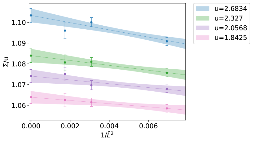
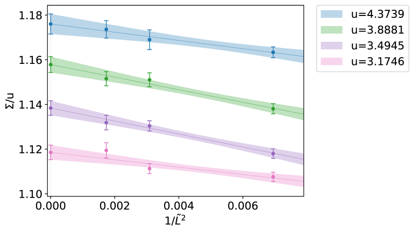
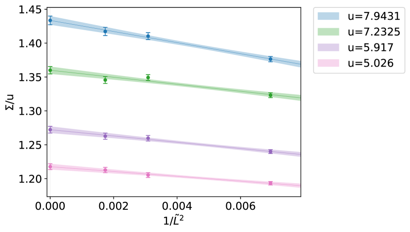
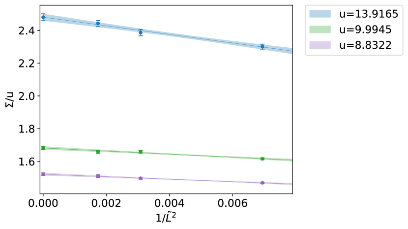
Figure 1: We display the continuum extrapolation of $\Sigma(u)/u$, performed at a few selected values of $u$.

The continuum limit of the step scaling function is obtained by performing a linear extrapolation in $1/\tilde{L}^{2}$, as illustrated in fig. 1. The continuum values of $\sigma(u)$ resulting from these fits are given in table 1. The advantage of this procedure vs the global fit presented below is that no functional dependence in $u$ is assumed for the terms representing the lattice artefacts (cf. eqs. (3.11) and (3.14)).

The resulting pairs $(u,\sigma)$ are then fitted to the series expansions given by eqs. (3.12) or (3.13), allowing to parameterize the corresponding step scaling functions in the range of couplings under consideration. For completitude we give the parameters of the fit to eq. (3.13) with $N_{c}=4$ and fitting range $\sigma\in[1.5,17]$:

$$\hat{p}_{2}=-2.86020692\times 10^{-5},\,\,\hat{p}_{3}=1.94775566\times 10^{-6},\,\,\hat{p}_{4}=-4.21570896\times 10^{-8},$$ (3.19)

and their covariance:

$$\begin{pmatrix}\,9.62610704\times 10^{-10}&-1.48907565\times 10^{-10}&\,5.49335753\times 10^{-12}\\ -1.48907565\times 10^{-10}&\,2.37337095\times 10^{-11}&-8.93899741\times 10^{-13}\\ \,5.49335753\times 10^{-12}&-8.93899741\times 10^{-13}&\,3.41858249\times 10^{-14}\end{pmatrix}\,.$$ (3.20)

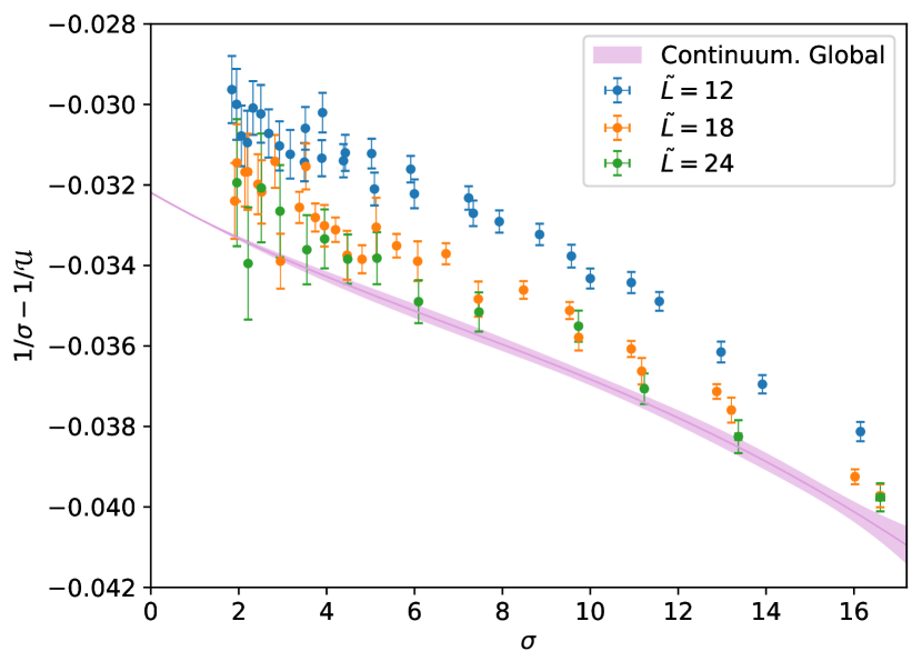
(a) Raw data for $1/\sigma-1/{\cal U}(\sigma,\tilde{L})$ vs $\sigma$.

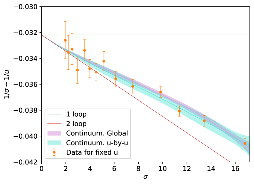
(b) Continuum extrapolation of $1/\sigma-1/u$ vs $\sigma$.

Figure 2: (a) Raw data for the inverse step scaling function compared to the continuum extrapolation obtained from the global fit, cf. eqs. (3.21), (3.22). (b) We display the comparison between various continuum extrapolations of $1/\sigma-1/u$ vs $\sigma$. The orange data points correspond to the determination at fixed values of $u$ given in table 1. The continuum extrapolations derived from the $u$-by-$u$ and the global fits described in the text, correspond respectively to the blue and pink bands, while the continuous lines indicate the perturbative predictions at order one-loop and two-loops.

3.2.2 Continuum limit from a global fit

As an alternative to the $u$-by-$u$ fit, the continuum limit can be obtained from a combined parametrization of the continuum step scaling function and a continuum extrapolation – see e.g. eq. (3.14).

From the last section, we know that the continuum step scaling function is well parametrized using three parameters in addition to the two universal terms (i.e. $N_{\rm c}=4$). Cutoff effects are well described as long as $N_{\rm l}\geq 3$, with little differences in the continuum results even if the number of parameters is increased up to $N_{\rm l}=8$. The raw data used in these fits is available in appendix B. We have fitted the data for $1/{\cal U}(\sigma,\tilde{L})$ vs $\sigma$ in the range $\sigma\in[1.5,17]$ with the particular choice $N_{\rm c}=N_{\rm l}=4$; the resulting continuum fit parameters are given by:

$$\hat{p}_{2}=-3.50622141\times 10^{-5},\,\,\hat{p}_{3}=2.14311070\times 10^{-6},\,\,\hat{p}_{4}=-2.97994910\times 10^{-8},$$ (3.21)

with covariance:

$$\begin{pmatrix}\,2.87681194\times 10^{-10}&-4.50822649\times 10^{-11}&\,1.69327683\times 10^{-12}\\ -4.50822649\times 10^{-11}&\,7.22888354\times 10^{-12}&-2.76073298\times 10^{-13}\\ \,1.69327683\times 10^{-12}&-2.76073298\times 10^{-13}&\,1.06806168\times 10^{-14}\end{pmatrix}\,.$$ (3.22)

The result of this fitting procedure is displayed in fig. 2(a) where the raw data for $1/{\cal U}(\sigma,\tilde{L})$ is represented vs $\sigma$ and compared with the continuum extrapolation resulting from this global fit which is given by the pink band displayed in the plot.

We finally present a comparison between the various continuum extrapolations in fig. 2(b). The orange points come from the direct extrapolation at fixed targeted values of $u$ given in table 1. The blue and pink bands correspond respectively to the $u$-by-$u$ and global fits described previously, showing a good agreement in all the range of fitted values. For comparison, the perturbative predictions at one and two-loop order are also shown in the figure.

3.3 Determination of $\Lambda_{\rm TGF}/\mu_{\rm had}$

The determination of $\Lambda_{\rm TGF}/\mu_{\rm had}$ relies on the use of eq. (2.8), evaluated in terms of a sequence of couplings connecting $\lambda(\mu_{\rm had})$ and $\lambda(\mu_{\rm pt})$. We have performed this sequence in two steps: an exact step connecting the coupling at scales $\mu_{\rm had}$ and $2\mu_{\rm had}$, followed by a step-scaling sequence, starting at $\lambda(2\mu_{\rm had})$, to be determined by the continuum step scaling functions obtained in the previous sections. Let us now describe these steps in detail.

$k$	TGF		MS		SF
	$\lambda(2^{k+1}\mu_{\rm had})$	$\Lambda_{\overline{\rm MS}}/(2\mu_{\rm had})$	$\lambda_{\overline{\rm MS}}(2^{k+1}\mu_{\rm had})$	$\Lambda_{\overline{\rm MS}}/(2\mu_{\rm had})$	$\lambda_{\rm SF}(0.9\times 2^{k+1}\mu_{\rm had})$	$\Lambda_{\overline{\rm MS}}/(2\mu_{\rm had})$
0	13.9164955	0.18900(10)	7.6539(49)	0.11959(18)	7.35(93)	0.207(67)
1	9.035(13)	0.19019(56)	6.3953(76)	0.14936(52)	5.934(36)	0.2263(44)
2	6.7989(88)	0.19271(71)	5.3041(72)	0.16265(80)	4.864(11)	0.2212(20)
3	5.4781(96)	0.1948(12)	4.5077(69)	0.1708(11)	4.1391(87)	0.2180(22)
4	4.5986(99)	0.1965(18)	3.9148(70)	0.1763(16)	3.6138(81)	0.2167(27)
5	3.9683(96)	0.1978(24)	3.4591(69)	0.1804(21)	3.2127(75)	0.2164(32)
6	3.4933(89)	0.1989(29)	3.0987(66)	0.1836(25)	2.8950(69)	0.2168(36)
7	3.1220(81)	0.1998(34)	2.8068(61)	0.1861(29)	2.6364(63)	0.2173(41)
8	2.8234(74)	0.2005(38)	2.5656(57)	0.1881(33)	-	-
9	2.5778(67)	0.2011(41)	2.3630(52)	0.1898(37)	-	-
10	2.3723(60)	0.2017(44)	2.1903(48)	0.1912(40)	-	-
11	2.1976(55)	0.2021(47)	2.0414(44)	0.1925(42)	-	-
12	2.0472(50)	0.2026(50)	1.9117(41)	0.1935(45)	-	-
13	1.9163(45)	0.2029(52)	1.7976(37)	0.1945(47)	-	-
14	1.8014(41)	0.2032(54)	1.6965(35)	0.1953(49)	-	-
$\infty$	0.0	0.2082(83)	0.0	0.2097(76)	0.0	0.2175(61)

Table 2: We list the couplings along the step scaling sequence starting at $\lambda(2\mu_{\rm had})=13.9164955$, corresponding to the three different computation strategies. The values of $\Lambda_{s}/(2\mu_{\rm had})$ are obtained by matching to perturbation theory at the corresponding value of $\lambda_{s}(\mu_{\rm pt})$. The final result, quoted in the last line, is obtained from a linear fit to the last 5 steps in the sequence (3 in the case of SF).

Determination of $\lambda(\mu_{\rm had})$

We fix the coupling $\lambda(2\mu_{\rm had})\equiv 13.9164955$ at values of the lattice spacing that correspond to $\tilde{L}=12,18,24$. The corresponding values of the lattice step scaling function are given in table 1, and extrapolate to a continuum value $\lambda(\mu_{\rm had})=34.52(29)$.

Determination of $\Lambda_{\overline{\rm MS}}/(2\mu_{\rm had})$

Using the fits of the continuum step scaling function, we determine a sequence of couplings $\lambda_{n}=\lambda(2^{n+1}\mu_{\rm had})$. The differences between the global and the u-by-u fits in this step are well below our statistical uncertainties. On the other hand, there are several possibilities to determine the ratio $\Lambda_{\overline{\rm MS}}/(2\mu_{\rm had})$:

TGF:

One can use the universal coefficients of the $\beta$-function and the known ratio $\Lambda_{\overline{\rm MS}}/\Lambda_{\rm TGF}$ to determine $\Lambda_{\overline{\rm MS}}/(2\mu_{\rm had})$ (cf. eq. (2.8)).

MS:

One can use the value of the ratio $\Lambda_{\overline{\rm MS}}/\Lambda_{\rm TGF}$ to determine the coupling in the $\overline{\rm MS}$ scheme as follows

$$\lambda_{\overline{\rm MS}}(2^{n+1}\mu_{\rm had})=x+2b_{0}x^{2}\log\left(\frac{\Lambda_{\overline{\rm MS}}}{\Lambda_{\rm TGF}}\right)+\mathcal{O}(x^{3})\,\qquad\left(x=\lambda\left(2^{n+1}\mu_{\rm had}\right)\right)\,.$$ (3.23)

Then, using the known 5-loop $\beta$-function [50] in the $\overline{\rm MS}$ scheme, one can determine the ratio $\Lambda_{\overline{\rm MS}}/(2\mu_{\rm had})$.

SF:

Very precise data for the SF coupling is available in reference [13]. These computations were performed at the same values of the bare coupling $b$ as our runs but on lattices of size $\tilde{L}/3$. This allows to convert non-perturbatively the values of $\lambda(2^{n+1}\mu_{\rm had})$ to values of $\lambda_{\rm SF}(0.9\times 2^{n+1}\mu_{\rm had})$. Details of this matching are available in appendix D, here it is enough to say that this matching is only possible in the region $9\gtrsim\lambda\gtrsim 3$.

After this non-perturbative conversion, the known 3-loop $\beta$-function in the SF scheme [51, 52, 53] can be used to determine the ratio $\Lambda_{\overline{\rm MS}}/(2\mu_{\rm had})$.

This procedure is similar to the approach taken in [38], and we encourage the reader interested in the details to consult that reference.

The results for the ratio $\Lambda_{\overline{\rm MS}}/(2\mu_{\rm had})$ using the different procedures described above can be seen in table 2 and in figure 3. Methods labeled TGF and MS carry a perturbative uncertainty $\mathcal{O}(\lambda(2^{n+1}\mu_{\rm had}))$ (right panel of figure 3), while the SF method carries an uncertainty $\mathcal{O}(\lambda^{2}(2^{n+1}\mu_{\rm had}))$ (left panel). Figure 3 shows that these perturbative corrections are significant in the methods labeled TGF and MS. Nevertheless the picture shows a nice agreement between all analysis methods once the limit $\lambda\to 0$ is taken.

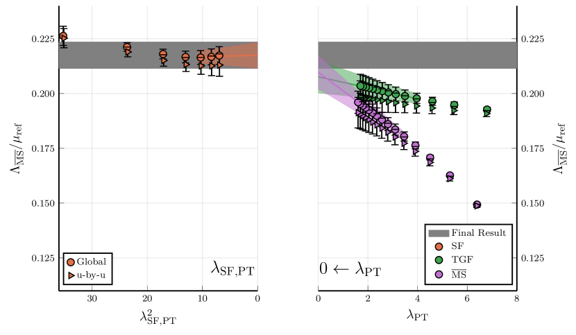
Figure 3: Ratio $\Lambda_{\overline{\rm MS}}/(2\mu_{\rm had})$ obtained through the different methods explained in the text as a function of the matching scale with perturbation theory ($\mu_{\rm ref}\equiv 2\mu_{\rm had}$). The grey band corresponds to the final result obtained from a linear fit to the 3 last steps in the SF sequence.

Finally, we quote as central value of the analysis the one labeled as SF, since it has the smallest perturbative corrections and is compatible within errors with the other two determinations. We report as final numerical value:

$$\frac{\Lambda_{\overline{\rm MS}}}{2\mu_{\rm had}}=0.2175(61)\,.$$ (3.24)

3.4 Computation of $\Lambda_{{\overline{\rm MS}}}\sqrt{8t_{0}}$

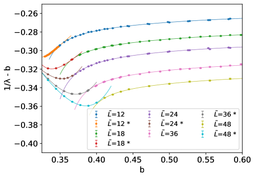
Figure 4: We display $1/\lambda-b$ as a function of $b$. The lines represent Padé fits of the form given in eq. (3.26).

$18\times b$	$t_{0}/a^{2}$	$18\times b$	$t_{0}/a^{2}$	$18\times b$	$r_{0}/a$
5.9600	2.7854(62) †	6.4200	11.241(23) †	5.7000	2.9220(90) ††
5.9600	2.7875(53) ‡	6.4500	12.196(21) ‡	5.8000	3.6730(50) ††
6.0500	3.7834(47) ‡	6.5300	15.156(28) ‡	5.9500	4.898(12) ††
6.1000	4.4329(32) ⋆	6.6100	18.714(30) ‡	6.0700	6.033(17) ††
6.1300	4.8641(85) ‡	6.6720	21.924(81) ⋆	6.1000	6.345(13) ⋆
6.1700	5.489(14) †	6.6900	23.089(48) ‡	6.2000	7.380(26) ††
6.2100	6.219(13) ‡	6.7700	28.494(66) ‡	6.3400	9.029(77) ⋆
6.2900	7.785(14) ‡	6.8500	34.819(84) ‡	6.4000	9.740(50) ††
6.3400	9.002(31) ⋆	6.9000	39.41(15) ⋆	6.5700	12.380(70) ††
6.3400	9.034(29) ⋆	6.9300	42.82(11) ‡	6.5700	12.176(97)§
6.3700	9.755(19) ‡	7.0100	52.25(13) ‡	6.6720	14.103(92) ⋆
6.4200	11.202(21) ‡			6.6900	14.20(12)§
				6.8100	16.54(12)§
				6.9000	18.93(15) ⋆
				6.9200	19.13(15)§

Table 3: Results for $t_{0}/a^{2}$ and $r_{0}/a$ for different values of $b$. For the case of $t_{0}/a^{2}$ the relevant references are ^† [20], ^‡ [54], ^⋆ [55]. For $r_{0}/a$, instead, the results are from ^†† [63] and ^⋆ [55]. The data labelled ^§ is obtained from the values of $r_{c}/a$ of [64] together with $r_{c}/r_{0}=0.5133(24)$ which gives the quoted values of $r_{0}/a$.

In order to determine the dimensionless combination $\Lambda_{{\overline{\rm MS}}}\sqrt{8t_{0}}$, we have to put together our previous results for the ratio $\Lambda_{\overline{\rm MS}}/\mu_{\rm had}$ with a determination of $\mu_{\rm had}\times\sqrt{8t_{0}}$. This quantity is computed as the continuum extrapolation of

$$\mu_{\rm had}\sqrt{8t_{0}}=\lim_{a\rightarrow 0}\,\left(a\mu_{\rm had}\times\frac{\sqrt{8t_{0}}}{a}\right).$$ (3.25)

where $a\mu_{\rm had}$ is determined by the lattice size and bare coupling for which the renormalized coupling takes the value $\lambda(\mu_{\rm had})=34.52(29)$ (see table 1). Values for $\sqrt{8t_{0}}/a$ for our choice of Wilson gauge action are available in the literature (see table 3).

Two steps were therefore required. First, for each value of $\tilde{L}$ we determined the values of the bare coupling leading to a renormalized coupling $\lambda(\mu_{\rm had})$. For this purpose, we have fitted the dependence of the coupling on $b$, at fixed $\tilde{L}$, with a Padé fit of the form:

$$b\lambda(b,\tilde{L})=\frac{a_{0}+a_{1}b+b^{2}}{a_{2}+a_{3}b+b^{2}}.$$ (3.26)

Fits are done to $1/\lambda-b$, as illustrated in fig. 4.

$\tilde{L}$	$18\times b_{\lambda=34.52}$	$a/\sqrt{8t_{0}}$	$a\mu_{\rm had}\times\sqrt{8t_{0}}/a$	$a/r_{0}$	$a\mu_{\rm had}\times r_{0}/a$
12	6.0037(26)	0.19637(96)	1.4146(69)	0.1851(20)	1.501(16)
18	6.2518(30)	0.13373(65)	1.3848(68)	0.1256(16)	1.474(18)
24	6.4574(30)	0.10029(47)	1.3848(65)	0.0947(13)	1.467(21)
36	6.7641(36)	0.06683(37)	1.3855(77)	0.0637(15)	1.453(34)
48	6.9908(30)	0.05010(25)	1.3861(70)	0.0471(39)	1.47(12)
$\infty$		0	1.3860(62)	0	1.453(19)

Table 4: Values of the bare coupling, lattice spacing and reference scales $\mu_{\rm had}\sqrt{8t_{0}}$ and $\mu_{\rm had}r_{0}$, corresponding to the renomalization condition $\lambda(\mu_{\rm had})=34.52(29)$ – see text.

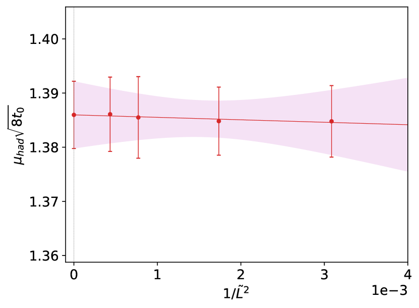
(a) $\mu_{\rm had}\times\sqrt{8t_{0}}$.

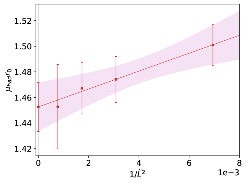
(b) $\mu_{\rm had}\times r_{0}$.

Figure 5: Continuum extrapolation of the reference scale $\mu_{\rm had}$ in units of $t_{0}$ and $r_{0}$.

After this, one has to determine $a/\sqrt{8t_{0}}$ at those values of the bare coupling. Following ref. [13], this is done by using the results quoted in refs. [20, 54, 55]. All the values for this quantity given in table 4 of ref. [13] are used to fit $\log(t_{0}/a^{2})$ to a polynomial in $b$ of degree 5 in the range $b\in[0.33,0.39]$. This fit is then used to determine $a/\sqrt{8t_{0}}$ at the specific values of the bare coupling corresponding to $\lambda(\mu_{\rm had})$ on each lattice. The results obtained from this procedure on lattices with $\tilde{L}=12$, 18, 24, 36 and 48 are given in table 4.

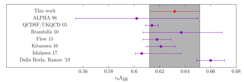
Figure 6: Final result for $r_{0}\Lambda_{{\overline{\rm MS}}}$ compared with the values included in the FLAG average [56]. These are: ALPHA 98 [57], QCDSF/UKQCD 05 [58], Brambilla [59], Flow 15 [60], Kitazawa 16 [61], Ishikawa 17 [12]. We also include the recent work Dalla Brida, Ramos 19 [13] in the comparison.

Figure 5(a) shows the continuum extrapolation of $\mu_{\rm had}\sqrt{8t_{0}}$ obtained using this strategy. We include datapoints corresponding to the $\tilde{L}=18$, 24, 36 and 48 lattices. The final continuum extrapolated value is given by:

$$\mu_{\rm had}\times\sqrt{8t_{0}}=1.3860(62).$$ (3.27)

We can now use these results to express $\Lambda_{\overline{\rm MS}}$ in units of $\sqrt{8t_{0}}$. Our final result (cf. eq. (3.24)) is:

$$\sqrt{8t_{0}}\times\Lambda_{\overline{MS}}=0.603(17).$$ (3.28)

This number is in agreement within errors with a more precise determination obtained in a recent work by one of the present authors [13]: $\sqrt{8t_{0}}\times\Lambda_{\overline{MS}}=0.6227(98)$. The strategy to obtain the $\Lambda$ parameter in that work is similar to the one presented here but is based on the use of a different gradient flow scheme with SF instead of twisted boundary conditions.

A more detailed comparison with the existing literature is better done in terms of the scale $r_{0}$ [62], which, although less precise that $t_{0}$, is used in most of the determinations of the $\Lambda$ parameter up to date. An analysis completely analogous to the one leading to eq. (3.28), allows to determine $r_{0}\times\Lambda_{\overline{\rm MS}}$. The values of $r_{0}/a$ employed in the extrapolation are shown in table 3. The values of the lattice spacing $a/r_{0}$ corresponding to the renormalization condition $\lambda(\mu_{\rm had})$ are shown in table 4 and the continuum extrapolation is displayed in fig. 5(b), leading to a value of $\mu_{\rm had}\times r_{0}=1.453(19)$. Our final result for the $\Lambda$ parameter in units of $r_{0}$ is:

$$r_{0}\times\Lambda_{\overline{\rm MS}}=0.632(20)\,.$$ (3.29)

Figure 6 shows a comparison of this result with the values included in the FLAG average [56]. With the present accuracy, our result comes out compatible with both the FLAG average $r_{0}\times\Lambda_{\overline{\rm MS}}=0.615(18)$, and the result by Dalla Brida and Ramos: $r_{0}\times\Lambda_{\overline{\rm MS}}=0.660(11)$ [13]. We believe that our particular scheme can be efficiently used to pin down the error in the determination of the $\Lambda$ parameter and clarify the tension among the existing values in the literature.

4 The effect of topology

$Q$	$\lambda(\tilde{L}=24)$	$\lambda(\tilde{L}=36)$	$\lambda(\tilde{L}=48)$
0	32.18(10)	33.29(19)	34.00(19)
1	42.92(25)	43.85(56)	43.94(49)
-1	43.07(20)	44.11(50)	-
2	$59.1^{*}$	$56.6^{*}$	-
-2	$56.4^{*}$	-	-

Table 5: Values of the TGF coupling measured on sectors with fixed value of the topological charge $Q$. Entries with a $*$ correspond to cases where the number of configurations with charge $Q$ is less than 20 and a correct estimation of errors is not viable.

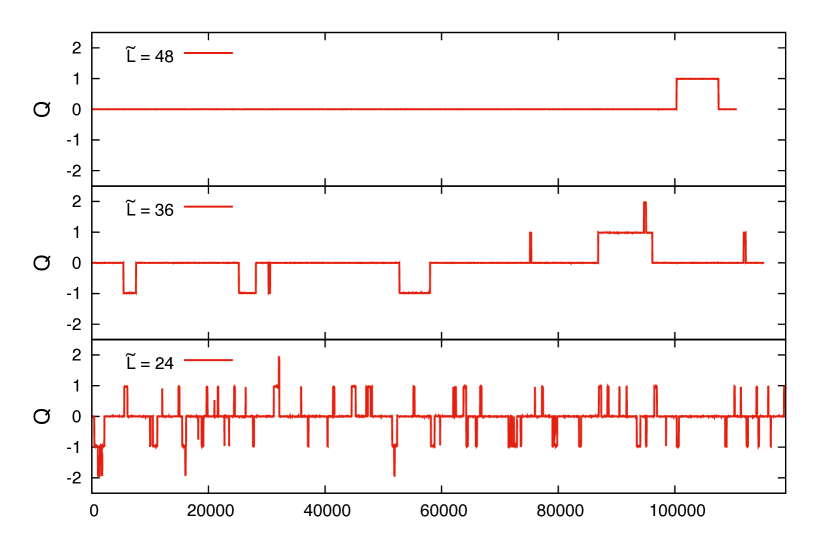
Figure 7: Topological charge vs Monte Carlo time for, from top to bottom, $\tilde{L}=48$, 36 and 24, corresponding to an approximately fixed physical size of $\tilde{l}\sim 1.1$ fm ($\lambda\sim\lambda(\mu_{\rm had})$) and to lattice spacings: $a=0.023524(96)$, $0.031141(11)$, $0.045691(92)$ fm respectively.

As explained in the introduction, our definition of the gradient flow coupling follows the prescription adopted in  [40] which amounts to evaluate the coupling in the sector of trivial topology. This choice can be seen as a particular renormalization scheme, introduced to circumvent the well known problem of toplogy freezing and critical slowing down [65]. A neat example of this effect is given in fig. 7 where we display the value of the topological charge as a function of Monte Carlo time for lattices with $\tilde{L}=24,36,48$ and a physical size corresponding to $\lambda\approx\lambda(\mu_{\rm had})$ ($\tilde{l}\sim 1.1$ fm). It is clear that our statistics in the lattices with finer lattice spacing is not enough to correctly sample the topological charge. Furthermore, as table 5 illustrates, the correlation between the coupling and the topological charge in these ensembles is very strong: values of the coupling averaged over the $Q=0$ or $|Q|=1$ sectors differ by as much as $30\%$. Clearly, when topology is poorly sampled, any attempt to compute the coupling in this volume regime by averaging over all topological sectors would lead to biased results.

In the remaning of this section we will argue that even when topology is frozen, topological charge fluctuations are correctly sampled in the trivial topology sector (see [66] for a study in the Schwinger model). We will also make an attempt to explain the observed dependence of the coupling on topology in semiclassical terms.

4.1 Topological charge fluctuations in the sector of trivial topology

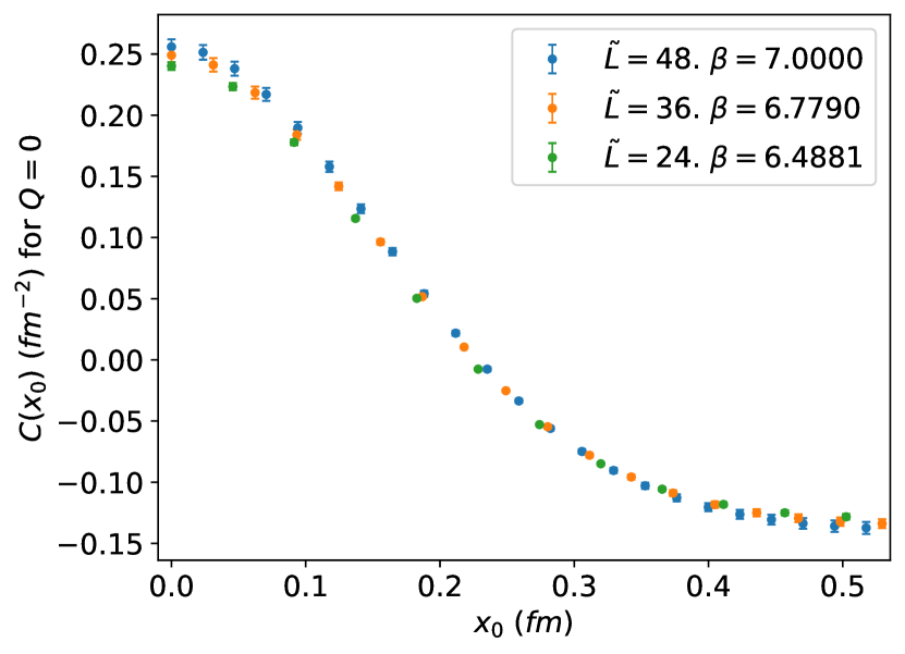
(a) $\tilde{l}\sim 1.1$ fm.

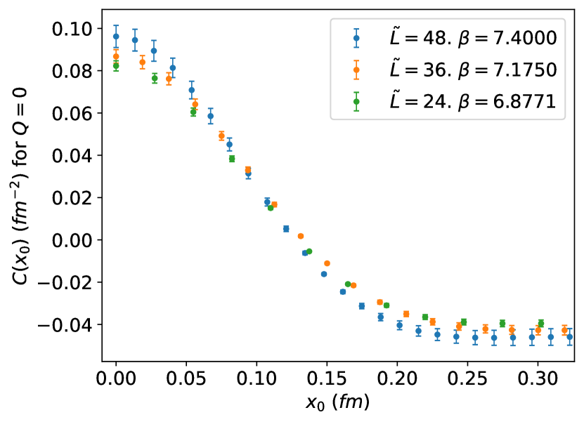
(b) $\tilde{l}\sim 0.66$ fm.

Figure 8: We display the correlator of topological charge in the trivial topology sector, defined in eq. (4.3).

In order to determine whether local fluctuations of topological charge are correctly sampled in the trivial topology sector, we have computed the two-point function of the operator:

$$q(x_{0},t)=\int d\vec{x}\,q(\vec{x},x_{0},t),$$ (4.1)

obtained by integrating the topological charge density, smeared over a flow time $t$, over three directions including the two short ones. On the lattice, this operator has been determined using the field theoretical definition of the charge density, cf. eq. (3.5),

$$q(x_{0}=n_{0}a,t)=\frac{a^{-1}}{16\pi^{2}}\sum_{\vec{n}}{\rm Tr}\left\{G^{\rm cl}_{\mu\nu}(\vec{n},n_{0},t)\widetilde{G}^{\rm cl}_{\mu\nu}(\vec{n},n_{0},t)\right\}\,,$$ (4.2)

evaluated at flow time $\sqrt{8t}=0.3\tilde{l}$. In terms of this operator, we computed the correlator:

$$C(x_{0})=\frac{\langle q(x_{0},t)\,q(0,t)\,\hat{\delta}_{Q}\rangle}{\langle\hat{\delta}_{Q}\rangle}\Big{|}_{\sqrt{8t}=0.3\tilde{l}}$$ (4.3)

defined over the sector with trivial topology.

Figure 8(a) shows the time dependence of the correlator evaluated on the Monte Carlo ensembles displayed in fig. 7. Even though topology is frozen on the largest lattice with $\tilde{L}=48$, we observe no significant deviation from scaling; the structure of the charge correlation is the same on the three lattices. These good scaling properties are independent of the physical size of the box and preserved at smaller volumes, an example for $\tilde{l}\sim 0.66$ fm is displayed in fig. 8(b). These results indicate that local fluctuations of topological charge are correctly implemented in the trivial topology sector, even when the total topological charge is frozen to zero in the Monte Carlo ensemble.

4.2 Semiclassical picture

The step scaling sequence interpolates between the perturbative domain, where non-trivial topological charge is suppressed, and the non-perturbative, strongly coupled regime. In between, in the small to intermediate volume domain, one expects semiclassical arguments based on instantons to hold. In this subsection those arguments will be used in an attempt to reproduce some of the features observed in the simulations, in particular the correlation between coupling and topological charge. By no means should this discussion be interpreted as a rigurous proof but just as a compelling qualitative picture of the role that instantons may play in this context.

In appendix E we discuss how to apply the dilute instanton gas picture to compute the leading semiclassical contribution to the TGF coupling in a fixed topological charge sector. The derivation is based on the observation that the flow removes short distance fluctuations but preserves classical solutions of the Euclidean equations of motion. This includes instantons although not instanton-anti-instanton pairs, the latter will only be preserved at typical distances larger than $\sqrt{8t}=c\tilde{l}$. The leading contribution to the TGF coupling in the semiclassical approximation can be estimated taking into account that:

$$\langle E(t)\rangle=\frac{1}{2}\langle{\rm Tr}\left(G_{\mu\nu}^{2}(x,t)\right)\rangle=\frac{1}{V}\left\langle\frac{1}{2}\int d^{4}x{\rm Tr}\left(G_{\mu\nu}^{2}(x,t)\right)\right\rangle\,.$$ (4.4)

This expression can be combined with the fact that the classical Euclidean action of a configuration with well separated instantons and anti-instantons can be approximated by $S_{0}(n+\bar{n})$, with $n(\bar{n})$ the number of instantons(anti-instantons) and $S_{0}$ the one-instanton action. Therefore, at lowest order in the dilute gas approximation, the energy density receives a (semi-)classical contribution that is proportional to the average number of instantons plus anti-instantons, i.e.,

$$\langle E(t)\rangle^{\rm dig}\sim\frac{S_{0}}{V}\,\langle n+\bar{n}\rangle+\cdots\,.$$ (4.5)

This contribution adds to the perturbative one. One can as well evaluate in this approximation the average value of any observable, in particular $\langle n+\bar{n}\rangle$, restricted to the sector of topological charge $\tilde{Q}$ by using:

$$\langle O\rangle_{\widetilde{Q}}=\frac{\langle O\,\delta_{Q-\widetilde{Q}}\rangle}{\langle\delta_{Q-\widetilde{Q}}\rangle},$$ (4.6)

with $Q$ the total topological charge, in analogy to what we did for the definition of the coupling in the zero topological sector in eq. (1.7).

In order to determine the average number of instantons in the dilute gas approximation, we have considered two possibilities: a dilute gas of ordinary instantons of action $S_{0}=8\pi^{2}$, and one made out of fractional instantons [67] with instanton action $S_{0}=8\pi^{2}/N$. The derivation follows the standard treatment, see i.e. [68]. In this context, the semiclassical picture based on the less standard case of fractional instantons follows the ideas put forward by González-Arroyo and collaborators in a series of works [69, 70, 71, 72, 73], see also [74, 75, 76].

Details of the calculation are provided in appendix  E, here we will only summarize the main final formulas. The contribution to the coupling derived in this approximation, when restricted to the sector of topological charge $Q$, reads:

$$\lambda_{Q}^{\rm dig}(c)=\frac{2NS_{0}}{3\widehat{\cal A}(\pi c^{2})}\,\left(\nu+x\,\frac{I_{\nu+1}(x)}{I_{\nu}(x)}\right)+\cdots\,,$$ (4.7)

with $\nu=Q$ for ordinary instantons, and $\nu=NQ$ for fractional ones, and where $\widehat{\cal A}(x)={\cal A}(x)/x^{2}$, coming from the coupling normalization, cf. eq. (1.7). In this expression, $I_{\nu}(x)$ stands for the modified Bessel function of the first kind, and $x=2RV$, with $R$ the probability to generate one instanton, or anti-instanton, per unit volume.

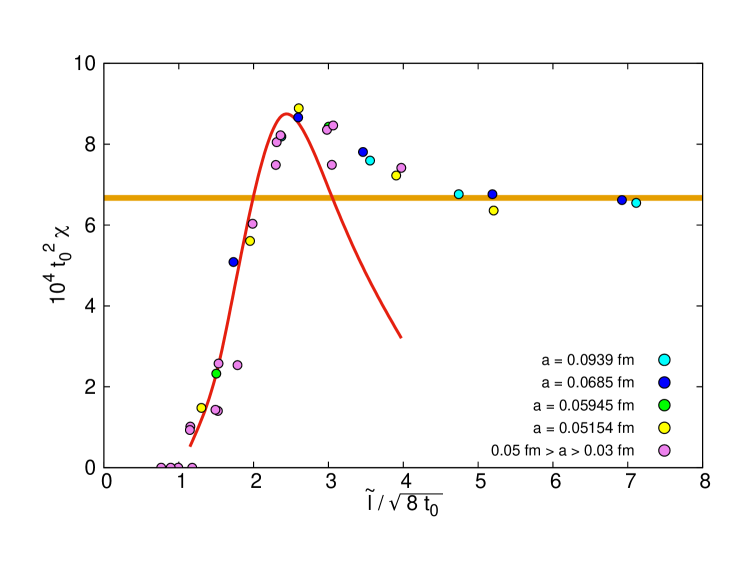
Figure 9: Volume dependence of the topological susceptibility evaluated from flowed fields at $8t=(0.3\tilde{l})^{2}$. The orange horizontal band corresponds to the value of the, continuum extrapolated, large-volume $SU(3)$ susceptibility $t_{0}^{2}\chi=6.67(7)\times 10^{-4}$ [77]. The red line gives the dilute gas estimate discussed in sec. 4.2, cf. eq. (4.11) with $C=880$.

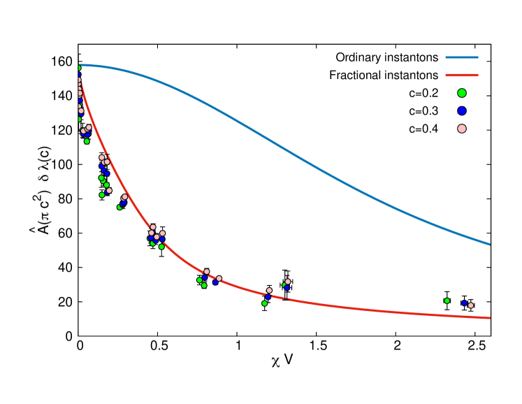
Figure 10: We display $\widehat{\cal A}(\pi c^{2})\delta\lambda(c)=\widehat{\cal A}(\pi c^{2})\left(\lambda_{Q=1}(c)-\lambda_{Q=0}(c)\right)$ as a funcion of $\chi V$ for couplings obtained at flow time $8t=(c\tilde{l})^{2}$, with $c=0,2$, 0.3 and 0.4. The lines correspond to the estimate using the leading semi-classical contribution from either fractional or ordinary instantons. Note that these lines are not fits to the data, they are directly given by eq. (4.7) with the parameter $x$ determined from the measured value of the susceptibility.

A way to determine $R$ from the numerical simulations is to measure the topological susceptibility. In the dilute gas approximation and for the case of ordinary instantons, the relation between $R$ and $\chi$ is simply given by: $\chi=2R$, while for fractional $SU(3)$ instantons one obtains instead:

$$\chi=\frac{2R}{9}\left(1-\frac{3(1+RV)}{2+e^{3RV}}\right)\,.$$ (4.8)

The topological susceptibility is defined formally in the continuum through the correlator of the topological charge density $q(x)$:

$$\chi=\int d^{4}x\left<q(x)q(0)\right>.$$ (4.9)

A proper definition requires to regulate the short-distance singularity in this expression, and this can be attained by evaluating the charge density at non-zero flow time. On the lattice, in the absence of topology freezing, the topological susceptibility can be computed by measuring:

$$\chi=\frac{\langle Q^{2}\rangle}{V}$$ (4.10)

with $Q$ the total topological charge, determined from the field theoretical definition eq. (3.7), evaluated on the flowed gauge fields.

An illustration of the volume dependence of the topological susceptibility is provided in fig. 9 where we display $t_{0}^{2}\chi$ as a function of $\tilde{l}/\sqrt{8t_{0}}$. The results shown correspond to simulations with lattice spacing $a>0.03$ fm (we refrain to give errors in this plot since our determination of the susceptibility may be affected by freezing, in particular for values of $a<0.05$ fm). The onset of the susceptibility is very abrupt and takes place for values of $\tilde{l}/\sqrt{8t_{0}}\in[1,3]$, overlapping with the region covered by the step scaling sequence. After that, $\chi$ stabilizes to the constant large volume value, given in $SU(3)$ by $t_{0}^{2}\chi=6.67(7)\times 10^{-4}$ [77], corresponding in the figure to the orange horizontal band.

By fixing $x$ in terms of the measured susceptibility, one can evaluate the dilute gas contribution to $\delta\lambda(c)=\lambda_{Q=1}(c)-\lambda_{Q=0}(c)$ and compare the result to the values of $\delta\lambda(c)$ determined in the simulations. This has been done for the set of simulations with $\beta\in[6,6.8]$ where topology seems to be properly sampled and the number of $Q=1$ configurations is sufficiently large. In addition, the calculation has been done for various values of the flow time: $8t=(c\tilde{l})^{2}$, with $c=0.2$, 0.3 and 0.4. We observe that the quantity $\widehat{\cal A}(\pi c^{2})\delta\lambda(c)$ is quite independent of the value of $c$. Our results are displayed as a function of $\chi V$ in fig. 10 and compared with the dilute gas predictions for ordinary and fractional instantons, derived from eq. (4.7). Surprisingly, the dependence predicted by the fractional instanton formula matches remarkably well our results in a large range of volumes. We stress that the lines displayed in the figure do not have any free parameter, they are directly given by eq. (4.7) with the input parameter $x$ fixed in terms of the measured value of the susceptibility.

In the dilute gas approximation one can as well obtain a prediction for the parameter $x=2RV$ in terms of the renormalized coupling. As explained in appendix E, the result for fractional instantons at one loop order reads:

$$x=2RV=C\,\frac{V}{\rho^{4}}\,\left(\lambda(1/\rho)\right)^{-2}\,e^{-8\pi^{2}/\lambda(1/\rho)}$$ (4.11)

where $\rho$ stands for the characteristic fractional instanton size, proportional to $\tilde{l}$ in the small volume regime, and $C$ for a normalization constant, unfortunately unknown. Disregarding this fact, we have used this functional form to get a qualitative idea of the volume dependence of the topological susceptibility in this approximation. The calculation requires to input the renormalized coupling constant at a scale $\rho\propto\tilde{l}$; differences in the scheme dependence translate at this order in a change of value of $C$ that depends on the ratio of $\Lambda$ parameters. We have tested the formula setting $\rho=c\tilde{l}$ and using the coupling in the TGF scheme with $c=0.2$, 0.3 and 0.4. The one with $c=0.2$ is describing better our small volume results; the red line displayed in fig. 9 corresponds to this value of $c$ and $C=880$.

To summarize, although the results presented in this section have to be taken with a grain of salt, as they are not based on a rigurous analytic calculation, we believe they provide compelling indication that some of the observed effects, in particular the correlation between topological charge and coupling, can be understood in semiclassical terms.

5 Conclusions

In this work we have investigated the running coupling using finite size scaling techniques in a scheme with twisted boundary conditions. We have used a particular choice of geometry, motivated by the study of the large $N$ limit of $SU(N)$ Yang Mills theories. In this scheme the physical size of the four dimensional volume is asymmetric, with two directions being a factor $N$ larger than the other two.

We have focused our investigations in the group $SU(3)$. For this case there are many results available in the literature, which allows for a more stringent comparison. Our determination of the $\Lambda_{\overline{\rm MS}}$ parameter in units of the flow scale $\sqrt{8t_{0}}$ or the Sommer scale $r_{0}$ shows a good agreement with the literature. The precision of our computation does not match the one of the most precise determinations, but the systematic associated with the continuum extrapolation is taken into account seriously and our simulations involve large lattices. In addition, the matching with perturbation theory is performed in several ways, using a non-perturbative running that covers large energy scales.

In this respect, it is important to note that the determination of $\Lambda_{\overline{\rm MS}}$ is accomplished in two different ways. First, we perform a direct determination in our finite volume scheme with twisted boundary conditions. In this case the ratio $\Lambda_{\overline{\rm MS}}/\Lambda_{\rm TGF}$ is a key piece in the computation. Second, we perform a non-perturbative matching with the SF coupling, using available data from the literature. The two determinations show a good agreement, but they exhibit a subtle point. The extraction of the $\Lambda$ parameter at a certain energy scale $\mu_{\rm pt}$ has perturbative corrections $\mathcal{O}(\lambda^{k}(\mu_{\rm pt}))$ (with $k=1$ in the case of the direct extraction, and $k=2$ for the case of the non-perturbative matching with the SF). A crucial point to obtain compatible results is to remove these subleading perturbative corrections by performing an extrapolation $\lambda(\mu_{\rm pt})\to 0$. At our level of precision, and specially for the case of the direct extractions, perturbative corrections are significant, even at energy scales ridiculously large.

All in all, this work shows two promising directions for future research. First, extracting the $N$ dependence of the $\Lambda$-parameter in this particular scheme is computationally cheaper than a brute force approach. Second, the particular choice of geometry shows a smaller memory footprint than usual simulations with symmetrical lattices. This smaller memory footprint implies an increase in the ratio computing over memory transfer, and therefore can be executed more efficiently in current hardware accelerators. Here it is important to stress that this pure gauge case can be non-perturbatively matched to QCD using heavy quarks [30] and has therefore direct phenomenological relevance for the extraction of the strong coupling in QCD.

The authors hope to investigate these points in detail in future works.

Appendix A Lattice ensembles

Table 6: Total number of configurations with zero topological charge (within parenthesis those with non-zero charge).

$18\times b$	$\tilde{L}=12$	$\tilde{L}=18$	$\tilde{L}=24$	$\tilde{L}=36$	$\tilde{L}=48$
6.0000	7517(2483)	20248(30694)	3920(13062)	1070(8702)	120(1876)
6.2000	9569(431)	36970(15606)	7869(10087)	1120(4159)	220(1713)
6.2980	9887(113)		5644(4356)
6.4000	9961(39)	49359(3417)	13050(5356)	3899(6983)	458(1541)
6.4881	9983(17)		8350(1650)
6.5837		9940(60)		3556(2311)
6.6000	10000(0)	52807(300)	16713(1287)	6476(4482)	759(1537)
6.6816	10000(0)		9805(195)
6.7790		10000(0)		2634(569)
6.8000	10000(0)	51840(67)	17807(193)	9593(1616)	1316(989)
6.8771	10000(0)		10000(0)
6.9769		10000(0)		4344(1615)
7.0000	10000(0)	53238(0)	16439(0)	10971(0)	2155(150)
7.0739	10000(0)		10000(0)
7.1750		10000(0)		3198(0)
7.2000	10000(0)	50544(0)	18000(0)	10974(0)	2307(0)
7.2713	10000(0)		10000(0)
7.3743		10000(0)		3231(0)
7.4000	10000(0)	53406(0)	16763(0)	10981(0)	2603(0)
7.4691	10000(0)		10000(0)
7.5735		10000(0)		3219(0)
7.6000	10000(0)	53605(0)	17760(0)	9999(0)	2308(0)
7.7734		10000(0)		3240(0)
7.8000	10000(0)	53560(0)	17501(0)	8979(0)	2604(0)
7.9663	10000(0)		10000(0)
8.0000	10000(0)	53602(0)	18000(0)	9720(0)	2610(0)
8.2721		10000(0)		3229(0)
8.4643	10000(0)		10000(0)
8.5000	10000(0)	53825(0)	17000(0)	8990(0)	2324(0)
8.7711		10000(0)		3237(0)
8.9629	10000(0)		10000(0)
9.0000	10000(0)	53654(0)	18000(0)	9000(0)	2333(0)
9.2704		10000(0)		1602(0)
9.4615	10000(0)		10000(0)
9.5000	10000(0)	54178(0)	16483(0)	7998(0)	1966(0)
9.7694		10000(0)		3255(0)
9.9609	10000(0)		10000(0)
10.0000	10000(0)	53889(0)	18000(0)	13866(0)	2898(0)
10.2686		10000(0)		8159(0)
10.4612	10000(0)		10000(0)
10.5000	10000(0)	53415(0)	17000(0)	12841(0)	2898(0)
10.7678		10000(0)		7714(0)
11.0000	10000(0)	53679(0)	8640(0)	12800(0)	2584(0)
11.4607	10000(0)		10000(0)
11.7682		10000(0)		6547(0)
12.0000	10000(0)	10000(0)	16442(0)	8916(0)	1658(0)
12.4606	10000(0)		10000(0)
12.7677		10000(0)		6550(0)
13.0000	10000(0)	10000(0)	16513(0)	8873(0)	1655(0)
13.4606	10000(0)		10000(0)
13.7673		10000(0)		5643(0)
14.0000	10000(0)	10000(0)	16340(225)	8400(0)	1663(0)
14.4612	10000(0)		10000(0)
14.7634		10000(0)		8158(0)
15.0000	10000(0)	10000(0)	16602(0)	8247(0)	1668(0)
20.0000	10000(0)	5009(0)	11570(0)	1893(0)	410(0)

Appendix B Raw data

Table 7: TGF ’t Hooft coupling data as a function of the inverse bare coupling $b=1/\lambda_{0}$ and the lattice size $\tilde{L}=\tilde{l}/a$.

$18\times b$	$\tilde{L}=12$	$\tilde{L}=18$	$\tilde{L}=24$	$\tilde{L}=36$	$\tilde{L}=48$
6.00000	34.80(11)	70.849(96)	128.69(32)	337.0(11)	656.0(51)
6.20000	21.567(67)	39.414(52)	66.69(15)	155.25(66)	310.0(22)
6.29800	17.947(52)		50.75(15)
6.40000	15.483(42)	24.809(35)	39.530(88)	84.46(24)	155.07(95)
6.48810	13.947(35)		32.18(10)
6.58370		17.892(50)		52.00(20)
6.60000	12.448(28)	17.484(22)	25.319(60)	50.06(14)	86.88(55)
6.68160	11.577(23)		21.746(70)
6.77900		13.931(34)		33.29(19)
6.80000	10.574(20)	13.585(14)	17.907(41)	31.836(90)	52.44(31)
6.87710	9.994(18)		16.148(42)
6.97690		11.573(23)		22.67(11)
7.00000	9.190(15)	11.360(10)	13.916(27)	21.603(63)	34.00(19)
7.07390	8.832(15)		12.975(30)
7.17500		10.002(18)		16.596(61)
7.20000	8.243(13)	9.8366(80)	11.571(17)	16.023(43)	22.78(16)
7.27130	7.943(12)		10.933(21)
7.37430		8.826(15)		13.210(43)
7.40000	7.444(11)	8.7118(62)	9.999(14)	12.878(27)	16.599(89)
7.46910	7.232(11)		9.570(17)
7.57350		7.927(12)		11.170(33)
7.60000	6.836(11)	7.8398(53)	8.846(11)	10.931(21)	13.370(68)
7.77340		7.220(11)		9.736(24)
7.80000	6.2882(91)	7.1400(47)	7.9290(95)	9.530(17)	11.229(44)
7.96630	5.9170(84)		7.337(11)
8.00000	5.8619(84)	6.5569(42)	7.2322(83)	8.482(14)	9.731(33)
8.27210		5.9161(85)		7.452(20)
8.46430	5.0260(68)		5.9971(85)
8.50000	4.9827(67)	5.4767(33)	5.9142(66)	6.717(11)	7.467(25)
8.77110		5.0356(69)		6.072(15)
8.96290	4.3739(59)		5.0883(70)
9.00000	4.3426(57)	4.7096(28)	5.0237(51)	5.5922(83)	6.092(18)
9.27040		4.3850(59)		5.128(17)
9.46150	3.8881(51)		4.4249(59)
9.50000	3.8529(50)	4.1335(23)	4.3831(46)	4.8058(74)	5.146(16)
9.76940		3.8813(51)		4.466(10)
9.96090	3.4945(44)		3.9068(51)
10.0000	3.4676(44)	3.6895(20)	3.8903(38)	4.2029(47)	4.480(11)
10.2686		3.4943(45)		3.9500(57)
10.4612	3.1746(40)		3.5160(44)
10.5000	3.1481(38)	3.3331(18)	3.4938(34)	3.7424(43)	3.954(11)
10.7678		3.1747(39)		3.5280(52)
11.0000	2.8860(36)	3.0458(17)	3.1720(42)	3.3810(40)	3.5505(94)
11.4607	2.6834(32)		2.9271(36)
11.7682		2.6817(32)		2.9499(45)
12.0000	2.4778(30)	2.5955(32)	2.6819(26)	2.8259(36)	2.9393(94)
12.4606	2.3270(28)		2.5031(31)
12.7677		2.3320(28)		2.5211(38)
13.0000	2.1738(25)	2.2608(27)	2.3259(22)	2.4370(31)	2.5134(82)
13.4606	2.0568(24)		2.1967(26)
13.7673		2.0601(25)		2.2038(36)
14.0000	1.9357(23)	2.0069(23)	2.0584(19)	2.1432(28)	2.2130(65)
14.4612	1.8425(21)		1.9503(23)
14.7634		1.8449(22)		1.9585(27)
15.0000	1.7483(20)	1.7971(21)	1.8439(17)	1.9082(25)	1.9593(57)
20.0000	1.1748(13)	1.1988(20)	1.2137(13)	1.2440(32)	1.2705(68)

Appendix C Continuum extrapolation for the step scaling function

Table 8: Raw data for the lattice step scaling function $\Sigma(u)$ at the values of $u$ tuned for the $u$-by-$u$ continuum extrapolation - see sec. 3.2.1. The small mismatch in fixing the value of $u$ is corrected for by slightly shifting the lattice step scaling functions to a constant value $u_{\text{tg}}$, leading to the values $\Sigma(u_{\text{tg}})$ given in the table. We also give the continuum step scaling function obtained from the continuum extrapolations displayed in fig. 1.

$\tilde{L}$	$18\times b$	$u$	$\Sigma(u)$	$\Sigma(u_{\rm tg})$
12	14.4612	1.8425(21)	1.9503(23)	1.9503(34)
18	14.7634	1.8449(22)	1.9566(40)	1.9558(37)
24	15.0000	1.8439(17)	1.9593(58)	1.9577(61)
$\infty$		$u_{\rm tg}=$1.8425		1.9602(55)
12	13.4606	2.0568(23)	2.1967(26)	2.1967(38)
18	13.7630	2.0601(25)	2.2038(35)	2.2002(46)
24	14.0000	2.0584(19)	2.2130(64)	2.2113(68)
$\infty$		$u_{\rm tg}=$2.0568		2.2092(65)
12	12.4606	2.3270(28)	2.5031(31)	2.5031(45)
18	12.7677	2.3320(28)	2.5211(38)	2.5153(50)
24	13.0000	2.3259(22)	2.5134(81)	2.5147(85)
$\infty$		$u_{\rm tg}=$2.3270		2.5224(75)
12	11.4607	2.6834(32)	2.9271(36)	2.9271(52)
18	11.7682	2.6817(32)	2.9498(44)	2.9519(59)
24	12.0000	2.6819(26)	2.9393(93)	2.9411(99)
$\infty$		$u_{\rm tg}=$2.6834		2.9607(88)
12	10.4612	3.1746(40)	3.5160(44)	3.5160(66)
18	10.7678	3.1747(39)	3.5280(52)	3.5278(71)
24	11.0000	3.1720(42)	3.5505(94)	3.554(11)
$\infty$		$u_{\rm tg}=$3.1746		3.555(10)
12	9.96090	3.4945(44)	3.9068(51)	3.9068(75)
18	10.2686	3.4943(45)	3.9500(57)	3.9502(81)
24	10.5000	3.4938(34)	3.954(11)	3.955(11)
$\infty$		$u_{\rm tg}=$3.4945		3.978(11)
12	9.46150	3.8881(50)	4.4249(59)	4.4249(88)
18	9.76940	3.8813(51)	4.466(10)	4.475(12)
24	10.0000	3.8903(38)	4.480(11)	4.477(12)
$\infty$		$u_{\rm tg}=$3.8881		4.501(14)
12	8.96290	4.3739(59)	5.0883(70)	5.088(11)
18	9.27040	4.3850(59)	5.128(17)	5.113(19)
24	9.50000	4.3831(46)	5.146(16)	5.133(17)
$\infty$		$u_{\rm tg}=$4.3739		5.143(20)
12	8.46430	5.0260(68)	5.9971(85)	5.997(13)
18	8.77110	5.0356(69)	6.072(15)	6.058(18)
24	9.00000	5.0237(51)	6.092(18)	6.095(20)
$\infty$		$u_{\rm tg}=$5.0260		6.120(22)
12	7.96630	5.9170(84)	7.337(11)	7.337(17)
18	8.27210	5.9161(85)	7.452(20)	7.453(24)
24	8.50000	5.9142(66)	7.467(25)	7.471(27)
$\infty$		$u_{\rm tg}=$5.9170		7.527(29)
12	7.46910	7.232(11)	9.570(17)	9.570(26)
18	7.77340	7.220(11)	9.726(31)	9.758(31)
24	8.00000	7.2322(83)	9.734(36)	9.732(37)
$\infty$		$u_{\rm tg}=$7.2325		9.836(39)
12	7.27130	7.943(12)	10.933(21)	10.933(31)
18	7.57350	7.927(12)	11.163(41)	11.202(41)
24	7.80000	7.9290(95)	11.210(47)	11.257(48)
$\infty$		$u_{\rm tg}=$7.9431		11.386(51)
12	7.07390	8.832(15)	12.975(30)	12.975(44)
18	7.37430	8.826(15)	13.185(52)	13.223(54)
24	7.60000	8.846(11)	13.370(68)	13.339(73)
$\infty$		$u_{\rm tg}=$8.8322		13.434(71)
12	6.87710	9.994(18)	16.148(42)	16.148(63)
18	7.17500	10.002(18)	16.596(61)	16.575(78)
24	7.40000	9.999(14)	16.599(89)	16.585(96)
$\infty$		$u_{\rm tg}=$9.9945		16.81(10)
12	6.48810	13.947(35)	32.17(11)	32.01(21)
18	6.77900	13.931(34)	33.29(20)	33.21(27)
24	7.00000	13.916(27)	34.00(20)	34.00(25)
$\infty$		$u_{\rm tg}=$13.91650		34.52(29)

Appendix D Matching with the SF scheme

In order to match the values of the coupling $\lambda_{\rm TGF}(\mu)$ to the SF scheme, we use a set of simulations performed at the same values of the bare coupling but on a symmetric lattice with size $L_{\rm SF}=\tilde{L}/3$ with SF boundary conditions and an abelian background field [31]. The values of the SF coupling in these simulations can be checked in reference [13] .

We perform a fit, discarding the SF data with $\tilde{L}=18$, of the form

$$\frac{1}{\lambda_{\rm SF}(\mu)}-\frac{1}{u}=\sum_{n=0}^{N_{l}}c_{k}u^{k}+\left(\frac{1}{\tilde{L}^{2}}\right)\times\sum_{n=0}^{8}\rho_{k}u^{k}\,,$$ (D.1)

where $c_{k}$ are the fit coefficients and

$$u=\lambda_{\rm TGF}(\mu/0.9)\,.$$ (D.2)

The result of the fit can be seen in Figure 11. This fit can only be trusted for $3<\lambda_{\rm TGF}<6$, since data on the SF scheme at higher energies is not available in the literature.

Figure 11: Non perturbative matching between the SF and the TGF couplings. We use the available data for the SF coupling in [13]. In the fit we discard the data with $\tilde{L}=18$, but these are plotted to show the consistency of the fit.

Appendix E Dilute gas approximation

In this appendix we present the derivation of the dependence of the coupling on the topological charge in the dilute gas approximation. The starting point is the continuum expression for the TGF coupling:

$$\lambda(\mu)=\frac{128\pi^{2}t^{2}}{3N{\cal A}(\pi c^{2})}\langle E\left(t\right)\rangle\Big{|}_{\sqrt{8t}=c\tilde{l}=\mu^{-1}}\,.$$ (E.1)

By setting ${\cal A}(x)=x^{2}\widehat{\cal A}(x)$, and $(8t)^{2}=c^{4}\tilde{l}^{4}=c^{4}N^{2}V$, with $V$ the volume of the asymmetric box, one gets:

$$\lambda(\mu)=\frac{2NV}{3\widehat{{\cal A}}(\pi c^{2})}\langle E(t)\rangle\Big{|}_{\sqrt{8t}=c\tilde{l}=\mu^{-1}}\,.$$ (E.2)

We will use that:

$$\langle E(t)\rangle=\frac{1}{2}\langle{\rm Tr}\left(G_{\mu\nu}^{2}(x,t)\right)\rangle=\frac{1}{2V}\left\langle\int d^{4}x\,{\rm Tr}\left(G_{\mu\nu}^{2}(x,t)\right)\right\rangle_{Q}\,.$$ (E.3)

In a configuration with well separated instantons and anti-instantons, the classical Euclidean action can be approximated by $S_{0}(n+\overline{n})$, with $S_{0}$ the one-instanton action and $n(\overline{n})$ the number of instantons(anti-instantons). Therefore, one can compute the contribution to the expectation value of the energy density at leading order in this approximation by estimating the average number of instantons plus anti-instantons in the flowed ensemble:

$$\langle E(t)\rangle^{\rm dig}\sim\frac{S_{0}}{V}\,\langle n+\overline{n}\rangle\,.$$ (E.4)

Here we rely on the assumption that the flow removes short distance fluctuations but preserves instantons, note though that this is not the case for instanton-anti-instanton pairs which will only be preserved at distances larger than $\sqrt{8t}=c\tilde{l}$.

Finally, the evaluation of the coupling can be restricted to sectors of definite topological charge $Q$, cf. eq. (4.6), leading to:

$$\lambda_{Q}^{\rm dig}(c)\sim\frac{2NS_{0}}{3\widehat{\cal A}(\pi c^{2})}\,\langle n+\overline{n}\rangle_{Q}\,.$$ (E.5)

In the remaining of this section we will determine the expectation value of $n+\overline{n}$ considering two different scenarios, a dilute gas of ordinary instantons with $S_{0}=8\pi^{2}$, and one made of fractional instantons of action $S_{0}=8\pi^{2}/N$.

E.1 Ordinary instantons

The basic asumption in the dilute gas approximation is that the gas is made of objects with positive (+1) and negative (-1) topological charge that are otherwise equally probable; the probality to create either of them per unit volume is given by $R$. Under this hypothesis, it is easy to determine the partition function restricted to the sector of topological charge $Q$, it is given by:

$$Z_{Q}={\cal C}\sum_{n,\overline{n}}\frac{1}{n!\overline{n}!}(RV)^{n+\overline{n}}\delta(n-\overline{n}-Q)={\cal C}\int_{0}^{2\pi}\frac{d\theta}{2\pi}e^{-iQ\theta}\exp\{2RV\cos\theta\}={\cal C}I_{Q}(2RV)\,,$$ (E.6)

where we have used the integral representation of the $\delta$ function:

$$\delta(x)=\frac{1}{2\pi}\int_{0}^{2\pi}d\theta e^{i\theta x}\,,$$ (E.7)

and where $I_{Q}(x)$ stands for the modified Bessel function of the first kind. It is easy to evaluate $\langle n+\overline{n}\rangle_{Q}$ in this approximation, it is given by:

$$\langle n+\overline{n}\rangle_{Q}=\frac{\partial\log I_{Q}(x)}{\partial\log x}=x\left(\frac{I_{Q-1}(x)+I_{Q+1}(x)}{2I_{Q}(x)}\right)=Q+x\,\frac{I_{Q+1}(x)}{I_{Q}(x)}\,,$$ (E.8)

where $x=2RV$.

We can also compute the topological susceptibility in this approximation. The partition function in the $\theta$ vacuum is given by:

$$Z(\theta)={\cal C}\sum_{n,\overline{n}}\frac{1}{n!\overline{n}!}(RV)^{n+\overline{n}}e^{i(n-\overline{n})\theta}={\cal C}e^{2RV\cos\theta}\,,$$ (E.9)

and the topological susceptibility can be computed from:

$$\chi=\left\langle\frac{(n-\overline{n})^{2}}{V}\right\rangle=-\frac{1}{VZ(\theta)}\frac{\partial^{2}Z(\theta)}{\partial^{2}\theta}\Big{|}_{\theta=0}=2R\,.$$ (E.10)

In the dilute gas approximation $R$ is determined from the determinant of the fluctuation operator around one instanton. The result at one-loop order in infinite volume reads

$$R=A\,\left(\lambda(\mu)\right)^{-\frac{n_{c}}{2}}\,e^{-NS_{0}/\lambda(\mu)}\int_{0}^{\infty}\frac{d\rho}{\rho^{5}}\,(\rho\mu)^{2Nb_{0}S_{0}}\,,$$ (E.11)

where $n_{c}$ is the number of collective coordinates, equalt to $4N$ for ordinary $SU(N)$ instantons. The formula up to two loops including the prefactor has been computed in ref. [78]. The resulting expression is infrared divergent, although on a finite volume it would be cutoff by the size of the box. Note however, that for the determination of $\lambda_{Q}^{\rm dig}$ we only need the relation $x=2RV=\chi V$, where one can use the measured topological susceptibility to determine the input parameter $x$ and evaluate the coupling using eq. (E.8).

E.2 Fractional instantons

In the case of fractional instantons, the only difference stems from the fact that instantons contribute with charge $\pm 1/N$ to the partition function. Note that the twist used in our simulations is in the class of the so-call orthogonal twists, satisfying $n_{\mu\nu}\tilde{n}_{\mu\nu}/4=0$ (mod $N$) and therefore the total topological charge is still quantized in integer units. This fact has to be taken into account when formulating the dilute gas partition function for fractional instantons and therefore:

$$Z_{Q}={\cal C}\sum_{n,\overline{n}}\frac{1}{n!\overline{n}!}(RV)^{n+\overline{n}}\delta(n-\overline{n}-NQ)\,.$$ (E.12)

We can now use that:

$$I_{\alpha}(x)=\sum_{n}\frac{1}{n!\Gamma(n+\alpha+1)}\left(\frac{x}{2}\right)^{2n+\alpha}\,,$$ (E.13)

to obtain ($x=2RV$):

$$Z_{Q}={\cal C}I_{NQ}(x)\,,$$ (E.14)

and

$$\langle n+\overline{n}\rangle_{Q}=x\,\left(\frac{I_{NQ-1}(x)+I_{NQ+1}(x)}{2I_{NQ}(x)}\right)=NQ+x\,\frac{I_{NQ+1}(x)}{I_{NQ}(x)}\,.$$ (E.15)

As for the topological susceptibility, using:

$$Z(\theta)=\sum_{Q\in\mathbf{Z}}e^{iQ\theta}Z_{Q}\,,$$ (E.16)

and the following representation for the Kronecker delta function:

$$\delta(n-\overline{n}-NQ)=\frac{1}{N}\sum_{k=1}^{N}e^{2\pi i\frac{k}{N}(n-\overline{n})}\,,$$ (E.17)

one arrives at:

$$Z(\theta)=\frac{{\cal C}}{N}\sum_{k=1}^{N}\exp\left\{x\cos\left(\frac{\theta+2\pi k}{N}\right)\right\}\,,$$ (E.18)

leading to the following expression for the $N=3$ topological susceptibility:

$$\chi=\frac{x}{18V}\,\left(2-\frac{3(2+x)}{2+e^{3x/2}}\right)\,.\,.$$ (E.19)

The relation between $x=2RV$ and $\chi V$ is more involved in this case than for ordinary instantons, but nevertheless it can be numerically inverted to obtain $x$ in terms of $\chi V$.

In the dilute gas approximation, see i.e. [69, 70]:

$$R=\widehat{C}\,\left(\lambda(\mu)\right)^{-2}\,e^{-NS_{0}/\lambda(\mu)}\frac{1}{\rho^{4}}\,(\rho\mu)^{2Nb_{0}S_{0}}\,,$$ (E.20)

where $\rho$ is the characteristic fractional instanton size. The peculiarity of fractional instantons vs ordinary ones is that the collective coordinates only include the instanton location; in particular the size is not a moduli parameter and on a finite volume it is fixed in terms of the volume of the box. Therefore, we expect $\rho\propto\tilde{l}$ in the small volume regime and $\rho\propto 1/\Lambda_{QCD}$ for large volumes. When $\rho\propto\tilde{l}$, and setting $\mu=1/(c\tilde{l})$, we can write:

$$x=2RV=C\frac{V}{(c\tilde{l})^{4}}\,\left(\lambda(\mu)\right)^{-2}\,e^{-8\pi^{2}/\lambda(\mu)}\Big{|}_{\mu=(c\tilde{l})^{-1}}\,,$$ (E.21)

and determine $x$, up to an overall normalization constant, from the measurement of the TGF coupling.

References

- [1] M. Lüscher, P. Weisz, and U. Wolff, “A Numerical method to compute the running coupling in asymptotically free theories,” Nucl.Phys. B359 (1991) 221–243.
- [2] M. Luscher, “Advanced lattice QCD,” in Les Houches Summer School in Theoretical Physics, Session 68: Probing the Standard Model of Particle Interactions. 2, 1998. arXiv:hep-lat/9802029.
- [3] R. Sommer, “Non-perturbative renormalization of QCD,” arXiv:hep-ph/9711243 [hep-ph].
- [4] H. D. Politzer, “Reliable Perturbative Results for Strong Interactions?,” Phys. Rev. Lett. 30 (1973) 1346–1349. [,274(1973)].
- [5] D. J. Gross and F. Wilczek, “Ultraviolet Behavior of Nonabelian Gauge Theories,” Phys. Rev. Lett. 30 (1973) 1343–1346. [,271(1973)].
- [6] L. Del Debbio and A. Ramos, “Lattice determinations of the strong coupling,” arXiv:2101.04762 [hep-lat].
- [7] PACS-CS Collaboration, S. Aoki et al., “Precise determination of the strong coupling constant in lattice QCD with the Schrödinger functional scheme,” JHEP 0910 (2009) 053, arXiv:0906.3906 [hep-lat].
- [8] ALPHA Collaboration, M. Dalla Brida, P. Fritzsch, T. Korzec, A. Ramos, S. Sint, and R. Sommer, “Slow running of the Gradient Flow coupling from 200 MeV to 4 GeV in QCD,” Phys. Rev. D95 no. 1, (2017) 014507, arXiv:1607.06423 [hep-lat].
- [9] ALPHA Collaboration, M. Bruno, M. Dalla Brida, P. Fritzsch, T. Korzec, A. Ramos, S. Schaefer, H. Simma, S. Sint, and R. Sommer, “QCD Coupling from a Nonperturbative Determination of the Three-Flavor Parameter,” Phys. Rev. Lett. 119 no. 10, (2017) 102001, arXiv:1706.03821 [hep-lat].
- [10] ALPHA Collaboration, F. Tekin, R. Sommer, and U. Wolff, “The running coupling of QCD with four flavors,” Nucl.Phys. B840 (2010) 114–128, arXiv:1006.0672 [hep-lat].
- [11] M. Lüscher, R. Sommer, P. Weisz, and U. Wolff, “A precise determination of the running coupling in the SU(3) Yang-Mills theory,” Nucl.Phys. B413 (1994) 481–502, arXiv:hep-lat/9309005 [hep-lat].
- [12] K.-I. Ishikawa, I. Kanamori, Y. Murakami, A. Nakamura, M. Okawa, and R. Ueno, “Non-perturbative determination of the -parameter in the pure SU(3) gauge theory from the twisted gradient flow coupling,” JHEP 12 (2017) 067, arXiv:1702.06289 [hep-lat].
- [13] M. Dalla Brida and A. Ramos, “The gradient flow coupling at high-energy and the scale of SU(3) Yang-Mills theory,” arXiv:1905.05147 [hep-lat].
- [14] E. I. Bribian and M. Garcia Perez, “The twisted gradient flow coupling at one loop,” arXiv:1903.08029 [hep-lat].
- [15] E. I. Bribian, M. Garcia Perez, and A. Ramos, “The twisted gradient flow running coupling in SU(3): a non-perturbative determination,” in 37th International Symposium on Lattice Field Theory (Lattice 2019) Wuhan, Hubei, China, June 16-22, 2019. 2020. arXiv:2001.03735 [hep-lat].
- [16] E. Ibañez Bribián, Volume (in)dependence in Yang-Mills theories. PhD thesis, Madrid, Autonoma U., 2019.
- [17] R. Narayanan and H. Neuberger, “Infinite N phase transitions in continuum Wilson loop operators,” JHEP 0603 (2006) 064, arXiv:hep-th/0601210 [hep-th].
- [18] R. Lohmayer and H. Neuberger, “Continuous smearing of Wilson Loops,” PoS LATTICE2011 (2011) 249, arXiv:1110.3522 [hep-lat].
- [19] M. Lüscher, “Trivializing maps, the Wilson flow and the HMC algorithm,” Commun.Math.Phys. 293 (2010) 899–919, arXiv:0907.5491 [hep-lat].
- [20] M. Lüscher, “Properties and uses of the Wilson flow in lattice QCD,” JHEP 1008 (2010) 071, arXiv:1006.4518 [hep-lat].
- [21] A. Ramos, “The Yang-Mills gradient flow and renormalization,” PoS LATTICE2014 (2015) 017, arXiv:1506.00118 [hep-lat].
- [22] G. ’t Hooft, “A Property of Electric and Magnetic Flux in Nonabelian Gauge Theories,” Nucl. Phys. B 153 (1979) 141–160.
- [23] G. ’t Hooft, “Confinement and Topology in Nonabelian Gauge Theories,” Acta Phys. Austriaca Suppl. 22 (1980) 531–586.
- [24] G. ’t Hooft, “Aspects of Quark Confinement,” Phys. Scripta 24 (1981) 841–846.
- [25] A. Gonzalez-Arroyo and M. Okawa, “The Twisted Eguchi-Kawai Model: A Reduced Model for Large N Lattice Gauge Theory,” Phys.Rev. D27 (1983) 2397.
- [26] A. Gonzalez-Arroyo and M. Okawa, “A Twisted Model for Large Lattice Gauge Theory,” Phys.Lett. B120 (1983) 174.
- [27] A. Gonzalez-Arroyo and M. Okawa, “Large reduction with the Twisted Eguchi-Kawai model,” JHEP 1007 (2010) 043, arXiv:1005.1981 [hep-th].
- [28] M. G. Perez, A. Gonzalez-Arroyo, and M. Okawa, “Volume independence for Yang-Mills fields on the twisted torus,” arXiv:1406.5655 [hep-th].
- [29] M. García Pérez, “Prospects for large N gauge theories on the lattice,” PoS LATTICE2019 (2020) 276, arXiv:2001.10859 [hep-lat].
- [30] ALPHA Collaboration, M. Dalla Brida, R. Höllwieser, F. Knechtli, T. Korzec, A. Ramos, and R. Sommer, “Non-perturbative renormalization by decoupling,” Phys. Lett. B 807 (2020) 135571, arXiv:1912.06001 [hep-lat].
- [31] M. Lüscher, R. Narayanan, P. Weisz, and U. Wolff, “The Schrödinger Functional: a renormalizable probe for non-abelian gauge theories,” Nucl.Phys. B384 (1992) 168–228, arXiv:hep-lat/9207009 [hep-lat].
- [32] P. Fritzsch and A. Ramos, “The gradient flow coupling in the Schrödinger Functional,” JHEP 1310 (2013) 008, arXiv:1301.4388 [hep-lat].
- [33] M. Lüscher, “Step scaling and the Yang-Mills gradient flow,” JHEP 1406 (2014) 105, arXiv:1404.5930 [hep-lat].
- [34] A. Ramos, “The gradient flow running coupling with twisted boundary conditions,” JHEP 1411 (2014) 101, arXiv:1409.1445 [hep-lat].
- [35] L. Keegan and A. Ramos, “(Dimensional) twisted reduction in large N gauge theories,” in Proceedings, 33rd International Symposium on Lattice Field Theory (Lattice 2015). 2015. arXiv:1510.08360 [hep-lat]. https://inspirehep.net/record/1401229/files/arXiv:1510.08360.pdf.
- [36] Z. Fodor, K. Holland, J. Kuti, D. Nogradi, and C. H. Wong, “The Yang-Mills gradient flow in finite volume,” JHEP 1211 (2012) 007, arXiv:1208.1051 [hep-lat].
- [37] Z. Fodor, K. Holland, J. Kuti, D. Nogradi, and C. H. Wong, “The gradient flow running coupling scheme,” arXiv:1211.3247 [hep-lat].
- [38] A. Nada and A. Ramos, “An analysis of systematic effects in finite size scaling studies using the gradient flow,” Eur. Phys. J. C 81 no. 1, (2021) 1, arXiv:2007.12862 [hep-lat].
- [39] L. Del Debbio, G. M. Manca, and E. Vicari, “Critical slowing down of topological modes,” Phys.Lett. B594 (2004) 315–323, arXiv:hep-lat/0403001 [hep-lat].
- [40] P. Fritzsch, A. Ramos, and F. Stollenwerk, “Critical slowing down and the gradient flow coupling in the Schrödinger functional,” PoS Lattice2013 (2013) 461, arXiv:1311.7304 [hep-lat].
- [41] M. Lüscher and P. Weisz, “Perturbative analysis of the gradient flow in non-abelian gauge theories,” JHEP 1102 (2011) 051, arXiv:1101.0963 [hep-th].
- [42] F. Chamizo and A. Gonzalez-Arroyo, “Tachyonic instabilities in 2 + 1 dimensional Yang–Mills theory and its connection to number theory,” J. Phys. A 50 no. 26, (2017) 265401, arXiv:1610.07972 [hep-th].
- [43] M. García Pérez, A. González-Arroyo, M. Koren, and M. Okawa, “The spectrum of 2+1 dimensional Yang-Mills theory on a twisted spatial torus,” JHEP 07 (2018) 169, arXiv:1807.03481 [hep-th].
- [44] M. García Pérez, A. González-Arroyo, and M. Okawa, “Spatial volume dependence for 2+1 dimensional SU(N) Yang-Mills theory,” JHEP 1309 (2013) 003, arXiv:1307.5254 [hep-lat].
- [45] U. Wolff, “Dynamics of hybrid overrelaxation in the Gaussian model,” Phys.Lett. B288 (1992) 166–170.
- [46] M. Creutz, “Monte Carlo Study of Quantized SU(2) Gauge Theory,” Phys.Rev. D21 (1980) 2308–2315.
- [47] K. Fabricius and O. Haan, “Heat Bath Method for the Twisted Eguchi-Kawai Model,” Phys.Lett. B143 (1984) 459.
- [48] M. Creutz, “Overrelaxation and Monte Carlo Simulation,” Phys.Rev. D36 (1987) 515.
- [49] N. Husung, P. Marquard, and R. Sommer, “Asymptotic behavior of cutoff effects in Yang-Mills theory and in Wilson’s lattice QCD,” arXiv:1912.08498 [hep-lat].
- [50] P. A. Baikov, K. G. Chetyrkin, and J. H. Kḧn, “Five-Loop Running of the QCD coupling constant,” Phys. Rev. Lett. 118 no. 8, (2017) 082002, arXiv:1606.08659 [hep-ph].
- [51] Alpha Collaboration, A. Bode, U. Wolff, and P. Weisz, “Two loop computation of the Schrodinger functional in pure SU(3) lattice gauge theory,” Nucl. Phys. B540 (1999) 491–499, arXiv:hep-lat/9809175 [hep-lat].
- [52] A. Bode, P. Weisz, and U. Wolff, “Two loop lattice expansion of the Schrodinger functional coupling in improved QCD,” Nucl. Phys. Proc. Suppl. 83 (2000) 920–922, arXiv:hep-lat/9908044 [hep-lat].
- [53] ALPHA Collaboration, A. Bode, P. Weisz, and U. Wolff, “Two loop computation of the Schrodinger functional in lattice QCD,” Nucl. Phys. B576 (2000) 517–539, arXiv:hep-lat/9911018 [hep-lat]. [Erratum: Nucl. Phys.B600,453(2001)].
- [54] Giusti, Leonardo and Lüscher, Martin, “Topological susceptibility at from master-field simulations of the SU(3) gauge theory,” arXiv:1812.02062 [hep-lat].
- [55] ALPHA Collaboration, F. Knechtli, T. Korzec, B. Leder, and G. Moir, “Power corrections from decoupling of the charm quark,” Phys. Lett. B774 (2017) 649–655, arXiv:1706.04982 [hep-lat].
- [56] Flavour Lattice Averaging Group Collaboration, S. Aoki et al., “FLAG Review 2019,” arXiv:1902.08191 [hep-lat].
- [57] ALPHA Collaboration, S. Capitani, M. Lüscher, R. Sommer, and H. Wittig, “Non-perturbative quark mass renormalization in quenched lattice QCD,” Nucl.Phys. B544 (1999) 669–698, arXiv:hep-lat/9810063 [hep-lat].
- [58] M. Gockeler, R. Horsley, A. C. Irving, D. Pleiter, P. E. L. Rakow, G. Schierholz, and H. Stuben, “A Determination of the Lambda parameter from full lattice QCD,” Phys. Rev. D73 (2006) 014513, arXiv:hep-ph/0502212 [hep-ph].
- [59] N. Brambilla, X. Garcia i Tormo, J. Soto, and A. Vairo, “Precision determination of from the QCD static energy,” Phys. Rev. Lett. 105 (2010) 212001, arXiv:1006.2066 [hep-ph]. [Erratum: Phys. Rev. Lett.108,269903(2012)].
- [60] M. Asakawa, T. Hatsuda, T. Iritani, E. Itou, M. Kitazawa, and H. Suzuki, “Determination of Reference Scales for Wilson Gauge Action from Yang–Mills Gradient Flow,” arXiv:1503.06516 [hep-lat].
- [61] M. Kitazawa, T. Iritani, M. Asakawa, T. Hatsuda, and H. Suzuki, “Equation of State for SU(3) Gauge Theory via the Energy-Momentum Tensor under Gradient Flow,” Phys. Rev. D94 no. 11, (2016) 114512, arXiv:1610.07810 [hep-lat].
- [62] R. Sommer, “A New way to set the energy scale in lattice gauge theories and its applications to the static force and alpha-s in SU(2) Yang-Mills theory,” Nucl. Phys. B411 (1994) 839–854, arXiv:hep-lat/9310022 [hep-lat].
- [63] ALPHA Collaboration, M. Guagnelli, R. Sommer, and H. Wittig, “Precision computation of a low-energy reference scale in quenched lattice QCD,” Nucl. Phys. B535 (1998) 389–402, arXiv:hep-lat/9806005 [hep-lat].
- [64] S. Necco and R. Sommer, “The N(f) = 0 heavy quark potential from short to intermediate distances,” Nucl. Phys. B622 (2002) 328–346, arXiv:hep-lat/0108008 [hep-lat].
- [65] ALPHA Collaboration, S. Schaefer, R. Sommer, and F. Virotta, “Critical slowing down and error analysis in lattice QCD simulations,” Nucl. Phys. B845 (2011) 93–119, arXiv:1009.5228 [hep-lat].
- [66] D. Albandea, P. Hernández, A. Ramos, and F. Romero-López, “Topological sampling through windings,” arXiv:2106.14234 [hep-lat].
- [67] G. ’t Hooft, “Some Twisted Selfdual Solutions for the Yang-Mills Equations on a Hypertorus,” Commun. Math. Phys. 81 (1981) 267–275.
- [68] S. Coleman, Aspects of symmetry. Cambridge University Press, 1985.
- [69] RTN Collaboration, M. Garcia Perez et al., “Instanton like contributions to the dynamics of Yang-Mills fields on the twisted torus,” Phys. Lett. B 305 (1993) 366–374, arXiv:hep-lat/9302007.
- [70] M. Garcia Perez, A. Gonzalez-Arroyo, and P. Martinez, “From perturbation theory to confinement: How the string tension is built up,” Nucl. Phys. B Proc. Suppl. 34 (1994) 228–230, arXiv:hep-lat/9312066.
- [71] A. Gonzalez-Arroyo, P. Martinez, and A. Montero, “Gauge invariant structures and confinement,” Phys. Lett. B 359 (1995) 159–165, arXiv:hep-lat/9507006.
- [72] A. Gonzalez-Arroyo and P. Martinez, “Investigating Yang-Mills theory and confinement as a function of the spatial volume,” Nucl. Phys. B 459 (1996) 337–354, arXiv:hep-lat/9507001.
- [73] M. Garcia Perez, A. Gonzalez-Arroyo, and A. Sastre, “From confinement to adjoint zero-modes,” eCONF C0906083 (2009) 06, arXiv:1003.5022 [hep-th].
- [74] P. van Baal, “Twisted Boundary Conditions: A Nonperturbative Probe for Pure Nonabelian Gauge Theories,” other thesis, 7, 1984. https://inis.iaea.org/collection/NCLCollectionStore/_Public/16/023/16023246.pdf?r=1&r=1.
- [75] P. van Baal, “QCD in a finite volume,” arXiv:hep-ph/0008206.
- [76] M. Ünsal, “Strongly coupled QFT dynamics via TQFT coupling,” arXiv:2007.03880 [hep-th].
- [77] M. Cè, C. Consonni, G. P. Engel, and L. Giusti, “Non-Gaussianities in the topological charge distribution of the SU(3) Yang–Mills theory,” Phys. Rev. D92 no. 7, (2015) 074502, arXiv:1506.06052 [hep-lat].
- [78] T. R. Morris, D. A. Ross, and C. T. Sachrajda, “Higher Order Quantum Corrections in the Presence of an Instanton Background Field,” Nucl. Phys. B 255 (1985) 115–148.