Adaptation of Quadruped Robot Locomotion
with Meta-Learning

Abstract

Animals have remarkable abilities to adapt locomotion to different terrains and tasks. However, robots trained by means of reinforcement learning are typically able to solve only a single task and a transferred policy is usually inferior to that trained from scratch. In this work, we demonstrate that meta-reinforcement learning can be used to successfully train a robot capable to solve a wide range of locomotion tasks. The performance of the meta-trained robot is similar to that of a robot that is trained on a single task.

Keywords: Reinforcement Learning, Meta-Learning, Sim-to-Real

1 Introduction

Deep reinforcement learning (RL) can be used universally for control in robotics [1, 2, 3]. It has been demonstrated to successfully solve a wide range of locomotion [4, 5, 6] and hand manipulations tasks [7, 8, 9, 10, 11, 12, 13]. However, despite significant progress, RL still has limited application in industrial robotics [14] due to a number of challenges. First, a robot requires a large number of interactions with an environment to learn a policy. A common way to overcome this is to train a robot in a simulated environment. This, however, leads to a “sim-to-real gap”: a robot trained in an environment with simulated dynamics is evaluated in a real environment with different dynamics. Second, in order to succeed in a real environment, robots should be able to adapt to changes in environment dynamics, which are inevitable in any practical settings. Third, a real robot may be required to solve several similar tasks while most RL algorithms train agents to operate in a single task setup.

To address these challenge, it is important to train agents in a way that would prepare them to tackle a variety of diverse tasks. There are several approaches here, which include domain randomization [15], domain adaption [16], network sharing [17], and meta-learning [18, 19, 20, 21]. Domain randomization trains the agent on a distribution of environment parameters that is expected to cover the real-world environments that the agent would encounter. A shortcoming of this approach is that training becomes cumbersome for environments whose uncertain parameters are multiple and/or can vary in a wide range. Domain adaptation aims to pick the simulator parameters that mimic real word dynamics. Network sharing uses a common encoder sub-network followed by different heads for each task instance. Finally, meta-learning pre-trains the agent to enable it to adapt quickly to a new task.

Particularly challenging are sets of tasks that are not covered by a single continuous distribution. Consider, for example, two tasks, in one of which a robot is rewarded for walking forward and in the other for walking backward. The training for these two tasks via domain randomization would be very difficult because the agent will receive similar rewards for opposite actions. On the other hand, meta-learning and network sharing agents will be able to handle this efficiently because they are designed to recognize, or otherwise be made aware of, the task at hand and adapt accordingly. Of these latter methods, network sharing requires a fixed set of tasks during train and test procedures. In contrast, meta-learning can tackle task distributions and generalize across them. Meta-learning therefore appears promising for solving a wide range of problems.

The main contribution of our work is as follows: we show, for the first time to our knowledge, that meta-learning can be used as an alternative to domain randomization and domain adaptation methods for a real-world robot. Specializing to the locomotion of a quadruped robot, we experimentally evaluate meta-learning algorithms on a comprehensive set of benchmarks, which include

• Friction — walking on surfaces with different friction coefficients;

• Angle — walking on tilted surfaces with different angles of inclination;

• Direction — walking forward and backward;

• Inverted Actions — walking with randomly inverted joint actuator controls.

Our meta-learning agent can perform at the same level as a single-task agent trained with domain randomizations on the Friction and Angle tasks. Direction and Inverted Actions, being examples of tasks requiring opposite actions, cannot be solved through single-task training, but are successfully solved by our agent.

2 Related Work

Domain randomization was successfully used to train dexterous in-hand manipulation [22], aligning an optical interferometer [23] and learning robot locomotion [5]. Examples of domain adaptation include using GANs for image-based robotic grasp [24] and image-based auto-tuning of the simulator parameters for robotic hand manipulation [25]. These approaches require data from the test environment during training, which are not always available. In Refs. [6, 7], robots were trained to infer environment parameters using recurrent neural networks. The use of privileged information accessible in simulation helped to train a robust policy that can generalize to different environment parameters.

A wide range of meta-learning algorithms has been developed recently. The most significant ones include RL² [21], MAML [19], PEARL [18], VariBAD [26], MACAW [27]. Comparison of meta-learning methods in simulated environments for robotic manipulation tasks was performed in Ref. [17], which found that RL² outperforms other meta-learning algorithms such as PEARL and MAML but is surpassed by a network-sharing agent. In contrast, in the original PEARL paper [18], PEARL outperform RL² on the MuJoCo set of benchmarks.

Meta-learning algorithms are tested mostly in simulated environments, but a few successful deployment attempts on real robots have been demonstrated. Nagabandi et al. [28] tested meta-learning on a dynamic six-legged millirobot with a 2-dimensional action space. The authors demonstrated the agent’s ability to quickly adapt online to a missing leg, adjust to novel terrains, compensate errors in pose estimation and pulling payloads. Rakelly et al. [20] proposed a meta-RL algorithm (MELD) trained on a robotic arm based on images. MELD enables a five degree-of-freedom WidowX robotic arm to insert an Ethernet cable into new locations given a sparse completion signal. The task distribution consists of different ports in a router that also varies in location and orientation.

3 Background

An RL agent interacts with the environment during training and/or deployment. At every timestep $t$, the agent receives a state $s_{t}$ from the state space $\mathcal{S}$, selects and makes an action $a_{t}$ from the action space $\mathcal{A}$ according to its policy $\pi(\cdot|s_{t})$. The agent receives a reward $r(s_{t},a_{t})$ from $\mathcal{R}$ and transitions to the next state $s_{t+1}$ based on the transition function $\mathcal{P}(s_{t+1}|s_{t},a_{t})$. The agent aims to maximize the expectation of accumulated discounted reward: $R_{t}=\sum_{k=0}^{\infty}\gamma^{k}r_{t+k}$, where $\gamma$ is the discount factor $\in$ (0, 1]. When an RL task satisfies the Markov property we consider it a Markov decision process (MDP) defined by the tuple $<\mathcal{S,R,A,P},\gamma>$.

Meta-learning enables the agent to learn to adapt to a variety of tasks. In the standard meta-learning setting we have a distribution of tasks $p(\mathcal{T})$, from which we sample a task $\mathcal{T}$ during the meta-training. The reward and transition functions vary across tasks but share some structure. Generally, a meta-learning algorithm consists of inner and outer loop optimization procedures. In the inner loop, the algorithm specializes to the sampled task $\mathcal{T}$, while in the outer loop it learns to generalize to the whole distribution $p(\mathcal{T})$. When a meta-agent is tested, a task is again sampled from $p(\mathcal{T})$ and the agent is run for a few episodes in order to adapt to that task, after which the average return is measured. The agent’s parameters are then returned to their pre-test values and the test is repeated for more tasks.

Meta-learning algorithms differ by the procedure that is used for the adaptation a task [20]: probabilistic inference [18, 26], recurrent update [20, 21] or gradient step [19]. We choose PEARL [18] as state-of-the-art in probabilistic inference and MAML [19] as state-of-the-art in gradient step methods.

PEARL decouples task identification and policy optimization. This decoupling and an off-policy inner loop algorithm increase the sample efficiency compared to recurrent and gradient step methods of meta-learning. For task identification, PEARL uses a variational amortized approach [29, 30, 31] to learn to infer a latent context vector $z$, which encodes salient information about the task, and Soft Actor-Critic (SAC) [32, 33] for the inner loop algorithm applied to the observation space $s$ augmented with $z$. The task inference network yields a variational distribution $q_{\phi}(z|c^{\mathcal{T}})$, which approximates the posterior $p(z|c^{\mathcal{T}})$, where the context $c^{\mathcal{T}}$ comprises the experience collected so far for the task $\mathcal{T}$. This context is defined as the set $\{c^{\mathcal{T}}_{1:N}\}$, where $c^{\mathcal{T}}_{n}=\{s_{n},a_{n},r_{n},s^{\prime}_{n}\}$ is one transition under this task. The distribution $q_{\phi}(z|c^{\mathcal{T}})$ is a permutation-invariant function of the prior experience:

$$q_{\phi}(z|c^{\mathcal{T}})=\prod_{n=1}^{N}\mathcal{N}(f^{\mu}_{\phi}(c_{n}^{\mathcal{T}}),f^{\sigma}_{\phi}(c_{n}^{\mathcal{T}})),$$ (1)

ensuring that the latent vector distills the information about the task rather than a specific trajectory. In the above equation, the functions $f^{\mu}_{\phi}(\cdot)$ and $f^{\sigma}_{\phi}(\cdot)$ predict the mean and variance of the Gaussian $\mathcal{N}(\cdot,\cdot)$ as a function of $c_{n}^{\mathcal{T}}$. The parameters of the inference network $q_{\phi}(z|c^{\mathcal{T}})$ jointly with the parameters of the actor $\pi_{\theta}(a|s,z)$ and critic $Q_{\theta}(s,a,z)$ are optimized using the reparameterization trick [29]. The cost function for the task inference network consists of two terms: KL-divergence between $q_{\phi}(z|c^{\mathcal{T}})$ and a unit Gaussian prior and the Bellman error for the critic. The Bellman error forces $z$ to encode the information about the task.

During the meta-test, a task $\mathcal{T}$ is sampled from the task distribution, which remains constant for a fixed number of episodes, and an empty context buffer $c^{\mathcal{T}}=\{\}$ is created. In the beginning of each episode, a hypothesis about the task is made by sampling $z\sim q_{\phi}(z|c^{\mathcal{T}})$. Subsequently, the agent rolls out the policy $\pi(a|s,z)$ to collect the context data $D^{\mathcal{T}}=\{(s_{n},a_{n},r_{n},s^{\prime}_{n})\}_{1:{\rm episode\_length}}$, which are then added to context $c^{\mathcal{T}}\leftarrow c^{\mathcal{T}}\cup D^{\mathcal{T}}$. The latent context vector $z$ is constant during each episode, which enables the agent to thoroughly test its hypothesis regarding the task. As the test progresses, the size $N$ of the context vector increases and the product Gaussian distribution (1) narrows down, allowing for increasingly precise estimation of the latent vector $z$.

MAML tries to find the optimal initialization of the policy network across the full task distribution in order to achieve fast adaptation (few-shot learning) during the meta-test. During the meta-train, in the inner loop, it makes a single step of policy optimization for each task $\mathcal{T}$ using policy gradient with generalised advantage estimation [34]. In the outer loop, it optimizes the policy parameters to enable this inner loop step to produce the greatest policy improvement, averaged over all tasks. During the meta-test, the agent uses the inner loop to optimize the weights for the concrete task at hand.

In this paper, we compare the performance of meta-learning algorithms with off-policy single-task RL algorithms SAC and TQC. SAC [32, 33] augments the standard policy gradient objective with an entropy term, such that the optimal policy aims to maximize its entropy over all actions in addition to the return. Truncated Quantile Critics (TQC) [35] builds on SAC to give a better solution of the overestimation bias in critic networks. Instead of using the minimum between the prediction of two critic networks [36], TQC employs multiple quantile critic networks. The action value is obtained by aggregating the distributions predicted by all the critics, eliminating the outliers and averaging over the remainder.

4 Problem Setup

We use the DKitty robot proposed in Ahn et al. [5] based on ROBEL — a modular open-source platform designed for benchmarks of reinforcement learning methods in robotics. DKitty is a quadruped robot with identical legs, each containing three joints (Fig. 1). It uses DYNAMIXEL XM430 actuators to position the joints and an HTC VIVE tracker to track the torso position and orientation. DKitty was recently used for multi-agent hierarchical tasks [37] and for unsupervised discovery of skills [38].

In our work, the observation consists of the torso state (position, orientation, velocity, angular velocity), the state of the joints (angles, angular velocities) and the previous action for each joint. The uprightness (cosine of the angle between torso z-axis and global z-axis) is calculated and supplied to the networks explicitly as an additional feature. The action is a 12-component vector indicating the desired new angle for each joint. Actions are clocked to be 100 ms apart. Importantly, a new action may start before a previous action is completed, hence the data sets about the previous action and current angle of each joint, contained in each observation vector, are not redundant with respect to each other.

At the beginning of each episode, the robot starts at the origin of the global coordinate system with the torso oriented along the y-axis. The robot is required to move to the destination point on the y-axis while keeping the initial orientation of the torso. The episode is considered successful when the distance between the robot and the destination point is less than 0.5 meters and the cosine of the angle between the torso orientation and the y-axis is greater than 0.9. Our reward function is described in Appendix A and is the same as in Ref. [5].

The task sets are listed in Table 1. The meta-learning agents are trained separately for each task set.

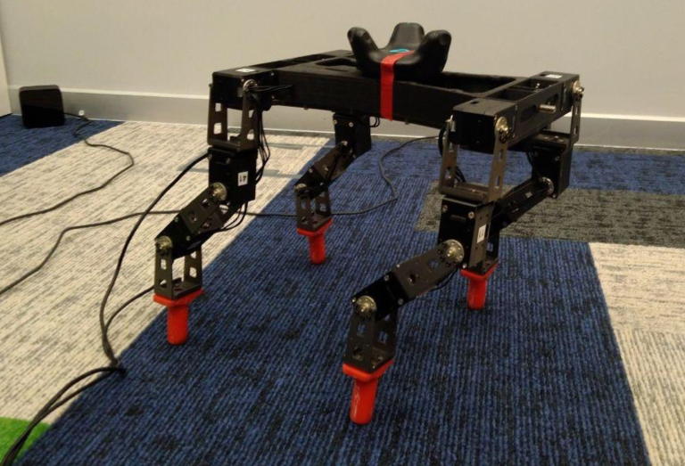
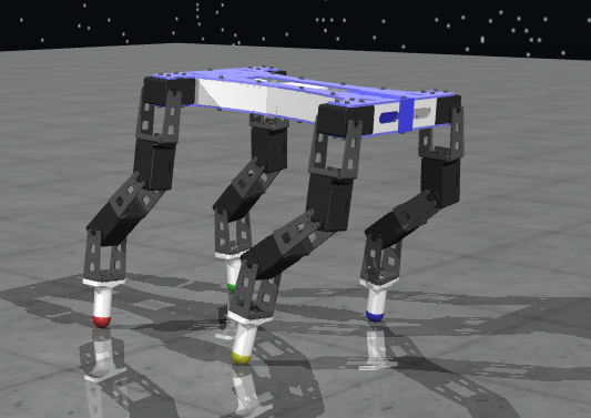
Figure 1: DKitty, quadruped robot with 12 degrees of freedom. (a) Real-world setup. (b) Visualization in MuJoCo engine.

Task set	Description
Direction	Destination point sampled randomly between ($0,2$) meters and ($0,-2$) meters with equal probability.
Friction	The friction coefficient is sampled from {$0.2,0.7,1.2$} with equal probability.
Angle	The floor incline angle is sampled from {$-15,-10,-5,0,5,10,15$} with equal probability.
Inverted actions	The middle joint in a randomly chosen leg is inverted (probability $=1/5$ for each leg) or no joints are inverted (probability $=1/5$).

Table 1: Benchmark task sets. The friction coefficient for all task sets except Friction is $\approx 1$. The incline angle for all task sets except Angle is zero. The destination point for all task sets except Direction is ($0,2$) meters.

5 Benchmarks in Simulation

We perform the meta-training entirely in simulation with domain randomizations, which are described in Appendix B. The subsequent tests have been performed both in simulation and the real environments. In the simulation tests, we compared the performance of two meta-learning algorithms MAML and PEARL (Table 2). PEARL needs at least three episodes (160 steps per episode) for each task to reach near 100% performance. On the other hand, MAML needs about 20 episodes or 3200 steps to tune to a concrete task, but shows inferior performance in spite of this handicap. This result is consistent with previous observations [18].

	PEARL			MAML
Task	return	success	end position	return	success	end position
direction	2110	100%	0.18	441	45%	0.82
friction	2058	100%	0.11	967	98%	0.23
angle	1912	100%	0.15	229	25%	0.71
inverted actions	1950	98%	0.13	749	88%	0.26

Table 2: Benchmarking meta-learning algorithms in simulation. The measurements for PEARL exclude the first three episodes (480 steps) during which the agent adapts to a given task. MAML acquires the context data for 20 episodes (3200 steps), after which a single inner-loop update step is made. The return column shows the average cumulative reward obtained by the agent in evaluation (see Appendix A for the reward details). Success is the average success rate. End position is the average distance between the robot and the target at the end of an episode.

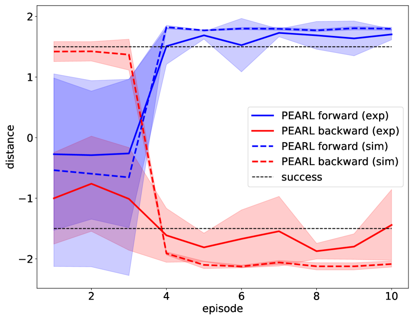
(a)

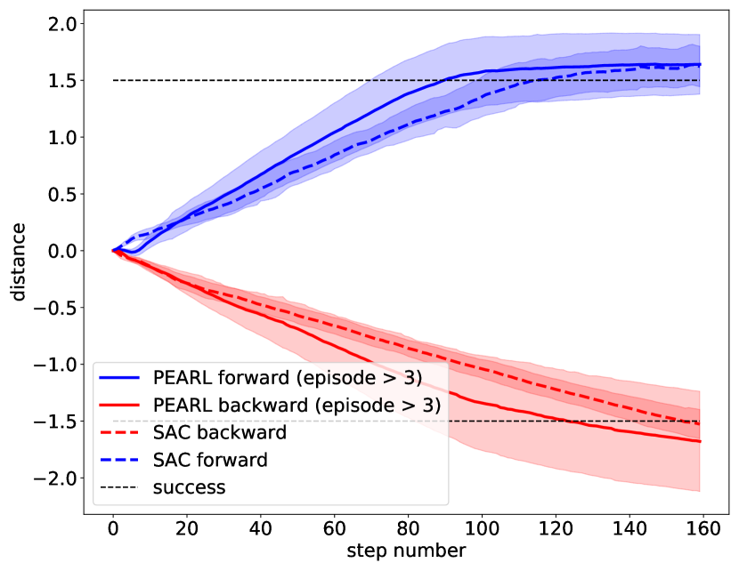
(b)

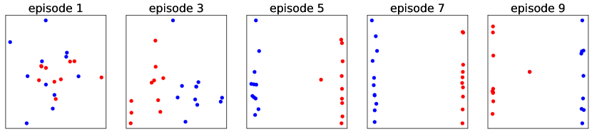
(c)

Figure 2: Direction tasks. (a) Distance to the destination point at the end of the episode as a function of the episode number. (b) Distance to the destination as a function of the step number for PEARL (averaged over episodes 4–10) compared to a SAC model trained on a single task, remarkably showing similar performance. (c) PCA of latent context vectors. Forward is blue, backward is red. After the first three episodes, the context vectors for the two tasks become distinguishable.

6 Benchmarks on Real Robot

Experimental results in a real-world setup are shown in Figs. 2, 3, 4, 5 for the four task sets studied; links to video footage can be found in Appendix D. All measurements represent 10 tests, each of which was run for 10 episodes for each task. We show the distance travelled by the robot as well as the first two dimensions of the vector obtained via principal component analysis (PCA) of the 5-dimensional PEARL latent context vector $z$. In the beginning of the test, the context buffer is small so the context vector, sampled from a Gaussian distribution (1), is almost random, and hence carries little information about the task. As the agent’s experience grows, the context vectors associated with the tasks become increasingly distinguishable. Complete distinguishability is typically reached by the fourth episode.

Figures 2 and 3 show the performance of PEARL in the Direction and Inverted actions task sets, respectively. The Direction results are shown both for simulation and real-world experiments, while the results for Inverted actions are for real-world only. As seen in parts (a) and (c) of both figures, the agent needs about 4 episodes to figure out the desired direction or the inverted limb. Starting from the 4th episode, it routinely succeeds in reaching its destination. Figure 2(b) shows the comparison of PEARL with a SAC model trained on a single task (either forward or backward locomotion). Remarkably, the performance of PEARL is the same (or better) than that of the single task agent.

For the Inverted actions task set, the performance of the robot with one of the fore legs inverted is poorer in comparison with that with an inverted hind leg, which, in turn, is similar to that of a robot without inversions.

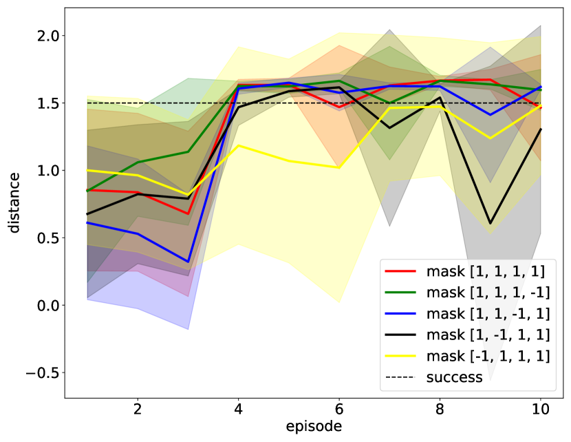
(a)

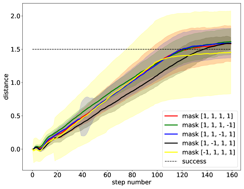
(b)

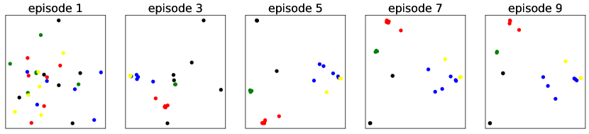
(c)

Figure 3: Inverted actions results: no inversion (blue), left hind leg (red), right hind leg (green), left fore leg (yellow), right fore leg (black). (a) Distance to the goal at the end of the episode (b) Distance to the goal as a function of the step number. (c) PCA of the latent context vectors.

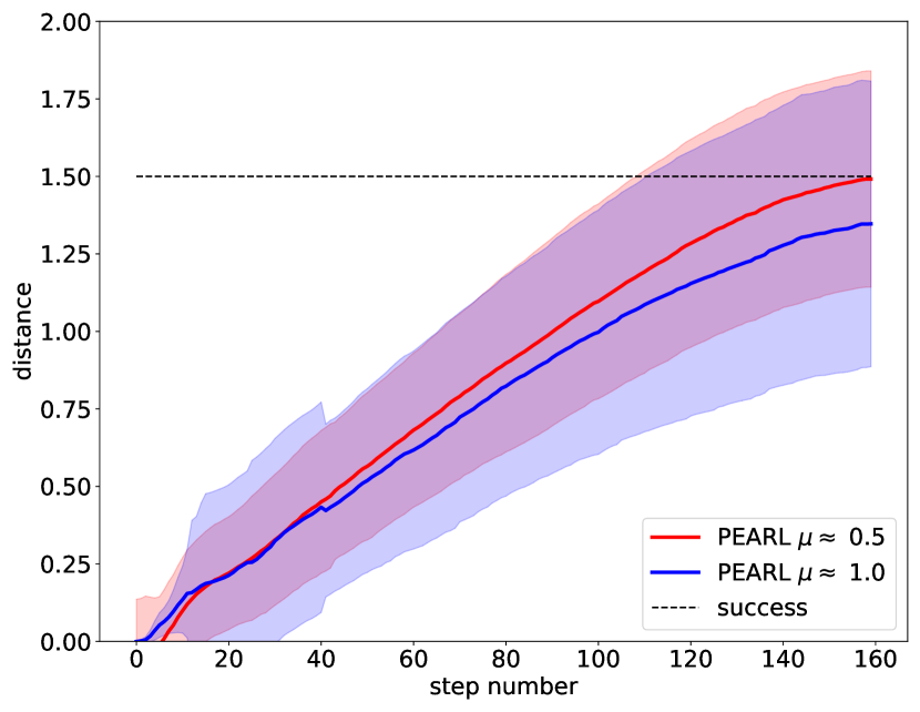
(a)

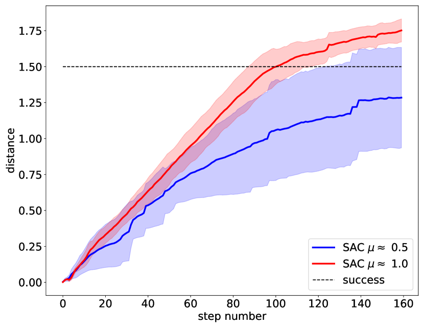
(b)

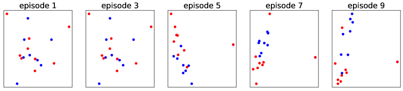
(c)

Figure 4: Friction tasks, with the friction coefficient $\mu\approx 0.5$ for a smooth table (red) and $\mu\approx 1.0$ for a carpet (blue). (a, b) Distance to the goal as a function of the step number for PEARL averaged across episodes 4–10 (a) and SAC (b). SAC’s performance is similar to that of PEARL. (c) PCA of latent context vectors.

Figures 4 and 5 show the agent performance on the Friction and Angle tasks. For the Friction set, the agent is tested in real-world on two surfaces: 1) smooth table with the friction coefficient $\mu\approx 0.5$ 2) carpet with the friction coefficient $\mu\approx 1.0$. We observe (Fig. 4(b)) that a single model SAC with the right domain randomization of the friction coefficient performs comparably with the meta-learned agent. In contrast, PEARL consistently outperforms single-task agents on the Angle tasks: both SAC and TQC fail to walk uphill (Fig. 5(c)) and TQC fails to walk downhill (Fig. 5(b)).

In addition to PEARL, we tested MAML on the Direction task set. This attempt however proved unsuccessful. The agent’s behavior under the pre-trained initial policy was significantly different in real world as compared to the simulation. As a result, the experience acquired under this policy was inadequate for the agent to fine-tune. We believe this observation to be a consequence of the fact that MAML, unlike PEARL, does not decouple task identification from policy optimization and hence has to use an on-policy inner loop algorithm. This algorithm does not benefit from domain randomization to the same extent as do state-of-the-art off-policy algorithms such as SAC.

7 Summary

We have shown real-world evaluation of meta-learning algorithms for quadruped robot locomotion control on a comprehensive set of benchmarks, such as walking on floors with different friction, walking on inclined planes and operating joints with inverted actions. The agents trained using PEARL on a particular multi-task set exhibit competitive performance in comparison with state-of-the-art off-policy RL algorithms trained on specific tasks within that set. This is a consequence of PEARL’s efficiency at identifying the task at hand. We confirmed this efficiency by principal components analysis of the latent context vectors, which shows the vectors associated with different tasks to be linearly separable in most cases.

Of particular interest are task sets with discrete parameter settings — such as Direction and Inverted actions. These task sets, while sharing the same dynamics, cannot be solved by simple domain randomization without informing the agent of the task explicitly or endowing it with a memory capacity [17]. These task sets naturally fall under the umbrella of meta-learning.

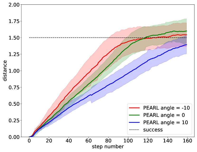
(a) PEARL; angle in {-10, 0, 10} degree

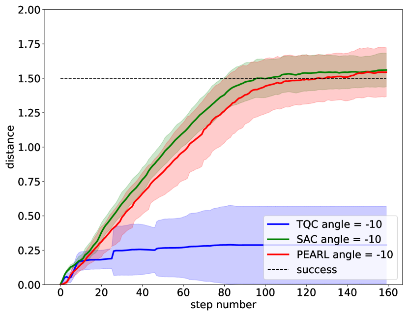
(b) PEARL, SAC, TQC; angle = -10 degree

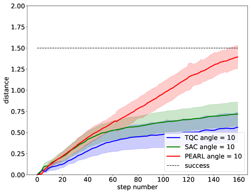
(c) PEARL, SAC, TQC; angle = 10 degree

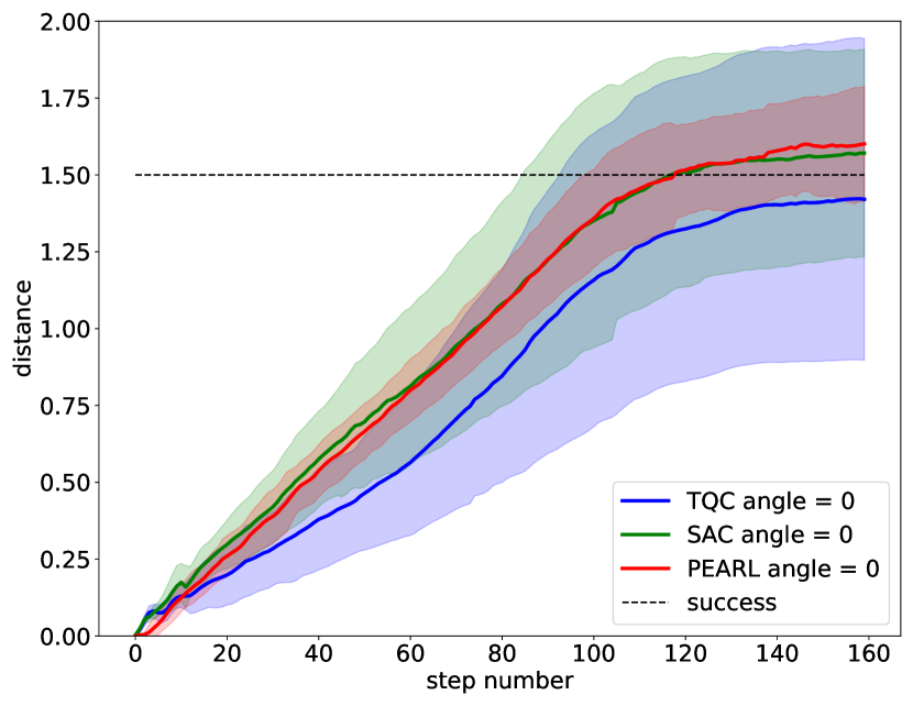
(d) PEARL, SAC, TQC; angle = 0 degree

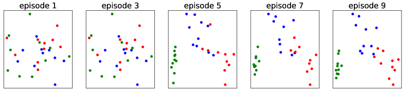
(e) PCA of context vectors: 0 (blue), 10 (red), -10 (green) degrees

Figure 5: Angle tasks. (a) Distance to the goal as a function of the step number. (b), (c), (d) Comparison of PEARL with SAC and TQC trained with angle domain randomizations for downhill (b), uphill (c) and even (d) floors. PEARL outperforms both single-task agents. (e) PCA of the latent context vector space. The agent can distinguish the three floor inclinations.

Acknowledgments

We thank Anton Zemerov for assembling DKitty, Nikolay Kuznetsov for printing robot parts and Vitaly Kurin for enlightening discussions.

Appendix A Robot Actions and Rewards

The reward function, taken from Ref. [5], is defined by $r=r_{\rm upright}-100\times r_{\rm falling}-4\times{\rm dist}+2\times r_{\rm heading}+5\times r_{\rm small\_bonus}+10\times r_{\rm big\_bonus}$, where the individual terms are:

• uprightness reward ($r_{\rm upright}$): $({\rm uprightness}-{\rm upright\_threshold})/(1-{\rm upright\_threshold})$, where ${\rm upright\_threshold}=0.9$;

• falling reward ($r_{\rm falling}$): $1$ if $\rm uprightness<\rm upright\_threshold$;

• reward for proximity to the target (${\rm dist}$): $|\rm robot\_position-\rm target\_position|$ in meters;

• heading reward ($r_{\rm heading}$): $(\rm heading-0.9)/0.1$, where ${\rm heading}$ is the cosine between the heading direction and torso orientation;

• small bonus: $(\rm dist<0.5)+(\rm heading>0.9)$;

• big bonus: $(\rm dist<0.5)\times(\rm heading>0.9)$.

Actions are the desired positions for the actuators.

Appendix B Domain randomizations

In order to bridge the reality gap for the trained models, we include the following randomizations in the MuJoCo simulator for DKitty:

• joint dynamics:

  • damping_range = $(0.1,0.2)$;

  • friction_loss_range = $(0.001,0.005)$.

• actuators strength:

  • kp_range = $(2.5,3.0)$.

• friction:

  • slide_range = $(0.8,1.2)$;

  • span_range = $(0.003,0.007)$;

  • roll_range = $(0.00005,0.00015)$.

• robot mass:

  • total_mass_range = $(1.6,2.0)$.

These randomizations are applied to all tasks and legs. Note that slide_range not applicable to meta-learning in the Friction task.

Appendix C Neural networks

In our work, we used code sources from original papers:

• PEARL: https://github.com/katerakelly/oyster;

• MAML: https://github.com/cbfinn/maml;

• TQC: https://github.com/SamsungLabs/tqc_pytorch.

The SAC implementation is based on Ref. [33], which is a modified version of the original SAC [32]. The critic and policy networks consist of three hidden layers with 256 neurons each and rectified linear (ReLU) activations.

The PEARL inference network $f_{\phi}$ is a multilayer perceptron consisting of three hidden layers with 200 neurons each and ReLU activations. It receives a transition $c_{n}=\{(s_{n},a_{n},r_{n},s^{\prime}_{n})\}$ as a concatenated vector and outputs the vectors of means $f^{\mu}_{\phi}(c_{n})$ and variances $f^{\sigma}_{\phi}(c_{n})$ of a 5-dimensional Gaussian distribution, which is used to sample a 5-dimensional latent context vector via Eq. (1). PEARL uses the original SAC inner loop with two critic networks, a single value network and a policy network (actor) [32]. Each network consists of three hidden layers with 300 neurons each and ReLU activations. The critics receive $(s_{n},a_{n},z)$ as a concatenated vector and output the action value. The value network receives $(s_{n},z)$ as an input and outputs the state value estimation. Finally, the policy network receives $(s_{n},z)$ and returns the parameters of a 12-dimensional Gaussian distribution with a diagonal covariance matrix, which corresponds to the 12-DoF robot actions.

Appendix D Videos

We recorded videos of the PEARL agent on the Direction task set as well as the SAC and PEARL agents on an Angle task with the floor at a 10-degree angle (uphill).

• Direction

  The PEARL agent is tested during the 10 adaptation episodes. At the beginning of each episode, the agent samples a random latent context vector $z$ and assumes the corresponding task throughout the episode. We found that almost the entire latent space embeds either of the two tasks, so sampling a random $z$ will likely compel the robot to determinedly navigate either forward or backward. Only a small section of that space contains samples that produce chaotic movements around the starting point.

  Video 1 shows that the agent may sample an incorrect task hypothesis made initially. After three or four adaptation episodes, however, it corrects the hypothesis and succeeds in solving the task in subsequent episodes.

• Angle

  The SAC agent fails to walk uphill and gets stuck about halfway to the destination (Video 2). The PEARL agent, on the other hand, successfully solves this task by adjusting its policy (Video 3, Fig. 5(c)). We can observe that the PEARL agent adapts to the specific angle by using hind legs as a lever and fore legs for support, placing them close to each other.

Appendix E Inverted Actions: Two Legs

We tested the PEARL agent on a previously unseen set of tasks in the Inverted Actions set: two middle joints inverted at the same time (Fig. 6). The real-world robot succeeded for a half of the tasks, the inverted joints being in the right fore leg + right hind leg, right and left hind legs, left fore leg + right hind leg. On the other tasks, the robot falls in the very beginning of the episode. In simulation, the agent successfully solves all the tasks except the one in which the right and left fore legs are inverted.

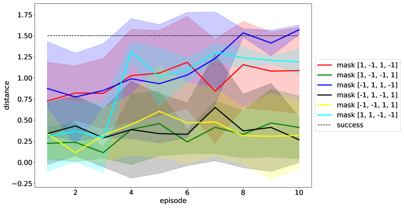
(a)

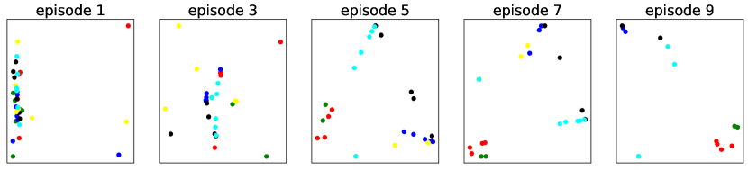
(b)

Figure 6: Results for the Inverted actions task set with simultaneously inverted two legs (tasks unseen during the training). (a) Distance to the goal at the end of the episode. The four values of the “mask” vectors in the legend correspond to, respectively, left fore, right fore, left hind and right hind legs; the value of $-1$ denotes inversion. (b) PCA analysis of the latent context vector. The vectors corresponding to the successfully completed tasks (red, blue and cyan) are well separated from each other.

References

- Sutton and Barto [2018] R. S. Sutton and A. G. Barto. Reinforcement learning: An introduction. MIT press, 2018.
- Li [2017] Y. Li. Deep Reinforcement Learning: An Overview. arXiv e-prints, art. arXiv:1701.07274, Jan. 2017.
- Silver et al. [2021] D. Silver, S. Singh, D. Precup, and R. S. Sutton. Reward is enough. Artificial Intelligence, 299, 2021. doi:10.1016/j.artint.2021.103535.
- Haarnoja et al. [2018] T. Haarnoja, S. Ha, A. Zhou, J. Tan, G. Tucker, and S. Levine. Learning to Walk via Deep Reinforcement Learning. arXiv e-prints, art. arXiv:1812.11103, Dec. 2018.
- Ahn et al. [2019] M. Ahn, H. Zhu, K. Hartikainen, H. Ponte, A. Gupta, S. Levine, and V. Kumar. ROBEL: Robotics Benchmarks for Learning with Low-Cost Robots. arXiv e-prints, art. arXiv:1909.11639, Sept. 2019.
- Lee et al. [2020] J. Lee, J. Hwangbo, L. Wellhausen, V. Koltun, and M. Hutter. Learning Quadrupedal Locomotion over Challenging Terrain. arXiv e-prints, art. arXiv:2010.11251, Oct. 2020.
- Peng et al. [2017] X. B. Peng, M. Andrychowicz, W. Zaremba, and P. Abbeel. Sim-to-Real Transfer of Robotic Control with Dynamics Randomization. arXiv e-prints, art. arXiv:1710.06537, Oct. 2017.
- OpenAI et al. [2019] OpenAI, I. Akkaya, M. Andrychowicz, M. Chociej, M. Litwin, B. McGrew, A. Petron, A. Paino, M. Plappert, G. Powell, R. Ribas, J. Schneider, N. Tezak, J. Tworek, P. Welinder, L. Weng, Q. Yuan, W. Zaremba, and L. Zhang. Solving Rubik’s Cube with a Robot Hand. arXiv e-prints, art. arXiv:1910.07113, Oct. 2019.
- Zeng et al. [2019] A. Zeng, S. Song, J. Lee, A. Rodriguez, and T. Funkhouser. TossingBot: Learning to Throw Arbitrary Objects with Residual Physics. arXiv e-prints, art. arXiv:1903.11239, Mar. 2019.
- Zhu et al. [2018] H. Zhu, A. Gupta, A. Rajeswaran, S. Levine, and V. Kumar. Dexterous Manipulation with Deep Reinforcement Learning: Efficient, General, and Low-Cost. arXiv e-prints, art. arXiv:1810.06045, Oct. 2018.
- Nagabandi et al. [2019] A. Nagabandi, K. Konoglie, S. Levine, and V. Kumar. Deep Dynamics Models for Learning Dexterous Manipulation. arXiv e-prints, art. arXiv:1909.11652, Sept. 2019.
- Jang et al. [2018] E. Jang, C. Devin, V. Vanhoucke, and S. Levine. Grasp2Vec: Learning Object Representations from Self-Supervised Grasping. arXiv e-prints, art. arXiv:1811.06964, Nov. 2018.
- Kalashnikov et al. [2018] D. Kalashnikov, A. Irpan, P. Pastor, J. Ibarz, A. Herzog, E. Jang, D. Quillen, E. Holly, M. Kalakrishnan, V. Vanhoucke, and S. Levine. QT-Opt: Scalable Deep Reinforcement Learning for Vision-Based Robotic Manipulation. arXiv e-prints, art. arXiv:1806.10293, June 2018.
- Zhao et al. [2020] W. Zhao, J. Peña Queralta, and T. Westerlund. Sim-to-Real Transfer in Deep Reinforcement Learning for Robotics: a Survey. arXiv e-prints, art. arXiv:2009.13303, Sept. 2020.
- Tobin et al. [2017] J. Tobin, R. Fong, A. Ray, J. Schneider, W. Zaremba, and P. Abbeel. Domain Randomization for Transferring Deep Neural Networks from Simulation to the Real World. arXiv e-prints, art. arXiv:1703.06907, Mar. 2017.
- Mehta et al. [2019] B. Mehta, M. Diaz, F. Golemo, C. J. Pal, and L. Paull. Active Domain Randomization. arXiv e-prints, art. arXiv:1904.04762, Apr. 2019.
- Yu et al. [2019] T. Yu, D. Quillen, Z. He, R. Julian, K. Hausman, C. Finn, and S. Levine. Meta-World: A Benchmark and Evaluation for Multi-Task and Meta Reinforcement Learning. arXiv e-prints, art. arXiv:1910.10897, Oct. 2019.
- Rakelly et al. [2019] K. Rakelly, A. Zhou, D. Quillen, C. Finn, and S. Levine. Efficient Off-Policy Meta-Reinforcement Learning via Probabilistic Context Variables. arXiv e-prints, art. arXiv:1903.08254, Mar. 2019.
- Finn et al. [2017] C. Finn, P. Abbeel, and S. Levine. Model-Agnostic Meta-Learning for Fast Adaptation of Deep Networks. arXiv e-prints, art. arXiv:1703.03400, Mar. 2017.
- Zhao et al. [2020] T. Z. Zhao, A. Nagabandi, K. Rakelly, C. Finn, and S. Levine. MELD: Meta-Reinforcement Learning from Images via Latent State Models. arXiv e-prints, art. arXiv:2010.13957, Oct. 2020.
- Duan et al. [2016] Y. Duan, J. Schulman, X. Chen, P. L. Bartlett, I. Sutskever, and P. Abbeel. RL2: Fast Reinforcement Learning via Slow Reinforcement Learning. arXiv e-prints, art. arXiv:1611.02779, Nov. 2016.
- OpenAI et al. [2018] OpenAI, M. Andrychowicz, B. Baker, M. Chociej, R. Jozefowicz, B. McGrew, J. Pachocki, A. Petron, M. Plappert, G. Powell, A. Ray, J. Schneider, S. Sidor, J. Tobin, P. Welinder, L. Weng, and W. Zaremba. Learning Dexterous In-Hand Manipulation. arXiv e-prints, art. arXiv:1808.00177, Aug. 2018.
- Sorokin et al. [2020] D. Sorokin, A. Ulanov, E. Sazhina, and A. Lvovsky. Interferobot: aligning an optical interferometer by a reinforcement learning agent. arXiv e-prints, art. arXiv:2006.02252, June 2020.
- Bousmalis et al. [2017] K. Bousmalis, A. Irpan, P. Wohlhart, Y. Bai, M. Kelcey, M. Kalakrishnan, L. Downs, J. Ibarz, P. Pastor, K. Konolige, S. Levine, and V. Vanhoucke. Using Simulation and Domain Adaptation to Improve Efficiency of Deep Robotic Grasping. arXiv e-prints, art. arXiv:1709.07857, Sept. 2017.
- Du et al. [2021] Y. Du, O. Watkins, T. Darrell, P. Abbeel, and D. Pathak. Auto-Tuned Sim-to-Real Transfer. arXiv e-prints, art. arXiv:2104.07662, Apr. 2021.
- Zintgraf et al. [2019] L. Zintgraf, K. Shiarlis, M. Igl, S. Schulze, Y. Gal, K. Hofmann, and S. Whiteson. VariBAD: A Very Good Method for Bayes-Adaptive Deep RL via Meta-Learning. arXiv e-prints, art. arXiv:1910.08348, Oct. 2019.
- Mitchell et al. [2020] E. Mitchell, R. Rafailov, X. B. Peng, S. Levine, and C. Finn. Offline Meta-Reinforcement Learning with Advantage Weighting. arXiv e-prints, art. arXiv:2008.06043, Aug. 2020.
- Nagabandi et al. [2018] A. Nagabandi, I. Clavera, S. Liu, R. S. Fearing, P. Abbeel, S. Levine, and C. Finn. Learning to Adapt in Dynamic, Real-World Environments Through Meta-Reinforcement Learning. arXiv e-prints, art. arXiv:1803.11347, Mar. 2018.
- Kingma and Welling [2013] D. P. Kingma and M. Welling. Auto-Encoding Variational Bayes. arXiv e-prints, art. arXiv:1312.6114, Dec. 2013.
- Jimenez Rezende et al. [2014] D. Jimenez Rezende, S. Mohamed, and D. Wierstra. Stochastic Backpropagation and Approximate Inference in Deep Generative Models. arXiv e-prints, art. arXiv:1401.4082, Jan. 2014.
- Alemi et al. [2016] A. A. Alemi, I. Fischer, J. V. Dillon, and K. Murphy. Deep Variational Information Bottleneck. arXiv e-prints, art. arXiv:1612.00410, Dec. 2016.
- Haarnoja et al. [2018a] T. Haarnoja, A. Zhou, P. Abbeel, and S. Levine. Soft Actor-Critic: Off-Policy Maximum Entropy Deep Reinforcement Learning with a Stochastic Actor. arXiv e-prints, art. arXiv:1801.01290, Jan. 2018a.
- Haarnoja et al. [2018b] T. Haarnoja, A. Zhou, K. Hartikainen, G. Tucker, S. Ha, J. Tan, V. Kumar, H. Zhu, A. Gupta, P. Abbeel, and S. Levine. Soft Actor-Critic Algorithms and Applications. arXiv e-prints, art. arXiv:1812.05905, Dec. 2018b.
- Schulman et al. [2015] J. Schulman, P. Moritz, S. Levine, M. Jordan, and P. Abbeel. High-Dimensional Continuous Control Using Generalized Advantage Estimation. arXiv e-prints, art. arXiv:1506.02438, June 2015.
- Kuznetsov et al. [2020] A. Kuznetsov, P. Shvechikov, A. Grishin, and D. Vetrov. Controlling Overestimation Bias with Truncated Mixture of Continuous Distributional Quantile Critics. arXiv e-prints, art. arXiv:2005.04269, May 2020.
- Fujimoto et al. [2018] S. Fujimoto, H. van Hoof, and D. Meger. Addressing Function Approximation Error in Actor-Critic Methods. arXiv e-prints, art. arXiv:1802.09477, Feb. 2018.
- Nachum et al. [2019] O. Nachum, M. Ahn, H. Ponte, S. Gu, and V. Kumar. Multi-Agent Manipulation via Locomotion using Hierarchical Sim2Real. arXiv e-prints, art. arXiv:1908.05224, Aug. 2019.
- Sharma et al. [2020] A. Sharma, M. Ahn, S. Levine, V. Kumar, K. Hausman, and S. Gu. Emergent Real-World Robotic Skills via Unsupervised Off-Policy Reinforcement Learning. arXiv e-prints, art. arXiv:2004.12974, Apr. 2020.