Wilson loops in the abelian lattice Higgs model

Abstract.

We consider the lattice Higgs model on $\mathbb{Z}^{4}$ in the fixed length limit, with structure group given by $\mathbb{Z}_{n}$ for $n\geqslant 2$. We compute the expected value of the Wilson loop observable to leading order when the inverse temperature and hopping parameter are both sufficiently large compared to the length of the loop. The leading order term is expressed in terms of a quantity arising from the related but much simpler $\mathbb{Z}_{n}$ model, which reduces to the usual Ising model when $n=2$. As part of the proof, we construct a coupling between the lattice Higgs model and the $\mathbb{Z}_{n}$ model.

1. Introduction

1.1. Background

Lattice gauge theories were introduced by Wilson [32] (see also Wegner [31]) as lattice approximations of quantum field theories known as (Yang–Mills) gauge theories. Gauge theories appear for instance in the Standard Model, where they describe fundamental particle interactions. One advantage of the lattice models is that they are immediately mathematically well-defined, whereas it remains a substantial problem to give rigorous constructions of relevant continuum theories [23]. In fact, one possible approach to the latter problem is to try passing to a scaling limit with a lattice theory.

A discrete gauge field configuration assigns to each lattice edge an element of a given group $G$, known as the structure (or gauge-) group, and can be thought of as a discrete approximation of a connection one-form on a principal $G$-bundle on an underlying smooth manifold. The simplest lattice gauge theory is a pure gauge theory, realized as a probability measure on gauge field configurations. The choice of structure group is part of the model and is fixed at the outset. The action that Wilson introduced in [32] (and which determines the probability measure) involves a discrete analog of curvature obtained by considering microscopic holonomies around lattice plaquettes. The definition is set up in such a way that the resulting discrete action is exactly invariant with respect to gauge transformations of the discrete configuration space, while still approximating the continuum Yang–Mills action in an appropriate lattice size scaling limit.

In the physics community, lattice gauge theories have been studied as statistical mechanics models in their own right, and have also been used as a basis for numerical simulations of the corresponding continuum models. Recently there has been a renewed interest in the rigorous analysis of four-dimensional gauge theories in the mathematical community using probabilistic techniques (see, e.g., [9, 6, 16, 8, 14, 19]). For example, in the papers [9, 6, 16], the leading order terms for the expectation of Wilson loop observables (see below) were computed for pure gauge theories with Wilson action and finite structure groups in the limit when the size of the loop and inverse temperature tend to infinity simultaneously in such a way that the Wilson loop expectation is non-trivial. (Structure groups that are of primary relevance to unresolved problems in physics, such as $SU(N)$, appear to be out of reach at the moment.) This type of result was first obtained by Chatterjee in [9] and is different from the more classical results on area versus perimeter law (see, e.g., [26, 17, 5, 32, 27, 18]), which concern the decay rate of the Wilson loop expectation as the size of the loop tends to infinity while the inverse temperature is kept fixed. Part of the motivation for the results in this paper instead stems from the question of how to renormalize in order to be able to take a scaling limit. We will comment further on this below.

Pure gauge theories model only the gauge field itself, and in order to advance towards physically relevant theories, it is necessary to consider models that include matter fields interacting with the gauge field, see, e.g., [17, 27]. In this paper, we consider lattice gauge theories with Wilson’s action for the gauge field, coupled to a scalar Bosonic field with a quartic Higgs potential. The resulting theory is called the lattice Higgs model. We analyze this model in a particular limiting “fixed length” regime where the relative weight of the potential is infinite, forcing the Higgs field to have unit length. We only consider finite abelian structure groups.

We will discuss the relation to previous work in more detail below, but let us now mention that the models we consider here have received significant attention in the physics literature: see for instance the works [1, 2, 3], where calculations to obtain critical parameters of these models were first performed, and [24, 25], in which phase diagrams were sketched. For further background, as well as more references, we refer the reader to [17] and [30].

Just as in [9, 16, 6] our main goal is to analyze the asymptotic behavior of Wilson loop expectations, that is, expected values of “holonomy variables”, computed along large loops when the inverse temperature is also large compared to the perimeter of the loop. Wilson introduced such observables as a means to detect whether quark confinement occurs, see [32], and they have since been a primary focus in the analysis of lattice gauge theories. Here we compute the leading order term of the Wilson loop expectation (in the sense of [9, 16, 6]) in the lattice Higgs model in the fixed length regime. We show that the leading order term can be expressed in terms of the expectation of a certain observable in a simpler $\mathbb{Z}_{n}$ model of interacting spins on vertices. (In the case $n=2$ this is the Ising model.) Our theorems are of a similar type as the main results of [9, 16, 6], but require substantial additional work due to the presence of an interacting field. Along the way, we develop tools that we believe may be useful to analyze other gauge theories coupled with matter fields, as well as other observables in the lattice Higgs model. In particular, we construct a coupling, in the sense of probability measures, of the lattice Higgs model and the $\mathbb{Z}_{n}$ model, thereby making precise certain ideas appearing in the physics literature, see, e.g., [17, Section C]. We note however that we do not consider the question of lattice fields acquiring “mass” due to the presence of a Higgs field and the breaking of an exact gauge symmetry (see Section 2.2), cf., e.g., Section 4 of [27].

1.2. Preliminary notation

For $m\geqslant 2$, the graph $\mathbb{Z}^{m}$ has a vertex at each point $x\in\mathbb{Z}^{m}$ with integer coordinates and a non-oriented edge between nearest neighbors. We will work with oriented edges throughout this paper, and for this reason we associate to each non-oriented edge $\bar{e}$ in $\mathbb{Z}^{m}$ two oriented edges $e_{1}$ and $e_{2}=-e_{1}$ with the same endpoints as $\bar{e}$ and opposite orientations.

Let $d\mathbf{e}_{1}\coloneqq(1,0,0,\ldots,0)$, $d\mathbf{e}_{2}\coloneqq(0,1,0,\ldots,0)$, …, $d\mathbf{e}_{m}\coloneqq(0,\ldots,0,1)$ be oriented edges corresponding to the unit vectors in $\mathbb{Z}^{m}$. We say that an oriented edge $e$ is positively oriented if it is equal to a translation of one of these unit vectors, i.e., if there is a $v\in\mathbb{Z}^{m}$ and a $j\in\{1,2,\ldots,m\}$ such that $e=v+d{\mathbf{e}}_{j}$. When two vertices $x$ and $y$ in $\mathbb{Z}^{m}$ are adjacent, we sometimes write $(x,y)$ to denote the oriented edge with endpoints at $x$ and $y$ which is oriented from $x$ to $y$. If $v\in\mathbb{Z}^{m}$ and $j_{1}<j_{2}$, then $p=(v+d\mathbf{e}_{j_{1}})\land(v+d\mathbf{e}_{j_{2}})$ is a positively oriented 2-cell, also known as a positively oriented plaquette. We let $B_{N}$ denote the set $[-N,N]^{m}$ of $\mathbb{Z}^{m}$, and we let $V_{N}$, $E_{N}$, and $P_{N}$ denote the sets of oriented vertices, edges, and plaquettes, respectively, whose end-points are all in $B_{N}$.

Whenever we talk about lattice gauge theory we do so with respect to some (abelian) group $(G,+)$, referred to as the structure group. We also fix a unitary and faithful representation $\rho$ of $(G,+)$. In this paper, we will always assume that $G=\mathbb{Z}_{n}$ for some $n\geqslant 2$ with the group operation $+$ given by standard addition modulo $n$. Also, we will assume that $\rho$ is a one-dimensional representation of $G$. We note that a natural such representation is $j\mapsto e^{j\cdot 2\pi i/n}$.

Now assume that a structure group $(G,+)$, a one-dimensional unitary representation $\rho$ of $(G,+)$, and an integer $N\geqslant 1$ are given. We let $\Sigma_{E_{N}}$ denote the set of all $G$-valued 1-forms $\sigma$ on $E_{N}$, i.e., the set of all $G$-valued functions $\sigma\colon e\mapsto\sigma_{e}$ on $E_{N}$ such that $\sigma_{e}=-\sigma_{-e}$ for all $e\in E_{N}$. We let $\hat{\Phi}_{V_{N}}$ denote the set of all $\mathbb{C}$-valued functions $\phi\colon x\mapsto\phi_{x}$ on $V_{N}$ which satisfy $\phi_{x}/|\phi_{x}|\in\rho(G)$ for $x\in V_{N}$ and $\phi_{x}=0$ for $x\notin V_{N}$. Similarly, we let $\Phi_{V_{N}}$ denote the set of all $\phi\in\hat{\Phi}_{V_{N}}$ such that $\phi_{x}\in\rho(G)$ for each $x\in V_{N}$. When $\sigma\in\Sigma_{E_{N}}$ and $p\in P_{N}$, we let $\partial p$ denote the four edges in the oriented boundary of $p$ (see Section 2.1.4), and define

$$(d\sigma)_{p}\coloneqq\sum_{e\in\partial p}\sigma_{e}.$$

Elements $\sigma\in\Sigma_{E_{N}}$ will be referred to as gauge field configurations, and elements $\phi\in\hat{\Phi}_{V_{N}}$ will be referred to as Higgs field configurations.

1.3. Lattice Higgs model and Wilson loops

The Wilson action functional for pure gauge theory is defined by (see, e.g., [32])

$$S^{W}(\sigma)\coloneqq-\sum_{p\in P_{N}}\rho((d\sigma)_{p}),\quad\sigma\in\Sigma_{E_{N}}.$$

For $\sigma\in\Sigma_{E_{N}}$ and $e=(x,y)\in E_{N}$, we define a discrete covariant derivative of $\phi\in\hat{\Phi}_{V_{N}}$ along $e$ by

$$D_{e}\phi\coloneqq\rho(\sigma_{-e})\phi_{y}-\phi_{x}.$$

Then, for $\sigma\in\Sigma_{E_{N}}$ and $\phi\in\hat{\Phi}_{V_{N}}$, we define the corresponding kinetic action by the Dirichlet energy

$$S^{D}(\sigma,\phi)\coloneqq\frac{1}{2}\sum_{e\in E_{N}}|D_{e}\phi|^{2}=\frac{1}{2}\sum_{e=(x,y)\in E_{N}}\overline{(\rho(\sigma_{-e})\phi_{y}-\phi_{x})}(\rho(\sigma_{-e})\phi_{y}-\phi_{x})$$

$$\qquad=\frac{1}{2}\sum_{e=(x,y)\in E_{N}}\Bigl{(}|\phi_{x}|^{2}+|\phi_{y}|^{2}-\overline{\phi_{y}}\overline{\rho(\sigma_{-e})}\phi_{x}-\overline{\phi_{x}}\rho(\sigma_{-e})\phi_{y}\Bigr{)}$$

$$\qquad=\sum_{x\in V_{N}}\bigl{|}\{e\in E_{N}\colon x\in\partial e\}\bigr{|}\,|\phi_{x}|^{2}+S^{I}(\sigma,\phi),$$

where the interaction term $S^{I}$ is given by

$$S^{I}(\sigma,\phi)\coloneqq-\sum_{e=(x,y)\in E_{N}}\overline{\phi_{y}}\rho(\sigma_{e})\phi_{x}.$$

We finally consider a quartic “sombrero” potential

$$V(\phi)\coloneqq\sum_{x\in V_{N}}\bigl{(}|\phi_{x}|^{2}-1\bigr{)}^{2},\quad\phi\in\hat{\Phi}_{V_{N}}.$$

Given $\beta,\kappa,\zeta\geqslant 0$, the action $S_{\beta,\kappa,\zeta}$ for lattice gauge theory with Wilson action coupled to a Higgs field on $B_{N}$ is, for $\sigma\in\Sigma_{E_{N}}$ and $\phi\in\hat{\Phi}_{V_{N}}$, defined by

$$\begin{split}&S_{\beta,\kappa,\zeta}(\sigma,\phi)\coloneqq\beta S^{W}(\sigma)+S^{D}(\sigma,\phi)+(\kappa-1)S^{I}(\sigma,\phi)+\zeta V(\phi)\\ &\qquad=-\beta\sum_{p\in P_{N}}\rho((d\sigma)_{p})-\kappa\sum_{e=(x,y)\in E_{N}}\overline{\phi_{y}}\rho(\sigma_{e}){\phi_{x}}\\ &\qquad\qquad+\zeta\sum_{x\in V_{N}}\bigl{(}|\phi_{x}|^{2}-1\bigr{)}^{2}+\sum_{x\in V_{N}}\bigl{|}\{e\in E_{N}\colon x\in\partial e\}\bigr{|}\,|\phi_{x}|^{2}.\end{split}$$ (1.1)

The corresponding Gibbs measure can be written

$$d\mu_{N,\beta,\kappa,\zeta}(\sigma,\phi)=Z^{-1}_{N,\beta,\kappa,\zeta}e^{-S_{\beta,\kappa,\zeta}(\sigma,\phi)}\prod_{e\in E_{N}^{+}}d\mu_{G}(\sigma_{e})\prod_{x\in V_{N}}d\mu_{\rho(G)}(\phi_{x}/|\phi_{x}|)d\mu_{\mathbb{R}_{+}}(|\phi_{x}|),$$

where $E_{N}^{+}$ denotes the set of positively oriented edges in $E_{N}$, $d\mu_{G}$ is the uniform measure on $G$, $d\mu_{\rho(G)}$ is the uniform measure on $\rho(G)$, and $\mu_{\mathbb{R}_{+}}$ is the Lebesgue measure on $\mathbb{R}_{+}$. We refer to this lattice gauge theory as the lattice Higgs model. Since $\sigma\in\Sigma_{E_{N}}$, we have $\rho(\sigma_{-e})=\overline{\rho(\sigma_{e})}$, and hence $S_{\beta,\kappa,\zeta}(\sigma,\phi)$ is real for all $\sigma\in\Sigma_{E_{N}}$ and $\phi\in\hat{\Phi}_{V_{N}}$. The quantity $\beta$ is known as the gauge coupling constant (or inverse temperature), $\kappa$ is known as the hopping parameter, and $\zeta$ is known as the quartic Higgs self coupling. We will work with the model obtained from this action in the fixed length limit $\zeta\to\infty$, in which the Higgs field concentrates on the unit circle, i.e., $|\phi_{x}|=1$ for all $x\in V_{N}$. (This is sometimes called the London limit in the physics literature.) We do not discuss the limit of the Gibbs measure corresponding to $S_{\beta,\kappa,\zeta}$ as $\zeta\to\infty$, but simply from the outset adopt the action resulting from only considering $\phi\in\Phi_{V_{N}}$, so that $|\phi_{x}|=1$ for all $x\in V_{N}$:

$$\begin{split}&S_{\beta,\kappa,\infty}(\sigma,\phi)\coloneqq\beta S^{W}(\sigma)+\kappa S^{I}(\sigma,\phi)\\ &\qquad=-\beta\sum_{p\in P_{N}}\rho((d\sigma)_{p})-\kappa\sum_{e=(x,y)\in E_{N}}\overline{\phi_{y}}\rho(\sigma_{e}){\phi_{x}},\quad\sigma\in\Sigma_{E_{N}},\,\phi\in\Phi_{V_{N}}.\end{split}$$ (1.2)

We then consider a corresponding probability measure $\mu_{N,\beta,\kappa,\infty}$ on $\Sigma_{E_{N}}\times\Phi_{V_{N}}$ given by

$$\mu_{N,\beta,\kappa,\infty}(\sigma,\phi)\coloneqq Z_{N,\beta,\kappa,\infty}^{-1}e^{-S_{\beta,\kappa,\infty}(\sigma,\phi)},\quad\sigma\in\Sigma_{E_{N}},\,\phi\in\Phi_{V_{N}},$$ (1.3)

where $Z_{N,\beta,\kappa,\infty}$ is a normalizing constant. This is the fixed length lattice Higgs model. We let $\mathbb{E}_{N,\beta,\kappa,\infty}$ denote the corresponding expectation. In the physics literature, this model has been studied in, e.g., [12, 24, 22, 10] (see also the review [17]). In [11, 25], phase diagrams for the theory described by (1.1) are sketched. These diagrams suggest (see also, e.g., [30]) that for large $\zeta$, the model described by (1.1) behaves very similarly to the fixed length model considered here.

Observables attached to simple oriented loops in the underlying lattice are among the main objects of interest in lattice gauge theories. If $\gamma\subseteq E_{N}$ is such that

1. if $e\in\gamma$ then $-e\notin\gamma$, and

2. the edges in $\gamma$ can be ordered so that they form an oriented loop,

then we say that $\gamma$ is a simple loop in $E_{N}$. If $\gamma$ is a simple loop in $E_{N}$ for some $N\geqslant 1$, then we say that $\gamma$ is a simple loop in $\mathbb{Z}^{m}$. Given a gauge field configuration $\sigma\in\Sigma_{E_{N}}$, the Wilson loop observable $W_{\gamma}$ is defined by considering the discrete holonomy along $\gamma$:

$$W_{\gamma}\coloneqq\rho\Bigl{(}\sum_{e\in\gamma}\sigma_{e}\Bigr{)}.$$ (1.4)

Wilson argued that the decay rate of the expected value of $W_{\gamma}$ carries information about whether quark confinement occurs in the model, see [32].

Figure 1 shows the results of two simulations of the fixed length lattice Higgs model on $\mathbb{Z}^{2}.$

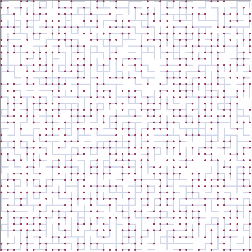
a $\kappa=0$

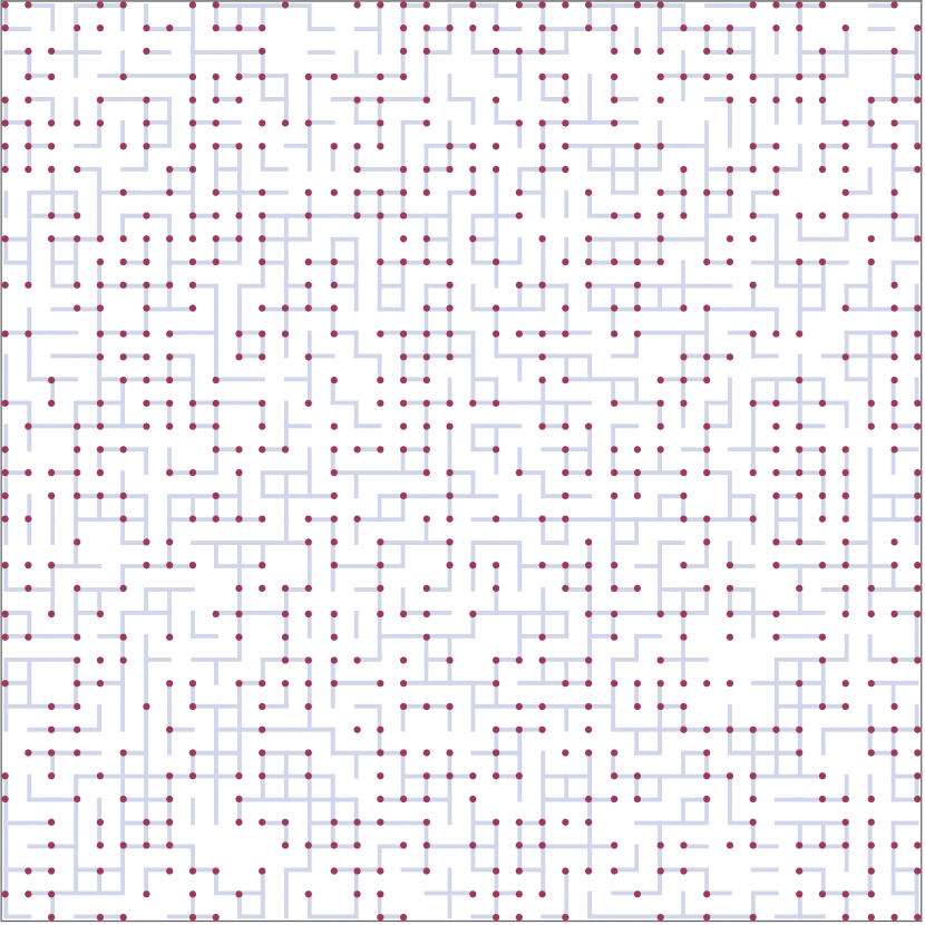
b $\kappa=0.3$

c $\kappa=0.5$

d $\kappa=0$

e $\kappa=0.3$

f $\kappa=0.5$

Figure 1. In 1a, 1b, and 1c, we draw configurations $(\sigma,\phi)$ obtained by simulation of the fixed length lattice Higgs model on a subset of $\mathbb{Z}^{2}$, using $G=\mathbb{Z}_{2}$, $\beta=2.2$, and free boundary conditions. In 1a, 1b, and 1c, the colored edges correspond to edges $e$ where the gauge field $\sigma_{e}\neq 0$, and the red dots to vertices $x$ where the Higgs field $\phi_{x}\neq 1$. In 1d, 1e, and 1f, we draw the same configurations as in 1a, 1b, and 1c, but here the colored edges instead correspond to edges $e=(x,y)$ with $\overline{\phi_{y}}\rho(\sigma_{e})\phi_{x}\neq 1$, and the colored squares to plaquettes $p$ with $(d\sigma)_{p}\neq 0$.

1.4. Main results

We define the measure $\mu_{N,\infty,\kappa}$ on $\Sigma_{E_{N}}^{0}\coloneqq\{\sigma\in\Sigma_{E_{N}}\colon d\sigma=0\}$ by

$$\mu_{N,\infty,\kappa}(\sigma)\coloneqq Z_{N,\infty,\kappa}^{-1}e^{\kappa\sum_{e\in E_{N}}\rho(\sigma_{e})},\quad\sigma\in\Sigma_{E_{N}}^{0},$$ (1.5)

where $Z_{N,\infty,\kappa}$ is a normalizing constant, and let $\mathbb{E}_{N,\infty,\kappa}$ denote the corresponding expectation. We note that if $G=\mathbb{Z}_{2}$, then $\mu_{N,\infty,\kappa}$ represents the gradient field of the standard Ising model in the following sense. If $\eta\in\mathbb{Z}_{2}^{V_{N}}$ is a spin configuration on $V_{N}$, chosen according to the Ising model with coupling parameter $\kappa$, and we for $e=(x,y)\in E_{N}$ let $\sigma_{e}\coloneqq\eta_{y}-\eta_{x}$, then $(\sigma_{e})_{e\in E_{N}}\sim\mu_{N,\infty,\kappa}$. In the same way, if $G=\mathbb{Z}_{n}$ for some $n\geqslant 3$, then $\mu_{N,\infty,\kappa}$ describes the distribution of the gradient field of the $\mathbb{Z}_{n}$ model (also known as the clock model).

For $\beta,\kappa\geqslant 0$, we let $\langle W_{\gamma}\rangle_{\beta,\kappa}$ and $\langle W_{\gamma}\rangle_{\infty,\kappa}$ denote the infinite volume limits

$$\langle W_{\gamma}\rangle_{\beta,\kappa}\coloneqq\lim_{N\to\infty}\mathbb{E}_{N,\beta,\kappa,\infty}[W_{\gamma}]\quad\text{and}\quad\langle W_{\gamma}\rangle_{\infty,\kappa}\coloneqq\lim_{N\to\infty}\mathbb{E}_{N,\infty,\kappa}[W_{\gamma}],$$ (1.6)

which are guaranteed to exist by the Ginibre inequalities (see Section 2.3).

Finally, given a simple loop $\gamma$, we let $\gamma_{c}$ denote the set of corner edges in $\gamma$, that is, the set of edges $e\in\gamma$ which share a plaquette with at least one other edge in $\pm\gamma$.

We are now ready to state our first main result.

Theorem 1.1.

Consider the fixed length lattice Higgs model on $\mathbb{Z}^{4}$, with structure group $G=\mathbb{Z}_{2}$, and representation $\rho\colon G\to\mathbb{C}$ given by $\rho(0)=1$ and $\rho(1)=-1$. Suppose that $\beta_{0},\kappa_{0}\geqslant 0$ satisfy

1. $e^{-4\beta_{0}}+4e^{-4\kappa_{0}}<1$,

2. $2^{1/3}5e^{-4\beta_{0}}e^{-4\kappa_{0}/6}<1$, and

3. $18^{2}e^{-4\kappa_{0}}(2+e^{-4\kappa_{0}})<1$.

Then there is a constant $C=C(\beta_{0},\kappa_{0})$, such that for any $\beta\geqslant\beta_{0}$ and $\kappa\geqslant\kappa_{0}$ with $3\beta\geqslant 2\kappa$, and any simple oriented loop $\gamma$ in $\mathbb{Z}^{4}$, we have

$$\begin{split}\Bigl{|}\langle W_{\gamma}\rangle_{\beta,\kappa}-\Upsilon_{\gamma,\beta,\kappa}\Bigr{|}\leqslant C\Bigl{(}e^{-4(\beta+\kappa/6)}+\sqrt{|\gamma_{c}|/|\gamma|}\Bigr{)}^{2/7},\end{split}$$ (1.7)

where

$$\Upsilon_{\gamma,\beta,\kappa}\coloneqq\bigl{\langle}e^{-2|\gamma|e^{-24\beta-4\kappa}(1+\frac{|\{e\in\gamma\colon\sigma_{e}=1\}|}{|\gamma|}(e^{8\kappa}-1))}\bigr{\rangle}_{\infty,\kappa}.$$ (1.8)

Notice that $\ell/\ell_{c}$ and $\beta$ must both tend to infinity simultaneously for the theorem statement to be non-trivial. In particular, Theorem 1.1 gives no information about a confinement/deconfinement phase transition nor about related quantitative information such as the exact perimeter law decay rate at fixed but sufficiently large $\beta,\kappa$. Conversely, Theorem 1.1 is not implied by any known such result.

Roughly speaking, the conclusion of Theorem 1.1 may be interpreted as follows. We consider several cases.

1. If $|\gamma|e^{-24\beta-4\kappa}$ is very large, then $\Upsilon_{\gamma,\beta,\kappa}\approx 0$.

2. If $|\gamma|e^{-24\beta-4\kappa}$ is very small, then $\Upsilon_{\gamma,\beta,\kappa}\approx 1$. (This is immediate if $\kappa$ is bounded from above, and follows in general because $\mu_{N,\infty,\kappa}(\{\sigma\in\Sigma_{E_{N}}^{0}\colon\sigma_{e}=1\})\lesssim e^{-32\kappa}$ for any fixed edge $e$, see Proposition 7.19.

3. If $|\gamma|\asymp e^{24\beta+4\kappa}$, then $\Upsilon_{\gamma,\beta,\kappa}$ is bounded away from both $0$ and $1$. Hence the theorem identifies the correct relation between the size of the loop and $\beta,\kappa$ needed to obtain a non-trivial quantity asymptotically.

Remark 1.2.

Part of the motivation for considering the type limit as in Theorem 1.1 is the following. In the statement, the lattice size is fixed but the size of the loop grows. Essentially equivalently, one may fix a loop and then let the lattice size tend to zero. In that setting, there is some belief in the physics community (see, e.g., Section 6 of [27] and Chapter 2 of [28]) that the type of limit we consider here (i.e., the inverse temperature tends to infinity at an appropriate rate with the inverse mesh-size) is what should be taken in order to define a non-trivial scaling limit of the model based on this particular class of observables, see also the discussion in [7].

Remark 1.3.

The assumptions of Theorem 1.1 are all satisfied if, e.g.,

$$\kappa_{0}>-\tfrac{1}{4}\log(\tfrac{5\sqrt{13}}{18}-1)\approx 1.61867\quad\text{and}\quad\beta_{0}>\tfrac{1}{4}\log(2^{1/3}5)+\tfrac{1}{24}\log\bigl{(}\tfrac{5\sqrt{13}}{18}-1)\approx 0.190344.$$

Remark 1.4.

In a forthcoming paper [15], a version of Theorem 1.1 that is valid also for so-called Wilson lines is obtained, that is, for observables of the form

$$L_{\gamma}(\sigma,\phi)\coloneqq\rho\bigl{(}\sigma(\gamma)-\phi(\partial\gamma)\bigr{)},\qquad\sigma\in\Sigma_{E_{\infty}},\,\phi\in\Phi_{V_{N}},$$

where $\gamma\subseteq E_{N}$ is a simple oriented path along the boundary of some rectangle with side lengths $\ell_{1},\ell_{2}$.

Remark 1.5.

The constant $C$ in Theorem 1.1 is given explicitly by

$$C\coloneqq 2^{5/7}\cdot\bigl{\{}2C_{1}C_{0}^{(7)}+C_{3}+\sqrt{C_{c,1}}+\sqrt{C_{c,2}}+4\sqrt{3C_{0}^{(6)}}+2\sqrt{C_{I}}+2C_{0}^{(25)}+2\bigr{\}}^{1/3},$$

where $C_{0}^{(6)}$, $C_{0}^{(7)}$, and $C_{0}^{(25)}$ are defined in (6.2), $C_{3}$ is defined in (9.3), $C_{I}$ is defined in (7.21), $C_{c,1}$ is defined in (7.16), $C_{c,2}$ is defined in (7.19), and $C_{1}$ is defined in (9.2). These constants are all uniformly bounded from above for all $\beta\geqslant\beta_{0}$ and $\kappa\geqslant\kappa_{0}$, for any $\beta_{0}$ and $\kappa_{0}$ which satisfy the assumptions on $\beta_{0}$ and $\kappa_{0}$ in Theorem 1.1.

Remark 1.6.

When $\kappa=0$ we have $\Upsilon_{\gamma,\beta,\kappa}=e^{-2|\gamma|e^{-24\beta}}$. Consequently, in this case the conclusion of Theorem 1.1 (i.e., (1.7)) agrees with the main result of [9] (in [9], the constant $\beta$ is the same as $2\beta$ in our paper). However, we stress that the case $\kappa=0$ is not covered by Theorem 1.1.

Remark 1.7.

It would be interesting to find a more explicit formula for the Ising gradient field expression $\Upsilon_{\gamma,\beta,\kappa}$. It would also be interesting to establish the leading order behavior of $\langle W_{\gamma}\rangle_{\beta,\kappa}$ as $\beta\to\infty$ when $\kappa$ is small. However, our current argument uses a coupling between the abelian Higgs model and the $\mathbb{Z}_{n}$ model which becomes less good when $\kappa\to 0,$ and hence cannot be used directly in this regime.

Our second theorem, which is a more general version of Theorem 1.1, is valid for all finite cyclic groups $\mathbb{Z}_{n}$ and without the assumption that $3\beta\geqslant 2\kappa$. In order to state this theorem, we need to introduce some additional notation.

For $r\geqslant 0$ and $g\in G$, we define

$$\varphi_{r}(g)\coloneqq e^{r\Re(\rho(g)-\rho(0))}.$$ (1.9)

We extend this notation to $r=\infty$ by letting $\varphi_{\infty}(g)\coloneqq\mathbb{1}_{g=0}$, i.e.,

$$\varphi_{\infty}(g)\coloneqq\begin{cases}1&\text{if }g=0,\\ 0&\text{if }g\in G\smallsetminus\{0\}.\end{cases}$$

Next, for $\hat{g}\in G$ and $\beta,\kappa\geqslant 0$, we define

$$\theta_{\beta,\kappa}(\hat{g})\coloneqq\frac{\sum_{g\in G}\rho(g)\varphi_{\beta}(g)^{12}\varphi_{\kappa}(g+\hat{g})^{2}}{\sum_{g\in G}\varphi_{\beta}(g)^{12}\varphi_{\kappa}(g+\hat{g})^{2}}.$$ (1.10)

For $r\geqslant 0$, let

$$\alpha_{0}(r)\coloneqq\sum_{g\in G\smallsetminus\{0\}}\varphi_{r}(g)^{2}\quad\text{and}\quad\alpha_{1}(r)\coloneqq\max_{g\in G\smallsetminus\{0\}}\varphi_{r}(g)^{2}.$$ (1.11)

Next, for $\beta,\kappa\geqslant 0$, define

$$\alpha_{2}(\beta,\kappa)\coloneqq\alpha_{0}(\beta)\alpha_{0}(\kappa)^{1/6},\quad\alpha_{3}(\beta,\kappa)\coloneqq\bigl{|}1-\theta_{\beta,\kappa}(0)\bigr{|},\quad\alpha_{4}(\beta,\kappa)\coloneqq\max_{g\in G}\bigl{|}\theta_{\beta,\kappa}(g)-\theta_{\beta,\kappa}(0)\bigr{|},$$ (1.12)

and

$$\alpha_{5}(\beta,\kappa)\coloneqq\min_{g_{1},g_{2},\ldots,g_{6}\in G}\bigg{(}1-\biggl{|}\frac{\sum_{g\in G}\rho(g)\bigl{(}\prod_{k=1}^{6}\varphi_{\beta}(g+g_{k})^{2}\bigr{)}\varphi_{\kappa}(g)^{2}}{\sum_{g\in G}\bigl{(}\prod_{k=1}^{6}\varphi_{\beta}(g+g_{k})^{2}\bigr{)}\varphi_{\kappa}(g)^{2}}\biggr{|}\bigg{)}.$$ (1.13)

Finally, we let

$$\varepsilon_{1}(\beta,\kappa)\coloneqq\frac{\alpha_{2}(\beta,\kappa)^{6}}{\alpha_{5}(\beta,\kappa)},\quad\varepsilon_{2}(\beta,\kappa)\coloneqq\sqrt{\frac{\alpha_{0}(\kappa)^{8}\alpha_{4}(\beta,\kappa)}{\alpha_{5}(\beta,\kappa)}}+\sqrt{\frac{\alpha_{3}(\beta,\kappa)}{\alpha_{5}(\beta,\kappa)}},$$

$$\varepsilon_{3}(\beta,\kappa)\coloneqq\sqrt{\frac{\alpha_{4}(\beta,\kappa)\alpha_{0}(\kappa)^{2}}{\alpha_{2}(\beta,\kappa)^{6}}}.$$

In the general version of our main theorem below, we will work under the following three assumptions:

1. $\alpha_{1}(\beta)+4\alpha_{0}(\kappa)<1$,

2. $2^{1/3}5\alpha_{0}(\beta)\alpha_{0}(\kappa)^{1/6}<1$, and

3. $18^{2}\alpha_{0}(\kappa)(2+\alpha_{0}(\kappa))<1$.

Theorem 1.8.

Let $n\geqslant 2$ be an integer. Consider the lattice Higgs model on $\mathbb{Z}^{4}$ in the fixed-length limit, with structure group $G=\mathbb{Z}_{n}$ and a faithful one-dimensional representation $\rho$ of $G$. Suppose that $\beta_{0},\kappa_{0}\geqslant 0$ satisfy [A1], [A2], and [A3] with $\beta=\beta_{0}$ and $\kappa=\kappa_{0}$. Then, for any $\beta\geqslant\beta_{0}$, any $\kappa\geqslant\kappa_{0}$, and any simple oriented loop $\gamma$ in $\mathbb{Z}^{4}$, we have

$$\small\begin{split}&\Bigl{|}\langle W_{\gamma}\rangle_{\beta,\kappa}-\Upsilon_{\gamma,\beta,\kappa}\Bigr{|}\leqslant K\,\Bigl{(}\alpha_{2}(\beta,\kappa)+\sqrt{|\gamma_{c}|/|\gamma|}\Bigr{)}^{\mathrlap{1-2|\gamma|/(3|\gamma|-|\gamma_{c}|)}},\end{split}$$ (1.14)

where

$$\Upsilon_{\gamma,\beta,\kappa}\coloneqq\Bigl{\langle}\,\prod_{e\in\gamma}\theta_{\beta,\kappa}(\sigma_{e})\Bigr{\rangle}_{\infty,\kappa}$$

and

$$K\coloneqq 2\biggl{(}\bigl{(}2C_{1}C_{0}^{(7)}+C_{3}\bigr{)}\varepsilon_{1}(\beta,\kappa)+\Bigl{(}\sqrt{C_{c,1}}+\sqrt{C_{c,2}}\max\bigl{(}1,\alpha_{2}(\beta,\kappa)^{6}\bigr{)}\Bigr{)}\,\varepsilon_{1}(\beta,\kappa)\varepsilon_{3}(\beta,\kappa)$$

$$\qquad\qquad+\sqrt{12C_{0}^{(6)}}\sqrt{\varepsilon_{1}(\beta,\kappa)\varepsilon_{2}(\beta,\kappa)^{2}}+\sqrt{C_{I}}\varepsilon_{2}(\beta,\kappa)+2C_{0}^{(25)}\varepsilon_{1}(\beta,\kappa)^{4}\biggr{)}^{\mathrlap{1-2|\gamma|/(3|\gamma|-|\gamma_{c}|)}}.$$

Remark 1.9.

The constants in Theorem 1.8 are all defined later in the paper. In detail, $C_{0}^{(6)}$, $C_{0}^{(7)}$, and $C_{0}^{(25)}$ are defined in (6.2), $C_{3}$ is defined in (9.3), $C_{I}$ is defined in (7.21), $C_{c,1}$ is defined in (7.16), $C_{c,2}$ is defined in (7.16), and $C_{1}$ is defined in (9.2). These constants are all uniformly bounded from above for all $\beta\geqslant\beta_{0}$ and $\kappa\geqslant\kappa_{0}$ for any $\beta_{0}$ and $\kappa_{0}$ which satisfy Assumptions [A1]–[A3].

Remark 1.10.

When $G=\mathbb{Z_{2}}$, we have $\varepsilon_{1}(\beta,\kappa)\leqslant 1$, $\varepsilon_{2}(\beta,\kappa)\leqslant\sqrt{2}$, and $\varepsilon_{3}(\beta,\kappa)\leqslant\sqrt{2}$ (see the proof of Theorem 1.1). Heuristic arguments suggest that similar inequalities are valid also for $n\geqslant 3$. In particular, this would imply that $K$ on the right-hand side of (1.14) can be uniformly bounded from above for all $\beta\geqslant\beta_{0}$ and $\kappa\geqslant\kappa_{0}$, but we have not shown this.

Remark 1.11.

We assume throughout the paper that the underlying lattice is $\mathbb{Z}^{4}$. However, most of our results can be extended to other dimensions by simply changing the constants and the assumptions on $\beta$ and $\kappa$. Whenever we draw figures or simulations, we will for simplicity do this for $\mathbb{Z}^{2}$. One should be aware that although this gives a general idea of how the model behaves, there are qualitative differences between $\mathbb{Z}^{2}$ and $\mathbb{Z}^{d}$ for $d\geqslant 3$.

1.5. Relation to other work

In this section we summarize known results about pure lattice gauge theory and the lattice Higgs model on $\mathbb{Z}^{4}$, we mainly concentrate on the case when the structure group is finite. We then compare these works with the questions considered in this paper.

Pure lattice gauge theory with structure group $\mathbb{Z}_{2}$ (also known as Ising gauge theory) was first introduced by Wegner in [31] as an example of a model exhibiting a phase transition without a local order parameter. It was argued that a phase transition could be detected by the decay rate of the Wilson loop expectation as the size of the loop tends to infinity while the parameters are kept fixed. The same model, but in a more general setting, was then independently introduced by Wilson in [32] as a discretization of Yang-Mills theories and the decay rate of Wilson loop expectations was proposed as a condition for the occurrence of quark confinement.

In terms of the Wilson loop expectation, the belief is that there are in general (at least) two phases: a confining phase, with “area law” decay, in which the Wilson loop expectation decays like $e^{-c\,\mathrm{area}(\gamma)},$ where $\mathrm{area}(\gamma)$ is the surface area of the minimal surface that has $\gamma$ as its boundary, as well as a non-confining phase, with “perimeter law” decay, in which the expectation decays like $e^{-c^{\prime}|\gamma|}.$ Here $c,c^{\prime}>0$ are constants which may depend on the parameters of the considered model. Significant effort has been put into making this precise and rigorously understanding the phase diagrams of the various lattice gauge theories.

In [2], it was shown that in pure lattice gauge theory, if $\beta>0$ is sufficiently small then the Wilson loop observable follows an area law (see also [27]). Also in [2], the lattice Higgs model (1.3) studied in this paper was first considered, with the goal of understanding the phase structure of the model. Extending this line of work, in [18] (see also [20, 21]) it was shown that pure lattice gauge theory with Villain action and structure group $G=\mathbb{Z}_{n}$ has at least two phases when $n$ is sufficiently large, corresponding to the Wilson loop observable having area and perimeter law respectively. In contrast, in [13] it was shown that the Wilson loop expectation follows a perimeter law whenever $\kappa>0$ for any finite group. We remark that it is also known [29] that perimeter law is the slowest possible decay for Wilson loop expectations in a pure lattice gauge theory.

The type of results obtained in this paper (see also [9, 16, 6, 14]) are different from the more classical results on area versus perimeter law, which concern the decay rate of the Wilson loop expectation as the size of the loop tends to infinity while the inverse temperature is kept fixed. Instead, the main goal of these papers is to compute the leading order term for the expectation of Wilson loop observables in the limit when the size of the loop and inverse temperature tend to infinity simultaneously in such a way that the Wilson loop expectation is non-trivial. The main motivation for considering this limit is that it is believed that to obtain an interesting scaling limit, the parameter $\beta$ would have to tend to infinity with the perimeter of the loop $\gamma$, see, e.g., [32, 27]. This was first done in [9] for Wilson loop observables in a pure lattice gauge theory with Wilson action and structure group $\mathbb{Z}_{2}.$ The results of [9] were extended to general finite groups in [16, 6]. In this paper we prove an analogous result in the presence of an external field. A central idea in all these papers is the decomposition of spin configurations into vortices, an idea sometimes referred to as polymer (or defect) expansion. This idea was used already in [26] and only works when the structure group is discrete. One of the contributions of the current paper is to extend this idea to the case $\kappa>\kappa_{c}.$ In particular, we construct and use a coupling between lattice gauge theory and its $\beta\to\infty$ limit, which for $G=\mathbb{Z}_{2}$ is given by the discrete differential of the Ising model. By using this coupling, we can handle also the case when $\kappa$ does not grow with the perimeter of the loop.

When $\kappa>0,$ it is known from [13] that $\langle W_{\gamma}\rangle_{\beta,\kappa,\infty}$ follows a perimeter law. In other words, it is known that for any fixed $\beta,\kappa>0,$ one has

$$0<\liminf_{|\gamma|\to\infty}-|\gamma|^{-1}\log\langle W_{\gamma}\rangle_{\beta,\kappa,\infty}\leqslant\limsup_{|\gamma|\to\infty}-|\gamma|^{-1}\log\langle W_{\gamma}\rangle_{\beta,\kappa,\infty}<\infty.$$ (1.15)

In [17], using a first cumulant approximation/dilute gas expansion, the leading behavior of the limits in (1.15) was predicted to be given by $e^{-2|\gamma|e^{-24\beta-4\kappa}}.$ In the upcoming paper [14], we show that the expression for $\Upsilon_{\gamma,\beta,\kappa}$ in Theorem 1.1 can be replaced by

$$e^{-2|\gamma|e^{-24\beta-4\kappa}\bigl{(}1+\frac{1}{2}(e^{8\kappa}-1)(1-\langle\rho(\sigma_{e}-(d\phi)_{e})\rangle_{\infty,\kappa,\infty})\bigr{)}}$$

for an arbitrary edge $e\in E_{N}$, without increasing the size of the error term. Thus, when $\kappa$ is sufficiently large, the leading order term of our main theorem matches the predictions from [17]. However, we remark that since our main theorem requires $\beta$ and $|\gamma|$ to tend to infinity simultaneously, one cannot deduce anything about the limit of $|\gamma|^{-1}\log\langle W_{\gamma}\rangle_{\beta,\kappa,\infty}$ as $|\gamma|\to\infty$ for fixed $\beta$ and $\kappa$ from this result.

1.6. Structure of the paper

The rest of this paper will be structured as follows. In Section 2, we give a brief background on the language of, and tools from, discrete exterior calculus, which will be used throughout the rest of this paper. Much of this is standard material, but in Section 2.1.13, we introduce a partial ordering of differential forms, and in Section 2.1.14, we use this definition to define a concept of irreducibility for spin configurations. We also describe the unitary gauge, and use this to give an alternative expression for the probability measure $\mu_{N,\beta,\kappa,\infty}$. In Section 3, we use the definition of irreducibility to define vortices, and establish some of their properties. In Section 4, we define the activity of a gauge field configuration. This notation is then used in Section 5 and Section 6 to give upper bounds on the probability that a gauge field configuration locally has certain properties. In Section 7, we present a coupling between the measures $\mu_{N,\beta,\kappa}$ and $\mu_{N,\beta,\infty}$. In Section 8, we derive a few useful properties of the function $\theta_{\beta,\kappa}$. In Section 9, we use ideas from [9] in order to replace the expected value of a Wilson loop observable with a simpler expectation. In Section 10, we use a resampling trick to rewrite the expectation obtained in Section 9. In Section 11, we then apply the coupling introduced in Section 7 to this expectation. Finally, in Section 12, we use the results from the previous sections to prove Theorem 1.1 and Theorem 1.8.

2. Preliminaries

In this section, we introduce and discuss needed auxiliary results and notation. Many statements given are certainly well-known, but in order to have the paper self-contained, and since clean references do not always seem available, we choose to include them here. Sections 2.1.13, 2.1.14,  2.1.16, and  2.2 however contain new results. Throughout this section, we assume that $N\geqslant 1$ is given.

2.1. Discrete exterior calculus

In what follows, we give a brief overview of discrete exterior calculus on the cell complex of $[-N,N]^{m}\cap\mathbb{Z}^{m}$, for $m\geqslant 1$. For a more thorough background on discrete exterior calculus, we refer the reader to [9].

All of the results in this subsection are obtained under the assumption that an abelian group $G$, which is not necessarily finite, has been given. In particular, they all hold for both $G=\mathbb{Z}_{n}$ and $G=\mathbb{Z}$.

2.1.1. Boxes

Any set of the form $\bigl{(}[a_{1},b_{1}]\times\cdots\times[a_{m},b_{m}]\bigr{)}\cap\mathbb{Z}^{m}$ where, for each $j\in\{1,2,\ldots,m\}$, $a_{j},b_{j}\in\mathbb{Z}$ satisfy $a_{j}<b_{j}$, will be referred to as a box. If all the intervals $[a_{j},b_{j}]$, $1\leqslant j\leqslant m$, have the same length, then the set $\bigl{(}[a_{1},b_{1}]\times\cdots\times[a_{m},b_{m}]\bigr{)}\cap\mathbb{Z}^{m}$ will be referred to as a cube.

Recall that $B_{N}$ is the cube $[-N,N]^{m}\cap\mathbb{Z}^{m}$.

2.1.2. Oriented edges (1-cells)

The graph $\mathbb{Z}^{m}$ has a vertex at each point $x\in\mathbb{Z}^{m}$ with integer coordinates and an (undirected) edge between each pair of nearest neighbors. We associate to each undirected edge $\bar{e}$ in $\mathbb{Z}^{m}$ two directed or oriented edges $e$ and $-e$ with the same endpoints as $\bar{e}$; oriented in opposite directions.

Let $\mathbf{e}_{1}\coloneqq(1,0,0,\ldots,0)$, $\mathbf{e}_{2}\coloneqq(0,1,0,\ldots,0)$, …, $\mathbf{e}_{m}\coloneqq(0,\ldots,0,1)$ and let $d{\mathbf{e}}_{1}$, …, $d{\mathbf{e}}_{m}$ denote the $m$ oriented edges with one endpoint at the origin which naturally correspond to these unit vectors. We say that an oriented edge $e$ is positively oriented if it is equal to a translation of one of these unit vectors, i.e., if there exists a point $x\in\mathbb{Z}^{m}$ and an index $j\in\{1,2,\ldots,m\}$ such that $e=x+d{\mathbf{e}}_{j}$. If $x\in\mathbb{Z}^{m}$ and $j\in\{1,2,\ldots,m\}$, then we write $dx_{j}\coloneqq x+d{\mathbf{e}}_{j}$.

We let $E_{N}$ denote the set of oriented edges whose endpoints are both in the box $B_{N}$.

2.1.3. Oriented $k$-cells

For any two oriented edges $e_{1}$ and $e_{2}$, we consider the wedge product $e_{1}\wedge e_{2}$ satisfying

$$e_{1}\wedge e_{2}=-(e_{2}\wedge e_{1})=(-e_{2})\wedge e_{1}=e_{2}\wedge(-e_{1}),$$ (2.1)

and $e_{1}\wedge e_{1}=0$. If $e_{1}$, $e_{2}$, …, $e_{k}$ are oriented edges which do not share a common endpoint, we set $e_{1}\wedge e_{2}\wedge\cdots\wedge e_{k}=0$. If $e_{1}$, $e_{2}$, …, $e_{k}$ are oriented edges and $e_{1}\wedge\cdots\wedge e_{k}\neq 0$, we say that $e_{1}\wedge\cdots\wedge e_{k}$ is an oriented $k$-cell. If there exists an $x\in\mathbb{Z}^{m}$ and $j_{1}<j_{2}<\cdots<j_{k}$ such that $e_{i}=d{x}_{j_{i}}$, then we say that $e_{1}\wedge\cdots\wedge e_{k}$ is positively oriented and that $-(e_{1}\wedge\cdots\wedge e_{k})$ is negatively oriented. Using (2.1), this defines an orientation for all $k$-cells.

Whenever $S$ is a set of $k$-cells, we let $S^{+}$ denote the set of positively oriented $k$-cells in $S$. If a set $S$ of $k$-cells satisfies $S=-S\coloneqq\{c\colon-c\in S\}$, then we say that $S$ is symmetric.

2.1.4. Oriented plaquettes

We will usually say oriented plaquette instead of oriented $2$-cell. If $x\in\mathbb{Z}^{m}$ and $j_{1}<j_{2}$, then $p\coloneqq dx_{j_{1}}\wedge d{{x}}_{j_{2}}$ is a positively oriented plaquette, and we define

$$\partial p\coloneqq\{dx_{j_{1}},(d(x+\mathbf{e}_{j_{1}}))_{j_{2}},-(d(x+\mathbf{e}_{j_{2}}))_{j_{1}},-dx_{j_{2}}\}.$$

If $e$ is an oriented edge, we let $\hat{\partial}e$ denote the set of oriented plaquettes $p$ such that $e\in\partial p$. We let $P_{N}$ denote the set of oriented plaquettes whose edges are all contained in $E_{N}$.

2.1.5. Discrete differential forms

A $G$-valued function $f$ defined on the set of $k$-cells in $V_{N}$ with the property that $f(c)=-f(-c)$ is called a $k$-form. If $f$ is a $k$-form in $\Sigma_{k}$ which takes the value $f_{j_{1},\ldots,j_{k}}(x)$ on $dx_{j_{1}}\wedge\cdots\wedge dx_{j_{k}}$, it is useful to represent its values on the $k$-cells at $x\in V_{N}$ by the formal expression

$$f(x)=\sum_{1\leqslant j_{1}<\cdots<j_{k}\leqslant m}f_{j_{1},\ldots,j_{k}}(x)\,dx_{j_{1}}\wedge\cdots\wedge dx_{j_{k}}.$$

To simplify notation, if $c\coloneqq dx_{j_{1}}\wedge\cdots\wedge dx_{j_{k}}$ is a $k$-cell and $f$ is a $k$-form we often write $f_{c}$ instead of $f(c)=f_{j_{1},\ldots,j_{k}}(x)$. We say that a $k$-form $f$ is non-trivial if there is at least one $k$-cell $c$ such that $f_{c}\neq 0$.

Given a $k$-form $f$, we let $\operatorname{supp}f$ denote the support of $f$, i.e., the set of all oriented $k$-cells $c$ such that $f(c)\neq 0$. For a symmetric set $E\subseteq E_{N}$, we let $\Sigma_{E}$ denote the set of all $G$-valued 1-forms with support contained in $E$. More generally, For $k=0,1,\dots,m$, we let $\Sigma_{k}$ denote the set of $k$-forms with support contained in $B_{N}$. We note that with this notation, $\Sigma_{1}=\Sigma_{E_{N}}$.

2.1.6. The exterior derivative

Given $h\colon\mathbb{Z}^{m}\to G$, $x\in\mathbb{Z}^{m}$, and $i\in\{1,2,\ldots,m\}$, we let

$$\partial_{i}h(x)\coloneqq h(x+\mathbf{e}_{i})-h(x).$$

If $k\in\{0,1,2,\ldots,m-1\}$ and $f$ is a $G$-valued $k$-form in $\Sigma_{k}$, we define the $(k+1)$-form $df$ in $\Sigma_{k+1}$ via the formal expression

$$df(x)=\sum_{1\leqslant j_{1}<\cdots<j_{k}\leqslant m}\sum_{i=1}^{m}\partial_{i}f_{j_{1},\ldots,j_{k}}(x)\,dx_{i}\wedge(dx_{j_{1}}\wedge\cdots\wedge dx_{j_{k}}).$$

The operator $d$ is called the exterior derivative.

2.1.7. Boundary operators

If $\hat{x}\in V_{N}$ and $j\in\{1,2,\ldots,m\}$, then for any $x\in V_{N}$, we have

$$\begin{split}&d(\mathbb{1}_{x=\hat{x}}\,dx_{j})=\sum_{i=1}^{m}(\partial_{i}\mathbb{1}_{x=\hat{x}})\,dx_{i}\wedge dx_{j}=\sum_{i=1}^{m}(\mathbb{1}_{x+\mathbf{e}_{i}=\hat{x}}-\mathbb{1}_{x=\hat{x}})\,dx_{i}\wedge dx_{j}\\ &\qquad=\sum_{i=1}^{j-1}(\mathbb{1}_{x+\mathbf{e}_{i}=\hat{x}}-\mathbb{1}_{x=\hat{x}})\,dx_{i}\wedge dx_{j}-\sum_{i=j+1}^{m}(\mathbb{1}_{x+\mathbf{e}_{i}=\hat{x}}-\mathbb{1}_{x=\hat{x}})\,dx_{j}\wedge dx_{i}.\end{split}$$

Here we are writing $\mathbb{1}_{x=\hat{x}}$ for the Dirac delta function of $x$ with mass at $\hat{x}$. From this equation, it follows that whenever $e=\hat{x}+d\mathbf{e}_{j}=d\hat{x}_{j}$ is an oriented edge and $p$ is an oriented plaquette, we have

$$\bigl{(}d(\mathbb{1}_{x=\hat{x}}\,dx_{j})\bigr{)}_{p}=\begin{cases}1&\text{if }e\in\partial p,\cr-1&\text{if }-e\in\partial p,\cr 0&\text{else.}\end{cases}$$ (2.2)

This implies in particular that if $1\leqslant j_{1}<j_{2}\leqslant m$, $p=dx_{j_{1}}\wedge dx_{j_{2}}$ is a plaquette, and $f$ is a $1$-form, then

$$(df)_{p}=(df)_{j_{1},j_{2}}(x)=\bigg{(}d\bigg{(}\sum_{j=1}^{m}f_{j}(x)dx_{j}\bigg{)}\bigg{)}_{p}=\sum_{\hat{x}\in\mathbb{Z}^{m}}\sum_{j=1}^{m}f_{j}(\hat{x})\big{(}d\big{(}\mathbb{1}_{x=\hat{x}}dx_{j}\big{)}\big{)}_{p}=\sum_{e\in\partial p}f_{e}.$$

Analogously, if $k\in\{1,2,\ldots,m\}$ and $c$ is a $k$-cell, we define $\partial c$ as the set of all $(k-1)$-cells $\hat{c}=d\hat{x}_{j_{1}}\wedge\cdots\wedge d\hat{x}_{j_{k-1}}$ such that

$$\bigl{(}d(\mathbb{1}_{x=\hat{x}}\,d\hat{x}_{j_{1}}\wedge\dots\wedge d\hat{x}_{j_{k-1}})\bigr{)}_{c}=1.$$ (2.3)

Using this notation, one can show that if $f$ is a $k$-form and $c_{0}$ is a $(k+1)$-cell, then

$$(df)_{c_{0}}=\sum_{c\in\partial c_{0}}f_{c}.$$ (2.4)

If $k\in\{1,2,\ldots,m\}$ and $\hat{c}$ is a $k$-cell, the set $\partial\hat{c}$ will be referred to as the boundary of $\hat{c}$. When $k\in\{0,1,2,\ldots,m-1\}$ and $c$ is a $k$-cell, we also define the co-boundary $\hat{\partial}c$ of $c$ as the set of all $(k+1)$-cells $\hat{c}$ such that $c\in\partial\hat{c}$. If $B$ is a set of $k$-cells, then we write $\partial B=\bigcup_{c\in B}\partial c$, and $\hat{\partial}B=\bigcup_{c\in B}\hat{\partial}c$.

Using (2.4), we immediately obtain the following lemma which is a discrete version of the Bianchi identity.

Lemma 2.1.

If $\sigma\in\Sigma_{E_{N}}$ and $m\geqslant 3$, then for any oriented 3-cell $c$ in $B_{N}$ we have

$$\sum_{p\in\partial c}(d\sigma)_{p}=0.$$ (2.5)

2.1.8. Boundary cells

Recall that an edge is said to be in a box $B$ if both its endpoint are in $B$. More generally, for $k\in\{1,2,\ldots,m\}$, a $k$-cell $c$ is said to be in $B$ if all its corners are in $B$.

An edge $e\in E_{N}$ is said to be a boundary edge of $B$ if there exists a plaquette $p\in\hat{\partial}e$ which is not in $B$. Analogously, a plaquette $p\in P_{N}$ is said to be a boundary plaquette of $B$ if there is a 3-cell $c\in\hat{\partial}p$ which is not in $B$. More generally, for $k\in\{0,1,\ldots,m-1\}$, a $k$-cell $c$ in $B$ is said to be a boundary cell of $B$, or equivalently to be in the boundary of $B$, if there is a $(k+1)$-cell $\hat{c}\in\hat{\partial}c$ which is not in $B$.

2.1.9. The Poincaré lemma

For $k\in\{1,\ldots,m\}$, we say that a $k$-form $f$ is closed if $df=0$.

Lemma 2.2 (The Poincaré lemma, Lemma 2.2 in [9]).

Let $k\in\{0,1,\ldots,m-1\}$ and let $B$ be a box in $\mathbb{Z}^{m}$. Then the exterior derivative $d$ is a surjective map from the set of $G$-valued $k$-forms with support contained in $B$ onto the set of G-valued closed $(k+1)$-forms with support contained in $B$. Moreover, if $G$ is finite and $j$ is the number of closed $G$-valued $k$-forms with support contained in $B$, then this map is a $j$-to-$1$ correspondence. Lastly, if $k\in\{0,1,2,\ldots,m-2\}$ and $f$ is a closed $(k+1)$-form that vanishes on the boundary of $B$, then there is a $k$-form $h$ that also vanishes on the boundary of $B$ and satisfies $dh=f$.

The set of closed $G$-valued 1-forms $\sigma\in\Sigma_{E_{N}}=\Sigma_{1}$ will be denoted by $\Sigma_{E_{N}}^{0}$, and the set of closed $G$-valued 2-forms $\omega\in\Sigma_{2}$ will be denoted by $\Sigma_{P_{N}}$. By Lemma 2.2, $\omega\in\Sigma_{P_{N}}$ if and only if $\omega=d\sigma$ for some $\sigma\in\Sigma_{E_{N}}$. The 2-forms in $\Sigma_{P_{N}}$ will be referred to as plaquette configurations.

2.1.10. The co-derivative

Given $h\colon\mathbb{Z}^{m}\to G$, $x\in\mathbb{Z}^{m}$, and $i\in\{1,2,\ldots,m\}$, we let

$$\bar{\partial}_{i}h(x)\coloneqq h(x)-h(x-\mathbf{e}_{i}).$$

When $k\in\{1,2,\ldots,m\}$ and $f$ is a $G$-valued $k$-form in $\Sigma_{k}$, we define the $(k-1)$-form $\delta f$ in $\Sigma_{k-1}$ by

$$\delta f(x)\coloneqq\sum_{1\leqslant j_{1}<\cdots<j_{k}\leqslant m}\sum_{i=1}^{k}(-1)^{i}\,\bar{\partial}_{j_{i}}f_{j_{1},\ldots,j_{k}}(x)\,dx_{j_{1}}\wedge\cdots\wedge dx_{j_{i-1}}\wedge dx_{j_{i+1}}\wedge\cdots\wedge dx_{j_{k}}.$$

The operator $\delta$ is called the co-derivative. Note that if $1\leqslant i_{1}<i_{2}\leqslant m$, $\hat{x}\in\mathbb{Z}^{m}$, $p_{0}=d\hat{x}_{i_{1}}\wedge d\hat{x}_{i_{2}}\in P_{N}$, and the $2$-form $f$ is defined by

$$f(x)\coloneqq\mathbb{1}_{x=\hat{x}}\,dx_{i_{1}}\wedge dx_{i_{2}},\quad x\in V_{N}$$

then for any $x\in V_{N}$ and $j,j_{1},j_{2}\in\{1,2,\ldots,m\}$ with $j_{1}<j_{2}$, we have

$$\begin{split}&\bar{\partial}_{j}f_{j_{1},j_{2}}(x)=\bar{\partial}_{j}\mathbb{1}_{x=\hat{x},\,j_{1}=i_{1},j_{2}=i_{2}}=\mathbb{1}_{x=\hat{x},\,j_{1}=i_{1},j_{2}=i_{2}}-\mathbb{1}_{x=\hat{x}-\mathbf{e}_{j},\,j_{1}=i_{1},j_{2}=i_{2}},\end{split}$$

and hence

$$\delta f(x)=\sum_{1\leqslant j_{1}<j_{2}\leqslant m}\big{[}(-1)^{1}\bar{\partial}_{j_{1}}f_{j_{1},j_{2}}(x)dx_{j_{2}}+(-1)^{2}\bar{\partial}_{j_{2}}f_{j_{1},j_{2}}(x)dx_{j_{1}}\big{]}$$

$$\qquad=-\bar{\partial}_{i_{1}}\mathbb{1}_{x=\hat{x}}dx_{i_{2}}+\bar{\partial}_{i_{2}}\mathbb{1}_{x=\hat{x}}dx_{i_{1}}=-\mathbb{1}_{x=\hat{x}}dx_{i_{2}}+\mathbb{1}_{x-\mathbf{e}_{i_{1}}=\hat{x}}\,dx_{i_{2}}+\mathbb{1}_{x=\hat{x}}\,dx_{i_{1}}-\mathbb{1}_{x-\mathbf{e}_{i_{2}}=\hat{x}}\,dx_{i_{1}}.$$

In other words, for any $e\in E_{N}$ we have

$$(\delta f)_{e}=\begin{cases}1&\text{if }e\in\partial p_{0},\cr-1&\text{if }-e\in\partial p_{0},\cr 0&\text{else.}\end{cases}$$

This implies that if $1\leqslant j\leqslant m$, $e=dx_{j}$ is an edge, and $f$ is any $2$-form, then

$$(\delta f)_{e}=(\delta f)_{j}(x)=\sum_{\hat{x}\in\mathbb{Z}^{m}}\sum_{1\leqslant i_{1}<i_{2}\leqslant m}f_{i_{1},i_{2}}(\hat{x})\bigl{(}\delta(\mathbb{1}_{x=\hat{x}}dx_{i_{1}}\wedge dx_{i_{2}})\bigr{)}_{e}=\sum_{p\in\hat{\partial}e}f_{p}.$$

More generally, one can show that whenever $f$ is a $k$-form and $c_{0}$ is a $(k-1)$-cell, then

$$(\delta f)_{c_{0}}=\sum_{c\in\hat{\partial}c_{0}}f_{c}.$$ (2.6)

Lemma 2.3 (The Poincaré lemma for the co-derivative, Lemma 2.7 in [9]).

Let $k\in\{1,2,\ldots,m-1\}$. Let $f$ be a $G$-valued $k$-form which satisfies $\delta f=0$. Then there is a $(k+1)$-form $h$ such that $f=\delta h$. Moreover, if $f$ is equal to zero outside a box $B$, then there is a choice of $h$ that is equal to zero outside $B$.

2.1.11. The Hodge dual

The lattice $\mathbb{Z}^{m}$ has a natural dual, called the dual lattice and denoted by $*\mathbb{Z}^{m}$. In this context, the lattice $\mathbb{Z}^{m}$ is called the primal lattice. The vertices of the dual lattice $*\mathbb{Z}^{m}$ are placed at the centers of the $m$-cells of the primal lattice. More generally, for $k\in\{0,1,\ldots,m\}$, there is a bijection between the set of $k$-cells of $\mathbb{Z}^{m}$ and the set of $(m-k)$-cells of $*\mathbb{Z}^{m}$ defined as follows. For each $x\in\mathbb{Z}^{m}$, let $y\coloneqq*(dx_{1}\wedge\cdots\wedge dx_{m})\in*\mathbb{Z}^{m}$ be the point at the center of the primal lattice $m$-cell $dx_{1}\wedge\cdots\wedge dx_{m}$. Let $dy_{1}=y-d\mathbf{e}_{1},\ldots,dy_{m}=y-d\mathbf{e}_{m}$ be the edges coming out of $y$ in the negative direction. Next, let $k\in\{0,1,\ldots,m\}$ and assume that $1\leqslant i_{1}<\cdots<i_{k}\leqslant m$ are given. If $x\in\mathbb{Z}^{m}$, then $c=dx_{i_{1}}\wedge\cdots\wedge dx_{i_{k}}$ is a $k$-cell in $\mathbb{Z}^{m}$. Let ${j_{1}},\ldots,j_{m-k}$ be any enumeration of $\{1,2,\ldots,m\}\smallsetminus\{i_{1},\ldots,i_{k}\}$, and let $\operatorname{sgn}(i_{1},\ldots,i_{k},j_{1},\ldots,j_{m-k})$ denote the sign of the permutation that maps $(1,2,\ldots,m)$ to $(i_{1},\ldots,i_{k},j_{1},\ldots,j_{m-k})$. Define

$$*(dx_{i_{1}}\wedge\cdots\wedge dx_{i_{k}})=\operatorname{sgn}(i_{1},\ldots,i_{k},j_{1},\ldots,j_{m-k})\,dy_{j_{1}}\wedge\cdots\wedge dy_{j_{m-k}}$$

and, analogously, define

$$\begin{split}*&(dy_{j_{1}}\wedge\cdots\wedge dy_{j_{m-k}})=\operatorname{sgn}(j_{1},\ldots,j_{m-k},i_{1},\ldots,i_{k})\,dx_{i_{1}}\wedge\cdots\wedge dx_{i_{k}}\\ &\qquad=(-1)^{k(m-k)}\operatorname{sgn}(i_{1},\ldots,i_{k},j_{1},\ldots,j_{m-k})\,dx_{i_{1}}\wedge\cdots\wedge dx_{i_{k}}.\end{split}$$

If $B$ is a box in $\mathbb{Z}^{m}$, then

$$*B\coloneqq\bigl{\{}y\in*\mathbb{Z}^{m}\colon\exists x\in B\text{ such that }y\text{ is a corner in }*x\bigr{\}}.$$

Note that with this definition, $B\subsetneq*{*B}$.

Given a $G$-valued $k$-form $f$ on $\mathbb{Z}^{m}$, we define the Hodge dual $*f$ of $f$ as

$$*f(y)\coloneqq\sum_{1\leqslant i_{1}<\cdots<i_{k}\leqslant m}f_{i_{1},\ldots,i_{k}}(x)\operatorname{sgn}(i_{1},\ldots,i_{k},j_{1},\ldots,j_{m-k})\,dy_{j_{1}}\wedge\cdots\wedge dy_{j_{m-k}},$$

where $y=*(dx_{1}\wedge\cdots\wedge dx_{m})$, and in each term, the sequence $j_{1},\ldots,j_{m-k}$ depends on the sequence $i_{1},\ldots,i_{k}$. One verifies that with these definitions, we have $*f(*c)=f(c)$ and

$$*(*f)=(-1)^{k(m-k)}f.$$ (2.7)

The exterior derivative on the dual cell lattice is defined by

$$df(y)\coloneqq\sum_{1\leqslant j_{1}<\cdots<j_{k}\leqslant m}\sum_{i=1}^{m}\bar{\partial}_{i}f_{j_{1},\ldots,j_{k}}(y)\,dy_{i}\wedge(dy_{j_{1}}\wedge\cdots\wedge dy_{j_{k}}).$$

The next two lemmas describe how the Hodge dual relates to previously given definitions.

Lemma 2.4 (Lemma 2.3 in [9]).

For any $G$-valued $k$-form $f$, and any $x\in V_{N}$,

$$\delta f(x)=(-1)^{m(k+1)+1}*(d(*f(y))),$$

where $y=*(dx_{1}\wedge\cdots\wedge dx_{n})$ is the center of the $m$-cell $dx_{1}\wedge\cdots\wedge dx_{m}$.

The following lemma was proved in the special case when $B$ is a cube in [9, Lemma 2.4]; the proof when $B$ is a box is analogous.

Lemma 2.5.

Let $B$ be any box in $\mathbb{Z}^{m}$. Then a $k$-cell $c$ is outside $B$ if and only if $*c$ is either outside $*B$ or in the boundary of $*B$. Moreover, if $c$ is a $k$-cell outside $B$ that contains a $(k-1)$-cell of $B$, then $*c$ belongs to the boundary of $*B$.

2.1.12. Restrictions of forms

If $\sigma\in\Sigma_{E_{N}}$ and $E\subseteq E_{N}$ is symmetric, we define $\sigma|_{E}\in\Sigma_{E_{N}}$ by, for $e\in E_{N}$, letting

$$(\sigma|_{E})_{e}\coloneqq\begin{cases}\sigma_{e}&\text{if }e\in E,\cr 0&\text{else.}\end{cases}$$

Similarly, if $\omega\in\Sigma_{2}$ and $P\subseteq P_{N}$ is symmetric, we define $\omega|_{P}\in\Sigma_{2}$ by, for $p\in P_{N}$, letting

$$(\omega|_{P})_{p}\coloneqq\begin{cases}\omega_{p}&\text{if }p\in P,\cr 0&\text{else.}\end{cases}$$

2.1.13. A partial ordering of $k$-forms

We now introduce a partial ordering on $k$-forms which will be useful both when talking about gauge field configurations and when introducing vortices in later sections.

Definition 2.6.

When $k\in\{0,1,\dots,m-1\}$ and $\omega,\omega^{\prime}\in\Sigma_{k}$, we write $\omega^{\prime}\leqslant\omega$ if

1. $\omega^{\prime}=\omega|_{\operatorname{supp}\omega^{\prime}}$, and

2. $d\omega^{\prime}=(d\omega)|_{\operatorname{supp}d\omega^{\prime}}$.

If $\omega^{\prime}\neq\omega$ and $\omega^{\prime}\leqslant\omega$, we write $\omega^{\prime}<\omega$.

The following lemma collects some basic facts about the relation $\leqslant$ on $\Sigma_{k}$. In particular, it shows that $\leqslant$ is a partial order on $\Sigma_{k}$.

Lemma 2.7.

Let $k\in\{0,1,\dots,m-1\}$ and $\omega,\omega^{\prime},\omega^{\prime\prime}\in\Sigma_{k}$. The relation $\leqslant$ on $\Sigma_{k}$ has the following properties.

1. Reflexivity: $\omega\leqslant\omega$.

2. Antisymmetry: If $\omega^{\prime}\leqslant\omega$ and $\omega\leqslant\omega^{\prime}$, then $\omega=\omega^{\prime}$.

3. Transitivity: If $\omega^{\prime\prime}\leqslant\omega^{\prime}$ and $\omega^{\prime}\leqslant\omega$, then $\omega^{\prime\prime}\leqslant\omega$.

4. If $\omega^{\prime}\leqslant\omega$, then $\omega-\omega^{\prime}=\omega|_{E_{N}\smallsetminus(\operatorname{supp}\omega^{\prime})}\leqslant\omega$.

5. If $\omega^{\prime}\leqslant\omega$, then $\operatorname{supp}d\omega^{\prime}$ and $\operatorname{supp}d(\omega-\omega^{\prime})$ are disjoint.

Proof.

Properties (i)–(iii) follow easily from the definitions. For example, to show (iii), we note that if $\omega^{\prime\prime}\leqslant\omega^{\prime}$ and $\omega^{\prime}\leqslant\omega$, then

$$d\omega^{\prime\prime}=(d\omega^{\prime})|_{\operatorname{supp}d\omega^{\prime\prime}}=\big{(}(d\omega)|_{\operatorname{supp}d\omega^{\prime}}\big{)}\big{|}_{\operatorname{supp}d\omega^{\prime\prime}}=(d\omega)|_{\operatorname{supp}d\omega^{\prime\prime}},$$

where we have used that $\operatorname{supp}d\omega^{\prime\prime}\subseteq\operatorname{supp}d\omega^{\prime}$ in the last step.

To prove (iv), suppose that $\omega^{\prime}\leqslant\omega$, and let $S\coloneqq\operatorname{supp}\omega$ and $S^{\prime}\coloneqq\operatorname{supp}\omega^{\prime}$. Since $\operatorname{supp}(\omega|_{S\smallsetminus S^{\prime}})=S\smallsetminus S^{\prime}$, we have $\omega|_{S\smallsetminus S^{\prime}}=\omega|_{\operatorname{supp}(\omega|_{S\smallsetminus S^{\prime}})}.$ Moreover, since $\omega=\omega|_{S\smallsetminus S^{\prime}}+\omega^{\prime},$

$$d(\omega|_{S\smallsetminus S^{\prime}})=d\omega-d\omega^{\prime}=d\omega-(d\omega)|_{\operatorname{supp}d\omega^{\prime}}=(d\omega)|_{(\operatorname{supp}d\omega)\smallsetminus(\operatorname{supp}d\omega^{\prime})}.$$ (2.8)

Taking the support of both sides, we find that $\operatorname{supp}d(\omega|_{S\smallsetminus S^{\prime}})=(\operatorname{supp}d\omega)\smallsetminus(\operatorname{supp}d\omega^{\prime})$, and hence (2.8) implies that $d(\omega|_{S\smallsetminus S^{\prime}})=(d\omega)|_{\operatorname{supp}d(\omega|_{S\smallsetminus S^{\prime}})}.$ This shows that $\omega|_{E_{N}\smallsetminus S^{\prime}}=\omega|_{S\smallsetminus S^{\prime}}\leqslant\omega$ and completes the proof of (iv).

To prove (v), suppose that $\omega^{\prime}\leqslant\omega$ and that $\omega^{\prime\prime}=\omega-\omega^{\prime}$. Let $S^{\prime}\coloneqq\operatorname{supp}d\omega^{\prime}$ and $S^{\prime\prime}\coloneqq\operatorname{supp}d\omega^{\prime\prime}$. Assume for contradiction that there exists $c\in S^{\prime}\cap S^{\prime\prime}$. Then $c\in\operatorname{supp}d\omega^{\prime}$, and hence $(d\omega^{\prime})_{c}\neq 0$. Since $\omega^{\prime}\leqslant\omega$ and $c\in S^{\prime}$, we have $(d\omega^{\prime})_{c}=((d\omega)|_{S^{\prime}})_{c}=(d\omega)_{c}$ and hence $(d\omega)_{c}\neq 0$. Analogously, since $\omega^{\prime\prime}\leqslant\omega$, we have $(d\omega^{\prime\prime})_{c}=(d\omega)_{c}$. Combining these observations, it follows that

$$0\neq(d\omega)_{c}=(d(\omega^{\prime}+\omega^{\prime\prime}))_{c}=(d\omega^{\prime})_{c}+(d\omega^{\prime\prime})_{c}=(d\omega)_{c}+(d\omega)_{c}=2(d\omega)_{c},$$

which is a contradiction. This proves (v). ∎

The next lemma guarantees the existence of minimal elements satisfying certain constraints.

Lemma 2.8.

Let $k\in\{0,1,\dots,m-1\}$, let $\Omega\subseteq\Sigma_{k}$, and let $\omega\in\Omega$. Then there is $\omega^{\prime}\leqslant\omega$ such that

1. $\omega^{\prime}\in\Omega$, and

2. there is no $\omega^{\prime\prime}<\omega^{\prime}$ such that $\omega^{\prime\prime}\in\Omega$.

Proof.

Since $N$ is finite, the set $\Sigma_{k}$ is finite, and hence $\Omega$ is finite. Assume for contradiction that there is no $\omega^{\prime}\leqslant\omega$ such that (i) and (ii) both hold. Then there exists an infinite sequence $\omega^{(1)},\omega^{(2)},\omega^{(3)},...\in\Omega$ such that $\omega>\omega^{(1)}>\omega^{(2)}>\ldots$. Now let $1\leqslant i<j$. By Lemma 2.7, we have $\omega^{(j)}<\omega^{(i)}$, and hence $\omega^{(j)}\neq\omega^{(i)}$. In particular, all the $\omega^{(i)}$ must be distinct. Since this contradicts the assumption that $\Omega$ is finite, the desired conclusion follows. ∎

2.1.14. Irreducible configurations

The partial ordering given in Definition 2.6 allows us to introduce a notion of irreducibility.

Definition 2.9.

When $k\in\{0,1,\dots,m-1\}$, a configuration $\omega\in\Sigma_{k}$ is said to be irreducible if there is no non-trivial configuration $\omega^{\prime}\in\Sigma_{k}$ such that $\omega^{\prime}<\omega$.

Equivalently, $\omega\in\Sigma_{k}$ is irreducible if there is no non-empty set $S\subsetneq\operatorname{supp}\omega$ such that $\operatorname{supp}d(\omega|_{S})$ and $\operatorname{supp}d(\omega|_{S^{c}})$ are disjoint. Note that if $\omega\in\Sigma_{k}$ satisfies $d\omega=0$, then $\omega$ is irreducible if and only if there is no non-empty set $S\subsetneq\operatorname{supp}\omega$ such that $d(\omega|_{S})=d(\omega|_{S^{c}})=0$.

The main reason the notion of irreducibility is important to us is the following lemma.

Lemma 2.10.

Let $k\in\{0,1,\dots,m-1\}$, and let $\omega\in\Sigma_{k}$ be non-trivial. Then there is an integer $j\geqslant 1$ and $k$-forms $\omega^{(1)},\ldots,\omega^{(j)}\in\Sigma_{k}$ such that

1. for each $i\in\{1,2,\ldots,j\}$, $\omega^{(i)}$ is non-trivial and irreducible,

2. for each $i\in\{1,2,\ldots,j\}$, $\omega^{(i)}\leqslant\omega$,

3. $\omega^{(1)},\dots,\omega^{(j)}$ have disjoint supports, and

4. $\omega=\omega^{(1)}+\dots+\omega^{(j)}$.

Proof.

If $\omega$ is irreducible, then the conclusion of the lemma trivially holds, and hence we can assume that this is not the case. Since $N$ is finite and $\omega\in\Sigma_{k}$, the set $\operatorname{supp}\omega$ is finite, and hence the set $\Omega\coloneqq\{\omega^{\prime}\in\Sigma_{k}\colon 0<\omega^{\prime}\leqslant\omega\}\subseteq\Sigma_{k}$ must also be finite. Consequently, by Lemma 2.8, there is a non-trivial and irreducible configuration $\omega^{(1)}\in\Sigma_{k}$ such that $\omega^{(1)}\leqslant\omega$. By definition, we have

$$\omega=\omega^{(1)}+(\omega-\omega^{(1)}),$$

and since $\omega^{(1)}\leqslant\omega$, we have $\operatorname{supp}(\omega-\omega^{(1)})\subsetneq\operatorname{supp}\omega$. Moreover, since $\omega^{(1)}\leqslant\omega$, the configurations $\omega^{(1)}$ and $\omega-\omega^{(1)}$ have disjoint supports.

Since $\omega-\omega^{(1)}\in\Sigma_{k}$ and $|\operatorname{supp}(\omega-\omega^{(1)})|<|\operatorname{supp}\omega|<\infty$, either $\omega-\omega^{(1)}$ is irreducible, or we can repeat the above argument with $\omega$ replaced with $\omega-\omega^{(1)}$ to find a non-trivial and irreducible configuration $\omega^{(2)}\leqslant\omega-\omega^{(1)}$. Then

$$\omega-\omega^{(1)}=\omega^{(2)}+(\omega-\omega^{(1)}-\omega^{(2)}).$$

and hence

$$\omega=\omega^{(1)}+\omega^{(2)}+(\omega-\omega^{(1)}-\omega^{(2)}).$$

We now make the following observations.

1. Since $\omega^{(2)}\leqslant\omega-\omega^{(1)}$ and $\omega-\omega^{(1)}\leqslant\omega$, it follows from Lemma 2.7(iii) that $\omega^{(2)}\leqslant\omega$.

2. Since $\omega^{(2)}\leqslant\omega-\omega^{(1)}$, the configurations $\omega^{(2)}$ and $\omega-\omega^{(1)}-\omega^{(2)}$ have disjoint supports and $\operatorname{supp}\omega^{(2)}\subsetneq\operatorname{supp}(\omega-\omega^{(1)})$. Since $\omega^{(1)}\leqslant\omega$, the configurations $\omega^{(1)}$ and $\omega-\omega^{(1)}$ have disjoint supports, and hence $\omega^{(1)}$ and $\omega^{(2)}$ have disjoint supports. In addition, we have

   $$\operatorname{supp}(\omega-\omega^{(1)}-\omega^{(2)})\subsetneq\operatorname{supp}(\omega-\omega^{(1)})\subsetneq\operatorname{supp}\omega.$$

Repeating the above argument, we obtain a sequence $\omega^{(1)},\omega^{(2)},\omega^{(3)},\ldots\leqslant\omega$ of non-trivial and irreducible configurations in $\Sigma_{k}$ with disjoint supports, which satisfies

$$\operatorname{supp}\omega\supsetneq\operatorname{supp}(\omega-\omega^{(1)})\supsetneq\operatorname{supp}(\omega-\omega^{(1)}-\omega^{(2)})\supsetneq\dots$$

Since $\operatorname{supp}\omega$ is a finite set, this process must eventually stop. Equivalently, there must exist some $j\geqslant 1$ such that $\omega-\omega^{(1)}-\dots-\omega^{(j)}$ is trivial. For this $j$, we have

$$\omega=\omega^{(1)}+\dots+\omega^{(j)}+(\omega-\omega^{(1)}-\dots-\omega^{(j)}),$$

and hence the existence of $k$-forms satisfying (i)–(iv) follows. ∎

Remark 2.11.

The decomposition in Lemma 2.10 is not unique. To see this, consider first the $\mathbb{Z}^{2}$-lattice. Fix some plaquette $p$ and define a gauge field configuration $\sigma$ by $e\mapsto\sigma_{e}\coloneqq\mathbb{1}(e\in\partial p)-\mathbb{1}(-e\in\partial p)$. Then it is easy to see that there are three distinct ways to write $\sigma$ as a sum of irreducible gauge field configurations $\sigma_{1}$ and $\sigma_{2}$ with disjoint supports (see Figure 2). With slightly more work, an analogous argument gives a counter-example also for the $\mathbb{Z}^{4}$-lattice. (Let $c$ be a 4-cell and for $e\in E_{N}$ define $\sigma_{e}\coloneqq\mathbb{1}(e\in\partial\partial\partial c)-\mathbb{1}(-e\in\partial\partial\partial c)$.)

a

b

c

Figure 2. Given a plaquette $p$ in $\mathbb{Z}^{2}$, define a gauge field configuration $\sigma$ on $\mathbb{Z}^{2}$ by $e\mapsto\sigma_{e}\coloneqq\mathbb{1}(e\in\partial p)-\mathbb{1}(-e\in\partial p)$. The three figures above represent three different ways to write $\sigma$ as a sum $\sigma_{1}+\sigma_{2}$ of non-trivial and irreducible gauge field configurations $\sigma_{1}$ (with support at solid lines) and $\sigma_{2}$ (with support at dotted lines) with disjoint supports. The plaquettes at which $d\sigma$ has support are drawn blue. In particular, the above figures show that the decompositions whose existence are guaranteed by Lemma 2.10, are in general not unique. (See also Remark 2.11.)

In the special case that $k=2$ and $\omega\in\Sigma_{2}$ satisfies $d\omega=0$, Lemma 2.10 gives the following lemma.

Lemma 2.12.

Let $\omega\in\Sigma_{P_{N}}$ be non-trivial. Then there is a $k\geqslant 1$ and $\omega_{1},\ldots,\omega_{k}\in\Sigma_{P_{N}}$ such that

1. for each $j\in\{1,2,\ldots,k\}$, $\omega_{j}$ is non-trivial and irreducible,

2. for each $j\in\{1,2,\ldots,k\}$, $\omega_{j}\leqslant\omega$,

3. $\omega_{1},\dots,\omega_{k}$ have disjoint supports, and

4. $\omega=\omega_{1}+\dots+\omega_{k}$.

Proof.

The desired conclusion will follow immediately from Lemma 2.10 if we can show that whenever $\omega^{\prime}\in\Sigma_{2}$ is such that $\omega^{\prime}\leqslant\omega$, then $d\omega^{\prime}=0$, and hence $\omega^{\prime}\in\Sigma_{P_{N}}$. However, this is an immediate consequence of the definition of the relation $\leqslant$. ∎

2.1.15. Oriented surfaces

In this section, we introduce oriented surfaces, and outline their connection to simple loops.

Definition 2.13.

A $\mathbb{Z}$-valued $2$-form $q$ is said to be an oriented surface if

$$\sum_{p\in\hat{\partial}e}q_{p}\in\{-1,0,1\}$$

for all $e\in E_{N}$. If $q$ is an oriented surface, then the boundary of $q$ is the set

$$B_{q}\coloneqq\biggl{\{}e\in E_{N}\colon\sum_{p\in\hat{\partial}e}q_{p}=1\biggr{\}}.$$

An edge $e\in E_{N}$ is an internal edge of $q$ if there is a $p\in\operatorname{supp}q$ such that $e\in\partial p$, but neither $e$ nor $-e$ belongs to $B_{q}$.

The following lemma is a discrete analogue of Stokes’ theorem. If $q$ is an oriented surface and $p\in P_{N}$, we write $q^{+}_{p}\coloneqq\max(q_{p},0)$. If $a\in\mathbb{Z}$ and $g\in G$, we let $ag$ denote the sum $g+\dots+g$ with $a$ terms.

Lemma 2.14 (Lemma 5.2 in [16]).

Let $q$ be an oriented surface with boundary $B_{q}$. For any $\sigma\in\Sigma_{E_{N}}$, we have

$$\sum_{p\in P_{N}}q_{p}^{+}(d\sigma)_{p}=\sum_{e\in B_{q}}\sigma_{e}.$$

Lemma 2.15 (Lemma 5.3 in [16]).

Let $\gamma$ be a simple loop in $E_{N}$. Then there exists an oriented surface $q$ such that $\gamma$ is the boundary of $q$.

If $q$ is an oriented surface and $\hat{p}\in\operatorname{supp}q$, then $\hat{p}$ is an internal plaquette of $q$ if

$$\sum_{p\in\hat{\partial}e}q_{p}=0\quad\text{for every $e\in\partial\hat{p}$}.$$

Equivalently, a plaquette $p\in\operatorname{supp}q$ is an internal plaquette if $\pm\partial p\cap B_{q}=\emptyset$.

2.1.16. Minimal configurations

In this section, we assume that $m=4$. In other words, we assume that we are working on the $\mathbb{Z}^{4}$-lattice.

The first lemma of this section gives a relationship between the size of the support of a plaquette configuration and the size of the support of the corresponding gauge field configuration.

Lemma 2.16.

Let $\sigma\in\Sigma_{E_{N}}$. Then

$$|\operatorname{supp}\sigma|\geqslant|\operatorname{supp}d\sigma|/6.$$

Proof.

Assume that $p\in\operatorname{supp}d\sigma$. Since $(d\sigma)_{p}\neq 0$, there must exist at least one edge $e\in\partial p\subseteq E_{N}$ such that $\sigma_{e}\neq 0$, and hence $e\in\operatorname{supp}\sigma$. Since each edge $e\in E_{N}$ satisfies $\bigl{|}\hat{\partial}e\cap P_{N}\bigr{|}\leqslant 6$, the desired conclusion follows. ∎

Lemma 2.17.

Let $\omega\in\Sigma_{P_{N}}$ be non-trivial, and assume that there is a plaquette $p\in\operatorname{supp}\omega$ such that $\hat{\partial}\partial p\subseteq P_{N}$. Then

1. $|(\operatorname{supp}\omega)^{+}|\geqslant 6$, and

2. if $|(\operatorname{supp}\omega)^{+}|=6$, then there is an edge $e_{0}\in E_{N}$ such that $\operatorname{supp}\nu=\hat{\partial}e_{0}\cup\hat{\partial}(-e_{0})$.

For a proof of Lemma 2.17, see, e.g., Lemma 3.4.6 in [6].

Remark 2.18.

Without the assumption that $\hat{\partial}\partial p\subseteq P_{N}$, the conclusion of Lemma 2.17 does not hold. To see this, let $e\in E_{N}$ be in the boundary of $B_{N}$, assume that $\sigma\in\Sigma_{E_{N}}$ has support exactly at $\pm e$. Then $d\sigma\in\Sigma_{P_{N}}$, but we have $|(\operatorname{supp}d\sigma)^{+}|\in\{3,4,5\},$ depending on the position of $e$ at the boundary.

Lemma 2.19.

Let $\sigma\in\Sigma_{E_{N}}^{0}$ be non-trivial, and assume that there is an edge $e\in\operatorname{supp}\sigma$ such that $\partial\hat{\partial}\partial\hat{\partial}e\subseteq E_{N}$. Then $|(\operatorname{supp}\sigma)^{+}|\geqslant 8$.

Proof.

Let $e\in\operatorname{supp}\sigma$ be such that $\partial\hat{\partial}\partial\hat{\partial}e\subseteq E_{N}$ (see Figure 3a). Since $\sigma$ is closed, $(d\sigma)_{p}=0$ for each $p\in\hat{\partial}e$. Hence, since $\sigma_{e}\neq 0$, for each $p\in\hat{\partial}e$ there exists an edge $e^{\prime}\in\partial p\smallsetminus\{e\}$ such that $\sigma_{e^{\prime}}\neq 0$ (see Figure 3c). Since $|\hat{\partial}e|=6$ (see Figure 3b), $\partial\hat{\partial}e\subseteq E_{N}$, and for distinct $p,p^{\prime}\in\hat{\partial}e$ the sets $\partial p\smallsetminus\{e\}$ and $\partial p^{\prime}\smallsetminus\{e\}$ are disjoint, it follows that

$$\bigl{|}\bigl{(}(\partial\hat{\partial}e)\smallsetminus\{e\}\bigr{)}\cap\operatorname{supp}\sigma\bigr{|}\geqslant 6.$$

Next, fix some $e^{\prime}\in(\partial\hat{\partial}e)\smallsetminus\{e\}$ with $\sigma_{e^{\prime}}\neq 0$. Then $\hat{\partial}e^{\prime}$ contains at least one plaquette $p^{\prime}$ with

$$\bigl{(}\partial p^{\prime}\smallsetminus\{e^{\prime}\}\bigr{)}\cap\bigl{(}\partial\hat{\partial}e\bigr{)}=\emptyset.$$

Fix such a plaquette $p^{\prime}$ (see Figure 3e). Since $d\sigma=0$, we must have $(d\sigma)_{p^{\prime}}=0$. Consequently, since $e^{\prime}\in\partial p^{\prime}$ and $\sigma_{e^{\prime}}\neq 0$, there must exist $e^{\prime\prime}\in\partial p^{\prime}\smallsetminus\{e^{\prime}\}$ such that $\sigma_{e^{\prime\prime}}\neq 0$. Note that by the choice of $p^{\prime}$ we have $e^{\prime\prime}\in\partial\hat{\partial}\partial\hat{\partial}e\smallsetminus\partial\hat{\partial}e\subseteq E_{N}$. Consequently, we must have

$$\bigl{|}\bigl{(}(\partial\hat{\partial}\partial\hat{\partial}e)\smallsetminus(\partial\hat{\partial}e)\bigr{)}\cap\operatorname{supp}\sigma\bigr{|}\geqslant 1.$$

Combining the above observations, and recalling that by assumption, $\partial\hat{\partial}\partial\hat{\partial}e\in E_{N}$, we obtain

$$|(\operatorname{supp}\sigma)^{+}|\geqslant|\{e\}|+\bigl{|}\bigl{(}(\partial\hat{\partial}e)\smallsetminus\{e\}\bigr{)}\cap\operatorname{supp}\sigma\bigr{|}+\bigl{|}\bigl{(}(\partial\hat{\partial}\partial\hat{\partial}e)\smallsetminus(\partial\hat{\partial}e)\bigr{)}\cap\operatorname{supp}\sigma\bigr{|}\geqslant 1+6+1=8,$$

which is the desired conclusion. ∎

a An edge $e\in\operatorname{supp}\sigma$ (red).

b An edge $e\in\operatorname{supp}\sigma$ (red) and the plaquettes in the set $\hat{\partial}e$ (purple).

c An edge $e\in\operatorname{supp}\sigma$ (red) and an edge $e_{p}\in(\partial p\smallsetminus\{e\})\cap\operatorname{supp}\sigma$ for each plaquette $p\in\hat{\partial}e$ (black) (depending on $\sigma$).

d An edge $e\in\operatorname{supp}\sigma$ (red), a choice of one edge $e_{p}\in(\partial p\smallsetminus\{e\})\cap\operatorname{supp}\sigma$ for each plaquette $p\in\hat{\partial}e$ (black), and an edge $e^{\prime}\in\cup_{p\in\hat{\partial}e}\{e_{p}\}$ (dashed).

e An edge $e\in\operatorname{supp}\sigma$ (red), a choice of one edge $e_{p}\in(\partial p\smallsetminus\{e\})\cap\operatorname{supp}\sigma$ for each plaquette $p\in\hat{\partial}e$ (black), and a plaquette $p^{\prime}\in\hat{\partial}e^{\prime}$ such that $(\partial p^{\prime}\smallsetminus\{e^{\prime}\})\cap(\partial\hat{\partial}e)=\emptyset$ (blue).

f An edge $e$ (red) and a set of edges (black) which correspond to a gauge field configuration $\sigma$ with $e\in\operatorname{supp}\sigma$ and $|(\operatorname{supp}\sigma)^{+}|=8$.

Figure 3. The figures above illustrate the setting of Lemma 2.19.

Lemma 2.20.

Let $g\in G\smallsetminus\{0\}$, let $e\in E_{N}$, and let $\sigma\in\Sigma_{E_{N}}$ be such that $(d\sigma)_{p}-\sigma_{e}=g$ for all $p\in\hat{\partial}e$. Assume further that $\partial\hat{\partial}\partial\hat{\partial}e\subseteq E_{N}$. Then, either

1. $\bigl{|}(\operatorname{supp}\sigma)^{+}\bigr{|}\geqslant 7$, or

2. $\bigl{|}(\operatorname{supp}\sigma)^{+}\bigr{|}=6$ and $\bigl{|}(\operatorname{supp}d\sigma)^{+}\bigr{|}\geqslant 12$.

Proof.

For each $p\in\hat{\partial}e$, we have $(d\sigma)_{p}-\sigma_{e}=g\neq 0$ by assumption, and hence $|(\partial p\smallsetminus\{e\})\cap\operatorname{supp}\sigma|\geqslant 1$. Since $|\hat{\partial}e|=6$, $\partial\hat{\partial}e\subseteq E_{N}$, and since for distinct $p,p^{\prime}\in\hat{\partial}e$, the sets $\partial p\smallsetminus\{e\}$ and $\partial p^{\prime}\smallsetminus\{e\}$ are disjoint, it follows that $|(\operatorname{supp}\sigma)^{+}|\geqslant 6$.

Now assume that $|(\operatorname{supp}\sigma)^{+}|=6$, and let $\{p_{1},p_{2},\dots,p_{6}\}\coloneqq\hat{\partial}e$. For any $j\in[6]\coloneqq\{1,2,3,4,5,6\}$, we have $(d\sigma)_{p_{j}}-\sigma_{e}=g$. Since for any distinct $j,j^{\prime}=1,2,\dots,6$, the sets $\partial p_{j}\smallsetminus\{e\}$ and $\partial p_{j^{\prime}}\smallsetminus\{e\}$ are disjoint, and we have $|\operatorname{supp}\sigma|=2\cdot 6$, it follows that there exist $e_{1}\in\partial p_{1}\smallsetminus\{e\}$, …, $e_{6}\in\partial p_{6}\smallsetminus\{e\}$, such that $\operatorname{supp}\sigma=\{\pm e_{1},\dots,\pm e_{6}\}$. Now note that for any choice of $e_{j}\in\partial p_{j}\smallsetminus\{e\}$, $j\in\{1,2,\dots,6\}$, we have $|(\hat{\partial}e_{j})\smallsetminus\bigcup_{k\in[6]\smallsetminus\{j\}}\hat{\partial}e_{k}|\geqslant 2$ (see Figure 4c). Also, we have $\partial\hat{\partial}e_{j}\subseteq\partial\hat{\partial}\partial\hat{\partial}e\subseteq E_{N},$ and hence $\hat{\partial}e_{j}\subseteq P_{N}.$ Consequently, since $\operatorname{supp}\sigma=\{\pm e_{1},\dots,\pm e_{6}\}$,

$$\bigl{|}(\operatorname{supp}d\sigma)^{+}\bigr{|}\geqslant\sum_{j=1}^{6}\biggl{|}(\hat{\partial}e_{j})\,\setminus\bigcup_{k\in[6]\smallsetminus\{j\}}\hat{\partial}e_{k}\biggr{|}\geqslant 12.$$

This concludes the proof. ∎

a The edge $e$ (red).

b The edge $e$ (red), and the set $\hat{\partial}e$ (purple).

c The edge $e$ (red), the edges $e_{1},e_{2},\dots,e_{6}$ (black), and the set $\bigcup_{j\in\{1,2,3,4,5,6\}}\bigl{(}(\hat{\partial}e_{j})\,\setminus\bigcup_{k\in[6]\smallsetminus\{j\}}\hat{\partial}e_{k}\bigr{)}$ (purple).

Figure 4. Given an edge $e$ (see 4a) and a labelling $\{p_{1},\dots,p_{6}\}\coloneqq\hat{\partial}e$ (see 4b), 4c shows the set $\bigcup_{j\in[6]}\bigl{(}(\hat{\partial}e_{j})\,\setminus\bigcup_{k\in[6]\smallsetminus\{j\}}\hat{\partial}e_{k}\bigr{)}$ (purple) for one choice of $e_{1}\in\partial p_{1}\smallsetminus\{e\}$, …, $e_{6}\in\partial p_{6}\smallsetminus\{e\}$ (black).

2.2. Unitary gauge

The purpose of this section is to present Proposition 2.21, which shows that when considering the expected value of a Wilson loop, by applying a gauge transformation, the action defined in (1.2) can be replaced by an alternative simpler action which does not explicitly involve the Higgs field.

We now introduce some additional notation. For $\eta\in G^{V_{N}}$, consider the bijection $\tau\coloneqq\tau_{\eta}\coloneqq\tau_{\eta}^{(1)}\times\tau_{\eta}^{(2)}\colon\Sigma_{E_{N}}\times\Phi_{V_{N}}\to\Sigma_{E_{N}}\times\Phi_{V_{N}}$, defined by

$$\begin{cases}\sigma_{e}\mapsto-\eta_{x}+\sigma_{e}+\eta_{y},&e=(x,y)\in E_{N},\cr\phi_{x}\mapsto\rho(\eta_{x})\phi_{x},&x\in V_{N}.\end{cases}$$ (2.9)

Any mapping $\tau$ of this form is called a gauge transformation, and functions $f:\Sigma_{E_{N}}\times\Phi_{V_{N}}\to\mathbb{C}$ which are invariant under such mappings in the sense that $f=f\circ\tau$ are said to be gauge invariant. One easily verifies that the Wilson loop observable $W_{\gamma}$ is gauge invariant. Next, for $\beta,\kappa\geqslant 0$ and $\sigma\in E_{N}$, let

$$S_{\beta,\kappa}(\sigma)\coloneqq-\beta\sum_{p\in P_{N}}\rho((d\sigma)_{p})-\kappa\sum_{e\in E_{N}}\rho(\sigma_{e}).$$ (2.10)

Define

$$\mu_{N,\beta,\kappa}(\sigma)\coloneqq Z_{N,\beta,\kappa}^{-1}e^{-S_{\beta,\kappa}(\sigma)},$$ (2.11)

where $Z_{N,\beta,\kappa}$ is a normalizing constant, and let $\mathbb{E}_{N,\beta,\kappa}$ denote the corresponding expectation.

Proposition 2.21.

Let $\beta,\kappa\geqslant 0$, let $\gamma$ be a simple loop in $E_{N}$, and let $f\colon\Sigma_{E_{N}}\times\Phi_{V_{N}}\to\mathbb{C}$ be gauge invariant. Then

$$\mathbb{E}_{N,\beta,\kappa,\infty}[f(\sigma,\phi)]=\mathbb{E}_{N,\beta,\kappa}[f(\sigma,1)],$$

where $\mathbb{E}_{N,\beta,\kappa,\infty}$ denotes expectation with respect to the measure defined in (1.3). In particular,

$$\mathbb{E}_{N,\beta,\kappa,\infty}[W_{\gamma}]=\mathbb{E}_{N,\beta,\kappa}[W_{\gamma}],$$

where $W_{\gamma}$ is the Wilson loop observable defined in (1.4).

Proposition 2.21 is considered well-known in the physics literature. Using this proposition, we will work with $\sigma\sim\mu_{N,\beta,\kappa}$ rather than $(\sigma,\phi)\sim\mu_{N,\beta,\kappa,\infty}$ throughout the rest of this paper.

Lemma 2.22.

Let $\beta,\kappa\geqslant 0$, $\sigma\in\Sigma_{E_{N}}$, $\phi\in\Phi_{V_{N}}$, and $\eta\in G^{V_{N}}$. Then

$$S_{\beta,\kappa,\infty}(\sigma,\phi)=S_{\beta,\kappa,\infty}(\tau_{\eta}(\sigma,\phi)).$$

In other words, the action functional for the fixed length lattice Higgs model is gauge invariant.

Proof.

For each $p\in P_{N}$, since each corner in $p$ is an endpoint of exactly two edges in $\partial p$, we have

$$(d\sigma)_{p}=\sum_{e\in\partial p}\sigma_{e}=\sum_{e=(x,y)\in\partial p}(-\eta_{x}+\sigma_{e}+\eta_{y}).$$

Moreover, for any edge $e=(x,y)\in E_{N}$, we have

$$\overline{\phi_{y}}\rho(\sigma_{e})\phi_{x}=\overline{\phi_{y}}\overline{\rho(\eta_{y})}\rho(\eta_{y})\rho(\sigma_{e})\overline{\rho(\eta_{x})}\rho(\eta_{x})\phi_{x}=\overline{\rho(\eta_{y})\phi_{y}}\rho(-\eta_{x}+\sigma_{e}+\eta_{y})\rho(\eta_{x})\phi_{x}.$$

From this the desired conclusion immediately follows. ∎

The main tool in the proof of Proposition 2.21 is the following lemma.

Lemma 2.23.

Let $\beta,\kappa\geqslant 0$, and assume that $f\colon\Sigma_{E_{N}}\times\Phi_{V_{N}}\to\mathbb{C}$ is a gauge invariant function. Then, for any $\phi\in\Phi_{V_{N}}$, we have

$$\sum_{\sigma\in\Sigma_{E_{N}}}f(\sigma,\phi)e^{-S_{\beta,\kappa,\infty}(\sigma,\phi)}=\sum_{\sigma\in\Sigma_{E_{N}}}f(\sigma,1)e^{-S_{\beta,\kappa}(\sigma)}.$$ (2.12)

Proof.

Fix some $\phi\in\Phi_{V_{N}}$. Let $\eta\in G^{V_{N}}$ be such that $\rho(\eta_{x})\phi_{x}=1$ for all $x\in V_{N}.$ Then, by Lemma 2.23, we have

$$S_{\beta,\kappa,\infty}(\sigma,\phi)=S_{\beta,\kappa,\infty}\bigl{(}\tau_{\eta}(\sigma,\phi)\bigr{)},\quad\sigma\in\Sigma_{E_{N}}.$$

For our choice of $\eta$, we have $\tau_{\eta}^{(2)}(\phi)=\rho(\eta_{x})\phi_{x}=1$ for all $x\in V_{N}$, and hence

$$S_{\beta,\kappa,\infty}\bigl{(}\tau_{\eta}(\sigma,\phi)\bigr{)}=S_{\beta,\kappa}\bigl{(}\tau_{\eta}^{(1)}(\sigma)\bigr{)},\quad\sigma\in\Sigma_{E_{N}},$$

and since $\tau_{\eta}$ is a gauge transformation and $f$ is gauge invariant, we also have

$$f(\sigma,\phi)=f\bigl{(}\tau_{\eta}(\sigma,\phi)\bigr{)}=f\bigl{(}\tau_{\eta}^{(1)}(\sigma),1\bigr{)},\quad\sigma\in\Sigma_{E_{N}}.$$

Combining the previous equations, it follows that for any $\sigma\in\Sigma_{E_{N}}$, we have

$$f(\sigma,\phi)e^{-S_{\beta,\kappa,\infty}(\sigma,\phi)}=f(\tau_{\eta}^{(1)}(\sigma),1)e^{-S_{\beta,\kappa}(\tau_{\eta}^{(1)}(\sigma))}.$$

Finally, since $\tau_{\eta}^{(1)}\colon\Sigma_{E_{N}}\to\Sigma_{E_{N}}$ is a bijection, we have

$$\sum_{\sigma\in\Sigma_{E_{N}}}f\bigl{(}\tau_{\eta}^{(1)}(\sigma),1\bigr{)}e^{-S_{\beta,\kappa}(\tau_{\eta}^{(1)}(\sigma))}=\sum_{\sigma\in\Sigma_{E_{N}}}f(\sigma,1)e^{-S_{\beta,\kappa}(\sigma)}.$$

Combining the two previous equations, we obtain (2.12) as desired. ∎

Proof of Proposition 2.21.

Since the functions $(\sigma,\phi)\mapsto f(\sigma,\phi)$ and $(\sigma,\phi)\mapsto 1$ are both gauge invariant, it follows from Lemma 2.23 that

$$\mathbb{E}_{N,\beta,\kappa,\infty}[f(\sigma,\phi)]=\frac{\sum_{\phi\in\Phi_{V_{N}}}\sum_{\sigma\in\Sigma_{E_{N}}}f(\sigma,\phi)e^{-S_{\beta,\kappa,\infty}(\sigma,\phi)}}{\sum_{\phi\in\Phi_{V_{N}}}\sum_{\sigma\in\Sigma_{E_{N}}}e^{-S_{\beta,\kappa,\infty}(\sigma,\phi)}}=\frac{\sum_{\phi\in\Phi_{V_{N}}}\sum_{\sigma\in\Sigma_{E_{N}}}f(\sigma,1)e^{-S_{\beta,\kappa}(\sigma)}}{\sum_{\phi\in\Phi_{V_{N}}}\sum_{\sigma\in\Sigma_{E_{N}}}e^{-S_{\beta,\kappa}(\sigma)}}$$

$$\qquad=\frac{\sum_{\sigma\in\Sigma_{E_{N}}}f(\sigma,1)e^{-S_{\beta,\kappa}(\sigma)}}{\sum_{\sigma\in\Sigma_{E_{N}}}e^{-S_{\beta,\kappa}(\sigma)}}=\mathbb{E}_{N,\beta,\kappa}[f(\sigma,1)],$$

which is the desired conclusion. ∎

The following result is not used in this paper, but since the proof is quite short given the work done in this section we choose to include it.

Proposition 2.24.

Let $\beta,\kappa\geqslant 0$. Then the following hold.

1. If $(\sigma,\phi)\sim\mu_{\beta,\kappa,\infty}$, then the marginal distribution of $\phi$ is uniform on $\rho(G)^{V_{N}}$.

2. If $(\sigma,\phi)\sim\mu_{\beta,\kappa,\infty}$, and $\eta_{\phi}\in G^{V_{N}}$ is such that $\rho(\eta_{\phi})=\phi$, then $\tau_{-\eta_{\phi}}^{(1)}(\sigma)\sim\mu_{\beta,\kappa}.$

3. If $\sigma\sim\mu_{\beta,\kappa}$ and $\eta\sim\operatorname{unif}G^{V_{N}}$, then $\tau_{\eta}(\sigma,1)\sim\mu_{\beta,\kappa,\infty}.$

Proof.

Fix some $\phi\in\Phi_{V_{N}}$. By Lemma 2.23, applied with $f\equiv 1$ (which is clearly gauge invariant), we have

$$\sum_{\sigma\in\Sigma_{E_{N}}}e^{-S_{\beta,\kappa,\infty}(\sigma,\phi)}=\sum_{\sigma\in\Sigma_{E_{N}}}e^{-S_{\beta,\kappa}(\sigma)}.$$

Since the right-hand side of the previous equation is independent of the choice of $\phi$, we obtain (i).

To see that (ii) holds, fix some $\sigma^{\prime}\in\Sigma_{E_{N}}$. For each $\phi\in\Phi_{V_{N}}$ and $\sigma^{\prime}\in\Sigma_{E_{N}}$, by Lemma 2.22, we have

$$S_{\beta,\kappa}\bigl{(}\sigma^{\prime}\bigr{)}=S_{\beta,\kappa,\infty}\bigl{(}\sigma^{\prime},1\bigr{)}=S_{\beta,\kappa,\infty}\bigl{(}\tau_{\eta_{\phi}}(\sigma^{\prime},1)\bigr{)}.$$

Consequently,

$$\sum_{\begin{subarray}{c}\sigma\in\Sigma_{E_{N}},\phi\in\Phi_{V_{N}}\mathrlap{\colon}\\ \tau_{\eta_{\phi}}(\sigma^{\prime},1)=(\sigma,\phi)\end{subarray}}e^{-S_{\beta,\kappa,\infty}(\sigma,\phi)}=\sum_{\begin{subarray}{c}\sigma\in\Sigma_{E_{N}},\phi\in\Phi_{V_{N}}\mathrlap{\colon}\\ \tau_{\eta_{\phi}}(\sigma^{\prime},1)=(\sigma,\phi)\end{subarray}}e^{-S_{\beta,\kappa,\infty}(\tau_{\eta_{\phi}}(\sigma^{\prime},1))}=e^{-S_{\beta,\kappa}(\sigma^{\prime})}\sum_{\begin{subarray}{c}\sigma\in\Sigma_{E_{N}},\phi\in\Phi_{V_{N}}\mathrlap{\colon}\\ \tau_{\eta_{\phi}}(\sigma^{\prime},1)=(\sigma,\phi)\end{subarray}}1.$$

Since for any $\phi\in\Phi_{V_{N}}$, the function $\tau_{\eta_{\phi}}^{(1)}\colon\Sigma_{E_{N}}\to\Sigma_{E_{N}}$ is a bijection, and $\tau_{\eta_{\phi}}^{(2)}(1)=\phi$, the last sum in the previous equation is equal to $|\Phi_{V_{N}}|$. Noting that $\tau_{\eta_{\phi}}^{-1}=\tau_{-\eta_{\phi}}$, it follows that (ii) holds.

Finally, to see that (iii) holds, fix some $\sigma\in\Sigma_{E_{N}}$ and $\phi\in\Phi_{V_{N}}$. Then, for any $\eta\in G^{V_{N}}$ and $\sigma^{\prime}\in\Sigma_{E_{N}}$, by Lemma 2.22, we have

$$S_{\beta,\kappa}(\sigma^{\prime})=S_{\beta,\kappa,\infty}(\sigma^{\prime},1)=S_{\beta,\kappa,\infty}(\tau_{\eta}(\sigma^{\prime},1))$$

It follows that

$$\sum_{\begin{subarray}{c}\sigma^{\prime}\in\Sigma_{E_{N}},\eta\in G^{V_{N}}\mathrlap{\colon}\\ \tau_{\eta}(\sigma^{\prime},1)=(\sigma,\phi)\end{subarray}}e^{-S_{\beta,\kappa}(\sigma^{\prime})}=\sum_{\begin{subarray}{c}\sigma^{\prime}\in\Sigma_{E_{N}},\eta\in G^{V_{N}}\mathrlap{\colon}\\ \tau_{\eta}(\sigma^{\prime},1)=(\sigma,\phi)\end{subarray}}e^{-S_{\beta,\kappa,\infty}(\tau_{\eta}(\sigma^{\prime},1))}=e^{-S_{\beta,\kappa,\infty}(\sigma,\phi)}\sum_{\begin{subarray}{c}\sigma^{\prime}\in\Sigma_{E_{N}},\eta\in G^{V_{N}}\mathrlap{\colon}\\ \tau_{\eta}(\sigma^{\prime},1)=(\sigma,\phi)\end{subarray}}1.$$

Since for any $\eta\in G^{V_{N}}$, $\tau_{\eta}^{(1)}\colon\Sigma_{E_{N}}\to\Sigma_{E_{N}}$ is a bijection, $\tau_{\eta}^{(2)}(1)=\rho(\eta)$, and $\rho$ is faithful, the last sum in the previous equation is equal to $1$. This shows that (iii) holds. ∎

Remark 2.25.

Using Proposition 2.24, it follows that the simulations in Figure 1d, Figure 1e, and Figure 1f can be thought of as simulations of $\sigma\sim\mu_{\beta,\kappa}$, with purple edges corresponding to edges $e\in E_{N}$ with $\sigma_{e}\neq 0$.

The main reason to work in unitary gauge is that it ensures, with high probability, that $\sigma_{e}=0$ for sufficiently many edges $e$ for the gauge field configuration $\sigma$ to split into relatively small irreducible components (especially when $\kappa$ is large and $\sigma\sim\mu_{N,\beta,\kappa}$). This observation is used on several occasions in the rest of the paper. We illustrate this idea in Figure 5.

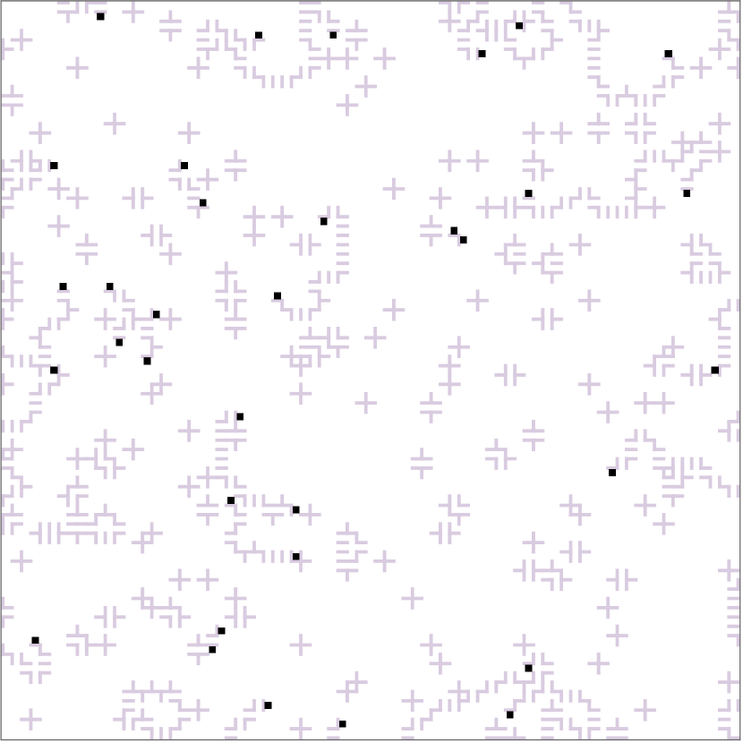
a

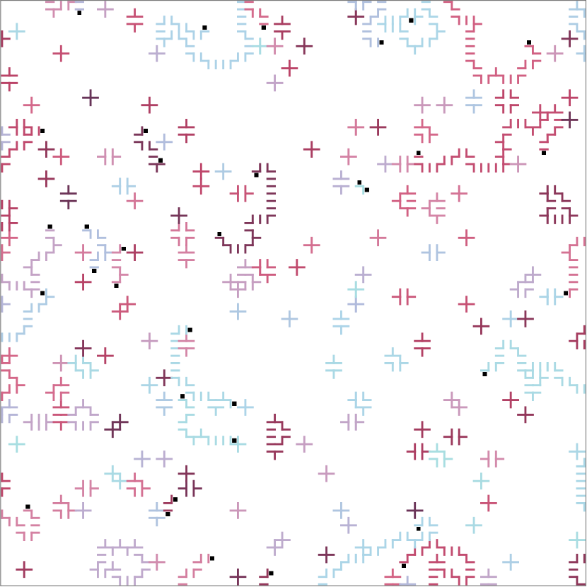
b

Figure 5. This figure shows a gauge field configuration $\sigma$ obtained by simulation of a fixed length lattice Higgs model on a subset of $\mathbb{Z}^{2}$, using $G=\mathbb{Z}_{2}$, free boundary conditions, $\beta=2.2$ and $\kappa=0.48$. In the figures, the colored edges correspond to edges $e$ with $\sigma_{e}=1$ and the black squares to plaquettes $p$ with $(d\sigma)_{p}=1.$ In 5b, we have colored the supports of distinct irreducible gauge field configurations $\sigma^{\prime}\leqslant\sigma$ using different colors.

2.3. Existence of the infinite volume limit

In this section, we recall a result which shows existence and translation invariance of the infinite volume limit $\langle W_{\gamma}\rangle_{\beta,\kappa}$ defined in (1.6) of the expectation of Wilson loop observables. This result is well-known, and is often mentioned in the literature as a direct consequence of the Ginibre inequalities [20]. A full proof of this result in the special case $\kappa=0$ was included in [16], and the general case can be proven completely analogously, hence we omit the proof here.

Proposition 2.26.

Let $G=\mathbb{Z}_{n}$, $M\geqslant 1$, and let $f\colon\Sigma_{E_{M}}\to\mathbb{R}$. For $M^{\prime}\geqslant M$, we abuse notation and let $f$ denote the natural extension of $f$ to $E_{M^{\prime}}$ (i.e., the unique function such that $f(\sigma)=f(\sigma|_{E_{M}})$ for all $\sigma\in\Sigma_{E_{M^{\prime}}}$). Further, let $\beta\in[0,\infty]$ and $\kappa\geqslant 0$. Then the following hold.

1. The limit $\lim_{N\to\infty}\mathbb{E}_{N,\beta,\kappa}\bigl{[}f(\sigma)\bigr{]}$ exists.

2. For any translation $\tau$ of $\mathbb{Z}^{m}$, we have $\lim_{N\to\infty}\mathbb{E}_{N,\beta,\kappa}\bigl{[}f\circ\tau(\sigma)\bigr{]}=\lim_{N\to\infty}\mathbb{E}_{N,\beta,\kappa}\bigl{[}f(\sigma)\bigr{]}$.

2.4. Notation and standing assumptions

In the remainder of the paper, we will assume that ${G=\mathbb{Z}_{n}}$ for some integer $n\geqslant 2$. We will also assume that $\rho\colon G\to\mathbb{C}$ is a unitary, faithful, and one-dimensional representation of $G$. Any such representation has the form $j\mapsto e^{i\cdot j\cdot p\cdot 2\pi/n}$ for some integer $p\in\{0,1,\ldots,n-1\}$ which is relatively prime to $n$. Moreover, we will assume that the Higgs field has fixed length, i.e., we will work with the measure as defined in (1.3). Except in Section 12, we will assume that some integer $N\geqslant 1$ has been fixed.

3. Vortices

In this section, we use the notion of irreducibility introduced in Section 2.1.14 to define what we refer to as vortices. Vortices will play a central role in this paper. We mention that the definition of a vortex given in Definition 3.1 below is identical to the definition used in [16], but is different from the corresponding definitions in [6] and [9].

Definition 3.1 (Vortex).

Let $\sigma\in\Sigma_{E_{N}}$. A non-trivial and irreducible plaquette configuration $\nu\in\Sigma_{P_{N}}$ is said to be a vortex in $\sigma$ if $\nu\leqslant d\sigma$, i.e., if $(d\sigma)_{p}=\nu_{p}$ for all $p\in\operatorname{supp}\nu$.

We say that $\sigma\in\Sigma_{E_{N}}$ has a vortex at $V\subseteq P_{N}$ if $(d\sigma)|_{V}$ is a vortex in $\sigma$. With Lemma 2.17 in mind, we say that a vortex $\nu$ is a minimal vortex if there is $p\in\operatorname{supp}\nu$ with $\hat{\partial}\partial\nu\subseteq P_{N},$ and $|\operatorname{supp}\nu|=12$.

Lemma 3.2.

Let $\sigma\in\Sigma_{E_{N}}$, and let $\nu\in\Sigma_{P_{N}}$ be a minimal vortex in $\sigma$ such that $\hat{\partial}\partial\operatorname{supp}\nu\subseteq P_{N}$. Then there is an edge $e_{0}\in E_{N}$ and a $g\in G\smallsetminus\{0\}$ such that

$$\nu=d\bigl{(}g\mathbb{1}_{e=e_{0}}-g\mathbb{1}_{e=-e_{0}}\bigr{)}.$$ (3.1)

In particular, $(d\sigma)_{p}=\nu_{p}=g$ for all $p\in\hat{\partial}e_{0}$.

Proof.

Let $e_{0}\in E_{N}$ be such that $\operatorname{supp}\nu=\hat{\partial}e_{0}\cup\hat{\partial}(-e_{0})$ (such an $e_{0}$ is guaranteed to exist by Lemma 2.17(ii)). Assume for contradiction that there is no $g\in G\smallsetminus\{0\}$ such that (3.1) holds. Then, since ${\operatorname{supp}\nu=\hat{\partial}e_{0}\cup\hat{\partial}(-e_{0})}$, there exists a $3$-cell $c$ and two plaquettes $p_{1},p_{2}\in\operatorname{supp}\nu\cap\partial c$ with $e_{0}\in p_{1}$ and $-e_{0}\in p_{2}$ such that $\nu_{p_{1}}\neq-\nu_{p_{2}}.$ Since any $3$-cell contains at most two plaquettes in $\hat{\partial}e_{0}\cup\hat{\partial}(-e_{0})$, it follows that

$$\sum_{p\in\partial c}\nu_{p}=\nu_{p_{1}}+\nu_{p_{2}}\neq 0.$$

Using that $\nu=d\sigma^{\prime}$ for some $\sigma^{\prime}\in\Sigma_{E_{N}}$ by Lemma 2.2, this contradicts Lemma 2.1, and hence (3.1) must hold. As a direct consequence, it follows that $(d\sigma)_{p}=\nu_{p}=g$ for $p\in\hat{\partial}e_{0}$. ∎

If $\sigma\in\Sigma_{E_{N}}$ and $\nu\in\Sigma_{P_{N}}$ is a minimal vortex in $\sigma$ which can be written as in (3.1) for some $e_{0}\in E_{N}$ and $g\in G\backslash\{0\}$, then we say that $\nu$ is a minimal vortex centered at $e_{0}$.

Lemma 3.3.

Let $q$ be an oriented surface with boundary $B_{q}$, and let $e_{0}$ be an internal edge of $q$. Further, let $\sigma\in\Sigma_{E_{N}}$, and let $\nu\in\Sigma_{P_{N}}$ be a minimal vortex in $\sigma$, centered at $e_{0}$. Then

$$\sum_{p\in\operatorname{supp}\nu}q_{p}^{+}\nu_{p}=0.$$

Proof.

Since $\nu$ is a vortex centered at $e_{0}$, there is a $g\in G\smallsetminus\{0\}$ such that if we for $e\in E_{N}$ define $\sigma_{e}\coloneqq g\mathbb{1}_{e=e_{0}}-g\mathbb{1}_{e=-e_{0}},$ then $\nu=d\sigma$. By Lemma 2.14, it follows that

$$\sum_{p\in\operatorname{supp}\nu}q_{p}^{+}\nu_{p}=\sum_{p\in P_{N}}q_{p}^{+}\nu_{p}=\sum_{p\in P_{N}}q_{p}^{+}(d\sigma)_{p}=\sum_{e\in B_{q}}\sigma_{e}.$$ (3.2)

Since $e_{0}$ is an internal edge of $q$, we have $\{e_{0},-e_{0}\}\cap B_{q}=\emptyset$. Since $\operatorname{supp}\sigma=\{e_{0},-e_{0}\}$, it follows that the right-hand side of (3.2) vanishes. ∎

The next lemma is a version of Lemma 3.3, valid for general vortices.

Lemma 3.4 (Lemma 5.4 in [16]).

Let $\sigma\in\Sigma_{E_{N}}$, and let $\nu\in\Sigma_{P_{N}}$ be a vortex in $\sigma$. Let $q$ be an oriented surface. If there is a box $B$ containing $\operatorname{supp}\nu$ such that $(*\!*\!B)\cap\operatorname{supp}q$ consists of only internal plaquettes of $q$, then

$$\sum_{p\in P_{N}}q^{+}_{p}\nu_{p}=0.$$ (3.3)

Lemma 3.5.

Let $\sigma\in\Sigma_{E_{N}}$, and let $\nu$ be a vortex in $\sigma$. Then $d\sigma-\nu\in\Sigma_{P_{N}}$.

Proof.

Since $\nu$ is a vortex in $\sigma$, we have $\nu\in\Sigma_{P_{N}}$, and hence $d\nu=0$. Consequently, we have $d(d\sigma-\nu)=dd\sigma-d\nu=0-0=0$, and hence $d\sigma-\nu\in\Sigma_{P_{N}}$. ∎

Before ending this section, we state and prove two lemmas which give connections between vortices in a given gauge field configuration $\sigma$ and in a gauge field configuration $\sigma^{\prime}\leqslant\sigma$.

Lemma 3.6.

Let $\sigma^{\prime},\sigma\in\Sigma_{E_{N}}$ be such that $\sigma^{\prime}\leqslant\sigma$, and let $\nu\in\Sigma_{P_{N}}$ be a vortex in $\sigma^{\prime}$. Then $\nu$ is a vortex in $\sigma$.

Proof.

Assume that $p\in\operatorname{supp}\nu$. Since $\nu$ is a vortex in $\sigma^{\prime}$, we have $(d\sigma^{\prime})_{p}=\nu_{p}\neq 0$, and hence $p\in\operatorname{supp}d\sigma^{\prime}$. Since $\sigma^{\prime}\leqslant\sigma$ and $p\in\operatorname{supp}d\sigma^{\prime},$ it follows from the definition of $\leqslant$ that

$$(d\sigma)_{p}=((d\sigma)|_{\operatorname{supp}d\sigma^{\prime}})_{p}=(d\sigma^{\prime})_{p}=\nu_{p}$$

Since this holds for all $p\in\operatorname{supp}\nu$, $\nu$ is a vortex is $\sigma$. ∎

Lemma 3.7.

Let $\sigma\in\Sigma_{E_{N}}$ and let $\nu\in\Sigma_{P_{N}}$ be a vortex in $\sigma$. Then there is $\sigma^{\prime}\leqslant\sigma$ such that

1. $\nu\leqslant d\sigma^{\prime}$, and

2. there is no $\sigma^{\prime\prime}<\sigma^{\prime}$ such that $\nu\leqslant d\sigma^{\prime\prime}$.

Proof.

Since $\nu$ is a vortex in $\sigma$, we have $\nu\leqslant d\sigma$. Let $\Omega\coloneqq\{\omega\in\Sigma_{E_{N}}\colon\nu\leqslant d\omega\}$. Since $\Sigma_{E_{N}}$ is a finite set and $\Omega\subseteq\Sigma_{E_{N}}$, $\bigl{|}\Omega\bigr{|}$ is finite. The desired conclusion thus follows immediately from applying Lemma 2.8 with $k=1$. ∎

4. Activity of gauge field configurations

In this section, we use the function $\varphi_{r}$, introduced in (1.9), to define the so-called activity of a spin configuration. To this end, recall that for $r\in[0,\infty]$ and $g\in G$, we have defined

$$\varphi_{r}(g)=\begin{cases}e^{r\Re(\rho(g)-\rho(0))}&\text{if }r<\infty,\\ \mathbb{1}_{g=0}&\text{if }r=\infty.\end{cases}$$

Since $\rho$ is a unitary representation of $G$, for any $g\in G$ we have $\rho(g)=\overline{\rho(-g)}$, and hence $\Re\rho(g)=\Re\rho(-g)$. In particular, this implies that for any $g\in G$ and any $r\geqslant 0$, we have

$$\varphi_{r}(g)=e^{r(\Re\rho(g)-\rho(0))}=e^{r\beta(\Re\rho(-g)-\rho(0))}=\varphi_{r}(-g).$$ (4.1)

Clearly, we also have $\varphi_{\infty}(g)=\varphi_{\infty}(-g)$ for all $g\in G$. Moreover, if $a\geqslant 0$ and $r\geqslant 0$, then

$$\varphi_{r}(g)^{a}=\varphi_{ar}(g).$$

Abusing notation, for $\sigma\in\Sigma_{E_{N}}$ and $r\in[0,\infty]$, we let

$$\varphi_{r}(\sigma)\coloneqq\prod_{e\in E_{N}}\varphi_{r}(\sigma_{e}),$$

and for $\omega\in\Sigma_{P_{N}}$ we let

$$\varphi_{r}(\omega)\coloneqq\prod_{p\in P_{N}}\varphi_{r}(\omega_{p}).$$

In analogy with [4], for $\beta\in[0,\infty]$ and $\kappa\geqslant 0$, we define the activity of $\sigma\in\Sigma_{E_{N}}$ by

$$\varphi_{\beta,\kappa}(\sigma)\coloneqq\varphi_{\kappa}(\sigma)\varphi_{\beta}(d\sigma)=\prod_{e\in E_{N}}\varphi_{\kappa}(\sigma_{e})\prod_{p\in P_{N}}\varphi_{\beta}\bigl{(}(d\sigma)_{p}\bigr{)}.$$

Note that with this notation, for $\sigma\in\Sigma_{E_{N}}$, $\beta\in[0,\infty]$, and $\kappa\geqslant 0$, we have

$$\mu_{N,\beta,\kappa}(\sigma)=\frac{\varphi_{\beta,\kappa}(\sigma)}{\sum_{\sigma^{\prime}\in\Sigma_{E_{N}}}\varphi_{\beta,\kappa}(\sigma^{\prime})}.$$ (4.2)

When $\beta=\infty,$ we have $\varphi_{\infty,\kappa}(\sigma)=\varphi_{\kappa}(\sigma)$ if $\sigma\in\Sigma_{E_{N}}^{0}$ and $\varphi_{\infty,\kappa}(\sigma)=0$ if $\sigma\in\Sigma_{E_{N}}\smallsetminus\Sigma_{E_{N}}^{0}.$ Hence, if $\sigma\in\Sigma_{E_{N}},$ then

$$\mu_{N,\infty,\kappa}(\sigma)=\frac{\varphi_{\kappa}(\sigma)\cdot\mathbf{1}_{\sigma\in\Sigma_{E_{N}}^{0}}}{\sum_{\sigma^{\prime}\in\Sigma_{E_{N}}^{0}}\varphi_{\kappa}(\sigma^{\prime})}.$$ (4.3)

The next lemma, which extends Lemma 2.6 in [14] from the case $\kappa=0$ (see also Lemma 3.2.3 in [6]), gives a useful factorization property of $\varphi_{\beta,\kappa}$.

Lemma 4.1.

Let $\sigma,\sigma^{\prime}\in\Sigma_{E_{N}}$ be such that $\sigma^{\prime}\leqslant\sigma$, let $\beta\in[0,\infty]$, and let $\kappa\geqslant 0$. Then

$$\varphi_{\beta,\kappa}(\sigma)=\varphi_{\beta,\kappa}(\sigma^{\prime})\varphi_{\beta,\kappa}(\sigma-\sigma^{\prime}).$$ (4.4)

Proof.

To simplify notation, let $E\coloneqq\operatorname{supp}\sigma^{\prime}$ and $P\coloneqq\operatorname{supp}d\sigma^{\prime}$. Note that

$$\begin{split}&\varphi_{\beta,\kappa}(\sigma)=\prod_{p\in P_{N}}\varphi_{\beta}\bigl{(}(d\sigma)_{p}\bigr{)}\prod_{e\in E_{N}}\varphi_{\kappa}(\sigma_{e})\\ &\qquad=\biggl{[}\,\prod_{p\in P}\varphi_{\beta}\bigl{(}(d\sigma)_{p}\bigr{)}\prod_{e\in E}\varphi_{\kappa}(\sigma_{e})\biggr{]}\cdot\biggl{[}\,\prod_{p\in P_{N}\smallsetminus P}\varphi_{\beta}\bigl{(}(d\sigma)_{p}\bigr{)}\prod_{e\in E_{N}\smallsetminus E}\varphi_{\kappa}(\sigma_{e})\biggr{]}.\end{split}$$ (4.5)

We now make the following observations.

1. Since $\sigma^{\prime}\leqslant\sigma$, for $e\in E$ we have $\sigma_{e}=\sigma^{\prime}_{e}$. On the other hand, since $E=\operatorname{supp}\sigma^{\prime}$, if $e\in E_{N}\smallsetminus E$, then $\sigma^{\prime}_{e}=0$. Since $\varphi_{\kappa}(0)=1$, it follows that

   $$\prod_{e\in E}\varphi_{\kappa}(\sigma_{e})=\prod_{e\in E}\varphi_{\kappa}(\sigma^{\prime}_{e})=\prod_{e\in E_{N}}\varphi_{\kappa}(\sigma^{\prime}_{e}).$$ (4.6)

2. Since $\sigma^{\prime}\leqslant\sigma$, for $e\in E$ we have $\sigma_{e}=\sigma^{\prime}_{e}$, and hence

   $$(\sigma-\sigma^{\prime})_{e}=\sigma_{e}-\sigma^{\prime}_{e}=\sigma^{\prime}_{e}-\sigma^{\prime}_{e}=0.$$

   On the other hand, if $e\in E_{N}\smallsetminus E$, then $\sigma_{e}^{\prime}=0$, and hence

   $$\sigma_{e}=\sigma_{e}-0=\sigma_{e}-\sigma^{\prime}_{e}=(\sigma-\sigma^{\prime})_{e}.$$

   Since $\varphi_{\kappa}(0)=1$, it follows that

   $$\prod_{e\in E_{N}\smallsetminus E}\varphi_{\kappa}(\sigma_{e})=\prod_{e\in E_{N}\smallsetminus E}\varphi_{\kappa}\bigl{(}(\sigma-\sigma^{\prime})_{e}\bigr{)}=\prod_{e\in E_{N}}\varphi_{\kappa}\bigl{(}(\sigma-\sigma^{\prime})_{e}\bigr{)}.$$ (4.7)

3. Since $\sigma^{\prime}\leqslant\sigma$ and $P=\operatorname{supp}d\sigma^{\prime}$, for $p\in P$ we have $(d\sigma)_{p}=(d\sigma^{\prime})_{p}$, and for $p\in P_{N}\smallsetminus P$ we have $(d\sigma^{\prime})_{p}=0$. Consequently, since $\varphi_{\beta}(0)=1$, we have

   $$\prod_{p\in P}\varphi_{\beta}\bigl{(}(d\sigma)_{p}\bigr{)}=\prod_{p\in P}\varphi_{\beta}\bigl{(}(d\sigma^{\prime})_{p}\bigr{)}=\prod_{p\in P_{N}}\varphi_{\beta}\bigl{(}(d\sigma^{\prime})_{p}\bigr{)}.$$ (4.8)

4. Since $P=\operatorname{supp}d\sigma$, if $p\in P_{N}\smallsetminus P$, then $(d\sigma^{\prime})_{p}=0$, and hence

   $$(d\sigma)_{p}=(d\sigma)_{p}-0=(d\sigma)_{p}-(d\sigma^{\prime})_{p}=(d\sigma-d\sigma^{\prime})_{p}=\bigl{(}d(\sigma-\sigma^{\prime})\bigr{)}_{p}.$$

   On the other hand, if $p\in P$, then $(d\sigma^{\prime})_{p}=(d\sigma)_{p}$, and hence

   $$(d(\sigma-\sigma^{\prime}))_{p}=(d\sigma-d\sigma^{\prime})_{p}=(d\sigma)_{p}-(d\sigma^{\prime})_{p}=(d\sigma^{\prime})_{p}-(d\sigma^{\prime})_{p}=0.$$

   Combining these observations and using that $\varphi_{\beta}(0)=1$, we obtain

   $$\prod_{p\in P_{N}\smallsetminus P}\varphi\bigl{(}(d\sigma)_{p}\bigr{)}=\prod_{p\in P_{N}\smallsetminus P}\varphi\bigl{(}(d(\sigma-\sigma^{\prime}))_{p}\bigr{)}=\prod_{p\in P_{N}}\varphi\bigl{(}(d(\sigma-\sigma^{\prime}))_{p}\bigr{)}.$$ (4.9)

Using (4.6), (4.7), (4.8), and (4.9) to substitute the corresponding factors in (4.5), we obtain

$$\begin{split}&\varphi_{\beta,\kappa}(\sigma)=\biggl{[}\,\prod_{p\in P_{N}}\varphi_{\beta}\bigl{(}(d\sigma^{\prime})_{p}\bigr{)}\prod_{e\in E_{N}}\varphi_{\kappa}(\sigma^{\prime}_{e})\biggr{]}\cdot\biggl{[}\,\prod_{p\in P_{N}}\varphi_{\beta}\bigl{(}(d(\sigma-\sigma^{\prime}))_{p}\bigr{)}\prod_{e\in E_{N}}\varphi_{\kappa}((\sigma-\sigma^{\prime})_{e})\biggr{]}\\ &\qquad=\varphi_{\beta,\kappa}(\sigma^{\prime})\varphi_{\beta,\kappa}(\sigma-\sigma^{\prime})\end{split}$$

as desired. ∎

5. Distribution of vortices and gauge field configurations

In this section, we state and prove two propositions. The first proposition estimates the probability that a gauge field configuration $\sigma$ locally agrees with another given gauge field configuration $\sigma^{\prime}$. The second proposition estimates the probability that $d\sigma$ locally agrees with a given irreducible plaquette configuration $\nu$.

Proposition 5.1.

Let $\sigma^{\prime}\in\Sigma_{E_{N}}$, let $\beta\in[0,\infty]$, and let $\kappa\geqslant 0$. Then

$$\mu_{N,\beta,\kappa}\bigl{(}\{\sigma\in\Sigma_{E_{N}}\colon\sigma^{\prime}\leqslant\sigma\}\bigr{)}\leqslant\varphi_{\beta,\kappa}(\sigma^{\prime}).$$

Proof.

Define

$$\Sigma^{\sigma^{\prime}}\coloneqq\{\sigma\in\Sigma_{E_{N}}\colon\sigma^{\prime}\leqslant\sigma\}\quad\text{and}\quad\bar{\Sigma}^{\sigma^{\prime}}\coloneqq\{\sigma\in\Sigma_{E_{N}}\colon\sigma+\sigma^{\prime}\in\Sigma^{\sigma^{\prime}}\}.$$

Using (4.2), and that $\bar{\Sigma}^{\sigma^{\prime}}\subseteq\Sigma_{E_{N}}$, we obtain

$$\mu_{N,\beta,\kappa}\bigl{(}\{\sigma\in\Sigma_{E_{N}}\colon\sigma^{\prime}\leqslant\sigma\}\bigr{)}=\mu_{N,\beta,\kappa}(\Sigma^{\sigma^{\prime}})=\frac{\sum_{\sigma\in\Sigma^{\sigma^{\prime}}}\varphi_{\beta,\kappa}(\sigma)}{\sum_{\sigma\in\Sigma_{E_{N}}}\varphi_{\beta,\kappa}(\sigma)}\leqslant\frac{\sum_{\sigma\in\Sigma^{\sigma^{\prime}}}\varphi_{\beta,\kappa}(\sigma)}{\sum_{\sigma\in\bar{\Sigma}^{\sigma^{\prime}}}\varphi_{\beta,\kappa}(\sigma)}.$$ (5.1)

If $\sigma\in\Sigma^{\sigma^{\prime}}$, then $\sigma^{\prime}\leqslant\sigma$, and hence, by Lemma 4.1, $\varphi_{\beta,\kappa}(\sigma)=\varphi_{\beta,\kappa}(\sigma^{\prime})\varphi_{\beta,\kappa}(\sigma-\sigma^{\prime})$. On the other hand, the mapping $\sigma\mapsto\sigma-\sigma^{\prime}$ is a bijection from $\Sigma^{\sigma^{\prime}}$ to $\bar{\Sigma}^{\sigma^{\prime}}$. Combining these observations, we obtain

$$\sum_{\sigma\in\Sigma^{\sigma^{\prime}}}\varphi_{\beta,\kappa}(\sigma)=\sum_{\sigma\in\Sigma^{\sigma^{\prime}}}\varphi_{\beta,\kappa}(\sigma^{\prime})\varphi_{\beta,\kappa}(\sigma-\sigma^{\prime})=\varphi_{\beta,\kappa}(\sigma^{\prime})\sum_{\sigma\in\Sigma^{\sigma^{\prime}}}\varphi_{\beta,\kappa}(\sigma-\sigma^{\prime})=\varphi_{\beta,\kappa}(\sigma^{\prime})\sum_{\sigma\in\bar{\Sigma}^{\sigma^{\prime}}}\varphi_{\beta,\kappa}(\sigma).$$

This shows that the right-hand side of (5.1) is equal to $\varphi_{\beta,\kappa}(\sigma^{\prime})$, and hence the desired conclusion follows. ∎

The next proposition gives a version of Proposition 5.1 for plaquette configurations.

Proposition 5.2.

Let $\nu\in\Sigma_{P_{N}}$ be irreducible and non-trivial, and assume that $\beta\geqslant 0$ and $\kappa\geqslant 0$ are such that [A1] holds. Then

$$\mu_{N,\beta,\kappa}\bigl{(}\{\sigma\in\Sigma_{E_{N}}\colon\nu\leqslant d\sigma\}\bigr{)}\leqslant\frac{\varphi_{\beta}(\nu)\,\bigl{(}4\alpha_{0}(\kappa)\bigr{)}^{m_{0}}}{1-\alpha_{1}(\beta)-4\alpha_{0}(\kappa)},$$

where

$$m_{0}\coloneqq\frac{1}{2}\min\bigl{\{}|\operatorname{supp}\sigma|\colon\sigma\in\Sigma_{E_{N}}\text{ and }\nu\leqslant d\sigma\bigr{\}}.$$ (5.2)

Before giving a proof of Proposition 5.2, we state and prove three lemmas which we will need. The first of these lemmas will be used to enumerate all gauge field configurations $\sigma\in\Sigma_{E_{N}}$ with $\nu\leqslant d\sigma$ that are minimal in the sense of Lemma 3.7. In this lemma, we associate two different sequences to a vortex $\nu$ in an irreducible edge configuration $\hat{\sigma}$: the first sequence is a sequence of edge configurations $\sigma^{(0)},\sigma^{(1)},\ldots,\sigma^{(m)}\in\Sigma_{E_{N}}$ with increasing supports such that $\sigma^{(0)}=0$ and $\sigma^{(m)}=\hat{\sigma}$, and the second sequence is an increasing sequence of subsets $L_{0}\subseteq L_{1}\subseteq\dots\subseteq L_{m}$ of $P_{N}$ such that $L_{0}=\emptyset$ and $L_{m}=\operatorname{supp}d\hat{\sigma}\smallsetminus\operatorname{supp}\nu$. Together these two sequences can be thought of as a step-wise joint exploration process of $\hat{\sigma}$ and $\operatorname{supp}\hat{\sigma}\smallsetminus\operatorname{supp}\nu$.

Lemma 5.3.

Let $\nu\in\Sigma_{P_{N}}$, and let $\hat{\sigma}\in\Sigma_{E_{N}}$ be such that

1. $\nu$ is a vortex in $\hat{\sigma}$, and

2. there is no $\sigma^{\prime}\in\Sigma_{E_{N}}$ with $\sigma^{\prime}<\hat{\sigma}$ such that $\nu$ is a vortex in $\sigma^{\prime}$.

Assume that an arbitrary total ordering of the plaquettes in $P_{N}$ is given, and define

$$m\coloneqq m(\hat{\sigma},\nu)\coloneqq\bigl{(}|\operatorname{supp}d\hat{\sigma}\smallsetminus\operatorname{supp}\nu|+|\operatorname{supp}\hat{\sigma}|\bigr{)}/2.$$

Then there are sequences $\sigma^{(0)},\sigma^{(1)},\ldots,\sigma^{(m)}\in\Sigma_{E_{N}}$ and $L_{0},L_{1},L_{2},\ldots,L_{m}\subseteq P_{N}$, such that the following properties hold.

1. $\sigma^{(0)}\equiv 0$ and $\sigma^{(m)}=\hat{\sigma}$.

2. $L_{0}=\emptyset$ and $L_{m}=\operatorname{supp}d\hat{\sigma}\smallsetminus\operatorname{supp}\nu$.

Moreover, for all $j\in\{1,2,\ldots,m\}$,

1. if $p\in L_{j}$, then $\sigma^{(j)}_{e}=\hat{\sigma}_{e}$ for all $e\in\partial p$,

2. $\hat{\sigma}|_{\operatorname{supp}\sigma^{(j)}}=\sigma^{(j)}$, and

3. $L_{j}\subseteq\operatorname{supp}d\hat{\sigma}\smallsetminus\operatorname{supp}\nu$.

Further, for $j=1,2,\ldots,m$, let

$$P^{j}\coloneqq\bigl{\{}p\in P_{N}\smallsetminus L_{j-1}\colon(d\sigma^{(j-1)})_{p}\neq\nu_{p}\bigr{\}},$$ (5.3)

and let $p_{j}$ be the plaquette in $P^{j}$ which appears first in the given ordering of the plaquettes. Then $p_{j}$ is well defined, and we can choose the sequences $\sigma^{(0)},\sigma^{(1)},\ldots,\sigma^{(m)}$ and $L_{0},L_{1},\ldots,L_{m}$ such that either

1. $\operatorname{supp}\sigma^{(j)}=\operatorname{supp}\sigma^{(j-1)}\cup\{e_{j},-e_{j}\}$ for some $e_{j}\in\partial p_{j}$, and $L_{j}=L_{j-1}$, or

1. $L_{j}=L_{j-1}\cup\{p_{j},-p_{j}\}$ and $\operatorname{supp}\sigma^{(j)}=\operatorname{supp}\sigma^{(j-1)},$

for $j=1,2,\dots,m$. Moreover, if the plaquettes in $\operatorname{supp}\nu$ occur first in the ordering of the plaquettes, then

1. $L_{0}=L_{1}=\ldots=L_{m_{0}}=\emptyset,$

where $m_{0}$ is given by (5.2).

For $j=1,2,\ldots,m$, we think of the plaquettes in the set $L_{j-1}$ as being “locked” or “frozen” at step $j$.

In Figure 6 and Figure 7, we give examples of sequences $\sigma^{(0)},\sigma^{(1)},\ldots$ and $L_{0},L_{1},\ldots$ which correspond to some given $\hat{\sigma}\in\Sigma_{E_{N}}$ and $\nu\in\Sigma_{P_{N}}$ as in Lemma 5.3.

Proof of Lemma 5.3.

We will show that the conclusion of Lemma 5.3 holds by constructing two sequences $\sigma^{(0)},\sigma^{(1)},\ldots,\sigma^{(m)}\in\Sigma_{E_{N}}$ and $L_{0},L_{1},\ldots,L_{m}\subseteq P_{N}$ with the desired properties. Define $\sigma^{(0)}\equiv 0$ and $L_{0}\coloneqq\emptyset$. Fix $k\in\{1,2,\ldots,m\}$, and assume that $\sigma^{(1)},\ldots,\sigma^{(k-1)}\in\Sigma_{E_{N}}$ and $L_{1},\ldots,L_{k-1}\subseteq P_{N}$ are such that for each $j\in\{0,1,2,\ldots,k-1\}$, (iii), (iv), (v) and either (vi’) or (vi”) holds. Before we construct $\sigma^{(k)}$ and $L_{k}$, we show that these assumptions together imply that the following claim holds.

Claim 5.4.

$p_{k}$ is well defined.

Proof of claim.

Assume for contradiction that $P^{k}=\emptyset$. By the definition of $P^{k}$ (see (5.3)), it follows that $(d\sigma^{(k-1)})_{p}=\nu_{p}$ for all $p\in P_{N}\smallsetminus L_{k-1}$. Since $L_{k-1}\cap\operatorname{supp}\nu=\emptyset$ by (v), we have $(d\sigma^{(k-1)})_{p}=\nu_{p}$ for all $p\in\operatorname{supp}\nu$. Hence $\nu$ is a vortex in $\sigma^{(k-1)}$.

At the same time, if $p\in\operatorname{supp}d\sigma^{(k-1)},$ then either $p\in P_{N}\smallsetminus L_{k-1}$ and $(d\sigma^{(k-1)})_{p}=\nu_{p}=(d\hat{\sigma})_{p}$ (since $\nu$ is a vortex in $\hat{\sigma}$), or $p\in L_{k-1}$, in which case, by (iii), we have $\sigma_{e}^{(k-1)}=\hat{\sigma}_{e}$ for all $e\in\partial p$, and hence $(d\sigma^{(k-1)})_{p}=(d\hat{\sigma})_{p}.$ Consequently, for all $p\in\operatorname{supp}d\sigma^{(k-1)}$ we have $(d\sigma^{(k-1)})_{p}=(d\hat{\sigma})_{p}.$ Since $\sigma^{(k-1)}=\hat{\sigma}|_{\operatorname{supp}\sigma^{(k-1)}}$ by construction, it follows that $\sigma^{(k-1)}\leqslant\hat{\sigma}.$

Since $\sigma^{(k-1)}\leqslant\hat{\sigma}$ and $\nu$ is a vortex in $\sigma^{(k-1)},$ it now follows from (b) that $\sigma^{(k-1)}=\hat{\sigma}$. Since $P^{k}$ is empty by assumption, it follows from the definition of $P^{k}$ that $(d\hat{\sigma})_{p}=\nu_{p}$ for each $p\in P_{N}\smallsetminus L_{k-1}$, and consequently, we have $L_{k-1}=\operatorname{supp}d\hat{\sigma}\smallsetminus\operatorname{supp}\nu$. Since either (vi’) or (vi”) holds for each $j\in\{1,2,\ldots,k-1\}$, we infer that

$$k-1=\bigl{(}|L_{k-1}|+|\operatorname{supp}\sigma^{(k-1)}|\bigr{)}/2=\bigl{(}|\operatorname{supp}d\hat{\sigma}\smallsetminus\operatorname{supp}\nu|+|\operatorname{supp}\hat{\sigma}|\bigr{)}/2,$$ (5.4)

and hence by the definition of $m$, we have $k-1=m$. Since this contradicts that $k\leqslant m$, the set $P^{k}$ must be nonempty, implying in particular that $p_{k}$ is well defined. ∎

We now define $\sigma^{(k)}$ and $L_{k}$.

If $\sigma^{(k-1)}_{e}=\hat{\sigma}_{e}$ for all edges $e\in\partial p_{k}\smallsetminus\partial L_{k-1}$ where $\partial L_{k-1}=\cup_{p\in L_{k-1}}\partial p$, we let $\sigma^{(k)}\coloneqq\sigma^{(k-1)}$ and $L_{k}\coloneqq L_{k-1}\cup\{p_{k},-p_{k}\}$. Then (iii) holds for $j=k$ by assumption, and (vi”) holds for $j=k$ by construction. Since $\sigma^{(k)}=\sigma^{(k-1)}$ and (iv) holds for $j=k-1$ by assumption, (iv) holds with $j=k$. Finally, we show that (v) holds. By (iii) and by the definition of $p_{k}$, $(d\hat{\sigma})_{p_{k}}=(d\sigma^{(k-1)})_{p_{k}}\neq\nu_{p_{k}}$. Thus, since $\nu$ is a vortex in $\hat{\sigma}$, we have $\nu_{p_{k}}=0$, and hence $p_{k}\in\operatorname{supp}d\hat{\sigma}\smallsetminus\operatorname{supp}\nu$. Since $L_{k}=L_{k-1}\cup\{p_{k},-p_{k}\}$, and since (v) holds for $j=k-1$ by assumption, it follows that $L_{k}\subseteq\operatorname{supp}d\hat{\sigma}\smallsetminus\operatorname{supp}\nu$, and thus (v) holds for $j=k$.

On the other hand, if there is an edge $e_{k}\in\partial p_{k}\smallsetminus\partial L_{k-1}$ such that $\sigma^{(k-1)}_{e_{k}}\neq\hat{\sigma}_{e_{k}}$, then let $L_{k}\coloneqq L_{k-1}$ and, for $e\in E_{N}$, define

$$\sigma^{(k)}(e)\coloneqq\begin{cases}\hat{\sigma}_{e}&\text{if }e=\pm e_{k},\cr\sigma^{(k-1)}_{e}&\text{else.}\end{cases}$$

Since $L_{k}=L_{k-1}$, and, since $\sigma^{(k)}$ and $\sigma^{(k-1)}$ differ only at $\pm e_{k}\notin\partial L_{k-1}$, (iii) holds for $j=k$ (since it holds for $j=k-1$ by assumption). Since (iv) holds for $j=k-1$ by assumption, (iv) holds also when $j=k$. By construction, (vi’) holds. Finally, since (v) holds for $j=k-1$ by assumption, we have $L_{k}=L_{k-1}\subseteq\operatorname{supp}d\hat{\sigma}\smallsetminus\operatorname{supp}\nu$, and hence (v) holds also for $j=k$.

To sum up, we have constructed sequences $\sigma^{(0)},\ldots,\sigma^{(k)}\in\Sigma_{E_{N}}$ and $L_{0},\ldots,L_{k}\subseteq P_{N}$ such that, for each $j\in\{1,2,\ldots,k\}$, (iii), (iv), (v), and either (vi’) or (vi”) holds. This completes the inductive step and shows that sequences $\sigma^{(0)},\sigma^{(1)},\ldots,\sigma^{(m)}$ and $L_{0},L_{1},\ldots,L_{m}$ can be defined by repeating the above steps recursively.

We now prove that if $\sigma^{(0)},\sigma^{(1)},\ldots,\sigma^{(m)}$ and $L_{0},L_{1},\ldots,L_{m}$ are defined as above, then ${\sigma^{(m)}=\hat{\sigma}}$.

Claim 5.5.

$\sigma^{(m)}=\hat{\sigma}$ and $L_{m}=\operatorname{supp}d\hat{\sigma}\smallsetminus\operatorname{supp}\nu.$

Proof of claim.

Since either (vi’) or (vi”) holds for each $j\in\{1,2,\ldots,m\}$, we have

$$m=\bigl{(}|L_{m}|+|\operatorname{supp}\sigma^{(m)}|\bigr{)}/2.$$

By definition, we also have

$$m=\bigl{(}|\operatorname{supp}d\hat{\sigma}\smallsetminus\operatorname{supp}\nu|+|\operatorname{supp}\hat{\sigma}|\bigr{)}/2.$$

Since $L_{m}\subseteq\operatorname{supp}d\hat{\sigma}\smallsetminus\operatorname{supp}\nu$ by (v), and $\operatorname{supp}\sigma^{(m)}\subseteq\operatorname{supp}\hat{\sigma}$ by (iv), it follows that $L_{m}=\operatorname{supp}d\hat{\sigma}\smallsetminus\operatorname{supp}\nu$ and $\operatorname{supp}\sigma^{(m)}=\operatorname{supp}\hat{\sigma}$. Again using (iv), it follows that $\sigma^{(m)}=\hat{\sigma}$. ∎

It only remains to prove that (vii) holds.

Claim 5.6.

If the plaquettes in $\operatorname{supp}\nu$ appear first in the ordering of the plaquettes, then $L_{0}=L_{1}=\cdots=L_{m_{0}}=\emptyset$.

Proof of claim.

Assume that the plaquettes in $\operatorname{supp}\nu$ appear first in the ordering of the plaquettes. Furthermore, assume that $k\leqslant m$ is the largest positive integer such that $p_{1},p_{2},\ldots,p_{k}\in\operatorname{supp}\nu$. Since $L_{k}\cap\operatorname{supp}\nu=\emptyset$ by (v), it follows that $L_{0}=L_{1}=\dots=L_{k}=\emptyset$. Consequently, it suffices to show that $k\geqslant m_{0}.$

If $k<m$, then $p_{k+1}\notin\operatorname{supp}\nu$. Since the plaquettes in $\operatorname{supp}\nu$ appear first in the ordering of the plaquettes and $P^{k+1}=\{p\in P_{N}\colon(d\sigma^{(k)})_{p}\neq\nu_{p}\}$, we must have $(d\sigma^{(k)})_{p}=\nu_{p}$ for all $p\in\operatorname{supp}\nu$ by the choice of $p_{k+1}$. On the other hand, if $k=m$, then by (i), we have $\sigma^{(k)}=\sigma^{(m)}=\hat{\sigma}$, and hence $(d\sigma^{(k)})_{p}=(d\hat{\sigma})_{p}=\nu_{p}$ for all $p\in\operatorname{supp}\nu$ also in this case. Since $d\nu=0=d(d\sigma^{(k)})$, if follows that $\nu\leqslant d\sigma^{(k)}$. Consequently, by definition (see (5.2)), we have $|\operatorname{supp}\sigma^{(k)}|\geqslant 2m_{0}$. Since, by construction, $|\operatorname{supp}\sigma^{(k)}|\leqslant|\operatorname{supp}\sigma^{(k-1)}|+2$ and $|\operatorname{supp}\sigma^{(0)}|=0$, it follows that $k\geqslant m_{0}$. This concludes the proof of the claim. ∎

∎

a The gauge field configuration $\hat{\sigma}$.

b $j=0$

c $j=1$

d $j=2$

e $j=3$

f $j=4$

g $j=5$

Figure 6. Assuming that $G=\mathbb{Z}_{2}$, consider the gauge field configuration $\hat{\sigma}$ and plaquette ordering given in Figure 6a above. Note that it contains a (minimal) vortex $\nu$ with support on two plaquettes (dark gray). Figures 6b, 6c, 6d, 6e, 6f, and 6g above correspond to $j=0,1,2,3,4,5$ respectively, and in each picture we draw the vortex $\nu$ (dark gray), the set $P^{j+1}$ (blue), the plaquette $p_{j}$ ($*$), the edge $e_{j}$ (red), and the gauge field configuration $\sigma^{(j)}$ (union of black and red edges) given in the proof of Lemma 5.3, given the ordering of the plaquettes shown in 6a. Note that in this example, we have $L_{j}=\emptyset$ for all $j$. Note also that although in this case, there are no distinct $i$ and $j$ such that $p_{i}=p_{j}$, this is in general not the case when $G\neq\mathbb{Z}_{2}$. Moreover, in general, $e_{j}$ is not always uniquely determined by the previous steps.

a The gauge field configuration $\hat{\sigma}$.

b $j=0$

c $j=1$

d $j=2$

e $j=3$

f $j=4$

g $j=5$

h $j=6$

Figure 7. Assuming that $G=\mathbb{Z}_{2}$, consider the gauge field configuration $\hat{\sigma}$ and plaquette ordering given by Figure 7a above. Note that it contains two (minimal) vortices $\nu_{1}$ (dark gray) and $\nu_{2}$ (light gray), each with support on exactly two plaquettes. Figures 7b, 7c, 7d, 7e, 7f, 7g, and 7h correspond to $j=0,1,2,3,4,5,6$ respectively. In each picture we draw the vortices $\nu=\nu_{1}$ (dark gray), $\nu_{2}$ (light gray), the set $P^{j+1}$ (blue), the plaquette $p_{j}$ ($*$), the edge $e_{j}$ (red), the gauge field configuration $\sigma^{(j)}$ and the set $L_{j}$ (purple) given in the proof of Lemma 5.3, given the ordering of the plaquettes shown in Figure 7a.

Lemma 5.7.

Let $\beta\geqslant 0$ and $\kappa\geqslant 0$. Further, let $\nu\in\Sigma_{P_{N}}$ be irreducible and non-trivial, and define $m_{0}$ by (5.2). For each $m\geqslant 0$, let $\Sigma_{E_{N},\nu,m}$ be the set of all $\sigma^{\prime}\in\Sigma_{E_{N}}$ such that

1. $\nu\leqslant d\sigma^{\prime}$,

2. $\nu\nleq d\sigma^{\prime\prime}$ for any $\sigma^{\prime\prime}<\sigma^{\prime}$, and

3. $|\operatorname{supp}d\sigma^{\prime}\smallsetminus\operatorname{supp}\nu|+|\operatorname{supp}\sigma^{\prime}|=2m$.

Then

$$\begin{split}&\mu_{N,\beta,\kappa}\bigl{(}\{\sigma\in\Sigma_{E_{N}}\colon\nu\leqslant d\sigma\}\bigr{)}\leqslant\sum_{m=m_{0}}^{\infty}\sum_{\sigma^{\prime}\in\Sigma_{E_{N},\nu,m}}\varphi_{\beta,\kappa}(\sigma^{\prime}).\end{split}$$ (5.5)

Proof.

Consider the event $\{\sigma\in\Sigma_{E_{N}}\colon\exists\sigma^{\prime}\in\Sigma_{E_{N},\nu,m}\text{ such that }\sigma^{\prime}\leqslant\sigma\}$. The set $\Sigma_{E_{N},\nu,m}$ is empty if $m<m_{0}$. By Lemma 3.6 and Lemma 3.7, we thus have

$$\begin{split}&\mu_{N,\beta,\kappa}\bigl{(}\{\sigma\in\Sigma_{E_{N}}\colon\nu\text{ is a vortex in }\sigma\}\bigr{)}\\ &\qquad=\mu_{N,\beta,\kappa}\biggl{(}\{\sigma\in\Sigma_{E_{N}}\colon\exists\sigma^{\prime}\in\bigcup_{m=m_{0}}^{\infty}\Sigma_{E_{N},\nu,m}\text{ such that }\sigma^{\prime}\leqslant\sigma\}\biggr{)}\end{split}$$

and hence, by a union bound,

$$\begin{split}&\mu_{N,\beta,\kappa}\bigl{(}\{\sigma\in\Sigma_{E_{N}}\colon\nu\text{ is a vortex in }\sigma\}\bigr{)}\leqslant\sum_{m=m_{0}}^{\infty}\mu_{N,\beta,\kappa}\bigl{(}\{\sigma\in\Sigma_{E_{N}}\colon\exists\sigma^{\prime}\in\Sigma_{E_{N},\nu,m}\text{ such that }\sigma^{\prime}\leqslant\sigma\}\bigr{)}.\end{split}$$

By a union bound, for any $m\geqslant m_{0}$, we have

$$\mu_{N,\beta,\kappa}\bigl{(}\{\sigma\in\Sigma_{E_{N}}\colon\exists\sigma^{\prime}\in\Sigma_{E_{N},\nu,m}\text{ such that }\sigma^{\prime}\leqslant\sigma\}\bigr{)}\leqslant\sum_{\sigma^{\prime}\in\Sigma_{E_{N},\nu,m}}\mu_{N,\beta,\kappa}\bigl{(}\{\sigma\in\Sigma_{E_{N}}\colon\sigma^{\prime}\leqslant\sigma\}\bigr{)}.$$

Since, by Proposition 5.1, for any $\sigma^{\prime}\in\Sigma_{E_{N}}$, we have

$$\mu_{N,\beta,\kappa}\bigl{(}\{\sigma\in\Sigma_{E_{N}}\colon\sigma^{\prime}\leqslant\sigma\}\bigr{)}\leqslant\varphi_{\beta,\kappa}(\sigma^{\prime})$$

we obtain (5.5) as desired. ∎

Lemma 5.8.

Let $\beta\geqslant 0$, and let $\kappa\geqslant 0$. Let $\nu\in\Sigma_{P_{N}}$ be irreducible and non-trivial, and define $m_{0}$ by (5.2). Let $\Sigma_{E_{N},\nu,m}$ be the sets defined in Lemma 5.7. Then, for any $m\geqslant m_{0}$,

$$\begin{split}&\sum_{\hat{\sigma}\in\Sigma_{E_{N},\nu,m}}\varphi_{\beta,\kappa}(\hat{\sigma})\leqslant\varphi_{\beta}(\nu)\,\bigl{(}4\alpha_{0}(\kappa)\bigr{)}^{m_{0}}\Bigl{(}\alpha_{1}(\beta)+4\alpha_{0}(\kappa)\Bigr{)}^{m-m_{0}},\end{split}$$

where $\alpha_{0}$ and $\alpha_{1}$ are defined in (1.11).

Proof.

Let $V\coloneqq\operatorname{supp}\nu$ and assume that $\hat{\sigma}\in\Sigma_{E_{N},\nu,m}$. By definition,

$$\varphi_{\beta,\kappa}(\hat{\sigma})=\biggl{[}\,\prod_{p^{\prime}\in\operatorname{supp}d\hat{\sigma}}\varphi_{\beta}\bigl{(}(d\hat{\sigma})_{p}\bigr{)}\biggr{]}\cdot\biggl{[}\,\prod_{e\in\operatorname{supp}\hat{\sigma}}\varphi_{\kappa}(\hat{\sigma}_{e})\biggr{]}.$$

Using that $(d\hat{\sigma})|_{V}=\nu$ and hence $V\subseteq\operatorname{supp}d\hat{\sigma}$, we obtain

$$\varphi_{\beta,\kappa}(\hat{\sigma})=\varphi_{\beta}(\nu)\biggl{[}\,\prod_{p^{\prime}\in(\operatorname{supp}d\hat{\sigma})\smallsetminus V}\varphi_{\beta}\bigl{(}(d\hat{\sigma})_{p}\bigr{)}\biggr{]}\cdot\biggl{[}\,\prod_{e\in\operatorname{supp}\hat{\sigma}}\varphi_{\kappa}(\hat{\sigma}_{e})\biggr{]}.$$ (5.6)

Next note that the assumptions of Lemma 5.3 are satisfied. Let the integer $m$, the sets $L_{0},L_{1},\ldots,L_{m}$ and the 1-forms $\sigma^{(0)},\sigma^{(1)},\ldots,\sigma^{(m)}$ be as in Lemma 5.3 when applied with $\hat{\sigma}$ and $\nu$. Then the following hold for each $j\in\{1,2,\ldots,m\}$.

1. By (i) of Lemma 5.3, we have $\sigma^{(0)}=0$ and $\sigma^{(m)}=\hat{\sigma}$, and by (ii) of Lemma 5.3, we have $L_{0}=\emptyset$ and $L_{m}=\operatorname{supp}d\hat{\sigma}\smallsetminus\operatorname{supp}\nu$.

2. By (vi’) and (vi”) of Lemma 5.3, either $L_{j}=L_{j-1}$ or $\sigma^{(j)}=\sigma^{(j-1)}$ (but not both).

3. By (vi’) and (vi”) of Lemma 5.3, if $L_{j}\neq L_{j-1}$, then there is a plaquette $p_{j}\in\operatorname{supp}d\hat{\sigma}\smallsetminus V$ such that $L_{j}=L_{j-1}\sqcup\{p_{j},-p_{j}\}$.

4. By (vi’) and (vi”) of Lemma 5.3, if $\sigma^{(j)}\neq\sigma^{(j-1)}$, then there is an edge $e_{j}\in\operatorname{supp}\hat{\sigma}\smallsetminus\operatorname{supp}\sigma^{(j-1)}$ such that $\sigma^{(j)}_{e^{\prime}}=\sigma^{(j-1)}_{e^{\prime}}+\hat{\sigma}_{e^{\prime}}\mathbb{1}_{e^{\prime}=\pm e_{j}}$ for all $e^{\prime}\in E_{N}$.

Together, these observations imply that

$$\begin{split}&\biggl{[}\,\prod_{p^{\prime}\in(\operatorname{supp}d\hat{\sigma})\smallsetminus V}\varphi_{\beta}\bigl{(}(d\hat{\sigma})_{p}\bigr{)}\biggr{]}\cdot\biggl{[}\,\prod_{e\in\operatorname{supp}\hat{\sigma}}\varphi_{\kappa}(\hat{\sigma}_{e})\biggr{]}\\ &\qquad=\prod_{j=1}^{m}\Bigl{[}\mathbb{1}\bigl{(}L_{j}\neq L_{j-1}\bigr{)}\varphi_{\beta}\bigl{(}(d\hat{\sigma})_{p_{j}}\bigr{)}^{2}+\mathbb{1}\bigl{(}{\sigma^{(j)}\neq\sigma^{(j-1)}}\bigr{)}\varphi_{\kappa}(\hat{\sigma}_{e_{j}})^{2}\Bigr{]},\end{split}$$ (5.7)

where $\mathbb{1}(L_{j}\neq L_{j-1})$ is equal to one if $L_{j}\neq L_{j-1}$ and zero otherwise; analogously, $\mathbb{1}(\sigma^{(j)}\neq\sigma^{(j-1)})$ equals one if $\sigma^{(j)}\neq\sigma^{(j-1)}$ and zero otherwise. If $L_{j}\neq L_{j-1}$, then $p_{j}\in\operatorname{supp}d\hat{\sigma}$, and thus $\varphi_{\beta}\bigl{(}(d\hat{\sigma})_{p_{j}}\bigr{)}^{2}\leqslant\alpha_{1}(\beta)$ by the definition (1.11) of $\alpha_{1}$. Consequently, (5.6) and (5.7) yield

$$\varphi_{\beta,\kappa}(\hat{\sigma})\leqslant\varphi_{\beta}(\nu)\prod_{j=1}^{m}\Bigl{[}\mathbb{1}\bigl{(}L_{j}\neq L_{j-1}\bigr{)}\alpha_{1}(\beta)+\mathbb{1}\bigl{(}{\sigma^{(j)}\neq\sigma^{(j-1)}}\bigr{)}\varphi_{\kappa}(\hat{\sigma}_{e_{j}})^{2}\Bigr{]}.$$ (5.8)

Given some $j\in\{1,2,\ldots,m\}$, we now make a few additional observations regarding the above indicator functions.

1. If for each plaquette $p\in P_{N}$, we let $\partial p[1]$, $\partial p[2]$, $\partial p[3]$, and $\partial p[4]$ denote the positively oriented edges in $\partial p$, then by (vi’) of Lemma 5.3 we have

   $$\begin{split}&\mathbb{1}(\sigma^{(j)}\neq\sigma^{(j-1)})\\ &\qquad=\sum_{k\in\{1,2,3,4\}}\sum_{g\in G\smallsetminus\{0\}}\mathbb{1}\bigl{(}\operatorname{supp}\sigma^{(j)}\smallsetminus\operatorname{supp}\sigma^{(j-1)}=\{\partial p_{j}[k],-\partial p_{j}[k]\}\text{ and }\sigma^{(j)}_{\partial p_{j}[k]}=g\bigr{)}.\end{split}$$ (5.9)

2. If we for each $j\in\{1,2,\ldots,m\}$ know which indicator (if any) in the right-hand side of (5.9) is non-zero, then we know $\sigma^{(m)}$. Since $\hat{\sigma}=\sigma^{(m)}$, this fully determines $\hat{\sigma}$.

3. By (vii) of Lemma 5.3, we have $L_{0}=L_{1}=\dots=L_{m_{0}}=\emptyset$.

By combining (5.8) with the above observations, we obtain

$$\begin{split}&\sum_{\hat{\sigma}\in\Sigma_{E_{N},\nu,m}}\varphi_{\beta,\kappa}(\hat{\sigma})\leqslant\varphi_{\beta}(\nu)\Bigl{[}4\sum_{g\in G\smallsetminus\{0\}}\varphi_{\kappa}(g)^{2}\Bigr{]}^{m_{0}}\prod_{j=m_{0}+1}^{m}\biggl{[}\alpha_{1}(\beta)+4\sum_{g\in G\smallsetminus\{0\}}\varphi_{\kappa}(g)^{2}\biggr{]}\\ &\qquad=\varphi_{\beta}(\nu)\bigl{(}4\alpha_{0}(\kappa)\bigr{)}^{m_{0}}\Bigl{(}\alpha_{1}(\beta)+4\alpha_{0}(\kappa)\Bigr{)}^{m-m_{0}}\end{split}$$

as desired. ∎

Proof of Proposition 5.2.

Let $m_{0}$ be given by (5.2) and let $\Sigma_{E_{N},\nu,m}$ be the sets defined in Lemma 5.7. By Lemma 5.7, we have

$$\begin{split}&\mu_{N,\beta,\kappa}\bigl{(}\{\sigma\in\Sigma_{E_{N}}\colon\nu\text{ is a vortex in }\sigma\}\bigr{)}\leqslant\sum_{m=m_{0}}^{\infty}\sum_{\hat{\sigma}\in\Sigma_{E_{N},\nu,m}}\varphi_{\beta,\kappa}(\hat{\sigma}).\end{split}$$

On the other hand, by Lemma 5.8, for any $m\geqslant m_{0}$, we have

$$\begin{split}&\sum_{\hat{\sigma}\in\Sigma_{E_{N},\nu,m}}\varphi_{\beta,\kappa}(\hat{\sigma})\leqslant\varphi_{\beta}(\nu)\bigl{(}4\alpha_{0}(\kappa)\bigr{)}^{m_{0}}\Bigl{(}\alpha_{1}(\beta)+4\alpha_{0}(\kappa)\Bigr{)}^{m-m_{0}}.\end{split}$$

Combining these two inequalities, we get

$$\begin{split}&\mu_{N,\beta,\kappa}\bigl{(}\{\sigma\in\Sigma_{E_{N}}\colon\nu\text{ is a vortex in }\sigma\}\bigr{)}\leqslant\varphi_{\beta}(\nu)\bigl{(}4\alpha_{0}(\kappa)\bigr{)}^{m_{0}}\sum_{m=m_{0}}^{\infty}\bigl{(}\alpha_{1}(\beta)+4\alpha_{0}(\kappa)\bigr{)}^{m-m_{0}}.\end{split}$$

Since $\alpha_{1}(\beta)+4\alpha_{0}(\kappa)<1$ by assumption [A1], we have

$$\begin{split}&\sum_{j=0}^{\infty}\bigl{(}\alpha_{1}(\beta)+4\alpha_{0}(\kappa)\bigr{)}^{j}=\frac{1}{1-\alpha_{1}(\beta)-4\alpha_{0}(\kappa)},\end{split}$$

we hence obtain

$$\begin{split}&\mu_{N,\beta,\kappa}\bigl{(}\{\sigma\in\Sigma_{E_{N}}\colon\nu\text{ is a vortex in }\sigma\}\Bigr{)}\leqslant\frac{\varphi_{\beta}(\nu)\bigl{(}4\alpha_{0}(\kappa)\bigr{)}^{m_{0}}}{1-\alpha_{1}(\beta)-4\alpha_{0}(\kappa)},\end{split}$$

which is the desired conclusion. ∎

6. Distribution of frustrated plaquettes

In this section we establish an upper bound for the probability that a gauge field configuration contains a large vortex with support containing a given plaquette.

In order to simplify notation, given $\sigma\in\Sigma_{E_{N}}$ and $p\in P_{N}$, we let $(d\sigma)^{p}$ be the set of vortices in $\sigma$ with support containing $p$.

Proposition 6.1 (Compare with Proposition 5.9 in [16]).

Let $\beta\geqslant 0$ and $\kappa\geqslant 0$ be such that [A1] and [A2] hold. Further, let $p_{0}\in P_{N}$ and $M\geqslant 1$. Then

$$\begin{split}&\mu_{N,\beta,\kappa}\bigl{(}\{\sigma\in\Sigma_{E_{N}}\colon\exists\nu\in(d\sigma)^{p_{0}}\text{ with }|\operatorname{supp}\nu|\geqslant 2M\}\bigr{)}\leqslant C_{0}^{(M)}\alpha_{2}(\beta,\kappa)^{\mathrlap{M}},\end{split}$$ (6.1)

where

$$C_{0}^{(M)}\coloneqq\frac{5^{M}4^{M/6}}{\bigl{(}1-\alpha_{1}(\beta)-4\alpha_{0}(\kappa)\bigr{)}\bigl{(}1-2^{1/3}5\alpha_{2}(\beta,\kappa)\bigr{)}}.$$ (6.2)

Before we give a proof of Proposition 6.1, we state and prove the following lemma, which essentially corresponds to the first part of the proof of Proposition 2.11 in [16].

Lemma 6.2.

Let $p_{0}\in P_{N}$, $m\geqslant 1$, and $\beta\geqslant 0$. Let $\Lambda_{m}$ be the set of all irreducible plaquette configurations $\nu\in\Sigma_{P_{N}}$ with $p_{0}\in\operatorname{supp}\nu$ and $|\operatorname{supp}\nu|=2m$. Then

$$\sum_{\nu\in\Lambda_{m}}\varphi_{\beta}(\nu)\leqslant 5^{m-1}\alpha_{0}(\beta)^{m}.$$ (6.3)

Proof.

We will prove the lemma by giving a mapping from $\Lambda_{m}$ to a set of sequences $\nu^{1},\nu^{2},\ldots,\nu^{m}$ of $G$-valued 2-forms on $P_{N}$. To this end, assume that total orderings of the plaquettes and 3-cells in $B_{N}$ are given.

Fix some $\nu\in\Lambda_{m}$. Let $p_{1}=p_{1}(\nu)\coloneqq p_{0}$, and define

$$\nu^{1}(p)\coloneqq\begin{cases}\nu_{p}&\text{if }p=p_{1},\cr-\nu_{p}&\text{if }p=-p_{1},\cr 0&\text{otherwise.}\end{cases}$$

Next, assume that for some $k\in\{1,2,\ldots,m\}$, we are given 2-forms $\nu^{1},\nu^{2},\ldots,\nu^{k}$ such that for each $j\in\{1,2,\ldots,k\}$ we have

1. $\operatorname{supp}\nu^{j}\smallsetminus\operatorname{supp}\nu^{j-1}=\{p_{j},-p_{j}\}$ for some $p_{j}\in P_{N}$, and

2. $\nu|_{\operatorname{supp}\nu^{j}}=\nu^{j}$.

If $d\nu^{k}=0$, then $\nu^{k}\in\Sigma_{P_{N}}$ and, by (b), we have $\nu|_{\operatorname{supp}\nu^{k}}=\nu^{k}$. Since $\nu$ is irreducible by assumption, and $\operatorname{supp}\nu^{k}\neq\emptyset$ by (a), it follows that $\nu^{k}=\nu$. Since $|\operatorname{supp}\nu^{k}|=2k$ by (a), we conclude that $k=m$. Consequently, if $k<m$, then $d\nu^{k}\not\equiv 0$, so there is at least one oriented 3-cell $c\in B_{N}$ for which $(d\nu^{k})_{c}\neq 0$. Let $c_{k+1}$ be the first oriented 3-cell (with respect to the ordering of the 3-cells) for which $(d\nu^{k})_{c_{k+1}}\neq 0$. Since $\nu\in\Sigma_{P_{N}}$, we have $(d\nu)_{c_{k+1}}=0$, and consequently there exists at least one plaquette $p\in\operatorname{supp}\nu\cap\partial c_{k+1}\smallsetminus\operatorname{supp}\nu^{k}.$ Let $p_{k+1}\coloneqq p_{k+1}(\nu)$ be the first such plaquette (with respect to the ordering of the plaquettes) and define

$$\nu^{k+1}(p)\coloneqq\begin{cases}\nu_{p}&\text{if }p=p_{k+1},\cr-\nu_{p}&\text{if }p=-p_{k+1},\cr\nu^{k}(p)&\text{otherwise.}\end{cases}$$

Note that if $\nu^{1},\nu^{2},\ldots,\nu^{k}$ satisfies (a) and (b), then so does $\nu^{k+1}$.

We now show that $\nu^{m}=\nu$. By (a), $|\operatorname{supp}\nu^{m}|=2m$ and by (b), $\nu|_{\operatorname{supp}\nu^{m}}=\nu^{m}$. Since $|\operatorname{supp}\nu|=2m$, it follows that $\nu^{m}=\nu$.

In order to simplify notation, let $[m]\coloneqq\{1,2,\ldots,m\}$. To obtain (6.3), note first that the above mapping allows us to write

$$\sum_{\nu\in\Lambda_{m}}\varphi_{\beta}(\nu)=\sum_{\nu\in\Lambda_{m}}\prod_{j=1}^{m}\varphi_{\beta}\bigl{(}\nu_{p_{j}(\nu)}\bigr{)}^{2}=\sum_{g_{1},g_{2},\ldots,g_{m}\in G\smallsetminus\{0\}}\sum_{\begin{subarray}{c}\nu\in\Lambda_{m}\colon\\ \nu_{p_{j}(\nu)}=g_{j}\,\forall j\in[m]\end{subarray}}\,\prod_{j=1}^{m}\varphi_{\beta}\bigl{(}g_{j}\bigr{)}^{2}.$$

Given a sequence $p_{1},p_{2},\ldots,p_{m}\in P_{N}$ and a sequence $g_{1},\dots,g_{m}\in G\smallsetminus\{0\}$, there is at most one $\nu\in\Lambda_{m}$ with $p_{j}=p_{j}(\nu)$ and $\nu_{p_{j}}=g_{j}$ for all $j\in[m]$. This implies in particular that the right-hand side of the previous equation is equal to

$$\sum_{g_{1},g_{2},\ldots,g_{m}\in G\smallsetminus\{0\}}\sum_{\begin{subarray}{c}p_{1},p_{2},\ldots,p_{m}\in P_{N}\colon\\ \begin{subarray}{c}\exists\nu\in\Lambda_{m}\colon\forall j\in[m]\colon\\ p_{j}=p_{j}(\nu)\text{ and }\nu_{p_{j}}=g_{j}\end{subarray}\end{subarray}}\,\prod_{j=1}^{m}\varphi_{\beta}\bigl{(}g_{j}\bigr{)}^{2}.$$

Given $\nu^{k}$, the 3-cell $c_{k+1}$ is uniquely defined and satisfies $|\partial c_{k+1}\cap\operatorname{supp}\nu^{k}|\geqslant 1.$ Since we always have $p_{k+1}\in\partial c_{k+1}\smallsetminus\operatorname{supp}\nu^{k},$ given $\nu^{k},$ there can be at most five possible choices for $p_{k+1}$. Since $p_{1}=p_{0}$ by construction, this implies in particular that

$$\sum_{g_{1},g_{2},\ldots,g_{m}\in G\smallsetminus\{0\}}\sum_{\begin{subarray}{c}p_{1},p_{2},\ldots,p_{m}\in P_{N}\colon\\ \begin{subarray}{c}\exists\nu\in\Lambda_{m}\colon\forall j\in[m]\colon\\ p_{j}=p_{j}(\nu)\text{ and }\nu_{p_{j}}=g_{j}\end{subarray}\end{subarray}}\,\prod_{j=1}^{m}\varphi_{\beta}\bigl{(}g_{j}\bigr{)}^{2}\leqslant\sum_{g_{1},g_{2},\ldots,g_{m}\in G\smallsetminus\{0\}}5^{m-1}\,\prod_{j=1}^{m}\varphi_{\beta}\bigl{(}g_{j}\bigr{)}^{2}.$$

Finally, note that

$$\sum_{g_{1},g_{2},\ldots,g_{m}\in G\smallsetminus\{0\}}5^{m-1}\,\prod_{j=1}^{m}\varphi_{\beta}\bigl{(}g_{j}\bigr{)}^{2}=5^{m-1}\,\prod_{j=1}^{m}\Bigl{(}\sum_{{g_{j}}\in G\smallsetminus\{0\}}\varphi_{\beta}\bigl{(}g_{j}\bigr{)}^{2}\Bigr{)}=5^{m-1}\alpha_{0}(\beta)^{m}.$$

Combining the above equations, we obtain (6.3) as desired.∎

Remark 6.3.

The statements of Lemma 5.3 and Lemma 6.2 hold for lattices $\mathbb{Z}^{d}$ whenever $d\geqslant 3$.

We are now ready to give a proof of Proposition 6.1.

Proof of Proposition 6.1.

For each $m\geqslant 1$, let $\Lambda_{m}$ be the set of all irreducible plaquette configurations $\nu\in\Sigma_{P_{N}}$ such that $p_{0}\in\operatorname{supp}\nu$ and $|\operatorname{supp}\nu|=2m$. By Lemma 6.2, we have

$$\sum_{\nu\in\Lambda_{m}}\varphi_{\beta}(\nu)\leqslant 5^{m-1}\alpha_{0}(\beta)^{m}.$$ (6.4)

Next, by Lemma 2.16, if $\nu\in\Lambda_{m}$ and $\sigma\in\Sigma_{E_{N}}$ is such that $\nu\leqslant d\sigma$, then $|\operatorname{supp}\sigma|\geqslant 2m/6$. In particular, this shows that the constant $m_{0}$, defined in (5.2), satisfies $m_{0}\geqslant m/6$. Consequently, since $\alpha_{1}(\beta)+4\alpha_{0}(\beta)<1$, we can apply Proposition 5.2 to obtain

$$\begin{split}&\mu_{N,\beta,\kappa}\bigl{(}\{\sigma\in\Sigma_{E_{N}}\colon\nu\leqslant d\sigma\}\Bigr{)}\leqslant\frac{\varphi_{\beta}(\nu)\bigl{(}4\alpha_{0}(\kappa)\bigr{)}^{m/6}}{1-\alpha_{1}(\beta)-4\alpha_{0}(\kappa)}\end{split}$$ (6.5)

for each $\nu\in\Lambda_{m}$. Combining these observations, we obtain

$$\mu_{N,\beta,\kappa}\bigl{(}\{\sigma\in\Sigma_{E_{N}}\colon\exists\nu\in(d\sigma)^{p_{0}}\text{ with }|\operatorname{supp}\nu|\geqslant 2M\}\bigr{)}\leqslant\sum_{m=M}^{\infty}\sum_{\nu\in\Lambda_{m}}\mu_{N,\beta,\kappa}\bigl{(}\{\sigma\in\Sigma_{E_{N}}\colon\nu\leqslant d\sigma\bigr{)}$$

$$\qquad\overset{\eqref{eq: bound 2}}{\leqslant}\sum_{m=M}^{\infty}\sum_{\nu\in\Lambda_{m}}\frac{\varphi_{\beta}(\nu)\bigl{(}4\alpha_{0}(\kappa)\bigr{)}^{m/6}}{1-\alpha_{1}(\beta)-4\alpha_{0}(\kappa)}\overset{\eqref{eq: bound 1}}{\leqslant}\sum_{m=M}^{\infty}\frac{5^{m}\alpha_{0}(\beta)^{m}\bigl{(}4\alpha_{0}(\kappa)\bigr{)}^{m/6}}{1-\alpha_{1}(\beta)-4\alpha_{0}(\kappa)}.$$

Computing the sum of the geometric series (which is finite by the assumptions on $\beta$ and $\kappa$), we obtain

$$\begin{split}&\mu_{N,\beta,\kappa}\bigl{(}\{\sigma\in\Sigma_{E_{N}}\colon\exists\nu\in(d\sigma)^{p_{0}}\text{ with }|\operatorname{supp}\nu|\geqslant 2M\}\bigr{)}\\ &\qquad\leqslant\frac{5^{M}\alpha_{0}(\beta)^{M}\bigl{(}4\alpha_{0}(\kappa)\bigr{)}^{M/6}}{\bigl{(}1-\alpha_{1}(\beta)-4\alpha_{0}(\kappa)\bigr{)}\bigl{(}1-5\alpha_{0}(\beta)(4\alpha_{0}(\kappa))^{1/6}\bigr{)}}.\end{split}$$

Recalling the definition (1.12) of $\alpha_{2}(\beta,\kappa)$, the desired conclusion follows. ∎

7. Coupling the lattice Higgs model and the $\mathbb{Z}_{n}$ model

Heuristically, when $\beta$ is very large and $\sigma\sim\mu_{\beta,\kappa}$, we expect very few of the plaquettes in $P_{N}$ to be frustrated in $d\sigma$, and so, far away from these plaquettes, we expect the distribution of $\sigma$ to behave similarly to the gradient field of the $\mathbb{Z}_{n}$ model with parameter $\kappa$, defined in (1.5). In particular, if $\sigma\sim\mu_{N,\beta,\kappa}$ and we condition on the spins $\sigma_{e}$ of edges $e$ in a connected component $E$ of edges with non-zero spin which supports a vortex, then the distribution of $\sigma$ outside $E$ has the same distribution as $\sigma^{\prime}\sim\mu_{N,\infty,\kappa}$ conditioned to be equal to zero on $E.$ In this section, we make this precise by constructing a coupling between $\mu_{\beta,\kappa}$ and $\mu_{\infty,\kappa}$. To this end, we first define a graph which will be used in the definition of the coupling. The main purpose of this graph is to be used as a tool to define a set of edges where two configurations will not be coupled.

Definition 7.1.

Given $\sigma,\sigma^{\prime}\in\Sigma_{E_{N}}$, let $\mathcal{G}(\sigma,\sigma^{\prime})$ be the graph with vertex set $E_{N}$, and with an edge between two distinct vertices $e,e^{\prime}\in E_{N}$ if either

1. $e^{\prime}=-e$, or

2. $e,e^{\prime}\in\operatorname{supp}\sigma\cup\operatorname{supp}\sigma^{\prime}$, and either $\hat{\partial}e\cap\hat{\partial}e^{\prime}\neq\emptyset$ or $\hat{\partial}e\cap\hat{\partial}(-e^{\prime})\neq\emptyset$.

Given $\sigma,\sigma^{\prime}\in\Sigma_{E_{N}}$, $\mathcal{G}\coloneqq\mathcal{G}(\sigma,\sigma^{\prime})$, and $e\in E_{N}$, we let $\mathcal{C}_{\mathcal{G}}(e)$ be set of all edges $e^{\prime}\in E_{N}$ which belong to the same connected component as $e$ in $\mathcal{G}$. For $E\subseteq E_{N}$, we let $\mathcal{C}_{\mathcal{G}}(E)\coloneqq\cup_{e\in E}\mathcal{C}_{\mathcal{G}}(e).$

We next establish a few useful properties of the above definitions.

Lemma 7.2.

Let $\sigma,\sigma^{\prime}\in\Sigma_{E_{N}}$, $\mathcal{G}\coloneqq\mathcal{G}(\sigma,\sigma^{\prime})$, $E\subseteq E_{N}$, and $E^{\prime}\coloneqq\mathcal{C}_{\mathcal{G}}(E)$. Then

1. $\sigma|_{E^{\prime}}\leqslant\sigma$,

2. $\sigma|_{E_{N}\smallsetminus E^{\prime}}\leqslant\sigma$,

3. $\sigma^{\prime}|_{E^{\prime}}\leqslant\sigma^{\prime}$, and

4. $\sigma^{\prime}|_{E_{N}\smallsetminus E^{\prime}}\leqslant\sigma^{\prime}$.

Proof.

Assume that $p\in\operatorname{supp}d(\sigma|_{E^{\prime}})$. Then the set $\partial p\cap E^{\prime}$ is non-empty, and hence, by the definition of $E^{\prime}$, we have $\partial p\cap\operatorname{supp}\sigma\subseteq E^{\prime}$. Consequently, $(d\sigma)_{p}=\bigl{(}d(\sigma|_{E^{\prime}})\bigr{)}_{p}$. Since $\sigma|_{\operatorname{supp}(\sigma|_{E^{\prime}})}=\sigma|_{E^{\prime}}$, this shows that (i) holds. Using Lemma 2.7(iv), we obtain (ii). Finally, by symmetry, we obtain (iii) and (iv). This concludes the proof. ∎

Given $\sigma,\sigma^{\prime}\in\Sigma_{E_{N}}$, we define the set of edges $E_{\sigma,\sigma^{\prime}}\subseteq E_{N}$ by

$$E_{\sigma,\sigma^{\prime}}\coloneqq\mathcal{C}_{\mathcal{G}(\sigma,\sigma^{\prime})}(\operatorname{supp}\sigma\cap\partial\operatorname{supp}d\sigma).$$ (7.1)

The set $E_{\sigma,\sigma^{\prime}}$ will turn out to always contain the set where the two coupled configurations differ. With this definition at hand, we now take the first step towards the construction of the coupling, by making the following observation.

Lemma 7.3.

Let $\hat{\sigma}\in\Sigma_{E_{N}}$ and $\hat{\sigma}^{\prime}\in\Sigma_{E_{N}}^{0}$, and define $\sigma^{\prime}\coloneqq\hat{\sigma}^{\prime}|_{E_{\hat{\sigma},\hat{\sigma}^{\prime}}}+\hat{\sigma}|_{E_{N}\smallsetminus E_{\hat{\sigma},\hat{\sigma}^{\prime}}}$. Then $\sigma^{\prime}\in\Sigma_{E_{N}}^{0}$.

Proof.

Since $\hat{\sigma}\in\Sigma_{E_{N}}$ and $\hat{\sigma}^{\prime}\in\Sigma_{E_{N}}^{0}$, we clearly have $\sigma^{\prime}\in\Sigma_{E_{N}}$. The desired conclusion will thus follow if we can show that $d\sigma^{\prime}=0$. To see this, note first that by Lemma 7.2, applied with $\hat{\sigma}$, $\hat{\sigma}^{\prime}$, and $E=\operatorname{supp}\hat{\sigma}\cap\partial\operatorname{supp}d\hat{\sigma}$, we have $\hat{\sigma}|_{E_{\hat{\sigma},\hat{\sigma}^{\prime}}}\leqslant\hat{\sigma}$ and $\hat{\sigma}|_{E_{N}\smallsetminus E_{\hat{\sigma},\hat{\sigma}^{\prime}}}\leqslant\hat{\sigma}$.

Let us now show that $d(\hat{\sigma}|_{E_{N}\smallsetminus E_{\hat{\sigma},\hat{\sigma}^{\prime}}})=0.$ If $(d(\hat{\sigma}|_{E_{N}\smallsetminus E_{\hat{\sigma},\hat{\sigma}^{\prime}}}))_{p}\neq 0$ for some plaquette $p\in P_{N}$, then there exists an $e\in\partial p$ such that $(\hat{\sigma}|_{E_{N}\smallsetminus E_{\hat{\sigma},\hat{\sigma}^{\prime}}})_{e}\neq 0$; in particular $e\in(E_{N}\smallsetminus E_{\hat{\sigma},\hat{\sigma}^{\prime}})\cap\operatorname{supp}{\hat{\sigma}}$. Also, the relation $\hat{\sigma}|_{E_{N}\smallsetminus E_{\hat{\sigma},\hat{\sigma}^{\prime}}}\leqslant\hat{\sigma}$ implies $\operatorname{supp}d(\hat{\sigma}|_{E_{N}\smallsetminus E_{\hat{\sigma},\hat{\sigma}^{\prime}}})\subseteq\operatorname{supp}d\hat{\sigma}$. This means that $p\in\operatorname{supp}d\hat{\sigma}$, and hence that $e\in\operatorname{supp}\hat{\sigma}\cap\partial\operatorname{supp}d\hat{\sigma}.$ Since $\operatorname{supp}\hat{\sigma}\cap\partial\operatorname{supp}d\hat{\sigma}\subseteq E_{\hat{\sigma},\hat{\sigma}^{\prime}}$ by the definition (7.1) of $E_{\hat{\sigma},\hat{\sigma}^{\prime}}$, we deduce that $e\in E_{\hat{\sigma},\hat{\sigma}^{\prime}}$, which contradicts the fact that $e\in E_{N}\smallsetminus E_{\hat{\sigma},\hat{\sigma}^{\prime}}$. This proves that $d(\hat{\sigma}|_{E_{N}\smallsetminus E_{\hat{\sigma},\hat{\sigma}^{\prime}}})=0.$

Next, since $\hat{\sigma}^{\prime}\in\Sigma_{E_{N}}^{0}$, we have $d\hat{\sigma}^{\prime}=0$. Since, by Lemma 7.2, we have $\hat{\sigma}^{\prime}|_{E_{\hat{\sigma},\hat{\sigma}^{\prime}}}\leqslant\hat{\sigma}^{\prime}$, it follows that $d(\hat{\sigma}^{\prime}|_{E_{\hat{\sigma},\hat{\sigma}^{\prime}}})=0$. Finally, since $d(\hat{\sigma}|_{E_{N}\smallsetminus E_{\hat{\sigma},\hat{\sigma}^{\prime}}})=0$ and $d(\hat{\sigma}^{\prime}|_{E_{\hat{\sigma},\hat{\sigma}^{\prime}}})=0$, we obtain

$$d\sigma^{\prime}=d(\hat{\sigma}|_{E_{N}\smallsetminus E_{\hat{\sigma},\hat{\sigma}^{\prime}}}+\hat{\sigma}^{\prime}|_{E_{\hat{\sigma},\hat{\sigma}^{\prime}}})=d(\hat{\sigma}|_{E_{N}\smallsetminus E_{\hat{\sigma},\hat{\sigma}^{\prime}}})+d(\hat{\sigma}^{\prime}|_{E_{\hat{\sigma},\hat{\sigma}^{\prime}}})=0+0=0$$

as desired. ∎

Lemma 7.4.

Let $\hat{\sigma}\in\Sigma_{E_{N}}$, $\hat{\sigma}^{\prime}\in\Sigma_{E_{N}}^{0}$, and define

$$\begin{cases}\sigma\coloneqq\hat{\sigma}|_{E_{\hat{\sigma},\hat{\sigma}^{\prime}}}+\hat{\sigma}^{\prime}|_{E_{N}\smallsetminus E_{\hat{\sigma},\hat{\sigma}^{\prime}}},\cr\sigma^{\prime}\coloneqq\hat{\sigma}^{\prime}|_{E_{\hat{\sigma},\hat{\sigma}^{\prime}}}+\hat{\sigma}|_{E_{N}\smallsetminus E_{\hat{\sigma},\hat{\sigma}^{\prime}}}.\end{cases}$$

Then $E_{\hat{\sigma},\hat{\sigma}^{\prime}}=E_{\hat{\sigma},\sigma^{\prime}}=E_{\sigma,\hat{\sigma}^{\prime}}=E_{\sigma,\sigma^{\prime}}$. In particular, $\hat{\sigma}_{e}=\sigma^{\prime}_{e}$ and $\sigma_{e}=\hat{\sigma}^{\prime}_{e}$ for all $e\in E_{N}\smallsetminus E_{\sigma,\sigma^{\prime}}$.

Proof.

Before we prove the statement of the lemma, we state and prove a few claims which will simplify the rest of the proof.

Claim 7.5.

We have $d\sigma=d\hat{\sigma}.$

Proof of claim.

By Lemma 7.2(ii), we have $\hat{\sigma}^{\prime}|_{E_{N}\smallsetminus E_{\hat{\sigma},\hat{\sigma}^{\prime}}}\leqslant\hat{\sigma}^{\prime}.$ Since $\hat{\sigma}^{\prime}\in\Sigma_{E_{N}}^{0},$ it follows from the definition of $\leqslant$ that $d(\hat{\sigma}^{\prime}|_{E_{N}\smallsetminus E_{\hat{\sigma},\hat{\sigma}^{\prime}}})=0.$ Consequently,

$$d\sigma=d(\hat{\sigma}|_{E_{\hat{\sigma},\hat{\sigma}^{\prime}}}+\hat{\sigma}^{\prime}|_{E_{N}\smallsetminus E_{\hat{\sigma},\hat{\sigma}^{\prime}}})=d(\hat{\sigma}|_{E_{\hat{\sigma},\hat{\sigma}^{\prime}}})+d(\hat{\sigma}^{\prime}|_{E_{N}\smallsetminus E_{\hat{\sigma},\hat{\sigma}^{\prime}}})=d(\hat{\sigma}|_{E_{\hat{\sigma},\hat{\sigma}^{\prime}}})+0=d(\hat{\sigma}|_{E_{\hat{\sigma},\hat{\sigma}^{\prime}}}).$$

By Lemma 7.3, we have $\sigma^{\prime}=\hat{\sigma}^{\prime}|_{E_{\hat{\sigma},\hat{\sigma}^{\prime}}}+\hat{\sigma}|_{E_{N}\smallsetminus E_{\hat{\sigma},\hat{\sigma}^{\prime}}}\in\Sigma_{E_{N}}^{0},$ and thus $d\sigma^{\prime}=0.$ Since, by Lemma 7.2(ii), we have $\hat{\sigma}^{\prime}|_{E_{\hat{\sigma},\hat{\sigma}^{\prime}}}\leqslant\hat{\sigma}^{\prime}$ and $\hat{\sigma}^{\prime}\in\Sigma_{E_{N}}^{0},$ it follows from the definition of $\leqslant$ that $d(\hat{\sigma}^{\prime}|_{E_{\hat{\sigma},\hat{\sigma}^{\prime}}})=0.$ Hence

$$\begin{split}&d\hat{\sigma}=d(\hat{\sigma}|_{E_{\hat{\sigma},\hat{\sigma}^{\prime}}}+\hat{\sigma}|_{E_{N}\smallsetminus E_{\hat{\sigma},\hat{\sigma}^{\prime}}})=d(\hat{\sigma}|_{E_{\hat{\sigma},\hat{\sigma}^{\prime}}}+\hat{\sigma}^{\prime}|_{E_{\hat{\sigma},\hat{\sigma}^{\prime}}}+\hat{\sigma}|_{E_{N}\smallsetminus E_{\hat{\sigma},\hat{\sigma}^{\prime}}}-\hat{\sigma}^{\prime}|_{E_{\hat{\sigma},\hat{\sigma}^{\prime}}})\\ &\qquad=d(\hat{\sigma}|_{E_{\hat{\sigma},\hat{\sigma}^{\prime}}}+\sigma^{\prime}-\hat{\sigma}^{\prime}|_{E_{\hat{\sigma},\hat{\sigma}^{\prime}}})=d(\hat{\sigma}|_{E_{\hat{\sigma},\hat{\sigma}^{\prime}}})+d\sigma^{\prime}-d(\hat{\sigma}^{\prime}|_{E_{\hat{\sigma},\hat{\sigma}^{\prime}}})=d(\hat{\sigma}|_{E_{\hat{\sigma},\hat{\sigma}^{\prime}}})+0-0\\ &\qquad=d(\hat{\sigma}|_{E_{\hat{\sigma},\hat{\sigma}^{\prime}}}).\end{split}$$

Combining the two previous equations, we obtain $d\sigma=d\hat{\sigma}$ as desired. ∎

Claim 7.6.

If $e\in\operatorname{supp}\sigma\cap\partial\operatorname{supp}d\sigma,$ then there is a plaquette $p\in\hat{\partial}e\cap\operatorname{supp}d\sigma$ and an edge $e^{\prime}\in\partial p$ such that $\sigma_{e^{\prime}}=\hat{\sigma}_{e^{\prime}}\neq 0.$

Proof of claim.

Since $e\in\operatorname{supp}\sigma\cap\partial\operatorname{supp}d\sigma,$ there exists $p\in\hat{\partial}e$ with $(d\sigma)_{p}\neq 0.$ Since, by Claim 7.5, we have $d\sigma=d\hat{\sigma}$, we must have $(d\hat{\sigma})_{p}=(d\sigma)_{p}\neq 0.$ Since $(d\hat{\sigma})_{p}\neq 0,$ there exists an edge $e^{\prime}\in\partial p$ with $\hat{\sigma}_{e^{\prime}}\neq 0.$ Since $\hat{\sigma}_{e^{\prime}}\neq 0,$ $e^{\prime}\in\partial p,$ and $(d\hat{\sigma})_{p}\neq 0,$ we have $e^{\prime}\in E_{\hat{\sigma},\hat{\sigma}^{\prime}},$ and hence, by the definition of $\sigma,$ it follows that $\sigma_{e^{\prime}}=\hat{\sigma}_{e^{\prime}}\neq 0.$ This concludes the proof. ∎

Claim 7.7.

We have $\operatorname{supp}\sigma\cap\partial\operatorname{supp}d\sigma\subseteq\mathcal{C}_{\mathcal{G}(\sigma,0)}(\operatorname{supp}\hat{\sigma}\cap\partial\operatorname{supp}d\hat{\sigma}).$

Proof of claim.

Let $e\in\operatorname{supp}\sigma\cap\partial\operatorname{supp}d\sigma.$ Then, by Claim 7.6, there is $p\in\hat{\partial}e\cap\operatorname{supp}d\sigma$ and $e^{\prime}\in\partial p$ such that $\sigma_{e^{\prime}}=\hat{\sigma}_{e^{\prime}}\neq 0.$ Using the definition of $\mathcal{C}_{\mathcal{G}(\sigma,0)},$ it follows that $e\in\mathcal{C}_{\mathcal{G}(\sigma,0)}(e^{\prime}).$ Since $p\in\operatorname{supp}d\sigma$ and $d\sigma=d\hat{\sigma}$ (by Claim 7.5), we have $p\in\operatorname{supp}d\hat{\sigma}.$ Since $e^{\prime}\in\partial p$ and $\hat{\sigma}_{e^{\prime}}\neq 0,$ it follows that $e^{\prime}\in\operatorname{supp}\hat{\sigma}\cap\partial\operatorname{supp}d\hat{\sigma},$ and hence $\mathcal{C}_{\mathcal{G}(\sigma,0)}(e^{\prime})\subseteq\mathcal{C}_{\mathcal{G}(\sigma,0)}(\operatorname{supp}\hat{\sigma}\cap\partial\operatorname{supp}d\hat{\sigma}).$ Combining the above observations, it follows that $e\in\mathcal{C}_{\mathcal{G}(\sigma,0)}(\operatorname{supp}\hat{\sigma}\cap\partial\operatorname{supp}d\hat{\sigma}).$ Since this holds for any $e\in\operatorname{supp}\sigma\cap\partial\operatorname{supp}d\sigma,$ the desired conclusion follows. ∎

Claim 7.8.

We have $\operatorname{supp}\hat{\sigma}\cap\partial\operatorname{supp}d\hat{\sigma}\subseteq\operatorname{supp}\sigma\cap\partial\operatorname{supp}d\sigma.$

Proof.

By definition, we have $\sigma|_{E_{\hat{\sigma},\hat{\sigma}^{\prime}}}=\hat{\sigma}|_{E_{\hat{\sigma},\hat{\sigma}^{\prime}}}.$ Since $\operatorname{supp}\hat{\sigma}\cap\partial\operatorname{supp}d\hat{\sigma}\subseteq E_{\hat{\sigma},\hat{\sigma}^{\prime}},$ and, by Claim 7.5, we have $d\hat{\sigma}=d\sigma,$ it follows that

$$\operatorname{supp}\hat{\sigma}\cap\partial\operatorname{supp}d\hat{\sigma}=\operatorname{supp}\hat{\sigma}|_{E_{\hat{\sigma},\hat{\sigma}^{\prime}}}\cap\partial\operatorname{supp}d\hat{\sigma}=\operatorname{supp}\sigma|_{E_{\hat{\sigma},\hat{\sigma}^{\prime}}}\cap\partial\operatorname{supp}d\sigma\subseteq\operatorname{supp}\sigma\cap\partial\operatorname{supp}d\sigma$$

as desired. ∎

Claim 7.9.

$\mathcal{G}(\hat{\sigma},\sigma^{\prime})$ and $\mathcal{G}(\sigma,\hat{\sigma}^{\prime})$ are both subgraphs of $\mathcal{G}(\hat{\sigma},\hat{\sigma}^{\prime})=\mathcal{G}(\sigma,\sigma^{\prime}).$

Proof of claim.

By definition, we have $\operatorname{supp}\hat{\sigma}\cup\operatorname{supp}\sigma^{\prime}\subseteq\operatorname{supp}\hat{\sigma}\cup\operatorname{supp}\hat{\sigma}^{\prime},$ $\operatorname{supp}\sigma\cup\operatorname{supp}\hat{\sigma}^{\prime}\subseteq\operatorname{supp}\hat{\sigma}\cup\operatorname{supp}\hat{\sigma}^{\prime},$ and $\operatorname{supp}\hat{\sigma}\cup\operatorname{supp}\hat{\sigma}^{\prime}=\operatorname{supp}\sigma\cup\operatorname{supp}\sigma^{\prime}.$ From this the desired conclusion immediately follows. ∎

We now use the above claims to prove that $E_{\sigma,\sigma^{\prime}}=E_{\sigma,\hat{\sigma}^{\prime}}=E_{\hat{\sigma},\sigma^{\prime}}=E_{\hat{\sigma},\hat{\sigma}}.$

By combining Claim 7.7 and Claim 7.9, we see that

$$\begin{split}&E_{\sigma,\sigma^{\prime}}=\mathcal{C}_{{\mathcal{G}(\sigma,\sigma^{\prime})}}(\operatorname{supp}\sigma\cap\partial\operatorname{supp}d\sigma)\subseteq\mathcal{C}_{{\mathcal{G}(\sigma,\sigma^{\prime})}}\bigl{(}\mathcal{C}_{\mathcal{G}(\sigma,0)}(\operatorname{supp}\hat{\sigma}\cap\partial\operatorname{supp}d\hat{\sigma})\bigr{)}\\ &\qquad=\mathcal{C}_{{\mathcal{G}(\sigma,\sigma^{\prime})}}(\operatorname{supp}\hat{\sigma}\cap\partial\operatorname{supp}d\hat{\sigma})=\mathcal{C}_{{\mathcal{G}(\hat{\sigma},\hat{\sigma}^{\prime})}}(\operatorname{supp}\hat{\sigma}\cap\partial\operatorname{supp}d\hat{\sigma})=E_{\hat{\sigma},\hat{\sigma}^{\prime}}\end{split}$$ (7.2)

At the same time, by combining Claim 7.8 and Claim 7.9, we obtain

$$\begin{split}&E_{\hat{\sigma},\hat{\sigma}^{\prime}}=\mathcal{C}_{\mathcal{G}(\hat{\sigma},\hat{\sigma}^{\prime})}(\operatorname{supp}\hat{\sigma}\cap\partial\operatorname{supp}d\hat{\sigma})\subseteq\mathcal{C}_{\mathcal{G}(\hat{\sigma},\hat{\sigma}^{\prime})}(\operatorname{supp}\sigma\cap\partial\operatorname{supp}d\sigma)\\ &\qquad=\mathcal{C}_{\mathcal{G}(\sigma,\sigma^{\prime})}(\operatorname{supp}\sigma\cap\partial\operatorname{supp}d\sigma)=E_{\sigma,\sigma^{\prime}}.\end{split}$$ (7.3)

Combining (7.2) and (7.3), we obtain $E_{\sigma,\sigma^{\prime}}\subseteq E_{\hat{\sigma},\hat{\sigma}^{\prime}}\subseteq E_{\sigma,\sigma^{\prime}},$ and hence $E_{\sigma,\sigma^{\prime}}=E_{\hat{\sigma},\hat{\sigma}^{\prime}}.$

Next, using Claim 7.9, we immediately see that

$$E_{\hat{\sigma},\sigma^{\prime}}=\mathcal{C}_{{\mathcal{G}(\hat{\sigma},\sigma^{\prime})}}(\operatorname{supp}\hat{\sigma}\cap\partial\operatorname{supp}d\hat{\sigma})\subseteq\mathcal{C}_{{\mathcal{G}(\hat{\sigma},\hat{\sigma}^{\prime})}}(\operatorname{supp}\hat{\sigma}\cap\partial\operatorname{supp}d\hat{\sigma})=E_{\hat{\sigma},\hat{\sigma}^{\prime}}$$ (7.4)

and

$$\begin{split}E_{\sigma,\hat{\sigma}^{\prime}}=\mathcal{C}_{\mathcal{G}(\sigma,\hat{\sigma}^{\prime})}(\operatorname{supp}\sigma\cap\partial\operatorname{supp}d\sigma)\subseteq\mathcal{C}_{\mathcal{G}(\sigma,\sigma^{\prime})}(\operatorname{supp}\sigma\cap\partial\operatorname{supp}d\sigma)=E_{\sigma,\sigma^{\prime}}.\end{split}$$ (7.5)

Since $\sigma^{\prime}|_{E_{\hat{\sigma},\hat{\sigma}^{\prime}}}=\hat{\sigma}^{\prime}|_{E_{\hat{\sigma},\hat{\sigma}^{\prime}}},$ the graphs $\mathcal{G}(\sigma,\sigma^{\prime})$ and $\mathcal{G}(\sigma,\hat{\sigma}^{\prime})$ are identical when restricted to the set $E_{\hat{\sigma},\hat{\sigma}^{\prime}}.$ Since $E_{\hat{\sigma},\hat{\sigma}^{\prime}}=E_{\sigma,\sigma^{\prime}}$ and the set $E_{\sigma,\sigma^{\prime}}$ contains the set $\operatorname{supp}\sigma\cap\partial\operatorname{supp}d\sigma,$ this implies in particular that

$$\begin{split}E_{\sigma,\sigma^{\prime}}=\mathcal{C}_{\mathcal{G}(\sigma,\sigma^{\prime})}(\operatorname{supp}\sigma\cap\partial\operatorname{supp}d\sigma)\subseteq\mathcal{C}_{\mathcal{G}(\sigma,\hat{\sigma}^{\prime})}(\operatorname{supp}\sigma\cap\partial\operatorname{supp}d\sigma)=E_{\sigma,\hat{\sigma}^{\prime}}.\end{split}$$ (7.6)

Combining (7.5) and (7.6), we obtain $E_{\sigma,\sigma^{\prime}}\subseteq E_{\sigma,\hat{\sigma}^{\prime}}\subseteq E_{\sigma,\sigma^{\prime}}$, and hence $E_{\sigma,\hat{\sigma}^{\prime}}=E_{\sigma,\sigma^{\prime}}.$ Similarly, since $\sigma|_{E_{\hat{\sigma},\hat{\sigma}^{\prime}}}=\hat{\sigma}|_{E_{\hat{\sigma},\hat{\sigma}^{\prime}}},$ the graphs $\mathcal{G}(\sigma,\sigma^{\prime})$ and $\mathcal{G}(\hat{\sigma},\sigma^{\prime})$ are identical when restricted to the set $E_{\hat{\sigma},\hat{\sigma}^{\prime}},$ which contains the set $\operatorname{supp}\hat{\sigma}\cap\partial\operatorname{supp}d\hat{\sigma}.$ Using also Claim 7.7, we obtain

$$\begin{split}&E_{\sigma,\sigma^{\prime}}=\mathcal{C}_{\mathcal{G}(\sigma,\sigma^{\prime})}(\operatorname{supp}\sigma\cap\partial\operatorname{supp}d\sigma)\subseteq\mathcal{C}_{\mathcal{G}(\sigma,\sigma^{\prime})}\bigl{(}\mathcal{C}_{\mathcal{G}(\sigma,0)}(\operatorname{supp}\hat{\sigma}\cap\partial\operatorname{supp}d\hat{\sigma})\bigr{)}\\ &\qquad=\mathcal{C}_{\mathcal{G}(\sigma,\sigma^{\prime})}(\operatorname{supp}\hat{\sigma}\cap\partial\operatorname{supp}d\hat{\sigma})\subseteq\mathcal{C}_{\mathcal{G}(\hat{\sigma},\sigma^{\prime})}(\operatorname{supp}\hat{\sigma}\cap\partial\operatorname{supp}d\hat{\sigma})=E_{\hat{\sigma},\sigma^{\prime}}.\end{split}$$ (7.7)

Combining (7.3), (7.4) and (7.7), we obtain $E_{\sigma,\sigma}\subseteq E_{\hat{\sigma},\sigma^{\prime}}\subseteq E_{\hat{\sigma},\hat{\sigma}^{\prime}}\subseteq E_{\sigma,\sigma^{\prime}},$ and hence $E_{\hat{\sigma},\sigma^{\prime}}=E_{\sigma,\sigma^{\prime}}.$ ∎

We are now ready to describe the coupling between $\mu_{N,\beta,\kappa}$ and $\mu_{N,\infty,\kappa}$.

Definition 7.10 (The coupling to the $\mathbb{Z}_{n}$ model).

Let $\beta,\kappa\geqslant 0$. For $\sigma\in\Sigma_{E_{N}}$ and $\sigma^{\prime}\in\Sigma_{E_{N}}^{0}$, we define

$$\mu_{N,(\beta,\kappa),(\infty,\kappa)}(\sigma,\sigma^{\prime})$$

$$\qquad\coloneqq\mu_{N,\beta,\kappa}\times\mu_{N,\infty,\kappa}\bigl{(}\big{\{}(\hat{\sigma},\hat{\sigma}^{\prime})\in\Sigma_{E_{N}}\times\Sigma_{E_{N}}^{0}\colon\sigma=\hat{\sigma}\text{ and }\sigma^{\prime}=\hat{\sigma}^{\prime}|_{E_{\hat{\sigma},\hat{\sigma}^{\prime}}}+\hat{\sigma}|_{E_{N}\smallsetminus E_{\hat{\sigma},\hat{\sigma}^{\prime}}}\bigr{\}}\bigr{)}.$$

We let $\mathbb{E}_{N,(\beta,\kappa),(\infty,\kappa)}$ denote the corresponding expectation.

Remark 7.11.

We mention that, by definition, if $\hat{\sigma}\sim\mu_{N,\beta,\kappa}$ and $\hat{\sigma}^{\prime}\sim\mu_{N,\infty,\kappa}$ are independent, and we let

$$\begin{cases}\sigma\coloneqq\hat{\sigma},\cr\sigma^{\prime}\coloneqq\hat{\sigma}^{\prime}|_{E_{\hat{\sigma},\hat{\sigma}^{\prime}}}+\hat{\sigma}|_{E_{N}\smallsetminus E_{\hat{\sigma},\hat{\sigma}^{\prime}}},\end{cases}$$ (7.8)

then $(\sigma,\sigma^{\prime})\sim\mu_{N,(\beta,\kappa),(\infty,\kappa)}$. In Figure 8, we illustrate the construction of the pair $(\sigma,\sigma^{\prime})$ as described above.

a Blue edges correspond to the support of $\hat{\sigma}\sim\mu_{N,\beta,\kappa}$, and black squares to the support of $d\hat{\sigma}$.

b Red edges correspond to the support of $\hat{\sigma}^{\prime}\sim\mu_{N,\infty,\kappa}$. In this case we automatically have $d\hat{\sigma}^{\prime}=0$.

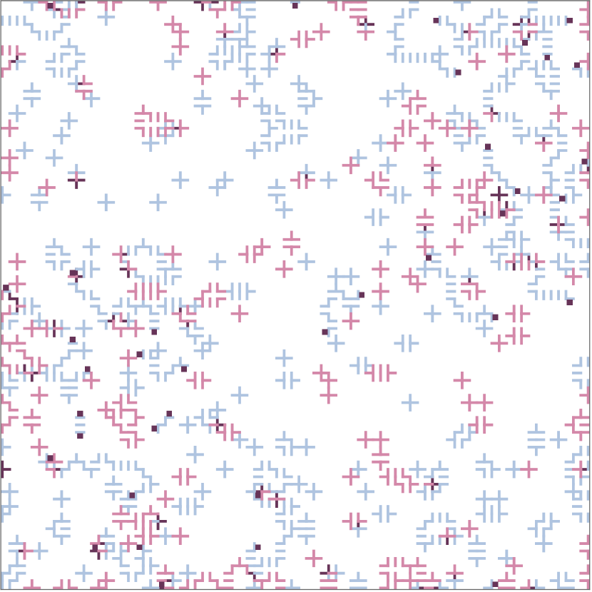
c Blue edges correspond to the support of $\hat{\sigma}$, red edges correspond to the support of $\hat{\sigma}^{\prime}$, and black squares to the support of $d\hat{\sigma}$.

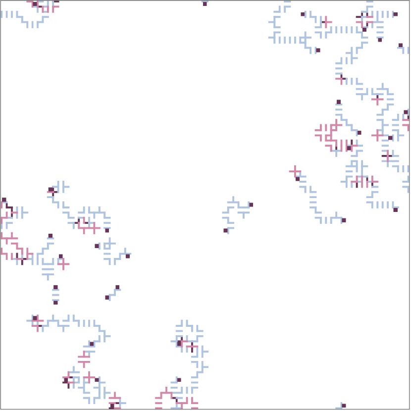
d Blue edges correspond to the support of $\hat{\sigma}|_{E_{\hat{\sigma},\hat{\sigma}^{\prime}}}$, red edges correspond to the support of $\hat{\sigma}^{\prime}|_{E_{\hat{\sigma},\hat{\sigma}^{\prime}}}$, and black squares correspond to the support of $d\hat{\sigma}$.

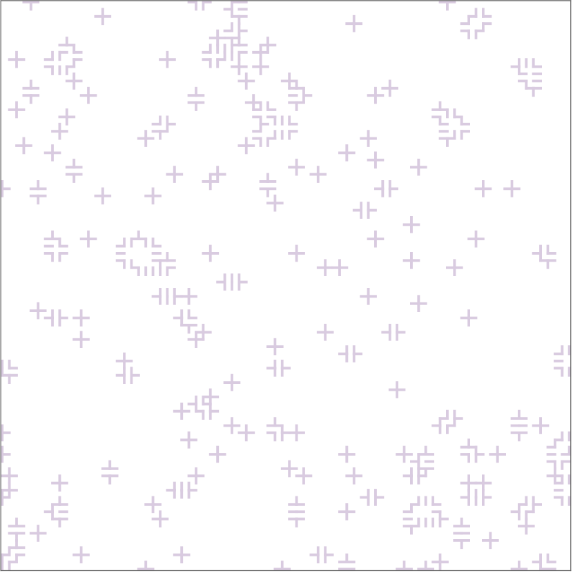
e Purple edges correspond to the support of $\hat{\sigma}|_{E_{N}\smallsetminus E_{\hat{\sigma},\hat{\sigma}^{\prime}}}$.

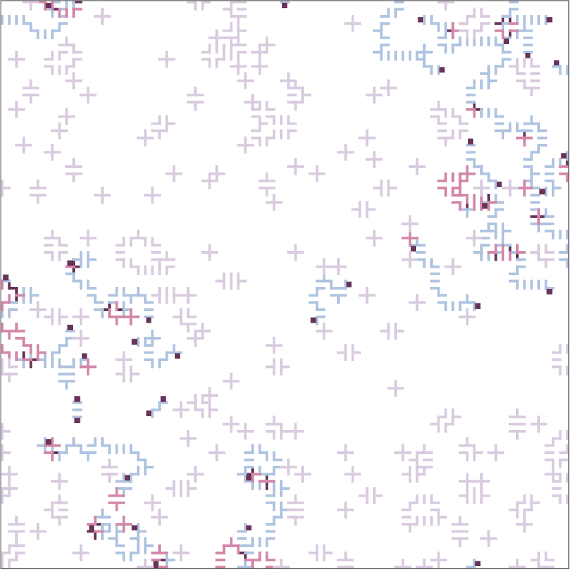
f Blue edges correspond to the support of $\hat{\sigma}|_{E_{\hat{\sigma},\hat{\sigma}^{\prime}}}$, red edges correspond to the support of $\hat{\sigma}^{\prime}|_{E_{\hat{\sigma},\hat{\sigma}^{\prime}}}$, purple edges correspond to the support of $\hat{\sigma}|_{E_{N}\smallsetminus E_{\hat{\sigma},\hat{\sigma}^{\prime}}}$, and black squares correspond to the support of $d\hat{\sigma}$.

Figure 8. Illustration of the coupling $(\sigma,\sigma^{\prime})=(\hat{\sigma},\hat{\sigma}^{\prime}|_{E_{\hat{\sigma},\hat{\sigma}^{\prime}}}+\hat{\sigma}|_{E_{N}\smallsetminus E_{\hat{\sigma},\hat{\sigma}^{\prime}}})$ defined in Definition 7.10 (simulated on a 2-dimensional lattice, with $G=\mathbb{Z}_{2}$).

Proposition 7.12.

Let $\beta,\kappa\geqslant 0$. Then $\mu_{N,(\beta,\kappa),{(\infty,\kappa})}$ is a coupling of $\mu_{N,\beta,\kappa}$ and $\mu_{N,\infty,\kappa}$.

Proof.

It is immediate from the definition that if $(\sigma,\sigma^{\prime})\sim\mu_{N,(\beta,\kappa),(\infty,\kappa)}$, then $\sigma\sim\mu_{N,\beta,\kappa}$, and it is hence sufficient to show that $\sigma^{\prime}\sim\mu_{N,\infty,\kappa}$. To this end, fix some $\sigma^{\prime}\in\Sigma_{E_{N}}^{0}$. We need to show that

$$\mu_{N,\beta,\kappa}\times\mu_{N,\infty,\kappa}\bigl{(}\bigl{\{}(\hat{\sigma},\hat{\sigma}^{\prime})\in\Sigma_{E_{N}}\times\Sigma_{E_{N}^{0}}\colon\hat{\sigma}|_{E_{N}\smallsetminus E_{\hat{\sigma},\hat{\sigma}^{\prime}}}+\hat{\sigma}^{\prime}|_{E_{\hat{\sigma},\hat{\sigma}^{\prime}}}=\sigma^{\prime}\bigr{\}}\bigr{)}=\mu_{N,\infty,\kappa}(\sigma^{\prime}),$$

or, equivalently, using (4.2) (see also (4.3)), that

$$\sum_{\hat{\sigma}\in\Sigma_{E_{N}}}\sum_{\hat{\sigma}^{\prime}\in\Sigma_{E_{N}}^{0}}\varphi_{\beta,\kappa}(\hat{\sigma})\varphi_{\beta,\kappa}(\hat{\sigma}^{\prime})\cdot\mathbb{1}\bigl{(}\hat{\sigma}|_{E_{N}\smallsetminus E_{\hat{\sigma},\hat{\sigma}^{\prime}}}+\hat{\sigma}^{\prime}|_{E_{\hat{\sigma},\hat{\sigma}^{\prime}}}=\sigma^{\prime}\bigr{)}=\varphi_{\kappa}(\sigma^{\prime})\sum_{\sigma\in\Sigma_{E_{N}}}\varphi_{\beta,\kappa}(\sigma),$$ (7.9)

where we have used that $\varphi_{\kappa}(\hat{\sigma}^{\prime})=\varphi_{\beta,\kappa}(\hat{\sigma}^{\prime})$ because $d\hat{\sigma}^{\prime}=0$. We now rewrite the left-hand side of (7.9) in order to see that this equality indeed holds.

Let $\hat{\sigma}\in\Sigma_{E_{N}}$ and $\hat{\sigma}^{\prime}\in\Sigma_{E_{N}}^{0}$. By Lemma 7.2, we have $\hat{\sigma}|_{E_{\hat{\sigma},\hat{\sigma}^{\prime}}}\leqslant\hat{\sigma}$ and $\hat{\sigma}^{\prime}|_{E_{\hat{\sigma},\hat{\sigma}^{\prime}}}\leqslant\hat{\sigma}^{\prime}$ and hence, by Lemma 4.1,

$$\varphi_{\beta,\kappa}(\hat{\sigma})=\varphi_{\beta,\kappa}\bigl{(}\hat{\sigma}|_{E_{\hat{\sigma},\hat{\sigma}^{\prime}}}\bigr{)}\varphi_{\beta,\kappa}\bigl{(}\hat{\sigma}|_{E_{N}\smallsetminus E_{\hat{\sigma},\hat{\sigma}^{\prime}}}\bigr{)}\;\;\text{and}\;\;\varphi_{\beta,\kappa}(\hat{\sigma}^{\prime})=\varphi_{\beta,\kappa}\bigl{(}\hat{\sigma}^{\prime}|_{E_{\hat{\sigma},\hat{\sigma}^{\prime}}}\bigr{)}\varphi_{\beta,\kappa}\bigl{(}\hat{\sigma}^{\prime}|_{E_{N}\smallsetminus E_{\hat{\sigma},\hat{\sigma}^{\prime}}}\bigr{)}.$$ (7.10)

Since $\hat{\sigma}^{\prime}\in\Sigma_{E_{N}}^{0}$, we have $d\hat{\sigma}^{\prime}=0$. Since $\hat{\sigma}^{\prime}|_{E_{\hat{\sigma},\hat{\sigma}^{\prime}}}\leqslant\hat{\sigma}^{\prime}$, and hence $d(\hat{\sigma}^{\prime}|_{E_{\hat{\sigma},\hat{\sigma}^{\prime}}})=0$. As $\hat{\sigma}^{\prime}|_{E_{\hat{\sigma},\hat{\sigma}^{\prime}}}$ and $\hat{\sigma}|_{E_{N}\smallsetminus E_{\hat{\sigma},\hat{\sigma}^{\prime}}}$ have disjoint supports, it follows that $\hat{\sigma}^{\prime}|_{E_{\hat{\sigma},\hat{\sigma}^{\prime}}}\leqslant\hat{\sigma}|_{E_{N}\smallsetminus E_{\hat{\sigma},\hat{\sigma}^{\prime}}}+\hat{\sigma}^{\prime}|_{E_{\hat{\sigma},\hat{\sigma}^{\prime}}}$. Thus, by Lemma 4.1,

$$\varphi_{\beta,\kappa}\bigl{(}\hat{\sigma}|_{E_{N}\smallsetminus E_{\hat{\sigma},\hat{\sigma}^{\prime}}}\bigr{)}\varphi_{\beta,\kappa}\bigl{(}\hat{\sigma}^{\prime}|_{E_{\hat{\sigma},\hat{\sigma}^{\prime}}}\bigr{)}=\varphi_{\beta,\kappa}\bigl{(}\hat{\sigma}|_{E_{N}\smallsetminus E_{\hat{\sigma},\hat{\sigma}^{\prime}}}+\hat{\sigma}^{\prime}|_{E_{\hat{\sigma},\hat{\sigma}^{\prime}}}\bigr{)}.$$ (7.11)

Similarly, by Lemma 7.2, we have $\hat{\sigma}^{\prime}|_{E_{N}\smallsetminus E_{\hat{\sigma},\hat{\sigma}^{\prime}}}\leqslant\hat{\sigma}^{\prime}$, and hence $d(\hat{\sigma}^{\prime}|_{E_{N}\smallsetminus E_{\hat{\sigma},\hat{\sigma}^{\prime}}})=0$. Since $\hat{\sigma}^{\prime}|_{E_{N}\smallsetminus E_{\hat{\sigma},\hat{\sigma}^{\prime}}}$ and $\hat{\sigma}|_{E_{\hat{\sigma},\hat{\sigma}^{\prime}}}$ have disjoint supports, it follows that $\hat{\sigma}^{\prime}|_{E_{N}\smallsetminus E_{\hat{\sigma},\hat{\sigma}^{\prime}}}\leqslant\hat{\sigma}|_{E_{\hat{\sigma},\hat{\sigma}^{\prime}}}+\hat{\sigma}^{\prime}|_{E_{N}\smallsetminus E_{\hat{\sigma},\hat{\sigma}^{\prime}}}$. Consequently, by Lemma 4.1, we have

$$\varphi_{\beta,\kappa}\bigl{(}\hat{\sigma}|_{E_{\hat{\sigma},\hat{\sigma}^{\prime}}}\bigr{)}\varphi_{\beta,\kappa}\bigl{(}\hat{\sigma}^{\prime}|_{E_{N}\smallsetminus E_{\hat{\sigma},\hat{\sigma}^{\prime}}}\bigr{)}=\varphi_{\beta,\kappa}\bigl{(}\hat{\sigma}|_{E_{\hat{\sigma},\hat{\sigma}^{\prime}}}+\hat{\sigma}^{\prime}|_{E_{N}\smallsetminus E_{\hat{\sigma},\hat{\sigma}^{\prime}}}\bigr{)}.$$ (7.12)

Using (7.10), (7.11), and (7.12), we can rewrite the left-hand side of (7.9) as follows:

$$\begin{split}&\sum_{\hat{\sigma}\in\Sigma_{E_{N}}}\sum_{\hat{\sigma}^{\prime}\in\Sigma_{E_{N}}^{0}}\varphi_{\beta,\kappa}(\hat{\sigma})\varphi_{\beta,\kappa}(\hat{\sigma}^{\prime})\cdot\mathbb{1}\bigl{(}\hat{\sigma}|_{E_{N}\smallsetminus E_{\hat{\sigma},\hat{\sigma}^{\prime}}}+\hat{\sigma}^{\prime}|_{E_{\hat{\sigma},\hat{\sigma}^{\prime}}}=\sigma^{\prime}\bigr{)}\\ &\qquad=\sum_{\hat{\sigma}\in\Sigma_{E_{N}}}\sum_{\hat{\sigma}^{\prime}\in\Sigma_{E_{N}}^{0}}\varphi_{\beta,\kappa}\bigl{(}\hat{\sigma}|_{E_{N}\smallsetminus E_{\hat{\sigma},\hat{\sigma}^{\prime}}}+\hat{\sigma}^{\prime}|_{E_{\hat{\sigma},\hat{\sigma}^{\prime}}}\bigr{)}\varphi_{\beta,\kappa}\bigl{(}\hat{\sigma}|_{E_{\hat{\sigma},\hat{\sigma}^{\prime}}}+\hat{\sigma}^{\prime}|_{E_{N}\smallsetminus E_{\hat{\sigma},\hat{\sigma}^{\prime}}}\bigr{)}\\ &\qquad\qquad\cdot\mathbb{1}\bigl{(}\hat{\sigma}|_{E_{N}\smallsetminus E_{\hat{\sigma},\hat{\sigma}^{\prime}}}+\hat{\sigma}^{\prime}|_{E_{\hat{\sigma},\hat{\sigma}^{\prime}}}=\sigma^{\prime}\bigr{)}\\ &\qquad=\varphi_{\beta,\kappa}\bigl{(}\sigma^{\prime}\bigr{)}\sum_{\hat{\sigma}\in\Sigma_{E_{N}}}\sum_{\hat{\sigma}^{\prime}\in\Sigma_{E_{N}}^{0}}\varphi_{\beta,\kappa}\bigl{(}\hat{\sigma}|_{E_{\hat{\sigma},\hat{\sigma}^{\prime}}}+\hat{\sigma}^{\prime}|_{E_{N}\smallsetminus E_{\hat{\sigma},\hat{\sigma}^{\prime}}}\bigr{)}\cdot\mathbb{1}\bigl{(}\hat{\sigma}|_{E_{N}\smallsetminus E_{\hat{\sigma},\hat{\sigma}^{\prime}}}+\hat{\sigma}^{\prime}|_{E_{\hat{\sigma},\hat{\sigma}^{\prime}}}=\sigma^{\prime}\bigr{)}\\ &\qquad=\varphi_{\beta,\kappa}\bigl{(}\sigma^{\prime}\bigr{)}\sum_{\sigma\in\Sigma_{E_{N}}}\varphi_{\beta,\kappa}(\sigma)\sum_{\hat{\sigma}\in\Sigma_{E_{N}}}\sum_{\hat{\sigma}^{\prime}\in\Sigma_{E_{N}}^{0}}\mathbb{1}\bigl{(}\hat{\sigma}|_{E_{\hat{\sigma},\hat{\sigma}^{\prime}}}+\hat{\sigma}^{\prime}|_{E_{N}\smallsetminus E_{\hat{\sigma},\hat{\sigma}^{\prime}}}=\sigma\bigr{)}\\ &\qquad\qquad\cdot\mathbb{1}\bigl{(}\hat{\sigma}|_{E_{N}\smallsetminus E_{\hat{\sigma},\hat{\sigma}^{\prime}}}+\hat{\sigma}^{\prime}|_{E_{\hat{\sigma},\hat{\sigma}^{\prime}}}=\sigma^{\prime}\bigr{)}.\end{split}$$ (7.13)

Now note that, by Lemma 7.4, we have $E_{\hat{\sigma},\hat{\sigma}^{\prime}}=E_{\sigma,\sigma^{\prime}}$. Consequently, for any $\sigma\in\Sigma_{E_{N}}$, we have

$$\begin{split}&\sum_{\hat{\sigma}\in\Sigma_{E_{N}}}\sum_{\hat{\sigma}^{\prime}\in\Sigma_{E_{N}}^{0}}\mathbb{1}\bigl{(}\hat{\sigma}|_{E_{\hat{\sigma},\hat{\sigma}^{\prime}}}+\hat{\sigma}^{\prime}|_{E_{N}\smallsetminus E_{\hat{\sigma},\hat{\sigma}^{\prime}}}=\sigma\bigr{)}\cdot\mathbb{1}\bigl{(}\hat{\sigma}|_{E_{N}\smallsetminus E_{\hat{\sigma},\hat{\sigma}^{\prime}}}+\hat{\sigma}^{\prime}|_{E_{\hat{\sigma},\hat{\sigma}^{\prime}}}=\sigma^{\prime}\bigr{)}\\ &\qquad=\sum_{\hat{\sigma}\in\Sigma_{E_{N}}}\sum_{\hat{\sigma}^{\prime}\in\Sigma_{E_{N}}^{0}}\mathbb{1}\bigl{(}\hat{\sigma}|_{E_{\sigma,\sigma^{\prime}}}+\hat{\sigma}^{\prime}|_{E_{N}\smallsetminus E_{\sigma,\sigma^{\prime}}}=\sigma\bigr{)}\cdot\mathbb{1}\bigl{(}\hat{\sigma}|_{E_{N}\smallsetminus E_{\sigma,\sigma^{\prime}}}+\hat{\sigma}^{\prime}|_{E_{\sigma,\sigma^{\prime}}}=\sigma^{\prime}\bigr{)}\\ &\qquad=\sum_{\hat{\sigma}\in\Sigma_{E_{N}}}\sum_{\hat{\sigma}^{\prime}\in\Sigma_{E_{N}}^{0}}\mathbb{1}\bigl{(}\hat{\sigma}=\sigma|_{E_{\sigma,\sigma^{\prime}}}+\sigma^{\prime}|_{E_{N}\smallsetminus E_{\sigma,\sigma^{\prime}}}\bigr{)}\cdot\mathbb{1}\bigl{(}\hat{\sigma}^{\prime}=\sigma|_{E_{N}\smallsetminus E_{\sigma,\sigma^{\prime}}}+\sigma^{\prime}|_{E_{\sigma,\sigma^{\prime}}}\bigr{)}.\end{split}$$ (7.14)

Since $\sigma\in\Sigma_{E_{N}}$ and $\sigma^{\prime}\in\Sigma_{E_{N}}^{0}$, we can apply Lemma 7.3 to obtain $\sigma^{\prime}|_{E_{\sigma,\sigma^{\prime}}}+\sigma_{E_{N}\smallsetminus E_{\sigma,\sigma^{\prime}}}\in\Sigma_{E_{N}}^{0}$. From this it follows that the double sum on the right-hand side of (7.14) is equal to $1$. Inserting this into the last line of (7.13) and using that $\varphi_{\beta,\kappa}(\sigma^{\prime})=\varphi_{\kappa}(\sigma^{\prime})$, we obtain (7.9) as desired. This concludes the proof. ∎

In what follows, we collect a few useful properties of the coupling introduced in Definition 7.10 for easy reference in later sections.

Lemma 7.13.

Let $\beta,\kappa\geqslant 0$ and assume that $\mu_{N,(\beta,\kappa),(\infty,\kappa)}(\sigma,\sigma^{\prime})\neq 0$. Then $\sigma_{e}=\sigma^{\prime}_{e}$ for all $e\in E_{N}\smallsetminus E_{\sigma,\sigma^{\prime}}$.

Proof.

Since $\mu_{N,(\beta,\kappa),(\infty,\kappa)}(\sigma,\sigma^{\prime})\neq 0$, by definition, there is $(\hat{\sigma},\hat{\sigma}^{\prime})\in E_{N}\times E_{N}^{0}$ such that $\sigma=\hat{\sigma}$ and $\sigma^{\prime}=\hat{\sigma}^{\prime}|_{E_{\hat{\sigma},\hat{\sigma}^{\prime}}}+\hat{\sigma}|_{E_{N}\smallsetminus E_{\hat{\sigma},\hat{\sigma}^{\prime}}}$. Using Lemma 7.4, we immediately obtain the desired conclusion. ∎

Lemma 7.14.

Let $(\sigma,\sigma^{\prime})\in\Sigma_{E_{N}}\times\Sigma_{E_{N}}^{0}$. Then $e\in E_{\sigma,\sigma^{\prime}}$ if and only if $d(\sigma|_{\mathcal{C}_{\mathcal{G}(\sigma,\sigma^{\prime})}(e)})\neq 0$.

Proof.

Let $\mathcal{G}\coloneqq\mathcal{G}(\sigma,\sigma^{\prime})$. Suppose first that $e\in E_{\sigma,\sigma^{\prime}}$. By the definition of $\mathcal{C}_{\mathcal{G}}(e)$, there exists an edge $e_{1}\in\mathcal{C}_{\mathcal{G}}(e)$ such that $e_{1}\in\operatorname{supp}\sigma\cap\partial\operatorname{supp}d\sigma$. We infer that there exists a plaquette $p_{1}\in\hat{\partial}e_{1}$ such that $(d\sigma)_{p_{1}}\neq 0$. Since $e_{1}\in\mathcal{C}_{\mathcal{G}}(e)$, all edges in $\operatorname{supp}\sigma\cap\partial p_{1}$ are contained in $\mathcal{C}_{\mathcal{G}}(e)$, and so $(d(\sigma|_{\mathcal{C}_{\mathcal{G}}(e)}))_{p_{1}}=(d\sigma)_{p_{1}}\neq 0$.

Conversely, suppose that there is a plaquette $p_{1}\in P_{N}$ such that $(d(\sigma|_{\mathcal{C}_{\mathcal{G}}(e)}))_{p_{1}}\neq 0$. Then there exists an edge $e_{1}\in\partial p_{1}$ with $\sigma_{e_{1}}\neq 0$ and $e_{1}\in\mathcal{C}_{\mathcal{G}}(e)$. It follows that $\operatorname{supp}\sigma\cap\partial p_{1}\subseteq\mathcal{C}_{\mathcal{G}}(e)$, and so $(d\sigma)_{p_{1}}=(d(\sigma|_{\mathcal{C}_{\mathcal{G}}(e)}))_{p_{1}}\neq 0$; in particular $e_{1}\in\partial p_{1}\subseteq\partial\operatorname{supp}d\sigma$. Consequently, $e_{1}$ must belong to the set $\operatorname{supp}\sigma\cap\partial\operatorname{supp}d\sigma$. In particular, $e_{1}\in E_{\sigma,\sigma^{\prime}}$ and thus $e\in\mathcal{C}_{\mathcal{G}}(e_{1})\subseteq E_{\sigma,\sigma^{\prime}}$. ∎

For $e\in E_{N}$, we let $\operatorname{dist}(e,B_{N}^{c})$ denote the smallest Euclidean distance between the midpoint of $e$ and the midpoints of the edges on the boundary of $B_{N}$. For $E\subseteq E_{N}$, we let $\operatorname{dist}(E,B_{N}^{c})\coloneqq\min_{e\in E}\operatorname{dist}(e,B_{N}^{c})$.

In the remainder of this section, we provide proofs of the following three propositions, which will all be used later in the proofs of our main results. Heuristically, these propositions all give upper bounds for local events related to the coupling. For all of these local events, the main proof idea is to combine Proposition 5.1 with an enumeration of all spin configurations which belong to the given local event.

Proposition 7.15.

Let $\beta,\kappa\geqslant 0$ be such that [A3] holds, and let $e\in E_{N}$ be such that $\partial\hat{\partial}\partial\hat{\partial}e\subseteq E_{N}$. Then

$$\begin{split}&\mu_{N,(\beta,\kappa),(\infty,\kappa)}\bigl{(}\bigl{\{}(\sigma,\sigma^{\prime})\in\Sigma_{E_{N}}\times\Sigma_{E_{N}}^{0}\colon e\in E_{\sigma,\sigma^{\prime}}\text{ and }\sigma_{e}^{\prime}\neq 0\bigr{\}}\bigr{)}\\ &\qquad\leqslant C_{c,1}\alpha_{0}(\kappa)^{9}\alpha_{1}(\beta)^{6}+C_{c,1}^{\prime}\Bigl{(}18^{2}\bigl{(}2+\alpha_{0}(\kappa)\bigr{)}\alpha_{0}(\kappa)\Bigr{)}^{\operatorname{dist}(e,B_{N}^{c})},\end{split}$$ (7.15)

where

$$C_{c,1}\coloneqq 18^{13}\cdot\frac{\sum_{j=1}^{8}\binom{8}{j}2^{8-j}\alpha_{0}(\kappa)^{j-1}+2^{8}18^{2}\bigl{(}2+\alpha_{0}(\kappa)\bigr{)}}{1-18^{2}\bigl{(}2\alpha_{0}(\kappa)+\alpha_{0}(\kappa)^{2}\bigr{)}}$$ (7.16)

and

$$C_{c,1}^{\prime}\coloneqq\frac{1}{18^{3}\big{(}1-18^{2}(2+\alpha_{0}(\kappa))\alpha_{0}(\kappa)\big{)}}.$$ (7.17)

Remark 7.16.

With very small modifications to the proof of Proposition 7.15, one can prove a result which considers the same event as in (7.15) but without the condition $\sigma_{e}^{\prime}\neq 0.$ This shows that far from the boundary of $B_{N}$, the probability that the coupled configurations $\sigma$ and $\sigma^{\prime}$ disagree on a given edge $e\in E_{N}$ is of order $\alpha_{2}(\beta,\kappa)^{6}.$

Proposition 7.17.

Let $\beta,\kappa\geqslant 0$ be such that [A3] holds. If $e\in E_{N}$ satisfies $\partial\hat{\partial}\partial\hat{\partial}e\subseteq E_{N}$, then

$$\begin{split}&\mu_{N,(\beta,\kappa),(\infty,\kappa)}\bigl{(}\bigl{\{}(\sigma,\sigma^{\prime})\in\Sigma_{E_{N}}\times\Sigma_{E_{N}}^{0}\colon e\in\partial\hat{\partial}E_{\sigma,\sigma^{\prime}}\text{ and }\sigma\in\mathcal{E}\}\bigr{)}\\ &\qquad\leqslant C_{c,2}\alpha_{1}(\beta)^{6}\alpha_{0}(\kappa)^{6}\max\bigl{(}\alpha_{0}(\kappa),\alpha_{1}(\beta)^{6}\bigr{)}+C_{c,2}^{\prime}\Bigl{(}18^{2}\bigl{(}2+\alpha_{0}(\kappa)\bigr{)}\alpha_{0}(\kappa)\Bigr{)}^{\operatorname{dist}(e,B_{N}^{c})},\end{split}$$ (7.18)

where the event $\mathcal{E}$ is defined by

$$\mathcal{E}\coloneqq\bigl{\{}\sigma\in\Sigma_{E_{N}}\colon\exists g\in G\smallsetminus\{0\}\text{ such that }\sigma_{e}-(d\sigma)_{p}=g\text{ for all }p\in\hat{\partial}e\bigr{\}},$$

$$C_{c,2}\coloneqq\frac{2\cdot 18^{11}(18^{2}+1)\bigl{(}1+2\alpha_{0}(\kappa)+\alpha_{0}(\kappa)^{2}\bigr{)}\bigl{(}2+\alpha_{0}(\kappa)\bigr{)}^{7}}{1-18^{2}(2\alpha_{0}(\kappa)+\alpha_{0}(\kappa)^{2})},$$ (7.19)

and

$$C_{c,2}^{\prime}\coloneqq\frac{1+2\alpha_{0}(\kappa)+\alpha_{0}(\kappa)^{2}}{18^{3}(1-18^{2}\bigl{(}2+\alpha_{0}(\kappa)\bigr{)}\alpha_{0}(\kappa))}\cdot\biggl{(}1+\frac{1}{\bigl{(}2+\alpha_{0}(\kappa)\bigr{)}\alpha_{0}(\kappa)}\biggr{)}.$$ (7.20)

Remark 7.18.

We note that if $N\to\infty$ while $e$, $\beta$, and $\kappa$ remain fixed, then the terms involving $\operatorname{dist}(e,B_{N}^{c})$ on the right-hand sides of (7.15) and (7.18) tend to zero.

Proposition 7.19.

Let $\beta,\kappa\geqslant 0$ be such that [A3] holds, and let $e\in E_{N}^{+}$ be such that $\partial\hat{\partial}\partial\hat{\partial}e\in E_{N}$. Then

$$\mu_{N,\infty,\kappa}\bigl{(}\{\sigma^{\prime}\in\Sigma_{E_{N}}^{0}\colon\sigma_{e}^{\prime}\neq 0\}\bigr{)}\leqslant C_{I}\alpha_{0}(\kappa)^{8},$$ (7.21)

where

$$C_{I}\coloneqq\frac{18^{13}}{1-18^{2}\alpha_{0}(\kappa)},$$ (7.22)

Before we provide proofs of the three propositions above, we introduce some additional notation and prove two useful lemmas.

If $\mathcal{G}$ is a finite graph, we say that a walk $W=(v_{1},\ldots,v_{m})$ in $\mathcal{G}$ is a spanning walk of $\mathcal{G}$ if it passes through each vertex of $G$ at least once. We say that a walk $W=(v_{1},\ldots,v_{m})$ has length $m-1$.

Lemma 7.20.

Let $\mathcal{G}$ be a connected graph on $m\geqslant 2$ vertices. Then there is a walk $W$ in $\mathcal{G}$ of length $2m-3$ which passes through each vertex at least once.

Proof.

Since $\mathcal{G}$ is connected, $\mathcal{G}$ has a spanning tree. Any such spanning tree must contain exactly $m-1$ edges. Using this tree, one can find a spanning walk which uses each edge in the tree exactly twice. This walk must have length $2(m-1)=2m-2$. Removing the last edge in this walk, we obtain a walk with the desired properties. This concludes the proof. ∎

Fix some $g\in G\smallsetminus\{0\}$ and define $\sigma\in\Sigma_{E_{N}}$ by letting $\sigma_{e}=g$ for all $e\in E_{N}^{+}$. Let $\bar{\mathcal{G}}\coloneqq\mathcal{G}(\sigma,0)$ and note that $\bar{\mathcal{G}}$ does not depend on the choice of $g$. Note also that if $\sigma^{(0)},\sigma^{(1)}\in\Sigma_{E_{N}}$, then $\mathcal{G}(\sigma^{(0)},\sigma^{(1)})$ is a subgraph of $\bar{\mathcal{G}}$.

Lemma 7.21.

Let $e\in E_{N}$ and let $m\geqslant 1$. Then there are at most $18^{m}$ walks of length $m$ in $\bar{\mathcal{G}}$ containing only edges in $E_{N}^{+}$, and starting at $e$.

Proof.

For each $e\in E_{N}$, we have $|(\partial\hat{\partial}e)\smallsetminus\{e\}|=6\cdot 3=18$. Moreover,

$$\bigl{(}(\partial\hat{\partial}e)\smallsetminus\{e\}\bigr{)}\cap\Bigl{(}-\bigl{(}(\partial\hat{\partial}e)\smallsetminus\{e\}\bigr{)}\Bigr{)}=\emptyset,$$

and hence

$$\Bigl{|}\bigl{(}(\partial\hat{\partial}e)\smallsetminus\{e\}\bigr{)}^{+}\cup\Bigl{(}-\bigl{(}(\partial\hat{\partial}e)\smallsetminus\{e\}\bigr{)}\Bigr{)}^{+}\Bigr{|}=|(\partial\hat{\partial}e)\smallsetminus\{e\}|=18,$$

from which the desired conclusion follows. ∎

Proof of Proposition 7.15.

By using first the definition of $\mu_{N,(\beta,\kappa),(\infty,\kappa)}$ and then Lemma 7.4, we see that

$$\begin{split}&\mu_{N,(\beta,\kappa),(\infty,\kappa)}\bigl{(}\big{\{}(\sigma,\sigma^{\prime})\in\Sigma_{E_{N}}\times\Sigma_{E_{N}}^{0}\colon e\in E_{\sigma,\sigma^{\prime}}\text{ and }\sigma_{e}^{\prime}\neq 0\big{\}}\bigr{)}\\ &\qquad=\mu_{N,\beta,\kappa}\times\mu_{N,\infty,\kappa}\bigl{(}\big{\{}(\hat{\sigma},\hat{\sigma}^{\prime})\in\Sigma_{E_{N}}\times\Sigma_{E_{N}}^{0}\colon e\in E_{\hat{\sigma},\hat{\sigma}^{\prime}|_{E_{\hat{\sigma},\hat{\sigma}^{\prime}}}+\hat{\sigma}|_{E_{N}\smallsetminus E_{\hat{\sigma},\hat{\sigma}^{\prime}}}}\text{ and }\hat{\sigma}_{e}^{\prime}\neq 0\big{\}}\bigr{)}\\ &\qquad=\mu_{N,\beta,\kappa}\times\mu_{N,\infty,\kappa}\bigl{(}\big{\{}(\hat{\sigma},\hat{\sigma}^{\prime})\in\Sigma_{E_{N}}\times\Sigma_{E_{N}}^{0}\colon e\in E_{\hat{\sigma},\hat{\sigma}^{\prime}}\text{ and }\hat{\sigma}_{e}^{\prime}\neq 0\big{\}}\bigr{)}.\end{split}$$

By Lemma 7.14, for any $(\hat{\sigma},\hat{\sigma}^{\prime})\in\Sigma_{E_{N}}\times\Sigma_{E_{N}}^{0}$, we have

$$e\in E_{\hat{\sigma},\hat{\sigma}^{\prime}}\Leftrightarrow d(\hat{\sigma}|_{\mathcal{C}_{\mathcal{G}(\hat{\sigma},\hat{\sigma}^{\prime})}(e)})\neq 0.$$

Consequently, the desired conclusion will follow if we can show that

$$\begin{split}&\mu_{N,\beta,\kappa}\times\mu_{N,\infty,\kappa}\bigl{(}\big{\{}(\hat{\sigma},\hat{\sigma}^{\prime})\in\Sigma_{E_{N}}\times\Sigma_{E_{N}}^{0}\colon d(\hat{\sigma}|_{\mathcal{C}_{\mathcal{G}(\hat{\sigma},\hat{\sigma}^{\prime})}(e)})\neq 0\text{ and }\hat{\sigma}_{e}^{\prime}\neq 0\big{\}}\bigr{)}\\ &\qquad\leqslant C_{c,1}\alpha_{0}(\kappa)^{9}\alpha_{1}(\beta)^{6}+C_{c,1}^{\prime}\Bigl{(}18^{2}\bigl{(}2+\alpha_{0}(\kappa)\bigr{)}\alpha_{0}(\kappa)\Bigr{)}^{\operatorname{dist}(e,B_{N}^{c})}.\end{split}$$ (7.23)

If $(\hat{\sigma},\hat{\sigma}^{\prime})\in\Sigma_{E_{N}}\times\Sigma_{E_{N}}^{0}$ and $d(\hat{\sigma}|_{\mathcal{C}_{\mathcal{G}(\hat{\sigma},\hat{\sigma}^{\prime})}(e)})\neq 0$, the set $\mathcal{C}_{\mathcal{G}(\hat{\sigma},\hat{\sigma}^{\prime})}(e)$ must be non-empty. Since $\mathcal{C}_{\mathcal{G}(\hat{\sigma},\hat{\sigma}^{\prime})}(e)$ is symmetric, the cardinality $|\mathcal{C}_{\mathcal{G}(\hat{\sigma},\hat{\sigma}^{\prime})}(e)|\geqslant 1$ must be even. From these observations, we obtain

$$\begin{split}&\mu_{N,\beta,\kappa}\times\mu_{N,\infty,\kappa}\bigl{(}\big{\{}(\hat{\sigma},\hat{\sigma}^{\prime})\in\Sigma_{E_{N}}\times\Sigma_{E_{N}}^{0}\colon d(\hat{\sigma}|_{\mathcal{C}_{\mathcal{G}(\hat{\sigma},\hat{\sigma}^{\prime})}(e)})\neq 0\text{ and }\hat{\sigma}_{e}^{\prime}\neq 0\big{\}}\bigr{)}\\ &=\sum_{m=1}^{\infty}\mu_{N,\beta,\kappa}\times\mu_{N,\infty,\kappa}\bigl{(}\big{\{}(\hat{\sigma},\hat{\sigma}^{\prime})\in\Sigma_{E_{N}}\times\Sigma_{E_{N}}^{0}\colon d(\hat{\sigma}|_{\mathcal{C}_{\mathcal{G}(\hat{\sigma},\hat{\sigma}^{\prime})}(e)})\neq 0,\,\hat{\sigma}_{e}^{\prime}\neq 0,\,|\mathcal{C}_{\mathcal{G}(\hat{\sigma},\hat{\sigma}^{\prime})}(e)|=2m\big{\}}\bigr{)}.\end{split}$$

Next, for $k\geqslant 1$, let $T_{e,k}$ be the set of all walks in $\bar{\mathcal{G}}$ which start at $e$, have length $2k-3$, contain only edges in $E_{N}^{+}$, and visit exactly $k$ vertices in $\bar{\mathcal{G}}$. Given $(\hat{\sigma},\hat{\sigma}^{\prime})\in\Sigma_{E_{N}}\times\Sigma_{E_{N}}^{0}$, and $\mathcal{G}=\mathcal{G}(\hat{\sigma},\hat{\sigma}^{\prime})$, let $\mathcal{G}|_{(\mathcal{C}_{\mathcal{G}}(e))^{+}}$ denote the graph $\mathcal{G}$ restricted to the set $(\mathcal{C}_{\mathcal{G}}(e))^{+}$, and let $\mathcal{W}_{\hat{\sigma},\hat{\sigma}^{\prime},e}$ be the set of all spanning walks of $\mathcal{G}|_{(\mathcal{C}_{\mathcal{G}}(e))^{+}}$ which have length $2|(\mathcal{C}_{\mathcal{G}}(e))^{+}|-3$ and start at $e$. By Lemma 7.20, the set $\mathcal{W}_{\hat{\sigma},\hat{\sigma}^{\prime},e}$ is non-empty. Moreover, since any walk on $\mathcal{G}$ is a walk on $\bar{\mathcal{G}}$, we have $\mathcal{W}_{\hat{\sigma},\hat{\sigma}^{\prime},e}\subseteq T_{e,|(\mathcal{C}_{\mathcal{G}}(e))^{+}|}$. Hence

$$\sum_{m=1}^{\infty}\mu_{N,\beta,\kappa}\times\mu_{N,\infty,\kappa}\bigl{(}\big{\{}(\hat{\sigma},\hat{\sigma}^{\prime})\in\Sigma_{E_{N}}\times\Sigma_{E_{N}}^{0}\colon d(\hat{\sigma}|_{\mathcal{C}_{\mathcal{G}(\hat{\sigma},\hat{\sigma}^{\prime})}(e)})\neq 0,\,\hat{\sigma}_{e}^{\prime}\neq 0,\,|\mathcal{C}_{\mathcal{G}(\hat{\sigma},\hat{\sigma}^{\prime})}(e)|=2m\big{\}}\bigr{)}$$

$$\qquad\leqslant\sum_{m=1}^{\infty}\sum_{W\in T_{e,m}}\mu_{N,\beta,\kappa}\times\mu_{N,\infty,\kappa}\bigl{(}\big{\{}(\hat{\sigma},\hat{\sigma}^{\prime})\in\Sigma_{E_{N}}\times\Sigma_{E_{N}}^{0}\colon d(\hat{\sigma}|_{\mathcal{C}_{\mathcal{G}(\hat{\sigma},\hat{\sigma}^{\prime})}(e)})\neq 0,\,\hat{\sigma}_{e}^{\prime}\neq 0,\,$$ (7.24)

$$\hskip 190.00029pt|\mathcal{C}_{\mathcal{G}(\hat{\sigma},\hat{\sigma}^{\prime})}(e)|=2m\text{ and }W\in\mathcal{W}_{\hat{\sigma},\hat{\sigma}^{\prime},e}\big{\}}\bigr{)}.$$

Now assume that $W\in T_{e,m}$ for some $m\geqslant 1$. Let $\operatorname{supp}W$ be the set of edges in $E_{N}^{+}$ traversed by $W$. Then $\bigl{(}\mathcal{C}_{\mathcal{G}(\hat{\sigma},\hat{\sigma}^{\prime})}(e)\bigr{)}^{+}=\operatorname{supp}W$ whenever $|\mathcal{C}_{\mathcal{G}(\hat{\sigma},\hat{\sigma}^{\prime})}(e)|=2m$ and $W\in\mathcal{W}_{\hat{\sigma},\hat{\sigma}^{\prime},e}$. Consequently, the expression on the right-hand side of (7.24) is bounded from above by

$$\begin{split}&\sum_{m=1}^{\infty}\sum_{W\in T_{e,m}}\mu_{N,\beta,\kappa}\times\mu_{N,\infty,\kappa}\bigl{(}\{(\hat{\sigma},\hat{\sigma}^{\prime})\in\Sigma_{E_{N}}\times\Sigma_{E_{N}}^{0}\colon d(\hat{\sigma}|_{\mathcal{C}_{\mathcal{G}(\hat{\sigma},\hat{\sigma}^{\prime})}(e)})\neq 0,\,\hat{\sigma}_{e}^{\prime}\neq 0,\\[-4.30554pt] &\hskip 240.00037pt\bigl{(}\mathcal{C}_{\mathcal{G}(\hat{\sigma},\hat{\sigma}^{\prime})}(e)\bigr{)}^{+}=\operatorname{supp}W\}\bigr{)}.\end{split}$$ (7.25)

Given $(\hat{\sigma},\hat{\sigma}^{\prime})\in\Sigma_{E_{N}}\times\Sigma_{E_{N}}^{0}$, if we let $\sigma\coloneqq\hat{\sigma}|_{\mathcal{C}_{\mathcal{G}(\hat{\sigma},\hat{\sigma}^{\prime})}(e)}$ and $\sigma^{\prime}\coloneqq\hat{\sigma}^{\prime}|_{\mathcal{C}_{\mathcal{G}(\hat{\sigma},\hat{\sigma}^{\prime})}(e)}$, then the following statements hold.

1. By Lemma 7.2, $\sigma^{\prime}\leqslant\hat{\sigma}^{\prime}$. Since $\hat{\sigma}^{\prime}\in\Sigma_{E_{N}}^{0}$, it follows that $\sigma^{\prime}\in\Sigma_{E_{N}}^{0}$.

2. If $d(\hat{\sigma}|_{\mathcal{C}_{\mathcal{G}(\hat{\sigma},\hat{\sigma}^{\prime})}(e)})\neq 0$, then $d\sigma\neq 0.$

3. If $d(\hat{\sigma}|_{\mathcal{C}_{\mathcal{G}(\hat{\sigma},\hat{\sigma}^{\prime})}(e)})\neq 0$, then $e\in\operatorname{supp}\hat{\sigma}\cup\operatorname{supp}\hat{\sigma}^{\prime}$ and thus $(\mathcal{C}_{\mathcal{G}(\hat{\sigma},\hat{\sigma}^{\prime})}(e))^{+}=(\operatorname{supp}\sigma\cup\operatorname{supp}\sigma^{\prime})^{+}$. Hence, if $d(\hat{\sigma}|_{\mathcal{C}_{\mathcal{G}(\hat{\sigma},\hat{\sigma}^{\prime})}(e)})\neq 0$, then $(\mathcal{C}_{\mathcal{G}(\hat{\sigma},\hat{\sigma}^{\prime})}(e))^{+}=\operatorname{supp}W$ if and only if $(\operatorname{supp}\sigma\cup\operatorname{supp}\sigma^{\prime})^{+}=\operatorname{supp}W.$

4. $\hat{\sigma}_{e}^{\prime}=\sigma_{e}^{\prime}.$

As a consequence, the expression in (7.25) is bounded from above by

$$\begin{split}&\sum_{m=1}^{\infty}\sum_{W\in T_{e,m}}\sum_{\begin{subarray}{c}\sigma\in\Sigma_{E_{N}},\,\sigma^{\prime}\in\Sigma_{E_{N}}^{0}\colon\\ \begin{subarray}{c}(\operatorname{supp}\sigma\cup\operatorname{supp}\sigma^{\prime})^{+}=\operatorname{supp}W,\\ d\sigma\neq 0,\,\sigma^{\prime}_{e}\neq 0\end{subarray}\end{subarray}}\mu_{N,\beta,\kappa}\times\mu_{N,\infty,\kappa}\bigl{(}\{(\hat{\sigma},\hat{\sigma}^{\prime})\in\Sigma_{E_{N}}\times\Sigma_{E_{N}}^{0}\colon\\[-30.1388pt] &\hskip 220.00034pt\hat{\sigma}|_{\mathcal{C}_{\mathcal{G}(\hat{\sigma},\hat{\sigma}^{\prime})}(e)}=\sigma,\text{ and }\hat{\sigma}^{\prime}|_{\mathcal{C}_{\mathcal{G}(\hat{\sigma},\hat{\sigma}^{\prime}}(e)}=\sigma^{\prime}\}\bigr{)}\\ &\mbox{}\end{split}$$

For any $m$, $W$, $\sigma$, and $\sigma^{\prime}$ as in the sum above, by Lemma 7.2, we have

$$\begin{split}&\mu_{N,\beta,\kappa}\times\mu_{N,\infty,\kappa}\bigl{(}\{(\hat{\sigma},\hat{\sigma}^{\prime})\in\Sigma_{E_{N}}\times\Sigma_{E_{N}}^{0}\colon\hat{\sigma}|_{\mathcal{C}_{\mathcal{G}(\hat{\sigma},\hat{\sigma}^{\prime})}(e)}=\sigma\text{ and }\hat{\sigma}^{\prime}|_{\mathcal{C}_{\mathcal{G}(\hat{\sigma},\hat{\sigma}^{\prime}}(e)}=\sigma^{\prime}\}\bigr{)}\\ &\qquad\leqslant\mu_{N,\beta,\kappa}\times\mu_{N,\infty,\kappa}\bigl{(}\{(\hat{\sigma},\hat{\sigma}^{\prime})\in\Sigma_{E_{N}}\times\Sigma_{E_{N}}^{0}\colon\sigma\leqslant\hat{\sigma}\text{ and }\sigma^{\prime}\leqslant\hat{\sigma}^{\prime}\}\bigr{)}\\ &\qquad=\mu_{N,\beta,\kappa}\bigl{(}\{\hat{\sigma}\in\Sigma_{E_{N}}\colon\sigma\leqslant\hat{\sigma}\}\bigr{)}\mu_{N,\infty,\kappa}\bigl{(}\{\hat{\sigma}^{\prime}\in\Sigma_{E_{N}}^{0}\colon\sigma^{\prime}\leqslant\hat{\sigma}^{\prime}\}\bigr{)}\leqslant\varphi_{\beta,\kappa}(\sigma)\varphi_{\infty,\kappa}(\sigma^{\prime}),\end{split}$$

where the last inequality follows by applying Proposition 5.1 twice. Taken together, the above equations show that

$$\begin{split}&\mu_{N,\beta,\kappa}\times\mu_{N,\infty,\kappa}\bigl{(}\{(\hat{\sigma},\hat{\sigma}^{\prime})\in\Sigma_{E_{N}}\times\Sigma_{E_{N}}^{0}\colon e\in E_{\hat{\sigma},\hat{\sigma}^{\prime}},\,\hat{\sigma}^{\prime}_{e}\neq 0\}\bigr{)}\leqslant\sum_{m=1}^{\infty}\sum_{W\in T_{e,m}}J_{\beta,\kappa}(W),\end{split}$$ (7.26)

where

$$J_{\beta,\kappa}(W)\coloneqq\sum_{\begin{subarray}{c}\sigma\in\Sigma_{E_{N}},\,\sigma^{\prime}\in\Sigma_{E_{N}}^{0}\colon\\ \begin{subarray}{c}(\operatorname{supp}\sigma\cup\operatorname{supp}\sigma^{\prime})^{+}=\operatorname{supp}W,\\ d\sigma\neq 0,\,\sigma^{\prime}_{e}\neq 0\end{subarray}\end{subarray}}\varphi_{\beta,\kappa}(\sigma)\,\varphi_{\infty,\kappa}(\sigma^{\prime}).$$

Fix some $m\geqslant 1$ and $W\in T_{e,m}$. Then

$$\begin{split}&J_{\beta,\kappa}(W)=\sum_{\begin{subarray}{c}\sigma\in\Sigma_{E_{N}},\,\sigma^{\prime}\in\Sigma_{E_{N}}^{0}\colon\\ \begin{subarray}{c}(\operatorname{supp}\sigma\cup\operatorname{supp}\sigma^{\prime})^{+}=\operatorname{supp}W,\\ d\sigma\neq 0,\,\sigma^{\prime}_{e}\neq 0\end{subarray}\end{subarray}}\prod_{e^{\prime}\in E_{N}}\varphi_{\kappa}(\sigma_{e^{\prime}})\prod_{p\in P_{N}}\varphi_{\beta}\bigl{(}(d\sigma)_{p}\bigr{)}\prod_{e^{\prime\prime}\in E_{N}}\varphi_{\kappa}(\sigma_{e^{\prime\prime}}^{\prime})\\ &\qquad=\sum_{\begin{subarray}{c}\sigma\in\Sigma_{E_{N}},\,\sigma^{\prime}\in\Sigma_{E_{N}}^{0}\colon\\ \begin{subarray}{c}(\operatorname{supp}\sigma\cup\operatorname{supp}\sigma^{\prime})^{+}=\operatorname{supp}W,\\ d\sigma\neq 0,\,\sigma^{\prime}_{e}\neq 0\end{subarray}\end{subarray}}\prod_{e^{\prime}\in E_{N}^{+}}(\varphi_{\kappa}(\sigma_{e^{\prime}})^{2}\varphi_{\kappa}(\sigma_{e^{\prime}}^{\prime})^{2})\prod_{p\in P_{N}^{+}}\varphi_{\beta}\bigl{(}(d\sigma)_{p}\bigr{)}^{2}.\end{split}$$

If $\sigma^{\prime}\in\Sigma_{E_{N}}^{0}$ satisfies $\sigma^{\prime}_{e}\neq 0$, then, since $\partial\hat{\partial}\partial\hat{\partial}e\subseteq E_{N}$ by assumption, we have $|(\operatorname{supp}\sigma^{\prime})^{+}|\geqslant 8$ by Lemma 2.19. Hence $J_{\beta,\kappa}(W)=0$ if $m\leqslant 7$ and $W\in T_{e,m}$.

Now recall that for any $r\geqslant 0$ and $g\in G$, we have $\varphi_{r}(0)=1$ and $\varphi_{r}(g)=e^{r\Re(\rho(g)-1)}\in(0,1]$. If $g\neq 0$, then $\varphi_{r}(g)<1$ and hence $\varphi_{\beta}(g)^{2}\leqslant\alpha_{1}(\beta)<1$. If $\sigma$ is as above, then $d\sigma\neq 0$, and we must be in one of the following two cases.

1. If $|(\operatorname{supp}d\sigma)^{+}|\geqslant 6$, then

   $$\prod_{p\in P_{N}^{+}}\varphi_{\beta}\bigl{(}(d\sigma)_{p}\bigr{)}^{2}\leqslant\alpha_{1}(\beta)^{6}.$$

2. If $|(\operatorname{supp}d\sigma)^{+}|<6$, then, by Lemma 2.17, $\sigma$ must support a vortex with support at the boundary of $B_{N}$, and hence we must have $|\operatorname{supp}W|\geqslant\operatorname{dist}(e,B_{N}^{c}).$ At the same time, we trivially also have $\prod_{p\in P_{N}^{+}}\varphi_{\beta}\bigl{(}(d\sigma)_{p}\bigr{)}^{2}\leqslant 1.$

Consequently, if $m\geqslant 8$ and $W\in T_{e,m}$, then

$$J_{\beta,\kappa}(W)\leqslant\bigl{(}\alpha_{1}(\beta)^{6}+\mathbb{1}_{|\operatorname{supp}W|\geqslant\operatorname{dist}(e,B_{N}^{c})}\bigr{)}\sum_{\begin{subarray}{c}\sigma\in\Sigma_{E_{N}},\,\sigma^{\prime}\in\Sigma_{E_{N}}^{0}\colon\\ \begin{subarray}{c}(\operatorname{supp}\sigma\cup\operatorname{supp}\sigma^{\prime})^{+}=\operatorname{supp}W,\\ d\sigma\neq 0,\,\sigma_{e}^{\prime}\neq 0\end{subarray}\end{subarray}}\prod_{e^{\prime}\in E_{N}^{+}}\bigl{(}\varphi_{\kappa}(\sigma_{e^{\prime}})^{2}\varphi_{\kappa}(\sigma_{e^{\prime}}^{\prime})^{2}\bigr{)}.$$

By replacing the condition $d\sigma\neq 0$ with the condition $\sigma\neq 0$ we make the sum larger. Hence

$$J_{\beta,\kappa}(W)\leqslant\bigl{(}\alpha_{1}(\beta)^{6}+\mathbb{1}_{|\operatorname{supp}W|\geqslant\operatorname{dist}(e,B_{N}^{c})}\bigr{)}\sum_{\begin{subarray}{c}\sigma\in\Sigma_{E_{N}},\,\sigma^{\prime}\in\Sigma_{E_{N}}^{0}\colon\\ \begin{subarray}{c}(\operatorname{supp}\sigma\cup\operatorname{supp}\sigma^{\prime})^{+}=\operatorname{supp}W,\\ \sigma,\sigma_{e}^{\prime}\neq 0\end{subarray}\end{subarray}}\prod_{e^{\prime}\in E_{N}^{+}}\bigl{(}\varphi_{\kappa}(\sigma_{e^{\prime}})^{2}\varphi_{\kappa}(\sigma_{e^{\prime}}^{\prime})^{2}\bigr{)}.$$

If $\sigma\in\Sigma_{E_{N}}$ and $e^{\prime}\notin\operatorname{supp}\sigma$, then $\varphi_{\kappa}(\sigma_{e^{\prime}})=\varphi_{\kappa}(0)=1$. Also, if $\sigma,\sigma^{\prime}\in\Sigma_{E_{N}}$ and $e^{\prime}\in(\operatorname{supp}\sigma\cup\operatorname{supp}\sigma^{\prime})^{+}=\operatorname{supp}W$, then either $\sigma_{e^{\prime}}\neq 0$ and $\sigma^{\prime}_{e^{\prime}}=0$, $\sigma_{e^{\prime}}=0$ and $\sigma_{e^{\prime}}^{\prime}\neq 0$, or $\sigma_{e^{\prime}},\sigma_{e^{\prime}}^{\prime}\neq 0$. At the same time, if $\sigma\in\Sigma_{E_{N}}$ is such that $\sigma\neq 0$, then $|(\operatorname{supp}\sigma)^{+}|\geqslant 1$, and, by Lemma 2.19, if $\sigma^{\prime}\in\Sigma_{E_{N}}^{0}$ is such that $\sigma_{e}^{\prime}\neq 0$, then $|(\operatorname{supp}\sigma^{\prime})^{+}|\geqslant 8$. Combining these observations, we obtain

$$\sum_{\begin{subarray}{c}\sigma\in\Sigma_{E_{N}},\,\sigma^{\prime}\in\Sigma_{E_{N}}^{0}\colon\\ \begin{subarray}{c}(\operatorname{supp}\sigma\cup\operatorname{supp}\sigma^{\prime})^{+}=\operatorname{supp}W,\\ \sigma,\sigma_{e}^{\prime}\neq 0\end{subarray}\end{subarray}}\prod_{e^{\prime}\in E_{N}^{+}}\bigl{(}\varphi_{\kappa}(\sigma_{e^{\prime}})^{2}\varphi_{\kappa}(\sigma_{e^{\prime}}^{\prime})^{2}\bigr{)}$$

$$\qquad\leqslant\prod_{e^{\prime}\in\operatorname{supp}W}\biggl{\{}\varphi_{\kappa}(0)^{2}\bigg{(}\sum_{\sigma_{e^{\prime}}^{\prime}\in G\smallsetminus\{0\}}\varphi_{\kappa}(\sigma_{e^{\prime}}^{\prime})^{2}\bigg{)}+\biggl{(}\sum_{\sigma_{e^{\prime}}\in G\smallsetminus\{0\}}\varphi_{\kappa}(\sigma_{e^{\prime}})^{2}\biggr{)}\varphi_{\kappa}(0)^{2}$$ (7.27)

$$\qquad\qquad\qquad+\bigg{(}\sum_{\sigma_{e^{\prime}}\in G\smallsetminus\{0\}}\varphi_{\kappa}(\sigma_{e^{\prime}})^{2}\bigg{)}\bigg{(}\sum_{\sigma_{e^{\prime}}^{\prime}\in G\smallsetminus\{0\}}\varphi_{\kappa}(\sigma_{e^{\prime}}^{\prime})^{2}\bigg{)}\biggr{\}}\bigg{|}_{\varphi_{\kappa}(\cdot)^{2p},p\geqslant 9},$$

$$\qquad=\prod_{e^{\prime}\in\operatorname{supp}W}\big{(}\alpha_{0}(\kappa)+\alpha_{0}(\kappa)+\alpha_{0}(\kappa)^{2}\big{)}\big{|}_{\alpha_{0}(\kappa)^{p},p\geqslant 9}$$

$$\qquad=\bigl{(}2\alpha_{0}(\kappa)+\alpha_{0}(\kappa)^{2}\bigr{)}^{|\operatorname{supp}W|}\big{|}_{\alpha_{0}(\kappa)^{p},p\geqslant 9},$$

where the notation $|_{\alpha_{0}(\kappa)^{p},p\geqslant 9}$ indicates that only terms involving $\alpha_{0}(\kappa)$ raised to at least the $9$th power should be included, and $|_{\varphi_{\kappa}(\cdot)^{2p},p\geqslant 9}$ indicates that only terms containing at least 9 factors of the type $\varphi_{\kappa}(g)^{2}$ for $g\neq 0$ should be included. We thus have

$$J_{\beta,\kappa}(W)\leqslant\bigl{(}\alpha_{1}(\beta)^{6}+\mathbb{1}_{|\operatorname{supp}W|\geqslant\operatorname{dist}(e,B_{N}^{c})}\bigr{)}\Bigl{(}\bigl{(}2\alpha_{0}(\kappa)+\alpha_{0}(\kappa)^{2}\bigr{)}^{|\operatorname{supp}W|}\Bigr{)}\big{|}_{\alpha_{0}(\kappa)^{p},p\geqslant 9}.$$ (7.28)

Since $W\in T_{e,m}$, we have $|\operatorname{supp}W|=m$. Also, by Lemma 7.21, $|T_{e,m}|\leqslant 18^{2m-3}$ for any $m\geqslant 1$. Combining (7.26) and (7.28), we thus find that

$$\mu_{N,(\beta,\kappa),(\infty,\kappa)}\bigl{(}\bigl{\{}(\sigma,\sigma^{\prime})\in\Sigma_{E_{N}}\times\Sigma_{E_{N}}^{0}\colon e\in E_{\sigma,\sigma^{\prime}}\text{ and }\sigma_{e}^{\prime}\neq 0\bigr{\}}\bigr{)}$$

$$\qquad\leqslant\sum_{m=8}^{\infty}18^{2m-3}\bigl{(}2\alpha_{0}(\kappa)+\alpha_{0}(\kappa)^{2}\bigr{)}^{m}\alpha_{1}(\beta)^{6}|_{\alpha_{0}(\kappa)^{p},p\geqslant 9}$$

$$\qquad\qquad+\sum_{m=\operatorname{dist}(e,B_{N}^{c})}^{\infty}18^{2m-3}\bigl{(}2\alpha_{0}(\kappa)+\alpha_{0}(\kappa)^{2}\bigr{)}^{m}$$

$$\qquad\leqslant\sum_{m=8}^{\infty}18^{2m-3}\bigl{(}2\alpha_{0}(\kappa)+\alpha_{0}(\kappa)^{2}\bigr{)}^{m}\alpha_{1}(\beta)^{6}-18^{13}2^{8}\alpha_{0}(\kappa)^{8}\alpha_{1}(\beta)^{6}$$

$$\qquad\qquad+\sum_{m=\operatorname{dist}(e,B_{N}^{c})}^{\infty}18^{2m-3}\bigl{(}2\alpha_{0}(\kappa)+\alpha_{0}(\kappa)^{2}\bigr{)}^{m}.$$

Computing the above geometric sums, we obtain (7.15). ∎

Proof of Proposition 7.17.

Without loss of generality, we can assume that $e\in E_{N}^{+}$. Define

$${\tilde{\mathcal{C}}}_{\mathcal{G}(\sigma,\sigma^{\prime})}(e)\coloneqq\bigcup_{e^{\prime}\in\partial\hat{\partial}e\cap(\operatorname{supp}\sigma\cup\operatorname{supp}\sigma^{\prime})}\mathcal{C}_{\mathcal{G}(\sigma,\sigma^{\prime})}(e^{\prime}).$$

Using the same notation as in the proof of Proposition 7.15, we find the following analog of (7.24)–(7.25):

$$\begin{split}&\mu_{N,(\beta,\kappa),(\infty,\kappa)}\bigl{(}\bigl{\{}(\sigma,\sigma^{\prime})\in\Sigma_{E_{N}}\times\Sigma_{E_{N}}^{0}\colon e\in\partial\hat{\partial}E_{\sigma,\sigma^{\prime}}\text{ and }\sigma\in\mathcal{E}\bigr{\}}\bigr{)}\\ &\qquad\leqslant\sum_{m=1}^{\infty}\sum_{W\in T_{e,m}}\mu_{N,\beta,\kappa}\times\mu_{N,\infty,\kappa}\Bigl{(}\bigl{\{}(\hat{\sigma},\hat{\sigma}^{\prime})\in\Sigma_{E_{N}}\times\Sigma_{E_{N}}^{0}\colon d(\hat{\sigma}|_{{\tilde{\mathcal{C}}}_{\mathcal{G}(\hat{\sigma},\hat{\sigma}^{\prime})}(e)})\neq 0,\,\\[-4.30554pt] &\hskip 160.00024pt\bigl{(}{\tilde{\mathcal{C}}}_{\mathcal{G}(\hat{\sigma},\hat{\sigma}^{\prime})}(e)\bigr{)}^{+}\cup\{e\}=\operatorname{supp}W,\text{ and }\hat{\sigma}\in\mathcal{E}\bigr{\}}\Bigr{)}.\end{split}$$ (7.29)

Given $(\hat{\sigma},\hat{\sigma}^{\prime})\in\Sigma_{E_{N}}\times\Sigma_{E_{N}}^{0}$, let $\sigma\coloneqq\hat{\sigma}|_{{\tilde{\mathcal{C}}}_{\mathcal{G}(\hat{\sigma},\hat{\sigma}^{\prime})}(e)}$ and $\sigma^{\prime}\coloneqq\hat{\sigma}^{\prime}|_{{\tilde{\mathcal{C}}}_{\mathcal{G}(\hat{\sigma},\hat{\sigma}^{\prime})}(e)}$. If $d(\hat{\sigma}|_{{\tilde{\mathcal{C}}}_{\mathcal{G}(\hat{\sigma},\hat{\sigma}^{\prime})}(e)})\neq 0$ and $\hat{\sigma}\in\mathcal{E}$, then $\sigma\in\mathcal{E}$. This leads to the following analog of (7.26):

$$\begin{split}&\mu_{N,\beta,\kappa}\times\mu_{N,\infty,\kappa}\bigl{(}\{(\hat{\sigma},\hat{\sigma}^{\prime})\in\Sigma_{E_{N}}\times\Sigma_{E_{N}}^{0}\colon e\in\partial\hat{\partial}E_{\hat{\sigma},\hat{\sigma}^{\prime}},\,\sigma\in\mathcal{E}\}\bigr{)}\leqslant\sum_{m=1}^{\infty}\sum_{W\in T_{e,m}}J_{\beta,\kappa}(W),\end{split}$$

where

$$J_{\beta,\kappa}(W)\coloneqq\sum_{\begin{subarray}{c}\sigma\in\Sigma_{E_{N}},\,\sigma^{\prime}\in\Sigma_{E_{N}}\colon\\ \begin{subarray}{c}(\operatorname{supp}\sigma\cup\operatorname{supp}\sigma^{\prime})^{+}\cup\{e\}=\operatorname{supp}W,\\ d\sigma\neq 0,\,\sigma\in\mathcal{E}\end{subarray}\end{subarray}}\varphi_{\beta,\kappa}(\sigma)\,\varphi_{\infty,\kappa}(\sigma^{\prime}).$$

If $\sigma\in\mathcal{E}$, then $|(\operatorname{supp}\sigma)^{+}\smallsetminus\{e\}|\geqslant 6$, and hence $J_{\beta,\kappa}(W)=0$ whenever $m<7$ and $W\in T_{e,m}$. Furthermore, if $m\geqslant 7$ and $W\in T_{e,m}$, then

$$J_{\beta,\kappa}(W)=\sum_{\begin{subarray}{c}\sigma\in\Sigma_{E_{N}},\,\sigma^{\prime}\in\Sigma_{E_{N}}\colon\\ \begin{subarray}{c}(\operatorname{supp}\sigma\cup\operatorname{supp}\sigma^{\prime})^{+}\cup\{e\}=\operatorname{supp}W,\\ d\sigma\neq 0,\,\sigma\in\mathcal{E}\end{subarray}\end{subarray}}\prod_{e^{\prime}\in E_{N}^{+}}(\varphi_{\kappa}(\sigma_{e^{\prime}})^{2}\varphi_{\kappa}(\sigma_{e^{\prime}}^{\prime})^{2})\prod_{p\in P_{N}^{+}}\varphi_{\beta}\bigl{(}(d\sigma)_{p}\bigr{)}^{2}.$$

If $\sigma\in\mathcal{E}$ and $|(\operatorname{supp}\sigma)^{+}|=6$, then $e\notin\operatorname{supp}\sigma$, and, since $\partial\hat{\partial}\partial\hat{\partial}e\subseteq E_{N}$, we have $|(\operatorname{supp}d\sigma)^{+}|\geqslant 12$ by Lemma 2.20. Consequently, in this case, we have

$$\prod_{p\in P_{N}^{+}}\varphi_{\beta}\bigl{(}(d\sigma)_{p}\bigr{)}^{2}\leqslant\alpha_{1}(\beta)^{12},$$

On the other hand, if $|(\operatorname{supp}\sigma)^{+}|\geqslant 7$, then since $d\sigma\neq 0$, it follows from Lemma 2.17 that we either have $|(\operatorname{supp}d\sigma)^{+}|\geqslant 6$, or $|\operatorname{supp}W|\geqslant\operatorname{dist}(e,B_{N}^{c}).$ Hence

$$\prod_{p\in P_{N}^{+}}\varphi_{\beta}\bigl{(}(d\sigma)_{p}\bigr{)}^{2}\leqslant\alpha_{1}(\beta)^{6}+\mathbb{1}_{|\operatorname{supp}W|\geqslant\operatorname{dist}(e,B_{N}^{c})}.$$

Consequently,

$$\begin{split}J_{\beta,\kappa}(W)&\leqslant\alpha_{1}(\beta)^{12}\sum_{\begin{subarray}{c}\sigma\in\Sigma_{E_{N}},\,\sigma^{\prime}\in\Sigma_{E_{N}}\colon\\ \begin{subarray}{c}(\operatorname{supp}\sigma\cup\operatorname{supp}\sigma^{\prime})^{+}\cup\{e\}=\operatorname{supp}W,\\ |(\operatorname{supp}\sigma)^{+}|=6\end{subarray}\end{subarray}}\prod_{e^{\prime}\in E_{N}^{+}}\bigl{(}\varphi_{\kappa}(\sigma_{e^{\prime}})^{2}\varphi_{\kappa}(\sigma_{e^{\prime}}^{\prime})^{2}\bigr{)}\\ &\qquad+\bigl{(}\alpha_{1}(\beta)^{6}+\mathbb{1}_{|\operatorname{supp}W|\geqslant\operatorname{dist}(e,B_{N}^{c})}\bigr{)}\sum_{\begin{subarray}{c}\sigma\in\Sigma_{E_{N}},\,\sigma^{\prime}\in\Sigma_{E_{N}}\colon\\ \begin{subarray}{c}(\operatorname{supp}\sigma\cup\operatorname{supp}\sigma^{\prime})^{+}\cup\{e\}=\operatorname{supp}W,\\ |(\operatorname{supp}\sigma)^{+}|\geqslant 7\end{subarray}\end{subarray}}\prod_{e^{\prime}\in E_{N}^{+}}\bigl{(}\varphi_{\kappa}(\sigma_{e^{\prime}})^{2}\varphi_{\kappa}(\sigma_{e^{\prime}}^{\prime})^{2}\bigr{)}\end{split}$$

Now note that we can have either $e\in\operatorname{supp}\sigma\cup\operatorname{supp}\sigma^{\prime}$ or $e\notin\operatorname{supp}\sigma\cup\operatorname{supp}\sigma^{\prime}.$ Using this observation, we obtain the following analog of (7.28):

$$J_{\beta,\kappa}(W)$$

$$\qquad\leqslant\alpha_{1}(\beta)^{12}\bigl{(}1+2\alpha_{0}(\kappa)+\alpha_{0}(\kappa)^{2}\bigr{)}\bigl{(}2\alpha_{0}(\kappa)+\alpha_{0}(\kappa)^{2}\bigr{)}^{|\operatorname{supp}W|-1}\cdot\mathbb{1}(|\operatorname{supp}W|\geqslant 7)$$

$$\qquad\quad+\bigl{(}\alpha_{1}(\beta)^{6}+\mathbb{1}_{|\operatorname{supp}W|\geqslant\operatorname{dist}(e,B_{N}^{c})}\bigr{)}\bigl{(}2\alpha_{0}(\kappa)+\alpha_{0}(\kappa)^{2}\bigr{)}^{|\operatorname{supp}W|}\cdot\mathbb{1}(|\operatorname{supp}W|\geqslant 7)$$

$$\qquad\quad+\bigl{(}\alpha_{1}(\beta)^{6}+\mathbb{1}_{|\operatorname{supp}W|\geqslant\operatorname{dist}(e,B_{N}^{c})}\bigr{)}\bigl{(}1+2\alpha_{0}(\kappa)+\alpha_{0}(\kappa)^{2}\bigr{)}\bigl{(}2\alpha_{0}(\kappa)+\alpha_{0}(\kappa)^{2}\bigr{)}^{|\operatorname{supp}W|-1}\cdot\mathbb{1}(|\operatorname{supp}W|\geqslant 8).$$

Since $W\in T_{e,m}$, we have $|\operatorname{supp}W|=m$. Also, by Lemma 7.21, $|T_{e,m}|\leqslant 18^{2m-3}$ for any $m\geqslant 1$. We conclude that

$$\mu_{N,\beta,\kappa}\times\mu_{N,\infty,\kappa}\bigl{(}\{(\hat{\sigma},\hat{\sigma}^{\prime})\in\Sigma_{E_{N}}\times\Sigma_{E_{N}}^{0}\colon e\in\partial\hat{\partial}E_{\hat{\sigma},\hat{\sigma}^{\prime}},\,\sigma\in\mathcal{E}\}\bigr{)}$$

$$\qquad\leqslant\sum_{m=7}^{\infty}18^{2m-3}\bigl{(}1+2\alpha_{0}(\kappa)+\alpha_{0}(\kappa)^{2}\bigr{)}\bigl{(}2\alpha_{0}(\kappa)+\alpha_{0}(\kappa)^{2}\bigr{)}^{m-1}\alpha_{1}(\beta)^{12}$$

$$\qquad\qquad+\sum_{m=7}^{\infty}18^{2m-3}\bigl{(}2\alpha_{0}(\kappa)+\alpha_{0}(\kappa)^{2}\bigr{)}^{m}\alpha_{1}(\beta)^{6}$$

$$\qquad\qquad+\sum_{m=8}^{\infty}18^{2m-3}\bigl{(}1+2\alpha_{0}(\kappa)+\alpha_{0}(\kappa)^{2}\bigr{)}\bigl{(}2\alpha_{0}(\kappa)+\alpha_{0}(\kappa)^{2}\bigr{)}^{m-1}\alpha_{1}(\beta)^{6}$$

$$\qquad\qquad+\bigl{(}1+2\alpha_{0}(\kappa)+\alpha_{0}(\kappa)^{2}\bigr{)}\sum_{m=\operatorname{dist}(e,B_{N}^{c})}^{\infty}18^{2m-3}\bigl{(}2\alpha_{0}(\kappa)+\alpha_{0}(\kappa)^{2}\bigr{)}^{m-1}$$

and thus (7.18) follows by evaluating the above geometric sums. ∎

Proof of Proposition 7.19.

Note first that if $\hat{\sigma}^{\prime}\in\Sigma_{E_{N}}^{0},$ then $d\hat{\sigma}^{\prime}=0,$ and hence, using Lemma 7.2(i) and the definition of $\leqslant$, it follows that $d\hat{\sigma}^{\prime}|_{\mathcal{C}_{\mathcal{G}(0,\hat{\sigma}^{\prime})}(e)}=0,$ and hence $\hat{\sigma}^{\prime}|_{\mathcal{C}_{\mathcal{G}(0,\hat{\sigma}^{\prime})}(e)}\in\Sigma_{E_{N}}^{0}.$ If, in addition, $\hat{\sigma}^{\prime}_{e}\neq 0,$ then, by definition, we have $(\hat{\sigma}^{\prime}|_{\mathcal{C}_{\mathcal{G}(0,\hat{\sigma}^{\prime})}(e)})_{e}\neq 0.$ Applying Lemma 2.19, it thus follows that $|(\operatorname{supp}\hat{\sigma}^{\prime}|_{\mathcal{C}_{\mathcal{G}(0,\hat{\sigma}^{\prime})}(e)})^{+}|\geqslant 2\cdot 8,$ and hence $|\mathcal{C}_{\mathcal{G}(0,\hat{\sigma}^{\prime})}(e)|=|(\operatorname{supp}\hat{\sigma}^{\prime}|_{\mathcal{C}_{\mathcal{G}(0,\hat{\sigma}^{\prime})}(e)})^{+}|\geqslant 2\cdot 8.$ Consequently, the desired conclusion will follow if we can show that

$$\mu_{N,\infty,\kappa}\bigl{(}\hat{\sigma}^{\prime}\in\Sigma_{E_{N}}^{0}\colon|\mathcal{C}_{\mathcal{G}(0,\hat{\sigma}^{\prime})}(e)|\geqslant 2\cdot 8\big{\}}\bigr{)}\leqslant C_{I}\alpha_{0}(\kappa)^{8}.$$ (7.30)

For $k\geqslant 1$, let $T_{e,k}$ be the set of all walks in $\bar{\mathcal{G}}$ which start at $e$, have length $2k-3$, contain only edges in $E_{N}^{+}$, and visit exactly $k$ vertices in $\bar{\mathcal{G}}$. Given $\hat{\sigma}^{\prime}\in\Sigma_{E_{N}}^{0}$, and $\mathcal{G}=\mathcal{G}(0,\hat{\sigma}^{\prime})$, let $\mathcal{G}|_{(\mathcal{C}_{\mathcal{G}}(e))^{+}}$ denote the graph $\mathcal{G}$ restricted to the set $(\mathcal{C}_{\mathcal{G}}(e))^{+}$, and let $\mathcal{W}_{0,\hat{\sigma}^{\prime},e}$ be the set of all spanning walks of $\mathcal{G}|_{(\mathcal{C}_{\mathcal{G}}(e))^{+}}$ which have length $2|(\mathcal{C}_{\mathcal{G}}(e))^{+}|-3$ and start at $e$. By Lemma 7.20, the set $\mathcal{W}_{0,\hat{\sigma}^{\prime},e}$ is non-empty. Moreover, since any walk on $\mathcal{G}$ is a walk on $\bar{\mathcal{G}}$, we have $\mathcal{W}_{0,\hat{\sigma}^{\prime},e}\subseteq T_{e,|(\mathcal{C}_{\mathcal{G}}(e))^{+}|}$. Hence

$$\mu_{N,\infty,\kappa}\bigl{(}\big{\{}\hat{\sigma}^{\prime}\in\Sigma_{E_{N}}^{0}\colon|\mathcal{C}_{\mathcal{G}(0,\hat{\sigma}^{\prime})}(e)|\geqslant 2\cdot 8\big{\}}\bigr{)}=\sum_{m=8}^{\infty}\mu_{N,\infty,\kappa}\bigl{(}\big{\{}\hat{\sigma}^{\prime}\in\Sigma_{E_{N}}^{0}\colon|\mathcal{C}_{\mathcal{G}(0,\hat{\sigma}^{\prime})}(e)|=2m\big{\}}\bigr{)}$$

$$\qquad\leqslant\sum_{m=8}^{\infty}\sum_{W\in T_{e,m}}\mu_{N,\infty,\kappa}\bigl{(}\big{\{}\hat{\sigma}^{\prime}\in\Sigma_{E_{N}}^{0}\colon|\mathcal{C}_{\mathcal{G}(0,\hat{\sigma}^{\prime})}(e)|=2m\text{ and }W\in\mathcal{W}_{0,\hat{\sigma}^{\prime},e}\big{\}}\bigr{)}.$$ (7.31)

Now assume that $W\in T_{e,m}$ for some $m\geqslant 1$. Let $\operatorname{supp}W$ be the set of edges in $E_{N}^{+}$ traversed by $W$. Then $\bigl{(}\mathcal{C}_{\mathcal{G}(0,\hat{\sigma}^{\prime})}(e)\bigr{)}^{+}=\operatorname{supp}W$ whenever $|\mathcal{C}_{\mathcal{G}(0,\hat{\sigma}^{\prime})}(e)|=2m$ and $W\in\mathcal{W}_{0,\hat{\sigma}^{\prime},e}$. Consequently, the expression on the right-hand side of (7.31) is bounded from above by

$$\begin{split}&\sum_{m=8}^{\infty}\sum_{W\in T_{e,m}}\mu_{N,\infty,\kappa}\bigl{(}\big{\{}\hat{\sigma}^{\prime}\in\Sigma_{E_{N}}^{0}\colon\bigl{(}\mathcal{C}_{\mathcal{G}(0,\hat{\sigma}^{\prime})}(e)\bigr{)}^{+}=\operatorname{supp}W\big{\}}\bigr{)}\\ &\qquad\leqslant\sum_{m=8}^{\infty}\sum_{W\in T_{e,m}}\sum_{\begin{subarray}{c}\sigma^{\prime}\in\Sigma_{E_{N}}\colon\\ \begin{subarray}{c}(\operatorname{supp}\sigma^{\prime})^{+}=\operatorname{supp}W\end{subarray}\end{subarray}}\mu_{N,\infty,\kappa}\bigl{(}\big{\{}\hat{\sigma}^{\prime}\in\Sigma_{E_{N}}^{0}\colon\hat{\sigma}^{\prime}|_{\mathcal{C}_{\mathcal{G}(0,\hat{\sigma}^{\prime})}(e)}=\sigma^{\prime}\big{\}}\bigr{)}.\end{split}$$

For any $m$, $W$, and $\sigma^{\prime}$ as in the sum above, by Lemma 7.2, we have

$$\begin{split}&\mu_{N,\infty,\kappa}\bigl{(}\big{\{}\hat{\sigma}^{\prime}\in\Sigma_{E_{N}}^{0}\colon\hat{\sigma}^{\prime}|_{\mathcal{C}_{\mathcal{G}(0,\hat{\sigma}^{\prime})}(e)}=\sigma^{\prime}\big{\}}\bigr{)}\leqslant\mu_{N,\infty,\kappa}\bigl{(}\big{\{}\hat{\sigma}^{\prime}\in\Sigma_{E_{N}}^{0}\colon\sigma^{\prime}\leqslant\hat{\sigma}^{\prime}\big{\}}\bigr{)}\leqslant\varphi_{\infty,\kappa}(\sigma^{\prime}),\end{split}$$

where the last inequality follows by applying Proposition 5.1.

To sum up, we have shown that

$$\begin{split}&\mu_{N,\infty,\kappa}\bigl{(}\big{\{}\hat{\sigma}^{\prime}\in\Sigma_{E_{N}}^{0}\colon|\mathcal{C}_{\mathcal{G}(0,\hat{\sigma}^{\prime})}(e)|\geqslant 2\cdot 8\big{\}}\bigr{)}\leqslant\sum_{m=8}^{\infty}\sum_{W\in T_{e,m}}J_{\beta,\kappa}(W),\end{split}$$

where

$$J_{\beta,\kappa}(W)\coloneqq\!\!\!\!\sum_{\begin{subarray}{c}\sigma^{\prime}\in\Sigma_{E_{N}}\colon\\ \begin{subarray}{c}(\operatorname{supp}\sigma^{\prime})^{+}=\operatorname{supp}W\end{subarray}\end{subarray}}\!\!\!\!\varphi_{\infty,\kappa}(\sigma^{\prime})=\!\!\!\!\sum_{\begin{subarray}{c}\sigma^{\prime}\in\Sigma_{E_{N}}\colon\\ \begin{subarray}{c}(\operatorname{supp}\sigma^{\prime})^{+}=\operatorname{supp}W\end{subarray}\end{subarray}}\!\!\!\!\prod_{e^{\prime}\in\operatorname{supp}W}\varphi_{\infty,\kappa}(\sigma^{\prime}_{e^{\prime}})^{2}$$

Now fix some $W\in T_{e,m}$. By changing the order of summation and multiplication, we have

$$\sum_{\begin{subarray}{c}\sigma^{\prime}\in\Sigma_{E_{N}}\colon\\ \begin{subarray}{c}(\operatorname{supp}\sigma^{\prime})^{+}=\operatorname{supp}W\end{subarray}\end{subarray}}\!\!\!\!\prod_{e^{\prime}\in\operatorname{supp}W}\varphi_{\infty,\kappa}(\sigma^{\prime}_{e^{\prime}})^{2}=\prod_{e^{\prime}\in\operatorname{supp}W}\sum_{\sigma_{e^{\prime}}^{\prime}\in G\smallsetminus\{0\}}\varphi_{\kappa}(\sigma_{e^{\prime}}^{\prime})^{2}=\prod_{e^{\prime}\in\operatorname{supp}W}\alpha_{0}(\kappa)=\alpha_{0}(\kappa)^{|\operatorname{supp}W|}.$$

Since $W\in T_{e,m}$, we have $|\operatorname{supp}W|=m$. Consequently, $J_{\beta,\kappa}(W)\leqslant\alpha_{0}(\kappa)^{m}$. Next, by Lemma 7.21, for any $m\geqslant 1$ we have $|T_{e,m}|\leqslant 18^{2m-3}$. Combining the previous equations, we thus find that

$$\mu_{N,\infty,\kappa}\bigl{(}\{\hat{\sigma}^{\prime}\in\Sigma_{E_{N}}^{0}\colon|\mathcal{C}_{\mathcal{G}(\hat{\sigma},\hat{\sigma}^{\prime})}(e)|\geqslant 2\cdot 8\}\bigr{)}\leqslant\sum_{m=8}^{\infty}18^{2m-3}\alpha_{0}(\kappa)^{m}.$$

This is a geometric sum which converges if [A3] holds. Using the formula for geometric sums, we obtain (7.30). This concludes the proof. ∎

8. Properties of $\theta_{\beta,\kappa}$

In this section, we establish a few useful properties of the function $\theta_{\beta,\kappa}$, as well as of the closely related function $S_{\beta,\kappa}$ defined in (8.1) below.

Recall that we work under the standing assumptions listed in Section 2.4. In particular, we assume that $\rho$ is a unitary and faithful 1-dimensional representation of $G=\mathbb{Z}_{n}$.

We now define the function $S_{\beta,\kappa}$. To this end, assume that $\beta,\kappa\geqslant 0$, that $K$ is a finite and non-empty index set, and that an element $g_{k}\in G=\mathbb{Z}_{n}$ is given for each $k\in K$. Define

$$S_{\beta,\kappa}\bigl{(}\{g_{k}\}_{k\in K}\bigr{)}\coloneqq\frac{\sum_{g\in G}\rho(g)\bigl{(}\prod_{k\in K}\varphi_{\beta}(g+g_{k})\bigr{)}\varphi_{\kappa}(g)}{\sum_{g\in G}\bigl{(}\prod_{k\in K}\varphi_{\beta}(g+g_{k})\bigr{)}\varphi_{\kappa}(g)}.$$ (8.1)

For $\beta,\kappa\geqslant 0$ and $\hat{g}\in G$, the function $\theta_{\beta,\kappa}(\hat{g})$ defined in (1.10) can be expressed as

$$\theta_{\beta,\kappa}(\hat{g})=\frac{\sum_{h\in G}\rho(h)\varphi_{2\beta}(h)^{6}\varphi_{2\kappa}(h+\hat{g})}{\sum_{h\in G}\varphi_{2\beta}(h)^{6}\varphi_{2\kappa}(h+\hat{g})}.$$

Hence, letting $K=\{1,2,\ldots,6\}$ and performing the change of variables $h=g+\hat{g}$, we find

$$\theta_{\beta,\kappa}(-\hat{g})=\frac{\sum_{h\in G}\rho(h)\varphi_{2\beta}(h)^{6}\varphi_{2\kappa}(h-\hat{g})}{\sum_{h\in G}\varphi_{2\beta}(h)^{6}\varphi_{2\kappa}(h-\hat{g})}=\frac{\sum_{g\in G}\rho(g+\hat{g})\varphi_{2\beta}(g+\hat{g})^{6}\varphi_{2\kappa}(g)}{\sum_{g\in G}\varphi_{2\beta}(g+\hat{g})^{6}\varphi_{2\kappa}(g)}$$

$$\qquad=\rho(\hat{g})S_{2\beta,2\kappa}(\{\hat{g}\}_{k\in K}).$$ (8.2)

The next lemma provides simple upper bounds on $\theta_{\beta,\kappa}$ and $S_{\beta,\kappa}$.

Lemma 8.1.

For any $\beta,\kappa\geqslant 0$, any finite and non-empty set $K$, and any choice of $g_{k}\in G$ for $k\in K$, we have

$$|S_{\beta,\kappa}(\{g_{k}\}_{k\in K})|\leqslant 1.$$

Consequently, for any $g\in G$ we have

$$|\theta_{\beta,\kappa}(g)|\leqslant 1.$$

Proof.

Since $\rho$ is unitary and one-dimensional, we have $|\rho(g)|=1$ for all $g\in G$. Thus,

$$\bigl{|}S_{\beta,\kappa}\bigl{(}\{g_{k}\}_{k\in K}\bigr{)}\bigr{|}\leqslant\frac{\sum_{g\in G}|\rho(g)|\bigl{(}\prod_{k\in K}\varphi_{\beta}(g+g_{k})\bigr{)}\varphi_{\kappa}(g)}{\sum_{g\in G}\bigl{(}\prod_{k\in K}\varphi_{\beta}(g+g_{k})\bigr{)}\varphi_{\kappa}(g)}=1.$$

Using (8.2), the estimate $|\theta_{\beta,\kappa}(g)|\leqslant 1$ immediately follows. ∎

Lemma 8.2.

Let $\beta,\kappa\geqslant 0$, and for each $g\in G$, let $j_{g}>0$ be given. Further, let $j\coloneqq\sum_{g\in G}j_{g}$. Then

$$\Bigl{|}\prod_{g\in G}\theta_{\beta,\kappa}(g)^{j_{g}}\Bigr{|}\leqslant e^{-j\alpha_{5}(\beta,\kappa)}.$$

Proof.

Using (8.2), for each $g\in G$ we have

$$|\theta_{\beta,\kappa}(g)|\leqslant 1-\alpha_{5}(\beta,\kappa)\leqslant e^{-\alpha_{5}(\beta,\kappa)},$$

where $\alpha_{5}$ is defined in (1.13). From this the desired conclusion immediately follows. ∎

9. From $W_{\gamma}$ to $W_{\gamma}^{\prime}$

In this section, we prove Proposition 9.1, which shows that the expected value $\mathbb{E}_{N,\beta,\kappa}[W_{\gamma}]$ of the Wilson loop observable $W_{\gamma}$ can be well approximated by the expected value of a simpler observable $W_{\gamma}^{\prime}$. The proof is based on the same idea as the proof of Theorem 1.1 in [9], namely, to show that the main contribution to $\mathbb{E}_{N,\beta,\kappa}[W_{\gamma}]$ stems from the minimal vortices centered on edges of the loop $\gamma$.

Given a simple loop $\gamma$, we let $\gamma_{c}$ denote the set of corner edges in $\gamma,$ and let $\gamma_{1}\coloneqq\gamma\smallsetminus\gamma_{c}.$ Further, given a configuration $\sigma\in\Sigma_{E_{N}},$ we let $\gamma^{\prime}$ denote the set of edges $e\in\gamma_{1}$ such that there are $p,p^{\prime}\in\hat{\partial}e$ with $(d\sigma)_{p}\neq(d\sigma)_{p^{\prime}}$. Recall that we are always working under the standing assumptions in Section 2.4.

Proposition 9.1.

Let $\beta,\kappa\geqslant 0$ be such that [A1] and [A2] hold, and let $\gamma$ be a simple loop in $E_{N}$ such that $\hat{\partial}\gamma\subseteq P_{N}$. For each $e\in\gamma_{1}\smallsetminus\gamma^{\prime}$, fix $p_{e}\in\hat{\partial}e$ and define

$$W_{\gamma}^{\prime}\coloneqq\rho\Bigl{(}\sum_{e\in\gamma_{1}\smallsetminus\gamma^{\prime}}(d\sigma)_{p_{e}}\Bigr{)}.$$

Then

$$\Bigl{|}\mathbb{E}_{N,\beta,\kappa}\bigl{[}W_{\gamma}\bigr{]}-\mathbb{E}_{N,\beta,\kappa}\bigl{[}W_{\gamma}^{\prime}\bigr{]}\Bigr{|}\leqslant 4C_{1}C_{0}^{(7)}|\gamma|\alpha_{2}(\beta,\kappa)^{7}+2C_{3}|\gamma_{c}|\alpha_{2}(\beta,\kappa)^{6}+2C_{0}^{(25)}|\gamma|^{4}\alpha_{2}(\beta,\kappa)^{25}.$$

In the proof of Proposition 9.1, we use the following additional notation.

$q$:

An oriented surface such that $\gamma$ is the boundary of $q$, and such that the support of $q$ is contained in a cube of side length $|\gamma|/2$ which also contains $\gamma$. Since $\gamma$ has length $|\gamma|$, such a cube exists, and the existence of such a surface is then guaranteed by Lemma 2.15.

$Q$:

The support of the oriented surface $q$.

$b$:

The smallest number such that any irreducible $\nu\in\Sigma_{P_{N}}$ with $|\operatorname{supp}\nu|\leqslant 2\cdot 24$ is contained in a box of width $b$. By the definition of irreducible plaquette configurations, $b$ is a finite universal constant.

$Q^{\prime}$:

The set of plaquettes $p\in Q$ that are so far away from $\gamma$ that any cube of width $b+2$ containing $p$ does not intersect $\gamma$.

We will consider the following “good” events:

$\mathcal{A}_{1}$:

There is no vortex $\nu$ in $\sigma$ with $|\operatorname{supp}\nu|\geqslant 2\cdot 25$ which intersects $Q$.

$\mathcal{A}_{2}$:

There is no vortex $\nu$ in $\sigma$ with $|\operatorname{supp}\nu|\geqslant 2\cdot 7$ which intersects $Q\smallsetminus Q^{\prime}$.

$\mathcal{A}_{3}$:

There is no minimal vortex $\nu$ in $\sigma$ with $\operatorname{supp}\nu=\hat{\partial}e\cup\hat{\partial}(-e)$ for some $e\in\gamma_{c}$.

Before we give a proof of Proposition 9.1, we state and prove a few short lemmas which bound the probabilities of the events $\neg\mathcal{A}_{1}$, $\neg\mathcal{A}_{2}$, and $\neg\mathcal{A}_{3}$.

Lemma 9.2.

Let $\beta,\kappa\geqslant 0$ be such that [A1] and [A2] hold, and let $\gamma$ be a simple loop in $E_{N}$. Then

$$\mu_{N,\beta,\kappa}(\neg\mathcal{A}_{1})\leqslant C_{0}^{(25)}|\gamma|^{4}\alpha_{2}(\beta,\kappa)^{25}.$$

Proof.

By Proposition 6.1 and a union bound, we have

$$\mu_{N,\beta,\kappa}(\neg\mathcal{A}_{1})\leqslant C_{0}^{(25)}|Q|\alpha_{2}(\beta,\kappa)^{25}.$$

Since $Q$ is contained in a cube of side $|\gamma|/2$, we have $|Q|\leqslant|\gamma|^{4}$ and the desired conclusion follows. ∎

Lemma 9.3.

Let $\beta,\kappa\geqslant 0$ be such that [A1] and [A2] hold, and let $\gamma$ be a simple loop in $E_{N}$. Then

$$\mu_{N,\beta,\kappa}(\neg\mathcal{A}_{2})\leqslant C_{1}C_{0}^{(7)}|\gamma|\alpha_{2}(\beta,\kappa)^{7}.$$ (9.1)

Proof.

Since each plaquette of $Q\smallsetminus Q^{\prime}$ is contained in a cube of width $b+2$ which intersects $\gamma$, it follows that

$$|Q\smallsetminus Q^{\prime}|\leqslant C_{1}|\gamma|,$$ (9.2)

where $C_{1}$ is a universal constant which depends on $b$. Therefore, using Proposition 6.1 and a union bound, we obtain (9.1). ∎

Lemma 9.4.

Let $\beta,\kappa\geqslant 0$ be such that [A1] holds, and let $\gamma$ be a simple loop in $E_{N}$ which is such that $\hat{\partial}\gamma\subseteq P_{N}$. Then

$$\mu_{N,\beta,\kappa}(\neg\mathcal{A}_{3})\leqslant C_{3}|\gamma_{c}|\alpha_{2}(\beta,\kappa)^{6},$$

where

$$C_{3}\coloneqq\frac{4}{1-\alpha_{1}(\beta)-4\alpha_{0}(\kappa)}.$$ (9.3)

Proof.

For $e\in\gamma$ and $g\in G\smallsetminus\{0\}$, let $\nu^{e,g}\in\Sigma_{P_{N}}$ denote the minimal vortex with $\nu_{p}=g$ for all $p\in\hat{\partial}e$. By Lemma 3.2, any minimal vortex is of this form for some choices of $e$ and $g$. Moreover, by Proposition 5.2,

$$\mu_{N,\beta,\kappa}\bigl{(}\{\sigma\in\Sigma_{E_{N}}\colon\nu^{e,g}\leqslant d\sigma\}\bigr{)}\leqslant\frac{\varphi_{\beta}(\nu^{e,g})\cdot 4\alpha_{0}(\kappa)}{1-\alpha_{1}(\beta)-4\alpha_{0}(\kappa)}.$$

Consequently, by a union bound,

$$\mu_{N,\beta,\kappa}(\neg\mathcal{A}_{3})\leqslant\sum_{e\in\gamma_{c}}\sum_{g\in G\smallsetminus\{0\}}\mu_{N,\beta,\kappa}\bigl{(}\{\sigma\in\Sigma_{E_{N}}\colon\nu^{e,g}\leqslant d\sigma\}\bigr{)}\leqslant\sum_{e\in\gamma_{c}}\sum_{g\in G\smallsetminus\{0\}}\frac{\varphi_{\beta}(\nu^{e,g})\cdot 4\alpha_{0}(\kappa)}{1-\alpha_{1}(\beta)-4\alpha_{0}(\kappa)}.$$

For each $e\in\gamma_{c}$ and $g\in G\smallsetminus\{0\}$, we have $\varphi_{\beta}(\nu^{e,g})=\varphi_{\beta}(g)^{12}$. Thus, for any $e\in\gamma_{c}$, it holds that

$$\sum_{g\in G\smallsetminus\{0\}}\varphi_{\beta}(\nu^{e,g})=\sum_{g\in G\smallsetminus\{0\}}\varphi_{\beta}(g)^{12}\leqslant\Bigl{(}\sum_{g\in G\smallsetminus\{0\}}\varphi_{\beta}(g)^{2}\Bigr{)}^{6}=\alpha_{0}(\beta)^{6}.$$

Combining the previous equations, we finally obtain

$$\mu_{N,\beta,\kappa}(\neg\mathcal{A}_{3})\leqslant|\gamma_{c}|\alpha_{0}(\kappa)\alpha_{0}(\beta)^{6}\cdot\frac{4}{1-\alpha_{1}(\beta)-4\alpha_{0}(\kappa)}=|\gamma_{c}|\alpha_{2}(\beta,\kappa)^{6}\cdot\frac{4}{1-\alpha_{1}(\beta)-4\alpha_{0}(\kappa)},$$

which is the desired conclusion. ∎

Proof of Proposition 9.1.

Let $\sigma\in\Sigma_{E_{N}}$. By Lemma 2.12, there is a set $\Omega$ of non-trivial and irreducible plaquette configurations $\omega_{1},\dots,\omega_{k}\leqslant d\sigma$ with disjoint supports, such that $d\sigma=\omega_{1}+\dots+\omega_{k}$. Fix such a set $\Omega$, and note that each $\nu\in\Omega$ is a vortex in $\sigma$. Let $V$ be the set of plaquette configurations in $\Omega$ whose support intersects $Q\coloneqq\operatorname{supp}q$. Then, by Lemma 2.14, we have

$$W_{\gamma}=\rho\Bigl{(}\,\sum_{p\in P_{N}}q^{+}_{p}(d\sigma)_{p}\Bigr{)}=\rho\Bigl{(}\,\sum_{\nu\in V}\sum_{p\in\operatorname{supp}\nu}q_{p}^{+}(d\sigma)_{p}\Bigr{)}.$$

Let

$$V_{0}\coloneqq\bigl{\{}\nu\in V\colon|\operatorname{supp}\nu|\leqslant 2\cdot 24\bigr{\}}$$

and define

$$W_{\gamma}^{0}\coloneqq\rho\Bigl{(}\sum_{\nu\in V_{0}}\sum_{p\in\operatorname{supp}\nu}q^{+}_{p}(d\sigma)_{p}\Bigr{)}.$$

If the event $\mathcal{A}_{1}$ occurs, then $W_{\gamma}=W_{\gamma}^{0}$, and hence, by Lemma 9.2,

$$\mathbb{E}_{N,\beta,\kappa}\Bigl{[}\bigl{|}W_{\gamma}-W_{\gamma}^{0}\bigr{|}\Bigr{]}\leqslant 2\mu_{N,\beta,\kappa}(\neg\mathcal{A}_{1})\leqslant 2C_{0}^{(25)}|\gamma|^{4}\alpha_{2}(\beta,\kappa)^{25}.$$

Next define

$$V_{1}\coloneqq\bigl{\{}\nu\in V_{0}\colon\operatorname{supp}\nu\cap Q^{\prime}\neq\emptyset\bigr{\}}.$$

Take any vortex $\nu\in V_{1}$. By the definition of $Q^{\prime}$ and $V_{1}$, it follows that any cube $B$ of width $b$ that contains $\operatorname{supp}\nu$ has the property that $(*{*B})\cap Q$ only contains internal plaquettes of $q$. Therefore, by Lemma 3.4,

$$\sum_{p\in\operatorname{supp}\nu}q_{p}^{+}(d\sigma)_{p}=0.$$

In particular, if we let $V_{2}\coloneqq V_{0}\smallsetminus V_{1}$, then

$$W_{\gamma}^{0}=\rho\Bigl{(}\sum_{\nu\in V_{2}}\sum_{p\in\operatorname{supp}\nu}q_{p}^{+}(d\sigma)_{p}\Bigr{)}.$$ (9.4)

Let

$$V_{3}\coloneqq\bigl{\{}\nu\in V_{2}\colon|\operatorname{supp}\nu|=2\cdot 6\bigr{\}},$$

i.e., let $V_{3}$ be the set of all minimal vortices in $\Omega$ whose support intersects $Q$ but not $Q^{\prime}$. Define

$$W_{\gamma}^{3}\coloneqq\rho\Bigl{(}\sum_{\nu\in V_{3}}\sum_{p\in\operatorname{supp}\nu}q_{p}^{+}(d\sigma)_{p}\Bigr{)}.$$

If the event $\mathcal{A}_{2}$ occurs, then $V_{3}=V_{2}$, and hence by (9.4), $W_{\gamma}^{0}=W_{\gamma}^{3}$. Consequently, by Lemma 9.3, we have

$$\mathbb{E}_{N,\beta,\kappa}\Bigl{[}\bigl{|}W_{\gamma}^{0}-W_{\gamma}^{3}\bigr{|}\Bigr{]}\leqslant 2\mu_{N,\beta,\kappa}(\neg\mathcal{A}_{2})\leqslant 2C_{1}C_{0}^{(7)}|\gamma|\alpha_{2}(\beta,\kappa)^{7}.$$

Next, let

$$V_{4}\coloneqq\bigl{\{}\nu\in V_{3}\colon\exists e\in\gamma\text{ such that\ }\operatorname{supp}\nu=\hat{\partial}e\cup\hat{\partial}(-e)\bigr{\}}$$

and define

$$W_{\gamma}^{4}\coloneqq\rho\Bigl{(}\sum_{\nu\in V_{4}}\sum_{p\in\operatorname{supp}\nu}q_{p}^{+}(d\sigma)_{p}\Bigr{)}.$$

Recall that if $\nu$ is a minimal vortex centered at $e\in E_{N}$, and $e$ is an internal edge of the oriented surface $q$, then by Lemma 3.3, we have

$$\sum_{p\in\operatorname{supp}\nu}q_{p}^{+}(d\sigma)_{p}=\sum_{p\in\operatorname{supp}\nu}q_{p}^{+}\nu_{p}=0.$$

Hence

$$W_{\gamma}^{3}=\rho\Bigl{(}\sum_{\nu\in V_{3}}\sum_{p\in\operatorname{supp}\nu}q_{p}^{+}(d\sigma)_{p}\Bigr{)}=\rho\Bigl{(}\sum_{\nu\in V_{4}}\sum_{p\in\operatorname{supp}\nu}q_{p}^{+}(d\sigma)_{p}\Bigr{)}=W_{\gamma}^{4}.$$

Finally, let

$$V_{5}\coloneqq\bigl{\{}\nu\in V_{3}\colon\exists e\in\gamma\smallsetminus\gamma_{c}\text{ such that\ }\operatorname{supp}\nu=\hat{\partial}e\cup\hat{\partial}(-e)\bigr{\}}$$

and define

$$W_{\gamma}^{5}\coloneqq\rho\Bigl{(}\sum_{\nu\in V_{5}}\sum_{p\in\operatorname{supp}\nu}q_{p}^{+}(d\sigma)_{p}\Bigr{)}.$$

If the event $\mathcal{A}_{3}$ occurs, then $W_{\gamma}^{4}=W_{\gamma}^{5}$, and hence by Lemma 9.4 we have

$$\mathbb{E}_{N,\beta,\kappa}\Bigl{[}\bigl{|}W_{\gamma}^{4}-W_{\gamma}^{5}\bigr{|}\Bigr{]}\leqslant 2\mu_{N,\beta,\kappa}(\neg\mathcal{A}_{3})\leqslant 2C_{3}|\gamma_{c}|\alpha_{2}(\beta,\kappa)^{6}.$$

If $\nu\in V_{5}$, then $\operatorname{supp}\nu=\hat{\partial}e\cup\hat{\partial}(-e)$ for some edge $e\in\gamma\smallsetminus\gamma_{c}$. Let

$$E_{5}\coloneqq\bigl{\{}e\in\gamma\smallsetminus\gamma_{c}\colon\exists\nu\in V_{5}\text{ such that\ }\operatorname{supp}\nu=\hat{\partial}e\cup\hat{\partial}(-e)\bigr{\}}.$$

Since $q$ is an oriented surface, by definition, we have

$$W_{\gamma}^{5}\coloneqq\rho\Bigl{(}\sum_{\nu\in V_{5}}\sum_{p\in\operatorname{supp}\nu}q_{p}^{+}(d\sigma)_{p}\Bigr{)}=\rho\Bigl{(}\sum_{e\in E_{5}}\sum_{p\in\pm\hat{\partial}e}q_{p}^{+}(d\sigma)_{p}\Bigr{)}=\rho\Bigl{(}\sum_{e\in E_{5}}\sum_{p\in\hat{\partial}e}q_{p}(d\sigma)_{p}\Bigr{)}.$$ (9.5)

For any two distinct edges $e,e^{\prime}\in\gamma\smallsetminus\gamma_{c}$, the sets $\hat{\partial}e\cup\hat{\partial}(-e)$ and $\hat{\partial}e^{\prime}\cup\hat{\partial}(-e^{\prime})$ are disjoint. Moreover, if $\nu$ is a minimal vortex in $\sigma$ centered at $e\in\gamma$, then $(d\sigma)_{p}=(d\sigma)_{p^{\prime}}$ for all $p,p^{\prime}\in\hat{\partial}e$ by Lemma 3.2. With this in mind, define

$$E_{6}\coloneqq\bigl{\{}e\in\gamma\smallsetminus\gamma_{c}\colon(d\sigma)_{p}=(d\sigma)_{p^{\prime}}\text{ for all }p,p^{\prime}\in\hat{\partial}e\bigr{\}}.$$

Since $q$ is an oriented surface, for any choice of a plaquette $p_{e}\in\hat{\partial}e$ for each $e\in E_{6}$, we have

$$\sum_{p\in\hat{\partial}e}q_{p}(d\sigma)_{p}=(d\sigma)_{p_{e}}$$

for all $e\in E_{6}$. Define

$$W_{\gamma}^{6}\coloneqq\rho\Bigl{(}\sum_{e\in E_{6}}(d\sigma)_{p_{e}}\Bigr{)}=\rho\Bigl{(}\sum_{e\in E_{6}}\sum_{p\in\partial e}q_{p}(d\sigma)_{p}\Bigr{)}.$$

We clearly have $E_{5}\subseteq E_{6}$. Moreover, on the event $\mathcal{A}_{2}$, $(d\sigma)_{p}=0$ whenever $p\in\hat{\partial}e$ for some $e\in E_{6}\smallsetminus E_{5}$. Hence, in this case,

$$W_{\gamma}^{5}=\rho\Bigl{(}\sum_{e\in E_{5}}\sum_{p\in\partial e}q_{p}(d\sigma)_{p}\Bigr{)}=W_{\gamma}^{6}.$$

Again using Lemma 9.3, it follows that

$$\mathbb{E}_{N,\beta,\kappa}\Bigl{[}\bigl{|}W_{\gamma}^{5}-W_{\gamma}^{6}\bigr{|}\Bigr{]}\leqslant 2\mu_{N,\beta,\kappa}(\neg\mathcal{A}_{2})\leqslant 2C_{1}C_{0}^{(7)}|\gamma|\alpha_{2}(\beta,\kappa)^{7}.$$

Combining the equations above, we arrive at

$$\begin{split}&\bigl{|}\mathbb{E}_{N,\beta,\kappa}[W_{\gamma}]-\mathbb{E}_{N,\beta,\kappa}[W_{\gamma}^{6}]\bigr{|}\leqslant\mathbb{E}_{N,\beta,\kappa}\Bigl{[}\bigl{|}W_{\gamma}^{6}-W_{\gamma}^{5}\bigr{|}\Bigr{]}+\mathbb{E}_{N,\beta,\kappa}\Bigl{[}\bigl{|}W_{\gamma}^{5}-W_{\gamma}^{4}\bigr{|}\Bigr{]}+\mathbb{E}_{N,\beta,\kappa}\Bigl{[}\bigl{|}W_{\gamma}^{4}-W_{\gamma}^{3}\bigr{|}\Bigr{]}\\ &\hskip 119.50148pt+\mathbb{E}_{N,\beta,\kappa}\Bigl{[}\bigl{|}W_{\gamma}^{3}-W_{\gamma}^{0}\bigr{|}\Bigr{]}+\mathbb{E}_{N,\beta,\kappa}\Bigl{[}\bigl{|}W_{\gamma}^{0}-W_{\gamma}\bigr{|}\Bigr{]}\\ &\quad\leqslant 2C_{1}C_{0}^{(7)}|\gamma|\alpha_{2}(\beta,\kappa)^{7}+2C_{3}|\gamma_{c}|\alpha_{2}(\beta,\kappa)^{6}+0+2C_{1}C_{0}^{(7)}|\gamma|\alpha_{2}(\beta,\kappa)^{7}+2C_{0}^{(25)}|\gamma|^{4}\alpha_{2}(\beta,\kappa)^{25}.\end{split}$$

Noting that $E_{6}=\gamma_{1}\smallsetminus\gamma^{\prime}$, the desired conclusion follows. ∎

10. A resampling trick

Recall from Section 9, that given a simple loop $\gamma$, we let $\gamma_{c}$ denote the set of corner edges of $\gamma$, we let $\gamma_{1}=\gamma\smallsetminus\gamma_{c}$, and we let $\gamma^{\prime}$ denote the set of edges $e\in\gamma_{1}$ such that there are $p,p^{\prime}\in\hat{\partial}e$ with $(d\sigma)_{p}\neq(d\sigma)_{p^{\prime}}$. Furthermore, for each $e\in\gamma_{1}\smallsetminus\gamma^{\prime}$ we have fixed some (arbitrary) $p_{e}\in\hat{\partial}e$, and defined

$$W_{\gamma}^{\prime}=\rho\Bigl{(}\sum_{e\in\gamma_{1}\smallsetminus\gamma^{\prime}}(d\sigma)_{p_{e}}\Bigr{)}.$$

In this section, we use a resampling trick, first introduced (in a different setting) in [9], to rewrite $\mathbb{E}_{N,\beta,\kappa}[W_{\gamma}^{\prime}]$.

Proposition 10.1.

Let $\beta,\kappa\geqslant 0$, and let $\gamma$ be a simple loop in $E_{N}$ such that $\partial\hat{\partial}\gamma\subseteq E_{N}$. For each $e\in\gamma_{1}\smallsetminus\gamma^{\prime}$, fix one plaquette $p_{e}\in\hat{\partial}e$. Then

$$\mathbb{E}_{N,\beta,\kappa}\bigl{[}W_{\gamma}^{\prime}\bigr{]}=\mathbb{E}_{N,\beta,\kappa}\Bigl{[}\,\prod_{e\in\gamma_{1}\smallsetminus\gamma^{\prime}}\theta_{\beta,\kappa}\bigl{(}\sigma_{e}-(d\sigma)_{p_{e}}\bigr{)}\Bigr{]}.$$

The proof of Proposition 10.1 is based on the following lemma.

Lemma 10.2.

Let $\beta,\kappa\geqslant 0$, and let $E\subseteq E_{N}$ be such that

1. $E\cap(-E)=\emptyset$,

2. $\partial\hat{\partial}E\subseteq E_{N}$, and

3. for any distinct edges $e,e^{\prime}\in E$ we have $\bigl{(}\hat{\partial}e\cup\hat{\partial}(-e)\bigr{)}\cap\bigl{(}\hat{\partial}e^{\prime}\cup\hat{\partial}(-e^{\prime})\bigr{)}=\emptyset.$

Further, let $\sigma\in\Sigma_{E_{N}}$, and let $\mu_{N,\beta,\kappa}^{\prime}$ denote conditional probability of $\mu_{N,\beta,\kappa}$ given $\sigma|_{(E\cup(-E))^{c}}$. Then the spins $(\sigma_{e})_{e\in E}$ are independent under $\mu_{N,\beta,\kappa}^{\prime}$. Equivalently, for any $\sigma^{\prime},\sigma^{\prime\prime}\in\Sigma_{E_{N}}$, if $\sigma\sim\mu_{N,\beta,\kappa}$ then

$$\begin{split}&\mu_{N,\beta,\kappa}\Bigl{(}\sigma|_{E}=\sigma^{\prime}|_{E}\;\bigm{|}\;\sigma|_{(E\cup(-E))^{c}}=\sigma^{\prime\prime}|_{(E\cup(-E))^{c}}\Bigr{)}\\ &\qquad=\prod_{e\in E}\mu_{N,\beta,\kappa}\Bigl{(}\sigma_{e}=\sigma^{\prime}_{e}\;\bigm{|}\;\sigma|_{(E\cup(-E))^{c}}=\sigma^{\prime\prime}|_{(E\cup(-E))^{c}}\Bigr{)}.\end{split}$$ (10.1)

Proof.

To simplify notation, define $\bar{E}\coloneqq E\cup\{e\in E_{N}\colon-e\in E\}$ and $\hat{\partial}\bar{E}\coloneqq\bigcup_{e\in\bar{E}}\hat{\partial}e$. If $\sigma\in\Sigma_{E_{N}}$, then

$$\varphi_{\beta,\kappa}(\sigma)=\prod_{e\in E_{N}}\varphi_{\kappa}(\sigma_{e})\prod_{p\in P_{N}}\varphi_{\beta}\bigl{(}(d\sigma)_{p}\bigr{)}$$

$$\qquad=\prod_{e\in E}\varphi_{\kappa}(\sigma_{e})^{2}\prod_{p\in\hat{\partial}E}\varphi_{\beta}\bigl{(}(d\sigma)_{p}\bigr{)}^{2}\cdot\prod_{e\in E_{N}\smallsetminus\bar{E}}\varphi_{\kappa}(\sigma_{e})\prod_{p\in P_{N}\smallsetminus\hat{\partial}\bar{E}}\varphi_{\beta}\bigl{(}(d\sigma)_{p}\bigr{)}$$

$$\qquad=\prod_{e\in E}\varphi_{\kappa}(\sigma_{e})^{2}\prod_{p\in\hat{\partial}E}\varphi_{\beta}\biggl{(}\sigma_{e}+\sum_{e^{\prime}\in\partial p\smallsetminus\{e\}}\sigma_{e^{\prime}}\biggr{)}^{2}\cdot\prod_{e\in E_{N}\smallsetminus\bar{E}}\varphi_{\kappa}(\sigma_{e})\prod_{p\in P_{N}\smallsetminus\hat{\partial}\bar{E}}\varphi_{\beta}\bigl{(}(d\sigma)_{p}\bigr{)}.$$

Now note that the term

$$\prod_{e\in E_{N}\smallsetminus\bar{E}}\varphi_{\kappa}(\sigma_{e})\prod_{p\in P_{N}\smallsetminus\hat{\partial}\bar{E}}\varphi_{\beta}\bigl{(}(d\sigma)_{p}\bigr{)}$$

does not depend on $\sigma|_{\bar{E}}$. Consequently, if $\sigma^{\prime},\sigma^{\prime\prime}\in\Sigma_{E_{N}}$, then, using the expression (4.2) for $\mu_{N,\beta,\kappa}$,

$$\begin{split}&\mu_{N,\beta,\kappa}\Bigl{(}\sigma|_{\bar{E}}=\sigma^{\prime}|_{\bar{E}}\;\bigm{|}\;\sigma|_{\bar{E}^{c}}=\sigma^{\prime\prime}|_{\bar{E}^{c}}\Bigr{)}=\frac{\mu_{N,\beta,\kappa}\bigl{(}\{\sigma\in\Sigma_{E_{N}}\colon\sigma|_{\bar{E}}=\sigma^{\prime}|_{\bar{E}},\,\sigma|_{\bar{E}^{c}}=\sigma^{\prime\prime}|_{\bar{E}^{c}}\}\bigr{)}}{\mu_{N,\beta,\kappa}\bigl{(}\{\sigma\in\Sigma_{E_{N}}\colon\sigma|_{\bar{E}^{c}}=\sigma^{\prime\prime}|_{\bar{E}^{c}}\}\bigr{)}}\\ &\qquad=\frac{\prod_{e\in E}\varphi_{\kappa}(\sigma_{e}^{\prime})^{2}\prod_{p\in\hat{\partial}e}\varphi_{\beta}\bigl{(}\sigma^{\prime}_{e}+\sum_{e^{\prime}\in\partial p\backslash\{e\}}\sigma^{\prime\prime}_{e^{\prime}}\bigr{)}^{2}}{\sum_{\sigma\in\Sigma_{E}}\prod_{e\in E}\varphi_{\kappa}(\sigma_{e})^{2}\prod_{p\in\hat{\partial}e}\varphi_{\beta}\bigl{(}\sigma_{e}+\sum_{e^{\prime}\in\partial p\backslash\{e\}}\sigma^{\prime\prime}_{e^{\prime}}\bigr{)}^{2}}\\ &\qquad=\prod_{e\in E}\frac{\varphi_{\kappa}(\sigma^{\prime}_{e})^{2}\prod_{p\in\hat{\partial}e}\varphi_{\beta}\bigl{(}\sigma^{\prime}_{e}+\sum_{e^{\prime}\in\partial p\backslash\{e\}}\sigma^{\prime\prime}_{e^{\prime}}\bigr{)}^{2}}{\sum_{\sigma_{e}\in\Sigma_{\{e,-e\}}}\varphi_{\kappa}(\sigma_{e})^{2}\prod_{p\in\hat{\partial}e}\varphi_{\beta}\bigl{(}\sigma_{e}+\sum_{e^{\prime}\in\partial p\backslash\{e\}}\sigma^{\prime\prime}_{e^{\prime}}\bigr{)}^{2}}.\end{split}$$ (10.2)

A similar argument shows that, for a fixed edge $e\in E$,

$$\mu_{N,\beta,\kappa}\Bigl{(}\sigma_{e}=\sigma_{e}^{\prime}\;\bigm{|}\;\sigma|_{E_{N}\backslash\{e,-e\}}=\sigma^{\prime\prime}|_{E_{N}\backslash\{e,-e\}}\Bigr{)}$$

$$\qquad=\frac{\varphi_{\kappa}(\sigma^{\prime}_{e})^{2}\prod_{p\in\hat{\partial}e}\varphi_{\beta}\bigl{(}\sigma^{\prime}_{e}+\sum_{e^{\prime}\in\partial p\backslash\{e\}}\sigma^{\prime\prime}_{e^{\prime}}\bigr{)}^{2}}{\sum_{\sigma_{e}\in\Sigma_{\{e,-e\}}}\varphi_{\kappa}(\sigma_{e})^{2}\prod_{p\in\hat{\partial}e}\varphi_{\beta}\bigl{(}\sigma_{e}+\sum_{e^{\prime}\in\partial p\backslash\{e\}}\sigma^{\prime\prime}_{e^{\prime}}\bigr{)}^{2}}.$$ (10.3)

Since (10.3) only depends on $\sigma^{\prime\prime}$ through $\sigma^{\prime\prime}|_{{\partial\hat{\partial}e}\backslash\{e\}}$, and, by assumption, we have $\operatorname{supp}\sigma^{\prime\prime}|_{{\partial\hat{\partial}e\backslash\{e\}}}\subseteq\bar{E}^{c}\subseteq E_{N}\backslash\{e,-e\}$, it follows that

$$\mu_{N,\beta,\kappa}\Bigl{(}\sigma_{e}=\sigma_{e}^{\prime}\;\bigm{|}\;\sigma|_{E_{N}\backslash\{e,-e\}}=\sigma^{\prime\prime}|_{E_{N}\backslash\{e,-e\}}\Bigr{)}=\mu_{N,\beta,\kappa}\Bigl{(}\sigma_{e}=\sigma_{e}^{\prime}\;\bigm{|}\;\sigma|_{\bar{E}^{c}}=\sigma^{\prime\prime}|_{\bar{E}^{c}}\Bigr{)}.$$

Combining this with (10.2), equation (10.1) follows. ∎

Proof of Proposition 10.1.

By the definition of $\gamma^{\prime}$, if we condition on the spins of all edges which are not in $\pm\gamma_{1}$ (the non-corner edges of $\gamma$), then we can recognize the set $\gamma^{\prime}$. Since no two non-corner edges belong to the same plaquette, from Lemma 10.2 applied with $E=\gamma_{1}$ it follows that under this conditioning, $(\sigma_{e})_{e\in\gamma_{1}}$ are independent spins. Letting $\mu_{N,\beta,\kappa}^{\prime}$ and $\mathbb{E}_{N,\beta,\kappa}^{\prime}$ denote conditional probability and conditional expectation given $(\sigma_{e})_{e\notin\pm\gamma_{1}}$, we find

$$\mathbb{E}_{N,\beta,\kappa}^{\prime}\bigl{[}W_{\gamma}^{\prime}\bigr{]}=\mathbb{E}_{N,\beta,\kappa}^{\prime}\biggl{[}\rho\Bigl{(}\,\sum_{e\in\gamma_{1}\smallsetminus\gamma^{\prime}}(d\sigma)_{p_{e}}\Bigr{)}\biggr{]}=\mathbb{E}_{N,\beta,\kappa}^{\prime}\biggl{[}\,\prod_{e\in\gamma_{1}\smallsetminus\gamma^{\prime}}\rho((d\sigma)_{p_{e}})\biggr{]}=\prod_{e\in\gamma_{1}\smallsetminus\gamma^{\prime}}\mathbb{E}_{N,\beta,\kappa}^{\prime}\bigl{[}\rho((d\sigma)_{p_{e}})\bigr{]}.$$

For each edge $e\in\gamma_{1}\smallsetminus\gamma^{\prime}$, let $\sigma^{e}\coloneqq\sum_{\hat{e}\in\partial p_{e}\smallsetminus\{e\}}\sigma_{\hat{e}}$. Then $(d\sigma)_{p}=\sigma_{e}+\sigma^{e}$ for each $p\in\hat{\partial}e$, and we obtain

$$\begin{split}&\mathbb{E}_{N,\beta,\kappa}^{\prime}\bigl{[}W_{\gamma}^{\prime}\bigr{]}=\prod_{e\in\gamma_{1}\smallsetminus\gamma^{\prime}}\Bigl{[}\,\frac{\sum_{g\in G}\rho(g+\sigma^{e})\,\varphi_{\beta}(g+\sigma^{e})^{12}\varphi_{\kappa}(g)^{2}}{\sum_{g\in G}\varphi_{\beta}(g+\sigma^{e})^{12}\varphi_{\kappa}(g)^{2}}\,\Bigr{]}\\ &\qquad=\prod_{e\in\gamma_{1}\smallsetminus\gamma^{\prime}}\Bigl{[}\,\frac{\sum_{g\in G}\rho(g)\varphi_{\beta}(g)^{12}\varphi_{\kappa}(g-\sigma^{e})^{2}}{\sum_{g\in G}\varphi_{\beta}(g)^{12}\varphi_{\kappa}(g-\sigma^{e})^{2}}\,\Bigr{]}=\prod_{e\in\gamma_{1}\smallsetminus\gamma^{\prime}}\theta_{\beta,\kappa}(-\sigma^{e})=\prod_{e\in\gamma_{1}\smallsetminus\gamma^{\prime}}\theta_{\beta,\kappa}(\sigma_{e}-(d\sigma)_{p_{e}}),\end{split}$$

and hence

$$\begin{split}&\mathbb{E}_{N,\beta,\kappa}\bigl{[}W_{\gamma}^{\prime}\bigr{]}=\mathbb{E}_{N,\beta,\kappa}\Bigl{[}\mathbb{E}_{N,\beta,\kappa}^{\prime}\bigl{[}W_{\gamma}^{\prime}\bigr{]}\Bigr{]}=\mathbb{E}_{N,\beta,\kappa}\Bigl{[}\,\prod_{e\in\gamma_{1}\smallsetminus\gamma^{\prime}}\theta_{\beta,\kappa}\bigl{(}\sigma_{e}-(d\sigma)_{p_{e}}\bigr{)}\Bigr{]}\end{split}$$

as desired. ∎

11. Applying the coupling

Recall from Section 9 that, given a loop $\gamma$, we let $\gamma_{c}$ denote the set of corner edges of $\gamma$, $\gamma_{1}=\gamma\smallsetminus\gamma_{c}$, and let $\gamma^{\prime}$ denotes the set of edges $e\in\gamma_{1}$ such that there are $p,p^{\prime}\in\hat{\partial}e$ with $(d\sigma)_{p}\neq(d\sigma)_{p^{\prime}}$. Further, for each $e\in\gamma_{1}\smallsetminus\gamma^{\prime}$ we fix some (arbitrary) $p_{e}\in\hat{\partial}e$. In this section, we use the coupling introduced in Section 7 to prove the following proposition.

Proposition 11.1.

Let $\beta,\kappa\geqslant 0$ be such that [A3] holds, and let $\gamma$ be a simple loop in $E_{N}$ such that $\partial\hat{\partial}\partial\hat{\partial}\gamma\subseteq E_{N}$. Then

$$\begin{split}&\biggl{|}\mathbb{E}_{N,\beta,\kappa}\Bigl{[}\,\prod_{e\in\gamma_{1}\smallsetminus\gamma^{\prime}}\theta_{\beta,\kappa}\bigl{(}\sigma_{e}-(d\sigma)_{p_{e}}\bigr{)}\Bigr{]}-\mathbb{E}_{N,\infty,\kappa}\Bigl{[}\,\prod_{e\in\gamma}\theta_{\beta,\kappa}(\sigma_{e})\Bigr{]}\biggr{|}\\ &\qquad\leqslant 2\sqrt{2C_{c,2}|\gamma|\alpha_{4}(\beta,\kappa)\alpha_{2}(\beta,\kappa)^{6}\alpha_{0}(\kappa)^{5}\max(\alpha_{0}(\kappa),\alpha_{0}(\beta)^{6})}\\ &\qquad\qquad+4\sqrt{2C_{c,1}|\gamma|\alpha_{4}(\beta,\kappa)\alpha_{2}(\beta,\kappa)^{6}\alpha_{0}(\kappa)^{8}}+2\sqrt{2C_{I}|\gamma_{c}|\alpha_{0}(\kappa)^{8}\alpha_{4}(\beta,\kappa)}+2\sqrt{2|\gamma_{c}|\alpha_{3}(\beta,\kappa)}\\ &\qquad\qquad+2\sqrt{12C_{0}^{(6)}|\gamma|\alpha_{2}(\beta,\kappa)^{6}\alpha_{3}(\beta,\kappa)}+(2C_{c,1}^{\prime}+C_{c,2}^{\prime})|\gamma|\Bigl{(}18^{2}\bigl{(}2+\alpha_{0}(\kappa)\bigr{)}\alpha_{0}(\kappa)\Bigr{)}^{\operatorname{dist}(\gamma,B_{N}^{c})}.\end{split}$$ (11.1)

For the proof of Proposition 11.1 we need two lemmas.

Lemma 11.2.

Assume that $z_{1},z_{2},z_{1}^{\prime},z_{2}^{\prime}\in\mathbb{C}$ are such that $|z_{1}|,|z_{2}|,|z_{1}^{\prime}|,|z_{2}^{\prime}|\leqslant 1$. Then

$$|z_{1}z_{2}-z_{1}^{\prime}z_{2}^{\prime}|\leqslant|z_{1}-z_{1}^{\prime}|+|z_{2}-z_{2}^{\prime}|.$$

Proof.

Note first that

$$z_{1}z_{2}-z_{1}^{\prime}z_{2}^{\prime}=z_{1}(z_{2}-z_{2}^{\prime})+z_{2}^{\prime}(z_{1}-z_{1}^{\prime}).$$

Applying the triangle inequality, we thus obtain

$$\bigl{|}z_{1}z_{2}-z_{1}^{\prime}z_{2}^{\prime}\bigr{|}\leqslant\bigl{|}z_{1}(z_{2}-z_{2}^{\prime})\bigr{|}+\bigl{|}z_{2}^{\prime}(z_{1}-z_{1}^{\prime})\bigr{|}=|z_{1}|\bigl{|}z_{2}-z_{2}^{\prime}\bigr{|}+|z_{2}^{\prime}|\bigl{|}z_{1}-z_{1}^{\prime}\bigr{|}.$$

Since $|z_{1}|\leqslant 1$ and $|z_{2}^{\prime}|\leqslant 1$ by assumption, the desired conclusion follows. ∎

Lemma 11.3.

Let $a,b>0$. Assume that $A\subseteq E_{N}$ is a random set with $\mathbb{E}[|A|]\leqslant a$, and that

1. $X_{e}\in\mathbb{C}$ and $|X_{e}|\leqslant 1$ for all $e\in E_{N}$, and

2. there exists a $c\in[-1,1]$ such that $|X_{e}-c|\leqslant b$ for all $e\in E_{N}$.

Then

$$\mathbb{E}\biggl{[}\Bigl{|}\prod_{e\in A}c-\prod_{e\in A}X_{e}\Bigr{|}\biggr{]}\leqslant 2\sqrt{2ab}.$$

Proof.

For any $j>0$, we have

$$\begin{split}&\mathbb{E}\biggl{[}\Bigl{|}\prod_{e\in A}X_{e}-\mathbb{1}_{\{|A|\leqslant j\}}\prod_{e\in A}X_{e}\Bigr{|}\biggr{]}=\mathbb{E}\biggl{[}\mathbb{1}_{\{|A|>j\}}\Bigl{|}\prod_{e\in A}X_{e}\Bigr{|}\biggr{]}\overset{\ref{item: Chatterjees trick abs assump 1}}{\leqslant}1\cdot\mathbb{E}\bigl{[}\mathbb{1}_{\{|A|>j\}}\bigr{]}\leqslant\frac{\mathbb{E}[|A|]}{j}\leqslant\frac{a}{j}.\end{split}$$

Next, applying Lemma 11.2 several times, we deduce that

$$\mathbb{E}\biggl{[}\Bigl{|}\mathbb{1}_{\{|A|\leqslant j\}}\prod_{e\in A}X_{e}-\mathbb{1}_{\{|A|\leqslant j\}}\prod_{e\in A}c\,\Bigr{|}\biggr{]}=\mathbb{E}\biggl{[}\mathbb{1}_{\{|A|\leqslant j\}}\sum_{e\in A}\Bigl{|}X_{e}-c\Bigr{|}\biggr{]}\overset{\ref{item: Chatterjees trick abs assump 2}}{\leqslant}b\cdot\mathbb{E}\big{[}\mathbb{1}_{|A|\leqslant j}|A|\big{]}\leqslant bj.$$

Finally, since $|c|\leqslant 1$,

$$\mathbb{E}\biggl{[}\Bigl{|}\mathbb{1}_{\{|A|\leqslant j\}}\prod_{e\in A}c-\prod_{e\in A}c\,\Bigr{|}\biggr{]}=\mathbb{E}\biggl{[}\Bigl{|}\mathbb{1}_{\{|A|>j\}}\prod_{e\in A}c\,\Bigr{|}\biggr{]}\leqslant 1\cdot\mathbb{E}\bigl{[}\mathbb{1}_{\{|A|>j\}}\bigr{]}\leqslant\frac{\mathbb{E}[|A|]}{j}\leqslant\frac{a}{j}.$$

Combining the previous estimates, using the triangle inequality, and choosing

$$j=\sqrt{2a/b},$$

we obtain the desired conclusion. ∎

Proof of Proposition 11.1.

Recall the coupling $(\sigma,\sigma^{\prime})\sim\mu_{N,(\beta,\kappa),(\infty,\kappa)}$ between $\sigma\sim\mu_{N,\beta,\kappa}$ and $\sigma^{\prime}\sim\mu_{N,\infty,\kappa}$ described in Section 7, and the set $E_{\sigma,\sigma^{\prime}}$ defined in (7.1). Since $\mu_{N,(\beta,\kappa),(\infty,\kappa)}$ is a coupling of $\mu_{N,\beta,\kappa}$ and $\mu_{N,\infty,\kappa}$, we have

$$\begin{split}&\mathbb{E}_{N,\beta,\kappa}\Bigl{[}\,\prod_{e\in\gamma_{1}\smallsetminus\gamma^{\prime}}\theta_{\beta,\kappa}\bigl{(}\sigma_{e}-(d\sigma)_{p_{e}}\bigr{)}\bigr{]}-\mathbb{E}_{N,\infty,\kappa}\Bigl{[}\,\prod_{e\in\gamma}\theta_{\beta,\kappa}(\sigma_{e})\Bigr{]}\\ &\qquad=\mathbb{E}_{N,(\beta,\kappa),(\infty,\kappa)}\Bigl{[}\,\prod_{e\in\gamma_{1}\smallsetminus\gamma^{\prime}}\theta_{\beta,\kappa}\bigl{(}\sigma_{e}-(d\sigma)_{p_{e}}\bigr{)}-\prod_{e\in\gamma}\theta_{\beta,\kappa}(\sigma^{\prime}_{e})\Bigr{]}.\end{split}$$

Given $(\sigma,\sigma^{\prime})\in E_{N}\times E_{N}^{0}$, define

$$\gamma^{\prime\prime}\coloneqq\gamma_{1}\cap\partial\hat{\partial}E_{\sigma,\sigma^{\prime}}.$$

By Lemma 7.13, if $e\in\gamma_{1}\smallsetminus\gamma^{\prime\prime}$, then $\sigma_{e^{\prime}}=\sigma_{e^{\prime}}^{\prime}$ for all $e^{\prime}\in\partial\hat{\partial}e$, and hence $(d\sigma)_{p_{e}}=(d\sigma^{\prime})_{p_{e}}=0$. In particular, this implies that if $e\in\gamma_{1}\smallsetminus\gamma^{\prime\prime}$, then

$$\sigma_{e}-(d\sigma)_{p_{e}}=\sigma^{\prime}_{e}-(d\sigma^{\prime})_{p_{e}}=\sigma^{\prime}_{e}-0=\sigma^{\prime}_{e}.$$ (11.2)

By the definition of $\gamma^{\prime}$, if $e^{\prime}\in\gamma^{\prime}$ then there exists an edge $e^{\prime\prime}\in\partial\hat{\partial}e^{\prime}$ such that $e^{\prime\prime}\in\operatorname{supp}{\sigma}\cap\partial\operatorname{supp}{d\sigma}\subseteq E_{\sigma,\sigma^{\prime}}$, and thus $e^{\prime}\in\partial\hat{\partial}E_{\sigma,\sigma^{\prime}}$. Hence $\gamma^{\prime}\subseteq\gamma^{\prime\prime}$ and it follows that

$$\begin{split}&\prod_{e\in\gamma_{1}\smallsetminus\gamma^{\prime}}\theta_{\beta,\kappa}\bigl{(}\sigma_{e}-(d\sigma)_{p_{e}}\bigr{)}=\prod_{e\in\gamma_{1}\smallsetminus\gamma^{\prime\prime}}\theta_{\beta,\kappa}\bigl{(}\sigma_{e}-(d\sigma)_{p_{e}}\bigr{)}\prod_{e\in\gamma^{\prime\prime}\smallsetminus\gamma^{\prime}}\theta_{\beta,\kappa}\bigl{(}\sigma_{e}-(d\sigma)_{p_{e}}\bigr{)}\\ &\qquad\overset{\eqref{eq: uncoupled edges eq}}{=}\prod_{e\in\gamma_{1}\smallsetminus\gamma^{\prime\prime}}\theta_{\beta,\kappa}(\sigma_{e}^{\prime})\prod_{e\in\gamma^{\prime\prime}\smallsetminus\gamma^{\prime}}\theta_{\beta,\kappa}\bigl{(}\sigma_{e}-(d\sigma)_{p_{e}}\bigr{)}.\end{split}$$

Consequently, using Lemma 7.13, we have

$$\begin{split}&\prod_{e\in\gamma_{1}\smallsetminus\gamma^{\prime}}\theta_{\beta,\kappa}\bigl{(}\sigma_{e}-(d\sigma)_{p_{e}}\bigr{)}-\prod_{e\in\gamma}\theta_{\beta,\kappa}(\sigma_{e}^{\prime})\\ &\qquad=\prod_{e\in\gamma_{1}\smallsetminus\gamma^{\prime\prime}}\theta_{\beta,\kappa}(\sigma_{e})\prod_{e\in\gamma^{\prime\prime}\smallsetminus\gamma^{\prime}}\theta_{\beta,\kappa}\bigl{(}\sigma_{e}-(d\sigma)_{p_{e}}\bigr{)}-\prod_{e\in\gamma_{1}\smallsetminus\gamma^{\prime\prime}}\theta_{\beta,\kappa}(\sigma^{\prime}_{e})\prod_{e\in\gamma^{\prime\prime}\smallsetminus\gamma^{\prime}}\theta_{\beta,\kappa}(\sigma_{e}^{\prime})\prod_{e\in\gamma_{c}\sqcup\gamma^{\prime}}\theta_{\beta,\kappa}(\sigma_{e}^{\prime})\\ &\qquad=\prod_{e\in\gamma_{1}\smallsetminus\gamma^{\prime\prime}}\theta_{\beta,\kappa}(\sigma_{e}^{\prime})\biggl{(}\,\prod_{e\in\gamma^{\prime\prime}\smallsetminus\gamma^{\prime}}\theta_{\beta,\kappa}\bigl{(}\sigma_{e}-(d\sigma)_{p_{e}}\bigr{)}-\prod_{e\in\gamma^{\prime\prime}\smallsetminus\gamma^{\prime}}\theta_{\beta,\kappa}(\sigma_{e}^{\prime})\biggr{)}\\ &\qquad\qquad+\prod_{e\in\gamma_{1}\smallsetminus\gamma^{\prime}}\theta_{\beta,\kappa}(\sigma^{\prime}_{e})\Bigl{(}1-\prod_{e\in\gamma_{c}}\theta_{\beta,\kappa}(\sigma_{e}^{\prime})\Bigr{)}+\prod_{e\in\gamma_{1}\smallsetminus\gamma^{\prime}}\theta_{\beta,\kappa}(\sigma^{\prime}_{e})\prod_{e\in\gamma_{c}}\theta_{\beta,\kappa}(\sigma_{e}^{\prime})\Bigl{(}1-\prod_{e\in\gamma^{\prime}}\theta_{\beta,\kappa}(\sigma_{e}^{\prime})\Bigr{)}.\end{split}$$

Combining the above equations, we find that

$$\begin{split}&\mathbb{E}_{N,\beta,\kappa}\Bigl{[}\,\prod_{e\in\gamma_{1}\smallsetminus\gamma^{\prime}}\theta_{\beta,\kappa}\bigl{(}\sigma_{e}-(d\sigma)_{p_{e}}\bigr{)}\bigr{]}-\mathbb{E}_{N,\infty,\kappa}\Bigl{[}\,\prod_{e\in\gamma}\theta_{\beta,\kappa}(\sigma_{e})\Bigr{]}\\ &\qquad=\mathbb{E}_{N,(\beta,\kappa),(\infty,\kappa)}\biggl{[}\,\prod_{e\in\gamma_{1}\smallsetminus\gamma^{\prime\prime}}\theta_{\beta,\kappa}(\sigma_{e}^{\prime})\biggl{(}\,\prod_{e\in\gamma^{\prime\prime}\smallsetminus\gamma^{\prime}}\theta_{\beta,\kappa}\bigl{(}\sigma_{e}-(d\sigma)_{p_{e}}\bigr{)}-\prod_{e\in\gamma^{\prime\prime}\smallsetminus\gamma^{\prime}}\theta_{\beta,\kappa}(\sigma_{e}^{\prime})\biggr{)}\biggr{]}\\ &\qquad\qquad+\mathbb{E}_{N,(\beta,\kappa),(\infty,\kappa)}\biggl{[}\,\prod_{e\in\gamma_{1}\smallsetminus\gamma^{\prime}}\theta_{\beta,\kappa}(\sigma_{e}^{\prime})\Bigl{(}1-\prod_{e\in\gamma_{c}}\theta_{\beta,\kappa}(\sigma_{e}^{\prime})\Bigr{)}\biggr{]}\\ &\qquad\qquad+\mathbb{E}_{N,(\beta,\kappa),(\infty,\kappa)}\biggl{[}\,\prod_{e\in\gamma_{1}\smallsetminus\gamma^{\prime}}\theta_{\beta,\kappa}(\sigma^{\prime}_{e})\prod_{e\in\gamma_{c}}\theta_{\beta,\kappa}(\sigma_{e}^{\prime})\Bigl{(}1-\prod_{e\in\gamma^{\prime}}\theta_{\beta,\kappa}(\sigma_{e}^{\prime})\Bigr{)}\bigg{]}.\end{split}$$

Now note that

$$\prod_{e\in\gamma^{\prime\prime}\smallsetminus\gamma^{\prime}}\theta_{\beta,\kappa}\bigl{(}\sigma_{e}-(d\sigma)_{p_{e}}\bigr{)}-\prod_{e\in\gamma^{\prime\prime}\smallsetminus\gamma^{\prime}}\theta_{\beta,\kappa}(\sigma_{e}^{\prime})$$

$$\qquad=\prod_{\begin{subarray}{c}e\in\gamma^{\prime\prime}\smallsetminus\gamma^{\prime}\mathrlap{\colon}\\ \sigma_{e}-(d\sigma)_{p_{e}}=0\end{subarray}}\theta_{\beta,\kappa}(0)\biggl{(}\,\prod_{\begin{subarray}{c}e\in\gamma^{\prime\prime}\smallsetminus\gamma^{\prime}\mathrlap{\colon}\\ \sigma_{e}-(d\sigma)_{p_{e}}\neq 0\end{subarray}}\theta_{\beta,\kappa}\bigl{(}\sigma_{e}-(d\sigma)_{p_{e}}\bigr{)}-\prod_{\begin{subarray}{c}e\in\gamma^{\prime\prime}\smallsetminus\gamma^{\prime}\mathrlap{\colon}\\ \sigma_{e}-(d\sigma)_{p_{e}}\neq 0\end{subarray}}\theta_{\beta,\kappa}(0)\biggr{)}$$

$$\qquad\qquad+\prod_{\begin{subarray}{c}e\in\gamma^{\prime\prime}\smallsetminus\gamma^{\prime}\mathrlap{\colon}\\ \sigma_{e}^{\prime}=0\end{subarray}}\theta_{\beta,\kappa}(0)\biggl{(}\,\prod_{\begin{subarray}{c}e\in\gamma^{\prime\prime}\smallsetminus\gamma^{\prime}\mathrlap{\colon}\\ \sigma_{e}^{\prime}\neq 0\end{subarray}}\theta_{\beta,\kappa}(0)-\prod_{\begin{subarray}{c}e\in\gamma^{\prime\prime}\smallsetminus\gamma^{\prime}\mathrlap{\colon}\\ \sigma_{e}^{\prime}\neq 0\end{subarray}}\theta_{\beta,\kappa}(\sigma_{e}^{\prime})\biggr{)},$$

and similarly, that

$$1-\prod_{e\in\gamma_{c}}\theta_{\beta,\kappa}(\sigma_{e}^{\prime})=\bigl{(}1-\theta_{\beta,\kappa}(0)^{|\gamma_{c}|}\bigr{)}+\prod_{\begin{subarray}{c}e\in\gamma_{c}\mathrlap{\colon}\\ \sigma_{e}^{\prime}=0\end{subarray}}\theta_{\beta,\kappa}(0)\biggl{(}\prod_{\begin{subarray}{c}e\in\gamma_{c}\mathrlap{\colon}\\ \sigma_{e}^{\prime}\neq 0\end{subarray}}\theta_{\beta,\kappa}(0)-\prod_{\begin{subarray}{c}e\in\gamma_{c}\mathrlap{\colon}\\ \sigma_{e}^{\prime}\neq 0\end{subarray}}\theta_{\beta,\kappa}(\sigma_{e}^{\prime})\biggr{)}$$

and

$$1-\prod_{e\in\gamma^{\prime}}\theta_{\beta,\kappa}(\sigma_{e}^{\prime})=\bigl{(}1-\theta_{\beta,\kappa}(0)^{|\gamma^{\prime}|}\bigr{)}+\prod_{\begin{subarray}{c}e\in\gamma^{\prime}\mathrlap{\colon}\\ \sigma_{e}^{\prime}=0\end{subarray}}\theta_{\beta,\kappa}(0)\biggl{(}\prod_{\begin{subarray}{c}e\in\gamma^{\prime}\mathrlap{\colon}\\ \sigma_{e}^{\prime}\neq 0\end{subarray}}\theta_{\beta,\kappa}(0)-\prod_{\begin{subarray}{c}e\in\gamma^{\prime}\mathrlap{\colon}\\ \sigma_{e}^{\prime}\neq 0\end{subarray}}\theta_{\beta,\kappa}(\sigma_{e}^{\prime})\biggr{)}.$$

Consequently, by applying the triangle inequality and recalling from Lemma 8.1 that $|\theta_{\beta,\kappa}(g)|\leqslant 1$ for all $g\in G$, we obtain

$$\begin{split}&\biggl{|}\mathbb{E}_{N,\beta,\kappa}\Bigl{[}\,\prod_{e\in\gamma_{1}\smallsetminus\gamma^{\prime}}\theta_{\beta,\kappa}\bigl{(}\sigma_{e}-(d\sigma)_{p_{e}}\bigr{)}\bigr{]}-\mathbb{E}_{N,\infty,\kappa}\Bigl{[}\,\prod_{e\in\gamma}\theta_{\beta,\kappa}(\sigma_{e})\Bigr{]}\biggr{|}\\ &\qquad\leqslant\mathbb{E}_{N,(\beta,\kappa),(\infty,\kappa)}\biggl{[}\Bigl{|}\prod_{\begin{subarray}{c}e\in\gamma^{\prime\prime}\smallsetminus\gamma^{\prime}\mathrlap{\colon}\\ \sigma_{e}-(d\sigma)_{p_{e}}\neq 0\end{subarray}}\theta_{\beta,\kappa}\bigl{(}\sigma_{e}-(d\sigma)_{p_{e}}\bigr{)}-\prod_{\begin{subarray}{c}e\in\gamma^{\prime\prime}\smallsetminus\gamma^{\prime}\mathrlap{\colon}\\ \sigma_{e}-(d\sigma)_{p_{e}}\neq 0\end{subarray}}\theta_{\beta,\kappa}(0)\Bigr{|}\biggr{]}\\ &\qquad\quad+\mathbb{E}_{N,(\beta,\kappa),(\infty,\kappa)}\biggl{[}\Bigl{|}\prod_{\begin{subarray}{c}e\in\gamma^{\prime\prime}\smallsetminus\gamma^{\prime}\mathrlap{\colon}\\ \sigma_{e}^{\prime}\neq 0\end{subarray}}\theta_{\beta,\kappa}(0)-\prod_{\begin{subarray}{c}e\in\gamma^{\prime\prime}\smallsetminus\gamma^{\prime}\mathrlap{\colon}\\ \sigma_{e}^{\prime}\neq 0\end{subarray}}\theta_{\beta,\kappa}(\sigma_{e}^{\prime})\Bigr{|}\biggr{]}\\ &\qquad\quad+\mathbb{E}_{N,(\beta,\kappa),(\infty,\kappa)}\biggl{[}\Bigl{|}\prod_{\begin{subarray}{c}e\in\gamma_{c}\mathrlap{\colon}\\ \sigma_{e}^{\prime}\neq 0\end{subarray}}\theta_{\beta,\kappa}(0)-\prod_{\begin{subarray}{c}e\in\gamma_{c}\mathrlap{\colon}\\ \sigma_{e}^{\prime}\neq 0\end{subarray}}\theta_{\beta,\kappa}(\sigma_{e}^{\prime})\Bigr{|}\biggr{]}+\bigl{(}1-\theta_{\beta,\kappa}(0)^{|\gamma_{c}|}\bigr{)}\\ &\qquad\quad+\mathbb{E}_{N,(\beta,\kappa),(\infty,\kappa)}\biggl{[}\Bigl{|}\prod_{\begin{subarray}{c}e\in\gamma^{\prime}\mathrlap{\colon}\\ \sigma_{e}^{\prime}\neq 0\end{subarray}}\theta_{\beta,\kappa}(0)-\prod_{\begin{subarray}{c}e\in\gamma^{\prime}\mathrlap{\colon}\\ \sigma_{e}^{\prime}\neq 0\end{subarray}}\theta_{\beta,\kappa}(\sigma_{e}^{\prime})\Bigr{|}\biggr{]}+\bigl{(}1-\theta_{\beta,\kappa}(0)^{|\gamma^{\prime}|}\bigr{)}.\end{split}$$ (11.3)

We now use Lemma 11.3 to obtain upper bounds for each of the terms on the right-hand side of the previous equation. To this end, note first that $\alpha_{1}(\beta)\leqslant\alpha_{0}(\beta)$. Moreover, for any $e\in\gamma^{\prime\prime}$, by definition, we have $e\in\partial\hat{\partial}E_{\sigma,\sigma^{\prime}}$. Consequently, for each $e\in\gamma^{\prime\prime}$ there is at least one edge $e^{\prime}\in\partial\hat{\partial}e$ such that $e^{\prime}\in E_{\sigma,\sigma^{\prime}}$, and hence (by the definition of $E_{\sigma,\sigma^{\prime}}$) if $\sigma_{e}^{\prime}\neq 0$, we also have $e\in E_{\sigma,\sigma^{\prime}}$. We can hence apply Proposition 7.15, to obtain

$$\begin{split}&\mathbb{E}_{N,(\beta,\kappa),(\infty,\kappa)}\Bigl{[}\bigl{|}\{e\in\gamma^{\prime\prime}\colon\sigma_{e}^{\prime}\neq 0\}\bigr{|}\Bigr{]}\\ &\qquad\leqslant C_{c,1}|\gamma|\alpha_{2}(\beta,\kappa)^{6}\alpha_{0}(\kappa)^{8}+C_{c,1}^{\prime}|\gamma|\Bigl{(}18^{2}\bigl{(}2+\alpha_{0}(\kappa)\bigr{)}\alpha_{0}(\kappa)\Bigr{)}^{\operatorname{dist}(\gamma,B_{N}^{c})}.\end{split}$$ (11.4)

Next, since $\gamma^{\prime\prime}\subseteq\partial\hat{\partial}E_{\sigma,\sigma^{\prime}}$, we can apply Proposition 7.17, to get

$$\mathbb{E}_{N,(\beta,\kappa),(\infty,\kappa)}\Bigl{[}\bigl{|}\{e\in\gamma^{\prime\prime}\smallsetminus\gamma^{\prime}\colon\sigma_{e}-(d\sigma)_{p_{e}}\neq 0\}\bigr{|}\Bigr{]}$$

$$\qquad\leqslant C_{c,2}|\gamma|\alpha_{2}(\beta,\kappa)^{6}\alpha_{0}(\kappa)^{5}\max\bigl{(}\alpha_{0}(\kappa),\alpha_{0}(\beta)^{6}\bigr{)}+C_{c,2}^{\prime}|\gamma|\Bigl{(}18^{2}\bigl{(}2+\alpha_{0}(\kappa)\bigr{)}\alpha_{0}(\kappa)\Bigr{)}^{\operatorname{dist}(\gamma,B_{N}^{c})}.$$

Further, by Proposition 7.19, we have

$$\mathbb{E}_{N,(\beta,\kappa),(\infty,\kappa)}\Bigl{[}\bigl{|}\{e\in\gamma_{c}\colon\sigma_{e}^{\prime}\neq 0\}\bigr{|}\Bigr{]}\leqslant C_{I}|\gamma_{c}|\alpha_{0}(\kappa)^{8},$$

by Proposition 6.1 we have

$$\mathbb{E}_{N,\beta,\kappa}\bigl{[}|\gamma^{\prime}|\bigr{]}\leqslant 6C_{0}^{(6)}|\gamma|\alpha_{2}(\beta,\kappa)^{6}$$

and finally, since $\gamma^{\prime}\subseteq\gamma^{\prime\prime}$, we have

$$\mathbb{E}_{N,(\beta,\kappa),(\infty,\kappa)}\Bigl{[}\bigl{|}\{e\in\gamma^{\prime}\colon\sigma_{e}^{\prime}\neq 0\}\bigr{|}\Bigr{]}\leqslant\mathbb{E}_{N,(\beta,\kappa),(\infty,\kappa)}\Bigl{[}\bigl{|}\{e\in\gamma^{\prime\prime}\colon\sigma_{e}^{\prime}\neq 0\}\bigr{|}\Bigr{]},$$

the right-hand side of which we have given an upper bound for in (11.4). Applying Lemma 11.3, the desired conclusion (11.1) now follows from (11.3). ∎

12. Proofs of the main results

The purpose of this section is to prove our two main theorems. We first prove Theorem 1.8 which provides the leading order term of $\mathbb{E}_{N,\beta,\kappa}[W_{\gamma}]$ under the assumption that $G=\mathbb{Z}_{n}$ for any integer $n\geqslant 2$. We then set $n=2$ and prove Theorem 1.1.

12.1. Proof of Theorem 1.8

The proof of Theorem 1.8 uses two lemmas. The first lemma is obtained by combining the results of Sections 9, 10, and 11.

Lemma 12.1.

Let $\beta,\kappa\geqslant 0$ be such that [A1], [A2], and [A3] hold, and let $\gamma$ be a simple loop in $E_{N}$ such that $\partial\hat{\partial}\partial\hat{\partial}\gamma\subseteq E_{N}$. Then

$$\begin{split}&\Bigl{|}\mathbb{E}_{N,\beta,\kappa}[W_{\gamma}]-\mathbb{E}_{N,\infty,\kappa}\Bigl{[}\,\prod_{e\in\gamma}\theta_{\beta,\kappa}(\sigma_{e})\Bigr{]}\Bigr{|}\\ &\qquad\leqslant 4C_{1}C_{0}^{(7)}|\gamma|\alpha_{2}(\beta,\kappa)^{7}+2C_{3}|\gamma_{c}|\alpha_{2}(\beta,\kappa)^{6}+2C_{0}^{(25)}|\gamma|^{4}\alpha_{2}(\beta,\kappa)^{25}\\ &\qquad\qquad+2\sqrt{2C_{c,2}|\gamma|\alpha_{4}(\beta,\kappa)\alpha_{2}(\beta,\kappa)^{6}\alpha_{0}(\kappa)^{5}\max(\alpha_{0}(\kappa),\alpha_{0}(\beta)^{6})}\\ &\qquad\qquad+4\sqrt{2C_{c,1}|\gamma|\alpha_{4}(\beta,\kappa)\alpha_{2}(\beta,\kappa)^{6}\alpha_{0}(\kappa)^{8}}+2\sqrt{2C_{I}|\gamma_{c}|\alpha_{0}(\kappa)^{8}\alpha_{4}(\beta,\kappa)}\\ &\qquad\qquad+2\sqrt{2|\gamma_{c}|\alpha_{3}(\beta,\kappa)}+2\sqrt{12C_{0}^{(6)}|\gamma|\alpha_{2}(\beta,\kappa)^{6}\alpha_{3}(\beta,\kappa)}\\ &\qquad\qquad+(2C_{c,1}^{\prime}+C_{c,2}^{\prime})|\gamma|\Bigl{(}18^{2}\bigl{(}2+\alpha_{0}(\kappa)\bigr{)}\alpha_{0}(\kappa)\Bigr{)}^{\operatorname{dist}(\gamma,B_{N}^{c})}.\end{split}$$ (12.1)

Proof.

Using the triangle inequality to write

$$\begin{split}&\Bigl{|}\mathbb{E}_{N,\beta,\kappa}[W_{\gamma}]-\mathbb{E}_{N,\infty,\kappa}\Bigl{[}\,\prod_{e\in\gamma}\theta_{\beta,\kappa}(\sigma_{e})\Bigr{]}\Bigr{|}\\ &\qquad\leqslant\bigl{|}\mathbb{E}_{N,\beta,\kappa}[W_{\gamma}]-\mathbb{E}_{N,\beta,\kappa}[W_{\gamma}^{\prime}]\bigr{|}+\Bigl{|}\mathbb{E}_{N,\beta,\kappa}\bigl{[}W_{\gamma}^{\prime}\bigr{]}-\mathbb{E}_{N,\infty,\kappa}\Bigl{[}\,\prod_{e\in\gamma}\theta_{\beta,\kappa}(\sigma_{e})\Bigr{]}\Bigr{|},\end{split}$$

the desired conclusion follows immediately from Proposition 9.1, Proposition 10.1 and Proposition 11.1. ∎

Remark 12.2.

Each constant in Lemma 12.1 is defined in previous sections. More precisely, $C_{0}^{(6)}$, $C_{0}^{(7)}$ and $C_{0}^{(25)}$ are defined in (6.2), $C_{3}$ is defined in (9.3), $C_{I}$ is defined in (7.21), $C_{c,1}$ is defined in (7.16), $C_{c,2}$ is defined in (7.16), $C_{1}$ is defined in (9.2), $C_{c,1}^{\prime}$ is defined in (7.17), and $C_{c,2}^{\prime}$ is defined in (7.20).

The following lemma generalizes [9, Lemma 7.12] and [16, Lemma 3.3].

Lemma 12.3.

Let $\beta,\kappa\geqslant 0$, and let $\gamma$ be a simple loop in $E_{N}$ such that $\partial\hat{\partial}\gamma\subseteq E_{N}$. Then

$$|\mathbb{E}_{N,\beta,\kappa}[W_{\gamma}]|\leqslant e^{-|\gamma\smallsetminus\gamma_{c}|\alpha_{5}(\beta,\kappa)}.$$

Proof.

As in Proposition 10.1, let $\gamma_{1}$ be the set of all non-corner edges of $\gamma$, and let $\mu_{N,\beta,\kappa}^{\prime}$ denote conditional probability and conditional expectation given $(\sigma_{e})_{e\notin\pm\gamma_{1}}$. As observed in Lemma 10.2, $(\sigma_{e})_{e\in\gamma_{1}}$ are independent spins under this conditioning.

Take any $e\in\gamma_{1}$. Then, for any $g^{\prime}\in G$, we have

$$\mu_{N,\beta,\kappa}^{\prime}(\sigma_{e}=g^{\prime})=\frac{\varphi_{2\kappa}(g^{\prime})\prod_{p\in\hat{\partial}e}\varphi_{2\beta}(g^{\prime}+\sum_{e^{\prime}\in\partial p\smallsetminus\{e\}}\sigma_{e^{\prime}})}{\sum_{g\in G}\varphi_{2\kappa}(g)\prod_{p\in\hat{\partial}e}\varphi_{2\beta}(g+\sum_{e^{\prime}\in\partial p\smallsetminus\{e\}}\sigma_{e^{\prime}})}.$$

This implies in particular that the expected value of $\rho(\sigma_{e})$ under $\mu_{N,\beta,\kappa}^{\prime}$ is given by

$$\begin{split}&\mathbb{E}_{N,\beta,\kappa}^{\prime}\bigl{[}\rho(\sigma_{e})\bigr{]}=\frac{\sum_{g\in G}\rho(g)\varphi_{2\kappa}(g)\prod_{p\in\hat{\partial}e}\varphi_{2\beta}(g+\sum_{e^{\prime}\in\partial p\smallsetminus\{e\}}\sigma_{e^{\prime}})}{\sum_{g\in G}\varphi_{2\kappa}(g)\prod_{p\in\hat{\partial}e}\varphi_{2\beta}(g+\sum_{e^{\prime}\in\partial p\smallsetminus\{e\}}\sigma_{e^{\prime}})}.\end{split}$$

Recalling (1.13), this yields

$$\bigl{|}\mathbb{E}_{N,\beta,\kappa}^{\prime}[\rho(\sigma_{e})]\bigr{|}\leqslant 1-\alpha_{5}(\beta,\kappa)\leqslant e^{-\alpha_{5}(\beta,\kappa)}.$$

Since the spins $(\sigma_{e})_{e\in\gamma_{1}}$ are independent given this conditioning, we obtain,

$$\bigl{|}\mathbb{E}_{N,\beta,\kappa}^{\prime}\bigl{[}\rho(\sum_{e\in\gamma_{1}}\sigma_{e})\bigr{]}\bigr{|}=\Bigl{|}\mathbb{E}_{N,\beta,\kappa}^{\prime}\bigl{[}\prod_{e\in\gamma_{1}}\rho(\sigma_{e})\bigr{]}\Bigr{|}=\prod_{e\in\gamma_{1}}\bigl{|}\mathbb{E}_{N,\beta,\kappa}^{\prime}\bigl{[}\rho(\sigma_{e})\bigr{]}\bigr{|}\leqslant e^{-|\gamma_{1}|\alpha_{5}(\beta,\kappa)}.$$

Consequently,

$$\begin{split}&\bigl{|}\mathbb{E}_{N,\beta,\kappa}[W_{\gamma}]\bigr{|}=\Bigl{|}\mathbb{E}_{N,\beta,\kappa}\Bigl{[}\rho\bigl{(}\,\sum_{e\in\gamma}\sigma_{e}\bigr{)}\Bigr{]}\Bigr{|}=\Bigl{|}\mathbb{E}_{N,\beta,\kappa}\Bigl{[}\,\prod_{e\in\gamma\smallsetminus\gamma_{1}}\rho(\sigma_{e})\cdot\mathbb{E}_{N,\beta,\kappa}^{\prime}\bigl{[}\,\prod_{e\in\gamma_{1}}\rho(\sigma_{e})\bigr{]}\Bigr{]}\Bigr{|}\\ &\qquad\leqslant\mathbb{E}_{N,\beta,\kappa}\Bigl{[}\bigl{|}\prod_{e\in\gamma\smallsetminus\gamma_{1}}\rho(\sigma_{e})\bigr{|}\,\bigl{|}\mathbb{E}_{N,\beta,\kappa}^{\prime}\bigl{[}\,\prod_{e\in\gamma_{1}}\rho(\sigma_{e})\bigr{]}\bigr{|}\Bigr{]}\leqslant e^{-|\gamma_{1}|\alpha_{5}(\beta,\kappa)}.\end{split}$$

Recalling that $\gamma_{1}=\gamma\smallsetminus\gamma_{c}$, the desired conclusion follows. ∎

Proof of Theorem 1.8.

Let $N$ be sufficiently large, so that $\partial\hat{\partial}\partial\hat{\partial}\gamma\subseteq E_{N}$. Then the assumptions of Lemma 12.1 hold, and rearranging the terms on the right-hand side of (12.1), it follows that

$$\Bigl{|}\mathbb{E}_{N,\beta,\kappa}[W_{\gamma}]-\mathbb{E}_{N,\infty,\kappa}\Bigl{[}\,\prod_{e\in\gamma}\theta_{\beta,\kappa}(\sigma_{e})\Bigr{]}\Bigr{|}\leqslant A\cdot 2|\gamma|\alpha_{5}(\beta,\kappa)+A^{\prime}\cdot 2\sqrt{2|\gamma|\alpha_{5}(\beta,\kappa)}+B\cdot\bigl{(}|\gamma|\alpha_{5}(\beta,\kappa)\bigr{)}^{4},$$

where $A$, $A^{\prime}$, and $B$ are short-hand notations for

$$A\coloneqq \;\frac{2C_{1}C_{0}^{(7)}\alpha_{2}(\beta,\kappa)^{7}}{\alpha_{5}(\beta,\kappa)}+\frac{C_{3}|\gamma_{c}|\alpha_{2}(\beta,\kappa)^{6}}{|\gamma|\alpha_{5}(\beta,\kappa)}+2\sqrt{\frac{2C_{c,1}\alpha_{4}(\beta,\kappa)\alpha_{2}(\beta,\kappa)^{6}\alpha_{0}(\kappa)^{8}}{|\gamma|\alpha_{5}(\beta,\kappa)^{2}}}$$

$$+\sqrt{\frac{2C_{c,2}\alpha_{4}(\beta,\kappa)\alpha_{2}(\beta,\kappa)^{6}\alpha_{0}(\kappa)^{5}\max(\alpha_{0}(\kappa),\alpha_{0}(\beta)^{6})}{|\gamma|\alpha_{5}(\beta,\kappa)^{2}}}+\sqrt{\frac{12C_{0}^{(6)}\alpha_{2}(\beta,\kappa)^{6}\alpha_{3}(\beta,\kappa)}{|\gamma|\alpha_{5}(\beta,\kappa)^{2}}}$$

$$+\frac{(2C_{c,1}^{\prime}+C_{c,2}^{\prime})\Bigl{(}18^{2}\bigl{(}2+\alpha_{0}(\kappa)\bigr{)}\alpha_{0}(\kappa)\Bigr{)}^{\operatorname{dist}(\gamma,B_{N}^{c})}}{2\alpha_{5}(\beta,\kappa)},$$

$$A^{\prime}\coloneqq \;\sqrt{\frac{C_{I}|\gamma_{c}|\alpha_{0}(\kappa)^{8}\alpha_{4}(\beta,\kappa)}{|\gamma|\alpha_{5}(\beta,\kappa)}}+\sqrt{\frac{|\gamma_{c}|\alpha_{3}(\beta,\kappa)}{|\gamma|\alpha_{5}(\beta,\kappa)}},$$

$$B\coloneqq \;\frac{2C_{0}^{(25)}\alpha_{2}(\beta,\kappa)^{25}}{\alpha_{5}(\beta,\kappa)^{4}}.$$

Using that for $x>0$, we have $x\leqslant e^{x}$, $2\sqrt{x}\leqslant e^{x}$, and $x^{4}\leqslant e^{2x}$, it follows that

$$\Bigl{|}\mathbb{E}_{N,\beta,\kappa}[W_{\gamma}]-\mathbb{E}_{N,\infty,\kappa}\Bigl{[}\,\prod_{e\in\gamma}\theta_{\beta,\kappa}(\sigma_{e})\Bigr{]}\Bigr{|}\leqslant(A+A^{\prime}+B)e^{2|\gamma|\alpha_{5}(\beta,\kappa)}.$$ (12.2)

Next, recall that $|\mathbb{E}_{N,\beta,\kappa}(W_{\gamma})|\leqslant e^{-|\gamma\smallsetminus\gamma_{c}|\alpha_{5}(\beta,\kappa)}$ by Lemma 12.3. Using the triangle inequality and applying Lemma 8.2 it follows that

$$\begin{split}&\Bigl{|}\mathbb{E}_{N,\beta,\kappa}[W_{\gamma}]-\mathbb{E}_{N,\infty,\kappa}\Bigl{[}\,\prod_{e\in\gamma}\theta_{\beta,\kappa}(\sigma_{e})\Bigr{]}\Bigr{|}\leqslant\Bigl{|}\mathbb{E}_{N,\beta,\kappa}[W_{\gamma}]\Bigr{|}+\Bigl{|}\mathbb{E}_{N,\infty,\kappa}\Bigl{[}\,\prod_{e\in\gamma}\theta_{\beta,\kappa}(\sigma_{e})\Bigr{]}\Bigr{|}\\ &\qquad\leqslant e^{-(|\gamma|-|\gamma_{c}|)\alpha_{5}(\beta,\kappa)}+e^{-|\gamma|\alpha_{5}(\beta,\kappa)}\leqslant 2e^{-(|\gamma|-|\gamma_{c}|)\alpha_{5}(\beta,\kappa)}.\end{split}$$ (12.3)

Combining (12.2) and (12.3), we obtain

$$\Bigl{|}\mathbb{E}_{N,\beta,\kappa}[W_{\gamma}]-\mathbb{E}_{N,\infty,\kappa}\Bigl{[}\,\prod_{e\in\gamma}\theta_{\beta,\kappa}(\sigma_{e})\Bigr{]}\Bigr{|}^{1+2|\gamma|/(|\gamma|-|\gamma_{c}|)}\leqslant 2^{2|\gamma|/(|\gamma|-|\gamma_{c}|)}(A+A^{\prime}+B).$$ (12.4)

Here

$$A+A^{\prime}+B$$

$$\qquad\leqslant 2C_{1}C_{0}^{(7)}\varepsilon_{1}(\beta,\kappa)\cdot\alpha_{2}(\beta,\kappa)+C_{3}\varepsilon_{1}(\beta,\kappa)\cdot\frac{|\gamma_{c}|}{|\gamma|}+2\sqrt{C_{c,1}}\,\varepsilon_{1}(\beta,\kappa)\varepsilon_{3}(\beta,\kappa)(\sqrt{2}\alpha_{0}(\kappa)^{3})\cdot\frac{1}{\sqrt{|\gamma|}}$$

$$\qquad\qquad+\sqrt{C_{c,2}}\varepsilon_{1}(\beta,\kappa)\varepsilon_{3}(\beta,\kappa)\sqrt{2\alpha_{0}(\kappa)^{2}\max(\alpha_{0}(\kappa)^{2},\alpha_{2}(\beta,\kappa)^{6})}\cdot\frac{1}{\sqrt{|\gamma|}}$$

$$\qquad\qquad+\sqrt{12C_{0}^{(6)}}\sqrt{\varepsilon_{1}(\beta,\kappa)\varepsilon_{2}(\beta,\kappa)^{2}}\cdot\frac{1}{\sqrt{|\gamma|}}+\sqrt{C_{I}}\varepsilon_{2}(\beta,\kappa)\cdot\sqrt{\frac{|\gamma_{c}|}{|\gamma|}}+2C_{0}^{(25)}\varepsilon_{1}(\beta,\kappa)^{4}\cdot\alpha_{2}(\beta,\kappa)$$

$$\qquad\qquad+\frac{(2C_{c,1}^{\prime}+C_{c,2}^{\prime})\Bigl{(}18^{2}\bigl{(}2+\alpha_{0}(\kappa)\bigr{)}\alpha_{0}(\kappa)\Bigr{)}^{\operatorname{dist}(\gamma,B_{N}^{c})}}{2\alpha_{5}(\beta,\kappa)}$$

$$\qquad\leqslant\biggl{(}\bigl{(}2C_{1}C_{0}^{(7)}+C_{3}\bigr{)}\varepsilon_{1}(\beta,\kappa)+\Bigl{(}\sqrt{C_{c,1}}+\sqrt{C_{c,2}}\max\bigl{(}1,\alpha_{2}(\beta,\kappa)^{6}\bigr{)}\Bigr{)}\,\varepsilon_{1}(\beta,\kappa)\varepsilon_{3}(\beta,\kappa)$$

$$\qquad\qquad+\sqrt{12C_{0}^{(6)}}\sqrt{\varepsilon_{1}(\beta,\kappa)\varepsilon_{2}(\beta,\kappa)^{2}}+\sqrt{C_{I}}\varepsilon_{2}(\beta,\kappa)+2C_{0}^{(25)}\varepsilon_{1}(\beta,\kappa)^{4}\biggr{)}\cdot\bigl{(}\alpha_{2}(\beta,\kappa)+\sqrt{|\gamma_{c}|/|\gamma|}\bigr{)}$$

$$\qquad\qquad+\frac{(2C_{c,1}^{\prime}+C_{c,2}^{\prime})\Bigl{(}18^{2}\bigl{(}2+\alpha_{0}(\kappa)\bigr{)}\alpha_{0}(\kappa)\Bigr{)}^{\operatorname{dist}(\gamma,B_{N}^{c})}}{2\alpha_{5}(\beta,\kappa)},$$

where we have used that, by [A3], we have $18^{2}\alpha_{0}(\kappa)<1$, and that $C_{I}\geqslant 1$ by [A3]. Recalling Proposition 2.21 and Proposition 2.26, and letting $N\to\infty$, the desired conclusion thus follows from (12.4) after simplification. ∎

12.2. Proof of Theorem 1.1

Before we give a proof of Theorem 1.1, we note that when $G=\mathbb{Z}_{2}$ and $\rho(G)=\{1,-1\}$, then

$$\theta_{\beta,\kappa}(0)=\frac{1-e^{-24\beta-4\kappa}}{1+e^{-24\beta-4\kappa}}\quad\text{and}\quad\theta_{\beta,\kappa}(1)=\frac{1-e^{-24\beta+4\kappa}}{1+e^{-24\beta+4\kappa}}.$$ (12.5)

We also note that in this setting, the function $\alpha_{5}$ defined in (1.13) can be written as

$$\alpha_{5}(\beta,\kappa)=1-\max_{g_{1},g_{2},\ldots,g_{6}\in G}\biggl{|}\frac{\bigl{(}\prod_{k=1}^{6}\varphi_{\beta}(g_{k})^{2}\bigr{)}\varphi_{\kappa}(0)^{2}-\bigl{(}\prod_{k=1}^{6}\varphi_{\beta}(1+g_{k})^{2}\bigr{)}\varphi_{\kappa}(1)^{2}}{\bigl{(}\prod_{k=1}^{6}\varphi_{\beta}(g_{k})^{2}\bigr{)}\varphi_{\kappa}(0)^{2}+\bigl{(}\prod_{k=1}^{6}\varphi_{\beta}(1+g_{k})^{2}\bigr{)}\varphi_{\kappa}(1)^{2}}\biggr{|}$$

$$\qquad=1-\max_{g_{1},g_{2},\ldots,g_{6}\in G}\biggl{|}\frac{2}{1+\bigl{(}\prod_{k=1}^{6}\frac{\varphi_{\beta}(1+g_{k})^{2}}{\varphi_{\beta}(g_{k})^{2}}\bigr{)}\cdot\frac{\varphi_{\kappa}(1)^{2}}{\varphi_{\kappa}(0)^{2}}}-1\biggr{|}.$$

Since the expression within the absolute value signs on the right-hand side is a decreasing function of $\prod_{k=1}^{6}\frac{\varphi_{\beta}(1+g_{k})^{2}}{\varphi_{\beta}(g_{k})^{2}}$, we conclude that the maximum is obtained when all the $g_{k}$ are equal to $1$ or when all the $g_{k}$ are equal to $0$. A comparison of these two cases, shows that the maximum is obtained when $g_{1}=\cdots=g_{6}=0$. It follows that, for $n=2$, the definitions of $\alpha_{0}$, $\alpha_{1}$, $\alpha_{2}$, $\alpha_{3}$, $\alpha_{4}$, and $\alpha_{5}$ (see (1.11)–(1.13)) reduce to

$$\begin{split}&\alpha_{0}(r)=\alpha_{1}(r)=\varphi_{r}(1)^{2}=e^{-4r},\qquad\alpha_{2}(\beta,\kappa)=e^{-4(\beta+\kappa/6)},\\ &\alpha_{3}(\beta,\kappa)=1-\theta_{\beta,\kappa}(0)=\frac{2e^{-24\beta-4\kappa}}{1+e^{-24\beta-4\kappa}},\qquad\alpha_{5}(\beta,\kappa)=1-\theta_{\beta,\kappa}(0)=\frac{2e^{-24\beta-4\kappa}}{1+e^{-24\beta-4\kappa}},\\ &\alpha_{4}(\beta,\kappa)=\theta_{\beta,\kappa}(0)-\theta_{\beta,\kappa}(1)=\frac{2e^{-24\beta}(e^{4\kappa}-e^{-4\kappa})}{(1+e^{-24\beta-4\kappa})(1+e^{-24\beta+4\kappa})}.\end{split}$$ (12.6)

Proof of Theorem 1.1.

Let $N$ be sufficiently large, so that $\partial\hat{\partial}\partial\hat{\partial}\gamma\subseteq E_{N}$.

Using the expression (12.5) for $\theta_{\beta,\kappa}(0)$, we have

$$\bigl{|}\theta_{\beta,\kappa}(0)-e^{-2e^{-24\beta-4\kappa}}\bigr{|}\leqslant\bigl{|}\theta_{\beta,\kappa}(0)-(1-2e^{-24\beta-4\kappa})\bigr{|}+\bigl{|}(1-2e^{-24\beta-4\kappa})-e^{-2e^{-24\beta-4\kappa}}\bigr{|}$$

$$\qquad\leqslant 2e^{-48\beta-8\kappa}+2e^{-48\beta-8\kappa}=4e^{-48\beta-8\kappa}.$$

Completely analogously, we also have

$$\bigl{|}\theta_{\beta,\kappa}(1)-e^{-2e^{-24\beta+4\kappa}}\bigr{|}\leqslant\bigl{|}\theta_{\beta,\kappa}(1)-(1-2e^{-24\beta+4\kappa})\bigr{|}+\bigl{|}(1-2e^{-24\beta+4\kappa})-e^{-2e^{-24\beta+4\kappa}}\bigr{|}$$

$$\qquad\leqslant 2e^{-48\beta+8\kappa}+2e^{-48\beta+8\kappa}=4e^{-48\beta+8\kappa}.$$

Combining these estimates and using Lemma 11.2 several times, it follows that for any integer $m\in[0,|\gamma|]$, we have

$$\bigl{|}\theta_{\beta,\kappa}(0)^{|\gamma|-m}\theta_{\beta,\kappa}(1)^{m}-e^{-2(|\gamma|-m)e^{-24\beta-4\kappa}}e^{-2me^{-24\beta+4\kappa}}\bigr{|}\leqslant 4\bigl{(}|\gamma|-m\bigr{)}e^{-48\beta-8\kappa}+4me^{-48\beta+8\kappa}$$

$$\qquad\leqslant 4|\gamma|e^{-48\beta+8\kappa}\leqslant 2e^{-24\beta+12\kappa}\cdot 2|\gamma|\alpha_{5}(\beta,\kappa)\leqslant 2e^{-24\beta+12\kappa}\cdot e^{2|\gamma|\alpha_{5}(\beta,\kappa)},$$

and hence, choosing $m=|\{e\in\gamma\colon\sigma_{e}=1\}|$,

$$\biggl{|}\mathbb{E}_{N,\infty,\kappa}\Bigl{[}\,\prod_{e\in\gamma}\theta_{\beta,\kappa}(\sigma_{e})-e^{-2|\gamma|e^{-24\beta-4\kappa}(1+\frac{|\{e\in\gamma\colon\sigma_{e}=1\}|}{|\gamma|}(e^{8\kappa}-1))}\Bigr{]}\biggr{|}\leqslant 2e^{-24\beta+12\kappa}\cdot e^{2|\gamma|\alpha_{5}(\beta,\kappa)}.$$ (12.7)

Using (12.5), it follows that if $\beta$ and $\kappa$ satisfy the assumptions of Theorem 1.1, then [A1], [A2], and [A3] all hold. For this reason, we can proceed as in the proof of Theorem 1.8. Combining (12.2) with (12.7), we obtain

$$\Bigl{|}\mathbb{E}_{N,\beta,\kappa}[W_{\gamma}]-\mathbb{E}_{N,\infty,\kappa}\bigl{[}e^{-2|\gamma|e^{-24\beta-4\kappa}(1+\frac{|\{e\in\gamma\colon\sigma_{e}=1\}|}{|\gamma|}(e^{8\kappa}-1))}\bigr{]}\Bigr{|}\leqslant(A+A^{\prime}+B+2e^{-24\beta+12\kappa})e^{2|\gamma|\alpha_{5}(\beta,\kappa)}.$$ (12.8)

Next, recall that $|\mathbb{E}_{N,\beta,\kappa}[W_{\gamma}]|\leqslant e^{-|\gamma\smallsetminus\gamma_{c}|\alpha_{5}(\beta,\kappa)}$ by Lemma 12.3. At the same time, using (12.6), we have

$$\mathbb{E}_{N,\infty,\kappa}\bigl{[}e^{-2|\gamma|e^{-24\beta-4\kappa}(1+\frac{|\{e\in\gamma\colon\sigma_{e}=1\}|}{|\gamma|}(e^{8\kappa}-1))}\bigr{]}\leqslant e^{-2|\gamma|e^{-24\beta-4\kappa}}=e^{-|\gamma|\alpha_{5}(\beta,\kappa)(1+e^{-24\beta-4\kappa})}\leqslant e^{-|\gamma|\alpha_{5}(\beta,\kappa)}.$$

Using the triangle inequality, it follows that

$$\begin{split}&\Bigl{|}\mathbb{E}_{N,\beta,\kappa}[W_{\gamma}]-\mathbb{E}_{N,\infty,\kappa}\bigl{[}e^{-2|\gamma|e^{-24\beta-4\kappa}(1+\frac{|\{e\in\gamma\colon\sigma_{e}=1\}|}{|\gamma|}(e^{8\kappa}-1))}\bigr{]}\Bigr{|}\\ &\qquad\leqslant\Bigl{|}\mathbb{E}_{N,\beta,\kappa}[W_{\gamma}]\Bigr{|}+\Bigl{|}\mathbb{E}_{N,\infty,\kappa}\bigl{[}e^{-2|\gamma|e^{-24\beta-4\kappa}(1+\frac{|\{e\in\gamma\colon\sigma_{e}=1\}|}{|\gamma|}(e^{8\kappa}-1))}\bigr{]}\Bigr{|}\\ &\qquad\leqslant e^{-(|\gamma|-|\gamma_{c}|)\alpha_{5}(\beta,\kappa)}+e^{-|\gamma|\alpha_{5}(\beta,\kappa)}\leqslant 2e^{-(|\gamma|-|\gamma_{c}|)\alpha_{5}(\beta,\kappa)}.\end{split}$$ (12.9)

Combining (12.8) and (12.9), we obtain

$$\begin{split}&\Bigl{|}\mathbb{E}_{N,\beta,\kappa}[W_{\gamma}]-\mathbb{E}_{N,\infty,\kappa}\bigl{[}e^{-2|\gamma|e^{-24\beta-4\kappa}(1+\frac{|\{e\in\gamma\colon\sigma_{e}=1\}|}{|\gamma|}(e^{8\kappa}-1))}\bigr{]}\Bigr{|}^{1+2|\gamma|/(|\gamma|-|\gamma_{c}|)}\\ &\qquad\leqslant 2^{2|\gamma|/(|\gamma|-|\gamma_{c}|)}\bigl{(}A+A^{\prime}+B+2e^{-24\beta+12\kappa}\bigr{)}.\end{split}$$

Now note that, by (12.6), we have

$$\varepsilon_{1}(\beta,\kappa)=\frac{\alpha_{2}(\beta,\kappa)^{6}}{\alpha_{5}(\beta,\kappa)}=\frac{{1+e^{-24\beta-4\kappa}}}{2}\leqslant 1,\qquad\varepsilon_{3}(\beta,\kappa)=\frac{\alpha_{4}(\beta,\kappa)\alpha_{0}(\kappa)^{2}}{\alpha_{5}(\beta,\kappa)}=\frac{1-e^{-8\kappa}}{1+e^{-24\beta+4\kappa}}\leqslant 1,$$

and

$$\varepsilon_{2}(\beta,\kappa)=\sqrt{\frac{\alpha_{0}(\kappa)^{8}\alpha_{4}(\beta,\kappa)}{\alpha_{5}(\beta,\kappa)}}+\sqrt{\frac{\alpha_{3}(\beta,\kappa)}{\alpha_{5}(\beta,\kappa)}}=\sqrt{\frac{e^{-24\kappa}(1-e^{-8\kappa})}{1+e^{-24\beta+4\kappa}}}+1\leqslant 2.$$

Consequently, we have

$$\begin{split}&A+A^{\prime}+B\leqslant 2C_{1}C_{0}^{(7)}\cdot\alpha_{2}(\beta,\kappa)+C_{3}\cdot\frac{|\gamma_{c}|}{|\gamma|}+2\sqrt{C_{c,1}}\,(\sqrt{2}\alpha_{0}(\kappa)^{3})\cdot\frac{1}{\sqrt{|\gamma|}}\\ &\qquad\qquad+\sqrt{C_{c,2}}\sqrt{2\alpha_{0}(\kappa)^{2}\max(\alpha_{0}(\kappa)^{2},\alpha_{2}(\beta,\kappa)^{6})}\cdot\frac{1}{\sqrt{|\gamma|}}+2\sqrt{12C_{0}^{(6)}}\cdot\frac{1}{\sqrt{|\gamma|}}+2\sqrt{C_{I}}\cdot\sqrt{\frac{|\gamma_{c}|}{|\gamma|}}\\ &\qquad\qquad+2C_{0}^{(25)}\cdot\alpha_{2}(\beta,\kappa)+\frac{(2C_{c,1}^{\prime}+C_{c,2}^{\prime})\Bigl{(}18^{2}\bigl{(}2+\alpha_{0}(\kappa)\bigr{)}\alpha_{0}(\kappa)\Bigr{)}^{\operatorname{dist}(\gamma,B_{N}^{c})}}{2\alpha_{2}(\beta,\kappa)}.\end{split}$$

Note now that by definition, $|\gamma_{c}|\geqslant 4.$ Also, note that by assumption, we have $2\kappa\leqslant 3\beta$, and hence $e^{-24\beta+12\kappa}\leqslant e^{-4(\beta+\kappa/6)}=\alpha_{2}(\beta,\kappa)\leqslant 1$. Finally, note that by [A3], we have $18^{2}\alpha_{0}(\kappa)\leqslant 1$. Recalling Proposition 2.21 and Proposition 2.26, letting $N\to\infty$, and simplifying, we thus obtain

$$\begin{split}&\bigl{|}\langle W_{\gamma}\rangle_{\beta,\kappa}-\Upsilon_{\gamma,\beta,\kappa}\bigr{|}^{1+2|\gamma|/(|\gamma|-|\gamma_{c}|)}\\ &\qquad\leqslant 2^{2|\gamma|/(|\gamma|-|\gamma_{c}|)}\cdot\bigl{(}2C_{1}C_{0}^{(7)}+C_{3}+\sqrt{C_{c,1}}+\sqrt{C_{c,2}}+2\sqrt{12C_{0}^{(6)}}+2\sqrt{C_{I}}+2C_{0}^{(25)}+2\bigr{)}\\ &\qquad\qquad\cdot\Bigl{(}e^{-4(\beta+\kappa/6)}+\sqrt{|\gamma_{c}|/|\gamma|}\Bigr{)}.\end{split}$$

If $|\gamma_{c}|/|\gamma|\leqslant a\in(0,1)$, then

$$\frac{1-a}{3-a}\leqslant\frac{1}{1+2|\gamma|/(|\gamma|-|\gamma_{c}|)}\leqslant\frac{1}{3}.$$

Consequently, in this case, if $e^{-4(\beta+\kappa/6)}+\sqrt{|\gamma_{c}|/|\gamma|}\leqslant 1$, then it follows that

$$\bigl{|}\langle W_{\gamma}\rangle_{\beta,\kappa}-\Upsilon_{\gamma,\beta,\kappa}\bigr{|}$$

$$\qquad\leqslant 2^{1-\frac{1-a}{3-a}}\cdot\bigl{\{}2C_{1}C_{0}^{(7)}+C_{3}+\sqrt{C_{c,1}}+\sqrt{C_{c,2}}+2\sqrt{12C_{0}^{(6)}}+2\sqrt{C_{I}}+2C_{0}^{(25)}+2\bigr{\}}^{1/3}$$

$$\qquad\qquad\cdot\Bigl{(}e^{-4(\beta+\kappa/6)}+\sqrt{|\gamma_{c}|/|\gamma|}\Bigr{)}^{\frac{1-a}{3-a}}.$$ (12.10)

Since $|\rho(g)|=1$ for all $g\in G$, we always have

$$\begin{split}&\bigl{|}\langle W_{\gamma}\rangle_{\beta,\kappa}-\Upsilon_{\gamma,\beta,\kappa}\bigr{|}\leqslant 2.\end{split}$$

On the other hand, $C_{0}^{(25)}\geqslant 5^{24}$ by (6.2), and hence $(C_{0}^{(25)})^{1/3}\geqslant 5^{8}$. This implies in particular that if $e^{-4(\beta+\kappa/6)}+\sqrt{|\gamma_{c}|/|\gamma|}\geqslant 1$, then (12.10) automatically holds. Also it follows that if $|\gamma_{c}|/|\gamma|>a$, then (12.10) automatically holds if $a$ is not too small. One verifies that it is sufficient to choose $a\geqslant 5^{-42}$. Choosing $a=1/5$ and noting that the assumption that $3\beta\geqslant 2\kappa$ implies that $e^{-24\beta+12\kappa}\leqslant 1$, we obtain the desired estimate (1.7). This completes the proof of Theorem 1.1. ∎

Acknowledgements MPF and JL acknowledge support from the Ruth and Nils-Erik Stenbäck Foundation, the Swedish Research Council, Grant No. 2015-05430, and the European Research Council, Grant Agreement No. 682537. FV acknowledges support from the Ruth and Nils-Erik Stenbäck Foundation, the Swedish Research Council, and the Knut and Alice Wallenberg Foundation.

References

- [1] Balian, R., Drouffe, J. M., Itzykson, C., Gauge fields on a lattice. I. General outlook, Phys. Rev. D 10(10), (1974), 3376–3395.
- [2] Balian, R., Drouffe, J. M., Itzykson, C., Gauge fields on a lattice. II. Gauge-invariant Ising model, Phys. Rev. D, 11(8), (1975), 2098–2103.
- [3] Balian, R., Drouffe, J. M., Itzykson, C., Gauge fields on a lattice. III. Strong-coupling expansions and transition points, Phys. Rev. D, 11(8), (1975), 2104–2119.
- [4] Borgs, C., Translation symmetry breaking in four dimensional lattice gauge theories, Commun. Math. Phys. 96, (1984), 251–284.
- [5] Bricmont, J., Frölich, J., An order parameter distinguishing between different phases of lattice gauge theories with matter fields, Phys. Lett. 122B(1), (1983).
- [6] Cao, S., Wilson loop expectations in lattice gauge theories with finite gauge groups, Commun. Math. Phys. 380, (2020), 1439–1505.
- [7] Chatterjee, S., Yang-Mills for Probabilists, In: Friz, P., König, W., Mukherjee, C., Olla, S. (eds) Probability and Analysis in Interacting Physical Systems. VAR75 2016. Springer Proceedings in Mathematics & Statistics, vol 283. Springer, Cham., (2020), 307–340.
- [8] Chatterjee, S., A probabilistic mechanism for quark confinement. Communications in Mathematical Physics volume 385, (2021), 1007–1039.
- [9] Chatterjee, S., Wilson loop expectations in Ising lattice gauge theory, Commun. Math. Phys. 377, (2020), 307–340.
- [10] Chernodubab, M. N., Ilgenfritz, E., -M., Schiller, A., String breaking and monopoles: a case study in the 3D abelian Higgs model, Phys. Lett. B, 547(3–4), (2002), 269–277.
- [11] Creutz, M., Phase diagrams for coupled spin-gauge system, Phys. Rev. D 21(4), (1980), 1106–1112.
- [12] Evertz, H. G., Jansen, K., Jersák, J, Lang, C. B., Neuhaus, T., Photon and Bosonium masses is scalar lattice QED, Nucl. Phys. B 285, (1987), 590–605.
- [13] Evertz, H. G., Jansen, K., Kastrup, H.A., Fredenhagen, K., Marcu, M., Proof of Universal Perimeter Law of the Wegner-Wilson Loop in Nonabelian Lattice Gauge Theories with Higgs Fields, Phys. Lett. 194(2), (1987), 277–282.
- [14] Forsström, M. P., Decay of correlations in finite abelian lattice gauge theories, Commin. Math. Phys., (2022).
- [15] Forsström, M. P., Wilson lines in the abelain lattice Higgs model, preprint, (2021).
- [16] Forsström, M. P., Lenells, J., Viklund, F., Wilson loops in finite abelian lattice gauge theories, to appear in Annales de l’Institut Henri Poincaré (B) Probabilités et Statistiques, (2021).
- [17] Fradkin, E., Shenker, S. H., Phase diagrams of lattice gauge theories with Higgs fields, Phys. Rev. D 19(12), (1979), 3682–3697.
- [18] Fröhlich, J., Spencer, T., Massless Phases and Symmetry Restoration in Abelian Gauge Theories and Spin Systems, Commun. Math. Phys. 83, (1982), 411–454.
- [19] Garban, C., Sepúlveda, A., Improved spin-wave estimate for Wilson loops in lattice gauge gauge theory, preprint (2021).
- [20] Guth, A., Existence proof of a nonconfining phase in four-dimensional lattice gauge theory, Phys. Rev. D 21(8), (1980), 2291–2307.
- [21] Guth, A., Ukawa, A., Windey, P., Dual variables for lattice gauge theories anti the phase structure of systems, Phys. Rev. D 21(4), (1980), 1013–1036.
- [22] Filk, T., Marcu, M., Fredenhagen, K., Line of second-order phase transitions in the four-dimensional gauge theory with matter fields, Phys. Lett. B 169(4), (1986), 405–412.
- [23] Jaffe, A., Witten, E., Quantum Yang–Mills theory, https://www.claymath.org/sites/default/files/yangmills.pdf
- [24] Jongeward, G. A., Stack, J. D., Jayaprakash, C., Monte Carlo calculations on gauge-Higgs theories, Phys. Rev. D 21(12), (1980), 3360–3368.
- [25] Kanaya, K., Sugiyama, Y., Meanfield Study of Higgs Model with Radial Excitations and Mode Correlation Problem, Prog. Theor. Phys., 72(6), (1984), 1158–1175.
- [26] Marra, R., Miracle-Sole, S., On the Statistical Mechanics of the Gauge Invariant Ising Model, Commun. Math. Phys. 67, 233-240 (1979).
- [27] Osterwalder, K., Seiler, E., Gauge field theories on a lattice, Annals of Physics, 110(2), 1978.
- [28] Seiler, E., Gauge Theories as a Problem of Constructive Quantum Field Theory and Statistical Mechanics, Springer Lecture Notes in Physics, 159, 1982.
- [29] Simon, B., Jaffe, L. G., Rigorous perimeter law upper bound on Wilson loops, Phys. Lett. B 115(2), (1982), 145–147.
- [30] Shrock, E., Lattice Higgs models, Nucl. Phys. B (Proc. Suppl.) 4 (1988), 373–389.
- [31] Wegner, F. J., Duality in Generalized Ising Models and Phase Transitions without Local Order Parameters, J. Math. Phys. 12(10) (1971), 2259–2272.
- [32] Wilson, K., Confinement of quarks, Phys. Rev. D 10, (1974), 2445–2459.