Dynamics of Social Balance on Networks: The Emergence of Multipolar Societies

Abstract

Within the context of social balance theory, much attention has been paid to the attainment and stability of unipolar or bipolar societies. However, multipolar societies are commonplace in the real world, despite the fact that the mechanism of their emergence is much less explored. Here, we investigate the evolution of a society of interacting agents with friendly (positive) and enmity (negative) relations into a final stable multipolar state. Triads are assigned energy according to the degree of tension they impose on the network. Agents update their connections in order to decrease the total energy (tension) of the system, on average. Our approach is to consider a variable energy $\epsilon\in[0,1]$ for triads which are entirely made of negative relations. We show that the final state of the system depends on the initial density of the friendly links $\rho_{0}$. For initial densities greater than an $\epsilon$ dependent threshold $\rho^{c}_{0}(\epsilon)$ unipolar (paradise) state is reached. However, for $\rho_{0}\leq\rho^{c}_{0}(\epsilon)$ multi-polar and bipolar states can emerge. We observe that the number of stable final poles increases with decreasing $\epsilon$ where the first transition from bipolar to multipolar society occurs at $\epsilon^{*}\approx 0.67$. We end the paper by providing a mean-field calculation that provides an estimate for the critical ($\epsilon$ dependent) initial positive link density, which is consistent with our simulations.

I Introduction

Societies experience unipolar, bipolar and multipolar phases over time [1, 2]. A pole can be considered as a sub-community of friendly individuals that cooperate with each other or are in the same opinion on some issue. The social polarization is a key concept in sociology, and as a collective phenomenon, it emerges from complex interactions among individuals due to income inequality, economical or political thoughts, globalization, migration, ethno-cultural diversity, modern communication technologies, and the integration of states into trans-national entities, such as the European Union [3, 4]. But, how do such stable polarized phases arises from rearrangement of local social interactions? In a series of seminal works, it was assumed that avoiding distress and conflict is the natural mechanism of creating such a stability [5, 6, 7]. Although polarization is a common phenomenon in socio-politico-economic settings, the number of competing poles is also an important relevant issue, For example, in the realm of politics, United States is dominated by two major political parties while Italy, on the other hand, has many equally strong political parties. Building consensus and coalitions is crucial in multi-polar society, while unilateral action is a possiblity in a bipolar society.

One of the basic concepts in sociology is the structural balance which is based on the observational intuition that in society dynamics, triadic interactions are more fundamental than the pairwise ones. In this respect, Heider’s theory, known as the balance theory considers the relationship between three elements includes Person (P), and Other person (O) with an object (X), known as the POX pattern [5]. Heider postulated that the POX is “balance” if P and O are friends, and they agree in their opinion of X. In an unbalanced triad, to reduce the stress and reach some sort of stability, the individuals alter their opinions so that the triad becomes balanced. Empirical examples of Heider’s balance theory have been found in human and other animal societies [8, 9, 10, 11, 12, 13]. Cartwright and Harary demonstrated that a society with two possible interactions between their individuals can be viewed as a signed graph with positive (agree) and negative (disagree) links [6, 7]. They found that the society is balanced, if and only if it can be decomposed into two fully positive-link poles that are joined by negative links, i.e., a bipolar state. Dynamical evolution of how such stable states can reach from an initially unbalanced ones is another important aspects of research studies [14, 15, 16, 17, 18, 19, 20, 21, 22, 23]. In such dynamical models, the individuals rearrange their connections in order to reduce the local or global stress in the society, for example, continuous-valued links models [16, 18], balance theory in asymmetric networks [19], disease spreading on sign networks [24], memory effects on the evolution of the links [25], and phase transition in societies with stochastic individual behaviors [23, 26], to name a few.

Antal et. al. proposed a dynamical model, called Constrained Triad Dynamics (CTD) [14, 15]. In CTD, a triad with odd number of positive links is balanced. If $\Delta_{k}$ represents a triad of type $k$ which consists of $k$ negative links; then triads of $\Delta_{0}$ and $\Delta_{2}$ are balanced, while triads of $\Delta_{1}$ and $\Delta_{3}$ are unbalanced. They assumed that the total number of unbalanced triads $N_{unb}$ cannot increase in an update event. In each update step, a randomly chosen link changes its sign, if $N_{unb}$ decreases. If $N_{unb}$ remains constant, then the chosen link changes its sign with probability $1/2$, and otherwise, sign of the chosen link does not change. Thus, in each time step, the system goes into a state that is more balanced than the previous state, and the system eventually approaches into a final bipolar state. Indeed, for $\rho_{0}<0.65$, where $\rho_{0}$ is the initial density of the positive links the society divides into two equal-size poles and for $\rho_{0}\geq 0.65$, one pole becomes dominant and we have a unipolar society (paradise). However, a possible outcome of CTD dynamics is a jammed state, where the system is trapped into an unbalanced state, forever. They showed that in spite of the higher number of such states in comparison with the balanced ones, the probability of reaching a jammed state vanishes for large systems. By introducing an energy landscape, the properties of such jammed states have been studied, extensively [27, 28]. Shojaei et. al. proposed in [23] a natural mechanism to escape from such states by introducing a dynamical model with an intrinsic randomness, similar to Glauber dynamics in statistical mechanics [29]. They also showed that in finite networks, the system approaches into a balanced state, if the randomness is lower than a critical value.

The structural balance theory, applied in all above mentioned models, implies that individuals always tend to polarize into at most two communities. This is due to the way that unbalanced triads are defined, i.e., all triadic relationships with odd number of negative links ($\Delta_{1}$ and $\Delta_{3}$) are considered to be unbalanced. Such conditions for balanced/unbalanced triads assert that a friend of my friend or an enemy of my enemy is my friend, and vice versa. However, it has been observed in social and political societies that the two types of unbalanced triads of $\Delta_{1}$ and $\Delta_{3}$ are not equally unbalanced and have also a different incidence rate, i.e., $\Delta_{3}$ triads are more frequent than $\Delta_{1}$ [30, 31]. On the other hand, in order to reach multipolar states, we need to have triads of type $\Delta_{3}$ survived in the final state of the dynamics. In 1967, Davis introduced the clustering theory [32] which generalizes social balance theory by stating that in many situations an enemy of one’s enemy can indeed act as an enemy. This means that only triads with two positive links ($\Delta_{1}$) are unlikely in real stable networks and all other types of triads ($\Delta_{0}$, $\Delta_{2}$ and $\Delta_{3}$) can be present. This is indeed in agreement with empirical studies in human social networks [33, 34]. This form of structural stability is called weak structural balance, in comparison with the (strong) structural balance theory defined by Heider [5].

The dynamical models result in the unipolarity or bipolarity have been studied extensively, however, the notion of multipolarity are greatly unexplored in the literature. In this article, by including the stochasticity of individual’s behavior similar to our previous work [23], we study the evolution of a society with interacting individuals, seeking to reduce the tension in the system, based on an energy minimization formalism. Accordingly, we include the role of triads of type $\Delta_{3}$ in the system dynamics by assigning different energy $\epsilon\in[0,1]$ to them. We observe that the system quickly approaches into a final stable balanced state. The final fate of the system can be either a unipolar, a bipolar or a multipolar state based on different values of energy $\epsilon$ and initial link density $\rho_{0}$. We find that the system transitions from a unipolar state into a multi-bipolar one when the initial positive link density $\rho_{0}$ crosses a critical value $\rho_{0}^{c}$ from above. Indeed, the system approaches a unipolar state for any arbitrary values of $\epsilon$ when $\rho_{0}>\rho_{0}^{c}$. On the other hand, when $\rho_{0}\leq\rho_{0}^{c}$ the system reaches a multi-bipolar state, in which the number of poles increases as $\epsilon$ decreases from the value of $\epsilon^{*}\approx 0.67$. We end the paper by providing a mean-field calculation for our model which provides a bifurcation diagram and is in line with our numerical simulations.

II Model definition

We consider a network of size $N$, and use a symmetric adjacency matrix $A$, such that $A_{ij}=\pm 1$. The positive sign represents friendship, and the negative one represents enmity between two arbitrary nodes $i$ and $j$. For simplicity, we assume that everyone knows everyone else, i.e., the dynamics occurs on a fully connected graph, which is appropriate for small real-world networks. For simplicity and without loss of generality, we assign energies $\{u_{0},u_{1},u_{2},u_{3}\}=\{0,1,0,\epsilon\}$ to triads of type $\{\Delta_{0},\Delta_{1},\Delta_{2},\Delta_{3}\}$, respectively, where $\epsilon\in[0,1]$. This means that triads $\Delta_{0}$ and $\Delta_{2}$ have the minimum possible energy corresponding to their minimum tension they impose on the system and triad $\Delta_{1}$ has the maximum possible energy which indicates its maximum tension. Triads of type $\Delta_{3}$ can have any energies in the range of $0$ to $1$, which implies that they can have different degrees of tension based on different values of $\epsilon$. By this definition, we take into account the role of triads of type $\Delta_{3}$ in the system dynamics, which is in line with empirical observations [30, 31]. We note here that this model is indeed a generalization of the special case of $\epsilon=1$ that has been studied extensively in our previous work [23]. The total energy of the system is defined as:

$$U=\sum_{i}u^{i}_{\Delta}/N_{tri}$$ (1)

where the sum is over all triads and $u_{\Delta}\in\{u_{0},u_{1},u_{2},u_{3}\}$ and the normalization factor of $N_{tri}=N(N-1)(N-2)/6$ is the total number of triads in the system. It is also appropriate to work with quantity $n_{i}$ which is the density of triads of type $\Delta_{i}$, i.e., $n_{i}=N_{i}/N_{tri}$, where $N_{i}$ is the number of such triads. With this definition, the number of positive links and the density of such links become $L_{+}=(3N_{0}+2N_{1}+N_{2})/(N-2)$, and $\rho=L_{+}/L$, respectively, where $L=\binom{N}{2}$ is the total number of links and $L_{+}$ is the number of positive links in the system. In this respect, the positive link density and the system energy can be written as $\rho=n_{0}+2n_{1}/3+n_{2}/3$ and $U=n_{1}+\epsilon n_{3}$, respectively. At every time step, we flip a randomly chosen link with probability [23]

$$p=\frac{1}{1+e^{\beta\Delta U(t)}}$$ (2)

where $\beta$ can be considered as the inverse of the stochasticity in the individual behavior. Also, $\Delta U(t)$ represents the total energy change due to the link flipping in every time step $t$. This model resembles the Glauber dynamics used in simulations of kinetic Ising models at a given temperature $T=1/k\beta$ [29]. In fact, this provides a more pragmatic situation in which the tension in the system can either decrease or increase at any given time step, while for finite $\beta$ the tension decreases on average [23]. Thus, the system can escape from jammed states, which are local minima in the energy landscape of the system [27]. We investigate the dynamics of the above model for various initial configurations $\rho_{0}$ and energies $\epsilon$.

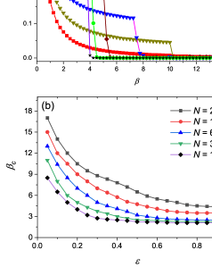
Figure 1: (a) The $\beta$ dependency of large time behavior of final densities $n_{1}$, as the inverse of order parameter in the system, for $\rho_{0}=0.4$. Different energies of $\epsilon$ are shown with different symbols. The system transitions to an ordered state, at some values of $\beta=\beta_{c}$. The system size in all plots is $N=256$. (b) The critical values of $\beta_{c}$ versus $\epsilon$ and for different system sizes $N$. As can be seen, $\beta_{c}$ goes to infinity for large networks or small $\epsilon$.

Figure 2: The time evolution of triad densities, $n_{i}$, with $\epsilon=0.2$ and for initial positive link densities of (a) $\rho_{0}=0.4$ and (b) $\rho_{0}=0.8$. The triad density $n_{1}$ vanishes and thus the system approaches into a stable (weak) balanced state. The dot-dashed lines in both figures indicate the corresponding time evolution of positive link density $\rho$. For all plots, $\beta>\beta_{c}$ (see Fig. 1) and the system size is $N=256$.

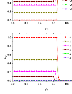
Figure 3: (a) The final positive link density $\rho$ and (b) the final triad density $n_{3}$ versus $\rho_{0}$ for different $\epsilon$. As can be seen, the final fate of the system is a unipolar phase for any arbitrary $\epsilon$ when $\rho_{0}>\rho_{0}^{c}$. For $\rho_{0}\leq\rho_{0}^{c}$, $n$-polar states with $n\geq 2$ emerge. Other parameters are the same as in Fig. 2.

Figure 4: (a) The final positive link density $\rho$ and (b) the final triad density $n_{3}$ versus $\epsilon$ for different $\rho_{0}$. A phase transition from bipolar states into multipolar ones occurs at $\epsilon_{c}\approx 0.67$ when $\rho_{0}\leq\rho_{0}^{c}$. (c) The log-log plot of the mean number of poles versus $\epsilon$ for different values of $\rho_{0}$. For $\rho_{0}\leq\rho_{0}^{c}$, the number of poles decreases as a power law form of $\sim\epsilon^{-0.8}$. Other parameters are the same as in Fig. 2.

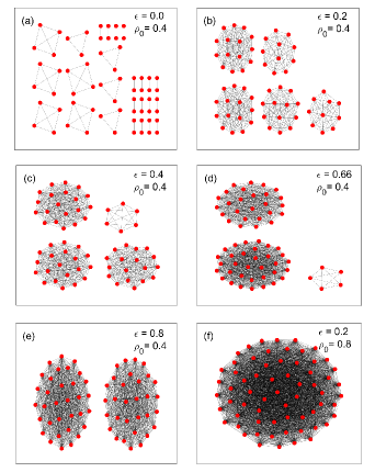
Figure 5: Examples of six final states of the system: (a) to (d) represent multipolarity with different size of the poles. A bipolar and unipolar state are indicated in (e) and (f), respectively. Note that in (a) to (e) $\rho_{0}\leq\rho_{0}^{c}$ and in (f) $\rho_{0}>\rho_{0}^{c}$. The system size is $N=64$ for all graphs. Note that only friendly links are displayed.

III Numerical Results

Initially, we randomly distribute positive and negative links among all nodes so that the initial positive link density $\rho_{0}$ is obtained. Then, we start the dynamics by choosing an arbitrary link, randomly. To check the dependency of the final state of the system on the stochasticity in the individual’s behavior, $\beta$, in Fig. 1(a), we plotted the final values of triads of $n_{1}$ versus different $\beta$ and for different $\epsilon$. By taking into account the density $n_{1}$ as the inverse of order parameter (ordered state = a state without any unfavorable triadic relations, i.e., $n_{1}=0$), we find that for a given $\epsilon$, the system undergoes a phase transition from an unbalanced phase of $n_{1}\neq 0$ into a stable weak balanced state with $n_{1}=0$ as $\beta$ crosses a critical value $\beta_{c}$ from bellow. As can be seen in Fig. 1(b), this critical value $\beta_{c}$ is dependent on the value of the energy $\epsilon$. In fact, as $\epsilon$ decreases, $\beta_{c}$ increases. We note here that the value of $\beta_{c}$ is also dependent on the system size, and diverges for $N\to\infty$. This behavior is consistent with our previous work [23, 26], which can be considered as the special case of $\epsilon=1$ in the present work. This indicates that balanced states (weak or strong) are hardly reached in large systems as well as systems with $\epsilon\to 0$.

To show how the system evolves into a stationary (and stable) state, in Fig. 2, we plot the dynamics of triad densities $n_{0},n_{1},n_{2},n_{3}$ and positive link density $\rho$ for $\epsilon=0.2$ with initial conditions of $\rho_{0}=0.4$ and $0.8$ at $\beta>\beta_{c}$ (here $\beta=1.2\beta_{c}$). The system size here is $N=256$. As can be seen, triads of type $\Delta_{1}$ disappear in all plots, i.e., $n_{1}(\infty)=0$. Thus, the final fate of the system can be three possible states due to the final values of other triad densities: unipolar ($n_{2},n_{3}=0$), bipolar ($n_{2}\neq 0,n_{3}=0$) and mulipolar ($n_{3}\neq 0$). For example, the system approaches into a multipolar state in Fig. 2(a) and a unipolar state emerges in Fig. 2(b). Also, the dot-dashed lines in both plots represent the corresponding final positive link density $\rho$ for both initial densities of $\rho_{0}=0.4$ and $0.8$. To better understand the final states in the system, we present in Fig. 3(a) the final positive link density $\rho_{\infty}$ versus $\rho_{0}$ for different values of $\epsilon$. As can be seen, if $\rho_{0}$ is greater than a critical value of $\rho_{0}^{c}$, the final phase is a unipolar state for all values of $\epsilon$. On the other hand, for $\rho_{0}\leq\rho_{0}^{c}$, multipolar ($n_{3}\neq 0$) and bipolar ($n_{3}=0$) states can emerge for small and large $\epsilon$, respectively as observed in Fig. 3(b) which represents the final densities of $n_{3}$. We note here that this critical value of $\rho_{0}^{c}$ is dependent on $\epsilon$ and we will show later that it is indeed an unstable branch in the phase space of the system.

To better check $\epsilon$ dependency of the final state of the system, we also plot in Fig. 4(a), the final density $\rho_{\infty}$ versus $\epsilon$ for different initial densities $\rho_{0}$. We find again that for $\rho_{0}$ above or bellow the critical value $\rho_{0}^{c}$, the system can reach a unipolar or a multi-bipolar state, respectively. For the case of $\rho_{0}\leq\rho_{0}^{c}$, the fate of the system can be either a bipolar or a multipolar state if the energy $\epsilon$ is larger or smaller than a critical value of $\epsilon^{*}\approx 0.67$, as observed in Fig. 4(b). In fact, for $\epsilon\geq\epsilon^{*}$ the degree of tension associated to triads of type $\Delta_{3}$ is high enough that they cannot survive in the final state of the network. On the other hand, for $\epsilon<\epsilon^{*}$ we find that multipolar states with different sizes emerge. We are also interested in the properties of these emerging multipolar states. For example, Fig. 4(c) demonstrates the mean number of poles $\left\langle N_{pole}\right\rangle$ for different values of initial densities $\rho_{0}$ and energies $\epsilon$, where $\left\langle...\right\rangle$ represents an average over $500$ different realizations of the system. We see that when $\rho_{0}\leq\rho_{0}^{c}$, the mean number of poles decreases as a power law form $\left\langle N_{pole}\right\rangle\sim\epsilon^{-0.8}$ when $\epsilon<\epsilon^{*}$ and remains constant ($\left\langle N_{pole}\right\rangle=2$) if $\epsilon\geq\epsilon^{*}$. Also, for $\rho_{0}>\rho_{0}^{c}$, we have $\left\langle N_{pole}\right\rangle\to 1$ which indicates the unipolarity independent of $\epsilon$. It is noteworthy to mention here that the observed number of poles in real-world systems usually is not large and our results show that this can occur for a reasonable values of energies $\epsilon$ around $0.5$. Finally, in Fig. 5 we present six examples of possible network configurations corresponding to final states of the system for different values of $\epsilon$ and $\rho_{0}$. Indeed, Figs. 5(a) to (d) represent four examples of multipolar states with different pole sizes and Fig. 5(e) indicates a bipolar state. As we mentioned above, a unipolar state emerges for any values of $\epsilon$ when $\rho_{0}>\rho_{0}^{c}$ as indicated in Fig. 5(f). Note that for all Fig. 5(a) to (e), $\rho_{0}\leq\rho_{0}^{c}$ and for Fig. 5(f) $\rho_{0}>\rho_{0}^{c}$.

IV Mean-field approach

Since the system possesses large number of degrees of freedom, its exact time dependent dynamical equations are hard to obtain. In this respect, we search for a mean-field approximation for the rate equations, using the notations used in [15, 23]. As we discussed before, it is appropriate to work with quantity $n_{i}$ which is the density of triads of type $\Delta_{i}$. Another useful quantity is the triad density $n_{i}^{+}$ ($n_{i}^{-}$) of type $\Delta_{i}$ that are connected to a positive (negative) link. $(3-i)N_{i}$ is the total number of positive links connected to triads of type $\Delta_{i}$, and thus the average number of such triads can be obtained as $N_{i}^{+}=(3-i)N_{i}/L_{+}$. Since, each link is connected to $N-2$ triads of any types, thus one can simply find that $n_{i}^{+}=N_{i}^{+}/(N-2)$. Similarly, we can write $n_{i}^{-}=N_{i}^{-}/(N-2)$ for a negative link. Consequently, we have

$$\begin{split}n_{i}^{+}&=(3-i)n_{i}/(3n_{0}+2n_{1}+n_{2})\\ n_{i}^{-}&=in_{i}/(n_{1}+2n_{2}+3n_{3})\end{split}$$ (3)

By considering that $\rho$ is the probability of finding a positive link, the probability of flipping a positive link is $\pi^{+}=p^{+}\rho$, with

$$p^{+}=\frac{1}{1+e^{\beta\Delta U_{+-}}}$$ (4)

and of flipping a negative link is $\pi^{-}=p^{-}(1-\rho)$, with

$$p^{-}=\frac{1}{1+e^{\beta\Delta U_{-+}}}$$ (5)

where $\Delta U_{+-}$ and $\Delta U_{-+}$ are the energy difference due to the flipping a positive and a negative link, respectively. In fact, the transition probabilities $p^{+}$ and $p^{-}$ are the two pivotal parameters that drive the system dynamics.

For an each update at step $j$, we have

$$L_{+}(j+1)-L_{+}(j)=-\pi^{+}+\pi^{-}$$ (6)

Since each time step equals $L$ updates, the rate equation for (average) $\rho$ can be written as

$$\frac{d\rho}{dt}=-\pi^{+}+\pi^{-}$$ (7)

The energy difference due to the flipping of a positive and negative link in each update step equals to $(N_{0}^{+}-N_{1}^{+}+\epsilon N_{2}^{+})/N_{tri}$ and $-(N_{1}^{-}-N_{2}^{-}+\epsilon N_{3}^{-})/N_{tri}$, respectively. Thus we obtain

$$\begin{split}U(j+1)-U(j)=&\pi^{+}(N_{0}^{+}-N_{1}^{+}\\ &+\epsilon N_{2}^{+})/N_{tri}\\ &-\pi^{-}(N_{1}^{-}-N_{2}^{-}\\ &+\epsilon N_{3}^{-})/N_{tri}\end{split}$$ (8)

Therefore, we find the rate equation of the total energy as

$$\frac{dU}{dt}=\pi^{+}\Delta U_{+-}+\pi^{-}\Delta U_{-+}$$ (9)

where

$$\begin{split}\Delta U_{+-}&=+3(n_{0}^{+}-n_{1}^{+}+\epsilon n_{2}^{+})\\ \Delta U_{-+}&=-3(n_{1}^{-}-n_{2}^{-}+\epsilon n_{3}^{-})\end{split}$$ (10)

Also, the rate equations for all triad densities, $n_{i}$, can be obtained in a similar way which are as follows:

$$\begin{split}\frac{dn_{0}}{dt}&=-3\pi^{+}n_{0}^{+}+3\pi^{-}n_{1}^{-}\\ \frac{dn_{1}}{dt}&=-3\pi^{+}n_{1}^{+}-3\pi^{-}n_{1}^{-}+3\pi^{+}n_{0}^{+}+3\pi^{-}n_{2}^{-}\\ \frac{dn_{2}}{dt}&=-3\pi^{+}n_{2}^{+}-3\pi^{-}n_{2}^{-}+3\pi^{+}n_{1}^{+}+3\pi^{-}n_{3}^{-}\\ \frac{dn_{3}}{dt}&=-3\pi^{-}n_{3}^{-}+3\pi^{+}n_{2}^{+}\end{split}$$ (11)

As we mentioned before, the system dynamics are governed by the two transition probabilities of $p^{+}$ and $p^{-}$. In this respect, $p^{+}=p^{-}$ means that the probability of transition of a positive link into a negative one is equal to the transition probability in the reverse direction. For example, if $\beta\to 0$, we have $p^{+}=p^{-}=1/2$, and one can simply find from Eq. 7 that $d\rho/dt=1/2-\rho$ which yields

$$\rho(t)=1/2+(\rho_{0}-1/2)e^{-t}$$ (12)

This demonstrates that for large $t$, $\rho$ tends to $1/2$ as expected in such a fully random situation. However, to find an exact solution for finite $\beta$ is not straightforward, and we will present a qualitative explanation. At first, note that for a finite $\beta$, the relation $\Delta U_{+-}=\Delta U_{-+}$ satisfies the condition $p^{+}=p^{-}$. On the other hand, by assuming that the system remains uncorrelated during its early stages of the evolution, the triad densities become $n_{0}=\rho^{3}$, $n_{1}=3\rho^{2}(1-\rho)$, $n_{2}=3\rho(1-\rho)^{2}$, and $n_{3}=(1-\rho)^{3}$. By substituting these values into Eqs. 3 and 10, we find

$$\Delta U_{+-}=-\Delta U_{-+}=+3\{(3+\epsilon)\rho^{2}-(2+2\epsilon)\rho+\epsilon\}$$ (13)

This relation along with the previous relation of $\Delta U_{+-}=\Delta U_{-+}$, indicates that whenever the positive link density $\rho$ satisfies $\Delta U_{+-}=0$ (or $\Delta U_{-+}=0$), the condition $p^{+}=p^{-}$ is reached. Based on Eq.13, the two solutions of $\Delta U_{+-}=0$ can be obtained as

$$\begin{split}\rho^{\prime}&=((1+\epsilon)-\sqrt{1-\epsilon})/(3+\epsilon)\\ \rho^{\prime\prime}&=((1+\epsilon)+\sqrt{1-\epsilon})/(3+\epsilon)\end{split}$$ (14)

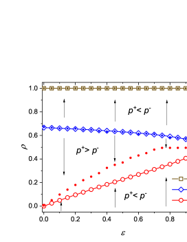
Figure 6: Our analytical solutions obtained by using mean-field approximation. Blue unfilled diamonds, $\rho^{\prime}$, indicates the unstable solution, above and bellow which the system tends to another stable solutions of a unipolar ($\rho^{\prime\prime\prime}$) and a multi-bipolar ($\rho^{\prime\prime}$) state, respectively. The filled symbols represent our simulation results: Diamonds denote the values of phase transition points ($\rho_{0}^{c}$) obtained from Fig. 3(a). Squares and Circles also represent final values of $\rho$ as indicated in Fig. 4(a).

We plotted in Fig. 6, these two solutions for different values of $\epsilon$. Indeed, for $\rho<\rho^{\prime\prime}$, we have $\Delta U_{+-}>0$ (or $\Delta U_{-+}<0$) which means that $p^{+}<p^{-}$. This indicates that negative links will be flipped into positive ones with higher probability, which on average increases $\rho$ until it reaches to $\rho^{\prime\prime}$ where $p^{+}=p^{-}$. By similar mechanism, if $\rho>\rho^{\prime\prime}$ then $p^{+}>p^{-}$, i.e., positive links will change to negative ones with higher probability, and this decreases $\rho$ until it again reaches $\rho^{\prime\prime}$. However, $\rho=\rho^{\prime}$ is an unstable solution, since for $\rho>\rho^{\prime}$, we have $p^{+}<p^{-}$ which increases the number of positive links until $\rho$ reaches its maximum value $\rho=\rho^{\prime\prime\prime}=1$, where $\rho^{\prime\prime\prime}$ is the stable unipolar state. For $\rho<\rho^{\prime}$, we have $p^{+}>p^{-}$ which decreases the number of positive links until $\rho=\rho^{\prime\prime}$. Briefly, our mean-field analysis shows that a bifurcation occurs for $\epsilon<1$, with a stable branch, $\rho^{\prime\prime}$, for $\rho\leq 1/2$ and an unstable branch, $\rho^{\prime}$, for $\rho>1/2$. Filled symbols in Fig. 6 represent our simulation results. In fact, filled diamonds represent values of transition points $\rho_{0}^{c}$ as observed in Fig. 3(a). Filled squares and filled circles also show respectively two final possible states of unipolar and $n$-polar phases with $n\geq 2$ represented in Fig. 3(a) and Fig. 4(a). This demonstrates that our mean-field approximation is mostly in agreement with our numerical simulations, and can well explain the phase space behavior of the system.

V Conclusion

In social balance theory, triads with various interactions are typically grouped into balanced and unbalanced states. Such binary identification may lead to a globally balanced situation which are either uniform or bipolar. On the other hand, many real world situations exhibit multipolarity which have gained much less attention in the literature. In this work, we showed how considering a triad which contains all negative links as less unbalanced than a triad with only one negative link, can lead to an eventual state which contain multipolar communities. Our stochastic dynamics was chosen in accordance with Glauber dynamics in the presence of randomness $\beta$. We described the transition to the multipolar state as a function of $\epsilon$ and $\rho_{0}$ and showed various phase diagrams. The number of final poles crucially depends on the value of $\epsilon$ and can grow very large as $\epsilon$ is reduced considerably. We also provided a mean field calculation which showed how decreasing $\epsilon$ from its standard value leads to a bifurcation with a stable and an unstable branch which was mostly consistent with our numerical simulations. We observed that our model typically leads to multipolar states with roughly homogenous pole size distribution. An interesting question to investigate is the conditions under which a heterogenous size distribution may emerge in a multi-polar society.

References

- Deutsch and Singer [1964] K. W. Deutsch and J. D. Singer, Multipolar power systems and international stability, World Politics 16, 390 (1964).
- Waltz [2010] K. N. Waltz, Theory of international politics (Waveland Press Incorporated, 2010).
- Caves [2004] R. W. Caves, Encyclopedia of the City (Routledge, 2004).
- Schiefer and van der Noll [2016] D. Schiefer and J. van der Noll, The essentials of social cohesion: A literature review, Social Indicators Research 132, 579 (2016).
- Heider [1946] F. Heider, Attitudes and cognitive organization, The Journal of Psychology 21, 107 (1946).
- Cartwright and Harary [1956] D. Cartwright and F. Harary, Structural balance: a generalization of heider’s theory, Psychological Review 63, 277 (1956).
- Harary [1953] F. Harary, On the notion of balance of a signed graph, The Michigan Mathematical Journal 2, 143 (1953).
- Harary [1961] F. Harary, A structural analysis of the situation in the middle east in 1956, Journal of Conflict Resolution 5, 167 (1961).
- Doreian and Mrvar [1996] P. Doreian and A. Mrvar, A partitioning approach to structural balance, Social Networks 18, 149 (1996).
- Szell et al. [2010a] M. Szell, R. Lambiotte, and S. Thurner, Multirelational organization of large-scale social networks in an online world, Proceedings of the National Academy of Sciences 107, 13636 (2010a).
- Szell and Thurner [2010] M. Szell and S. Thurner, Measuring social dynamics in a massive multiplayer online game, Social Networks 32, 313 (2010).
- Facchetti et al. [2011] G. Facchetti, G. Iacono, and C. Altafini, Computing global structural balance in large-scale signed social networks, Proceedings of the National Academy of Sciences 108, 20953 (2011).
- Ilany et al. [2013] A. Ilany, A. Barocas, L. Koren, M. Kam, and E. Geffen, Structural balance in the social networks of a wild mammal, Animal Behaviour 85, 1397 (2013).
- Antal et al. [2006] T. Antal, P. L. Krapivsky, and S. Redner, Social balance on networks: The dynamics of friendship and enmity, Physica D: Nonlinear Phenomena 224, 130 (2006).
- Antal et al. [2005] T. Antal, P. L. Krapivsky, and S. Redner, Dynamics of social balance on networks, Physical Review E 72, 036121 (2005).
- Kułakowski et al. [2005] K. Kułakowski, P. Gawroński, and P. Gronek, The heider balance: A continuous approach, International Journal of Modern Physics C 16, 707 (2005).
- Radicchi et al. [2007] F. Radicchi, D. Vilone, S. Yoon, and H. Meyer-Ortmanns, Social balance as a satisfiability problem of computer science, Physical Review E 75, 026106 (2007).
- Marvel et al. [2011] S. A. Marvel, J. Kleinberg, R. D. Kleinberg, and S. H. Strogatz, Continuous-time model of structural balance, Proceedings of the National Academy of Sciences 108, 1771 (2011).
- Traag et al. [2013] V. A. Traag, P. Van Dooren, and P. De Leenheer, Dynamical models explaining social balance and evolution of cooperation, PloS one 8, e60063 (2013).
- Kulakowski [2007] K. Kulakowski, Some recent attempts to simulate the heider balance problem, Computing in Science and Engineering 9, 80 (2007).
- Hummon and Doreian [2003] N. P. Hummon and P. Doreian, Some dynamics of social balance processes: bringing heider back into balance theory, Social Networks 25, 17 (2003).
- Altafini [2012] C. Altafini, Dynamics of opinion forming in structurally balanced social networks, PloS one 7, e38135 (2012).
- Shojaei et al. [2019] R. Shojaei, P. Manshour, and A. Montakhab, Phase transition in a network model of social balance with glauber dynamics, Physical Review E 100, 022303 (2019).
- Saeedian et al. [2017] M. Saeedian, N. Azimi-Tafreshi, G. R. Jafari, and J. Kertesz, Epidemic spreading on evolving signed networks, Physical Review E 95, 022314 (2017).
- Hassanibesheli et al. [2017] F. Hassanibesheli, L. Hedayatifar, H. Safdari, M. Ausloos, and G. R. Jafari, Glassy states of aging social networks, Entropy 19, 246 (2017).
- Manshour and Montakhab [2021] P. Manshour and A. Montakhab, Reply to “comment on ‘phase transition in a network model of social balance with glauber dynamics’ ”, Physical Review E 103, 066302 (2021).
- Marvel et al. [2009] S. A. Marvel, S. H. Strogatz, and J. M. Kleinberg, Energy landscape of social balance, Physical Review Letters 103, 198701 (2009).
- Facchetti et al. [2012] G. Facchetti, G. Iacono, and C. Altafini, Exploring the low-energy landscape of large-scale signed social networks, Physical Review E 86, 036116 (2012).
- Glauber [1963] R. J. Glauber, Time‐dependent statistics of the ising model, Journal of Mathematical Physics 4, 294 (1963).
- Szell et al. [2010b] M. Szell, R. Lambiotte, and S. Thurner, Multirelational organization of large-scale social networks in an online world, Proceedings of the National Academy of Sciences 107, 13636 (2010b).
- Belaza et al. [2017] A. M. Belaza, K. Hoefman, J. Ryckebusch, A. Bramson, M. van den Heuvel, and K. Schoors, Statistical physics of balance theory, PLoS one 12, e0183696 (2017).
- Davis [1967] J. A. Davis, Clustering and structural balance in graphs, Human Relations 20, 181 (1967).
- Leskovec et al. [2010] J. Leskovec, D. Huttenlocher, and J. Kleinberg, Signed networks in social media, in Proceedings of the SIGCHI conference on human factors in computing systems (2010) pp. 1361–1370.
- Van de Rijt [2011] A. Van de Rijt, The micro-macro link for the theory of structural balance, The Journal of Mathematical Sociology 35, 94 (2011).