scaletikzpicturetowidth[1]

A macroscopic approach for stress driven anisotropic growth in bioengineered soft tissues

^∗ Corresponding author

Abstract. The simulation of growth processes within soft biological tissues is of utmost importance for many applications in the medical sector. Within this contribution we propose a new macroscopic approach fro modelling stress-driven volumetric growth occurring in soft tissues. Instead of using the standard approach of a-priori defining the structure of the growth tensor, we postulate the existance of a general growth potential. Such a potential describes all eligable homeostatic stress states that can ultimately be reached as a result of the growth process. Making use of well established methods from visco-plasticity, the evolution of the growth related right Cauchy-Green tensor is subsequently defined as a time dependent associative evolution law with respect to the introduced potential. This approach naturally leads to a formulation that is able to cover both, isotropic and anisotropic growth related changes in geometry. It furthermore allows the model to flexibly adapt to changing boundary and loading conditions. Besides the theoretical development, we also describe the algorithmic implementation and furthermore compare the newly derived model with a standard formulation of isotropic growth.

Keywords: anisotropic growth, growth potential, engineered tissue, finite strain

Acknowledgements: L. Lamm, J. Jockenvövel and S. Reese gratefully acknowledge the financial support provided by the German Research Foundation (DFG) within the subproject ‘Modelling of the structure and fluid–structure interaction of biohybrid heart valves on tissue maturation’ of the DFG PAK 961 ‘Towards a model based control of biohybrid implant maturation’ (RE 1057/45-1, Project number 403471716). Furthermore, H. Holthusen and S. Reese acknowledge the financial support through the DFG Project ’Experimental and numerical investigation of layered, fiber-reinforced plastics under crash loads’ (RE 1057/46-1, Project number 404502442). L. Lamm, T. Brepols and S. Reese acknowledge the support granted by the AiF through the Project ’Methodology for dimensioning and simulation of adhesive bonds in glass-facade structures’ (IGF 21348 N/3).

1 Introduction

The production and use of artificially grown biological tissue has become an important research topic in the medical context over the last two decades. Great progress has been made in implant research in particular, with the cultivation of biohybrid heart valves being just one example among many (Fioretta et al. [2019]). Designing and constructing highly complex medical implants is a big challenge due to the biomechanical properties of the underlying cultivated tissue. Early works in the field of biomechanics have already pointed out that biological tissues adapt dynamically to the environment they are exposed to (see e.g. Fung [1995] and references therein). The goal of this process is to reach a homeostatic state in which e.g. a certain critical stress state is neither exceeded nor fallen below. During this process, which we will call growth in the following, the progression towards a homeostatic stress state is mainly driven by a change in mass and internal structure of the given biological material. Subsequently, such a growth process leads to a change in the mechanical behaviour, which usually has a large influence on the performance of the given implant. In contrast to native tissue, these adaptive effects are particularly pronounced during the cultivation period of bioengineered tissues and must therefore be taken into account from the beginning of the design process. Within this context, computational modelling contributes to a deeper understanding and prediction of such adaptation processes. An important aspect of modelling the mechanics of growth is the description of geometry changes which are due to contraction and expansion of the material, respectively. Starting from the works of Skalak [1981], Skalak et al. [1982] and Rodriguez et al. [1994], many models have been developed over the last decades in order to describe such finite volumetric growth effects. Although being already successfully applied e.g. in the modelling of finite plasticity (see e.g. Eckart [1948], Kröner [1959], Lee [1969]), it was the contribution of Rodriguez et al. [1994] which first adapted the multiplicative split of the deformation gradient to describe the inelastic nature of finite growth processes. For a detailed overview on the various modelling strategies, the interested reader is referred to the comprehensive overviews given e.g. by Goriely [2017] and Ambrosi et al. [2019]. Most of the approaches based on the conceptually simple and computationally efficient framework by Rodriguez et al. [1994] can be roughly divided into two different groups, isotropic (e.g. Lubarda and Hoger [2002], Himpel et al. [2005]) and anisotropic growth models (e.g. Menzel [2005], Göktepe et al. [2010], Soleimani et al. [2020]). It is important to outline that the distinction between isotropic and anisotropic growth is by no means related to the underlying elastic material behaviour, but rather describes the way a referential volume element changes its shape over time. In case of isotropic growth, the deformation gradient tensor is often assumed to be proportional to the identity tensor (e.g. Lubarda and Hoger [2002]), which yields a uniform expansion of a referential volume element. On the other hand, the term anisotropic growth describes a geometry change of a given volume element that is not uniform in all three spatial dimensions but rather has a distinct growth direction (e.g. Göktepe et al. [2010]). Despite its widespread use, the approach of isotropic growth modelling has strong limitations with regard to describing the mechanical behaviour of complex structures. Recently, Braeu et al. [2017] and Braeu et al. [2019] pointed out that in the context of relevant applications, anisotropic growth behaviour is more the standard case than an isotropic response. Classically, this intrinsically anistropic growth behaviour is modelled using heuristic assumptions on the definition of preferred growth directions. This, unfortunately, yields the need to a-priori prescribe a certain structure of the growth related deformation gradient. Whilst this approach might be feasible for relatively simple problems such as e.g. fibre elongation and contraction, it is not well applicable for more complex applications. It is therefore still an ongoing topic of research to define a more general and flexible formulation that is able to adapt to various boundary value problems, as pointed already out by e.g. Menzel [2005] or Soleimani et al. [2020]. In addition to the phenomenologically motivated models described above, another class of models was established for describing growth processes. Originating from the theory of mixtures, Humphrey and Rajagopal [2002], among others, developed the constrained mixture theory. Instead of assuming that the volume as a whole is deformed during the growth process, this modelling approach describes the change of volume in terms of a continuous deposition and removal of mass increments. Since this approach is computationally very expensive, Cyron et al. [2016] and Cyron and Humphrey [2017] developed a homogenized version of the constrained mixture model. This is achieved by using a temporal homogenization of the mass increments alongside with the same multiplicative split as described by Rodriguez et al. [1994]. Although this approach overcomes the limitations of the classical constrained mixture theory in terms of computational costs, it still suffers from the need to a-priori define the structure of the growth tensor.

As pointed out in the brief literature review above, most existing models in the field of growth simulations require to make assumptions on the structure of the growth tensor. This leads to a situation where growth can always only evolve in a predefined manner. Even if the underlying growth process is the same, this can possibly result in a scenario where the same material subjected to different loading or boundary conditions might need a different constitutive model in order to capture the macroscopical behaviour properly. Consider, e.g., a piece of engineered soft collagenous tissue. It is well known that such a material tends to shrink during its maturation phase, in order to reach homeostasis. The way in which this shrinking process takes place depends very much on the given boundary conditions. While a specimen that is not hindered in its deformation by external boundary conditions clearly exhibits isotropic deformation behaviour, this is no longer the case as soon as, e.g., two sides of the specimen are clamped (see e.g. experiments in Gauvin et al. [2013] and Ghazanfari et al. [2015]). In the authors’ opinion, a constitutive formulation should be developed which is capable of simulating growth processes independently of the given boundary conditions. The present work therefore introduces a novel and flexible framework for the description of stress driven volumetric growth. This framework does not depend on the a-priori definition of the growth tensors structure and is able to cover both, isotropic and anisotropic growth behaviour, naturally. Section 2 covers the theoretical modelling ideas behind the proposed model. The numerical implementation of the derived material model is described in Section 3. Finally, numerical examples are given in Section 4.

2 Continuum mechanical modelling of finite growth

Let us first introduce the well established multiplicative split of the deformation gradient $\mathbf{F}$ into an elastic and a growth related part (see e.g. Rodriguez et al. [1994]), i.e.

$$\mathbf{F}=\mathbf{F}_{e}\mathbf{F}_{g}.$$ (1)

Using this equation, the determinant of $\mathbf{F}$, abbreviated by $J:=\operatorname{det}\mathbf{F}=\operatorname{det}\mathbf{F}_{e}\operatorname{det}\mathbf{F}_{g}$, is also multiplicatively split into two parts. Whilst the change of volume due to elastic deformations is described by $J_{e}=\operatorname{det}\mathbf{F}_{e}$, the growth related volume changes are represented by $J_{g}=\operatorname{det}\mathbf{F}_{g}$. In analogy to the right Cauchy-Green tensor $\mathbf{C}=\mathbf{F}^{T}\mathbf{F}$ as well as the left Cauchy-Green tensor $\mathbf{B}=\mathbf{F}\mathbf{F}^{T}$, the elastic right Cauchy-Green tensor and the growth related right and left Cauchy-Green tensor can be defined as

$$\begin{split}\mathbf{C}_{e}&:=\mathbf{F}_{e}^{T}\mathbf{F}_{e}=\mathbf{F}_{g}^{-T}\mathbf{C}\mathbf{F}_{g}^{-1}\\ \mathbf{C}_{g}&:=\mathbf{F}_{g}^{T}\mathbf{F}_{g}\\ \mathbf{B}_{g}&:=\mathbf{F}_{g}\mathbf{F}_{g}^{T}.\end{split}$$ (2)

Furthermore, the growth related velocity gradient $\mathbf{L}_{g}$ is introduced as

$$\mathbf{L}_{g}=\dot{\mathbf{F}}_{g}\mathbf{F}_{g}^{-1}.$$ (3)

2.1 Balance relations

Growth processes within biological systems in general lead to a change of the systems mass as well as a change of its shape and volume, respectively. Within this contribution, the focus lies on the macroscopic description of changes in shape rather than a change of the systems mass. We therefore neglect the description of the balance of mass in terms of production or flux terms and assume that this balance relation is fulfilled implicitly. It is furthermore well established to assume that growth processes take place on a significantly larger time scale than mechanical deformations do. This standard argument is known as the slow growth assumption and yields for a quasi-static setup of the well known balance of linear momentum

$$\operatorname{Div}\left(\mathbf{F}\mathbf{S}\right)+\mathbf{b}_{0}=\mathbf{0}.$$ (4)

Here $\mathbf{S}$ and $\mathbf{b}_{0}$ denote the second Piola-Kirchhoff stress tensor and the referential body force vector per reference volume, respectively. Following the idea of open system thermodynamics (see e.g. Kuhl and Steinmann [2003] and references therein), we describe the entropy production $\dot{\gamma}$ in terms of the Clausius-Duhem inequality

$$\dot{\gamma}=\mathbf{S}:\frac{1}{2}\dot{\mathbf{C}}-\dot{\psi}+\mathcal{S}_{0}\geq 0,$$ (5)

with the volume specific Helmholtz free energy density $\psi$ defined more precisely in the following section. It is important to notice, that the additional referential entropy sink $\mathcal{S}_{0}$ is introduced to allow for a decrease in entropy due to the growth process itself. Therefore, $\mathcal{S}_{0}$ is never actually computed.

2.2 Helmholtz free energy

We start from the general continuum mechanical framework laid down in Svendsen [2001]. Within this context, the constitutive equations are described with respect to a given but otherwise arbitrary configuration of the material body in question. Similar to the approaches made by Bertram [1999] and Svendsen [2001] in the context of finite plasticity, we choose the elastic part of the Helmholtz free energy to be stated in terms of quantities defined within the so-called grown intermediate configuration.

When modelling finite volumetric growth, it is important to ensure that infinite expansion or shrinkage is avoided. A common approach to tackle this problem is to introduce a set of limiting material parameters, which can be interpreted as the maximum possible growth induced stretches (see e.g. Lubarda and Hoger [2002]). Although such approaches may give computationally reasonable results, this assumption cannot be motivated by underlying physical phenomena. Within the context of growth processes taking place in engineered biological tissues, it is reasonable to assume that a growth related change in volume is always accompanied by a rise in internal pressure. Such pressure accumulations are consequently counteracting the expansion and contraction process, respectively. This growth related internal pressure can be described by including an additional dependency on either $\mathbf{C}_{g}$ or $\mathbf{B}_{g}$. Using the idea of interpreting $\mathbf{F}_{g}$ as a so-called material isomorphism (see e.g. Noll [1958], Svendsen [2001]), it follows that one has to choose $\mathbf{B}_{g}$ in order to ensure that the kinematic quantities are located within the same configuration, i.e.

$$\psi:=\tilde{\psi}\left(\mathbf{C}_{e},\mathbf{B}_{g}\right).$$

Note that this choice is strongly related to the general concept of structural tensors. In the present case, namely by choosing the structural tensor equal to $\mathbf{B}_{g}$, the relation to linear kinematic hardening becomes obvious. This is worked out in the paper of Dettmer and Reese [2004], where linear kinematic hardening is a special case of the so-called Armstrong-Frederick type of kinematic hardening. In the following, we choose an additive format, i.e.

$$\tilde{\psi}:=\psi_{e}(\mathbf{C}_{e})+\psi_{g}(\mathbf{B}_{g}),$$ (6)

for the Helmholtz free energy, where the the both terms are isotropic functions of $\mathbf{C}_{e}$ and $\mathbf{B}_{g}$, respectively. Such an additive split can be motivated easily by the rheological model shown in Figure 1.

Figure 1: Rheological model corresponding to the given volumetric growth model. Growth is denoted by the element including the character $\mathcal{G}$.

This model illustrates nicely that a growth related expansion or contraction directly results in an accumulation of the growth related energy $\psi_{g}$ due to the loading of the associated spring element. Such an increase in growth related energy clearly counteracts the growth deformation and ultimately leads to a decaying growth response. The elastically stored energy $\psi_{e}$ is represented within this rheological model by the second spring element. It is obvious that this particular spring is influenced by both, growth related and purely elastic deformations. Therefore, any deformation associated with the growth element will lead to a change in the elastically stored energy, even under the absence of external loadings.

2.3 Thermodynamic considerations

To derive the constitutive equations representing finite volumetric growth, we next consider the isothermal Clausius-Duhem inequality as given in Equation (5). Inserting the Helmholtz free energy (Equation (6)) and differentiating with respect to time yields

$$\mathbf{S}:\frac{1}{2}\dot{\mathbf{C}}-\left(\frac{\partial\psi_{e}}{\partial\mathbf{C}_{e}}:\dot{\mathbf{C}}_{e}+\frac{\partial\psi_{g}}{\partial\mathbf{B}_{g}}:\dot{\mathbf{B}}_{g}\right)+\mathcal{S}_{0}\geq 0.$$ (7)

By using the product rule as well as utilizing the identities $\dot{\overline{\mathbf{F}_{g}^{-T}}}=-\mathbf{F}_{g}^{-T}\dot{\overline{\mathbf{F}_{g}^{T}}}\mathbf{F}_{g}^{-T}$ and $\dot{\overline{\mathbf{F}_{g}^{-1}}}=-\mathbf{F}_{g}^{-1}\dot{\mathbf{F}}_{g}\mathbf{F}_{g}^{-1}$, the elastic deformation rate can be expressed as

$$\dot{\mathbf{C}}_{e}=\mathbf{F}_{g}^{-T}\dot{\mathbf{C}}\mathbf{F}_{g}^{-1}-\mathbf{L}_{g}^{T}\mathbf{F}_{g}^{-T}\dot{\mathbf{C}}\mathbf{F}_{g}^{-1}-\mathbf{F}_{g}^{-T}\dot{\mathbf{C}}\mathbf{F}_{g}^{-1}\mathbf{L}_{g}.$$ (8)

With the definition of the growth velocity gradient given in Equation (3), the growth related deformation rate can similarly be found as

$$\dot{\mathbf{B}}_{g}=\mathbf{L}_{g}\mathbf{B}_{g}+\mathbf{B}_{g}\mathbf{L}_{g}^{T}.$$ (9)

Combining the equations above and making use of the standard procedure of Coleman and Noll [1963], we can find the thermodynamically consistent definition of the second Piola-Kirchhoff stress tensor as

$$\mathbf{S}=2\mathbf{F}_{g}^{-1}\frac{\partial\psi}{\partial\mathbf{C}_{e}}\mathbf{F}_{g}^{-T}.$$ (10)

Next we introduce the Mandel stress tensor $\mathbf{M}=2\mathbf{C}_{e}\frac{\partial\psi}{\partial\mathbf{C}_{e}}$ and the back-stress tensor $\boldsymbol{\chi}=2\mathbf{B}_{g}\frac{\partial\psi_{2}}{\partial\mathbf{B}_{g}}$. Since the free energy functions $\psi_{e}$ and $\psi_{g}$ are chosen as isotropic function of $\mathbf{C}_{e}$ and $\mathbf{B}_{g}$, respectively, their derivatives $\frac{\partial\psi_{e}}{\partial\mathbf{C}_{e}}$ and $\frac{\partial\psi_{g}}{\partial\mathbf{B}_{g}}$ are symmetric and commute with either $\mathbf{C}_{e}$ or $\mathbf{B}_{g}$. Combining this with the properties of the double contracting product, the reduced Clausius-Duhem inequality can be written only in terms of the symmetric part $\mathbf{D}_{g}=\operatorname{sym}\mathbf{L}_{g}$ of the growth velocity gradient, i.e.

$$\dot{\gamma}_{red}=\left[\mathbf{M}-\boldsymbol{\chi}\right]:\mathbf{D}_{g}+\mathcal{S}_{0}\geq 0.$$ (11)

Similar to classical plasticity theory, see e.g. Vladimirov et al. [2008], one can identify the Mandel stress tensor $\mathbf{M}$ and the back-stress tensor $\boldsymbol{\chi}$ as the conjugated driving forces for the evolution of growth. It is therefore natural to describe the evolution equation for $\mathbf{D}_{g}$ in terms of these quantities. Notice that $\mathbf{M}$ and $\boldsymbol{\chi}$ are located within a grown intermediate configuration, where they can be clearly identified as stress like quantities. This becomes clear by the fact that $\mathbf{M}$ has the same invariants as the Kirchhoff stress tensor $\boldsymbol{\tau}$ and, thus, has a clear physical meaning (see Appendix A.1). Pulling $\mathbf{M}$ and $\boldsymbol{\chi}$ back to the reference configuration will yield a loss of such clear physical interpretation. Nevertheless, from a conceptual and computational point of view, a pull back of of these quantities to the reference configuration is desirable (for details see e.g. Dettmer and Reese [2004] and Vladimirov et al. [2008]). Taking into account the relation $\mathbf{D}_{g}=\frac{1}{2}\mathbf{F}_{g}^{-T}\dot{\mathbf{C}}_{g}\mathbf{F}_{g}^{-1}$ one can rewrite the Clausius Duhem inequality purely in terms of quantities located within the reference configuration, i.e.

$$\begin{split}\dot{\gamma}_{red}&=\left(\mathbf{F}_{g}^{-1}\mathbf{M}\mathbf{F}_{g}^{-T}-\mathbf{F}_{g}^{-1}\boldsymbol{\chi}\mathbf{F}_{g}^{-T}\right):\frac{1}{2}\dot{\mathbf{C}}_{g}+\mathcal{S}_{0}\\ &=\left(\mathbf{\Gamma}-\mathbf{X}\right):\frac{1}{2}\dot{\mathbf{C}}_{g}+\mathcal{S}_{0}\\ &=\mathbf{\Sigma}:\frac{1}{2}\dot{\mathbf{C}}_{g}+\mathcal{S}_{0}\geq 0.\end{split}$$ (12)

Similar to the formulation given with respect to the grown intermediate configuration, it is reasonable to define the evolution of the growth related right Cauchy-Green tensor $\mathbf{C}_{g}$ in terms of the thermodynamically conjugated driving forces $\mathbf{\Gamma}=\mathbf{C}_{g}^{-1}\mathbf{C}\mathbf{S}$ and $\mathbf{X}=2\frac{\partial\psi_{g}}{\partial\mathbf{C}_{g}}$. It is important to mention that using $\mathbf{C}_{g}$ as the internal variable yields the fact that $\mathbf{F}_{g}$ must never be computed in the first place. Such an approach is in clear contrast to the standard formulations in volumetric growth modelling, where the the growth tensor itself is usually explicitly prescribed.

2.4 Evolution of growth

Up to this point, the framework presented is very general and could be used to describe a wide variety of inelastic phenomena in finite deformations. It is therefore the choice of evolution equations for $\mathbf{C}_{g}$ that explicitly defines a particular kind of inelastic material model. For the most simple modelling assumption of a purely isotropic growth response, the inelastic part of the deformation gradient is usually defined as $\mathbf{F}_{g}=\vartheta\mathbf{I}$, where $\vartheta$ describes the growth induced stretch (see e.g. Lubarda and Hoger [2002], Himpel et al. [2005], Göktepe et al. [2010]). Using the thermodynamic framework described above, this assumption naturally leads to an evolution equation of $\mathbf{C}_{g}$, which can be written as

$$\dot{\mathbf{C}}_{g}:=2\frac{\dot{\vartheta}}{\vartheta}\mathbf{C}_{g}.$$ (13)

Within this context, a scalar valued evolution equation $\dot{\vartheta}=f(\vartheta,\mathbf{\Sigma},...)$ is used to determine the overall growth response (see Appendix A.2 for a more detailed example). Although the a priori assumption of $\mathbf{F}_{g}$ being a diagonal tensor is tempting due to its computational simplicity, it was already pointed out in various publications that such an assumption is not reasonable for many applications (see e.g. Soleimani et al. [2020], Braeu et al. [2019], Braeu et al. [2017]). This is especially the case for scenarios in which the body cannot grow freely but is restricted by complex boundary conditions. To overcome this issue, a new volumetric growth model is proposed in the following.

2.4.1 Finite growth using a growth potential

As described in the introduction, cell mediated expansion or compaction of engineered tissues takes place in such a way that a preferred homeostatic stress state is reached within the material. In the present work, it is assumed that this homeostatic state can be described in terms of a scalar equivalent stress. Thus, growth always takes place, if this equivalent stress is not equal to the preferred stress state of the biological material. These considerations lead us to the introduction of a general growth potential

$$\Phi:=\tilde{\Phi}\left(\mathbf{M},\boldsymbol{\chi},\alpha_{1},...,\alpha_{n}\right),$$ (14)

which is a function of the conjugated driving forces as well as a set of material parameters $\alpha_{i}$. Similar to the representation used in classical plasticity theory, this potential can be represented as a surface, located within the principal stress space, which contains all eligible homeostatic stress states. It will therefore be named homeostatic surface in the following. An example for such a homeostatic surface can be found in Figure 2. The overall goal of this process is to approach $\Phi=0$ over time and therefore reach a stress state that lies on the homeostatic surface. Furthermore, it seems natural that such growth processes always try to minimize the amount of energy needed to reach the homeostatic state. Hence, the direction of growth response will be described by as the derivative of the growth potential, i.e. $\mathbf{N}=\frac{\partial\Phi}{\partial\mathbf{M}}$. It is furthermore obvious that homeostasis is never reached instantaneously but rather approached over a certain period of time. To account for this temporal effect, we introduce the growth multiplier $\dot{\lambda}_{g}:=\dot{\lambda}_{g}\left(\Phi,\eta,\beta_{1},...,\beta_{n}\right)$ defined as an explicit function of the growth potential, the growth velocity $\eta$ and a set of material parameters $\beta_{i}$. Subsequently, the considerations above lead us to an associative growth evolution law that is postulated as

$$\mathbf{D}_{g}:=\dot{\lambda}_{g}\frac{\mathbf{N}}{||\mathbf{N}||}.$$ (15)

In general, we do not want to restrict the choice of $\Phi$ to only positive homogeneous potentials of degree one. This has the side effect that $||\mathbf{N}||=1$ can not be guaranteed, which yields the need to normalize the growth direction tensor to assure that only $\dot{\lambda}_{g}$ has an influence on the amount of accumulated growth deformations. As before, we furthermore can define the given evolution equation in terms of quantities located purely within the reference configuration. To achieve this, a pull back operation is performed that yields

$$\dot{\mathbf{C}}_{g}=\frac{2\dot{\lambda}_{g}}{||\mathbf{N}||}\mathbf{F}_{g}^{T}\mathbf{N}\mathbf{F}_{g}=\dot{\lambda}_{g}\mathbf{f}=\dot{\lambda}_{g}\mathbf{g}\mathbf{C}_{g},$$ (16)

including the general second order tensors $\mathbf{f}=\frac{2}{||\mathbf{N}||}\mathbf{F}_{g}^{T}\mathbf{N}\mathbf{F}_{g}$ as well as $\mathbf{g}=\mathbf{f}\mathbf{C}_{g}^{-1}$.

Remark.

The same result for Equation (16) could also be obtained following Reese et al. [2021] and the procedures proposed therein. Therefore, this evolution law could be interpreted in the broader context of a theory describing the evolution of general structural tensors.

Since this approach is very similar to the classical models of visco-plasticity, the attentive reader may ask how far these approaches differ. In the case of plasticity, the yield criterion is used to clearly distinguishe between the purely elastic and elasto-plastic state, i.e. the yield criterion must always be less than or equal to zero. In contrast, the growth potential $\Phi$ does not serve to distinguish between an elastic and inelastic region, since an ’elasto-growth’ state is present for both $\Phi<0$ and $\Phi>0$. Only in case of $\Phi=0$ no further growth has to take place, since homeostasis has already been reached. This behaviour is also reflected by the growth multiplier, which in contrast to plasticity can also have negative values. In the authors opinion this modelling approach has several advantages: (i) As stated earlier, the direction of growth does not have to be a priori prescribed, (ii) the complexity of the material model is reduced and (iii) due to the strong similarities to plasticity, one can rely on a large repertoire of knowledge from this field, both from a modeling and numerical point of view. For instance, one could argue that the preferred stress can not only be described by only one smooth growth potential. Having e.g. the concept of multisurface plasticity in mind, it would be easy to adopt the growth potential by a more sophisticated approach. In addition, it is also possible, for instance, to take into account a changing preferred stress using an approach similar to the concept of isotropic hardening.

Before defining a specific form of the growth potential, we first take a closer look at the structure of such a potential. It has already been pointed out above that it is reasonable to assume that growth in biological tissues tends to be of isotropic nature only in the absence of restricting boundary conditions. This idea leads us to the definition of the growth potential as a function of the volumetric invariant $I_{1}:=\operatorname{tr}\left(\mathbf{M}-\boldsymbol{\chi}\right)=\operatorname{tr}\left(\mathbf{\Sigma}\mathbf{C}_{g}\right)$. To allow also for an anisotropic growth response, we furthermore include the deviatoric invariant $J_{2}:=\frac{1}{2}\operatorname{tr}\left(\operatorname{dev}\left(\mathbf{M}-\boldsymbol{\chi}\right)^{2}\right)=\frac{1}{2}\operatorname{tr}\left(\operatorname{dev}\left(\mathbf{\Sigma}\mathbf{C}_{g}\right)^{2}\right)$ (see Appendix A.3). With theses considerations at hand, we propose a general form for the growth potential as

$$\Phi:=\Phi\left(I_{1},J_{2},\omega_{hom}\right)=\phi_{1}\left(I_{1}\right)+\phi_{2}\left(J_{2}\right)-\omega_{hom}.$$ (17)

Here, the material parameter $\omega_{hom}$ describes a stress like quantity defining the state of homeostasis. It is important to emphasize that the combination of $I_{1}$ and $J_{2}$ is crucial for the proposed material model. If the potential was merely defined in terms of the volumetric invariant $I_{1}$, the growth direction tensor would become proportional to the identity tensor which consequently yields an evolution equation that is similar to the isotropic evolution law given in Equation (13). It is the dependency on $J_{2}$ that introduces an anisotropic growth behaviour, since the growth direction tensor no longer necessarily has to correspond to the identity. Nevertheless, in case of purely volumetric stress states, the dependency on $I_{1}$ ensures the desired isotropic growth response. This consideration yields an exclusion of any purely deviatoric potential, e.g. of von Mises type potentials. Furthermore, any suitable potential must fulfill $\frac{\partial\Phi}{\partial\mathbf{M}}\neq\mathbf{0}$ for all $\left(\mathbf{M}-\boldsymbol{\chi}\right)\in\left(\mathbb{R}^{3}\times\mathbb{R}^{3}\right)$ in order to guarantee a well-defined growth direction for any arbitrary loading condition.

2.4.2 Choice of the growth potential and growth multiplier evolution

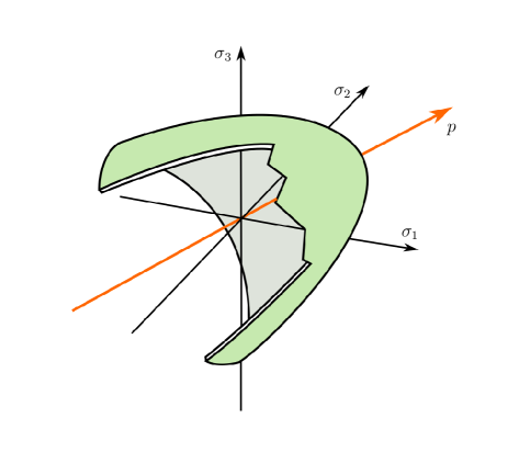
(a) Homeostatic surface located in principal stress space.

(b) Intersection of homeostatic surface with $\sigma_{1}=\sigma_{2}$, showing the influence of the material parameter $m$ for $m_{i}<1$ with $m_{1}<m_{2}<m_{3}$.

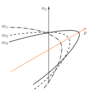
(c) Intersection of homeostatic surface with $\sigma_{1}=\sigma_{2}$, showing the influence of the material parameter $m$ for $m_{i}>1$ with $m_{1}<m_{2}<m_{3}$.

Figure 2: Schematic representation of the homeostatic surface defined by the growth potential from Equation (18) displayed in principal stress space. The hydrostatic axis $p=\operatorname{tr}\left(\mathbf{M}-\boldsymbol{\chi}\right)$ is shown in orange. The eigenvaules of $\mathbf{M}-\boldsymbol{\chi}$ are denoted by $\sigma_{i}$.

The form of a specific potential depends strongly upon the needs of the given application. Unfortunately, there is currently a lack of meaningful experimental data regarding the mechanics of volumetric growth. We therefore choose a potential that proofed to be able to predict our macroscopical observations and further satisfies the general requirements stated above. For this purpose, the quadratic potential as described e.g. by Stassi-D’Alia [1967] and Tschoegl [1971] is used in the following. This potential can be expressed in terms of $\omega_{hom}=m\sigma_{g}^{2}$ including the material parameters $m$ and $\sigma_{g}$, i.e.

$$\Phi=3J_{2}-(1-m)\sigma_{g}I_{1}-m\sigma_{g}^{2}.$$ (18)

As shown in Figure 2(a), the homeostatic state defined by this particular growth potential forms a hyperbolic surface within the principal stress space. The tipping point of this parabola is located on the hydrostatic axis, where its precise location is determined by the parameter $m$ (see Figures 2(b) and 2(c)). From Equation (18) it is obvious that both parameters must always be greater than zero. It is furthermore important to notice that the opening side of the parabolic potential lies within the compressive regime for $m<1$ and in the tensional regime for $m>1$, respectively. Since a choice of $m=1$ describes a von-Mises type model such a choice of this parameters must be avoided. Using this specific form of the growth potential yields the growth direction tensor as

$$\mathbf{N}=\mathbf{F}_{g}\left(3\operatorname{dev}\left(\mathbf{\Sigma}\mathbf{C}_{g}\right)-\left(1-m\right)\sigma_{g}\mathbf{I}\right)\mathbf{F}_{g}^{-1}.$$ (19)

To complete the set of equations needed to describe the evolution of the growth related right Cauchy-Green tensor, we furthermore define a particular form for the evolution of the growth multiplier $\dot{\lambda}_{g}$. From a physically motived point of view, it seems natural that the growth response increases with the deviation of the current stress state from homeostasis. We therefore assume the change in accumulated growth stretch is proportional to the current value of the growth potential. This furthermore ensures that the growth process stops as soon as homeostasis is reached. With these assumptions in mind, we choose the well established approach proposed in Perzyna [1966] and Perzyna [1971], i.e.

$$\dot{\lambda}_{g}:=\frac{1}{\eta}\left(\frac{\Phi}{m\sigma_{g}^{2}}\right)^{\frac{1}{\nu}}.$$ (20)

Herein the growth multiplier is defined in terms of the growth relaxation time $\eta$ as well as a non-linearity parameter $\nu$.

2.4.3 Choice of Helmholtz free energy

Until this point, the constitutive framework presented herein has been described without defining a particular form of the Helmholtz free energy. In general, the choice of the energy potential depends upon the specific type of material one would want to model. For the time being, we choose a compressible Neo-Hookean type model to describe the elastic response of the material. Therefore, the elastic energy $\psi_{e}$ is written in terms of the Lamé constants $\mu$ and $\Lambda$ as

$$\psi_{e}=\frac{\mu}{2}\left(\operatorname{tr}\mathbf{C}_{e}-3\right)-\mu\operatorname{ln}J_{e}+\frac{\Lambda}{4}\left(J_{e}^{2}-1-2\operatorname{ln}J_{e}\right).$$ (21)

Following the argumentation in Section 2.2, we furthermore define the growth related Helmholtz free energy $\psi_{g}$ in terms of a stiffness like material parameter $\kappa_{g}$ such that

$$\psi_{g}=\frac{\kappa_{g}}{2}\left(J_{g}^{2}-1-2\operatorname{ln}J_{g}\right).$$ (22)

This particular choice of the growth related energy obviously fulfills the general requirements for the definition of a strain energy density, i.e. $\psi_{g}(J_{g}\rightarrow 0)\rightarrow\infty$ as well as $\psi_{g}(J_{g}=1)=0$ and $\psi_{g}(J_{g}\rightarrow\infty)\rightarrow\infty$. With these definitions at hand the second Piola-Kirchhoff stress tensor and the back-stress tensor can be derived as

$$\begin{split}\mathbf{S}&=\mu\left(\mathbf{C}_{g}^{-1}-\mathbf{C}^{-1}\right)+\frac{\Lambda}{2}\left(\left(\frac{J}{J_{g}}\right)^{2}-1\right)\mathbf{C}^{-1}\\ \mathbf{X}&=\kappa_{g}\left(J_{g}^{2}-1\right)\mathbf{C}_{g}^{-1}\end{split}$$ (23)

Notice that the conjugated driving force $\mathbf{\Gamma}$ can be easily computed, if $\mathbf{C}_{g}$ and $\mathbf{S}$ are known (see Section 2.3).

3 Numerical implementation

To incorporate the volumetric growth model at hand into a finite element simulation framework, a suitable time integration technique has to be used for evolution equation (16). As shown for example by Weber and Anand [1990], Simo [1992], Reese and Govindjee [1998], Vladimirov et al. [2008] and discussed in further detail by Korelc and Stupkiewicz [2014], the exponential mapping algorithm is a very suitable choice for the treatment of the given evolution equation. We will therefore briefly describe this approach in the following.

Starting with the introduction of discrete time increments $\Delta t=t_{n+1}-t_{n}$ together with the growth increments $\Delta\lambda_{g}=\Delta t\dot{\lambda}_{g}$, the exponential integration scheme for the evolution Equation (16) can be written as

$$\mathbf{C}_{g_{n+1}}=\operatorname{exp}\left(\Delta\lambda_{g}\mathbf{g}\right)\mathbf{C}_{g_{n}}.$$ (24)

Notice, that subscript $n+1$ will be dropped in the following for notational simplicity, which means that any discrete quantity without subscript will be associated with the current time step. Following the argumentation within Vladimirov et al. [2008] and Dettmer and Reese [2004] Equation (24) can be reformulated to ensure the symmetry of $\mathbf{C}_{g}$. Furthermore, the authors mentioned above show that the exponential function within this equation can be expressed in terms of the growth related right stretch tensor $\mathbf{U}_{g}=\sqrt{\mathbf{C}_{g}}$. Consequently, this leads to the discretized evolution equation given as

$$\mathbf{C}_{g_{n}}^{-1}=\mathbf{U}_{g}^{-1}\operatorname{exp}\left(\Delta\lambda\mathbf{U}_{g}^{-1}\mathbf{f}\mathbf{U}_{g}^{-1}\right)\mathbf{U}_{g}^{-1}.$$ (25)

In order to complete the set of discrete constitutive equations, the discrete growth multiplier $\Delta\lambda_{g}$ must determined. This can be achieved by reformulating Equation (20) (see e.g. Simo and Hughes [1998] and de Souza Neto et al. [2008]), i.e.

$$\Phi=m\sigma_{g}^{2}\left(\Delta\lambda_{g}\eta\right)^{\nu}.$$ (26)

Since both of the discrete constitutive equations are non-linear in their arguments, a local iterative solution algorithm must be applied at integration point level to solve for both, the internal variable $\mathbf{U}_{g}^{-1}$ as well as the growth increment $\Delta\lambda_{g}$. It is convenient for such algorithms to write the evolution equations in terms of a set of coupled residual functions, which read in the case of this material model

$$\begin{split}\mathbf{r}_{g}&=-\mathbf{C}_{g_{n}}^{-1}+\mathbf{U}_{g}^{-1}\operatorname{exp}\left(\Delta\lambda\mathbf{U}_{g}^{-1}\mathbf{f}\mathbf{U}_{g}^{-1}\right)\mathbf{U}_{g}^{-1}=\mathbf{0}\\ r_{\Phi}&=\Phi-m\sigma_{g}^{2}\left(\Delta\lambda_{g}\eta\right)^{\nu}=0.\end{split}$$ (27)

Due to the symmetry of $\mathbf{U}_{g}$, the tensor valued residual function $\mathbf{r}_{g}$ can be transformed into Voigt notation, which is computationally more efficient than solving the full tensorial equation. When applying a Newton-Raphson procedure to solve Equations (27), the increments of the equations arguments can be found by solving a linearized system of equations, i.e.

$$\begin{pmatrix}\frac{\partial\hat{\mathbf{r}}_{g}}{\partial\hat{\mathbf{U}}_{g}}&\frac{\partial\hat{\mathbf{r}}_{g}}{\partial\Delta\lambda_{g}}\\ \frac{\partial r_{\Phi}}{\partial\hat{\mathbf{U}}_{g}}&\frac{\partial r_{\Phi}}{\partial\Delta\lambda_{g}}\\ \end{pmatrix}\Delta\begin{pmatrix}\hat{\mathbf{U}}_{g}\\ \Delta\lambda_{g}\end{pmatrix}=-\begin{pmatrix}\hat{\mathbf{r}}_{g_{n}}\\ r_{\Phi_{n}}\end{pmatrix}.$$ (28)

During the solution process, these increments are recomputed for every iteration step in which they are used to update the local iteration procedure. The partial derivatives used herein are not computed analytically but rather calculated by means of an algorithmic differentiation approach. For this, the software package AceGen, as described e.g. in Korelc [2002] and Korelc [2009], is being used to automatically generate source code for the computation of the tangent operators.

Since the local material response is implicitly included within the global material tangent operator of a finite element simulation, we furthermore need to derive this tangent in a consistent manner. Otherwise, quadratic convergence of the global iteration scheme would not be reached. For this, one should bear in mind that the second Piola-Kirchhoff stress is a function of the right Cauchy-Green tensor as well as the internal variables. Within the given framework, the material tangent operator can be expressed as

$$\mathbb{C}=2\left(\left.\frac{\partial\mathbf{S}}{\partial\mathbf{C}}\right|_{\mathbf{U}_{g}}+\left.\frac{\partial\mathbf{S}}{\partial\mathbf{U}_{g}}\right|_{\mathbf{C}}:\frac{\partial\mathbf{U}_{g}}{\partial\mathbf{C}}\right).$$ (29)

Similar to the local tangent operator, these partial derivatives are computed using the software package AceGen. For this, the partial derivative of the growth related stretch tensor $\mathbf{U}_{g}$ with respect to the right Cauchy Green tensor can be determined from the following relation

$$\Delta\begin{pmatrix}\hat{\mathbf{U}}_{g}\\ \Delta\lambda_{g}\end{pmatrix}=-\begin{pmatrix}\frac{\partial\hat{\mathbf{r}}_{g}}{\partial\hat{\mathbf{U}}_{g}}&\frac{\partial\hat{\mathbf{r}}_{g}}{\partial\Delta\lambda_{g}}\\ \frac{\partial r_{\Phi}}{\partial\hat{\mathbf{U}}_{g}}&\frac{\partial r_{\Phi}}{\partial\Delta\lambda_{g}}\\ \end{pmatrix}^{-1}\begin{pmatrix}\frac{\partial\hat{\mathbf{r}}_{g}}{\partial\hat{\mathbf{C}}}\\ \frac{\partial r_{\Phi}}{\partial\hat{\mathbf{C}}}\end{pmatrix}\Delta\hat{\mathbf{C}}.$$ (30)

Here, we reuse the fully converged residual and jacobian from the local solution process. Then, the desired partial derivative is given as the corresponding $6\times 6$ submatrix located in the upper left corner of the right-hand side matrix product.

4 Numerical examples

In the following section, numerical examples are presented to examine and discuss various aspects of the material model introduced above. Since there is a lack of meaningful experimental data describing the volumetric growth in bioengineered tissues, the material parameters used for the presented studies are chosen by means of an educated guess. First, we show the influence of boundary conditions on the development of the volumetric growth process using a simple block model. For this purpose, volumetric growth in the absence of geometrically constraining boundary conditions is evaluated as well as the impact of both, temporal constant and time dependent constraining boundary conditions. Next, we investigate the influence of the introduced set of material parameters, before showing structural examples of a shrinking tissue stripe and comparing its growth related response to an isotropic growth formulation. For the finite element simulations, we implemented the presented material model as well as the element formulation itself into the FEAP software package (Taylor and Govindjee [2020]) in terms of a user-element routine. For meshing and visualization of the structural examples we have used the open source software tools GMSH (Geuzaine and Remacle [2009]) and Paraview (Ahrens et al. [2005]). Furthermore, the open source parallelisation tool GNU Parallel (Tange [2011]) was used during evaluations of the examples shown below.

Figure 3: Geometrical block model with uniform side length of $1~{}\text{mm}$. Uniaxial boundary conditions are given in gray and time dependent displacement $u_{z}(t)$ is denoted in red. Evaluation points $P_{1}=(1,1,1)$ and $P_{2}=(1,1,0.5)$ are given in blue.

	$\mu$	$\Lambda$	$\kappa_{g}$	$m$	$\sigma_{g}$	$\eta$	$\nu$
	$\left[\frac{\text{N}}{\text{mm}^{2}}\right]$	$\left[\frac{\text{N}}{\text{mm}^{2}}\right]$	$\left[\frac{\text{N}}{\text{mm}^{2}}\right]$	$\left[-\right]$	$\left[\frac{\text{N}}{\text{mm}^{2}}\right]$	$\left[\text{s}\right]$	$\left[-\right]$
Geom. unconstrained growth	40	400	150	1.2	70	20	1.0
Geom. constrained growth	40	400	250	1.2	200	100	1.0
Clamped tissue stripe	100	800	150	2.0	250	100	1.0

Table 1: Material parameters for numerical examples

4.1 Geometrically unconstrained growth

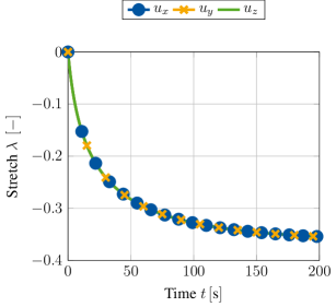
Figure 4: Isotropic growth behaviour resulting in a uniform contraction in all three spatial dimensions. No constraining boundary conditions are applied (i.e. no $u_{z}(t)$). Stretches are evaluated at point $\text{P}_{1}$ (see Figure 3).

As a first example, we use the geometrical model shown in figure 3 without applying any time dependent displacement boundary condition $u_{z}(t)$. Therefore, the specimen is able to expand or contract freely throughout the whole simulation, which should result in an isotropic growth response. We furthermore use the set of material parameters given in Table 1. The growth response for a choice of $m=1.2$ is visualized in Figure 4. Shown by the stretches of point $\text{P}_{1}$ located in the upper corner of the given block geometry, it is obvious that the specimen contracts as expected. Since no constraining boundary conditions are applied, the overall stress within this system should always be equal to zero and therefore could never reach a state of tensional homeostasis. It is the additional growth related free energy, which leads to the limitation of the otherwise infinite shrinking process. One can observe this influence really well in Figure 5(a), where lower values of $\kappa_{g}$ lead to a more pronounced shrinking of the specimen. It is worth noticing that $\kappa_{g}>0$ must hold for any simulation, since neglecting the contribution of internal pressures would lead to non physical behaviour and consequently to an unstable simulation.

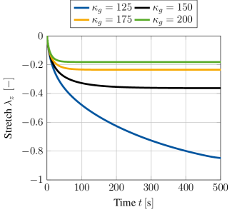
(a) Various choices of the material parameter $\kappa_{g}$.

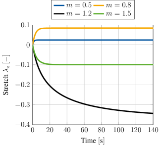
(b) Various choices of the material parameter $m$.

(c) Various choices of the material parameter $\sigma_{g}$.

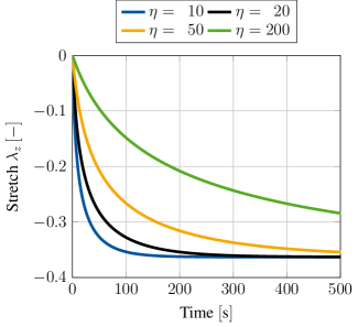
(d) Various choices of the material parameter $\eta$.

Figure 5: Growth induced stretch due to contraction of a block specimen for various sets of material parameters. No constraining boundary conditions are applied (i.e. no $u_{z}(t)$). Stretches are evaluated at point $\text{P}_{1}$ (see Figure 3).

It is furthermore shown in Figure 5(d) that the growth rate parameter $\eta$ has only an impact on the speed at which the volumetric growth process approaches the desired homeostatic state but not on its magnitude. However, as shown in Figures 5(b) and 5(c) a change in magnitude of the homeostatic state can be achieved by variation of $m$ and $\sigma_{g}$. As already described in Section 2.4.2, the material parameter $m$ defines the location of the growth potential’s tipping point on the hydrostatic axis. For values of $m<1$ this point lies in the compressive regime, whilst a choice of $m>1$ pushes this point into the tension regime. As a result, the specimen approaches homeostasis either by expansion or by shrinkage. This behaviour is really well reflected within Figure 5(b). It is furthermore important to point out that for a choice of $m=1$ the homeostatic potential introduced in Equation (18) becomes a von Mises type criterion, which must not be applied due to its purely deviatoric nature. Therefore, this particular choice of $m$ should be avoided when using the potential introduced above.

4.2 Geometrically constrained growth

(a)

(b)

Figure 6: Evolution of Cauchy stress $\sigma_{zz}$ and growth multiplier $\Delta\lambda_{g}$ during stepwise loading of block specimen with $u_{z}(t)$. Both quantities are evaluated at point $\text{P}_{1}$(Figure 3). Right: The stress response is always converging towards a homeostatic state. This state is slightly different, after coming out of the compressive regime. This can be explained by the accumulted internal pressures described by the energy $\psi_{g}$. Left: Growth multiplier indicating, that the specimen is either expanding or shrinking to reach homeostasis.

For the next example, we choose a stepwise time dependent displacement $u_{z}(t)$ to which the block given in Figure 3 is subjected. For the first $250$ time steps, the displacement is held constant at $u_{z}(t)=0~{}\text{mm}$ before being raised to $u_{z}(t)=0.3~{}\text{mm}$ and held constant for another $200$ time steps. Next, we apply compression by setting $u_{z}(t)=-0.1~{}\text{mm}$ and holding it constant for another $250$ time steps. At last, $u_{z}(t)$ is reset to zero again. The material parameters for this example are given in Table 1.

When applying this stepwise alternating stretch to the given block specimen, it can be seen in Figure 6 that the material shrinks and expands depending on the current loading state, respectively. During the first loading period, the accumulated Cauchy stress $\sigma_{zz}$ rises to a value of approximately $300~{}\text{MPa}$, which is due to a contraction induced by the volumetric growth process. This effect is represented by the evolution of the growth multiplier as shown in Figure 6(a). Since the multiplier is negative, the specimen approaches homeostasis by shrinking. Once the displacement is raised to $u_{z}(t)=0.3~{}\text{mm}$, the Cauchy stress $\sigma_{zz}$ also rises abruptly before decaying and approaching the same homeostatic stress state as before. This kind of stress reduction is achieved by an expansion of the specimen, which is represented by a positive value of the growth multiplier. The following compression of the specimen causes a negative jump in the overall stress response. This again induces shrinkage of the specimen in order to regain the homeostatic state of approximately $300~{}\text{MPa}$. It is important to notice that this homeostatic state is slightly higher than the state reached in the loading cycles before. This change is due to the accumulated internal pressures described by the growth related energy $\psi_{g}$. Consequently, this results in a shift of the homeostatic surface similar to kinematic hardening in plasticity. To what extent this effect corresponds to experimental studies is still unclear due to the lack of available data. However, there is no question that this effect can be adapted to any experimental data without further problems by extending the model, e.g. by a non-linear formulation. When setting $u_{z}(t)=0~{}\text{mm}$ in the last loading cycle, the Cauchy stresses overshoot this new homeostatic state slightly. This again results in an expansion of the specimen in order to release the excessive stresses.

4.3 Growth of a clamped tissue stripe

(a) Full structure

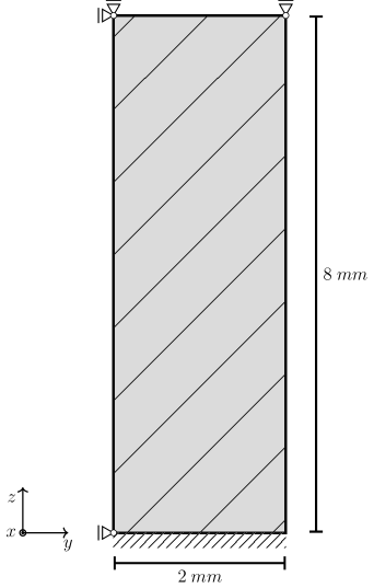
(b) Symmetric part

Figure 7: Geometric model of clamped tissue stripe with thickness of $t=2~{}\text{mm}$. The overall structure is also supported in the $x$ direction.

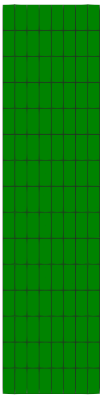
(a) 360 el.

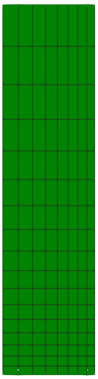
(b) 408 el.

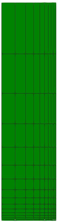
(c) 450 el.

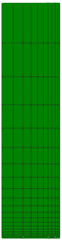
(d) 1000 el.

(e) 3000 el.

(f) Close up of right corner for 450 el.

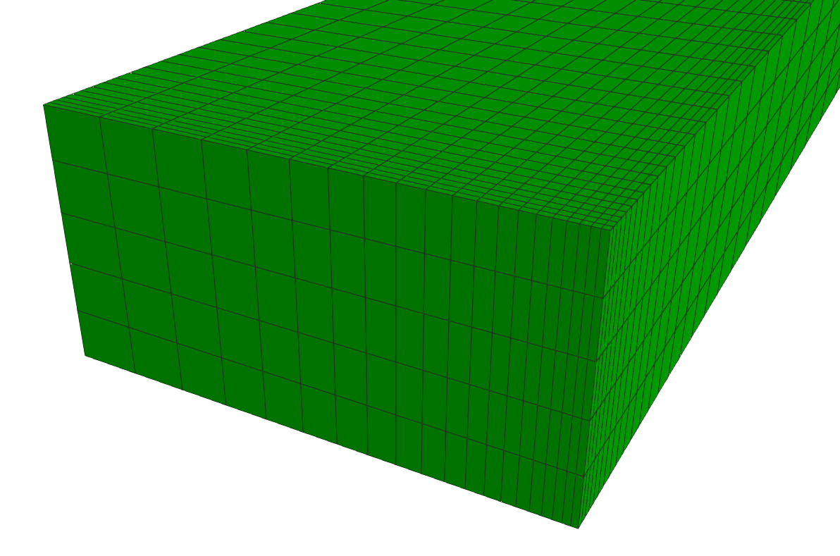
(g) Close up of right corner for 3000 el.

Figure 8: Mesh refinements for symmetric part of clamped tissue stripe.

In the next example we consider the volumetric growth process within a tissue stripe that is clamped at both ends such that no stresses are induced at time $t=0$. Under these conditions, the tissue stripe is expected to shrink, which induces a homeostatic stress state that is dominated by tension. Such effects have been shown experimentally e.g. by Ghazanfari et al. [2015] among others. As illustrated in Figure 7, symmetric properties are exploited such that only a quarter of the full specimen is used for the following simulations. The elastic and growth related material parameters applied in this example are chosen in such a way that the desired shrinkage of the specimen is achieved. These parameters are given in Table 1. For the spatial discretisation, a standard linear (Q1) finite element formulation is adopted with various meshes containing $360$, $408$, $450$, $1000$ and $3000$ elements (see Figure 8). Since the most pronounced stresses are expected to occur in the lower right corner of the symmetric specimen, the mesh is refined with a focus on this particular region.

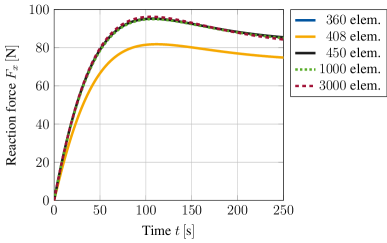
Figure 9: Reaction force of a clamped tissue stripe evaluated at $z=0$ for various mesh sizes. Mesh convergence can be observed nicely.

When considering the reaction force $F_{x}$ evaluated over time at $z=0$, Figure 9 shows good convergence behaviour for increasing number of elements within the mesh. Similar results can be obtained when evaluating the reaction forces in $y$ and $z$ direction, respectively. Although the solution of a mesh containing $450$ elements has already reached convergence, for visualization purposes, the finest discretisation containing $3000$ elements is used in the following.

To show the capabilities of the newly introduced material model, we next compare its response to the growth behaviour of a well established model for isotropic volumetric growth. For this, we adapted the model of Lubarda and Hoger [2002] such that it is capable of reaching a prescribed homeostatic state. Details about the evolution equations for this particular model are given in Appendix A.2. Within this formulation, we use the material parameter $M_{crit}=80~{}\text{MPa}$ to describe the homeostatic stress state that shall ultimately be reached. For the positive and negative growth velocities $k^{+}=0.1$ and $k^{-}=0.1$ are chosen, respectively. The upper and lower growth boundaries are set to $\vartheta^{+}=2.0$ and $\vartheta^{-}=0.25$, while the shape factors are given as $\gamma^{+}=2$ and $\gamma^{-}=3$.

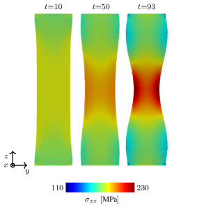
(a) Isotropic growth model using a modified version of Lubarda and Hoger [2002]

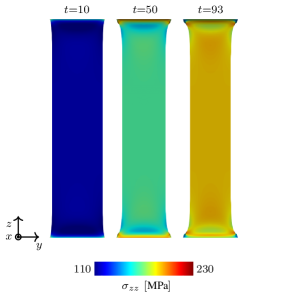
(b) New volumetric growth model using the general growth potential

Figure 10: Comparison of an isotropic growth model with the newly introduced formulation. The response of a clamped tissue stripe differs significantly in both, shape as well as the displayed stress response (Cauchy stresses $\sigma_{zz}$).

First of all it is important to notice that the given isotropic formulation shows severe stability problems for the example at hand. More precisely, as soon as material parameters are chosen such that a similar homeostatic stress state shall be reached within the specimen, the simulation becomes unstable after a finite number of time steps and eventually breaks. When taking a closer look at the evolution of the growth process as it is shown for three distinct time steps in Figure 10, it is obvious that the starting point of the instability can be located at the clamping of the tissue stripe. Due to the initial contraction of the overall tissue stripe, a multi-axial stress state is induced at the clamping. In this region, the stress state soon exceeds the desired homeostatic state which yields an expansion of the material in order to release excessive stresses. Whilst the newly derived growth model reduces this stress state by expanding anisotropically, the isotropic formulation seems not to be able to deal with this effect. This is due to the fact that an isotropic growth formulation can only predict expansion or shrinkage uniformly in all three spatial dimensions. Such a uniform expansion at the foot of the specimen results in a passive compression of the specimens middle part, reducing the overall stress within this region and therefore inducing further contraction. This again triggers an increasing expansion in the foot of the specimen. A vicious cycle is born, which eventually leads to the hourglass like shape of the specimen as it is shown in Figure 10(a). Ultimately, this leads to instabilities and a failing simulation at $t=93$. For sure, it is possible to reduce such unwanted behaviour by variation of the material parameters. Nevertheless, the general problem of a non-physical expansion in the foot area could not be cured with such an approach. This example shows clearly how restrictive and, therefore, unsuitable the assumption of isotropic growth is, even for a relatively simple structure as the one shown in this example. Taking a closer look at the stress response of the newly derived model, one can observe the exceeding maximum principal Cauchy stresses $\sigma_{max}$ located at the clamped foot of the specimen (see Figure 11) being released due to the anisotropic expansion process. This effect can also be observed in Figure 9, where the reaction forces reach a maximum at time $t=100$ and decrease afterwards to approach a converged state. Unfortunately, this effect also leads to a pronounced distortion of the associated elements within the corners of the clamped stripe. Figure 11 shows that this artefact is even noticable for the finest mesh evaluated. Nevertheless, it is important to emphasize that this effect so far does not have an influence on the stability of the given simulation. Due to the incompressible nature of the material, it is possible that such behaviour is also amplified by shear or volumetric locking effects and would not occur in such a pronounced manner if locking would not play a role. However, the influence of possible locking effects is out of scope for this work.

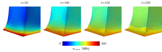
Figure 11: Pronounced distortion of elements at the clamped corner due to growth related reduction of exceeding stresses. Maximum principal Cauchy stresses are plotted for four different snapshots in time.

5 Conclusion and outlook

In this paper, we developed a novel model for the description of stress driven volumetric growth. This approach is based on the well established multiplicative split of the deformation gradient into an elastic and a growth related part. Furthermore, we made the assumption that the given material adapts to its surroundings such that a certain homeostatic stress state is induced within the material. For this homeostatic state, we assume that it can be described in terms of a scalar valued stress like quantity, which led us to the definition of a growth potential. With this idea in hand, we defined an evolution law for the growth related right Cauchy-Green tensor by means of a time dependent associative rule. This approach is similar but not identical to those often used in the field of finite visco-plasticity. With these basic modelling assumptions, we were able to show that this approach is capable of simulating both, isotropic and anisotropic growth behaviour within one singular formulation. The distinction between isotropic and anisotropic response is merely a question of the applied boundary conditions and not a-priori prescribed by the structure of the growth tensor. The advantages of this approach have been shown by comparing it to a standard formulation of isotropic growth. In the authors’ opinion, the results of the evaluations shown within this publication are very promising. Unfortunately, we were not able to validate the given model due to the lack of experimental data published in the literature. Conducting meaningful experiments would therefore be a first step towards validating the model described above. Since the overall framework of the model is quiet general, it seems possible to easily adapt the growth behaviour to fit various experiments. For this, the choice of alternative descriptions for the growth potential as well as the evolution equation for the growth multiplier could be investigated. To this point, our formulation makes use of a purely isotropic elastic ground model, i.e. Neo-Hooke. Since biological tissue by its very own nature is composed of various components, such as e.g. collagen and elastin, the assumption of material isotropy is not ideal. Therefore, we suggest that the given elastic ground model could be extended to also capture the anisotropic nature of the underlying material response properly. This could be achieved by introducing an additional dependency within the Helmholtz free energy that is defined by means of structural tensors describing e.g. the direction of collagen fibres. Furthermore, the investigation of locking effects triggered by the nearly incompressible material behaviour of biological tissues might also be of interest. Since standard low order finite element formulations are particularly vulnerable in this area, the finite element implementation should therefore be considered more closely. Investigating the influence of reduced integration finite elements seems to be of high benefit. Especially the element formulations Q1SP (see Reese [2005]) or Q1STx (see Schwarze and Reese [2011], Barfusz et al. [2021]) could improve the computation in terms of computational accuracy as well as computational speed.

Appendix A Appendix

A.1 Invariants of Mandel stress tensor and Kirchhoff stress tensor

The Kirchhoff stress tensor is defined as

$$\boldsymbol{\tau}=\mathbf{F}\mathbf{S}\mathbf{F}^{T}.$$

Making use of the identity $\mathbf{C}_{e}\mathbf{F}_{g}=\mathbf{F}_{g}^{-T}\mathbf{C}$ and using a push forward operation on the second Piola-Kirchhoff stress tensor $\mathbf{S}$, the definition of the Mandel stress tensor can be rewritten as

$$\begin{split}\mathbf{M}&=\mathbf{C}_{e}\mathbf{F}_{g}\mathbf{S}\mathbf{F}_{g}^{T}\\ &=\mathbf{F}_{g}^{-T}\mathbf{C}\mathbf{S}\mathbf{F}_{g}^{T}.\end{split}$$

With this at hand, it is easy to show that the main invariants $J_{\alpha}$ with $\alpha\in{1,2,3}$ are identical for both, the Mandel and the Kirchhoff stress tensor, i.e.

$$\begin{split}J_{\alpha}&=\operatorname{tr}\left(\mathbf{M}^{\alpha}\right)\\ &=\operatorname{tr}\left(\left(\mathbf{F}_{g}^{-T}\mathbf{C}\mathbf{S}\mathbf{F}_{g}^{T}\right)^{\alpha}\right)\\ &=\operatorname{tr}\left(\left(\mathbf{C}\mathbf{S}\right)^{\alpha}\right)\\ &=\operatorname{tr}\left(\left(\mathbf{F}\mathbf{S}\mathbf{F}^{T}\right)^{\alpha}\right)\\ &=\operatorname{tr}\left(\boldsymbol{\tau}^{\alpha}\right).\end{split}$$

A.2 Isotropic growth model for comparison

The isotropic growth model used for comparison with the anisotropic growth model developed herein is based on the formulation of Lubarda and Hoger [2002]. It uses the multiplicative split of the deformation gradient, i.e.

$$\mathbf{F}=\mathbf{F}_{e}\mathbf{F}_{g},$$

where the growth related deformation gradient is defined as

$$\mathbf{F}_{g}=\vartheta\mathbf{I},$$

with $\vartheta$ describing the growth induced stretch. The evolution equation of this particular model is defined in terms of the Mandel stress tensor $\mathbf{M}$ as well as a set of material parameters, i.e.

$$\dot{\vartheta}:=k(\vartheta)\phi(\mathbf{M}).$$

Here the driving force $\phi$ is defined as

$$\phi:=\operatorname{tr}\mathbf{M}-M_{crit},$$

where $M_{crit}$ describes the desired homeostatic stress state that should be reached by the material. Furthermore, the growth velocity is described by

$$k(\vartheta):=\begin{cases}k^{+}\left(\frac{\vartheta^{+}-\vartheta}{\vartheta^{+}-1}\right)^{\gamma^{+}}&\text{if }\phi>0\\ k^{-}\left(\frac{\vartheta-\vartheta^{-}}{1-\vartheta^{-}}\right)^{\gamma^{-}}&\text{if }\phi<0,\end{cases}$$

with $k^{+}$, $k^{-}$ denote the expansion and contraction speed, respectively. To restrict the growth process, the parameters $\vartheta^{+}$ and $\vartheta^{-}$ are introduced as upper and lower thresholds of the growth induced stretch. Finally, two shape factors for the evolution are described by $\gamma^{+}$ and $\gamma^{-}$. For further information on this particular model, the reader is kindly referred to the original publication.

A.3 Transformation of invariants from intermediate to reference configuration

Reformulating the definition of the referential driving force, i.e.

$$\mathbf{M}-\boldsymbol{\chi}=\mathbf{F}_{g}\mathbf{\Sigma}\mathbf{F}_{g}^{T},$$

directly yields the new definition for the volumetric invariant, i.e.

$$\begin{split}I_{1}&=\operatorname{tr}\left(\mathbf{M}-\boldsymbol{\chi}\right)\\ &=\operatorname{tr}\left(\mathbf{F}_{g}\mathbf{\Sigma}\mathbf{F}_{g}^{T}\right)\\ &=\operatorname{tr}\left(\mathbf{\Sigma}\mathbf{C}_{g}\right).\end{split}$$

Making use of this relation, the deviatoric part of the driving force is given by

$$\begin{split}\operatorname{dev}\left(\mathbf{M}-\boldsymbol{\chi}\right)&=\operatorname{dev}\left(\mathbf{F}_{g}\mathbf{\Sigma}\mathbf{F}_{g}^{T}\right)\\ &=\mathbf{F}_{g}\mathbf{\Sigma}\mathbf{F}_{g}^{T}-\frac{1}{3}\operatorname{tr}\left(\mathbf{F}_{g}\mathbf{\Sigma}\mathbf{F}_{g}^{T}\right)\mathbf{I}\\ &=\mathbf{F}_{g}\mathbf{\Sigma}\mathbf{C}_{g}\mathbf{F}_{g}^{-1}-\frac{1}{3}\operatorname{tr}\left(\mathbf{\Sigma}\mathbf{C}_{g}\right)\mathbf{I}\\ &=\mathbf{F}_{g}\left(\mathbf{\Sigma}\mathbf{C}_{g}-\frac{1}{3}\operatorname{tr}\left(\mathbf{\Sigma}\mathbf{C}_{g}\right)\mathbf{I}\right)\mathbf{F}_{g}^{-1}\\ &=\mathbf{F}_{g}\operatorname{dev}\left(\mathbf{\Sigma}\mathbf{C}_{g}\right)\mathbf{F}_{g}^{-1}.\end{split}$$

Utilizing the properties of the trace operator, the deviatoric invariant can be rewritten as

$$J_{2}=\frac{1}{2}\left(\operatorname{dev}\left(\mathbf{\Sigma}\mathbf{C}_{g}\right)^{2}\right).$$

Appendix B Declarations

B.1 Funding

This work was funded through the grants RE 1057/45-1 (No. 403471716) and RE 1057/46-1 (No. 404502442) of the German Research Foundation (DFG). Furthermore the AiF grant provided under the project number IGF 21348 N/3 was part of funding this work.

B.2 Conflict of interest

The authors of this work certify that they have no affiliations with or involvement in any organization or entity with any financial interest (such as honoraria; educational grants; participation in speakers’ bureaus; membership, employment, consultancies, stock ownership, or other equity interest; and expert testimony or patent-licensing arrangements), or non-financial interest (such as personal or professional relationships, affiliations, knowledge or beliefs) in the subject matter or materials discussed in this manuscript.

B.3 Availability of data and material

The generated data is stored redundantly and will be made available on demand.

B.4 Code availability

The custom routines will be made available on demand. The software package FEAP is a proprietary software and can therefore not be made available.

B.5 Author’s contributions

L. Lamm reviewed the relevant existing literature, performed all simulations, interpreted the results and wrote this article. L. Lamm and H. Holthusen worked out the theoretical material model and impemented it into the finite element software FEAP. H. Holthusen, T. Brepols, S. Jockenhövel and S. Reese gave conceptual advice, contributed in the discussion of the results, read the articel and gave valuable suggestions for improvement. All authors approved the publication of the manuscript.

References

- [1]
- Ahrens et al. [2005] Ahrens, J., Geveci, B. and Law, C. [2005], 36 - paraview: An end-user tool for large-data visualization, in C. D. Hansen and C. R. Johnson, eds, ‘Visualization Handbook’, Butterworth-Heinemann, Burlington, pp. 717 – 731.
- Ambrosi et al. [2019] Ambrosi, D., Ben Amar, M., Cyron, C. J., DeSimone, A., Goriely, A., Humphrey, J. D. and Kuhl, E. [2019], ‘Growth and remodelling of living tissues: perspectives, challenges and opportunities’, Journal of The Royal Society Interface 16(157), 20190233.
- Barfusz et al. [2021] Barfusz, O., Brepols, T., van der Velden, T., Frischkorn, J. and Reese, S. [2021], ‘A single gauss point continuum finite element formulation for gradient-extended damage at large deformations’, Computer Methods in Applied Mechanics and Engineering 373, 113440.
- Bertram [1999] Bertram, A. [1999], ‘An alternative approach to finite plasticity based on material isomorphisms’, International Journal of Plasticity 15(3), 353–374.
- Braeu et al. [2019] Braeu, F., Aydin, R. and Cyron, C. [2019], ‘Anisotropic stiffness and tensional homeostasis induce a natural anisotropy of volumetric growth and remodeling in soft biological tissues’, Biomechanics and Modeling in Mechanobiology 18, 327 – 345.
- Braeu et al. [2017] Braeu, F., Seitz, A., Aydin, R. and Cyron, C. [2017], ‘Homogenized constrained mixture models for anisotropic volumetric growth and remodeling’, Biomechanics and Modeling in Mechanobiology 16, 889 – 906.
- Coleman and Noll [1963] Coleman, B. and Noll, W. [1963], ‘The thermodynamics of elastic materials with heat conduction and viscosity’, Archive for Rational Mechanics and Analysis 13, 167 – 178.
- Cyron et al. [2016] Cyron, C. J., Aydin, R. C. and Humphrey, J. D. [2016], ‘A homogenized constrained mixture (and mechanical analog) model for growth and remodeling of soft tissue’, iomech Model Mechanobiol 15, 1389 – 1403.
- Cyron and Humphrey [2017] Cyron, C. J. and Humphrey, J. D. [2017], ‘Growth and remodeling of load-bearing biological softtissues’, Meccanica 52, 645 – 664.
- de Souza Neto et al. [2008] de Souza Neto, E., Peric, D. and Owen, D. [2008], Computational Methods for Plasticity: Theory and Applications, Wiley, Chichester.
- Dettmer and Reese [2004] Dettmer, W. and Reese, S. [2004], ‘On the theoretical and numerical modelling of armstrong-frederick kinematic hardening in the finite strain regime’, Computer Methods in Applied Mechanics and Engineering 193, 87 – 116.
- Eckart [1948] Eckart, C. [1948], ‘The thermodynamics of irreversible processes. iv. the theory of elasticity and anelasticity’, Phys. Rev. 73, 373–382.
- Fioretta et al. [2019] Fioretta, E., von Boehmer, L., Motta, S., Lintas, V., Hoerstrup, S. and Emmert, M. [2019], ‘Cardiovascular tissue engineering: From basic science to clinical application’, Experimental Gerontology 117, 1 – 12.
- Fung [1995] Fung, Y. [1995], ‘Stress, strain, growth, and remodeling of living organisms’, Theoretical, Experimental, and Numerical Contributions to the Mechanics of Fluids and Solids 46, 469 – 482.
- Gauvin et al. [2013] Gauvin, R., Larouche, D., Marcoux, H., Guignard, R., Auger, F. A. and Germain, L. [2013], ‘Minimal contraction for tissue-engineered skin substitutes when matured at the air–liquid interface’, Journal of Tissue Engineering and Regenerative Medicine 7(6), 452–460.
- Geuzaine and Remacle [2009] Geuzaine, C. and Remacle, J.-F. [2009], ‘Gmsh: a three-dimensional finite element mesh generator with built-in pre- and post-processing facilities’, International Journal For Numerical Methods in Engineering 79, 1309 – 1331.
- Ghazanfari et al. [2015] Ghazanfari, S., Driessen-Mol, A., Strijkers, G., Baaijens, F. and Bouten, C. [2015], ‘The evolution of collagen fiber orientation in engineered cardiovascular tissues visualized by diffusion tensor imaging’, PLoS One 10, 1 – 15.
- Göktepe et al. [2010] Göktepe, S., Abilez, O. and Kuhl, E. [2010], ‘A generic approach towards finite growth with examples of athlete’s heart, cardiac dilation, and cardiac wall thickening’, Journal of the Mechanics and Physics of Solids 58, 1661 – 1680.
- Goriely [2017] Goriely, A. [2017], The Mathematics and Mechanics of Biological Growth, Vol. 45 of Interdisciplinary Applied Mathematics, Springer Nature, New York.
- Himpel et al. [2005] Himpel, G., Kuhl, E., Menzel, A. and Steinmann, P. [2005], ‘Computational modelling of isotropic multiplicative growth’, Computer Modeling in Engineering and Science 8, 1 – 14.
- Humphrey and Rajagopal [2002] Humphrey, J. D. and Rajagopal, K. R. [2002], ‘A constrained mixture model for growth and remodeling of soft tissues’, Mathematical models and methods in applied sciences 12(03), 407–430.
- Korelc [2002] Korelc, J. [2002], ‘Multi-language and multi-environment generation of nonlinear finite element codes’, Engineering with Computers 18, 312 – 327.
- Korelc [2009] Korelc, J. [2009], ‘Automation of primal and sensitivity analysis of transient coupled problems’, Computational Mechanics 44, 631 – 649.
- Korelc and Stupkiewicz [2014] Korelc, J. and Stupkiewicz, S. [2014], ‘Closed-form matrix exponentials and its application to finite-strain plasticity’, Numerical Methods in Engineering 98, 960 – 987.
- Kröner [1959] Kröner, E. [1959], ‘Allgemeine kontinuumstheorie der versetzungen und eigenspannungen’, Arch. Rational Mech. Anal. 4(1), 273 – 334.
- Kuhl and Steinmann [2003] Kuhl, E. and Steinmann, P. [2003], ‘Mass- and volume-specific views on thermodynamics for open systems’, Proceedings of the royal society A 459, 2547 – 2568.
- Lee [1969] Lee, E. H. [1969], ‘Elastic-Plastic Deformation at Finite Strains’, Journal of Applied Mechanics 36(1), 1–6.
- Lubarda and Hoger [2002] Lubarda, V. and Hoger, A. [2002], ‘On the mechanics of solids with a growing mass’, International Journal of Solids and Structures 39, 4627 – 4664.
- Menzel [2005] Menzel, A. [2005], ‘Modelling of anisotropic growth in biological tissues. a new approach and computational aspects’, Biomechanics and Modeling in Mechanobiology 3, 147 – 171.
- Noll [1958] Noll, W. [1958], ‘A mathematical theory of the mechanical behavior of continuous media’, Arch. Rational Mech. Anal. 2, 197 – 226.
- Perzyna [1966] Perzyna, P. [1966], ‘Fundamental problems in viscoplasticity’, Advances in Applied Mechanis 9, 243 – 377.
- Perzyna [1971] Perzyna, P. [1971], ‘Thermodynamic theory of viscoplysticity’, Advances in Applied Mechanis 11, 313 – 354.
- Reese [2005] Reese, S. [2005], ‘On a physically stabilized one point finite element formulation for three-dimensional finite elasto-plasticity’, International Journal for Numerical Methods in Engineering 194, 4685 – 4715.
- Reese et al. [2021] Reese, S., Brepols, T., Fassin, M., Poggenpohl, L. and Wulfinghoff, S. [2021], ‘Using structural tensors for inelastic material modeling in the finite strain regime - a novel approach to anisotropic damage’, Journal of the Mechanics and Physics of Solids 146, 104174.
- Reese and Govindjee [1998] Reese, S. and Govindjee, S. [1998], ‘A theory of finite viscoelasticity and numerical aspects’, International Journal of Solids and Structures 35, 3455 – 3482.
- Rodriguez et al. [1994] Rodriguez, E., Hoger, A. and McCulloch, A. [1994], ‘Stress-dependent finite growth in soft elastic tissues’, Journal of Biomechanics 27, 455 – 467.
- Schwarze and Reese [2011] Schwarze, M. and Reese, S. [2011], ‘A reduced integration solid-shell finite element based on the eas and the ans concept—large deformation problems’, International Journal for Numerical Methods in Engineering 85, 289 – 329.
- Simo [1992] Simo, J. [1992], ‘Algorithms for static and dynamic multiplicative plasticity that preserve the classical return mapping schemes of the infinitesimal theory’, Computer Methods in Applied Mechanics and Engineering 99, 61 – 112.
- Simo and Hughes [1998] Simo, J. and Hughes, T. [1998], Computational Inelasticity, Vol. 7 of Interdisciplinary Applied Mathematics, Springer Nature, New York.
- Skalak [1981] Skalak, R. [1981], Growth as a finite displacement field, in D. E. Carlson and R. T. Shield, eds, ‘Proceedings of the IUTAM Symposium on Finite Elasticity’, Springer Netherlands, Dodrecht, pp. 347 – 355.
- Skalak et al. [1982] Skalak, R., Dasgupta, G., Moss, M., Otten, E., Dullemeijer, P. and Vilmann, H. [1982], ‘Analytical description of growth’, Journal of Theoretical Biology 94(3), 555–577.
- Soleimani et al. [2020] Soleimani, M., Muthyala, N., Marino, M. and Wriggers, P. [2020], ‘A novel stress-induced anisotropic growth model driven by nutri-cent diffusion: theory, fem implementation and applications in bio-mechanical problems’, Journal of the Mechanics and Physics of Solids 144, 104097.
- Stassi-D’Alia [1967] Stassi-D’Alia, F. [1967], ‘Flow and fracture of materials according to a new limiting condtition of yielding’, Meccanica 2, 178 – 195.
- Svendsen [2001] Svendsen, B. [2001], ‘On the modelling of anisotropic elastic and inelastic material behaviour at large deformation’, International Journal of Solids and Structures 38(52), 9579–9599.
- Tange [2011] Tange, O. [2011], ‘Gnu parallel: The command-line power tool’, ;login: 36(1), 42 – 47.
- Taylor and Govindjee [2020] Taylor, R. and Govindjee, S. [2020], FEAP - - A Finite Element Analysis Program, University of California at Berkeley, http://projects.ce.berkeley.edu/feap/manual_86.pdf. [Online; accessed 19-January-2021].
- Tschoegl [1971] Tschoegl, N. [1971], ‘Failure surfaces in principal stress space’, Journal of Polymer Science Part C: Polymer Symposia 32, 239 – 267.
- Vladimirov et al. [2008] Vladimirov, I., Pietryga, M. and Reese, S. [2008], ‘On the modelling of non-linear kinematic hardening at finite strains with application to springback - comparison of time integration algorithms’, Numerical Methods in Engineering 75, 1 – 28.
- Weber and Anand [1990] Weber, G. and Anand, L. [1990], ‘Finite deformation constitutive equations and a time integration procedure for isotropic, hyperelastic - viscoplastic solids’, Computer Methods in Applied Mechanics and Engineering 79, 173 – 202.