Typical absolute continuity for classes of dynamically defined measures

Abstract.

We consider one-parameter families of smooth uniformly contractive iterated function systems $\{f^{\lambda}_{j}\}$ on the real line. Given a family of parameter dependent measures $\{\mu_{\lambda}\}$ on the symbolic space, we study geometric and dimensional properties of their images under the natural projection maps $\Pi^{\lambda}$. The main novelty of our work is that the measures $\mu_{\lambda}$ depend on the parameter, whereas up till now it has been usually assumed that the measure on the symbolic space is fixed and the parameter dependence comes only from the natural projection. This is especially the case in the question of absolute continuity of the projected measure $(\Pi^{\lambda})_{*}\mu_{\lambda}$, where we had to develop a new approach in place of earlier attempt which contains an error. Our main result states that if $\mu_{\lambda}$ are Gibbs measures for a family of Hölder continuous potentials $\phi^{\lambda}$, with Hölder continuous dependence on $\lambda$ and $\{\Pi^{\lambda}\}$ satisfy the transversality condition, then the projected measure $(\Pi^{\lambda})_{*}\mu_{\lambda}$ is absolutely continuous for Lebesgue a.e. $\lambda$, such that the ratio of entropy over the Lyapunov exponent is strictly greater than $1$. We deduce it from a more general almost sure lower bound on the Sobolev dimension for families of measures with regular enough dependence on the parameter. Under less restrictive assumptions, we also obtain an almost sure formula for the Hausdorff dimension. As applications of our results, we study stationary measures for iterated function systems with place-dependent probabilities (place-dependent Bernoulli convolutions and the Blackwell measure for binary channel) and equilibrium measures for hyperbolic IFS with overlaps (in particular: natural measures for non-homogeneous self-similar IFS and certain systems corresponding to random continued fractions).

1. Introduction

Let ${\mathcal{A}}=\{1,\ldots,m\}$ and let $\Psi=\{f_{j}\}_{j\in{\mathcal{A}}}$ be a set of contracting smooth functions on a compact interval $I\subset\mathbb{R}$ mapping $I$ into itself. We call the set $\Psi$ an iterated function system (IFS) on $I$. It is well known that there exists a unique non-empty compact set $\Lambda\subseteq I$ such that it is invariant with respect to the IFS, that is $\Lambda=\bigcup_{j\in{\mathcal{A}}}f_{j}\left(\Lambda\right)$. We call the set $\Lambda$ the attractor of the IFS, see Hutchinson [17] or Falconer [11].

Moreover, let $\Omega={\mathcal{A}}^{\mathbb{N}}$ be the symbolic space and $\sigma$ the left shift transformation on $\Omega$. There is a natural projection $\Pi\colon\Omega\mapsto\Lambda$ defined as

$$\Pi(\omega):=\lim_{n\rightarrow\infty}f_{\omega_{1}}\circ\cdots\circ f_{\omega_{n}}(x),\text{ for $\omega=(\omega_{1},\omega_{2},\ldots)\in\Omega$,}$$

where $x\in I$ is any point (the limit does not depend on the choice of $x$). If $\mu$ is a probability measure on $\Omega$ then we call the measure $\Pi_{*}\mu=\mu\circ\Pi^{-1}$ on $\Lambda$ the push-forward measure of $\mu$. Usually, we assume that $\mu$ is $\sigma$-invariant and ergodic. Let us denote the entropy of $\mu$ by $h_{\mu}$ and the Lyapunov exponent by $\chi_{\mu}$. The ratio $h_{\mu}/\chi_{\mu}$ is called the Lyapunov dimension of $\mu$.

Considerable attention has been paid to the dimension theory and measure theoretic properties of attractors and push-forward measures of iterated function systems. A natural upper bound for the Hausdorff and box counting dimension of the attractor is the unique root $s$ of the pressure function $s\mapsto P(-s\log|f^{\prime}_{\omega_{1}}(\Pi(\sigma\omega))|)=0$, see the next section for definitions. Ruelle [36] showed that in case of separation, e.g., the Open Set Condition (OSC), the Hausdorff dimension of the attractor equals to the root of the pressure function, see also Falconer [10]. Similarly, the Hausdorff dimension of the push-forward measures is bounded above by the Lyapunov dimension of $\mu$; moreover, if the OSC holds, then the dimension equals to the Lyapunov dimension of $\mu$, see Feng and Hu [13].

The situation becomes more complicated if there are overlaps between the maps. To handle this case, Pollicott and Simon [34] introduced the transversality method for parametrized families of iterated function systems. Later, this method was widely applied and generalised, see for example, Solomyak [45, 46], Peres and Solomyak [30, 31], Simon and Solomyak [42], Neunhäuserer [26], Ngai and Wang [27], and Peres and Schlag [29].

We have a deeper understanding in the special case, when the maps of the IFS are similarities and the measure $\mu$ is Bernoulli, thanks to recent results. In his seminal paper, Hochman [15], using methods of additive combinatorics, determined the value of the Hausdorff dimension of the attractor (self-similar set) and the push-forward measure (self-similar measure) under the exponential separation condition. Relying on this result and the Fourier decay of the push-forward measure, Shmerkin [39] proved that the exceptional set of parameters for absolute continuity of Bernoulli convolution measures has zero Hausdorff dimension. These results were extended by Shmerkin and Solomyak [40] and Saglietti, Shmerkin and Solomyak [37] to more general IFS of similarities and Bernoulli measures. Further progress on absolute continuity of Bernoulli convolutions was obtained by Varjú [48]. Jordan and Rapaport [19] showed that the dimension of the push-forward measure of any ergodic shift-invariant measure equals to the entropy over Lyapunov exponent ratio under the exponential separation condition. However, such strong results are unknown in the case when the IFS consists of general conformal maps.

Simon, Solomyak and Urbański [43, 44] showed that if a smoothly parametrized (hyperbolic or parabolic) family of conformal IFS’s $\{f_{i}^{\lambda}\}_{i\in{\mathcal{A}}}$ satisfies the transversality condition over a bounded open domain $U$ of parameters, then for Lebesgue almost every parameter $\lambda\in U$ the dimension of the attractor equals to $\min\{1,s_{\lambda}\}$, where $s_{\lambda}$ is the root of the pressure function, which depends on the parameter. Moreover, it has positive Lebesgue measure for almost every parameter, such that $s_{\lambda}>1$. Similarly, the dimension of the push-forward measure of any fixed ergodic shift-invariant measure $\mu$ is equal to the Lyapunov dimension of $\mu$, and the measure is absolutely continuous for almost every parameter where $h_{\mu}/\chi_{\mu}>1$. Peres and Schlag [29] obtained upper bounds on the Hausdorff dimension of the set of exceptional parameters using a version of transversality, in the framework of a “generalized projection”. All these results required a fixed ergodic shift-invariant measure on $\Omega$. However, there are important cases when the measure on $\Omega$ depends also on the parameter $\lambda$. There are two natural occurrences of such situation.

One is the so-called place-dependent measures, which were studied by Fan and Lau [12], Hu, Lau and Wang [16], Jaroszewska [18], Jaroszewska and Rams [19], Kwiecińska and W. Słomczyński [22], Czudek [8] and others. Let $\{p_{i}\}_{i\in{\mathcal{A}}}$ be a family of Hölder continuous maps $p_{i}\colon I\mapsto[0,1]$ such that $\sum_{i\in{\mathcal{A}}}p_{i}\equiv 1$. Fan and Lau [12] showed that there exists a unique measure $\nu$ on $I$ such that

$$\int\varphi(x)d\nu(x)=\int\sum_{i\in{\mathcal{A}}}p_{i}(x)\varphi(f_{i}(x))d\nu(x)\ \ \text{ for any continuous test function }\varphi.$$

In view of a result by Bowen [6], it is clear that $\nu$ is the push-forward of the equilibrium measure $\mu$ (on the symbolic space ${\mathcal{A}}^{\mathbb{N}}$) of the pressure corresponding to the potential $\omega\mapsto\log p_{\omega_{1}}(\Pi(\sigma\omega))$. It is shown in [12] that if the open set condition holds, then the dimension of $\nu$ equals $\frac{h_{\mu}}{\chi_{\mu}}$. In the case of parametrized family $\{f_{i}^{\lambda}\}_{i\in{\mathcal{A}}}$ the equilibrium measure depends on the parameter.

Bárány [1] studied such parametrized place-dependent families and claimed to generalise the result of [44] for this case. However, the proof contains a crucial error, which cannot be fixed easily. In the present paper we have managed to overcome the obstacles and correct the error, using a delicate modification of the Peres-Schlag [29] method. In fact, our results are much more general. Here we state the main result in the most important situation, in non-technical terms; complete statements may be found in Section 3.

Theorem 1.1.

Let $\{f_{j}^{\lambda}\}_{j\in{\mathcal{A}}}$ be a $C^{2+\delta}$ smooth family of hyperbolic IFS on a compact interval, smoothly depending on a real parameter $\lambda\in U$, and let $\Pi^{\lambda}:\Omega\to\mathbb{R}$ be the corresponding natural projection map. We assume that the (classical) transversality condition holds on $U$. Let $\{\mu_{\lambda}\}_{\lambda\in U}$ be a family of Gibbs measures, corresponding to a family of Hölder-continuous potentials, with a Hölder-continuous dependence on parameter. Then the push-forward measure $(\Pi^{\lambda})_{*}\mu_{\lambda}$ is absolutely continuous for Lebesgue-a.e. $\lambda\in U$ such that $h_{\mu_{\lambda}}/\chi_{\mu_{\lambda}}>1$.

We also showed, under slightly less restrictive assumptions, that the push-forward measure $(\Pi^{\lambda})_{*}\mu_{\lambda}$ has Hausdorff dimension equal to $\min\{1,h_{\mu_{\lambda}}/\chi_{\mu_{\lambda}}\}$ almost everywhere in $U$. The proof of this result is not as difficult, similar to Bárány-Rams [7], and is included for completeness.

Place-dependent measures play an important role, for example, in the theory of hidden Markov chains. Blackwell [5] expressed the entropy of hidden Markov chains over finite state space as an integral with respect to a place-dependent measure, which is nowadays called the Blackwell measure. The singularity of the Blackwell measure was studied by Bárány, Pollicott and Simon [3]. Later, Bárány and Kolossváry [2] showed that the transversality condition holds on a certain region of parameters and applied the main theorem of Bárány [1] to claim absolute continuity almost everywhere in this region. Since the Blackwell measure satisfies the assumptions of the main result of the present paper, we recover this result of Bárány and Kolossváry [2].

Another important case, when the parameter dependence of the measure occurs, is the natural measure of the parametrized IFS $\{f_{i}^{\lambda}\}_{i\in{\mathcal{A}}}$, which is the equilibrium measure $\nu_{\lambda}$ with respect to the potential $\omega\mapsto s_{\lambda}\log|(f_{\omega_{1}}^{\lambda})^{\prime}(\Pi_{\lambda}(\sigma\omega))|$. See [35] for more on the subject. In case of overlaps, neither the dimension nor the absolute continuity was known. Our result applies in this situation as well. In particular, it follows that a natural measure for non-homogeneous self-similar IFS is absolutely continuous for almost every parameter with similarity dimension strictly larger than $1$, in the transversality region (such regions were found e.g. for non-homogeneous Bernoulli convolutions, see [26, 27]). A similar conclusion is obtained for a (non-linear) system corresponding to certain random continued fractions.

1.1. About the proof

In order to prove “almost-sure” results for push-forwards of measures $\mu_{\lambda}$ depending on parameter, we need to impose “correct” continuity assumptions on the measure, which are, on one hand, sufficiently strong to apply the techniques, but on the other hand, can be verified in practice. These continuity assumptions are imposed on measures of cylinder sets and involve estimates of the ratios $\mu_{\lambda}([w])/\mu_{\lambda_{0}}([w])$ for $\lambda$ close to $\lambda_{0}$. For the result on Hausdorff dimension of the push-forward measure, the condition is less restrictive, see (M0) below, and we could apply more or less “classical” transversality techniques, since roughly speaking, we can “afford” to lose $\epsilon$ in dimension estimates.

The results on absolute continuity are much more delicate. The idea is to adapt the method of Peres-Schlag [29] and to show that almost everywhere in the super-critical parameter interval, the Sobolev dimension of the push-forward measure is greater than one. This implies not just absolute continuity, but also $L^{2}$-density and even existence of $L^{2}$-fractional derivatives of some positive order. This adaptation is not straightforward. First, [29] uses the notion of transversality of degree $\beta$, which has to be verified in our situation. Second, we cannot apply the result of [29] as a “black box”, but rather have to work at a certain “discretized” level, in order to utilize the continuity assumptions on the measure dependence, see (M) below. It should be mentioned that Peres-Schlag [29] used their theorem on Sobolev dimension to estimate the Hausdorff dimension of the set of exceptional parameters for absolute continuity. We do not deal with this issue and only concern ourselves with almost sure absolute continuity. We should also point out that [29] contains two kinds of results: the infinite regularity case and the limited regularity case. It is the latter one (in fact, with the lowest possible regularity) that we adapt.

Another issue that comes up is that absolute continuity by the Peres-Schlag method is originally shown under the assumption that the correlation dimension of the measure $\mu_{\lambda}$ is greater than one (in the metric corresponding to $\lambda$), which is a stronger condition, in general, than $h_{\mu_{\lambda}}/\chi_{\mu_{\lambda}}>1$. The usual approach to overcome this is to restrict the measure to a “Egorov set”, where the convergence in the definitions of the entropy and the Lyapunov exponent is uniform. This works fine when we consider the push-forward of a fixed measure, but in our case this is more delicate, since we have to guarantee that (M) is preserved under the restriction. Here we manage to overcome the obstacle with the help of large deviations estimates for Gibbs measures (see [49, 9, 28]).

1.2. Organization of the paper

In the next section we collect all the main assumptions, definitions and notation. In Section 3 we state our main results. In fact, we state two results on almost sure absolute continuity: in the first one we don’t make the assumption that $\mu_{\lambda}$ is a family of Gibbs measure and only assume what is needed to prove almost sure absolute continuity in the parameter interval where the correlation dimension is greater than one. The second one is the sharp result for Gibbs measures. Section 4 is devoted to preliminaries, mainly the regularity properties of the IFS and the parameter dependence. Shorter proofs are included in this section, but longer and more technical calculations are postponed to the Appendices. In Section 5 we prove the theorem on the Hausdorff dimension of the push-forward measures. In Section 6 we verify that the transversality of degree $\beta$ condition of Peres-Schlag holds under our “standard” transversality assumptions, given sufficient regularity. The “heart” of the proof, namely, the adaptation of a discretized Peres-Schlag method, where transversality condition is used, is contained in Section 7. Section 8 is devoted to the case of Gibbs measures: first we show that under the continuity assumptions on the potential, the Gibbs measures satisfy (M), and then use large deviation estimates to extract “large submeasures” still satisfying (M), but with correlation dimension arbitrary close to $h_{\mu_{\lambda}}/\chi_{\mu_{\lambda}}$. After that, it only remains to collect the pieces to complete the proof of the main results; this is done in Section 9. Section 10 is devoted to applications. There we also present a sufficient condition for transversality to hold for "vertical" translation families of the form $f^{\lambda}_{j}(x)=f_{j}(x)+a_{j}(\lambda)$. Last, but not least, Section 11 contains some open questions and possible directions for further research.

1.3. Acknowledgements

Balázs Bárány and Károly Simon acknowledge support from grants OTKA K123782 and OTKA FK134251. Boris Solomyak and Adam Śpiewak acknowledge support from the Israel Science Foundation, grant 911/19.

2. Assumptions, notation and definitions

Let ${\mathcal{A}}=\{1,\ldots,m\}$ and suppose we have an IFS $\{f_{j}^{\lambda}\}_{j\in{\mathcal{A}}}$ on a compact interval $X\subset\mathbb{R}$, depending on a parameter $\lambda\in\overline{U}\subset\mathbb{R}$ with $U$ being an open and bounded interval. Let ${\rm diam}(X)=1$ for simplicity. We assume that there exists $\delta\in(0,1]$ such that

1. the maps $f_{j}^{\lambda}$ are $C^{2+\delta}$-smooth on $X$ with $M_{1}=\sup\limits_{\lambda\in U}\sup\limits_{j\in{\mathcal{A}}}\left\{\left\|\frac{d^{2}}{dx^{2}}f^{\lambda}_{j}\right\|_{\infty}\right\}<\infty$ and there exist constants $C_{1},C_{2}>0$ such that

   $$\left|\frac{d^{2}}{dx^{2}}f^{\lambda}_{j}(x)-\frac{d^{2}}{dx^{2}}f^{\lambda}_{j}(y)\right|\leq C_{1}|x-y|^{\delta}\text{ and }\left|\frac{d^{2}}{dx^{2}}f^{\lambda_{1}}_{j}(x)-\frac{d^{2}}{dx^{2}}f^{\lambda_{2}}_{j}(x)\right|\leq C_{2}|\lambda_{1}-\lambda_{2}|^{\delta}$$

   hold for all $x,y\in X,\ j\in{\mathcal{A}},\ \lambda,\lambda_{1},\lambda_{2}\in U$.

   
   

2. the maps $\lambda\mapsto f^{\lambda}_{j}(x)$ are $C^{1+\delta}$-smooth on $U$ and there exists a constant $C_{3}>0$ such that

   $$\left|\frac{d}{d\lambda}f_{j}^{\lambda_{1}}(x)-\frac{d}{d\lambda}f_{j}^{\lambda_{2}}(x)\right|\leq C_{3}|\lambda_{1}-\lambda_{2}|^{\delta}$$

   holds for all $x\in X,\ j\in{\mathcal{A}},\ \lambda_{1},\lambda_{2}\in U$.

   
   

3. the second partial derivatives $\frac{d^{2}}{dxd\lambda}f^{\lambda}_{j}(x),\frac{d^{2}}{d\lambda dx}f^{\lambda}_{j}(x)$ exist and are continuous on $U\times X$ (hence equal) with $M_{2}=\sup\limits_{j\in{\mathcal{A}}}\sup\limits_{\lambda\in U}\left\|\frac{d^{2}}{d\lambda dx}f^{\lambda}_{j}(x)\right\|_{\infty}<\infty$ and there exist constants $C_{4},C_{5}>0$ such that

   $$\left|\frac{d^{2}}{dxd\lambda}f^{\lambda}_{j}(x)-\frac{d^{2}}{dxd\lambda}f^{\lambda}_{j}(y)\right|\leq C_{4}|x-y|^{\delta}\text{ and }\left|\frac{d^{2}}{dxd\lambda}f^{\lambda_{1}}_{j}(x)-\frac{d^{2}}{dxd\lambda}f^{\lambda_{2}}_{j}(x)\right|\leq C_{5}|\lambda_{1}-\lambda_{2}|^{\delta}$$

   hold for all $x,y\in X,\ j\in{\mathcal{A}},\ \lambda,\lambda_{1},\lambda_{2}\in U$.

   
   

4. the system $\{f_{j}^{\lambda}\}_{j\in{\mathcal{A}}}$ is uniformly hyperbolic and contractive: there exists $\gamma_{1},\ \gamma_{2}>0$ such that

   $$0<\gamma_{1}\leq|(\textstyle{\frac{d}{dx}}f_{j}^{\lambda})(x)|\leq\gamma_{2}<1\ \ \mbox{holds for all}\ j\in{\mathcal{A}},\ x\in X,\ \lambda\in\overline{U}.$$

Let $\Omega={\mathcal{A}}^{\mathbb{N}}$ and let $\sigma$ denote the left shift on $\Omega$. Let $\Omega^{*}=\bigcup\limits_{n\geq 0}{\mathcal{A}}^{n}$ be the set of finite words over ${\mathcal{A}}$ and let $|u|$ be the length of $u$. For $u=(u_{1},\ldots u_{n})\in\Omega^{*}$ denote

$$f^{\lambda}_{u}=f^{\lambda}_{u_{1}\ldots u_{n}}:=f^{\lambda}_{u_{1}}\circ\ldots\circ f^{\lambda}_{u_{n}}$$

(with $f_{u}=\mathrm{id}$ if $u$ is an empty word) and let $\Pi^{\lambda}:\Omega\to X,\ \lambda\in\overline{U}$

$$\Pi^{\lambda}(u)=\lim_{n\to\infty}f^{\lambda}_{u_{1}\ldots u_{n}}(x_{0})\text{ for }u\in\Omega$$

be the natural projection (it does not depend on the choice of $x_{0}\in X$). For $u\in\Omega^{*}\cup\Omega$ let $u|_{n}=(u_{1},\ldots,u_{n})$ denote the restriction of $u$ to the first $n$ coordinates. For $u=(u_{1},\ldots,u_{n})\in\Omega^{*}$ and $0\leq k\leq|u|$ let $\sigma^{k}u=(u_{k+1},\ldots,u_{n})$. For $u,v\in\Omega$ let $u\wedge v=(u_{1},\ldots,u_{n})$, where $n=\sup\{k\geq 1:u_{k}=v_{k}\}$, i.e. $u\wedge v$ is the common prefix of $u$ and $v$. For $u\in\Omega^{*}$ let $[u]=\{\omega\in\Omega:\omega|_{|u|}=u\}$ be the cylinder corresponding to $u$.

We will assume that the following transversality condition is satisfied for $\lambda\in U$:

1. $\exists\,\eta>0:\ \forall\,u,v\in\Omega,\ \ u_{1}\neq v_{1},\ \left|\Pi^{\lambda}(u)-\Pi^{\lambda}(v)\right|<\eta\implies\left|\textstyle{\frac{d}{d\lambda}}(\Pi^{\lambda}(u)-\Pi^{\lambda}(v))\right|\geq\eta.$

In our setting, transversality condition (T) is equivalent to other transversality conditions appearing in the literature - see Section 10.6 and Lemma 10.7 for details.

Let $\left\{\mu_{\lambda}\right\}_{\lambda\in\overline{U}}$ be a collection of finite Borel measures on $\Omega$. We will consider two continuity assumptions on $\mu_{\lambda}$:

1. for every $\lambda_{0}$ and every $\varepsilon>0$ there exist $C,\xi>0$ such that

   $$C^{-1}e^{-\varepsilon|\omega|}\mu_{\lambda_{0}}([\omega])\leq\mu_{\lambda}([\omega])\leq Ce^{\varepsilon|\omega|}\mu_{\lambda_{0}}([\omega])$$

   holds for every $\omega\in\Omega^{*},\ |\omega|\geq 1$ and $\lambda\in\overline{U}$ with $|\lambda-\lambda_{0}|<\xi$;

1. there exists $c>0$ and $\theta\in(0,1]$ such that for all $\omega\in\Omega^{*},\ |\omega|\geq 1$, and all $\lambda,\lambda^{\prime}\in\overline{U}$,

   $$e^{-c|\lambda-\lambda^{\prime}|^{\theta}|\omega|}\mu_{\lambda^{\prime}}([\omega])\leq\mu_{\lambda}([\omega])\leq e^{c|\lambda-\lambda^{\prime}|^{\theta}|\omega|}\mu_{\lambda^{\prime}}([\omega]).$$

Note that (M) implies (M0).

For a compact metric space $(X,d)$, let $\mathcal{M}(X)$ denote the set of finite Borel measures on $X$ and $\mathcal{P}(X)$ the set of Borel probability measures on $X$. For $\mu\in\mathcal{M}(X)$ and $\alpha>0$, define the $\alpha$-energy as

(2.1) $${\mathcal{E}}_{\alpha}(\mu,d)=\int\int d(x,y)^{-\alpha}d\mu(x)d\mu(y).$$

Define the correlation dimension of $\mu$ with respect to the metric $d$ as

$$\dim_{cor}(\mu,d)=\sup\{\alpha>0:{\mathcal{E}}_{\alpha}(\mu,d)<\infty\}.$$

For a Borel measure $\nu$ on $\mathbb{R}$, the Fourier transform of $\nu$ is given by $\hat{\nu}(\xi)=\int e^{i\xi x}d\nu(x).$ For a finite Borel measure $\nu$ and $\gamma\in\mathbb{R}$, we define the homogenous Sobolev norm as

$$\|\nu\|^{2}_{2,\gamma}=\int\limits_{\mathbb{R}}|\hat{\nu}(\xi)|^{2}|\xi|^{2\gamma}d\xi$$

and the Sobolev dimension

$$\dim_{S}(\nu)=\sup\left\{\alpha\in\mathbb{R}:\int\limits_{\mathbb{R}}|\hat{\nu}(\xi)|^{2}(1+|\xi|)^{\alpha-1}d\xi<\infty\right\}.$$

Note that $0\leq\dim_{S}(\nu)\leq\infty$ and

$$\int\limits_{\mathbb{R}}|\hat{\nu}(\xi)|^{2}(1+|\xi|)^{\alpha-1}d\xi<\infty\ {\iff}\ \int\limits_{\mathbb{R}}|\hat{\nu}(\xi)|^{2}|\xi|^{\alpha-1}d\xi=\|\nu\|_{2,\frac{\alpha-1}{2}}^{2}<\infty$$

for $\alpha>0$ (see [24, Section 5.2]). If $0<\dim_{S}(\nu)<1$, then $\dim_{S}(\nu)=\dim_{cor}(\nu)$, where the correlation dimension is taken with respect to the standard metric on $\mathbb{R}$. If $\dim_{S}(\nu)>1$, then $\nu$ is absolutely continuous with a density (Radon-Nikodym derivative) in $L^{2}(\mathbb{R})$, and moreover $\nu$ has fractional derivatives in $L^{2}$ of some positive order – see [24, Theorem 5.4]

For an IFS $\{f_{j}^{\lambda}\}_{j\in{\mathcal{A}}}$ and a family of shift-invariant and ergodic probability measure $\mu_{\lambda}$ on $\Omega$, let $h_{\mu_{\lambda}}$ be the entropy of $\mu_{\lambda}$ defined as

$$h_{\mu_{\lambda}}=-\lim\limits_{n\to\infty}\frac{1}{n}\sum\limits_{\omega\in{\mathcal{A}}^{n}}\mu_{\lambda}([\omega])\log\mu_{\lambda}([\omega])$$

and let $\chi_{\mu_{\lambda}}$ be the Lyapunov exponent of $\mu_{\lambda}$ given by

$$\chi_{\mu_{\lambda}}=-\int\limits_{\Omega}\log\left|\left(f^{\lambda}_{\omega_{1}}\right)^{\prime}(\Pi^{\lambda}(\sigma\omega))\right|d\mu_{\lambda}(\omega).$$

For $\lambda\in\overline{U}$ we define a metric $d_{\lambda}$ on $\Omega$ by

(2.2) $$d_{\lambda}(u,v)=\left|f_{u\wedge v}^{\lambda}(X)\right|\text{ for }u,v\in\Omega.$$

Let $\phi:\Omega\to\mathbb{R}$ be a continuous function on the symbolic space $\Omega$. A shift-invariant ergodic probability measure $\mu$ on $\Omega$ is called a Gibbs measure of the potential $\phi$ if there exists $P\in\mathbb{R}$ and $C_{G}\geq 1$ such that for every $\omega\in\Omega$ and $n\in{\mathbb{N}}$, holds the inequality

$$C_{G}^{-1}\leq\frac{\mu([\omega|_{n}])}{\exp(-Pn+\sum\limits_{k=0}^{n-1}\phi(\sigma^{k}\omega))}\leq C_{G}.$$

It is known that if $\phi$ is Hölder continuous, then there exists a unique Gibbs measure of $\phi$ (see [6]).

3. Main results

Theorem 3.1.

Let $\{f_{j}^{\lambda}\}_{j\in{\mathcal{A}}}$ be a parametrized IFS satisfying smoothness assumptions (A1) - (A4) and the transversality condition (T) on $U$. Let $\left\{\mu_{\lambda}\right\}_{\lambda\in\overline{U}}$ be a collection of finite ergodic shift-invariant Borel measures on $\Omega$ satisfying (M0), such that $h_{\mu_{\lambda}}$ and $\chi_{\mu_{\lambda}}$ are continuous in $\lambda$. Then equality

$$\dim_{H}((\Pi^{\lambda})_{*}\mu_{\lambda})=\min\left\{1,\frac{h_{\mu_{\lambda}}}{\chi_{\mu_{\lambda}}}\right\}$$

holds for Lebesgue almost every $\lambda\in U$.

The most general version of our main result is the following:

Theorem 3.2.

Let $\{f_{j}^{\lambda}\}_{j\in{\mathcal{A}}}$ be a parametrized IFS satisfying smoothness assumptions (A1) - (A4) and the transversality condition (T) on $U$. Let $\left\{\mu_{\lambda}\right\}_{\lambda\in\overline{U}}$ be a collection of finite Borel measures on $\Omega$ satisfying (M). Then

$$\dim_{S}((\Pi^{\lambda})_{*}\mu_{\lambda})\geq\min\left\{\dim_{cor}(\mu_{\lambda},d_{\lambda}),1+\min\{\delta,\theta\}\right\}$$

holds for Lebesgue almost every $\lambda\in U$, where $d_{\lambda}$ is the metric on $\Omega$ defined in (2.2) and $\delta,\theta$ are from assumptions (A1)-(A4) and (M) respectively. Consequently, $(\Pi^{\lambda})_{*}\mu_{\lambda}$ is absolutely continuous with a density in $L^{2}$ for Lebesgue almost every $\lambda$ in the set $\{\lambda\in U:\dim_{cor}(\mu_{\lambda},d_{\lambda})>1\}$.

In the special case of Gibbs measures for potentials with Hölder continuous dependence on the parameter, we get the following:

Theorem 3.3.

Let $\{f_{j}^{\lambda}\}_{j\in{\mathcal{A}}}$ be a parametrized IFS satisfying smoothness assumptions (A1) - (A4) and the transversality condition (T) on $U$. Let $\left\{\mu_{\lambda}\right\}_{\lambda\in\overline{U}}$ be a family of Gibbs measures on $\Omega$ corresponding to a family of continuous potentials $\phi^{\lambda}\colon\Omega\mapsto\mathbb{R}$ such that there exists $0<\alpha<1$ and $b>0$ with

(3.1) $$\sup_{\lambda\in\overline{U}}\mathrm{var}_{k}(\phi^{\lambda})\leq b\alpha^{k},$$

where $\mathrm{var}_{k}(\phi)=\sup\{|\phi(\omega_{1})-\phi(\omega_{2})|:|\omega_{1}\wedge\omega_{2}|=k\}$. Moreover, suppose that there exist constants $c_{0}>0$ and $\theta>0$ such that

(3.2) $$|\phi^{\lambda}(\omega)-\phi^{\lambda^{\prime}}(\omega)|\leq c_{0}|\lambda-\lambda^{\prime}|^{\theta}\text{ for every $\omega\in\Omega$ and $\lambda,\lambda^{\prime}\in\overline{U}$.}$$

Then $\{\mu_{\lambda}\}_{\lambda\in\overline{U}}$ satisfies (M), hence conclusions of Theorem 3.2 hold (with $\theta$ as in (3.2)). Furthermore, $(\Pi^{\lambda})_{*}\mu_{\lambda}$ is absolutely continuous for Lebesgue almost every $\lambda$ in the set $\{\lambda\in U:\frac{h_{\mu_{\lambda}}}{\chi_{\mu_{\lambda}}}>1\}$.

4. Preliminaries

Throughout this section we assume that we are given an IFS $\{f_{j}^{\lambda}\}_{j\in{\mathcal{A}}}$ satisfying (A1) - (A4) for some $\delta\in(0,1]$. We state several auxiliary results concerning regularity properties of the IFS $\{f_{j}^{\lambda}\}_{j\in{\mathcal{A}}}$ and the natural projection $\Pi^{\lambda}$, which will be used in subsequent sections. As some of the proofs are lengthy, yet standard in techniques, we postpone them partially to the Appendix.

Lemma 4.1.

There exist constants $C_{51}>0$ and $C_{52}>0$ such that

(4.1) $$\left|\frac{d^{2}}{dx^{2}}f^{\lambda}_{u}(x)\right|\leq C_{51}\left|\frac{d}{dx}f^{\lambda}_{u}(x)\right|$$

and

(4.2) $$\left|\frac{d^{2}}{d\lambda dx}f^{\lambda}_{u}(x)\right|\leq C_{52}|u|\left|\frac{d}{dx}f^{\lambda}_{u}(x)\right|$$

hold for all $\lambda\in U,\ x\in X,\ u\in\Omega^{*}$.

Proof.

See Appendix A. ∎

Lemma 4.2 (Parametric bounded distortion property).

There exist constants $c_{62}>0,\ C_{62}>1$ such that inequality

(4.3) $$\frac{1}{C_{62}}e^{-c_{62}|\lambda_{1}-\lambda_{2}||u|}\leq\frac{\left|\frac{d}{dx}f^{\lambda_{1}}_{u}(x)\right|}{\left|\frac{d}{dx}f^{\lambda_{2}}_{u}(y)\right|}\leq C_{62}e^{c_{62}|\lambda_{1}-\lambda_{2}||u|}$$

holds for all $\lambda_{1},\lambda_{2}\in\overline{U},\ x,y\in X,\ u\in\Omega^{*}$.

Proof.

First, let us prove the inequality with $\lambda_{1}=\lambda_{2}$. For $u=(u_{1},\ldots,u_{n})\in\Omega^{*}$, applying (A1) and (A4), together with inequality $\log\frac{x}{y}\leq\frac{\left|x-y\right|}{\min\{x,y\}}$ for $x,y>0$ yields

(4.4) $$\log\frac{\left|\frac{d}{dx}f^{\lambda}_{u}(x)\right|}{\left|\frac{d}{dx}f^{\lambda}_{u}(y)\right|} = \sum\limits_{k=1}^{n}\log\left|\frac{\left(\frac{d}{dx}f^{\lambda}_{u_{k}}\right)(f^{\lambda}_{\sigma^{k}u}x)}{\left(\frac{d}{dx}f^{\lambda}_{u_{k}}\right)(f^{\lambda}_{\sigma^{k}u}y)}\right|\leq\sum\limits_{k=1}^{n}\frac{\Big{|}\left|\left(\frac{d}{dx}f^{\lambda}_{u_{k}}\right)(f^{\lambda}_{\sigma^{k}u}x)\right|-\left|\left(\frac{d}{dx}f^{\lambda}_{u_{k}}\right)(f^{\lambda}_{\sigma^{k}u}y)\right|\Big{|}}{\min\left\{\left|\left(\frac{d}{dx}f^{\lambda}_{u_{k}}\right)(f^{\lambda}_{\sigma^{k}u}x)\right|,\left|\left(\frac{d}{dx}f^{\lambda}_{u_{k}}\right)(f^{\lambda}_{\sigma^{k}u}y)\right|\right\}}$$

$$\leq \frac{1}{\gamma_{1}}\sum\limits_{k=1}^{n}\left|\left(\frac{d}{dx}f^{\lambda}_{u_{k}}\right)(f^{\lambda}_{\sigma^{k}u}x)-\left(\frac{d}{dx}f^{\lambda}_{u_{k}}\right)(f^{\lambda}_{\sigma^{k}u}y)\right|\leq\frac{M_{1}}{\gamma_{1}}\sum\limits_{k=1}^{n}\left|f^{\lambda}_{\sigma^{k}u}x-f^{\lambda}_{\sigma^{k}u}y\right|$$

$$\leq \frac{M_{1}}{\gamma_{1}}\sum\limits_{k=1}^{n}\gamma_{2}^{n-k}|x-y|\leq\frac{M_{1}{\rm diam}(X)}{\gamma_{1}(1-\gamma_{2})}<\infty.$$

Therefore, (4.3) holds for $\lambda_{1}=\lambda_{2}$ with some constant $C_{62}>1$. Fix now $\lambda_{1},\lambda_{2}\in U$. By the mean value theorem we have

$$\log\frac{\left|\frac{d}{dx}f^{\lambda_{1}}_{u}(x)\right|}{\left|\frac{d}{dx}f^{\lambda_{2}}_{u}(x)\right|}\leq\left|\log\left|\frac{d}{dx}f^{\lambda_{1}}_{u}(x)\right|-\log\left|\frac{d}{dx}f^{\lambda_{2}}_{u}(x)\right|\right|=\frac{\left|\frac{d^{2}}{d\lambda dx}f^{\xi}_{u}(x)\right|}{\left|\frac{d}{dx}f^{\xi}_{u}(x)\right|}|\lambda_{1}-\lambda_{2}|$$

for some $\xi$ between $\lambda_{1}$ and $\lambda_{2}$. Applying (4.2) we obtain

(4.5) $$\log\frac{\left|\frac{d}{dx}f^{\lambda_{1}}_{u}(x)\right|}{\left|\frac{d}{dx}f^{\lambda_{2}}_{u}(x)\right|}\leq C_{62}|u||\lambda_{1}-\lambda_{2}|.$$

Combining (4.4) with (4.5) finishes the proof. ∎

The following proposition implies that, in the language of [29, Section 4.2], the natural projection $\Pi^{\lambda}$ belongs to the class $C^{1,\delta}(U)$.

Proposition 4.3.

There exists a constant $C_{\delta}>0$ such that

$$\left|\frac{d}{d\lambda}\Pi^{\lambda_{1}}(u)-\frac{d}{d\lambda}\Pi^{\lambda_{2}}(u)\right|\leq C_{\delta}|\lambda_{1}-\lambda_{2}|^{\delta}$$

holds for all $\lambda_{1},\lambda_{2}\in U$ and $u\in\Omega$.

Proof.

Fix $u=(u_{1},u_{2},\ldots)\in\Omega,y\in X$ and let $F_{n}(\lambda)=f_{u_{1}}^{\lambda}\circ\cdots\circ f_{u_{n}}^{\lambda}(y)$ for $\lambda\in U$. It is clear from (A4) that $F_{n}(\lambda)$ converge to $\Pi^{\lambda}$ uniformly on $U$. Therefore, by Lemma B.1, it is enough to show that $\frac{d}{d\lambda}F_{n}$ is uniformly convergent. It is sufficient to show

(4.6) $$\sum\limits_{n=1}^{\infty}\left\|\frac{d}{d\lambda}F_{n+1}-\frac{d}{d\lambda}F_{n}\right\|_{\infty}<\infty.$$

We have

$$\frac{d}{d\lambda}F_{n+1}(\lambda)=\left(\frac{d}{dx}f^{\lambda}_{u_{1}\ldots u_{n}}(f^{\lambda}_{u_{n+1}}(y))\right)\cdot\left(\frac{d}{d\lambda}f^{\lambda}_{u_{n+1}}(y)\right)+\left(\frac{d}{d\lambda}f^{\lambda}_{u_{1}\ldots u_{n}}\right)\left(f^{\lambda}_{u_{n+1}}(y)\right).$$

Consequently, by (A4) and (4.2)

$$\left|\frac{d}{d\lambda}F_{n+1}-\frac{d}{d\lambda}F_{n}\right| \leq \left|\left(\frac{d}{dx}f^{\lambda}_{u_{1}\ldots u_{n}}(f^{\lambda}_{u_{n+1}}(y))\right)\cdot\left(\frac{d}{d\lambda}f^{\lambda}_{u_{n+1}}(y)\right)\right|+$$

$$\left|\left(\frac{d}{d\lambda}f^{\lambda}_{u_{1}\ldots u_{n}}\right)\left(f^{\lambda}_{u_{n+1}}(y)\right)-\left(\frac{d}{d\lambda}f^{\lambda}_{u_{1}\ldots u_{n}}\right)\left(y\right)\right|$$

$$\leq \gamma_{2}^{n}\sup\limits_{\lambda\in U}\left|\frac{d}{d\lambda}f^{\lambda}_{u_{n+1}}(y)\right|+\sup\limits_{\lambda\in U}\left\|\frac{d^{2}}{dxd\lambda}f^{\lambda}_{u_{1}\ldots u_{n}}\right\|_{\infty}|f^{\lambda}_{u_{n+1}}(y)-y|$$

$$\leq \gamma_{2}^{n}\sup\limits_{\lambda\in U}\left|\frac{d}{d\lambda}f^{\lambda}_{u_{n+1}}(y)\right|+2C_{52}n\sup\limits_{\lambda\in U}\left\|\frac{d}{dx}f^{\lambda}_{u_{1}\ldots u_{n}}\right\|_{\infty}$$

$$\leq \left(\sup\limits_{\lambda\in U}\left|\frac{d}{d\lambda}f^{\lambda}_{u_{n+1}}(y)\right|+2C_{52}\right)n\gamma_{2}^{n}.$$

As $\sup\limits_{\lambda\in U}\left|\frac{d}{d\lambda}f^{\lambda}_{u_{n+1}}(y)\right|<\infty$ by (A2), we have proved (4.6). ∎

Lemma 4.4.

For every $\beta>0$ and $\lambda_{0}$ there exist constants $\xi>0$ and ${0<c_{1}<1}$ such that

$$c_{1}d_{\lambda_{0}}(u,v)^{1+\beta/4}\leq\left|\frac{d}{dx}f^{\lambda}_{u\wedge v}(x)\right|\leq\frac{1}{c_{1}}d_{\lambda_{0}}(u,v)^{1-\beta/4}$$

holds for all $x\in X,u,v\in\Omega$ and $\lambda\in U$ with $|\lambda-\lambda_{0}|<\xi$.

Proof.

Let $n=|u\wedge v|$. Note that by the mean value theorem $d_{\lambda_{0}}(u,v)=|\frac{d}{dx}f^{\lambda_{0}}_{u\wedge v}(y)|$ for some $y\in X$ (recall that we assume ${\rm diam}(X)=1$). Therefore, Lemma 4.2 implies

(4.7) $$\frac{1}{C_{62}}e^{-c_{62}|\lambda-\lambda_{0}|n}\leq\left|\frac{\frac{d}{dx}f^{\lambda}_{u\wedge v}(x)}{d_{\lambda_{0}}(u,v)}\right|\leq C_{62}e^{c_{62}|\lambda-\lambda_{0}|n}.$$

On the other hand, by (A4),

$$d_{\lambda_{0}}(u,v)\leq\gamma_{2}^{n},$$

hence

$$c_{1}d_{\lambda_{0}}(u,v)^{\beta/4}\leq c_{1}\gamma_{2}^{n\beta/4}\leq\frac{1}{C_{62}}e^{-c_{62}|\lambda-\lambda_{0}|n},$$

where the second inequality holds for all $n\in{\mathbb{N}}$ provided that $c_{1}$ and $|\lambda-\lambda_{0}|$ are small enough. Combining this with (4.7) finishes the proof. ∎

The following proposition implies that the natural projection $\Pi^{\lambda}$ is $1,\delta$-regular, as defined in [29, Section 4.2]

Proposition 4.5.

For every $\beta>0$ and $\lambda_{0}$ there exist constants $C_{\beta,1},C_{\beta,1,\delta}>0$ such that inequalities

(4.8) $$\left|\frac{d}{d\lambda}\left(\Pi^{\lambda}(u)-\Pi^{\lambda}(v)\right)\right|\leq C_{\beta,1}d_{\lambda_{0}}(u,v)^{1-\beta}$$

and

(4.9) $$\left|\frac{d}{d\lambda}\left(\Pi^{\lambda_{1}}(u)-\Pi^{\lambda_{1}}(v)\right)-\frac{d}{d\lambda}\left(\Pi^{\lambda_{2}}(u)-\Pi^{\lambda_{2}}(v)\right)\right|\leq C_{\beta,1,\delta}|\lambda_{1}-\lambda_{2}|^{\delta}d_{\lambda_{0}}(u,v)^{1-\beta}$$

hold for all $u,v\in\Omega$ and $\lambda,\lambda_{1},\lambda_{2}\in U$ close enough to $\lambda_{0}$.

Proof.

See Appendix C. ∎

5. Proof of Theorem 3.1

The argument follows closely the proof of [7, Theorem 4.2] (note that we do not assume measures $\mu_{\lambda}$ to be quasi-Bernoulli), extending the method of [44] to the case of parameter dependent measures.

The key step in the proof of Theorem 3.1 is the following proposition.

Proposition 5.1.

Let $\{f_{j}^{\lambda}\}_{j\in{\mathcal{A}}}$ be a parametrized IFS satisfying smoothness assumptions (A1) - (A4) and the transversality condition (T) on $U$. Let $\left\{\mu_{\lambda}\right\}_{\lambda\in\overline{U}}$ be a collection of finite ergodic shift-invariant Borel measures on $\Omega$ satisfying (M0), such that $h_{\mu_{\lambda}}$ and $\chi_{\mu_{\lambda}}$ are continuous in $\lambda$. Then for every $\lambda_{0}\in\overline{U}$ and every $\varepsilon>0$ there exists an open neighbourhood $U^{\prime}$ of $\lambda_{0}$ such that

$$\dim_{H}((\Pi^{\lambda})_{*}\mu_{\lambda})\geq\min\left\{1,\frac{h_{\mu_{\lambda_{0}}}}{\chi_{\mu_{\lambda_{0}}}}\right\}-\varepsilon$$

holds for Lebesgue almost every $\lambda\in U^{\prime}$.

Proof.

Fix $\lambda_{0}\in\overline{U},\ \varepsilon>0$ and $\varepsilon^{\prime}>0$. By the Shannon-McMillan-Breiman theorem and Birkhoff’s ergodic theorem applied to the function $\Omega\ni\omega\mapsto-\log\left|f^{\prime}_{\omega_{1}}(\Pi^{\lambda}(\sigma\omega))\right|$, we have that

$$\frac{1}{n}\log\mu_{\lambda}([\omega|_{n}])\to-h_{\mu_{\lambda}}\text{ for }\mu_{\lambda}\text{-a.e. }\omega\in\Omega$$

and

$$\frac{1}{n}\log\left|\left(f^{\lambda}_{\omega|_{n}}\right)^{\prime}(\Pi^{\lambda}(\sigma^{n}\omega))\right|\to-\chi_{\mu_{\lambda}}\text{ for }\mu_{\lambda}\text{-a.e. }\omega\in\Omega,$$

hold for every $\lambda\in\overline{U}$. By Egorov’s theorem, for every $\lambda\in\overline{U}$ there exists $C_{\lambda}>0$ and a Borel set $A_{\lambda}\subset\Omega$ with $\mu_{\lambda}(A_{\lambda})>1-\varepsilon^{\prime}$, such that

(5.1) $$C^{-1}_{\lambda}e^{-n(h_{\mu_{\lambda}}+\varepsilon)}\leq\mu_{\lambda}([\omega|_{n}])\leq C_{\lambda}e^{-n(h_{\mu_{\lambda}}-\varepsilon)}$$

and

(5.2) $$C^{-1}_{\lambda}e^{-n(\chi_{\mu_{\lambda}}+\varepsilon)}\leq\left|\left(f^{\lambda}_{\omega|_{n}}\right)^{\prime}(\Pi^{\lambda}(\sigma^{n}\omega))\right|\leq C_{\lambda}e^{-n(\chi_{\mu_{\lambda}}-\varepsilon)}$$

hold for every $\omega\in A_{\lambda}$ and $n\geq 1$. Let $\xi>0$ be such that (M0) holds and $|h_{\mu_{\lambda}}-h_{\mu_{\lambda_{0}}}|<\varepsilon$, $|\chi_{\mu_{\lambda}}-\chi_{\mu_{\lambda_{0}}}|<\varepsilon,\ c_{62}|\lambda-\lambda_{0}|<\varepsilon$ for $|\lambda-\lambda_{0}|<\xi$ ($c_{62}$ is the constant from Lemma 4.2), and set $U^{\prime}=B(\lambda_{0},\xi)\cap\overline{U}$. By Lusin’s theorem, there exists $\tilde{C}>0$ and a Borel set $U_{\varepsilon^{\prime}}\subset U^{\prime}$ containing $\lambda_{0}$ such that

$$\operatorname{Leb}(U^{\prime}\setminus U_{\varepsilon^{\prime}})<\varepsilon^{\prime}\text{ and }C_{\lambda}\leq\tilde{C}\text{ for }\lambda\in U_{\varepsilon^{\prime}}.$$

Now let

$$\begin{split}A=\Bigg{\{}\omega\in\Omega:\underset{n\geq 1}{\forall}\ C^{-1}\tilde{C}^{-1}e^{-n(h_{\mu_{\lambda_{0}}}+2\varepsilon)}&\leq\mu_{\lambda_{0}}([\omega|_{n}])\leq C\tilde{C}e^{-n(h_{\mu_{\lambda_{0}}}-2\varepsilon)}\text{ and }\\ C_{62}^{-1}\tilde{C}^{-1}e^{-n(\chi_{\mu_{\lambda_{0}}}+2\varepsilon)}&\leq\left|\left(f^{\lambda_{0}}_{\omega|_{n}}\right)^{\prime}(\Pi^{\lambda_{0}}(\sigma^{n}\omega))\right|\leq C_{62}\tilde{C}e^{-n(\chi_{\mu_{\lambda_{0}}}-2\varepsilon)}\Bigg{\}}.\end{split}$$

It follows from (5.1), (5.2), the choice of $\xi$ and Lemma 4.2 that for each $\lambda\in U_{\varepsilon^{\prime}}$ we have $A_{\lambda}\subset A$, hence $\mu_{\lambda}(A)>1-\varepsilon^{\prime}$. Let $\tilde{\mu}_{\lambda}=\mu_{\lambda}|_{A}$. Note that the set $A$ does not depend on $\lambda$. Define

$$A_{n}=\{u\in{\mathcal{A}}^{n}:\text{ there exists }\omega\in A\text{ with }u=\omega|_{n}\}.$$

Note that if $u\notin A_{n}$, then $[u]\cap A=\emptyset$, hence $\tilde{\mu}_{\lambda}([u])=0$. If $u\in A_{n}$, then

(5.3) $$C^{-1}\tilde{C}^{-1}e^{-n(h_{\mu_{\lambda_{0}}}+2\varepsilon)}\leq\mu_{\lambda_{0}}([u])\leq C\tilde{C}e^{-n(h_{\mu_{\lambda_{0}}}-2\varepsilon)}$$

and

(5.4) $$\tilde{C}^{-1}C_{62}^{-2}e^{-n(\chi_{\mu_{\lambda_{0}}}+3\varepsilon)}\leq\left|\left(f^{\lambda}_{u}\right)^{\prime}(x)\right|\leq\tilde{C}C^{2}_{62}e^{-n(\chi_{\mu_{\lambda_{0}}}-3\varepsilon)}$$

hold for any $x\in X$ by Lemma 4.2. Fix $0<s<1$ and consider the integral

$$\mathcal{I}=\int\limits_{U_{\varepsilon^{\prime}}}\int\limits_{\Omega}\int\limits_{\Omega}\left|\Pi^{\lambda}(\omega_{1})-\Pi^{\lambda}(\omega_{2})\right|^{-s}\,d\tilde{\mu}_{\lambda}(\omega_{1})\,d\tilde{\mu}_{\lambda}(\omega_{2})\,d\lambda.$$

If $\mathcal{I}<\infty$, then by Frostman’s lemma [11, Theorem 4.13] we have $\dim_{H}((\Pi^{\lambda})_{*}\mu_{\lambda})\geq\dim_{H}((\Pi^{\lambda})_{*}\tilde{\mu}_{\lambda})\geq s$ for Lebesgue almost every $\lambda\in U_{\varepsilon^{\prime}}$. By (5.4),

$$\begin{split}\mathcal{I}&=\int\limits_{U_{\varepsilon^{\prime}}}\sum\limits_{n=0}^{\infty}\sum\limits_{u\in A_{n}}\sum_{\begin{subarray}{c}a,b\in{\mathcal{A}}\\ a\neq b\end{subarray}}\ \iint\limits_{[ua]\times[ub]}\left|f^{\lambda}_{u}\left(\Pi^{\lambda}(\sigma^{n}\omega_{1})\right)-f^{\lambda}_{u}\left(\Pi^{\lambda}(\sigma^{n}\omega_{2})\right)\right|^{-s}\,d\tilde{\mu}_{\lambda}(\omega_{1})\,d\tilde{\mu}_{\lambda}(\omega_{2})\,d\lambda\\ &\leq\tilde{C}^{s}C_{62}^{2s}\int\limits_{U_{\varepsilon^{\prime}}}\sum\limits_{n=0}^{\infty}e^{ns(\chi_{\mu_{\lambda_{0}}}+3\varepsilon)}\sum\limits_{u\in A_{n}}\sum_{\begin{subarray}{c}a,b\in{\mathcal{A}}\\ a\neq b\end{subarray}}\ \iint\limits_{[ua]\times[ub]}\left|\Pi^{\lambda}(\sigma^{n}\omega_{1})-\Pi^{\lambda}(\sigma^{n}\omega_{2})\right|^{-s}\,d\tilde{\mu}_{\lambda}(\omega_{1})\,d\tilde{\mu}_{\lambda}(\omega_{2})\,d\lambda.\end{split}$$

For $m\geq 0$ set

$$B^{\lambda}_{m}=\{(\omega_{1},\omega_{2})\in\Omega\times\Omega:\left|\Pi^{\lambda}(\omega_{1})-\Pi^{\lambda}(\omega_{2})\right|\leq 2^{-m}\}$$

and note that

(5.5) $$\left|\Pi^{\lambda}(\omega_{1})-\Pi^{\lambda}(\omega_{2})\right|^{-s}\leq\sum\limits_{m=0}^{\infty}2^{s(m+1)}\mathds{1}_{B_{m}^{\lambda}}(\omega_{1},\omega_{2}).$$

Indeed, if $\Pi^{\lambda}(\omega_{1})=\Pi^{\lambda}(\omega_{2})$, then the right-hand side is divergent. Otherwise, there exists $m\geq 0$ such that $2^{-(m+1)}<\left|\Pi^{\lambda}(\omega_{1})-\Pi^{\lambda}(\omega_{2})\right|\leq 2^{-m}$, hence $\left|\Pi^{\lambda}(\omega_{1})-\Pi^{\lambda}(\omega_{2})\right|^{-s}\leq 2^{s(m+1)}\mathds{1}_{B_{m}^{\lambda}}(\omega_{1},\omega_{2})$. For $m\geq 0$ let $k=k(m)$ be minimal such that $\gamma_{2}^{k}\leq 2^{-(m+1)}$, so $k\leq Q(m+1)$ for a constant $Q=\lceil\frac{\log 2}{-\log\gamma_{2}}\rceil$. Let

$$D^{\lambda}_{m}=\{(\omega_{1},\omega_{2})\in\Omega\times\Omega:\left|\Pi^{\lambda}(\omega_{1}|_{k}1^{\infty})-\Pi^{\lambda}(\omega_{2}|_{k}1^{\infty})\right|\leq 2^{-(m-1)}\},$$

where $1^{\infty}$ denotes the infinite sequence in $\Omega$ formed by the symbol $1\in\mathcal{A}$. Note that by (A4) and the choice of $k$, we have $B^{\lambda}_{m}\subset D^{\lambda}_{m}$. Moreover, $D^{\lambda}_{m}$ is a union of cylinders of length $k$. Applying this together with (5.5) and (M0) for $\lambda\in U_{\varepsilon^{\prime}}$ yields

$$\begin{split}\iint\limits_{[ua]\times[ub]}&\left|\Pi^{\lambda}(\sigma^{n}\omega_{1})-\Pi^{\lambda}(\sigma^{n}\omega_{2})\right|^{-s}d\tilde{\mu}_{\lambda}(\omega_{1})\,d\tilde{\mu}_{\lambda}(\omega_{2})\\ &\leq\sum\limits_{m=0}^{\infty}2^{(m+1)s}\iint\limits_{[ua]\times[ub]}\mathds{1}_{B^{\lambda}_{m}}(\sigma^{n}\omega_{1},\sigma^{n}\omega_{2})\,d\tilde{\mu}_{\lambda}(\omega_{1})\,d\tilde{\mu}_{\lambda}(\omega_{2})\\ &\leq 2^{s}\sum\limits_{m=0}^{\infty}2^{ms}\iint\limits_{[ua]\times[ub]}\mathds{1}_{D^{\lambda}_{m}}(\sigma^{n}\omega_{1},\sigma^{n}\omega_{2})\,d\tilde{\mu}_{\lambda}(\omega_{1})\,d\tilde{\mu}_{\lambda}(\omega_{2})\\ &=2^{s}\sum\limits_{m=0}^{\infty}2^{ms}\sum\limits_{l,p\in{\mathcal{A}}^{k-1}}\tilde{\mu}_{\lambda}\left([ual]\right)\tilde{\mu}_{\lambda}\left([ubp]\right)\mathds{1}_{D^{\lambda}_{m}}(al1^{\infty},bp1^{\infty})\\ &\leq{C^{2}2^{s}}\sum\limits_{m=0}^{\infty}2^{ms}e^{{2}\varepsilon(n+Q(m+1))}\sum\limits_{l,p\in{\mathcal{A}}^{k-1}}\mu_{\lambda_{0}}\left([ual]\right)\mu_{\lambda_{0}}\left([ubp]\right)\mathds{1}_{D^{\lambda}_{m}}(al1^{\infty},bp1^{\infty})\\ &={C^{2}2^{s}}e^{2\varepsilon Q}\sum\limits_{m=0}^{\infty}2^{ms}e^{{2}\varepsilon(n+Qm)}\iint\limits_{[ua]\times[ub]}\mathds{1}_{D^{\lambda}_{m}}(\sigma^{n}\omega_{1},\sigma^{n}\omega_{2})\,d\mu_{\lambda_{0}}(\omega_{1})\,d\mu_{\lambda_{0}}(\omega_{2}).\end{split}$$

Moreover, transversality condition (T) implies that for $(\omega_{1},\omega_{2})\in[ua]\times[ub]$ with $a\neq b$ we have (we use here an equivalent condition (10.8), see Lemma 10.7)

$$\int\limits_{U_{\varepsilon^{\prime}}}\mathds{1}_{D^{\lambda}_{m}}(\sigma^{n}\omega_{1},\sigma^{n}\omega_{2})\,d\lambda\leq{\mathcal{L}}^{1}\left\{\lambda\in\overline{U}:\ |\Pi^{\lambda}(\sigma^{n}\omega_{1})-\Pi^{\lambda}(\sigma^{n}\omega_{2})|\leq 2^{-(m-1)}\right\}\leq C_{T}2^{-(m-1)}$$

for some constant $C_{T}$ (depending only on the IFS). Applying both of the above calculations to $\mathcal{I}$, changing the order of integration, and applying (5.3), we obtain, setting $C_{70}=\tilde{C}^{s}C_{62}^{2s}C^{2}C_{T}2^{s+1}$ and $C_{71}=\tilde{C}CC_{70}$,

$$\begin{split}\mathcal{I}&\leq C_{70}e^{{2}\varepsilon Q}\sum\limits_{n=0}^{\infty}e^{n\left(s(\chi_{\mu_{\lambda_{0}}}+3\varepsilon)+{2}\varepsilon\right)}\sum\limits_{u\in A_{n}}\sum_{\begin{subarray}{c}a,b\in{\mathcal{A}}\\ a\neq b\end{subarray}}\sum\limits_{m=0}^{\infty}2^{m(s-1)}e^{{2}\varepsilon Qm}\mu_{\lambda_{0}}\left([ua]\right)\mu_{\lambda_{0}}\left([ub]\right)\\ &\leq C_{70}e^{{2}\varepsilon Q}\sum\limits_{n=0}^{\infty}e^{n\left(s(\chi_{\mu_{\lambda_{0}}}+3\varepsilon)+{2}\varepsilon\right)}\sum\limits_{u\in A_{n}}\mu_{\lambda_{0}}\left([u]\right)^{2}\sum\limits_{m=0}^{\infty}2^{m(s-1)}e^{{2}\varepsilon Qm}\\ &\leq C_{71}e^{{2}\varepsilon Q}\sum\limits_{n=0}^{\infty}e^{n\left(s(\chi_{\mu_{\lambda_{0}}}+3\varepsilon)-h_{\mu_{\lambda_{0}}}+{4}\varepsilon\right)}\sum\limits_{u\in A_{n}}\mu_{\lambda_{0}}\left([u]\right)\sum\limits_{m=0}^{\infty}2^{m(s+Q^{\prime}\varepsilon-1)}\\ &\leq C_{71}e^{{2}\varepsilon Q}\sum\limits_{n=0}^{\infty}e^{n\left(s(\chi_{\mu_{\lambda_{0}}}+3\varepsilon)-h_{\mu_{\lambda_{0}}}+{4}\varepsilon\right)}\sum\limits_{m=0}^{\infty}2^{m(s+Q^{\prime}\varepsilon-1)},\end{split}$$

where ${Q^{\prime}=2Q\log_{2}e}$. Therefore, $\mathcal{I}<\infty$ provided $s+Q^{\prime}\varepsilon<1$ and $s<\frac{h_{\mu_{\lambda_{0}}}-{4}\varepsilon}{\chi_{\mu_{\lambda_{0}}}+3\varepsilon}$. Consequently,

$$\dim_{H}((\Pi^{\lambda})_{*}\mu_{\lambda})\geq\dim_{H}((\Pi^{\lambda})_{*}\tilde{\mu}_{\lambda})\geq\min\left\{1-Q^{\prime}\varepsilon,\frac{h_{\mu_{\lambda_{0}}}-{4}\varepsilon}{\chi_{\mu_{\lambda_{0}}}+3\varepsilon}\right\}\text{ for }\operatorname{Leb}\text{-a.e.}\ \lambda\in U_{\varepsilon^{\prime}}.$$

As $\varepsilon^{\prime}$ can be taken arbitrary small, the proof is finished. ∎

We can now finish the proof of Theorem 3.1. As $\dim_{H}((\Pi^{\lambda})_{*}\mu_{\lambda})\leq\min\left\{1,\frac{h_{\mu_{\lambda}}}{\chi_{\mu_{\lambda}}}\right\}$ (see [47, Theorem 3.1 and Remark 3.2]), it is enough to prove that $\dim_{H}((\Pi^{\lambda})_{*}\mu_{\lambda})\geq\min\left\{1,\frac{h_{\mu_{\lambda}}}{\chi_{\mu_{\lambda}}}\right\}$ holds almost surely. Assume that this is not the case. Then, there exists $\varepsilon>0$ such that the set

$$A=\left\{\lambda\in\overline{U}:\dim_{H}((\Pi^{\lambda})_{*}\mu_{\lambda})<\min\left\{1,\frac{h_{\mu_{\lambda}}}{\chi_{\mu_{\lambda}}}\right\}-\varepsilon\right\}$$

has positive Lebesuge measure. Let $\lambda_{0}$ be a density point of $A$. By the continuity of $\lambda\mapsto h_{\mu_{\lambda}},\ \lambda\mapsto\chi_{\mu_{\lambda}}$ and $\chi_{\mu_{\lambda}}>0$ (following from (A4)), we obtain that $\lambda\mapsto\min\left\{1,\frac{h_{\mu_{\lambda}}}{\chi_{\mu_{\lambda}}}\right\}$ is continuous as well. Therefore, there exists an open neighbourhood $U^{\prime}$ of $\lambda_{0}$ such that

$$\min\left\{1,\frac{h_{\mu_{\lambda}}}{\chi_{\mu_{\lambda}}}\right\}\leq\min\left\{1,\frac{h_{\mu_{\lambda_{0}}}}{\chi_{\mu_{\lambda_{0}}}}\right\}+\frac{\varepsilon}{2}\ \text{ for }\ \lambda\in U^{\prime}.$$

By Proposition 5.1 we can also assume that

$$\dim_{H}((\Pi^{\lambda})_{*}\mu_{\lambda})\geq\min\left\{1,\frac{h_{\mu_{\lambda_{0}}}}{\chi_{\mu_{\lambda_{0}}}}\right\}-\frac{\varepsilon}{2}\text{ for }\operatorname{Leb}\text{-a.e.}\ \lambda\in U^{\prime},$$

hence

$$\dim_{H}((\Pi^{\lambda})_{*}\mu_{\lambda})\geq\min\left\{1,\frac{h_{\mu_{\lambda}}}{\chi_{\mu_{\lambda}}}\right\}-\varepsilon\text{ for }\operatorname{Leb}\text{-a.e.}\ \lambda\in U^{\prime}.$$

This however means that $\lambda_{0}$ cannot be a density point of $A$, a contradiction. Theorem 3.1 is proved.

6. Transversality of degree $\beta$

In this section we prove that an IFS satisfying the transversality condition (T), satisfies also the transversality of degree $\beta$, as defined in [29], with arbitrary small $\beta>0$. This will be useful later, as the proof of 3.2 follows the approach of Peres and Schlag [29], where the transversality of degree $\beta$ is a key concept. In fact, [29] uses the term “transversality of order $\beta$”, but the term “transversality of degree $\beta$,” as in Mattila, seems more appropriate.

Proposition 6.1.

Let $\{f_{j}^{\lambda}\}_{j\in{\mathcal{A}}}$ be a parametrized IFS satisfying smoothness assumptions (A1) - (A4) and the transversality condition (T) on $U$. For every $\lambda_{0}\in U$ and $\beta>0$ there exists $c_{\beta}>0$ and an open neighbourhood $J$ of $\lambda_{0}$ such that

(6.1) $$\left|\Pi^{\lambda}(u)-\Pi^{\lambda}(v)\right|<c_{\beta}\cdot d_{\lambda_{0}}(u,v)^{1+\beta}\implies\left|\textstyle{\frac{d}{d\lambda}}(\Pi^{\lambda}(u)-\Pi^{\lambda}(v))\right|\geq c_{\beta}\cdot d_{\lambda_{0}}(u,v)^{1+\beta}.$$

holds for all $u,v\in\Omega$ and $\lambda\in J$.

Proof.

For short, let us denote the metric $d_{\lambda_{0}}$ by $d$. Let $n=|u\wedge v|$, so that $u\wedge v=u_{1}\ldots u_{n}$. We have

(6.2) $$\textstyle{\frac{d}{d\lambda}}(\Pi^{\lambda}(u)-\Pi^{\lambda}(v)) = \textstyle{\frac{d}{d\lambda}}\left[f_{u_{1}\ldots u_{n}}^{\lambda}(\Pi^{\lambda}(\sigma^{n}u))-f_{u_{1}\ldots u_{n}}^{\lambda}(\Pi^{\lambda}(\sigma^{n}v))\right]$$

$$= \left(\textstyle{\frac{d}{d\lambda}}f_{u_{1}\ldots u_{n}}^{\lambda}\right)(\Pi^{\lambda}(\sigma^{n}u))-\left(\textstyle{\frac{d}{d\lambda}}f_{u_{1}\ldots u_{n}}^{\lambda}\right)(\Pi^{\lambda}(\sigma^{n}v))+$$

$$\left(\textstyle{\frac{d}{dx}}f_{u_{1}\ldots u_{n}}^{\lambda}\right)(\Pi^{\lambda}(\sigma^{n}u))\cdot\textstyle{\frac{d}{d\lambda}}\Pi^{\lambda}(\sigma^{n}u)-\left(\textstyle{\frac{d}{dx}}f_{u_{1}\ldots u_{n}}^{\lambda}\right)(\Pi^{\lambda}(\sigma^{n}v))\cdot\textstyle{\frac{d}{d\lambda}}\Pi^{\lambda}(\sigma^{n}v)$$

$$= \left(\textstyle{\frac{d}{d\lambda}}f_{u_{1}\ldots u_{n}}^{\lambda}\right)(\Pi^{\lambda}(\sigma^{n}u))-\left(\textstyle{\frac{d}{d\lambda}}f_{u_{1}\ldots u_{n}}^{\lambda}\right)(\Pi^{\lambda}(\sigma^{n}v))+$$

$$\left(\textstyle{\frac{d}{dx}}f_{u_{1}\ldots u_{n}}^{\lambda}\right)(\Pi^{\lambda}(\sigma^{n}u))\cdot\left[\textstyle{\frac{d}{d\lambda}}\left(\Pi^{\lambda}(\sigma^{n}u)-\Pi^{\lambda}(\sigma^{n}v)\right)\right]+$$

$$\left[\left(\textstyle{\frac{d}{dx}}f_{u_{1}\ldots u_{n}}^{\lambda}\right)(\Pi^{\lambda}(\sigma^{n}u))-\left(\textstyle{\frac{d}{dx}}f_{u_{1}\ldots u_{n}}^{\lambda}\right)(\Pi^{\lambda}(\sigma^{n}v))\right]\cdot\textstyle{\frac{d}{d\lambda}}\Pi^{\lambda}(\sigma^{n}v)$$

$$=: A_{1}+A_{2}+A_{3}.$$

On the other hand,

(6.3) $$\left|\Pi^{\lambda}(u)-\Pi^{\lambda}(v)\right| = \left|\textstyle{\frac{d}{dx}}\ f^{\lambda}_{u_{1},\ldots u_{n}}(y)\right|\cdot\left|\Pi^{\lambda}(\sigma^{n}u)-\Pi^{\lambda}(\sigma^{n}v)\right|$$

$$\geq c_{1}\cdot d(u,v)^{1+\beta/4}\cdot\left|\Pi^{\lambda}(\sigma^{n}u)-\Pi^{\lambda}(\sigma^{n}v)\right|,$$

for some $y\in X$, $c_{1}>0$, and $\lambda$ sufficiently close to $\lambda_{0}$, by Lemma 4.4. Similarly,

(6.4) $$|A_{2}|\geq c_{1}\cdot d(u,v)^{1+\beta/4}\cdot\left|\textstyle{\frac{d}{d\lambda}}(\Pi^{\lambda}(\sigma^{n}u)-\Pi^{\lambda}(\sigma^{n}v))\right|.$$

Further, by Lemmas 4.1, 4.4 and Proposition 4.3 (which implies that $\frac{d}{d\lambda}\Pi^{\lambda}$ is bounded) we have

(6.5) $$|A_{1}|\leq\left|\Pi^{\lambda}(\sigma^{n}u)-\Pi^{\lambda}(\sigma^{n}v)\right|C^{\prime}_{2}n\cdot d(u,v)^{1-\beta/4}$$

and

(6.6) $$|A_{3}|\leq\left|\Pi^{\lambda}(\sigma^{n}u)-\Pi^{\lambda}(\sigma^{n}v)\right|C^{\prime}_{2}\cdot d(u,v)^{1-\beta/4}$$

for some constant $C_{2}^{\prime}$ large enough. Assuming

$$\left|\Pi^{\lambda}(u)-\Pi^{\lambda}(v)\right|<c_{\beta}\cdot d(u,v)^{1+\beta},$$

we obtain from (6.3):

(6.7) $$\left|\Pi^{\lambda}(\sigma^{n}u)-\Pi^{\lambda}(\sigma^{n}v)\right|\leq\frac{c_{\beta}}{c_{1}}\cdot d(u,v)^{3\beta/4},$$

and then, from (6.2), (6.4), (6.5), (6.6):

$$\left|\textstyle{\frac{d}{d\lambda}}(\Pi^{\lambda}(u)-\Pi^{\lambda}(v))\right| \geq |A_{2}|-|A_{1}|-|A_{3}|$$

$$\geq c_{1}\cdot d(u,v)^{1+\beta/4}\cdot\left|\textstyle{\frac{d}{d\lambda}}(\Pi^{\lambda}(\sigma^{n}u)-\Pi^{\lambda}(\sigma^{n}v))\right|$$

$$-C^{\prime}_{2}(n+1)\cdot d(u,v)^{1-\beta/4}\cdot\left|\Pi^{\lambda}(\sigma^{n}u)-\Pi^{\lambda}(\sigma^{n}v)\right|$$

$$\geq c_{1}\cdot d(u,v)^{1+\beta/4}\cdot\left|\textstyle{\frac{d}{d\lambda}}(\Pi^{\lambda}(\sigma^{n}u)-\Pi^{\lambda}(\sigma^{n}v))\right|$$

$$-\frac{C^{\prime}_{2}c_{\beta}}{c_{1}}\cdot(n+1)\cdot d(u,v)^{1+\beta/2}.$$

Assuming $c_{\beta}<c_{1}\eta$, so that we can use transversality assumption (T) for the pair $\sigma^{n}u,\sigma^{n}v$ by (6.7), keeping in mind that $d(u,v)\leq 1$, we obtain

$$\left|\textstyle{\frac{d}{d\lambda}}(\Pi^{\lambda}(\sigma^{n}u)-\Pi^{\lambda}(\sigma^{n}v))\right|\geq\eta,$$

hence

$$\left|\textstyle{\frac{d}{d\lambda}}(\Pi^{\lambda}(u)-\Pi^{\lambda}(v))\right|\geq c_{1}\cdot d(u,v)^{1+\beta/4}\cdot\left[\eta-\frac{C^{\prime}_{2}c_{\beta}}{c^{2}_{1}}\cdot(n+1)\cdot d(u,v)^{\beta/4}\right].$$

Note that $d(u,v)\leq\gamma_{2}^{n}$, where $\gamma_{2}<1$ is from (A4), and let

$$C^{\prime}_{3}:=\max\{(n+1)\gamma_{2}^{n\beta/4},\ n\geq 0\}.$$

Choose

$$c_{\beta}<\frac{\eta c_{1}^{2}}{2C_{2}^{\prime}C^{\prime}_{3}},$$

then

$$\left|\textstyle{\frac{d}{d\lambda}}(\Pi^{\lambda}(u)-\Pi^{\lambda}(v))\right|\geq\frac{c_{1}\eta}{2}\cdot d(u,v)^{1+\beta/4}\geq c_{\beta}\cdot d(u,v)^{1+\beta},$$

if we also make sure that $c_{\beta}<c_{1}\eta/2$, completing the proof of (6.1). ∎

7. Energy estimates

The following theorem is the main result of this section and the main ingredient of the proof of Theorem 3.2. It is modelled after [29, Theorem 4.9].

Theorem 7.1.

Let $\{f_{j}^{\lambda}\}_{j\in{\mathcal{A}}}$ be a parametrized IFS satisfying smoothness assumptions (A1) - (A4) and the transversality condition (T) on $U$. Let $\left\{\mu_{\lambda}\right\}_{\lambda\in\overline{U}}$ be a collection of finite Borel measures on $\Omega$ satisfying (M). Fix $\lambda_{0}\in U$, $\beta>0$, $\gamma>0$, $\varepsilon>0$ and $q>1$ such that $1+2\gamma+\varepsilon<q<1+\min\{\delta,\theta\}$. Then, there exists a (small enough) open interval $J\subset U$ containing $\lambda_{0}$ such that for every smooth function $\rho$ on $\mathbb{R}$ with $0\leq\rho\leq 1$ and ${\rm supp}(\rho)\subset J$ there exist constants $\widetilde{C}_{1}>0,\ \widetilde{C}_{2}>0$ such that

$$\int_{J}\|\nu_{\lambda}\|_{2,\gamma}^{2}\rho(\lambda)\,d\lambda\leq\widetilde{C}_{1}{\mathcal{E}}_{q(1+a_{0}\beta)}(\mu_{\lambda_{0}},d_{\lambda_{0}})+\widetilde{C}_{2},$$

where $a_{0}=\frac{8+4\delta}{1+\min\{\delta,\theta\}}$.

The rest of this section is devoted to the proof of the above theorem and we assume throughout that all the assumptions of Theorem 7.1 hold. We follow the approach of [29], with suitable modifications coming from the fact that measures $\mu_{\lambda}$ depend on the parameter.

Throughout the section $x\lesssim y$ will mean $x\leq Ay+B$, while $x\asymp y$ will mean $\frac{x}{A}\leq y\leq A\cdot x$, with positive constants $A,B$ being possibly dependent on all the parameters on which constants $\widetilde{C}_{1},\widetilde{C}_{2}$ depend in Theorem 7.1.

Let $\psi$ be a Littlewood-Paley function on $\mathbb{R}$ from [29, Lemma 4.1], that is, $\psi$ is of Schwarz class, $\widehat{\psi}\geq 0$,

$${\rm supp}(\widehat{\psi})\subset\{\xi:\ 1\leq|\xi|\leq 4\},\ \ \ \ \ \sum_{j\in\mathbb{Z}}\widehat{\psi}(2^{-j}\xi)=1\ \ \mbox{for all}\ \xi\neq 0.$$

It is known that such a function exists. We will need that $\psi$ decays faster than any power, that is, for any $q>0$ there is $C_{q}$ such that

(7.1) $$|\psi(\xi)|\leq C_{q}(1+|\xi|)^{-q}.$$

We will also use that

(7.2) $$\int_{\mathbb{R}}\psi(\xi)\,d\xi=\widehat{\psi}(0)=0.$$

In fact, all higher moments of $\psi$ also vanish, but this will not be needed for our purposes. As $\psi$ has bounded derivative on $\mathbb{R}$, there exists $L>0$ such that

(7.3) $$|\psi(x)-\psi(y)|\leq L|x-y|\text{ for all }x,y\in\mathbb{R}.$$

We have (see [29, Lemma 4.1]):

(7.4) $$\int_{\mathbb{R}}\|\nu_{\lambda}\|^{2}_{2,\gamma}\rho(\lambda)d\lambda\asymp\int_{\mathbb{R}}\sum\limits_{j=-\infty}^{\infty}2^{2j\gamma}\int_{\mathbb{R}}(\psi_{2^{-j}}*\nu_{\lambda})(x)d\nu_{\lambda}(x)\rho(\lambda)d\lambda,$$

where $\psi_{2^{-j}}(x)=2^{j}\psi(2^{j}x)$. Let $\kappa=-\log_{2}\gamma_{1},\ Q=\log_{2}e$ and choose $\xi>0$ small enough to have $2(4+Qc)\xi<\varepsilon$ and

(7.5) $$0<\frac{4+2\gamma}{\kappa-Q\xi}<\frac{\varepsilon}{2(4+Qc)\xi}.$$

Choose an open interval $J$ containing $\lambda_{0}$ so small that $2c|J|^{\theta}\leq\xi$ (with $c,\theta$ as in (M)) and (6.1) hold. In order to prove Theorem 7.1, it is enough to consider in (7.4) the sum over $j\geq 0$, as $(\psi_{2^{-j}}*\nu_{\lambda})(x)$ is bounded by $2^{j}\|\psi\|_{\infty}$, hence the sum over $j<0$ converges to a bounded function. We now calculate for $\lambda\in B(\lambda_{0},\xi),\ j\geq 0$ and $n\in{\mathbb{N}}$ (we will set later $n=n(j)=\tilde{c}j$ for suitable $\tilde{c}$):

$$\begin{split}&\int_{\mathbb{R}}(\psi_{2^{-j}}*\nu_{\lambda})(x)\,d\nu_{\lambda}(x)\\ &\quad=2^{j}\int_{\mathbb{R}}\int_{\mathbb{R}}\psi(2^{j}(x-y))\,d\nu_{\lambda}(y)\,d\nu_{\lambda}(x)\\ &\quad=2^{j}\int\limits_{\Omega}\int\limits_{\Omega}\psi\bigl{(}2^{j}(\Pi^{\lambda}(\omega_{1})-\Pi^{\lambda}(\omega_{2}))\bigr{)}\,d\mu_{\lambda}(\omega_{1})\,d\mu_{\lambda}(\omega_{2})\\ &\quad\leq 2^{j}\int\limits_{\Omega}\int\limits_{\Omega}\psi\bigl{(}2^{j}(\Pi^{\lambda}(\omega_{1}|_{n}1^{\infty})-\Pi^{\lambda}(\omega_{2}|_{n}1^{\infty}))\bigr{)}\,d\mu_{\lambda}(\omega_{1})\,d\mu_{\lambda}(\omega_{2})\,+\\ &\quad+2^{j}\int\limits_{\Omega}\int\limits_{\Omega}\bigl{|}\psi\bigl{(}2^{j}(\Pi^{\lambda}(\omega_{1})-\Pi^{\lambda}(\omega_{2}))\bigr{)}-\psi\bigl{(}2^{j}(\Pi^{\lambda}(\omega_{1}|_{n}1^{\infty})-\Pi^{\lambda}(\omega_{2}|_{n}1^{\infty}))\bigr{)}\bigr{|}\,d\mu_{\lambda}(\omega_{1})\,d\mu_{\lambda}(\omega_{2})\leq\end{split}$$

Using (7.3) we get that the last expression is

$$\begin{split}\leq\,&2^{j}\sum\limits_{i\in{\mathcal{A}}^{n}}\sum\limits_{k\in{\mathcal{A}}^{n}}\psi\bigl{(}2^{j}(\Pi^{\lambda}(i1^{\infty})-\Pi^{\lambda}(k1^{\infty}))\bigr{)}\,\mu_{\lambda}([i])\,\mu_{\lambda}([k])\,+\\ &+2^{j}\int\limits_{\Omega}\int\limits_{\Omega}L2^{j}\big{(}|\Pi^{\lambda}(\omega_{1})-\Pi^{\lambda}(\omega_{1}|_{n}1^{\infty})|+|\Pi^{\lambda}(\omega_{2})-\Pi^{\lambda}(\omega_{2}|_{n}1^{\infty})|\big{)}\,d\mu_{\lambda}(\omega_{1})\,d\mu_{\lambda}(\omega_{2})\leq\end{split}$$

Applying (A4) to the integral, we obtain (recall that we assume ${\rm diam}(X)=1$):

$$\leq 2^{j}\sum\limits_{i\in{\mathcal{A}}^{n}}\sum\limits_{k\in{\mathcal{A}}^{n}}\psi\bigl{(}2^{j}(\Pi^{\lambda}(i1^{\infty})-\Pi^{\lambda}(k1^{\infty}))\bigr{)}\,\mu_{\lambda}([i])\,\mu_{\lambda}([k])+2L2^{2j-\kappa n}=(*)$$

Choose $\tilde{c}\geq 1$ such that

(7.6) $$\frac{4+2\gamma}{\kappa-Q\xi}\leq\tilde{c}\leq\frac{\varepsilon}{2Q(2+c)\xi}$$

(it exists due to (7.5)) and set $n=\tilde{c}j$. Let us define a map $e_{j}\colon\Omega\times\Omega\times J\mapsto\mathbb{R}$ by

(7.7) $$e_{j}(\omega_{1},\omega_{2},\lambda):=\begin{cases}\frac{\mu_{\lambda}([\omega_{1}|_{n}])\mu_{\lambda}([\omega_{2}|_{n}])}{\mu_{\lambda_{0}}([\omega_{1}|_{n}])\mu_{\lambda_{0}}([\omega_{2}|_{n}])},&\text{ if }\mu_{\lambda_{0}}([\omega_{1}|_{n}])\mu_{\lambda_{0}}([\omega_{2}|_{n}])\neq 0,\\ 1,&\text{ otherwise}.\end{cases}$$

By (7.6), (M) and the choice of $J$,

(7.8) $$e_{j}(\omega_{1},\omega_{2},\lambda)\leq e^{2c|\lambda-\lambda_{0}|^{\theta}n}\leq e^{\xi\tilde{c}j}=2^{Q\xi\tilde{c}j}\text{ for all $\omega_{1},\omega_{2}$ and $\lambda\in B(\lambda_{0},\xi)$.}$$

Note also that by (M), if $i\in\Omega^{*}$ is a fixed finite word, then $\mu_{\lambda_{0}}([i])=0$ if and only if $\mu_{\lambda}([i])=0$ for all $\lambda\in\overline{U}$ (in other words: ${\rm supp}(\mu_{\lambda_{0}})={\rm supp}(\mu_{\lambda})$). Denote $\widetilde{\mathcal{A}}^{n}:=\{i\in{\mathcal{A}}^{n}:\ \mu_{\lambda_{0}}([i])\neq 0\}$. We have, therefore, (note that now the integral is with respect to $\mu_{\lambda_{0}}$),

$$\begin{split}(*)&=2^{j}\sum\limits_{i\in\widetilde{\mathcal{A}}^{n}}\sum\limits_{k\in\widetilde{\mathcal{A}}^{n}}\psi\bigl{(}2^{j}(\Pi^{\lambda}(i1^{\infty})-\Pi^{\lambda}(k1^{\infty}))\bigr{)}\,\frac{\mu_{\lambda}([i])\mu_{\lambda}([k])}{\mu_{\lambda_{0}}([i])\mu_{\lambda_{0}}([k])}\,\mu_{\lambda_{0}}([i])\,\mu_{\lambda_{0}}([k])+2L2^{2j-\kappa\tilde{c}j}\\ &=2^{j}\int\limits_{\Omega}\int\limits_{\Omega}\psi\bigl{(}2^{j}(\Pi^{\lambda}(\omega_{1}|_{n}1^{\infty})-\Pi^{\lambda}(\omega_{2}|_{n}1^{\infty}))\bigr{)}\,e_{j}(\omega_{1},\omega_{2},\lambda)\,d\mu_{\lambda_{0}}(\omega_{1})\,d\mu_{\lambda_{0}}(\omega_{2})+2L2^{2j-\kappa\tilde{c}j}\\ &\leq 2^{j}\int\limits_{\Omega}\int\limits_{\Omega}\psi\bigl{(}2^{j}(\Pi^{\lambda}(\omega_{1})-\Pi^{\lambda}(\omega_{2}))\bigr{)}\,e_{j}(\omega_{1},\omega_{2},\lambda)\,d\mu_{\lambda_{0}}(\omega_{1})\,d\mu_{\lambda_{0}}(\omega_{2})\\ &\quad+2^{j}\int\limits_{\Omega}\int\limits_{\Omega}\bigl{|}\psi\bigl{(}2^{j}(\Pi^{\lambda}(\omega_{1})-\Pi^{\lambda}(\omega_{2}))\bigr{)}-\psi\bigl{(}2^{j}(\Pi^{\lambda}(\omega_{1}|_{n}1^{\infty})-\Pi^{\lambda}(\omega_{2}|_{n}1^{\infty}))\bigr{)}\bigr{|}\ \times\\ &\qquad\ \ \ \times e_{j}(\omega_{1},\omega_{2},\lambda)\,d\mu_{\lambda_{0}}(\omega_{1})\,d\mu_{\lambda_{0}}(\omega_{2})+2L2^{2j-\kappa\tilde{c}j}=(**)\end{split}$$

Estimating the second integral, similarly as before, by $2L2^{j-\kappa\tilde{c}j}2^{Q\xi\tilde{c}j}$ we get

$$(**)\leq 2^{j}\int\limits_{\Omega}\int\limits_{\Omega}\psi\bigl{(}2^{j}(\Pi^{\lambda}(\omega_{1})-\Pi^{\lambda}(\omega_{2}))\bigr{)}\,e_{j}(\omega_{1},\omega_{2},\lambda)\,d\mu_{\lambda_{0}}(\omega_{1})\,d\mu_{\lambda_{0}}(\omega_{2}){+2L2^{2j-\kappa\tilde{c}j}(1+2^{Q\xi\tilde{c}j})}.$$

Finally,

(7.9) $$\begin{split}\int_{\mathbb{R}}(\psi_{2^{-j}}&*\nu_{\lambda})(x)\,d\nu_{\lambda}(x)\leq\\ &\quad\leq 2^{j}\int\limits_{\Omega}\int\limits_{\Omega}\psi\bigl{(}2^{j}(\Pi^{\lambda}(\omega_{1})-\Pi^{\lambda}(\omega_{2}))\bigr{)}\,e_{j}(\omega_{1},\omega_{2},\lambda)\,d\mu_{\lambda_{0}}(\omega_{1})\,d\mu_{\lambda_{0}}(\omega_{2})+4L2^{(2+Q\tilde{c}\xi-\tilde{c}\kappa)j}.\end{split}$$

For $j$ large enough, we have, in view of (7.6),

(7.10) $$2^{2j\gamma}4L2^{2j+(Q\xi-\kappa)\tilde{c}j} =4L2^{j(2+2\gamma+\tilde{c}(Q\xi-\kappa))}\leq 2^{j(3+2\gamma+\tilde{c}(Q\xi-\kappa))}$$

$$=2^{-j}2^{j(4+2\gamma+\tilde{c}(Q\xi-\kappa))}\leq 2^{-j}.$$

Combining (7.9), and (7.10) we obtain, recalling that the sum over $j<0$ in (7.4) converges:

$$\begin{split}\int_{J}\|&\nu_{\lambda}\|^{2}_{2,\gamma}\rho(\lambda)\,d\lambda\lesssim\int\limits_{\mathbb{R}}\sum\limits_{j=0}^{\infty}2^{2j\gamma}\int\limits_{\mathbb{R}}(\psi_{2^{-j}}*\nu_{\lambda})(x)\,d\nu_{\lambda}(x)\,\rho(\lambda)\,d\lambda\\ &\leq\int\limits_{\mathbb{R}}\sum\limits_{j=0}^{\infty}2^{2j\gamma}\Bigl{(}2^{j}\int\limits_{\Omega}\int\limits_{\Omega}\psi\bigl{(}2^{j}(\Pi^{\lambda}(\omega_{1})-\Pi^{\lambda}(\omega_{2}))\bigr{)}\,e_{j}(\omega_{1},\omega_{2},\lambda)\,d\mu_{\lambda_{0}}(\omega_{1})\,d\mu_{\lambda_{0}}(\omega_{2})\\ &\qquad\qquad\qquad+4L2^{(2+Q\tilde{c}\xi-\tilde{c}\kappa)j}\Bigr{)}\rho(\lambda)\,d\lambda\\ &\leq\int\limits_{\mathbb{R}}\sum\limits_{j=0}^{\infty}2^{2j\gamma}2^{j}\int\limits_{\Omega}\int\limits_{\Omega}\psi\bigl{(}2^{j}(\Pi^{\lambda}(\omega_{1})-\Pi^{\lambda}(\omega_{2}))\bigr{)}\,e_{j}(\omega_{1},\omega_{2},\lambda)\,d\mu_{\lambda_{0}}(\omega_{1})\,d\mu_{\lambda_{0}}(\omega_{2})\,\rho(\lambda)\,d\lambda\\ &\qquad\qquad\qquad\qquad+\int_{\mathbb{R}}\sum\limits_{j=0}^{\infty}4L2^{-j}\rho(\lambda)\,d\lambda\\ &\lesssim\sum\limits_{j=0}^{\infty}2^{j(2\gamma+1)}\int\limits_{\Omega}\int\limits_{\Omega}\int\limits_{\mathbb{R}}\psi\bigl{(}2^{j}(\Pi^{\lambda}(\omega_{1})-\Pi^{\lambda}(\omega_{2}))\bigr{)}\,e_{j}(\omega_{1},\omega_{2},\lambda)\,\rho(\lambda)\,d\lambda\,d\mu_{\lambda_{0}}(\omega_{1})\,d\mu_{\lambda_{0}}(\omega_{2}).\end{split}$$

To finish the proof of Theorem 7.1, it is enough to show the following proposition (with notation as in Theorem 7.1). Recall that $\xi$ is chosen by requiring (7.5) and $J$ is an open interval containing $\lambda_{0}$ so small that $2c|J|^{\theta}\leq\xi$ (with $c,\theta$ as in (M)) and (6.1) hold.

Proposition 7.2.

There exists $C_{7}>0$ such that for any distinct $\omega_{1},\omega_{2}\in\Omega$, any $j\in{\mathbb{N}}$ we have

(7.11) $$\int\limits_{\mathbb{R}}\psi\bigl{(}2^{j}(\Pi^{\lambda}(\omega_{1})-\Pi^{\lambda}(\omega_{2}))\bigr{)}\,e_{j}(\omega_{1},\omega_{2},\lambda)\,\rho(\lambda)\,d\lambda\leq C_{7}\cdot\tilde{c}j2^{Q(2+c)\xi\tilde{c}j}\left(1+2^{j}d(\omega_{1},\omega_{2})^{1+a_{0}\beta}\right)^{-q},\\$$

where $C_{7}$ depends only on $q,\rho$, and $\beta$, and $a_{0}=\frac{8+4\delta}{1+\min\{\delta,\theta\}}$, and $d(\omega_{1},\omega_{2})=d_{\lambda_{0}}(\omega_{1},\omega_{2})$ is the metric defined in (2.2).

Indeed, if (7.11) holds, then, recalling the definition of energy (2.1), in view of (7.6),

$$\begin{split}\int_{J}\|&\nu_{\lambda}\|^{2}_{2,\gamma}\,\rho(\lambda)\,d\lambda\\ &\lesssim\sum\limits_{j=0}^{\infty}2^{j(2\gamma+1)}\int\limits_{\Omega}\int\limits_{\Omega}\int\limits_{\mathbb{R}}\psi\bigl{(}2^{j}(\Pi^{\lambda}(\omega_{1})-\Pi^{\lambda}(\omega_{2}))\bigr{)}\,e_{j}(\omega_{1},\omega_{2},\lambda)\,\rho(\lambda)\,d\lambda\,d\mu_{\lambda_{0}}(\omega_{1})\,d\mu_{\lambda_{0}}(\omega_{2})\\ &\leq C_{7}\cdot\tilde{c}\sum_{j=0}^{\infty}2^{j(2\gamma+1)}j2^{Q(2+c)\xi\tilde{c}j}\int_{\Omega}\int_{\Omega}\left(1+2^{j}d(\omega_{1},\omega_{2})^{1+a_{0}\beta}\right)^{-q}\,d\mu_{\lambda_{0}}(\omega_{1})\,d\mu_{\lambda_{0}}(\omega_{2})\\ &\leq C_{7}\cdot\tilde{c}\sum_{j=0}^{\infty}j2^{j(2\gamma+Q(2+c)\xi\tilde{c}+1-q)}{\mathcal{E}}_{q(1+a_{0}\beta)}(\mu_{\lambda_{0}},d_{\lambda_{0}})\\ &\leq C_{7}\cdot\tilde{c}\sum_{j=0}^{\infty}j2^{j(1+2\gamma+\frac{\varepsilon}{2}-q)}{\mathcal{E}}_{q(1+a_{0}\beta)}(\mu_{\lambda_{0}},d_{\lambda_{0}})\leq C_{7}\cdot\tilde{c}\sum_{j=0}^{\infty}j2^{-\frac{\varepsilon}{2}j}{\mathcal{E}}_{q(1+a_{0}\beta)}(\mu_{\lambda_{0}},d_{\lambda_{0}}),\end{split}$$

and Theorem 7.1 is proved.

Proof of Proposition 7.2.

The proof is similar to that of [29, Lemma 4.6] in the case of limited regularity; however, some technical issues are treated here differently and in more detail, especially, since [29] leaves much to the reader.

Fix distinct $\omega_{1},\omega_{2}\in\Omega$ and denote $r=d(\omega_{1},\omega_{2})$. For short, let $e_{j}(\lambda):=e_{j}(\omega_{1},\omega_{2},\lambda)$. Let $\overline{I}={\rm supp}(\rho)\subset J$. Since $J$ is open, there exists $K=K(\rho)\geq 1$ such that the $(2K^{-1})$-neighborhood of $\overline{I}$ is contained in $J$.

We can assume without loss of generality that $2^{j}r>1$, and later that $2^{j}r^{1+a_{0}\beta}>1$ for a fixed $a_{0}$, which is stronger, since $r\leq 1$. Indeed, the integral in (7.11) is bounded above by $|J|\cdot\|\psi\|_{\infty}\cdot 2^{Q\xi\tilde{c}j}$, in view of (7.8), hence if $2^{j}r^{1+a_{0}\beta}\leq 1$, then the inequality (7.11) holds with $C_{7}=|J|\cdot\|\psi\|_{\infty}\cdot 2^{q}$.

Let

$$\phi\in C^{\infty}(\mathbb{R}),\ \ \ {0\leq\phi\leq 1},\ \ \phi\equiv 1\ \mbox{on}\ \ [-1/2,1/2],\ \ {\rm supp}(\phi)\subset(-1,1),$$

and denote

$$\Phi_{\lambda}=\Phi_{\lambda}(\omega_{1},\omega_{2}):=\frac{\Pi^{\lambda}(\omega_{1})-\Pi^{\lambda}(\omega_{2})}{d(\omega_{1},\omega_{2})}{=\frac{\Pi^{\lambda}(\omega_{1})-\Pi^{\lambda}(\omega_{2})}{r}.}$$

The idea, roughly speaking, is to separate the contribution of the zeros of $\Phi_{\lambda}$, which are simple by transversality. Outside of a neighborhood of these zeros, we get an estimate using the rapid decay of $\psi$ at infinity, and near the zeros we linearize and use the fact that $\psi$ has zero mean. The details are quite technical, however. We have

$$\int_{\mathbb{R}}\rho(\lambda)\,\psi\!\left(2^{j}[\Pi^{\lambda}(\omega_{1})-\Pi^{\lambda}(\omega_{2})]\right)e_{j}(\lambda)d\lambda = \int\rho(\lambda)\,\psi\!\left(2^{j}r\Phi_{\lambda}\right)e_{j}(\lambda)\,\phi(Kc_{\beta}^{-1}r^{-\beta}\Phi_{\lambda})\,d\lambda$$

$$+ \int\rho(\lambda)\,\psi\!\left(2^{j}r\Phi_{\lambda}\right)e_{j}(\lambda)\left[1-\phi(Kc_{\beta}^{-1}r^{-\beta}\Phi_{\lambda})\right]d\lambda$$

$$=: A_{1}+A_{2},$$

where $c_{\beta}$ is the constant from (6.1). The integrand in $A_{2}$ is constant zero when $|Kc_{\beta}^{-1}r^{-\beta}\Phi_{\lambda}|\leq\frac{1}{2}$, hence by the rapid decay of $\psi$ (see (7.1)) and (7.8),

$$|A_{2}|\leq C_{q}\int|\rho(\lambda)||e_{j}(\lambda)|\bigl{(}1+2^{j}r\cdot{\textstyle{\frac{1}{2}}}K^{-1}c_{\beta}r^{\beta})^{-q}\,d\lambda\leq{\color[rgb]{1,0,0}{\rm const}\cdot}2^{Q\xi\tilde{c}j}\bigl{(}1+2^{j}r^{1+\beta}\bigr{)}^{-q},$$

for some constant depending on $q,\rho$ and $\beta$, as desired. Thus it remains to estimate $A_{1}$.

Next comes the classical “transversality lemma”. It is a variant of [29, Lemma 4.3] and similar to [24, Lemma 18.12]. Let $c_{\beta}$ be the constant from Proposition 6.1.

Lemma 7.3.

Under the assumptions and notation above, let

$${\mathcal{J}}:=\Bigl{\{}\lambda\in J:\ |\Phi_{\lambda}|<K^{-1}c_{\beta}r^{\beta}\Bigr{\}},$$

which is a union of open disjoint intervals. Let $I_{1},\ldots,I_{N_{\beta}}$ be the intervals of ${\mathcal{J}}$ intersecting $\overline{I}={\rm supp}(\rho)$, enumerated in the order of $\mathbb{R}$. Then each $I_{k}$ contains a unique zero $\overline{\lambda}_{k}$ of $\Phi_{\lambda}$ and

(7.12) $$[\overline{\lambda}_{k}-d_{\beta}r^{2\beta},\overline{\lambda}_{k}+d_{\beta}r^{2\beta}]\subset I_{k},\ \ \mbox{where}\ d_{\beta}=K^{-1}C_{\beta,1}^{-1}\cdot c_{\beta},$$

with $C_{\beta,1}$ from (4.8). For all intervals,

(7.13) $$2d_{\beta}\cdot r^{2\beta}\leq|I_{k}|\leq 2K^{-1},$$

hence

(7.14) $$N_{\beta}\leq 2+\textstyle{\frac{1}{2}}d_{\beta}^{-1}|J|\cdot r^{-2\beta}.$$

Moreover,

(7.15) $$|\Phi_{\lambda}|\leq\textstyle{\frac{1}{2}}K^{-1}c_{\beta}r^{\beta}\ \ \ \mbox{for all}\ \ \ \lambda\in[\overline{\lambda}_{k}-\textstyle{\frac{1}{2}}d_{\beta}r^{2\beta},\overline{\lambda}_{k}+\textstyle{\frac{1}{2}}d_{\beta}r^{2\beta}].$$

Proof Lemma 7.3.

Since $\Phi_{\lambda}$ is continuous, the intervals $I_{k}$ are well-defined. Since $K\geq 1$, on each of the intervals we have $|\frac{d}{d\lambda}\Phi_{\lambda}|\geq c_{\beta}r^{\beta}$ by the transversality condition (6.1) of degree $\beta$. Thus $\Phi_{\lambda}$ is strictly monotonic on each of the intervals. Let $\lambda\in I_{k}{\cap}I$, where $\overline{I}={\rm supp}(\rho)$. Then $|\Phi_{\lambda}|<K^{-1}c_{\beta}r^{\beta}$, and using the lower bound on the derivative we obtain that there exists unique $\overline{\lambda}_{k}\in I_{k}$, such that $\Phi_{\overline{\lambda}_{k}}=0$, and it satisfies $|\lambda-\overline{\lambda}_{k}|\leq K^{-1}$. The same argument then shows that $I_{k}\subseteq[\overline{\lambda}_{k}-K^{-1},\overline{\lambda}_{k}+K^{-1}]$, since the $K^{-1}$ change in $\lambda$ results in at least $K^{-1}c_{\beta}r^{\beta}$ change in $\Phi_{\lambda}$. Note that even for $k=1$ and $k=N_{\beta}$ we have this inclusion, because $\lambda\in I$ and the $2K^{-1}$-neighborhood of $I$ is contained in $J$ by construction. This proves the upper bound in (7.13).

On the other hand, for any $\lambda\in J$ we have $|\frac{d}{d\lambda}\Phi_{\lambda}|\leq C_{\beta,1}r^{-\beta}$ by (4.8). Therefore, at least a distance of $C^{-1}_{\beta,1}r^{\beta}t$ is required for the graph of $\Phi_{\lambda}$ to reach the level of $t$ from zero. This implies (7.12), (7.15) and the lower bound in (7.13). Then (7.14) is immediate. ∎

Now let $\chi\in C^{\infty}(\mathbb{R})$ be such that ${\rm supp}(\chi)\subset(-\frac{1}{2}d_{\beta},\frac{1}{2}d_{\beta})$, $0\leq\chi\leq 1$, and $\chi\equiv 1$ on $[-\frac{1}{4}d_{\beta},\frac{1}{4}d_{\beta}]$. We apply Lemma 7.3 and write

$$A_{1} = \int\rho(\lambda)\,\psi\!\left(2^{j}r\Phi_{\lambda}\right)e_{j}(\lambda)\phi(Kc_{\beta}^{-1}r^{-\beta}\Phi_{\lambda})\,d\lambda$$

$$= \sum_{k=1}^{N_{\beta}}\int\rho(\lambda)\,\chi\bigl{(}r^{-2\beta}(\lambda-\overline{\lambda}_{k})\bigr{)}\,\psi(2^{j}r\Phi_{\lambda})e_{j}(\lambda)\,\phi(Kc_{\beta}^{-1}r^{-\beta}\Phi_{\lambda})\,d\lambda$$

$$+ \int\rho(\lambda)\left[1-\sum_{k=1}^{N_{\beta}}\chi\bigl{(}r^{-2\beta}(\lambda-\overline{\lambda}_{k})\bigr{)}\right]e_{j}(\lambda)\psi(2^{j}r\Phi_{\lambda})\,\phi(Kc_{\beta}^{-1}r^{-\beta}\Phi_{\lambda})\,d\lambda$$

$$= \sum_{k=1}^{N_{\beta}}A^{(k)}_{1}+B.$$

Let us first estimate $B$. Notice that $\sum_{k=1}^{N_{\beta}}\chi\bigl{(}r^{-2\beta}(\lambda-\overline{\lambda}_{k})\bigr{)}\equiv 1$ on the $\frac{1}{4}d_{\beta}\,r^{2\beta}$-neighborhood of every $\overline{\lambda}_{k}$, as by (7.12), functions $\chi\bigl{(}r^{-2\beta}(\lambda-\overline{\lambda}_{k})\bigr{)}$ have disjoint supports for distinct $k$. On the other hand, $\phi(Kc_{\beta}^{-1}r^{-\beta}\Phi_{\lambda})$ is supported on ${\mathcal{J}}$, so by the transversality condition we have $|\frac{d}{d\lambda}\Phi_{\lambda}|\geq c_{\beta}r^{\beta}$ on the support of the integrand. Combining these two claims, we obtain that $|\Phi_{\lambda}|\geq\frac{1}{4}d_{\beta}c_{\beta}r^{3\beta}$ on the support of the integrand in $B$. It follows that on this support,

(7.16) $$|\psi(2^{j}r\Phi_{\lambda})|\leq C_{q}\bigl{(}1+{(d_{\beta}c_{\beta}/4)}\cdot 2^{j}r^{1+3\beta}\bigr{)}^{-q},$$

by the rapid decay of $\psi$, and using (7.8) we obtain $|B|\leq{\rm const}\cdot 2^{Q\xi\widetilde{c}j}\bigl{(}1+2^{j}r^{1+3\beta}\bigr{)}^{-q}$ for some constant depending on $q$ and $\beta$.

Now we turn to estimating the integrals $A^{(k)}_{1}$. For simplicity, we assume $k=1$ and let $\overline{\lambda}=\overline{\lambda}_{1}$. In view of the bound (7.14) on the number of intervals, the desired inequality will follow from this. Observe that

(7.17) $$\chi\bigl{(}r^{-2\beta}(\lambda-\overline{\lambda})\bigr{)}=\chi\bigl{(}r^{-2\beta}(\lambda-\overline{\lambda})\bigr{)}\phi(Kc_{\beta}^{-1}r^{-\beta}\Phi_{\lambda}).$$

We are using here that $\phi\equiv 1$ on $[-\frac{1}{2},\frac{1}{2}]$, so

$$\phi(Kc_{\beta}^{-1}r^{-\beta}\Phi_{\lambda})\equiv 1\ \ \mbox{on}\ \ \bigl{\{}\lambda\in J:\ |\Phi_{\lambda}|\leq{\textstyle{\frac{1}{2}}}K^{-1}c_{\beta}r^{\beta}\bigr{\}},$$

which holds on the support of $\chi\bigl{(}r^{-2\beta}(\lambda-\overline{\lambda})\bigr{)}$ by construction and (7.15).

By (7.17) we have

$$A_{1}^{(1)}=\int\rho(\lambda)\,\chi\bigl{(}r^{-2\beta}(\lambda-\overline{\lambda})\bigr{)}e_{j}(\lambda)\,\psi(2^{j}r\Phi_{\lambda})\,d\lambda.$$

It will be convenient to make a change of variable, so we define a function $H$ via

(7.18) $$\Phi_{\lambda}=u\iff\lambda=\overline{\lambda}+H(u),\ \ \mbox{provided}\ \ \chi\bigl{(}r^{-2\beta}(\lambda-\overline{\lambda})\bigr{)}\neq 0.$$

Note that $\chi\bigl{(}r^{-2\beta}(\lambda-\overline{\lambda})\bigr{)}\neq 0$ implies $|\lambda-\overline{\lambda}|<\frac{1}{2}d_{\beta}r^{2\beta}$, so $\lambda\in I_{1}$ by (7.12), and by transversality,

(7.19) $$\Bigl{|}\frac{d}{d\lambda}\Phi_{\lambda}\Bigr{|}\geq c_{\beta}r^{\beta}\ \text{ if }\ \chi\bigl{(}r^{-2\beta}(\lambda-\overline{\lambda})\bigr{)}\neq 0.$$

Therefore, $H$ is well defined. We have

$$A_{1}^{(1)} = \int\rho\bigl{(}\overline{\lambda}+H(u)\bigr{)}\,\chi\bigl{(}r^{-2\beta}H(u)\bigr{)}e_{j}(\overline{\lambda}+H(u))\,\psi(2^{j}ru)\,H^{\prime}(u)\,du$$

$$= \int F(u)\,\psi(2^{j}ru)\,du,$$

where

(7.20) $$F(u)=\rho\bigl{(}\overline{\lambda}+H(u)\bigr{)}\,\chi\bigl{(}r^{-2\beta}H(u)\bigr{)}e_{j}(\overline{\lambda}+H(u))\,H^{\prime}(u).$$

Observe that $H^{\prime}(u)=[\frac{d}{d\lambda}\Phi_{\lambda}]^{-1}$, hence (7.19) gives $|H^{\prime}(u)|\leq c_{\beta}^{-1}r^{-\beta}$ on the domain of $F$. Since $\rho$ and $\chi$ are bounded by one, we obtain by (7.8)

(7.21) $$\|F\|_{\infty}\leq{c^{-1}_{\beta}}\cdot r^{-\beta}2^{Q\xi\tilde{c}j}.$$

Recall that $\Phi_{\overline{\lambda}}=0$, so that $H(0)=0$. Since $\int_{\mathbb{R}}\psi(\xi)\,d\xi=0$ by (7.2), we can subtract $F(0)$ from $F(u)$ under the integral sign; we then split the integral as follows:

$$A_{1}^{(1)} = \int[F(u)-F(0)]\,\psi(2^{j}ru)\,du$$

$$= \int_{|u|<(2^{j}r)^{-1+\varepsilon^{\prime}}}[F(u)-F(0)]\,\psi(2^{j}ru)\,du+\int_{|u|\geq(2^{j}r)^{-1+\varepsilon^{\prime}}}[F(u)-F(0)]\,\psi(2^{j}ru)\,du$$

$$=: B_{1}+B_{2},$$

where $\varepsilon^{\prime}\in(0,\frac{1}{2})$ is a small fixed number. Recall that our goal is to show

$$|A^{(1)}_{1}|\leq{C_{7}^{\prime}\cdot\tilde{c}j2^{Q(2+c)\xi\tilde{c}j}}\cdot\bigl{(}1+2^{j}r^{1+a_{0}\beta}\bigr{)}^{-q},$$

for some constants $a_{0}\geq 1$ and $C_{7}^{\prime}$ depending only on $q$, $\rho$, and $\beta$. We can assume that $2^{j}r^{1+a_{0}\beta}\geq 1$, otherwise, the estimate is trivial by increasing the constant. To estimate $B_{2}$, note that for any $M>0$ we have by the rapid decay of $\psi$:

$$|\psi(2^{j}ru)|\leq C_{M}\bigl{(}1+2^{j}r|u|\bigr{)}^{-M},$$

hence, by (7.21),

$$|B_{2}| \leq C_{\beta,M}\cdot r^{-\beta}\cdot 2^{Q\xi\tilde{c}j}(2^{j}r)^{-1}\int_{|x|\geq(2^{j}r)^{\varepsilon^{\prime}}}(1+|x|)^{-M}\,dx$$

$$\leq C_{\beta,M}^{\prime}\cdot r^{-\beta}\cdot 2^{Q\xi\tilde{c}j}(2^{j}r)^{-1}(2^{j}r)^{-\varepsilon^{\prime}(M-1)}$$

$$\leq C_{\beta,M}^{\prime\prime}\cdot 2^{Q\xi\tilde{c}j}\cdot(2^{j}r^{1+2\beta})^{-q},$$

for $M=M(q,\varepsilon^{\prime})$ sufficiently large, as desired. Here we used that $2^{j}r\geq 2^{j}r^{1+2\beta}\geq 1$.

In order to estimate $B_{1}$, we show that that the function $F$ from (7.20) is $\delta$-Hölder by our assumptions; we also need to estimate the constant in the Hölder bound. We write

$$F(u)=\rho\bigl{(}\overline{\lambda}+H(u)\bigr{)}\,\chi\bigl{(}r^{-2\beta}H(u)\bigr{)}e_{j}(\overline{\lambda}+H(u))\,H^{\prime}(u)=:F_{1}(u)F_{2}(u)F_{3}(u)H^{\prime}(u),$$

and then

$$F(u)-F(0)=\bigl{(}F_{1}(u)-F_{1}(0)\bigr{)}F_{2}(u)F_{3}(u)H^{\prime}(u)+F_{1}(0)\bigl{(}F_{2}(u)-F_{2}(0)\bigr{)}F_{3}(u)H^{\prime}(u)\\ +F_{1}(0)F_{2}(0)\bigl{(}F_{3}(u)-F_{3}(0)\bigr{)}H^{\prime}(u)+F_{1}(0)F_{2}(0)F_{3}(0)\bigl{(}H^{\prime}(u)-H^{\prime}(0)\bigr{)}.$$

We have

$$|F_{1}(u)-F_{1}(0)|=|\rho\bigl{(}\overline{\lambda}+H(u)\bigr{)}-\rho\bigl{(}\overline{\lambda}+H(0)\bigr{)}|\leq\|\rho^{\prime}\|_{\infty}\cdot|H(u)-H(0)|.$$

Observe that

(7.23) $$|H(u)-H(0)|=|H(u)|=|\lambda-\overline{\lambda}|\leq c^{-1}_{\beta}r^{-\beta}|\Phi_{\lambda}-\Phi_{\overline{\lambda}}|=c^{-1}_{\beta}r^{-\beta}|\Phi_{\lambda}|=c^{-1}_{\beta}r^{-\beta}|u|,$$

by transversality, which applies since ${\rm supp}(F)\subset I_{1}$. Then, of course,

(7.24) $$|F_{2}(u)-F_{2}(0)|\leq\|\chi^{\prime}\|_{\infty}\cdot r^{-2\beta}|H(u)-H(0)|\leq C^{-1}_{\beta}\|\chi^{\prime}\|_{\infty}\cdot r^{-3\beta}|u|.$$

For $F_{3}$ it is enough to assume that $\mu_{\lambda_{0}}([\omega_{1}|_{\tilde{c}j}])\mu_{\lambda_{0}}([\omega_{2}|_{\tilde{c}j}])\neq 0$ (hence the same is true for $\mu_{\overline{\lambda}}$ by (M)), as otherwise $e_{j}\equiv 1$ and then (7.25), which is the goal of the calculation below, holds trivially. In this case we have

$$\begin{split}|F_{3}(u)-F_{3}(0)|&=\frac{\mu_{\overline{\lambda}}([\omega_{1}|_{\tilde{c}j}])\mu_{\overline{\lambda}}([\omega_{2}|_{\tilde{c}j}])\left|\frac{\mu_{\overline{\lambda}+H(u)}([\omega_{1}|_{\tilde{c}j}])\mu_{\overline{\lambda}+H(u)}([\omega_{2}|_{\tilde{c}j}])}{\mu_{\overline{\lambda}}([\omega_{1}|_{\tilde{c}j}])\mu_{\overline{\lambda}}([\omega_{2}|_{\tilde{c}j}])}-1\right|}{\mu_{\lambda_{0}}([\omega_{1}|_{\tilde{c}j}])\mu_{\lambda_{0}}([\omega_{2}|_{\tilde{c}j}])}\\[4.73611pt] &\leq 2^{Q\xi\tilde{c}j}\left|\frac{\mu_{\overline{\lambda}+H(u)}([\omega_{1}|_{\tilde{c}j}])\mu_{\overline{\lambda}+H(u)}([\omega_{2}|_{\tilde{c}j}])}{\mu_{\overline{\lambda}}([\omega_{1}|_{\tilde{c}j}])\mu_{\overline{\lambda}}([\omega_{2}|_{\tilde{c}j}])}-1\right|\\[4.73611pt] &\leq 2^{Q\xi\tilde{c}j}\frac{\mu_{\overline{\lambda}+H(u)}([\omega_{1}|_{\tilde{c}j}])}{\mu_{\overline{\lambda}}([\omega_{1}|_{\tilde{c}j}])}\left|\frac{\mu_{\overline{\lambda}+H(u)}([\omega_{2}|_{\tilde{c}j}])}{\mu_{\overline{\lambda}}([\omega_{2}|_{\tilde{c}j}])}-1\right|+2^{Q\xi\tilde{c}j}\left|\frac{\mu_{\overline{\lambda}+H(u)}([\omega_{1}|_{\tilde{c}j}])}{\mu_{\overline{\lambda}}([\omega_{1}|_{\tilde{c}j}])}-1\right|\\[4.73611pt] &\leq 2^{2Q\xi\tilde{c}j}\left|\frac{\mu_{\overline{\lambda}+H(u)}([\omega_{2}|_{\tilde{c}j}])}{\mu_{\overline{\lambda}}([\omega_{2}|_{\tilde{c}j}])}-1\right|+2^{Q\xi\tilde{c}j}\left|\frac{\mu_{\overline{\lambda}+H(u)}([\omega_{1}|_{\tilde{c}j}])}{\mu_{\overline{\lambda}}([\omega_{1}|_{\tilde{c}j}])}-1\right|\end{split}$$

But for both $\omega_{1}|_{\tilde{c}j}$ and $\omega_{2}|_{\tilde{c}j}$, setting ${c_{3}=Qc\tilde{c}}$, we obtain

$$\begin{split}\left|\frac{\mu_{\overline{\lambda}+H(u)}([\omega|_{\tilde{c}j}])}{\mu_{\overline{\lambda}}([\omega|_{\tilde{c}j}])}-1\right|&\leq\max\{2^{{c_{3}}j|H(u)|^{\theta}}-1,1-2^{-{c_{3}}j|H(u)|^{\theta}}\}\\ &=\max\{{c_{3}}j2^{{c_{3}}jy_{1}},{c_{3}}j2^{-{c_{3}}jy_{2}}\}|H(u)|^{\theta},\\ &\qquad\qquad\text{ with }y_{1}\in(0,|H(u)|),y_{2}\in(-|H(u)|,0)\\ &\leq{c_{3}}j2^{{c_{3}}j\xi}|H(u)-H(0)|^{\theta}.\end{split}$$

Thus, for ${c_{4}=Q(2+c)\tilde{c}\xi}$

(7.25) $$|F_{3}(u)-F_{3}(0)|\leq 2{c_{3}}j2^{{c_{4}}j}c_{\beta}^{-\theta}r^{-\theta\beta}|u|^{\theta}.$$

Finally, we need to estimate the term $|H^{\prime}(u)-H^{\prime}(0)|$. We have $H^{\prime}(u)=[\frac{d}{d\lambda}\Phi_{\lambda}]^{-1}$, hence

$$|H^{\prime}(u)-H^{\prime}(0)| = \left|\frac{1}{\frac{d}{d\lambda}\Phi_{\lambda}}-\frac{1}{\frac{d}{d\lambda}\Phi_{\overline{\lambda}}}\right|$$

$$\leq \frac{|\frac{d}{d\lambda}\Phi_{\lambda}-\frac{d}{d\lambda}\Phi_{\overline{\lambda}}|}{(c_{\beta}r^{\beta})^{2}}\ \ \ \hskip 28.45274pt\mbox{by $\beta$-transversality \eqref{tran beta}}$$

$$\leq \frac{C_{\beta,1}|\lambda-\overline{\lambda}|^{\delta}r^{-\beta(1+\delta)}}{(c_{\beta}r^{\beta})^{2}}\ \ \hskip 56.9055pt\mbox{by \eqref{eq:4.21.2}}$$

$$\leq \widetilde{c}_{\beta}r^{-\beta(3+2\delta)}|u|^{\delta}\hskip 88.20354pt\mbox{by \eqref{eta1}.}$$

Below, writing “${\rm const}$” means constants depending on $q,\rho$, and $\beta$, which may be different from line to line. Using all of the above and $\|H^{\prime}\|_{\infty}\leq c_{\beta}^{-1}\cdot r^{-\beta}$ yields

$$|F(u)-F(0)|\leq{\rm const}\cdot{c_{3}}j2^{{c_{4}}j}\cdot\left(|u|^{\delta}r^{-\beta(3+2\delta)}+|u|r^{-4\beta}+|u|^{\theta}r^{-\beta(1+\theta)}\right),$$

hence by (7) and recalling that $(2^{j}r)\geq 1$ and $r\leq 1$,

$$|B_{1}| \leq {\rm const}\cdot{c_{3}}j2^{{c_{4}}j}\int_{|u|<(2^{j}r)^{-1+\varepsilon^{\prime}}}\left(|u|^{\delta}r^{-\beta(3+2\delta)}+|u|r^{-4\beta}+|u|^{\theta}r^{-\beta(1+\theta)}\right)\,du$$

$$\leq {\rm const}\cdot{c_{3}}j2^{{c_{4}}j}\left(r^{-\beta(3+2\delta)}(2^{j}r)^{-(1-\varepsilon^{\prime})(1+\delta)}+(2^{j}r)^{-2(1-\varepsilon^{\prime})}r^{-4\beta}+(2^{j}r)^{-(1-\varepsilon^{\prime})(1+\theta)}r^{-\beta(1+\theta)}\right)$$

$$\leq {{\rm const}\cdot{c_{3}}j2^{{c_{4}}j}r^{-\beta(4+2\delta)}\left((2^{j}r)^{-(1-\varepsilon^{\prime})(1+\delta)}+(2^{j}r)^{-2(1-\varepsilon^{\prime})}+(2^{j}r)^{-(1-\varepsilon^{\prime})(1+\theta)}\right)}$$

$$\leq {\rm const}\cdot{c_{3}}j2^{{c_{4}}j}r^{-\beta(4+2\delta)}(2^{j}r)^{-(1-\varepsilon^{\prime})(1+\min\{\delta,\theta\})},$$

as $\min\{\delta,\theta\}\leq 1$. We therefore obtain

$$|B_{1}|\leq{\rm const}\cdot{c_{3}}j2^{{c_{4}}j}\left(2^{j}r^{1+a_{0}\beta}\right)^{-(1-\varepsilon^{\prime})(1+\min\{\delta,\theta\})},$$

for appropriate $a_{0}=\frac{8+4\delta}{1+\min\{\delta,\theta\}}\geq\frac{4+2\delta}{(1-\varepsilon^{\prime})(1+\min\{\delta,\theta\})}$.

Since $\varepsilon^{\prime}>0$ can be chosen arbitrarily small, we obtain

$$|B_{1}|\leq{\rm const}\cdot{c_{3}}j2^{{c_{4}}j}\left(1+2^{j}r^{1+a_{0}\beta}\right)^{-q}\text{ for any }q<1+\min\{\delta,\theta\},$$

since as already mentioned, we can assume $2^{j}r^{1+a_{0}\beta}\geq 1$ without loss of generality. ∎

8. The case of Gibbs measures

In this section we deal with case of Gibbs measures and develop tools for the derivation of Theorem 3.3 from Theorem 3.2. Throughout this section, we assume that $\left\{\mu_{\lambda}\right\}_{\lambda\in\overline{U}}$ is a family of shift-invariant Gibbs measures on $\Omega$ corresponding to a family of continuous potentials $\phi^{\lambda}\colon\Omega\mapsto\mathbb{R}$ satisfying (3.1) and (3.2); $\alpha,\ b,\ c_{0}$ and $\theta$ denote constants from (3.1) and (3.2).

8.1. Proving (M) for Gibbs measures

Let $L_{\lambda}$ be the Perron operator on the Banach space $C(\Omega)$ of continuous functions on $\Omega$, defined as

$$(L_{\lambda}h)(\omega)=\sum_{i\in{\mathcal{A}}}e^{\phi^{\lambda}(i\omega)}h(i\omega).$$

Let $C_{r}$ be the set of functions which are constant over cylinder sets of length $r$, that is,

$$C_{r}(\Omega)=\{f\in C(\Omega):\mathrm{var}_{r}(f)=0\}.$$

Let $\omega\in\Omega$ be arbitrary but fixed and denote the pressure by

$$P_{\lambda}=\lim_{n\to\infty}\frac{1}{n}\log\sum_{|{\underline{i}}|=n}\exp\left(S_{n}\phi^{\lambda}({\underline{i}}\omega)\right),$$

where $S_{n}\phi(\omega)=\phi(\omega)+\phi(\sigma\omega)+\cdots+\phi(\sigma^{n-1}\omega)$. Note that the value of $P_{\lambda}$ is independent of the choice of $\omega\in\Omega$.

Theorem 8.1.

There exists $c_{2}>0$ such that for every $\lambda\in\overline{U}$ there is a unique $h_{\lambda}\in C(\Omega)$ with $h_{\lambda}>c_{2}>0$ and $\nu_{\lambda}\in\mathcal{P}(\Omega)$ such that

$$L_{\lambda}h_{\lambda}=\gamma_{\lambda}h_{\lambda},\ \ (L_{\lambda})_{*}\nu_{\lambda}=\gamma_{\lambda}\nu_{\lambda},\ \text{ and }\int h_{\lambda}d\nu_{\lambda}=1,$$

where $\gamma_{\lambda}=\exp(P_{\lambda})$. Moreover, for every $\omega_{1},\omega_{2}\in\Omega$ and $\lambda\in\overline{U}$,

$$h_{\lambda}(\omega_{1})\leq B_{\omega_{1}\wedge\omega_{2}}h_{\lambda}(\omega_{2}),$$

where $B_{m}=\exp\left(\sum_{k=m+1}^{\infty}2b\alpha^{k}\right)$.

Furthermore, there exist $A>0$ and $0<\beta<1$ such that for every $f\in C_{r}(\Omega)$,

$$\Bigl{\|}\gamma_{\lambda}^{-n-r}L_{\lambda}^{n+r}f-\int fd\nu_{\lambda}\cdot h_{\lambda}\Bigr{\|}\leq A\beta^{n}\int fd\nu_{\lambda}\ \text{ for every }\ \lambda\in\overline{U}\text{ and }n\geq 1.$$

Proof.

See [6, Theorem 1.7, Lemmas 1.8 and 1.12] and their proofs. ∎

The measure $d\mu_{\lambda}=h_{\lambda}d\nu_{\lambda}$ is a left-shift invariant ergodic Gibbs measure with respect to the potential $\phi^{\lambda}$, see [6, Theorem 1.16, Proposition 1.14].

We will show that $\gamma_{\lambda},h_{\lambda}$ and $\nu_{\lambda}$ depend uniformly continuously on the parameters in the following sense:

Lemma 8.2.

For every $0<\theta^{\prime}<\theta$, there exists $c_{\theta^{\prime}}>0$ such that for every $\lambda,\tau\in U$,

$$\frac{\gamma_{\lambda}}{\gamma_{\tau}},\ \frac{h_{\lambda}(\omega)}{h_{\tau}(\omega)}\leq e^{c_{\theta^{\prime}}|\lambda-\tau|^{\theta^{\prime}}}\text{ for every $\omega\in\Omega$}.$$

For every ${\underline{i}}\in\Omega^{*}$,

$$\frac{\nu_{\lambda}([{\underline{i}}])}{\nu_{\tau}([{\underline{i}}])}\leq e^{c_{\theta^{\prime}}|\lambda-\tau|^{\theta^{\prime}}|{\underline{i}}|}.$$

Moreover, the constant $C_{G}$ in the definition of the Gibbs measure can be chosen uniformly for $\lambda\in\overline{U}$.

Proof.

Simple calculations show that $|P_{\lambda}-P_{\tau}|\leq c_{0}|\lambda-\tau|^{\theta}$ by (3.2), hence the claim on $\gamma_{\lambda}$. Now let us turn to the claim on the eigenfunctions $h_{\lambda}$. Denote by $\mathds{1}_{\Omega}$ the constant $1$ map over $\Omega$.

If $\lambda=\tau$, then there is nothing to prove. Suppose that $\lambda\neq\tau$. Then by Theorem 8.1,

(8.1) $$\left\|\frac{\gamma^{-n}_{\lambda}L_{\lambda}^{n}\mathds{1}_{\Omega}}{h_{\lambda}}-1\right\|\leq c_{2}^{-1}\left\|\gamma^{-n}_{\lambda}L_{\lambda}^{n}\mathds{1}_{\Omega}-h_{\lambda}\right\|\leq c_{2}^{-1}A\beta^{n}=:A^{\prime}\beta^{n}.$$

Note that $L_{\lambda}^{n}\mathds{1}_{\Omega}(\omega)=\sum\limits_{i_{1},\ldots,i_{n}\in{\mathcal{A}}}e^{\phi^{\lambda}(i_{1}\ldots i_{n}\omega)}$, hence (3.2) gives

$$\frac{L^{n}_{\lambda}\mathds{1}_{\Omega}(\omega)}{L^{n}_{\tau}\mathds{1}_{\Omega}(\omega)}\leq e^{c_{0}|\lambda-\tau|^{\theta}}.$$

Combining this with (8.1) gives for every $n\geq 1$,

$$\begin{split}\frac{h_{\lambda}(\omega)}{h_{\tau}(\omega)}&=\frac{h_{\lambda}(\omega)}{\gamma_{\lambda}^{-n}(L_{\lambda}^{n}\mathds{1}_{\Omega})(\omega)}\cdot\frac{\gamma_{\tau}^{-n}(L_{\tau}^{n}\mathds{1}_{\Omega})(\omega)}{h_{\tau}(\omega)}\cdot\frac{\gamma_{\lambda}^{-n}(L_{\lambda}^{n}\mathds{1}_{\Omega})(\omega)}{\gamma_{\tau}^{-n}(L_{\tau}^{n}\mathds{1}_{\Omega})(\omega)}\\ &\leq\frac{1+A^{\prime}\beta^{n}}{1-A^{\prime}\beta^{n}}\cdot\frac{\gamma_{\tau}^{n}}{\gamma_{\lambda}^{n}}\cdot\frac{(L_{\lambda}^{n}\mathds{1}_{\Omega})(\omega)}{(L_{\tau}^{n}\mathds{1}_{\Omega})(\omega)}\\ &\leq\frac{1+A^{\prime}\beta^{n}}{1-A^{\prime}\beta^{n}}e^{2c_{0}|\lambda-\tau|^{\theta}n}.\end{split}$$

Let $n$ be minimal such that $\frac{1+A^{\prime}\beta^{n}}{1-A^{\prime}\beta^{n}}\leq e^{2c_{0}|\lambda-\tau|^{\theta}}$, that is, let

(8.2) $$n=\left\lceil\frac{\log\left(1-2(e^{2c_{0}|\lambda-\tau|^{\theta}}+1)^{-1}\right)-\log A^{\prime}}{\log\beta}\right\rceil.$$

It is easy to see that for any $0<\theta^{\prime}<\theta$,

(8.3) $$\lim_{x\to 0+}x^{\theta-\theta^{\prime}}\log\Bigl{(}1-\frac{2}{e^{2c_{0}x^{\theta}}+1}\Bigr{)}=0,$$

thus, there exists $c_{\theta^{\prime}}>0$ such that

$$2c_{0}|\lambda-\tau|^{\theta}\left(\frac{\log\left(1-2(e^{2c_{0}|\lambda-\tau|^{\theta}}+1)^{-1}\right)-\log A^{\prime}}{\log\beta}+2\right)\leq c_{\theta^{\prime}}|\lambda-\tau|^{\theta^{\prime}}$$

for every $\lambda,\tau\in U$. Hence,

$$\begin{split}\frac{h_{\lambda}(\omega)}{h_{\tau}(\omega)}&\leq\frac{1+A^{\prime}\beta^{n}}{1-A^{\prime}\beta^{n}}e^{2c_{0}|\lambda-\tau|^{\theta}n}\\ &\leq\exp\left(2c_{0}|\lambda-\tau|^{\theta}(n+1)\right)\\ &\leq\exp\left(2c_{0}|\lambda-\tau|^{\theta}\left(\frac{\log\left(1-2(e^{2c_{0}|\lambda-\tau|^{\theta}}+1)^{-1}\right)-\log A^{\prime}}{\log\beta}+2\right)\right)\\ &\leq\exp\left(c_{\theta^{\prime}}|\lambda-\tau|^{\theta^{\prime}}\right).\end{split}$$

The proof for the measure is similar. In fact, suppose that $\lambda\neq\tau$. Using Theorem 8.1, we get for every $n\geq 1$ and every $\omega\in\Omega$,

$$\begin{split}\frac{\nu_{\lambda}([{\underline{i}}])}{\nu_{\tau}([{\underline{i}}])}&=\frac{\nu_{\lambda}([{\underline{i}}])h_{\lambda}(\omega)}{\gamma_{\lambda}^{-(n+|{\underline{i}}|)}(L_{\lambda}^{n+|{\underline{i}}|}\mathds{1}_{[{\underline{i}}]})(\omega)}\cdot\frac{\gamma_{\lambda}^{-(n+|{\underline{i}}|)}(L_{\lambda}^{n+|{\underline{i}}|}\mathds{1}_{[{\underline{i}}]})(\omega)}{\gamma_{\tau}^{-(n+|{\underline{i}}|)}(L_{\tau}^{n+|{\underline{i}}|}\mathds{1}_{[{\underline{i}}]})(\omega)}\cdot\frac{\gamma_{\tau}^{-(n+|{\underline{i}}|)}(L_{\tau}^{n+|{\underline{i}}|}\mathds{1}_{[{\underline{i}}]})(\omega)}{\nu_{\tau}([{\underline{i}}])h_{\tau}(\omega)}\cdot\frac{h_{\tau}(\omega)}{h_{\lambda}(\omega)}\\ &\leq\frac{1+A^{\prime}\beta^{n}}{1-A^{\prime}\beta^{n}}\cdot\exp\left(2c_{0}|\lambda-\tau|^{\theta}(n+|{\underline{i}}|)+c_{\theta^{\prime}}|\lambda-\tau|^{\theta^{\prime}}\right).\end{split}$$

Now, choose again $n\geq 1$ as in (8.2). Then

$$\begin{split}\frac{\nu_{\lambda}([{\underline{i}}])}{\nu_{\tau}([{\underline{i}}])}&\leq\exp\left(2c_{0}|\lambda-\tau|^{\theta}|{\underline{i}}|+c_{\theta^{\prime}}|\lambda-\tau|^{\theta^{\prime}}+2c|\lambda-\tau|\left(\frac{\log\left(1-2(e^{2c_{0}|\lambda-\tau|^{\theta}}+1)^{-1}\right)-\log A^{\prime}}{\log\beta}+2\right)\right)\\ &\leq\exp\left(2c_{0}|\lambda-\tau|^{\theta}|{\underline{i}}|+2c_{\theta^{\prime}}|\lambda-\tau|^{\theta^{\prime}}\right)\leq\exp\left(\widetilde{m}(2c+2c_{\theta^{\prime}})|\lambda-\tau|^{\theta^{\prime}}|{\underline{i}}|\right)\end{split}$$

for some constant $\widetilde{m}=\widetilde{m}(\theta,\theta^{\prime})$.

The claim on the Gibbs constant $C_{G}$ follows from the proof of [6, Theorem 1.16], combined with uniform bounds on $h_{\lambda}$ and $\gamma_{\lambda}$. ∎

The following proposition concludes the proof of the property (M) for Gibbs measures satisfying assumptions of Theorem 3.3.

Proposition 8.3.

For every $0<\theta^{\prime}<\theta$ there exists $c>0$ such that for every $\lambda,\tau\in U$ and for every ${\underline{i}}\in\Omega^{*}$,

$$\frac{\mu_{\lambda}([{\underline{i}}])}{\mu_{\tau}([{\underline{i}}])}\leq e^{c|\lambda-\tau|^{\theta^{\prime}}|{\underline{i}}|}.$$

Proof.

Fix $\theta^{\prime\prime}\in(\theta^{\prime},\theta)$. By the definition of $\mu_{\lambda}$, Theorem 8.1 and Lemma 8.2,

$$\begin{split}\frac{\mu_{\lambda}([{\underline{i}}])}{\mu_{\tau}([{\underline{i}}])}&=\frac{\int_{[{\underline{i}}]}h_{\lambda}(\omega)d\nu_{\lambda}(\omega)}{\int_{[{\underline{i}}]}h_{\tau}(\omega)d\nu_{\tau}(\omega)}\\ &\leq B_{n+|{\underline{i}}|}^{2}\frac{\sum_{{\bf j}:|{\bf j}|=n}h_{\lambda}({\underline{i}}{\bf j}\omega)\nu_{\lambda}([{\underline{i}}{\bf j}])}{\sum_{{\bf j}:|{\bf j}|=n}h_{\tau}({\underline{i}}{\bf j}\omega)\nu_{\tau}([{\underline{i}}{\bf j}])}\\ &\leq B_{n+|{\underline{i}}|}^{2}\exp\left(c_{\theta^{\prime\prime}}|\lambda-\tau|^{\theta^{\prime\prime}}+c_{\theta^{\prime\prime}}(n+|{\underline{i}}|)|\lambda-\tau|^{\theta^{\prime\prime}}\right).\end{split}$$

Choose $n\geq 1$ minimal such that

$$B_{n+|{\underline{i}}|}^{2}\leq B_{n}^{2}\leq e^{c_{\theta^{\prime\prime}}|\lambda-\tau|^{\theta^{\prime\prime}}},$$

that is,

$$n=\left\lceil\theta^{\prime\prime}\frac{\log|\lambda-\tau|}{\log\alpha}+\frac{(1-\alpha)c_{\theta^{\prime\prime}}(4b)^{-1}}{\log\alpha}\right\rceil.$$

Then

$$\begin{split}\frac{\mu_{\lambda}([{\underline{i}}])}{\mu_{\tau}([{\underline{i}}])}&\leq\exp\left(2c_{\theta^{\prime\prime}}|\lambda-\tau|^{\theta^{\prime\prime}}+c_{\theta^{\prime\prime}}(\theta^{\prime\prime}\frac{\log|\lambda-\tau|}{\log\alpha}+\frac{(1-\alpha)c_{\theta^{\prime\prime}}(4b)^{-1}}{\log\alpha}+|{\underline{i}}|+1)|\lambda-\tau|^{\theta^{\prime\prime}}\right).\end{split}$$

Since for every $\theta^{\prime}<\theta^{\prime\prime}<1$ the map $(\lambda,\tau)\mapsto|\lambda-\tau|^{\theta^{\prime\prime}-\theta^{\prime}}\log|\lambda-\tau|$ is bounded, the claim follows. ∎

8.2. Large submeasures

The goal of this subsection is to prove the following proposition, required to deduce Theorem 3.3 from Theorem 3.2.

Proposition 8.4.

Let $\{f_{j}^{\lambda}\}_{j\in{\mathcal{A}}}$ be a parametrized IFS satisfying the smoothness assumptions (A1) - (A4). Let $\left\{\mu_{\lambda}\right\}_{\lambda\in\overline{U}}$ be a family of shift-invariant Gibbs measures on $\Omega$ corresponding to a family of continuous potentials $\phi^{\lambda}\colon\Omega\mapsto\mathbb{R}$ satisfying (3.1) and (3.2). Then for every $\lambda_{0}\in U,\ \varepsilon>0,\ \varepsilon^{\prime}>0$ and $\theta^{\prime}\in(0,\theta)$ there exist $\xi>0,\ c>0$, and a set $A\subset\Omega$ such that for every $\lambda\in B_{\xi}(\lambda_{0})$ we have $\mu_{\lambda}(A)\geq 1-\varepsilon^{\prime}$ and the measures $\tilde{\mu}_{\lambda}=\mu_{\lambda}|_{A}$ satisfy

(8.4) $$\dim_{cor}(\tilde{\mu}_{\lambda},d_{\lambda})\geq\frac{h_{\mu_{\lambda}}}{\chi_{\mu_{\lambda}}}-\varepsilon$$

and

(8.5) $$e^{-c|\lambda-\lambda_{0}|^{\theta^{\prime}}|\omega|}\tilde{\mu}_{\lambda}([\omega])\leq\tilde{\mu}_{\lambda_{0}}([\omega])\leq e^{c|\lambda-\lambda_{0}|^{\theta^{\prime}}|\omega|}\tilde{\mu}_{\lambda}([\omega])$$

for all $\omega\in\Omega^{*}$.

A standard approach for proving (8.4) is applying Egorov’s theorem, similarly as in the proof of Proposition 5.1. In our case the difficulty is to obtain (8.5) simultaneously. This requires a more quantitative approach in constructing “Egorov-like” set. For this purpose we need certain large deviations results, uniform with respect to the parameter, which we state in a slightly more general setting.

We assume now that $\left\{\mu_{\lambda}\right\}_{\lambda\in\overline{U}}$ is a family of measures satisfying assumptions of Proposition 8.4 and $\{g_{\ell}^{\lambda}\colon\Omega\mapsto\mathbb{R}\}_{\lambda\in\overline{U}},\ \ell=1,\ldots,p$, is a finite collection of families of potentials, each of them satisfying properties (3.1) and (3.2).

Proposition 8.5.

Let $\lambda_{0}\in U$ be arbitrary but fixed. Then for every $\varepsilon>0$ there exists $\xi_{D}>0$, $C_{D}>0$ and $s>0$ such that for every $\lambda\in B_{\xi_{D}}(\lambda_{0})$ and every $n\geq 1,\ \ell=1,\ldots,p$,

$$\mu_{\lambda}\left(\left\{\omega\in\Omega:\left|\frac{1}{n}S_{n}g_{\ell}^{\lambda}(\omega)-\int g_{\ell}^{\lambda}d\mu_{\lambda}\right|>\varepsilon\right\}\right)\leq C_{D}e^{-sn}.$$

The proof is based on two lemmas.

Lemma 8.6.

For every $\theta^{\prime}\in(0,\theta)$ and $\lambda_{0}\in\overline{U}$ there exist $\xi_{21}>0$ and $C_{g}=C_{g}(g_{1},\ldots,g_{l},\theta^{\prime})>0$ such that

$$\left|\int g_{\ell}^{\lambda}d\mu_{\lambda}-\int g_{\ell}^{\tau}d\mu_{\tau}\right|\leq C_{g}|\lambda-\tau|^{\theta^{\prime}}.$$

holds for every $\ell=1,\ldots,p$ and $\lambda\in B_{\xi_{21}}(\lambda_{0})$.

Proof.

Fix $\theta^{\prime\prime}\in(\theta^{\prime},\theta)$ and let $c$ be the constant from Proposition 8.3 corresponding to $\theta^{\prime\prime}$. Let $\lambda\in U$ be arbitrary, and let $\tau\in B_{\xi_{21}}(\lambda)$ where $\xi_{21}$ is chosen such that $\alpha e^{c\xi_{21}^{\theta^{\prime\prime}}}<1$. Choose $n\geq 1$ minimal such that $(\alpha e^{c|\lambda-\tau|^{\theta^{\prime\prime}}})^{n}\leq|\lambda-\tau|$. Then

$$\begin{split}\int g_{\ell}^{\lambda}d\mu_{\lambda}&\leq b\alpha^{n}+\sum_{|{\underline{i}}|=n}g_{\ell}^{\lambda}({\underline{i}}\omega)\mu_{\lambda}([{\underline{i}}])\\ &\leq b\alpha^{n}+c_{0}|\lambda-\tau|^{\theta}+\sum_{|{\underline{i}}|=n}g_{\ell}^{\tau}({\underline{i}}\omega)\mu_{\lambda}([{\underline{i}}])\\ &\leq b\alpha^{n}+c_{0}|\lambda-\tau|^{\theta}+e^{cn|\lambda-\tau|^{\theta^{\prime\prime}}}\sum_{|{\underline{i}}|=n}g_{\ell}^{\tau}({\underline{i}}\omega)\mu_{\tau}([{\underline{i}}])\\ &\leq b\alpha^{n}+c_{0}|\lambda-\tau|^{\theta}+e^{cn|\lambda-\tau|^{\theta^{\prime\prime}}}\left(\int g_{\ell}^{\tau}d\mu_{\tau}+b\alpha^{n}\right).\end{split}$$

Thus,

$$\left|\int g_{\ell}^{\lambda}d\mu_{\lambda}-\int g_{\ell}^{\tau}d\mu_{\tau}\right|\leq\left(e^{cn|\lambda-\tau|^{\theta^{\prime\prime}}}-1\right)M+b\alpha^{n}\left(e^{cn|\lambda-\tau|^{\theta^{\prime\prime}}}+1\right)+c_{0}|\lambda-\tau|^{\theta}.$$

where $M=\max_{\lambda\in U,\omega\in\Omega}|g_{\ell}^{\lambda}(\omega)|$. Hence, by the choice of $n$,

$$\left|\int g_{\ell}^{\lambda}d\mu_{\lambda}-\int g_{\ell}^{\tau}d\mu_{\tau}\right|\leq\left(\exp\left(c|\lambda-\tau|^{\theta^{\prime\prime}}\log|\lambda-\tau|/(\log\alpha+c|\lambda-\tau|^{\theta^{\prime\prime}})\right)-1\right)M+(c_{0}+2)|\lambda-\tau|^{\theta}.$$

The map $x\mapsto\frac{x^{\theta^{\prime\prime}-\theta^{\prime}}\log x}{\log\alpha+cx^{\theta^{\prime\prime}}}$ is continuous, hence bounded, on $[0,\xi_{21}]$, say, by $B$. Further, there exists a constant $\widetilde{C}_{1}>0$ such that $|e^{x}-1|\leq\widetilde{C}_{1}|x|$ for every $|x|\leq B\xi_{21}^{\theta^{\prime}}$. Hence,

$$\left|\int g_{\ell}^{\lambda}d\mu_{\lambda}-\int g_{\ell}^{\tau}d\mu_{\tau}\right|\leq(\widetilde{C}_{1}M+c_{0}+2)|\lambda-\tau|^{\theta^{\prime}},$$

as desired. ∎

Lemma 8.7.

Fix $\lambda_{0}\in U$ and $\theta^{\prime}\in(0,\theta)$. For every $\varepsilon>0$ there exist $\xi_{22}>0$ and $C_{22}>0$ such that for every $\lambda\in B_{\xi_{22}}(\lambda_{0})$ and every $n\geq 1,\ \ell=1,\ldots,p$,

$$\begin{split}\mu_{\lambda}&\left(\left\{\omega\in\Omega:\left|\frac{1}{n}S_{n}g_{\ell}^{\lambda}(\omega)-\int g_{\ell}^{\lambda}d\mu_{\lambda}\right|>\varepsilon\right\}\right)\\ &\leq C_{22}e^{cn|\lambda-\lambda_{0}|^{\theta^{\prime}}}\mu_{\lambda_{0}}\left(\left\{\omega\in\Omega:\left|\frac{1}{n}S_{n}g_{\ell}^{\lambda_{0}}(\omega)-\int g_{\ell}^{\lambda_{0}}d\mu_{\lambda_{0}}\right|>\frac{\varepsilon}{5}\right\}\right),\end{split}$$

with $c=c(\theta^{\prime})$ as in Lemma 8.6.

Proof.

Fix $\lambda_{0}\in U$ and $\varepsilon>0$. Fix $k\in{\mathbb{N}}$ large enough to have $b\alpha^{k}\leq\frac{\varepsilon}{5}$. For a given $n\in{\mathbb{N}}$, let $\varphi_{\ell}^{\lambda}(\omega)=g_{\ell}^{\lambda}(\omega|_{n+k}1^{\infty})$. Note that by (3.1) for $g_{\ell}^{\lambda}$ we have $\left\|\frac{1}{n}S_{n}g_{\ell}^{\lambda}-\frac{1}{n}S_{n}\varphi_{\ell}^{\lambda}\right\|_{\infty}\leq\frac{\varepsilon}{5}$, whereas (3.2) for $g_{\ell}^{\lambda}$ yields $\left\|\frac{1}{n}S_{n}\varphi_{\ell}^{\lambda}-\frac{1}{n}S_{n}\varphi_{\ell}^{\lambda_{0}}\right\|_{\infty}\leq\frac{\varepsilon}{5}$ if $\lambda$ is close enough to $\lambda_{0}$. Moreover, functions $\omega\mapsto S_{n}\varphi_{\ell}^{\lambda}(\omega)$ are constant on cylinders of length $n+k$. Therefore, applying Proposition 8.3 and Lemma 8.6 gives for $\lambda\in B(\lambda_{0},\xi_{22})$ with $\xi_{22}$ small enough:

$$\begin{split}\mu_{\lambda}&\left(\left\{\omega\in\Omega:\left|\frac{1}{n}S_{n}g_{\ell}^{\lambda}(\omega)-\int g_{\ell}^{\lambda}d\mu_{\lambda}\right|>\varepsilon\right\}\right)\\ &\leq\mu_{\lambda}\left(\left\{\omega\in\Omega:\left|\frac{1}{n}S_{n}\varphi_{\ell}^{\lambda}(\omega)-\int g_{\ell}^{\lambda}d\mu_{\lambda}\right|>\frac{4\varepsilon}{5}\right\}\right)\\ &=\sum\limits_{|i|=n+k}\mu_{\lambda}\left([i]\right)\mathds{1}_{\left\{\left|\frac{1}{n}S_{n}\varphi_{\ell}^{\lambda}(i1^{\infty})-\int g_{\ell}^{\lambda}d\mu_{\lambda}\right|>\frac{4\varepsilon}{5}\right\}}(i)\\ &\leq e^{c(n+k)|\lambda-\lambda_{0}|^{\theta^{\prime}}}\sum\limits_{|i|=n+k}\mu_{\lambda_{0}}\left([i]\right)\mathds{1}_{\left\{\left|\frac{1}{n}S_{n}\varphi_{\ell}^{\lambda}(i1^{\infty})-\int g_{\ell}^{\lambda}d\mu_{\lambda}\right|>\frac{4\varepsilon}{5}\right\}}(i)\\ &\leq C_{22}e^{cn|\lambda-\lambda_{0}|^{\theta^{\prime}}}\sum\limits_{|i|=n+k}\mu_{\lambda_{0}}\left([i]\right)\mathds{1}_{\left\{\left|\frac{1}{n}S_{n}\varphi_{\ell}^{\lambda_{0}}(i1^{\infty})-\int g_{\ell}^{\lambda_{0}}d\mu_{\lambda_{0}}\right|>\frac{2\varepsilon}{5}\right\}}(i)\\ &\leq C_{22}e^{cn|\lambda-\lambda_{0}|^{\theta^{\prime}}}\mu_{\lambda_{0}}\left(\left\{\omega\in\Omega:\left|\frac{1}{n}S_{n}g_{\ell}^{\lambda_{0}}(\omega)-\int g_{\ell}^{\lambda_{0}}d\mu_{\lambda_{0}}\right|>\frac{\varepsilon}{5}\right\}\right),\end{split}$$

where $C_{22}=\exp(ck\xi_{22}^{\theta^{\prime}})$. ∎

Proof of Proposition 8.5.

Fix $\lambda_{0}\in U$ and $\varepsilon>0$. By [49, Theorem 6], there exist $C_{D}>0$ and $s>0$ such that

$$\mu_{\lambda_{0}}\left(\left\{\omega\in\Omega:\left|\frac{1}{n}S_{n}g_{\ell}^{\lambda_{0}}(\omega)-\int g_{\ell}^{\lambda_{0}}d\mu_{\lambda_{0}}\right|>\frac{\varepsilon}{5}\right\}\right)\leq C_{D}e^{-2sn}$$

for every $n\in{\mathbb{N}}$. Combining this with Lemma 8.7 finishes the proof. ∎

Fix $\theta^{\prime}\in(0,\theta),\ \lambda_{0}\in\overline{U}$ and $\varepsilon>0$. For every $n\geq\log(B_{0})/\varepsilon$ let

$$\Omega_{n}^{c}:=\left\{{\underline{i}}\in{\mathcal{A}}^{n}:\text{ there exist $\omega\in[{\underline{i}}]$ and $\ell\in[1,p]$ such that }\left|\frac{1}{n}S_{n}g_{\ell}^{\lambda_{0}}(\omega)-\int g_{\ell}^{\lambda_{0}}d\mu_{\lambda_{0}}\right|>4\varepsilon\right\}.$$

We define $\Omega_{n}:={\mathcal{A}}^{n}\setminus\Omega_{n}^{c}$. Choose

$$\xi\leq\min\{\xi_{D},\xi_{21}\}$$

such that $c_{0}|\lambda-\lambda_{0}|^{\theta}<\varepsilon$ and $C_{g}|\lambda-\lambda_{0}|^{\theta^{\prime}}<\varepsilon$ for $\lambda\in B_{\xi_{21}}(\lambda_{0})$. Then, for such $\lambda$, Lemma 8.6 gives that for every ${\underline{i}}\in\Omega_{n}^{c},\ \omega\in[{\underline{i}}],\ \ell=1,\ldots,p$

(8.6) $$\left|\frac{1}{n}S_{n}g_{\ell}^{\lambda}(\omega)-\int g_{\ell}^{\lambda}d\mu_{\lambda}\right|>\varepsilon.$$

Let us define two sequences $n_{k}=\lfloor(1+\varepsilon)^{k}\rfloor$ and $m_{k}=\lfloor 1+(1+\varepsilon)+\cdots+(1+\varepsilon)^{k}\rfloor$. For every $K\geq 1$ with $m_{K}\geq\log(B_{0})/\varepsilon$ we let

(8.7) $$\Xi_{K}:=\Omega_{m_{K}}\times\Omega_{n_{K+1}}\times\Omega_{n_{K+2}}\times\cdots\subset\Omega.$$

For $k\geq K$, denote $\Gamma_{m_{k}}:=\Omega_{m_{K}}\times\Omega_{n_{K+1}}\times\cdots\times\Omega_{n_{k}}$. By Proposition 8.5,

(8.8) $$\begin{split}\mu_{\lambda}(\Xi_{K}^{c})&=\sum_{{\bf j}\in\Omega_{m_{K}}^{c}}\mu_{\lambda}([{\bf j}])+\sum_{k=1}^{\infty}\sum_{{\underline{i}}_{0}\in\Omega_{m_{K}}}\sum_{{\underline{i}}_{1}\in\Omega_{n_{K+1}}}\cdots\sum_{{\underline{i}}_{k-1}\in\Omega_{n_{K+k-1}}}\sum_{{\bf j}\in\Omega_{n_{K+k}}^{c}}\mu_{\lambda}([{\underline{i}}_{0}{\underline{i}}_{1}\ldots{\underline{i}}_{k-1}{\bf j}])\\ &\leq C_{D}pe^{-sm_{K}}+\sum_{k=1}^{\infty}C_{D}pe^{-sn_{K+k}}\to 0\text{ as }K\to\infty.\end{split}$$

Proposition 8.8.

For every $K$ with $n_{K}\geq\log(B_{0})/\varepsilon$ there exists $c^{\prime}=c^{\prime}(\varepsilon,K)>0$ such that the inequality

(8.9) $$\mu_{\lambda}([{\underline{i}}]\cap\Xi_{K})\leq e^{c^{\prime}|\lambda-\tau|^{\theta^{\prime}}|{\underline{i}}|}\mu_{\tau}([{\underline{i}}]\cap\Xi_{K})$$

holds for every $i\in\Omega^{*}$ and every $\lambda,\tau\in B_{\xi}(\lambda_{0})$ (with $\xi$ defined above).

Proof.

First, we shall prove (8.9) for ${\underline{i}}\in\Omega^{*}$ with $|{\underline{i}}|=m_{L}$ for $L\geq K$. Note that if ${\underline{i}}\notin\Gamma_{m_{L}}$, then $[{\underline{i}}]\cap\Xi_{K}=\emptyset$, hence it suffices to prove the inequality for ${\underline{i}}\in\Gamma_{m_{L}}$. By definition,

$$\mu_{\lambda}([{\underline{i}}]\cap\Xi_{K})=\mu_{\lambda}([{\underline{i}}])-\sum_{{\bf j}\in\Omega_{n_{L+1}}^{c}}\mu_{\lambda}([{\underline{i}}{\bf j}])-\sum_{k=1}^{\infty}\sum_{{\underline{i}}_{1}\in\Omega_{n_{L+1}}}\cdots\sum_{{\underline{i}}_{k}\in\Omega_{n_{L+k}}}\sum_{{\bf j}\in\Omega_{n_{L+k+1}}^{c}}\mu_{\lambda}([{\underline{i}}{\underline{i}}_{1}\ldots{\underline{i}}_{k}{\bf j}]).$$

For short, denote

$$b_{L+1}(\lambda) := \frac{1}{\mu_{\lambda}([{\underline{i}}])}\sum_{{\bf j}\in\Omega_{n_{L+1}}^{c}}\mu_{\lambda}([{\underline{i}}{\bf j}]);$$

$$b_{L+k+1}(\lambda) := \frac{1}{\mu_{\lambda}([{\underline{i}}])}\sum_{{\underline{i}}_{1}\in\Omega_{n_{L+1}}}\cdots\sum_{{\underline{i}}_{k}\in\Omega_{n_{L+k}}}\sum_{{\bf j}\in\Omega_{n_{L+k+1}}^{c}}\mu_{\lambda}([{\underline{i}}{\underline{i}}_{1}\ldots{\underline{i}}_{k}{\bf j}]),\ \ k\geq 1.$$

Hence, by Proposition 8.3,

(8.10) $$\frac{\mu_{\lambda}([{\underline{i}}]\cap\Xi_{K})}{\mu_{\tau}([{\underline{i}}]\cap\Xi_{K})}\leq\frac{\mu_{\lambda}([{\underline{i}}])}{\mu_{\tau}([{\underline{i}}])}\cdot\frac{1-\sum_{k=1}^{\infty}e^{-c|\lambda-\tau|^{\theta^{\prime}}(m_{L+k}+|{\underline{i}}|)}b_{L+k}(\tau)}{1-\sum_{k=1}^{\infty}b_{L+k}(\tau)}.$$

By the Mean Value Theorem, there exists $\rho\in(e^{-c|\lambda-\tau|^{\theta^{\prime}}},1)$ such that

$$\log\left(1-\sum_{k=1}^{\infty}e^{-c|\lambda-\tau|^{\theta}(m_{L+k}+|{\underline{i}}|)}b_{L+k}(\tau)\right)-\log\left(1-\sum_{k=1}^{\infty}b_{L+k}(\tau)\right)$$

$$= \frac{\sum_{k=1}^{\infty}(m_{L+k}+|{\underline{i}}|)\rho^{m_{L+k}+|{\underline{i}}|-1}b_{L+k}(\tau)}{1-\sum_{k=1}^{\infty}\rho^{m_{L+k}+|{\underline{i}}|}b_{L+k}(\tau)}\left(1-e^{c|\lambda-\tau|^{\theta^{\prime}}}\right)$$

$$\leq \frac{\sum_{k=1}^{\infty}(m_{L+k}+|{\underline{i}}|)b_{L+k}(\tau)}{1-\sum_{k=1}^{\infty}b_{L+k}(\tau)}c|\lambda-\tau|^{\theta^{\prime}}.$$

By the Gibbs property of $\mu_{\tau}$ we have

$$\begin{split}b_{L+k}(\tau)\leq C_{G}\mu_{\tau}\left(\bigcup_{{\underline{i}}\in\Omega_{n_{L+k}}^{c}}[{\bf j}]\right)&\leq C_{G}\mu_{\tau}\left(\left\{\underset{1\leq\ell\leq p}{\exists}\ \left|\frac{1}{n_{L+k}}S_{n_{L+k}}g_{\ell}^{\tau}-\int g_{\ell}^{\tau}d\mu_{\tau}\right|>\varepsilon\right\}\right)\\ &\leq pC_{G}C_{D}e^{-sn_{L+k}},\end{split}$$

where in the last two inequalities we used (8.6) and Proposition 8.5. Hence,

$$\frac{\sum_{k=1}^{\infty}(m_{L+k}+|{\underline{i}}|)b_{L+k}(\tau)}{1-\sum_{k=1}^{\infty}b_{L+k}(\tau)} \leq \frac{pC_{G}C_{D}\sum_{k=1}^{\infty}(m_{L+k}+|{\underline{i}}|)e^{-sn_{L+k}}}{1-pC_{G}C_{D}\sum_{k=1}^{\infty}e^{-sn_{L+k}}}$$

$$\leq \frac{2pC_{G}C_{D}\sum_{k=1}^{\infty}m_{L+k}e^{-sn_{L+k}}}{1-pC_{G}C_{D}\sum_{k=1}^{\infty}e^{-sn_{L+k}}},$$

which is a uniform constant. Combining this with (8.10) and Proposition 8.3, we get

$$\frac{\mu_{\lambda}([{\underline{i}}]\cap\Xi_{K})}{\mu_{\tau}([{\underline{i}}]\cap\Xi_{K})}\leq e^{c|\lambda-\tau|^{\theta^{\prime}}(|{\underline{i}}|+1)}.$$

Now let us extend (8.9) to all ${\underline{i}}\in\Omega^{*}$ with $|{\underline{i}}|\geq m_{K}$. Let $m_{L}\leq|{\underline{i}}|<m_{L+1}$ for $L\geq K$. Then

$$\begin{split}\mu_{\lambda}([{\underline{i}}]\cap\Xi_{K})&=\sum\limits_{{\bf j}\in{\mathcal{A}}^{m_{L+1}-|{\underline{i}}|}}\mu_{\lambda}([{\underline{i}}{\bf j}]\cap\Xi_{k})\leq\sum\limits_{{\bf j}\in{\mathcal{A}}^{m_{L+1}-|{\underline{i}}|}}e^{c|\lambda-\tau|^{\theta^{\prime}}m_{L+1}}\mu_{\tau}([{\underline{i}}{\bf j}]\cap\Xi_{k})\\ &\leq e^{c|\lambda-\tau|^{\theta^{\prime}}m_{L+1}}\mu_{\tau}([{\underline{i}}]\cap\Xi_{K})\leq e^{c|\lambda-\tau|^{\theta^{\prime}}|{\underline{i}}|\frac{m_{L+1}}{m_{L}}}\mu_{\tau}([{\underline{i}}]\cap\Xi_{K})\\ &\leq e^{(3+\varepsilon)c|\lambda-\tau|^{\theta^{\prime}}|{\underline{i}}|}\mu_{\tau}([{\underline{i}}]\cap\Xi_{K}).\end{split}$$

Finally, for ${\underline{i}}\in\Omega^{*}$ with $|{\underline{i}}|<m_{K}$, the same calculation as above shows

$$\mu_{\lambda}([{\underline{i}}]\cap\Xi_{K})\leq e^{cm_{K}|\lambda-\tau|^{\theta^{\prime}}|{\underline{i}}|}\mu_{\tau}([{\underline{i}}]\cap\Xi_{K}).$$

∎

Lemma 8.9.

For every $\ell=1,\ldots p,\ K\geq\log(B_{0})/\varepsilon,\ n\geq m_{K}$, and every ${\underline{i}}\in\Omega_{*}$ with $|{\underline{i}}|=n$ and $[{\underline{i}}]\cap\Xi_{K}\neq\emptyset$, every $\omega\in[{\underline{i}}]$ and every $\lambda\in B_{\xi}(\lambda_{0})$, the following holds:

$$\left|\frac{1}{n}S_{n}g_{\ell}^{\lambda}(\omega)-\int g_{\ell}^{\lambda}d\mu_{\lambda}\right|<(6+4M)\varepsilon,$$

where $M=\max_{\lambda\in\overline{U},\omega\in\Omega,1\leq\ell\leq p}|g_{\ell}^{\lambda}(\omega)|$.

Proof.

Let $L\geq K$ be such that $m_{L}\leq n<m_{L+1}$. Then

$$\begin{split}&\left|\frac{1}{n}S_{n}g_{\ell}^{\lambda}(\omega)-\int g_{\ell}^{\lambda}d\mu_{\lambda}\right|\\ &\leq\frac{m_{L}}{n}\left|\frac{1}{m_{L}}S_{m_{L}}g_{\ell}^{\lambda}(\omega)-\int g_{\ell}^{\lambda}d\mu_{\lambda}\right|+\left|\frac{1}{n}(S_{n}g_{\ell}^{\lambda}(\omega)-S_{m_{L}}g_{\ell}^{\lambda}(\omega))-\frac{n-m_{L}}{n}\int g_{\ell}^{\lambda}d\mu_{\lambda}\right|\\ &\leq\frac{m_{L}}{n}6\varepsilon+\frac{n-m_{L}}{n}2M\leq 6\varepsilon+\frac{n_{L+1}}{m_{L}}\cdot 2M\leq 6\varepsilon+\frac{(1+\varepsilon)^{L+1}}{(1+\varepsilon)^{L}-1}\varepsilon\cdot 2M.\end{split}$$

Since $K$ is large, the claim follows. ∎

Now we are ready to prove Proposition 8.4.

Proof of Proposition 8.4.

Let $g_{1}^{\lambda}(\omega)=P_{\lambda}-\phi^{\lambda}(\omega)$ and $g_{2}^{\lambda}(\omega)=-\log\left|\left(f^{\lambda}_{\omega_{1}}\right)^{\prime}(\Pi^{\lambda}(\sigma\omega))\right|$. Then $h_{\mu_{\lambda}}=\int g_{1}^{\lambda}d\mu_{\lambda}$ and $\chi_{\mu_{\lambda}}=\int g_{2}^{\lambda}d\mu_{\lambda}$. Fix $\varepsilon>0,\ \varepsilon^{\prime}>0$, and $\theta^{\prime}\in[0,\theta)$. Let $\xi>0$ be small enough, so that Proposition 8.8 and Lemma 8.9 hold. Let $A=\Xi_{K}$ be defined as in (8.7) for fixed $K\geq\log(B_{0})/\varepsilon$, large enough to have $\mu_{\lambda}(A)\geq 1-\varepsilon^{\prime}$ for $\lambda\in B_{\xi}(\lambda_{0})$ by (8.8). Then $\tilde{\mu}_{\lambda}=\mu_{\lambda}|_{A}$ satisfies (8.5) by Proposition 8.8. By the Gibbs property and Lemma 8.9, for $u\in\Omega^{*}$ satisfying $[u]\cap A\neq\emptyset$ with $|u|=n\geq m_{K}$ and any $\omega\in[u]$, we have

$$\tilde{\mu}_{\lambda}([u])\leq\mu_{\lambda}([u])\leq C_{G}\exp(-P_{\lambda}n+S_{n}\phi^{\lambda}(\omega))=C_{G}\exp(-S_{n}g_{1}^{\lambda}(\omega))\leq C_{G}e^{-n(h_{\mu_{\lambda}}-(6+4M)\varepsilon)}$$

and

$$\left|\left(f^{\lambda}_{u}\right)^{\prime}(\Pi^{\lambda}(\sigma^{n}\omega))\right|\geq e^{-n(\chi_{\mu_{\lambda}}+(6+4M)\varepsilon)}.$$

Therefore, setting $A_{n}=\{u\in{\mathcal{A}}^{n}:[u]\cap A\neq\emptyset\}$ and applying Lemma 4.2, we obtain for $\alpha>0$,

$$\begin{split}{\mathcal{E}}_{\alpha}(\tilde{\mu}_{\lambda},d_{\lambda})&=\sum\limits_{n=0}^{\infty}\sum\limits_{u\in A_{n}}\sum_{\begin{subarray}{c}i,j\in{\mathcal{A}}\\ i\neq j\end{subarray}}\left|f_{u}^{\lambda}(X)\right|^{-\alpha}\tilde{\mu}_{\lambda}([ui])\tilde{\mu}_{\lambda}([uj])\\ &\leq C_{61}^{\alpha}C_{G}\sum\limits_{n=0}^{\infty}\sum\limits_{u\in A_{n}}\sum_{\begin{subarray}{c}i,j\in{\mathcal{A}}\\ i\neq j\end{subarray}}e^{-n(h_{\mu_{\lambda}}-(6+4M)\varepsilon-\alpha(\chi_{\mu_{\lambda}}+(6+4M)\varepsilon))}\tilde{\mu}_{\lambda}([uj])\\ &\leq C_{61}^{\alpha}C_{G}\#{\mathcal{A}}\sum\limits_{n=0}^{\infty}e^{-n(h_{\mu_{\lambda}}-(6+4M)\varepsilon-\alpha(\chi_{\mu_{\lambda}}+(6+4M)\varepsilon))}<\infty,\end{split}$$

provided $\alpha<\frac{h_{\mu_{\lambda}}-(6+4M)\varepsilon}{\chi_{\mu_{\lambda}}+(6+4M)\varepsilon}$. This shows $\dim_{cor}(\tilde{\mu}_{\lambda},d_{\lambda})\geq\frac{h_{\mu_{\lambda}}-(6+4M)\varepsilon}{\chi_{\mu_{\lambda}}+(6+4M)\varepsilon}$. ∎

9. Proofs of Theorems 3.2 and 3.3

Lemma 9.1.

Let $\{f_{j}^{\lambda}\}_{j\in{\mathcal{A}}}$ be a parametrized IFS satisfying smoothness assumptions (A1) - (A4). Let $\left\{\mu_{\lambda}\right\}_{\lambda\in\overline{U}}$ be a collection of finite Borel measures on $\Omega$ satisfying (M). Then the map

$$\overline{U}\ni\lambda\mapsto\dim_{cor}(\mu_{\lambda},d_{\lambda})$$

is continuous.

Proof.

Fix arbitrary $\alpha>0,\ \varepsilon>0$. It is enough to prove that there exists a constant $\widehat{C}>0$ such that inequality

$${\mathcal{E}}_{\alpha}(\mu_{\lambda},d_{\lambda})\leq\widehat{C}{\mathcal{E}}_{\alpha+\varepsilon}(\mu_{\lambda^{\prime}},d_{\lambda^{\prime}})$$

holds provided $\lambda$ and $\lambda^{\prime}$ are close enough. By (M) and the parametric bounded distortion property (Lemma 4.2),

$$\begin{split}{\mathcal{E}}_{\alpha}(\mu_{\lambda},d_{\lambda})&=\sum\limits_{n=0}^{\infty}\sum\limits_{u\in{\mathcal{A}}^{n}}\sum_{\begin{subarray}{c}i,j\in{\mathcal{A}}\\ i\neq j\end{subarray}}\left|f_{u}^{\lambda}(X)\right|^{-\alpha}\mu_{\lambda}([ui])\mu_{\lambda}([uj])\\ &\leq C_{62}\sum\limits_{n=0}^{\infty}\sum\limits_{u\in{\mathcal{A}}^{n}}\sum_{\begin{subarray}{c}i,j\in{\mathcal{A}}\\ i\neq j\end{subarray}}e^{(c+c_{62})n|\lambda-\lambda^{\prime}|^{\theta}}\left|f_{u}^{\lambda^{\prime}}(X)\right|^{-\alpha}\mu_{\lambda^{\prime}}([ui])\mu_{\lambda^{\prime}}([uj])\\ &\leq C_{62}\sum\limits_{n=0}^{\infty}\sum\limits_{u\in{\mathcal{A}}^{n}}\sum_{\begin{subarray}{c}i,j\in{\mathcal{A}}\\ i\neq j\end{subarray}}\left|f_{u}^{\lambda^{\prime}}(X)\right|^{-(\alpha+\varepsilon)}\mu_{\lambda^{\prime}}([ui])\mu_{\lambda^{\prime}}([uj])\\ &=C_{62}{\mathcal{E}}_{\alpha+\varepsilon}(\mu_{\lambda^{\prime}},d_{\lambda^{\prime}}),\end{split}$$

where the last inequality holds provided $|\lambda-\lambda^{\prime}|$ is small enough, as $\left|f_{u}^{\lambda^{\prime}}(X)\right|^{-\varepsilon}\geq\gamma_{2}^{-\varepsilon n}$ by (A4). ∎

9.1. Proof of Theorem 3.2

Fix $\lambda_{0}\in U$ with $\dim_{cor}(\mu_{\lambda_{0}},d_{\lambda_{0}})>1$. Let $\varepsilon>0$ be small enough to have

$$\gamma:=\frac{\min\left\{\dim_{cor}(\mu_{\lambda_{0}},d_{\lambda_{0}}),1+\min\{\delta,\theta\}\right\}-4\varepsilon-1}{2}>0.$$

Let $q=1+2\gamma+2\varepsilon$. Then

$$1+2\gamma+\varepsilon<q\leq\min\left\{\dim_{cor}(\mu_{\lambda_{0}},d_{\lambda_{0}}),1+\min\{\delta,\theta\}\right\}-2\varepsilon.$$

Let $\beta>0$ be small enough to have

$$q(1+a_{0}\beta)\leq\min\left\{\dim_{cor}(\mu_{\lambda_{0}},d_{\lambda_{0}}),1+\min\{\delta,\theta\}\right\}-\varepsilon,$$

where $a_{0}$ is as in Theorem 7.1. By Theorem 7.1, there exists an neighbourhood $J$ of $\lambda_{0}$ in $U$, interval $I$ containing $\lambda_{0}$ and compactly supported in $J$ and smooth function $\rho$ with $0\leq\rho\leq 1,\ {\rm supp}(\rho)\subset J$ and $\rho\equiv 1$ on $I$, such that

$$\int_{I}\|\nu_{\lambda}\|^{2}_{2,\gamma}d\lambda\leq\int_{J}\|\nu_{\lambda}\|_{2,\gamma}^{2}\rho(\lambda)d\lambda\leq\widetilde{C}_{1}{\mathcal{E}}_{q(1+a_{0}\beta)}(\mu_{\lambda_{0}},d_{\lambda_{0}})+\tilde{C}_{2}<\infty$$

as $q(1+a_{0}\beta)\leq\dim_{cor}(\mu_{\lambda_{0}},d_{\lambda_{0}})-\varepsilon$. Therefore, $\|\nu_{\lambda}\|^{2}_{2,\gamma}<\infty$ for Lebesgue almost every $\lambda\in{I}$, hence

$$\dim_{S}((\Pi^{\lambda})_{*}\mu_{\lambda})\geq 1+2\gamma\geq\min\left\{\dim_{cor}(\mu_{\lambda_{0}},d_{\lambda_{0}}),1+\min\{\delta,\theta\}\right\}-4\varepsilon$$

holds almost surely on ${I}$. As $\varepsilon$ can be taken arbitrary small and the function $\lambda\mapsto\dim_{cor}(\mu_{\lambda},d_{\lambda})$ is continuous by Lemma 9.1, we can conclude the result in the same way as in the proof of Theorem 3.1 (see the last paragraph of Section 5).

9.2. Proof of Theorem 3.3

As Proposition 8.3 implies that measures $\{\mu_{\lambda}\}_{\lambda\in\overline{U}}$ satisfy (M) with $\theta^{\prime}$ arbitrarily close to $\theta$, the first assertion of Theorem 3.3 follows from Theorem 3.2. For the absolute continuity part, fix $\varepsilon>0$ and $\varepsilon^{\prime}>0$ and let $\tilde{\mu}_{\lambda}$ be as in Proposition 8.4. By Theorem 3.2 we have $\dim_{S}((\Pi^{\lambda})_{*}\tilde{\mu}_{\lambda})>1$ for Lebesgue almost every $\lambda$ with $\frac{h_{\mu_{\lambda}}}{\chi_{\mu_{\lambda}}}>1+\varepsilon$. As any measure on $\mathbb{R}$ with Sobolev dimension greater than $1$ is absolutely continuous (with $L^{2}$ density), passing with $\varepsilon^{\prime}$ and $\varepsilon$ to zero finishes the proof.

10. Applications

10.1. Place-dependent Bernoulli convolutions

Our first application is the place-dependent Bernoulli convolution studied in [1]. Let $0<\rho<\frac{1}{2}$ and $0.5<\lambda<1$ and let us consider the following dynamical system $f:[-1,1]\times[0,1]\mapsto[-1,1]\times[0,1]$, where

$$f(x,y)=\left\{\begin{array}[]{cc}\left(\lambda x-(1-\lambda),\frac{2y}{1+2\rho x}\right)&\text{if }0\leq y<\frac{1}{2}+\rho x\\ \left(\lambda x+(1-\lambda),\frac{2y-2\rho x-1}{1-2\rho x}\right)&\text{if }\frac{1}{2}+\rho x\leq y\leq 1.\end{array}\right.$$

For the action of $f$ on the rectangle $[-1,1]\times[0,1]$ see Figure 10.1.

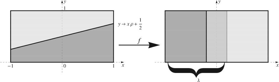
Figure 10.1. The map $f$ acting on the rectangle $[-1,1]\times[0,1]$.

Let $\nu_{\lambda,\rho}$ be the place-dependent invariant measure of the IFS on $[-1,1]$

$$\Psi_{\lambda}=\left\{\psi_{0}^{\lambda}(x)=\lambda x-(1-\lambda),\psi_{1}^{\lambda}(x)=\lambda x+(1-\lambda)\right\}$$

with probabilities $\left\{p_{0}(x)=\frac{1}{2}+\rho x,p_{1}(x)=\frac{1}{2}-\rho x\right\}$. That is, $\nu_{\lambda,\rho}$ is the unique probability measure of the dual operator $L^{*}$, where

$$Lg(x)=\left(\frac{1}{2}+\rho x\right)g(\lambda x-(1-\lambda))+\left(\frac{1}{2}-\rho x\right)g(\lambda x+(1-\lambda)),$$

for any continuous test function $g\colon[0,1]\mapsto\mathbb{R}$. In fact, by [12, Theorem 1.1],

(10.1) $$\lim_{n\to\infty}L^{n}g(x)=\int gd\nu_{\lambda,\rho}\text{ uniformly on $[0,1]$.}$$

Applying (10.1) and the bounded convergence theorem, simple calculations show that

$$\frac{1}{n}\sum_{k=0}^{n-1}\overline{\mathcal{L}}_{2}\circ f^{-k}\rightarrow\nu_{\lambda,\rho}\times\mathcal{L}_{1}\text{ weakly},$$

where $\overline{\mathcal{L}}_{2}$ is the normalized Lebesgue measure on the rectangle. Hence, by the results of Schmeling and Troubetzkoy [38, Section 2, 3], the measure $\nu_{\lambda,\rho}\times\mathcal{L}_{1}$ is the unique SBR-measure of the map $f$. Therefore, the property $\nu_{\mathrm{SBR}}\ll\mathcal{L}_{2}$ is equivalent to $\nu_{\lambda,\rho}\ll\mathcal{L}_{1}$ and moreover $\dim_{\rm H}\nu_{SBR}=1+\dim_{\rm H}\nu_{\lambda,\rho}$.

Clearly, the IFS $\Psi_{\lambda}$ satisfies the conditions (A1)-(A4) for $\lambda$ in an arbitrary compact subinterval of $(0,1)$. Moreover, it is easy to see that $\nu_{\lambda,\rho}$ is a push-forward measure of a parameter-dependent Gibbs measure $\mu_{\lambda,\rho}$. More precisely, let $\Omega=\{-1,1\}^{\mathbb{N}}$ and

$$\Pi^{\lambda}(\omega)=\sum_{k=1}^{\infty}\omega_{k}\lambda^{k-1},$$

and let $\phi^{\lambda}(\omega)=\log\left(p_{\omega_{1}}(\Pi^{\lambda}(\sigma\omega))\right)$. It is easy to see that $\phi^{\lambda}$ satisfies (3.1) and (3.2) for every fixed $\rho\in[0,1/2)$. Moreover,

$$\chi_{\mu_{\lambda,\rho}}=-\log\lambda;$$

$$h_{\mu_{\lambda,\rho}}=-\int_{\mathbb{R}}\left(\frac{1}{2}+\rho x\right)\log\left(\frac{1}{2}+\rho x\right)+\left(\frac{1}{2}-\rho x\right)\log\left(\frac{1}{2}-\rho x\right)d\nu_{\lambda,\rho}(x).$$

Shmerkin and Solomyak [41, Theorem 2.6] showed that $\Psi_{\lambda}$ satisfies the transversality condition (T) on the interval $\lambda\in(0,0.6684755)$. Hence we can apply Theorem 3.3 and verify the claim [1, Theorem 4.1].

Theorem 10.1.

For every $0\leq\rho<0.5$ and Lebesgue almost every $\lambda\in(0.5,0.6684755)$,

$$\dim_{\rm H}\nu_{\lambda,\rho}=\min\Bigl{\{}1,\frac{h_{\mu_{\lambda,\rho}}}{-\log\lambda}\Bigr{\}}$$

Moreover, $\nu_{\lambda,\rho}$ is absolutely continuous for Lebesgue almost every

$$\lambda\in\left\{\lambda\in(0.5,0.6684755):h_{\mu_{\lambda,\rho}}>-\log\lambda\right\}.$$

In particular, the region contains the quadrilateral formed by the points $(0,0.5)$, $(0.45,0.55)$, $(0.45,0.668)$, $(0,0.668)$.

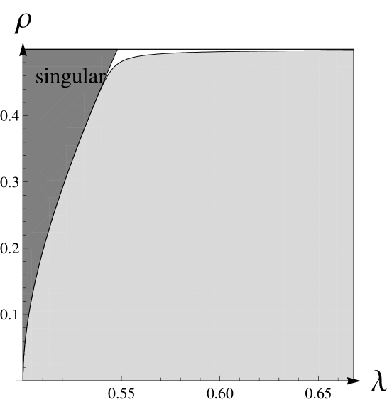
Figure 10.2. The singularity and absolute continuity region of the measure $\mu_{\lambda,\rho}$.

It follows from the calculations in [1], that for every $N\geq 1$,

(10.2) $$\log 2-\sum_{n=1}^{N}\frac{(2\rho)^{2n}}{2n(2n-1)}F_{n}-\frac{(2\rho)^{N+1}}{(2N+2)(2N+1)(1-(2\rho)^{2})}\leq h_{\mu_{\lambda,\rho}}\leq\log 2-\sum_{n=1}^{N}\frac{(2\rho)^{2n}}{2n(2n-1)}F_{n}.$$

where $F_{n}=\int x^{2n}d\mu_{\lambda,\rho}(x)$. The quantities $F_{n}$ can be expressed inductively by

$$F_{n}=\frac{(1-\lambda)^{2n}}{1+\lambda^{2n-1}(4n\rho(1-\lambda)-\lambda)}+\\ \sum_{m=1}^{n-1}\frac{2m(1-\lambda)^{2n-2m}\lambda^{2m-1}}{1+\lambda^{2n-1}(4n\rho(1-\lambda)-\lambda)}\binom{2n}{2m}\left(\frac{\lambda}{2m}-\frac{2\rho(1-\lambda)}{2n-2m+1}\right)F_{m}.$$

Using the estimates (10.2), we can approximate the region in Theorem 10.1, see Figure 10.2.

10.2. Blackwell measure for binary channel

Our second application is the absolute continuity of the Blackwell measure for a binary symmetric channel with a noise. Let us first introduce the basic notations, following Bárány, Pollicott and Simon [3] and Bárány and Kolossváry [2]. Let $X:=\left\{X_{i}\right\}_{i=-\infty}^{\infty}$ be a binary, symmetric, stationary, ergodic Markov chain source $X_{i}\in\left\{0,1\right\}$, with a probability transition matrix

$$\Pi:=\left[\begin{array}[]{cc}p&1-p\\ 1-p&p\\ \end{array}\right].$$

By adding to $X$ a binary independent and identically distributed (i.i.d.) noise $E=\left\{E_{i}\right\}_{i=-\infty}^{\infty}$ independent of $X$ with

$$\mathbb{P}(E_{i}=0)=1-\varepsilon,\qquad\mathbb{P}(E_{i}=1)=\varepsilon,$$

we get a Markov chain $Y:=\left\{Y_{i}\right\}_{i=-\infty}^{\infty}$, $Y_{i}=(X_{i},E_{i})$ with states $\{(0,0),(0,1),(1,0),\\ (1,1)\}$ and transition probabilities:

$$M:=\left[\begin{array}[]{cccc}p(1-\varepsilon)&p\varepsilon&(1-p)(1-\varepsilon)&(1-p)\varepsilon\\ p(1-\varepsilon)&p\varepsilon&(1-p)(1-\varepsilon)&(1-p)\varepsilon\\ (1-p)(1-\varepsilon)&(1-p)\varepsilon&p(1-\varepsilon)&p\varepsilon\\ (1-p)(1-\varepsilon)&(1-p)\varepsilon&p(1-\varepsilon)&p\varepsilon\\ \end{array}\right].$$

Let $\Psi:\left\{(0,0),(0,1),(1,0),(1,1)\right\}\mapsto\{0,1\}$ be a surjective map such that

$$\Psi(0,0)=\Psi(1,1)=0\text{ and }\Psi(0,1)=\Psi(1,0)=1.$$

We consider the ergodic stationary process $Z=\left\{Z_{i}=\Psi(Y_{i})\right\}_{i=-\infty}^{\infty}$, which is the corrupted output of the channel. Equivalently, $Z$ is the stationary stochastic process $Z_{i}=X_{i}\bigoplus E_{i}$, where $\bigoplus$ denotes the binary addition.

According to [14, Example 4.1] and [3, Example 1], the entropy of $Z$ can be expressed as follows. Consider the 3-dimensional simplex

$$W:=\Bigl{\{}\underline{w}\in\mathbb{R}^{4}:w_{i}\geq 0,\ \sum_{1\leq i\leq 4}w_{i}=1\Bigr{\}}$$

and define $W_{0},W_{1}\subset W$ by

$$W_{0}:=\left\{\underline{w}\in W:w_{2}=w_{3}=0\right\},\ W_{1}:=\left\{\underline{w}\in W:w_{1}=w_{4}=0\right\}.$$

Consider two matrices

$$M_{0}:=\left[\begin{array}[]{cccc}p(1-\varepsilon)&0&0&(1-p)\varepsilon\\ p(1-\varepsilon)&0&0&(1-p)\varepsilon\\ (1-p)(1-\varepsilon)&0&0&p\varepsilon\\ (1-p)(1-\varepsilon)&0&0&p\varepsilon\\ \end{array}\ \ \right]\text{ and }\ \ M_{1}:=\left[\begin{array}[]{cccc}0&p\varepsilon&(1-p)(1-\varepsilon)&0\\ 0&p\varepsilon&(1-p)(1-\varepsilon)&0\\ 0&(1-p)\varepsilon&p(1-\varepsilon)&0\\ 0&(1-p)\varepsilon&p(1-\varepsilon)&0\\ \end{array}\right],$$

and let $(r_{0}(\underline{w}),r_{1}(\underline{w}))$ be the place-dependent probability vector of the form

$$r_{i}(\underline{w})=\|\underline{w}^{T}M_{i}\|_{1},$$

where $\|.\|_{1}$ denotes the $l_{1}$ norm and $\underline{w}\in W$. Introduce two functions $f_{0}:W\mapsto W_{0}$ and $f_{1}:W\mapsto W_{1}$ such that

$$f_{i}(\underline{w})=\frac{\underline{w}^{T}M_{i}}{\|\underline{w}^{T}M_{i}\|_{1}}.$$

Then the entropy of $Z$ can be expressed as follows:

$$H(Z)=-\int_{W_{0}\cup W_{1}}\bigl{[}r_{0}(\underline{w})\log r_{0}(\underline{w})+r_{1}(\underline{w})\log r_{1}(\underline{w})\bigr{]}dQ(\underline{w}),$$

where the Blackwell measure $Q$ is the unique measure with $\mathrm{supp}(Q)\subseteq W_{0}\cup W_{1}$, such that for every continuous function $h\colon W_{0}\cup W_{1}\mapsto\mathbb{R}$,

$$\int h(\underline{w})dQ(\underline{w})=\int r_{0}(\underline{w})h(f_{0}(\underline{w}))+r_{1}(\underline{w})h(f_{1}(\underline{w}))dQ(\underline{w}).$$

It was shown in [3, Section 3.1, 3.2] that for the binary symmetric channel, the measure $Q$ on $W_{0}\cup W_{1}$ is conjugated to the place-dependent invariant probability measure $\nu_{\varepsilon,p}$ on $[0,1]$ for the IFS $\Psi_{\varepsilon,p}=\left\{S_{0}^{\varepsilon,p},S_{1}^{\varepsilon,p}\right\}$:

$$S_{0}^{\varepsilon,p}(x) :=\dfrac{x\cdot p\cdot(1-\varepsilon)+(1-x)\cdot(1-p)\cdot(1-\varepsilon)}{x\cdot\left[p(1-\varepsilon)+(1-p)\cdot\varepsilon\right]+(1-x)\cdot\left[(1-p)(1-\varepsilon)+p\cdot\varepsilon\right]},$$

$$S_{1}^{\varepsilon,p}(x) :=\dfrac{x\cdot p\cdot\varepsilon+(1-x)\cdot(1-p)\cdot\varepsilon}{x\cdot\left[p\varepsilon+(1-p)\cdot(1-\varepsilon)\right]+(1-x)\cdot\left[(1-p)\varepsilon+p\cdot(1-\varepsilon)\right]}.$$

and the place-dependent probability vector $(p_{0}^{\varepsilon,p}(x),p_{1}^{\varepsilon,p}(x))$:

$$p_{0}^{\varepsilon,p}(x) :=x\cdot\left[p(1-\varepsilon)+(1-p)\cdot\varepsilon\right]+(1-x)\cdot\left[(1-p)(1-\varepsilon)+p\cdot\varepsilon\right],$$

$$p_{1}^{\varepsilon,p}(x) :=x\cdot\left[p\varepsilon+(1-p)\cdot(1-\varepsilon)\right]+(1-x)\cdot\left[(1-p)\varepsilon+p\cdot(1-\varepsilon)\right].$$

In particular, $Q\ll\mathcal{L}_{1}|_{W_{0}\cup W_{1}}$ if and only if $\nu_{\varepsilon,p}\ll\mathcal{L}_{1}$.

Observe that for $\varepsilon=1/2$, $S_{0}^{\varepsilon,p}(x)=S_{1}^{\varepsilon,p}(x)=(2p-1)x+1-p$ and so $\nu_{\varepsilon,p}$ is the Dirac mass on the point $1/2$. Hence, we may assume that $\varepsilon\neq 1/2$.

For every fixed $\varepsilon\in(0,1)\setminus\{1/2\}$, the IFS $\Psi_{\varepsilon,p}$ satisfies the conditions (A1)-(A4) for $p$ in an arbitrary compact subinterval of $(0,1)$; and $\nu_{\varepsilon,p}$ is a push-forward measure of the Gibbs measure $\mu_{\varepsilon,p}$ with respect to the potential $\phi^{\varepsilon,p}(\omega)=\log\left(p_{\omega_{1}}^{\varepsilon,p}(\Pi^{\varepsilon,p}(\sigma\omega))\right)$ satisfying (3.1) and (3.2), where $\Pi^{\varepsilon,p}$ is the natural projection of the IFS $\Psi_{\varepsilon,p}$.

Bárány and Kolossváry [2] showed that for every fixed $\varepsilon\neq 1/2$ the IFS $\Psi_{\varepsilon,p}$ satisfies the transversality condition (T) with respect to the parameter $p$ and has $\frac{h_{\mu_{\varepsilon,p}}}{\chi_{\mu_{\varepsilon,p}}}>1$ on every interval $I$ for which $\{\varepsilon\}\times I$ is contained in the red region in Figure 10.3. Thus, the main theorem of the present paper applies and [2, Theorem 1.1] remains correct:

Theorem 10.2.

For every fixed $\varepsilon\in(0,1)\setminus\{1/2\}$ and for Lebesgue-almost every $p$ such that $(\varepsilon,p)\in R$ is in the red region of Figure 10.3, the measure $\nu^{\varepsilon,p}$ is absolutely continuous. For instance, the red region contains two quadrilaterals formed by $(0.5,0.75)$, $(0.37,0.775)$, $(0.5,0.795)$, $(0.63,0.775)$ and $(0.5,0.25),(0.37,0.225),(0.5,0.205),(0.63,0.225)$.

It was shown by Bárány, Pollicott and Simon [3] that $\mu_{\varepsilon,p}$ is singular in the blue region of Figure 10.3.

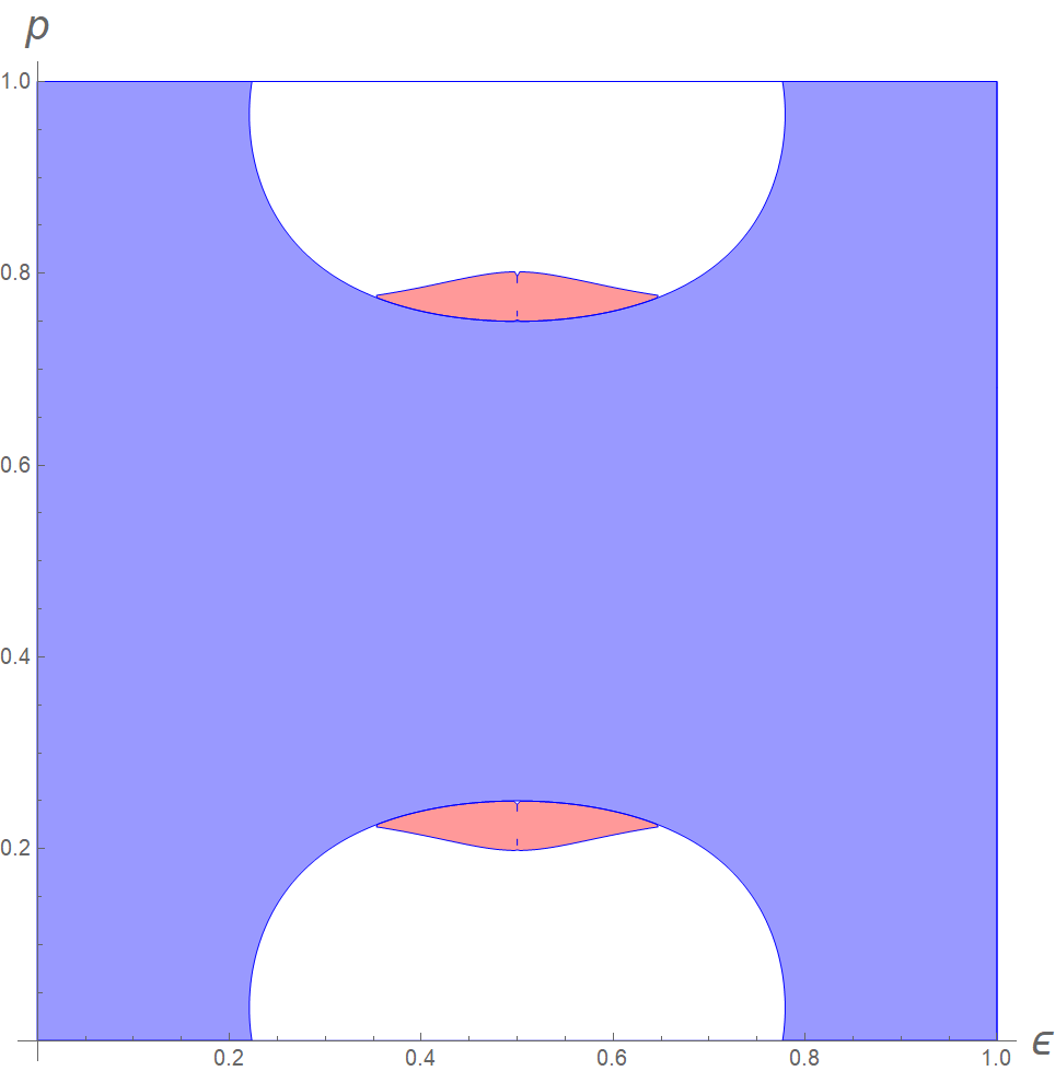
Figure 10.3. The singularity (blue) and transversality region with $\frac{h_{\mu_{\varepsilon,p}}}{\chi_{\mu_{\varepsilon,p}}}>1$ (red) of the measure $\nu_{\varepsilon,p}$, [2, Figure 1].

10.3. Absolute continuity of equilibrium measures for hyperbolic IFS with overlaps

First we recall briefly the notion of equilibrium measure in the setting of IFS. Let ${\mathcal{A}}=\{1,\ldots,m\}$ and suppose we have an IFS $\Psi=\{f_{j}\}_{j\in{\mathcal{A}}}$ of the class $C^{1+\theta}$ on a compact interval $X\subset\mathbb{R}$. We assume that that the system $\{f_{j}\}_{j\in{\mathcal{A}}}$ is uniformly hyperbolic and contractive:

(10.3) $$0<\gamma_{1}\leq|f_{j}^{\prime}(x)|\leq\gamma_{2}<1\ \ \mbox{for all}\ j\in{\mathcal{A}},\ x\in X.$$

As before, $\Omega={\mathcal{A}}^{\mathbb{N}}$ and $\sigma$ denotes the left shift on $\Omega$. We write $\Pi:\Omega\to\mathbb{R}$ for the natural projection map associated with the IFS. Consider the pressure function, defined by

(10.4) $$P_{\mathcal{A}}(t)=P_{\Psi}(t)=\lim_{n\to\infty}n^{-1}\log\sum_{u\in{\mathcal{A}}^{n}}\|f^{\prime}_{u}\|^{t}.$$

It is well-known that this limit exists, $t\mapsto P_{\mathcal{A}}(t)$ is continuous and strictly decreasing. According to the general theory of thermodynamical formalism (see e.g., [35]),

$$P_{\Psi}(t)=P(\sigma,t\phi),$$

where $\phi(\omega)=\log|f_{\omega_{1}}^{\prime}(\Pi(\sigma\omega))|$ is the potential associated with the IFS and $P(\sigma,\cdot)$ is the topological pressure. The equilibrium state for the potential $t\phi$ is a Borel probability measure $\mu$ on $\Omega$ satisfying

$$P_{\Psi}(t)=h_{\mu}+t\int\phi\,d\mu,$$

where $h_{\mu}=h_{\mu}(\sigma)$, see [35, 3.5]. Observe that $\int\phi\,d\mu=-\chi_{\mu}$ by the definition of the Lyapunov exponent. Denote by $s=s(\Psi)$ the solution of the Bowen’s equation:

(10.5) $$s=s(\Psi):\ \ P_{\Psi}(s)=0.$$

It is well-known that $s(\Psi)$ is the upper bound for the Hausdorff dimension of the attractor. We say that $\mu$ is an equilibrium measure for the IFS $\Psi$ if it is the equilibrium state for the potential $s(\Psi)\cdot\phi$. Thus, by definition,

$$\mu\ \mbox{is an equilibrium measure}\ \implies\ s(\Psi)=\frac{h_{\mu}}{\chi_{\mu}}\,.$$

The equilibrium measure is the dimension-maximizing measure for the IFS in the symbolic space. Under our assumptions, the equilibrium measure $\mu$ is the unique Gibbs measure for the potential $s\phi=s(\Psi)\cdot\phi$, which implies that

$$\mu([u])\asymp{\rm diam}([u])^{s},$$

for any cylinder set $[u]$ in $\Omega$. Here ${\rm diam}([u])$ is the diameter in the metric associated with the IFS: $d(\omega,\tau)=|X_{\omega\wedge\tau}|$. It follows that $\mu$ has local dimension $s$ at every point in $\Omega$; in particular, the correlation dimension $\dim_{\rm cor}(\mu)=s$.

Given a family of hyperbolic IFS $\Psi^{\lambda}$ (with overlaps) depending on a parameter $\lambda\in\overline{U}$, with equilibrium measure $\mu_{\lambda}$, we expect that typically, in the sense of almost every parameter, the projection of the equilibrium measure $(\Pi^{\lambda})_{*}\mu_{\lambda}$ has Hausdorff dimension $\min\{1,s(\Psi^{\lambda})\}$, and is absolutely continuous when $s(\Psi^{\lambda})>1$. This is what we prove under the assumptions of regularity and transversality. It is a simple consequence of Theorem 3.3, but we state it as a theorem because of its importance.

Theorem 10.3.

Let $\Psi^{\lambda}=\{f_{j}^{\lambda}\}_{j\in{\mathcal{A}}}$ be a parametrized IFS satisfying smoothness assumptions (A1) - (A4) and the transversality condition (T) on $U$. Let $\mu_{\lambda}$ be the equilibrium measure for $\Psi^{\lambda}$ and $s(\Psi^{\lambda})$ the solution of the Bowen’s equation (10.5). Then $\dim_{H}((\Pi^{\lambda})_{*}\mu_{\lambda})=\min\{1,s(\Psi^{\lambda})\}$ for a.e. $\lambda\in U$ and $(\Pi^{\lambda})_{*}\mu_{\lambda}$ is absolutely continuous with a density in $L^{2}$ for Lebesgue almost every $\lambda$ in the set $\{\lambda\in U:s(\Psi^{\lambda})>1\}$.

Proof.

As noted above, the equilibrium measure $\mu_{\lambda}$ satisfies $\dim_{cor}(\mu_{\lambda})=s(\Psi^{\lambda})$. By Theorem 3.1 and Theorem 3.2, it is enough to show that the equillibrium measure $\mu_{\lambda}$ satisfies (M). By Proposition 8.3, it is enough to show that potential $\phi^{\lambda}(\omega)=s(\Psi^{\lambda})\log\left|(f_{\omega_{1}}^{\lambda})^{\prime}(\Pi^{\lambda}(\sigma\omega))\right|$ satisfies (3.1) and (3.2).

The condition (3.1) is straightforward, since by assumption $\gamma_{1}<\left|(f_{\omega_{1}}^{\lambda})^{\prime}(\Pi^{\lambda}(\sigma\omega))\right|<\gamma_{2}$ on $U$ and trivially $s(\Psi^{\lambda})\leq\frac{\log m}{-\log\gamma_{2}}.$ On the other hand,

$$\begin{split}|\phi^{\lambda}(\omega)-\phi^{\tau}(\omega)|&=\Big{|}s(\Psi^{\lambda})\log\left|(f_{\omega_{1}}^{\lambda})^{\prime}(\Pi^{\lambda}(\sigma\omega))\right|\log\left|(f_{\omega_{1}}^{\lambda})^{\prime}(\Pi^{\lambda}(\sigma\omega))\right|-s(\Psi^{\tau})\log\left|(f_{\omega_{1}}^{\tau})^{\prime}(\Pi^{\tau}(\sigma\omega))\right|\Big{|}\\ &\leq-\log\gamma_{1}|s(\Psi^{\lambda})-s(\Psi^{\tau})|+\frac{\log m}{-\log\gamma_{2}}\Big{|}\log|(f_{\omega_{1}}^{\lambda})^{\prime}(\Pi^{\lambda}(\sigma\omega))|-\log\left|(f_{\omega_{1}}^{\tau})^{\prime}(\Pi^{\tau}(\sigma\omega))\right|\Big{|}\\ &\leq-\log\gamma_{1}|s(\Psi^{\lambda})-s(\Psi^{\tau})|+\frac{\log m}{-\gamma_{1}\log\gamma_{2}}\Big{|}(f_{\omega_{1}}^{\lambda})^{\prime}(\Pi^{\lambda}(\sigma\omega))-(f_{\omega_{1}}^{\tau})^{\prime}(\Pi^{\tau}(\sigma\omega))\Big{|}.\end{split}$$

By the assumptions (A1) - (A4), simple manipulation shows that $\lambda\mapsto(f_{\omega_{1}}^{\lambda})^{\prime}(\Pi^{\lambda}(\sigma\omega))$ is a Lipschitz map with Lipschitz constant independent of $\omega$. Hence, it is enough to show that $\lambda\mapsto s(\Psi^{\lambda})$ is Lipschitz. But clearly,

$$-\log\gamma_{2}|s-t|\leq|P_{\Phi^{\lambda}}(t)-P_{\Phi^{\lambda}}(s)|\leq-\log\gamma_{1}|s-t|,$$

and so

$$\begin{split}|s(\Psi^{\lambda})-s(\Psi^{\tau})|&\leq(-\log\gamma_{2})^{-1}|P_{\Phi^{\lambda}}(s(\Psi^{\lambda}))-P_{\Phi^{\lambda}}(s(\Psi^{\tau}))|\\ &=(-\log\gamma_{2})^{-1}|P_{\Phi^{\lambda}}(s(\Psi^{\tau}))-P_{\Phi^{\tau}}(s(\Psi^{\tau}))|\\ &\leq(-\log\gamma_{2})^{-1}c|\lambda-\tau|,\end{split}$$

where the last inequality follows by Lemma 8.2 since $\lambda\mapsto s(\Psi^{\tau})\log\left|(f_{\omega_{1}}^{\lambda})^{\prime}(\Pi^{\lambda}(\sigma\omega))\right|$ satisfies (3.2). ∎

10.4. Natural measures for non-homogeneous self-similar IFS

Consider a self-similar IFS on the line ${\mathcal{F}}=\{f_{j}(x)=r_{j}x+a_{j}\}_{j\in{\mathcal{A}}}$, where $r_{j}\in(0,1)$ and $a_{j}\in\mathbb{R}$. Recall that the similarity dimension is the number $s=s({\mathcal{F}})$, such that $\sum_{j\in{\mathcal{A}}}r_{j}^{s}=1$. Assume that the IFS is non-degenerate, in the sense that the fixed points of $f_{j}$ are all distinct. In this case the equilibrium measure is the Bernoulli product measure $({\mathbf{p}}^{\mathbb{N}})$ on $\Omega$, where ${\mathbf{p}}=(r_{1}^{s},\ldots,r_{m}^{s})$ is the vector of probability weights associated with the similarity dimension. We focus on the question of absolute continuity for the natural self-similar measure $\nu_{\mathcal{F}}=\Pi_{*}({\mathbf{p}}^{\mathbb{N}})$. (For the Hausdorff dimension $\dim_{H}(\nu_{\mathcal{F}})$ Hochman [15] obtained results that are much sharper than what we get with our method, so we don’t discuss the latter.) For non-homogeneous self-similar measures results on absolute continuity for a typical parameter in a “transversality region” were obtained by Neunhäuserer [26] and Ngai and Wang [27] independently. However, in their results the probabilities in the definition of self-similar measure are fixed, and so nothing can be claimed for the natural measure for a.e. parameter. More recently, Saglietti, Shmerkin, and Solomyak [37] proved absolute continuity for a.e. parameter in the entire “super-critical region” (i.e., where $h_{\mu}/\chi_{\mu}>1$), however, there also, probabilities are fixed, and an application of Fubini’s Theorem doesn’t yield anything for the natural measure. The following is an immediate consequence of Theorem 10.3.

Corollary 10.4.

Let ${\mathcal{F}}_{\lambda}=\{r_{j}(\lambda)x+a_{j}(\lambda)\}_{j\in{\mathcal{A}}}$ be a family of non-degenerate self-similar IFS satisfying smoothness assumptions (A1) - (A4) and the transversality condition (T) on $U$. Then the natural self-similar measure $\nu_{\lambda}$ is absolutely continuous with a density in $L^{2}$ for a.e. $\lambda\in U$ such that the similarity dimension is strictly greater than 1.

Specific regions where the transversality condition holds were found in [26, 27]. In particular, we have the following for the family of the IFS $\{\lambda_{1}x,\lambda_{2}+x\}$, where the 1-parameter family is obtained by assuming $\lambda=\lambda_{1},\ \lambda_{2}=c\lambda$ for a fixed $c>0$.

Corollary 10.5.

Let $\nu_{\lambda_{1},\lambda_{2}}$ be the natural self-similar measure for the IFS $\{\lambda_{1}x,\lambda_{2}x+1\}$. Then $\nu_{\lambda_{1},\lambda_{2}}$ is absolutely continuous with a density in $L^{2}$ for a.e. $(\lambda_{1},\lambda_{2})$ such that $\lambda_{1}+\lambda_{2}>1$ and $\max\{\lambda_{1},\lambda_{2}\}\leq 0.668$.

10.5. Some random continued fractions

Consider the IFS ${\mathcal{F}}_{\alpha,\beta}=\{f_{1},f_{2}\}=:\{\frac{x+\alpha}{x+\alpha+1},\frac{x+\beta}{x+\beta+1}\}$ on the real line, for $0\leq\alpha<\beta$. Applying the maps randomly (not necessarily independently), we obtain a random continued fraction $[1,Y_{1},1,Y_{2},1,Y_{3},\ldots]$ where $Y_{i}\in\{\alpha,\beta\}$ and we are using the notation

$$[a_{1},a_{2},a_{3},\ldots]:=\frac{1}{a_{1}+\displaystyle{\frac{1}{a_{2}+\displaystyle{\frac{1}{a_{3}+\ldots}}}}}$$

In the case $\alpha=0$ the IFS is parabolic; it was first studied by Lyons [23], motivated by a problem from the theory of Galton-Watson trees. In [44] it was shown that the invariant measure for the IFS corresponding to $Y_{i}$ applied i.i.d., with probabilities $(\frac{1}{2},\frac{1}{2})$ is absolutely continuous for a.e. $\beta\in(0.215,\beta_{c})$, where $\beta_{c}\in(0.2688,0.2689)$ is the “critical value”, such that

$$\frac{\log 2}{\chi_{\beta_{c}}}=1,$$

where $\chi_{\beta_{c}}$ is the Lyapunov exponent of the measure $(\frac{1}{2},\frac{1}{2})^{\mathbb{N}}$. Note that the IFS ${\mathcal{F}}_{0,\beta}$ is overlapping, i.e., its two cylinder intervals have non-trivial intersection, for $\beta\in(0,0.5)$.

In this paper we restrict ourselves to smooth hyperbolic IFS, so we need to take $\alpha>0$. However, we can take a very small positive $\alpha$ and expect somewhat similar behavior. The convex hull of the attractor for ${\mathcal{F}}_{\alpha,\beta}$ is the closed interval having the attracting fixed points of $f_{1},f_{2}$ as its endpoints; it is $X_{\alpha,\beta}=\Bigl{[}\frac{\sqrt{\alpha^{2}+4\alpha}-\alpha}{2},\frac{\sqrt{\beta^{2}+4\beta}-\beta}{2}\Bigr{]}.$ It is easy to check that the condition for the IFS to be overlapping, i.e., ${\mathcal{L}}^{1}\bigl{(}f_{1}(X_{\alpha,\beta})\cap f_{2}(X_{\alpha,\beta})\bigr{)}>0$ is

$$\beta+\alpha+4>3\bigl{(}\sqrt{\beta^{2}+4\beta}+\sqrt{\alpha^{2}+4\alpha}\bigr{)}.$$

It is satisfied, e.g., when $\alpha\in(0,10^{-4}]$ and $\beta\in(\alpha,0.485)$.

Example 10.6.

Denote by $\Pi^{\alpha,\beta}$ the natural projection from $\Omega=\{1,2\}^{\mathbb{N}}$ to the attractor and consider the equilibrium Gibbs measure $\mu_{\alpha,\beta}$ for the IFS. Fix $\alpha\in(0,10^{-4}]$ and $\beta=\sqrt{2}-1=0.41421\ldots$ Denote $\eta_{\alpha,\beta}:=\Pi^{\alpha,\beta}_{*}\mu_{\alpha,\beta}$. Then $\eta_{\alpha,\beta+\lambda}$ is absolutely continuous with a density in $L^{2}$ for a.e. $\lambda\in U=(0,0.485-\beta)\approx(0,0.077)$. ∎

In order to derive this claim from Theorem 10.3 we need to check transversality and that $h_{\mu_{\alpha,\beta}}/\chi_{\mu_{\alpha,\beta}}>1$ holds. (The regularity assumptions are obviously satisfied.) It is well-known that as soon as there is an overlap, the condition $s(\Psi_{\alpha,\beta})=h_{\mu_{\alpha,\beta}}/\chi_{\mu_{\alpha,\beta}}>1$ is satisfied, but for the reader’s convenience we provide a short proof in Appendix D, see Corollary D.3. Checking transversality is non-trivial; we indicate it in the next subsection. (In fact, we could get a larger interval of transversality $(\approx 0.215,0.485)$ for $\alpha\in(0,10^{-4}]$ with the method of [44, Section 6], which is more delicate.)

10.6. Checking transversality

Sometimes slightly different forms of the transversality conditions are used. Here they are:

(10.6) $$\begin{split}\exists&\,\eta>0:\ \forall\,u,v\in\Omega,\ \ u_{1}\neq v_{1},\ \lambda\in\overline{U}\\ &\qquad\left|\Pi^{\lambda}(u)-\Pi^{\lambda}(v)\right|\leq\eta\implies\left|\textstyle{\frac{d}{d\lambda}}(\Pi^{\lambda}(u)-\Pi^{\lambda}(v))\right|\geq\eta;\end{split}$$

(10.7) $$\begin{split}\exists&\,\eta>0:\ \forall\,u,v\in\Omega,\ \ u_{1}\neq v_{1},\ \lambda\in\overline{U}\\ &\qquad\Pi^{\lambda}(u)=\Pi^{\lambda}(v)\implies\left|\textstyle{\frac{d}{d\lambda}}(\Pi^{\lambda}(u)-\Pi^{\lambda}(v))\right|\geq\eta;\end{split}$$

(10.8) $$\begin{split}\exists&\,C_{T}>0:\ \forall\,u,v\in\Omega,\ \ u_{1}\neq v_{1},\ r>0\\ &\qquad{\mathcal{L}}^{1}\left\{\lambda\in\overline{U}:\ |\Pi^{\lambda}(u)-\Pi^{\lambda}(v)|\leq r\right\}\leq C_{T}\cdot r.\end{split}$$

Lemma 10.7.

Under regularity assumptions (A1) - (A4), all three conditions (10.6) - (10.8) are equivalent.

Proof.

The implication (10.6)$\implies$(10.7) is trivial.

The implication (10.6) $\implies$(10.8) is the usual transversality argument, see [43, Lemma 7.3].

Let us prove (10.8)$\implies$(10.7). We argue by contradiction. If (10.7) does not hold, we can use compactness of $\Omega$ and $\overline{U}$ and find $u,v\in\Omega$ with $u_{1}\neq v_{1}$, and $\lambda_{0}\in\overline{U}$ such that $F(\lambda)=\Pi^{\lambda}(u)-\Pi^{\lambda}(v)$ satisfies

$$F(\lambda_{0})=\frac{d}{d\lambda}F(\lambda_{0})=0.$$

Using that $\Pi^{\lambda}\in C^{1,\delta}$ (Proposition 4.3), we can write

$$|F(\lambda_{0}+t)| = |F(\lambda_{0}+t)-F(\lambda_{0})-F^{\prime}(\lambda_{0})t|$$

$$= |F^{\prime}(\lambda_{0}+\tau)t-F^{\prime}(\lambda_{0})t|\ \ \ \ \mbox{for some $\tau\in(0,t)$ by the Lagrange Theorem}$$

$$= |t|\cdot|F^{\prime}(\lambda_{0}+\tau)-F^{\prime}(\lambda_{0})|\leq|t|\cdot C_{\delta}|\tau|^{\delta}<C_{\delta}|t|^{1+\delta},$$

which clearly contradicts (10.8) for $r$ sufficiently small.

It remains to show (10.7)$\implies$(10.6), but this again follows by compactness of $\Omega$ and $\overline{U}$ and continuity of $\lambda\mapsto\Pi^{\lambda}$ and $\lambda\mapsto\frac{d}{d\lambda}\Pi^{\lambda}$. ∎

Next we consider two 1-parameter families of IFS for which it is possible to verify the transversality condition, under appropriate assumptions. They are variants and modifications of the parametrized families of IFS from [43, 44].

Proof of transversality in Example 10.6.

Let $f(x)=\frac{x}{x+1}$, so that ${\mathcal{F}}^{\lambda}=\{f(x+\alpha),f(x+\beta+\lambda)\}$, and let $\Pi^{\lambda}$ be the corresponding natural projection map. We can consider this IFS on $X=[0,0.5]$ for all these parameters. Here it is more convenient to verify the transversality condition in the form (10.7). Let $u,v\in\Omega$ with $u_{1}\neq v_{1}$. Without loss of generality we can assume that $u_{1}=2$ and $v_{1}=1$. Then we have by the Lagrange Theorem,

$$\Pi^{\lambda}(u)-\Pi^{\lambda}(v) = f\bigl{(}\beta+\lambda+\Pi^{\lambda}(\sigma u)\bigr{)}-f\bigl{(}\alpha+\Pi^{\lambda}(\sigma v)\bigr{)}$$

$$= f^{\prime}(c)\cdot\left[\beta-\alpha+\lambda+\Pi^{\lambda}(\sigma u)-\Pi^{\lambda}(\sigma v)\right]$$

$$=: f^{\prime}(c)\cdot\Psi^{\lambda}(u,v).$$

Since $f^{\prime}(c)\geq\gamma_{1}>0$, we obtain that

$$\left\{\lambda\in\overline{U}:\ |\Pi^{\lambda}(u)-\Pi^{\lambda}(v)|\leq r\right\}\subset\left\{\lambda\in\overline{U}:\ |\Psi^{\lambda}(u,v)|\leq r/\gamma_{1}\right\}.$$

In order to verify (10.8), it suffices to show that $\frac{d}{d\lambda}\Psi^{\lambda}(u,v)\geq\delta>0$. We have

(10.9) $$\textstyle{\frac{d}{d\lambda}}\Psi^{\lambda}(u,v)=1+\frac{d}{d\lambda}\Pi^{\lambda}(\sigma u)-\frac{d}{d\lambda}\Pi^{\lambda}(\sigma v)\geq 1-\frac{d}{d\lambda}\Pi^{\lambda}(\sigma v),$$

using monotonicity. We can write

$$\Pi^{\lambda}(\sigma v)=f_{1}^{i_{0}}f_{2}^{\lambda}f_{1}^{i_{1}}f_{2}^{\lambda}f_{1}^{i_{2}}f_{2}^{\lambda}\ldots$$

for some $i_{n}\geq 0$, where we write $f_{1}\equiv f_{1}^{\lambda}=f(x+\alpha)$ and $f_{2}^{\lambda}=f(x+\beta+\lambda)$, so that

$$\Pi^{\lambda}(\sigma v)=f_{1}^{i_{0}}f\bigl{(}\beta+\lambda+f_{1}^{i_{1}}f(\beta+\lambda+f_{1}^{i_{2}}\ldots)\bigr{)}.$$

Then simply using that $\|f_{1}^{\prime}\|_{\infty}<1$ and the maximum of the derivative is attained at the left endpoint by concavity, yields

$${\textstyle{\frac{d}{d\lambda}}}\Pi^{\lambda}(\sigma v)<f^{\prime}(\beta+\lambda)\Bigl{(}1+f^{\prime}(\beta+\lambda)\bigl{(}1+f^{\prime}(\beta+\lambda)(1+\cdots)\bigr{)}\Bigr{)}=\frac{f^{\prime}(\beta+\lambda)}{1-f^{\prime}(\beta+\lambda)}.$$

It remains to note that $f^{\prime}(\beta+\lambda)<f^{\prime}(\beta)=1/2$, hence ${\textstyle{\frac{d}{d\lambda}}}\Pi^{\lambda}(\sigma v)<1$, which implies the desired claim, in view of (10.9). ∎

10.7. “Vertical” translation family

Next we consider a class of 1-parameter families of IFS for which it is possible to verify the transversality condition, under appropriate assumptions. This is also a modification of the parametrized families of IFS from [43, 44].

Let $\{f_{j}\}_{j\in{\mathcal{A}}}$ be a $C^{1+\delta}$ IFS on $X$ and consider a “translation perturbation” $\{f_{j}^{\lambda}\}_{j\in{\mathcal{A}}}$, satisfying (A4), of the following form: assume that

$$\{f^{\lambda}_{j}(x)=f_{j}(x)+a_{j}(\lambda)\}_{j\in{\mathcal{A}}},$$

and assume that it is well-defined on $X$ for $\lambda\in\overline{U}$. We call it “vertical” because the graphs are translated vertically. Sometimes it is useful to consider IFS consisting of “horizontal” shifts of the same function, that is, IFS of the form $\{f(x+c_{j})\}_{j=1}^{m}$, like Example 10.6. Such families may be treated in a way similar to the “vertical” translation families with a few modifications, see [43, Section 7] and [44, Section 6]. Instead of treating this case in full generality, we focused on a specific example of random continued fractions above.

Denote for $i\neq j$ in ${\mathcal{A}}$:

(10.10) $$X_{ij}:=\left\{x\in X:\ \exists\,\lambda\in\overline{U},\ \exists\,y\in X\ \mbox{such that}\ f^{\lambda}_{i}(x)=f^{\lambda}_{j}(y)\right\}.$$

Note that $X_{ij}$ is empty if the corresponding 1st order cylinders never overlap. We further define, for $i\neq j$ in ${\mathcal{A}}$ such that $X_{ij}\neq\emptyset$:

(10.11) $${\|f^{\prime}_{i}\|}_{X_{ij}}:={\|f^{\prime}_{i}|_{X_{ij}}\|}_{\infty},\ \ \ \ \eta_{ij}:=\min\Bigl{|}\textstyle{\frac{d}{d\lambda}}\bigl{[}a_{i}(\lambda)-a_{j}(\lambda)\bigr{]}\Bigr{|}.$$

Let

(10.12) $$D_{\max}:=\max_{i}\Bigl{(}\frac{{\|\frac{d}{d\lambda}a_{i}\|}_{\infty}}{1-{\|f_{i}^{\prime}\|}_{\infty}}\Bigr{)}\,.$$

Proposition 10.8.

(i) If

(10.13) $$\eta_{ij}-\bigl{(}\|f^{\prime}_{i}\|_{X_{ij}}+\|f^{\prime}_{j}\|_{X_{ji}}\bigr{)}\cdot D_{\max}>0\ \ \ \mbox{for all $i\neq j$ such that $X_{ij}\neq\emptyset$},$$

then the transversality condition holds on $U$.

(ii) Assume, in addition, that $f_{j}^{\prime}(x)>0$ and $\frac{d}{d\lambda}a_{j}\geq 0$ for all $j\in{\mathcal{A}}$. If

(10.14) $$\eta_{ij}-\|f^{\prime}_{j}\|_{X_{ji}}\cdot D_{\max}>0\ \ \ \mbox{for all $i\neq j$ such that $X_{ij}\neq\emptyset$},$$

then the transversality condition holds on $U$.

Before the proof we present a more familiar special case. Let $\{f_{j}^{\lambda}\}_{j\in{\mathcal{A}}}$ be a $C^{1+\delta}$ IFS on $X$, satisfying (A4). Consider the translation family

$$\{f^{\lambda}_{1}(x)=f_{1}(x)+\lambda,\ f^{\lambda}_{j}(x)=f_{j}(x),\ j>1\},$$

and assume that it is well-defined on $X$ for $\lambda\in\overline{U}$. Note that only $f_{1}^{\lambda}$ changes with $\lambda$. Moreover, we assume that only the cylinder $f^{\lambda}_{1}(X)$ can intersect other 1-st order cylinders, that is

$$i\neq j,\ f_{i}(X)\cap f_{j}(X)\neq\emptyset\implies 1\in\{i,j\}.$$

Corollary 10.9.

(i) If

$$2{\|f^{\prime}_{1}\|}_{\infty}+{\|f^{\prime}_{j}\|}_{X_{j1}}<1\ \ \mbox{for all}\ \ 1<j\leq m,$$

then the transversality condition holds on $U$.

(ii) Assume, in addition, that $f_{j}^{\prime}(x)>0$ for all $j\in{\mathcal{A}}$. If

$${\|f^{\prime}_{1}\|}_{\infty}+{\|f^{\prime}_{j}\|}_{X_{j1}}<1\ \ \mbox{for all}\ \ 1<j\leq m,$$

then the transversality condition holds on $U$.

The derivation of the corollary from the proposition is immediate, since in this case we have $\eta_{1j}=1$ for $j>1$ and $D_{\max}=(1-{\|f^{\prime}_{1}\|}_{\infty})^{-1}$.

Proof of Proposition 10.8.

Consider the symbolic cylinder sets $[i]\subset\Omega$ and let

$$M_{\infty}:=\max_{u\in\Omega}\Bigl{\|}\textstyle{\frac{d}{d\lambda}}\Pi^{\lambda}(u)\Bigr{\|}_{\infty},\ \ \ M_{i}:=\max_{u\in[i]}\Bigl{\|}\frac{d}{d\lambda}\Pi^{\lambda}(u)\Bigr{\|}_{\infty},\ \ i\in{\mathcal{A}}.$$

We have

$$u\in[i]\implies\Pi^{\lambda}(u)=a_{i}(\lambda)+f_{i}(\Pi^{\lambda}(\sigma u)),$$

hence

(10.15) $$\frac{d}{d\lambda}\Pi^{\lambda}(u)=\frac{d}{d\lambda}a_{i}(\lambda)+f_{i}^{\prime}(\Pi^{\lambda}(\sigma u))\cdot\frac{d}{d\lambda}\Pi^{\lambda}(\sigma u)\ \ \ \mbox{for}\ \ u\in[i].$$

It follows that

$$M_{i}\leq\Bigl{\|}\textstyle{\frac{d}{d\lambda}}a_{i}(\lambda)\Bigr{\|}_{\infty}+{\|f^{\prime}_{i}\|}_{\infty}\cdot M_{\infty},$$

and since $M_{\infty}=\max_{i}M_{i}$, we obtain from (10.12) that

(10.16) $$M_{\infty}\leq D_{\max}.$$

Now we verify the transversality condition in the form (10.7). If $\Pi^{\lambda}(u)=\Pi^{\lambda}(v)$ and $u_{1}\neq v_{1}$, then $u\in[i]$ and $v\in[j]$ for some $i\neq j$ such that $X_{ij}\neq\emptyset$. Without loss of generality we can assume that $\frac{d}{d\lambda}\bigl{[}a_{i}(\lambda)-a_{j}(\lambda)\bigr{]}>0$ in the definition of $\eta_{ij}$, otherwise, exchange $i$ and $j$. Then (10.15) yields

(10.17) $$\frac{d}{d\lambda}\left(\Pi^{\lambda}(u)-\Pi^{\lambda}(v)\right)=\frac{d}{d\lambda}\bigl{[}a_{i}(\lambda)-a_{j}(\lambda)\bigr{]}+f_{i}^{\prime}(\Pi^{\lambda}(\sigma u))\cdot\frac{d}{d\lambda}\Pi^{\lambda}(\sigma u)-f_{j}^{\prime}(\Pi^{\lambda}(\sigma v))\cdot\frac{d}{d\lambda}\Pi^{\lambda}(\sigma v).$$

Note that

$$\Pi^{\lambda}(u)=f_{i}(\Pi^{\lambda}(\sigma u))=f_{j}(\Pi^{\lambda}(\sigma v))=\Pi^{\lambda}(v),$$

hence $\Pi^{\lambda}(\sigma u)\in X_{ij}$ and $\Pi^{\lambda}(\sigma v)\in X_{ji}$. Therefore, (10.17) yields

$$\left|\frac{d}{d\lambda}\left(\Pi^{\lambda}(u)-\Pi^{\lambda}(v)\right)\right|\geq\eta_{ij}-\bigl{(}\|f^{\prime}_{i}\|_{X_{ij}}+\|f^{\prime}_{j}\|_{X_{ji}}\bigr{)}\cdot D_{\max}>0,$$

assuming (10.13). This proves part (i) of the proposition.

In order to verify part (ii), note that if all $f_{j}$ and $\lambda\mapsto a_{j}(\lambda)$ are monotone increasing, we also get that $\frac{d}{d\lambda}\Pi^{\lambda}(u)\geq 0$ for all $u\in\Omega$, hence (10.17) implies

$$\left|\frac{d}{d\lambda}\left(\Pi^{\lambda}(u)-\Pi^{\lambda}(v)\right)\right|\geq\eta_{ij}-\|f^{\prime}_{j}\|_{X_{ji}}\cdot D_{\max}>0,$$

which is bounded away from zero under the assumption (10.13). This concludes the proof of (10.7) ∎

Example 10.10.

Let $\Psi:=\left\{f_{i}\right\}_{i=1}^{m}$ be a $C^{1+\delta}$ IFS on $X$. We assume that there exists a partition $\mathcal{A}=\mathcal{I}_{-1}\cup\mathcal{I}_{1}$ such that for very $i,j\in\mathcal{I}_{k}$, we have

(10.18) $$f_{i}(X)\cap f_{j}(X)=\emptyset,\quad i\neq j,\ i,j\in\mathcal{I}_{k},k=-1,1$$

Recall the definition of $\gamma_{2}$ from (A4). Besides (10.18), our second assumption is as follows:

(10.19) $$\gamma_{2}<\frac{1}{2}.$$

We define $\kappa(i)=k$ if $i\in\mathcal{I}_{k}$, $k=-1,1$. Then we introduce the family $\Psi^{\lambda}=\left\{f_{i}^{\lambda}\right\}_{i=1}^{m}$ with a parameter interval $\lambda\in U$, where

(10.20) $$f_{i}^{\lambda}(x):=f_{i}(x)+\kappa(i)\cdot\lambda.$$

Together with (10.19), this yields

(10.21) $$\left|\frac{d}{d\lambda}(a_{i}(\lambda)-a_{j}(\lambda))\right|\equiv\left\{\begin{array}[]{ll}2,&\hbox{if $\kappa(i)\neq\kappa(j)$;}\\ 0,&\hbox{if $\kappa(i)=\kappa(j)$.}\end{array}\right.\text{ and }D_{\max}\leq\frac{1}{1-\gamma_{2}}<2.$$

The parameter interval $U$ is an open interval centered at $0$, and $U$ is so small that

(10.22) $$f_{i}^{\lambda}(X)\subset\text{int}(X),\text{ and }f^{\lambda}_{i}(X)\cap f^{\lambda}_{j}(X)=\emptyset,\quad i\neq j,\ i,j\in\mathcal{I}_{k},\ k=-1,1,\ \lambda\in\overline{U}.$$

The (first level) cylinder intervals are $X_{i}^{\lambda}:=f_{i}^{\lambda}(X)$, $i\in\mathcal{A}$ and $\lambda\in U$. Observe that

(10.23) $$X_{ij}\neq\emptyset\Longleftrightarrow\exists\lambda\in\overline{U},\ X_{i}^{\lambda}\cap X_{j}^{\lambda}\neq\emptyset.$$

Using this and (10.21) we obtain

(10.24) $$X_{ij}\neq\emptyset\Longrightarrow\text{ either }\left(i\in\mathcal{I}_{-1}\ \&\ j\in\mathcal{I}_{1}\right)\text{ or }\left(j\in\mathcal{I}_{-1}\ \&\ i\in\mathcal{I}_{1}\right)\Longrightarrow\eta_{ij}=2.$$

Putting together this and the second part of (10.21) we obtain that (10.13) holds and consequently the transversality condition holds on $U$. ∎

Remark 10.11.

The partition $\mathcal{A}=\mathcal{I}_{-1}\cup\mathcal{I}_{1}$ satisfying (10.18) exists, for example, if every point in $X$ is covered by at most two level-1 cylinder intervals. That is

(10.25) $$\sum_{i=1}^{m}\mathds{1}_{f_{i}(X)}\leq 2.$$

In fact, let $[a_{j},b_{j}]:=X_{j}:=f_{j}(X)$. Without loss of generality, we may assume that the cylinder intervals $X_{j}$ are ordered in such a way that the left endpoints are in increasing order. If two level-1 cylinder intervals share the same left endpoint, that is, $a_{j}=a_{j+1}$, then we set $|X_{j}|\geq|X_{j+1}|$. Define $\mathcal{I}_{1}$ inductively, as follows: $1\in\mathcal{I}_{1}$. If the set $\mathcal{I}_{1}$ already contains $1=n_{1}<n_{2}<\cdots<n_{\ell}$, then we let $n_{\ell+1}:=\min\left\{j\in\mathcal{A}:\,b_{\ell}<a_{j}\right\}$, if such $a_{j}$ exists; otherwise, we stop and set $\mathcal{I}_{-1}:=\mathcal{A}\setminus\mathcal{I}_{1}$. It is easy to see that (10.18) holds.

Remark 10.12.

If we consider an IFS like in Example 10.10 but allow that every point is covered by at most $2\ell+1$ cylinder intervals for $\ell\geq 1$ and assume that $\gamma_{2}<\frac{1}{2\ell+1}$, then we get that the transversality condition holds in the same way. Namely, we can partition $\mathcal{A}$ into $2\ell+1$ families $\mathcal{I}_{-\ell},\dots\mathcal{I}_{\ell}$ in such a way that there are no intersections between distinct cylinder intervals from the same family. For all functions corresponding to the family $\mathcal{I}_{k}$ the translation is defined to be $k\cdot\lambda$. Then the minimal value of $\eta_{ij}$ is equal to 1 and $D_{\max}\leq\frac{\ell}{1-\gamma_{2}}$. This implies that (10.13) holds if $\gamma_{2}<\frac{1}{2\ell+1}$.

Definition 1.

We say that $\mathfrak{A}$ is a transversality-typical property of sufficiently smooth IFSs if the following holds: Whenever $\left\{\Psi^{\lambda}\right\}_{\lambda\in U}$ is a one-parameter family of sufficiently smooth IFSs for which the transversality condition holds then for $\mathcal{L}_{1}$ almost all $\lambda\in U$ the IFS $\Psi^{\lambda}$ has property $\mathfrak{A}$.

We use the notation of Example 10.10. In particular, we are given a compact interval $X\subset\mathbb{R}$ and a $C^{1+\delta}$ IFS $\left\{f_{i}\right\}_{i=1}^{m}$ on $X$ such that

(10.26) $$X_{i}:=f_{i}(X)\subset\mathrm{int}(X)\text{ for all }i\in\mathcal{A}.$$

Below we consider a translation perturbation family of $\Psi$. That is,

(10.27) $$\Psi^{\mathbf{t}}:=\left\{f_{i}^{\mathbf{t}}\right\}_{i=1}^{m},\quad f_{i}^{\mathbf{t}}(x):=f_{i}(x)+t_{i},\quad\mathbf{t}\in B(0,\delta_{0}),$$

where $\delta_{0}>0$ is so small that (10.26) holds if we replace $f_{i}$ with $f_{i}^{\mathbf{t}}$ and $X_{i}$ with $X_{i}^{\mathbf{t}}:=f_{i}^{\mathbf{t}}(X)$ for all $i\in\mathcal{A}$.

Claim.

Assume that

1. all points of $X$ are covered by at most two of the cylinder intervals $X_{k}$ and

2. $\gamma_{2}<1/2$.

Let $\mathfrak{A}$ be a transversality-typical property. Then there exists $0<\delta_{*}\leq\delta_{0}$ such that for $\mathcal{L}^{m}$-a.e. $\mathbf{t}\in B(0,\delta_{*})$, the translated IFS $\left\{\Psi^{\mathbf{t}}\right\}_{i=1}^{m}$ (defined in (10.27)) has property $\mathfrak{A}$.

Proof.

Using Remark 10.11, we can find a partition $\mathcal{A}=\mathcal{I}_{-1}\cup\mathcal{I}_{1}$ such that $f_{i}(X)\cap f_{j}(X)=\emptyset$ for distinct $i,j\in\mathcal{I}_{k}$, $k=-1,1$. Let $\delta_{1}>0$ be so small that $0<4\delta_{1}<\delta_{0}$ and

(10.28) $$X_{i}\cap X_{j}=\emptyset\Longrightarrow X^{t}_{i}\cap X^{t}_{j}=\emptyset\quad\text{ for all }\mathbf{t}\in B(0,4\delta_{1})$$

Hence

(10.29) $$X^{\mathbf{}}_{i}\cap X^{\mathbf{t}}_{j}=\emptyset,\quad i\neq j,\ i,j\in\mathcal{I}_{k},\ k=-1,1,\ \mathbf{t}\in B(0,4\delta_{1}).$$

Let $U:=(-\frac{1}{\sqrt{m}}\delta_{1},\frac{1}{\sqrt{m}}\delta_{1})$ and for a $\lambda\in U$ we define $\widetilde{\mathbf{a}}(\lambda):=(\kappa(1)\lambda,\dots,\kappa(m)\lambda)$, where we recall that $\kappa(i)=k$ if $i\in\mathcal{I}_{k}$. Finally, for a $\mathbf{t}\in B(0,\delta_{1})$ let

$$\mathbf{a}_{\mathbf{t}}(\lambda):=\mathbf{t}+\widetilde{\mathbf{a}}(\lambda).$$

Then $\|\mathbf{a}_{\mathbf{t}}(\lambda)\|<2\delta_{1},$ $\mathbf{t}\in B(0,\delta_{1}),\ \lambda\in U$. Hence

(10.30) $$X_{i}^{\mathbf{a}_{\mathbf{t}}(\lambda)}\subset X\quad\text{ and }\quad X_{i}^{\mathbf{a}_{\mathbf{t}}(\lambda)}\cap X_{j}^{\mathbf{a}_{\mathbf{t}}(\lambda)}=\emptyset,\ i\neq j,\ i,j\in\mathcal{I}_{k},\ k=-1,1,\ \lambda\in\overline{U}.$$

Example 10.10 shows that

(10.31) $$\text{ the transversality condition holds for the family }\left\{\Psi^{\mathbf{a}_{\mathbf{t}}(\lambda)}\right\}_{\lambda\in U}\quad\text{ for all }\mathbf{t}\in B(0,\delta_{1}).$$

Let

$$H:=\left\{\boldsymbol{\tau}\in B\left(0,\frac{\delta_{1}}{2\sqrt{m}}\right):\Psi^{\boldsymbol{\tau}}\text{ does not have property }\mathfrak{A}\right\}.$$

We need to prove that $\mathcal{L}^{m}(H)=0$. To get a contradiction assume that $\mathcal{L}^{m}(H)>0$. Then $H$ has a Lebesque density point $\widehat{\boldsymbol{\tau}}\in B(0,\frac{\delta_{1}}{2\sqrt{m}})$. Let $V$ be the intersection of $B\left(0,\frac{\delta_{1}}{2\sqrt{m}}\right)$ with the $(m-1)$-dimensional hyperplane which goes through the origin and is orthogonal to the vector $(\kappa(1),\dots,\kappa(m))$. Then by the Fubini theorem there exists a point $\mathbf{t}\in V$ such that $\mathcal{L}^{1}\left\{\lambda\in U:\mathbf{a}_{\mathbf{t}}(\lambda)\in H\right\}>0$. But this contradicts (10.31) and the fact that $\mathfrak{A}$ is a transversality-typical property. ∎

11. Open questions and further directions

As Theorem 3.2 guarantees more refined properties of $(\Pi^{\lambda})_{*}\mu_{\lambda}$ than mere absolute continuity, it is natural to ask whether a weaker condition than (M) is sufficient for an almost sure absolute continuity in the supercritical region $\left\{\lambda:\frac{h_{\mu_{\lambda}}}{\chi_{\mu_{\lambda}}}>1\right\}$. In particular, is (M0) sufficient? In our case, condition (M) is needed to guarantee regularity of the error term $e_{j}(\omega_{1},\omega_{2},\lambda)$ from (7.7), allowing us to follow the approach of Peres and Schlag [29].

Another natural direction of further research is to generalise the main result for multivariable parameters. Peres and Schlag in [29, Section 7] were handling this case for fixed (parameter independent) measures. In the case of parameter-dependent measures with one-dimensional family of parameters, we were using in the proof of Proposition 7.2 the Property (M) of the family of measures to provide proper estimates of the energy. The main issue in the case of multiparameter-dependent measures comes from the behaviour of the error term $e_{j}(\omega_{1},\omega_{2},\lambda)$. Namely, is it possible to follow [29, Lemma 7.10] and use the Property (M) to deduce similar estimates for the energy or higher regularity assumptions shall be made for the measures?

An application of the multiparameter case would be the natural equilibrium measure for self-conformal systems with translation parameters. Furthermore, one could study the absolute continuity of the Furstenberg measure induced by the Käenmäki measure (that is, the natural equilibrium measure for self-affine IFS, see [21]). For self-affine systems whose linear parts are strictly positive matrices the Käenmäki measure is a Gibbs measure which smoothly depends on the matrix elements, see Bárány and Rams [7] and Jurga and Morris [20]. The absolute continuity and the dimension of the Furstenberg measure induced by the Käenmäki measure plays a central role in the calculation of the dimension of the Käenmäki measure, see [7].

Another possible direction of further research is to study the absolute continuity of the SBR-measures of parametrized dynamical systems. Persson [32] considered a class of piecewise affine hyperbolic maps on a set $K\subset\mathbb{R}^{2}$, with one contracting and one expanding direction, which contains the class of the Belykh maps, as well as the fat baker’s transformations. The Belykh map, first introduced by Belykh [4] and later considered by Schmeling and Troubetzkoy [38] for a wider range of parameters, which contains the fat baker’s transformations as a special case.

For a parametrized family of Belykh maps, to prove the absolute continuity of an SBR-measure, one needs to show that the family of conditional measures over the stable foliation are absolutely continuous almost surely. Unlike the system defined in Subsection 10.1, the SBR-measure does not have a product structure, so the conditional measures of the stable directions depend not only on the parameters but also on the foliation itself. Persson [32] studied such systems, however, according to a personal communication [33], the proof contains a crucial error, similar to Bárány [1].

Extending our main results to the case of parabolic (and possibly infinite) iterated functions systems (as in [43, 44, 25]) is yet another possible research direction. It seems well motivated in the context of continued fractions expansion and would allow extending the results of Section 10.5 to their natural generality.

Appendix A Proof of Lemma 4.1

For $u=(u_{1},\ldots,u_{n})\in\Omega^{*}$ we have

(A.1) $$\frac{d}{dx}f^{\lambda}_{u}(x)=\prod\limits_{k=1}^{n}\left(\frac{d}{dx}f^{\lambda}_{u_{k}}\right)(f^{\lambda}_{\sigma^{k}u}x),$$

hence

(A.2) $$\frac{d^{2}}{dx^{2}}f^{\lambda}_{u}(x)=\left(\frac{d}{dx}f^{\lambda}_{u}(x)\right)\sum_{k=1}^{n}\frac{\left(\frac{d^{2}}{dx^{2}}f^{\lambda}_{u_{k}}\right)(f^{\lambda}_{\sigma^{k}u}(x))\cdot\frac{d}{dx}f^{\lambda}_{\sigma^{k}u}(x)}{\left(\frac{d}{dx}f^{\lambda}_{u_{k}}\right)(f^{\lambda}_{\sigma^{k}u}(x))}.$$

Applying (A1) and (A4) we obtain

(A.3) $$\left|\frac{\frac{d^{2}}{dx^{2}}f^{\lambda}_{u}(x)}{\frac{d}{dx}f^{\lambda}_{u}(x)}\right|\leq\frac{M_{1}}{\gamma_{1}}\sum\limits_{k=1}^{n}\left|\frac{d}{dx}f^{\lambda}_{\sigma^{k}u}(x)\right|\leq\frac{M_{1}}{\gamma_{1}}\sum\limits_{k=1}^{n}\gamma_{2}^{n-k}\leq\frac{M_{1}}{\gamma_{1}(1-\gamma_{2})}.$$

This proves (4.1). For the proof of (4.2), note first that differentiating (A.1) with respect to $\lambda$ gives

$$\frac{d^{2}}{d\lambda dx}f^{\lambda}_{u}(x)=\left(\frac{d}{dx}f^{\lambda}_{u}(x)\right)\sum_{k=1}^{n}\frac{\frac{d}{d\lambda}\left(\left(\frac{d}{dx}f^{\lambda}_{u_{k}}\right)(f^{\lambda}_{\sigma^{k}u}(x))\right)}{\left(\frac{d}{dx}f^{\lambda}_{u_{k}}\right)(f^{\lambda}_{\sigma^{k}u}(x))}.$$

Applying (A4) as before we get

(A.4) $$\left|\frac{\frac{d^{2}}{d\lambda dx}f^{\lambda}_{u}(x)}{\frac{d}{dx}f^{\lambda}_{u}(x)}\right|\leq\frac{1}{\gamma_{1}}\sum\limits_{k=1}^{n}\left|\frac{d}{d\lambda}\left(\left(\frac{d}{dx}f^{\lambda}_{u_{k}}\right)(f^{\lambda}_{\sigma^{k}u}(x))\right)\right|.$$

By (A1) and (A3) we have

(A.5) $$\left|\frac{d}{d\lambda}\left(\left(\frac{d}{dx}f^{\lambda}_{u_{k}}\right)(f^{\lambda}_{\sigma^{k}u}(x))\right)\right| \leq \left|\frac{d^{2}}{d\lambda dx}f^{\lambda}_{u_{k}}(f^{\lambda}_{\sigma^{k}u}(x))\right|+\left|\left(\frac{d^{2}}{dx^{2}}f^{\lambda}_{u_{k}}\right)(f^{\lambda}_{\sigma^{k}u}(x))\right|\cdot\left|\left(\frac{d}{d\lambda}f^{\lambda}_{\sigma^{k}u}\right)(x)\right|$$

$$\leq M_{2}+M_{1}|h_{k}(\lambda)|,$$

where $h_{k}(\lambda)=\frac{d}{d\lambda}f^{\lambda}_{\sigma^{k}u}(x)$. By (A2) we have $L=\sup\limits_{j\in{\mathcal{A}}}\sup\limits_{\lambda\in U}\left\|\frac{d}{d\lambda}f^{\lambda}_{j}\right\|_{\infty}<\infty$. Moreover, by (A4), we have for $1\leq k\leq n-1$

(A.6) $$|h_{k}(\lambda)| = \left|\frac{d}{d\lambda}\left(f^{\lambda}_{u_{k+1}}\left(f^{\lambda}_{\sigma^{k+1}u}(x)\right)\right)\right|$$

$$= \left|\left(\frac{d}{d\lambda}f^{\lambda}_{u_{k+1}}\right)\left(f^{\lambda}_{\sigma^{k+1}u}(x)\right)+\left(\frac{d}{dx}f^{\lambda}_{u_{k+1}}\right)\left(f^{\lambda}_{\sigma^{k+1}u}(x)\right)\cdot\left(\frac{d}{d\lambda}f^{\lambda}_{\sigma^{k+1}u}(x)\right)\right|$$

$$\leq L+\gamma_{2}|h_{k+1}(\lambda)|,$$

with $|h_{n}(\lambda)|=\left|\frac{d}{d\lambda}\mathrm{id}(x)\right|=0$. Therefore, iterating (A.6) yields

(A.7) $$|h_{k}(\lambda)|\leq L\sum\limits_{j=0}^{n-1-k}\gamma_{2}^{j}\leq\frac{L}{1-\gamma_{2}}.$$

Combining (A.4), (A.5), (A.6) and (A.7) gives

$$\left|\frac{\frac{d^{2}}{d\lambda dx}f^{\lambda}_{u}(x)}{\frac{d}{dx}f^{\lambda}_{u}(x)}\right|\leq\frac{(M_{2}+\frac{M_{1}L}{1-\gamma_{2}})n}{\gamma_{1}}.$$

This concludes the proof of Lemma 4.1.

Appendix B Some more regularity lemmas

Lemma B.1.

There exists a constant $C_{71}>0$ such that

$$\left|\frac{d}{d\lambda}f_{u}^{\lambda_{1}}(x)-\frac{d}{d\lambda}f_{u}^{\lambda_{2}}(x)\right|\leq C_{71}|\lambda_{1}-\lambda_{2}|^{\delta}$$

holds for all $\lambda_{1},\lambda_{2}\in U,\ x\in X,\ u\in\Omega^{*}$.

Proof.

We will prove the claim inductively with respect to $n=|u|$. More precisely, let us assume that

(B.1) $$\left|\frac{d}{d\lambda}f^{\lambda_{1}}_{u}(x)-\frac{d}{d\lambda}f^{\lambda_{2}}_{u}(x)\right|\leq C_{72}\sum\limits_{k=0}^{n-1}k\gamma_{2}^{k}|\lambda_{1}-\lambda_{2}|^{\delta}$$

holds for all $u\in{\mathcal{A}}^{n},\ \lambda_{1},\lambda_{2}\in U$ and $x\in X$ with some large enough constant $C_{72}$ (its value will be specified later). We shall prove that (B.1) holds also for $n+1$. Fix $u=(u_{1},\ldots,u_{n+1})\in{\mathcal{A}}^{n+1}$ and let $v=(u_{1},\ldots,u_{n})$. We have

$$\left|\frac{d}{d\lambda}f^{\lambda_{1}}_{u}(x)-\frac{d}{d\lambda}f^{\lambda_{2}}_{u}(x)\right| \leq \left|\left(\frac{d}{d\lambda}f^{\lambda_{1}}_{v}\right)\left(f^{\lambda_{1}}_{u_{n+1}}(x)\right)-\left(\frac{d}{d\lambda}f^{\lambda_{2}}_{v}\right)\left(f^{\lambda_{2}}_{u_{n+1}}(x)\right)\right|+$$

$$\bigg{|}\left(\left(\frac{d}{dx}f^{\lambda_{1}}_{v}\right)\left(f^{\lambda_{1}}_{u_{n+1}}(x)\right)\right)\left(\frac{d}{d\lambda}f^{\lambda_{1}}_{u_{n+1}}(x)\right)-$$

$$\left(\left(\frac{d}{dx}f^{\lambda_{2}}_{v}\right)\left(f^{\lambda_{2}}_{u_{n+1}}(x)\right)\right)\left(\frac{d}{d\lambda}f^{\lambda_{2}}_{u_{n+1}}(x)\right)\bigg{|}$$

$$=: A_{1}+A_{2}.$$

Let $L=\sup\limits_{j\in{\mathcal{A}}}\ \sup\limits_{\lambda\in U}\|\frac{d}{d\lambda}f^{\lambda}_{j}\|_{\infty}$. Assumption (A2) implies that $L$ is finite. By (B.1), (A2), (A3), (A4) and (4.2) we obtain

(B.2) $$A_{1} \leq \left|\left(\frac{d}{d\lambda}f^{\lambda_{1}}_{v}\right)\left(f^{\lambda_{1}}_{u_{n+1}}(x)\right)-\left(\frac{d}{d\lambda}f^{\lambda_{2}}_{v}\right)\left(f^{\lambda_{1}}_{u_{n+1}}(x)\right)\right|+$$

$$\left|\left(\frac{d}{d\lambda}f^{\lambda_{2}}_{v}\right)\left(f^{\lambda_{1}}_{u_{n+1}}(x)\right)-\left(\frac{d}{d\lambda}f^{\lambda_{2}}_{v}\right)\left(f^{\lambda_{2}}_{u_{n+1}}(x)\right)\right|$$

$$\leq C_{72}\sum\limits_{k=0}^{n-1}k\gamma_{2}^{k}|\lambda_{1}-\lambda_{2}|^{\delta}+\left\|\frac{d^{2}}{dxd\lambda}f^{\lambda_{2}}_{v}\right\|_{\infty}|f^{\lambda_{1}}_{u_{n+1}}(x)-f^{\lambda_{2}}_{u_{n+1}}(x)|$$

$$\leq C_{72}\sum\limits_{k=0}^{n-1}k\gamma_{2}^{k}|\lambda_{1}-\lambda_{2}|^{\delta}+LC_{52}n\left\|\frac{d}{dx}f^{\lambda_{2}}_{v}\right\|_{\infty}|\lambda_{1}-\lambda_{2}|$$

$$\leq C_{72}\sum\limits_{k=0}^{n-1}k\gamma_{2}^{k}|\lambda_{1}-\lambda_{2}|^{\delta}+LC_{52}n\gamma_{2}^{n}|\lambda_{1}-\lambda_{2}|.$$

Therefore, application of (A2) and (A4) gives

(B.3) $$A_{2} \leq \left|\left(\frac{d}{dx}f^{\lambda_{2}}_{v}\right)\left(f^{\lambda_{2}}_{u_{n+1}}(x)\right)\right|\cdot\left|\frac{d}{d\lambda}f^{\lambda_{1}}_{u_{n+1}}(x)-\frac{d}{d\lambda}f^{\lambda_{2}}_{u_{n+1}}(x)\right|+$$

$$\left|\frac{d}{d\lambda}f^{\lambda_{1}}_{u_{n+1}}(x)\right|\cdot\left|\left(\frac{d}{dx}f^{\lambda_{1}}_{v}\right)\left(f^{\lambda_{1}}_{u_{n+1}}(x)\right)-\left(\frac{d}{dx}f^{\lambda_{2}}_{v}\right)\left(f^{\lambda_{2}}_{u_{n+1}}(x)\right)\right|$$

$$\leq \gamma_{2}^{n}C_{3}|\lambda_{1}-\lambda_{2}|^{\delta}+L\left|\left(\frac{d}{dx}f^{\lambda_{1}}_{v}\right)\left(f^{\lambda_{1}}_{u_{n+1}}(x)\right)-\left(\frac{d}{dx}f^{\lambda_{2}}_{v}\right)\left(f^{\lambda_{2}}_{u_{n+1}}(x)\right)\right|$$

$$=: \gamma_{2}^{n}C_{3}|\lambda_{1}-\lambda_{2}|^{\delta}+LA_{3}$$

Furthermore, by Lemma 4.1, (A2) and (A4)

$$A_{3} \leq \left|\left(\frac{d}{dx}f^{\lambda_{1}}_{v}\right)\left(f^{\lambda_{1}}_{u_{n+1}}(x)\right)-\left(\frac{d}{dx}f^{\lambda_{1}}_{v}\right)\left(f^{\lambda_{2}}_{u_{n+1}}(x)\right)\right|+$$

$$\left|\left(\frac{d}{dx}f^{\lambda_{1}}_{v}\right)\left(f^{\lambda_{2}}_{u_{n+1}}(x)\right)-\left(\frac{d}{dx}f^{\lambda_{2}}_{v}\right)\left(f^{\lambda_{2}}_{u_{n+1}}(x)\right)\right|$$

$$\leq \left\|\frac{d^{2}}{dx^{2}}f^{\lambda_{1}}_{v}\right\|_{\infty}|f^{\lambda_{1}}_{u_{n+1}}(x)-f^{\lambda_{2}}_{u_{n+1}}(x)|+\sup\limits_{\lambda\in U}\left\|\left(\frac{d^{2}}{d\lambda dx}f^{\lambda}_{v}\right)\left(f^{\lambda_{2}}_{u_{n+1}}(x)\right)\right\|_{\infty}|\lambda_{1}-\lambda_{2}|$$

$$\leq C_{51}\left\|\frac{d}{dx}f^{\lambda_{1}}_{v}\right\|_{\infty}L|\lambda_{1}-\lambda_{2}|+C_{52}n\sup\limits_{\lambda\in U}\left\|\frac{d}{dx}f^{\lambda}_{v}\right\|_{\infty}|\lambda_{1}-\lambda_{2}|$$

$$\leq \left(LC_{51}+C_{52}n\right)\gamma_{2}^{n}|\lambda_{1}-\lambda_{2}|.$$

Combining the above inequality with (B.2) and (B.3) yields

$$\left|\frac{d}{d\lambda}f^{\lambda_{1}}_{u}(x)-\frac{d}{d\lambda}f^{\lambda_{1}}_{u}(x)\right|\leq C_{72}\sum\limits_{k=0}^{n}k\gamma_{2}^{k}|\lambda_{1}-\lambda_{2}|^{\delta},$$

provided $C_{72}$ is large enough. As (B.1) holds for $n=1$ by (A2), this concludes the inductive proof of (B.1) for $n\geq 1$. As $\sum\limits_{k=0}^{\infty}k\gamma_{2}^{k}<\infty$, the proof of the lemma is completed. ∎

Lemma B.2.

There exist constants $C_{75}>0,C_{76}>0$ such that

(B.4) $$\left|\frac{d^{2}}{dx^{2}}f_{u}^{\lambda_{1}}(x)-\frac{d^{2}}{dx^{2}}f_{u}^{\lambda_{2}}(x)\right|\leq C_{75}|u||\lambda_{1}-\lambda_{2}|^{\delta}\sup\limits_{\lambda\in[\lambda_{1},\lambda_{2}]}\left\|\frac{d}{dx}f^{\lambda}_{u}\right\|_{\infty}$$

and

(B.5) $$\left|\frac{d^{2}}{d\lambda dx}f_{u}^{\lambda_{1}}(x)-\frac{d^{2}}{d\lambda dx}f_{u}^{\lambda_{2}}(x)\right|\leq C_{76}|u|^{2}|\lambda_{1}-\lambda_{2}|^{\delta}\sup\limits_{\lambda\in[\lambda_{1},\lambda_{2}]}\left\|\frac{d}{dx}f^{\lambda}_{u}\right\|_{\infty}$$

hold for all $\lambda_{1},\lambda_{2}\in U,\ x\in X,\ u\in\Omega^{*}$.

Proof.

We shall prove (B.4). The proof of (B.5) is similar and we omit it. Let $n=|u|$. By (A.2) we have

(B.6) $$\bigg{|}\frac{d^{2}}{dx^{2}}f_{u}^{\lambda_{1}}(x) - \frac{d^{2}}{dx^{2}}f_{u}^{\lambda_{2}}(x)\bigg{|}\leq\left|\frac{d}{dx}f^{\lambda_{1}}_{u}(x)-\frac{d}{dx}f^{\lambda_{2}}_{u}(x)\right|\cdot\sum_{k=1}^{n}\left|\frac{\left(\frac{d^{2}}{dx^{2}}f^{\lambda_{1}}_{u_{k}}\right)(f^{\lambda_{1}}_{\sigma^{k}u}(x))\cdot\frac{d}{dx}f^{\lambda_{1}}_{\sigma^{k}u}(x)}{\left(\frac{d}{dx}f^{\lambda_{1}}_{u_{k}}\right)(f^{\lambda_{1}}_{\sigma^{k}u}(x))}\right|+$$

$$\left|\frac{d}{dx}f_{u}^{\lambda_{2}}(x)\right|\cdot\sum_{k=1}^{n}\left|\frac{\left(\frac{d^{2}}{dx^{2}}f^{\lambda_{1}}_{u_{k}}\right)(f^{\lambda_{1}}_{\sigma^{k}u}(x))\cdot\frac{d}{dx}f^{\lambda_{1}}_{\sigma^{k}u}(x)}{\left(\frac{d}{dx}f^{\lambda_{1}}_{u_{k}}\right)(f^{\lambda_{1}}_{\sigma^{k}u}(x))}-\frac{\left(\frac{d^{2}}{dx^{2}}f^{\lambda_{2}}_{u_{k}}\right)(f^{\lambda_{2}}_{\sigma^{k}u}(x))\cdot\frac{d}{dx}f^{\lambda_{2}}_{\sigma^{k}u}(x)}{\left(\frac{d}{dx}f^{\lambda_{2}}_{u_{k}}\right)(f^{\lambda_{2}}_{\sigma^{k}u}(x))}\right|$$

$$=: A_{1}\cdot A_{2}+\left|\frac{d}{dx}f_{u}^{\lambda_{2}}(x)\right|\cdot\sum\limits_{k=1}^{n}h_{k}(x).$$

We will bound now the above terms. First, by (4.2) and the mean value theorem, we have

$$A_{1}\leq\left|\frac{d^{2}}{d\lambda dx}f^{\xi}_{u}(x)\right|\left|\lambda_{1}-\lambda_{2}\right|\leq C_{52}|u|\left|\lambda_{1}-\lambda_{2}\right|\sup_{\lambda\in[\lambda_{1},\lambda_{2}]}\left|\frac{d}{dx}f^{\lambda}_{u}(x)\right|,$$

where $\xi\in U$ is a point lying between $\lambda_{1}$ and $\lambda_{2}$. By (A.3) (recall (A.2))

$$A_{2}\leq\frac{M_{1}}{\gamma_{1}(1-\gamma_{2})}.$$

Reducing the expression defining $h_{k}(x)$ to a common denominator and applying (A4) gives

$$h_{k}(x) \leq \frac{1}{\gamma_{1}^{2}}\bigg{|}\left(\frac{d}{dx}f^{\lambda_{2}}_{u_{k}}\right)(f^{\lambda_{2}}_{\sigma^{k}u}(x))\cdot\left(\frac{d^{2}}{dx^{2}}f^{\lambda_{1}}_{u_{k}}\right)(f^{\lambda_{1}}_{\sigma^{k}u}(x))\cdot\frac{d}{dx}f^{\lambda_{1}}_{\sigma^{k}u}(x)$$

$$- \left(\frac{d}{dx}f^{\lambda_{1}}_{u_{k}}\right)(f^{\lambda_{1}}_{\sigma^{k}u}(x))\cdot\left(\frac{d^{2}}{dx^{2}}f^{\lambda_{2}}_{u_{k}}\right)(f^{\lambda_{2}}_{\sigma^{k}u}(x))\cdot\frac{d}{dx}f^{\lambda_{2}}_{\sigma^{k}u}(x)\bigg{|}$$

$$\leq \frac{1}{\gamma_{1}^{2}}\Bigg{(}\bigg{|}\left(\frac{d}{dx}f^{\lambda_{2}}_{u_{k}}\right)(f^{\lambda_{2}}_{\sigma^{k}u}(x))-\left(\frac{d}{dx}f^{\lambda_{1}}_{u_{k}}\right)(f^{\lambda_{1}}_{\sigma^{k}u}(x))\bigg{|}\cdot\bigg{|}\left(\frac{d^{2}}{dx^{2}}f^{\lambda_{1}}_{u_{k}}\right)(f^{\lambda_{1}}_{\sigma^{k}u}(x))\cdot\frac{d}{dx}f^{\lambda_{1}}_{\sigma^{k}u}(x)\bigg{|}\ +$$

$$\bigg{|} \left(\frac{d}{dx}f^{\lambda_{1}}_{u_{k}}\right)(f^{\lambda_{1}}_{\sigma^{k}u}(x))\bigg{|}\cdot\bigg{|}\left(\frac{d^{2}}{dx^{2}}f^{\lambda_{1}}_{u_{k}}\right)(f^{\lambda_{1}}_{\sigma^{k}u}(x))\cdot\frac{d}{dx}f^{\lambda_{1}}_{\sigma^{k}u}(x)-\left(\frac{d^{2}}{dx^{2}}f^{\lambda_{2}}_{u_{k}}\right)(f^{\lambda_{2}}_{\sigma^{k}u}(x))\cdot\frac{d}{dx}f^{\lambda_{2}}_{\sigma^{k}u}(x)\bigg{|}\Bigg{)}$$

$$=: \frac{1}{\gamma^{2}}\left(A_{3}\cdot A_{4}+A_{5}\cdot A_{6}\right).$$

By (A1), (A3), (4.1) we have

$$A_{3} \leq \bigg{|}\left(\frac{d}{dx}f^{\lambda_{2}}_{u_{k}}\right)(f^{\lambda_{2}}_{\sigma^{k}u}(x))-\left(\frac{d}{dx}f^{\lambda_{1}}_{u_{k}}\right)(f^{\lambda_{2}}_{\sigma^{k}u}(x))\bigg{|}+\bigg{|}\left(\frac{d}{dx}f^{\lambda_{1}}_{u_{k}}\right)(f^{\lambda_{2}}_{\sigma^{k}u}(x))-\left(\frac{d}{dx}f^{\lambda_{1}}_{u_{k}}\right)(f^{\lambda_{1}}_{\sigma^{k}u}(x))\bigg{|}$$

$$\leq \left|\lambda_{1}-\lambda_{2}\right|\sup_{\lambda\in[\lambda_{1},\lambda_{2}]}\left|\left(\frac{d^{2}}{d\lambda dx}f^{\lambda}_{u_{k}}\right)(f^{\lambda_{2}}_{\sigma^{k}u}(x))\right|+\left\|\frac{d^{2}}{dx^{2}}f^{\lambda_{1}}_{u_{k}}\right\|_{\infty}|f^{\lambda_{2}}_{\sigma^{k}u}(x)-f^{\lambda_{1}}_{\sigma^{k}u}(x)|$$

$$\leq M_{2}|\lambda_{1}-\lambda_{2}|+M_{1}|\lambda_{1}-\lambda_{2}|\sup\limits_{\lambda\in[\lambda_{1},\lambda_{2}]}\left|\frac{d}{d\lambda}f^{\lambda}_{\sigma^{k}u}(x)\right|\leq M_{11}|\lambda_{1}-\lambda_{2}|,$$

for some constant $M_{11}>0$, as $\sup\limits_{\lambda\in U}\left|\frac{d}{d\lambda}f^{\lambda}_{\sigma^{k}u}(x)\right|$ is bounded uniformly in $u\in\Omega^{*},1\leq k\leq n$ and $x\in X$ by Lemma B.1. Assumptions (A1) and (A4) imply

$$A_{4}\leq M_{1}\gamma_{2}^{n-k}\text{ and }A_{5}\leq\gamma_{2}.$$

Applying (A1), (A4), (4.2), Lemma B.1 gives

$$A_{6} \leq \bigg{|}\left(\frac{d^{2}}{dx^{2}}f^{\lambda_{1}}_{u_{k}}\right)(f^{\lambda_{1}}_{\sigma^{k}u}(x))\bigg{|}\cdot\bigg{|}\frac{d}{dx}f^{\lambda_{1}}_{\sigma^{k}u}(x)-\frac{d}{dx}f^{\lambda_{2}}_{\sigma^{k}u}(x)\bigg{|}+$$

$$\bigg{|}\left(\frac{d^{2}}{dx^{2}}f^{\lambda_{1}}_{u_{k}}\right)(f^{\lambda_{1}}_{\sigma^{k}u}(x))-\left(\frac{d^{2}}{dx^{2}}f^{\lambda_{2}}_{u_{k}}\right)(f^{\lambda_{2}}_{\sigma^{k}u}(x))\bigg{|}\cdot\bigg{|}\frac{d}{dx}f^{\lambda_{2}}_{\sigma^{k}u}(x)\bigg{|}$$

$$\leq M_{1}|\lambda_{1}-\lambda_{2}|\sup\limits_{\lambda\in[\lambda_{1},\lambda_{2}]}\left|\frac{d^{2}}{dxd\lambda}f^{\lambda}_{\sigma^{k}u}(x)\right|+$$

$$\gamma_{2}^{n-k}\bigg{|}\left(\frac{d^{2}}{dx^{2}}f^{\lambda_{1}}_{u_{k}}\right)(f^{\lambda_{1}}_{\sigma^{k}u}(x))-\left(\frac{d^{2}}{dx^{2}}f^{\lambda_{2}}_{u_{k}}\right)(f^{\lambda_{2}}_{\sigma^{k}u}(x))\bigg{|}$$

$$\leq M_{1}|n-k|\gamma_{2}^{n-k}|\lambda_{1}-\lambda_{2}|+\gamma_{2}^{n-k}A_{7}$$

and again by (A1) and Lemma B.1

$$A_{7} \leq \bigg{|}\left(\frac{d^{2}}{dx^{2}}f^{\lambda_{1}}_{u_{k}}\right)(f^{\lambda_{1}}_{\sigma^{k}u}(x))-\left(\frac{d^{2}}{dx^{2}}f^{\lambda_{1}}_{u_{k}}\right)(f^{\lambda_{2}}_{\sigma^{k}u}(x))\bigg{|}+$$

$$\bigg{|}\left(\frac{d^{2}}{dx^{2}}f^{\lambda_{1}}_{u_{k}}\right)(f^{\lambda_{2}}_{\sigma^{k}u}(x))-\left(\frac{d^{2}}{dx^{2}}f^{\lambda_{2}}_{u_{k}}\right)(f^{\lambda_{2}}_{\sigma^{k}u}(x))\bigg{|}$$

$$\leq C_{1}|f^{\lambda_{1}}_{\sigma^{k}u}(x)-f^{\lambda_{2}}_{\sigma^{k}u}(x)|^{\delta}+C_{2}|\lambda_{1}-\lambda_{2}|^{\delta}$$

$$\leq C_{1}|\lambda_{1}-\lambda_{2}|^{\delta}\sup\limits_{\lambda\in[\lambda_{1},\lambda_{2}]}\left|\frac{d}{d\lambda}f^{\lambda}_{\sigma^{k}u}(x)\right|^{\delta}+C_{2}|\lambda_{1}-\lambda_{2}|^{\delta}\leq M_{12}|\lambda_{1}-\lambda_{2}|^{\delta}.$$

Combining the above with (B.6), bound on $h_{k}$ and estimates on $A_{1},\ldots,A_{7}$ and recalling that $\sum\limits_{k=1}^{n}|n-k|\gamma_{2}^{n-k}\leq\sum\limits_{k=0}^{\infty}k\gamma_{2}^{k}<\infty$ finishes the proof of (B.4). ∎

Appendix C Proof of Proposition 4.5

We will write $d(u,v)$ for $d_{\lambda_{0}}(u,v)$. Let $n=|u\wedge v|$, so that $u\wedge v=u_{1}\ldots u_{n}$. Let us begin by proving (4.8). We have

(C.1) $$\textstyle{\frac{d}{d\lambda}}(\Pi^{\lambda}(u)-\Pi^{\lambda}(v)) = \textstyle{\frac{d}{d\lambda}}\left[f_{u\wedge v}^{\lambda}(\Pi^{\lambda}(\sigma^{n}u))-f_{u\wedge v}^{\lambda}(\Pi^{\lambda}(\sigma^{n}v))\right]$$

$$= \left(\textstyle{\frac{d}{d\lambda}}f_{u\wedge v}^{\lambda}\right)(\Pi^{\lambda}(\sigma^{n}u))-\left(\textstyle{\frac{d}{d\lambda}}f_{u\wedge v}^{\lambda}\right)(\Pi^{\lambda}(\sigma^{n}v))+$$

$$\left(\textstyle{\frac{d}{dx}}f_{u\wedge v}^{\lambda}\right)(\Pi^{\lambda}(\sigma^{n}u))\cdot\textstyle{\frac{d}{d\lambda}}\Pi^{\lambda}(\sigma^{n}u)-\left(\textstyle{\frac{d}{dx}}f_{u\wedge v}^{\lambda}\right)(\Pi^{\lambda}(\sigma^{n}v))\cdot\textstyle{\frac{d}{d\lambda}}\Pi^{\lambda}(\sigma^{n}v)$$

$$= \left(\textstyle{\frac{d}{d\lambda}}f_{u\wedge v}^{\lambda}\right)(\Pi^{\lambda}(\sigma^{n}u))-\left(\textstyle{\frac{d}{d\lambda}}f_{u\wedge v}^{\lambda}\right)(\Pi^{\lambda}(\sigma^{n}v))+$$

$$\left(\textstyle{\frac{d}{dx}}f_{u\wedge v}^{\lambda}\right)(\Pi^{\lambda}(\sigma^{n}u))\cdot\left[\textstyle{\frac{d}{d\lambda}}\left(\Pi^{\lambda}(\sigma^{n}u)-\Pi^{\lambda}(\sigma^{n}v)\right)\right]+$$

$$\left[\left(\textstyle{\frac{d}{dx}}f_{u\wedge v}^{\lambda}\right)(\Pi^{\lambda}(\sigma^{n}u))-\left(\textstyle{\frac{d}{dx}}f_{u\wedge v}^{\lambda}\right)(\Pi^{\lambda}(\sigma^{n}v))\right]\cdot\textstyle{\frac{d}{d\lambda}}\Pi^{\lambda}(\sigma^{n}v)$$

$$=: A_{1}+A_{2}+A_{3}.$$

Application of (4.2), Lemma 4.4 and (A4) yields

$$|A_{1}| \leq \left\|\frac{d^{2}}{dxd\lambda}f^{\lambda}_{u\wedge v}\right\|_{\infty}|\Pi^{\lambda}(\sigma^{n}u)-\Pi^{\lambda}(\sigma^{n}v)|\leq C_{52}n\left\|\frac{d}{dx}f^{\lambda}_{u\wedge v}\right\|_{\infty}\leq\frac{C_{52}}{c_{1}}nd(u,v)^{1-\beta/4}$$

$$\leq \frac{C_{52}}{c_{1}}n\gamma_{2}^{3n\beta/4}d(u,v)^{1-\beta}\leq\frac{C_{\beta,1}}{3}d(u,v)^{1-\beta},$$

provided $C_{\beta,1}$ is chosen large enough. Using Lemma 4.4 together with the fact that $\frac{d}{d\lambda}\Pi^{\lambda}$ is bounded on $U\times\Omega$ (following from Proposition 4.3), one obtains

$$|A_{2}|\leq\frac{C_{\beta,1}}{3}d(u,v)^{1-\beta/4}\leq\frac{C_{\beta,1}}{3}d(u,v)^{1-\beta},$$

if $C_{\beta,1}$ is large enough. Boundedness of $\frac{d}{d\lambda}\Pi^{\lambda}$, (4.1) and Lemma 4.4 imply

$$|A_{3}| \leq \left\|\frac{d^{2}}{dx^{2}}f^{\lambda}_{u\wedge v}\right\|_{\infty}|\Pi^{\lambda}(\sigma^{n}u)-\Pi^{\lambda}(\sigma^{n}v)|\left|\textstyle{\frac{d}{d\lambda}}\Pi^{\lambda}(\sigma^{n}v)\right|\leq C_{51}\left\|\frac{d}{dx}f^{\lambda}_{u\wedge v}\right\|_{\infty}\left|\textstyle{\frac{d}{d\lambda}}\Pi^{\lambda}(\sigma^{n}v)\right|$$

$$\leq \frac{C_{\beta,1}}{3}d(u,v)^{1-\beta},$$

once again for $C_{\beta,1}$ large enough. This finishes the proof of (4.8). For the proof of (4.9), let us write a decomposition analogous to (C.1):

$$\frac{d}{d\lambda}\left(\Pi^{\lambda_{1}}(u)-\Pi^{\lambda_{1}}(v)\right)-\frac{d}{d\lambda}\left(\Pi^{\lambda_{2}}(u)-\Pi^{\lambda_{2}}(v)\right)=\left(A_{1}^{\lambda_{1}}-A_{1}^{\lambda_{2}}\right)+\left(A_{2}^{\lambda_{1}}-A_{2}^{\lambda_{2}}\right)+\left(A_{3}^{\lambda_{1}}-A_{3}^{\lambda_{2}}\right).$$

We have

(C.2) $$|A_{1}^{\lambda_{1}}-A_{1}^{\lambda_{2}}| = \left|\int\limits_{\Pi^{\lambda_{1}}(\sigma^{n}v)}^{\Pi^{\lambda_{1}}(\sigma^{n}u)}\frac{d^{2}}{dxd\lambda}f^{\lambda_{1}}_{u\wedge v}(y)dy-\int\limits_{\Pi^{\lambda_{2}}(\sigma^{n}v)}^{\Pi^{\lambda_{2}}(\sigma^{n}u)}\frac{d^{2}}{dxd\lambda}f^{\lambda_{2}}_{u\wedge v}(y)dy\right|$$

$$\leq \int\limits_{S}\left|\frac{d^{2}}{dxd\lambda}f^{\lambda_{1}}_{u\wedge v}(y)-\frac{d^{2}}{dxd\lambda}f^{\lambda_{2}}_{u\wedge v}(y)\right|dy+\int\limits_{S_{1}}\left|\frac{d^{2}}{dxd\lambda}f^{\lambda_{1}}_{u\wedge v}(y)\right|dy+\int\limits_{S_{2}}\left|\frac{d^{2}}{dxd\lambda}f^{\lambda_{2}}_{u\wedge v}(y)\right|dy,$$

where

$$S = [\Pi^{\lambda_{1}}(\sigma^{n}u),\Pi^{\lambda_{1}}(\sigma^{n}v)]\cap[\Pi^{\lambda_{2}}(\sigma^{n}u),\Pi^{\lambda_{2}}(\sigma^{n}v)],$$

$$S_{1} = [\Pi^{\lambda_{1}}(\sigma^{n}u),\Pi^{\lambda_{1}}(\sigma^{n}v)]\setminus[\Pi^{\lambda_{2}}(\sigma^{n}u),\Pi^{\lambda_{2}}(\sigma^{n}v)],$$

$$S_{2} = [\Pi^{\lambda_{2}}(\sigma^{n}u),\Pi^{\lambda_{2}}(\sigma^{n}v)]\setminus[\Pi^{\lambda_{2}}(\sigma^{n}u),\Pi^{\lambda_{2}}(\sigma^{n}v)].$$

Set $L=\sup\limits_{\lambda\in U}\sup\limits_{u\in\Omega}\left|\frac{d}{d\lambda}\Pi^{\lambda}(u)\right|$. We have then $|\Pi^{\lambda_{1}}(\sigma^{n}u)-\Pi^{\lambda_{2}}(\sigma^{n}u)|\leq L|\lambda_{1}-\lambda_{2}|$ and $|\Pi^{\lambda_{1}}(\sigma^{n}v)-\Pi^{\lambda_{2}}(\sigma^{n}v)|\leq L|\lambda_{1}-\lambda_{2}|$, hence

(C.3) $$|S_{1}|,|S_{2}|\leq 2L|\lambda_{1}-\lambda_{2}|.$$

Applying this together with (B.5) and (4.2) to (C.2), followed by Lemma 4.4 and (A4) as before, yields

$$|A_{1}^{\lambda_{1}}-A_{1}^{\lambda_{2}}| \leq \left(C_{76}n^{2}|\lambda_{1}-\lambda_{2}|^{\delta}+4LC_{52}n|\lambda_{1}-\lambda_{2}|\right)\sup\limits_{\lambda\in[\lambda_{1},\lambda_{2}]}\left\|\frac{d}{dx}f^{\lambda}_{u\wedge v}\right\|_{\infty}$$

$$\leq \frac{C_{\beta,1,\delta}}{3}|\lambda_{1}-\lambda_{2}|^{\delta}d(u,v)^{1-\beta}$$

if $C_{\beta,1,\delta}$ is large enough. Furthermore, applying Proposition 4.3, (4.1), (4.2), Lemma 4.4 and (A4), we obtain

$$|A_{2}^{\lambda_{1}}-A_{2}^{\lambda_{2}}| \leq \left|\left(\textstyle{\frac{d}{dx}}f_{u\wedge v}^{\lambda_{1}}\right)(\Pi^{\lambda_{1}}(\sigma^{n}u))-\left(\textstyle{\frac{d}{dx}}f_{u\wedge v}^{\lambda_{2}}\right)(\Pi^{\lambda_{2}}(\sigma^{n}u))\right|\cdot\left|\textstyle{\frac{d}{d\lambda}}\left(\Pi^{\lambda_{1}}(\sigma^{n}u)-\Pi^{\lambda_{1}}(\sigma^{n}v)\right)\right|+$$

$$\left|\left(\textstyle{\frac{d}{dx}}f_{u\wedge v}^{\lambda_{2}}\right)(\Pi^{\lambda_{2}}(\sigma^{n}u))\right|\cdot\left|\textstyle{\frac{d}{d\lambda}}\left(\Pi^{\lambda_{1}}(\sigma^{n}u)-\Pi^{\lambda_{1}}(\sigma^{n}v)\right)-\textstyle{\frac{d}{d\lambda}}\left(\Pi^{\lambda_{2}}(\sigma^{n}u)-\Pi^{\lambda_{2}}(\sigma^{n}v)\right)\right|$$

$$\leq 2L\left|\left(\textstyle{\frac{d}{dx}}f_{u\wedge v}^{\lambda_{1}}\right)(\Pi^{\lambda_{1}}(\sigma^{n}u))-\left(\textstyle{\frac{d}{dx}}f_{u\wedge v}^{\lambda_{2}}\right)(\Pi^{\lambda_{1}}(\sigma^{n}u))\right|+$$

$$2L\left|\left(\textstyle{\frac{d}{dx}}f_{u\wedge v}^{\lambda_{2}}\right)(\Pi^{\lambda_{1}}(\sigma^{n}u))-\left(\textstyle{\frac{d}{dx}}f_{u\wedge v}^{\lambda_{2}}\right)(\Pi^{\lambda_{2}}(\sigma^{n}u))\right|+$$

$$\sup\limits_{\lambda\in[\lambda_{1},\lambda_{2}]}\left\|\frac{d}{dx}f^{\lambda}_{u\wedge v}\right\|_{\infty}\left(\left|\textstyle{\frac{d}{d\lambda}}\left(\Pi^{\lambda_{1}}(\sigma^{n}u)-\Pi^{\lambda_{2}}(\sigma^{n}u)\right)\right|+\left|\textstyle{\frac{d}{d\lambda}}\left(\Pi^{\lambda_{1}}(\sigma^{n}v)-\Pi^{\lambda_{2}}(\sigma^{n}v)\right)\right|\right)$$

$$\leq 2L\left(\sup\limits_{\lambda\in[\lambda_{1},\lambda_{2}]}\left\|\frac{d^{2}}{d\lambda dx}f^{\lambda}_{u\wedge v}\right\|_{\infty}|\lambda_{1}-\lambda_{2}|+\sup\limits_{\lambda\in[\lambda_{1},\lambda_{2}]}\left\|\frac{d^{2}}{dx^{2}}f^{\lambda}_{u\wedge v}\right\|_{\infty}|\Pi^{\lambda_{1}}(\sigma^{n}u)-\Pi^{\lambda_{2}}(\sigma^{n}u)|\right)+$$

$$2\sup\limits_{\lambda\in[\lambda_{1},\lambda_{2}]}\left\|\frac{d}{dx}f^{\lambda}_{u\wedge v}\right\|_{\infty}C_{\delta}|\lambda_{1}-\lambda_{2}|^{\delta}$$

$$\leq 2L\sup\limits_{\lambda\in[\lambda_{1},\lambda_{2}]}\left\|\frac{d}{dx}f^{\lambda}_{u\wedge v}\right\|_{\infty}\left(C_{52}n|\lambda_{1}-\lambda_{2}|+C_{51}L|\lambda_{1}-\lambda_{2}|\right)+$$

$$2\sup\limits_{\lambda\in[\lambda_{1},\lambda_{2}]}\left\|\frac{d}{dx}f^{\lambda}_{u\wedge v}\right\|_{\infty}C_{\delta}|\lambda_{1}-\lambda_{2}|^{\delta}\leq\frac{C_{\beta,1,\delta}}{3}|\lambda_{1}-\lambda_{2}|^{\delta}d(u,v)^{1-\beta}$$

for $C_{\beta,1,\delta}$ large enough. By (4.2) and Proposition 4.3, we have

$$|A_{3}^{\lambda_{1}}-A_{3}^{\lambda_{2}}| \leq \left|\int\limits_{\Pi^{\lambda_{1}}(\sigma^{n}v)}^{\Pi^{\lambda_{1}}(\sigma^{n}u)}\frac{d^{2}}{dx^{2}}f^{\lambda_{1}}_{u\wedge v}(y)dy-\int\limits_{\Pi^{\lambda_{2}}(\sigma^{n}v)}^{\Pi^{\lambda_{2}}(\sigma^{n}u)}\frac{d^{2}}{dx^{2}}f^{\lambda_{2}}_{u\wedge v}(y)dy\right|\cdot\left|\textstyle{\frac{d}{d\lambda}}\Pi^{\lambda_{1}}(\sigma^{n}v)\right|+$$

$$\left(\int\limits_{\Pi^{\lambda_{2}}(\sigma^{n}v)}^{\Pi^{\lambda_{2}}(\sigma^{n}u)}\left|\frac{d^{2}}{dx^{2}}f^{\lambda_{2}}_{u\wedge v}(y)\right|dy\right)\cdot\left|\textstyle{\frac{d}{d\lambda}}\Pi^{\lambda_{1}}(\sigma^{n}v)-\textstyle{\frac{d}{d\lambda}}\Pi^{\lambda_{2}}(\sigma^{n}v)\right|$$

$$\leq L\left|\int\limits_{\Pi^{\lambda_{1}}(\sigma^{n}v)}^{\Pi^{\lambda_{1}}(\sigma^{n}u)}\frac{d^{2}}{dx^{2}}f^{\lambda_{1}}_{u\wedge v}(y)dy-\int\limits_{\Pi^{\lambda_{2}}(\sigma^{n}v)}^{\Pi^{\lambda_{2}}(\sigma^{n}u)}\frac{d^{2}}{dx^{2}}f^{\lambda_{2}}_{u\wedge v}(y)dy\right|+$$

$$C_{52}C_{\delta}n|\lambda_{1}-\lambda_{2}|^{\delta}\sup\limits_{\lambda\in[\lambda_{1},\lambda_{2}]}\left\|\frac{d}{dx}f^{\lambda}_{u\wedge v}\right\|_{\infty}.$$

Let intervals $S,S_{1},S_{2}$ be defined as before. Then by (B.4), (4.1) and (C.3)

$$\left|\int\limits_{\Pi^{\lambda_{1}}(\sigma^{n}v)}^{\Pi^{\lambda_{1}}(\sigma^{n}u)}\frac{d^{2}}{dx^{2}}f^{\lambda_{1}}_{u\wedge v}(y)dy-\int\limits_{\Pi^{\lambda_{2}}(\sigma^{n}v)}^{\Pi^{\lambda_{2}}(\sigma^{n}u)}\frac{d^{2}}{dx^{2}}f^{\lambda_{2}}_{u\wedge v}(y)dy\right|$$

$$\leq \int\limits_{S}\left|\frac{d^{2}}{dx^{2}}f^{\lambda_{1}}_{u\wedge v}(y)-\frac{d^{2}}{dx^{2}}f^{\lambda_{2}}_{u\wedge v}(y)\right|dy+\int\limits_{S_{1}}\left|\frac{d^{2}}{dx^{2}}f^{\lambda_{1}}_{u\wedge v}(y)\right|dy+\int\limits_{S_{2}}\left|\frac{d^{2}}{dx^{2}}f^{\lambda_{2}}_{u\wedge v}(y)\right|dy$$

$$\leq C_{75}n|\lambda_{1}-\lambda_{2}|^{\delta}\sup\limits_{\lambda\in[\lambda_{1},\lambda_{2}]}\left\|\frac{d}{dx}f^{\lambda}_{u\wedge v}\right\|_{\infty}+4LC_{51}|\lambda_{1}-\lambda_{2}|\sup\limits_{\lambda\in[\lambda_{1},\lambda_{2}]}\left\|\frac{d}{dx}f^{\lambda}_{u\wedge v}\right\|_{\infty}$$

$$\leq C_{86}n|\lambda_{1}-\lambda_{2}|^{\delta}\sup\limits_{\lambda\in[\lambda_{1},\lambda_{2}]}\left\|\frac{d}{dx}f^{\lambda}_{u\wedge v}\right\|_{\infty}$$

for some constant $C_{86}>0$. Combining this with (C) and applying Lemma 4.4 and (A4) gives

$$|A_{3}^{\lambda_{1}}-A_{3}^{\lambda_{2}}|\leq(C_{52}C_{\delta}+C_{86})n|\lambda_{1}-\lambda_{2}|^{\delta}\sup\limits_{\lambda\in[\lambda_{1},\lambda_{2}]}\left\|\frac{d}{dx}f^{\lambda}_{u\wedge v}\right\|_{\infty}\leq\frac{C_{\beta,1,\delta}}{3}|\lambda_{1}-\lambda_{2}|^{\delta}d(u,v)^{1-\beta}$$

if $C_{\beta,1,\delta}$ is large enough. Finally, putting together bounds on $|A_{i}^{\lambda_{1}}-A_{i}^{\lambda_{2}}|$ finishes the proof of (4.9).

Appendix D Drop of the pressure

Let ${\mathcal{A}}=\{1,\ldots,m\}$ and suppose we have an IFS $\Psi=\{f_{j}\}_{j\in{\mathcal{A}}}$ of the class $C^{1+\delta}$ on a compact interval $X\subset\mathbb{R}$. We assume that that the system $\{f_{j}\}_{j\in{\mathcal{A}}}$ is uniformly hyperbolic and contractive:

(D.1) $$0<\gamma_{1}\leq|f_{j}^{\prime}(x)|\leq\gamma_{2}<1\ \ \mbox{for all}\ j\in{\mathcal{A}},\ x\in X.$$

Let $\Omega={\mathcal{A}}^{\mathbb{N}}$ and let $\sigma$ denote the left shift on $\Omega$. Let ${\mathcal{A}}^{*}=\bigcup\limits_{n\geq 0}{\mathcal{A}}^{n}$ and let $|u|=n$ for $u\in{\mathcal{A}}^{n}$. For $u=(u_{1},\ldots u_{n})\in{\mathcal{A}}^{*}$ denote

$$f_{u}=f_{u_{1}\ldots u_{n}}:=f_{u_{1}}\circ\ldots\circ f_{u_{n}}$$

(with $f_{u}=\mathrm{id}$ if $u$ is an empty word).

Consider the pressure function, defined by

(D.2) $$P_{\mathcal{A}}(t)=P_{\Psi}(t)=\lim_{n\to\infty}n^{-1}\log\sum_{u\in{\mathcal{A}}^{n}}\|f^{\prime}_{u}\|^{t}.$$

It is well-known that this limit exists, $t\mapsto P_{\mathcal{A}}(t)$ is continuous and strictly decreasing (it is also convex, but we will not need this).

Lemma D.1.

Suppose that ${\mathcal{B}}={\mathcal{A}}\setminus\{m\}$. Then $P_{\mathcal{B}}(t)<P_{\mathcal{A}}(t)$ for all $t\geq 0$. (The functions of the IFS are assumed to be the same. The claim can be expressed in words by saying that if we drop one of the functions of the IFS, then the pressure drops strictly.)

Proof.

For $t=0$ the claim is trivial, so let us fix $t>0$. Observe that the pressure can be expressed in the following alternative way:

(D.3) $$P_{\mathcal{A}}(t)=\lim_{n\to\infty}n^{-1}\log\sum_{u\in{\mathcal{A}}^{n}}\inf_{x\in X}|f^{\prime}_{u}(x)|^{t}.$$

Indeed, by the Bounded Distortion Property, there exists $K>1$ such that $|f_{u}^{\prime}(x)|\leq K|f_{u}^{\prime}(y)|$ for all $u\in{\mathcal{A}}^{*}$ and $x,y\in X$, and (D.3) follows. Denote

$$Z_{n}({\mathcal{A}},t)=\sum_{u\in{\mathcal{A}}^{n}}\inf_{x\in X}|f^{\prime}_{u}(x)|^{t}.$$

We claim that

(D.4) $$Z_{n}({\mathcal{A}},t)\geq Z_{n}({\mathcal{B}},t)\cdot(1+\delta_{t})^{n},\ \ \mbox{where}\ \ \delta_{t}=\frac{\gamma_{1}^{t}}{(m-1)\gamma_{2}^{t}}\,.$$

This will immediately imply that $P_{\mathcal{B}}(t)<P_{\mathcal{A}}(t)$, as desired. We have

$$Z_{1}({\mathcal{A}},t)=Z_{1}({\mathcal{B}},t)+\inf_{x\in X}|f^{\prime}_{m}(x)|^{t}\geq Z_{1}({\mathcal{B}},t)\cdot(1+\delta_{t}),$$

by (A4). Since $\inf_{x\in X}|f^{\prime}_{ju}(x)|^{t}\geq\inf_{x\in X}|f^{\prime}_{j}(x)|^{t}\cdot\inf_{x\in X}|f^{\prime}_{u}(x)|^{t}$, we have

$$Z_{n+1}({\mathcal{A}},t)\geq Z_{1}({\mathcal{A}},t)\cdot Z_{n}({\mathcal{A}},t),$$

and (D.4) follows by induction. ∎

Consequences. Under the assumptions and notation of Section 10.3, let $s(\Psi)$ be the unique zero of the pressure function $P_{\Psi}(t)$:

$$P_{\Psi}(s(\Psi))=0.$$

Corollary D.2.

Suppose that $\Phi$ is a proper subset of $\Psi$. Then $s(\Psi)>s(\Phi)$.

This is immediate from Lemma D.1.

Corollary D.3.

Suppose that the attractor of $\Psi$ is the entire interval $X$ and the IFS is overlapping in the sense that

(D.5) $$\sum_{j\in{\mathcal{A}}}|X_{j}|>|X|,\ \ \mbox{where}\ X_{j}=f_{j}(X).$$

Then $s(\Psi)>1$.

Proof.

We have $X=\bigcup_{j\in{\mathcal{A}}}X_{j}$ by assumption. Then (D.5) implies that there exist $i\neq j$ in $X$ such that $X_{i}\cap X_{j}$ is a non-empty interval. We can find $k\in{\mathbb{N}}$ and $w\in{\mathcal{A}}^{k}$ such that $X_{w}\subset X_{i}\cap X_{j}$. It follows easily that

$$\bigcup_{u\in{\mathcal{A}}^{k}\setminus\{w\}}X_{u}=X.$$

Denote $\Psi^{k}=\{f_{u}:\ u\in{\mathcal{A}}^{k}\}$, the IFS of $k$-th iterates. It follows from the existence of the limit in (D.2) that $P_{\Psi^{k}}(t)=kP_{\Psi}(t)$, hence $s(\Psi^{k})=s(\Psi)$. By Corollary D.2, we have $s(\Psi^{k}\setminus\{f_{u}\})<s(\Psi^{k})$. It suffices to show that for an IFS $\Phi$ whose attractor is an interval $X$ we have $s(\Phi)\geq 1$. But this follows from the inequality $1=\dim_{H}(\Lambda_{\Phi})\leq s(\Phi)$, where $\Lambda_{\Phi}$ is the attractor of $\Phi$. ∎

References

- [1] B. Bárány: On iterated function systems with place-dependent probabilities. Proc. Amer. Math. Soc. 143 (2015), no. 1, 419–432.
- [2] B. Bárány and I. Kolossváry: On the absolute continuity of the Blackwell measure. J. Stat. Phys. 159 (2015), no. 1, 158–171.
- [3] B. Bárány, M. Pollicott and K. Simon: Stationary measures for projective transformations: the Blackwell and Furstenberg measures. J. Stat. Phys. 148 (2012), no. 3, 393–421.
- [4] V.N. Belykh: Models of discrete systems of phase synchronization. In Systems of Phase Synchronization, V.V. Shakhildyan and L.N. Belyustina, eds., Radio i Svyaz, Moscow, (1982), 161–216.
- [5] D. Blackwell: The entropy of functions of finite-state Markov chains. 1957 Transactions of the first Prague conference on information theory, Statistical decision functions, random processes held at Liblice near Prague from November 28 to 30, 1956 pp. 13–20.
- [6] R. Bowen: Equilibrium states and the ergodic theory of Anosov diffeomorphisms. Second revised edition. With a preface by David Ruelle. Edited by Jean-René Chazottes. Lecture Notes in Mathematics, 470. Springer-Verlag, Berlin, 2008.
- [7] B. Bárány and M. Rams: Dimension maximizing measures for self-affine systems. Trans. Amer. Math. Soc. 370 (2018), no. 1, 553–576.
- [8] K. Czudek: Alsedà-Misiurewicz systems with place-dependent probabilities. Nonlinearity. 33 (2020), no. 11, 6221-6243.
- [9] M. Denker and M. Kesseböhmer: Thermodynamic formalism, large deviation, and multifractals. Stochastic climate models (Chorin, 1999), 159-169, Progr. Probab., 49, Birkhäuser, Basel, 2001.
- [10] K. J. Falconer:Techniques in Fractal Geometry, Wiley, 1997.
- [11] K. J. Falconer: Fractal geometry. Mathematical foundations and applications. Third edition. John Wiley & Sons, Ltd., Chichester, 2014.
- [12] A. H. Fan and K.-S. Lau: Iterated Function System and Ruelle Operator, J. Math. Anal. & Appl. 231 (1999), 319–344.
- [13] D.-J. Feng and H. Hu: Dimension theory of iterated function systems. Comm. Pure Appl. Math. 62 (2009), no. 11, 1435–1500.
- [14] G. Han and B. Marcus: Analyticity of entropy rate of hidden Markov chains, IEEE Trans. Inf. Theory 52 No. 12 (2006), 5251-5266.
- [15] M. Hochman: On self-similar sets with overlaps and inverse theorems for entropy. Ann. of Math. (2) 180 (2014), no. 2, 773–822.
- [16] T.-Y. Hu, K.-S. Lau and X.-Y. Wang: On the absolute continuity of a class of invariant measures. Proc. Amer. Math. Soc. 130 (2002), no. 3, 759–767.
- [17] J. E. Hutchinson: Fractals and Self-Similarity, Indiana Univ. Math. Journal 30 No. 5, (1981), 713–747.
- [18] J. Jaroszewska: Iterated Function Systems with Continuous Place Dependent Probabilities, Univ. Iagel. Acta Math. 40 (2002), 137–146.
- [19] T. Jordan and A. Rapaport: Dimension of ergodic measures projected onto self-similar sets with overlaps, Proc. London Math. Soc., 122 no. 2, (2021), 191–206.
- [20] N. Jurga and I. D. Morris: Analyticity of the affinity dimension for planar iterated function systems with matrices which preserve a cone. Nonlinearity 33 (2020), no. 4, 1572–1593.
- [21] A. Käenmäki: On natural invariant measures on generalised iterated function systems. Ann. Acad. Sci. Fenn. Math. 29 (2004), no. 2, 419–458.
- [22] A. A. Kwiecińska and W. Słomczyński: Random dynamical systems arising from iterated function systems with place-dependent probabilities, Stat. & Prob. Letters 50 (2000), 401–407.
- [23] R. Lyons: Singularity of some random continued fractions, J. Theor. Prob. 13 (2000), 535–545.
- [24] P. Mattila: Fourier analysis and Hausdorff dimension. Cambridge Studies in Advanced Mathematics, 150. Cambridge University Press, Cambridge, 2015. xiv+440 pp. ISBN: 978-1-107-10735-9
- [25] R. D. Mauldin and M. Urbański: Parabolic iterated function systems. Ergodic Theory Dynam. Systems 20 (2000), no. 5, 1423–1447
- [26] J. Neunhäuserer: Properties of some overlapping self-similar and some self-affine measures, Acta Math. Hungar. 92 (1–2) (2001) 143–161.
- [27] S.-M. Ngai and Y. Wang: Self-similar measures associated to IFS with non-uniform contraction ratios. Asian J. Math. 9 (2005), no. 2, 227–244.
- [28] S. Orey and S. Pelikan: Large deviation principles for stationary processes. Ann. Probab. 16 (1988), no. 4, 1481-1495.
- [29] Y. Peres and W. Schlag: Smoothness of projections, Bernoulli convolutions, and the dimension of exceptions. Duke Math. J. 102 (2000), no. 2, 193–251.
- [30] Y. Peres and B. Solomyak: Absolute continuity of Bernoulli convolutions, a simple proof, Math. Research Letters 3 No. 2, (1996), 231–239.
- [31] Y. Peres and B. Solomyak. Self-similar measures and intersections of Cantor sets, Transactions Amer. Math. Soc. 350 (1998), no.10, 4065–4087.
- [32] T. Persson: Absolutely continuous invariant measures for some piecewise hyperbolic affine maps. Ergodic Theory Dynam. Systems 28 (2008), no. 1, 211–228.
- [33] T. Persson: Personal communication.
- [34] M. Pollicott and K. Simon: The Hausdorff dimension of -expansions with deleted digits, Trans. Amer. Math. Soc. 347, No. 3, (1995), 967–983.
- [35] F. Przytycki and M. Urbański: Conformal fractals: ergodic theory methods. London Mathematical Society Lecture Note Series, 371. Cambridge University Press, Cambridge, 2010.
- [36] D. Ruelle: Repellers for real analytic maps. Ergodic Theory Dynam. Systems 2 (1982), no. 1, 99–107.
- [37] S. Saglietti, P. Shmerkin and B. Solomyak: Absolute continuity of non-homogeneous self-similar measures. Adv. Math. 335 (2018), 60–110.
- [38] J. Schmeling and S. Troubetzkoy: Dimension and invertibility of hyperbolic endomorphisms with singularities. Ergodic Theory Dynam. Systems 18 (1998), no. 5, 1257-1282.
- [39] P. Shmerkin: On the exceptional set for absolute continuity of Bernoulli convolutions. Geom. Funct. Anal. 24 (2014), no. 3, 946–958.
- [40] P. Shmerkin and B. Solomyak: Absolute continuity of self-similar measures, their projections and convolutions. Trans. Amer. Math. Soc. 368 (2016), no. 7, 5125–5151.
- [41] P. Shmerkin and B. Solomyak: Zeros of power series and connectedness loci for self-affine sets. Experiment. Math. 15 (2006), no. 4, 499–511.
- [42] K. Simon and B. Solomyak: Hausdorff dimension for horseshoes in , Ergodic Theory and Dynamical Systems 19 (1999), 1343–1363.
- [43] K. Simon, B. Solomyak and M. Urbański: Hausdorff dimension of limit sets for parabolic IFS with overlaps, Pacific J. Math. 201 No. 2 (2001), 441–478.
- [44] K. Simon, B. Solomyak and M. Urbański: Invariant measures for parabolic IFS with overlaps and random continued fractions. Trans. Amer. Math. Soc. 353 (2001), no. 12, 5145–5164.
- [45] B. Solomyak: On the random series (an Erdős problem). Ann. of Math. (2), 142(3):611–625, 1995.
- [46] B. Solomyak: Measure and dimension for some fractal families, Math. Proc. Cambridge Phil. Soc. 124 No. 3 (1998), 531–546.
- [47] M. Urbański: Hausdorff measures versus equilibrium states of conformal infinite iterated function systems. International Conference on Dimension and Dynamics (Miskolc, 1998). Period. Math. Hungar. 37 (1998), no. 1-3, 153–205.
- [48] P. Varjú: Absolute continuity of Bernoulli convolutions for algebraic parameters. J. Amer. Math. Soc. 32 (2019), no. 2, 351–397.
- [49] L.-S. Young: Large deviations in dynamical systems. Trans. Amer. Math. Soc. 318 (1990), no. 2, 525–543.