Diffraction Tomography with Helmholtz Equation: Efficient and Robust Multigrid-Based Solver

Abstract

Diffraction tomography is a noninvasive technique that estimates the refractive indices of unknown objects and involves an inverse-scattering problem governed by the wave equation. Recent works have shown the benefit of nonlinear models of wave propagation that account for multiple scattering and reflections. In particular, the Lippmann-Schwinger (LiS) model defines an inverse problem to simulate the wave propagation. Although accurate, this model is hard to solve when the samples are highly contrasted or have a large physical size. In this work, we introduce instead a Helmholtz-based nonlinear model for inverse scattering. To solve the corresponding inverse problem, we propose a robust and efficient multigrid-based solver. Moreover, we show that our method is a suitable alternative to the LiS model, especially for strongly scattering objects. Numerical experiments on simulated and real data demonstrate the effectiveness of the Helmholtz model, as well as the efficiency of the proposed multigrid method.

I Introduction

The purpose of diffraction tomography (DT) is to recover the refractive-index (RI) map of an object in a noninvasive manner [1]. The sample is probed with a series of tilted incident waves, while the resulting complex-valued scattered waves are recorded for each illumination [2]. From these measurements, one reconstructs the RI map by solving an inverse-scattering problem. The quality of the reconstruction depends on the angular diversity and the accuracy of the forward imaging model. When the illumination is a time-harmonic field, the wave propagation through the sample is governed by the Helmholtz equation under the scalar-diffraction theory. To simplify the reconstruction problem, pioneering works used a linear model to approximate the physical process. For instance, the Born [1] and Rytov [3] approximations are mainly valid for weakly scattering samples. Recent studies showed that regularization techniques could improve the quality of reconstruction and counteract the presence of noise and the missing-cone problem [4, 5, 6]. Moreover, nonlinear models that are able to properly account for multiple scattering as well as reflections could also improve the quality of reconstruction [7, 8, 9, 10, 11, 12, 13, 14, 15, 16, 17].

In particular, recent works relied on the Lippmann-Schwinger (LiS) equation—an integral formulation of the Helmholtz equation—to design an accurate nonlinear forward model [14, 15, 16]. A similar model, called the discrete-dipole approximation, can additionally account for polarization [18, 19, 20]. However, when facing particularly strongly scattering samples, we observed that the recent solvers [14, 15, 16] for the LiS model suffer from slow convergence. Furthermore, the LiS model involves a discrete convolution over a domain larger than the one of interest, which increases the overall computational burden. One may use well-designed preconditioners for the LiS equation [21, 22], but these methods are memory-consuming and need a significant setup time, which hinders their application to inverse-scattering problem.

In this work, we are interested in solving the inverse-scattering problem of strongly scattering objects. To that end, we introduce a nonlinear imaging model that is based directly on the Helmholtz equation and that relies on a robust and efficient multigrid (MG) solver. We show that our method is as accurate as the LiS model while remaining efficient even for strongly scattering samples. Similarly to the approach developed in [15], we also provide an explicit expression of the Jacobian matrix of our model to easily evaluate the gradient in the data-fidelity term. Our numerical experiments show that the proposed MG solver accurately resolves challenging inverse-scattering problems, while mitigating the prohibitive computational cost of the LiS model.

I-A Outline

The rest of the paper is organized as follows: In Section II, we introduce the physical model of diffraction tomography and review the LiS model. In Section IV, we present the proposed MG-based solver. In Section V, we formulate the inverse-scattering problem and propose an optimization algorithm to solve it. In Section VI, we study the robustness and efficiency of the proposed MG method with numerical experiments on simulated and real data.

I-B Notations

Scalar and continuously defined functions are denoted by italic letter ($e.g.,$ $\eta_{\mathrm{b}}\in\mathbb{R}_{\geq 0}$, $f\in L_{2}$). Vectors and matrices are denoted by bold lowercase and uppercase letters, respectively ($e.g.,$ $\mathbf{v}\in\mathbb{R}^{N},\mathbf{A}\in\mathbb{C}^{N\times N}$); $\|\mathbf{v}\|$ stands for the $\ell_{2}$-norm of $\mathbf{v}\in\mathbb{R}^{N}$ and $\langle\mathbf{v}_{1},\mathbf{v}_{2}\rangle$ denotes the inner products between the vectors $\mathbf{v}_{1},\mathbf{v}_{2}\in\mathbb{R}^{N}$. The imaginary unit $\mathrm{j}$ is such that $\mathrm{j}^{2}=-1$ and the real part of a complex number $z$ by $\Re(z)$. The diagonal matrix $\mathop{\mathbf{d}iag}(\mathbf{v})\in\mathbb{R}^{N\times N}$ is formed out of the entries of $\mathbf{v}$. For a matrix $\mathbf{A}\in\mathbb{R}^{N\times N}$, $\mathop{\mathbf{d}iag}(\mathbf{A})\in\mathbb{R}^{N}$ denotes the diagonal of $\mathbf{A}$. The matrix $\mathbf{I}_{N}\in\mathbb{R}^{N\times N}$ is the identity.

Figure 1: Acquisition setup of diffraction tomography. The sensors (small round on the circle) collect the illumination from $E_{1}$. In this example, $8$ views are acquired.

II Physical Model

II-A Continuous-Domain Formulation

Let us consider an object of RI map $\eta:\Omega\rightarrow\mathbb{R}$ over some spatial domain $\Omega\subset\mathbb{R}^{d}$ ($d=2,3$). The object is immersed in a medium of RI $\eta_{\mathrm{b}}$ and is illuminated by a plane wave (Fig. 1)

$$u^{\mathrm{in}}(\mathbf{x},t)=\Re\left(u_{0}\mathrm{e}^{\mathrm{j}\langle\mathbf{k},\mathbf{x}\rangle-\mathrm{j}\omega t}\right),$$ (1)

where $\mathbf{k},\mathbf{x}\in\mathbb{R}^{d}$, $\omega\in\mathbb{R}$, $u_{0}\in\mathbb{C}$, and $t\in\mathbb{R}$ denote the wave vector, the spatial coordinates, the angular pulsation, the complex envelope, and the time, respectively. Since the incident field is a time-harmonic wave, the time-independent total field $u(\mathbf{x})$ at location $\mathbf{x}$ is well described by the inhomogeneous Helmholtz equation [11, 15]

$$\nabla^{2}u(\mathbf{x})+k_{0}^{2}\eta^{2}(\mathbf{x})u(\mathbf{x})=0,$$ (2)

where $k_{0}=\omega/c$ is the wave number in free space and $c\approx 3\times 10^{8}\mathrm{m}/\mathrm{s}$ the velocity of light. Denote by $u^{\mathrm{in}}(\mathbf{x})=u_{0}\mathrm{e}^{\mathrm{j}\langle\mathbf{k},\mathbf{x}\rangle}$ the incident wave in space and $u^{\mathrm{sc}}(\mathbf{x})=(u(\mathbf{x})-u^{\mathrm{in}}(\mathbf{x}))$ the scattered wave field. Note that $u^{\mathrm{in}}(\mathbf{x})$ is a solution of the homogeneous Helmholtz equation $\nabla^{2}u^{\mathrm{in}}(\mathbf{x})+k_{0}^{2}\eta_{\mathrm{b}}^{2}u^{\mathrm{in}}(\mathbf{x})=0$. Then, (2) reads

$$-\nabla^{2}u^{\mathrm{sc}}(\mathbf{x})-k_{0}^{2}\eta^{2}(\mathbf{x})u^{\mathrm{sc}}(\mathbf{x})=f(\mathbf{x})u^{\mathrm{in}}(\mathbf{x}),$$ (3)

where $f(\mathbf{x})=k_{0}^{2}(\eta^{2}(\mathbf{x})-\eta_{\mathrm{b}}^{2})$ is the scattering potential function, which is the quantity that we wish to recover.

Equivalently, the integral form of (2) is known as the Lippmann-Schwinger equation and describes the wave propagation [14, 15, 16] as

$$u(\mathbf{x})=u^{\mathrm{in}}(\mathbf{x})+\int_{\Omega}g(\mathbf{x}-\mathbf{z})f(\mathbf{z})u(\mathbf{z})d\mathbf{z}.$$ (4)

With the assumption of Sommerfeld’s radiation condition [23], the Green’s function $g(\mathbf{x}):\mathbb{R}^{d}\rightarrow\mathbb{C}$ in (4) is defined as [24]

$$g(\mathbf{x})=\left\{\begin{array}[]{ll}\frac{\mathrm{j}}{4}H_{0}^{(1)}(k_{0}\eta_{\mathrm{b}}\|\mathbf{x}\|),&d=2\\ \frac{1}{4\pi}\frac{\mathrm{e}^{\mathrm{j}k_{0}\eta_{\mathrm{b}}\|\mathbf{x}\|}}{\|\mathbf{x}\|},&d=3,\end{array}\right.$$ (5)

where $H_{0}^{(1)}$ is the Hankel function of the first kind. In DT, the acquisition setup records the (complex-valued) total field at the sensor positions $\Gamma\subset\mathbb{R}^{d}$ with $\Gamma\cap\Omega=\emptyset$.

II-B Discrete Forward Model

To solve an inverse scattering problem, recent works propose a two-step forward model based on (4) [14, 15], which we refer to as LiS methods. The authors first discretize $\Omega$ into $N$ points lying on a uniform grid. Then, the (nonlinear) forward imaging operator $\mathbf{H}_{\mathrm{LiS}}(\mathbf{f}):\mathbb{R}^{N}\rightarrow\mathbb{C}^{M}$ returns the scattered field on the sensor $\Gamma$ as

$$\mathbf{H}_{\mathrm{LiS}}:\mathbf{f} \mapsto\tilde{\mathbf{G}}\mathop{\mathbf{d}iag}(\mathbf{f})\mathbf{u}_{\mathrm{LiS}}(\mathbf{f}),$$ (6)

where $\mathbf{f}\in\mathbb{R}^{N}$ and $\mathbf{u}^{\mathrm{in}}\in\mathbb{C}^{N}$ are the discrete (and vectorized) counterparts of the scattering potential and the incident field on $\Omega$, respectively. The matrix $\tilde{\mathbf{G}}\in\mathbb{C}^{M\times N}$ encodes the convolution with the Green’s function in (4) in such way that it gets the scattered field on $\Gamma$. In (6), $\mathbf{u}_{\mathrm{LiS}}(\mathbf{f}):\mathbb{R}^{N}\rightarrow\mathbb{C}^{N}$ is the discrete total field on $\Omega$ and is computed from (4).

II-C Computation of $\mathbf{u}_{\mathrm{LiS}}(\mathbf{f})$ from the LiS Equation

In the LiS methods, $\mathbf{u}_{\mathrm{LiS}}(\mathbf{f})$ is determined based on the inversion of the discretized form of (4) [15, 14]

$$\left(\mathbf{I}_{N}-\mathbf{G}\mathop{\mathbf{d}iag}(\mathbf{f})\right)\mathbf{u}_{\mathrm{LiS}}(\mathbf{f})=\mathbf{u}^{\mathrm{in}},$$ (7)

where $\mathbf{G}\in\mathbb{C}^{N\times N}$ encodes the convolution with the Green’s function in (4) [16]. In [14, 15], the normal equation of (7) was iteratively solved via Nesterov accelerated gradient descent (NAGD) or conjugate gradient (CG) methods. In [16], (7) was directly solved by the biconjugate-gradient stabilized method (Bi-CGSTAB) [25]. Since Bi-CGSTAB solves (7) faster than both NAGD and CG [16], we use Bi-CGSTAB in this work.

The Green’s function (5) is oscillatory and has a singularity at $\mathbf{x}=\mathbf{0}$, which is challenging to discretize. In [16], the corresponding convolution operator $\mathbf{G}$ is properly discretized through a truncation trick [26, 27] and the main computational burden amounts to four fast Fourier transforms (FFT) per iteration of Bi-CGSTAB. In practice, the FFTs are actually applied to a space $2^{d}$ times larger than the domain of interest so as to approximate an aperiodic convolution. The LiS methods then require one to store the Fourier transform of the truncated Green’s function ($2^{d}N$ points), which might lead to memory issues when $N$ is large, for instance in three-dimensional problems.

Our numerical experiments show that the LiS method with Bi-CGSTAB still requires a large number of iterations to converge when the object is strongly scattering. Now, a slow convergence hinders the efficiency of the LiS methods because the total field needs to be computed repeatedly. Based on those observations, we propose instead to solve the Helmholtz equation (3) directly with an efficient and robust MG solver.

III Multigrid Methods

Let us assume that we want to solve in terms of $\mathbf{u}^{h}\in\mathbb{C}^{N}$ the system of linear equations

$$\mathbf{A}^{h}\mathbf{u}^{h}=\mathbf{b},$$ (8)

where $\mathbf{b}\in\mathbb{C}^{N}$ and where $\mathbf{A}^{h}\in\mathbb{C}^{N\times N}$ is a symmetric positive-definite matrix corresponding to the discretization of some partial differential equation with mesh size $h$. To solve $\eqref{eq:genlinprob}$, there exist local relaxation methods, also called local smoothers ($e.g.,$ Jacobi, Gauss-Seidel, Kaczmarz). Their behavior was studied in early works [28]. These techniques refine a current estimate of the solution in an iterative manner. Let ${\mathbf{v}}^{h}_{\nu}$ be the estimate of the solution $\mathbf{u}^{h}$ of (8) at the $\nu$th iteration. Then, the Jacobi method with damped factor $\omega_{\mathrm{S}}\in(0,1]$ sets ${\mathbf{v}}^{h}_{\nu+1}$ as

$${\mathbf{v}}^{h}_{\nu+1}={\mathbf{v}}^{h}_{\nu}-\omega_{\mathrm{S}}\mathbf{D}_{\mathbf{A}^{h}}^{-1}(\mathbf{A}^{h}{\mathbf{v}}^{h}_{\nu}-\mathbf{b}),$$ (9)

where the diagonal matrix $\mathbf{D}_{\mathbf{A}^{h}}=\mathop{\mathbf{d}iag}(\mathop{\mathbf{d}iag}(\mathbf{A}^{h}))\in\mathbb{C}^{{N}\times{N}}$ is formed out of the diagonal of $\mathbf{A}^{h}$. Let the residual of (8) at the $\nu$th iteration be

$$\mathbf{A}^{h}\mathbf{e}^{h}_{\nu}=\mathbf{r}^{h}_{\nu},$$ (10)

where $\mathbf{r}^{h}_{\nu}=(\mathbf{b}-\mathbf{A}^{h}{\mathbf{v}}^{h}_{\nu})\in\mathbb{C}^{{N}}$ is the residual and $\mathbf{e}^{h}_{\nu}=(\mathbf{u}^{h}-{\mathbf{v}}_{\nu}^{h})$ the current error. Evidently, ${\mathbf{v}}^{h}_{\nu}$ is the solution of (14) if $\mathbf{e}^{h}_{\nu}=\bm{0}$. Using the eigenvectors of $\mathbf{A}^{h}$ as the basis to represent $\mathbf{e}^{h}_{\nu}$, we refer to the eigenvectors corresponding to the large (small, respectively) eigenvalues as the high-frequency (low-frequency, respectively) components of $\mathbf{e}^{h}_{\nu}$.

The local Fourier analysis (LFA)—a rigorous quantitative analysis tool for MG methods [29]—showed that local relaxation methods can efficiently eliminate the high-frequency components in $\mathbf{e}^{h}_{\nu}$. However, LFA also showed that these methods require more iterations to remove the low-frequency components. To exploit this specificity, MG methods rely on relaxation steps and coarse-grid correction (CGC). A relaxation step typically consists in few iterations of a local smoother with low computational cost ($e.g.,$ the Jacobi method) so as to efficiently eliminate the high-frequency components in the error $\mathbf{e}^{h}_{\nu}$. The CGC then addresses the remaining error ($i.e.,$ the low-frequency components) by solving the related problem on a coarser grid. The CGC benefits from two aspects: (a) the coarse problem has fewer variables, thus reducing the computational cost; (b) the low-frequency error on the fine problem is usually well approximated on the coarse problem and looks bumpier, which again can be efficiently eliminated by local smoothers [28].

We now introduce two operators. The prolongation operator $\mathbf{P}$ transfers a vector from a coarse grid to a fine grid. The restriction operator $\mathbf{R}$ transfers a vector from a fine grid to a coarse grid. We refer the reader to [30, 31] about the choice of $\mathbf{P}$ and $\mathbf{R}$ for different problems. The choice of $\mathbf{P}$ and $\mathbf{R}$ in this work will be specified in Section IV-C. The typical formulation of MG methods is the two-grid cycle presented in Algorithm 1. It first calls $\nu_{1}\in\mathbb{N}_{\geq 0}$ pre-relaxation step(s), which provides an approximate solution ${\mathbf{v}}^{h}$. Subsequently, one restricts the residual to $\mathbf{r}^{h}=(\mathbf{b}-\mathbf{A}^{h}{\mathbf{v}}^{h})$ to $\mathbf{r}^{2h}=\mathbf{R}\mathbf{r}^{h}$ and solves the coarse problem

$$\mathbf{A}^{2h}\mathbf{e}^{2h}=\mathbf{r}^{2h},$$ (11)

to obtain the error $\mathbf{e}^{2h}$. Then, the error $\mathbf{e}^{2h}$ is prolongated to correct the current estimate $\mathbf{v}^{h}$ on the fine grid. Finally, $\nu_{2}\in\mathbb{N}_{\geq 0}$ post-relaxation steps usually follow and we get the final estimate $\widehat{\mathbf{v}}^{h}$. The matrix $\mathbf{A}^{2h}$ can be formulated via a Galerkin formulation ($i.e.,$ $\mathbf{A}^{2h}=\mathbf{R}\mathbf{A}^{h}\mathbf{P}$) or via discretizing (8) with mesh size $2h$.

Algorithm 1 Two-grid cycle

0:  $\mathbf{A}^{h}\in\mathbb{C}^{{N}\times{N}},\mathbf{b}\in\mathbb{C}^{N},\mathbf{v}^{h}\in\mathbb{C}^{N}$, and $\nu_{1},\nu_{2}\in\mathbb{N}_{\geq 0}$.

0:  $\widehat{\mathbf{v}}^{h}\leftarrow TwoGrid(\mathbf{A}^{h},\mathbf{b},\mathbf{v}^{h})$.

1:  Call $\nu_{1}$ times pre-relaxation: $\mathbf{v}^{h}\leftarrow Relax(\mathbf{A}^{h},\mathbf{b},\mathbf{v}^{h})$.

2:  Compute the residual $\mathbf{r}^{h}\leftarrow\mathbf{b}-\mathbf{A}^{h}\mathbf{v}^{h}$.

3:  Restrict $\mathbf{r}^{h}$ for the coarse problem $\mathbf{r}^{2h}\leftarrow\mathbf{R}\mathbf{r}^{h}$.

4:  Compute $\mathbf{e}^{2h}$ by solving $\mathbf{A}^{2h}\mathbf{e}^{2h}=\mathbf{r}^{2h}$.

5:  Prolong $\mathbf{e}^{2h}$ and apply CGC: $\mathbf{v}^{h}\leftarrow\mathbf{v}^{h}+\mathbf{P}\mathbf{e}^{2h}$.

6:  Apply $\nu_{2}$ times post-relaxation: $\widehat{\mathbf{v}}^{h}=Relax(\mathbf{A}^{h},\mathbf{b},\mathbf{v}^{h})$.

In practice, (11) will face the same issue as (10) if local smoothers are used. We can then apply an additional two-grid cycle to solve (11). Such a recursive procedure can continue until the coarse problem is solved exactly, which yields a so-called MG algorithm. In Algorithm 2, we present two MG schemes, namely V-cycle with $CycleType=1$ and W-cycle with $CycleType=2$. Note that the numbers $\nu_{1},\nu_{2}$ of relaxation steps are not necessarily the same at each level, which allows us to balance the speed of convergence with the cost of computation. We refer the reader to [32, 30] and the references therein for more details about MG methods. In Fig. 2, we display a four-level scheme of the V-cycle and W-cycle to highlight their difference.

Algorithm 2 Multigrid cycle

0:  $\mathbf{A}^{h}\in\mathbb{C}^{{N}\times{N}},\mathbf{b}\in\mathbb{C}^{N},\mathbf{v}^{h}\in\mathbb{C}^{N}$, $CycleType\in\mathbb{N}_{\geq 1}$, $h>0$, $\nu_{1},\nu_{2}\in\mathbb{N}_{\geq 0}$.

0:  $\widehat{\mathbf{v}}^{h}\leftarrow MGCycle(\mathbf{A}^{h},\mathbf{b},\mathbf{v}^{h},CycleType,h)$.

1:  if coarsest level then

2:     Solve (exactly) $\mathbf{A}^{h}\mathbf{e}^{h}=\mathbf{b}$.

3:     return  $\mathbf{e}^{h}$.

4:  end if

5:  Call $\nu_{1}$ times pre-relaxation: $\mathbf{v}^{h}\leftarrow Relax(\mathbf{A}^{h},\mathbf{b},\mathbf{v}^{h})$.

6:  Compute the residual $\mathbf{r}^{h}=\mathbf{b}-\mathbf{A}^{h}\mathbf{v}^{h}$.

7:  Restrict $\mathbf{r}^{h}$ for the coarse problem $\mathbf{r}^{2h}=\mathbf{R}\mathbf{r}^{h}$.

8:  $CycleCount=1$.

9:  $\mathbf{e}^{2h}\leftarrow\bm{0}$.

10:  for $CycleCount\leq CycleType$ do

11:     $\mathbf{e}^{2h}\leftarrow MGCycle(\mathcal{\mathbf{A}}^{2h},\mathbf{r}^{2h},\mathbf{e}^{2h},CycleType,2h)$.

12:     $CycleCount\leftarrow CycleCount+1$.

13:  end for

14:  Prolong $\mathbf{e}^{2h}$ and apply CGC: $\mathbf{v}^{h}\leftarrow\mathbf{v}^{h}+\mathbf{P}\mathbf{e}^{2h}$.

15:  Apply $\nu_{2}$ times post-relaxation: $\widehat{\mathbf{v}}^{h}=Relax(\mathcal{\mathbf{A}}^{h},\mathbf{b},\mathbf{v}^{h})$.

(a) V-cycle

(b) W-cycle

Figure 2: Four-level representation of V-cycle and W-cycle. The symbol  refers to the relaxation procedure; refers to the coarsest level, which is usually solved exactly; refers to the prolongation;  refers to the restriction.

Remarkably, the additional computational cost of such a multilevel approach is low. Here, we take the computational cost of one V-cycle as example. Let us define the computational cost of one local relaxation on the finest problem as one work-unit (WU) and examine how many WUs are needed for one V-cycle. In this discussion, we omit the cost of $\mathbf{P}$ and $\mathbf{R}$ which amounts to at most $20$% of the cost of the entire cycle [32]. Moreover, we also assume that the computational cost on the coarsest problem is negligible. When the mesh-size of the coarse problem is doubled ($i.e.,$ $2h$), the dimension is reduced to $\frac{1}{2^{d}}$ of the fine grid. At each level, the computational cost amounts to $2^{-pd}\text{WU}$, where $p=0,1,\ldots,N_{\mathrm{level}}$ and $N_{\mathrm{level}}$ denotes the number of levels. Overall, the computational cost of one V-cycle is

$$(v_{1}+v_{2})\sum_{p=0}^{N_{\mathrm{level}}}2^{-pd}\text{WUs}<\frac{v_{1}+v_{2}}{1-2^{-d}}\text{WUs}.$$ (12)

For $d=2$, we obtain an upper bound $\frac{4(v_{1}+v_{2})}{3}\text{WUs}$ which suggests that, compared with a single level, multilevel does not dramatically increase the computation [30].

IV Multigrid-Based Solver for the Helmholtz Model

We now discuss the computation of the total field from the Helmholtz equation instead of the LiS equation. Moreover, we present MGH as an MG-based solver for the Helmholtz equation, tailored for inverse scattering. In particular, MGH efficiently computes the total field for strongly scattering objects. The computations are carried on a domain only slightly larger than the one of interest, which contrasts with the requirements of the LiS method ($i.e.,$ $2^{d}$ times larger). In what follows, we first describe the discretization of (3). We further discuss the challenges of a plain application of MG methods to the Helmholtz equation and present an heuristic way to address these issues.

IV-A Discretization of the Helmholtz Equation

We discretize the Helmholtz equation on a domain of interest $\Omega$ with $d=2$ (Fig. 3). To avoid artificial reflections near the boundary, we consider an extended domain $\Omega_{\mathrm{e}}$ with an additional absorbing boundary layer (ABL) that gradually damps the outgoing waves. To that end, we multiply $k_{0}^{2}\eta^{2}(\mathbf{x})$ in (3) with

$$\alpha(\mathbf{x})=1-\mathrm{j}\beta\frac{\|\mathbf{x}-\mathcal{P}_{\Omega}(\mathbf{x})\|^{2}}{L},$$ (13)

where $\beta\geq 0$ is an arbitrary parameter, $L>0$ is the thickness of the ABL, and $\mathcal{P}_{\Omega}(\mathbf{x})$ is the orthogonal projection of $\mathbf{x}$ on $\Omega$. Without loss of generality, $\Omega_{\mathrm{e}}$ is normalized to $[0,1]^{2}$ and $N_{\mathrm{e}}$ points are used to discretize (3) on $\Omega_{\mathrm{e}}$. The points lie on a uniform grid with mesh-size $h=\frac{1}{\sqrt{N_{\mathrm{e}}}-1}$ at the positions $\mathbf{x}=(mh,nh)$ with $m,n=0,\ldots,(\sqrt{N_{\mathrm{e}}}-1)$.

Let $\Omega_{\mathrm{e}}^{h}$, $\mathbf{u}^{\mathrm{sc},h}(\mathbf{f}^{\,h})\in\mathbb{C}^{{N_{\mathrm{e}}}}$ and $\mathbf{b}^{h}\in\mathbb{C}^{{N_{\mathrm{e}}}}$ denote the discretized $\Omega_{\mathrm{e}}$ with mesh-size $h$, the discretized and vectorized versions of $u^{\mathrm{sc}}(\mathbf{x})$ and $f(\mathbf{x})u^{\mathrm{in}}(\mathbf{x})$ on $\Omega_{\mathrm{e}}^{h}$, respectively. The discretization of (3) yields the system of linear equations

$$\mathbf{A}^{h}_{\mathrm{Hel}}\mathbf{u}^{\mathrm{sc},h}(\mathbf{f}^{\,h})=\mathbf{b}^{h},$$ (14)

where $\mathbf{A}^{h}_{\mathrm{Hel}}\in\mathbb{C}^{{N_{\mathrm{e}}}\times{N_{\mathrm{e}}}}$ is the discretization of $\left(-\nabla^{2}-k_{0}^{2}\eta^{2}(\mathbf{x})\right)$ on $\Omega^{h}_{\mathrm{e}}$. Specifically, the second-order finite difference is used to discretize the Laplace operator $\nabla^{2}$. The ($n\sqrt{N_{\mathrm{e}}}+m$)th row of (14) reads

$$\frac{-(u^{h}_{m-1,n}+u^{h}_{m+1,n}+u^{h}_{m,n-1}+u^{h}_{m,n+1})+4u^{h}_{m,n}}{h^{2}}$$

$$-(\eta^{h}_{m,n})^{2}u^{h}_{m,n}=b_{m,n}^{h},$$ (15)

where $u_{m,n}$ is the $(n\sqrt{N_{\mathrm{e}}}+m)$th element of $\mathbf{u}^{\mathrm{sc},h}(\mathbf{f}^{\,h})$ and $\mathit{\eta}_{m,n}^{h}$ denotes the sample $k_{0}\eta(mh,nh)$. Moreover, the first-order Sommerfeld radiation condition is used to avoid a nonphysical solution [33]. At the boundary, this translates into

$$u_{m,-1}^{h} =(1+\mathrm{j}h\eta_{m,0})u_{m,0}^{h},$$

$$u_{m,\sqrt{N_{\mathrm{e}}}}^{h} =(1+\mathrm{j}h\eta_{m,\sqrt{N_{\mathrm{e}}}-1})u_{m,\sqrt{N_{\mathrm{e}}}-1}^{h},$$

$$u_{-1,n}^{h} =(1+\mathrm{j}h\eta_{0,n})u_{0,n}^{h},$$

$$u_{\sqrt{N_{\mathrm{e}}},n}^{h} =(1+\mathrm{j}h\eta_{\sqrt{N_{\mathrm{e}}}-1,n})u_{\sqrt{N_{\mathrm{e}}}-1,n}^{h}.$$ (16)

We note that we obtain the scattered field on $\Omega$ by directly truncating $\mathbf{u}^{sc,h}$ from $\Omega_{\mathrm{e}}$ to $\Omega$ after solving (14).

Figure 3: A 2D domain with an absorbing boundary layer.

IV-B Multigrid Methods and the Helmholtz Equation

Despite the apparent simplicity of MG methods, their direct application to the Helmholtz equation is not straightforward. The reasons are two-fold: 1) the commonly used local smoothers ($e.g.,$ pointwise smoothers) [33] in MG methods will diverge if applied to the Helmholtz equation; 2) the standard CGC will amplify certain components of the error instead of reducing them [34]. To understand these behaviors, we deploy the LFA tool to quantitatively estimate the performance of a two-grid cycle for a partial differential equation with constant coefficients [35]. To apply LFA, we momentarily assume that the object $k^{2}=k_{0}^{2}\eta^{2}(\mathbf{x})>0$ is constant and that the boundary condition is periodic. Although such assumptions do not hold for the problem of interest here, we still gain relevant insights.

Let $\mathbf{e}^{h}_{\nu}=\mathbf{u}^{h}-\mathbf{v}^{h}_{\nu}$ denote the error after calling $\nu$ times Algorithm 1. Then, the error $\mathbf{e}^{h}_{\nu+1}$ is specified by

$$\mathbf{e}^{h}_{\nu+1} =(\mathbf{S}^{h})^{v_{2}}\mathbf{C}_{h}^{2h}(\mathbf{S}^{h})^{v_{1}}\mathbf{e}^{h}_{\nu}$$

with $$\mathbf{S}^{h} =\mathbf{I}_{N_{\mathrm{e}}}-\omega_{\mathrm{S}}\mathbf{D}_{\mathbf{A}^{h}_{\mathrm{Hel}}}^{-1}\mathbf{A}^{h}_{\mathrm{Hel}}$$ (17)

and $$\mathbf{C}_{h}^{2h} =\mathbf{I}_{N_{\mathrm{e}}}-\mathbf{P}(\mathbf{A}^{2h})^{-1}\mathbf{R}\mathbf{A}^{h}_{\mathrm{Hel}},$$ (18)

where $\mathbf{S}^{h}\in\mathbb{C}^{{N_{\mathrm{e}}}\times{N_{\mathrm{e}}}}$ represents the iteration matrix of a local smoother at mesh-size $h$, (17) denotes the Jacobi method with damped factor $\omega_{\mathrm{S}}$, and $\mathbf{C}_{h}^{2h}\in\mathbb{C}^{{N_{\mathrm{e}}}\times{N_{\mathrm{e}}}}$ corresponds to the CGC.

Denote by $v^{h}(\bm{\theta},\mathbf{x})=\mathrm{e}^{\mathrm{j}\theta_{1}x_{1}/h}\mathrm{e}^{\mathrm{j}\theta_{2}x_{2}/h}$ a grid function and $\mathbf{v}^{h}(\bm{\theta})\in\mathbb{C}^{{N_{\mathrm{e}}}}$ its discrete and vectorized counterpart sampled on $\Omega_{\mathrm{e}}^{h}$. The parameters $\bm{\theta}=(\theta_{1},\theta_{2})\in[-\pi,\pi)^{2}$ characterize the frequency of the grid function. Under the assumption of a constant sample and periodic boundary conditions, $\mathbf{A}^{h}_{\mathrm{Hel}}$ and $\mathbf{S}^{h}$ encode a circular convolution, which means that their eigenfunctions are the discrete grid functions. The eigenvalues (modes) of $\mathbf{A}^{h}_{\mathrm{Hel}}$ and $\mathbf{S}^{h}$ are then ${a}^{h}(\bm{\theta})=\frac{4-2(\cos\theta_{1}+\cos\theta_{2})-k^{2}h^{2}}{h^{2}}$ and $s^{h}(\bm{\theta})=\left(1-\omega_{\mathrm{S}}+\frac{2\omega_{\mathrm{S}}}{4-k^{2}h^{2}}(\cos\theta_{1}+\cos\theta_{2})\right)$, respectively. In the following, we briefly discuss two main challenges that hinder a direct application of MG methods to the Helmholtz equation and refer the readers to several works which fully present these issues [33, 34].

Divergence of the Local Smoothers

For $(4-k^{2}h^{2})>0$, we have that

$$\max_{\bm{\theta}}|s_{h}(\bm{\theta})|=1-\omega_{\mathrm{S}}+\frac{4\omega_{\mathrm{S}}}{4-k^{2}h^{2}},$$ (19)

which is always larger than $1$ when $kh\neq 0$. The Jacobi method will therefore be divergent when applied to the Helmholtz equation. A similar phenomenon is also observed for other point-wise smoothers, such as Gauss-Seidel and its variants.

Amplification of the Error by the CGC

The purpose of the CGC is to reduce the low-frequency (smooth) error, but it was observed that this step can amplify certain modes instead [33]. Let us assume that the current error on the fine problem after a pre-relaxation step consists in a smooth component $\mathbf{v}^{h}(\bm{\theta})$. Then, the error after CGC reads [36]

$$\mathbf{e}^{h} =\left(\mathbf{I}^{h}-\mathbf{P}(\mathbf{A}^{2h}_{\mathrm{Hel}})^{-1}\mathbf{R}\mathbf{A}^{h}_{\mathrm{Hel}}\right)\mathbf{v}^{h}(\bm{\theta})$$

$$=\mathbf{v}^{h}(\bm{\theta})-{a}^{h}(\bm{\theta})\mathbf{P}(\mathbf{A}^{2h}_{\mathrm{Hel}})^{-1}\mathbf{R}\mathbf{v}^{h}(\bm{\theta})$$

$$\approx\left(1-\frac{{a}^{h}(\bm{\theta})}{{a}^{2h}(2\bm{\theta})}\right)\mathbf{v}^{h}(\bm{\theta}),$$ (20)

where ${a}^{2h}(2\bm{\theta})$ is the eigenvalue of $\mathbf{A}^{2h}_{\mathrm{Hel}}$ corresponding to $2\bm{\theta}$, assuming that $\mathbf{P}\mathbf{R}\mathbf{v}^{h}(\bm{\theta})=\mathbf{v}^{h}(\bm{\theta})$ for $\bm{\theta}\in(-\frac{\pi}{2},\frac{\pi}{2}]^{2}$. Evidently, the CGC will effectively reduce the error if the ratio $\frac{{a}^{h}(\bm{\theta})}{{a}^{2h}(2\bm{\theta})}$ is close to but less than $1$ and $\mathbf{e}^{h}=\bm{0}$ if $\frac{{a}^{h}(\bm{\theta})}{{a}^{2h}(2\bm{\theta})}=1$. However, for the Helmholtz equation, prior works observed that $\frac{{a}^{h}(\bm{\theta})}{{a}^{2h}(2\bm{\theta})}$ can be negative for certain components, especially on coarser grid [33, 34]. In those cases, the CGC amplifies the error since $\left(1-\frac{{a}^{h}(\bm{\theta})}{{a}^{2h}(2\bm{\theta})}\right)>1$. Hence, this phenomenon will happen for more components if many levels are used.

To overcome the divergence of the local smoothers, Brandt et al. [37] suggested to use the Kaczmarz method in the relaxation step. This local smoother is convergent but converges slowly because it works on the normal equation. Similarly, Elman et al. [33] used a convergent Krylov-based method as the local smoother, but their method nevertheless needs to store some previous iterates, thus increasing the memory requirement. To solve the problem of the CGC, Stolk et al. [38] proposed an optimized scheme to discretize the Helmholtz equation at the coarser levels. Their method decreased the number of modes that lead to divergence, which enables the use of more levels. However, the optimized schemes are the solutions of constrained minimization problems which must be resolved whenever the scattering potential changes. Recent works showed that MG methods converge more easily if the lefthand side of (3) is $\left(-\nabla^{2}-\kappa k_{0}^{2}\eta^{2}(\mathbf{x})\right)$ with $\kappa\in\mathbb{C}$ instead [39]. Let $\mathbf{K}_{\kappa}$ denote the discretization of $\left(-\nabla^{2}-\kappa k_{0}^{2}\eta^{2}(\mathbf{x})\right)$ on $\Omega^{h}_{\mathrm{e}}$. The solution of (14) is then computed by using $\mathbf{K}_{\kappa}$ as a preconditioner. This technique, called shifted-Laplacian preconditioner, can help Krylov-based methods to converge faster [39]. We note that we did not find benefit in using the shifted-Laplacian preconditioner for the inverse-scattering problems presented in this paper.

IV-C Proposed Multigrid-Based Solver

In the spirit of [33, 39], we use Bi-CGSTAB with a preconditioner $\mathbf{K}_{\mathrm{MG}}\approx\mathbf{A}^{h}_{\mathrm{Hel}}$ to solve (14) (Algorithm 3). The efficiency of our method stems from the way we apply $\mathbf{K}_{\mathrm{MG}}^{-1}$: We deploy a standard MG method (Algorithm 2) (see Steps $9$ and $14$ in Algorithm 3). For the relaxation, we still use (9) but with few iterations ($i.e.,$ $\nu_{1,2}\leq 2$) to mitigate a possible divergence of the local smoother. By doing so, Bi-CGSTAB would correct any deviation of the MG method [33, 39]. Furthermore, we alleviate the issue of the CGC previously mentioned by using few levels. In [40], the best performance is achieved with two levels only, which corroborates what we observed in our experiments. To mitigate the so-called pollution effect, a rule of thumb is to use at least $10$ points per wavelength for the coarsest level but slightly fewer than $10$ points per wavelength were sufficient in most of our experiments [39]. In this work, we solve the coarsest level exactly, but one can also use iterative methods [40, 41].

For the restriction $\mathbf{R}$, we use the full-weighting operator. Specifically, the value of $r^{2h}_{m,n}=(\mathbf{R}\mathbf{r}^{h})_{m,n}$ is given by

$$r^{2h}_{m,n}= \frac{1}{16}\left(4r^{h}_{2m,2n}+2\left(r^{h}_{2m-1,2n}+r^{h}_{2m+1,2n}\right.\right.$$

$$+\left.r^{h}_{2m,2n-1}+r^{h}_{2m,2n+1}\right)+\left(r^{h}_{2m-1,2n-1}\right.$$

$$+r^{h}_{2m-1,2n+1}+\left.\left.r^{h}_{2m+1,2n-1}+r^{h}_{2m+1,2n+1}\right)\right),$$ (21)

where $m,n=0,1,\ldots,\frac{\sqrt{N_{\mathrm{e}}}-1}{2}$ denote the indices on the coarse problem. Note that the value of the points at the boundary is set to $0$. The prolongation $\mathbf{P}$ is the adjoint of $\mathbf{R}$ such that $e^{h}_{m,n}=(\mathbf{P}\mathbf{e}^{2h})_{m,n}$ is given by

$$e^{h}_{m,n}=$$

$$\left\{\begin{array}[]{ll}e^{2h}_{m/2,n/2},&m,n~{}\text{even}\\ \frac{1}{2}\left(e^{2h}_{(m-1)/2,n/2}+e^{2h}_{(m+1)/2,n/2}\right),&m~{}\text{odd},n~{}\text{even}\\ \frac{1}{2}\left(e^{2h}_{m/2,(n-1)/2}+e^{2h}_{m/2,(n+1)/2}\right),&m~{}\text{even},n~{}\text{odd}\\ \frac{1}{4}\left(e^{2h}_{(m-1)/2,(n-1)/2}+e^{2h}_{(m-1)/2,(n+1)/2}\right.\\ +\left.e^{2h}_{(m+1)/2,(n-1)/2}+e^{2h}_{(m+1)/2,(n+1)/2}\right),&m,n~{}\text{odd},\end{array}\right.$$ (27)

where $m,n=0,1,\ldots,\sqrt{N_{\mathrm{e}}}-1$ denote the indices on the fine problem. For the coarser problems, we directly re-discretize the Laplacian operator with double mesh-size and use the full-weighted transfer to restrict $k_{0}^{2}\eta^{2}(\mathbf{x})$. The value of the points near the boundary of $k_{0}^{2}\eta^{2}(\mathbf{x})$ is set to $k_{0}^{2}\eta_{\mathrm{b}}^{2}$.

Algorithm 3 Bi-CGSTAB with Algorithm 2 as a preconditioner for solving (14)

0:  Set $\mathbf{K}\leftarrow-\nabla^{2}-k_{0}^{2}\eta^{2}(\mathbf{x})$ and $CycleType,~{}h,~{}N_{\mathrm{level}}$ for Algorithm 2 and choose tolerance $\varepsilon$.

1:  $\mathbf{r}_{0}=\mathbf{b}^{h}-\mathbf{A}^{h}_{\mathrm{Hel}}\mathbf{u}_{0}^{\mathrm{sc},h}$.

2:  $\hat{\mathbf{r}}_{0}=\mathbf{r}_{0}$.

3:  $\rho_{0}=1,~{}\alpha=1,~{}\sigma_{0}=1$.

4:  $\mathbf{v}_{0}=\bm{0},~{}\mathbf{p}_{0}=\bm{0}$.

5:  $\beta=0$, $\mathbf{y}=\mathbf{0}$, $\mathbf{h}=\mathbf{0}$, $\mathbf{s}=\mathbf{0}$, $\mathbf{z}=\mathbf{0}$, $\mathbf{t}=\mathbf{0}$.

6:  for $Iter=1,2,\cdots$ do

7:     $\rho_{Iter}=<\hat{\mathbf{r}}_{0},\mathbf{r}_{Iter-1}>$

8:     $\beta\leftarrow\left(\rho_{Iter}/\rho_{Iter-1}\right)\left(\alpha/\sigma_{Iter-1}\right)$.

9:     $\mathbf{p}_{Iter}=\mathbf{r}_{Iter-1}+\beta(\mathbf{p}_{Iter-1}-\sigma_{Iter-1}\mathbf{v}_{Iter-1})$.

10:     $\mathbf{y}\leftarrow MGCycle(\mathbf{K},\mathbf{p}_{Iter},\bm{0},CycleType,h,N_{\mathrm{level}}).$

11:     $\mathbf{v}_{Iter}=\mathbf{A}^{h}_{\mathrm{Hel}}\mathbf{y}$.

12:     $\alpha\leftarrow\rho_{Iter}/\left<\hat{\mathbf{r}}_{0},\mathbf{v}_{Iter}\right>$.

13:     $\mathbf{h}\leftarrow\mathbf{u}_{Iter-1}^{\mathrm{sc},h}+\alpha\mathbf{y}$.

14:     $\mathbf{s}\leftarrow\mathbf{r}_{Iter-1}-\alpha\mathbf{v}_{Iter}$.

15:     $\mathbf{z}\leftarrow MGCycle(\mathbf{K},\mathbf{s},\bm{0},CycleType,h,N_{\mathrm{level}}).$

16:     $\mathbf{t}\leftarrow\mathbf{A}^{h}_{\mathrm{Hel}}\mathbf{z}$.

17:     $\sigma_{Iter}=\left<\mathbf{t},\mathbf{s}\right>/\left<\mathbf{t},\mathbf{t}\right>$.

18:     $\mathbf{u}^{\mathrm{sc},h}_{Iter}=\mathbf{h}+\sigma_{Iter}\mathbf{z}$.

19:     $\mathbf{r}_{Iter}=\mathbf{s}-\sigma_{Iter}\mathbf{t}$.

20:     if $\|\mathbf{r}_{Iter}\|_{2}\leq\varepsilon$. then

21:        Return $\mathbf{u}^{\mathrm{sc},h}_{Iter}$.

22:     end if

23:  end for

V Problem Formulation and Optimization

We are now equipped with the Helmholtz-based forward model

$$\mathbf{H}_{\mathrm{MGH}}:\mathbf{f} \mapsto\tilde{\mathbf{G}}\mathop{\mathbf{d}iag}(\mathbf{f})(\mathbf{u}^{\mathrm{sc}}_{\mathrm{MGH}}(\mathbf{f})+\mathbf{u}^{\mathrm{in}}),$$ (28)

where $\mathbf{u}^{\mathrm{sc}}_{\mathrm{MGH}}(\mathbf{f})$ is computed with Algorithm 3. Then, we formulate inverse-scattering as the solution $\mathbf{f}^{\ast}$ to a composite problem with nonnegativity constraint

$$\mathbf{f}^{\,*}=\arg\min_{\mathbf{f}\in\mathbb{R}^{N}_{\geq 0}}\sum_{q=1}^{Q}\mathfrak{D}_{q}(\mathbf{H}_{\mathrm{MGH}}^{q}(\mathbf{f}),\mathbf{y}^{\mathrm{sc}}_{q})+\tau\mathfrak{R}(\mathbf{f}),$$ (29)

where the data-fidelity term $\mathfrak{D}_{q}:\mathbb{C}^{M}\times\mathbb{C}^{M}\rightarrow\mathbb{R}$ enforces the consistency with the measurements $\{\mathbf{y}^{\mathrm{sc}}_{q}\in\mathbb{C}^{M}\}_{q=1}^{Q}$, $\mathfrak{R}:\mathbb{R}^{N}\rightarrow\mathbb{R}$ regularizes the solution, and $\tau>0$ is a tradeoff parameter to balance these two terms. Note that the forward model $\mathbf{H}_{\mathrm{MGH}}^{q}(\mathbf{f})$ uses the incident field $\mathbf{u}^{\mathrm{in}}_{q}$. In this work, we set the data-fidelity term as the quadratic error, for $q=1,\ldots,Q$,

$$\mathfrak{D}_{q}(\mathbf{H}_{\mathrm{MGH}}^{q}(\mathbf{f}),\mathbf{y}^{\mathrm{sc}}_{q})=\frac{1}{2}\|\mathbf{H}_{\mathrm{MGH}}^{q}(\mathbf{f})-\mathbf{y}_{q}^{\mathrm{sc}}\|_{2}^{2}.$$ (30)

For the regularization term, we choose the isotropic total variation (TV) [42] but one can adopt other regularizations such as the Hessian Schatten-norm [43], plug-and-play prior [44, 45], or tailored regularization [46].

The accelerated forward-backward splitting (FBS) [47, 48] is adopted here to solve (29). The detailed description of FBS is summarized in Algorithm 4, of which we provide now some details.

• If $Q$ is large enough, then one may use the stochastic version as shown at Line 5 so that only a (random) subset of the measurements is chosen to estimate the gradient of the data-fidelity term at each iteration to reduce the computational burden [15, 16].

• At Line 7, $\text{prox}_{\gamma_{\nu}\tau}(\mathbf{w}_{\nu})$ denotes the proximal operator evaluated as

  $$\text{prox}_{\gamma_{\nu}\tau}(\mathbf{w}_{\nu})=\arg\min_{\mathbf{w}\in\mathbb{R}^{N}_{\geq 0}}\Bigg{(}\frac{1}{2} \|\mathbf{w}-\mathbf{w}_{\nu}\|_{2}^{2}$$

  $$+ \left(\gamma_{\nu}\tau\right)\mathfrak{R}(\mathbf{w})\Bigg{)}.$$ (31)

  Since $\mathfrak{R}(\cdot)$ is TV in our case and $\mathbf{w}$ is nonnegative, there is no closed-form solution for (31). We therefore consider (31) with the fast gradient projection on its dual formulation to address the non-smoothness of TV [49].

• We optimize a non-convex problem because the forward model is nonlinear. To the best of our knowledge, there exists no theoretical proof of the global convergence of the accelerated FBS for non-convex problems. However, we observed that Algorithm 4 behaves well for our problem. The stepsize is empirically set to a fixed value.

Algorithm 4 Accelerated FBS to solve (29) [47, 48]

0:   $\mathbf{f}^{\,0}\in\mathbb{R}^{N}_{\geq 0},$ stepsize $\gamma_{\nu}>0$, and $\nu$ is the iteration index.

0:  $\mathbf{f}^{\,*}$.

1:  $\mathbf{v}^{1}=\mathbf{f}^{\,0}.$

2:  $\alpha_{1}=1.$

3:  $\nu\leftarrow 1.$

4:  while not converged do

5:     Select a subset $\tilde{Q}\subseteq[1\ldots Q].$

6:     $\mathbf{d}^{\nu}=\sum_{q\in\tilde{Q}}\nabla_{\mathbf{f}}\mathfrak{D}_{q}(\bar{\mathbf{f}}^{\nu}).$

7:     $\mathbf{f}^{\,\nu}=\text{prox}_{\gamma_{\nu}\tau}(\bar{\mathbf{f}}^{\,\nu}-\gamma_{\nu}\mathbf{d}^{\nu}).$

8:     $\alpha_{\nu+1}=\frac{1+\sqrt{1+4\alpha_{\nu}^{2}}}{2}.$

9:     $\bar{\mathbf{f}}^{\,\nu}=\mathbf{f}^{\,\nu}+\frac{\alpha_{\nu}-1}{\alpha_{\nu+1}}\left(\mathbf{f}^{\,\nu}-\mathbf{f}^{\,\nu-1}\right).$

10:     $\nu\leftarrow\nu+1.$

11:  end while

12:  $\mathbf{f}^{\,*}=\mathbf{f}^{\,\nu}.$

The evaluation of the gradient at Line 6 requires the Jacobian matrix of $\mathbf{H}_{\mathrm{MGH}}^{q}$ which is specified in 1. With this formulation, the evaluation of the gradient of the data-fidelity term for the Helmholtz model mainly costs one inversion of the matrix ${\mathbf{A}^{h}_{\mathrm{Hel}}}$, which is again efficiently performed with Algorithm 3.

Proposition 1.

The Jacobian matrix of $\mathbf{H}_{\mathrm{MGH}}^{q}$

$$\mathbf{J}_{\mathbf{H}_{\mathrm{MGH}}^{q}}(\mathbf{f})=\left(\mathbf{I}+\mathop{\mathbf{d}iag}(\mathbf{f})({\mathbf{A}^{h}_{\mathrm{Hel}}})^{-1}\right)\mathop{\mathbf{d}iag}\left(\mathbf{u}_{q}(\mathbf{f})\right).$$ (32)

Proof.

Similar to the derivation of the Jacobi matrix of the LiS model in [15], the Gâteaux derivative in the direction $\mathbf{v}\in\mathbb{R}^{N_{\mathrm{e}}}$ is

$$\begin{array}[]{rcl}\mathrm{d}\mathbf{H}_{\mathrm{MGH}}^{q}(\mathbf{f};\mathbf{v})&=&\lim\limits_{\epsilon\rightarrow 0}\frac{\mathop{\mathbf{d}iag}(\mathbf{f}+\epsilon\mathbf{v})\mathbf{u}_{q}(\mathbf{f}+\epsilon\mathbf{v})-\mathop{\mathbf{d}iag}(\mathbf{f})\mathbf{u}_{q}(\mathbf{f})}{\epsilon}\\ &=&\mathop{\mathbf{d}iag}(\mathbf{u}_{q}(\mathbf{f}))\mathbf{v}\\ &&\quad+\lim\limits_{\epsilon\rightarrow 0}\mathop{\mathbf{d}iag}(\mathbf{f})\frac{\mathbf{u}_{q}(\mathbf{f}+\epsilon\mathbf{v})-\mathbf{u}_{q}(\mathbf{f})}{\epsilon}.\end{array}$$ (33)

Then, for $\mathbf{f}\rightarrow\mathbf{f}+\epsilon\mathbf{v}$, $k_{0}^{2}\eta^{2}(\mathbf{x})$ in (3) becomes $k_{0}^{2}\eta^{2}(\mathbf{x})+\epsilon\mathop{\mathbf{d}iag}(\mathbf{v})$, which yields

$$\mathbf{u}_{q}(\mathbf{f}) =\mathbf{u}^{\mathrm{in}}_{q}+({\mathbf{A}^{h}_{\mathrm{Hel}}})^{-1}\mathop{\mathbf{d}iag}(\mathbf{f})\mathbf{u}_{q}^{\mathrm{in}},$$

$$\mathbf{u}_{q}(\mathbf{f}+\epsilon\mathbf{v}) =\mathbf{u}_{q}^{\mathrm{in}}+\left(\mathbf{A}^{h}_{\mathrm{Hel}}-\epsilon\mathop{\mathbf{d}iag}(\mathbf{v})\right)^{-1}\mathop{\mathbf{d}iag}(\mathbf{f}+\epsilon\mathbf{v})\mathbf{u}_{q}^{\mathrm{in}}.$$ (34)

Then, we have that

$$\mathbf{u}_{q}(\mathbf{f}+\epsilon\mathbf{v})-\mathbf{u}_{q}(\mathbf{f})=\left(\mathbf{A}^{h}_{\mathrm{Hel}}-\epsilon\mathop{\mathbf{d}iag}(\mathbf{v})\right)^{-1}\mathop{\mathbf{d}iag}(\epsilon\mathbf{v})\mathbf{u}_{q}(\mathbf{f}).$$ (35)

Substituting (35) into $\mathrm{d}\mathbf{H}^{q}_{\mathrm{MGH}}(\mathbf{f};\mathbf{v})$ and taking the limit, we get the desired result

$$\begin{array}[]{rl}\mathrm{d}\mathbf{H}^{q}_{\mathrm{MGH}}(\mathbf{f};\mathbf{v})=&\mathop{\mathbf{d}iag}(\mathbf{u}_{q}(\mathbf{f}))\mathbf{v}+\mathop{\mathbf{d}iag}(\mathbf{f})({\mathbf{A}^{h}_{\mathrm{Hel}}})^{-1}\\ &\times\mathop{\mathbf{d}iag}(\mathbf{u}_{q}(\mathbf{f}))\mathbf{v}\\ =&\left(\mathbf{I}+\mathop{\mathbf{d}iag}(\mathbf{f})({\mathbf{A}^{h}_{\mathrm{Hel}}})^{-1}\right)\mathop{\mathbf{d}iag}(\mathbf{u}_{q}(\mathbf{f}))\mathbf{v}.\end{array}$$ (36)

∎

VI Numerical Experiments

In the first set of experiments, we compare the total fields obtained by the LiS and Helmholtz models. We choose samples for which analytical solutions exist. In the second set of experiments, we compare the performance of the LiS and Helmholtz models on an inverse-scattering problem with simulated and real data. Note that Bi-CGSTAB is used to solve (7) (MATLAB built-in function bicgstab). The whole implementation is based on GlobalBioIm [50] and was performed on a laptop with Intel Core i$9$ $2.3$GHz. The algorithm for (7) and (14) is said to have converged when the relative error reaches $10^{-6}$.

Despite that one can take advantage of parallelization [30, Chapter $6$] or GPU acceleration [51] for MG methods, we have implemented our MG method in MATLAB without parallelization or GPU acceleration. In return, when several threads are available, the LiS method takes advantage of the parallelized implementation of the FFT in MATLAB. Thus, to provide a fair comparison, we run both MG and LiS methods with only one CPU thread.

In our experiments, we run one V-cycle to apply $\mathbf{K}_{MG}^{-1}$ and perform one pre- and post-relaxation ($\nu_{1}=\nu_{2}=1$). We choose the damped Jacobi relaxation with $\omega_{\mathrm{S}}=0.8$ as the local smoother. Moreover, additional $\frac{\sqrt{N}}{8}$ points are added at each side as the ABL ($i.e.,$ ${N_{\mathrm{e}}}=\frac{25N}{16}$) with $\beta=0.15$ for the first set of experiments. For the inverse-scattering problems, we use $\frac{\sqrt{N}}{16}$ points as the ABL and set $\beta=0$.

VI-A Robustness and Efficiency

In this part, we consider a disk with RI $\eta_{\mathrm{disk}}$ immersed in air ($\eta_{\mathrm{b}}=1$, Fig. 4). For such objects, there exists an analytic expression of the total field [52], which allows us to study the accuracy of the total field obtained by the LiS and Helmholtz methods.

Figure 4: Total fields of a disk with radius $=1.25\lambda$ and a RI of $\eta_{\mathrm{disk}}=2.2$. The disk is immersed in air ($\eta_{\mathrm{b}}=1$) and illuminated by a plane wave of wavelength $\lambda=10$cm. The displayed fields are in a square area of length $=3.2\lambda$ and are obtained through an analytical solution [52], the LiS, and the Helmholtz methods with $N=256^{2},~{}h=0.125$cm. The corresponding relative error of the LiS and Helmholtz models are $8.1\times 10^{-3}$ and $7.5\times 10^{-3}$, respectively.

The disk is illuminated from the top by a plane wave of wavelength $\lambda=10$ cm. Our region of interest is a square area of length $3.2\lambda$ (Fig. 4). A total of $N=256^{2}$ samples are used to discretize the domain ($i.e.,$ $h=0.125$ cm). Denote by

$$\epsilon=\frac{\|\mathbf{u}-\mathbf{u}_{\mathrm{GT}}\|^{2}}{\|\mathbf{u}_{\mathrm{GT}}\|^{2}}$$

the relative error where $\mathbf{u}$ is the estimated total field and $\mathbf{u}_{\mathrm{GT}}$ is the ground truth. From Fig. 4, one observes that both models yield an accurate total field with low relative error ($8.1\times 10^{-3}$ and $7.5\times 10^{-3}$ for the LiS and Helmholtz models, respectively).

To study the efficiency of the Helmholtz model with the proposed MG method, we perform a series of experiments similar to the previous one, but with diverse sets of contrasts ($\max(|\mathbf{f}|)/k_{0}^{2}\eta_{\mathrm{b}}^{2}$) and radii. We adopt the same square domain, wavelength, RI of the background, and source position as were shown in Fig. 4. Three levels are used for the MG method.

The number of iterations and the computational time to converge is provided in Fig. 5. We see that the LiS model takes more time to converge when the contrast or the radius of the sample increases, which corresponds to the most challenging cases. In comparison, the Helmholtz model constantly performs well, which suggests that the proposed method is robust.

Figure 5: Number of iterations (top line) and CPU time (bottom line) versus contrast (left column) and radius (right column) for the Lippmann-Schwinger and Helmholtz models. The domain is discretized with $N=256^{2}$ points and the mesh-size $h=0.125$cm.

Next, we discretize the same domain with $N=1024^{2}$, which results in a large-scale problem. From Fig. 6, we see that Bi-CGSTAB for the LiS method requires more iterations to converge, which is similar to the phenomenon observed in Fig. 5. Regarding the computational time, the LiS method can be $20$ times slower than for the case $N=256^{2}$ ($e.g.,$ contrast or radius larger than $3$ or $1.2\lambda$, respectively). On the contrary, the increase of the computational time of the Helmholtz method is moderate for $N=1024^{2}$ because we used more levels for the MG method. Indeed, this feature improves the convergence speed at the price of a slightly increased computational cost, as discussed in Section III.

Figure 6: Number of iterations (top line) and CPU time (bottom line) versus contrast (left column) and radius (right column) for the Lippmann-Schwinger and Helmholtz models. The domain is discretized with $N=1024^{2}$ points and the mesh-size $h=0.0312$cm.

VI-B Inverse Scattering with Simulated Data

In this section, we solve an inverse-scattering problem with simulated data. We generated a synthetic image (Fig. 7) with contrast $0.355$ and size $4.5\lambda$, immersed in air ($\eta_{\mathrm{b}}=1$). We illuminate the sample with plane waves of wavelength $\lambda=3$cm. Simulations were conducted on a fine grid ($N=1024^{2}$) with square pixel of length $4.4\times 10^{-3}\lambda$ using the LiS and Helmholtz models. We simulated $35$ illuminations that were uniformly distributed around the object and placed $360$ detectors around the object at a distance of $25$cm from the center, but recorded only the $120$ detectors that were the farthest from the illumination source. In total, we obtained $35\times 120$ measurements.

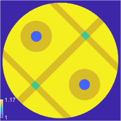
Figure 7: RI of the sample in the simulated experiment. The contrast is $35.5\%$.

For the reconstruction, we considered two different grids: $N=256^{2}$ with square pixel of length $1.76\times 10^{-2}\lambda$ and $N=512^{2}$ with square pixel of length $8.8\times 10^{-3}\lambda$. For the reconstructed algorithm, $250$ iterations were performed. The stepsize $\gamma$ and regularization parameter $\tau$ are summarized in Table I. Moreover, only six measurements were randomly selected to evaluate the gradient at each iteration. We define the signal-to-noise ratio (SNR) as

$$\mathrm{SNR}(\boldsymbol{\eta}^{*},\boldsymbol{\eta}_{\mathrm{true}})=20\log_{10}\frac{\|\boldsymbol{\eta}_{\mathrm{true}}\|}{\|\boldsymbol{\eta}_{\mathrm{true}}-\boldsymbol{\eta}^{*}\|}\mathrm{dB},$$ (37)

where $\boldsymbol{\eta}^{*}$ is the reconstructed RI. To compare the reconstruction on different discretizations, we computed the SNR on the finest grid ($N=1024^{2}$) by upsampling the reconstructed sample.

TABLE I: Stepsizes and regularization parameter on the simulated data for $N=256^{2}$ and $512^{2}$.

$N$	LiS		MGH
	$\gamma$	$\tau$	$\gamma$	$\tau$
$256^{2}$	$8.5\times 10^{-4}$	$3.5\times 10^{-3}$	$9\times 10^{-4}$	$4.5\times 10^{-3}$
$512^{2}$	$4.2\times 10^{-4}$	$7.3\times 10^{-3}$	$3.2\times 10^{-4}$	$9.5\times 10^{-3}$

We present in Fig. 8 the SNR and CPU time for both LiS and Helmholtz models with different grids. The fine discretization ($N=512^{2}$) yields an SNR higher than the coarser grid ($N=256^{2}$) does, which shows the influence of the discretization in the reconstruction. Moreover, our visual assessment in Fig. 9 corroborates the quantitative comparison. For the LiS method, Bi-CGSTAB needs only about twenty iterations to converge because the contrast is mildly hard. We still observe that the Helmholtz method needs less CPU time than the LiS method for $N=256^{2}$. For $N=512^{2}$, we see that the Helmholtz method is faster than the LiS method, which illustrates well the advantage of our method for large $N$.

Figure 8: SNR (top) and CPU time (bottom) with the simulated data for $N=256^{2}$ and $512^{2}$.

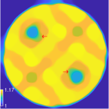
(a) LiS: $N=256^{2}$.

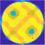
(b) MGH: $N=256^{2}$.

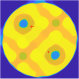
(c) LiS: $N=512^{2}$.

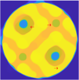
(d) MGH: $N=512^{2}$.

Figure 9: Reconstructed RIs of the object on $N=256^{2}$ and $512^{2}$ grids. All targets are upsampled to a $(1024\times 1024)$ grid.

VI-C Inverse Scattering with Experimental Data

Now, we study the performance of the Helmholtz model to recover the RIs of three real targets (namely FoamDielExtTM, FoamDielintTM, and FoamTwinDielTM) from the public database provided by the Fresnel Institute [53]. The samples are fully enclosed in a square domain of length $15$cm. We discretized the domain over a $(256\times 256)$ grid in our reconstruction. The sensors were placed circularly around the object at a distance of $1.67$m from its center with a total of $360$ sensors. Eight (eighteen, respectively) sources for FoamDielExtTM and FoamDielintTM (FoamTwinDielTM, respectively) were put uniformly around the object and activated sequentially. For each activated source, only the $241$ farthest sensors were activated. In total, $(8\times 241)$ ($(18\times 241)$, respectively) measurements for the FoamDielExtTM and FoamDielintTM (FoamTwinDielTM, respectively) targets were obtained. We used four frequencies of illumination ($3,5,6,8$GHz) to reconstruct the samples, resulting in a total of $(4\times 8\times 241)$ measurements ($(4\times 18\times 241)$ measurements for FoamTwinDielTM). The expected RIs of the three samples are presented in Fig. 10 as reference.

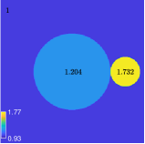
(a) FoamDielExtTM

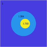
(b) FoamDielintTM

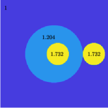
(c) FoamTwinDielTM

Figure 10: RIs of three real targets in the Fresnel database.

For the reconstruction, we randomly selected a fourth of the measurements to evaluate the gradient at each iteration and performed $150$ iterations. The stepsize and regularization parameter are summarized in Table II. From Figs. 11, 12 and 13, we see that both the LiS and Helmholtz models successfully recover the RIs of real targets with similar performance. Moreover, we observe that the Helmholtz model with the proposed MG solver is faster than the LiS model for all three targets, thus demonstrating the efficiency of our method.

TABLE II: Stepsizes and regularization parameter on the experimental data for $N=256^{2}$.

Target LiS MGH $\gamma$ $\tau$ $\gamma$ $\tau$ FoamDielExtTM $4\times 10^{-4}$ $9\times 10^{-3}$ $1.1\times 10^{-3}$ $8.1\times 10^{-3}$ FoamDielintTM $4\times 10^{-4}$ $1.9\times 10^{-2}$ $1\times 10^{-3}$ $7\times 10^{-3}$ FoamTwinDielTM $3\times 10^{-4}$ $1\times 10^{-2}$ $7\times 10^{-4}$ $7.5\times 10^{-3}$

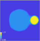
(a) LiS SNR: $26.95$dB.

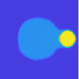
(b) MGH SNR: $26.72$dB.

Figure 11: Reconstruction of the LiS and Helmholtz models for the FoamDielExtTM target.

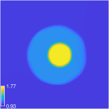
(a) LiS SNR: $27.99$dB.

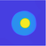
(b) MGH SNR: $28.04$dB.

Figure 12: Reconstruction of the LiS and Helmholtz models for the FoamDielintTM target.

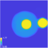
(a) LiS SNR: $22.14$dB.

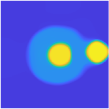
(b) MGH SNR: $22.3$dB.

Figure 13: Reconstruction of the LiS and Helmholtz models for the FoamTwinDielTM target.

VII Conclusions

We have proposed an effective and robust multigrid solver for the Helmholtz equation. We have shown that our method is adequate and efficient for diffraction tomography, especially for strongly scattering samples. This contrasts with Lippmann-Schwinger (LiS) methods which suffer from slow convergence for such challenging cases. Moreover, the proposed Jacobian matrix for the Helmholtz model is efficiently computed as well. For future works, we plan to extend the Helmholtz model to the three-dimensional case, which presents some additional challenges as in the case of LiS.

References

- [1] E. Wolf, “Three-dimensional structure determination of semi-transparent objects from holographic data,” Optics Communications, vol. 1, no. 4, pp. 153–156, 1969.
- [2] D. Jin, R. Zhou, Z. Yaqoob, and P. T. So, “Tomographic phase microscopy: principles and applications in bioimaging,” JOSA B, vol. 34, no. 5, pp. B64–B77, 2017.
- [3] A. Devaney, “Inverse-scattering theory within the Rytov approximation,” Optics Letters, vol. 6, no. 8, pp. 374–376, 1981.
- [4] Y. Sung, W. Choi, C. Fang-Yen, K. Badizadegan, R. R. Dasari, and M. S. Feld, “Optical diffraction tomography for high resolution live cell imaging,” Optics Express, vol. 17, no. 1, pp. 266–277, 2009.
- [5] J. Lim, K. Lee, K. H. Jin, S. Shin, S. Lee, Y. Park, and J. C. Ye, “Comparative study of iterative reconstruction algorithms for missing cone problems in optical diffraction tomography,” Optics Express, vol. 23, no. 13, pp. 16 933–16 948, 2015.
- [6] F. Yang, T.-a. Pham, H. Gupta, M. Unser, and J. Ma, “Deep-learning projector for optical diffraction tomography,” Optics Express, vol. 28, no. 3, pp. 3905–3921, 2020.
- [7] A. Dubois, K. Belkebir, and M. Saillard, “Retrieval of inhomogeneous targets from experimental frequency diversity data,” Inverse Problems, vol. 21, no. 6, p. S65, 2005.
- [8] P. C. Chaumet and K. Belkebir, “Three-dimensional reconstruction from real data using a conjugate gradient-coupled dipole method,” Inverse Problems, vol. 25, no. 2, p. 024003, 2009.
- [9] E. Mudry, P. C. Chaumet, K. Belkebir, and A. Sentenac, “Electromagnetic wave imaging of three-dimensional targets using a hybrid iterative inversion method,” Inverse Problems, vol. 28, no. 6, p. 065007, 2012.
- [10] U. S. Kamilov, I. N. Papadopoulos, M. H. Shoreh, A. Goy, C. Vonesch, M. Unser, and D. Psaltis, “Learning approach to optical tomography,” Optica, vol. 2, no. 6, pp. 517–522, 2015.
- [11] ——, “Optical tomographic image reconstruction based on beam propagation and sparse regularization,” IEEE Transactions on Computational Imaging, vol. 2, no. 1, pp. 59–70, 2016.
- [12] J. Lim, A. Goy, M. H. Shoreh, M. Unser, and D. Psaltis, “Learning tomography assessed using Mie theory,” Physical Review Applied, vol. 9, no. 3, p. 034027, 2018.
- [13] J. Lim, A. B. Ayoub, E. E. Antoine, and D. Psaltis, “High-fidelity optical diffraction tomography of multiple scattering samples,” Light: Science & Applications, vol. 8, no. 1, p. 82, 2019.
- [14] H.-Y. Liu, D. Liu, H. Mansour, P. T. Boufounos, L. Waller, and U. S. Kamilov, “SEAGLE: Sparsity-driven image reconstruction under multiple scattering,” IEEE Transactions on Computational Imaging, vol. 4, no. 1, pp. 73–86, 2017.
- [15] E. Soubies, T.-a. Pham, and M. Unser, “Efficient inversion of multiple-scattering model for optical diffraction tomography,” Optics Express, vol. 25, no. 18, pp. 21 786–21 800, 2017.
- [16] T.-a. Pham, E. Soubies, A. Ayoub, J. Lim, D. Psaltis, and M. Unser, “Three-dimensional optical diffraction tomography with Lippmann-Schwinger model,” IEEE Transactions on Computational Imaging, vol. 6, pp. 727–738, 2020.
- [17] A. Kadu, H. Mansour, and P. T. Boufounos, “High-contrast reflection tomography with total-variation constraints,” IEEE Transactions on Computational Imaging, vol. 6, pp. 1523–1536, 2020.
- [18] B. T. Draine and P. J. Flatau, “Discrete-dipole approximation for scattering calculations,” Journal of the Optical Society of America A, vol. 11, no. 4, pp. 1491–1499, 1994.
- [19] J. Girard, G. Maire, H. Giovannini, A. Talneau, K. Belkebir, P. C. Chaumet, and A. Sentenac, “Nanometric resolution using far-field optical tomographic microscopy in the multiple scattering regime,” Physical Review A, vol. 82, no. 6, p. 061801, 2010.
- [20] T. Zhang, C. Godavarthi, P. C. Chaumet, G. Maire, H. Giovannini, A. Talneau, M. Allain, K. Belkebir, and A. Sentenac, “Far-field diffraction microscopy at /10 resolution,” Optica, vol. 3, no. 6, pp. 609–612, 2016.
- [21] L. Ying, “Sparsifying preconditioner for the Lippmann–Schwinger equation,” Multiscale Modeling & Simulation, vol. 13, no. 2, pp. 644–660, 2015.
- [22] F. Liu and L. Ying, “Sparsify and sweep: An efficient preconditioner for the Lippmann–Schwinger equation,” SIAM Journal on Scientific Computing, vol. 40, no. 2, pp. B379–B404, 2018.
- [23] A. Sommerfeld, Partial Differential Equations in Physics. Academic Press, 1949.
- [24] J. A. Schmalz, G. Schmalz, T. E. Gureyev, and K. M. Pavlov, “On the derivation of the Green’s function for the Helmholtz equation using generalized functions,” American Journal of Physics, vol. 78, no. 2, pp. 181–186, 2010.
- [25] H. A. Van der Vorst, “Bi-CGSTAB: A fast and smoothly converging variant of bi-CG for the solution of nonsymmetric linear systems,” SIAM Journal on Scientific and Statistical Computing, vol. 13, no. 2, pp. 631–644, 1992.
- [26] G. Vainikko, “Fast solvers of the lippmann-schwinger equation,” in Direct and Inverse Problems of Mathematical Physics, R. P. Gilbert, J. Kajiwara, and Y. S. Xu, Eds. Boston, MA: Springer US, 2000, pp. 423–440. [Online]. Available: https://doi.org/10.1007/978-1-4757-3214-6_25
- [27] F. Vico, L. Greengard, and M. Ferrando, “Fast convolution with free-space green’s functions,” Journal of Computational Physics, vol. 323, pp. 191–203, 2016. [Online]. Available: https://www.sciencedirect.com/science/article/pii/S0021999116303230
- [28] A. Brandt, “Multi-level adaptive solutions to boundary-value problems,” Mathematics of Computation, vol. 31, no. 138, pp. 333–390, 1977.
- [29] ——, “Rigorous quantitative analysis of multigrid, i. Constant coefficients two-level cycle with -norm,” SIAM Journal on Numerical Analysis, vol. 31, no. 6, pp. 1695–1730, 1994.
- [30] U. Trottenberg, C. W. Oosterlee, and A. Schuller, Multigrid. Academic Press, 2000.
- [31] J. Xu and L. Zikatanov, “Algebraic multigrid methods,” Acta Numerica, vol. 26, pp. 591–721, 2017.
- [32] W. L. Briggs, V. E. Henson, and S. F. McCormick, A Multigrid Tutorial, Second Edition, 2nd ed. Society for Industrial and Applied Mathematics, 2000. [Online]. Available: https://epubs.siam.org/doi/abs/10.1137/1.9780898719505
- [33] H. C. Elman, O. G. Ernst, and D. P. O’leary, “A multigrid method enhanced by Krylov subspace iteration for discrete Helmholtz equations,” SIAM Journal on Scientific Computing, vol. 23, no. 4, pp. 1291–1315, 2001.
- [34] O. G. Ernst and M. J. Gander, “Why it is difficult to solve Helmholtz problems with classical iterative methods,” in Numerical Analysis of Multiscale Problems, I. G. Graham, T. Y. Hou, O. Lakkis, and R. Scheichl, Eds. Berlin, Heidelberg: Springer Berlin Heidelberg, 2012, pp. 325–363. [Online]. Available: https://doi.org/10.1007/978-3-642-22061-6_10
- [35] R. Wienands and W. Joppich, Practical Fourier Analysis for Multigrid Methods. Chapman and Hall/CRC, 2004.
- [36] I. Yavneh, “Coarse-grid correction for nonelliptic and singular perturbation problems,” SIAM Journal on Scientific Computing, vol. 19, no. 5, pp. 1682–1699, 1998.
- [37] A. Brandt and I. Livshits, “Wave-ray multigrid method for standing wave equations.” ETNA. Electronic Transactions on Numerical Analysis [electronic only], vol. 6, pp. 162–181, 1997. [Online]. Available: http://eudml.org/doc/119506
- [38] C. C. Stolk, M. Ahmed, and S. K. Bhowmik, “A multigrid method for the Helmholtz equation with optimized coarse grid corrections,” SIAM Journal on Scientific Computing, vol. 36, no. 6, pp. A2819–A2841, 2014.
- [39] Y. A. Erlangga, C. W. Oosterlee, and C. Vuik, “A novel multigrid based preconditioner for heterogeneous Helmholtz problems,” SIAM Journal on Scientific Computing, vol. 27, no. 4, pp. 1471–1492, 2006.
- [40] H. Calandra, S. Gratton, X. Pinel, and X. Vasseur, “An improved two-grid preconditioner for the solution of three-dimensional Helmholtz problems in heterogeneous media,” Numerical Linear Algebra with Applications, vol. 20, no. 4, pp. 663–688, 2013.
- [41] E. Treister and E. Haber, “A multigrid solver to the Helmholtz equation with a point source based on travel time and amplitude,” Numerical Linear Algebra with Applications, vol. 26, no. 1, p. e2206, 2019.
- [42] L. I. Rudin, S. Osher, and E. Fatemi, “Nonlinear total variation based noise removal algorithms,” Physica D: Nonlinear Phenomena, vol. 60, no. 1, pp. 259–268, 1992. [Online]. Available: https://www.sciencedirect.com/science/article/pii/016727899290242F
- [43] S. Lefkimmiatis, J. P. Ward, and M. Unser, “Hessian Schatten-norm regularization for linear inverse problems,” IEEE Transactions on Image Processing, vol. 22, no. 5, pp. 1873–1888, 2013.
- [44] U. S. Kamilov, H. Mansour, and B. Wohlberg, “A plug-and-play priors approach for solving nonlinear imaging inverse problems,” IEEE Signal Processing Letters, vol. 24, no. 12, pp. 1872–1876, 2017.
- [45] T. Hong, I. Yavneh, and M. Zibulevsky, “Solving RED with weighted proximal methods,” IEEE Signal Processing Letters, vol. 27, pp. 501–505, 2020.
- [46] T.-a. Pham, E. Soubies, A. Ayoub, D. Psaltis, and M. Unser, “Adaptive regularization for three-dimensional optical diffraction tomography,” in Proceedings of the Seventeenth IEEE International Symposium on Biomedical Imaging (ISBI’20), Iowa City IA, USA, April 5-7, 2020, pp. 182–186.
- [47] A. Beck and M. Teboulle, “A fast iterative shrinkage-thresholding algorithm for linear inverse problems,” SIAM Journal on Imaging Sciences, vol. 2, no. 1, pp. 183–202, 2009.
- [48] Y. Nesterov, “Gradient methods for minimizing composite functions,” Mathematical Programming, vol. 140, no. 1, pp. 125–161, 2013.
- [49] A. Beck and M. Teboulle, “Fast gradient-based algorithms for constrained total variation image denoising and deblurring problems,” IEEE Transactions on Image Processing, vol. 18, no. 11, pp. 2419–2434, 2009.
- [50] E. Soubies, F. Soulez, M. T. McCann, T.-a. Pham, L. Donati, T. Debarre, D. Sage, and M. Unser, “Pocket guide to solve inverse problems with GlobalBioIm,” Inverse Problems, vol. 35, no. 10, p. 104006, 2019.
- [51] H. Knibbe, C. W. Oosterlee, and C. Vuik, “GPU implementation of a Helmholtz Krylov solver preconditioned by a shifted Laplace multigrid method,” Journal of Computational and Applied Mathematics, vol. 236, no. 3, pp. 281–293, 2011.
- [52] A. J. Devaney, Mathematical Foundations of Imaging, Tomography and Wavefield Inversion. Cambridge University Press, 2012.
- [53] J.-M. Geffrin, P. Sabouroux, and C. Eyraud, “Free space experimental scattering database continuation: Experimental set-up and measurement precision,” Inverse Problems, vol. 21, no. 6, p. S117, 2005.