Inference and forecasting for continuous-time integer-valued trawl processes

Abstract

This paper develops likelihood-based methods for estimation, inference, model selection, and forecasting of continuous-time integer-valued trawl processes. The full likelihood of integer-valued trawl processes is, in general, highly intractable, motivating the use of composite likelihood methods, where we consider the pairwise likelihood in lieu of the full likelihood. Maximizing the pairwise likelihood of the data yields an estimator of the parameter vector of the model, and we prove consistency and, in the short memory case, asymptotic normality of this estimator. When the underlying trawl process has long memory, the asymptotic behaviour of the estimator is more involved; we present some partial results for this case. The pairwise approach further allows us to develop probabilistic forecasting methods, which can be used to construct the predictive distribution of integer-valued time series. In a simulation study, we document the good finite sample performance of the likelihood-based estimator and the associated model selection procedure. Lastly, the methods are illustrated in an application to modelling and forecasting financial bid-ask spread data, where we find that it is beneficial to carefully model both the marginal distribution and the autocorrelation structure of the data.

Keywords: Count data; Lévy basis; pairwise likelihood; estimation; model selection; forecasting.

JEL Codes: C13; C51; C52; C53; C58.

1 Introduction

In this paper, we develop likelihood-based methods for estimation, inference, model selection, and forecasting of continuous-time integer-valued trawl (IVT) processes. IVT processes, introduced in Barndorff-Nielsen et al. (2014), are a flexible class of integer-valued, serially correlated, stationary, and infinitely divisible continuous-time stochastic processes. In general, however, IVT processes are not Markovian, which implies that the structure of the full likelihood of an IVT process is highly intractable (Shephard & Yang, 2016). This is the impetus of the present paper, where we propose to use composite likelihood (CL, Lindsay, 1988) methods for estimation and inference. Specifically, we propose to estimate the parameters of an IVT model by maximizing the pairwise likelihood of the data. CL methods in general, and the pairwise likelihood approach in particular, have been successfully used in many applications, such as statistical genetics (Larribe & Fearnhead, 2011), geostatistics (Hjort & Omre, 1994), and finance (Engle et al., 2020). See Varin et al. (2011) for an excellent overview of CL methods. Although the theory behind CL estimation is quite well understood in the case of iid observations (e.g. Cox & Reid, 2004; Varin & Vidoni, 2005), the time series case, which is what we consider here, generally requires separate treatment (Varin et al., 2011, p. 11). For instance, Davis & Yau (2011) develops the theory of CL estimators in the setting of linear Gaussian time series models, while Chen et al. (2016) and Ng et al. (2011) consider CL methods for a hidden Markov model and a time series model with a latent autoregressive process, respectively. Also, Sørensen (2019) develops a two-step CL estimation method for parameter-driven count time series models with covariates. Our paper adds to the literature on CL methods for time series models by deriving the theoretical properties (consistency, asymptotic normality) of a pairwise CL estimator applied to IVT models.

A central feature of IVT processes is that they allow for specifying the correlation structure of the model separately from the marginal distribution of the model, making them flexible and well-suited for modelling count- or integer-valued data. In particular, the marginal distribution of an IVT process can be any integer-valued infinitely divisible distribution, while the correlation structure can be specified independently using a so-called trawl function. This setup allows for both short- and long-memory of the IVT process. So far, IVT processes have been applied to financial data (Barndorff-Nielsen et al., 2014; Shephard & Yang, 2017; Veraart, 2019) and real-valued trawl processes to the modelling of extreme events in environmental time series (Noven et al., 2018). IVT processes are, under weak conditions, stationary and ergodic, which motivated Barndorff-Nielsen et al. (2014) to suggest a method-of-moments-based estimator for the parameters of the IVT model. This method-of-moments-based estimator has been used in most applied work using IVT processes (e.g. Barndorff-Nielsen et al., 2014; Shephard & Yang, 2017; Veraart, 2019). Exceptions are Shephard & Yang (2016) and Noven et al. (2018). In Noven et al. (2018), a pairwise likelihood was used for a hierarchical model involving a latent (Gamma-distributed) trawl process and the corresponding asymptotic theory was derived in Courgeau & Veraart (2021). However, the asymptotic theory for inference for integer-valued trawl processes which are observed directly is not covered by these earlier papers. In Shephard & Yang (2016), the authors derive a prediction decomposition of the likelihood function of a particularly simple IVT process, the so-called Poisson-Exponential IVT process, allowing them to conduct likelihood-based estimation and inference. Although the likelihood estimation method developed in Shephard & Yang (2016) theoretically applies to more general IVT processes, the computational burden quickly becomes overwhelming in these scenarios, making estimation by classical maximum likelihood methods infeasible in practice.

The contributions of this paper can be summarized as follows. First, we derive the theoretical mixing properties of IVT processes. Using these, we prove consistency and, in the short memory case, asymptotic normality of the maximum composite likelihood (MCL) estimator of the parameter vector of an IVT model. We discuss the long memory case and, based on a result about the asymptotic behaviour of partial sums of IVT processes, conjecture that the MCL estimator has an $\alpha$-stable limit with infinite variance in this case. For the purpose of conducting feasible inference and model selection, we propose two alternative estimators of the asymptotic variance of the MCL estimator in the short memory case: a kernel-based estimator, inspired by the heteroskedastic and autocorrelation consistent (HAC) estimator of Newey & West (1987), and a simulation-based estimator. Second, we use the same principle of considering the pairwise likelihood in lieu of the full likelihood, to derive the predictive distribution of an IVT model, conditional on the current value of the process; this allows us to use the IVT framework for forecasting integer-valued data. In a simulation study, we compare the MCL estimator to the standard method-of-moments-based estimator suggested in Barndorff-Nielsen et al. (2014) and find that the MCL estimator provides substantial improvements in most cases. Indeed, in a realistic simulation setup, we find that the MCL estimator can improve on the method-of-moments-based estimator by more than $50\%$, in terms of finite sample root median squared error. Since the asymptotic theory for (G)MM estimation of trawl processes has not been worked out elsewhere, we also derive the asymptotic theory for GMM estimation and present the results for comparison purposes in the Supplementary Material, see Section S12.

We apply the methods developed in the paper to a time series of the bid-ask spread of a financial asset. The time series behaviour of the bid-ask spread has been extensively studied in the literature on the theory of the microstructure of financial markets (e.g. Huang & Stoll, 1997; Bollen et al., 2004). The model selection procedure developed in the paper indicates that a model with Negative Binomial marginal distribution and slowly decaying autocorrelations most adequately describe the data. These findings are in line with those of Groß-KlußMann & Hautsch (2013), who also found strong persistence in bid-ask spread time series. Then, in a pseudo-out-of-sample forecast exercise, we find that it is important to carefully model both the marginal distribution and the autocorrelation structure to get accurate forecasts of the future bid-ask spread. These findings highlight the strength of modelling using a framework where the choice of marginal distribution can be made independently of the choice of autocorrelation structure.

The rest of the paper is structured as follows. Section 2 outlines the mathematical setup of IVT processes, while Section 3 contains details on the estimation and model selection procedures. Section 4 presents the theory behind our proposed forecasting approach. Section 5 summarises the results from our simulation study, investigating the finite sample properties of the estimation and model selection procedures. Section 6 illustrates the use of the new methodology in an empirical application to financial bid-ask spread data. Section 7 concludes. The proofs of the main mathematical results are given in an Appendix. Practical details on the implementation of the asymptotic theory and additional derivations are given in the Supplementary Material, which also contains further simulation results and extensive details on various calculations used in the implementation of the methods. A software package for the implementation of simulation, estimation, inference, model selection, and forecasting of IVT processes is freely available in the MATLAB programming language.

2 Integer-valued trawl processes

Let $(\Omega,\mathcal{F},\mathbb{P})$ denote a probability space, supporting a Poisson random measure $N$, defined on $\mathbb{Z}\times[0,1]\times\mathbb{R}$, with mean (intensity) measure $\eta\otimes Leb\otimes Leb$. Throughout $Leb$ denotes the Lebesgue measure and $\eta$ is a Lévy measure. A Lévy basis $L$ is a homogeneous and independently scattered random measure on $[0,1]\times\mathbb{R}$, defined as

$$L(dx,ds):=\int_{-\infty}^{\infty}yN(dy,dx,ds),\quad(x,s)\in[0,1]\times\mathbb{R}.$$ (2.1)

See, e.g., Rajput & Rosinski (1989) and Barndorff-Nielsen (2011) for further details on Lévy bases. Since we are only interested in integer-valued Lévy bases, we will work under the following assumption.

Assumption 2.1.

The Lévy basis $L$ is given by (2.1) with Lévy measure $\eta$, concentrated on the integers ($y\in\mathbb{Z}$), such that $\|\eta\|:=\sum_{y=-\infty}^{\infty}y^{2}\eta(y)<\infty$.

The Lévy basis $L$ is an infinitely divisible random measure with cumulant (log-characteristic) function

$$C_{L(dx,ds)}(\theta):=\log\mathbb{E}[\exp(i\theta L(dx,ds))]=\int_{-\infty}^{\infty}\left(e^{i\theta y}-1\right)\eta(dy)dxds,\quad(x,s)\in[0,1]\times\mathbb{R}.$$

An important random variable associated with the Lévy basis $L,$ is the so-called Lévy seed, $L^{\prime}$, which we define as the random variable $L^{\prime}$ satisfying $\mathbb{E}[\exp(i\theta L^{\prime})]=\exp(C_{L^{\prime}}(\theta)),$ with $C_{L^{\prime}}(\theta)=\sum_{y=-\infty}^{\infty}\left(e^{i\theta y}-1\right)\eta(y)$.

Remark 2.1.

Because the distribution of a Lévy process is entirely determined by its distribution at a particular time point, we can specify a Lévy process $L_{t}^{\prime}$ from a Lévy seed $L^{\prime}$, by requiring that $L_{1}^{\prime}\sim L^{\prime}$.

Using the Lévy seed, we can rewrite the cumulant function of the Lévy basis as $C_{L(dx,ds)}(\theta)=C_{L^{\prime}}(\theta)dxds$, or, for a Borel set $B\in\mathcal{B}([0,1]\times\mathbb{R}),$

$$C_{L(B)}(\theta)=C_{L^{\prime}}(\theta)Leb(B).$$ (2.2)

From (2.2) we have that $\kappa_{j}(L(B))=\kappa_{j}(L^{\prime})Leb(B)$, $j\geq 0$, where $\kappa_{j}(Z)$ denotes the $j$th cumulant of the random variable $Z$, when it exists. In particular $\mathbb{E}[L(B)]=\mathbb{E}[L^{\prime}]Leb(B)$, and $Var(L(B))=Var(L^{\prime})Leb(B)$. The relationship (2.2) implies that the distribution of the random variable $L(B)$ is entirely specified by the Lévy seed $L^{\prime}$ and the Lebesgue measure of the set $B$. In Section 2.1 below, we illustrate how this can be used to construct trawl processes with a given marginal distribution.

The Lévy basis $L$ acts on sets in $\mathcal{B}([0,1]\times\mathbb{R})$. We restrict attention to trawl sets of the form

$$A_{t}=A+(0,t),\quad A=\{(x,s):s\leq 0,0\leq x<d(s)\},\quad t\geq 0,$$ (2.3)

where $d$ is a trawl function, determining the shape of the trawl set $A_{t}$. Section 2.2 contains several parametric examples for the trawl function $d$. We will impose the following assumption.

Assumption 2.2.

The trawl set $A_{t}$ is given by (2.3), where the trawl function $d:\mathbb{R}_{-}\to[0,1]$ is continuous and monotonically increasing such that $Leb(A)=\int_{-\infty}^{0}d(s)<\infty$.

Intuitively, $A_{t}$ is obtained from the set $A$ by “dragging” it along in time. Note in particular that $Leb(A_{t})=Leb(A)$ for all $t$. Finally, define the IVT process $X=(X_{t})_{t\geq 0}$ as the Lévy basis evaluated over the trawl set:

$$X_{t}:=L(A_{t}),\quad t\geq 0.$$ (2.4)

2.1 Modelling the marginal distribution

For an IVT process $X$ as defined in (2.4), we have $C_{X_{t}}(\theta)=C_{L(A_{t})}(\theta)=Leb(A)C_{L^{\prime}}(\theta)=C_{L^{\prime}_{Leb(A)}}(\theta)$, where $L^{\prime}_{t}$ is a Lévy process with $L^{\prime}_{1}\sim L^{\prime}$. Hence we observe that the marginal distribution of the IVT process $X_{t}$ is entirely decided by the Lebesgue measure of the trawl set $A$ and the Lévy seed $L^{\prime}$ of the underlying Lévy basis $L$. Indeed, by specifying a distribution for $L^{\prime}$, we can build IVT processes with the corresponding marginal distribution. The following two examples illustrate how to do this; additional details can be found in the Supplementary Material.

Example 2.1 (Poissonian Lévy seed).

Let $L^{\prime}\sim\textnormal{Poisson}(\nu)$, i.e. $L^{\prime}$ is distributed as a Poisson random variable with intensity $\nu>0$. It follows from standard properties of the Poisson distribution that $X_{t}\sim\textnormal{Poisson}(\nu Leb(A))$. In other words, for all $t\geq 0$, $P\left(X_{t}=x\right)=(\nu Leb(A))^{x}e^{-\nu Leb(A)}/x!$, $x=0,1,2,\ldots$.

Example 2.2 (Negative Binomial Lévy seed).

Let $L^{\prime}\sim\textnormal{NB}(m,p)$, i.e. $L^{\prime}$ is distributed as a Negative Binomial random variable with parameters $m>0$ and $p\in[0,1]$. It follows from standard properties of the Negative Binomial distribution that $X_{t}\sim\textnormal{NB}(mLeb(A),p)$. In other words, for all $t\geq 0$, $P(X_{t}=x)=\frac{\Gamma(Leb(A)m+x)}{x!\Gamma(Leb(A)m)}(1-p)^{Leb(A)m}p^{x}$, $x=0,1,2,\ldots$, where $\Gamma(z)=\int_{0}^{\infty}y^{z-1}e^{-y}dy$ for $z>0$ is the $\Gamma$-function.

2.2 Modelling the correlation structure

Recall that the shape of the trawl set $A_{t}$ is determined by the trawl function $d$, see Equation (2.3). A particularly tractable and flexible class of parametrically specified trawl functions are the so-called superposition trawls (Barndorff-Nielsen et al., 2014; Shephard & Yang, 2017). They are defined as $d(s):=\int_{0}^{\infty}e^{\lambda s}\pi(d\lambda)$, for $s\leq 0$, where $\pi$ is a probability measure on $\mathbb{R}_{+}.$ This construction essentially randomizes the decay parameter $\lambda$ in an otherwise exponential function.

The IVT process with a superposition trawl function is stationary. Hence, we get the autocorrelation function (Barndorff-Nielsen et al., 2014)

$$\rho(h):=Corr(L(A_{t+h}),L(A_{t}))=\frac{Leb(A_{h}\cap A)}{Leb(A)}=\frac{\int_{h}^{\infty}d(-s)ds}{\int_{0}^{\infty}d(-s)ds},\quad h>0.$$ (2.5)

Example 2.3 (Exponential trawl function).

For the case where the measure $\pi$ has an atom at $\lambda>0,$ i.e. $\pi(dx)=\delta_{\lambda}(dx),$ where $\delta_{x}(\cdot)$ is the Dirac delta function at $x\in\mathbb{R}_{+},$ we get $d(s)=e^{\lambda s}$ for $s\leq 0$. Consequently, $\rho(h)=\exp(-\lambda h)$, for $h\geq 0$.

Example 2.4 (Inverse Gaussian trawl function).

Letting $\pi$ be given by the inverse Gaussian distribution $\pi(dx)=\frac{(\gamma/\delta)^{1/2}}{2K_{1/2}(\delta\gamma)}x^{-1/2}\exp\left(-\frac{1}{2}(\delta^{2}x^{-1}+\gamma^{2}x)\right)dx$, where $K_{\nu}(\cdot)$ is the modified Bessel function of the third kind and $\gamma,\delta\geq 0$ with both not zero simultaneously. It can be shown that the resulting trawl function is given by $d(s)=\left(1-\frac{2s}{\gamma^{2}}\right)^{-1/2}\exp\left(\delta\gamma\left(1-\sqrt{1-\frac{2s}{\gamma^{2}}}\right)\right)$, for $s\leq 0$, and hence that the correlation function of the IVT process with inverse Gaussian trawl function becomes $\rho(h)=Corr(X_{t+h},X_{t})=\exp\left(-\delta\gamma(\sqrt{1+2h/\gamma^{2}}-1)\right)$, for $h\geq 0$. The details on these calculations can be found in the Supplementary Material.

Example 2.5 (Gamma trawl function).

Let $\pi$ have the $\Gamma(1+H,\alpha)$ density, $\pi(dx)=\frac{1}{\Gamma(1+H)}\alpha^{1+H}\lambda^{H}e^{-\lambda\alpha}dx$, where $\alpha>0$ and $H>0.$ We can show that $d(s)=\left(1-\frac{s}{\alpha}\right)^{-(H+1)}$, $s\leq 0$, which implies the correlation function $\rho(h)=Corr(X_{t+h},X_{t})=\frac{Leb(A_{h}\cap A)}{Leb(A)}=\left(1+\frac{h}{\alpha}\right)^{-H}$. Note that in this case $\int_{0}^{\infty}\rho(h)dh=\infty$ for $H\in(0,1]$ and $\int_{0}^{\infty}\rho(h)dh=\alpha(H-1)^{-1}$ for $H>1$, from which we see that an IVT process with a Gamma trawl function enjoys the long memory property, in the sense of a non-integrable autocorrelation function, when $H\in(0,1].$ The details on these calculations can be found in the Supplementary Material.

2.3 Modelling IVT processes

Using the above methods, we can build flexible continuous-time integer-valued processes with a marginal distribution determined by the underlying Lévy basis, and independently specified correlation structure determined by the trawl function. In our main examples given above, we considered a Lévy basis with Poisson or Negative Binomial marginals, and various trawl functions, namely the Exponential trawl function, the IG trawl function, and the Gamma trawl function. Other specifications for the underlying Lévy basis and trawl function than those given here could of course be considered. In practice, these choices should be guided by the properties of the data being modelled.

The simplest IVT process we can construct in this way is the Poisson-Exponential IVT process, i.e., the case where $L^{\prime}\sim\textnormal{Poisson}(\nu)$ and $d(s)=\exp(\lambda s)$, $s\leq 0$, see Examples 2.1 and 2.3. This special case results in a Markovian process, which is not in general true of IVT processes (Barndorff-Nielsen et al., 2014). In fact, the model is similar to the popular Poissonian INAR(1) model, introduced in McKenzie (1985) and Al-Osh & Alzaid (1987). An illustration of the exponential trawl set, $A_{t},$ dragged through time, together with a simulation of the resulting Poisson-Exponential IVT trawl process $X_{t}=L(A_{t})$, is seen in Figure 1. The parameters used are $\lambda=1$ and $\nu=5$. At each time point $t$, the value of $X_{t}$ (bottom plot) is the number of points inside the trawl set $A_{t}$ (top plot).

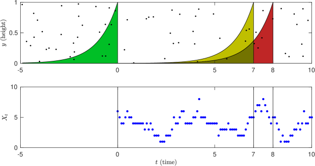
Figure 1: Top: Simulation of a Poisson Lévy basis on $\mathbb{R}\times[0,1]$ (black dots) with an exponential trawl set $A_{t}$ (shaded) superimposed at three periods in time, $t\in\{0,7,8\}$. Bottom: The associated trawl process $X_{t}=L(A_{t})$, given by the number of ‘points’ inside the trawl set $A_{t}$ at time $t$. The intensity of the Poisson random measure is $\|\eta\|=\eta(1)=\nu=5$ and the parameter controlling the exponential trawl function, $d(s)=\exp(\lambda s)$, is $\lambda=1.$

3 Estimation of integer-valued trawl processes

Barndorff-Nielsen et al. (2014) showed that the parameter vector $\theta$ of an IVT process can be consistently estimated using a generalized method of moments (GMM) procedure. In Section 3.1, we propose a likelihood-based approach instead. Both estimation procedures rely on the fact that the IVT process is stationary and mixing. The mixing property of IVT processes is obtained from results given in Fuchs & Stelzer (2013), see Barndorff-Nielsen et al. (2014, p. 699). Although mixing, in general, is sufficient for the consistency of the estimators, the central limit theorem for the likelihood-based estimator (Theorem 3.3 below) relies on the stronger mixing concept of $\alpha$-mixing, where the size (or rate) of mixing can also be established. Let us recall the definition of $\alpha$-mixing for a stationary process. Let $\mathcal{F}_{-\infty}^{0}=\sigma(X_{t};t\leq 0)$ and, for $m>0$, $\mathcal{F}_{m}^{\infty}=\sigma(X_{t};t\geq m)$, and define the numbers $\alpha_{m}:=\sup_{G\in\mathcal{F}_{-\infty}^{0},H\in\mathcal{F}_{m}^{\infty}}|\mathbb{P}(H\cap G)-\mathbb{P}(H)\mathbb{P}(G)|$, for $m>0$. The process $X=(X_{t})_{t\in\mathbb{R}}$ is $\alpha$-mixing if $\alpha_{m}\rightarrow 0$ as $m\rightarrow\infty$. It is $\alpha$-mixing of size $-\phi_{0}$ if $\alpha_{m}=O(m^{-\phi})$, as $m\rightarrow\infty$, for some $\phi>\phi_{0}$.

We obtain the following important property for IVT processes.

Theorem 3.1.

Let the IVT process $X$ be given by (2.4) and let Assumptions 2.1 and 2.2 hold. Now, $X$ is $\alpha$-mixing with $\alpha_{m}=O(\rho(m))$ as $m\rightarrow\infty$, where $\rho(m)$ is the autocorrelation function of $X$.

Remark 3.1.

The autocorrelation functions of the Exponential (Example 2.3) and IG (Example 2.4) IVT models imply that these models are in fact $\alpha$-mixing with an exponential decay rate. The autocorrelation function of the Gamma (Example 2.5) IVT model implies that it is $\alpha$-mixing of size $-(H-\epsilon)$ for all $\epsilon>0$.

Remark 3.2.

As an alternative to the proof of Theorem 3.1 provided in Appendix A, we could first show that trawl processes are $\theta$-weakly dependent, which we do in the Supplementary Material, see Section S12. Then, as pointed out in Curato & Stelzer (2019, p. 324) and shown in the discrete-time case in Doukhan et al. (2012), for integer-valued trawl processes, the fact that they are $\theta$-weakly dependent, implies that they are strongly mixing with the coefficient as stated in Theorem 3.1.

3.1 Estimation by composite likelihoods

Due to the non-Markovianity of the IVT process, we face computational difficulties when attempting to estimate the model by maximizing the full likelihood, hence we propose to use the CL method instead. The main idea behind the CL approach is to consider a, possibly misspecified, likelihood function which captures the salient features of the data at hand; here this means capturing the features of the Lévy basis, controlling the marginal distribution, and those of the trawl function, controlling the dependence structure. We focus on pairwise CLs.

3.1.1 Pairwise composite likelihood

Suppose we have $n\in\mathbb{N}$ observations of the IVT process $X,$ $x_{1},\ldots,x_{n},$ on an equidistant grid of size $\Delta=T/n$, for some $T>0$. Define the following likelihood function using pairs of observations $k$ periods apart,

$$CL^{(k)}(\theta;x):=\prod_{i=1}^{n-k}f(x_{i+k},x_{i};\theta),\quad k\geq 1,$$ (3.1)

where $f(x_{i+k},x_{i};\theta)$ is the joint probability mass function (PMF) of the observations $x_{i}$ and $x_{i+k}$, parametrized by the vector $\theta$. From (3.1), we construct the composite likelihood function

$$\mathcal{L}_{CL}(\theta;x):=\mathcal{L}_{CL}^{(K)}(\theta;x):=\prod_{k=1}^{K}CL^{(k)}(\theta;x)=\prod_{k=1}^{K}\prod_{i=1}^{n-k}f(x_{i+k},x_{i};\theta),$$ (3.2)

where $K\in\mathbb{N}$ denotes the number of pairwise likelihoods to include in the calculation of the composite likelihood function.

The maximum composite likelihood (MCL) estimator of $\theta$ is defined as

$$\hat{\theta}^{CL}:=\arg\max_{\theta\in\Theta}l_{CL}(\theta;x),$$ (3.3)

where $\Theta$ is the parameter space and $l_{CL}(\theta;x):=\log\mathcal{L}_{CL}(\theta;x)$ is the log composite likelihood function. To apply this estimator in practice, we need to be able to calculate the PMFs $f(x_{i+k},x_{i})$. Section S5 in the Supplementary Material contains a discussion on how to do this in the general integer-valued case. In the count-valued case, $f(x_{i+k},x_{i})$ takes a particularly simple form which is convenient in implementations. Indeed, letting $\mathbb{P}_{\theta}(B)$ denote the probability of the event $B$ given parameters $\theta$, we have the following.

Proposition 3.1.

Let the IVT process $X$ be given by (2.4) and let Assumptions 2.1 and 2.2 hold. Suppose further, that the Lévy basis $L$ is non-negative, i.e. $\eta(y)=0$ for $y<0$. The joint PMF of two observations $x_{i+k}$ and $x_{i}$ is

$$f(x_{i+k},x_{i};\theta)=\sum_{c=0}^{\min\{x_{i+k},x_{i}\}} \mathbb{P}_{\theta}\left(L(A_{(i+k)\Delta}\setminus A_{i\Delta})=x_{i+k}-c\right)\mathbb{P}_{\theta}\left(L(A_{i\Delta}\setminus A_{(i+k)\Delta})=x_{i}-c\right)$$

$$\cdot\mathbb{P}_{\theta}\left(L(A_{(i+k)\Delta}\cap A_{i\Delta})=c\right).$$ (3.4)

The probabilities $\mathbb{P}_{\theta}(\cdot)$ in (3.4) can be expressed as a function of the parameters of the Lévy seed and the trawl function. Indeed, for a Borel set $B\in\mathcal{B}([0,1]\times\mathbb{R})$ we have $\mathbb{P}_{\theta}(L(B)=x)=\mathbb{P}_{\theta}(L^{\prime}_{Leb(B)}=x)$, where $L^{\prime}_{t}$ is a Lévy process with $L_{1}^{\prime}\sim L^{\prime}$, and $L^{\prime}$ being the Lévy seed associated to $X$, see Remark 2.1. Also, $Leb(A_{(i+k)\Delta}\cap A_{i\Delta})=\int_{-\infty}^{-k\Delta}d(s)ds$, and $Leb(A_{(i+k)\Delta}\setminus A_{i\Delta})=Leb(A_{i\Delta}\setminus A_{(i+k)\Delta})=Leb(A)-Leb(A_{(i+k)\Delta}\cap A_{i\Delta})=\int_{-k\Delta}^{0}d(s)ds$. Plugging these into (3.4) we obtain the pairwise likelihoods, $f(x_{i+k},x_{i};\theta)$, and thus the CL function, $\mathcal{L}_{CL}(\theta;x)$, as a function of $\theta$.

Example 3.1 (Poisson-Exponential IVT process).

Let $L^{\prime}\sim\textnormal{Poisson}(\nu)$ and $d(s)=\exp(\lambda s)$, $s\leq 0$, for some $\nu,\lambda>0$. Since $L^{\prime}\sim\textnormal{Poisson}(\nu)$ we have $L(B)\sim\textnormal{Poisson}(Leb(B)\nu)$ for Borel sets $B$ and hence $\mathbb{P}_{\theta}\left(L(B)=x\right)=(\nu Leb(B))^{x}e^{-\nu Leb(B)}/x!$, for $x\geq 0$. Further, it is not difficult to show that $Leb(A_{(i+k)\Delta}\cap A_{i\Delta})=\lambda^{-1}e^{-\lambda k\Delta}$ and $Leb(A_{(i+k)\Delta}\setminus A_{i\Delta})=\lambda^{-1}(1-e^{-\lambda k\Delta})$. Using this, the probabilities in (3.4) can be expressed as functions of $\nu$ and $\lambda$ and hence the maximization (3.3) can be carried out using standard numerical methods.

3.1.2 Asymptotic theory

Because we are only considering dependencies across pairs of observations and not their dependence with the remaining observations, the pairwise composite likelihood function (3.2) can be viewed as a misspecified likelihood. Nonetheless, since the individual PMFs $f(x_{i+k},x_{i};\theta)$ in (3.2) are proper bivariate PMFs, the composite score function $\partial l_{CL}(\theta;x)/\partial\theta$ provides unbiased estimating equations and, under certain regularity assumptions, the usual asymptotic results will apply (Cox & Reid, 2004). However, as pointed out in Varin et al. (2011), formally proving the results in the time series case requires more rigorous treatment. The following two theorems provide the details on the asymptotic theory in the setup of this paper. We will work under the following identification assumption.

Assumption 3.1.

For all $\theta\in\Theta$, it holds that

$$\theta\neq\theta_{0}\Rightarrow\sum_{k=1}^{K}f(x_{1},x_{2};\theta)\neq\sum_{k=1}^{K}f(x_{1},x_{2};\theta_{0})$$ (3.5)

for some $x_{1},x_{2}\in\mathbb{Z}$.

First, we have a Law of Large Numbers.

Theorem 3.2.

Fix $K\in\mathbb{N}$, let the IVT process $X$ be given by (2.4), and let Assumptions 2.1–2.2 and 3.1 hold. Then $\hat{\theta}_{CL}\stackrel{{\scriptstyle\mathbb{P}}}{{\rightarrow}}\theta_{0}$, as $n\rightarrow\infty$.

Remark 3.3.

As is often the case, the identification condition in Assumption 3.1 can be difficult to check in practice. For the IVT processes considered in this paper and presented in the examples above, our numerical experiments indicate that requiring $K\geq\textnormal{dim}(\theta_{d})$, where $\textnormal{dim}(\theta_{d})$ denotes the dimension of the parameters controlling the trawl function $d$, results in $\theta_{0}$ being identified. A similar requirement was suggested in Davis & Yau (2011).

We also impose a standard assumption on the parameter space.

Assumption 3.2.

The set $\Theta$ is compact such that the true parameter vector, $\theta_{0}$, lies in the interior of $\Theta$.

It turns out that the asymptotic behaviour of the MCL estimator differs in the short- and long-memory cases. The former is captured by the following assumption.

Assumption 3.3 (Short memory).

The autocorrelation function of the IVT process satisfies $\lim_{n\rightarrow\infty}\rho(n)n=0$.

Remark 3.4.

Assumption 3.3 is satisfied by IVT processes with the Exponential trawl (Example 2.3), the Inverse Gaussian trawl (Example 2.4), and the Gamma trawl (Example 2.5) with $H>1$.

Under this assumption, the mixing property of IVT processes, presented in Theorem 3.1, implies that we can invoke a Central Limit Theorem for triangular arrays of mixing processes (Davidson, 1994, Corollary 24.7) to get the following result.

Theorem 3.3.

Let the conditions from Theorem 3.2 hold, together with Assumptions 3.2–3.3. Then,

$$\sqrt{n}(\hat{\theta}^{CL}-\theta_{0})\stackrel{{\scriptstyle d}}{{\rightarrow}}N\left(0,G(\theta_{0})^{-1}\right),\quad n\rightarrow\infty,$$

where $G(\theta_{0})$ is the Godambe information matrix (Godambe, 1960) matrix with inverse $G(\theta_{0})^{-1}=H(\theta_{0})^{-1}V(\theta_{0})H(\theta_{0})^{-1}$, where

$$H(\theta_{0})= -\sum_{k=1}^{K}\mathbb{E}\left[\frac{\partial^{2}}{\partial\theta^{\prime}\partial\theta}\log f(X_{k\Delta},X_{0};\theta)|_{\theta=\theta_{0}}\right],\quad\mathrm{and}$$

$$V(\theta_{0})= \sum_{k=1}^{K}Var\left(\frac{\partial}{\partial\theta}\log f(X_{k\Delta},X_{0};\theta)|_{\theta=\theta_{0}}\right)$$

$$+2\sum_{k=1}^{K}\sum_{k^{\prime}=1}^{K}\sum_{i=1}^{\infty}Cov\left(\frac{\partial}{\partial\theta}\log f(X_{k\Delta},X_{0};\theta)|_{\theta=\theta_{0}},\frac{\partial}{\partial\theta^{\prime}}\log f(X_{(i+k^{\prime})\Delta},X_{i\Delta};\theta)|_{\theta=\theta_{0}}\right).$$

Further, the infinite sum in the expression for $V(\theta_{0})$ converges.

Theorem 3.3 implies that feasible inference can be conducted using an estimate of the inverse of the Godambe information matrix $\hat{G}(\hat{\theta}^{CL})^{-1}=\hat{H}(\hat{\theta}^{CL})^{-1}\hat{V}(\hat{\theta}^{CL})\hat{H}(\hat{\theta}^{CL})^{-1}$, where $\hat{\theta}^{CL}$ is the MCL estimate from (3.3). Note that while the straight-forward estimator $\hat{H}(\hat{\theta}^{CL})=-n^{-1}\frac{\partial}{\partial\theta\partial\theta^{\prime}}l_{CL}(\hat{\theta}^{CL};x)$ is consistent for $H(\theta)$ due to the stationarity and ergodicity of the IVT process, $\hat{V}(\hat{\theta}^{CL})$ is more difficult to obtain, since the obvious candidate $n^{-1}\frac{\partial}{\partial\theta}l_{CL}(\theta;x)\frac{\partial}{\partial\theta}l_{CL}(\theta;x)^{\prime}$ vanishes at $\theta=\hat{\theta}^{CL}$, a fact also remarked in Varin & Vidoni (2005). While it is possible to estimate $V(\theta_{0})$ using a Newey-West-type kernel estimator (Newey & West, 1987), we obtained more precise results using a simulation-based approach to estimating $V(\theta_{0})$. The details of both approaches are provided in the Supplementary Material, Section S4.

3.1.3 Asymptotic theory in the long memory case

While the consistency result in Theorem 3.2 applies for all IVT processes satisfying Assumptions 2.1–2.2 and 3.1, Assumption 3.3, required in the central limit result in Theorem 3.3, excludes IVT processes with long memory, e.g. those with autocorrelation function adhering to $\rho(h)=O(h^{-H})$ for $H\in(0,1]$. As mentioned in Remark 3.1, this is for instance the case for the Gamma trawl function (Example 2.5) with $H\in(0,1]$.

Although a long memory CLT as such eludes us, we can say some things about the asymptotic behaviour of the MCL estimator $\hat{\theta}^{CL}$ in the long memory case. For instance, the convergence rate is likely slower than $\sqrt{n}$, as the following result suggests.

Theorem 3.4.

Let the conditions from Theorem 3.2 hold and assume that the autocorrelation function of the IVT process satisfies $\rho(h)=L_{\infty}(h)h^{-H}$ for some $H\in(0,1]$, where $L_{\infty}$ is a function which is slowly varying at infinity, i.e. for all $a>0$ it holds that $\lim_{x\rightarrow\infty}\frac{L_{\infty}(ax)}{L_{\infty}(x)}=1$. Then,

1. For all $\epsilon>0$, $n^{H/2-\epsilon}(\hat{\theta}^{CL}-\theta_{0})\stackrel{{\scriptstyle\mathbb{P}}}{{\rightarrow}}0$, as $n\rightarrow\infty$.

2. Let $J=\textnormal{dim}(\theta_{0})$ be the dimension of $\theta_{0}$ and denote by $\hat{\theta}^{CL}_{i}$ and $\theta_{0,i}$ the $i$th component of the vectors $\hat{\theta}^{CL}$ and $\theta_{0}$, respectively. Then, for $i=1,2,\ldots,J$, we have that for all $\epsilon>0$, $Var\left(n^{H/2+\epsilon}(\hat{\theta}^{CL}_{i}-\theta_{0,i})\right)\rightarrow\infty$, as $n\rightarrow\infty$.

Theorem 3.4(i) implies that the convergence rate of $\hat{\theta}^{CL}$ cannot be slower than $n^{H/2}$ for $H\in(0,1]$. Further, Theorem 3.4(ii) implies that if the convergence rate is faster than $n^{H/2}$ it must necessarily be the case that the limiting random variable has an infinite variance. We conjecture that $n^{H/(H+1)}(\hat{\theta}^{CL}-\theta_{0})\stackrel{{\scriptstyle(d)}}{{\rightarrow}}MY_{1+H}$ for a matrix $M$, where $Y_{\alpha}$ is an $\alpha$-stable random vector. Note that, for $H\in(0,1)$ it is the case $H/(1+H)\in(H/2,1/2)$, meaning that the conjectured convergence rate is faster than $n^{H/2}$, but slower that $\sqrt{n}$. Our reason for the conjecture has its roots in Theorem 3.5 below. First, we introduce a technical assumption on the trawl function $d$, ensuring that we are in the long memory case.

Assumption 3.4 (Long memory).

Assume that $H\in(0,1)$ and

1. $d(-x)=g_{1}(x)x^{-H-1}$, $x>0$, where $g_{1}$ is a function that is slowly varying at infinity.

2. $d^{\prime}(-x)=g_{2}(x)x^{-H-2}$, $x>0$, where $g_{2}$ is a function that is slowly varying at infinity.

Remark 3.5.

The key condition in Theorem 3.4, namely $\rho(h)=L_{\infty}(h)h^{-H}$ for some $H\in(0,1)$, is implied by Assumption 3.4.

Remark 3.6.

The Gamma trawl function (Example 2.5) fulfils Assumption 3.4 with $g_{1}(x)=\left(x^{-1}+\alpha^{-1}\right)^{-H-1}$ and $g_{2}(x)=\frac{H+1}{\alpha}\left(x^{-1}+\alpha^{-1}\right)^{-H-2}$.

Theorem 3.5.

Suppose $L^{\prime}\sim Poi(\nu)$ and that the parameters of the trawl function $d$ are known. Let the conditions from Theorem 3.2 hold, along with Assumptions 3.2 and 3.4. Then,

$$n^{H/(1+H)}(\hat{\nu}^{CL}-\nu_{0}-R_{n})\stackrel{{\scriptstyle d}}{{\rightarrow}}H(\nu_{0})^{-1}\nu_{0}^{-1}Y_{1+H},\quad n\rightarrow\infty,$$

where $H(\nu_{0})$ is given as in Theorem 3.3, $Y_{\alpha}$ is an $\alpha$-stable random variable with characteristic function

$$\phi_{Y_{\alpha}}(u):=\mathbb{E}[\exp(iuY_{\alpha})]=\exp\left(c|u|^{\alpha}\Gamma(2-\alpha)\ \left(\cos\left(\frac{\pi\alpha}{2}\right)-i\cdot\textnormal{sgn}(u)\sin\left(\frac{\pi\alpha}{2}\right)\right)\right),\quad u\in\mathbb{R},$$ (3.6)

and where $R_{n}$ is given by

$$R_{n}=H(\nu_{0})^{-1}\nu_{0}^{-1}n^{-1}S_{n}(U),$$

with $S_{n}(U):=\sum_{i=1}^{n}\left(U_{i}-\mathbb{E}[U_{i}]\right)$ denoting the de-meaned partial sum of the sequence $U=\{U_{i}\}_{i=1}^{n}$, where $U_{i}:=\sum_{k=1}^{K}g(X_{(i+k)\Delta},X_{i\Delta})$ and $g(X_{(i+k)\Delta},X_{i\Delta}):=\mathbb{E}[L(A_{(i+k)\Delta}\setminus A_{i\Delta})|X_{(i+k)\Delta},X_{i\Delta}]$.

Remark 3.7.

The asymptotic behaviour of the remainder term $R_{n}$ in Theorem 3.5 is decided by a quite general function $g$ of the pairs $(X_{i},X_{i+k})$ and one can show that similar issues arise in the more general case where $L^{\prime}$ is integer-valued and the parameters in the trawl function are estimated. The asymptotic behaviour of such general functions of the data could possibly be studied using mixing conditions for partial sums with $\alpha$-stable limits (e.g. Jakubowski, 1993) or by deriving Breuer-Major-like theorems (Breuer & Major, 1983; Nourdin et al., 2011) valid for IVT processes using Malliavin calculus for Poissonian spaces, see Basse-O’Connor et al. (2020) for a related approach. We believe that especially this latter route could be fruitful, but leave it for future work.

The proof of Theorem 3.5 relies on a result about the partial sums of the IVT process $X$, which might be of independent interest. We, therefore, state it here.

Theorem 3.6.

Suppose the Lévy basis $L$ is non-negative, i.e. $\eta(y)=0$ for $y<0$, and let the conditions from Theorem 3.2 hold, along with Assumptions 3.2 and 3.4. Then,

$$n^{-\frac{1}{1+H}}S_{n}(X)\stackrel{{\scriptstyle d}}{{\rightarrow}}Y_{1+H},\quad n\rightarrow\infty,$$

where $Y_{\alpha}$ is an $\alpha$-stable random variable with characteristic function (3.6).

Remark 3.8.

Closely related results about partial sums of trawl processes have previously been put forth in Doukhan et al. (2019) and Pakkanen et al. (2021) in the context of a discrete-time trawl process under a standard asymptotic scheme ($n\rightarrow\infty$) and in the context of a continuous-time trawl process under an infill asymptotic sampling scheme ($\delta\rightarrow 0$), respectively. In this paper, we consider $n$ observations of the continuous-time trawl process sampled on an equidistant $\delta$-grid, $X_{\delta},X_{2\delta},\ldots,X_{n\delta}$, where $\delta>0$ is fixed, and let $n\rightarrow\infty$. In this sense, our setup is closer to the one in Doukhan et al. (2019). Indeed, it can be shown that the law of $(X_{\delta},X_{2\delta},\ldots,X_{n\delta})$ is equal to the law of $(Y_{1},Y_{2},\ldots,Y_{n})$, where $Y$ is an appropriately specified discrete-time trawl process in the sense of Doukhan et al. (2019). Although this highlights a close connection between the long memory results of Doukhan et al. (2019) and those presented in this section, the underlying assumptions in the two approaches are different. Firstly, the assumptions on the marginal distribution made in Doukhan et al. (2019) are different from ours. In particular, while Doukhan et al. (2019) are not restricting the marginal distribution of the process to be infinitely divisible, they do impose a restrictions on the size of the jumps of the Lévy basis, see Equation (3.36) in Doukhan et al. (2019). Secondly, our assumptions on the correlation structure of the process are slightly different than the assumptions made in Doukhan et al. (2019). In particular, besides polynomial decay, we also allow for a slowly varying function to enter the correlation structure, compare Assumption 3.4 with Equation (2.12) in Doukhan et al. (2019). For these reasons, although our setting is closely related to that in Doukhan et al. (2019), we cannot use their results directly. We can, however, follow similar lines of arguments as done in Doukhan et al. (2019), and this is what we do in the proof of Theorem 3.6, given in the Appendix.

3.2 Information criteria for model selection

Takeuchi’s Information Criterion (Takeuchi, 1976) is an information criterion, which can be used for model selection in the case of misspecified likelihoods. Varin & Vidoni (2005) adapted the ideas of Takeuchi to the composite likelihood framework and provided arguments for using the composite likelihood information criterion (CLAIC)

$$CLAIC=l_{LC}(\hat{\theta}^{CL};x)+\textnormal{tr}\left\{\hat{V}(\hat{\theta}^{CL})\hat{H}(\hat{\theta}^{CL})^{-1}\right\}$$

as a basis for model selection, where $\textnormal{tr}\{M\}$ is the trace of the matrix $M$. Specifically, Varin & Vidoni (2005) suggest picking the model that maximizes $CLAIC$.

Analogous to the usual Bayesian/Schwarz Information Criterion (BIC, Schwarz, 1978), we also suggest the alternative composite likelihood information criterion (Gao & Song, 2010)

$$CLBIC=l_{CL}(\hat{\theta}^{CL};x)+\frac{\log(n)}{2}\textnormal{tr}\left\{\hat{V}(\hat{\theta}^{CL})\hat{H}(\hat{\theta}^{CL})^{-1}\right\},$$

where $n$ is the number of observations of the data series $x$. Note that the various models we consider are generally non-nested, whereas most research on model selection using the composite likelihood approach has considered nested model (Ng & Joe, 2014). An analysis of the properties of $CLAIC$ and $CLBIC$ in the non-nested case in the spirit of, e.g., Vuong (1989) would be very valuable but is beyond the scope of the present article.

4 Forecasting integer-valued trawl processes

Let $\mathcal{F}_{t}=\sigma((X_{s})_{s\leq t})$ be the sigma-algebra generated by the history of the IVT process $X$ up until time $t$ and let $h>0$ be a forecast horizon. We are interested in the predictive distribution of the IVT process, i.e. the distribution of $X_{t+h}|\mathcal{F}_{t}$. However, since the IVT process $X$ is in general non-Markovian, the distribution of $X_{t+h}|\mathcal{F}_{t}$ is highly intractable. This problem is similar to the one encountered when considering the likelihood of observations of $X$, cf. Section 3.1. For this reason, we propose to approximate the distribution of $X_{t+h}|\mathcal{F}_{t}$ by $X_{t+h}|X_{t}$, i.e. instead of conditioning on the full information set, we only condition on the most recent observation. Thus, our proposed solution to the forecasting problem is akin to the proposed solution to the problem of the intractability of the full likelihood. That is, instead of considering the full distribution of $X_{t+h}|\mathcal{F}_{t}$, we use the conditional “pairwise” distribution implied by $X_{t+h}|X_{t}$.

To fix ideas, let $t\in\mathbb{R}$ and $h>0$, and consider the random variables $X_{t}=L(A_{t})=L(A_{t}\cap A_{t+h})+L(A_{t}\setminus A_{t+h})$ and $X_{t+h}=L(A_{t+h})=L(A_{t}\cap A_{t+h})+L(A_{t+h}\setminus A_{t})$. The goal is to find the conditional distribution of $X_{t+h}$ given $X_{t}$. Note that $L(A_{t}\cap A_{t+h})$ and $L(A_{t+h}\setminus A_{t})$ are independent random variables. Further, since $L(A_{t+h}\setminus A_{t})$ is independent of $X_{t}$ with a known distribution, we only need to determine the distribution of $L(A_{t}\cap A_{t+h})$ given $X_{t}$. The following lemma characterises the conditional distribution of $L(A_{t}\cap A_{t+h})$.

Lemma 4.1.

Let $x\in\mathbb{N}\cup\{0\}$ and $l\in\{0,1,\ldots,x\}$, then

$$\mathbb{P}(L(A_{t}\cap A_{t+h})=l|X_{t}=x)=\frac{\mathbb{P}(L(A_{t}\setminus A_{t+h})=x-l)\mathbb{P}(L(A_{t}\cap A_{t+h})=l)}{\mathbb{P}(X_{t}=x)}.$$

Example 4.1.

In the case when $L^{\prime}\sim\mathrm{Poi}(\nu)$, we get the Binomial distribution:

$$L(A_{t}\cap A_{t+h})|X_{t}\sim\mathrm{Bin}\left(X_{t},\frac{Leb(A_{0}\cap A_{h})}{Leb(A_{0})}\right),$$

which implies that $\mathbb{E}(L(A_{t}\cap A_{t+h})|X_{t})=X_{t}Leb(A_{0}\cap A_{h})(Leb(A_{0}))^{-1}.$

Example 4.2.

In the case when $L^{\prime}\sim\mathrm{NB}(m,p)$, we get the Dirichlet-multinomial distribution:

$$L(A_{t}\cap A_{t+h})|X_{t}\sim\mathrm{Dirichlet-multinomial}(X_{t},\alpha_{1},\alpha_{2}),$$

where $\alpha_{1}=Leb(A_{0}\setminus A_{h})m,\alpha_{2}=Leb(A_{0}\cap A_{h})m)$ and $\alpha_{1}+\alpha_{2}=Leb(A_{0})m$. For $x-l,x\in\{0,\ldots,X_{t}\}$, the corresponding probability mass function is given by

$$\mathbb{P}(L(A_{t}\cap A_{t+h})=l|X_{t}=x)$$

$$={x\choose l}\frac{\Gamma(Leb(A_{0}\setminus A_{h})m+x-l)}{\Gamma(Leb(A_{0}\setminus A_{h})m)}\frac{\Gamma(Leb(A_{0}\cap A_{h})m+l)}{\Gamma(Leb(A_{0}\cap A_{h})m)}\frac{\Gamma(Leb(A_{0})m)}{\Gamma(Leb(A_{0})m+x)},\quad x\geq l\geq 0,$$

where ${x\choose l}=\frac{x!}{l!(x-l)!}$ is the binomial coefficient. This implies that, as before, $\mathbb{E}(L(A_{t}\cap A_{t+h})|X_{t})=X_{t}Leb(A_{0}\cap A_{h})(Leb(A_{0}))^{-1}.$

Using Lemma 4.1, we can derive the distribution of $X_{t+h}|X_{t}$, which can be used for probabilistic forecasting. The details for non-negative-valued Lévy bases are given in the following proposition.

Proposition 4.1.

Let the IVT process $X$ be given by (2.4) and let Assumptions 2.1 and 2.2 hold. Suppose further, that the Lévy basis $L$ is non-negative, i.e. $\eta(y)=0$ for $y<0$. Now,

$$\mathbb{P}(X_{t+h}=x_{t+h}|X_{t}=x_{t})=\sum_{c=0}^{\min(x_{t},x_{t+h})}\mathbb{P}(L(A_{t+h}\setminus A_{t})=x_{t+h}-c)\mathbb{P}(L(A_{t}\cap A_{t+h})=c|X_{t}=x_{t}).$$

The following corollaries give the specific details for our two main specifications for the marginal distribution of $X_{t}$, studied in Examples 4.1 and 4.2 above.

Corollary 4.1.

If $L^{\prime}\sim\mathrm{Poi}(\nu)$, then

$$\mathbb{P}(X_{t+h}=x_{t+h}|X_{t}=x_{t})\\ =\sum_{c=0}^{\min(x_{t},x_{t+h})}\frac{(\nu{Leb}(A_{h}\setminus A_{0}))^{x_{t+h}-c}}{(x_{t+h}-c)!}e^{-\nu{Leb}(A_{h}\setminus A_{0})}{x_{t}\choose c}\left(\frac{{Leb}(A_{h}\cap A_{0})}{{Leb}(A_{0})}\right)^{c}\left(1-\frac{{Leb}(A_{h}\cap A_{0})}{{Leb}(A_{0})}\right)^{x_{t}-c}.$$

Corollary 4.2.

If $L^{\prime}\sim\mathrm{NB}(m,p)$, then

$$\mathbb{P}(X_{t+h}=x_{t+h}|X_{t}=x_{t})$$

$$=\sum_{c=0}^{\min(x_{t},x_{t+h})}(1-p)^{Leb(A_{h}\setminus A_{0})m}p^{x_{t+h}-c}{x_{t}\choose c}\frac{1}{(x_{t+h}-c)!}$$

$$\cdot\frac{\Gamma(Leb(A_{h}\setminus A_{0})m+x_{t+h}-c)}{\Gamma(Leb(A_{h}\setminus A_{0})m)}\frac{\Gamma(Leb(A_{h}\setminus A_{0})m+x_{t}-c)}{\Gamma(Leb(A_{h}\setminus A_{0})m)}\frac{\Gamma(Leb(A_{h}\cap A_{0})m+c)}{\Gamma(Leb(A_{h}\cap A_{0})m)}\frac{\Gamma(Leb(A_{0})m)}{\Gamma(Leb(A_{0})m+x_{t})}.$$

If the parameters of an IVT process $X$ with Poisson or Negative Binomial marginal distribution are known, we can use Corollary 4.1 or 4.2, and the calculations for the Lebesgue measures of the trawl sets given in Section 2.2, for computing the predictive PMFs and thus for forecasting. When the true parameter values are unknown, they can be estimated using the MCL estimator suggested above, and plugged into the formulas to arrive at estimates of the predictive PMFs.

5 Monte Carlo simulation experiments

Using simulations, we examine the finite sample properties of the composite likelihood-based estimation procedure and of the model selection procedure. Details are available in the Supplementary Material, see Section S6. Here we summarise our main findings.

We consider six data-generating processes (DGPs): the Poisson-Exponential (P-Exp), the Poisson-Inverse Gaussian (P-IG), the Poisson-Gamma (P-Gamma), the Negative Binomial-Exponential (NB-Exp), the Negative Binomial-Inverse Gaussian (NB-IG), and the Negative Binomial-Gamma (NB-Gamma) IVT models. The parameter choices used in the simulation study, see Table S1 in the Supplementary Material, are motivated by the estimates of our empirical study.

We compare the finite sample properties of the MCL estimator with the GMM estimator, which has been used in the existing literature. Figure 2 plots the root median squared error (RMSE) of the MCL estimator of a given parameter divided by the RMSE of the GMM estimator of the same parameter for the six DGPs. Thus, numbers smaller than one indicate that the MCL estimator has a lower RMSE than the GMM estimator and vice versa for numbers larger than one. We see that for most parameters in most of the DGPs, the MCL estimator outperforms the GMM estimator substantially; indeed, in many cases, the RMSE of the MCL estimator is around $50\%$ that of the GMM estimator. The exception seems to be the trawl parameters, i.e. the parameters controlling the autocorrelation structure, in the case of the Gamma and IG trawls, where the GMM estimator occasionally performs on par with the MCL estimator. However, in most cases, it appears that the MCL estimator is able to provide large improvements over the GMM estimator.

In the Supplementary Material (Section S6.3), we also examine how close the finite sample distribution of the MCL estimator is to the true (Gaussian) asymptotic limit, as presented in Theorem 3.3. We find that the Gaussian approximation is very good for the case of the parameters governing the marginal distribution, as well as for the parameter $\lambda$ for the case of IVTs with exponential trawl functions. When there are two parameters in the trawl function ($\delta$ and $\gamma$ in the case of the IG trawl and $H$ and $\alpha$ in the case of the Gamma trawl), however, the Gaussian distribution can be a poor approximation to the finite sample distribution of the MCL estimator in case of the trawl parameters. This indicates that for constructing confidence intervals or testing hypotheses on these parameters, it might be useful to consider bootstrap approaches instead of relying on the Gaussian distribution.

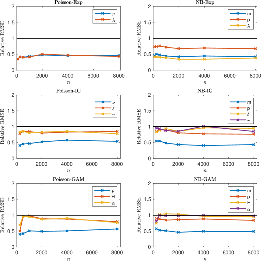
Figure 2: Root median square error (RMSE) of the MCL estimator (3.3) divided by the RMSE of the GMM estimator. The underlying IVT process $X_{t}$ is simulated on the grid $t=\Delta,2\Delta,\ldots,n\Delta$, with $\Delta=0.10$, see Table S1 for the values of the parameters used in the simulations. For the Poisson-Exp and NB-Exp models we set $K=1$ in Equations (S3.1) and (3.3); for the other models we set $K=10$.

6 Application to financial bid-ask spread data

In this section, we apply the IVT modelling framework to the bid-ask spread of equity prices. The bid-ask spread has been extensively studied in the market microstructure literature, see, e.g., Huang & Stoll (1997) and Bollen et al. (2004). An application similar to the one studied in this section was considered in Barndorff-Nielsen et al. (2014). To illustrate the use of the methods proposed in this paper, we study the time series of the bid-ask spread, measured in U.S. dollar cents, of the Agilent Technologies Inc. stock (ticker: A) on a single day, May $4$, $2020$. We cleaned the data and sampled the data in 5s intervals, leading to $n=3961$ observations, see Section S7 in the Supplementary Material for details.

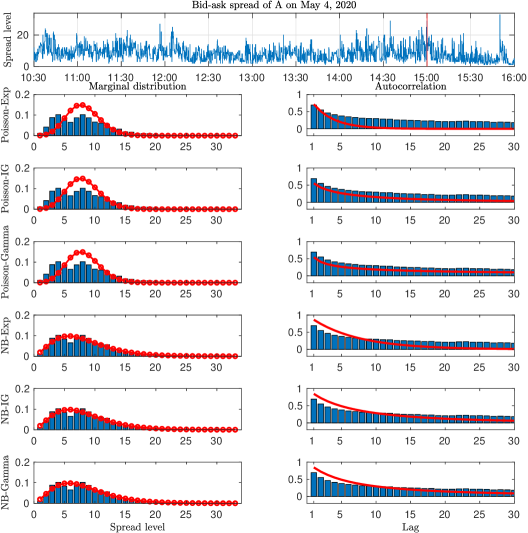
Figure 3: Analysis of the A spread level on May 4, 2020. Top: The data (spread level in cents) from $10$:$30$AM to $4$:$00$PM sampled every $5$ seconds. The vertical red line separates the initial in-sample period (left) from the out-of-sample period (right), used in the forecasting exercise in Section 6.1. The bottom six rows show the empirical autocorrelation (left; blue bars) and the empirical marginal distribution of the spread level (right; blue bars) together with the fits from the six IVT models (red lines). The parameters of the models have been estimated using the MCL estimator (3.3) with $K=10$, see Table 2.

Let $s_{t}$ be the bid-ask spread level at time $t$, the time series of which is displayed in the top panel of Figure 3. Since the minimum spread level in the data is one tick (one dollar cent), we work on this time series minus one, i.e on $x_{t}=s_{t}-1$. We can now apply our model selection method. We first inspect the empirical autocorrelation of the data (shown in the right panels of Figure 3) which shows evidence of a very persistent process; we, therefore, set $K$ to a moderately large value to accurately capture the dependence structure of the data. Here, we choose $K=10$ but the results are robust to other choices.

Table 1: Model selection results: bid-ask spread data

Model:	Poisson-Exponential	Poisson-IG	Poisson-Gamma	NB-Exponential	NB-IG	NB-Gamma
$CL$	$-244125.5$	$-242885.2$	$-242835.8$	$-216363.9$	$-216318.1$	${\bf-216313.5}$
$CLAIC$	$-244125.7$	$-242899.1$	$-242855.8$	$-216364.0$	$-216318.5$	${\bf-216313.9}$
$CLBIC$	$-244126.4$	$-242942.8$	$-242918.8$	$-216364.1$	$-216319.7$	${\bf-216315.1}$

Composite likelihood and information criteria values for fitting the A bid-ask spread data on May 4, 2020, shown in the top plot of Figure 3, calculated using six different models as given in the top row of the table using $K=10$. The maximum value for a given criteria (i.e. row-wise) is given in bold. The parameter estimates corresponding to the fits are given in Table 2.

Table 2: Estimation results: bid-ask spread data

DGP	$\nu$	$m$	$p$	$\lambda$	$\delta$	$\gamma$	$H$	$\alpha$
P-Exp	$28.9319$			$4.0399$
	$(0.6644)$			$(0.0904)$
P-IG	$294.9102$				$1.5293$	$0.0371$
	$(28.2715)$				$(0.0424)$	$(0.0040)$
P-Gamma	$83.8197$						$0.6123$	$0.0523$
	$(-)$						$(-)$	$(-)$
NB-Exp		$6.4273$	$0.6665$	$1.7835$
		$(0.9324)$	$(0.0215)$	$(0.1349)$
NB-IG		$7.7104$	$0.6675$		$1.7816$	$0.8292$
		$(1.0111)$	$(0.0238)$		$(0.4436)$	$(0.2094)$
NB-Gamma		$7.7336$	$0.6675$				$1.7020$	$0.7897$
		$(1.1316)$	$(0.0260)$				$(0.7365)$	$(0.3363)$

Parameter estimates (standard errors in parentheses) from the six different DGPs when applied to the bid-ask spread data of A on May 4, 2020 using the MCL estimator with $K=10$. The standard errors have been obtained using the simulation-based approach to estimating the asymptotic covariance matrix of the MCL estimator, see Section S4 in the Supplementary Material. Since our asymptotic theory does not cover the long memory case, no standard deviations are reported for the P-Gamma model. See Figure 3 for the resulting fits of the models to the empirical distribution and autocorrelation.

Using this setting, we calculated the maximized composite likelihood value, CL, and the two information criteria, $CLAIC$ and $CLBIC$, obtained for these data using the six models considered in Section 5. The results are shown in Table 1. The table shows that the NB-Gamma model is the preferred model on all three criteria, while the second-best model is the NB-IG model.

To further examine the fit of the various models, the bottom six rows of Figure 3 contain the empirical autocorrelation (left; blue bars) and the empirical marginal distribution of the spread level (right; blue bars). Each respective row also shows the fit of one of the six models considered in Table 1; the parameter estimates corresponding to the models are given in Table 2. The fit of the models shown in the bottom six panels of Figure 3 and the selection criteria of Table 1 indicate that the models based on the Negative Binomial distribution are preferred to the models based on the Poisson distribution. We conclude that, for this data series, the Poisson distribution is unable to accurately describe the marginal distribution of the spread level sampled every $5$ seconds. That the Gamma and IG trawl functions are preferred to the Exponential trawl function indicates that the Exponential autocorrelation function is not flexible enough to capture the correlation structure of the data. By both visual inspection of the autocorrelations in Figure 3 and the selection criteria of Table 1, we conclude that the NB-Gamma model is the preferred model for these data. As shown in Table 2, this model has $\hat{H}=1.70$ (s.e. $0.74$), implying that the model possesses a slowly decaying autocorrelation structure, albeit not the long memory property.

6.1 Forecasting the spread level

This section illustrates the use of IVT models for forecasting, as outlined in Section 4. The aim is to forecast the future spread level of the A stock on May $4$, i.e. the data studied above and plotted in the top panel of Figure 3. We set aside the first $n_{1}=3221$ observations as an “in-sample period” for initial estimation of the parameters of the models, see the vertical red line in the top panel of Figure 3 for the placement of this split. We then forecast the spread level from $5$ seconds until $100$ seconds into the future, using the approach presented in Section 4. That is, we forecast $x_{n_{1}+1},x_{n_{1}+2},\ldots,x_{n_{1}+20}$ given the current value $x_{n_{1}}$. After this, we update the in-sample data set with one additional observation so that this sample now contains $n_{2}=n_{1}+1=3222$ observations. Then we again forecast the next $20$ observations, $x_{n_{2}+1},x_{n_{2}+2},\ldots,x_{n_{2}+20}$, given $x_{n_{2}}$. We repeat this procedure until the end of the sample, which yields $n_{oos}=n-n_{1}-20=720$ out-of-sample forecasts for each forecast horizon. To ease the computational burden, we only re-estimate the model every $24$ periods (i.e. every $2$ minutes).

To evaluate the forecasts, we consider four different loss metrics. The first two, the mean absolute error (MAE) and the mean squared error (MSE), are often used in econometric forecasting studies of real-valued data (e.g. Elliott & Timmermann, 2016). For a forecast horizon $h=1,2,\ldots,20$, define the mean absolute forecast error,

$$MAE(h)=\frac{1}{n_{oos}}\sum_{i=n_{1}+h}^{n-(20-h)}|x_{i}-\hat{x}_{i|i-h}|,$$

where $\hat{x}_{i|i-h}$ is the $h$-step ahead forecast of $x_{i}$, constructed using the information available up to observation $i-h$. That is, $\hat{x}_{i|i-h}$ is the point forecast of $x_{i}$ coming from a particular IVT model, such as the conditional mean, median, or mode. In what follows, we set $\hat{x}_{i|i-h}$ equal to the estimated conditional mean, i.e. we set $\hat{x}_{i|i-h}=\sum_{k=0}^{M}\widehat{\mathbb{P}}(X_{i|i-h}=k)k$, where $M\geq 1$ is a large (cut-off) number and $\widehat{\mathbb{P}}$ is the estimated predictive density of the IVT model. Here, we set $M=60$ but the results are very robust to other choices. Define also the mean squared forecast error

$$MSE(h)=\frac{1}{n_{oos}}\sum_{i=n_{1}+h}^{n-(20-h)}(x_{i}-\hat{x}_{i|i-h})^{2}.$$

We consider two additional loss metrics, designed to directly evaluate the accuracy of the estimated predictive PMF $\widehat{\mathbb{P}}$, which is arguably more relevant to the problem at hand than MAE and MSE. The first is the logarithmic score (Elliott & Timmermann, 2016, p. 30),

$$logS(h)=\frac{1}{n_{oos}}\sum_{i=n_{1}+h}^{n-(20-h)}-\log\widehat{\mathbb{P}}(X_{i|i-h}=x_{i}),$$

where $x_{i}$ is the realized outcome. The second is the ranked probability score (RPS; Epstein, 1969),

$$RPS(h)=\frac{1}{n_{oos}}\sum_{i=n_{1}+h}^{n-(20-h)}\sum_{k=0}^{M}(\widehat{F}_{i|i-h}(k)-\mathbb{I}_{\{x_{i}\leq k\}})^{2},$$

where $\widehat{F}_{i|i-h}(k)=\sum_{j=0}^{k}\widehat{\mathbb{P}}(X_{i|i-h}=j)$ is the estimated cumulative distribution function of $X_{i}|x_{i-h}$ coming from a given model and $\mathbb{I}_{\{x_{i}\leq k\}}$ is the indicator function of the event $\{x_{i}\leq k\}$.

Figure 4 shows the four different forecast loss metrics for the preferred NB-Gamma IVT model as a ratio of the forecasting loss of a given benchmark model in the out-of-sample forecasting exercise described above. The numbers plotted in the figure are $Loss(h)_{NB-Gamma}/Loss(h)_{benchmark}$, where “$Loss$” denotes one of the four loss metrics given above and $h=1,2,\ldots,20$ denotes the forecasting horizon. Thus, numbers less than one favour the NB-Gamma model compared to the benchmark model and vice versa for numbers greater than one. Initially, we choose the Poisson-Exponential IVT process as the benchmark model (Figure 4, first column); as remarked above, this process is identical to the Poissonian INAR(1) model, which is often used for forecasting count-valued data (e.g. Freeland & McCabe, 2004; McCabe & Martin, 2005; Silva et al., 2009). It is evident from the figure that losses from the NB-Gamma model are smaller than those from the Poisson-Exponential model for practically all forecast horizons and loss metrics. In the case of the two most relevant loss functions for evaluating the predictive distribution, the logS and RPS, the reduction in losses are substantial for all forecast horizon, on the order of $20\%$.

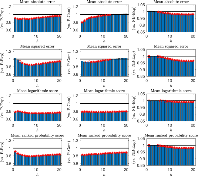
Figure 4: Forecasting the spread level of the A stock on May 4, 2020. Four different loss metrics (row-wise, as indicated above each plot) and twenty forecast horizons, $h=1,2,\ldots,20$. The numbers plotted are relative average losses of the NB-Gamma forecasting model, compared with the Poisson-Exponential model (first column), the Poisson-Gamma model (second column), and the NB-Exponential model (third column), over $n_{oos}=720$ out-of-sample forecasts. A circle above the bars indicates rejection null of equal forecasting performance between the two models, against the alternative that the NB-Gamma model provides superior forecasts, using the Diebold-Mariano (Diebold and Mariano, 1995) test at a $5\%$ level; an asterisk denotes rejection at a $1\%$ level.

To assess whether these loss differences are also statistically significant, we perform the Diebold-Mariano test of superior predictive ability (Diebold and Mariano, 1995). The null hypothesis of the statistical test is that the two models have equal predictive power, while the alternative hypothesis is that the NB-Gamma model provides superior forecasts compared to the benchmark model. In Figure 4, a circle (asterisk) denotes rejection of the Diebold-Mariano test at a $5\%$ ($1\%$) level. The test rejects the null hypothesis of equal predictive ability for almost all forecast horizons and loss metrics at a $1\%$ level.

To investigate whether the increased forecast performance of the NB-Gamma model comes from having a more flexible marginal distribution than the Poisson-Exponential benchmark model (Negative Binomial vs. Poisson marginals) or from having a more flexible correlation structure (polynomial decay vs. exponential decay) or both, we compare the forecasts from NB-Gamma model to those coming from a Poisson-Gamma model and from an NB-Exp model. These results are given in the second and third columns of Figure 4, respectively. From the second column, we see that the NB-Gamma model outperforms the Poisson-Gamma model considerably, especially for the shorter forecast horizons, indicating that it is important to use a model with Negative Binomial marginals when forecasting these data. From the third column of the figure, we see that for the shorter forecast horizons, the NB-Exp model performs on par with the NB-Gamma model, but for the longer forecast horizons, the NB-Gamma model is superior. Hence, when forecasting, it also appears to be important to specify a model with an accurate autocorrelation structure, especially for longer forecasting horizons.

7 Conclusion

This paper has developed likelihood-based methods for the estimation, inference, model selection, and forecasting of IVT processes. We proved the consistency and asymptotic normality of the MCL estimator and provided the details on how to conduct feasible inference and model selection. We also developed a pairwise approach to approximating the conditional predictive PMF of the IVT process, which can be used for forecasting integer-valued data. All these methods are implemented in a freely available software package written in the MATLAB programming language.

In a simulation exercise, we demonstrated the good properties of the MCL estimator compared to the often-used method-of-moments-based estimator. Indeed, the reduction in root median squared error of the MCL estimator was in many cases more than $50\%$ compared to the corresponding GMM estimator.

In an empirical application to financial bid-ask spread data, we illustrated the model selection procedure and found that the Negative Binomial-Gamma IVT model provided the best fit for the data. Using the forecast tools developed in the paper, we saw that this model outperformed the simpler Poisson-Exponential IVT model considerably, resulting in a reduction in forecast loss on the order of $20\%$ for most forecast horizons. We demonstrated that most of the superior forecasting performance came from accurate modelling of the marginal distribution of the data; however, we also found that it was beneficial to carefully model the autocorrelation structure, especially for longer forecasting horizons. These findings highlight the strengths of the IVT modelling framework, where the marginal distribution and autocorrelation structure can be modelled independently in a flexible fashion.

Appendix A Mathematical proofs

We first give an alternative representation of the Lévy basis $L$, underlying the IVT process X. From the construction of the IVT process in Section 2 in the main article, it is clear that the distribution of $L$ is representable as a compound Poisson distribution. That is, for a Borel set $B$, we can write

$$\mathbb{P}_{\theta}(L(B)=x) =\sum_{q=0}^{\infty}\mathbb{P}_{\theta}\left(\sum_{i=1}^{q}Y_{i}=x,\tilde{N}(B)=q\right)$$

$$=\sum_{q=0}^{\infty}\mathbb{P}_{\theta}\left(\sum_{i=1}^{q}Y_{i}=x\right)\mathbb{P}_{\theta}(\tilde{N}(B)=q),\quad x\in\mathbb{Z},$$ (A.1)

where $Y_{i}$ are iid integer-valued random variables with probability mass function $\tilde{\eta}(y):=\frac{\eta(y)}{\sum_{y=-\infty}^{\infty}\eta(y)}$, i.e. $\mathbb{P}_{\theta}(Y_{i}=y)=\tilde{\eta}(y)$, where $\eta$ is the Lévy measure given in the construction of the IVT process in Equation. Likewise, $\tilde{N}$ is a Poisson random measure, given by

$$\tilde{N}(dx,ds)=\int_{-\infty}^{\infty}N(dy,dx,ds),$$

with an underlying intensity $\tilde{\nu}:=\sum_{y=-\infty}^{\infty}\eta(y)$. The random variables $Y_{i}$ are independent of the random measure $\tilde{N}$. Intuitively, we have decomposed the event that the sum of the points in the set $B$ equals $x$ (i.e. $\{L(B)=x\}$) into the intersection of the two events that there are $q$ individual points in $B$ (i.e. $\{\tilde{N}(B)=q\}$) and the “sizes” of these $q$ points add up to $x$ (i.e. $\{\sum_{i=1}^{q}Y_{i}=x\}$). With this construction, we have

$$\mathbb{P}_{\theta}(\tilde{N}(B)=q)=\frac{(\tilde{\nu}Leb(B))^{q}}{q!}e^{-\tilde{\nu}Leb(B)},\quad q=0,1,2,\ldots.$$ (A.2)

We will use this alternative representation of $L$ in our proofs below.

Proof of Theorem 3.1.

Let $m>0$ and define $N_{m}=\tilde{N}(A_{m}\cap A)$ as the Poisson random variable, which counts the number of ‘events’ in the set $A_{m}\cap A_{0}$. From (A.2), we know that there exists a constant $\tilde{\nu}>0$ such that

$$\mathbb{P}(N_{m}=0)=e^{-\tilde{\nu}Leb(A_{m}\cap A_{0})}$$

and, therefore,

$$\mathbb{P}(N_{m}\neq 0)=1-\mathbb{P}(N_{m}=0)=1-e^{-\tilde{\nu}Leb(A_{m}\cap A_{0})}=\tilde{\nu}Leb(A_{m}\cap A_{0})+o(Leb(A_{m}\cap A_{0})),$$ (A.3)

as $m\rightarrow\infty$.

Let $G\in\mathcal{F}_{-\infty}^{0}$ and $H\in\mathcal{F}_{m}^{\infty}$ be such that $\mathbb{P}(G),\mathbb{P}(H)>0$, and write, using the law of total probability,

$$|\mathbb{P}(H\cap G)-\mathbb{P}(H)\mathbb{P}(G)| =|\mathbb{P}(H|G)-\mathbb{P}(H)|\cdot\mathbb{P}(G)$$

$$=|\mathbb{P}(H|G,N_{m}=0)\mathbb{P}(N_{m}=0|G)+\mathbb{P}(H|G,N_{m}\neq 0)\mathbb{P}(N_{m}\neq 0|G)$$

$$-\mathbb{P}(H|N_{m}=0)\mathbb{P}(N_{m}=0)-\mathbb{P}(H|N_{m}\neq 0)\mathbb{P}(N_{m}\neq 0)|\cdot\mathbb{P}(G)$$

$$\leq(D_{1,m}+D_{2,m})\cdot\mathbb{P}(G),$$

where

$$D_{1,m} :=|\mathbb{P}(H|G,N_{m}=0)\mathbb{P}(N_{m}=0|G)-\mathbb{P}(H|N_{m}=0)\mathbb{P}(N_{m}=0)|,$$

$$D_{2,m} :=|\mathbb{P}(H|G,N_{m}\neq 0)\mathbb{P}(N_{m}\neq 0|G)-\mathbb{P}(H|N_{m}\neq 0)\mathbb{P}(N_{m}\neq 0)|.$$

We seek to bound these expressions. For $D_{1,m}$, we use the fact that on the event $\{N_{m}=0\}$ the two events $G$ and $H$ are independent. For both $D_{1,m}$ and $D_{2,m}$, we will use that the probability of the complementary event $\{N_{m}\neq 0\}$ is “small enough”, cf. Equation (A.3). For the first of the terms, we get, using conditional independence of $H$ and $G$ and (A.3),

$$D_{1,m} =\mathbb{P}(H|N_{m}=0)\cdot|\mathbb{P}(N_{m}=0|G)-\mathbb{P}(N_{m}=0)|$$

$$\leq|\mathbb{P}(N_{m}=0|G)-\mathbb{P}(N_{m}=0)|$$

$$\leq|1-\mathbb{P}(N_{m}=0|G)|+|1-\mathbb{P}(N_{m}=0)|$$

$$=|1-\mathbb{P}(N_{m}=0|G)|+\tilde{\nu}Leb(A_{m}\cap A_{0})+o(Leb(A_{m}\cap A_{0})),$$

and, using the Bayes formula and then the law of total probability,

$$|1-\mathbb{P}(N_{m}=0|G)| =|1-\mathbb{P}(G|N_{m}=0)\mathbb{P}(N_{m}=0)\mathbb{P}(G)^{-1}|$$

$$=\mathbb{P}(G)^{-1}|\mathbb{P}(G)-\mathbb{P}(G|N_{m}=0)\mathbb{P}(N_{m}=0)|$$

$$=\mathbb{P}(G)^{-1}|\mathbb{P}(G|N_{m}=0)\mathbb{P}(N_{m}=0)+\mathbb{P}(G|N_{m}\neq 0)\mathbb{P}(N_{m}\neq 0)$$

$$-\mathbb{P}(G|N_{m}=0)\mathbb{P}(N_{m}=0)|$$

$$=\mathbb{P}(G)^{-1}|\mathbb{P}(G|N_{m}\neq 0)\mathbb{P}(N_{m}\neq 0)|$$

$$\leq\mathbb{P}(G)^{-1}\mathbb{P}(N_{m}\neq 0)$$

$$=\mathbb{P}(G)^{-1}(\tilde{\nu}Leb(A_{m}\cap A_{0})+o(Leb(A_{m}\cap A_{0}))).$$

We conclude that

$$D_{1,m}\cdot\mathbb{P}(G)\leq 2\tilde{\nu}Leb(A_{m}\cap A_{0})+o(Leb(A_{m}\cap A_{0})).$$

For the second term above, we get

$$D_{2,m} =|\mathbb{P}(H|G,N_{m}\neq 0)\mathbb{P}(N_{m}\neq 0|G)-\mathbb{P}(H|N_{m}\neq 0)\mathbb{P}(N_{m}\neq 0)|$$

$$=|\mathbb{P}(H|G,N_{m}\neq 0)\mathbb{P}(N_{m}\neq 0|G)-\mathbb{P}(H|G,N_{m}\neq 0)\mathbb{P}(N_{m}\neq 0)$$

$$+\mathbb{P}(H|G,N_{m}\neq 0)\mathbb{P}(N_{m}\neq 0)-\mathbb{P}(H|N_{m}\neq 0)\mathbb{P}(N_{m}\neq 0)|$$

$$\leq E_{1,m}+E_{2,m},$$

where

$$E_{1,m} :=|\mathbb{P}(H|G,N_{m}\neq 0)\mathbb{P}(N_{m}\neq 0|G)-\mathbb{P}(H|G,N_{m}\neq 0)\mathbb{P}(N_{m}\neq 0)|,$$

$$E_{2,m} :=|\mathbb{P}(H|G,N_{m}\neq 0)\mathbb{P}(N_{m}\neq 0)-\mathbb{P}(H|N_{m}\neq 0)\mathbb{P}(N_{m}\neq 0)|.$$

Now, by (A.3),

$$E_{2,m} =\mathbb{P}(N_{m}\neq 0)|\mathbb{P}(H|G,N_{m}\neq 0)-\mathbb{P}(H|N_{m}\neq 0)|$$

$$\leq\mathbb{P}(N_{m}\neq 0)$$

$$=\tilde{\nu}Leb(A_{m}\cap A_{0})+o(Leb(A_{m}\cap A_{0})).$$

Also,

$$E_{1,m} =|\mathbb{P}(H|G,N_{m}\neq 0)\mathbb{P}(N_{m}\neq 0|G)-\mathbb{P}(H|G,N_{m}\neq 0)\mathbb{P}(N_{m}\neq 0)|$$

$$=\mathbb{P}(H|G,N_{m}\neq 0)\cdot|\mathbb{P}(N_{m}\neq 0|G)-\mathbb{P}(N_{m}\neq 0)|$$

$$\leq|\mathbb{P}(N_{m}\neq 0|G)-\mathbb{P}(N_{m}\neq 0)|$$

$$\leq\mathbb{P}(N_{m}\neq 0|G)+\mathbb{P}(N_{m}\neq 0).$$

Using Bayes formula, we can write

$$\mathbb{P}(N_{m}\neq 0|G) =\mathbb{P}(G|N_{m}\neq 0)\mathbb{P}(N_{m}\neq 0)\mathbb{P}(G)^{-1}$$

$$\leq\mathbb{P}(N_{m}\neq 0)\mathbb{P}(G)^{-1}$$

so that, from (A.3),

$$E_{1,m}\leq(1+\mathbb{P}(G)^{-1})(\tilde{\nu}Leb(A_{m}\cap A_{0})+o(Leb(A_{m}\cap A_{0}))).$$

We conclude that

$$D_{2,m}\cdot\mathbb{P}(G)\leq 3\tilde{\nu}Leb(A_{m}\cap A_{0})+o(Leb(A_{m}\cap A_{0})).$$

Taking it all together, we have that

$$|\mathbb{P}(H\cap G)-\mathbb{P}(H)\mathbb{P}(G)| \leq(D_{1,m}+D_{2,m})\cdot\mathbb{P}(G)$$

$$\leq 5\tilde{\nu}Leb(A_{m}\cap A_{0})+o(Leb(A_{m}\cap A_{0})),$$

implying, since $G$ and $H$ were arbitrary, that (taking supremums)

$$\alpha_{m}\leq 5\tilde{\nu}Leb(A_{m}\cap A_{0})+o(Leb(A_{m}\cap A_{0})),$$

which implies that $\alpha_{m}\leq O(Leb(A_{m}\cap A_{0}))$.

To finish the proof, we show that we also have $\alpha_{m}\geq O(Leb(A_{m}\cap A_{0}))$. Letting $x_{1},x_{2}\in\mathbb{Z}$ and defining the events $\tilde{H}:=\{X_{0}=x_{1}\}$ and $\tilde{G}:=\{X_{m}=x_{2}\}$, the results and the arguments in the proof of Lemma A.1 imply that

$$|\mathbb{P}(\tilde{H}\cap\tilde{G})-\mathbb{P}(\tilde{H})\mathbb{P}(\tilde{G})|=O(Leb(A_{m}\cap A_{0})),\qquad m\rightarrow\infty.$$

Since, clearly, $\tilde{H}\in\mathcal{F}_{-\infty}^{0}$ and $\tilde{G}\in\mathcal{F}_{m}^{\infty}$, we conclude that $\alpha_{m}=\sup_{H\in\mathcal{F}_{-\infty}^{0},G\in\mathcal{F}_{m}^{\infty}}|\mathbb{P}(H\cap G)-\mathbb{P}(H)\mathbb{P}(G)|\geq|\mathbb{P}(\tilde{H}\cap\tilde{G})-\mathbb{P}(\tilde{H})\mathbb{P}(\tilde{G})|=O(Leb(A_{m}\cap A_{0}))$.

∎

Proof of Proposition 3.1.

When $\nu(y)=0$ for $y<0$ we have $P_{\theta}(L(A_{(i+k)\Delta}\cap A_{i\Delta})=c)=0$ for $c<0$. Further, since the maximal amount of events in $L(A_{(i+k)\Delta}\cap A_{i\Delta})$ is bounded by the number of events in $x_{t+k}$ and $x_{t}$ (no negative values in the trawl sets), we also have $P_{\theta}(L(A_{(i+k)\Delta}\cap A_{i\Delta})=c)=0$ for $c>\min\{x_{t+k},x_{t}\}$. This, together with the discussion of the decomposition of trawl sets in Section 3.1.1 (cf. Figure S1 in the Supplementary Material), and the law of total probability implies that

$$f(x_{i+k}, x_{i};\theta):=\mathbb{P}_{\theta}\left(X_{(i+k)\Delta}=x_{i+k},X_{i\Delta}=x_{i}\right)$$

$$= \sum_{c=-\infty}^{\infty}\mathbb{P}_{\theta}\left(X_{(i+k)\Delta}=x_{i+k},X_{i\Delta}=x_{i}|L(A_{(i+k)\Delta}\cap A_{i\Delta})=c\right)\cdot\mathbb{P}_{\theta}\left(L(A_{(i+k)\Delta}\cap A_{i\Delta})=c\right)$$

$$= \sum_{c=0}^{\max\{x_{i},x_{i+k}\}}\mathbb{P}_{\theta}\left(L(A_{(i+k)\Delta}\setminus A_{i\Delta})=x_{i+k}-c\right)\mathbb{P}_{\theta}\left(L(A_{i\Delta}\setminus A_{(i+k)\Delta})=x_{i}-c\right)$$

$$\cdot\mathbb{P}_{\theta}\left(L(A_{(i+k)\Delta}\cap A_{i\Delta})=c\right),$$

as we wanted to show. ∎

Proof of Theorem 3.2.

Due to the stationarity and ergodicity of the IVT processes considered in this paper, the normalized log-composite likelihood function will converge in probability to its population counterpart, i.e.

$$Q_{n}(\theta):=\frac{1}{n}l_{CL}(\theta;X)=\frac{1}{n}\sum_{k=1}^{K}\sum_{i=1}^{n-k}\log f(X_{(i+k)\Delta},X_{i\Delta};\theta)\stackrel{{\scriptstyle\mathbb{P}}}{{\rightarrow}}\mathbb{E}\left[\sum_{k=1}^{K}\log f(X_{k\Delta},X_{0};\theta)\right]=:Q(\theta),$$

as $n\rightarrow\infty$. By the identifiability condition (3.5), and the fact that the pairwise likelihoods are indeed proper (bivariate) likelihoods, the information inequality implies that $Q(\theta)$ is uniquely maximized at $\theta=\theta_{0}$ (Lemma 2.2 in Newey & McFadden 1994, p. 2124). The result now follows from Theorem 4.1 and Theorem 4.3 in Wooldridge (1994). ∎

Proof of Theorem 3.3.

Let

$$s_{n}(\theta):=\frac{\partial}{\partial\theta}l_{CL}(\theta;X)=\sum_{k=1}^{K}\sum_{i=1}^{n-k}\frac{\partial}{\partial\theta}\log f(X_{(i+k)\Delta},X_{i\Delta};\theta)$$

denote the score function and consider the estimating equation related to the MCL estimator $\hat{\theta}=\hat{\theta}^{CL}$, namely $s_{n}(\hat{\theta})=0$. Using this equation, we Taylor expand $s_{n}(\hat{\theta})$ around the true parameter vector $\theta_{0}$ to get

$$s_{n}(\theta_{0})+\frac{\partial}{\partial\theta^{\prime}}s_{n}(\bar{\theta})(\hat{\theta}-\theta_{0})=0,$$

where $\bar{\theta}$ lies on the line segment between $\theta_{0}$ and $\hat{\theta}$ and $\frac{\partial}{\partial\theta^{\prime}}s_{n}(\bar{\theta})$ is shorthand for $\frac{\partial}{\partial\theta^{\prime}}s_{n}(\theta)|_{\theta=\bar{\theta}}$. Rearranging this equation and multiplying through by $\sqrt{n}$, we get

$$\sqrt{n}(\hat{\theta}-\theta_{0})=-\left(\frac{1}{n}\frac{\partial}{\partial\theta^{\prime}}s_{n}(\bar{\theta})\right)^{-1}n^{-1/2}s_{n}(\theta_{0}).$$

Stationarity and ergodicity, along with consistency of $\hat{\theta}$ due to Theorem 3.2, implies that $-\frac{1}{n}\frac{\partial}{\partial\theta^{\prime}}s_{n}(\bar{\theta})^{\prime}\stackrel{{\scriptstyle\mathbb{P}}}{{\rightarrow}}H(\theta_{0})$ as $n\rightarrow\infty$. To prove the result, we thus need to show that $n^{-1/2}s_{n}(\theta_{0})\stackrel{{\scriptstyle(d)}}{{\rightarrow}}N(0,V(\theta_{0}))$ as $n\rightarrow\infty$. By the mixing properties of the IVT process $X$, given in Theorem 3.1, it is enough to show that $\mathbb{E}[s_{n}(\theta_{0})]=0$ and $Var\left(n^{-1/2}s_{n}(\theta_{0})\right)\rightarrow V(\theta_{0})$ as $n\rightarrow\infty$ (e.g. Davidson 1994, Corollary 24.7, p. 387).

To show this, we consider, for simplicity, the case where $\theta$ is a scalar. The vector case is similar, but with slightly more involved notation. First note that, clearly,

$$\mathbb{E}\left[s_{n}(\theta_{0})\right]=\mathbb{E}\left[\frac{\partial}{\partial\theta}l_{CL}(\theta;X)|_{\theta=\theta_{0}}\right]=0.$$

Also

$$Var\left(s_{n}(\theta_{0})\right) =Var\left(\frac{\partial}{\partial\theta}l_{CL}(\theta;X)|_{\theta=\theta_{0}}\right)$$

$$=Var\left(\sum_{k=1}^{K}\sum_{i=1}^{n-k}\frac{\partial}{\partial\theta}\log\left.f(X_{i\Delta},X_{(i+k)\Delta};\theta)\right|_{\theta=\theta_{0}}\right)$$

$$=\sum_{k=1}^{K}\sum_{i=1}^{n-k}Var\left(\frac{\partial}{\partial\theta}\log\left.f(X_{i\Delta},X_{(i+k)\Delta};\theta)\right|_{\theta=\theta_{0}}\right)$$

$$+\sum_{k=1}^{K}\sum_{k^{\prime}=1}^{K}\sum_{i\neq j}Cov\left(\frac{\partial}{\partial\theta}\log\left.f(X_{i\Delta},X_{(i+k)\Delta};\theta)\right|_{\theta=\theta_{0}},\frac{\partial}{\partial\theta}\log\left.f(X_{j\Delta},X_{(j+k^{\prime})\Delta};\theta)\right|_{\theta=\theta_{0}}\right).$$

Due to stationarity, the first sum is $O(n)$ as $n\rightarrow\infty$. To prove the proposition, we, therefore, investigate the second sum. With slight abuse of notation, let $\frac{\partial}{\partial\theta}\log\left.f(X_{i\Delta},X_{(i+k)\Delta};\theta)\right|_{\theta=\theta_{0}}$ be denoted by $\frac{\partial}{\partial\theta}\log f(X_{i\Delta},X_{(i+k)\Delta};\theta_{0})$. For $l,k,k^{\prime}\geq 1$, define also the joint probability mass functions

$$f_{l}(x_{1},x_{2},x_{3},x_{4};k,k^{\prime},\theta):=\mathbb{P}_{\theta}\left(X_{0}=x_{1},X_{k\Delta}=x_{2},X_{l\Delta}=x_{3},X_{(l+k^{\prime})\Delta}=x_{4}\right),\quad x_{1},x_{2},x_{3},x_{4}\in\mathbb{Z}.$$

and

$$f_{k}(x_{1},x_{2}):=\mathbb{P}_{\theta}\left(X_{0}=x_{1},X_{k\Delta}=x_{2}\right),\quad x_{1},x_{2}\in\mathbb{Z}.$$

Now, using that

$$\mathbb{E}\left[\frac{\partial}{\partial\theta}\log f(X_{i\Delta},X_{(i+k)\Delta};\theta_{0})\right]=0,$$

we have, for all $i,j,k,k^{\prime}$,

$$Cov\left(\frac{\partial}{\partial\theta}\log f(X_{i\Delta},X_{(i+k)\Delta};\theta_{0}),\frac{\partial}{\partial\theta}\log f(X_{j\Delta},X_{(j+k^{\prime})\Delta};\theta_{0})\right)$$

$$=\mathbb{E}\left[\frac{\partial}{\partial\theta}\log f(X_{i\Delta},X_{(i+k)\Delta};\theta_{0})\frac{\partial}{\partial\theta}\log f(X_{j\Delta},X_{(j+k^{\prime})\Delta};\theta_{0})\right]$$

$$=\sum_{x_{1}=-\infty}^{\infty}\sum_{x_{2}=-\infty}^{\infty}\sum_{x_{3}=-\infty}^{\infty}\sum_{x_{4}=-\infty}^{\infty}\frac{\partial}{\partial\theta}f_{k}(x_{1},x_{2};\theta_{0})\frac{\partial}{\partial\theta}f_{k^{\prime}}(x_{3},x_{4};\theta_{0})\frac{f_{|i-j|}(x_{1},x_{2},x_{3},x_{4};k,k^{\prime},\theta_{0})}{f_{k}(x_{1},x_{2};\theta_{0})f_{k^{\prime}}(x_{3},x_{4};\theta_{0})}$$

$$=\sum_{x_{1}=-\infty}^{\infty}\sum_{x_{2}=-\infty}^{\infty}\sum_{x_{3}=-\infty}^{\infty}\sum_{x_{4}=-\infty}^{\infty}\frac{\partial}{\partial\theta}f_{k}(x_{1},x_{2};\theta_{0})\frac{\partial}{\partial\theta}f_{k^{\prime}}(x_{3},x_{4};\theta_{0})\left(\frac{f_{|i-j|}(x_{1},x_{2},x_{3},x_{4};k,k^{\prime},\theta_{0})}{f_{k}(x_{1},x_{2};\theta_{0})f_{k^{\prime}}(x_{3},x_{4};\theta_{0})}-1\right),$$

where the last equality follows because e.g.,

$$\sum_{x_{1}=-\infty}^{\infty}\sum_{x_{2}=-\infty}^{\infty}\frac{\partial}{\partial\theta}f_{k}(x_{1},x_{2};\theta_{0})=\frac{\partial}{\partial\theta}\sum_{x_{1}=-\infty}^{\infty}\sum_{x_{2}=-\infty}^{\infty}f_{k}(x_{1},x_{2};\theta_{0})=\frac{\partial}{\partial\theta}1=0.$$

Now, Lemma A.1 below shows that

$$\left(\frac{f_{n}(x_{1},x_{2},x_{3},x_{4};k,k^{\prime},\theta_{0})}{f_{k}(x_{1},x_{2};\theta_{0})f_{k^{\prime}}(x_{3},x_{4};\theta_{0})}-1\right)=O(Leb(A_{n\Delta}\cap A_{0})),\quad n\rightarrow\infty,$$

from which we conclude, using Equation (2.5), i.e. $Leb(A_{n\Delta}\cap A_{0})=\rho(n\Delta)Leb(A)$, and the condition on $\rho$ imposed in the theorem, that the second sum in the expression for $Var\left(s_{n}(\theta_{0})\right)$ is $O(n)$ as well. Indeed, taking it all together, we have that, as $n\rightarrow\infty$,

$$n^{-1}Var\left(s_{n}(\theta_{0})\right) \rightarrow\sum_{k=1}^{K}Var\left(\frac{\partial}{\partial\theta}\log\left.f(X_{0},X_{k\Delta};\theta)\right|_{\theta=\theta_{0}}\right)$$

$$+2\sum_{k=1}^{K}\sum_{k^{\prime}=1}^{K}\sum_{i=1}^{\infty}Cov\left(\frac{\partial}{\partial\theta}\log\left.f(X_{0},X_{k\Delta};\theta)\right|_{\theta=\theta_{0}},\frac{\partial}{\partial\theta}\log\left.f(X_{i\Delta},X_{(i+k^{\prime})\Delta};\theta)\right|_{\theta=\theta_{0}}\right)$$

$$=:V(\theta_{0}),$$

where the series converges. This finalizes the proof.

∎

Lemma A.1.

Fix $k,k^{\prime}\geq 1$, let $X$ be an IVT process, let $f_{k}(\cdot,\cdot;\theta)$ be the joint PMF of $(X_{0},X_{k\Delta})$, and let $f_{n}(\cdot,\cdot,\cdot,\cdot;k,k^{\prime},\theta)$ be the joint PMF of $(X_{0},X_{k\Delta},X_{n\Delta},X_{(n+k^{\prime})\Delta})$. That is

$$f_{k}(x_{1},x_{2};\theta):=\mathbb{P}_{\theta}\left(X_{0}=x_{1},X_{k\Delta}=x_{2}\right),\quad x_{1},x_{2}\in\mathbb{Z},$$

and

$$f_{n}(x_{1},x_{2},x_{3},x_{4};k,k^{\prime},\theta):=\mathbb{P}_{\theta}\left(X_{0}=x_{1},X_{k\Delta}=x_{2},X_{n\Delta}=x_{3},X_{(n+k^{\prime})\Delta}=x_{4}\right),\quad x_{1},x_{2},x_{3},x_{4}\in\mathbb{Z}.$$

Define the function

$$G_{n}(x_{1},x_{2},x_{3},x_{4};k,k^{\prime},\theta):=\left(\frac{f_{n}(x_{1},x_{2},x_{3},x_{4};k,k^{\prime},\theta)}{f_{k}(x_{1},x_{2};\theta)f_{k^{\prime}}(x_{3},x_{4};\theta)}-1\right).$$

The following holds:

$$\frac{1}{Leb(A_{k\Delta}\cap A_{n\Delta})}G_{n}(x_{1},x_{2},x_{3},x_{4};k,k^{\prime},\theta)\rightarrow G(x_{1},x_{2},x_{3},x_{4};k,k^{\prime},\theta),\quad n\rightarrow\infty,$$

where $G$ is a function, given in Equation (A.7) below, that depends on the Lévy basis and trawl function of $X$. (In Remark A.1 below, we give the function $G$ in the special case where the Lévy basis is Poissonian and the trawl function is the Gamma trawl.)

Proof of Lemma A.1.

Letting $f_{n}(x_{1},x_{2}|x_{3},x_{4};k,k^{\prime},\theta):=\mathbb{P}_{\theta}\left(X_{0}=x_{1},X_{k\Delta}=x_{2}|X_{n\Delta}=x_{3},X_{(n+k^{\prime})\Delta}=x_{4}\right)$, we can write

$$G_{n}(x_{1},x_{2},x_{3},x_{4};k,k^{\prime},\theta) =\frac{f_{n}(x_{1},x_{2},x_{3},x_{4};\theta)-f_{k}(x_{1},x_{2};\theta)f_{k^{\prime}}(x_{3},x_{4};\theta)}{f_{k}(x_{1},x_{2};\theta)f_{k^{\prime}}(x_{3},x_{4};\theta)}$$

$$=\frac{f_{n}(x_{1},x_{2}|x_{3},x_{4};k,k^{\prime},\theta)f_{k^{\prime}}(x_{3},x_{4};\theta)-f_{k}(x_{1},x_{2};\theta)f_{k^{\prime}}(x_{3},x_{4};\theta)}{f_{k}(x_{1},x_{2};\theta)f_{k^{\prime}}(x_{3},x_{4};\theta)}$$

$$=(f_{n}(x_{1},x_{2}|x_{3},x_{4};k,k^{\prime},\theta)-f_{k}(x_{1},x_{2};\theta))f_{k}(x_{1},x_{2};\theta)^{-1}.$$

To prove the lemma, we, therefore, study the asymptotic behaviour of $f_{n}(x_{1},x_{2}|x_{3},x_{4};k,k^{\prime},\theta)-f_{k}(x_{1},x_{2};\theta)$ as $n\rightarrow\infty$.

Recall first the decomposition of the trawl sets into three disjoint sets which led to Proposition 3.1, see Figure S1. In a similar manner, we can decompose the four trawl sets associated to $X_{0}=L(A_{0})$, $X_{k\Delta}=L(A_{k\Delta})$, $X_{n\Delta}=L(A_{n\Delta})$, and $X_{(n+k^{\prime})\Delta}=L(A_{(n+k^{\prime})\Delta})$, into $10$ disjoint sets as illustrated in Figure 5 below. For ease of notation, we ignore the dependence on $n$, $k$, and $k^{\prime}$ for a moment and write

$$A_{0} =C_{3}\cup C_{4}\cup C_{6}\cup C_{7},\quad A_{k\Delta}=C_{1}\cup C_{2}\cup C_{3}\cup C_{4}\cup C_{5}\cup C_{6},$$

$$A_{n\Delta} =C_{1}\cup C_{2}\cup C_{3}\cup C_{4}\cup D_{2}\cup D_{3},\quad A_{(n+k^{\prime})\Delta}=C_{1}\cup C_{3}\cup D_{1}\cup D_{2},$$

where the sets $C_{1},C_{2},\ldots,C_{7},D_{1},D_{2},D_{3}$ are disjoint. We will use below that $\lim_{n\rightarrow\infty}Leb(C_{j})=0$ for $j=1,2,3,4$, $\lim_{n\rightarrow\infty}Leb(C_{5})=Leb(A_{k\Delta}\setminus A_{0})$, $\lim_{n\rightarrow\infty}Leb(C_{6})=Leb(A_{0}\cap A_{k\Delta})$, $\lim_{n\rightarrow\infty}Leb(C_{7})=Leb(A_{0}\setminus A_{k\Delta})$, $\lim_{n\rightarrow\infty}Leb(D_{1})=Leb(A_{k^{\prime}\Delta}\setminus A_{0})$, $\lim_{n\rightarrow\infty}Leb(D_{2})=Leb(A_{0}\cap A_{k^{\prime}\Delta})$, and $\lim_{n\rightarrow\infty}Leb(D_{3})=Leb(A_{0}\setminus A_{k^{\prime}\Delta})$, cf. Figure 5.

Using this decomposition and the law of total probability, we may write

$$f(x_{1},x_{2};\theta) =\sum_{c_{1},c_{2},c_{3},c_{4}=-\infty}^{\infty}\mathbb{P}_{\theta}\left(L(C_{6})+L(C_{7})=x_{1}-c_{3}-c_{4},L(C_{5})+L(C_{6})=x_{2}-c_{1}-c_{2}-c_{3}-c_{4}\right)$$

$$\cdot\prod_{j=1}^{4}\mathbb{P}_{\theta}\left(L(C_{j})=c_{j}\right)$$

and

$$f(x_{1},x_{2}|x_{3},x_{4};\theta)$$

$$=\sum_{c_{1},c_{2},c_{3},c_{4}=-\infty}^{\infty}\mathbb{P}_{\theta}\left(L(C_{6})+L(C_{7})=x_{1}-c_{3}-c_{4},L(C_{5})+L(C_{6})=x_{2}-c_{1}-c_{2}-c_{3}-c_{4}\right)$$

$$\cdot\mathbb{P}_{\theta}\left(L(C_{1})=c_{1},L(C_{2})=c_{2},L(C_{3})=c_{3},L(C_{4})=c_{4}|X_{n\Delta}=x_{3},X_{(n+k^{\prime})\Delta}=x_{4}\right).$$

Taking these together, we get

$$f_{n}(x_{1},x_{2}|x_{3},x_{4};\theta)-f(x_{1},x_{2};\theta)$$

$$=\sum_{c_{1},c_{2},c_{3},c_{4}=-\infty}^{\infty}\mathbb{P}_{\theta}\left(L(C_{6})+L(C_{7})=x_{1}-c_{3}-c_{4},L(C_{5})+L(C_{6})=x_{2}-c_{1}-c_{2}-c_{3}-c_{4}\right)$$

$$\cdot\left(\mathbb{P}_{\theta}\left(L(C_{1})=c_{1},L(C_{2})=c_{2},L(C_{3})=c_{3},L(C_{4})=c_{4}|X_{n\Delta}=x_{3},X_{(n+k^{\prime})\Delta}=x_{4}\right)-\prod_{j=1}^{4}\mathbb{P}_{\theta}\left(L(C_{j})=c_{j}\right)\right).$$

Note that, for the first term in the parenthesis, the following holds

$$\mathbb{P}_{\theta}\left(L(C_{1})=c_{1},L(C_{2})=c_{2},L(C_{3})=c_{3},L(C_{4})=c_{4}|X_{n\Delta}=x_{3},X_{(n+k^{\prime})\Delta}=x_{4}\right)$$

$$=f(x_{3},x_{4};\theta)^{-1}\mathbb{P}_{\theta}\left(L(C_{1})=c_{1},L(C_{2})=c_{2},L(C_{3})=c_{3},L(C_{4})=c_{4},X_{n\Delta}=x_{3},X_{(n+k^{\prime})\Delta}=x_{4}\right)$$

$$=f(x_{3},x_{4};\theta)^{-1}\mathbb{P}_{\theta}\left(L(D_{2})+L(D_{3})=x_{3}-c_{1}-c_{2}-c_{3}-c_{4},L(D_{1})+L(D_{2})=x_{4}-c_{1}-c_{3}\right)$$

$$\cdot\prod_{j=1}^{4}\mathbb{P}_{\theta}\left(L(C_{j})=c_{j}\right),$$

which allows us to write

$$f_{n}(x_{1},x_{2}|x_{3},x_{4};\theta)-f(x_{1},x_{2};\theta)$$

$$=\sum_{c_{1},c_{2},c_{3},c_{4}=-\infty}^{\infty}\mathbb{P}_{\theta}\left(L(C_{6})+L(C_{7})=x_{1}-c_{3}-c_{4},L(C_{5})+L(C_{6})=x_{2}-c_{1}-c_{2}-c_{3}-c_{4}\right)$$

$$\cdot\prod_{j=1}^{4}\mathbb{P}_{\theta}\left(L(C_{j})=c_{j}\right)f(x_{3},x_{4};\theta)^{-1}$$

$$\cdot\left(\mathbb{P}_{\theta}\left(L(D_{2})+L(D_{3})=x_{3}-c_{1}-c_{2}-c_{3}-c_{4},L(D_{1})+L(D_{2})=x_{4}-c_{1}-c_{3}\right)-f(x_{3},x_{4})\right).$$

Define the set $\mathcal{C}_{0}:=\{(c_{1},c_{2},c_{3},c_{4})\in\mathbb{Z}^{4}:c_{i}\neq 0\textnormal{ for at least one }i=1,2,3,4\}$. The above calculations imply that

$$f_{n}(x_{1},x_{2}|x_{3},x_{4};\theta)-f(x_{1},x_{2};\theta)=f(x_{3},x_{4})^{-1}\left(F_{n}^{(1)}+F_{n}^{(2)}\right),$$ (A.4)

where

$$F_{n}^{(1)} :=\mathbb{P}_{\theta}\left(L(C_{6})+L(C_{7})=x_{1},L(C_{5})+L(C_{6})=x_{2}\right)\prod_{j=1}^{4}\mathbb{P}_{\theta}\left(L(C_{j})=0\right)$$

$$\cdot\left(\mathbb{P}_{\theta}\left(L(D_{2})+L(D_{3})=x_{3},L(D_{1})+L(D_{2})=x_{4}\right)-f(x_{3},x_{4};\theta)\right)$$

and

$$F_{n}^{(2)} :=\sum_{(c_{1},c_{2},c_{3},c_{4})\in\mathcal{C}_{0}}\mathbb{P}_{\theta}\left(L(C_{6})+L(C_{7})=x_{1}-c_{3}-c_{4},L(C_{5})+L(C_{6})=x_{2}-c_{1}-c_{2}-c_{3}-c_{4}\right)$$

$$\cdot\prod_{j=1}^{4}\mathbb{P}_{\theta}\left(L(C_{j})=c_{j}\right)$$

$$\cdot\left(\mathbb{P}_{\theta}\left(L(D_{2})+L(D_{3})=x_{3}-c_{1}-c_{2}-c_{3}-c_{4},L(D_{1})+L(D_{2})=x_{4}-c_{1}-c_{3}\right)-f(x_{3},x_{4};\theta)\right).$$

We can think of $F_{n}^{(1)}$ as the part of $(f_{n}(x_{1},x_{2}|x_{3},x_{4};\theta)-f(x_{1},x_{2};\theta))f(x_{3},x_{4})$ where $c_{1}=c_{2}=c_{3}=c_{4}=0$, while $F_{n}^{(2)}$ is the remainder.

We study first the behavior of $F_{n}^{(1)}$ as $n\rightarrow\infty$. Considering the first two factors of this term, the continuity of the probability measure $\mathbb{P}_{\theta}(\cdot)$ implies that

$$\lim_{n\rightarrow\infty}\mathbb{P}_{\theta}\left(L(C_{6})+L(C_{7})=x_{1},L(C_{5})+L(C_{6})=x_{2}\right)\prod_{j=1}^{4}\mathbb{P}_{\theta}\left(L(C_{j})=0\right)$$

$$=\mathbb{P}_{\theta}\left(L(A_{0}\cap A_{k\Delta})+L(A_{0}\setminus A_{k\Delta})=x_{1},L(A_{0}\cap A_{k\Delta})+L(A_{k\Delta}\setminus A_{0})=x_{2}\right)$$

$$=f(x_{1},x_{2};\theta).$$

The third term in $F_{n}^{(1)}$, i.e.

$$\mathbb{P}_{\theta}\left(L(D_{2})+L(D_{3})=x_{3},L(D_{1})+L(D_{2})=x_{4}\right)-f(x_{3},x_{4};\theta)$$

will, by the same logic as above, converge to zero as $n\rightarrow\infty$. In fact, by decomposition of the trawl sets of $f(x_{3},x_{4};\theta)$ in the same manner as above, we get that

$$\mathbb{P}_{\theta}\left(L(D_{2})+L(D_{3})=x_{3},L(D_{1})+L(D_{2})=x_{4}\right)-f(x_{3},x_{4};\theta)$$

$$=\mathbb{P}_{\theta}\left(L(D_{2})+L(D_{3})=x_{3},L(D_{1})+L(D_{2})=x_{4}\right)\left(1-\prod_{j=1}^{4}\mathbb{P}_{\theta}\left(L(C_{j})=0\right)\right)$$

$$-\sum_{(c_{1},c_{2},c_{3},c_{4})\in\mathcal{C}_{0}}\mathbb{P}_{\theta}\left(L(D_{2})+L(D_{3})=x_{3}-c_{1}-c_{2}-c_{3}-c_{4},L(D_{1})+L(D_{2})=x_{4}-c_{1}-c_{3}\right)$$

$$\cdot\prod_{j=1}^{4}\mathbb{P}_{\theta}\left(L(C_{j})=c_{j}\right).$$

In the first part of Lemma A.2 below, we show that there exists a constant $\tilde{\nu}>0$, such that

$$1-\prod_{j=1}^{4}\mathbb{P}_{\theta}\left(L(C_{j})=0\right)=\tilde{\nu}Leb(A_{k\Delta}\cap A_{n\Delta})+o\left(Leb(A_{k\Delta}\cap A_{n\Delta})\right),$$

as $n\rightarrow\infty$. Similarly, in the second part of Lemma A.2, we show that there exists a non-negative function $\tilde{\eta}$ concentrated on the integers, such that, for $c_{j}\neq 0$,

$$\mathbb{P}_{\theta}\left(L(C_{j})=c_{j}\right)=\tilde{\eta}(c_{j})\tilde{\nu}Leb(C_{j})e^{-\tilde{\nu}Leb(C_{j})}+o\left(Leb(C_{j})\right),$$

as $n\rightarrow\infty$, while

$$\mathbb{P}_{\theta}\left(L(C_{j})=0\right)=e^{-\tilde{\nu}Leb(C_{j})}+o\left(Leb(C_{j})\right),$$

as $n\rightarrow\infty$. This shows that for quadruplets $(c_{1},c_{2},c_{3},c_{4})$ where $c_{i}\neq 0$ for some $i=1,2,3,4$ and $c_{j}=0$ for the remaining $j\neq i$ (i.e. quadruplets of the form $(c_{1},0,0,0)$, $(0,c_{2},0,0)$, $(0,0,c_{3},0)$ or $(0,0,0,c_{4})$), we have

$$\prod_{j=1}^{4}\mathbb{P}_{\theta}\left(L(C_{j})=c_{j}\right) =\tilde{\eta}(c_{i})\tilde{\nu}Leb(C_{i})e^{-\tilde{\nu}\sum_{j=1}^{4}Leb(C_{j})}+o\left(\sum_{j=1}^{4}Leb(C_{j})\right)$$

$$=\tilde{\eta}(c_{i})\tilde{\nu}Leb(C_{i})e^{-\tilde{\nu}Leb(A_{k\Delta}\cap A_{n\Delta})}+o\left(Leb(A_{k\Delta}\cap A_{n\Delta})\right),$$

as $n\rightarrow\infty$. Conversely, for quadruplets $(c_{1},c_{2},c_{3},c_{4})$ where $c_{i},c_{j}\neq 0$ for at least two distinct $i,j=1,2,3,4$, we have

$$\prod_{j=1}^{4}\mathbb{P}_{\theta}\left(L(C_{j})=c_{j}\right)=o\left(Leb(A_{k\Delta}\cap A_{n\Delta})\right),$$

as $n\rightarrow\infty$.

Define the numbers $a_{j}:=\lim_{n\rightarrow\infty}\frac{Leb(C_{j})}{Leb(A_{n\Delta}\cap A_{k\Delta})}\geq 0$, $j=1,2,3,4$, which are such that $\sum_{j=1}^{4}a_{j}=1$ since $C_{1}\cup C_{2}\cup C_{3}\cup C_{4}=A_{n\Delta}\cap A_{k\Delta}$, cf. Figure 5 below. Taking the above together, we may, after a little algebra, conclude that, as $n\rightarrow\infty$,

$$\frac{F_{n}^{(1)}}{Leb(A_{k\Delta}\cap A_{n\Delta})}\rightarrow \ \tilde{\nu}f(x_{1},x_{2};\theta)f(x_{3},x_{4};\theta)$$ (A.5)

$$-\tilde{\nu}f(x_{1},x_{2})\sum_{c\neq 0}\tilde{\eta}(c)\left((a_{1}+a_{3})f(x_{3}-c,x_{4}-c;\theta)+(a_{2}+a_{4})f(x_{3}-c,x_{4};\theta)\right).$$

Turning now to $F_{n}^{(2)}$, similar calculations yield that, as $n\rightarrow\infty$,

$$\frac{F_{n}^{(2)}}{Leb(A_{k\Delta}\cap A_{n\Delta})}\rightarrow -\tilde{\nu}f(x_{3},x_{4};\theta)\sum_{c\neq 0}\tilde{\eta}(c)\left((a_{1}+a_{2})f(x_{1},x_{2}-c;\theta)+(a_{3}+a_{4})f(x_{1}-c,x_{2}-c;\theta)\right)$$

$$+\tilde{\nu}a_{1}\sum_{c\neq 0}\tilde{\eta}(c)f(x_{1},x_{2}-c)f(x_{3}-c,x_{4}-c)$$

$$+\tilde{\nu}a_{2}\sum_{c\neq 0}\tilde{\eta}(c)f(x_{1},x_{2}-c)f(x_{3}-c,x_{4})$$

$$+\tilde{\nu}a_{3}\sum_{c\neq 0}\tilde{\eta}(c)f(x_{1}-c,x_{2}-c)f(x_{3}-c,x_{4}-c)$$

$$+\tilde{\nu}a_{4}\sum_{c\neq 0}\tilde{\eta}(c)f(x_{1}-c,x_{2}-c)f(x_{3}-c,x_{4}).$$ (A.6)

Finally, recalling Equation (A.4), we can conclude that

$$\lim_{n\rightarrow\infty}\frac{G_{n}(x_{1},x_{2},x_{3},x_{4};k,k^{\prime},\theta)}{Leb(A_{k\Delta}\cap A_{n\Delta})} =\lim_{n\rightarrow\infty}\frac{F_{n}^{(1)}+F_{n}^{(2)}}{Leb(A_{k\Delta}\cap A_{n\Delta})}f_{k}(x_{1},x_{2};\theta)^{-1}f_{k^{\prime}}(x_{3},x_{4};\theta)^{-1}$$

$$=:G(x_{1},x_{2},x_{3},x_{4};k,k^{\prime},\theta),$$ (A.7)

where $\lim_{n\rightarrow\infty}\frac{1}{Leb(A_{k\Delta}\cap A_{n\Delta})}F_{n}^{(i)}$ for $i=1,2$ are given above in Equations (A.5)–(A.6). (See the following Remark A.1 for how the expression for $G$ simplifies slightly in the case of an IVT process with Poisson Lévy basis and Gamma trawl function.)

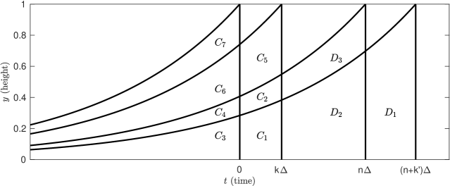
Figure 5: Illustration of the decomposition of the four trawl sets $A_{0},A_{k\Delta},A_{n\Delta},A_{(n+k^{\prime})\Delta}$.

∎

Remark A.1.

Note that in the case of a Poisson Lévy basis (Example 2.1 in the main article), we have $\tilde{\nu}=\nu$, $\tilde{\eta}(1)=1$, and $\tilde{\eta}(c)=0$ for $c\neq 1$. Further, in the case of $d$ being a Gamma trawl function (Example 2.5), it is straightforward to show that $a_{1}=a_{2}=a_{4}=0$ and $a_{3}=1$. For this specification, the limit in the proof of Lemma A.1 simplifies somewhat. Indeed, in this case, Equation (A.7) yields

$$G(x_{1},x_{2},x_{3},x_{4};k,k^{\prime},\theta)=\nu\left(\frac{f_{k}(x_{1}-1,x_{2}-1;\theta)}{f_{k}(x_{1},x_{2};\theta)}-1\right)\left(\frac{f_{k^{\prime}}(x_{3}-1,x_{4}-1;\theta)}{f_{k^{\prime}}(x_{3},x_{4};\theta)}-1\right).$$

Lemma A.2.

In the setting of the proof of Lemma A.1, we have the following two-part result.

(First part) There exists a constant $\tilde{\nu}>0$, such that

$$1-\prod_{j=1}^{4}\mathbb{P}_{\theta}\left(L(C_{j})=0\right)=\tilde{\nu}Leb(A_{k\Delta}\cap A_{n\Delta})+o\left(Leb(A_{k\Delta}\cap A_{n\Delta})\right),$$

as $n\rightarrow\infty$.

(Second part) There exists a non-negative function $\tilde{\eta}$, concentrated on the integers, such that, for $c_{j}\neq 0$,

$$\mathbb{P}_{\theta}\left(L(C_{j})=c_{j}\right)=\tilde{\eta}(c_{j})\tilde{\nu}Leb(C_{j})e^{-\tilde{\nu}Leb(C_{j})}+o\left(Leb(C_{j})\right),$$

as $n\rightarrow\infty$, while

$$\mathbb{P}_{\theta}\left(L(C_{j})=0\right)=e^{-\tilde{\nu}Leb(C_{j})}+o\left(Leb(C_{j})\right),$$

as $n\rightarrow\infty$.

Proof of Lemma A.2.

The proof of the lemma relies on the alternative representation of the Lévy basis $L$ given at the start of the Appendix, see Equation (A.1).

(Proof of second part) Note that since $\eta(0)=0$, we have $\mathbb{P}_{\theta}\left(Y_{i}=0\right)=0$. Using this in the setup of Lemma A.1, we get, from Equations (A.1) and (A.2),

$$\mathbb{P}_{\theta}\left(L(C_{j})=0\right) =e^{-\tilde{\nu}Leb(C_{j})}+\sum_{q=2}^{\infty}\mathbb{P}_{\theta}\left(\sum_{i=1}^{q}Y_{i}=x\right)\mathbb{P}_{\theta}(\tilde{N}(C_{j})=q)$$

$$=e^{-\tilde{\nu}Leb(C_{j})}+o\left(Leb(C_{j})\right),$$

as $n\rightarrow\infty$, while for $c_{j}\neq 0$,

$$\mathbb{P}_{\theta}\left(L(C_{j})=c_{j}\right) =\mathbb{P}_{\theta}\left(Y_{1}=c_{j}\right)\mathbb{P}_{\theta}(\tilde{N}(C_{j})=1)+\sum_{q=2}^{\infty}\mathbb{P}_{\theta}\left(\sum_{i=1}^{q}Y_{i}=x\right)\mathbb{P}_{\theta}(\tilde{N}(C_{j})=q)$$

$$=\tilde{\eta}(c_{j})\tilde{\nu}Leb(C_{j})e^{-\tilde{\nu}Leb(C_{j})}+o\left(Leb(C_{j})\right),$$

as $n\rightarrow\infty$. This proves the second part of the lemma.

(Proof of first part) As for the first part, use Equations (A.1) and (A.2) to write

$$\prod_{j=1}^{4}\mathbb{P}_{\theta}\left(L(C_{j})=0\right) =e^{-\tilde{\nu}\sum_{j=1}^{4}Leb(C_{j})}+o\left(\sum_{j=1}^{4}Leb(C_{j})\right)$$

$$=e^{-\tilde{\nu}Leb(A_{n\Delta}\cap A_{k\Delta})}+o\left(Leb(A_{n\Delta}\cap A_{k\Delta})\right)$$

$$=1-\tilde{\nu}Leb(A_{n\Delta}\cap A_{k\Delta})+o\left(Leb(A_{n\Delta}\cap A_{k\Delta})\right),$$

as $n\rightarrow\infty$, where we in the last line Taylor expanded the exponential function. This proves the first part of the lemma.

∎

Proof of Theorem 3.4.

With similar calculations to those used in the proof of Theorem 3.3, we can write

$$n^{H/2}(\hat{\theta}-\theta_{0})=-\left(\frac{1}{n}\frac{\partial}{\partial\theta^{\prime}}s_{n}(\bar{\theta})\right)^{-1}n^{H/2-1}s_{n}(\theta_{0}).$$

We again have that $-\frac{1}{n}\frac{\partial}{\partial\theta}s_{n}(\bar{\theta})^{\prime}\stackrel{{\scriptstyle\mathbb{P}}}{{\rightarrow}}H(\theta_{0})$ as $n\rightarrow\infty$. As in the proof of Theorem 3.3, we can write

$$Var\left(s_{n}(\theta_{0})\right)=A_{1,n}+A_{2,n},$$

where $A_{1,n}$ is $O(n)$. Further, Lemma A.1 implies that

$$A_{2,n}=O(n^{2}Leb(A_{n\Delta}\cap A_{0})),$$

as $n\rightarrow\infty$. Equation (2.5) along with the condition on $\rho$ imposed in the theorem thus yields

$$A_{2,n}=O(n^{2}L_{\infty}(n\Delta)n^{-H}),$$

as $n\rightarrow\infty$. Using this, we get that, for all $\epsilon>0$,

$$n^{H-2\pm 2\epsilon}Var\left(s_{n}(\theta_{0})\right)=O(n^{H-1\pm 2\epsilon})+O(L_{\infty}(n\Delta)n^{\pm 2\epsilon}),$$ (A.8)

as $n\rightarrow\infty$. Finally, we recall the so-called Potter bounds for slowly varying functions: Since $L_{\infty}$ is a slowly varying function, for all $\epsilon>0$ it holds that (Bingham et al. 1989, Theorem 1.5.6(ii))

$$L_{\infty}(n\Delta)n^{\epsilon}\rightarrow\infty\quad\textnormal{ and }\quad L_{\infty}(n\Delta)n^{-\epsilon}\rightarrow 0,$$

as $n\rightarrow\infty$. Combining the Potter bounds with (A.8) yields the required results. ∎

Proof of Theorem 3.5.

Set, for simplicity, $K=1$. From the proof of Theorem 3.3, it is clear that the asymptotic behaviour of $\hat{\nu}^{CL}$ is governed by the asymptotic behaviour of the score function

$$s_{n}(\nu_{0}) =\sum_{i=1}^{n}\left.\frac{\partial}{\partial\nu}\log f(X_{i\Delta},X_{(i+1)\Delta})\right|_{\nu=\nu_{0}}=\sum_{i=1}^{n}\left.\frac{1}{f(X_{i\Delta},X_{(i+1)\Delta})}\frac{\partial}{\partial\nu}f(X_{i\Delta},X_{(i+1)\Delta})\right|_{\nu=\nu_{0}}.$$ (A.9)

Let $B$ be a Borel set. Since $L^{\prime}\sim Poi(\nu)$, we have

$$\mathbb{P}\left(L(B)=x\right)=\frac{[\nu Leb(B)]^{x}\exp(-\nu Leb(B))}{x!},\quad x=0,1,\ldots.$$

Hence,

$$\frac{\partial}{\partial\nu}\mathbb{P}\left(L(B)=x\right)=\left(x\nu^{-1}-Leb(B)\right)\mathbb{P}\left(L(B)=x\right),\quad x=0,1,\ldots.$$

Using this, along with Proposition 3.1, it is straightforward to show that

$$\frac{1}{f(X_{(i+1)\Delta},X_{i\Delta})}\frac{\partial}{\partial\nu}f(X_{i\Delta},X_{(i+1)\Delta}) =\nu^{-1}(X_{(i+1)\Delta}+X_{i\Delta})-C_{i}-D_{i}$$ (A.10)

where

$$C_{i} =\frac{\nu^{-1}}{f(X_{(i+1)\Delta},X_{i\Delta})}\sum_{c=0}^{\min(X_{i\Delta},X_{(i+1)\Delta})}c\cdot P(L(A_{(i+1)\Delta})=X_{(i+1)\Delta},L(A_{i\Delta})=X_{i\Delta},(L(A_{i\Delta}\cap A_{(i+1)\Delta})=c)$$

$$=\nu^{-1}\sum_{c=0}^{\min(X_{i\Delta},X_{(i+1)\Delta})}c\cdot P((L(A_{i\Delta}\cap A_{(i+1)\Delta})=c|L(A_{(i+1)\Delta})=X_{(i+1)\Delta},L(A_{i\Delta})=X_{i\Delta})$$

$$=\nu^{-1}\mathbb{E}[L(A_{i\Delta}\cap A_{(i+1)\Delta})|X_{i\Delta},X_{(i+1)\Delta}]$$

$$=\nu^{-1}\mathbb{E}[L(A_{i+k})-L(A_{(i+1)\Delta}\setminus A_{i\Delta})|X_{i\Delta},X_{(i+1)\Delta}]$$

$$=\nu^{-1}\mathbb{E}[X_{(i+1)\Delta}-L(A_{(i+1)\Delta}\setminus A_{i\Delta})|X_{i\Delta},X_{(i+1)\Delta}]$$

$$=\nu^{-1}\left(X_{(i+1)\Delta}-\mathbb{E}[L(A_{(i+1)\Delta}\setminus A_{i\Delta})|X_{i\Delta},X_{(i+1)\Delta}]\right)$$ (A.11)

and

$$D_{i} =Leb(A_{(i+1)\Delta}\setminus A_{i\Delta})+Leb(A_{i\Delta}\setminus A_{(i+1)\Delta})+Leb(A_{i\Delta}\cap A_{(i+1)\Delta})$$

$$=Leb(A)+Leb(A_{(i+1)\Delta}\setminus A_{i\Delta}).$$ (A.12)

Define $U_{i}:=\mathbb{E}[L(A_{(i+1)\Delta}\setminus A_{i\Delta})|X_{i\Delta},X_{(i+1)\Delta}]$, $i=1,2,\ldots,n$. Recall that $\mathbb{E}[L(B)]=\nu Leb(B)$ from which we deduce that

$$\mathbb{E}[X_{i\Delta}]=\nu Leb(A),\quad\textnormal{ and }\quad\mathbb{E}[U_{i}]=\nu Leb(A_{(i+1)\Delta}\setminus A_{i\Delta}).$$

Using the above and Equations (A.10)–(A.11) in Equation (A.9), we get

$$s_{n}(\nu_{0})=\nu_{0}^{-1}S_{n}(X)+\nu_{0}^{-1}S_{n}(U),$$

Using arguments similar to those in the proof of Theorem 3.3, the result now follows from Theorem 3.6.

∎

Before we provide the proof of Theorem 3.6, we will need the following two lemmas. For two sequences $a_{n},b_{n}$, we will write “$a_{n}\sim b_{n}$” if $a_{n}/b_{n}$ tends to a non-zero constant as $n\rightarrow\infty$.

Lemma A.3.

Let Assumption 3.4 hold and define the sets

$$B_{i,k}=\{(x,s):(i-1)\Delta\leq s\leq i\Delta,d(s-(k+1)\Delta)\leq x<d(s-k\Delta)\},$$ (A.13)

for $i=1,2,\ldots,n$ and $k\in\mathbb{N}$. Then, for all $i=1,2,\ldots,n$,

$$Leb(B_{i,k})=\Delta^{2}d^{\prime}(-(k-i+1+r_{2})\Delta),$$

where $r_{2}=r_{2}(i,k)\in(-1,1)$. In particular,

$$Leb(B_{1,N})\sim g_{2}(N)N^{-H-2},\quad N\rightarrow\infty,$$

and

$$\sum_{k=1}^{\infty}kLeb(B_{1,k})<\infty.$$

Proof of Lemma A.3.

Fix $i\in\{1,2,\ldots,n\}$ and $k\geq 1$. Using the mean value theorem twice, we may write,

$$Leb(B_{i,k}) =\int_{(i-1)\Delta}^{i\Delta}\left(d(x-k\Delta)-d(x-(k+1)\Delta)\right)dx$$

$$=\Delta\int_{(i-1)\Delta}^{i\Delta}d^{\prime}(x-(k+r_{1})\Delta)dx$$

$$=\Delta[d(-(k+r_{1}-i)\Delta)-d(-(k+r_{1}-i+1)\Delta)]$$

$$=\Delta^{2}d^{\prime}(-(k-i+1+r_{2})\Delta),$$

where $r_{1}\in(0,1)$ and $r_{2}\in(-1,1)$, which proves the first part of the lemma. Note that $r_{1}$ and $r_{2}$ will in general depend on $k$ and $i$, but we will suppress this for ease of notation. The latter parts of the lemma now follow from Assumption 3.4. ∎

Lemma A.4.

Let Assumption 3.4 hold and define the sets

$$\bar{B}_{1,k}=\cup_{j=k+1}^{\infty}B_{1,j},\qquad k\in\mathbb{N}.$$ (A.14)

Then,

$$Leb(\bar{B}_{1,N}) =\int_{0}^{\Delta}d(s-(N+1)\Delta)ds\sim g_{1}(N)N^{-H-1},$$

as $N\rightarrow\infty$. In particular, using also Lemma A.3,

$$\sum_{k=1}^{\infty}kLeb(B_{1,k})^{1/2}Leb(\bar{B}_{1,k})<\infty.$$

Proof of Lemma A.4.

Using a change-of-variables, Assumption 3.4, Karamata’s theorem, the mean value theorem, and standard properties of slowly varying functions, we get

$$Leb(\bar{B}_{1,N}) =\int_{0}^{\Delta}d(s-(N+1)\Delta)ds$$

$$=\int_{N\Delta}^{(N+1)\Delta}d(-y)dy$$

$$=\int_{N\Delta}^{\infty}g_{1}(y)y^{-H-1}dy-\int_{(N+1)\Delta}^{\infty}g_{1}(y)y^{-H-1}dy$$

$$\sim\frac{1}{H}g_{1}(N\Delta)(N\Delta)^{-H}-\frac{1}{H}g_{1}((N+1)\Delta)((N+1)\Delta)^{-H}$$

$$=\frac{\Delta^{-H}}{H}g_{1}(N\Delta)\left(N^{-H}-\frac{g_{1}((N+1)\Delta)}{g_{1}(N\Delta)}(N+1)^{-H}\right)$$

$$=\frac{\Delta^{-H}}{H}g_{1}(N\Delta)\left(N^{-H}-(N+1)^{-H}-\left(\frac{g_{1}((N+1)\Delta)}{g_{1}(N\Delta)}-1\right)(N+1)^{-H}\right)$$

$$\sim\frac{\Delta^{-H}}{H}g_{1}(N\Delta)\left(N^{-H}-(N+1)^{-H}\right)$$

$$=\Delta^{-H}g_{1}(N\Delta)(N+r_{1})^{-H-1}$$

$$\sim g_{1}(N\Delta)N^{-H-1},$$

$$\sim g_{1}(N)N^{-H-1},$$

as $N\rightarrow\infty$, where $r_{1}\in(0,1)$. The latter parts of the lemma now follow from Assumption 3.4. ∎

Proof of Theorem 3.6.

Suppose for simplicity that $L^{\prime}\sim Poi(\nu)$ for some $\nu>0$. The general case follows along similar lines to the proof in the Poisson case, using the compound Poisson representation of the IVT process as presented above.

We follow the strategy of the proof outlined in Theorem 2 of Doukhan et al. (2019), adapted to our purposes. First, define the sequence of random variables

$$Z_{i} =Z_{i\Delta}=L(A_{i\Delta}\setminus A_{(i-1)\Delta})+\sum_{j=1}^{\infty}L((A_{i\Delta}\cap A_{(i-j)\Delta})\setminus A_{(i-j-1)\Delta}+(0,j\Delta)),\quad i=1,2,\ldots,n,$$

where the sum converges almost surely by Kolmogorov’s three-series theorem. Note that

$$(A_{i\Delta}\cap A_{(i-j)\Delta})\setminus A_{(i-j-1)\Delta}=\{(x,s):(i-j-1)\Delta<s\leq(i-j)\Delta,0\leq d(s-i\Delta)\},$$

and, hence, applying a time shift of $j\Delta$ leads to

$$(A_{i\Delta}\cap A_{(i-j)\Delta})\setminus A_{(i-j-1)\Delta}+(0,j\Delta)\\ =\{(x,s):(i-1)\Delta<s\leq i\Delta,0\leq d(s-(i+j)\Delta)\}.$$

We observe that we can write $Z_{i}$ as a sum of independent variables,

$$Z_{i} =\sum_{k=1}^{\infty}kL(B_{i,k}),$$

where $B_{i,k}$ are disjoint sets, given as in Equation (A.14). The construction of $Z_{1}$, and the decomposition into independent variables, are illustrated in Figure 6. Note furthermore that, by construction, the sequence $\{Z_{i}\}_{i=1}^{\infty}$ is iid. Let $S_{n}(\cdot)$ denote the de-meaned partial sums of a process, e.g. $S_{n}(X)=\sum_{i=1}^{n}(X_{i}-\mathbb{E}[X_{i}])$. Here we use the short-hand notation that $X_{i}=X_{i\Delta}$. Our aim is to show that

1. $\mathbb{P}(Z_{1}>y)\sim g(y)y^{-H-1}$, as $y\rightarrow\infty$, where $g$ is a slowly varying function.

2. $\mathbb{E}[|S_{n}(X)-S_{n}(Z)|]=o(n^{1/(H+1)})$, as $n\rightarrow\infty$.

Indeed, the result of the present theorem follows from (i) and (ii). To see this, note that (i) implies that (Ibragimov & Linnik 1971, Theorem 2.6.7)

$$n^{-1/(H+1)}S_{n}(Z)\stackrel{{\scriptstyle(d)}}{{\rightarrow}}L_{1+H},\quad n\rightarrow\infty,$$

where $L_{1+H}$ is an $(1+H)$-stable random variable with characteristic function as given in Equation (3.6). Secondly, (ii) now implies that

$$n^{-1/(H+1)}S_{n}(X)=n^{-1/(H+1)}S_{n}(Z)+o_{\mathbb{P}}(1)\stackrel{{\scriptstyle(d)}}{{\rightarrow}}L_{1+H},\quad n\rightarrow\infty,$$

which is what we wanted to show.

We proceed to prove (i). First, let $Z^{*}$ be given by

$$Z^{*}=\sum_{k=1}^{\infty}kI(L(B_{1,k})>0),$$

where $I(A)$ is the indicator of the set $A$. Note that $Z_{1}\geq Z^{*}\geq 0$. Second, define $Z^{**}=Z_{1}-Z^{*}$. Let $g$ be a slowly varying function. As in Doukhan et al. (2019), we prove that (a) $\mathbb{P}(Z^{*}>y)=g(y)y^{-H-1}+o(y^{-H-1})$ and (b) $\mathbb{P}(Z^{**}>y)=o(y^{-H-1})$ as $y\rightarrow\infty$, which allows us to deduce (i), i.e. $\mathbb{P}(Z_{1}>y)\sim g(y)y^{-H-1}$ as $y\rightarrow\infty$.

To prove (a), define the random variables

$$Z_{1}^{*} :=\sum_{k=1}^{\infty}kI(L(B_{1,k})>0)I(L(\bar{B}_{1,k})=0),$$

$$Z_{2}^{*} :=\sum_{k=1}^{\infty}kI(L(B_{1,k})>0)I(L(\bar{B}_{1,k})=1),$$

where, as before,

$$\bar{B}_{1,k}=\{(x,s):0\leq s\leq\Delta,0\leq x<d(s-(k+1)\Delta)\}=\cup_{j=k+1}^{\infty}B_{1,j}.$$ (A.15)

The intuition is that $Z_{1}^{*}$ takes the value $k$ if there is an observation in $B_{1,k}$ but not in $B_{1,k+1},B_{1,k+2},\ldots$, while $Z_{2}^{*}$ takes the value $k$ if there is an observation in $B_{1,k}$ and precisely one observation in $B_{1,k+1},B_{1,k+2},\ldots$. Note that $Z^{*}\geq Z_{1}^{*}+Z_{2}^{*}\geq 0$. Define, analogously to above $Z_{3}^{*}=Z^{*}-Z_{1}^{*}-Z_{2}^{*}$, which is $Z^{*}$ with the two largest “points” removed. We prove that (a’) $\mathbb{P}(Z_{1}^{*}>y)\sim g(y)y^{-H-1}$ and (b’) $\mathbb{P}(Z_{2}^{*}>y)=o(y^{-H-1})$ and $\mathbb{P}(Z_{3}^{*}>y)=o(y^{-H-1})$ as $y\rightarrow\infty$, which allows us to deduce (a), i.e. $\mathbb{P}(Z^{*}>y)\sim g(y)y^{-H-1}$ as $y\rightarrow\infty$. As noted in Doukhan et al. (2019), to prove (a’), we only need to prove $\mathbb{P}(Z_{1}^{*}>N)\sim g(N)N^{-H-1}+o(N^{-H-1})$ for $N\rightarrow\infty$, where $N\in\mathbb{N}$. Let therefore $N\in\mathbb{N}$. We get, using Lemma A.4 and the fact that $L^{\prime}\sim Poi(\nu)$,

$$\mathbb{P}(Z_{1}^{*}>N) =\mathbb{P}\left(\sum_{k=1}^{\infty}kI(L(B_{1,k})>0)I(L(\bar{B}_{1,k})=0)>N\right)$$

$$=\mathbb{P}\left(L(\bar{B}_{1,N})>0\right)$$

$$=1-\mathbb{P}\left(L(\bar{B}_{1,N})=0\right)$$

$$=1-e^{-\nu Leb(\bar{B}_{1,N})}$$

$$=Leb(\bar{B}_{1,N})+o(Leb(\bar{B}_{1,N}))$$

$$\sim g_{1}(N)N^{-H-1},$$

as $N\rightarrow\infty$.

To prove (b’), note that, by Lemma A.4,

$$\mathbb{P}(Z_{2}^{*}>N) =\mathbb{P}\left(\sum_{k=1}^{\infty}kI(L(B_{1,k})>0)I(L(\bar{B}_{1,k})=1)>N\right)$$

$$=\mathbb{P}\left(L(\bar{B}_{1,N})>1)\right)$$

$$=1-\mathbb{P}\left(L(\bar{B}_{1,N})=0\right)-\mathbb{P}\left(L(\bar{B}_{1,N})=1)\right)$$

$$=1-e^{-\nu Leb(\bar{B}_{1,N})}-\nu Leb(\bar{B}_{1,N})e^{-\nu Leb(\bar{B}_{1,N})}$$

$$\leq\nu Leb(\bar{B}_{1,N})-\nu Leb(\bar{B}_{1,N})e^{-\nu Leb(\bar{B}_{1,N})}$$

$$=\nu Leb(\bar{B}_{1,N})(1-e^{-\nu Leb(\bar{B}_{1,N})})$$

$$\leq\nu^{2}Leb(\bar{B}_{1,N})^{2}$$

$$\sim g_{1}(N)^{2}N^{-2-2H}$$

$$=o(N^{-1-H}),$$

as $N\rightarrow\infty$, by Lemma A.4. To show that $\mathbb{P}(Z_{3}^{*}>y)=o(y^{-H-1})$ as $y\rightarrow\infty$, we show that $Z_{3}^{*}$ is bounded in $L^{2}$. Let $\epsilon\in(0,H)$. Using Minkowski’s inequality, the independence of $L(B_{1,k})$ and $L(\bar{B}_{1,k})$, and Lemmas A.3 and A.4, we get

$$\mathbb{E}[(Z_{3}^{*})^{2}]^{1/2} =\mathbb{E}\left[\left(Z^{*}-Z_{1}^{*}-Z_{2}^{*}\right)^{2}\right]^{1/2}$$

$$=\mathbb{E}\left[\left(\sum_{k=1}^{\infty}kI(L(B_{1,k})>0)\left(1-I(L(\bar{B}_{1,k})=0)-I(L(\bar{B}_{1,k})=1)\right)\right)^{2}\right]^{1/2}$$

$$\leq\sum_{k=1}^{\infty}\mathbb{E}\left[k^{2}I(L(B_{1,k})>0)^{2}\left(1-I(L(\bar{B}_{1,k})=0)-I(L(\bar{B}_{1,k})=1)\right)^{2}\right]^{1/2}$$

$$=\sum_{k=1}^{\infty}k\mathbb{E}\left[I(L(B_{1,k})>0)I(L(\bar{B}_{1,k})>1)\right]^{1/2}$$

$$=\sum_{k=1}^{\infty}k\mathbb{P}(L(B_{1,k})>0)^{1/2}\mathbb{P}(L(\bar{B}_{1,k})>1)^{1/2}$$

$$=\sum_{k=1}^{\infty}k\left(1-\mathbb{P}(L(B_{1,k})=0)\right)^{1/2}\left(1-\mathbb{P}(L(\bar{B}_{1,k})=0)-\mathbb{P}(L(\bar{B}_{1,k})=1)\right)^{1/2}$$

$$=\sum_{k=1}^{\infty}k\left(1-\exp(-\nu Leb(B_{1,k})\right)^{1/2}\left(1-\exp(-\nu Leb(\bar{B}_{1,k}))-\nu Leb(\bar{B}_{1,k})\exp(-\nu Leb(\bar{B}_{1,k}))\right)^{1/2}$$

$$\leq\sum_{k=1}^{\infty}k\nu^{1/2}Leb(B_{1,k})^{1/2}\left(\nu Leb(\bar{B}_{1,k})-\nu Leb(\bar{B}_{1,k})\exp(-\nu Leb(\bar{B}_{1,k}))\right)^{1/2}$$

$$=\sum_{k=1}^{\infty}k\nu^{1/2}Leb(B_{1,k})^{1/2}\nu^{1/2}Leb(\bar{B}_{1,k})^{1/2}\left(1-\exp(-\nu Leb(\bar{B}_{1,k}))\right)^{1/2}$$

$$\leq\nu^{3/2}\sum_{k=1}^{\infty}kLeb(B_{1,k})^{1/2}Leb(\bar{B}_{1,k})$$

$$<\infty,$$

where we used, repeatedly, that $1-e^{-x}\leq x$.

To prove (b), we show that $Z^{**}$ is bounded in $L^{2}$. We utilize the assumption that $L^{\prime}\sim Poi(\nu)$, which implies that $L(B)=L(B)$ for all Borel sets $B$. This allows us to write

$$Z_{1} =\sum_{k=1}^{\infty}kL(B_{1,k})$$

$$=\sum_{k=1}^{\infty}kL(B_{1,k})I(L(B_{1,k})=1)+\sum_{k=1}^{\infty}kL(B_{1,k})I(L(B_{1,k})>1)$$

$$=\sum_{k=1}^{\infty}kI(L(B_{1,k})=1)+\sum_{k=1}^{\infty}kL(B_{1,k})I(L(B_{1,k})>1),$$

and

$$Z_{1}^{*} =\sum_{k=1}^{\infty}kI(L(B_{1,k})>0)$$

$$=\sum_{k=1}^{\infty}kI(L(B_{1,k})=1)+\sum_{k=1}^{\infty}kI(L(B_{1,k})>1).$$

We deduce that

$$Z_{1}^{**} =Z_{1}-Z_{1}^{*}$$

$$=\sum_{k=1}^{\infty}kL(B_{1,k})I(L(B_{1,k})>1)-\sum_{k=1}^{\infty}kI(L(B_{1,k})>1)$$

$$=\sum_{k=1}^{\infty}kI(L(B_{1,k})>1)(L(B_{1,k})-1)$$

$$\leq\sum_{k=1}^{\infty}kI(L(B_{1,k})>1)L(B_{1,k}).$$

Using this and then Minkowski’s inequality, we may write

$$\mathbb{E}[(Z_{1}^{**})^{2}]^{1/2} \leq\mathbb{E}[(\sum_{k=1}^{\infty}kI(L(B_{1,k})>1)L(B_{1,k}))^{2}]^{1/2}$$

$$\leq\sum_{k=1}^{\infty}\mathbb{E}[k^{2}I(L(B_{1,k})>1)L(B_{1,k})^{2}]^{1/2}$$

$$=\sum_{k=1}^{\infty}k\mathbb{E}[I(L(B_{1,k})>1)L(B_{1,k})^{2}]^{1/2}$$

$$=\sum_{k=1}^{\infty}k\mathbb{E}[\sum_{j=2}^{\infty}(I(L(B_{1,k})=j))L(B_{1,k})^{2}]^{1/2}$$

$$=\sum_{k=1}^{\infty}k\left(\sum_{j=2}^{\infty}\mathbb{E}[I(L(B_{1,k})=j)j^{2}]\right)^{1/2}$$

$$=\sum_{k=1}^{\infty}k\left(\sum_{j=2}^{\infty}\mathbb{P}(I(L(B_{1,k})=j)j^{2}\right)^{1/2}$$

$$=\sum_{k=1}^{\infty}k\left(\sum_{j=2}^{\infty}\frac{(\nu Leb(B_{1,k}))^{j}e^{-\nu Leb(B_{1,k})}}{j!}j^{2}\right)^{1/2}$$

$$=\sum_{k=1}^{\infty}k\left(\nu^{2}Leb(B_{1,k})^{2}\sum_{j=2}^{\infty}\frac{(\nu Leb(B_{1,k}))^{j-2}e^{-\nu Leb(B_{1,k})}}{j!}j^{2}\right)^{1/2}$$

$$=\sum_{k=1}^{\infty}k\left(\nu^{2}Leb(B_{1,k})^{2}\sum_{j=0}^{\infty}\frac{(\nu Leb(B_{1,k}))^{j}e^{-\nu Leb(B_{1,k})}}{(j+2)!}(j+2)^{2}\right)^{1/2}$$

$$=\sum_{k=1}^{\infty}k\left(\nu^{2}Leb(B_{1,k})^{2}\sum_{j=0}^{\infty}\frac{(\nu Leb(B_{1,k}))^{j}e^{-\nu Leb(B_{1,k})}}{j!}\frac{(j+2)}{(j+1)}\right)^{1/2}$$

$$\leq\sum_{k=1}^{\infty}k\left(\nu^{2}Leb(B_{1,k})^{2}\sum_{j=0}^{\infty}2\frac{(\nu Leb(B_{1,k}))^{j}e^{-\nu Leb(B_{1,k})}}{j!}\right)^{1/2}$$

$$=\sqrt{2}\nu\sum_{k=1}^{\infty}kLeb(B_{1,k})$$

$$<\infty,$$

by Lemma A.3.

We now prove (ii). Let $\kappa_{1}=\mathbb{E}[L^{\prime}]$. Note first that

$$\mathbb{E}[Z_{1}] =\kappa_{1}\left(Leb(A_{i\Delta}\setminus A_{(i-1)\Delta})+\sum_{j=1}^{\infty}Leb((A_{i\Delta}\cap A_{(i-j)\Delta})\setminus A_{(i-j-1)}+(0,j\Delta))\right)$$

$$=\kappa_{1}Leb(A)$$

$$=\mathbb{E}[X_{1}],$$

and

$$X_{i}=L(A_{i\Delta}\setminus A_{(i-1)\Delta})+\sum_{j=1}^{\infty}L(A_{i\Delta}\cap A_{(i-j)\Delta}),\quad i=1,2,\ldots,n,$$

see Figure 6 for an illustration of these results. Now, following again Doukhan et al. (2019), we can use this to write

$$S_{n}(X)-S_{n}(Z) =\sum_{i=1}^{n}X_{i}-\sum_{i=1}^{n}Z_{i}$$

$$=\sum_{i=1}^{n}X_{i}-\sum_{i=1}^{n}Z_{i}$$

$$=\sum_{i=1}^{n}\left(L(A_{i\Delta}\setminus A_{(i-1)\Delta})+\sum_{j=1}^{\infty}L((A_{i\Delta}\cap A_{(i-j)\Delta})\setminus A_{(i-j-1)\Delta})\right)$$

$$-\sum_{i=1}^{n}\left(L(A_{i\Delta}\setminus A_{(i-1)\Delta})+\sum_{j=1}^{\infty}L((A_{i\Delta}\cap A_{(i-j)\Delta})\setminus A_{(i-j-1)\Delta}+(0,j\Delta))\right)$$

$$=R_{n}^{\prime}-R_{n}^{\prime\prime},$$

where

$$R_{n}^{\prime} =\sum_{i=1}^{n}L(A_{0}\cap A_{i\Delta}),$$

and

$$R_{n}^{\prime\prime} =\sum_{i=1}^{n}\sum_{k=1}^{\infty}kL(B_{n+1-i,i+k}).$$

Let $\epsilon\in(0,H^{2}/2)$. By Karamata’s Theorem, Assumption 3.4, and properties of slowly varying functions, we have

$$\mathbb{E}[R_{n}^{\prime}] =\mathbb{E}[L^{\prime}]\sum_{k=1}^{n}Leb(A_{0}\cap A_{k\Delta})$$

$$=\kappa_{1}\sum_{k=1}^{n}\int_{k\Delta}^{\infty}d(-x)dx$$

$$\sim\sum_{k=1}^{n}g_{1}(k)k^{-H}$$

$$\sim O(n^{1-H+\epsilon}),$$

as $n\rightarrow\infty$. Note that since $\epsilon<\frac{H^{2}}{2}$, then $1-H+\epsilon<\frac{1}{H+1}$, proving that $\mathbb{E}[R_{n}^{\prime}]=o(n^{1/(H+1)})$. Similarly, using Lemma A.4,

$$\mathbb{E}[R_{n}^{\prime\prime}] =\kappa_{1}\sum_{i=1}^{n}\sum_{k=1}^{\infty}kLeb(B_{n+1-i,i+k})$$

$$=\kappa_{1}\sum_{i=1}^{n}\sum_{k=1}^{\infty}kLeb(B_{1,i+k})$$

$$\sim O(n^{1-H+\epsilon}),$$

as $n\rightarrow\infty$. This concludes the proof. ∎

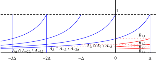
Figure 6: The construction of $Z_{1}=L(A_{\Delta}\setminus A_{0})+\sum_{j=1}^{\infty}L(A_{\Delta}\cap A_{(1-j)\Delta}\setminus A_{(-j)\Delta}+(0,j\Delta))$, and the decomposition into independent variables, $Z_{1}=\sum_{k=1}^{\infty}kL(B_{1,k})$.

Proof of Lemma 4.1.

Using Bayes’ theorem and the unconditional independence of $L(A_{t}\cap A_{t+h})$ and $L(A_{t}\setminus A_{t+h})$, we have for $x\in\mathbb{N}\cup\{0\}$ and $l\in\{0,1,\ldots,x\}$:

$$\mathbb{P}(L(A_{t}\cap A_{t+h})=l|X_{t}=x)=\frac{\mathbb{P}(X_{t}=x|L(A_{t}\cap A_{t+h})=l)\mathbb{P}(L(A_{t}\cap A_{t+h})=l)}{\mathbb{P}(X_{t}=x)}$$

$$=\frac{\mathbb{P}(L(A_{t}\cap A_{t+h})+L(A_{t}\setminus A_{t+h})=x|L(A_{t}\cap A_{t+h})=l)\mathbb{P}(L(A_{t}\cap A_{t+h})=l)}{\mathbb{P}(X_{t}=x)}$$

$$=\frac{\mathbb{P}(L(A_{t}\setminus A_{t+h})=x-l|L(A_{t}\cap A_{t+h})=l)\mathbb{P}(L(A_{t}\cap A_{t+h})=l)}{\mathbb{P}(X_{t}=x)}$$

$$=\frac{\mathbb{P}(L(A_{t}\setminus A_{t+h})=x-l)\mathbb{P}(L(A_{t}\cap A_{t+h})=l)}{\mathbb{P}(X_{t}=x)}.$$

∎

Proof of Proposition 4.1.

Using the conditional law of total probability we obtain the following convolution formula

$$\mathbb{P}(X_{t+h}=x_{t+h}|X_{t}=x_{t})=\mathbb{P}(L(A_{t}\cap A_{t+h})+L(A_{t+h}\setminus A_{t})=x_{t+h}|X_{t}=x_{t})$$

$$=\sum_{c=0}^{\min(x_{t},x_{t+h})}\mathbb{P}(L(A_{t}\cap A_{t+h})+L(A_{t+h}\setminus A_{t})=x_{t+h}|X_{t}=x_{t},L(A_{t}\cap A_{t+h})=c)$$

$$\cdot\mathbb{P}(L(A_{t}\cap A_{t+h})=c|X_{t}=x_{t})$$

$$=\sum_{c=0}^{\min(x_{t},x_{t+h})}\mathbb{P}(L(A_{t+h}\setminus A_{t})=x_{t+h}-c|X_{t}=x_{t},L(A_{t}\cap A_{t+h})=c)\mathbb{P}(L(A_{t}\cap A_{t+h})=c|X_{t}=x_{t})$$

$$=\sum_{c=0}^{\min(x_{t},x_{t+h})}\mathbb{P}(L(A_{t+h}\setminus A_{t})=x_{t+h}-c)\mathbb{P}(L(A_{t}\cap A_{t+h})=c|X_{t}=x_{t}).$$

∎

Supplemental Materials: Inference and forecasting for continuous-time integer-valued trawl processes

Appendix S1 Introduction

This document is structured as follows.

• Section S2 presents a decomposition of trawl processes.

• Section S3 provides the details of a method of moment-based estimation of integer-valued trawl processes so far used in the literature.

• Section S4 describes how the composite likelihood estimator and the corresponding asymptotic covariance matrices can be computed in practice.

• Section S5 presents an expression for the pairwise likelihood for integer-valued processes (not restricted to count data) and discusses a simulation unbiased estimator for the composite likelihood.

• Section S6 contains additional details for the simulation study: Subsection S6.1 describes the simulation setup for the simulation study reported in the main article. Subsections S6.2 and S6.4 present the finite sample results of the MCL estimator and of the model selection procedure, respectively. Section S6.5 repeats the simulation study using different parameter choices.

• Section S7 contains additional details on the empirical study, including details on the data pre-processing, see Subsection S7.1, and additional forecasting results, see Subsection S7.2.

• Sections S8 and S9 present details on various parametric Lévy bases and trawl functions, respectively. These structures might be used in the construction of IVT processes, as illustrated in the main paper.

• Section S10 contains details on how to calculate the gradients for the log-composite likelihood functions implied by most of the parametric IVT processes. These calculations are straightforward to make (although somewhat tedious) and can rather easily be made for other IVT specifications than those considered here. The gradients can be used in the numerical optimization of the composite likelihood functions and are also crucial for implementing the asymptotic theory presented in the main paper. In particular, to estimate the asymptotic variance matrix $V(\theta)$, it is necessary to evaluate the gradient at $\hat{\theta}^{CL}$.

• Section S11 contains some additional technical calculations.

• Section S12 shows that IVT processes are $\theta$-weakly dependent and presents the asymptotic theory for the GMM estimation of the parameters. Section S12.3 contains an analytical comparison of the asymptotic variance of the MCL and GMM estimators in the case of the Poisson-Exponential IVT process.

• Lastly, Section S13 contains brief details on the software packages accompanying the main paper. In particular, we supply software for simulation, estimation (including inference), model selection, and forecasting of IVT processes.

Appendix S2 Trawl process decomposition

When deriving theoretical results for trawl processes, we typically decompose trawl sets at different time points into a partition of disjoint sets. We note that, given a trawl function $d,$ it holds that

$$Leb(A_{t})=Leb(A)=\int_{-\infty}^{0}d(s)ds.$$ (S2.1)

It is also useful to note that for $t\geq s$,

$$Leb(A_{t}\cap A_{s})=Leb(A_{t-s}\cap A)=\int_{-\infty}^{-(t-s)}d(s)ds,$$ (S2.2)

and

$$Leb(A_{t}\setminus A_{s})=Leb(A_{s}\setminus A_{t})=L(A)-Leb(A_{t}\cap A_{s}).$$ (S2.3)

Thus, given a trawl function $d$, it is straightforward to calculate $Leb(A),Leb(A_{t}\cap A_{s})$, and $L(A_{t}\setminus A_{s})$ for all $t\geq s\geq 0$.

Also, we can write, for $0\leq s\leq t$,

$$X_{s} =L(A_{s})=L(A_{s}\cap A_{t})+L(A_{s}\setminus A_{t}),$$

$$X_{t} =L(A_{t})=L(A_{s}\cap A_{t})+L(A_{t}\setminus A_{s}),$$

where the three random variables $L(A_{s}\cap A_{t}),L(A_{s}\setminus A_{t}),L(A_{t}\setminus A_{s})$ are independent since the corresponding sets are disjoint. In Figure S1, we illustrate such a decomposition for $s=3,t=4$.

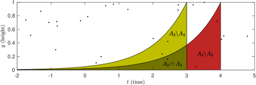
Figure S1: Decomposition of exponential trawl sets at times $s=3,t=4$, super-imposed on a Poisson Lévy basis, with $\nu=5$, on $\mathbb{R}\times[0,1]$. The exponential trawl parameter is set to $\lambda=1$.

Appendix S3 Method-of-moments-based estimation of IVT processes

For a parametric IVT model, let the parameter vector $\theta$ of the model be given by $\theta=(\theta_{d},\theta_{L})$, where $\theta_{d}$ contains the parameters governing the trawl function $d$ and $\theta_{L}$ contains the parameters governing the marginal distribution of the IVT process, as specified by the underlying Lévy seed $L^{\prime}$. For instance, in the case of the Poisson-Exponential IVT process considered above, cf. Figure 1, we would have $\theta_{d}=\lambda$ and $\theta_{L}=\nu$. This section discusses how $\theta_{d}$ and $\theta_{L}$ can be estimated in a two-step procedure using a method-of-moments procedure. It is this procedure that has been used so far in most applied work on IVT processes. Note that we develop the asymptotic theory for the full (one-step) GMM estimation of $\theta$ in Section S12 below.

Because the correlation structure of an IVT process is decoupled from its marginal distribution, the theoretical autocorrelation function of the process will not depend on $\theta_{L}$, and we can thus estimate $\theta_{d}$ in the first step, using the empirical autocorrelations of the data. To be precise, let $\rho_{\theta_{d}}(h)$ be the parametric autocorrelation function as implied by the trawl function $d$, see Equation (2.5), and let $\hat{\rho}(k)$ be the estimate of the empirical autocorrelation of the data at lag $k$. The GMM estimator of $\theta_{d}$ is

$$\hat{\theta}_{d}^{GMM}:=\arg\min_{\theta_{d}\in\Theta_{d}}\sum_{k=1}^{K}\left(\rho_{\theta_{d}}(k)-\hat{\rho}(k)\right)^{2},$$ (S3.1)

where $K\geq 1$ denotes the number of lags to include in the estimation and $\Theta_{d}$ is the parameter space of the trawl parameters in $\theta_{d}$.

For the estimation of the parameters $\theta_{L}$ governing the marginal distribution of the IVT process, recall that the $j$th cumulant $\kappa_{j}$ of $X_{t}$ is given by

$$\kappa_{j}=Leb(A)\cdot\kappa_{j}^{\prime},\quad j=1,2,\ldots,$$

where $\kappa_{j}^{\prime}$ is the $j$th cumulant of the Lévy seed $L^{\prime}$. Using the estimates $\hat{\theta}_{d}^{GMM}$ from the first step, we can estimate the Lebesgue measure of the trawl set as

$$\widehat{Leb(A)}=\int_{0}^{\infty}\hat{d}(-s)ds,$$ (S3.2)

where $\hat{d}(\cdot)$ denotes the estimate of the trawl function implied by the estimated trawl parameters $\hat{\theta}_{d}^{GMM}$. The parameters governing the marginal distribution, $\theta_{L}$, can now be estimated as follows. Let $r$ be the number of elements in $\theta_{L}$ and denote by $\widehat{Leb(A)}$ the estimate of the Lebesgue measure obtained from (S3.2). Estimates of the cumulants, $\hat{\kappa}_{j}$, can be obtained straightforwardly by calculating the empirical cumulants of the data. Let $I_{r}$ be a set of $r$ distinct natural numbers (e.g., the numbers from $1$ to $r$). Now

$$\hat{\kappa}_{j}=\widehat{Leb(A)}\cdot\kappa_{j}^{\prime},\quad j\in I_{r},$$

defines $r$ equations in the $r$ unknowns $\theta_{L}$. GMM estimates of the elements in $\theta_{L}$, $\hat{\theta}_{L}^{GMM}$, can be obtained by solving these $r$ equations. Finally, set $\hat{\theta}^{GMM}:=(\hat{\theta}_{d}^{GMM},\hat{\theta}_{L}^{GMM})$, which is the method-of-moments-based estimator of $\theta$.

Appendix S4 Practical details on feasible inference using the MCL estimator

As shown in Theorem 3.3 of Section 3.1.2, the asymptotic variance of the maximum composite likelihood estimator, $\hat{\theta}_{CL}$ is given by the inverse Godambe information matrix,

$$G(\theta_{0})^{-1}=H(\theta_{0})^{-1}V(\theta_{0})H(\theta_{0})^{-1}.$$

As mentioned, the matrices $H(\theta_{0})$ and $V(\theta_{0})$ can be consistently estimated by

$$\hat{H}(\hat{\theta}^{CL}) =-\frac{1}{n}\frac{\partial}{\partial\theta\partial\theta^{\prime}}l_{CL}(\hat{\theta}^{CL};x)$$

$$=-\frac{1}{n}\sum_{k=1}^{K}\sum_{i=1}^{n-k}\frac{\partial^{2}}{\partial\theta\theta^{\prime}}\log f(x_{(i+k)\Delta},x_{i\Delta};\theta)|_{\theta=\hat{\theta}^{CL}},$$

$$\hat{V}_{HAC}(\hat{\theta}^{CL}) =\hat{\Sigma}_{0}+\sum_{j=1}^{q}\left(1-\frac{j}{q+1}\right)(\hat{\Sigma}_{j}+\hat{\Sigma}_{j}^{\prime}),$$

where

$$\hat{\Sigma}_{j}:=\frac{1}{n}\sum_{k=1}^{K}\sum_{k^{\prime}=1}^{K}\sum_{i=1}^{n-j-k^{\prime}}\frac{\partial}{\partial\theta}\log f(x_{(i+k)\Delta},x_{i\Delta};\theta)|_{\theta=\hat{\theta}^{CL}}\frac{\partial}{\partial\theta^{\prime}}\log f(x_{(i+j+k^{\prime})\Delta},x_{(i+j)\Delta};\theta))|_{\theta=\hat{\theta}^{CL}},$$

and $q\in\mathbb{N}$ is the number of autocorrelation terms to take into account in the HAC estimator. The Hessian, $H(\theta_{0})$, is straightforwardly estimated by the above expression. Indeed, a numerical approximation of this matrix is often directly available as output from the software maximizing the composite likelihood function. We have found that while this estimator $\hat{H}(\hat{\theta}^{CL})$ is quite precise, the HAC estimator $\hat{V}_{HAC}(\hat{\theta}^{CL})$ can be rather imprecise. In practice, we therefore recommend estimating $V(\theta_{0})$ using simulation-based approach; the details are given in the following S4.1.

S4.1 Simulation-based approach to estimating the asymptotic covariance matrix

To obtain a simulation-based estimator of $V(\theta_{0})$, let $B$ denote a positive integer (e.g. $B=500$) and suppose that $\hat{\theta}^{CL}$ is the maximum composite likelihood estimate of $\theta$ from (3.3) when applied to the original data. To estimate $V(\theta_{0})$, do as follows:

1. For $b=1,2,\ldots,B$, simulate $N$ observations of a trawl process $X^{(b)}=\{X^{(b)}_{i}\}_{i=1}^{N}$ with underlying parameters $\hat{\theta}^{CL}$.

2. For $b=1,2,\ldots,B$, use the simulated data $X^{(b)}$ to calculate $s^{(b)}(\hat{\theta}^{CL})=N^{-1/2}\frac{\partial}{\partial\theta}l_{CL}(\hat{\theta}^{CL};X^{(b)})$. The gradient can either be calculated numerically or analytically. Note that the bootstrap data is used to calculate the gradient, but the parameter vector $\hat{\theta}^{CL}$ is the original estimator obtained from the initial (real) data set.

3. Estimate $V(\hat{\theta}^{CL})$ as the sample covariance matrix of the simulated scores $\left\{s^{(b)}(\hat{\theta}^{CL})\right\}_{b=1}^{B}$.

Note that the number of simulated observations, $N$, in Step 1 does not need to equal the number of observations in the original data set, $n$. When $n$ is large, setting $N=n$ can be computationally costly; we found that setting $N=500$ or even $N=100$ provided good results. In our simulation study and in the empirical application we have set $B=N=500$.

S4.2 Feasible inference using parametric bootstrap methods

It is, of course, also possible to side-step the estimation of $G(\theta)^{-1}$ entirely, by considering a “standard” parametric bootstrap approach where the asymptotic variance of the MCL estimator is approximated directly by applying the MCL estimator to $B$ bootstrap samples of IVT processes simulated with parameters $\hat{\theta}^{CL}$. While mechanically simpler to implement than the simulation-based procedure suggested above in Section S4.1, such a parametric bootstrap approach will often be more computationally demanding, since one needs to apply the numerical optimization of the composite likelihood function in each bootstrap replication, whereas the approach suggested in Section S4.1 only requires the evaluation of the composite likelihood once for each $b=1,2,\ldots,B$. Further, the “standard” bootstrap only delivers standard errors of $\hat{\theta}^{CL}$ and can not be used for calculating information criteria (Section 3.2). For these reasons, we do not consider the standard parametric bootstrap approach in this paper. The interested reader should have no trouble implementing it, however.

Appendix S5 Pairwise likelihood for IVT processes and simulation-based likelihood

Proposition 3.1 presented a simple expression for the pairwise PMFs $f(x_{i+k},x_{i};\theta)$ in the case where the underlying Lévy basis is positive. In the general case, i.e. where the Lévy basis is integer-valued, we have, by the law of total probability, that

$$f(x_{i+k}, x_{i};\theta):=\mathbb{P}_{\theta}\left(X_{(i+k)\Delta}=x_{i+k},X_{i\Delta}=x_{i}\right)$$

$$= \sum_{c=-\infty}^{\infty}\mathbb{P}_{\theta}\left(X_{(i+k)\Delta}=x_{i+k},X_{i\Delta}=x_{i}|L(A_{(i+k)\Delta}\cap A_{i\Delta})=c\right)\cdot\mathbb{P}_{\theta}\left(L(A_{(i+k)\Delta}\cap A_{i\Delta})=c\right)$$

$$= \sum_{c=-\infty}^{\infty}\mathbb{P}_{\theta}\left(L(A_{(i+k)\Delta}\setminus A_{i\Delta})=x_{i+k}-c\right)\mathbb{P}_{\theta}\left(L(A_{i\Delta}\setminus A_{(i+k)\Delta})=x_{i}-c\right)$$ (S5.1)

$$\cdot\mathbb{P}_{\theta}\left(L(A_{(i+k)\Delta}\cap A_{i\Delta})=c\right),$$

which can be used for calculating the pairwise likelihood as a function of the parameter vector $\theta$, in the general integer-valued case. When implementing this result in practice, one could truncate the sum in (S5.1) according to some criterion in order to approximate the joint PMF. Truncation can be avoided by resorting to a simulation-based approach, however. The following proposition shows that a simulation unbiased version of the joint PMF exists and that the simulation is, in fact, easy to perform.

Proposition S5.1.

Let $t,s\geq 0$, choose $M\in\mathbb{N}$ and let $C^{(j)}\sim L(A_{t}\cap A_{s})$, $j=1,2,\ldots,M$, be an iid sample. Then

$$\hat{f}(x_{t},x_{s};\theta)=\frac{1}{M}\sum_{j=1}^{M}\mathbb{P}_{\theta}(L(A_{t}\setminus A_{s})=x_{t}-C^{(j)})\mathbb{P}_{\theta}(L(A_{s}\setminus A_{t})=x_{s}-C^{(j)})$$

is a simulation-based unbiased estimator of $f(x_{t},x_{s};\theta)$. We further note that the simulation error

$$\hat{f}(x_{t},x_{s};\theta)-f(x_{t},x_{s};\theta)$$

is, conditional on $x$, stochastically independent for different values of $t$ and $s$. Also, this error converges to zero at rate $\sqrt{M}$ as long as

$$\sum_{c=-\infty}^{\infty}f(x_{t}|c;\theta)^{2}f(x_{s}|c;\theta)^{2}f(x;\theta)<\infty,$$

where $f(c;\theta)=\mathbb{P}_{\theta}(C^{(1)}=c)$ denotes the PMF of $C^{(j)}$, $j=1,2,\ldots,M$, and $f(x_{t}|c;\theta)=\mathbb{P}_{\theta}(X_{t}=x_{t}|L(A_{t}\cap A_{s})=c)$ denotes the conditional PMF of $X_{t}$.

Proof of Proposition S5.1.

Ignoring the dependence on $\theta$ we have

$$f(x_{t},x_{s})=\sum_{c=-\infty}^{\infty}f(x_{t},x_{s}|c)f(c)=\sum_{c=-\infty}^{\infty}f(x_{t}|x_{s},c)f(x_{s}|c)f(c).$$

Since, conditionally on $L(A_{t}\cap A_{s})=c$, $X_{t}$ and $X_{s}$ are independent we have $f(x_{t}|x_{s},c)=f(x_{t}|c)$ and thus

$$f(x_{t},x_{s})=\sum_{c=-\infty}^{\infty}f(x_{t}|c)f(x_{s}|c)f(c),$$

which shows that sampling from $f(c;\theta)$ delivers the quantity we need. The rest of the proposition is obvious. ∎

Proposition S5.1 shows that the simulated CL function is an unbiased estimator of the true CL function. In other words, if we let $U$ denote the vector of uniform random variables behind the simulation of $\{C^{(j)}\}_{j=1}^{M}$ and define

$$\log\mathcal{L}_{U}(\theta;x,u)=\log\mathcal{L}^{(K)}_{U}(\theta;x,u):=\sum_{k=1}^{K}\sum_{i=1}^{n-k}\log\hat{f}(x_{i+k},x_{i};\theta),$$

then $\mathcal{L}_{U}(\theta;x,u)$ is a simulation unbiased estimator for the composite likelihood $\mathcal{L}_{CL}(\theta;x)$. That is

$$\mathcal{L}_{CL}(\theta;x)=\int\mathcal{L}_{U}(\theta;x,u)f_{U}(u)du,$$

where $f_{U}(u)\propto 1$ is the joint density of the uniform random numbers behind all the simulations. It is well known that numerically optimizing a simulated likelihood function (the so-called simulated maximum likelihood approach, see e.g. Lerman and Manski 1981) suffers a number of drawbacks and can be fragile in practice (e.g. Flury and Shephard 2011). However, as a result of the seminal Andrieu et al. (2010), it is feasible to do Markov Chain Monte Carlo (MCMC) when one can unbiasedly simulate the likelihood. As a consequence, it is feasible to perform simulation-based estimation through MCMC, instead of relying on numerical optimization. From an estimation viewpoint, this can be an attractive approach (Flury and Shephard 2011).

Appendix S6 Simulation study

In this section, we provide additional information on the simulation study. We first describe the simulation set-up used for the study which we summarise in the main article in Subsection S6.1.

S6.1 Additional details on the simulation study reported in the main article

In a simulation study, we examine the finite sample properties of the composite likelihood-based estimation procedure and the model selection procedure.

The IVT framework is very flexible and there are many possible choices of data-generating processes (DGPs) to use in the simulation studies. Here, we will consider the six combinations of the two marginal distributions, given in Examples 2.1 and 2.2, and three correlations structures, given in Examples 2.3, 2.4, and 2.5. In other words, we consider the Poisson-Exponential (P-Exp), the Poisson-Inverse Gaussian (P-IG), the Poisson-Gamma (P-Gamma), the Negative Binomial-Exponential (NB-Exp), the Negative Binomial-Inverse Gaussian (NB-IG), and the Negative Binomial-Gamma (NB-Gamma) IVT models. Note that the first model contains two free parameters, the second, third, and fourth models three free parameters, and the fifth and sixth models four free parameters. Since the Lévy bases considered here are non-negative-valued, we will use Proposition 3.1 for the calculation of the pairwise likelihoods.

The parameter values used in the simulation studies are given in Table S1 and the implied marginal distributions and autocorrelation structures are shown in Figure S2. The figure illustrates the difference between the six DGPs: those based on the Poisson Lévy basis have a more concentrated marginal distribution compared to those based on the Negative Binomial Lévy basis; those based on the exponential trawl function have smaller degrees of autocorrelation (memory) than those based on the Inverse Gaussian trawl function, and the Gamma trawl function can exhibit still greater autocorrelation.

The choice of parameter values used in the simulation studies below and given in Table S1 are based on the estimates obtained in the empirical study in Section 6. We have found the finite sample properties of the methods proposed in this paper to be relatively robust to the exact choice of parameter values.

Table S1: Parameter values used in simulation studies

DGP	$\nu$	$m$	$p$	$\lambda$	$\delta$	$\gamma$	$H$	$\alpha$
P-Exp	$17.50$			$1.80$
P-IG	$17.50$				$1.80$	$0.80$
P-Gamma	$17.50$						$1.70$	$0.80$
NB-Exp		$7.50$	$0.70$	$1.80$
NB-IG		$7.50$	$0.70$		$1.80$	$0.80$
NB-Gamma		$7.50$	$0.70$				$1.70$	$0.80$

Parameter values for the six different DGPs used in the simulation studies of Section 5. See Examples 2.1, 2.2, 2.3, 2.4, and 2.5 for details. The value $\nu=mp/(1-p)$ with $m=7.5$ and $p=0.70$ is chosen such that the first moment of the Poisson and Negative Binomial Lévy bases are matched. Marginal distributions and autocorrelation functions implied by these parameter values are shown in Figure S2.

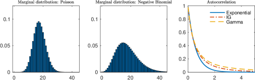
Figure S2: Marginal distributions of the Lévy bases and autocorrelations of the DGPs used in the simulation studies of Section 5. The marginal distribution and autocorrelation structure of IVT processes can be specified independently, resulting in six different DGPs in this setup (P-Exp, P-IG, P-Gamma, NB-Exp, NB-IG, NB-Gamma). See Examples 2.1, 2.2, 2.3, 2.4, and 2.5 for details. The parameter values used to produce the plots are given in Table S1.

S6.2 Finite sample properties of the MCL estimator

Consider $n$ equidistant observations of an IVT process on an equidistant grid of size $0.10$, i.e. $X_{\Delta},X_{2\Delta},\ldots,X_{n\Delta}$ with $\Delta=0.10$. We simulate $500$ Monte Carlo replications of such time series and in each iteration estimate the parameters of the model using the MCL approach of Equation (3.3). For the IVT models based on the exponential trawl function (Example 2.3), we set $K=1$, while we set $K=10$ for the remaining IVT models. In extensive simulation experiments (not reported here), we verified that the results are robust to the choice of $K$.

As mentioned, previous applied work using IVTs has mainly relied on the moment-based estimator. We, therefore, compare the GMM estimation procedure, laid forth in Section S3, with the MCL estimator suggested in this paper. Figure 2 plots the RMSE of the MCL estimator of a given parameter divided by the RMSE of the GMM estimator of the same parameter for the six DGPs of Table S1. Thus, numbers smaller than one indicate that the MCL estimator has a lower RMSE than the GMM estimator and vice versa for numbers larger than one. We see that for most parameters in most of the DGPs, the MCL estimator outperforms the GMM estimator substantially; indeed, in many cases, the RMSE of the MCL estimator is around $50\%$ that of the GMM estimator. The exception seems to be the trawl parameters, i.e. the parameters controlling the autocorrelation structure, in the case of the Gamma and IG trawls, where the GMM estimator occasionally performs on par with the MCL estimator. However, in most cases, it appears that the MCL estimator is able to provide large improvements over the GMM estimator.

S6.2.1 Simulation results supplementing those from the main paper

The simulation results, for various values of $n$, are shown in Tables S2–S7 for the six DGPs of Table S1. We report the median, the median bias, and the root median squared error (RMSE) of the estimator, calculated over the $500$ Monte Carlo replications. The reason for reporting the median, instead of the mean, is that we found that when the number of observations, $n$, is small, the estimation approach will occasionally result in large outliers in few of the Monte Carlo runs, thus skewing the results (this was the case for both the MCL and GMM estimators).

From the tables, we see evidence of the MCL estimator being consistent, i.e. the bias converges towards zero as the number of observations, $n$, grows. As expected, the estimator is most precise for the simpler models, e.g. the Poisson-Exp IVT (Table S2) and somewhat less precise for the more complex models, e.g. the NB-IG model (Table S6) and NB-Gamma model (Table S7).

Table S2: MCL estimation results: Poisson trawl process with exponential trawl function

	$\hat{\nu}$ ($\nu=17.5$)			$\hat{\lambda}$ ($\lambda=1.8$)
$n$	Med.	Bias	RMSE	Med.	Bias	RMSE
$100$	$17.3213$	$-0.1787$	$1.8616$	$1.8351$	$0.0351$	$0.2035$
$250$	$17.4204$	$-0.0796$	$1.1761$	$1.8009$	$0.0009$	$0.1279$
$500$	$17.5179$	$0.0179$	$0.8444$	$1.8012$	$0.0012$	$0.0883$
$1000$	$17.6023$	$0.1023$	$0.6164$	$1.8049$	$0.0049$	$0.0626$
$2000$	$17.5540$	$0.0540$	$0.4538$	$1.8026$	$0.0026$	$0.0476$
$4000$	$17.5099$	$0.0099$	$0.3038$	$1.8000$	$0.0000$	$0.0327$
$8000$	$17.5302$	$0.0302$	$0.2197$	$1.8036$	$0.0036$	$0.0222$

Median (Med.), median bias (Bias) and root median squared error (RMSE) of the MCL estimator with $K=1$. DGP: Poisson-Exponential IVT process. The IVT process $X_{t}$ is simulated on the grid $t=\Delta,2\Delta,\ldots,n\Delta$, with $\Delta=0.10$, see Table S1 for the values of the parameters used in the simulations. Number of Monte Carlo simulations: $500$.

Table S3: CL estimation results: Poisson trawl process with IG trawl function

	$\hat{\nu}$ ($\nu=17.5$)			$\hat{\delta}$ ($\delta=1.8$)			$\hat{\gamma}$ ($\gamma=0.8$)
$n$	Med.	Bias	RMSE	Med.	Bias	RMSE	Med.	Bias	RMSE
$250$	$17.7984$	$0.2984$	$1.8764$	$2.4177$	$0.6177$	$0.9923$	$1.0985$	$0.2985$	$0.5365$
$500$	$17.7749$	$0.2749$	$1.4921$	$2.0205$	$0.2205$	$0.6317$	$0.9306$	$0.1306$	$0.3352$
$1000$	$17.6514$	$0.1514$	$1.0344$	$1.9141$	$0.1141$	$0.4896$	$0.8592$	$0.0592$	$0.2422$
$2000$	$17.5182$	$0.0182$	$0.8090$	$1.8977$	$0.0977$	$0.3413$	$0.8333$	$0.0333$	$0.1864$
$4000$	$17.5273$	$0.0273$	$0.5931$	$1.8120$	$0.0120$	$0.2426$	$0.8051$	$0.0051$	$0.1347$
$8000$	$17.4966$	$-0.0034$	$0.4125$	$1.8072$	$0.0072$	$0.1692$	$0.8030$	$0.0030$	$0.0842$

Median (Med.), median bias (Bias) and root median squared error (RMSE) of the MCL estimator with $K=10$. DGP: Poisson-IG IVT. The IVT process $X_{t}$ is simulated on the grid $t=\Delta,2\Delta,\ldots,n\Delta$, with $\Delta=0.10$, see Table S1 for the values of the parameters used in the simulations. Number of Monte Carlo simulations: $500$.

Table S4: CL estimation results: Poisson trawl process with $\Gamma$ trawl function

	$\hat{\nu}$ ($\nu=17.5$)			$\hat{H}$ ($H=1.7$)			$\hat{\alpha}$ ($\alpha=0.8$)
$n$	Med.	Bias	RMSE	Med.	Bias	RMSE	Med.	Bias	RMSE
$250$	$17.8207$	$0.3207$	$1.8470$	$3.0719$	$1.3719$	$1.4020$	$1.5159$	$0.7159$	$0.7302$
$500$	$17.5946$	$0.0946$	$1.2180$	$2.1831$	$0.4831$	$0.9537$	$1.0463$	$0.2463$	$0.4816$
$1000$	$17.4396$	$-0.0604$	$0.9877$	$1.8563$	$0.1563$	$0.7227$	$0.8914$	$0.0914$	$0.3636$
$2000$	$17.4540$	$-0.0460$	$0.6642$	$1.7807$	$0.0807$	$0.5371$	$0.8406$	$0.0406$	$0.2728$
$4000$	$17.5048$	$0.0048$	$0.4821$	$1.6902$	$-0.0098$	$0.3851$	$0.7784$	$-0.0216$	$0.2004$
$8000$	$17.5612$	$0.0612$	$0.3925$	$1.6433$	$-0.0567$	$0.2464$	$0.7607$	$-0.0393$	$0.1189$

Median (Med.), median bias (Bias) and root median squared error (RMSE) of the MCL estimator with $K=10$. DGP: Poisson-Gamma IVT. The IVT process $X_{t}$ is simulated on the grid $t=\Delta,2\Delta,\ldots,n\Delta$, with $\Delta=0.10$, see Table S1 for the values of the parameters used in the simulations. Number of Monte Carlo simulations: $500$.

Table S5: CL estimation results: NB trawl process with exponential trawl function

	$\hat{m}$ ($m=7.5$)			$\hat{p}$ ($p=0.7$)			$\hat{\lambda}$ ($\lambda=1.8$)
$n$	Med.	Bias	RMSE	Med.	Bias	RMSE	Med.	Bias	RMSE
$100$	$8.9761$	$1.4761$	$2.3850$	$0.6649$	$-0.0351$	$0.0623$	$1.9197$	$0.1197$	$0.2595$
$250$	$7.9680$	$0.4680$	$1.3264$	$0.6872$	$-0.0128$	$0.0353$	$1.8311$	$0.0311$	$0.1431$
$500$	$7.8443$	$0.3443$	$0.9956$	$0.6896$	$-0.0104$	$0.0287$	$1.8202$	$0.0202$	$0.1010$
$1000$	$7.6891$	$0.1891$	$0.6964$	$0.6970$	$-0.0030$	$0.0202$	$1.8106$	$0.0106$	$0.0728$
$2000$	$7.5855$	$0.0855$	$0.5010$	$0.6972$	$-0.0028$	$0.0143$	$1.8001$	$0.0001$	$0.0470$
$4000$	$7.5362$	$0.0362$	$0.3484$	$0.6993$	$-0.0007$	$0.0095$	$1.8013$	$0.0013$	$0.0316$
$8000$	$7.5265$	$0.0265$	$0.2365$	$0.6993$	$-0.0007$	$0.0065$	$1.7994$	$-0.0006$	$0.0251$

Median (Med.), median bias (Bias) and root median squared error (RMSE) of the MCL estimator with $K=1$. DGP: Negative Binomial-Exponential IVT process. The IVT process $X_{t}$ is simulated on the grid $t=\Delta,2\Delta,\ldots,n\Delta$, with $\Delta=0.10$, see Table S1 for the values of the parameters used in the simulations. Number of Monte Carlo simulations: $500$.

Table S6: CL estimation results: NB trawl process with IG trawl function

	$\hat{m}$ ($m=7.5$)			$\hat{p}$ ($p=0.7$)			$\hat{\delta}$ ($\delta=1.8$)			$\hat{\gamma}$ ($\gamma=0.8$)
$n$	Med.	Bias	RMSE	Med.	Bias	RMSE	Med.	Bias	RMSE	Med.	Bias	RMSE
$250$	$9.4842$	$1.9842$	$2.2867$	$0.6695$	$-0.0305$	$0.0501$	$3.1478$	$1.3478$	$1.3540$	$1.3513$	$0.5513$	$0.6440$
$500$	$8.1866$	$0.6866$	$1.4351$	$0.6885$	$-0.0115$	$0.0335$	$2.3665$	$0.5665$	$0.8803$	$1.0506$	$0.2506$	$0.4657$
$1000$	$7.7323$	$0.2323$	$0.8607$	$0.6941$	$-0.0059$	$0.0256$	$1.9682$	$0.1682$	$0.6219$	$0.8834$	$0.0834$	$0.3099$
$2000$	$7.6150$	$0.1150$	$0.5755$	$0.6970$	$-0.0030$	$0.0176$	$1.9398$	$0.1398$	$0.4398$	$0.8588$	$0.0588$	$0.2116$
$4000$	$7.5561$	$0.0561$	$0.4348$	$0.6994$	$-0.0006$	$0.0129$	$1.8866$	$0.0866$	$0.3547$	$0.8351$	$0.0351$	$0.1741$
$8000$	$7.5317$	$0.0317$	$0.3103$	$0.6990$	$-0.0010$	$0.0088$	$1.8470$	$0.0470$	$0.2266$	$0.8247$	$0.0247$	$0.1063$

Median (Med.), median bias (Bias) and root median squared error (RMSE) of the MCL estimator with $K=10$. DGP: Negative Binomial-IG IVT. The IVT process $X_{t}$ is simulated on the grid $t=\Delta,2\Delta,\ldots,n\Delta$, with $\Delta=0.10$, see Table S1 for the values of the parameters used in the simulations. Number of Monte Carlo simulations: $500$.

Table S7: CL estimation results: NB trawl process with $\Gamma$ trawl function

	$\hat{m}$ ($m=7.5$)			$\hat{p}$ ($p=0.7$)			$\hat{H}$ ($H=1.7$)			$\hat{\alpha}$ ($\alpha=0.8$)
$n$	Med.	Bias	RMSE	Med.	Bias	RMSE	Med.	Bias	RMSE	Med.	Bias	RMSE
$250$	$9.2542$	$1.7542$	$2.3233$	$0.6678$	$-0.0322$	$0.0532$	$4.0968$	$2.3968$	$2.3968$	$1.9812$	$1.1812$	$1.1814$
$500$	$8.3098$	$0.8098$	$1.5008$	$0.6799$	$-0.0201$	$0.0384$	$2.6049$	$0.9049$	$1.2064$	$1.2160$	$0.4160$	$0.5768$
$1000$	$7.9214$	$0.4214$	$0.9728$	$0.6890$	$-0.0110$	$0.0257$	$2.2420$	$0.5420$	$0.9221$	$1.0470$	$0.2470$	$0.4404$
$2000$	$7.7270$	$0.2270$	$0.6394$	$0.6938$	$-0.0062$	$0.0179$	$1.9538$	$0.2538$	$0.7091$	$0.9244$	$0.1244$	$0.3413$
$4000$	$7.5876$	$0.0876$	$0.4594$	$0.6977$	$-0.0023$	$0.0130$	$1.8234$	$0.1234$	$0.5016$	$0.8545$	$0.0545$	$0.2418$
$8000$	$7.5249$	$0.0249$	$0.3355$	$0.6990$	$-0.0010$	$0.0091$	$1.7745$	$0.0745$	$0.3466$	$0.8436$	$0.0436$	$0.1671$

Median (Med.), median bias (Bias) and root median squared error (RMSE) of the MCL estimator with $K=10$. DGP: Negative Binomial-Gamma IVT process. The IVT process $X_{t}$ is simulated on the grid $t=\Delta,2\Delta,\ldots,n\Delta$, with $\Delta=0.10$, see Table S1 for the values of the parameters used in the simulations. Number of Monte Carlo simulations: $500$.

S6.3 Finite sample approximation of the asymptotic distribution

This section investigates how close the finite sample distribution of the MCL estimator is to the true (Gaussian) asymptotic limit, as presented in Theorem 3.3.

We simulate $M=1,000$ Monte Carlo replications of the IVT processes considered in the previous section, i.e. with parameter values given in Table S1. For each replication, we estimate the asymptotic covariance matrix $G(\theta_{0})^{-1}$ of Theorem 3.3 using the simulation-based approach, described in Section S4.1. We then construct the standardized version of the estimated parameters,

$$z_{i,m}=\sqrt{n}\frac{\hat{\theta}_{i}^{CL}-\theta_{i,0}}{\sqrt{\hat{G}(\hat{\theta}^{CL})^{-1}_{i,i}}},\quad m=1,2\ldots,M,$$ (S6.1)

where the $i$ denote the $i$th entrance in the parameter vector $\theta$, and $\hat{G}(\hat{\theta}^{CL})^{-1}_{i,i}$ is the $i$th diagonal entrance of the matrix $\hat{G}(\hat{\theta}^{CL})^{-1}$.

According to Theorem 3.3, we would expect that $z_{i,m}$ is distributed approximately as a standard normal random variable. Figures S3–S8 contain QQ plots of $\{z_{i,m}\}_{m=1}^{M}$ for various sample sizes ($n$), various parameters (denoted by $i$ here), and for the six different DGPs, respectively.

From the figures, we observe a general tendency: The finite sample distribution of the estimators of the parameters governing the marginal distribution ($\nu$ for the Poisson distribution, $m$ and $p$ for the NB distribution) is close to the standard normal distribution. The same holds for the trawl parameter in the case of the IVTs with exponential autocorrelation function (Exponential trawl with parameter $\lambda$). The picture changes when there are two parameters in the trawl function ($\delta$ and $\gamma$ in the case of the IG trawl and $H$ and $\alpha$ in the case of the Gamma trawl): Here, the convergence to the Gaussian distribution appears to be quite slow. Indeed, even for $n=8000$, there are deviations from the Gaussian distribution.

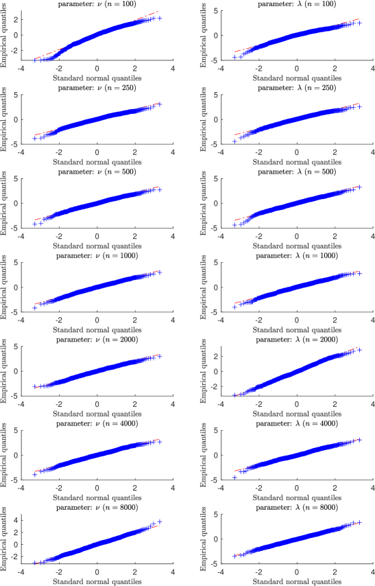
Figure S3: QQ plot of $\{z_{i,m}\}_{m=1}^{M}$ of Equation (S6.1) for the Poisson-Exp DGP.

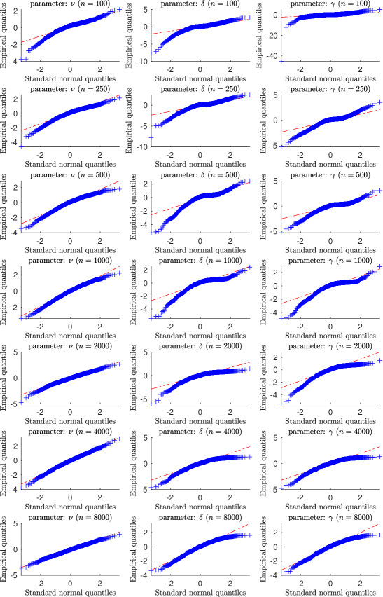
Figure S4: QQ plot of $\{z_{i,m}\}_{m=1}^{M}$ of Equation (S6.1) for the Poisson-IG DGP.

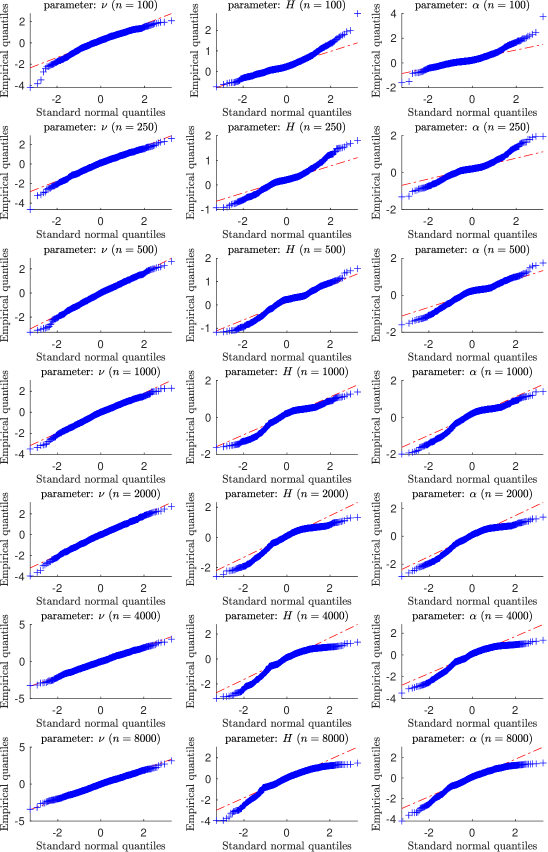
Figure S5: QQ plot of $\{z_{i,m}\}_{m=1}^{M}$ of Equation (S6.1) for the Poisson-Gamma DGP.

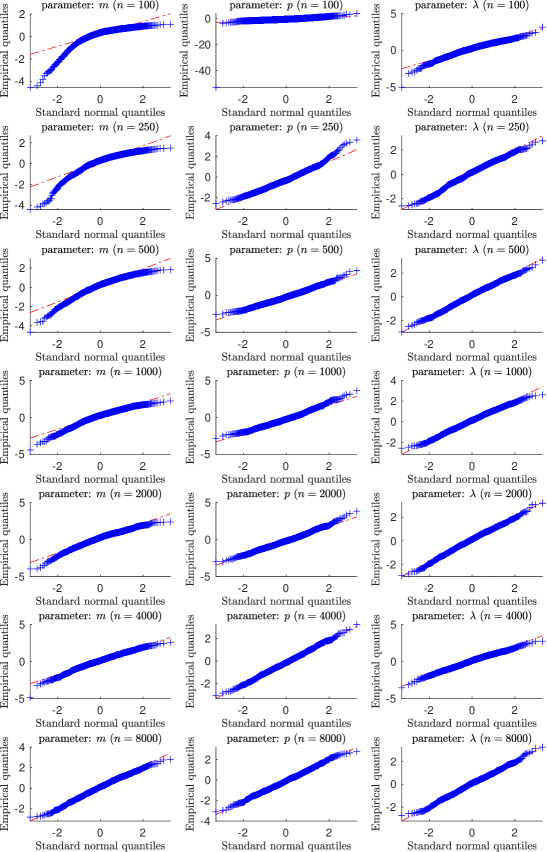
Figure S6: QQ plot of $\{z_{i,m}\}_{m=1}^{M}$ of Equation (S6.1) for the NB-Exp DGP.

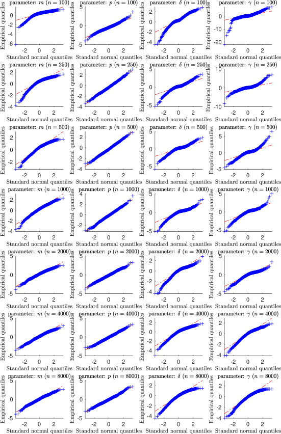
Figure S7: QQ plot of $\{z_{i,m}\}_{m=1}^{M}$ of Equation (S6.1) for the NB-IG DGP.

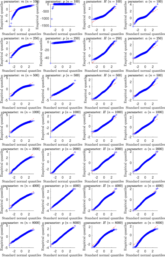
Figure S8: QQ plot of $\{z_{i,m}\}_{m=1}^{M}$ of Equation (S6.1) for the NB-Gamma DGP.

S6.4 Finite sample properties of the model selection procedure

This section illustrates the use, and finite sample properties, of the model selection procedure introduced in Section 3.1.3 of the main paper. Consider $n=4000$ equidistant observations of an IVT process on a grid of $\Delta=0.10$, i.e. $X_{\Delta},X_{2\Delta},\ldots,X_{n\Delta}$. For each of the six possible models, we then calculate the three goodness-of-fit measures, namely the value of the maximized composite likelihood function $CL$, the AIC-like composite likelihood information criteria $CLAIC$, and the BIC-like composite likelihood information criteria $CLBIC$. The model which has the maximum value of a criterion is “selected” by that criterion. We repeat this process for $100$ Monte Carlo replications and the six different DGPs using the parameters of Table S1. Figure S9 reports the “selection rates” of the models, i.e. the fraction of times that a model, given on the $x$-axis, is selected, for each of the three different criteria. Each panel in the figure corresponds to a particular DGP, as shown above, the respective panels.

Consider, for instance, the case where the true DGP is the NB-Exp IVT model. The results from using this DGP are given in the upper right panel of Figure S9. In this case, when we estimate the six different models and calculate the three goodness-of-fit measures, the true model (i.e. NB-Exp) has the highest composite likelihood value in $70\%$ of simulations. In contrast, the CLAIC and CLBIC result in selecting the true model in $73\%$ and $81\%$ of the simulations, respectively. Note that since the models considered here are not nested, it is not necessarily the case that the maximized composite likelihood value CL will be larger for the more complicated models.

Overall, Figure S9 indicates that the model selection procedure is quite accurate when the marginal distribution of the DGP is the Negative Binomial distribution. Conversely, when the marginal distribution of the DGP is the Poisson distribution, the correct model is chosen less often. However, in these situations, it is often the case that although the Negative Binomial distribution is (incorrectly) preferred to the Poisson distribution, the correct trawl function (autocorrelation structure) is nonetheless selected.

Lastly, to examine the effect of the tuning parameter $K$ on the model selection procedure, we ran the same experiment but using both $K=5$ and $K=20$ (results not shown here, but available upon request). We find that the model selection procedure deteriorates when $K=5$, while it performs similarly to that shown in Figure S9 when $K=20$, indicating that it is important to set $K$ sufficiently large value so that the selection criteria can properly distinguish between the models.

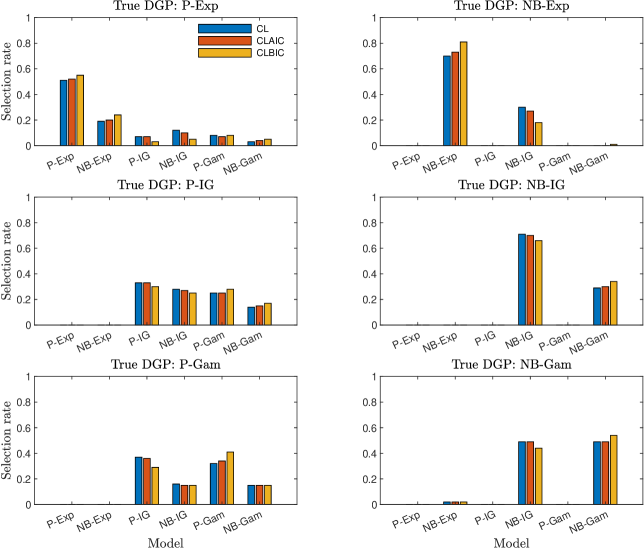
Figure S9: Simulation study of model selection procedure. Each plot represents the outcome of a separate Monte Carlo study, where the true DGP in the study is given above the plot. The numbers plotted are the average selection rates of the models given on the $x$-axis, using a given criterion over $M=100$ Monte Carlo simulations. For each Monte Carlo replication, $n=4000$ observations of the true DGP are simulated on a grid with step size $\Delta=0.10$. The parameters used in the study are given in Table S1 and we set $K=10$.

S6.5 Alternative simulation setup

We perform simulation experiments similar to those in the main paper but with a different set of simulation settings. The parameter values used for the DGPs in this study are given in Table S8; the associated implied marginal distributions of the underlying Lévy bases and autocorrelations of the IVT processes are shown in Figure S10.

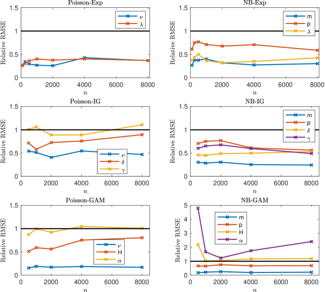
Figure S11: Root median square error (RMSE) of the MCL estimator divided by the RMSE of the GMM estimator. The underlying IVT process $X_{t}$ is simulated on the grid $t=\Delta,2\Delta,\ldots,n\Delta$, with $\Delta=0.10$, see Table S8 for the values of the parameters used in the simulations. For the Poisson-Exp and NB-Exp we set $K=1$; for the other DGPs we set $K=3$. We also conducted the comparison with $K=5$, as suggested in Barndorff-Nielsen et al. (2014) with similar results (results not presented here but available from the authors upon request).

In this simulation study, we simulate $n$ observations of an IVT process $X_{t}$ on an equidistant grid of size $\Delta=0.10$. For the IVTs based on the exponential trawl function, we set $K=1$, while we set $K=3$ for the remaining IVTs. This should be contrasted to the setup of the main paper, where we set $K=10$. The finite sample estimation results can be found in Tables S9–S14. Figure S11 plots the relative RMSE of the MCL estimator compared to the MM estimator; numbers smaller than one favour the MCL estimator.

Table S8: Parameter values used in simulation setup 2

DGP	$\nu$	$m$	$p$	$\lambda$	$\delta$	$\gamma$	$H$	$\alpha$
P-Exp	$5.00$			$1.00$
P-IG	$5.00$				$0.75$	$0.50$
P-Gamma	$5.00$						$0.50$	$0.75$
NB-Exp		$2.14$	$0.70$	$1.00$
NB-IG		$2.14$	$0.70$		$0.75$	$0.50$
NB-Gamma		$2.14$	$0.70$				$0.50$	$0.75$

Parameter values for the six different DGPs used in the simulation studies of the Supplementary Material. See the various Examples of the main paper for details. The value $m=\nu(1-p)/p$ with $\nu=5$ is chosen such that the first moment of the Poisson and Negative Binomial Lévy bases are matched. Marginal distributions and autocorrelation function implied by these parameter values are shown in Figure S10.

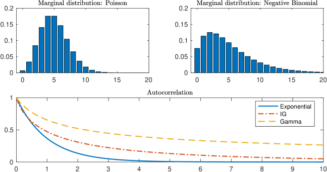
Figure S10: Marginal distributions of the Lévy bases and autocorrelations of the DGPs used in the simulation studies of Section S6.5. The marginal distribution and autocorrelation structure of IVT processes can be specified independently, resulting in six different DGPs in this setup (P-Exp, P-IG, P-Gamma, NB-Exp, NB-IG, NB-Gamma). The parameter values used to produce the plots are given in Table S8. Note that the marginal distribution shown in the top plots is of the underlying Lévy bases and not of the IVT process itself.

Table S9: CL estimation results: Poisson trawl process with exponential trawl function

	$\hat{\nu}$ ($\nu=5$)			$\hat{\lambda}$ ($\lambda=1$)
Nobs	Avg	Bias	RMSE	Avg	Bias	RMSE
$100$	$4.9994$	$-0.0006$	$0.6464$	$1.0131$	$0.0131$	$0.1220$
$250$	$5.0345$	$0.0345$	$0.4055$	$1.0099$	$0.0099$	$0.0756$
$500$	$5.0468$	$0.0468$	$0.2908$	$1.0074$	$0.0074$	$0.0623$
$1000$	$5.0100$	$0.0100$	$0.2181$	$1.0067$	$0.0067$	$0.0441$
$2000$	$5.0217$	$0.0217$	$0.1383$	$1.0026$	$0.0026$	$0.0288$
$4000$	$5.0103$	$0.0103$	$0.1058$	$1.0009$	$0.0009$	$0.0203$
$8000$	$5.0012$	$0.0012$	$0.0722$	$1.0005$	$0.0005$	$0.0150$

Median (Med.), median bias (Bias) and root median squared error (RMSE) of the MCL estimator. DGP: Poisson-Exponential IVT process. The IVT process $X_{t}$ is simulated on the grid $t=\Delta,2\Delta,\ldots,n\Delta$, with $\Delta=0.10$, see Table S8 for the values of the parameters used in the simulations. $K=1$. Number of Monte Carlo simulations: $500$.

Table S10: CL estimation results: Poisson trawl process with IG trawl function

	$\hat{\nu}$ ($\nu=5$)			$\hat{\delta}$ ($\delta=0.75$)			$\hat{\gamma}$ ($\gamma=0.5$)
Nobs	Avg	Bias	RMSE	Avg	Bias	RMSE	Avg	Bias	RMSE
$250$	$4.8852$	$-0.1148$	$0.6536$	$0.8535$	$0.1035$	$0.2654$	$5.6836$	$5.1836$	$31.0800$
$500$	$4.8907$	$-0.1093$	$0.4725$	$0.8241$	$0.0741$	$0.1833$	$1.1475$	$0.6475$	$6.2198$
$1000$	$4.9770$	$-0.0230$	$0.3128$	$0.7849$	$0.0349$	$0.1266$	$0.5699$	$0.0699$	$0.2729$
$2000$	$4.9789$	$-0.0211$	$0.2322$	$0.7641$	$0.0141$	$0.0890$	$0.5281$	$0.0281$	$0.1196$
$4000$	$4.9921$	$-0.0079$	$0.1516$	$0.7525$	$0.0025$	$0.0640$	$0.5118$	$0.0118$	$0.0773$
$8000$	$4.9997$	$-0.0003$	$0.1203$	$0.7533$	$0.0033$	$0.0421$	$0.5042$	$0.0042$	$0.0543$

Median (Med.), median bias (Bias) and root median squared error (RMSE) of the MCL estimator. DGP: Poisson-IG IVT. The IVT process $X_{t}$ is simulated on the grid $t=\Delta,2\Delta,\ldots,n\Delta$, with $\Delta=0.10$, see Table S8 for the values of the parameters used in the simulations. $K=3$. Number of Monte Carlo simulations: $500$.

Table S11: CL estimation results: Poisson trawl process with $\Gamma$ trawl function

	$\hat{\nu}$ ($\nu=5$)			$\hat{H}$ ($H=0.5$)			$\hat{\alpha}$ ($\alpha=0.75$)
Nobs	Avg	Bias	RMSE	Avg	Bias	RMSE	Avg	Bias	RMSE
$250$	$5.0958$	$0.0958$	$0.4897$	$0.6691$	$0.1691$	$0.3452$	$0.9620$	$0.2120$	$0.5434$
$500$	$4.9864$	$-0.0136$	$0.3323$	$0.6360$	$0.1360$	$0.2879$	$0.9710$	$0.2210$	$0.4283$
$1000$	$4.9781$	$-0.0219$	$0.2526$	$0.5957$	$0.0957$	$0.2109$	$0.8667$	$0.1167$	$0.3183$
$2000$	$4.9866$	$-0.0134$	$0.1776$	$0.5765$	$0.0765$	$0.1531$	$0.8480$	$0.0980$	$0.2443$
$4000$	$4.9789$	$-0.0211$	$0.1233$	$0.5519$	$0.0519$	$0.1156$	$0.8223$	$0.0723$	$0.1678$
$8000$	$4.9720$	$-0.0280$	$0.0945$	$0.5515$	$0.0515$	$0.0864$	$0.8147$	$0.0647$	$0.1234$

Median (Med.), median bias (Bias) and root median squared error (RMSE) of the MCL estimator. DGP: Poisson-Gamma IVT. The IVT process $X_{t}$ is simulated on the grid $t=\Delta,2\Delta,\ldots,n\Delta$, with $\Delta=0.10$, see Table S8 for the values of the parameters used in the simulations. $K=3$. Number of Monte Carlo simulations: $500$.

Table S12: CL estimation results: NB trawl process with exponential trawl function

	$\hat{m}$ ($m=2.1429$)			$\hat{p}$ ($p=0.7$)			$\hat{\lambda}$ ($\lambda=1$)
Nobs	Avg	Bias	RMSE	Avg	Bias	RMSE	Avg	Bias	RMSE
$100$	$2.7614$	$0.6186$	$0.8445$	$0.6268$	$-0.0732$	$0.1010$	$1.0021$	$0.0021$	$0.1902$
$250$	$2.3957$	$0.2528$	$0.4848$	$0.6692$	$-0.0308$	$0.0618$	$0.9921$	$-0.0079$	$0.1206$
$500$	$2.1957$	$0.0529$	$0.3009$	$0.6883$	$-0.0117$	$0.0394$	$1.0038$	$0.0038$	$0.0791$
$1000$	$2.2200$	$0.0771$	$0.2357$	$0.6912$	$-0.0088$	$0.0309$	$1.0008$	$0.0008$	$0.0596$
$2000$	$2.1887$	$0.0458$	$0.1632$	$0.6935$	$-0.0065$	$0.0215$	$1.0030$	$0.0030$	$0.0410$
$4000$	$2.1630$	$0.0201$	$0.1126$	$0.6967$	$-0.0033$	$0.0144$	$0.9999$	$-0.0001$	$0.0273$
$8000$	$2.1557$	$0.0128$	$0.0805$	$0.6985$	$-0.0015$	$0.0109$	$1.0012$	$0.0012$	$0.0210$

Median (Med.), median bias (Bias) and root median squared error (RMSE) of the MCL estimator. DGP: Negative Binomial-Exponential IVT process. The IVT process $X_{t}$ is simulated on the grid $t=\Delta,2\Delta,\ldots,n\Delta$, with $\Delta=0.10$, see Table S8 for the values of the parameters used in the simulations. $K=1$. Number of Monte Carlo simulations: $500$.

Table S13: CL estimation results: NB trawl process with IG trawl function

	$\hat{m}$ ($m=2.1429$)			$\hat{p}$ ($p=0.7$)			$\hat{\delta}$ ($\delta=0.75$)			$\hat{\gamma}$ ($\gamma=0.5$)
Nobs	Avg	Bias	RMSE	Avg	Bias	RMSE	Avg	Bias	RMSE	Avg	Bias	RMSE
$250$	$2.5049$	$0.3621$	$0.5605$	$0.6361$	$-0.0639$	$0.0827$	$0.9671$	$0.2171$	$0.3323$	$0.6664$	$0.1664$	$0.2521$
$500$	$2.3485$	$0.2056$	$0.4236$	$0.6688$	$-0.0312$	$0.0632$	$0.8739$	$0.1239$	$0.2095$	$0.5738$	$0.0738$	$0.1402$
$1000$	$2.2625$	$0.1197$	$0.3055$	$0.6767$	$-0.0233$	$0.0450$	$0.7991$	$0.0491$	$0.1460$	$0.5280$	$0.0280$	$0.0986$
$2000$	$2.1975$	$0.0547$	$0.2073$	$0.6937$	$-0.0063$	$0.0303$	$0.7757$	$0.0257$	$0.1099$	$0.5147$	$0.0147$	$0.0769$
$4000$	$2.1757$	$0.0328$	$0.1384$	$0.6936$	$-0.0064$	$0.0199$	$0.7777$	$0.0277$	$0.0800$	$0.5203$	$0.0203$	$0.0573$
$8000$	$2.1661$	$0.0232$	$0.0970$	$0.6978$	$-0.0022$	$0.0152$	$0.7631$	$0.0131$	$0.0560$	$0.5127$	$0.0127$	$0.0380$

Median (Med.), median bias (Bias) and root median squared error (RMSE) of the MCL estimator. DGP: Negative Binomial-IG IVT. The IVT process $X_{t}$ is simulated on the grid $t=\Delta,2\Delta,\ldots,n\Delta$, with $\Delta=0.10$, see Table S8 for the values of the parameters used in the simulations. $K=3$. Number of Monte Carlo simulations: $500$.

Table S14: CL estimation results: NB trawl process with $\Gamma$ trawl function

	$\hat{m}$ ($m=2.1429$)			$\hat{p}$ ($p=0.7$)			$\hat{H}$ ($H=0.5$)			$\hat{\alpha}$ ($\alpha=0.75$)
Nobs	Avg	Bias	RMSE	Avg	Bias	RMSE	Avg	Bias	RMSE	Avg	Bias	RMSE
$500$	$2.6635$	$0.5206$	$0.5684$	$0.6240$	$-0.0760$	$0.0873$	$3.0978$	$2.5978$	$2.5978$	$4.6910$	$3.9410$	$3.9414$
$1000$	$2.4640$	$0.3212$	$0.4184$	$0.6510$	$-0.0490$	$0.0608$	$1.1213$	$0.6213$	$0.6213$	$1.6475$	$0.8975$	$0.8975$
$2000$	$2.3565$	$0.2136$	$0.3091$	$0.6659$	$-0.0341$	$0.0461$	$0.7854$	$0.2854$	$0.2887$	$1.1460$	$0.3960$	$0.4207$
$4000$	$2.2840$	$0.1411$	$0.1944$	$0.6739$	$-0.0261$	$0.0327$	$0.7204$	$0.2204$	$0.2391$	$1.0852$	$0.3352$	$0.3518$
$8000$	$2.2302$	$0.0873$	$0.1583$	$0.6843$	$-0.0157$	$0.0256$	$0.7034$	$0.2034$	$0.2142$	$1.0659$	$0.3159$	$0.3259$

Median (Med.), median bias (Bias) and root median squared error (RMSE) of the MCL estimator. DGP: Negative Binomial-Gamma IVT process. The IVT process $X_{t}$ is simulated on the grid $t=\Delta,2\Delta,\ldots,n\Delta$, with $\Delta=0.10$, see Table S8 for the values of the parameters used in the simulations. $K=3$. Number of Monte Carlo simulations: $500$.

Appendix S7 Empirical study

This section contains additional details on the data pre-processing used in the empirical study, see Subsection S7.1, and additional forecasting results, see Subsection S7.2.

S7.1 Details for the empirical study

We will now provide some additional details on the data preprocessing carried out for the empirical study. In the article, we analyse the time series of the bid-ask spread, measured in U.S. dollar cents, of the Agilent Technologies Inc. stock (ticker: A) on a single day, May $4$, $2020$. The A stock is traded on the New York Stock Exchange, which is open from $9$:$30$ AM to $4$ PM. To avoid opening effects, we consider the data from $10$:$30$ AM to $4$ PM, i.e. we discard the first $60$ minutes of the day. Our data is gathered from the Trade and Quote database and cleaned using the approach proposed in Barndorff-Nielsen et al. (2009). The data is available at a very high frequency but to obtain equidistant data, we sample the observations with $\Delta=\frac{1}{12}$ minutes (i.e. $5$ seconds) time steps, using the previous tick approach, starting at $10$:$30$ AM, resulting in $n=3961$ observations.

S7.2 Additional forecasting results

Figures S12a–S12c report forecasting results analogous to those of Section 6.1 in the main paper, but now using the conditional mode, instead of the conditional mean, as a point forecast. That is, using the notation of Section 6.1 in the main paper, we set $\hat{x}_{i|i-h}=\arg\max_{k}\widehat{\mathbb{P}}(X_{i|i-h}=k)$, where $\widehat{\mathbb{P}}$ is the estimated predictive PMF of the IVT model.

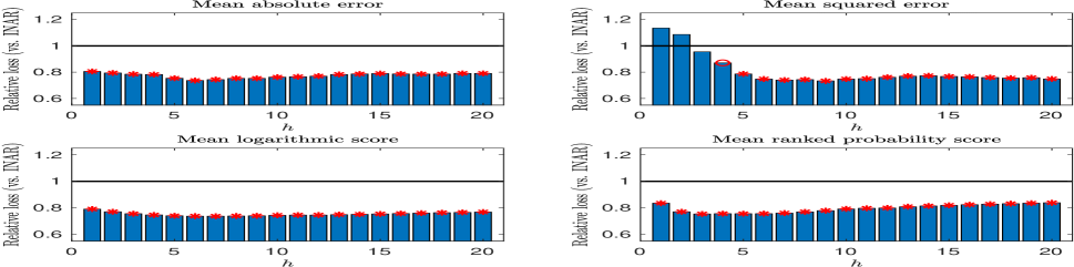
(a) NB-Gamma versus Poissonian INAR(1)

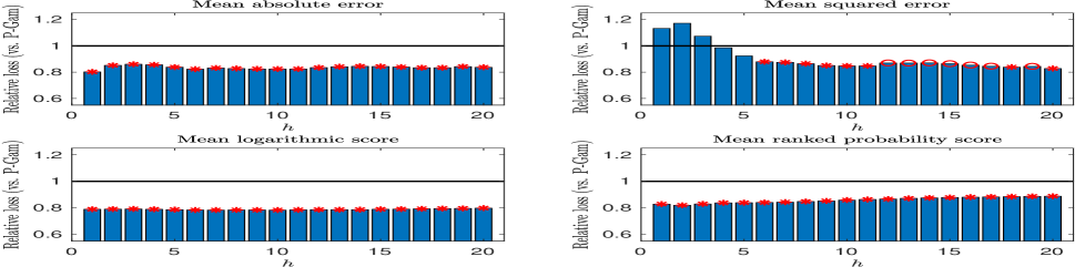
(b) NB-Gamma versus Poisson-Gamma model

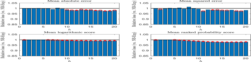
(c) NB-Gamma versus NB-Exponential

Figure S12: Forecasting the spread level of the A stock on May 4, 2020. Four different loss metrics and twenty forecast horizons, $h=1,2,\ldots,20$. The numbers plotted are relative average losses of the NB-Gamma forecasting model, compared with the (a) Poissonian INAR(1) model, the (b) Poisson-Gamma model, and the (c) NB-Exponential, over $n_{oos}=720$ out-of-sample forecasts. A circle above the bars indicates rejection null of equal forecasting performance between the two models, against the alternative that the NB-Gamma model provides superior forecasts, using the Diebold-Mariano (Diebold and Mariano 1995) test at a $5\%$ level; an asterisk denotes rejection at a $1\%$ level.

Appendix S8 Details concerning integer-valued Lévy bases

S8.1 Poisson Lévy basis

Consider the case where the Lévy basis is Poisson, i.e. $L^{\prime}\sim\textnormal{Poi}(\nu)$ for some intensity $\nu>0.$ For a bounded Borel set $B$ with $Leb(B)<\infty,$ we have

$$L(B)\sim\textnormal{Poi}(\nu Leb(B)).$$

The cumulants, in this case, are $\kappa_{j}=\nu$ for all $j\geq 0$.

S8.2 Negative binomial Lévy basis

We follow Barndorff-Nielsen et al. (2012, 2014) and denote by $NB(m,p)$ the negative binomial law with parameters $m\in\mathbb{N}$ and $p\in(0,1).$ Recall, that a negative binomial random variable is positively valued and can be interpreted as the number of successes, $k,$ until $m$ failures in a sequence of iid Bernoulli trials, each with the probability of success $p.$ Let $L^{\prime}\sim NB(m,p);$ it holds that

$$P(L^{\prime}=k)=\frac{\Gamma(m+k)}{k!\Gamma(m)}(1-p)^{m}p^{k},\quad k=0,1,2,\ldots.$$

As is well known, we have that $L^{\prime}_{t}\sim NB(mt,p)$ and therefore, for a Borel set $B$, it holds that $L(B)\sim NB(Leb(B)m,p)$, which implies

$$P(L(B)=k)=\frac{\Gamma(Leb(B)m+k)}{k!\Gamma(Leb(B)m)}(1-p)^{Leb(B)m}p^{k},\quad k=0,1,2,\ldots.$$

Here the relevant cumulants are $\kappa_{1}=\frac{pm}{1-p}$, $\kappa_{2}=\frac{pm}{(1-p)^{2}}$ and $\kappa_{4}=m\frac{p+4p^{2}+p^{3}}{(1-p)^{4}}$.

S8.3 Skellam Lévy basis

The Skellam distribution is the distribution of the difference of two Poisson processes $N_{t}^{+}$ and $N_{t}^{-}$ and is therefore integer-valued. Let $N_{t}^{\pm}\sim\textnormal{Poi}(\psi^{\pm})$ with $\psi^{\pm}>0$; then $S:=N_{t}^{+}-N_{t}^{-}\sim\textnormal{Skellam}(\psi^{+},\psi^{-}).$ Further, the Skellam Lévy process $(L_{t}^{\prime})_{t\geq 0}$ with $L_{1}^{\prime}\sim\textnormal{Skellam}(\psi^{+},\psi^{-})$ has the marginal distribution $L_{t}^{\prime}\sim\textnormal{Skellam}(t\psi^{+},t\psi^{-})$ (Barndorff-Nielsen et al. 2012), meaning that for a Borel set $B,$ we have $L(B)\sim\textnormal{Skellam}(Leb(B)\psi^{+},Leb(B)\psi^{-}).$ The PMF of the random variable $X\sim\textnormal{Skellam}(\psi^{+},\psi^{-})$ is given by

$$g(k;\psi^{+},\psi^{-}):=P(X=k)=e^{-(\psi^{+}+\psi^{-})}\left(\frac{\psi^{+}}{\psi^{-}}\right)^{k/2}I_{k}\left(2\sqrt{\psi^{+}\psi^{-}}\right),$$

where $I_{\nu}(x)$ is the modified Bessel function of the first kind (see e.g. Abramowitz and Stegun (1972)) with parameter $\nu$ evaluated at $x.$ In the symmetric case, $\psi^{+}=\psi^{-}=\psi,$ this reduces to $g(k;\psi):=e^{-2\psi}I_{k}(2\psi)$. The cumulants are easily seen to be $\kappa_{j}=\psi^{+}-\psi^{-}$ for $j$ odd and $\kappa_{j}=\psi^{+}+\psi^{-}$ for $j$ even.

S8.4 $\Delta NB$ Lévy basis

Analogous to the Skellam process, we can consider the difference of two Lévy seeds which have negative binomials as their laws; Barndorff-Nielsen et al. (2012) call this a $\Delta NB$ Lévy process. Let $L^{\pm}\sim NB(m^{\pm},p^{\pm})$ be independent Lévy seeds with negative binomial laws. Barndorff-Nielsen et al. (2012) show that for $k\geq 0,$ the difference Lévy seed $L^{\prime}=L^{+}-L^{-}$ has PMF

$$P(L^{\prime}=k)=(1-p^{+})^{m^{+}}(1-p^{-})^{m^{-}}\frac{(p^{+})^{k}(m^{+})_{k}}{k!}F(m^{+}+k,m^{-};k+1;p^{+}p^{-}),$$ (S8.1)

where

$$F(\alpha,\beta;\gamma;z)=\sum_{n=0}^{\infty}\frac{(\alpha)_{n}(\beta)_{n}}{(\gamma)_{n}}\frac{z^{n}}{n!},\quad z\in[0,1),\quad\alpha,\beta,\gamma>0,$$

is the hypergeometric function, see e.g. Abramowitz and Stegun (1972), and $(\alpha)_{n}=\frac{\Gamma(\alpha+n)}{\Gamma(\alpha)}$ is the Pochhammer symbol. The PMF for $k\leq 0$ is, by symmetry, given as S8.1, mutatis mutandis. The resulting distribution is denoted as $L^{\prime}\sim\Delta NB(m^{+},p^{+},m^{-},p^{-})$ and it is easy to show that (Barndorff-Nielsen et al. 2012) the Lévy process corresponding to $L^{\prime}$ has marginal distribution $L_{t}^{\prime}\sim\Delta NB(tm^{+},p^{+},tm^{-},p^{-}),$ meaning that we have for a Borel set $B$,

$$L(B)\sim NB(Leb(B)m^{+},p^{+},Leb(B)m^{-},p^{-}).$$

The cumulants for the $\Delta NB$ Lévy seed are easily deduced from those of the negative binomial ones, recalling that the $\Delta NB$ law is the difference of two independent NB random variables.

Appendix S9 Details concerning parametric trawl functions

The expressions for the likelihoods in the previous section reveal that we are interested in calculating expressions such as $Leb(A_{t}\backslash A)$ and $Leb(A_{t}\cap A)$ for different trawl functions. In this section we derive the required results for various trawls based on the superposition trawl function $d(s)=\int_{0}^{\infty}e^{\lambda s}\pi(d\lambda)$, $s\leq 0$, see also the main paper.

S9.1 The exponential trawl

The case where the measure $\pi$ has an atom at $\lambda>0,$ i.e. $\pi(dx)=\delta_{\lambda}(dx),$ where $\delta_{y}(\cdot)$ is the Dirac delta function at $y\in\mathbb{R}_{+},$ we get $d(s)=e^{\lambda s}.$ Consequently, for $t\geq 0,$

$$Leb(A)=\lambda^{-1},\quad Leb(A_{t}\backslash A)=\lambda^{-1}(1-e^{-\lambda t}),\quad Leb(A_{t}\cap A)=\lambda^{-1}e^{-\lambda t}.$$

This implies the correlation function

$$\rho(h)=\exp(-\lambda h),\quad h>0.$$

S9.2 The finite superposition exponential trawl

Let $\pi$ have finitely many atoms, i.e. $\pi(dx)=\sum_{i=1}^{q}w_{i}\delta_{\lambda_{i}}(dx)$ for $q\in\mathbb{N}.$ Then

$$d(s)=\sum_{i=1}^{q}w_{i}e^{\lambda_{i}s},$$

and

$$Leb(A)=\sum_{i=1}^{q}w_{i}\lambda_{i}^{-1},\quad Leb(A_{t}\backslash A)=\sum_{i=1}^{q}w_{i}\lambda_{i}^{-1}(1-e^{-\lambda_{i}t}),\quad Leb(A_{t}\cap A)=\sum_{i=1}^{q}w_{i}\lambda_{i}^{-1}e^{-\lambda_{i}t}.$$

This implies the correlation function

$$\rho(h)=\left(\sum_{i=1}^{q}\omega_{i}\lambda_{i}^{-1}\right)^{-1}\sum_{i=1}^{q}\omega_{i}\lambda_{i}^{-1}\exp(-\lambda_{i}h),\quad h>0.$$

S9.3 The GIG trawl

A flexible class of trawl functions can be specified through the generalized inverse Gaussian (GIG) density function (see e.g. Barndorff-Nielsen et al. (2014)),

$$f_{\pi}(x)=\frac{(\gamma/\delta)^{\nu}}{2K_{\nu}(\delta\gamma)}x^{\nu-1}\exp\left(-\frac{1}{2}(\delta^{2}x^{-1}+\gamma^{2}x)\right),$$

where $\nu\in\mathbb{R}$ and $\gamma,\delta\geq 0$ with both not equal to zero simultaneously. $K_{\nu}(x)$ is the modified Bessel function of the third kind with parameter $\nu,$ evaluated at $x$ (e.g. Abramowitz and Stegun (1972)). Suppose now, that $\pi$ has density $f_{\pi},$ i.e. $\pi(d\lambda)=f_{\pi}(\lambda)d\lambda.$ For $s\leq 0,$ the trawl function becomes

$$d(s)=\int_{0}^{\infty}e^{\lambda s}f_{\pi}(\lambda)d\lambda=\left(1-\frac{2s}{\gamma^{2}}\right)^{-\nu/2}\frac{K_{\nu}\left(\delta\gamma\alpha_{s}\right)}{K_{\nu}(\delta\gamma)},$$

whereas

$$Leb(A)=\frac{\gamma}{\delta}\frac{K_{\nu-1}(\delta\gamma)}{K_{\nu}(\delta\gamma)},\quad Leb(A_{t}\cap A)=\frac{\gamma\alpha_{t}^{-\nu+1}}{\delta}\frac{K_{\nu-1}(\delta\gamma\alpha_{t})}{K_{\nu}(\delta\gamma)},$$

and

$$Leb(A_{t}\backslash A)=\frac{\gamma}{\delta K_{\nu}(\delta\gamma)}\left(K_{\nu-1}(\delta\gamma)-\alpha_{t}^{-\nu+1}K_{\nu-1}(\delta\gamma\alpha_{t})\right),$$

where $\alpha_{t}:=\sqrt{\frac{2t}{\gamma^{2}}+1}.$ This implies the correlation function

$$\rho(h)=\alpha_{h}^{-\nu+1}\frac{K_{\nu-1}(\delta\gamma\alpha_{h})}{K_{\nu-1}(\delta\gamma)},\quad h>0.$$

S9.4 The IG trawl

The inverse Gaussian distribution is a special case of the GIG distributions, where $\nu=\frac{1}{2}.$ In this case, the trawl function simplifies to

$$d(s)=\left(1-\frac{2s}{\gamma^{2}}\right)^{-1/2}\exp\left(\delta\gamma\left(1-\sqrt{1-\frac{2s}{\gamma^{2}}}\right)\right),\quad s\leq 0,$$

which means that

$$Leb(A)=\frac{\gamma}{\delta},\quad Leb(A_{t}\cap A)=\frac{\gamma}{\delta}e^{\delta\gamma(1-\alpha_{t})},\quad Leb(A_{t}\backslash A)=\frac{\gamma}{\delta}\left(1-e^{\delta\gamma(1-\alpha_{t})}\right),$$

where again $\alpha_{t}=\sqrt{\frac{2t}{\gamma^{2}}+1}.$ This implies the correlation function

$$\rho(h)=\exp(\delta\gamma(1-\alpha_{h})),\quad h>0.$$

S9.5 The $\Gamma$ trawl

An interesting case, capable of generating long memory in the trawl process, is given by the $\Gamma$ trawl. Suppose that $\pi$ has the $\Gamma(1+H,\alpha)$ density,

$$f_{\pi}(\lambda)=\frac{1}{\Gamma(1+H)}\alpha^{1+H}\lambda^{H}e^{-\lambda\alpha},$$

where $\alpha>0$ and $H>0.$ Now,

$$d(s)=\left(1-\frac{s}{\alpha}\right)^{-(H+1)},\quad s\leq 0,$$

which implies

$$Leb(A)=\frac{\alpha}{H},\quad Leb(A_{t}\cap A)=\frac{\alpha}{H}\left(1+\frac{t}{\alpha}\right)^{-H},\quad Leb(A_{t}\backslash A)=\frac{\alpha}{H}\left(1-\left(1+\frac{t}{\alpha}\right)^{-H}\right).$$

This yields the correlation function

$$\rho(h)=Corr(L(A_{t+h}),L(A_{t}))=\frac{Leb(A_{h}\cap A)}{Leb(A)}=\left(1+\frac{h}{\alpha}\right)^{-H},$$

so that

$$\int_{0}^{\infty}\rho(h)dh=\left\{\begin{array}[]{lr}\infty&\textnormal{if}\quad H\in(0,1],\\ \frac{\alpha}{H-1}&\textnormal{if}\quad H>1,\end{array}\right.$$

from which we see, that the trawl process has long memory for $H\in(0,1].$

Appendix S10 Details concerning gradients

Recall that we have the composite log-likelihood function

$$l_{CL}(\theta;x):=l_{CL}^{(K)}(\theta;x)=\log L_{CL}^{(K)}(\theta;x)=\sum_{k=1}^{K}\sum_{i=1}^{n-k}\log f(x_{i+k},x_{i};\theta).$$

Let $\theta_{i}$ be an element of $\theta$. The derivative of $l_{CL}(\theta;x)$ wrt. $\theta_{i}$ is

$$\frac{\partial}{\partial\theta_{i}}l_{CL}(\theta;x)=\frac{\partial}{\partial\theta_{i}}\log L_{CL}^{(K)}(\theta;x)=\sum_{k=1}^{K}\sum_{i=1}^{n-k}\frac{1}{f(x_{i+k},x_{i};\theta)}\frac{\partial}{\partial\theta_{i}}f(x_{i+k},x_{i};\theta).$$ (S10.1)

Recall also that

$$f(x_{i+k},x_{i};\theta) =\sum_{c=-\infty}^{\infty}P_{1,i,k}^{(c)}\cdot P_{2,i,k}^{(c)}\cdot P_{3,k}^{(c)}$$

with

$$P_{1,i,k}^{(c)}:=\mathbb{P}\left(L(A_{k\Delta}\setminus A)=x_{i+k}-c\right),\quad P_{2,i,k}^{(c)}=\mathbb{P}\left(L(A_{k\Delta}\setminus A)=x_{i}-c\right),\quad P_{3,k}^{(c)}=\mathbb{P}\left(L(A_{k\Delta}\cap A)=c\right),$$

implying that

$$\frac{\partial}{\partial\theta_{i}}f(x_{i+k},x_{i};\theta) =\sum_{c=-\infty}^{\infty}\left(\frac{\partial}{\partial\theta_{i}}P_{1,i,k}^{(c)}\cdot P_{2,i,k}^{(c)}\cdot P_{3,k}^{(c)}+P_{1,i,k}^{(c)}\cdot\frac{\partial}{\partial\theta_{i}}P_{2,i,k}^{(c)}\cdot P_{3,k}^{(c)}+P_{1,i,k}^{(c)}\cdot P_{2,i,k}^{(c)}\cdot\frac{\partial}{\partial\theta_{i}}P_{3,k}^{(c)}\right).$$ (S10.2)

The terms $P_{1,i,k}^{(c)},P_{2,i,k}^{(c)},P_{3,k}^{(c)}$ are calculated in the numerical maximization of the composite likelihood routine for all $c$. The aim of this section is to calculate $\frac{\partial}{\partial\theta_{i}}P_{j,i,k}^{(c)}$ for $j=1,2,3$, so that the gradient of the log-likelihood function is easily calculated using Equations (S10.1) and (S10.2). It is clear that $\frac{\partial}{\partial\theta_{i}}P_{j,i,k}^{(c)}$ will depend on both the Lévy basis as well as the form of the trawl set (and hence the trawl function). We first supply the relevant derivations for the Poisson Lévy basis (Section S10.2) and the Negative Binomial Lévy basis (Section S10.3), and then the trawl functions Exp, SupExp, IG, and $\Gamma$ (Sections S10.4–S10.7).

S10.1 Some preliminary practical details

In our numerical implementation of the composite likelihood methods, we often have restrictions on some parameters. Most notably, we have positivity restriction, e.g. we require that the intensity $\nu>0$ for the Poisson Lévy basis. One could impose such restrictions by using a constrained optimization procedure when performing the numerical optimization of the log composite likelihood function $l_{CL}(\theta;x)$. We prefer to work with an unconstrained optimization procedure, by transforming the parameters such that they are fulfilling their restrictions automatically. That is if $\theta$ is a restricted parameter, we find an invertible transformation function $g$, such that $\tilde{\theta}=g^{-1}(\theta)\in\mathbb{R}$ is unrestricted. The unconstrained numerical optimizer is optimizing over the unrestricted parameter $\tilde{\theta}$ and arrives at, say, $\tilde{\theta}^{*}$. Our estimate of $\theta$ is thus $\hat{\theta}=g(\tilde{\theta}^{*})$. Consequently, it is necessary to correct for this when calculating standard errors (delta rule) as well as when supplying a gradient for our numerical optimization scheme. The reason is that the calculations concerning the gradient, detailed in the previous section, are with respect to $\theta$, and not $\tilde{\theta}$, which is the actual parameter being used in the numerical optimization procedure. In the case of a transformed variable, the gradient that should be supplied to the machine is therefore not the one given in (S10.2), but rather

$$\frac{\partial}{\partial\tilde{\theta}_{i}}f(x_{i+k},x_{i};\theta)=\frac{\partial}{\partial\theta_{i}}f(x_{i+k},x_{i};\theta)\frac{\partial\theta_{i}}{\partial\tilde{\theta}_{i}}=\frac{\partial}{\partial\theta_{i}}f(x_{i+k},x_{i};\theta)\frac{\partial}{\partial\tilde{\theta}_{i}}g(\tilde{\theta}).$$

In this paper two restrictions are encountered: many parameters are positive, while a few are restricted to be in the unit interval. If $\theta>0$ is a positive parameter, we use a log transformation by defining the new parameter $\tilde{\theta}$ through

$$\tilde{\theta}=g^{-1}(\theta)=\log\theta,\qquad\theta=g(\tilde{\theta})=\exp(\tilde{\theta}).$$

If $p\in(0,1)$ is a parameter, we use an inverse logistic (sigmoid) transformation,

$$\tilde{p}=g^{-1}(p)=\log\left(\frac{p}{1-p}\right),\qquad p=g(\tilde{p})=\frac{1}{1+\exp(-\tilde{p})}.$$

S10.2 Poisson Lévy basis

Let $L^{\prime}\sim Poi(\nu)$ and recall that for a Borel set $B$, this implies

$$\mathbb{P}\left(L(B)=x\right)=\frac{[\nu Leb(B)]^{x}\exp(-\nu Leb(B))}{x!}.$$

We deduce, that for a generic parameter $\theta\neq\nu$,

$$\frac{\partial}{\partial\theta}\mathbb{P}\left(L(B)=x\right)=\left(xLeb(B)^{-1}-\nu\right)\mathbb{P}\left(L(B)=x\right)\frac{\partial}{\partial\theta}Leb(B).$$

The only ingredient left to calculate is

$$\frac{\partial}{\partial\nu}\mathbb{P}\left(L(B)=x\right)=\left(x\nu^{-1}-Leb(B)\right)\mathbb{P}\left(L(B)=x\right).$$

S10.3 Negative Binomial Lévy basis

Recall that in the case where the Lévy seed $L^{\prime}$ is distributed as a Negative Binomial random variable with parameters $m>0$ and $p\in[0,1]$, we have $L(B)\sim NB(Leb(B)m,p)$, which implies

$$P(L(B)=x)=\frac{\Gamma(Leb(B)m+x)}{x!\Gamma(Leb(B)m)}(1-p)^{Leb(B)m}p^{x},\quad x=0,1,2,\ldots.$$

Using the well-known property of the $\Gamma$ function that $\Gamma(x+1)=x\Gamma(x)$ (Gradshteyn and Ryzhik 2007, p. 904), we can write

$$P(L(B)=x)=\left(Leb(B)m+x-1\right)\left(Leb(B)m+x-2\right)\cdots\left(Leb(B)m\right)\frac{1}{x!}(1-p)^{Leb(B)m}p^{x},$$

for $k=0,1,2,\ldots$. We deduce, that for a generic parameter $\theta\neq m,p$,

$$\frac{\partial}{\partial\theta} P(L(B)=x)$$

$$=\left(\frac{\partial}{\partial\theta}Leb(B)\right)mP(L(B)=x)\left(\log(1-p)+\frac{1}{Leb(B)m}+\frac{1}{Leb(B)m+1}+\cdots+\frac{1}{Leb(B)m+x-1}\right).$$

The only ingredients left to calculate are

$$\frac{\partial}{\partial p} P(L(B)=x)=P(L(B)=x)\left(\frac{x}{p}-\frac{Leb(B)m}{1-p}\right),$$

and

$$\frac{\partial}{\partial m}P(L(B)=x)$$

$$=P(L(B)=x)Leb(B)\left(\log(1-p)+\frac{1}{Leb(B)m}+\frac{1}{Leb(B)m+1}+\cdots+\frac{1}{Leb(B)m+x-1}\right).$$

S10.4 Exponential trawl function

Let $L^{\prime}$ be a generic Lévy seed and $d(s)=\exp(\lambda s)$ for $s\leq 0$. Recall that for $t>0$,

$$Leb(A_{t}\setminus A)=\lambda^{-1}(1-\exp(-\lambda t)),\qquad Leb(A_{t}\cap A)=\lambda^{-1}\exp(-\lambda t).$$

It is not difficult to show that

$$\frac{\partial}{\partial\lambda}Leb(A_{t}\setminus A)=\lambda^{-1}\left(t\exp(-\lambda t)-\lambda^{-1}(1-\exp(-\lambda t))\right),$$

while

$$\frac{\partial}{\partial\lambda}Leb(A_{t}\cap A)=-\lambda^{-1}\exp(-\lambda t)\left(\lambda^{-1}+t\right).$$

S10.5 SupExp trawl function

Let $L^{\prime}$ be a generic Lévy seed and $d(s)$ be the supExp trawl function (see above). Recall that for $t>0$,

$$Leb(A_{t}\setminus A)=\sum_{i=1}^{q}w_{i}\lambda_{i}^{-1}(1-e^{-\lambda_{i}t}),\qquad Leb(A_{t}\cap A)=\sum_{i=1}^{q}w_{i}\lambda_{i}^{-1}e^{-\lambda_{i}t}.$$

It is not difficult to show that for $j=1,2,\ldots,q,$

$$\frac{\partial}{\partial\lambda_{j}}Leb(A_{t}\setminus A) =w_{j}\lambda_{j}^{-1}\left(t\exp(-\lambda_{j}t)-\lambda_{j}^{-1}(1-\exp(-\lambda_{j}t))\right),$$

$$\frac{\partial}{\partial\lambda_{j}}Leb(A_{t}\cap A) =-w_{j}\lambda_{j}^{-1}\exp(-\lambda_{j}t)\left(\lambda_{j}^{-1}+t\right),$$

while

$$\frac{\partial}{\partial w_{j}}Leb(A_{t}\setminus A) =\lambda_{j}^{-1}(1-e^{-\lambda_{j}t}),$$

$$\frac{\partial}{\partial w_{j}}Leb(A_{t}\cap A) =\lambda_{j}^{-1}e^{-\lambda_{j}t}.$$

S10.6 IG trawl function

Let $L^{\prime}$ be a generic Lévy seed and $d(s)$ be the IG trawl (see above). Recall that, for $t>0$,

$$Leb(A_{t}\setminus A)=\frac{\gamma}{\delta}\left(1-\exp(\delta\gamma(1-\alpha_{t}))\right),\quad Leb(A_{t}\cap A)=\frac{\gamma}{\delta}\exp(\delta\gamma(1-\alpha_{t})),$$

where $\alpha_{t}=\sqrt{\frac{2t}{\gamma^{2}}+1}$.

We can show that

$$\frac{\partial}{\partial\delta}Leb(A_{t}\setminus A) =-\delta^{-1}Leb(A_{t}\setminus A)-\gamma^{2}\delta^{-1}(1-\alpha_{t})\exp(\delta\gamma(1-\alpha_{t})),$$

$$\frac{\partial}{\partial\gamma}Leb(A_{t}\setminus A) =-\gamma^{-1}Leb(A_{t}\setminus A)-\gamma\exp(\delta\gamma(1-\alpha_{t}))[1-\alpha_{t}+2\gamma^{-2}\alpha_{t}^{-1}t],$$

and

$$\frac{\partial}{\partial\delta}Leb(A_{t}\cap A) =Leb(A_{t}\cap A)(\gamma(1-\alpha_{t})-\delta^{-1}),$$

$$\frac{\partial}{\partial\gamma}Leb(A_{t}\cap A) =Leb(A_{t}\cap A)(\gamma^{-1}+\delta(1-\alpha_{t})+2\delta\gamma^{-2}\alpha_{t}^{-1}t).$$

S10.7 $\Gamma$ trawl function

Let $L^{\prime}$ be a generic Lévy seed and $d(s)$ be the $\Gamma$ trawl (see above). Recall that, for $t>0$,

$$Leb(A_{t}\setminus A)=\frac{\alpha}{H}\left(1-\left(1+\frac{t}{\alpha}\right)^{-H}\right),\quad Leb(A_{t}\cap A)=\frac{\alpha}{H}\left(1+\frac{t}{\alpha}\right)^{-H}.$$

It is easy to show that

$$\frac{\partial}{\partial H}Leb(A_{t}\cap A) =-\frac{\alpha}{H}\left(1+\frac{t}{\alpha}\right)^{-H}\left(H^{-1}+\log\left(1+\frac{t}{\alpha}\right)\right),$$

$$\frac{\partial}{\partial\alpha}Leb(A_{t}\cap A) =\left(1+\frac{t}{\alpha}\right)^{-(H+1)}\left(H^{-1}\left(1+\frac{t}{\alpha}\right)+\frac{t}{\alpha}\right).$$

and

$$\frac{\partial}{\partial H}Leb(A_{t}\setminus A) =-\alpha H^{-2}-\frac{\partial}{\partial H}Leb(A_{t}\cap A),$$

$$\frac{\partial}{\partial\alpha}Leb(A_{t}\setminus A) =H^{-1}-\frac{\partial}{\partial\alpha}Leb(A_{t}\cap A).$$

Appendix S11 Additional calculations

S11.1 Calculations for the GIG trawl of Section S9.3

We have the trawl function

$$d(s)=\left(1-\frac{2s}{\gamma^{2}}\right)^{-\nu/2}\frac{K_{\nu}\left(\delta\gamma\sqrt{1-\frac{2s}{\gamma^{2}}}\right)}{K_{\nu}(\delta\gamma)}.$$

In the following we use the substitution $x=\sqrt{1+\frac{2s}{\gamma^{2}}}$ to get

$$Leb(A)=\int_{0}^{\infty}d(-s)ds =\int_{0}^{\infty}\left(1+\frac{2s}{\gamma^{2}}\right)^{-\nu/2}\frac{K_{\nu}\left(\delta\gamma\sqrt{1+\frac{2s}{\gamma^{2}}}\right)}{K_{\nu}(\delta\gamma)}ds$$

$$=\int_{1}^{\infty}x^{-\nu+1}\frac{K_{\nu}\left(\delta\gamma x\right)}{K_{\nu}(\delta\gamma)}\gamma^{2}dx$$

$$=\frac{\gamma^{2}}{K_{\nu}(\delta\gamma)}\left(\int_{0}^{\infty}x^{-\nu+1}K_{\nu}\left(\delta\gamma x\right)-\int_{0}^{1}x^{-\nu+1}K_{\nu}\left(\delta\gamma x\right)\right).$$

Now apply (6.561.12) and (6.561.16) in Gradshteyn and Ryzhik (2007) to get

$$Leb(A)=\frac{\gamma}{\delta}\frac{K_{\nu-1}(\delta\gamma)}{K_{\nu}(\delta\gamma)}.$$

Set $\alpha:=\sqrt{\frac{2t}{\gamma^{2}}+1}.$ Now, make the same substitution as above to get

$$Leb(A_{t}\cap A)=\int_{t}^{\infty}d(-s)ds =\int_{0}^{\infty}\left(1+\frac{2s}{\gamma^{2}}\right)^{-\nu/2}\frac{K_{\nu}\left(\delta\gamma\sqrt{1+\frac{2s}{\gamma^{2}}}\right)}{K_{\nu}(\delta\gamma)}ds$$

$$=\int_{\alpha}^{\infty}x^{-\nu+1}\frac{K_{\nu}\left(\delta\gamma x\right)}{K_{\nu}(\delta\gamma)}\gamma^{2}dx.$$

Set $y=\alpha^{-1}x$ to get

$$\int_{\alpha}^{\infty}x^{-\nu+1}\frac{K_{\nu}\left(\delta\gamma x\right)}{K_{\nu}(\delta\gamma)}\gamma^{2}dx =\frac{\gamma^{2}}{K_{\nu}(\delta\gamma)}\int_{1}^{\infty}(\alpha y)^{-\nu+1}K_{\nu}\left(\delta\gamma\alpha y\right)\alpha dy$$

$$=\frac{\gamma^{2}\alpha^{-\nu+2}}{K_{\nu}(\delta\gamma)}\int_{1}^{\infty}y^{-\nu+1}K_{\nu}\left(\delta\gamma\alpha y\right)dy.$$

Now, splitting the integral as above and using the same formulae yields

$$Leb(A_{t}\cap A)=\frac{\gamma\alpha^{-\nu+1}}{\delta}\frac{K_{\nu-1}(\delta\gamma\alpha)}{K_{\nu}(\delta\gamma)}.$$

S11.2 Calculations for the IG trawl of Section S9.4

We have

$$d(s)=\left(1-\frac{2s}{\gamma^{2}}\right)^{-1/2}\exp\left(\delta\gamma\left(1-\sqrt{1-\frac{2s}{\gamma^{2}}}\right)\right),$$

which means that

$$Leb(A)=\int_{0}^{\infty}d(-s)ds=\int_{0}^{\infty}\left(1+\frac{2s}{\gamma^{2}}\right)^{-1/2}\exp\left(\delta\gamma\left(1-\sqrt{1+\frac{2s}{\gamma^{2}}}\right)\right)ds.$$

So, after the change of variable $x=\sqrt{1+\frac{2s}{\gamma^{2}}}$ we have

$$Leb(A)=\int_{0}^{\infty}d(-s)ds =\int_{1}^{\infty}x^{-1}\exp\left(\delta\gamma(1-x)\right)\gamma^{2}xdx$$

$$=\gamma^{2}\int_{1}^{\infty}\exp\left(\delta\gamma(1-x)\right)dx$$

$$=\gamma^{2}e^{\delta\gamma}\int_{1}^{\infty}e^{-\delta\gamma x}dx$$

$$=\frac{\gamma}{\delta}.$$

Again, defining $\alpha:=\sqrt{\frac{2t}{\gamma^{2}}+1},$ we get by similar calculations

$$Leb(A_{t}\cap A)=\int_{t}^{\infty}d(-s)ds =\gamma^{2}e^{\delta\gamma}\int_{\alpha}^{\infty}e^{-\delta\gamma x}dx=\frac{\gamma}{\delta}e^{\delta\gamma(1-\alpha)}.$$

Appendix S12 Weak dependence of trawl processes and asymptotic theory for the GMM approach

In this section, we show that trawl processes, not necessarily restricted to the integer-valued case, are $\theta$-weakly dependent and we state and prove the asymptotic theory for the GMM approach to parameter estimation.

S12.1 Weak dependence of trawl processes

In this section, we show that (integer-valued) trawl processes are $\theta$-weakly dependent, see Curato & Stelzer (2019, Definition 3.2).

Let us consider a (not necessarily integer-valued) Lévy seed $L^{\prime}$ with characteristic triplet $(\gamma,a,\eta)$, i.e. an infinitely divisible random variable with characteristic function given by

$$\Psi(\theta;L^{\prime})=\mathbb{E}(\exp(i\theta L^{\prime}))=\exp\left(i\theta\gamma-\frac{1}{2}\theta^{2}a+\int_{\mathbb{R}}\left(e^{i\theta\xi}-1-i\theta\xi\mathbb{I}_{[-1,1]}(\xi)\right)\eta(d\xi)\right),$$ (S12.1)

for $\theta\in\mathbb{R}$.

In the case of an integer-valued trawl process, we have

$$\Psi(\theta;L^{\prime})=\mathbb{E}(\exp(i\theta L^{\prime}))=\exp\left(\int_{\mathbb{R}}\left(e^{i\theta\xi}-1\right)\eta(d\xi)\right)=\exp\left(\sum_{\xi}\left(e^{i\theta\xi}-1\right)\eta(\xi)\right),$$ (S12.2)

for $\theta\in\mathbb{R}$. I.e. in this case, the corresponding characteristic triplet is given by $(\gamma,0,\eta)$, where $\gamma=\int_{\mathbb{R}}\xi\mathbb{I}_{[-1,1]}(\xi)\eta(d\xi)=\sum_{\xi=-1}^{1}\xi\eta(\xi)$.

We set

$$A_{t}=\{(x,s):s\leq t,0\leq x\leq d(s-t)\},$$

for a function $d:(-\infty,0]\to[0,\infty)$. Let us also define a function $g:[0,\infty)\to[0,\infty)$ by $g(s):=d(-s)$, for all $s\geq 0$. We note that the trawl process associated with the Lévy seed $L^{\prime}$ can be expressed as $X=(X_{t})_{t\geq 0}$ with

$$X_{t} =L(A_{t})=\int_{(-\infty,t]\times\mathbb{R}}\mathbb{I}_{(0,d(s-t))}(x)L(dx,ds)=\int_{(-\infty,t]\times\mathbb{R}}\mathbb{I}_{(0,g(t-s))}(x)L(dx,ds)$$ (S12.3)

$$=\int_{\mathbb{R}\times\mathbb{R}}f(x,t-s)L(dx,ds),$$ (S12.4)

with $f(x,t-s)=\mathbb{I}_{(0,g(t-s))}(x)\mathbb{I}_{[0,\infty)}(t-s)$, which is a special case of a causal mixed moving average processes as defined in Curato & Stelzer (2019, Definition 3.3). Hence, using Curato & Stelzer (2019, Corollary 3.4) and assuming that $\int_{|\xi|>1}|\xi|^{2}\eta(d\xi)<\infty$, we deduce that the trawl process is $\theta$-weakly dependent in the sense of Curato & Stelzer (2019, Definition 3.2) with coefficient, for $r\geq 0$,

$$\theta_{X}(r) =\left(\mathrm{Var}(L^{\prime})\int_{(-\infty,-r)\times\mathbb{R}}\mathbb{I}_{(0,g(-s))}^{2}(x)\mathbb{I}_{[0,\infty)}^{2}(-s)dxds\right.$$

$$\left.+\left|\mathbb{E}(L^{\prime})\int_{(-\infty,-r)\times\mathbb{R}}\mathbb{I}_{(0,g(-s))}(x)\mathbb{I}_{[0,\infty)}(-s)dxds\right|^{2}\right)^{1/2}$$

$$=\left(\mathrm{Var}(L^{\prime})\int_{-\infty}^{-r}g(-s)ds+(\mathbb{E}(L^{\prime}))^{2}\left(\int_{-\infty}^{-r}g(-s)ds\right)^{2}\right)^{1/2}$$

$$=\left(\mathrm{Var}(L^{\prime})\int_{r}^{\infty}g(s)ds+(\mathbb{E}(L^{\prime}))^{2}\left(\int_{r}^{\infty}g(s)ds\right)^{2}\right)^{1/2}$$

$$=\left(\mathrm{Cov}(X_{0},X_{r})+\frac{(\mathbb{E}(L^{\prime}))^{2}}{(\mathrm{Var}(L^{\prime}))^{2}}(\mathrm{Cov}(X_{0},X_{r}))^{2}\right)^{1/2},$$

where $\mathbb{E}(L^{\prime})=\gamma+\int_{|\xi|>1}\eta(d\xi)$, and $\mathrm{Var}(L^{\prime})=a+\int_{\mathbb{R}}\xi^{2}\eta(d\xi)$.

In the case when $L^{\prime}$ is of finite variation, i.e. when the characteristic triplet is given by $(\gamma,0,\eta)$ with $\int_{\mathbb{R}}|\xi|\eta(\xi)<\infty$, which includes, in particular, integer-valued trawl processes, then the coefficient is, for $r\geq 0$, given by

$$\theta_{X}(r) =\int_{(-\infty,-r)\times\mathbb{R}}\int_{\mathbb{R}}|\mathbb{I}_{(0,g(-s))}(x)\mathbb{I}_{[0,\infty)}(-s)\xi|\eta(d\xi)dxds$$

$$+\int_{(-\infty,-r)\times\mathbb{R}}|\mathbb{I}_{(0,g(-s))}(x)\mathbb{I}_{[0,\infty)}(-s)\gamma_{0}|dxds$$

$$=\left(\int_{\mathbb{R}}|\xi|\eta(d\xi)+|\gamma_{0}|\right)\int_{r}^{\infty}g(s)ds=c\mathrm{Cov}(X_{0},X_{r}),$$

where $c=\left(\int_{\mathbb{R}}|\xi|\eta(d\xi)+|\gamma_{0}|\right)/\mathrm{Var}(L^{\prime})$ and $\gamma_{0}=\gamma-\int_{|\xi|\leq 1}\xi\eta(d\xi)$.

We note that, in the case of an integer-valued trawl, we have $\gamma_{0}=\gamma-\int_{|\xi|\leq 1}\xi\eta(d\xi)=\int_{\mathbb{R}}\xi\mathbb{I}_{[-1,1]}(\xi)\eta(d\xi)-\int_{|\xi|\leq 1}\xi\eta(d\xi)=0$ and, hence, $c=\int_{\mathbb{R}}|\xi|\eta(d\xi)=\sum_{\xi}|\xi|\eta(\xi)$.

We note that, as pointed out in Curato & Stelzer (2019, p. 324) and shown in the discrete-time case in Doukhan et al. (2012), for integer-valued trawl processes, the fact that IVT processes are $\theta$-weakly dependent, implies that they are strongly mixing.

S12.2 GMM estimation for trawl processes

In Barndorff-Nielsen et al. (2014), the authors proposed estimating the trawl parameters via a (generalised) method of moments (G)MM. We shall now derive the corresponding asymptotic theory.

Consider the equidistantly sampled process $X_{\Delta},X_{2\Delta},\ldots,X_{n\Delta}$, for $\Delta=T/n>0,T>0,n\in\mathbb{N}$. The GMM estimator is based on the sample mean, sample variance and sample autocovariances up to lag $m\geq 2$. Consider the vector

$$Y_{t}^{(m)}=(X_{t\Delta},X_{(t+1)\Delta},\ldots,X_{(t+m)\Delta}),$$

for $t=1,\ldots,n-m$. Let $\Theta$ denote the parameter space of the trawl process and set $\mu:=\mu(\theta)=\mathbb{E}(X_{0})$ and $D(k):=D(k,\theta):=\mathbb{E}(X_{0}X_{k\Delta})$, for $k=0,\ldots,m$. For a given parametric model of $X$, $D(k)$ is just a function of the model parameter(s) $\theta$.

Define the measurable function $h:\mathbb{R}^{m+1}\times\Theta\to\mathbb{R}^{m+2}$ by

$$h(Y_{t}^{(m)},\theta) =\left(\begin{array}[]{c}h_{E}(Y_{t}^{(m)},\theta)\\ h_{0}(Y_{t}^{(m)},\theta)\\ h_{1}(Y_{t}^{(m)},\theta)\\ \vdots\\ h_{m}(Y_{t}^{(m)},\theta)\\ \end{array}\right)=\left(\begin{array}[]{c}X_{t\Delta}-\mu(\theta)\\ X_{t\Delta}^{2}-D(0,\theta)\\ X_{t\Delta}X_{(t+1)\Delta}-D(1,\theta)\\ \vdots\\ X_{t\Delta}X_{(t+m)\Delta}-D(m,\theta)\end{array}\right).$$

The corresponding sample moments can be defined as

$$g_{n,m}(\theta) =\frac{1}{n-m}\sum_{t=1}^{n-m}h(Y_{t}^{(m)},\theta)=\left(\begin{array}[]{c}\frac{1}{n-m}\sum_{t=1}^{n-m}h_{E}(Y_{t}^{(m)},\theta)\\ \frac{1}{n-m}\sum_{t=1}^{n-m}h_{0}(Y_{t}^{(m)},\theta)\\ \vdots\\ \frac{1}{n-m}\sum_{t=1}^{n-m}h_{m}(Y_{t}^{(m)},\theta)\end{array}\right).$$

We can then estimate the true parameter $\theta_{0}$, say, by minimising the objective function of the GMM, which leads to the estimator

$$\widehat{\theta}_{0,\mathrm{GMM}}^{n,m}=\mathrm{argmin}g_{n,m}(\theta)^{\top}A_{n,m}g_{n,m}(\theta),$$ (S12.1)

where $A_{n,m}$ is the positive-definite weight matrix of the $m+2$ moments considered.

We would like to derive a central limit theorem for the GMM estimator. As a first step, as in (Curato & Stelzer 2019, Section 6.1 for supOU processes), we derive a central limit theorem for the moment function $h(Y_{t}^{(m)},\theta_{0})$:

Theorem S12.1.

Consider a trawl process $X$ with characteristic triplet $(\gamma,a,\eta)$ and suppose that $\int_{|\xi|>1}|\xi|^{4+\delta}\eta(d\xi)<\infty$, for some $\delta>0$ and suppose that the $\theta$-weakly dependence coefficient of the trawl process is given by $\theta_{X}(r)=O(r^{-\alpha})$, for $\alpha>\left(1+\frac{1}{\delta}\right)\left(1+\frac{1}{2+\delta}\right)$. Set $Y_{t}^{(m)}=(X_{t\Delta},X_{(t+1)\Delta},\ldots,X_{(t+m)\Delta})$, for $t=1,\ldots,n-m$. Then $h(Y_{t}^{(m)},\theta_{0})$ is a $\theta$-weakly dependent process, the matrix

$$\Sigma_{a}=\sum_{l\in\mathbb{Z}}\mathrm{Cov}(h(Y_{0}^{(m)},\theta_{0}),h(Y_{l}^{(m)},\theta_{0}))$$

is finite, positive definite and, as $n\to\infty$,

$$\sqrt{n}g_{n,m}(\theta_{0})\stackrel{{\scriptstyle d}}{{\to}}\mathrm{N}(0,\Sigma_{a}).$$

Proof of Theorem S12.1.

We note that $Y=(Y_{t}^{(m)})_{t\in\mathbb{R}}$ can be represented as a causal $(m+1)$-dimensional mixed moving average process given by

$$Y_{t}^{(m)}=\int_{(-\infty,t\Delta]\times\mathbb{R}}\left(\begin{array}[]{c}\mathbb{I}_{(0,g(t\Delta-s))}(x)\\ \mathbb{I}_{(0,g((t-1)\Delta-s))}(x)\\ \vdots\\ \mathbb{I}_{(0,g((t-m)\Delta-s))}(x)\end{array}\right)L(dx,ds)=\int_{(-\infty,t\Delta]\times\mathbb{R}}\left(\begin{array}[]{c}\mathbb{I}_{(0,g(t\Delta-s))}(x)\\ \mathbb{I}_{(0,g(t\Delta-s-\Delta))}(x)\\ \vdots\\ \mathbb{I}_{(0,g(t\Delta-s-m\Delta))}(x)\end{array}\right)L(dx,ds),$$

which is $\theta$-weak dependent with coefficient $\theta(r)=\mathcal{D}\theta_{X}(r-m\Delta)$, for $r\geq m\Delta$, where $\mathcal{D}=(m\Delta+1)^{1/2}$ for general trawl processes and $\mathcal{D}=(m\Delta+1)$ in the finite variation case, see Curato & Stelzer (2019, Proposition 4.1)

Note that the condition $\int_{|\xi|>1}|\xi|^{4+\delta}\eta(d\xi)<\infty$ implies the existence of the $(4+\delta)$-moment of the trawl process. Define a function $H:\mathbb{R}^{m+1}\to\mathbb{R}^{m+2}$ such that

$$H(Y_{t}^{(m)}) =h(Y_{t}^{(m)},\theta_{0})+\left(\begin{array}[]{c}\mu(\theta_{0})\\ D(0,\theta_{0})\\ \vdots\\ D(m,\theta_{0})\end{array}\right)=\left(\begin{array}[]{c}X_{t\Delta}-\mu(\theta_{0})\\ X_{t\Delta}^{2}-D(0,\theta_{0})\\ X_{t\Delta}X_{(t+1)\Delta}-D(1,\theta_{0})\\ \vdots\\ X_{t\Delta}X_{(t+m)\Delta}-D(m,\theta_{0})\end{array}\right)+\left(\begin{array}[]{c}\mu(\theta_{0})\\ D(0,\theta_{0})\\ D(1,\theta_{0})\\ \vdots\\ D(m,\theta_{0})\end{array}\right)$$

$$=\left(\begin{array}[]{c}X_{t\Delta}\\ X_{t\Delta}^{2}\\ X_{t\Delta}X_{(t+1)\Delta}\\ \vdots\\ X_{t\Delta}X_{(t+m)\Delta}\end{array}\right).$$

Curato & Stelzer (2019) showed that the function $H$ satisfies the conditions of Curato & Stelzer (2019, Proposition 3.4) for $p=4+\delta,c=1,a=2$. Hence, according to Curato & Stelzer (2019, Proposition 3.4), $H(Y_{t}^{(m)})$ is a $\theta$-weakly dependent process with coefficient $\mathcal{C}(\mathcal{D}\theta_{X}(r-m\Delta))^{\frac{2+\delta}{3+\delta}}$, for $r\geq m\Delta$, for a constant $\mathcal{C}>0$ independent of $r$. We can now deduce that $h(Y_{t}^{(m)},\theta_{0})$ is a zero-mean, $\theta$-weakly dependent process with the same coefficient. Applying the Cramer-Wold device and Dedecker & Rio (2000, Theorem 1) allows us to conclude as in the proof of Curato & Stelzer (2019, Theorem 6.1), where we note that the moment condition appearing in Dedecker & Rio (2000, Theorem 1) is implied for a weakly $\theta$-dependent process with coefficient $\theta(r)=O(r^{-\alpha^{*}})$, for $\alpha^{*}>1+1/\delta$, see e.g. Curato et al. (2022). I.e. in our setting we require that $\alpha^{*}=\alpha\frac{2+\delta}{3+\delta}>1+1/\delta\Leftrightarrow\alpha>(1+\frac{1}{\delta})(1+\frac{1}{2+\delta})$. ∎

Let us now formulate the technical assumptions for the weak consistency and the central limit theorem of the GMM estimator.

We start off with the assumptions which guarantee weak consistency, cf. Mátyás (1999, Assumptions 1.1-1.3)

Assumption S12.1.

1. Suppose that $\mathbb{E}(h(Y_{t}^{(m)},\theta))$ exists and is finite for all $\theta\in\Theta$ and for all $t$.

2. Set $h_{t}^{(m)}(\theta)=\mathbb{E}(h(Y_{t}^{(m)},\theta))$. There exists a $\theta_{0}\in\Theta$ such that $h_{t}^{(m)}(\theta)=0$ for all $t$ if and only if $\theta=\theta_{0}$.

We note that by construction, Assumption S12.1 (i) is satisfied in our setting under suitable moment conditions on $L^{\prime}$, whereas (ii) needs to be verified for the specific parametric case of interest.

Next, we impose an assumption on the convergence of the sample moments to the population moments. To this end, let $h^{(m)}(\theta)=\sum_{t=1}^{n-m}h_{t}^{(m)}(\theta)$. We denote the $j$th component of the $m+2$-dimensional vectors $h^{(m)}(\theta)$ and $g_{n,m}(\theta)$ by $h^{(m)}_{j}(\theta)$ and $g_{n,m;j}(\theta)$, respectively.

Assumption S12.2.

Suppose that, for $j=1,\ldots,m+2$, as $n\to\infty$,

$$\sup_{\theta\in\Theta}|h^{(m)}_{j}(\theta)-g_{n,m;j}(\theta)|\stackrel{{\scriptstyle\mathbb{P}}}{{\rightarrow}}0,$$

The next assumption concerns the convergence of the weighting matrix:

Assumption S12.3.

There exists a sequence of non-random, positive definite matrices $\overline{A}_{n,m}$ such that, as $n\to\infty$, $|A_{n,m}-\overline{A}_{n,m}|\stackrel{{\scriptstyle\mathbb{P}}}{{\rightarrow}}0$.

Theorem S12.2.

Assume that Assumptions S12.1, S12.2, S12.3 hold. Then the GMM estimator $\widehat{\theta}_{0,\mathrm{GMM}}^{n,m}$ defined in (S12.1) is weakly consistent.

Proof.

This is an immediate consequence of Mátyás (1999, Theorem 1.1). ∎

Remark S12.1.

We note that Mátyás (1999, p. 14–17) discusses alternative (sufficient) assumptions which might be easier to check in practice.

Assumption S12.4.

$\Theta$ is a compact parameter space which includes the true parameter $\theta_{0}$.

Remark S12.2.

We note that, in practice, we would often impose bounds on the parameter space $\Theta$, so even if the true parameter constraints on $\Theta$ might not necessarily imply a compact space, it can typically be chosen to be compact when imposing suitable constraints in the optimisation.

Assumption S12.5.

The weight matrix $A_{n,m}$ converges in probability to a positive definite matrix $A$.

Assumption S12.6.

The covariance matrix $\Sigma_{a}$ is positive definite.

Theorem S12.3.

Consider a trawl process $X$ with characteristic triplet $(\gamma,a,\eta)$ and suppose that $\int_{|\xi|>1}|\xi|^{4+\delta}\eta(d\xi)<\infty$, for some $\delta>0$ and and suppose that the $\theta$-weakly dependence coefficient of the trawl process is given by $\theta_{X}(r)=O(r^{-\alpha})$, for $\alpha>\left(1+\frac{1}{\delta}\right)\left(1+\frac{1}{2+\delta}\right)$. Suppose that Assumptions S12.1, S12.4, S12.5, S12.6 hold. Then, as $n\to\infty$,

$$\sqrt{n}(\widehat{\theta}_{0,\mathrm{GMM}}^{n,m}-\theta_{0})\stackrel{{\scriptstyle d}}{{\to}}\mathrm{N}(0,M\Sigma_{a}M^{\top}),$$

where

$$\Sigma_{a} =\sum_{l\in\mathbb{Z}}\mathrm{Cov}(h(Y_{0}^{(m)},\theta_{0}),h(Y_{l}^{(m)},\theta_{0})),$$

$$M =(G_{0}^{\top}AG_{0})^{-1}G_{0}^{\top}A,\quad\mathrm{where}\;\;\;G_{0}=\mathbb{E}\left[\frac{\partial h(Y_{t}^{(m)},\theta)}{\partial\theta^{\top}}\right]_{\theta=\theta_{0}}.$$

Proof of Theorem S12.3.

The proof follows the strategy of the proof of Mátyás (1999, Theorem 1.2), see also Curato & Stelzer (2019, Proof of Theorem 6.2) for the case of a supOU process. Hence, we verify the Assumptions 1.1-1.3 and 1.7-1.9 in Mátyás (1999, Chapter 1).

We note that Assumption 1.1 in Mátyás (1999) is implied by Assumption S12.1.

For Assumption 1.2 in Mátyás (1999), see our Assumption S12.2, we verify the corresponding sufficient conditions Assumption 1.4, 1.5 and 1.6 in Mátyás (1999).

Assumption 1.3 in Mátyás (1999) holds due to Assumption S12.5.

Assumption 1.4 in Mátyás (1999) is implied by our Assumption S12.4.

Assumption 1.5 in Mátyás (1999) is satisfied since the trawl process is a special case of a mixed moving average process and hence mixing and ergodic, see Fuchs & Stelzer (2013).

Assumption 1.6 in Mátyás (1999) implies that we need to show that each component of the function $h$ satisfies a (stochastic) Lipschitz condition. For the first component, we have

$$|h_{E}(Y_{t}^{(m)},\theta_{1})-h_{E}(Y_{t}^{(m)},\theta_{2})|=|-\mu(\theta_{1})+\mu(\theta_{2})|,$$

and similar expressions hold for the other components. In all cases, we observe that the random components cancel out and, hence, we only require a Lipschitz condition for the deterministic parts. We note that, when taking partial derivatives with respect to the model parameters, we get that these partial derivatives are bounded and, hence, the components are Lipschitz continuous and Assumption 1.6 in Mátyás (1999) holds.

Assumption 1.7 in Mátyás (1999) holds by construction. Then $h(Y_{t}^{(m)},\theta)$ is continuously differentiable with respect to $\theta\in\Theta$. We set

$$G_{n,m}(\theta):=\frac{1}{n-m}\sum_{t=1}^{n-m}\frac{\partial h(Y_{t}^{(m)},\theta)}{\partial\theta^{\top}}.$$

Note that Assumption 1.8 in Mátyás (1999) holds if we can show that $\frac{\partial h(Y_{t}^{(m)},\theta)}{\partial\theta^{\top}}$ satisfies a weak law of large numbers in a neighbourhood of $\theta_{0}$. I.e. we need to show that, for any sequence $(\theta_{n}^{*})$ such that $\theta_{n}^{*}\stackrel{{\scriptstyle\mathbb{P}}}{{\to}}\theta_{0}$, we have $G_{n,m}(\theta_{n}^{*})\stackrel{{\scriptstyle\mathbb{P}}}{{\to}}G_{0}$. From the definition of $h(Y_{t}^{(m)},\theta)$, we can read off that the partial derivative matrix $\frac{\partial h(Y_{t}^{(m)},\theta)}{\partial\theta^{\top}}$ does not depend on $Y_{t}^{(m)}$, which implies that $G_{n,m}(\theta):=\frac{\partial h(Y_{t}^{(m)},\theta)}{\partial\theta^{\top}}$ and $G_{0}=\mathbb{E}\left[\frac{\partial h(Y_{t}^{(m)},\theta)}{\partial\theta^{\top}}\right]_{\theta=\theta_{0}}=\left.\frac{\partial h(Y_{t}^{(m)},\theta)}{\partial\theta^{\top}}\right|_{\theta=\theta_{0}}$. We can now apply the continuous mapping theorem, to deduce that Assumption 1.8 in Mátyás (1999) holds.

Finally, we need to justify that Assumption 1.9 in Mátyás (1999) holds. However, this is a direct consequence of Theorem S12.1.

Hence, the same steps as in the proof of Mátyás (1999, Theorem 2.1) can be applied since Assumption S12.6 holds, where $f_{T}$ and $F_{T}$ need to be replaced by $g_{n,m}$ and $G_{n,m}$. ∎

Let us now study some examples when the condition that the $\theta$-weakly dependence coefficient of the trawl process is given by $\theta_{X}(r)=O(r^{-\alpha})$, for $\alpha>\left(1+\frac{1}{\delta}\right)\left(1+\frac{1}{2+\delta}\right)$. Suppose in the following two examples that we consider an integer-valued trawl process, then $\theta_{X}(r)\propto\mathrm{Cov}(X_{0},X_{r})$.

Example S12.1.

In the case of an exponential trawl function with parameter $\lambda>0$, we have that $\theta_{X}(r)\propto e^{-\lambda r}$, which decays even faster than any polynomial decay, so the condition that $\theta_{X}(r)=O(r^{-\alpha})$, for $\alpha>\left(1+\frac{1}{\delta}\right)\left(1+\frac{1}{2+\delta}\right)$ holds.

Example S12.2.

In the case of a Gamma trawl function with parameters $\alpha>0,H>0$, we have that $\theta_{X}(r)\propto r^{-H}$. So the condition in the two theorems implies that we need that $H>\left(1+\frac{1}{\delta}\right)\left(1+\frac{1}{2+\delta}\right)>1$, which excludes the long-memory setting.

S12.3 Comparison of the asymptotic variances of the MCL and GMM estimators: The case of the Poisson-Exponential IVT process

In Section 5, the GMM and MCL estimators were compared in finite samples. By considering the CLT of the MCL estimator (Theorem 3.3) and that of the GMM estimator (Theorem S12.3), we may also compare the two estimators analytically by comparing the values of the asymptotic variance (AVAR) of the two estimators. Indeed, in the short-memory case, we have results to the effect that (Theorem 3.3 and Theorem S12.3)

$$\sqrt{n}(\hat{\theta}_{x}-\theta_{0})\stackrel{{\scriptstyle(d)}}{{\rightarrow}}N(0,AVAR_{x}),\qquad x=MCL,GMM,$$ (S12.1)

where $AVAR_{x}$ is the asymptotic variance matrix for $x=MCL,GMM$. Both approaches to calculating $AVAR_{x}$ rely on terms for which we do not have closed-form expressions, but that we instead have to estimate using simulations. We illustrate this in the case of the Poisson-Exponential IVT model with $\nu=17.50$ and $\lambda=1.80$ (same setup as in the paper, cf. Table S1). We set $K=10$ for the MCL estimator and $m=10$ for the GMM estimator. We use the estimation-based method with $B=N=500$ (Section S4.1) to calculate the $V$ matrix of the MCL estimator of Theorem 3.3; to calculate $\Sigma_{a}$ of Theorem S12.3, we use a similar simulation-based approach. To be precise, for $b=1,2,\ldots,B$ with $B=500$, we simulate $N=500$ observations of a Poisson-Exponential IVT process (with $\nu=17.5$ and $\lambda=1.8$) $Y$, which we use to calculate $\Sigma_{a}^{(b)}=\mathrm{Cov}(h(Y_{0}^{(m)},\theta_{0}),h(Y_{0}^{(m)},\theta_{0}))+2\sum_{l=1}^{50}\mathrm{Cov}(h(Y_{0}^{(m)},\theta_{0}),h(Y_{l}^{(m)},\theta_{0}))$. Then we estimate $\Sigma_{a}\approx\frac{1}{B}\sum_{b=1}^{B}\Sigma_{a}^{(b)}$.

We run the above simulation-based procedure $100$ times. The simulation-based estimated values for the diagonal element of $\sqrt{AVAR_{x}}$, for the runs $i=1,2,\ldots M$, are shown in Figure S13. The diagonal elements of $AVAR_{MCL}$ (red crosses) are always smaller than those of $AVAR_{GMM}$ (blue circles), and the simulation-based estimates of the latter are much more volatile. The ratio of the average values of the diagonal elements of $\sqrt{AVAR_{MCL}}$ to those of $\sqrt{AVAR_{GMM}}$ are $0.50$ and $0.51$ for $\nu$ and $\lambda$, respectively. Incidentally, these numbers are close to those found in the finite sample comparison between the two methods, cf. Figure 2.

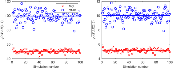
Figure S13: Left plot: Simulation-based estimates of the asymptotic variance of $\hat{\nu}$, i.e. $\sqrt{AVAR_{x}(1,1)}$ for $x=MCL,GMM$, where $AVAR_{x}$ is the asymptotic covariance matrix of $\hat{\theta}$, see Equation (S12.1). Right plot: Simulation-based estimates of the asymptotic variance of $\hat{\lambda}$, i.e. $\sqrt{AVAR_{x}(2,2)}$ for $x=MCL,GMM$. Horizontal lines denote the average over the $100$ simulations.

Appendix S13 Software (MATLAB)

The following functions are available in the MATLAB software language. We give a very brief description of the functions here but refer to the extensive documentation in the code for further details. The code can be freely downloaded from

https://github.com/mbennedsen/Likelihood-based-IVT.

• simulateIVT:

  • Simulates equidistant observations of a parametric IVT process, specified by a Lévy basis and a trawl function. The Lévy basis and trawl function can be specified independently of each other using the framework described in this Supplementary Material.

• estimateIVT:

  • Takes as input a vector of equidistantly spaced observations and a parametric specification (Lévy basis and trawl function) and outputs estimates of the corresponding parameters using the maximum composite likelihood approach developed in the main paper.

• modelselectIVT:

  • This function estimates six parametric IVT models (Poisson-Exponential, Poisson-IG, Poisson-Gamma, NB-Exponential, NB-IG, NB-Gamma) and calculates the composite likelihood function when evaluated in the optimized parameters, as well as the CLAIC and CLBIC criteria given in the main paper. These three criteria can be used for model selection, with larger values indicating a better fit.

• forecastIVT:

  • Takes as input a parametric IVT model (Lévy basis and trawl function), a forecast horizon (which can be a vector of several forecast horizons), as well as historical observations; the output is the predictive probability distribution for the given forecast horizons. The parameters underlying the predictive distribution are estimated using the maximum composite likelihood approach presented in the main paper.

• analyze_stock_A and analyze_simulated_data:

  • These files illustrate the use of the functions simulateIVT, estimateIVT, modelselectIVT, and forecastIVT. The file analyze_stock_A reproduces the output of the main paper, while analyze_simulated_data simulates a user-specified IVT process and then conducts analyses similar to those considered in the main paper on these simulated data.

References

- (1)
- Abramowitz & Stegun (1972) Abramowitz, M. & Stegun, I. A. (1972), Handbook of mathematical functions with formulas, graphs, and mathematical tables, Vol. 55, 10th edn, United States Department of Commerce.
- Al-Osh & Alzaid (1987) Al-Osh, M. A. & Alzaid, A. A. (1987), ‘First-order integer-valued autoregressive (INAR(1)) process’, Journal of Time Series Analysis 8(3), 261–275.
- Andrieu et al. (2010) Andrieu, C., Doucet, A. & Holenstein, R. (2010), ‘Particle Markov chain Monte Carlo methods’, Journal of the Royal Statistical Society: Series B 72, 269–342.
- Barndorff-Nielsen (2011) Barndorff-Nielsen, O. E. (2011), ‘Stationary infinitely divisible processes’, Brazilian Journal of Probability and Statistics 25(3), 294 – 322.

References

- Abramowitz and Stegun (1972) Abramowitz, M. and I. A. Stegun (1972). Handbook of mathematical functions with formulas, graphs, and mathematical tables (10th ed.), Volume 55. United States Department of Commerce.