On Submodular Prophet Inequalities and Correlation Gap

Abstract

Prophet inequalities and secretary problems have been extensively studied in recent years due to their elegance, connections to online algorithms, stochastic optimization, and mechanism design problems in game theoretic settings. Rubinstein and Singla [37] developed a notion of combinatorial prophet inequalities in order to generalize the standard prophet inequality setting to combinatorial valuation functions such as submodular and subadditive functions. For non-negative submodular functions they demonstrated a constant factor prophet inequality for matroid constraints. Along the way they showed a variant of the correlation gap for non-negative submodular functions.

In this paper we revisit their notion of correlation gap as well as the standard notion of correlation gap and prove much tighter and cleaner bounds. Via these bounds and other insights we obtain substantially improved constant factor combinatorial prophet inequalities for both monotone and non-monotone submodular functions over any constraint that admits an Online Contention Resolution Scheme. In addition to improved bounds we describe efficient polynomial-time algorithms that achieve these bounds.

Keywords: prophet inequalities, contention resolution schemes, online algorithms, matroids

1 Introduction

Prophet inequalities arose from stochastic optimization and stopping theory in the ’70s. In the basic setting there are $n$ independent real-valued random variables $X_{1},X_{2},\ldots,X_{n}$ with prescribed distributions $\mathcal{D}_{1},\ldots,\mathcal{D}_{n}$; they correspond to values of some items. An online algorithm (or agent) knows the distributions of the random variables a priori but sees their realizations in an adversarial order, and has to choose exactly one of them. The algorithm has to make an irrevocable decision on whether to accept an item or not when it arrives. In the single item setting the first accepted item stops the process. The algorithm’s performance is measured with respect to the value of a prophet who gets to see all the realizations and then picks the variable with the largest value. The expected value of the prophet is $V^{*}=\mathop{\mathbb{E}}[\max_{i}X_{i}]$. An online algorithm $\alpha$-competitive if its expected value is at least $\alpha V^{*}$. Krengel and Sucheston [34] showed that $1/2$ is the optimal competitive ratio for the single item setting. Secretary problems are closely related to prophet inequalities. In the classical version an online algorithm sees $n$ adversarially chosen values in a random order and has to pick one item irrevocably and compete with the maximum value. A classical result of Dynkin [18] shows an optimal competitive ratio of $1/e$.

There has been substantial recent interest in prophet inequalities and secretary problems in theoretical computer science. Initial interest arose from strong connections to online mechanism design and posted price mechanisms for revenue maximization [29, 12] (see [30, 13] for surveys on Bayesian mechanism design). Subsequent work explored several different variants including prophet inequality and secretary problems in more general settings. Of particular interest to us is the setting where multiple variables/items from $X_{1},X_{2},\ldots,X_{n}$ can be chosen such that the chosen items are feasible in some combinatorial constraint family. Two important examples are choosing $k$ items for some integer $k\geq 1$ [4] and a further generalization where the items chosen are independent in a matroid [33]. These generalizations had several motivations including algorithmic game theory, combinatorial optimization, stochastic optimization, and online algorithms. A rich body of work has emerged with several elegant and useful results. We refer the reader to surveys on prophet inequalities by Lucier [35] and Correa et al. [15], a survey by Dinitz on the secretary problem [16] and by Gupta and Singla generally on random-order models [28], for several pointers to the extensive literature on these problems and related topics.

Combinatorial Prophet Inequalities: Prophet inequalities and secretary problems were mostly studied with modular/additive objective functions, by which we mean that the total value of a subset $S$ of variables is simply the sum of their values. However, more general combinatorial objective functions have many useful applications. By a combinatorial objective we mean that the value of a subset of items from $[n]$ is specified by a set function $f:2^{[n]}\rightarrow\mathbb{R}$. Prominent examples are submodular and subadditive set functions, and their special cases. The secretary problem was studied with submodular objectives and it was shown that it can be reduced to the modular case with a constant factor loss [24]. This motivated Rubinstein and Singla to define a model of combinatorial prophet inequalities which is the main object of study in this paper. We restrict our attention to submodular objectives which form a rich class and, following [37], we refer to this as the Submodular Prophet Inequality (SPI) problem.

The model defined by Rubinstein and Singla is the following elegant generalization of the standard prophet inequality problem. The input consists of $n$ independent random variables $X_{1},X_{2},\ldots,X_{n}$. Unlike the standard prophet inequality where $X_{i}$ is a real-valued random variable, in the combinatorial setting, each $X_{i}$ is a discrete-valued random variable over a finite set $\mathcal{U}_{i}$. Thus $\mathcal{D}_{i}$ is a discrete probability distribution over $\mathcal{U}_{i}$. For technical reasons one assumes that $\mathcal{U}_{1},\mathcal{U}_{2},\ldots,\mathcal{U}_{n}$ are mutually disjoint. Let $\mathcal{U}=\bigcup_{i}\mathcal{U}_{i}$. There is a non-negative submodular function $f:2^{\mathcal{U}}\rightarrow\mathbb{R}_{+}$ defined over the ground set $\mathcal{U}$. As in the standard prophet inequality setting, the variables arrive in an adversarial order. The online algorithm has to make irrevocable decisions about accepting the outcome of a variable after seeing its realization when it arrives, and its goal is to maximize the value $f(S)$ of the selected set $S\subseteq\mathcal{U}$. What about the constraints? Recall that in the standard prophet inequality, the goal is to select a subset of variables from a feasible collection of sets. Similarly, we assume that there is a downward-closed family of sets $\mathcal{I}\subseteq 2^{[n]}$, and it is required that the chosen variables belong to $\mathcal{I}$. We emphasize that $\mathcal{I}$ is defined over $[n]$ and not $\mathcal{U}$. The prophet, which gets to see all the realizations, can optimize offline, and one can see that its expected profit is $\mathop{\mathbb{E}}[\max_{S\in\mathcal{I}}f(\bigcup_{i\in S}\{X_{i}\})]$.

We briefly motivate a scenario for the setup above. First, we observe that the standard prophet inequality with additive functions and arbitrary downward-closed constraints can be modeled by the combinatorial setting. We simply need to approximate a real-valued random variable $X_{i}$, sufficiently closely, by a discrete distribution over point values. This is relatively easy to do for most distributions of interest. Now consider the modeling power of the combinatorial setting. Suppose we have an online advertising situation where one sees on each day (or time slot) a customer of some type drawn from a known distribution. It is natural to assume that customer types are discrete (or can be approximated fairly well by a discrete distribution with a sufficiently large domain). The agency has to irrevocably decide whether to show an ad to the customer when they arrive. The agency has various constraints on the ads that it can show. For instance, there could be a budget constraint which dictates that at most $k$ ads can be shown overall which corresponds to picking $k$ days/variables from the set of $n$ arrivals. What is the value of serving the ads? That depends on the application at hand. Rich objective functions allow substantial flexibility in the ability to model the profit. For instance it is easy to imagine a decreasing marginal utility for showing ads to the same type of customers and this can be easily captured by submodular functions. The model proposed by [37] allows arbitrary submodular functions over the entire universe $\mathcal{U}$, which is fairly powerful. The goal of our description is to point out the generality of the model as it relates to the traditional prophet inequality setting which has already seen many applications.

Rubinstein and Singla showed that one can obtain an $O(1)$-competitive algorithm for SPI when the constraint on selecting the days is a matroid constraint. However, they did not explicitly consider the case of monotone submodular functions and they focused only on a single matroid constraint. Moreover, the constant they obtained is very large (in the thousands, although they did not try to optimize it) and they did not consider or emphasize the computational aspects of the online algorithm. We note that prophet inequalities in the standard setting of modular/additive objectives are fairly small. For instance, the well-known result of Kleinberg and Weinberg [33] showed a bound of $1/2$ even for arbitrary matroid constraints, and it is also known that the bound for a cardinality constraint with $k$ items is $(1-O(1/\sqrt{k}))$ (hence it tends to $1$ as $k\rightarrow\infty$) [4].

Motivation and technical challenges: Our main motivation is to obtain improved bounds for SPI via a clean framework that applies to a wide variety of constraints. This question was explicitly raised by Lucier in his survey on prophet inequalities [35]. Another motivation for this paper, related to the goal of obtaining improved bounds, comes from a technical tool that Rubinstein and Singla relied upon, namely the notion of the correlation gap. One reason for the large constant in their prophet inequality comes from the correlation gap they prove for non-negative submodular functions. In addition to the correlation gap bound, a second technical challenge comes from the model. On each day $i$ a single element from $\mathcal{U}_{i}$ is realized. Thus the overall distribution over $\mathcal{U}$ is correlated. Known rounding schemes for submodular functions such as (Online) Contention Resolution Schemes [14, 23, 2] rely on independence and one needs to suitably adapt them when handling general classes of constraints beyond a single matroid, considered in [37]. We describe the important notion of the correlation gap that is of independent interest beyond the prophet inequality setting.

Correlation gap of non-negative submodular functions: The term correlation gap of a set function was introduced in the work of Agrawal et al. [3] and has since found several applications. For any non-negative real-valued set function $f:2^{\mathcal{N}}\rightarrow\mathbb{R}_{+}$ the correlation gap of $f$ is the worst-case ratio of two continuous extension of $f$, namely the multilinear extension $F$ and the concave closure $f^{+}$ . In probabilistic terms, consider a distribution $\mathcal{D}$ over $\mathcal{N}=[n]$ with marginals given by $\bm{x}\in[0,1]^{n}$. The multilinear extension $F(\bm{x})$ measures the expected value of $f$ under the product distribution with marginals $\bm{x}$. The concave closure $f^{+}(\bm{x})$ gives the maximum expected value of $f$ over all distributions with marginals $\bm{x}$. The ratio $\inf_{\bm{x}\in[0,1]^{n}}\frac{F(\bm{x})}{f^{+}(\bm{x})}$ is the correlation gap. If $f$ is a modular/additive function, it is easy to see that the correlation gap is $1$. An important result in submodular optimization is that the correlation gap is at most $(1-1/e)$ for any monotone submodular function [3, 11, 39]. However, it is known that the correlation gap for general non-negative submodular functions (which can be non-monotone) can be arbitrarily small. Rubinstein and Singla [37] instead use the correlation gap of a related function, namely, $f_{\max}$ defined as follows: $f_{\max}(S)=\max_{T\subseteq S}f(T)$. The function $f_{\max}$ is monotone, but is in general not submodular, even when $f$ is. It is shown in [37] that for any non-negative submodular function $f$, $\inf_{\bm{x}\in[0,1]^{n}}\frac{F_{\max}(\bm{x})}{f^{+}(\bm{x})}\geq 1/200$, where $F_{\max}$ is the multilinear extension of $f_{\max}$. The main technical claim they prove is that $F\left(\frac{1}{2}\bm{x}\right)\geq\frac{1}{200}f^{+}(\bm{x})$ for any $\bm{x}\in[0,1]^{n}$. The proof in [37] relies on existing tools but is involved and goes via another continuous extension. In this paper, we seek to improve the bound but also to give a refined analysis of the correlation gap for non-negative functions via a parameter $p=\max_{i\in\mathcal{N}}x_{i}$.

1.1 Our contributions

In this paper we make two high-level contributions. First, we consider the correlation gap for non-negative submodular functions both in the original definition and in the modified sense of [37] described above. In both cases, we obtain substantially improved bounds. Second, we revisit the SPI problem and address three issues: (i) significantly improved constants for the prophet inequalities for monotone and non-monotone functions, (ii) a clean black-box reduction to greedy Online Contention Resolution Schemes that allows one to obtain prophet inequalities for various other constraints beyond a single matroid constraint and (iii) computational aspects of the prophet inequality that were not explicitly addressed in [37]. In essence, we answer the open question in [35] in the affirmative.

Correlation gap:

For a non-negative submodular function, for any given $p\in[0,1]$, there is a simple instance even when $n=2$ such that $F(\bm{x})\leq(1-p)f^{+}(\bm{x})$ and this implies that, as $p$ tends to $1$, the correlation gap tends to $0$. In particular, it turns out that $p=\max_{i}x_{i}=|\bm{x}|_{\infty}$. This phenomenon manifests itself in non-monotone submodular function maximization in various ways and the typical way to overcome this is to restrict attention to settings where $p$ is away from $1$. Nevertheless, there has been little work on precisely quantifying the correlation gap as a function of this parameter. Our first theorem addresses this.

Theorem 1.1.

Let $f:2^{\mathcal{N}}\rightarrow\mathbb{R}_{\geq 0}$ be a non-negative submodular function and let $\bm{x}\in[0,1]^{n}$, where $n=|\mathcal{N}|$. Let $p=\max_{i}x_{i}$. Then $F(\bm{x})\geq(1-p)(1-1/e)f^{+}(\bm{x})$. Given any $p\in[0,1]$ there are instances such that $F(\bm{x})\leq(1-e^{-(1-p)})f^{+}(\bm{x})$.

The upper bound of $(1-p)(1-1/e)$ is optimal when $p$ is close to $0$ or when $p$ is close to $1$. The lower bound on the gap that we show, $1-e^{-(1-p)}$, agrees nicely with the extremes, but we do not know whether it is the right bound for all ranges of $p$ and leave it as an interesting open problem.

We then consider the correlation gap considered by [37] with respect to the function $f_{\max}$. We observe that known results on the Measured Continuous Greedy (MCG) algorithm [22, 2] show that $F_{\max}(\bm{x})\geq\frac{1}{e}f^{+}(\bm{x})$.

We strengthen this observation by considering the parameter $p$.

Theorem 1.2.

Let $f:2^{\mathcal{N}}\rightarrow\mathbb{R}_{\geq 0}$ be a non-negative submodular function and let $\bm{x}\in[0,1]^{n}$, where $n=|\mathcal{N}|$. Let $p=\max_{i}x_{i}$. There exists a point $\bm{y}\in[0,1]^{n}$, where $\bm{y}\leq\bm{x}$ (coordinate wise), such that $F(\bm{y})\geq\max\{\frac{1}{e},(1-p-\frac{1}{e}(1+\ln(1-p)))\}f^{+}(\bm{x})$.

We obtain the preceding theorem as a corollary of the following more technical theorem.

Theorem 1.3.

Let $p\in[0,1)$, $f$ be a non-negative submodular function with multilinear extension $F$ and $\mathcal{P}$ be a downward-closed solvable polytope on $\mathcal{N}$, such that $\mathcal{P}\subseteq p\cdot[0,1]^{\mathcal{N}}$ (that is, if $\bm{z}\in\mathcal{P}$ then $z_{i}\leq p$ for all $i\in\mathcal{N}$). Then, the output of the Measured Continuous Greedy (MCG) algorithm on $F$ and $\mathcal{P}$ at time $b\in[0,1]$ is a vector $\bm{x}(b)\in b\cdot\mathcal{P}$ such that

$$F(\bm{x}(b))\geq\begin{cases}b\cdot e^{-b}\cdot\max_{\bm{z}\in\mathcal{P}}{f^{+}(\bm{z})},&\text{for }0\leq b\leq\ln{\left(\frac{1}{1-p}\right)}\\ \left(1-p-e^{-b}\left(1+\ln{(1-p)}\right)\right)\cdot\max_{\bm{z}\in\mathcal{P}}{f^{+}(\bm{z})},&\text{for }\ln{\left(\frac{1}{1-p}\right)}\leq b\leq 1.\end{cases}$$

Theorems 1.1 and 1.3 are useful when one has a situation where $p$ is already small and we will see later that this can indeed be achieved in some cases, such as in the SPI problem, via a reduction.

Submodular Prophet Inequality:

For SPI we follow the high level framework of [37] via the correlation gap and greedy Online Contention Resolution Schemes (OCRSs) [23] (see Appendix A.2 for some background and formal definitions). Our main contributions are several technical improvements and refinements that lead to significantly improved constants and, we believe, clarity on the parameters that affect the constants. The competitive ratio that we achieve for a particular constraint family is dictated by the OCRS available for that family. Roughly speaking, an OCRS for a constraint family is an online rounding scheme for a given polyhedral relaxation of the constraints. The approximation quality of the OCRS is governed by two parameters $b,c\in[0,1]$ via the notion of $(b,c)$-selectability. For matroids there is $(b,1-b)$-selectable OCRS for any $b\in[0,1]$, while there is a $(b,e^{-2b})$-OCRS for matching constraints and a $\left(1-\frac{t}{\sqrt{k}},1-\exp(\frac{-t^{2}}{4})\right)$-OCRS for the special case of a uniform matroid of rank $k$ (picking at most $k$ elements); see [23].

Theorem 1.4 (Informal).

For the SPI problem with a monotone function $f$ over a constraint family with a $(b,c)$-selectable OCRS, there is a $c\cdot(e^{-b}-\varepsilon)(1-e^{-b})$-competitive algorithm for any fixed $\varepsilon>0$. For non-negative submodular functions there is a $\frac{c}{4}\cdot(e^{-b}-\varepsilon)(1-e^{-b})$-competitive algorithm for any fixed $\varepsilon>0$. These competitive ratios can be achieved by an efficient randomized polynomial time algorithm, assuming value oracle access to $f$ and efficiency of the corresponding OCRS.

So far we have avoided mentioning the power of the adversary in choosing the order of the variables. Our results hold in the setting of an almighty adversary who can adaptively decide the ordering of the variables based on the full realization of all the variables and the choices of the algorithm at each step. We note that the competitive ratios we obtain are explicit and relatively small. We summarize our concrete competitive ratios for several constraints of interest below. OCRSs for constraints can be composed nicely (similar to CRSs) and our black box reduction is hence very useful.

Feasibility constraint	Competitive Ratio
	Monotone Submodular	General Submodular
Uniform matroid of rank $k\rightarrow\infty$	$1/4.3$	$1/17.2$
Matroid	$1/7.4$	$1/30$
Matching	$1/9.5$	$1/38$
Knapsack	$1/17.5$	$1/70$
Intersection of $k$ matroids	$\Omega(1/k)$	$\Omega(1/k)$

Table 1: A summary of our results for several feasibility constraints.

1.2 Brief overview of technical ideas

Correlation gap: The correlation gap for monotone functions [10, 39] used a continuous time argument by relating $F(\bm{x})$ and $f^{+}(\bm{x})$ via another continuous extension $f^{*}$ and this was the same approach followed in [37]. We take a different approach. For the exact correlation gap in Theorem 1.1 we build on a proof for the monotone case from [14] which is less well-known; we adapt their proof for the non-negative case via the parameter $p$. As we remarked, another approach to bound the correlation gap is via properties of the MCG algorithm. The original papers on the MCG algorithm [11, 22] related the quality of the output to that of the multilinear relaxation. It was only observed later, motivated by stochastic optimization, that the guarantees of these algorithms are stronger and can be shown with respect to the optimum concave closure (see [1, 2]). We build on these to derive Theorem 1.2.

SPI: We follow the high-level approach of [37] but make several technical improvements that we briefly describe. The approach in [37] is to obtain a fractional solution offline and then round it online via a greedy OCRS. There are three technical ingredients. First is the correlation gap; we already discussed our improvements on this issue. Second is the fact that the distribution over $\mathcal{U}_{i}$ on each day is a correlated distribution. Rubinstein and Singla essentially show that the limited correlation in the distribution on each day can be approximately simulated by a product distribution over $\mathcal{U}_{i}$. In this process one loses large constant factors. We show a simple reduction that reduces the original SPI instance to another one in which the probability of any item in $\mathcal{U}_{i}$ being realized can be made arbitrarily small. This allows us to substantially improve the constants in several interrelated ways. Third, [37] rely on the greedy OCRS schemes from [23] in order to round the fractional solution. As we remarked, the constraints are on the days/variables while the objective is defined over $\mathcal{U}$. In [37] the authors implicitly use the fact that the derived constraint on $\mathcal{U}$ is still a matroid constraint, if the original constraint on $\mathcal{N}$ is a matroid. However, this does not generalize to other constraints. One way to handle this is to obtain a new OCRS for the derived constraint over $\mathcal{U}$ from that on $\mathcal{N}$. This would lead to technical difficulties and also lose further constants. In this paper we overcome this difficulty by using the greedy OCRS for $(\mathcal{N},\mathcal{I})$ in a black box fashion. We obtain a clean algorithm that works for any constraint on $\mathcal{N}$ that admits a greedy OCRS. Our analysis relies on opening up the internal properties of a greedy OCRS from [23].

1.3 Other related work

We already referred to recent surveys on prophet inequalities and secretary problems and related models [35, 15, 28, 16]. An older survey on prophet inequalities from a stopping theory point of view is due to Hill and Kertz [31]. The work here is connected to submodular optimization, stochastic optimization, online algorithms, and mechanism design which have extensive literature. It is infeasible to describe all the related work; Singla’s thesis [38] touches upon several of these themes and has several pointers. Contention Resolution Schemes (CRSs) have found many applications since their introduction [14]; in fact Bayesian mechanism design and posted price mechanisms [12] and subesequent work by Yan [40], connecting mechanism design with the correlation gap, played an important role in [14]. Online CRSs were developed [23] with applications to Bayesian mechanism design as one of the main motivations and they yield prophet inequalities in the modular case. Random order CRSs were introduced in [2] and yield improved bounds when the arrival order is random. We discuss a variant of the SPI problem for this setting in more detail in Appendix D. Random Order CRSs found several applications including to (submodular) stochastic probing which has been extensively studied in the past several years [1, 25, 27, 26, 7, 5]. There are some high-level connections between submodular stochastic probing and the SPI model, and it is not too surprising that continuous extensions and CRSs play a role in prior work and ours. However the probing model requires items to be chosen if examined, and thus differs from the prophet inequality model, in which items are allowed to be examined before making the decision. As we remarked already, the SPI model introduces a particular nuance due to correlations which is absent in prior models.

Submodular functions and constraints that we consider such as cardinality, matroids, and others provide generality and computational tractability. It is possible to go beyond and consider more general objective functions such as subadditive and monotone XOS functions, as well as more complex and general independence constraints. In such settings one can ignore computational considerations and focus on the online competitive ratio or assume access to a demand oracle (even though a demand oracle may be NP-Hard in general). We refer to [36, 37] for some recent work and pointers. Such functions have also been considered under the related model of “combinatorial auctions” [19, 17, 6], in which a seller wants to sell distinct items to buyers that have combinatorial valuation functions for the items. The seller wishes to maximize either the social welfare or the revenue. In this model, Dutting, Feldman, Kesselheim and Lucier [19] obtained a $2$ prophet inequality for submodular functions, while Dutting, Kesselheim and Lucier [17] obtained a $O(\log\log m)$ prophet inequality for subadditive functions. For the latter, the authors also show that achieving a constant factor prophet inequality for subadditive valuation functions is impossible via their techniques and requires a different approach.

Organization:

Section 2 sets up technical preliminaries on submodular functions and introduces our notation. Section 3 describes the relaxation of the prophet’s objective. Section 4 describes the algorithm and analysis for SPI. We describe some open questions in Section 5.

For several lemmas on submodular functions and sampling used throughout the paper, see Appendix A.1. For background information on contention resolution schemes, see Appendix A.2. The proofs of Theorems 1.1 and 1.3 have been moved to Appendix B due to space constraints. The reduction to small probabilities can be found in Appendix C. Appendix D contains a discussion on a variant of the SPI problem, the SPS problem, in which the random variables arrive uniformly at random instead of in adversarial order.

2 Preliminaries

Let $\mathcal{N}$ be a finite ground set. A real-valued set function $f:\{0,1\}^{\mathcal{N}}\to\mathbb{R}_{\geq 0}$ is called submodular if, for all $A,B\subseteq\mathcal{N}$, it satisfies $f(A)+f(B)\geq f(A\cup B)+f(A\cap B)$. $f$ is monotone if $f(A)\leq f(B)$ for all $A\subseteq B$. In the rest of this paper we work with non-negative normalized functions that satisfy $f(\emptyset)=0$ and $f(A)\geq 0$ for all $A\subseteq\mathcal{N}$. We often equate $\mathcal{N}$ with $[n]=\{1,2,\ldots,n\}$. We use the terminology $S+i$ and $S-i$ as shorthands for $S\cup\{i\}$ and $S\setminus\{i\}$ respectively. The following continuous extensions of submodular functions to $[0,1]^{\mathcal{N}}$ play an important role in our discussion.

Definition 2.1 (Multilinear Extension).

Let $f:{\{0,1\}}^{\mathcal{N}}\to\mathbb{R}_{\geq 0}$. For any $\bm{x}\in{[0,1]}^{n}$, let $S\sim\bm{x}$ denote a random set $S$ that contains each element $i\in\mathcal{N}$ independently w.p. $x_{i}$. The multilinear extension of $f$ is defined as

$$F(\bm{x})\coloneqq\mathop{\mathbb{E}}_{S\sim\bm{x}}[f(S)]=\sum_{S\subseteq N}{f(S)\prod_{i\in S}{x_{i}}\prod_{i\notin S}{(1-x_{i})}}.$$

Definition 2.2 (Concave Closure).

Let $f:{\{0,1\}}^{\mathcal{N}}\to\mathbb{R}_{\geq 0}$. Moreover, let $\mathbbm{1}_{S}$ denote the characteristic vector of length $n=|\mathcal{N}|$. For any $\bm{x}\in{[0,1]}^{n}$, the concave closure of $f$ is defined as

$$f^{+}(\bm{x})\coloneqq\max_{\bm{a}\in[0,1]^{2^{\mathcal{N}}}}\left\{\sum_{S\subseteq\mathcal{N}}{a_{S}f(S)}\>\middle|\>\sum_{S\subseteq\mathcal{N}}{a_{S}}=1,\sum_{S\subseteq\mathcal{N}}{a_{S}\mathbbm{1}_{S}}=\bm{x}\right\}.$$

Recall that $f^{+}(\bm{x})$ can be interpreted as the maximum expected value of $f(R)$ where $R$ is generated by a distribution whose marginal values are given by $\bm{x}$. Since $F(\bm{x})$ corresponds to the product distribution defined by $\bm{x}$, which is a specific distribution, it follows that $F(\bm{x})\leq f^{+}(\bm{x})$ for all $\bm{x}$.

We also need the following notation, which will be useful in our analysis when dealing with the input constraints.

Definition 2.3 (Blowup of a Ground Set).

Let $\mathcal{N}$ denote a finite set. Suppose for each $e\in\mathcal{N}$ there is an associated finite non-empty set $A_{e}$ such that the sets $A_{e},e\in\mathcal{N}$ are mutually disjoint. Let $\mathcal{A}=\{A_{e}\mid e\in N\}$. We call $\mathcal{N}^{\prime}=\bigcup_{e\in N}A_{e}$ the blowup of $\mathcal{N}$ by $\mathcal{A}$.

Recall that each day only one item from $\mathcal{U}_{i}$ is realized and this motivates the following definition of a constraint family.

Definition 2.4 (Partition Extension of a Constraint).

Let $\mathcal{C}=(\mathcal{N},\mathcal{I})$ be a downward-closed constraint family over $\mathcal{N}$. Consider a blowup $\mathcal{N}^{\prime}$ of $\mathcal{N}$ induced by sets $A_{e},e\in\mathcal{N}$. Consider the function $g:\mathcal{N}^{\prime}\rightarrow\mathcal{N}$ where $g(e^{\prime})=e$ if and only if $e^{\prime}\in A_{e}$. The partition extension of $\mathcal{C}$, denoted by $\mathcal{C}^{\prime}$, is a constraint family $(\mathcal{N}^{\prime},\mathcal{I}^{\prime})$ where

$$\mathcal{I}^{\prime}_{A}=\left\{S\subseteq\mathcal{N}^{\prime}\>\middle|\>g(S)\in\mathcal{I}\text{ and }\forall e\in\mathcal{N},\>|A_{e}\cap S|\leq 1\right\}.$$

3 Submodular Prophet Inequality Problem

In the Submodular Prophet Inequality (SPI) problem, we are given $n$ random variables $X_{1},\dots,X_{n}$ following (known) distributions $D_{1},\dots,D_{n}$, along with a constraint $\mathcal{C}$ on $\mathcal{N}=\{1,2,\dots,n\}$. The random variables are arranged in adversarial (worst-case) order. Let $\mathcal{U}_{i}$ denote the image (range) of $X_{i}$, and $\mathcal{I}$ denote the independent sets of $\mathcal{C}$.

The online algorithm starts with a set $S=\emptyset$ of selected elements and a set $Z=\emptyset$ of selected days. At the $i$-th time step, it is presented with the realization $e\in\mathcal{U}_{i}$ of $X_{i}$. At that moment, it has to decide irrevocably whether to include $e$ in $S$ (and hence $i$ in $Z$) or not, subject to $Z$ remaining independent in $\mathcal{C}$. The algorithm is also given a non-negative submodular function $f:\mathcal{U}\to\mathbb{R}_{\geq 0}$, where $\mathcal{U}\triangleq\bigcup_{i=1}^{n}{\mathcal{U}_{i}}$. The algorithm’s objective is to maximize $f(S)$, subject to $Z$ being independent in $\mathcal{C}$.

In this model, we are comparing against the almighty adversary who already knows all realizations and can adaptively change the order in which to reveal the random variables based on the algorithm’s actions so far and also the random coins it uses (if the algorithm is randomized). The prophet/adversary will select the best possible set $S^{*}$ according to the constraints with knowledge of the realizations. Thus, we compare the expected value of the online algorithm against the expected value of the prophet, which is

$${\rm OPT}=\mathop{\mathbb{E}}_{\bm{X}}\left[\max_{T\in\mathcal{I}}f\left(\left\{X_{i}\>\middle|\>i\in T\right\}\right)\right].$$

Later, we will use an OCRS to round the fractional solution we obtain in this section. Since $f$ is defined over $\mathcal{U}$ but the constraint given is over $\mathcal{N}$, the days, we cannot immediately apply an OCRS for rounding. To overcome this issue, we view $\mathcal{U}$ as the blowup of $\mathcal{N}$ with respect to $\left\{\mathcal{U}_{i}\right\}_{i=1}^{n}$. On each day $i$, only one element arrives. Therefore, our input constraint $\mathcal{C}$ is equivalent to a new constraint $\mathcal{C}^{\prime}$ on $\mathcal{U}$, where we are allowed to pick only one element from each day. Notice that this is exactly the partition extension $\mathcal{C}^{\prime}=(\mathcal{U},\mathcal{I}^{\prime})$ of $\mathcal{C}$.

We also denote $\bm{X}=\left\{X_{1},X_{2},\dots,X_{n}\right\}$ and $\bm{D}=\left\{D_{1},D_{2},\dots,D_{n}\right\}$. For an element $e\in\mathcal{U}_{i}$ we let $D_{i}(e)$ denote the probability of $e$ being realized; we also use the notation $\mathcal{D}(e)$ to denote the probability of $e\in\mathcal{U}$ when we do not need to specify the part it belongs to. Note that the elements within $\mathcal{U}_{i}$ are correlated and hence we do not have a product distribution on $\mathcal{U}$.

Algorithmic approach:

Following the description in Section 1, we design an online algorithm following the general approach of [37] but with technical differences. First, we obtain a relaxation of the prophet’s objective. Afterwards, to design an online algorithm, we obtain an offline fractional point $\bm{z}$ based on the input, and round it online using a greedy OCRS and other tools. In this section, we describe the relaxation of the prophet’s objective and how to obtain an offline fractional point $\bm{z}$. The process of rounding $\bm{z}$ online using a greedy OCRS is presented in Section 4.

Before we proceed, we describe a simple but technically important reduction that allows us to obtain improved bounds.

Observation 3.1 (Reduction to small probabilities).

Let $I=(\mathcal{N},\mathcal{U},\bm{D},\bm{X},f,\mathcal{C})$ be an instance of the Submodular Prophet Inequality problem. For every fixed $\varepsilon>0$, there is a reduction of $I$ to another instance $I^{\prime}=(\mathcal{N},\mathcal{U}^{\prime},\bm{D^{\prime}},\bm{Y},g,\mathcal{C})$ of the SPI problem such that that (i) for all $e\in\mathcal{U}^{\prime}$, $\bm{D^{\prime}}(e)\leq\varepsilon$ and (ii) there exists an $\alpha$-competitive algorithm for $I$ if and only if there exists an $\alpha$-competitive algorithm for $I^{\prime}$.

Remark 3.2.

The reduction’s simplicity may make the reader wonder why it is useful in achieving improved bounds. The reason is a combination of the model and the power of submodularity. The fact that we can only pick a single random variable from each day allows us to make copies of the elements, and we can use a derived submodular function to treat the copies as a single element.

We describe the reduction in Appendix C, but only sketch its correctness since it is rather simple and easy to see, though tedious to formally prove. The reduction to small probabilities allows us to use improved correlation gaps, as well as obtain better bounds in the rounding algorithm.

3.1 An upper bound on the prophet’s value:

Let $\mathcal{P}$ denote a solvable polyhedral relaxation of $\mathcal{C}$ . Then one can easily develop a solvable polyhedral relaxation of $\mathcal{C}^{\prime}$ as follows:

$$\mathcal{P}^{\prime}=\left\{\bm{y}\in[0,1]^{|\mathcal{U}|}\>\middle|\>\sum_{e\in\mathcal{U}_{i}}y_{e}=x_{i},\,\,\,i\in[n],\bm{x}\in\mathcal{P}\right\}.$$

Consider any algorithm, including an offline algorithm, that computes a feasible output given the realizations of the random variables. For any fixed algorithm $\mathcal{A}$ (deterministic or randomized) we have a probability $p_{\mathcal{A}}(e)$ for each $e\in\mathcal{U}$ appearing in the output of $\mathcal{A}$. Since an element $e\in\mathcal{U}$ is realized with probability $\mathcal{D}(e)$, $e$ cannot appear in the output of $\mathcal{A}$ with probability more than $\mathcal{D}(e)$. Moreover, for a given realization, each output of the algorithm is feasible. Putting these facts together we obtain the following observation.

Observation 3.3.

Let $\mathcal{A}$ be any online or offline algorithm for a given instance of the problem. Let $p_{\mathcal{A}}(e)$ denote the probability that $e$ is in the output of $\mathcal{A}$. Then the vector $\bm{p}$ is in the polytope

$$\mathcal{P}^{\prime\prime}=\left\{\bm{z}\in[0,1]^{|\mathcal{U}|}\>\middle|\>\bm{z}\in\mathcal{P}^{\prime},z_{e}\leq\mathcal{D}(e)\,\,e\in\mathcal{U}\right\}.$$

We are now ready to proceed with the relaxation of the prophet’s objective.

Claim 3.4.

Consider an instance of the Submodular Prophet Inequality problem. Then

$$\max_{\bm{z}\in\mathcal{P}^{\prime\prime}}{f^{+}(\bm{z})}\geq{\rm OPT}.$$

Proof.

Fix an optimal strategy for the prophet and let $\bm{y^{*}}\in[0,1]^{|\mathcal{U}|}$ denote the vector of probabilities of the elements appearing in the output of the prophet’s strategy. We have $\bm{y^{*}}\in\mathcal{P}^{\prime\prime}$. By the definition of the concave closure of $f$, $f^{+}(\bm{y^{*}})$ maximizes the value of $f$ among all distributions with the marginals $\bm{y^{*}}$ (note that the distribution that achieves this may not be a feasible strategy for any algorithm). Therefore, $f^{+}(\bm{y^{*}})\geq{\rm OPT}$, which also implies that $\max_{\bm{z}\in\mathcal{P}^{\prime\prime}}{f^{+}(\bm{z})}\geq{\rm OPT}$. ∎

3.2 Fractional Solution and Correlation Gap

From Claim 3.4, $\max_{\bm{z}\in\mathcal{P}^{\prime\prime}}{f^{+}(\bm{z})}\geq{\rm OPT}$. Since OCRSs are designed to relate the quality of their output to that of the multilinear relaxation, we need to relate $F(\bm{z})$ to $f^{+}(\bm{z})$ and hence to ${\rm OPT}$. We present two different ways to do this — via a direct correlation gap and via the Measured Continuous Greedy (MCG) algorithm — with the second yielding strictly better results than the first.

The direct correlation gap approach

The first approach is not computationally efficient and relies on optimally solving the optimization problem $\max_{\bm{z}\in\mathcal{P}^{\prime\prime}}{f^{+}(\bm{z})}$. Let $\bm{z^{*}}$ be the optimum solution. We can then use the correlation gap to relate $F(\bm{z^{*}})$ to ${\rm OPT}$. For monotone functions we have $F(\bm{z^{*}})\geq(1-1/e)f^{+}(\bm{z^{*}})\geq(1-1/e){\rm OPT}$. For non-negative functions we can use Theorem 1.1, the proof of which, along with all results on the direct correlation gap approach, can be found in Appendix B. Following the reduction that we described earlier, we can assume that $z_{e}^{*}\leq\max_{e}\bm{D}(e)\leq\varepsilon$ for all $e$ and this implies, via Theorem 1.1 that $F(\bm{z^{*}})\geq(1-\varepsilon)(1-1/e)f^{+}(\bm{z^{*}})\geq(1-\varepsilon)(1-1/e){\rm OPT}$. In rounding it is useful to have a solution $\bm{z}\in b\cdot\mathcal{P}^{\prime\prime}$ for some parameter $b\in(0,1)$. One can of course use $\bm{z}=b\bm{z^{*}}$ and in this case, we can use the concavity of $f^{+}$ to see that $f^{+}(b\bm{z^{*}})\geq bf^{+}(\bm{z^{*}})$, and then apply the correlation gap to $b\bm{z^{*}}$ to conclude that, in the monotone case, $F(b\bm{z^{*}})\geq b(1-1/e)f^{+}(\bm{z^{*}})\geq b(1-1/e){\rm OPT}$ and, in the non-monotone case, $F(b\bm{z^{*}})\geq b(1-\varepsilon)(1-1/e)f^{+}(\bm{z^{*}})\geq b(1-\varepsilon)(1-1/e){\rm OPT}$.

The measured continuous greedy approach

The second approach is algorithmic and relies on the Measured Continuous Greedy (MCG) algorithm and its properties. We state two relevant known results about the algorithm. For these results as well as Theorem 1.3, we assume the submodular function $f$ is given via a value oracle, and that the algorithms are randomized and run in polynomial time and are correct with high probability.

Lemma 3.5 (Lemma 4 of [1]).

Let $f$ be a monotone submodular function with multilinear extension $F$, and let $\mathcal{P}$ be a solvable downward-closed polytope. Let $\bm{x}(b)$ be solution produced by the Continuous Greedy algorithm on $F$ and $\mathcal{P}$ until time $b\in(0,1]$. Then (i) $\bm{x}(b)\in b\cdot\mathcal{P}$ and (ii) $F(\bm{x}(b))\geq\left(1-e^{-b}-o(1)\right)\cdot\max_{\bm{y}\in\mathcal{P}}{f^{+}(\bm{y})}$.

For a general non-negative submodular function, the MCG algorithm achieves the following bound.

Lemma 3.6 (Lemma 8.3 of [2]).

Let $b\in[0,1]$, $f$ be a non-negative submodular function with multilinear extension $F$, and let $\mathcal{P}$ be a solvable downward-closed polytope. Then, the solution $\bm{x}(b)\in{[0,1]}^{n}$ produced by the MCG algorithm satisfies (i) $\bm{x}(b)\in b\cdot\mathcal{P}$ and (ii) $F(\bm{x}(b))\geq\left(b\cdot e^{-b}-\varepsilon\right)\cdot\max_{\bm{y}\in\mathcal{P}}{f^{+}(\bm{y})}$, for any fixed $\varepsilon>0$.

The two preceding lemmas are algorithmic. If $\mathcal{P}$ is solvable then the underlying algorithms can be implemented efficiently. Based on our reduction to small probabilities it is useful to consider whether the preceding lemmas can take advantage of this. No advantage is possible in the monotone setting, however, we show below that one can indeed take advantage of the reduction when $f$ is non-monotone. We provide a refined analysis of the standard bound of the MCG algorithm, which depends on a parameter $p$ that quantifies the maximum value of any coordinate that is feasible in the polytope. For small enough $p$, Theorem 1.3 constitutes an improvement over Lemma 3.6, which comprises the main result of this section. We restate the theorem here, while its proof can be found in Appendix B. Notice that Theorem 1.2 follows from Theorem 1.3 by setting $b=1$.

See 1.3

Remark 3.7.

Notice that, for the SPI problem, due to our reduction, we can assume that all vectors $\bm{z}\in\mathcal{P}^{\prime\prime}$ have $z_{i}\leq\varepsilon^{\prime}$ for all $i\in\mathcal{N}$, for any fixed constant $\varepsilon^{\prime}>0$. Therefore, for any fixed constant $\varepsilon>0$, there exists an $\varepsilon^{\prime}$ such that

$$F(\bm{x}(b))\geq\left(1-e^{-b}-\varepsilon\right)\cdot\max_{\bm{z}\in\mathcal{P}}{f^{+}(\bm{z})},$$

where $\bm{x}(b)\in b\cdot\mathcal{P}^{\prime\prime}$ is the output of the MCG algorithm at time $b$.

We summarize the results via both methods below. We observe that for both monotone and non-monotone functions the bounds are best when $p\rightarrow 0$, which we can ensure via the reduction. Once we make this assumption, the bounds provided by the correlation gap approach are essentially $(1-1/e)$ when $b=1$ which is optimal. However, these bounds are matched by the Continuous Greedy approach. When $b<1$, which will be the case when applying the rounding schemes, the bound in Lemma 3.5 and our new refined bound in Theorem 1.3 are superior and have the further advantage of being computable in polynomial time.

4 Rounding the fractional solution

In the preceding section we described ways to obtain a vector $\bm{z}\in b\cdot\mathcal{P}^{\prime\prime}$ for some $b\in[0,1]$ such that $F(\bm{z})\geq\alpha\cdot OPT$ for various constants $\alpha$ depending on the approach. In this section we show how to round $\bm{z}$ in an online fashion. We follow the high-level approach of [37] but refine it in several ways. We will use a greedy OCRS for $\mathcal{C}$ via the relaxation $\mathcal{P}$ as a black box. Recall that our rounding needs to produce a feasible set in $\mathcal{C}^{\prime}$ with ground set $\mathcal{U}$, while the OCRS is for the constraint on days/variables $\mathcal{N}$. Moreover the distribution $\bm{D}$ is not a product distribution on $\mathcal{U}$. These are the technical challenges that need to be overcome in the algorithm and analysis. The quality of the output will depend on the properties of the OCRS for $\mathcal{P}$. We assume that the greedy OCRS for $\mathcal{P}$ is $(b,c)$-selectable, where $c$ is some function of $b$. This depends on the specific constraint family $\mathcal{C}$ and the polyhedral relaxation $\mathcal{P}$. At the end of the section, we use known results to derive concrete competitive ratios for several constraint families of interest. We note that $\bm{z}\in\mathcal{P}^{\prime\prime}$, which also implies that $\bm{z}\in\mathcal{P}^{\prime}$. For rounding purposes we only work with $\mathcal{P}^{\prime}$ and $\mathcal{P}$; $\mathcal{P}^{\prime\prime}$ is only necessary to obtain an upper bound on ${\rm OPT}$.

We rely on the certain parts of the analysis of OCRS for submodular function maximization from [23]. In the following, we will use $\pi$ to denote the mapping function for the OCRS over the ground set $\mathcal{N}$ and the polytope $\mathcal{P}$. Technically the mapping $\pi$ is a function of $\bm{x}\in\mathcal{P}$ and should be written as $\pi_{\bm{x}}$ but we omit $\bm{x}$ for notational simplicity. We also note that $\pi$ can be randomized. An important definition from [23] in the analysis of OCRSs is the characteristic CRS of a greedy OCRS.

Definition 4.1 (Characteristic CRS of an OCRS).

The characteristic CRS $\bar{\pi}$ of a greedy OCRS $\pi$ for a polytope $\mathcal{P}$ is a CRS for the same polytope $\mathcal{P}$. It is defined for an input $x\in\mathcal{P}$ and a set $A\subseteq\mathcal{N}$ by $\bar{\pi}(A)=\left\{e\in A\>\middle|\>I\cup\{e\}\in\mathcal{F}_{\pi,\bm{x}},\>\>\forall I\subseteq A,\>I\in\mathcal{F}_{\pi,\bm{x}}\right\}$. Notice that, if $\pi$ is randomized, then $\bar{\pi}$ is randomized as well.

We will also need the following known results from [23].

Observation 4.2 (Observation 3.3 of [23]).

For every set $A\subseteq\mathcal{N}$ and a characteristic CRS $\bar{\pi}$ of a greedy OCRS $\pi$, the set $\bar{\pi}(A)$ is always a subset of the elements selected by $\pi$ when the active elements are the elements of $A$.

Lemma 4.3 (Lemma 3.4 of [23]).

The characteristic CRS $\bar{\pi}$ of a $(b,c)$-selectable greedy OCRS $\pi$ is $(b,c)$-balanced and monotone.

For any $S\subseteq\mathcal{U}$, we define $S_{\downarrow}\subseteq\mathcal{N}$ to be the projection of $S$ onto $\mathcal{N}$, i.e.

$$S_{\downarrow}\coloneqq\left\{i\in\mathcal{N}\>\middle|\>S\cap\mathcal{U}_{i}\neq\emptyset\right\}.$$

Also, for a greedy OCRS $\pi$, we denote the characteristic CRS of $\pi$ by $\bar{\pi}$. We now define a CRS $\pi^{\prime}$ for $\mathcal{P}^{\prime}$ that we will need for our analysis later on. We define $\pi^{\prime}$ using the characteristic CRS $\bar{\pi}$ of $\pi$ as follows. For any set $S\subseteq\mathcal{U}$,

$$\pi^{\prime}(S)\coloneqq\bigcup_{{\begin{subarray}{c}i\in\bar{\pi}(S_{\downarrow})\\ |S\cap\mathcal{U}_{i}|=1\end{subarray}}}{(S\cap\mathcal{U}_{i})}.$$

Lemma 4.4.

For any $(b,c)$-selectable greedy OCRS $\pi$ for $\mathcal{P}$ and $\bm{z}\in\mathcal{P}^{\prime}$, the mapping $\pi^{\prime}$ is is a $(b,c\cdot\gamma)$-balanced monotone CRS $\pi^{\prime}$ for $\mathcal{P}^{\prime}$, where $\gamma=\min_{i\in\mathcal{N}}{\prod_{e\in\mathcal{U}_{i}}{(1-z_{e})}}$.

Proof.

First, notice that $\pi^{\prime}$ is a CRS, since $\pi^{\prime}(S)\subseteq S$ for all $S\subseteq\mathcal{U}$. This follows immediately from the definition of $\pi^{\prime}$ as $S\cap\mathcal{U}_{i}\subseteq S$ for all $i\in\mathcal{N},S\subseteq\mathcal{U}$.

Next, we show that $\pi^{\prime}$ is monotone. Fix an element $e\in S_{1}\subseteq S_{2}\subseteq\mathcal{U}$, and an instantiation of $\mathcal{F}_{\pi,\bm{x}}$ (this is relevant if the OCRS is randomized). Let $e\in\mathcal{U}_{i}$ for some $i\in\mathcal{N}$. Suppose $e\in\pi^{\prime}(S_{2})$. This implies that $|S_{2}\cap\mathcal{U}_{i}|=1$ and since $S_{1}\subseteq S_{2}$ and $e\in S_{1}$, we have $|S_{1}\cap\mathcal{U}_{i}|=1$. Furthermore, we know that $i\in\bar{\pi}({S_{2}}_{\downarrow})$. Since $S_{1}\subseteq S_{2}$, it follows that ${S_{1}}_{\downarrow}\subseteq{S_{2}}_{\downarrow}$. By Lemma 4.3, we know that $\bar{\pi}$ is monotone, and thus, since $i\in\bar{\pi}({S_{2}}_{\downarrow})$, it follows that $i\in\bar{\pi}({S_{1}}_{\downarrow})$. Therefore, we know that $e\in\pi^{\prime}(S_{1})$. Since $e\in\pi^{\prime}(S_{2})$ implies that $e\in\pi^{\prime}(S_{1})$, unconditioning over the instantiation of $\mathcal{F}_{\pi,\bm{x}}$ yields

$$\Pr\left[e\in\pi^{\prime}(S_{1})\right]\geq\Pr\left[e\in\pi^{\prime}(S_{2})\right].$$

We now show that $\pi^{\prime}$ is $(b,c\cdot\gamma)$-balanced, for $\gamma=\min_{i\in\mathcal{N}}{\prod_{e\in\mathcal{U}_{i}}{(1-z_{e})}}$. It suffices to show that, for any $e\in\mathcal{U}$

$$\Pr_{S\sim R(\bm{z})}\left[e\in\pi^{\prime}(S)\>\middle|\>e\in S\right]\geq c\cdot\gamma.$$

Notice that, for any realization $S$ of $R(\bm{z})$, $e\in\pi^{\prime}(S)$ if and only if $S\cap\mathcal{U}_{i}=\{e\}$ and $i\in\bar{\pi}(S_{\downarrow})$. Thus,

$$\Pr_{S\sim R(\bm{z})}\left[e\in\pi^{\prime}(S)\>\middle|\>e\in S\right] =\Pr_{S\sim R(\bm{z})}\left[S\cap\mathcal{U}_{i}=\{e\}\wedge i\in\bar{\pi}(S_{\downarrow})\>\middle|\>e\in S\right]$$

$$=\Pr_{S\sim R(\bm{z})}\left[S\cap\mathcal{U}_{i}=\{e\}\>\middle|\>e\in S\right]$$

$$\qquad\cdot\Pr_{S\sim R(\bm{z})}\left[i\in\bar{\pi}(S_{\downarrow})\>\middle|\>S\cap\mathcal{U}_{i}=\{e\},e\in S\right]$$

$$=\Pr_{S\sim R(\bm{z})}\left[S\cap\mathcal{U}_{i}=\{e\}\>\middle|\>e\in S\right]$$

$$\qquad\cdot\Pr_{S\sim R(\bm{z})}\left[i\in\bar{\pi}(S_{\downarrow})\>\middle|\>S\cap\mathcal{U}_{i}=\{e\}\right],$$ (1)

where the last equality follows from the fact that, if $S\cap\mathcal{U}_{i}=\{e\}$, then $e\in S$. We lower bound each probability in (1) separately, starting from

$$\Pr_{S\sim R(\bm{z})}\left[S\cap\mathcal{U}_{i}=\{e\}\>\middle|\>e\in S\right]=\prod_{e^{\prime}\neq e,e^{\prime}\in\mathcal{U}_{i}}{(1-z_{e^{\prime}})}\geq\prod_{e^{\prime}\in\mathcal{U}_{i}}{(1-z_{e^{\prime}})}\geq\gamma.$$ (2)

Also, notice that $\bar{\pi}$ is a CRS over $\mathcal{N}$ and does not depend on which $S\cap\mathcal{U}_{i}$ led to $i\in S_{\downarrow}$. Therefore,

$$\Pr\left[i\in\bar{\pi}(S_{\downarrow})\>\middle|\>i\in S_{\downarrow}\right]=\Pr\left[i\in\bar{\pi}\>\middle|\>S\cap\mathcal{U}_{i}=T\right]$$

for all $T\subseteq\mathcal{U}_{i}$ such that $T\neq\emptyset$. Specifically, for $T=\{e\}$,

$$\Pr\left[i\in\bar{\pi}\>\middle|\>S\cap\mathcal{U}_{i}=\{e\}\right]=\Pr\left[i\in\bar{\pi}(S_{\downarrow})\>\middle|\>i\in S_{\downarrow}\right]\geq c,$$ (3)

where the last inequality follows from the fact that fact that $\bar{\pi}$ is $(b,c)$-balanced, by Lemma 4.3.

Combining (1), (2) and (3), we obtain

$$\Pr_{S\sim R(\bm{z})}\left[e\in\pi^{\prime}(S)\>\middle|\>e\in S\right]\geq c\cdot\gamma.$$

∎

Remark 4.5.

Notice that via Observation 3.1, we can assume without loss of generality that, for any fixed $\varepsilon^{\prime}>0$, $z_{e}\leq\varepsilon^{\prime}$ for all $e\in\mathcal{U}$. By choosing $\varepsilon^{\prime}$ sufficiently small, for any fixed $\varepsilon>0$ we have

$$\gamma=\min_{i\in\mathcal{N}}{\prod_{e\in\mathcal{U}_{i}}{(1-z_{e})}}\geq\min_{i\in\mathcal{N}}{\left(\prod_{e\in\mathcal{U}_{i}}{e^{-z_{e}}}\right)}-\varepsilon=\min_{i\in\mathcal{N}}{\left(e^{-\sum_{e\in\mathcal{U}_{i}}{z_{e}}}\right)}-\varepsilon\geq e^{-b}-\varepsilon,$$

where the last inequality follows from the fact that $\bm{z}\in b\cdot\mathcal{P}^{\prime}$. Thus, $c\cdot\gamma\geq c\cdot(e^{-b}-\varepsilon)$, and we obtain the following as corollary: For any $(b,c)$-selectable greedy OCRS $\pi$ for $\mathcal{P}$ and fixed $\varepsilon>0$, $\pi^{\prime}$ defined earlier is a $\left(b,c\left(e^{-b}-\varepsilon\right)\right)$-balanced monotone CRS for $\mathcal{P}^{\prime}$.

Now we are ready to describe our online algorithm. We describe and analyze the algorithms for monotone and non-monotone cases separately, since there are technical differences. The algorithms are similar to the one in [37], however, the main technical difference is that we use the OCRS for $\mathcal{N}$ as a black box; in [37] the authors use an OCRS over $\mathcal{U}$ since they work in the special case of matroids.

4.1 Monotone Non-Negative Submodular Functions

We assume we have already computed a vector $\bm{z}\in b\cdot\mathcal{P}^{\prime\prime}$ for some $b\in[0,1]$ such that $F(\bm{z})\geq\alpha\cdot{\rm OPT}$ for some $\alpha$. Note that the adversary is almighty and can alter the order in which it feeds the variables to the algorithm based on knowledge of the full realizations of the variables and the actions of the algorithm so far.

Let $\bm{z_{i}}$ denote the product distribution on $\mathcal{U}_{i}$ defined by marginals $z_{i}(e),e\in\mathcal{U}_{i}$. We write $R\sim\bm{z_{i}}$ to denote a random set $R\subseteq\mathcal{U}_{i}$ realized according to this product distribution, and we denote $z_{i}(e)$ by $z_{e}$ when $i$ is clear from context or irrelevant. Furthermore, let $\bm{x}\in[0,1]^{n}$ be the vector where $x_{i}=\Pr_{R\sim\bm{z_{i}}}\left[R\neq\emptyset\right]=1-\prod_{e\in\mathcal{U}_{i}}{(1-z_{e})}$, for all $i\in\mathcal{N}$. We assume that $\bm{x}$ is the input vector to our OCRS $\pi_{x}$ for $\mathcal{P}$ and its characteristic CRS $\bar{\pi}_{\bm{x}}$. To simplify our notation, we denote $\pi_{\bm{x}}$ and $\bar{\pi}_{\bm{x}}$ by $\pi$ and $\bar{\pi}$, respectively.

Monotone Rounding$\left(\mathcal{U},f,\bm{D},\mathcal{C},\pi,\bm{z}\right)$

$T_{\text{ALG}}=\emptyset$

for $h\leftarrow 1$ to $n$ do

       Let $X_{i}$ be variable that arrives on day $h$

       Let $e\in\mathcal{U}_{i}$ be the realization of $X_{i}$

       With probability $\frac{\Pr_{R\sim\bm{z_{i}}}\left[R=\{e\}\right]}{\mathcal{D}_{i}(e)}$, set $T_{i}\leftarrow\{e\}$

       Otherwise, set $T_{i}$ to be a random subset $R$ of $\mathcal{U}_{i}$, drawn according to $\bm{z}_{i}$, conditioned on $|R|\neq 1$

       if $T_{i}\neq\emptyset$ then

             Feed $i$ to OCRS $\pi$ for $\mathcal{P}$

             if $\pi$ accepts $i$ and $T_{i}=\{e\}$ then

                   $T_{\text{ALG}}\leftarrow T_{\text{ALG}}\cup\{e\}$

             end if

            

       end if

      

end for

Return $T_{\text{ALG}}$

ALGORITHM 1 Algorithm for Monotone Non-Negative Submodular Functions

The online algorithm on the $h$-th day receives a random variable $X_{i}$ decided by the almighty adversary, and once $X_{i}$ is received the algorithm also sees the realization $e\in\mathcal{U}_{i}$ of $X_{i}$ according to the distribution $\mathcal{D}_{i}$. The online algorithm generates a random set $T_{i}\subseteq\mathcal{U}_{i}$ after seeing the realization $e$. The idea is that if one does not see the realization $e$ of $X_{i}$, the distribution of $T_{i}$ appears identical to the product distribution generated by $\bm{z_{i}}$. Note that, for $S\subseteq\mathcal{U}_{i}$, $\Pr_{R\sim\bm{z_{i}}}[R=S]=\prod_{e\in S}z_{e}\prod_{e\in\mathcal{U}\setminus S}\left(1-z_{e}\right)$.

Lemma 4.6.

For any $i\in\mathcal{N}$ and $S\subseteq\mathcal{U}_{i}$,

$$\Pr[T_{i}=S]=\Pr_{R\sim\bm{z_{i}}}[R=S].$$

Proof.

Let $\mathcal{E}_{e}$ be the event that $e\in\mathcal{U}_{i}$ is the realization of $X_{i}$. Note that $\Pr[\mathcal{E}_{e}]=\mathcal{D}_{i}(e)$. Consider $S\subseteq\mathcal{U}_{i}$ such that $|S|\neq 1$. We see from the algorithm’s description that

$$\Pr[T_{i}=S\mid\mathcal{E}_{e}]=\left(1-\frac{\Pr_{R}\left[R\left(\bm{z}_{i}\right)=\{e\}\right]}{D_{i}(e)}\right)\cdot\frac{\Pr_{R}\left[R\left(\bm{z}_{i}\right)=S\right]}{1-\Pr_{R}\left[|R\left(\bm{z}_{i}\right)|=1\right]}.$$

Summing up over all realizations of $X_{i}$, we have that, for any $S$ such that $|S|\neq 1$,

$$\Pr\left[T_{i}=S\right] =\sum_{e\in\mathcal{U}_{i}}{D_{i}(e)\Pr\left[T_{i}=S\>\middle|\>\mathcal{E}_{e}\right]}$$

$$=\sum_{e\in\mathcal{U}_{i}}{D_{i}(e)\left(1-\frac{\Pr_{R}\left[R\left(\bm{z}_{i}\right)=\{e\}\right]}{D_{i}(e)}\right)\cdot\frac{\Pr_{R}\left[R\left(\bm{z}_{i}\right)=S\right]}{1-\Pr_{R}\left[|R\left(\bm{z}_{i}\right)|=1\right]}}$$

$$=\frac{\Pr_{R}\left[R\left(\bm{z}_{i}\right)=S\right]}{1-\Pr_{R}\left[|R\left(\bm{z}_{i}\right)|=1\right]}\cdot\sum_{e\in\mathcal{U}_{i}}{D_{i}(e)\left(1-\frac{\Pr_{R}\left[R\left(\bm{z}_{i}\right)=\{e\}\right]}{D_{i}(e)}\right)}$$

$$=\frac{\Pr_{R}\left[R\left(\bm{z}_{i}\right)=S\right]}{1-\Pr_{R}\left[|R\left(\bm{z}_{i}\right)|=1\right]}\cdot\left(\sum_{e\in\mathcal{U}_{i}}{D_{i}(e)}-\sum_{e\in U_{i}}{\Pr_{R}\left[R\left(\bm{z}_{i}\right)=\{e\}\right]}\right)$$

$$=\frac{\Pr_{R}\left[R\left(\bm{z}_{i}\right)=S\right]}{1-\Pr_{R}\left[|R\left(\bm{z}_{i}\right)|=1\right]}\cdot\left(1-\sum_{e\in\mathcal{U}_{i}}{\Pr_{R}\left[R\left(\bm{z}_{i}\right)=\{e\}\right]}\right)$$

$$=\frac{\Pr_{R}\left[R\left(\bm{z}_{i}\right)=S\right]}{1-\Pr_{R}\left[|R\left(\bm{z}_{i}\right)|=1\right]}\cdot\left(1-\Pr_{R}\left[|R\left(\bm{z}_{i}\right)|=1\right]\right)$$

$$=\Pr_{R}\left[R\left(\bm{z}_{i}\right)=S\right].$$

Next, consider any set $S$ with $|S|=1$ and, without loss of generality, assume $S=\{e\}$ for some $e\in\mathcal{U}_{i}$. It can be seen from the algorithm description that $T_{i}=\{e\}$ if and only if $e$ is the realization of $X_{i}$ and the algorithm succeeds in Line 5 in setting $T_{i}=\{e\}$ which happens with probability $\frac{\Pr_{R\sim\bm{z_{i}}}\left[R=\{e\}\right]}{\mathcal{D}_{i}(e)}$. Hence

$$\Pr[T_{i}=\{e\}]=\mathcal{D}_{i}(e)\cdot\frac{\Pr_{R\sim\bm{z_{i}}}\left[R=\{e\}\right]}{\mathcal{D}_{i}(e)}=\Pr_{R\sim\bm{z_{i}}}\left[R=\{e\}\right],$$

as desired. ∎

We now analyze the expected value of $f(T_{\text{ALG}})$ relying on the CRS $\pi^{\prime}$ that we set up (this is inspired by the use of characteristic CRS in [23]).

Lemma 4.7.

Given a $(b,c)$-selectable greedy OCRS $\pi$ for $\mathcal{P}$, for any $\bm{z}\in b\cdot\mathcal{P}^{\prime\prime}$ and fixed $\varepsilon>0$, Algorithm 1 returns a set $T_{\text{ALG}}\subseteq\mathcal{U}$ such that

$$\mathop{\mathbb{E}}\left[f(T_{\text{ALG}})\right]\geq c\left(e^{-b}-\varepsilon\right)\cdot F(\bm{z}).$$

Proof.

It is easy to see from the algorithm’s description that, for any $X_{i}$, only the actual realization of $X_{i}$ can be potentially chosen to be added to $T_{\text{ALG}}$. Furthermore, the variables chosen by the algorithm are feasible in $\mathcal{C}$, since this is ensured by the OCRS.

Let $T_{i}$ be the random set generated by the online algorithm for variable $X_{i}$. We see that $T_{i}$ is independent of $T_{i^{\prime}}$ for $i\neq i^{\prime}$, due to independence of the realization of the random variables $X_{1},\ldots,X_{n}$ and the independence of the coins used in the algorithm across days. From Lemma 4.6, the distribution of $T_{i}$ is according to the product distribution $R\sim\bm{z_{i}}$ over $\mathcal{U}_{i}$. Let $Q=\bigcup_{i=1}^{n}T_{i}$. It follows that $Q$ is a random set drawn from the product distribution induced by $\bm{z}$ over $\mathcal{U}$. Consider the distribution of the set $Q_{\downarrow}\in\mathcal{N}$. Because of the product distribution of $Q$ it can be see that the distribution of $Q_{\downarrow}$ is a product distribution on $\mathcal{N}$ where $i\in\mathcal{N}$ appears in $Q_{\downarrow}$ with probability $x_{i}=1-\prod_{e\in\mathcal{U}_{i}}(1-z_{e})\leq b$ since $z\in b\cdot\mathcal{P}^{\prime\prime}$. Note that the algorithm feeds $Q_{\downarrow}$ to the OCRS $\pi$ which is $(b,c)$-selectable. Let $\bar{\pi}$ be the characteristic CRS of $\pi$.

Fix a realization $S$ of $Q$, along with an instantiation of $\mathcal{F}_{\pi,\bm{x}}$. Notice $e\in T_{\text{ALG}}\cap\mathcal{U}_{i}$ if and only if $|S\cap\mathcal{U}_{i}|=\{e\}$ and $i\in\pi(S_{\downarrow})$. In fact,

$$T_{\text{ALG}}=\bigcup_{{\begin{subarray}{c}i\in\pi(S_{\downarrow})\\ |S\cap\mathcal{U}_{i}|=1\end{subarray}}}{(S\cap\mathcal{U}_{i})},$$

by the description of Algorithm 1. By Observation 4.2, we have $\bar{\pi}(A)\subseteq\pi(A)$ for any $A\subseteq\mathcal{N}$, and thus $\pi^{\prime}(S)\subseteq T_{\text{ALG}}$. Therefore, by the monotonicity of $f$, we have $f\left(T_{\text{ALG}}\right)\geq f\left(\pi^{\prime}(S)\right)$, and by unconditioning

$$\mathop{\mathbb{E}}\left[f\left(T_{\text{ALG}}\right)\right]\geq\mathop{\mathbb{E}}\left[f\left(\pi^{\prime}(Q)\right)\right].$$

Finally, by Lemma 4.4 and Remark 4.5, we have that for any $\bm{z}\in b\cdot\mathcal{P}^{\prime\prime}$ and any fixed $\varepsilon>0$,

$$\mathop{\mathbb{E}}\left[f\left(\pi^{\prime}(Q)\right)\right]\geq c\left(e^{-b}-\varepsilon\right)\cdot F(\bm{z}),$$

which yields

$$\mathop{\mathbb{E}}\left[f\left(T_{\text{ALG}}\right)\right]\geq c\left(e^{-b}-\varepsilon\right)\cdot F(\bm{z}).$$

∎

We are now ready for the main theorem of this section, which follows from Lemmas 4.7 and 3.5, and Claim 3.4.

Theorem 4.8.

Let $(\mathcal{N},\bm{D},\mathcal{C},f)$ be an instance of the Submodular Prophet Inequality model and let $OPT$ denote the prophet’s value. Given a $(b,c)$-selectable greedy OCRS $\pi$ for $\mathcal{P}$, for a non-negative monotone submodular function $f$, $\bm{z}\in b\cdot\mathcal{P}^{\prime\prime}$ and fixed $\varepsilon>0$, Algorithm 1 returns a set $T_{\text{ALG}}$ such that

$$\mathop{\mathbb{E}}\left[f(T_{\text{ALG}})\right]\geq c\left(e^{-b}-\varepsilon\right)\left(1-e^{-b}\right)\cdot{\rm OPT}.$$

Next, we provide concrete results for several constraints, given an OCRS for these constraints. First, we summarize known greedy OCRSs for various constraints of interest below.

Lemma 4.9 (Theorem 1.1 from [23]).

There exist:

• For every $b\in[0,1]$, a $(b,1-b)$-selectable deterministic greedy OCRS for matroid polytopes.

• For every $b\in[0,1]$, a $(b,e^{-2b})$-selectable randomized greedy OCRS for matching polytopes.

• For every $b\in[0,\frac{1}{2}]$, a $(b,\frac{1-2b}{2-2b})$-selectable randomized greedy OCRS for the natural relaxation of a knapsack constraint.

By combining Lemma 4.9 with Theorem 4.8, we obtain the following corollary.

Corollary 4.10.

Let $(\mathcal{N},\bm{D},\mathcal{C},f)$ be an instance of the Submodular Prophet Inequality model and let $OPT$ denote the prophet’s value. For a non-negative monotone submodular function $f$ and any fixed $\varepsilon>0$, Algorithm 1 returns a set $T_{\text{ALG}}$ such that

$$\mathop{\mathbb{E}}_{\bm{X},\mathcal{T}}[f(T_{\text{ALG}})] \geq(1-b)\left(e^{-b}-\varepsilon\right)\left(1-e^{-b}\right)\cdot OPT, \forall b\in[0,1],\text{ if }\mathcal{C}\text{ is a matroid constraint}$$

$$\mathop{\mathbb{E}}_{\bm{X},\mathcal{T}}[f(T_{\text{ALG}})] \geq e^{-2b}\left(e^{-b}-\varepsilon\right)\left(1-e^{-b}\right)\cdot OPT, \forall b\in[0,1],\text{ if }\mathcal{C}\text{ is a matching constraint}$$

$$\mathop{\mathbb{E}}_{\bm{X},\mathcal{T}}[f(T_{\text{ALG}})] \geq\frac{1-2b}{2-2b}\left(e^{-b}-\varepsilon\right)\left(1-e^{-b}\right)\cdot OPT, \forall b\in\left[0,\frac{1}{2}\right],\text{ if }\mathcal{C}\text{ is a knapsack constraint}$$

where $\mathcal{T}=\{T^{1},\dots,T^{n}\}$ denotes the set of random sets Algorithm 1 generates.

4.2 Non-Negative Submodular Functions

Below we describe the algorithm for non-negative functions. It is very similar to the monotone case except for a minor change in accepting an element $e$; in the final step, the algorithm tosses an additional random coin and accepts $e$ with probability $1/2$ (see Line 10 in the algorithm). This is inspired by the similar idea in [23] in handling non-monotone functions.

General Rounding$\left(\mathcal{U},f,\bm{D},\mathcal{C},\pi,\bm{z}\right)$

$T_{\text{ALG}}=\emptyset$

for $h\leftarrow 1$ to $n$ do

       Let $X_{i}$ be variable that arrives on day $h$

       Let $e\in\mathcal{U}_{i}$ be the realization of $X_{i}$

       With probability $\frac{\Pr_{R\sim\bm{z_{i}}}\left[R=\{e\}\right]}{\mathcal{D}_{i}(e)}$, set $T_{i}\leftarrow\{e\}$

       Otherwise, set $T_{i}$ to be a random subset $R$ of $\mathcal{U}_{i}$, drawn according to $\bm{z}_{i}$, conditioned on $|R|\neq 1$

       if $T_{i}\neq\emptyset$ then

             Feed $i$ to OCRS $\pi$ for $\mathcal{P}$

             if $\pi$ accepts $i$ and $T_{i}=\{e\}$ then

                   With probability $\frac{1}{2}$, $T_{\text{ALG}}\leftarrow T_{\text{ALG}}\cup\{e\}$

             end if

            

       end if

      

end for

Return $T_{\text{ALG}}$

ALGORITHM 2 Algorithm for General Non-Negative Submodular Functions

Notice that Lemmas 4.4 and 4.6 still hold, as they do not depend on the monotonicity of $f$. We present the following analogue of Lemma 4.7 for general submodular functions. The proof of the next lemma relies on an argument similar to that in [23].

Lemma 4.11.

Given a $(b,c)$-selectable greedy OCRS $\pi$ for $\mathcal{P}$, for any $\bm{z}\in b\cdot\mathcal{P}^{\prime\prime}$ and fixed $\varepsilon>0$, Algorithm 2 returns a set $T_{\text{ALG}}\subseteq\mathcal{U}$ such that

$$\mathop{\mathbb{E}}\left[f(T_{\text{ALG}})\right]\geq\frac{c\left(e^{-b}-\varepsilon\right)}{4}\cdot F(\bm{z}).$$

Proof.

At every step $i$, Algorithm 2 draws a random set $T_{i}$ according to the product distribution on $\mathcal{U}_{i}$ with probabilities $\bm{z_{i}}$, by Lemma 4.6. Let $Q=\bigcup_{i\in\mathcal{N}}{T_{i}}$. Since the realizations between days are independent, $Q$ is a random set that follows the product distribution on $\mathcal{U}$ with probabilities $\bm{z}$. Fix a realization $S$ of $Q$ and an instantiation of $\mathcal{F}_{\pi,\bm{x}}$. Notice that $e\in T_{\text{ALG}}\cap\mathcal{U}_{i}$ if and only if $|S\cap\mathcal{U}_{i}|=1$, $i\in\pi(S_{\downarrow})$ and the coin toss of Line 10 succeeds. In fact, if we denote

$$W=\bigcup_{{\begin{subarray}{c}i\in\pi(S_{\downarrow})\\ |S\cap\mathcal{U}_{i}|=1\end{subarray}}}{(S\cap\mathcal{U}_{i})},$$

we have that $\mathop{\mathbb{E}}\left[f(T_{\text{ALG}})\right]=\mathop{\mathbb{E}}[f(W(1/2))]$, by the description of Algorithm 2. By Observation 4.2, we have $\bar{\pi}(A)\subseteq\pi(A)$ for any $A\subseteq\mathcal{N}$, and thus $\pi^{\prime}(S)\subseteq W$. For ease of notation, we denote $\pi^{\prime}(S)$ by $L$. For our fixed choice of $S$ and $\mathcal{F}_{\pi,\bm{x}}$, $L$ is deterministic. Therefore, we can think of $W(1/2)$ as obtained by first calculating a set $L(1/2)$ in which every element of $L$ appears with probability $1/2$ independently, and then adding to it a random set $\Delta\subseteq\mathcal{U}\setminus L$. The almighty prophet can control the order in which the elements arrive, and thus can make the distribution of $\Delta$ depend on $L(1/2)$. However, $\Delta$ is guaranteed to contain every element with probability at most $1/2$, for every given realization of $L(1/2)$. Thus,

$$\mathop{\mathbb{E}}\left[f(W(1/2))\>\middle|\>S,\mathcal{F}_{\pi,\bm{x}}\right] =\mathop{\mathbb{E}}\left[f(L(1/2)\cup\Delta)\>\middle|\>S,\mathcal{F}_{\pi,\bm{x}}\right]$$

$$=\sum_{B\subseteq L}{\Pr\left[L(1/2)=B\>\middle|\>S,\mathcal{F}_{\pi,\bm{x}}\right]\cdot\mathop{\mathbb{E}}\left[f(B\cup\Delta)\>\middle|\>S,\mathcal{F}_{\pi,\bm{x}}\right]}$$

$$\geq\sum_{B\subseteq L}{\Pr\left[L(1/2)=B\>\middle|\>S,\mathcal{F}_{\pi,\bm{x}}\right]\cdot\frac{\mathop{\mathbb{E}}\left[f(B)\>\middle|\>S,\mathcal{F}_{\pi,\bm{x}}\right]}{4}}$$

$$=\frac{\mathop{\mathbb{E}}\left[f(L(1/2))\>\middle|\>S,\mathcal{F}_{\pi,\bm{x}}\right]}{2}$$

$$=\frac{\mathop{\mathbb{E}}\left[f(L)\>\middle|\>S,\mathcal{F}_{\pi,\bm{x}}\right]}{4},$$

where the first inequality follows from Lemma A.1 since the function $h_{B}(T)=h(B\cup T)$ is non-negative and submodular for all $B\subseteq\mathcal{U}$, and the second inequality follows from Lemma A.2. Taking an expectation over all possible realizations of $S$ and $\mathcal{F}_{\pi,\bm{x}}$, we obtain

$$\mathop{\mathbb{E}}\left[f(W(1/2))\right]=\mathop{\mathbb{E}}_{S,\mathcal{F}_{\pi,\bm{x}}}\left[\mathop{\mathbb{E}}\left[f(W(1/2))\>\middle|\>S,\mathcal{F}_{\pi,\bm{x}}\right]\right]\geq\mathop{\mathbb{E}}_{S,\mathcal{F}_{\pi,\bm{x}}}\left[\frac{\mathop{\mathbb{E}}\left[f(L)\>\middle|\>S,\mathcal{F}_{\pi,\bm{x}}\right]}{4}\right]=\frac{\mathop{\mathbb{E}}\left[f(L)\right]}{4}.$$

Finally, by Lemma 4.4 and Remark 4.5, we have that for any $\bm{z}\in b\cdot\mathcal{P}^{\prime\prime}$ and any fixed $\varepsilon>0$,

$$\frac{\mathop{\mathbb{E}}\left[f(L)\right]}{4}\geq\frac{c\left(e^{-b}-\varepsilon\right)}{4}\cdot F(\bm{z}),$$

which implies

$$\mathop{\mathbb{E}}\left[f(T_{\text{ALG}})\right]=\mathop{\mathbb{E}}\left[f(W(1/2))\right]\geq\frac{c\left(e^{-b}-\varepsilon\right)}{4}\cdot F(\bm{z}).$$

∎

We are now ready to proceed with the main result for general submodular functions, which follows from Lemma 4.11, Theorem 1.3, and Claim 3.4.

Theorem 4.12.

Let $(\mathcal{N},\bm{D},\mathcal{C},f)$ be an instance of the Submodular Prophet Inequality model and let $OPT$ denote the prophet’s value. Given a $(b,c)$-selectable greedy OCRS $\pi$ for $\mathcal{P}$, for a non-negative submodular function $f$, $\bm{z}\in b\cdot\mathcal{P}^{\prime\prime}$ and fixed $\varepsilon>0$, Algorithm 2 returns a set $T_{\text{ALG}}$ such that

$$\mathop{\mathbb{E}}\left[f(T_{\text{ALG}})\right]\geq\frac{c\left(e^{-b}-\varepsilon\right)}{4}\cdot\left(1-e^{-b}-\varepsilon\right)\cdot OPT.$$

By combining Lemma 4.9 with Theorem 4.12, we obtain the following corollary.

Corollary 4.13.

Let $(\mathcal{N},\bm{D},\mathcal{C},f)$ be an instance of the Submodular Prophet Inequality model and let $OPT$ denote the prophet’s value. For a non-negative submodular function $f$ and any fixed $\varepsilon>0$, Algorithm 2 returns a set $T_{\text{ALG}}$ such that

$$\mathop{\mathbb{E}}[f(T_{\text{ALG}})] \geq\frac{(1-b)\left(e^{-b}-\varepsilon\right)}{4}\cdot\left(1-e^{-b}-\varepsilon\right)\cdot OPT, \forall b\in[0,1],\text{ if }\mathcal{C}\text{ is a matroid constraint}$$

$$\mathop{\mathbb{E}}[f(T_{\text{ALG}})] \geq\frac{e^{-2b}\left(e^{-b}-\varepsilon\right)}{4}\cdot\left(1-e^{-b}-\varepsilon\right)\cdot OPT, \forall b\in[0,1],\text{ if }\mathcal{C}\text{ is a matching constraint}$$

$$\mathop{\mathbb{E}}[f(T_{\text{ALG}})] \geq\frac{(1-2b)\left(e^{-b}-\varepsilon\right)}{8-8b}\cdot\left(1-e^{-b}-\varepsilon\right)\cdot OPT, \forall b\in\left[0,\frac{1}{2}\right],\text{ if }\mathcal{C}\text{ is a knapsack constraint}$$

where $\mathcal{T}=\{T^{1},\dots,T^{n}\}$ denotes the set of random sets Algorithm 1 generates.

5 Conclusion

We presented a general framework for submodular prophet inequalities in the model of [37] via greedy Online Contention Resolution Schemes and correlation gaps. The framework yields substantially improved constant factor competitive ratios for both monotone and general submodular functions, and can be implemented in polynomial time for many classes of interesting constraints. The framework resolves the open question posed in [35] regarding the model of [37].

Along the way, we strengthened the notion of correlation gap for non-negative submodular functions introduced in [37], and provided a fine-grained variant of the standard correlation gap. For both cases, our bounds are cleaner and tighter. Moreover, we presented a refined analysis of the Measured Continuous Greedy algorithm for polytopes with small coordinates and general non-negative submodular functions, showing that, for these cases, it yields a bound that matches the bound of Continuous Greedy for the monotone case.

An interesting open question is whether our fine-grained correlation gap for general non-negative submodular functions can be made tight. It is tempting to conjecture that the lower bound on the gap shown in Theorem B.4 is tight for all values of $p$. We leave this as an interesting open problem to resolve. It is also interesting to obtain further improvements in the bounds we showed for SPI. Of particular interest is the cardinality constraint.

Acknowledgements:

The authors thank Sahil Singla for clarifications on [37]. CC thanks Vondrák and VL thanks Maria Siskaki, Kesav Krishnan and Venkata Sai Bavisetty for helpful discussions.

Appendix A Background on Submodularity and Contention Resolution Schemes

A.1 Useful Lemmas

Below we state several relevant lemmas regarding sampling and submodular functions that we need.

Lemma A.1 (Lemma 2.2 from [9]).

Let $f:2^{\mathcal{N}}\to\mathbb{R}_{\geq 0}$ be submodular. Denote by $A(p)$ a random subset of $A$ where each element appears with probability at most $p$ (not necessarily independently). Then,

$$\mathop{\mathbb{E}}[f(A(p))]\geq(1-p)\cdot f(\emptyset).$$

Lemma A.2 (Lemma 2.2 from [39]).

Let $g:2^{\mathcal{N}}\to\mathbb{R}_{\geq 0}$ be submodular. Denote by $A(p)$ a random subset of $A$ where each element appears with probability exactly $p$ (not necessarily independently). Then

$$\mathop{\mathbb{E}}[g(A(p))]\geq(1-p)\cdot g(\emptyset)+p\cdot g(A).$$

Lemma A.3 (Lemma 2.3 from [39]).

Let $f:2^{\mathcal{N}}\to\mathbb{R}_{\geq 0}$ be submodular, $A,B\subseteq\mathcal{N}$ two (not necessarily disjoint) sets and $A(p),B(q)$ their independently sampled subsets, where each element of $A$ appears in $A(p)$ with probability $p$ and each element of $B$ appears in $B(q)$ with probability $q$. Then

$$\mathop{\mathbb{E}}[f(A(p)\cup B(q))]\geq(1-p)(1-q)\cdot f(\emptyset)+p(1-q)\cdot f(A)+(1-p)q\cdot f(B)+pq\cdot f(A\cup B).$$

Lemma A.4 (Lemma 4.3 from [39]).

Let $f:2^{\mathcal{N}}\to\mathbb{R}_{\geq 0}$ be a submodular function, let $A_{1},A_{2},\dots,A_{k}\subseteq\mathcal{N}$ be $k$ (not necessarily disjoint) sets and let $A_{1}(p_{1}),A_{2}(p_{2}),\dots,A_{k}(p_{k})$ their independently sampled subsets, where each element of $A_{i}$ appears in $A_{i}(p_{i})$ with probability $p_{i}$, for all $1\leq i\leq k$. Then

$$\mathop{\mathbb{E}}\left[f\left(\bigcup_{i=1}^{k}A_{i}(p_{i})\right)\right]\geq\sum_{I\subseteq[k]}{\left(\prod_{j\in I}{p_{j}}\prod_{j\notin I}{(1-p_{j})}f\left(\bigcup_{j\in I}{A_{j}}\right)\right)}.$$

The next Lemma appears in [14], but its proof is slightly obfuscated within Lemma B.2. For clarity, we present it here on its own.

Lemma A.5 ([14]).

Let $a_{1}\geq\dots\geq a_{m}\in\mathbb{R}_{\geq 0}$, and $q_{1},\dots,q_{m}\in[0,1]$ such that $\sum_{k=1}^{m}{q_{k}}=1$. Then

$$\sum_{k=1}^{m}{q_{k}\>a_{k}\prod_{j=1}^{k-1}{(1-q_{j})}}\geq\left(1-\frac{1}{e}\right)\cdot\sum_{j=1}^{m}{q_{j}a_{j}}.$$

Proof.

Since the above inequality is linear in the parameters $a_{i}$, it suffices to prove it for the special case $a_{1}=a_{2}=\dots=a_{r}=1$ and $a_{r+1}=\dots=a_{m}=0$. (A general decreasing sequence of $a_{j}$ can be obtained as a positive linear combination of such special cases). Hence, it remains to prove

$$\sum_{k=1}^{r}{q_{k}\prod_{j=1}^{k-1}{(1-q_{j})}}\geq\left(1-\frac{1}{e}\right)\cdot\sum_{j=1}^{r}{q_{j}}.$$

We start from the left-hand side, which we expand to

$$\sum_{k=1}^{r}{q_{k}\prod_{j=1}^{k-1}{(1-q_{j})}}=1-\prod_{k=1}^{r}{(1-q_{k})}\geq 1-{\left(1-\frac{1}{r}\sum_{k=1}^{r}{q_{k}}\right)}^{r},$$

where the inequality follows from the arithmetic-geometric mean inequality. Finally, we use the concavity of $\phi_{r}(x)\coloneqq 1-{\left(1-\frac{x}{r}\right)}^{r}$, and the fact that $\phi_{r}(0)=0$, to get

$$\phi_{r}(x)\geq\phi_{r}(1)\cdot x=\left(1-{\left(1-\frac{1}{r}\right)}^{r}\right)\cdot x$$

for $x\in[0,1]$. Since $\left(1-{\left(1-\frac{1}{r}\right)}^{r}\right)\geq\left(1-\frac{1}{e}\right)$ for all $r$, we get

$$\phi_{r}(x)\geq\left(1-\frac{1}{e}\right)\cdot x.$$

which implies that

$$\phi_{r}\left(\sum_{k=1}^{r}{q_{k}}\right)=1-{\left(1-\frac{1}{r}\sum_{k=1}^{r}{q_{k}}\right)}^{r}\geq\left(1-\frac{1}{e}\right)\cdot\sum_{k=1}^{r}{q_{k}}.$$

∎

A.2 Constraints and rounding via Contention Resolution Schemes

Let $\mathcal{N}$ be a finite ground set. A constraint family over $\mathcal{N}$ is simply a subset $\mathcal{I}\subseteq 2^{\mathcal{N}}$; a set $S\in\mathcal{I}$ is called feasible, while a set $S\not\in\mathcal{I}$ is called infeasible. We are interested only in downward-closed families of constraints; $\mathcal{I}$ is downward-closed if and only if $A\in\mathcal{I}$ implies that any set $B\subset A$ is also in $\mathcal{I}$. Classical examples of downward-closed families include those induced by a matroid on $\mathcal{N}$ or intersections of several matroids on $\mathcal{N}$, independent sets of graphs, matchings in graphs and hypergraphs, boolean vectors that satisfy packing constraints of the form $A\bm{x}\leq b$ for non-negative $A,b$, among many others. We will use the terminology $(\mathcal{N},\mathcal{I})$ to indicate a constraint family. The maximum weight independent set problem over $(\mathcal{N},\mathcal{I})$ is the following: given $w:\mathcal{N}\rightarrow\mathbb{R}$ solve $\max_{S\in\mathcal{I}}w(S)$ where $w(S)=\sum_{e\in\mathcal{N}}w(e)$. Since many of these problems are NP-Hard, a common technique is to use polyhedral (or more generally convex) relaxations. We say $\mathcal{P}\subseteq[0,1]^{\mathcal{N}}$ is a polyhedral relaxation of $(\mathcal{N},\mathcal{I})$ if $\mathcal{P}$ is a polyhedron and $\mathbbm{1}_{S}\in\mathcal{P}$ for all $S\in\mathcal{I}$ (here $\mathbbm{1}_{S}$ is the characteristic vector of $S$). We say that $\mathcal{P}$ is solvable if one can efficiently do linear optimization over $\mathcal{P}$, that is, given $w:\mathcal{N}\rightarrow\mathbb{R}$, there is a polynomial time algorithm that computes $\max_{\bm{x}\in\mathcal{P}}\sum_{i}w_{i}x_{i}$. Via the multilinear relaxation, the polyhedral approach to approximation has been extended successfully to submodular function maximization [11, 14, 8].

Contention Resolution Schemes:

These are rounding schemes introduced in [14] for submodular function maximization.

Definition A.6 (Contention Resolution Scheme).

Let $b,c\in[0,1]$. A $(b,c)$-balanced Contention Resolution Scheme $\pi$ for $\mathcal{P}_{\mathcal{I}}$ is a procedure that for every $\bm{x}\in b\cdot\mathcal{P}_{\mathcal{I}}$ and $A\subseteq\mathcal{N}$, returns a random set $\pi_{\bm{x}}(A)\subseteq A\cap\text{support}(\bm{x})$ and satisfies the following properties:

1. $\pi_{\bm{x}}(A)\in\mathcal{I}$ with probability $1,\quad\forall A\subseteq\mathcal{N},\bm{x}\in b\cdot\mathcal{P}_{\mathcal{I}}$, and

2. for all $i\in\text{support}(\bm{x})$, $\Pr\left[i\in\pi_{\bm{x}}(R(\bm{x}))\>\middle|\>i\in R(\bm{x})\right]\geq c,\quad\forall\bm{x}\in b\cdot\mathcal{P}_{\mathcal{I}}$.

The scheme is said to be monotone if $\Pr\left[i\in\pi_{\bm{x}}(A_{1})\right]\geq\Pr\left[i\in\pi_{\bm{x}}(A_{2})\right]$ whenever $i\in A_{1}\subseteq A_{2}$.

CRSs are offline rounding schemes. Online Contention Resolution Schemes (OCRS) were introduced by Feldman, Svensson and Zenklusen [23] to handle online settings such as the SPI problem where the arrival order of the elements is adversarial. Random Order Contention Resolution Schemes (ROCRS) were introduced by [2] to handle the cases where the arrival of the elements is a uniformly random permutation.

Definition A.7 (Online Contention Resolution Scheme (OCRS)).

Let us consider the following online selection setting. A point $\bm{x}\in\mathcal{P}$ is given and let $R(\bm{x})$ be a random subset of active elements. The elements $e\in\mathcal{N}$ reveal one by one whether they are active, i.e., $e\in R(\bm{x})$, and the decision whether to select an active element is taken irrevocably before the next element is revealed. An Online Contention Resolution Scheme for $\mathcal{P}$ is an online algorithm that selects a subset $I\subseteq R(\bm{x})$ such that $\mathbbm{1}_{I}\in\mathcal{P}$.

Monotonicity of a CRS is important for rounding the multilinear relaxation of submodular functions [14], although such a condition is not needed for modular functions. In the online setting, [23] defines the notion of a greedy OCRS which is helpful in rounding for submodular functions.

Definition A.8 (Greedy OCRS).

Let $\mathcal{P}\subseteq{[0,1]}^{n}$ be a relaxation for the feasible sets $\mathcal{F}\subseteq 2^{\mathcal{N}}$. A greedy OCRS $\pi$ for $\mathcal{P}$ is an OCRS that for any $\bm{x}\in\mathcal{P}$ defines a down-closed subfamily of feasible sets $\mathcal{F}_{\pi,\bm{x}}\subseteq\mathcal{F}$, and an element $e$ is selected when it arrives if, together with the already selected elements, the obtained set is in $\mathcal{F}_{\pi,\bm{x}}$. If the choice of $\mathcal{F}_{\pi,\bm{x}}$ given $\bm{x}$ is randomized, we talk about a randomized greedy OCRS; otherwise, we talk about a deterministic greedy OCRS.

For a greedy OCRS, the quality of the approximation guaranteed with respect to the multilinear relaxation is governed by the notion of $(b,c)$-selectability [23].

Definition A.9 ($(b,c)$-selectability).

Let $b,c\in[0,1]$. A greedy OCRS for $\mathcal{P}$ is $(b,c)$-selectable if for any $\bm{x}\in b\cdot\mathcal{P}$, we have

$$\Pr\left[I\cup\{e\}\in\mathcal{F}_{\pi,\bm{x}}\quad\forall I\subseteq R(\bm{x}),\>I\in\mathcal{F}_{\pi,\bm{x}}\right]\geq c,\quad\forall e\in\mathcal{N}.$$

Appendix B Correlation Gap for Non-Negative Submodular Functions

In this section we prove Theorems 1.1 and 1.3 on the correlation gap for non-negative submodular functions. Theorem 1.1 is a direct approach to the correlation gap, whereas Theorem 1.3 utilizes the Measured Continuous Greedy algorithm. The proofs of the theorems are qualitatively different and we present them in separate sections.

B.1 Proof of Theorem 1.1

We split the proof into two parts, the upper bound and the lower bound, state them separately and give their proof.

Upper bound:

As we remarked in Section 1, the proof of this upper bound is inspired by the proof in [14] for the monotone case, which is different from the earlier one in [39].

Theorem B.1.

Let $f:2^{\mathcal{N}}\to\mathbb{R}_{\geq 0}$ be a non-negative submodular function, where $n=|\mathcal{N}|$. Let $\bm{x}\in{[0,1]}^{n}$, such that $\bm{x}\leq p\cdot\bm{1}_{\mathcal{N}}$ for some $p\in[0,1]$. Then,

$$F(\bm{x})\geq(1-p)\left(1-\frac{1}{e}\right)f^{+}(\bm{x}).$$

Proof.

Consider a basic feasible solution ${(q_{j},A_{j})}_{j\in[m]}$ to the linear program that defines $f^{+}(\bm{x})$. In other words, $f^{+}(\bm{x})=\sum_{j=1}^{m}{q_{j}f(A_{j})}$, where $\sum_{j=1}^{m}{q_{j}}=1$, $\sum_{j:i\in A_{j}}{q_{j}}=x_{i}$, for all $i$, and $q_{j}\geq 0$ for all $j$. Notice that, since we chose a basic feasible solution and the LP that defines $f^{+}(\bm{x})$ has only $n+1$ constraints, apart from the non-negativity constraints, we have $m\leq n+1$.

Next, consider the following process to generate a subset of elements. For each $j\in[m]$ sample independently each element of $A_{j}$ with probability $q_{j}$. An element $i\in\mathcal{N}$ is not selected with probability equal to $\prod_{j:i\in A_{j}}{(1-q_{j})}$, thus, $i$ is selected with probability equal to $1-\prod_{j:i\in A_{j}}{(1-q_{j})}$. Notice that we can assume without loss of generality that $q_{j}\neq 1$ for all $j$; if $q_{j}=1$ for some $j$ then that implies that $x_{i}=1$ for every element $i\in A_{j}$, and $q_{j^{\prime}}=0$ for all $j^{\prime}\neq j$, which then leads us to $F(\bm{x})=f(A_{j})=f^{+}(\bm{x})$.

However, we want to make each element $i$ to be selected with probability exactly equal to $x_{i}=\sum_{j:i\in A_{j}}{q_{j}}$. To do this, we simply need to sample again each element $i$ with probability $r_{i}$, where

$$1-(1-r_{i})\cdot\prod_{j:i\in A_{j}}{(1-q_{j})} =\sum_{j:i\in A_{j}}{q_{j}}.$$ (4)

It is easy to see that $0\leq r_{i}\leq x_{i}\leq p$.

Consider the sampling scheme described above, and let $R$ denote a random set created via this sampling scheme. Notice that in our sampling scheme, each element $i$ is chosen independently with probability $x_{i}$, which implies that $\mathop{\mathbb{E}}_{R}[f(R)]=F(\bm{x})$.

We consider $m+n$ sets $B_{1},B_{2},\ldots,B_{m+n}$ where $B_{j}=A_{j}$ for $1\leq j\leq m$, and $B_{m+i}=\{i\}$ for $1\leq i\leq n$. Let $\mathcal{J}$ denote a random subset of $[m+n]$ obtained by including each $j\in\{1,2,\dots,m\}$ independently with probability $q_{j}$ and each $i\in\{m+1,m+2,\dots,m+n\}$ independently with probability $r_{i}$. Also, let $R^{\prime}\subseteq\mathcal{N}$ denote a random set where

$$R^{\prime}=\bigcup_{j\in\mathcal{J}}B_{j}.$$

The next claim is based on the submodularity of $f$.

Claim B.2.

$$F(\bm{x})\geq\mathop{\mathbb{E}}_{\mathcal{J}}\left[f(R^{\prime})\right].$$

Proof.

Since $F(\bm{x})=\mathop{\mathbb{E}}_{R}[f(R)]$, it suffices to show that

$$\mathop{\mathbb{E}}_{R}\left[f(R)\right]\geq\mathop{\mathbb{E}}_{\mathcal{J}}\left[f(R^{\prime})\right].$$

We apply Lemma A.4 for $k=m+n$, $A_{j}=B_{j}$ for $1\leq j\leq m+n$, $p_{j}=q_{j}$ for $1\leq j\leq m$, and $p_{m+i}=r_{i}$ for $1\leq i\leq n$. Notice that

$$\mathop{\mathbb{E}}_{R}\left[f(R)\right]=\mathop{\mathbb{E}}\left[f\left(\bigcup_{i=1}^{k}B_{i}(p_{i})\right)\right],$$

while

$$\mathop{\mathbb{E}}_{\mathcal{J}}\left[f(R^{\prime})\right]=\sum_{I\subseteq[k]}{\left(\prod_{j\in I}{p_{j}}\prod_{j\notin I}{(1-p_{j})}f\left(\bigcup_{j\in I}{B_{j}}\right)\right)},$$

and thus, by Lemma A.4, we get

$$\mathop{\mathbb{E}}_{R}\left[f(R)\right]\geq\mathop{\mathbb{E}}_{\mathcal{J}}\left[f(R^{\prime})\right].$$

∎

Claim B.3.

$$\mathop{\mathbb{E}}_{\mathcal{J}}\left[f(R^{\prime})\right]\geq(1-p)\left(1-\frac{1}{e}\right)\cdot f^{+}(\bm{x}).$$

Proof.

Assume, without loss of generality, that $f(A_{1})\geq\dots\geq f(A_{m})$. We analyze $\mathop{\mathbb{E}}[f(R^{\prime})]$ by conditioning on the minimum index $j$ that belongs to $\mathcal{J}$. For $k\in[m]$, let

$$J_{k}=\left\{I\subseteq[m+n]\>\>\middle|\>\>k\in I\text{ and }\ell\notin I,\forall\ell<k\right\}.$$

Furthermore, for $k\in[m]$ define the set function $g_{k}:2^{\mathcal{N}}\rightarrow\mathbb{R}_{\geq 0}$ where $g_{k}(S)=f(B_{k}\cup S)$ for all $S\subseteq\mathcal{N}$. It is easy to verify that $g_{k}$ is non-negative and submodular because $f$ is non-negative and submodular. $\mathcal{J}\in J_{k}$ implies that $B_{k}\subseteq R^{\prime}$, hence,

$$\mathop{\mathbb{E}}_{\mathcal{J}}[f(R^{\prime})\mid\mathcal{J}\in J_{k}] =\mathop{\mathbb{E}}_{\mathcal{J}}\left[f(B_{k}\cup(R^{\prime}\setminus B_{k}))\>\middle|\>\mathcal{J}\in J_{k}\right]$$

$$=\mathop{\mathbb{E}}_{\mathcal{J}}[g_{k}(R^{\prime}\setminus B_{k})\mid\mathcal{J}\in J_{k}].$$

For any fixed $i\in\mathcal{N}$ we analyze the probability that $i\in R^{\prime}\setminus B_{k}$ conditioned on $\mathcal{J}\in J_{k}$. Using independence of the choice of each index in $\mathcal{J}$ we obtain the following.

$$\Pr_{\mathcal{J}}[i\in(R^{\prime}\setminus B_{k})\mid\mathcal{J}\in J_{k}] =1-(1-r_{i})\prod_{j:i\in A_{j},k<j\leq m}{(1-q_{j})}$$

$$\leq 1-(1-r_{i})\prod_{j:i\in A_{j},j\in[m]}(1-q_{j})$$

$$=x_{i}\leq p.$$

Thus, applying Lemma A.1 to $g_{k}$ yields

$$\mathop{\mathbb{E}}_{\mathcal{J}}[g_{k}(R^{\prime}\setminus B_{k})\mid\mathcal{J}\in J_{k}]\geq(1-p)g_{k}(\emptyset)=(1-p)f(B_{k}).$$

Combining the above,

$$\mathop{\mathbb{E}}_{\mathcal{J}}\left[f(R^{\prime})\>\middle|\>\mathcal{J}\in J_{k}\right]\geq(1-p)\cdot f(B_{k}).$$ (5)

Also notice that

$$\Pr_{\mathcal{J}}[\mathcal{J}\in J_{k}]=\Pr_{\mathcal{J}}[k\in\mathcal{J}]\cdot\prod_{j=1}^{k-1}{\left(1-\Pr_{\mathcal{J}}[j\in\mathcal{J}]\right)}=q_{k}\cdot\prod_{j=1}^{k-1}{(1-q_{j})}.$$ (6)

Therefore,

$$\mathop{\mathbb{E}}_{\mathcal{J}}\left[f(R^{\prime})\right] =\sum_{k=1}^{m}{\Pr_{\mathcal{J}}[\mathcal{J}\in J_{k}]\cdot\mathop{\mathbb{E}}_{\mathcal{J}}\left[f(R^{\prime})\>\middle|\>\mathcal{J}\in J_{k}\right]}$$

$$\qquad+\Pr_{\mathcal{J}}\left[\mathcal{J}\cap[m]=\emptyset\right]\cdot\mathop{\mathbb{E}}_{\mathcal{J}}\left[f(R^{\prime})\>\middle|\>\mathcal{J}\cap[m]=\emptyset\right]$$

$$\geq\sum_{j=1}^{m}{\Pr_{\mathcal{J}}[\mathcal{J}\in J_{k}]\cdot\mathop{\mathbb{E}}_{\mathcal{J}}\left[f(R^{\prime})\>\middle|\>\mathcal{J}\in J_{k}\right]}$$

$$\geq\sum_{k=1}^{m}{\Pr_{\mathcal{J}}[\mathcal{J}\in J_{k}]\cdot(1-p)\cdot f(B_{k})}$$

$$=(1-p)\sum_{k=1}^{m}{q_{k}f(B_{k})\prod_{j=1}^{k-1}{(1-q_{j})}},$$ (7)

where the first inequality follows from the non-negativity of $f$, the second inequality follows from (5) and the last equality from (6). However, for $1\leq k\leq m$, we have $B_{k}=A_{k}$, and thus

$$\mathop{\mathbb{E}}_{\mathcal{J}}\left[f(R^{\prime})\right]\geq(1-p)\sum_{k=1}^{m}{q_{k}f(A_{k})\prod_{j=1}^{k-1}{(1-q_{j})}}.$$

Finally, utilizing Lemma A.5 for $a_{k}=f(A_{k})$ , we get that

$$\sum_{k=1}^{m}{q_{k}f(A_{k})\prod_{j=1}^{k-1}{(1-q_{j})}}\geq\left(1-\frac{1}{e}\right)\cdot\sum_{j=1}^{m}{q_{j}f(A_{j})}=\left(1-\frac{1}{e}\right)\cdot f^{+}(\bm{x}).$$ (8)

Combining (B.1) and (8),

$$\mathop{\mathbb{E}}_{\mathcal{J}}\left[f(R^{\prime})\right]\geq(1-p)\left(1-\frac{1}{e}\right)\cdot f^{+}(\bm{x}).$$

∎

Finally, combining Claims B.2 and B.3, we obtain

$$F(\bm{x})\geq(1-p)\left(1-\frac{1}{e}\right)\cdot f^{+}(\bm{x}),$$

which completes the proof. ∎

Lower bound:

A simple example on $n=2$ shows that $F(\bm{x})\leq(1-p)f^{+}(\bm{x})$; the function is the cut function of a directed graph on two vertices. For monotone functions, a simple coverage example shows that $F(\bm{x})\leq(1-1/e)f^{+}(\bm{x})$. We combine and generalize these two examples to create an instance for non-monotone functions and obtain the following theorem.

Theorem B.4.

There exists a non-negative submodular function $f:2^{\mathcal{N}}\to\mathbb{R}_{\geq 0}$ such that, for any $0\leq p\leq 1$, there exists an $\bm{x}\in{[0,1]}^{n}$ where $\|\bm{x}\|_{\infty}\leq p$ and

$$F(\bm{x})\leq\left(1-e^{-(1-p)}\right)f^{+}(\bm{x}).$$

Proof.

Consider the following graph $G=(V,E)$, where $V=\{u_{1},\dots,u_{n},v\}$, and $E=\{(u_{i},v)\mid 1\leq i\leq n\}$. Let $x_{u_{i}}=\frac{1-p}{n}$ for all $i\in\{1,\dots,n\}$ and $x_{v}=p$. We define a function $f:2^{V}\to\mathbb{R}_{\geq 0}$ as follows

$$f(S)=\begin{cases}1&\text{if }v\notin S\text{ and }S\neq\emptyset,\\ 0&\text{otherwise.}\end{cases}$$

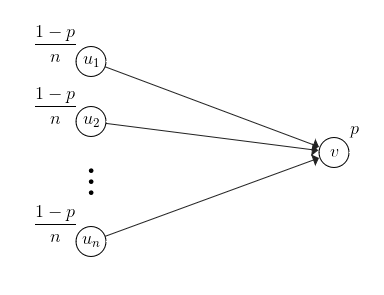
Figure 1: Graph $G$ which yields the desired lower bound.

It is easy to see that $f$ is submodular. Notice that

$$f^{+}(\bm{x})=1-p,$$

as the coefficients that maximize $\sum_{S}{a_{S}f(S)}$ subject to the constraints are $a_{\{v\}}=p$, $a_{\{u_{i}\}}=\frac{1-p}{n}$ for all $i\in\{1,\dots,n\}$ and $a_{S}=0$, for $|S|\neq 1$. In other words, $a_{\{u\}}=x_{u}$ for all $u\in V$, and $a_{S}=0$, if $|S|\neq 1$.

Next, notice that, if $R(\bm{x})\subseteq V$ is a random set, where each element $u\in V$ is sampled with probability $x_{u}$, then $f(R(\bm{x}))=1$ if and only if $v$ is not selected in $R(\bm{x})$, but at least one element of $V\setminus\{v\}$ is selected. Therefore,

$$F(\bm{x})=\mathop{\mathbb{E}}[f(R(\bm{x}))]=(1-p)\cdot\left(1-{\left(1-\frac{1-p}{n}\right)}^{n}\right),$$

which implies that

$$\frac{F(\bm{x})}{f^{+}(\bm{x})}=\frac{(1-p)\cdot\left(1-{\left(1-\frac{1-p}{n}\right)}^{n}\right)}{1-p}=1-{\left(1-\frac{1-p}{n}\right)}^{n}.$$

As $n\to\infty$, we get

$$\lim_{n\to\infty}{1-{\left(1-\frac{1-p}{n}\right)}^{n}}=1-e^{-(1-p)}.$$

We conclude that, for any $0\leq p<1$, when $x_{i}\leq p$ for all $i$,

$$F(\bm{x})\leq\left(1-e^{-(1-p)}\right)f^{+}(\bm{x}).$$

∎

B.2 Proof of Theorem 1.3

The proof of the correlation gap is via the Measured Continuous Greedy (MCG) algorithm and its analysis [22], when applied to an appropriate polytope. Earlier, we remarked that known results on the MCG algorithm [22, 2] imply that $F_{\max}(\bm{x})\geq\frac{1}{e}f^{+}(\bm{x})$. We quickly sketch the idea implicit in prior work, before we proceed. Let $f:2^{\mathcal{N}}\rightarrow\mathbb{R}_{\geq 0}$ be a non-negative submodular function and let $\bm{x}\in[0,1]^{n}$, where $n=|\mathcal{N}|$. Consider a down-closed polytope $\mathcal{P}$ defined by all points in $[0,1]^{n}$ dominated by the given point $\bm{x}$: $\mathcal{P}\coloneqq\left\{\bm{y}\in[0,1]^{n}\>\middle|\>\forall\>1\leq i\leq n,\>\>y_{i}\leq x_{i}\right\}$. Suppose we run the MCG algorithm on $\mathcal{P}$. From Lemma 8.3 of [2] for $b=1$, for any $\varepsilon>0$, the algorithm can be used to find a point $\bm{z}_{\varepsilon}\in\mathcal{P}$ such that $F(\bm{z}_{\varepsilon})\geq\left(\frac{1}{e}-\varepsilon\right)\max_{\bm{y}\in\mathcal{P}}{f^{+}(\bm{y})}\geq\left(\frac{1}{e}-\varepsilon\right)f^{+}(\bm{x})$. Since such a point $\bm{z}_{\varepsilon}\in\mathcal{P}$ exists for any $\varepsilon>0$, by the compactness of $\mathcal{P}$ and the continuity of $F$ and $f^{+}$, it follows that there exists a point $\bm{y}\in\mathcal{P}$ such that $F(\bm{y})\geq\frac{1}{e}\cdot f^{+}(\bm{x})$. Also notice that $\bm{x}\in\mathcal{P}$, and thus

$$F_{\max}(\bm{x})=\max_{\bm{z}\in\mathcal{P}}{F(\bm{z})}\geq F(\bm{y})\geq\frac{1}{e}\cdot f^{+}(\bm{x}).$$

To prove Theorem 1.3, we use the same proof outline as above, but in the algorithm’s analysis, we take advantage of the fact that $\|\bm{x}\|_{\infty}\leq p$. Theorem 1.3 generalizes Lemma 8.3 in [2], used above.

See 1.3

Proof.

Let $\bm{\hat{x}}=\operatornamewithlimits{arg\,max}_{\bm{z}\in\mathcal{P}}{f^{+}(\bm{z})}$. Recall that there exists $\bm{\alpha}\in[0,1]^{2^{\mathcal{N}}}$ such that

$$f^{+}(\bm{\hat{x}})=\sum_{S\subseteq\mathcal{N}}{\alpha_{S}f(S)},\quad\sum_{S\subseteq\mathcal{N}}{\alpha_{S}}=1\>\>\text{ and }\>\>\sum_{S\subseteq\mathcal{N}}{\alpha_{S}\mathbbm{1}_{S}}=\bm{\hat{x}}.$$

From the analysis of Measured Continuous Greedy and the fact that $\bm{x}(b)\in\mathcal{P}$, we know that, at time $b$, for all $i\in\mathcal{N}$ we have

$$x_{i}(b)\leq\min\{1-e^{-b},p\}.$$

Let $\bm{x}=\bm{x}(b)$, and, for $S\subseteq\mathcal{N}$, consider a line of direction $\bm{d}_{S}=(\bm{x}\vee\mathbbm{1}_{S})-\bm{x}=(\mathbbm{1}_{S}-\bm{x})\vee\bm{0}$. Notice that $\bm{0}\leq\bm{d}_{S}\leq\mathbbm{1}_{S}$ for all $S\subseteq\mathcal{N}$. From Section 2.3 of [11], it follows that

$$\bm{d}_{S}\cdot\nabla F(\bm{x})\geq F(\bm{x}\vee\mathbbm{1}_{S})-F(\bm{x}).$$

Since $f$ may not be monotone, $\nabla F(\bm{x})$ may have negative entries. Let $\bm{d^{\prime}}_{S}$ be a vector obtained from $\bm{d}_{S}$ as follows: $\left(\bm{d^{\prime}}_{S}\right)_{i}=\left(\bm{d}_{S}\right)_{i}$ if ${\nabla F(\bm{x})}_{i}\geq 0$, otherwise $\left(\bm{d^{\prime}}_{S}\right)_{i}=0$. We have $\bm{0}\leq\bm{d^{\prime}}_{S}\leq\bm{d}_{S}$ and,

$$\bm{d^{\prime}}_{S}\cdot\nabla F(\bm{x})\geq\max\{0,\bm{d}_{S}\cdot\nabla F(\bm{x})\}\geq\max\{0,F(\bm{x}\vee\mathbbm{1}_{S})-F(\bm{x})\}.$$

Since ${\bm{x}(b)}_{i}\leq\min\{1-e^{-b},p\}$ for all $i\in\mathcal{N}$, by Lemma III.5 of [22], we have

$$F(\bm{x}\vee\mathbbm{1}_{S})\geq\left(1-\min\{1-e^{-b},p\}\right)f(S).$$

Therefore,

$$\bm{d^{\prime}}_{S}\cdot\nabla F(\bm{x}) \geq\max\{0,(1-p)f(S)-F(\bm{x}),e^{-b}f(S)-F(\bm{x})\}$$

$$\geq\max\{1-p,e^{-b}\}f(S)-F(\bm{x}).$$

Next, let $\bm{\hat{d}}=\sum_{S\subseteq\mathcal{N}}{\alpha_{S}\bm{d^{\prime}}_{S}}$. Since $\bm{d}_{S}\leq\mathbbm{1}_{S}$ and $\bm{d^{\prime}}_{S}\leq\bm{d}_{S}$, we have $\bm{d^{\prime}}_{S}\leq\mathbbm{1}_{S}$, and thus

$$\bm{\hat{d}}=\sum_{S\subseteq\mathcal{N}}{\alpha_{S}\bm{d^{\prime}}_{S}}\leq\sum_{S\subseteq\mathcal{N}}{\alpha_{S}\mathbbm{1}_{S}}=\bm{\hat{x}}.$$

Since $\mathcal{P}$ is downward-closed and $\bm{\hat{x}}\in\mathcal{P}$, we know that $\bm{\hat{d}}\in\mathcal{P}$. Therefore, from the above and the fact that $\bm{v}_{\text{max}}=\operatornamewithlimits{arg\,max}_{\bm{v}\in\mathcal{P}}{\bm{v}\cdot\nabla F(\bm{x})}$, we have

$$\frac{\mathop{dF(\bm{x}(b))}}{\mathop{db}} =\bm{v}_{\text{max}}(\bm{x})\cdot\nabla F(\bm{x})$$

$$\geq\bm{\hat{d}}_{S}\cdot\nabla F(\bm{x})$$

$$=\sum_{S\subseteq\mathcal{N}}{\alpha_{S}\cdot\bm{d^{\prime}}_{S}\cdot\nabla F(\bm{x})}$$

$$\geq\sum_{S\subseteq\mathcal{N}}{\alpha_{S}\left(\max\{1-p,e^{-b}\}f(S)-F(\bm{x})\right)}$$

$$\geq\max\{1-p,e^{-b}\}\sum_{S\subseteq\mathcal{N}}{\alpha_{S}f(S)}-\sum_{S\subseteq\mathcal{N}}{\alpha_{S}F(\bm{x})}$$

$$\geq\max\{1-p,e^{-b}\}f^{+}(\bm{\hat{x}})-F(\bm{x}).$$

We proceed to solve the above differential inequality. For brevity, let $y=F(\bm{x})$. Then,

$$\mathop{dy}+y\mathop{db}\geq f^{+}(\bm{\hat{x}})\max\{1-p,e^{-b}\}\mathop{db}$$

$$e^{b}\mathop{dy}+ye^{b}\mathop{db}\geq f^{+}(\bm{\hat{x}})\max\{(1-p)e^{b},1\}\mathop{db}$$

$$\mathop{d\left(ye^{b}\right)}\geq f^{+}(\bm{\hat{x}})\max\{(1-p)e^{b},1\}\mathop{db}$$

$$y\geq e^{-b}f^{+}(\bm{\hat{x}})\int_{0}^{b}{\max\{(1-p)e^{u},1\}\mathop{du}}.$$ (9)

Notice that, for $0\leq u\leq\ln{\left(\frac{1}{1-p}\right)}$, we have $(1-p)e^{u}\leq 1$, while for $\ln{\left(\frac{1}{1-p}\right)}\leq u\leq 1$, we have $1\leq(1-p)e^{u}$. Therefore, for $b\leq\ln{\left(\frac{1}{1-p}\right)}$, (9) becomes

$$y\geq e^{-b}f^{+}(\bm{\hat{x}})\int_{0}^{b}{1\mathop{du}}=b\cdot e^{-b}\cdot f^{+}(\bm{\hat{x}}),$$

whereas for $b\geq\ln{\left(\frac{1}{1-p}\right)}$, (9) becomes

$$y \geq e^{-b}f^{+}(\bm{\hat{x}})\left(\int_{0}^{\ln{\left(\frac{1}{1-p}\right)}}{1\mathop{du}}+\int_{\ln{\left(\frac{1}{1-p}\right)}}^{b}{(1-p)e^{u}\mathop{du}}\right)$$

$$=\left(1-p-e^{-b}\left(1+\ln{(1-p)}\right)\right)f^{+}(\bm{\hat{x}}).$$

We conclude that

$$F(\bm{x}(b))\geq\begin{cases}b\cdot e^{-b}\cdot\max_{\bm{z}\in\mathcal{P}}{f^{+}(\bm{z})},&\text{for }0\leq b\leq\ln{\left(\frac{1}{1-p}\right)}\\ \left(1-p-e^{-b}\left(1+\ln{(1-p)}\right)\right)\cdot\max_{\bm{z}\in\mathcal{P}}{f^{+}(\bm{z})},&\text{for }\ln{\left(\frac{1}{1-p}\right)}\leq b\leq 1.\end{cases}$$

∎

Appendix C Reduction to Small Probabilities

Observation C.1 (Observation 3.1).

Let $I=(\mathcal{N},\mathcal{U},\bm{D},\bm{X},f,\mathcal{C})$ be an instance of the Submodular Prophet Inequality problem. For every fixed $\varepsilon>0$, there is a reduction of $I$ to another instance $I^{\prime}=(\mathcal{N},\mathcal{U}^{\prime},\bm{D^{\prime}},\bm{Y},g,\mathcal{C})$ of the SPI problem such that that (i) for all $e\in\mathcal{U}^{\prime}$, $\bm{D^{\prime}}(e)\leq\varepsilon$ and (ii) there exists an $\alpha$-competitive algorithm for $I$ if and only if there exists an $\alpha$-competitive algorithm for $I^{\prime}$.

Proof Sketch.

Consider the original instance $I$ and recall that each $\mathcal{D}_{i}$ is a probability distribution over $\mathcal{U}_{i}$. Our goal is to ensure that $\mathcal{D}_{i}(e)\leq\varepsilon$ for every $e\in\mathcal{U}_{i}$. Suppose there is an element $e$ such that $\mathcal{D}_{i}(e)>\varepsilon$. We obtain a new instance $I^{\prime}$ as follows. We replace $e\in\mathcal{U}_{i}$ by $h=\left\lceil 1/\varepsilon\right\rceil$ “copies” $e_{1},e_{2},\ldots,e_{h}$; let $S_{e}$ denote this set of copies. Let $\mathcal{U}^{\prime}_{i}$ be the new set of elements. We obtain a probability distribution $\mathcal{D}^{\prime}_{i}:\mathcal{U}^{\prime}_{i}\rightarrow[0,1]$ as follows. If $e^{\prime}\in\mathcal{U}_{i}$ such that $e^{\prime}\neq e$ then $\mathcal{D}^{\prime}_{i}(e^{\prime})=\mathcal{D}_{i}(e^{\prime})$ (nothing changes for $e^{\prime}$). For each copy $e_{j}$ of $e$ we set $\mathcal{D}^{\prime}_{i}(e_{j})=\mathcal{D}_{i}(e)/h$ and by our choice of $h$ we have $\mathcal{D}^{\prime}_{i}(e_{j})\leq 1/h\leq\varepsilon$, for all $e_{j}\in S_{e}$. Thus, $\sum_{j=1}^{h}\mathcal{D}^{\prime}_{i}(e_{j})=\mathcal{D}_{i}(e)$. Since we replaced $e$ by $h$ copies of it, the ground set $\mathcal{U}$ changes to $\mathcal{U}^{\prime}$ and we now define a new submodular function $g:\mathcal{U}^{\prime}\rightarrow\mathbb{R}_{+}$ that is derived from $f$. The function $g$ treats the copies of $e$ as a “single” element and hence mimics $f$. More formally, for any $A\subseteq\mathcal{U}^{\prime}$: $g(A)=f(A)$ if $A\cap S_{e}=\emptyset$, else $g(A)=f((A\setminus S_{e})\cup\{e\})$. It is easy to verify that if $f$ is non-negative and submodular, then $g$ is also non-negative and submodular, and also inherits monotonicity from $f$. Let $I^{\prime}$ be the resulting modified instance. We observe that in $I^{\prime}$, the probability of an element from $S_{e}$ being chosen is precisely equal to $\mathcal{D}_{i}(e)$ and hence the copies of $e$ act as proxies for $e$ and the submodular function $g$ ensures that every copy behaves the same as $e$ in $f$. Note that we crucially relied on the power of submodularity in this reduction. One can apply this reduction repeatedly to reduce all realization probabilities to at most $\varepsilon$. One also notices that the reduction is computationally efficient as a function of $\varepsilon$. For any fixed $\varepsilon$, the size of $I^{\prime}$ is at most $O(1/\varepsilon)$ times the size of $I$ and a value oracle for $f$ can be used to efficiently and easily obtain a value oracle for the new submodular function $g$. ∎

Appendix D Submodular Prophet Secretary

A natural question for the prophet inequality setting is whether one can obtain better prophet inequalities when the arrival order of the random variables is not chosen by the adversary but instead is chosen uniformly at random or even chosen by the algorithm. In [21], the authors introduce the prophet secretary model, combining the best of both the secretary and prophet inequality worlds. In particular, in the prophet secretary model, the arrival order of the random variables is chosen uniformly at random. There has been much work on this model and we refer to [15, 20] for several interesting results in this and related models.

We can consider the Submodular Prophet Secretary (SPS) problem as a generalization of the standard prophet secretary problem. The setting of the SPS problem is exactly the same as the setting of the SPI problem, with the only difference being that the arrival order of the random variables in the SPS problem is chosen uniformly at random instead of adversarially. We note that our results use the OCRS for the given feasibility constraint in a black-box fashion, and thus we can use better contention resolution schemes to obtain stronger bounds for the random-order setting. Specifically, in [2], the authors introduce the notion of a Random Order Contention Resolution Scheme (ROCRS), which has improved guarantees compared to the adversarial order setting. We can use an ROCRS as a black-box, instead of an OCRS, to obtain improved bounds for the SPS problem. We do not present these bounds in this version of the paper.

References

- [1] Marek Adamczyk, Maxim Sviridenko, and Justin Ward. Submodular stochastic probing on matroids. Mathematics of Operations Research, 41(3):1022–1038, 2016.
- [2] Marek Adamczyk and Michal Wlodarczyk. Random order contention resolution schemes. In 59th IEEE Annual Symposium on Foundations of Computer Science, FOCS 2018, Paris, France, October 7-9, 2018, pages 790–801, 2018.
- [3] Shipra Agrawal, Yichuan Ding, Amin Saberi, and Yinyu Ye. Price of correlations in stochastic optimization. Operations Research, 60(1):150–162, 2012. Preliminary version in Proc. of ACM-SIAM SODA 2010.
- [4] Saeed Alaei. Bayesian combinatorial auctions: Expanding single buyer mechanisms to many buyers. SIAM Journal on Computing, 43(2):930–972, 2014.
- [5] Arash Asadpour and Hamid Nazerzadeh. Maximizing stochastic monotone submodular functions. Management Science, 62(8):2374–2391, 2016.
- [6] Sepehr Assadi, Thomas Kesselheim, and Sahil Singla. Improved truthful mechanisms for subadditive combinatorial auctions: Breaking the logarithmic barrier. In Proceedings of the 2021 ACM-SIAM Symposium on Discrete Algorithms (SODA), pages 653–661. SIAM, 2021.
- [7] Domagoj Bradac, Sahil Singla, and Goran Zuzic. (Near) Optimal Adaptivity Gaps for Stochastic Multi-Value Probing. In Dimitris Achlioptas and László A. Végh, editors, Approximation, Randomization, and Combinatorial Optimization. Algorithms and Techniques (APPROX/RANDOM 2019), volume 145 of Leibniz International Proceedings in Informatics (LIPIcs), pages 49:1–49:21, Dagstuhl, Germany, 2019. Schloss Dagstuhl–Leibniz-Zentrum fuer Informatik.
- [8] Niv Buchbinder and Moran Feldman. Submodular functions maximization problems. In Teofilo F Gonzalez, editor, Handbook of Approximation Algorithms and Metaheuristics: Methologies and Traditional Applications, Volume 1. CRC Press, 2nd edition, 2018.
- [9] Niv Buchbinder, Moran Feldman, Joseph (Seffi) Naor, and Roy Schwartz. Submodular maximization with cardinality constraints. In Proceedings of the Twenty-fifth Annual ACM-SIAM Symposium on Discrete Algorithms, SODA ’14, pages 1433–1452, Philadelphia, PA, USA, 2014. Society for Industrial and Applied Mathematics.
- [10] G Calinescu, C Chekuri, M Pal, and J Vondrak. Maximizing a submodular function subject to a matroid constraint. In the Proceedings of the Conference on Integer Programming and Combinatorial Optimization (IPCO), 2007.
- [11] Gruia Calinescu, Chandra Chekuri, Martin Pál, and Jan Vondrák. Maximizing a monotone submodular function subject to a matroid constraint. SIAM Journal on Computing, 40(6):1740–1766, 2011.
- [12] Shuchi Chawla, Jason D Hartline, David L Malec, and Balasubramanian Sivan. Multi-parameter mechanism design and sequential posted pricing. In Proceedings of the forty-second ACM symposium on Theory of computing, pages 311–320, 2010.
- [13] Shuchi Chawla and Balasubramanian Sivan. Bayesian algorithmic mechanism design. SIGecom Exch., 13(1):5–49, November 2014.
- [14] Chandra Chekuri, Jan Vondrák, and Rico Zenklusen. Submodular function maximization via the multilinear relaxation and contention resolution schemes. In Proceedings of the Forty-third Annual ACM Symposium on Theory of Computing, STOC ’11, pages 783–792, New York, NY, USA, 2011. ACM.
- [15] José Correa, Patricio Foncea, Ruben Hoeksma, Tim Oosterwijk, and Tjark Vredeveld. Recent developments in prophet inequalities. ACM SIGecom Exchanges, 17(1):61–70, 2019.
- [16] Michael Dinitz. Recent advances on the matroid secretary problem. ACM SIGACT News, 44(2):126–142, 2013.
- [17] Paul Dütting, Thomas Kesselheim, and Brendan Lucier. An prophet inequality for subadditive combinatorial auctions. ACM SIGecom Exchanges, 18(2):32–37, 2020.
- [18] E. B. Dynkin. The optimum choice of the instant for stopping a Markov process. Soviet Math. Dokl, 4, 1963.
- [19] Paul Dütting, Michal Feldman, Thomas Kesselheim, and Brendan Lucier. Prophet inequalities made easy: Stochastic optimization by pricing nonstochastic inputs. SIAM Journal on Computing, 49(3):540–582, 2020.
- [20] Soheil Ehsani, MohammadTaghi Hajiaghayi, Thomas Kesselheim, and Sahil Singla. Prophet secretary for combinatorial auctions and matroids. In Proceedings of the Twenty-Ninth Annual ACM-SIAM Symposium on Discrete Algorithms, SODA ’18, page 700–714, USA, 2018. Society for Industrial and Applied Mathematics.
- [21] Hossein Esfandiari, MohammadTaghi Hajiaghayi, Vahid Liaghat, and Morteza Monemizadeh. Prophet secretary. CoRR, abs/1507.01155, 2015.
- [22] Moran Feldman, Joseph (Seffi) Naor, and Roy Schwartz. A unified continuous greedy algorithm for submodular maximization. In Proceedings of the 2011 IEEE 52Nd Annual Symposium on Foundations of Computer Science, FOCS ’11, pages 570–579, Washington, DC, USA, 2011. IEEE Computer Society.
- [23] Moran Feldman, Ola Svensson, and Rico Zenklusen. Online contention resolution schemes. In Proceedings of the Twenty-seventh Annual ACM-SIAM Symposium on Discrete Algorithms, SODA ’16, pages 1014–1033, Philadelphia, PA, USA, 2016. Society for Industrial and Applied Mathematics.
- [24] Moran Feldman and Rico Zenklusen. The submodular secretary problem goes linear. SIAM Journal on Computing, 47(2):330–366, 2018.
- [25] Anupam Gupta and Viswanath Nagarajan. A stochastic probing problem with applications. In Michel Goemans and José Correa, editors, Integer Programming and Combinatorial Optimization, pages 205–216, Berlin, Heidelberg, 2013. Springer Berlin Heidelberg.
- [26] Anupam Gupta, Viswanath Nagarajan, and Sahil Singla. Adaptivity Gaps for Stochastic Probing: Submodular and XOS Functions, pages 1688–1702.
- [27] Anupam Gupta, Viswanath Nagarajan, and Sahil Singla. Algorithms and Adaptivity Gaps for Stochastic Probing, pages 1731–1747.
- [28] Anupam Gupta and Sahil Singla. Random-order models, 2020. https://arxiv.org/abs/2002.12159.
- [29] Mohammad Taghi Hajiaghayi, Robert Kleinberg, and Tuomas Sandholm. Automated online mechanism design and prophet inequalities. In Proceedings of the 22Nd National Conference on Artificial Intelligence - Volume 1, AAAI’07, pages 58–65. AAAI Press, 2007.
- [30] Jason D. Hartline. Bayesian mechanism design. Foundations and Trends® in Theoretical Computer Science, 8(3):143–263, 2013.
- [31] Theodore P Hill and Robert P Kertz. A survey of prophet inequalities in optimal stopping theory. Contemp. Math, 125:191–207, 1992.
- [32] Sanchit Kalhan. A study on matroid prophet inequalities. Senior thesis, University of Illinois at Urbana-Champaign, May 2016.
- [33] Robert Kleinberg and Seth Matthew Weinberg. Matroid prophet inequalities. In Proceedings of the forty-fourth annual ACM symposium on Theory of computing, pages 123–136, 2012.
- [34] Ulrich Krengel and Louis Sucheston. Semiamarts and finite values. Bull. Amer. Math. Soc., 83(4):745–747, 07 1977.
- [35] Brendan Lucier. An economic view of prophet inequalities. SIGecom Exch., 16(1):24–47, September 2017.
- [36] Aviad Rubinstein. Beyond Matroids: Secretary Problem and Prophet Inequality with General Constraints, page 324–332. Association for Computing Machinery, New York, NY, USA, 2016.
- [37] Aviad Rubinstein and Sahil Singla. Combinatorial prophet inequalities. In Proceedings of the Twenty-Eighth Annual ACM-SIAM Symposium on Discrete Algorithms, pages 1671–1687. SIAM, 2017. Longer ArXiv version is at http://arxiv.org/abs/1611.00665.
- [38] Sahil Singla. Combinatorial Optimization Under Uncertainty: Probing and Stopping-Time Algorithms. PhD thesis, CMU, 2018. http://reports-archive.adm.cs.cmu.edu/anon/2018/CMU-CS-18-111.pdf.
- [39] Jan Vondrák. Submodularity in combinatorial optimization. PhD thesis, Univerzita Karlova, Matematicko-fyzikální fakulta, 2007.
- [40] Qiqi Yan. Mechanism design via correlation gap. In Dana Randall, editor, Proceedings of the Twenty-Second Annual ACM-SIAM Symposium on Discrete Algorithms, SODA 2011, San Francisco, California, USA, January 23-25, 2011, pages 710–719. SIAM, 2011.