Supplementary Material for Causal Structural Learning Via Local Graphs

1 Additional results

Definition 1 (PAG).

Let $G=(X\cup L\cup Z,E)$ be a DAG, and $H$ be a simple graph with vertex set $X$ and edges of the type $\to$, $\mathrlap{\multimapinv}\to$, $\multimapboth$, $\leftrightarrow$, $-$, or $\multimapinv$. Then $H$ is a PAG representing $G$ if and only if the following four conditions hold:

1. The absence of an edge between two vertices $i$ and $j$ in $H$ implies that there exists a subset $Y\subseteq X\setminus\{i,j\}$ such that $i$ and $j$ are $m$-separated given $(Y\cup Z)$.

2. The presence of an edge between two vertices $i$ and $j$ in $H$ implies that $i$ and $j$ are $m$-connected given $(Y\cup Z)$ for all subsets $Y\subseteq X\setminus\{i,j\}$.

3. If an edge between $i$ and $j$ in $H$ has an arrowhead at $j$, then $j\notin\mathrm{an}(G,i\cup Z)$.

4. If an edge between $i$ and $j$ in $H$ has a tail at $j$, then $j\in\mathrm{an}(G,i\cup Z)$.

2 Additional Proofs

Proof of Lemma 3.

Figure 1: Local graph configurations with $\eta=3$ and $|\mathrm{ne}(G_{\gamma}(i,j),i)|=1$. A separator (not necessarily minimal) is marked with shade. Marked edge represents the pattern of $G_{\gamma}(i,j)$, while absence of an edge represents the absence pattern of $G_{\gamma}(i,j)$. Ellipses between nodes means this edge is allowed to occur in $G_{\gamma}(i,j)$, as long as it agrees with the MAG property and local-path property. The square shape represents a node with no outgoing edge (except the marked ones). The diamond shape represents a node that controls whether the separator is minimum — if this node is not ancestor of $j$, then smaller separator exists.

Figure 2: Local graph configurations with $\eta=3$ and $|\mathrm{ne}(G_{\gamma}(i,j),i)|=2$. (continues in Figure 3). A separator (not necessarily minimal) is marked with shade. Marked edge represents the pattern of $G_{\gamma}(i,j)$, while absence of an edge represents the absence pattern of $G_{\gamma}(i,j)$. Ellipses between nodes means this edge is allowed to occur in $G_{\gamma}(i,j)$, as long as it agrees with the MAG property and local-path property. The square shape represents a node with no outgoing edge (except the marked ones). The diamond shape represents a node that controls whether the separator is minimum — if this node is not ancestor of $j$, then smaller separator exists.

Figure 3: Local graph configurations with $\eta=3$ and $|\mathrm{ne}(G_{\gamma}(i,j),i)|=2$. A separator (not necessarily minimal) is marked with shade. Marked edge represents the pattern of $G_{\gamma}(i,j)$, while absence of an edge represents the absence pattern of $G_{\gamma}(i,j)$. Ellipses between nodes means this edge is allowed to occur in $G_{\gamma}(i,j)$, as long as it agrees with the MAG property and local-path property. The square shape represents a node with no outgoing edge (except the marked ones). The diamond shape represents a node that controls whether the separator is minimum — if this node is not ancestor of $j$, then smaller separator exists.

1. $|\mathrm{ne}(G_{\gamma}(i,j),i)|=1$. (Figure 1) Denote the only neighbor as $u$. If $i\to u$ or $i\leftrightarrow u$ but $u\notin\mathrm{an}(G_{\gamma}(i,j),j)$, then $S_{\gamma}(i,j)=\emptyset$. If $i\leftarrow u$ or $i-u$, then $S_{\gamma}(i,j)=\{u\}$. If $i\leftrightarrow u$ and $u\in\mathrm{an}(G_{\gamma}(i,j),j)$, then there must be an edge $u\to w$ and $w\in\mathrm{an}(G_{\gamma}(i,j),j)$. If $\mathrm{ne}(G_{\gamma}(i,j),u)=\{i,w\}$ then $S_{\gamma}(i,j)=\{u\}$. Now discuss cases with additional neighbors.

   1. If $\mathrm{ne}(G_{\gamma}(i,j),u)=\{i,w,v\}$, we have $S_{\gamma}(i,j)=\{u\}$ if $u\to v$ or $u\leftrightarrow v$ but $v\notin\mathrm{an}(G_{\gamma}(i,j),j)$; also $S_{\gamma}(i,j)=\{u,v\}$ if $u\leftarrow v$ or $u\leftrightarrow v$ and $v\in\mathrm{an}(G_{\gamma}(i,j),j)$ and $v$ has exactly one neighbor other than $u$ (it is allowed to be $w$). If $v$ has 2 neighbors other than $u$, and neither is child of $v$, then $v\notin\mathrm{an}(G_{\gamma}(i,j),j)$, which is covered in the previous case. Now suppose $v\to x$ and there is also an edge $v{\setstackEOL{}\setstackgap{L}{0pt}\Longstack[c]{$\star-$\kern 6.45831pt$-\star$}}y$, in which case $|e^{b}_{2}|+|e^{m}_{2}|=3$. We have $S_{\gamma}(i,j)=\{u,v,y\}$ if $v\leftarrow y$ or $v\leftrightarrow y$ and $y\in\mathrm{an}(G_{\gamma}(i,j),j)$, and otherwise $S_{\gamma}(i,j)=\{u,v\}$.

   2. If $\mathrm{ne}(G_{\gamma}(i,j),u)=\{i,w,v,x\}$, then $|e^{b}_{2}|=3$ and $S_{\gamma}(i,j)\subseteq\{u,v,x\}$.

2. $|\mathrm{ne}(G_{\gamma}(i,j),i)|=2$. Denote the neighbors as $u$ and $v$. We discuss the direction of the two edges $i{\setstackEOL{}\setstackgap{L}{0pt}\Longstack[c]{$\star-$\kern 6.45831pt$-\star$}}u$ and $i{\setstackEOL{}\setstackgap{L}{0pt}\Longstack[c]{$\star-$\kern 6.45831pt$-\star$}}v$. If the directions are $(\to,\to)$ , then $S_{\gamma}(i,j)=\emptyset$. If $(\leftarrow,\to)$, then $S_{\gamma}(i,j)=\{u\}$. If $(\leftarrow,\leftarrow)$ or $(-,\leftarrow)$ or $(-,-)$, then $S_{\gamma}(i,j)=\{u,v\}$.

   1. If $(\leftrightarrow,\leftarrow)$, then we need to discuss neighbors of $u$, too. If $u\in\mathrm{adj}(G_{\gamma}(i,j),v)$, then $u{\setstackEOL{}\setstackgap{L}{0pt}\Longstack[c]{$\star-$\kern 6.45831pt$-\star$}}v$ is a merging edge, and by Fact 2, $u$ and $v$ have in total no more than 2 bearing edges of order 2. If $u$ is not ancestral to $i$ or $j$, then $S_{\gamma}(i,j)=\{v\}$. The case of $u\notin\mathrm{an}(G_{\gamma}(i,j),\{i,j\})$ is trivial. If $u\in\mathrm{an}(G_{\gamma}(i,j),\{i,j\})$, then $u$ has at least one outgoing edge. If the outgoing edge is $u\to v$ (second row of Figure 2), there are two sub-cases. If $v$ has an bearing edge of order 2, then $u$ has only one other neighbor, call it $x$, and we condition on $x$ if and only if $u\leftarrow x$ or $u\leftrightarrow x$ and $x\in\mathrm{an}(G_{\gamma}(i,j),j)$. If $v$ has no bearing edge, then $u$ can have at most 2 other neighbors. However, these bearing edges must not have arrow at $u$, due to the inducing path interpretation of MAG. Therefore we do not need to condition on these additional neighbors.

      If the outgoing edge is not $u\to v$ (third row of Figure 2), then there is some edge $u\to w$. If $v$ has an bearing edge of order 2, then $u$ no other neighbor than $\{i,u,w\}$. If $v$ has no bearing edge, then $u$ could have one additional neighbor, call it $x$, and we condition on $x$ if and only if $u\leftarrow x$ or $u\leftrightarrow x$ and $x\in\mathrm{an}(G_{\gamma}(i,j),j)$.

      If $u\notin\mathrm{adj}(G_{\gamma}(i,j),v)$ (fourth row of Figure 2), then $u$ has at most two additional neighbors. If none of them are child of $u$, then $u\notin\mathrm{an}(G_{\gamma}(i,j),\{i,j\})$ and $S_{\gamma}(i,j)=\{v\}$; If $u\to w$, $u{\setstackEOL{}\setstackgap{L}{0pt}\Longstack[c]{$\star-$\kern 6.45831pt$-\star$}}x$ then we condition on $x$ if and only if $u\leftarrow x$ or $u\leftrightarrow x$ and $x\in\mathrm{an}(G_{\gamma}(i,j),j)$.

   2. if $(\leftrightarrow,\to)$, the situations are simpler since we never condition on $v$. Since $v$ must have either a bearing edge or a merging edge, $u$ can have at most 2 bearing edges. If $u\in\mathrm{an}(G_{\gamma}(i,j),j)$, then one of the edges is $u\to w$. As for the other one, $u{\setstackEOL{}\setstackgap{L}{0pt}\Longstack[c]{$\star-$\kern 6.45831pt$-\star$}}x$, we condition on $x$ if and only if $u\leftarrow x$ or $u\leftrightarrow x$ and $x\in\mathrm{an}(G_{\gamma}(i,j),j)$.

   3. If $(\leftrightarrow,\leftrightarrow)$: If neither of $u$ and $v$ are ancestral to $j$, then $S_{\gamma}(i,j)=\emptyset$. If both are ancestral to $j$ (row 2-3 and first 2 figures of row 4 in Figure 3), then they each has a outgoing edge. Then by Fact 2, there is at most one other bearing edge. WLOG, suppose $u$ has $u\to w$ and $u{\setstackEOL{}\setstackgap{L}{0pt}\Longstack[c]{$\star-$\kern 6.45831pt$-\star$}}x$. Then $S_{\gamma}(i,j)=\{u,v,x\}$ if $x\in\mathrm{an}(G_{\gamma}(i,j),\{u,j\})$ and otherwise $S_{\gamma}(i,j)=\{u,v\}$. If $u$ is ancestral to $j$ and $v$ is not, then still $u$ has one outgoing edge and at most one other edge. Then $S_{\gamma}(i,j)=\{u,x\}$ if $x\in\mathrm{an}(G_{\gamma}(i,j),\{u,j\})$ and otherwise $S_{\gamma}(i,j)=\{u\}$.

3. $|\mathrm{ne}(G_{\gamma}(i,j),i)|=3$. Denote the three neighbors of $i$ as $u,v,w$. By Fact 2, they each has at most one bearing edge. Therefore we do not need to look further, and $S_{\gamma}(i,j)\subseteq\{u,v,w\}$.

∎

The following proof is similar to Lemma 2 of Sondhi and Shojaie, (2019) with slight modification, we show the proof here for completeness.

Proof of Lemma 5.7.

We write

$$\Sigma =(I-B)^{-1}\Omega(I-B)^{-\top}$$

$$=\left(\sum_{r=0}^{p-1}B^{r}\right)\Omega\left(\sum_{r=0}^{p-1}B^{r}\right)^{\top}$$

$$=\left(\sum_{r=0}^{\gamma}B^{r}+\sum_{r=\gamma+1}^{p-1}B^{r}\right)\Omega\left(\sum_{r=0}^{\gamma}B^{r}+\sum_{r=\gamma+1}^{p-1}B^{r}\right)^{\top}$$

Denote $\Lambda_{H}=\sum_{r=0}^{\gamma}B^{r}$ and $R_{\gamma}=\sum_{r=\gamma+1}^{\infty}B^{r}=\sum_{r=\gamma+1}^{p-1}B^{r}$. By the directed $\beta$-summability assumption, we have $\lVert{\Lambda_{H}}\rVert\leq\frac{1-\beta^{\gamma+1}}{1-\beta}$ and $\lVert{R_{\gamma}}\rVert\leq\frac{\beta^{\gamma+1}-\beta^{p}}{1-\beta}$. Now we can bound the difference between $\Sigma$ and the local approximation version $\Sigma_{H}:=\Lambda_{H}\Omega\Lambda_{H}^{\top}$, which only contains paths no longer than $\gamma$.

$$\lVert{\Sigma-\Sigma_{H}}\rVert =\lVert{\Lambda_{H}\Omega R_{\gamma}^{\top}+R_{\gamma}\Omega\Lambda_{H}^{\top}+R_{\gamma}\Omega R_{\gamma}^{\top}}\rVert$$

$$\leq\lVert{\Omega}\rVert\left(2\lVert{\Lambda_{H}}\rVert\lVert{R_{\gamma}}\rVert+\lVert{R_{\gamma}}\rVert^{2}\right)$$

$$\leq\lVert{\Omega}\rVert\left(2\frac{(1-\beta^{\gamma+1})\beta^{\gamma+1}}{(1-\beta)^{2}}+\frac{\beta^{2\gamma+2}}{(1-\beta)^{2}}\right)$$

$$=\lVert{\Omega}\rVert\frac{\beta^{\gamma+1}(2-\beta^{\gamma+1})}{(1-\beta)^{2}}$$

We write $\gamma*=\log(\beta)^{-1}\left(\log M-\log 2-\log\lVert{\Omega}\rVert-\log(\eta+2)-\log(1+3/\lambda)\right)-1$. We invoke the error propagation lemma from Harris and Drton, (2013). For any non-adjacent pair $(i,j)$ and a set $S\subseteq V\setminus\{i,j\}$ with $|S|\leq\eta$, whenever $\gamma\geq\gamma^{*}$, it holds that

$$|\rho(i,j|S)-\rho_{H}(i,j|S)|\leq\lambda$$

where $\rho_{H}$ is the partial correlation obtained from $\Sigma_{H}$. Since $\Sigma_{H}$ only composes of short paths, $\rho_{H}(i,j|S_{\gamma})=0$ for every local-graph separator $S_{\gamma}$. Therefore $|\rho(i,j|S_{\gamma})|<\lambda$. ∎

3 Treks

In this section we provide an algebraic explanation of Assumption 5. In particular, we review the trek representation of partial correlation in linear SEM. The representation clarifies that conditional dependence in a linear SEM is tied to existence of paths/treks in the graph underlying the model. This allows us to argue that conditional dependence is typically induced by short versus long treks, which in turn provides the basis for exploiting small local separators in our algorithms.

To simplify the discussion, we present the following results assuming there is no selection variables in the graph. Let $G$ be a mixed graph without undirected edges. We define a trek from node $i$ to $j$ as a tuple $\tau=(P_{L},P_{M},P_{R})$, where $P_{L}$ is a directed path from some node $s$ to $i$, and $P_{R}$ is a directed path from some node $t$ to $j$, and $P_{M}$ is either one bidirected edge $s\leftrightarrow t$ or the empty set when $s=t$. We define the trek monomial as $m_{\tau}=\beta^{L}\omega_{s,t}\beta^{R}$, where $\beta^{L}=\prod_{k\to l\in P_{L}}\beta_{kl}$ and $\beta^{R}=\prod_{k\to l\in P_{R}}\beta_{kl}$. Moreover, for sets $C$ and $D$ with $|C|=|D|=k$, we define a trek system $T$ from $C$ to $D$ as a set of $k$ treks whose initial nodes exhaust $C$ and final nodes exhaust $D$. With abuse of notation we write $T$ as a tuple of collections of paths $(P_{L},P_{M},P_{R})$, and define the trek system monomial as the product of trek monomials in the system, i.e., $m_{T}=\prod_{\tau\in T}m_{\tau}$. Each trek system determines a permutation of the initial and final nodes, which we call the sign of the system. Let $\mathcal{T}(C,D)$ denote the collection of all trek systems from $C$ to $D$. By the Cauchy–Binet determinant expansion, we have,

$$\det\Sigma(C,D) =\sum_{R,S\subset V,|R|=|S|=k}\det\left((I-B)^{-\top}\right)_{C,R}\det\Omega_{R,S}\det\left((I-B)^{-1}\right)_{S,D}$$ (1)

$$=\sum_{T\in\mathcal{T}(C,D)}\operatorname{sign}(T)m_{T}.$$ (2)

We say a trek system $T$ has sided intersection if two paths in $P_{L}$, $P_{R}$, or $P_{M}$ have shared nodes. If $T$ is a trek system between $C$ and $D$ with sided intersections, then its weight $m_{T}$ is cancelled in the summation in (2), (for a proof, see Sullivant et al.,, 2010). In other words, the summation in (2) only needs to run over trek systems without sided intersections. Consequently, $\det\left(\Sigma(i\cup S,j\cup S)\right)=0$ if and only if every system of treks from $i\cup S$ to $j\cup S$ has a sided intersection. The later condition is also called $t$-separation. For Gaussian SEMs, in which conditional independence is characterized by zero partial correlation, this means $W_{i}\mathchoice{\mathrel{\hbox to0.0pt{$\displaystyle\perp$\hss}\mkern 3.0mu{\displaystyle\perp}}}{\mathrel{\hbox to0.0pt{$\textstyle\perp$\hss}\mkern 3.0mu{\textstyle\perp}}}{\mathrel{\hbox to0.0pt{$\scriptstyle\perp$\hss}\mkern 3.0mu{\scriptstyle\perp}}}{\mathrel{\hbox to0.0pt{$\scriptscriptstyle\perp$\hss}\mkern 3.0mu{\scriptscriptstyle\perp}}}W_{j}|W_{S}$ if and only if $\sum_{T\in\mathcal{T}(i\cup S,j\cup S)}\operatorname{sign}(T)m_{T}=0$.

We will show next that Assumption 5 can be expressed as a condition on trek weights. Let $G=(V,E)$ be a MAG. For non-adjacent nodes $i,j\in V$, and $S\subseteq V(G_{\gamma})\setminus\{i,j\}$, we denote $\mathcal{T}_{\gamma}(i,j,S)$ as the collection of trek systems from $i\cup S$ to $j\cup S$ in $G_{\gamma}(i,j)$, and $\mathcal{T}^{C}_{\gamma}(i,j,S):=\mathcal{T}(i\cup S,j\cup S)\setminus\mathcal{T}^{C}_{\gamma}(i,j,S)$. By our definition, $\mathcal{T}^{C}_{\gamma}(i,j,S)$ only contains treks that goes through a node outside $G_{\gamma}(i,j)$.

Lemma 1.

Let $G$ be a MAG. Under Assumption 3, if there exists $\beta\in(0,1)$ such that

$$\max_{i\notin\mathrm{adj}(G,j)}\min_{S_{\gamma}\in\mathcal{S}_{\eta,\gamma}(i,j)}\left|\sum_{T\in\mathcal{T}^{C}_{\gamma}(i,j,S_{\gamma})}\operatorname{sign}(T)m_{T}\right|=O(\beta^{\gamma}),$$

where $\mathcal{S}_{\eta,\gamma}(i,j)$ is the collection of $\gamma$-local-graph separators of size at most $\eta$, then Assumption 5 holds.

Proof.

By Definition 4, if a set $S_{\gamma}$ is a $\gamma$-local-separator of $(i,j)$, then it is a separator of $i$ and $j$ in $G_{\gamma}(i,j)$, so all trek systems between $i\cup S_{\gamma}$ and $j\cup S_{\gamma}$ have sided intersections in $G_{\gamma}(i,j)$, and hence also in $G$. Following Draisma et al., (2013), we only need to take summation over trek systems without sided intersection in $G$. Therefore,

$$\sum_{T\in\mathcal{T}(i,j,S_{\gamma})}\operatorname{sign}(T)m_{T} =\sum_{T\in\mathcal{T}_{\gamma}(i,j,S_{\gamma})}\operatorname{sign}(T)m_{T}+\sum_{T\in\mathcal{T}^{C}_{\gamma}(i,j,S_{\gamma})}\operatorname{sign}(T)m_{T}$$

$$=\sum_{T\in\mathcal{T}^{C}_{\gamma}(i,j,S_{\gamma})}\operatorname{sign}(T)m_{T}.$$

Now denote $\Sigma(i,j|S_{\gamma})$ as the $(i,j)$-th entry of the conditional variance matrix given $S_{\gamma}$. We have

$$\rho(i,j|S_{\gamma}) =\frac{\Sigma(i,j|S_{\gamma})}{\sqrt{\Sigma(i,i|S_{\gamma})\Sigma(j,j|S_{\gamma})}}=\frac{\sum_{T\in\mathcal{T}(i,j,S_{\gamma})}\operatorname{sign}(T)m_{T}}{\det(\Sigma(S_{\gamma},S_{\gamma}))}\frac{1}{\sqrt{\Sigma(i,i|S_{\gamma})\Sigma(j,j|S_{\gamma})}}.$$

By the fact that $\Sigma(j,j|S_{\gamma})\geq\Sigma(j,j|V\setminus\{j\})=1/\omega_{jj}$, and $\det(\Sigma(S_{\gamma},S_{\gamma}))\geq M^{-\eta}$ under Assumption 3, we have $|\rho(i,j|S_{\gamma})|=O(\beta^{\gamma}).$ ∎

4 Choice of $\gamma$

Recall the simulation study in Section 6. We randomly generate Erdős-Renyi graphs and power-law graphs with $p=|V|=200$ nodes and average node degree 2. Edge weights are drawn uniformly from $\pm[.1,1]$, and $n=100$ observations are generated by the rmvDAG function. We randomly choose $q=0.2p$ nodes as latent variables, and the rest as observed. We include no selection variables. We run lFCI with $\gamma=\{2,3,4,5,6,7,8,p/2,p-1\}$, and $\alpha=\{10^{-15,},10^{-9},10^{-8},10^{-7},\cdot 10^{-6},10^{-3},\cdot 10^{-5},10^{-4},10^{-3},10^{-2}\}$. We repeat the experiment 100 times for each $\alpha$, and compare the true positive and false positive discoveries of the skeleton of the true PAG.

Figure 4 suggests that as long as $\gamma$ is large enough, the algorithm yields almost identical outputs. The only exception is the case of power-law graph with $\gamma=2$, in which the algorithm appears to be too aggressive, and the performance is sub-par on a part of the pROC curve. We also point out that in the “many false positive” part of the curves (i.e., to the right end), methods with smaller $\gamma$ tends to perform better, since they perform fewer tests. However, that region is only relevant for “discovery”. In general, we recommend using $\gamma=O(\log|V|)$.

5 Simulations with standardized normal coefficients

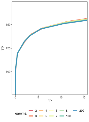
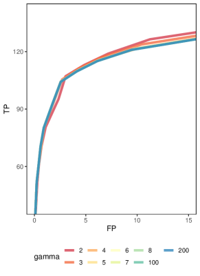
Figure 4: pROC curves of Algorithm 1 with different choices of $\gamma$ performed on ER graphs (left) and power-law graphs (right).

In this section, we aim to provide evidence that Assumption 5 is satisfied in many common large networks when data is standardized. The fact that in many common scenarios the SEM corresponding to the standardized data has almost all coefficients less than 1 is demonstrated in a simulation study in Appendix B of Sondhi and Shojaie, (2019). We further conjecture that the sum of long trek weights are also minimal, by showing the covariance matrix is well approximated using only short treks. For this purpose, we generate a random ER or power-law graph and draw edge weights from either a uniform distribution on $(-10,10)$ or a normal distribution with mean 0 and standard deviation $3$. We intentionally choose wide ranges for the coefficient to allow large fluctuation in the network. Then a SEM in the form of (2) is constructed with this weighted adjacency matrix $B$ and random error variance $\Omega$, where $\Omega$ is a diagonal matrix with diagonal entries drawn from a uniform distribution on $(1,2)$. We denote $\Sigma=(I-B)^{-1}\Omega(I-B)^{-\top}$ and $\widetilde{\Sigma}$ as its standardized version, where $\widetilde{\Sigma}_{ij}=\Sigma_{ij}/\sqrt{\Sigma_{ii}\Sigma_{jj}}$ for each $(i,j)$-entry. The standardized data can be seem as drawn from another SEM corresponding to the same graph $G$, but with different set of parameters $(\widetilde{B},\widetilde{\Omega})$, which satisfies $\widetilde{\Sigma}=(I-\widetilde{B})^{-1}\widetilde{\Omega}(I-\widetilde{B})^{-\top}$. We compute the maximal entry-wise difference between $\widetilde{\Sigma}$ and its short-trek approximation $\widetilde{\Sigma}_{\gamma}=(\sum_{k=0}^{\gamma}\widetilde{B})\widetilde{\Omega}(\sum_{k=0}^{\gamma}\widetilde{B})^{\top}$. We define $d_{\gamma}:=\max_{i,j}(|\widetilde{\Sigma}-\widetilde{\Sigma}_{\gamma}{}|_{i,j})$ and report the smallest $\gamma$ such that $d_{\gamma}\leq 10^{-4}$ over 100 iterations. We use the quantity $d_{\gamma}$ as a surrogate to check Assumption 5 because we have shown in the proof of Lemma 5.7 that $\lVert{\widetilde{\Sigma}-\widetilde{\Sigma}_{\gamma}}\rVert=O(\beta^{\gamma})$ is a sufficient condition of Assumption 5.

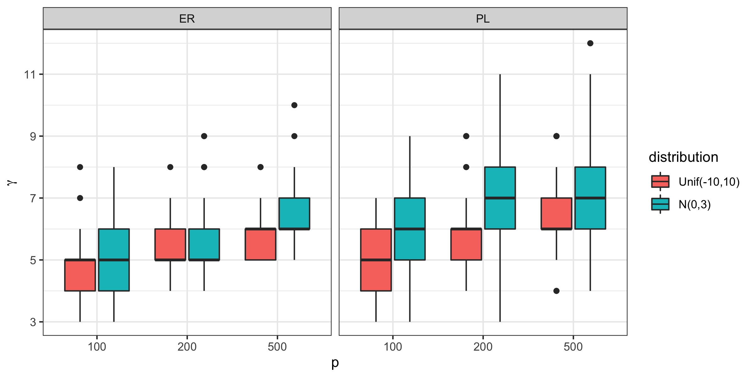
Figure 5: Values of $\min\{\gamma:d_{\gamma}\leq 10^{-4}\}$ for various settings of ER and power-law graphs, with edge weights drawn from either Uniform $(-10,10)$ or $N(0,3^{2})$, and $n=100,200,500$. The minimal $\gamma$ values scale with $\log p$.

Figure 5 demonstrates $d_{\gamma}$ is indeed very small in most settings with $\gamma\approx\log p$. The results suggest that Assumption 5 is indeed plausible for standardized data.

6 Simulations with local moral graphs

In this section we demonstrate that with large enough $\gamma$, the $\gamma$-local moral graphs usually coincide with moral graphs. Following the simulation settings in Section 6, in the numerical study below, we generate random DAGs with $p\in\{100,200,500\}$ nodes and average node degree $2$. Similarly, we also use $\gamma=5,6,7$ for $p=100,200,500$ and randomly choose $q=0.2p$ nodes as latent nodes, and compute the skeleton of the MAG over the observed ones. We do not introduce selection variables, simply because undirected edges do not contribute to the difference between local and non-local Markov blankets.

We compute the moral graph and $\gamma$-local moral graph for each MAG over 200 simulation iterations, and report the proportion of cases when local moral graph is different from the moral graph. The results are reported in Table 1. We see for the choice of $\gamma$ used in our simulations, almost all local moral graphs are identical to the moral graphs. This is especially likely to be true for power-law graphs, since they tends to have smaller diameter.

	Erdős-Renyi	Power Law	Watts-Strogatz
$p=100$, $\gamma=5$	0.99	1.00	0.96
$p=200$, $\gamma=6$	0.99	1.00	0.97
$p=500$, $\gamma=7$	0.99	1.00	0.97

Table 1: Proportion of random graphs (out of 200 iterations) with $\gamma$-local moral graph equal to moral graph.

7 Search Pools

The graph in Figure 6 is an example in which lFCI may needs to perform more conditional independence tests than FCI.

Figure 6: No edge is removed at level 0. At level 1, if the edge $(x,y)$ is checked after removing $(x,2)$ and $(2,y)$, then FCI performs less CI tests than lFCI (with $\gamma=5$), because the node $2$ is local to $x$ and $y$ but not in their neighborhoods.

References

• Ali et al., (2009) Ali, R. A., Richardson, T. S., and Spirtes, P. (2009). Markov equivalence for ancestral graphs. Ann. Statist., 37(5B):2808–2837.
• Anandkumar et al., (2011) Anandkumar, A., Hassidim, A., and Kelner, J. (2011). Topology discovery of sparse random graphs with few participants. SIGMETRICS Perform. Eval. Rev., 39(1):253–264.
• (3) Anandkumar, A., Tan, V. Y. F., Huang, F., and Willsky, A. S. (2012a). High-dimensional Gaussian graphical model selection: walk summability and local separation criterion. J. Mach. Learn. Res., 13:2293–2337.
• (4) Anandkumar, A., Tan, V. Y. F., Huang, F., and Willsky, A. S. (2012b). High-dimensional structure estimation in Ising models: local separation criterion. Ann. Statist., 40(3):1346–1375.
• Bollobás and Béla, (2001) Bollobás, B. and Béla, B. (2001). Random Graphs. Cambridge Studies in Advanced Mathematics. Cambridge University Press.
• Cancer-Genome-Atlas-Research-Network, (2012) Cancer-Genome-Atlas-Research-Network (2012). Comprehensive genomic characterization of squamous cell lung cancers. Nature, 489(7417):519–525.
• Chen and Sharp, (2004) Chen, H. and Sharp, B. M. (2004). Content-rich biological network constructed by mining pubmed abstracts. BMC Bioinformatics, 5:147 – 147.
• Chung and Lu, (2006) Chung, F. and Lu, L. (2006). Complex Graphs and Networks (CBMS Regional Conference Series in Mathematics). American Mathematical Society.
• Claassen et al., (2013) Claassen, T., Mooij, J. M., and Heskes, T. (2013). Learning sparse causal models is not NP-hard. In Proceedings of the 29th Conference on Uncertainty in Artificial Intelligence.
• Colombo and Maathuis, (2014) Colombo, D. and Maathuis, M. H. (2014). Order-independent constraint-based causal structure learning. J. Mach. Learn. Res., 15:3741–3782.
• Colombo et al., (2012) Colombo, D., Maathuis, M. H., Kalisch, M., and Richardson, T. S. (2012). Learning high-dimensional directed acyclic graphs with latent and selection variables. Ann. Statist., 40(1):294–321.
• Dembo and Montanari, (2010) Dembo, A. and Montanari, A. (2010). Ising models on locally tree-like graphs. Ann. Appl. Probab., 20(2):565–592.
• Dommers et al., (2010) Dommers, S., Giardinà, C., and van der Hofstad, R. (2010). Ising models on power-law random graphs. J. Stat. Phys., 141(4):638–660.
• Draisma et al., (2013) Draisma, J., Sullivant, S., and Talaska, K. (2013). Positivity for Gaussian graphical models. Adv. in Appl. Math., 50(5):661–674.
• Drton and Richardson, (2008) Drton, M. and Richardson, T. S. (2008). Binary models for marginal independence. J. R. Stat. Soc. Ser. B Stat. Methodol., 70(2):287–309.
• Foygel and Drton, (2010) Foygel, R. and Drton, M. (2010). Extended Bayesian information criteria for Gaussian graphical models. In Advances in Neural Information Processing Systems 23, pages 604–612.
• Friedman et al., (2007) Friedman, J., Hastie, T., and Tibshirani, R. (2007). Sparse inverse covariance estimation with the graphical lasso. Biostatistics, 9(3):432–441.
• Harris and Drton, (2013) Harris, N. and Drton, M. (2013). PC algorithm for nonparanormal graphical models. J. Mach. Learn. Res., 14(1):3365–3383.
• Ideker and Krogan, (2012) Ideker, T. and Krogan, N. J. (2012). Differential network biology. Molecular Systems Biology, 8(1):565.
• Kalisch and Bühlmann, (2007) Kalisch, M. and Bühlmann, P. (2007). Estimating high-dimensional directed acyclic graphs with the PC-algorithm. J. Mach. Learn. Res., 8:613–636.
• Kalisch et al., (2012) Kalisch, M., Mächler, M., Colombo, D., Maathuis, M. H., and Bühlmann, P. (2012). Causal inference using graphical models with the R package pcalg. Journal of Statistical Software, 47(11):1–26.
• Kleinberg et al., (1999) Kleinberg, J. M., Kumar, R., Raghavan, P., Rajagopalan, S., and Tomkins, A. S. (1999). The web as a graph: Measurements, models, and methods. In Proceedings of the 5th Annual International Conference on Computing and Combinatorics, pages 1–17.
• Lin et al., (2016) Lin, L., Drton, M., and Shojaie, A. (2016). Estimation of high-dimensional graphical models using regularized score matching. Electron. J. Statist., 10(1):806–854.
• Liu and Luo, (2015) Liu, W. and Luo, X. (2015). Fast and adaptive sparse precision matrix estimation in high dimensions. J. Multivariate Anal., 135:153–162.
• Maathuis et al., (2019) Maathuis, M., Drton, M., Lauritzen, S., and Wainwright, M., editors (2019). Handbook of graphical models. CRC Press, Boca Raton, FL.
• Malioutov et al., (2006) Malioutov, D. V., Johnson, J. K., and Willsky, A. S. (2006). Walk-sums and belief propagation in Gaussian graphical models. J. Mach. Learn. Res., 7:2031–2064.
• McKay et al., (2004) McKay, B. D., Wormald, N. C., and Wysocka, B. (2004). Short cycles in random regular graphs. Electron. J. Combin., 11(1):Research Paper 66, 12.
• Molloy and Reed, (1995) Molloy, M. and Reed, B. (1995). A critical point for random graphs with a given degree sequence. Random Structures Algorithms, 6(2-3):161–179.
• Ogarrio et al., (2016) Ogarrio, J. M., Spirtes, P., and Ramsey, J. (2016). A hybrid causal search algorithm for latent variable models. In Proceedings of the 8th International Conference on Probabilistic Graphical Models, pages 368–379.
• Ravikumar et al., (2011) Ravikumar, P., Wainwright, M. J., Raskutti, G., and Yu, B. (2011). High-dimensional covariance estimation by minimizing $\ell_{1}$-penalized log-determinant divergence. Electron. J. Stat., 5:935–980.
• Richardson and Spirtes, (2002) Richardson, T. and Spirtes, P. (2002). Ancestral graph Markov models. Ann. Statist., 30(4):962–1030.
• Shojaie, (2021) Shojaie, A. (2021). Differential network analysis: a statistical perspective. Wiley Interdiscip. Rev. Comput. Stat., 13(2):e1508, 16.
• Sondhi and Shojaie, (2019) Sondhi, A. and Shojaie, A. (2019). The reduced PC-algorithm: improved causal structure learning in large random networks. J. Mach. Learn. Res., 20:Paper No. 164, 31.
• Spirtes, (2001) Spirtes, P. (2001). An anytime algorithm for causal inference. In Proceedings of the 8th International Workshop on Artificial Intelligence and Statistics, volume R3, pages 278–285.
• Spirtes et al., (2000) Spirtes, P., Glymour, C., and Scheines, R. (2000). Causation, Prediction, and Search, Second Edition. MIT Press: Cambridge.
• Stark, (2006) Stark, C. (2006). BioGRID: a general repository for interaction datasets. Nucleic Acids Research, 34(90001):D535–D539.
• Sullivant et al., (2010) Sullivant, S., Talaska, K., and Draisma, J. (2010). Trek separation for Gaussian graphical models. Ann. Statist., 38(3):1665–1685.
• Tsamardinos et al., (2006) Tsamardinos, I., Brown, L. E., and Aliferis, C. F. (2006). The max-min hill-climbing Bayesian network structure learning algorithm. Mach. Learn., 65(1):31–78.
• van der Zander and Liskiewicz, (2019) van der Zander, B. and Liskiewicz, M. (2019). Finding minimal d-separators in linear time and applications. In Proceedings of the 35th Conference on Uncertainty in Artificial Intelligence.
• Watts and Strogatz, (1998) Watts, D. J. and Strogatz, S. H. (1998). Collective dynamics of ‘small-world’networks. Nature, 393(6684):440–442.
• Yu et al., (2019) Yu, S., Drton, M., and Shojaie, A. (2019). Generalized score matching for non-negative data. J. Mach. Learn. Res., 20:Paper No. 76, 70.
• Zhang, (2008) Zhang, J. (2008). On the completeness of orientation rules for causal discovery in the presence of latent confounders and selection bias. Artif. Intell., 172(16-17):1873–1896.