Dark Primitive Asteroids Account for a Large Share
of K/Pg-Scale Impacts on the Earth

Abstract

A dynamical model for large near-Earth asteroids (NEAs) is developed here to understand the occurrence rate and nature of Cretaceous-Paleogene (K/Pg) scale impacts on the Earth. We find that 16–32 (2–4) impacts of diameter $D>5$ km ($D>10$ km) NEAs are expected on the Earth in 1 Gyr, with about a half of impactors being dark primitive asteroids (most of which start with semimajor axis $a>2.5$ au). These results explain why the Chicxulub crater, the third largest impact structure found on the Earth (diameter $\simeq 180$ km), was produced by impact of a carbonaceous chondrite. They suggest, when combined with previously published results for small ($D\lesssim 1$ km) NEAs, a size-dependent sampling of the main belt. We conclude that the impactor that triggered the K/Pg mass extinction $\simeq 66$ Myr ago was a main belt asteroid that quite likely ($\simeq 60$% probability) originated beyond 2.5 au.

1 Introduction

The Earth impact record accounts for $\sim$200 recognized crater structures and $\sim$50 deposits (Schmieder and Kring, 2020). This collection is largely incomplete and contains severe biases. The impact age distribution, inferred from isotopic and stratigraphic analyses, shows that a great majority of preserved terrestrial craters formed in the last $\sim$650 Myr (Mazrouei et al., 2019; Keller et al., 2019). Old impact structures on non-cratonic terrains were apparently erased by tectonic recycling of the crust, erosion, and buried under layers of sediments and lava (e.g., Grieve 1987). The Archean spherule beds, with two impact clusters at $\sim 2.5$ Ga and $\sim 3.4$ Ga, are a reminder that the early bombardment must have been intense (Johnson and Melosh, 2012; Bottke et al., 2012; Johnson et al., 2016; Marchi et al. 2021).

Isotopic compositions and elemental abundances in impact melt rock and glass samples can be used to determine the nature of impactors. The overall record is dominated by impactors with a composition similar to ordinary chondrites (OCs; e.g., Koeberl et al., 2007). This is consistent with theoretical models of near-Earth objects and terrestrial impactors (Bottke et al. 2002, Granvik et al. 2018), which show that a great majority of terrestrial impactors start in the innermost part of the asteroid belt where asteroids often have the OC composition (as inferred from spectrophotometric observations; DeMeo et al., 2015).

Interestingly, the famous Chicxulub crater (Hildebrand et al., 1991), that has been linked with the Cretaceous-Paleogene (K/Pg) mass extinction (Alvarez et al., 1980; Chiarenza et al., 2020), does not follow the suit. Here, chromium found in sediment samples taken from different K/Pg boundary sites (Shukolyukov and Lugmair, 1998; Trinquier et al., 2006), as well as a meteorite found in K/Pg boundary sediments from the North Pacific Ocean (Kyte et al., 1998), suggest the impactor was a carbonaceous chondrite (CC). This is quite rare: among dozens of terrestrial craters with inferred impactor composition (Schmieder and Kring, 2020), a CC impactor was suggested only for Lonar and Zhamanshin (e.g., Mougel et al., 2019). The nature of the Chicxulub crater impactor – the third largest preserved impact crater on the Earth (diameter $D\simeq 180$ km; after Sudbury and Vredefort) – may thus suggest a special circumstance (e.g., Bottke et al., 2007).

Here we study the origin of large terrestrial impactors to determine where, in the main belt, they come from, and how often they have the CC composition. For that, we construct a dynamical model of large near-Earth asteroids (NEAs) based on new simulations that follow diameter $D>5$ km asteroids from their original orbits in the main belt. The WISE albedos ($p_{\rm V}$) are taken as a proxy for the CC composition ($p_{\rm V}\leq 0.1$) of main belt asteroids (MBAs) and NEAs (Mainzer et al., 2011a). The number of impacts on the terrestrial worlds is directly recorded by the $N$-body integrator (approximate Öpik schemes are not used here). We find that CC asteroids should be responsible for $\simeq 50$% of large impacts on the Earth, and discuss the implications of our work for the occurrence rate and nature of K/Pg-scale impactors.

2 Many-Source NEO Models

The near-Earth objects (NEOs) have a relatively short life cycle ($\sim 0.1$-100 Myr; Gladman et al., 1997). They impact planets, disintegrate near the Sun, and end up being ejected from the Solar System (Farinella et al., 1994; Granvik et al., 2016). To persist over billions of years, the NEO population must be repopulated from MBAs and comets (Bottke et al. 2002). It is estimated that there are roughly 1,000 NEOs with diameters $D>1$ km (e.g., Harris & D’Abramo, 2015; Morbidelli et al., 2020). Thus, for the NEO population to be in a steady state, a new $D>1$ km asteroid/comet must evolve onto a NEO orbit once every $\simeq 4,000$ yr (average NEO lifetime $\simeq 4$ Myr assumed here; Bottke et al., 2002). Several dynamical models were developed to investigate this process and determine the contribution of different sources to NEOs (e.g., Bottke et al. 2002; Morbidelli et al. 2002, 2020; Greenstreet et al., 2012; Granvik et al., 2018).

These models have a common ground. A large number of test bodies is placed onto source orbits and an $N$-body integrator is used to follow them as they become NEOs. Bottke et al. (2002; hereafter B02) adopted five NEO sources: the $\nu_{6}$ resonance, intermediate Mars crossers (IMCs), 3:1 resonance, outer main belt and Jupiter Family Comets (JFCs), whereas Granvik et al. (2018; hereafter G18) – striving for improved model accuracy – used 7 to 23 different source regions. A target NEO region is defined, where the model distribution of NEOs is analyzed in detail (perihelion distance $q<1.3$ au and semimajor axis $a<4.2$ au in both B02 and G18). The relative contribution of different sources to the target region is determined by accounting for observational biases and comparing the results with observations (e.g., the Catalina Sky Survey; Christensen et al., 2012; Jedicke et al., 2016). For example, B02 found that the five sources mentioned above contribute by 37%, 27%, 20%, 10% and 6% to the NEO population, respectively.

Calibrated many-source NEO models have been used to estimate the observational incompleteness as a function of NEO orbit and size. When the albedo information is folded in, the models also provide intrinsic orbital distributions of dark and bright NEOs and their relative importance for impacts. For example, G18 estimated that $\sim$80% of terrestrial impactors with absolute magnitude $17<H<22$ ($0.17<D<1.7$ km for $p_{\rm V}=0.1$ or $0.12<D<1.2$ km for $p_{\rm V}=0.2$) come from the $\nu_{6}$ resonance at the inner edge of the main belt, where MBAs are typically bright ($p_{\rm V}>0.1$) and spectroscopically consistent with OCs (Binzel et al., 2004, 2019; Mainzer et al., 2011a; Vokrouhlický et al., 2017). This is presumably reflected in the terrestrial impact record (Sect. 1). The inner belt ($2<a<2.5$ au) was found to be the main source of dark primitive impactors in G18.

The dynamical models of B02 and G18 have an important limitation: even though the source populations are chosen with care, this does not guarantee that some NEO sources might be missing. G18 adopted more sources than B02, but this is not ideal as well, because as the number of sources increases, the number of free model parameters increases as well, and degeneracies between neighbor sources become important. For example, with $n$ source populations, there are $n$ parameters that weight the individual contribution of sources ($n=7$-23 in G18), and $n$ additional parameters for the ratio of dark and bright objects ($n=6$ in Morbidelli et al., 2020). Extra parameters arise in the many-source models because one has to set the initial orbital distribution of bodies in each source. To help with this choice, Granvik et al. (2017) followed the orbits of MBAs – as they drift by the Yarkovsky effect (Vokrouhlický et al. 2015; the Yarkovsky effect is a radiative recoil force produced by thermal photons emitted from asteroid surface) and enter resonances – and used the results to inform the starting orbits in the NEO model (G18).

3 Single-Source NEA Model

Here we develop a new, physically-grounded NEA model with fewer parameters (we ignore comets in this work). The model is explained as follows. Ideally, one would like to establish the relation between MBAs and NEAs without restricting the link to a large number of intermediate sources. Therefore, there is only one source in our model: the whole main belt. This removes the need for the empirical weight factors in the many-source models. In an ideal world, where the MBAs were characterized well enough (e.g., a complete sample down to some small size, known albedo/taxonomic distributions), and where we had a detailed and accurate understanding of the radiation effects (which feed MBAs into escape resonances; e.g., Morbidelli and Vokrouhlický, 2003), a fully physical NEA model could be developed. In a physical model, all model parameters would be related to physical quantities such as the distribution of MBA spins and shapes, their thermal properties, etc.

In practice, however, a number of issues can compromise such an ambitious effort. For example, we do not have a complete understanding of how the MBA spin vectors are affected by the YORP effect (Rubincam, 2000; Bottke et al. 2006a, Vokrouhlický et al., 2015; the YORP effect is a radiative recoil torque that affects asteroid rotation), collisions (Holsapple, 2021) and spin-orbit resonances (Vokrouhlický et al., 2003). The YORP effect for an individual body depends on its overall shape, and is sensitive to small shape changes (Statler, 2009; e.g., generated by impacts or landslides). To realistically model the YORP effect for a statistically large number of MBAs, where no such detailed information is available, it is therefore preferable to parametrize the YORP strength relative to a standard (Čapek & Vokrouhlický, 2004; Vokrouhlický et al., 2006; Lowry et al., 2020). The effect of the lateral heat conduction must be accounted for (Golubov & Krugly, 2012). Additional YORP-related complications arise because we do not know what happens when asteroids reach very fast or very slow rotation rates (i.e., fast rotation may lead to mass shedding, while very slow rotation rates may lead to tumbling), and how this feeds back to changing the YORP torques.

All these considerations have a major importance for the orbital evolution of MBAs. This is because the Yarkovsky drift rate depends on asteroid’s obliquity $\theta$ (the diurnal Yarkovsky force is proportional to $\sin\theta$), and as the obliquity changes due to YORP and collisions, the Yarkovsky drift rate changes as well. Thus, to realistically replicate how MBAs reach resonances and escape from the main belt, these complex relationships would need to be taken into account. This is especially critical for small MBAs that must undergo many YORP cycles – i.e., reach very slow or very fast rotation – before they could evolve from the main belt. The small MBAs also have short collisional lifetimes (Bottke et al. 2005) and can be disrupted before they could reach NEO orbits. Here we therefore only consider large MBAs ($D>5$ km), for which many of the complicating factors discussed above can be brushed aside.

4 Methods

4.1 Large MBA Selection

We used the Wide-field Infrared Survey Explorer (WISE) catalog (Mainzer et al., 2019) to select all known $D>5$ km MBAs, 42721 in total, with $a<4.5$ au and $q=a(1-e)>1.7$ au. This is not a complete sample. In fact, the WISE catalog of MBAs is practically complete only for $D\gtrsim 7$ km (Mainzer et al. 2011b). The problem of observational incompleteness can mainly be important for the outer belt. The WISE detections, however, are relatively insensitive to the visible albedo (Mainzer et al. 2015) and the selected sample is therefore not (strongly) biased toward high albedo asteroids (see below).

The diameter cutoff that we use here is a compromise between several different factors. We want to investigate large asteroids to limit the influence of various uncertainties discussed in Sect. 3, and because our main goal is to understand the origin of the K/Pg impactor. We do not want, however, to limit the scope of this study only to $D\gtrsim 10$ km, the suggested size of the K/Pg impactor from classical irridium abundance studies (Alvarez et al., 1980) and Chicxulub–impact modeling (e.g., Collins et al. 2020). There are only two known NEAs with $D\gtrsim 10$ km (Eros and Ganymed), and we would therefore not have any independent means to validate our model if only $D\gtrsim 10$ km were considered (see Nesvorný and Roig, 2018).

Given the bimodal albedo distribution of MBAs, we define dark, low-albedo MBAs as $p_{\rm V}\leq 0.1$ and bright, high-albedo MBAs as $p_{\rm V}>0.1$. There is a good correspondence between albedo and taxonomic type with the dark (bright) asteroids typically belonging to the C-complex (S-complex) groups (Mainzer et al., 2011a; Pravec et al., 2012). Here we therefore use albedo as a proxy for the nature of each body: $p_{\rm V}\leq 0.1$ for C-complex or CCs, and $p_{\rm V}>0.1$ for S-complex or OCs. It is acknowledged that many exceptions exist to this idealized, one-to-one correspondence, and this could potentially affect some of the results presented in this work.

We checked that the ratio of the dark/bright MBAs, ${\rm d}/{\rm b}$, is practically the same for different diameter cutoffs. For example, in the whole main belt, ${\rm d}/{\rm b}=2.7$ for $D>5$ km, 2.9 for $D>7$ km and 2.8 for $D>10$ km. In the outer belt ($a>2.82$ au), ${\rm d}/{\rm b}=3.7$ for $D>5$ km, 3.9 for $D>7$ km and 3.5 for $D>10$ km. This indicates that the distribution for $D>5$ km is not strongly biased. If the selected sample is missing some small fraction ($\sim 10$%?) of outer dark MBAs, our work would somewhat underestimate the contribution of the outer dark MBAs to the NEO population. Establishing this factor is left for future work.

4.2 Yarkovsky Clones

Three clones are considered for each selected asteroid. The first clone is given the maximum negative Yarkovsky drift rate, the second one is given the maximum positive Yarkovsky drift rate, and the third one is given no drift. The maximum negative/positive rate is assigned to each individual body depending on its size, albedo, and semimajor axis (Vokrouhlický et al. 2015). It is informed from the measurement of the Yarkovsky effect on asteroid (101955) Bennu (diameter $D_{\rm Bennu}\simeq 0.5$ km, semimajor axis $a_{\rm Bennu}=1.126$ au, obliquity $\theta\simeq 178^{\circ}$, taxonomic type B – part of the C-complex): ${\rm d}a/{\rm d}t=(-19.0\pm 0.1)\times 10^{-4}$ au Myr^-1 (Chesley et al. 2014). Thus, for example, for a dark C-complex MBA, we use clones with the maximum drift rates $|{\rm d}a/{\rm d}t|=1.9\times 10^{-3}(D_{\rm Bennu}/D)(a_{\rm Bennu}/a)^{2}$ au Myr^-1. This is consistent with Bottke et al. (2006a) who quoted $2\times 10^{-4}$ au Myr^-1 for a $D=1$ km MBA with $a=2.5$ au. When setting the drift rates for S-complex MBAs, we account for their larger densities and higher albedos. The swift_rmvs4 code (Levison & Duncan 1994) was modified to account for ${\rm d}a/{\rm d}t$ from the Yarkovsky effect.

The Yarkovsky drift rates of individual clones were assumed to be unchanging with time. This is an important approximation. In reality, the YORP effect and small impacts would change the spin axis vector and induce time-dependent drift rates. The YORP effect cannot be neglected for a $D\sim 5$ km MBA (Vokrouhlický et al. 2003). It acts to evolve the obliquity toward $\theta=0^{\circ}$ and 180^∘ and maximize the magnitude of the Yarkovsky drift (maximum positive for $\theta=0^{\circ}$ and maximum negative for $\theta=180^{\circ}$). This is the reason, in the first place, why we use two clones with the maximum positive and maximum negative drift rates: this should cover the full range of possibilities. Cases with intermediate drift rates are expected to lead to intermediate results (this is not demonstrated here; to demonstrate it we would need to include the intermediate drift rates in the simulation). With three clones for each selected $D>5$ km MBA we have nearly 130,000 bodies in total.

4.3 Orbital Integration of $D>5$ km Asteroids

Our numerical integrations included planets, which were treated as massive bodies that gravitationally interact among themselves and affect the orbits of all other bodies, and asteroid clones, which were massless (i.e., they did not affect each other and the planets). The integrations were performed with the Swift $N$-body integrator (Levison and Duncan, 1994), which is an efficient implementation of the symplectic Wisdom-Holman map (Wisdom and Holman, 1991). Specifically, we used the code known as swift_rmvs4 that we adapted for the problem at hand. It was modified such that it can be efficiently parallelized on a large number of CPUs. The treatment of close encounters between planets and asteroid clones in swift_rmvs4 is such that the evolution of planetary orbits on each CPU is strictly the same (and reproducible). The Yarkovsky force was included in the kick part of the integrator.

The integrations were performed on the NASA’s Pleiades Supercomputer. They were split over 8560 Pleiades cores with each core dealing with 15 clones. All planets except Mercury were included. Leaving out Mercury allowed us to perform the simulations for a reasonably low CPU cost. The gravitational effects of Mercury were found insignificant in previous studies (e.g., Granvik et al., 2016). We used a 10-day timestep and verified that the main results do not change when a 3-day timestep is used (Nesvorný and Roig (2018) tested a 1-day timestep as well). The main integrations covered 1 Gyr allowing us to monitor impacts on the terrestrial planets during that time. They were run forward in time from the current epoch such that the results should be strictly applicable to the impact flux during the next 1 Gyr. Still, with some uncertainty, the impact flux obtained from our integration can be thought as being representative for a long-term average near the current epoch.

4.4 Model for NEAs and Impacts

The orbits of MBAs that evolved to $q<1.3$ au were saved at fixed time intervals ($\Delta t=1,000$ yr) and used to build the model orbital distribution for $D>5$ km NEAs (see B02 and G18 for details). The model distribution is compared with the observed orbits of $D>5$ km NEAs (Table 1) in Sect. 5.4. We monitored the escaping bodies in a selected time interval $\Delta T$ and recorded the total time spent by all model bodies on orbits with $q<1.3$ au, $T_{q<1.3}$, in $\Delta T$. To estimate the number of $D>5$ km NEAs in a steady state, $n_{5}$, we computed $n_{5}=T_{q<1.3}/\Delta T$. We also extracted from the simulations the number of all individual bodies, $N_{q<1.3}$, that reached $q<1.3$ au during $\Delta T$. The mean dynamical lifetime of $D>5$ km asteroids in NEA space was computed as $t_{5}=T_{q<1.3}/N_{q<1.3}$.

The impacts of model NEAs on Venus, Earth and Mars were recorded by the swift_rmvs4 integrator. The results based on the Swift-recorded impacts are more reliable than the ones obtained from the Öpik code (e.g., B02; G18). For example, the Öpik code does not account for the resonance protection mechanism, which may be especially important for Mars crossers that just evolved onto NEO orbits from various weak mean motion resonances with Mars (Migliorini et al., 1998; Morbidelli and Nesvorný, 1999).

5 Results

5.1 Dynamical Loss of Large MBAs

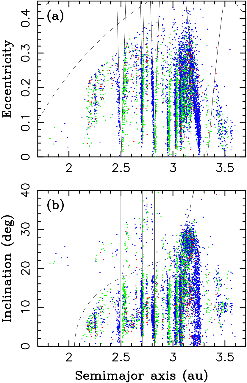
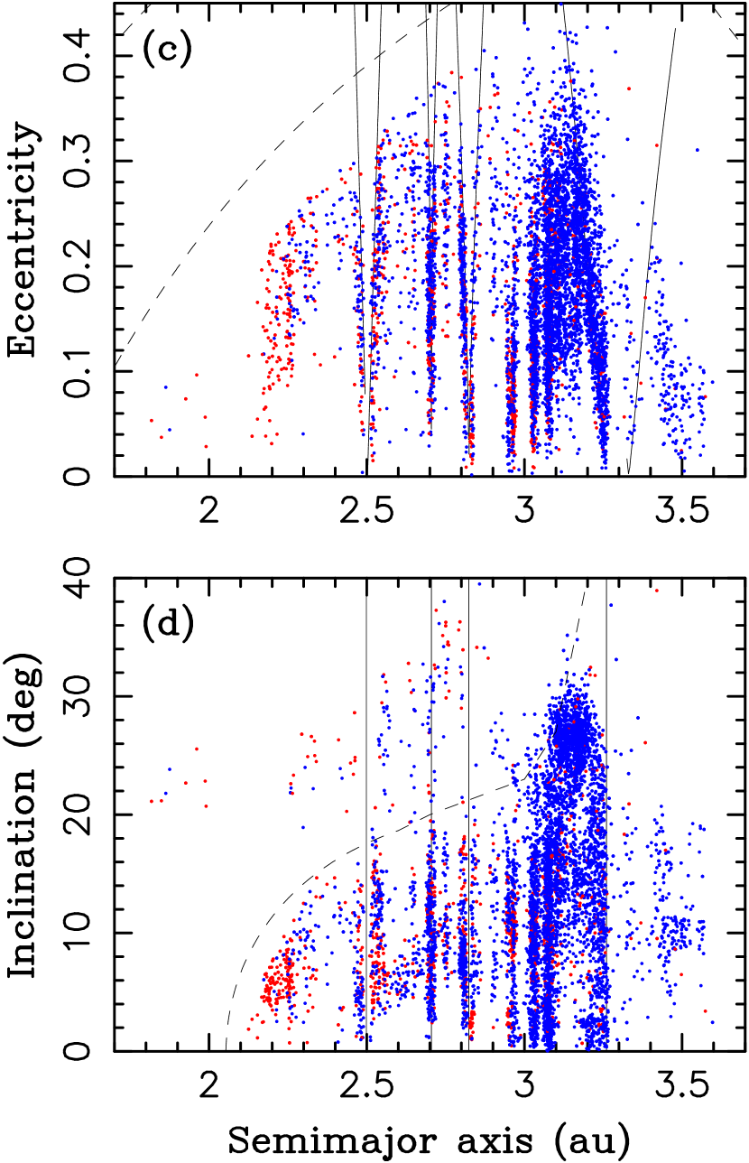
Figure 1: Panels (a) and (b): The initial orbits of $D>5$ km asteroids that escaped from the main belt in 0.4 Gyr. We only show the first 0.4 Gyr of our simulations, because the number of escaping MBAs in the model decays over time (Sect. 5.1), and we believe that the first 0.4 Gyr is the best choice to represent the long term average. The color indicates the Yarkovsky drift: ${\rm d}a/{\rm d}t=0$ (red), ${\rm d}a/{\rm d}t<0$ (green), and ${\rm d}a/{\rm d}t>0$ (blue). There is a clear preference for drift toward resonances. The clump of bodies at $a=3.1$–3.2 au and $i=25^{\circ}$–30^∘ is the Euphrosyne family. Panels (c) and (d): The same as (a) and (b) but now the color denotes the WISE albedo: blue for $p_{\rm V}\leq 0.1$ and red for $p_{\rm V}>0.1$. The thin solid lines show the location of orbital resonances with Jupiter. The dashed line in (a) and (c) is the Mars crossing limit. The dashed line in (b) and (d) is the secular resonance $\nu_{6}$.

The initial orbits of asteroids that escaped from the main belt in the course of our integration are highlighted in Fig. 1. Many more MBAs escape from the outer belt than from the inner belt, primarily because the outer belt represents a much larger source reservoir. For example, for $D>5$ km, there are 3373 bodies in the inner belt ($a<2.5$ au; 8% of the total number of $D>5$ km MBAs), 10178 bodies in the middle belt ($2.5<a<2.82$ au; between the 3:1 and 5:2 resonances with Jupiter; 24%), and 29170 bodies in the outer belt ($a>2.82$ au; 68%). The radial distribution of $D>10$ km bodies is similar (6%-21%-73%), but the overall number is $\simeq$5.2 times lower.

We now turn our attention to escape statistics. The number of MBAs escaping per 100 Myr slowly declines over time and the decline rate depends on the assumed Yarkovsky drift. Overall, there were 3211 clones escaping in $t<100$ Myr, 2295 in $100<t<200$ Myr, 2002 in $200<t<300$ Myr, 1678 in $300<t<400$ Myr, and 1565 in $400<t<500$ Myr (and the decline continues beyond 500 Myr). The decline is stronger when only clones with ${\rm d}a/{\rm d}t=0$ are considered, presumably because the escape resonances are not re-filled by new MBAs in this case. The decline is weaker for MBAs with the Yarkovsky drift: 1057 escape in $t<100$ Myr and 607 in $400<t<500$ Myr for ${\rm d}a/{\rm d}t<0$; 1140 for in $t<100$ Myr and 687 in $400<t<500$ Myr for ${\rm d}a/{\rm d}t>0$. Therefore, even in this case, the resonances are not refilled efficiently enough to keep the escape rate constant. This may either be real (i.e., the actual escape rate will decline in the future) or related to some dynamical effects that were not included in our model (e.g., caused by the Yarkovsky drift rate variability).

The escape rate of MBAs in the first 100 Myr of our simulations is considered the most realistic proxy for the present epoch. We find that one $D>5$ km asteroid escapes from the main belt every $\simeq$93 kyr, which means that $\simeq$2.5% of the whole population of $D>5$ km MBAs escape from the main belt in 100 Myr. Extrapolated to longer timescales this would represent one $e$-fold reduction of the original population every $\sim$4 Gyr, which is roughly consistent with the previous estimates (Minton and Malhotra, 2010; Nesvorný et al., 2017). Note, however, that this is somewhat coincidental because the previous works did not account for the Yarkovsky drift and adopted a random distribution of MBA orbits (including unstable orbits in resonances). For $D>10$ km, we determine that $\simeq 1.7$% MBAs escape in 100 Myr, which is identical to the estimate given in Nesvorný & Roig (2018).

We find that 123 $D>5$ km MBA clones were eliminated from the inner belt, 540 from the middle belt, and 2548 from the outer belt (all for $t<100$ Myr). These numbers correspond to 1.2%, 1.8%, and 2.9% of the populations in each zone. This means that the outer belt is more leaky than the inner belt probably because the outer MBAs have orbits opportunistically close to resonances at the current epoch. Combined with the much larger population of asteroids in the outer main belt, this implies that $\sim$21 times more MBAs escape from the outer belt than from the inner belt. Dark asteroids are predominant in the outer belt (e.g., the ${\rm d/b}$ ratio for $a>2.82$ au and $D>5$ km is $\simeq 3.7$; see footnote 3) and the escape statistics is therefore skewed toward dark asteroids as well. We find that 2588 dark ($p_{\rm V}\leq 0.1$) and 623 bright ($p_{\rm V}>0.1$) $D>5$ km MBAs escape in 100 Myr, indicating the overall $\simeq$4.2 preference for dark fugitives (Fig. 1c,d). Given the incomplete WISE sample, the preference may even be slightly higher if some dark outer belt MBAs are missing from the selected sample (Sect 4.1).

Most escaping asteroids start close to mean motion resonances with Jupiter, such as the 3:1, 8:3, 5:2, 7:3, 9:4, 11:5, and 2:1 (in the order of increasing semimajor axis). The bodies that start sunward from a resonance must have ${\rm d}a/{\rm d}t>0$ to reach the resonance (blue dots in Fig. 1a,b), whereas the bodies that started beyond a resonance must have ${\rm d}a/{\rm d}t<0$ (green dots in Fig. 1a,b). A relatively small fraction of the escaping MBAs are members of asteroid families (e.g., the Flora family at the inner edge of the asteroid belt, Nysa-Polana complex on the sunward side of the 3:1 resonance, Euphrosyne family at $3.1<a<3.2$ au and $25^{\circ}<i<30^{\circ}$; Masiero et al. 2015b). Overall, only $\sim 20$% of $D>5$ km NEAs are found to be previous members of known asteroid families (Sect. 5.3; Nesvorný et al., 2015).

5.2 Population of $D>5$ km NEAs

There are no NEAs in our simulations at $t=0$. By monitoring the number of model NEAs with time we find that it takes some time for the NEA population to build up. Interestingly, dark NEAs reach a steady state faster (in $\sim 10$ Myr) in our model than bright NEAs. This makes sense because there is a larger flux of dark NEAs from the middle and outer belts, but these NEAs have shorter dynamical lifetimes (Table 2, Sect. 5.3), which means that the steady state can be established faster than for bright NEAs (for which the situation is the opposite). We find that it takes $\sim 50$ Myr for bright NEAs to reach a steady state. After this time, both the dark and bright NEA populations start to slowly decline over hundreds of Myr, reflecting the diminishing influx in our model (Sect. 5.1). Below we report the results from $50<t<400$ Myr.

We find that the number of $D>5$ km NEAs, $n_{5}$, substantially fluctuates over time. Figure 2(a) shows the probability distribution of $n_{5}$. Here we only consider orbits with $q<1.3$ au and $Q<4.5$ au to avoid NEOs with a possible cometary origin (we do not model dormant comets here). Two models are plotted. The distribution that peaks for $n_{5}\simeq 6$ was obtained from all clones included in the integrations. This would correspond to a situation where it is equally probable to have maximum negative, zero, and maximum positive Yarkovsky drifts (hereafter the random drift model). The broader distribution that peaks for $n_{5}\simeq 11$ was obtained by optimizing the Yarkovsky drift. For that, we selected one clone for each MBA that escaped to a NEA orbit, assuming that such a clone exists for that MBA. If more than one clone escaped for the same MBA, we selected one escaping clone at random. The mean values are $\langle n_{5}\rangle=6.3$ and 12.6 in the models with the random and optimized drifts. Relative to the Poisson distribution $P(n)=e^{-\lambda}\lambda^{n}/n!$, where $n\geq 0$ and the occurrence rate $\lambda=11.5$ (the dashed line in Fig. 2(a)), the optimized distribution shows a slight excess of cases with $n_{5}<7$.

To compare our results with observations, we extracted all $D>5$ km NEAs from the WISE catalog (Mainzer et al., 2019). The basic information about these NEAs is listed in Table 1. We find that there are 17 NEAs with $q<1.3$ au, $Q<4.5$ au, and $D>5$ km. Three of these bodies have $D\simeq 5$ km (Table 1) but a rather large diameter uncertainty, and in reality can be smaller than 5 km. It is also possible that we missed some $D>5$ km NEAs either because they were not observed by WISE or because their diameter was sub-estimated from thermal modeling. For reference, Nugent et al. (2016) reported the diameter errors from WISE have $\sim 20$% (1$\sigma$) uncertainties.

The NEA model with random Yarkovsky drifts is clearly incompatible with observations (Fig. 2(a)). In that model, the probability to have $n_{5}\geq 17$ is $<10^{-5}$. The model with optimized drifts fares better: $n_{5}\geq 17$ is expected with the $\simeq$11% probability. Still, the current population of NEAs is larger than the long-term average, which may give support to the possibility that the present impact flux on the terrestrial worlds has increased $\sim 300$–400 Myr ago (e.g., Culler et al., 2000; Mazrouei et al., 2019; also see Kirchoff et al., 2021). The optimized model implies that MBAs are drifting toward resonances that lead to their ultimate escape from the main belt (and not away from them). This makes sense because if MBAs would be drifting away from resonances, they would need to start in the resonances, and would not exist in the first place (would be removed in the past). There are several potential caveats to this. For example, MBAs may jump over weaker resonances and may appear as drifting away from them at the present time.

The observed ratio of dark/bright NEAs with $D>5$ km is ${\rm d}/{\rm b}=8/9\simeq 0.9$ (Table 1). Figure 2(b) shows the ${\rm d}/{\rm b}$ distribution obtained in the model with optimized drifts (the distribution with random drifts is similar). As the number of large NEAs changes with time, the ratio of dark/bright NEAs changes as well. This is a consequence of the stochastic delivery process. Thus, depending on the considered time, it can be as low as $<0.5$ ($\sim 10$% probability) or as high as $>2$ ($\sim 5$% probability). The most likely values, however, are intermediate: the ratio distribution peaks near ${\rm d}/{\rm b}=0.8$ and the mean value is $\langle{\rm d}/{\rm b}\rangle=1.3$. There is thus a relatively good agreement with observations. With that said, however, it needs to be mentioned that the observations obtained at the current epoch and are not particularly constraining for the long-term average. For comparison, Morbidelli et al. (2020) estimated ${\rm d}/{\rm b}=1.3$ for small NEOs from calibrating the many-source model of G18 on the NEOWISE observations (Mainzer et al. 2019).

5.3 NEA Sources

We now consider the source regions of $D>5$ km NEAs. For that, we select all NEAs produced in our simulation for $50<t<400$ Myr and track these bodies back to their starting orbits. We find that the inner, middle and outer belts contribute by 52%, 35% and 13%, respectively. The percentages quoted here were obtained in the model with optimized drifts but the values for random drifts are similar (Table 3). We therefore estimate that MBAs with $a<2.5$ au and $a>2.5$ au supply roughly the same number of $D>5$ km NEAs. This implies a much larger contribution of the middle/outer main belt than found previously for small NEAs from the many-source models (B02, G18; see Sect. 6.1 for a discussion).

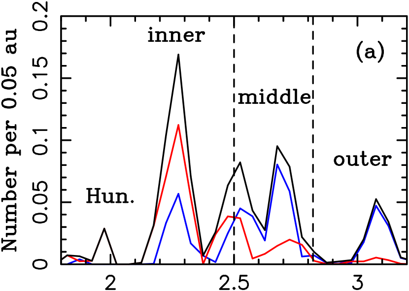
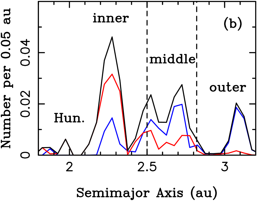
Figure 3: The contribution of MBAs to NEAs is shown here as a function of MBA’s starting semimajor axis (black solid lines). The blue/red solid lines show the main belt contribution to dark/bright $D>5$ km NEAs, respectively. The inner belt is the main source of bright NEAs and the middle belt is the main source of dark NEAs. The optimized drift model is shown in panel (a), random drift model in panel (b). Label “Hun.” stands for Hungarias.

For example, B02 determined from the many-source model that the combined contribution of $\nu_{6}$, IMCs and 3:1 is 84%, leaving only 16% for the outer belt and JFCs. We find that the contribution of MBAs with $a<2.55$ au, which includes $\nu_{6}$, IMCs and 3:1, is significantly lower, 61%, leaving a much larger contribution to the middle/outer belt (39%; Fig. 3). It is more difficult to compare our results to G18, because the seven sources used in that work included extended ‘complexes’ of escape routes near major resonances. To estimate the inner belt contribution from G18, we put together the contributions of Hungarias, Phoaceas, the $\nu_{6}$ complex, and the 3:1 complex. This gives 83%, which is similar to the estimate of B02, and leaves only 17% for the middle/outer belt and comets. Again, this is much lower than our 39%.

The differences discussed above may have several different interpretations: (i) The contribution of different sources is size-dependent; the many-source models were calibrated on $D\lesssim 1$ km NEOs, whereas here we have $D>5$ km. (ii) The many-source models, given the methodology caveats discussed in Sect. 2, may fail to properly weight in the contribution of MBAs with $a>2.5$ au. (iii) The contribution of different sources is time variable and the present NEO distribution – as characterized from many-source models – is not representative for the long term average. See Section 6.1 for a discussion. For Hungarias and Phoaceas, we find the 4.5% and 9.1% contributions, respectively, whereas G18 reported 5.6% and 2.7%. The reason behind the disagreement for Phoaceas is unclear.

In our single-source model, the contribution of MBAs with $a<2.5$ au and $a>2.5$ au to large NEAs is similar (52% and 48%, respectively; Table 3). This has interesting consequences for how the main belt supplies dark/bright $D>5$ km NEAs. The middle belt is the main contributor of dark NEAs (50%; Table 4, Fig. 3) and the inner belt is the main contributor of bright NEAs (76%). In B02 and G18, instead, where over 80% of NEOs originate in the inner belt, most dark NEAs also come from the inner belt (G18, Morbidelli et al. 2020). These differences may be related to some of the issues mentioned above. For example, they could reflect the size-dependent nature of the delivery process.

The contribution of asteroid families to $D>5$ km NEAs is minor. To determine this contribution, we link the $D>5$ km MBAs to the family catalog from Nesvorný et al. (2015). We find that only 20% of $D>5$ km NEAs in a steady state are expected to come from known families. The remaining 80% come from background MBAs. This estimate is consistent with Vokrouhlický et al. (2017), who found that the Flora family, which is optimally placed near the $\nu_{6}$ resonance to produce NEAs, contributes by only 3.5–5% to the $D>1$ km NEA population at the present time. The individual contribution of any other asteroid family to the present-day NEAs is low ($<1$% for $D>5$ km). The family contributions to smaller NEAs could be more significant because the collisional families generally have a steep size distribution for $D\lesssim 5$ km (Masiero et al., 2013, 2015b).

Dynamical lifetimes of NEAs are listed in Table 2. We find that the mean dynamical lifetime of $D>5$ km NEAs is $\langle t_{5}\rangle=1.2$ Myr, which is shorter than the $\sim 4$ Myr estimate from B02. This probably reflects a greater contribution of the middle/outer belt in our model. We identify a clear trend with the dynamical lifetime decreasing with the radial distance of a source. For example, MBAs evolving from the outer belt only spend, on average, $\simeq 0.5$ Myr on NEA orbits. Compared to Gladman et al. (1997), we find a good agreement for the 3:1 and 5:2 resonances ($\langle t_{5}\rangle=2.9$ and 0.7 Myr, respectively). For 8:3, which is an important source region of dark NEAs in the middle belt (Fig. 3), we estimate $\langle t_{5}\rangle=2.3$ Myr.

5.4 Orbital Distribution of Large NEAs

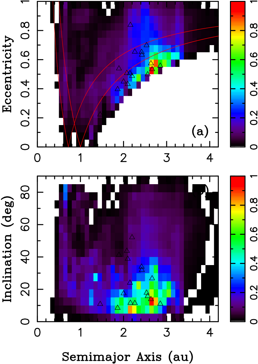
Figure 4: The orbital distribution of $D>5$ km NEAs obtained in our model with optimized drift rates. The binned residence times from our simulations are normalized to one and plotted here in the $(a,e)$ and $(a,i)$ projections. The color scale, which corresponds to the binned probability, appears on the right (warm colors indicate higher probability). The triangles show 17 known NEAs with $D>5$ km (Table 1).

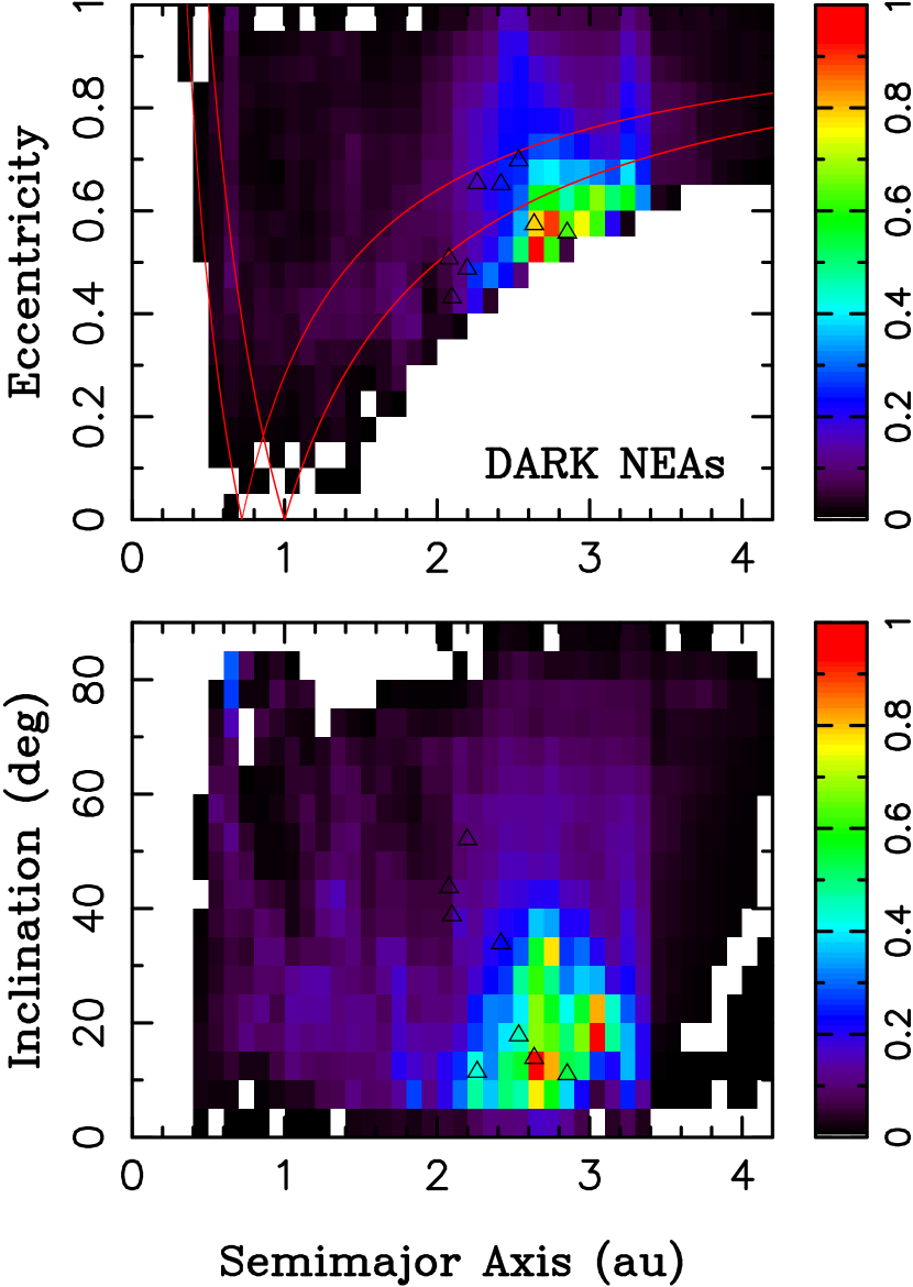
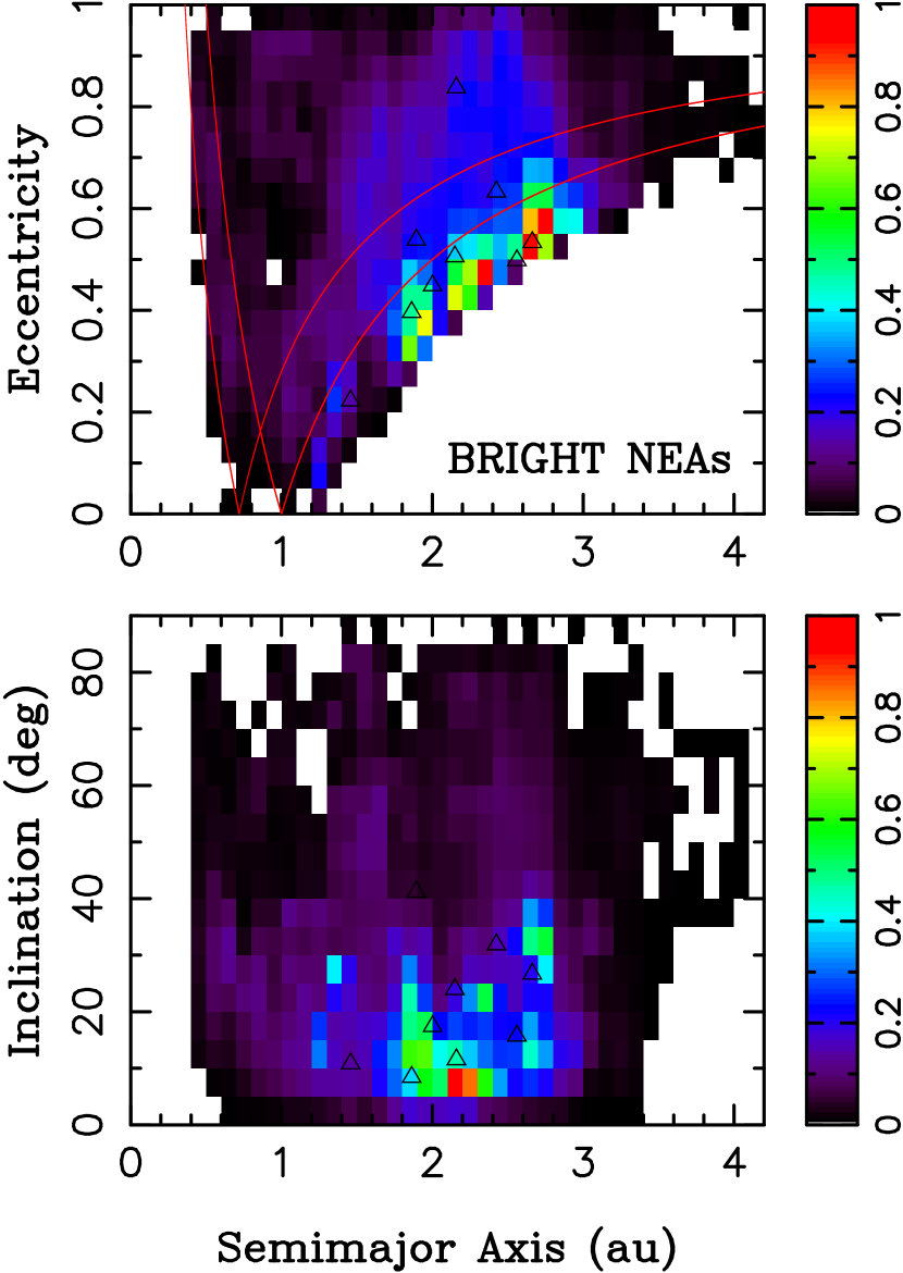
Figure 5: The orbital distribution of $D>5$ km NEAs obtained in our model: $p_{\rm V}\leq 0.1$ on the left and $p_{\rm V}>0.1$ on the right. The two distributions are slightly different: the highest probability for dark NEAs occurs for orbits $2.6<a<3.2$ au, whereas bright NEAs are expected to populate a wide radial range, $1.8<a<2.8$ au. The triangles show 8 known $D>5$ km NEAs with $p_{\rm V}\leq 0.1$ (left panels) and 9 known $D>5$ km NEAs with $p_{\rm V}>0.1$ (right panels).

Our single-source model can be used to determine the steady-state orbital distribution of large NEAs. Here, there is no need for observational calibration of different sources. The orbital distribution of NEAs is uniquely determined by the main belt structure and our (simple) physical model for the radiation forces. It represents a testable model prediction. Figure 4 shows the orbital distribution of $D>5$ km NEAs obtained in the model. The distribution peaks at $2<a<3$ au, $1<q<1.3$ au and $5^{\circ}<i<30^{\circ}$. Compared to B02 and G18, where similar plots were published for smaller NEAs, there are more orbits with $a>2.5$ au (and fewer orbits with $a<2.5$ au). Dark $D>5$ km NEAs are primarily responsible for this shift (Fig. 5, left panels). The middle/outer belt ($a>2.5$ au) supplies the majority of dark NEAs in our model (71% total contribution; Table 4), and this leads to a distribution that is skewed toward $a>2.5$ au. Bright $D>5$ km NEAs are distributed more equally between 2 and 3 au (Fig. 5, right panels).

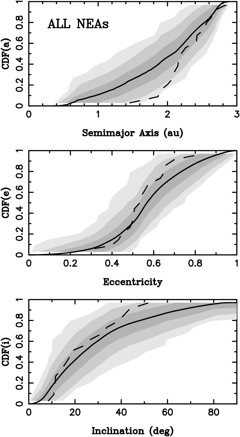
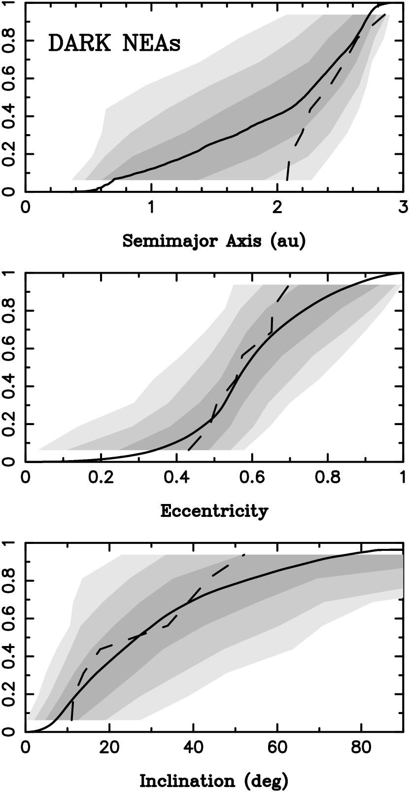
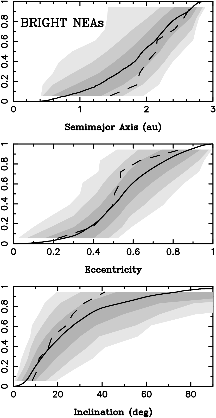
Figure 6: The cumulative distribution functions (CDFs): all NEAs (left panels), dark NEAs with $p_{\rm V}\leq 0.1$ (middle panels), and bright NEAs with $p_{\rm V}>0.1$ (right panels). The solid and dashed lines show the optimized model and observed distributions for $D>5$ km NEAs, respectively. The shaded ares are an expression of the statistical uncertainty: 1$\sigma$ (68.2%, dark gray), 2$\sigma$ (95.4%, grey), and 3$\sigma$ (99.7%, light grey). To define these areas we sub-sampled the model results to the number of real NEAs in each category (17 for all, 8 for dark, 9 for bright), generated 1000 sub-sampled distributions, and defined each envelope to contain the appropriate percentage of trials.

We compare the model distributions with observations in more detail in Fig. 6. Unfortunately, the number of $D>5$ km NEAs is statistically small and the comparison is not particularly constraining. A potential problem is identified in the semimajor axis distribution (or, equivalently, the perihelion distance distribution). This is particularly clear for dark NEAs, where all 8 known NEAs with $D>5$ km and $p_{\rm V}\leq 0.1$ have $a>2$ au, whereas our model suggests that $\sim$40% of dark/large NEAs should have $a<2$ au. Statistically, this represents odds of $0.6^{8}\simeq 1.7$% (i.e., between 2$\sigma$ and 3$\sigma$). When the dark and bright NEAs are combined, the statistics improves (left panels in Fig. 6), but the semimajor axis difference remains below 3$\sigma$. The small number statistics has a heavy influence on this comparison. In addition, our simulations ignore Mercury (Sect. 4.3), and we are therefore not fully confident that the orbital distribution of model NEAs with low perihelion distances is correct.

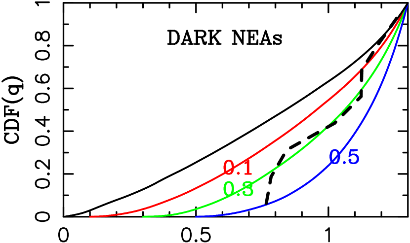
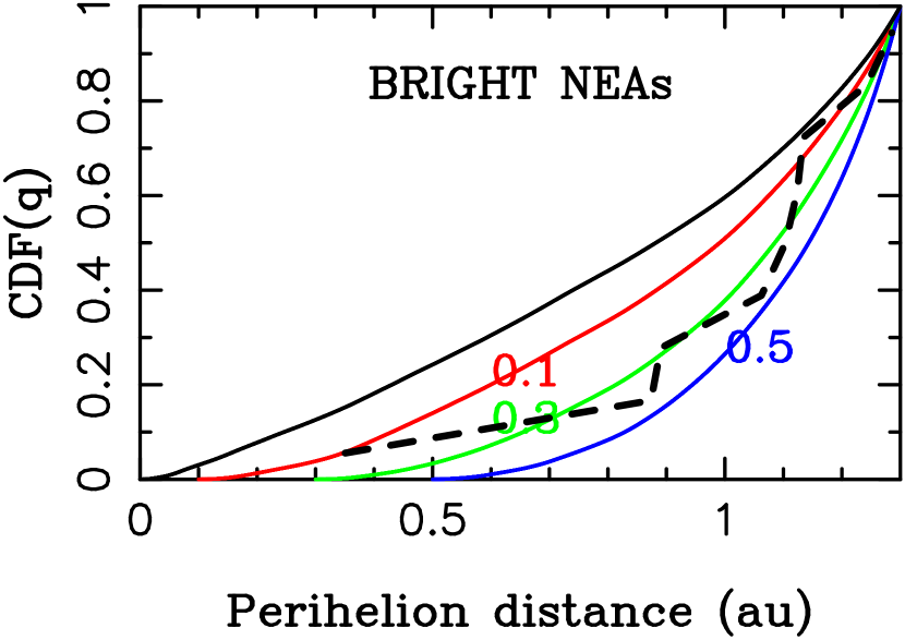
Figure 7: The perihelion distribution of $D>5$ km NEAs: dark ($p_{\rm V}\leq 0.1$) in the top panel and bright ($p_{\rm V}>0.1$) in the bottom panel. The solid lines correspond to different models. The black line is the nominal model from Fig. 6; the large statistical uncertainty is not shown here. The color lines correspond to the models where NEAs evolving to $q<q^{*}$ were removed: $q^{*}=0.1$ au (red), $q^{*}=0.3$ au (green), and $q^{*}=0.5$ au (blue). The dashed line is the perihelion distribution of known $D>5$ km NEAs. Only one of 17 known $D>5$ km NEAs has $q<0.7$ au (2212 Hephaistos with $p_{\rm V}=0.16$ and $q=0.35$ au).

Despite these important caveats, we investigated models where NEAs reaching perihelion distance $q<q^{*}$, where $q^{*}$ is a free parameter, are removed. This is motivated by the possibility that thermal stresses close to the Sun could break up mechanically weak NEAs (Delbo et al. 2014, Granvik et al. 2016). A prime example of this is 3200 Phaethon with $q=0.14$ au, the parent body of the Geminid meteoroid stream, which episodically loses mass at an average rate of $\sim 700$ kg s^-1 (Jewitt et al. 2019). The best match to the observed distribution is obtained for $0.1\lesssim q^{*}\lesssim 0.3$ au (Fig. 7). This could suggest that large NEAs (gradually?) disintegrate when their orbital perihelion drops below 0.1-0.3 au. For comparison, Granvik et al. (2016) suggested that $D\lesssim$ 1 km NEAs super-catastrophically disrupt for $q\lesssim 0.1$ au.

5.5 Impact Flux from Large NEAs

In total, including all clones, 119 impacts of $D>5$ km asteroids were recorded on Venus (52 impacts), Earth (49) and Mars (18) in 1 Gyr (Fig. 8). Thus, in the random drift model, we infer $49/3\simeq 16$ $D>5$ km asteroid impacts on the Earth in 1 Gyr. The impact rate is about twice as high in the optimized drift model. We thus estimate $\sim$16–32 $D>5$ km asteroid impacts on the Earth in 1 Gyr, and the average time between impacts $\sim 30$–60 Myr. The impact flux on Venus is similar, and Mars receives roughly 37% of the terrestrial flux (i.e., the Earth-to-Mars impact flux ratio for $D>5$ km asteroids is $\sim 2.7$).

Previous studies of small NEOs estimated that the average impact probability for one object in the NEO population is $p_{\rm i}=1.5\times 10^{-3}$ Myr^-1 (Stuart 2001, Harris & D’Abramo 2014) or $p_{\rm i}=1.3\times 10^{-3}$ Myr^-1 (Morbidelli et al. 2020). When these probabilities are multiplied by the number of known $D>5$ km NEAs (17; Table 1), we compute $\simeq$22–26 impacts on the Earth in 1 Gyr, which would be consistent with our estimate from the recorded impacts. It is not clear, however, whether this comparison is strictly correct because of different definitions of the NEA/NEO target regions in different works (e.g., $a<4.2$ au in G18 and Morbidelli et al. (2020), but $Q<4.5$ au here). If NEOs with $a<4.2$ au and $Q>4.5$ au were included here, the number of impacts estimated from $p_{\rm i}$ would be higher.

For comparison, Johnson et al. (2016), adopting $p_{\rm i}=1.5\times 10^{-3}$ Myr^-1 and using absolute magnitude as a proxy for size, estimated $\sim$50 impacts of $D>5$ km asteroids on the Earth in 1 Gyr, which is 1.6-3.1 times higher than our value. Nesvorný et al. (2017) and Nesvorný & Roig (2018) estimated that only $\sim 1$ impact of a $D>10$ km asteroid should occur on the Earth over 1 Gyr. Here we find $\sim 2$ such impacts in the random drift model. Ignoring the Yarkovsky effect and rescaling from $D>10$ km to $D>5$ km from the MBA-inferred ratio of $\sim$5.2 (Sect. 5.1), we would infer only $\sim 10$ impacts of $D>5$ km asteroids on the Earth per 1 Gyr. Our best estimate is $\sim 1.6$–3.2 times higher than that. This means that the Yarkovsky effects kicks in for $D<10$ km and generates more $D>5$ km NEAs than what would be expected from a simple scaling based on the size distribution of MBAs.

We see some variability when the impact statistics obtained in our model is sliced in time (e.g., the number of impacts in a 100-Myr interval fluctuates by a factor of $\sim 2$), but no long-term trends (there are 56 impacts in $0<t<0.5$ Gyr and 63 impacts in $0.5<t<1$ Gyr). Here we therefore report the results for the full 1-Gyr interval, where we have the best statistics. There were 72 impacts (60%) from bodies starting with $a<2.5$ au and 47 impacts (40%) from $a>2.5$ au. The inner belt thus supplies somewhat more impactors on the terrestrial worlds, $\sim 1.5$ times more, than the middle/outer belt. For comparison, G18 reported that $\sim$80% of terrestrial impactors with absolute magnitudes $17<H<22$ ($0.17<D<1.7$ km for $p_{\rm V}=0.1$) come from the $\nu_{6}$ resonance at the inner edge of the main belt. Relative to this, the middle/outer belt has a much larger importance as the source of large terrestrial impactors.

We find that 47% of large terrestrial impactors are dark ($p_{\rm V}\leq 0.1$) and 53% are bright ($p_{\rm V}>0.1$), suggesting a roughly equal split (Table 5). About 59% of dark impactors come from the middle/outer belt ($a>2.5$ au). In contrast, most small and dark impactors on the Earth start in the inner belt (B02; G18), suggesting a size-dependent sampling of the main belt.

About 78% of bright $D>5$ km terrestrial impactors originate in the inner belt ($a<2.5$ au). Of these, 11 impactors (18%) were previous members of the Flora family. In total, the asteroid families contribute by only 23% to impacts of $D>5$ km asteroids on the terrestrial worlds (this estimate does not account for impactors from the family halos; Nesvorný et al., 2015). Other notable families with more than one recorded impact are: Euphrosyne (3 impacts representing 5% of dark impactors; cf. Masiero et al. 2015a), Koronis (3 impacts) and Dora (2 impacts). This implies that a great majority of large terrestrial impactors are not previous members of the asteroid families – they are background MBAs.

The statistics of impacts discussed above would be affected if NEAs break up when they evolve too close to the Sun (Sect. 5.4). We investigated this effect and found that the number of impacts on the Earth drops to 67% for $q^{*}=0.1$ au and 51% for $q^{*}=0.3$ au (both percentages quoted with respect to the nominal 100% impact flux without the NEA removal). The effect is stronger for Venus (48% for $q^{*}=0.1$ and 31% for $q^{*}=0.3$ au) and weaker for Mars (only a 5% reduction of the number of impacts for both $q^{*}=0.1$ and 0.3 au). We did not find any obvious dependence of the removal effect on the NEA source (inner vs. outer belt) or type (dark vs. bright).

The pre-impact orbits are shown in Fig. 9. These are the orbits of $D>5$ km impactors on the terrestrial planets just before their final dive toward an impact (the orbits are computed at 3 Hill radii from a planet). The Venus and Earth impactors have a wide orbital distribution with large eccentricities and large inclinations. Most impacts on the Earth happen from orbits with $0.8<q<1$ au; that is where the impact probabilities are the highest (Bottke et al. 2020). For Mars, 11 out of 18 pre-impact orbits (61%) have $a>2$ au, $q>1.4$ au and $i<10^{\circ}$. Most $D>5$ km Mars impactors reach the Mars-crossing orbits via weak resonances (Migliorini et al., 1998), and apparently impact before their perihelion distance evolves too much (Fig. 9).

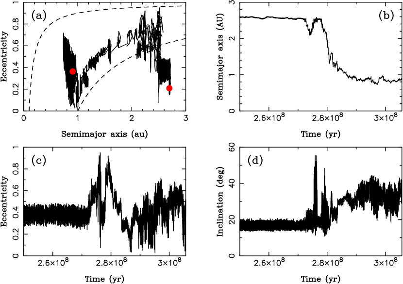
Figure 11: The orbital history of asteroid 209192 ($D\simeq 5.7$ km, $p_{\rm V}\simeq 0.04$, assumed ${\rm d}a/{\rm d}t>0$) that started just below the 8:3 resonance and ended impacting on the Earth. The red dots in panel (a) show the initial and final orbits. We also plot $q=0.1$ au and $q=1$ au for a reference (dashed lines in (a)). This specific MBA clone started sunward of the 8:3 resonance with Jupiter and drifted into the resonance with ${\rm d}a/{\rm d}t>0$. It subsequently reached a Mars-crossing orbit and evolved to the 3:1 resonance with Jupiter by distant encounters with Mars. The 3:1 resonance transferred the asteroid to NEA space, where it impacted on the Earth at $t=306$ Myr.

The mean impact speeds are listed in Table 6 and the distribution of impact speeds is shown in Figure 10. We find that the mean impact speed of $D>5$ km NEAs on the Earth is nearly twice as large as the one on Mars (20.3 vs. 10.6 km s^-1). For Mars, about 60% of impacts happen with the relatively low impact speeds $v_{\rm imp}<8$ km s^-1. Venus shows much larger impact speeds with $\sim 25$% of impactors having $v_{\rm imp}>40$ km s^-1 (Fig. 10). Moreover, 3 out of 52 Venus impactors (6%) evolved to a retrograde orbit before the impact, and hit Venus at speeds exceeding 60 km s^-1. No such very-high-speed impact was recorded on the Earth but that is probably just an issue of small number statistics. The impact speeds of bright and dark asteroids are similar (e.g., terrestrial impacts with mean $v_{\rm imp}=20.5$ km s^-1 for bright and mean $v_{\rm imp}=20.0$ km s^-1 for dark). Dark asteroids often evolve to small orbital radii before they impact (see Fig. 11 for an example).

6 Discussion

6.1 Comparison with Many-Source Models

Compared to B02 and G18, here we find a larger contribution of the middle/outer belt to NEAs/impactors. For example, G18 estimated that the contribution of outer MBAs to NEAs is practically negligible ($\simeq 3.5$% for the 2:1 resonance complex). They found that $\simeq 80$% of impactors on the terrestrial worlds are produced from the $\nu_{6}$ resonance, and over 10% from the 3:1 resonance, Hungarias and Phoaceas, leaving $<10$% for the middle/outer belt. Based on this, G18 suggested that the majority of primitive NEOs/impactors come from the $\nu_{6}$ resonance. Here we find, instead, that the middle/outer belt supplies nearly 50% of NEAs, $\simeq$70% of dark NEAs, and $\simeq 35$–40% of large impactors.

These differences may be a consequence of the size-dependent delivery process. On one hand, small MBAs can drift over a considerable radial distance by the Yarkovsky effect and reach NEA space from the powerful $\nu_{6}$ resonance at the inner edge of the asteroid belt (e.g., Granvik et al., 2017). The $\nu_{6}$ resonance is known to produce highly evolved NEA orbits and impact probabilities on Earth in excess of 1% (Gladman et al. 1997). On the other hand, large MBAs often reach NEA orbits via slow orbital evolution in weak resonances (Migliorini et al., 1998; Morbidelli and Nesvorný, 1999; Farinella and Vokrouhlický, 1999). Figure 11 shows an example for the 8:3 resonance. Whereas each of these resonances contributes only a little, their total contribution to the population of large NEAs is significant. This can explain the more even contribution of different radial zones of the main belt to large NEAs.

Whether the transition from the $\nu_{6}$-controlled statistics for small asteroids to a more even contribution for large asteroids really happens for $1\lesssim D\lesssim 5$ km has yet to be established. Our results strictly apply for $D>5$ km. The single-source model could be extended to $D<5$ km, but this would require to develop a more realistic model for the YORP/Yarkovsky effects and collisions, and is left for future work. The many-source model of G18 was developed for $H>17$ ($D<1.7$ km for $p_{\rm V}=0.1$), where the model results can be calibrated on a large number of NEO detections by the Catalina Sky Survey (Christensen et al., 2012; Jedicke et al., 2016). The many-source model could be extended to $H<17$, but this is difficult to do with confidence because there are far fewer large NEO detections, and the calibration method would be affected by statistical uncertainties.

Alternatively, the tension between the single- and many-source model results could be related to the time variability of the NEO population/impactor flux. The many-source models are calibrated on the currently observed population of NEOs, whereas our single-source model deals with the long-term average. There are all sorts of interesting issues that may arise from time variability. For example, it has been suggested that the cratering rate in the inner Solar System increased by a factor of $\sim$2-4 about 300-400 Myr ago (e.g., Culler et al., 2000; Mazrouei et al., 2019). If that is the case, we may be living in an epoch when the NEO population is $\sim$3 times larger than the long-term average (Fig. 2(a)). Catastrophic breakups of large parent MBAs near resonances can be responsible for changes of the NEA population/impactor flux. For example, the formation of the Flora family at the inner edge of the asteroid belt – near the $\nu_{6}$ resonance – was probably responsible for a factor of $\sim 2$ increase in the number of impacts 1-1.5 Gyr ago (Vokrouhlický et al., 2017).

Finally, some of the differences between the single- and many-source models may be a consequence of the adopted methodologies. The many-source models are agnostic to the radial distribution of MBAs (B02; Greenstreet et al., 2012; G18; Morbidelli et al., 2020). They do not take into account the availability of MBAs in (and near) different sources. This may potentially create a conflict between what is needed and what is available. For example, the many-source model can give a very strong weight to the $\nu_{6}$ resonance even if there are not enough asteroids near the $\nu_{6}$ resonance to justify it. One also needs to factor in that the outer belt has $\sim$10 times more MBAs than the inner belt (Sect. 5.1). The single-source model takes this into account but may have deficiencies elsewhere. For example, the simple physical model of radiation effects that we adopt here may fail to realistically emulate how MBAs reach resonances. Additional work is needed to improve our model and validate the results reported here.

6.2 Albedo and Taxonomy of Large/Small NEOs

Observations of NEOs/MBAs in near-infrared reveal a bimodal distribution of visible albedos (e.g., Mainzer et al., 2011a, 2012; Masiero et al., 2012, 2014; Wright et al., 2016). The two albedo groups, roughly $p_{\rm V}\leq 0.1$ and $p_{\rm V}>0.1$, which is the definition of dark and bright bodies that we adopt throughout this paper, are neatly correlated with the taxonomic classification of asteroids (Mainzer et al., 2011b; Pravec et al. 2012). The C-complex asteroids, representing primitive, carbonaceous-rich bodies thought to be implanted in the asteroid belt from the giant planet region (e.g., Walsh et al., 2011; Levison et al., 2009), are dark. The S-complex asteroids, representing an alphabet soup of different asteroid classes related to ordinary chondrites, HEDs, and other types of stony meteorites, are typically bright. The mean albedos of C- and S-complex asteroids are $p_{\rm v}=0.057$ and 0.197, respectively (Pravec et al., 2012).

The albedo-based classification of different asteroid types is only approximate – e.g., some S types can be dark if churned by impacts (Britt and Pieters, 1991) – but it is adopted here as a rough guide. In Table 1, we show that 7 $D>5$ km NEAs that have been taxonomically classified as S (Binzel et al., 2019) all have $p_{\rm V}>0.1$, and 4 $D>5$ km NEAs that have been classified as C (3 cases) or D (1 case) all have $p_{\rm V}\leq 0.1$ (dark D-type NEOs on cometary orbits with $Q>4.5$ au are not considered here). The C-type asteroids, which are the dominant type among dark NEAs/MBAs (D and P asteroids are more common among Hildas and Jupiter Trojans; Emery et al., 2015), are thought to be the parent bodies of carbonaceous chondrite (CC) metorites (e.g., Clark et al. 2011). Here we therefore adopt a schematic view that: “dark” equals to “primitive C type” equals to “carbonaceous chondrite”. The results reported here can therefore be used, with some caution, to understand the significance of CC material for NEAs and terrestrial impacts (Sect. 6.3).

We found that dark bodies represent $\sim 50$% of $D>5$ km NEAs (and $\simeq 45$% of $D>5$ km terrestrial impactors). Such a large share may be surprising because many previous works suggested that the primitive/dark NEOs should be less common. For example, Mainzer et al. (2012) reported that NEAs with $p_{\rm V}<0.1$ represent $\simeq 39$% of NEOs observed by WISE, and Binzel et al. (2019) reported that C-type NEAs represent only $\simeq 20$% of taxonomically classified bodies. The statistic inferred from infrared observations is insensitive to the visible albedo (Mainzer et al. 2015), but it still contains an orbital bias, because dark NEAs typically have larger orbits than bright NEAs and are therefore fainter and harder to detect in any wavelength (Fig. 4). Complex selection, albedo and orbital biases affect the taxonomic observations as well. This means that the share of dark C-type NEAs should be larger than reported in Mainzer et al. (2012) and Binzel et al. (2019).

Morbidelli et al. (2020) investigated this issue in the many-source model of G18 and found that dark bodies ($p_{\rm V}\leq 0.1$) represent $\simeq 57$% of the total population of small NEOs (in the unbiased, size-limited sample). This is fully consistent with the results obtained here (Table 1 and Fig. 2(b)). The fact that small (Morbidelli et al. 2020) and large (this work) NEOs have roughly the same share of primitive dark bodies is intriguing. In Sect. 6.1 we argued that the single- and many-source models are giving different results because the statistics obtained in these models may depend on asteroid size. If the statistics were strongly size dependent, however, we would expect that dark bodies should represent a smaller share of small NEAs (than found here for large NEAs). But this is not the case.

6.3 Implications for K/Pg-Scale Impacts

The Cretaceous-Paleogene (K/Pg) boundary $\simeq 66$ million years ago corresponds to one of the three largest mass extinction events in the past 500 million years (Alroy 2008). It famously ended the age of dinosaurs. The K/Pg mass extinction is thought to have been triggered by a large asteroid impact (Alvarez et al., 1980) just off the coast of the Yucatan peninsula, forming a 180-km-wide Chicxulub crater (Schulte et al., 2010). The impactor that produced the Chicxulub crater is estimated to be at least 10 km in size hitting the Earth surface at a steep angle 45–60^∘ to horizontal (Collins et al., 2020). Chromium found in sediment samples taken from different K/Pg boundary sites (Shukolyukov and Lugamir, 1998; Trinquier et al., 2006; Goderis et al., 2013), as well as a meteorite found in K/Pg boundary sediments from the North Pacific Ocean (Kyte et al., 1998), suggest the impactor was a CM-type carbonaceous chondrite (CC). This classification rules out the possibility that the K/Pg impactor came from an S-complex asteroid.

The CC composition of the K/Pg impactor is surprising because the dominant extraterrestrial material hitting Earth appears to be ordinary chondrites (OCs; e.g., Maier et al., 2006; Koeberl et al., 2007, Tagle et al., 2009). For example, from about a dozen terrestrial craters with diameters $D_{\rm cra}=10$–100 km and known (or suspected) impactor composition (Schmieder and Kring, 2020) only the Zhamanshin crater is believed to have been produced by a carbonaceous chondrite (Magna et al., 2017). In contrast, Chicxulub is one of only four recognized terrestrial craters with $D_{\rm cra}>100$ km, the other three being Popigai, Sudbury and Vredefort. The 36.6-Myr old, $D_{\rm cra}\simeq 100$ km Popigai crater in central Russia was produced by an OC impactor (Tagle and Claeys, 2005). The impactor types for the much larger and older Sudbury and Vredefort craters are uncertain, but if the Zaonega spherule layers are linked to the Vredefort impact (Mougel et al., 2017), they would indicate a CC composition of the impactor. In summary, $\sim 25$–75% of the largest craters on the Earth were produced by CC impactors.

The inferred composition of the K/Pg impactor is an important clue to its origin. It has been suggested, for example, that the K/Pg impactor may have been a fragment of a large, inner-main-belt asteroid that catastrophically disrupted 100-200 Myr ago, and left behind the Baptistina family (Bottke et al., 2007; Masiero et al., 2012). Subsequent infrared and spectroscopic observations revealed, however, that the Baptistina family probably does not have the right composition ($p_{\rm V}\simeq 0.18$ albedo from WISE and S-type spectrum; Reddy et al., 2011). The flux of cometary impactors is negligible compared to asteroids (e.g., dormant JFCs contribute by $<$1%; G18). Siraj and Loeb (2021) proposed that the impactor was a piece of a large long-period comet that tidally disrupted near its perihelion. This exotic idea has a number of problems, including the very low likelihood of terrestrial impacts from the long-period comets, the low efficiency of tidal disruption to make $D\gtrsim 10$ km fragments, and the general assumption that the geochemical signature of a cometary impactor would be consistent with the CM composition inferred for the K/Pg impactor.

Here we argue that the problem at hand may have a simple solution, because nearly a half of large terrestrial impactors are dark primitive asteroids with composition that is consistent with carbonaceous chondrites (via the relationship of low asteroid albedo to the C-type taxonomy and CC composition; e.g., Mainzer et al., 2011a; Pravec et al., 2012; Binzel et al., 2019). By modeling the orbital evolution of large MBAs, we show that large asteroids escape from the main belt via weak resonances (see Fig. 11 for an example). The large NEAs more evenly sample the radial extension of the main belt (Sect. 5.3), including the middle/outer belt where dark, C-type asteroids are quite common (Sect. 5.1). That is why the large terrestrial impactors are often (in $\simeq 45$% of cases; Table 5) dark primitive bodies with a (plausible) CC composition. Small, $D\lesssim 1$ km terrestrial impactors have predominantly OC composition because their delivery from the main belt is controled by the powerful $\nu_{6}$ resonance at the inner edge of the asteroid belt (where the OC material is common; Sect 5.1).

Our model with random Yarkovsky drifts indicates $\sim 2$ $D>10$ km asteroid impacts on the Earth in 1 Gyr. This is about a factor of 2 higher than the impact flux inferred in Nesvorný and Roig (2018), possibly because the Öpik code used in that work had underestimated the number of impacts. The NEA population and impact rates tend to be up to a factor of $\sim 2$ higher with optimized Yarkovsky drifts (Sect. 5.2 and 5.5). We therefore find that $\sim$2-4 impacts of $D>10$ km asteroids should happen on the Earth in 1 Gyr and that the average spacing between impacts should be $\sim 0.25$–0.5 Gyr This is a useful input for understanding the frequency of impact-related mass extinctions on the Earth. About half of these large impactors are carbonaceous chondrites (see above). Having at least one mass extinction from a $D>10$ km impact happening in the last 100 Myr, for example, is a roughly a 20-40% probability event, or a 10-20% probability event if the CC composition of the Chicxulub impactor is factored in.

7 Conclusions

We conducted dynamical simulations of known $D>5$-km main-belt asteroids as they evolve onto NEA orbits by radiation forces and resonances. The results were used to develop a single-source model for large NEAs and terrestrial impactors. The main advantage of the single-source model is that it takes into account the availability of MBAs near source resonances. Our main findings are:

1. The NEA model with random Yarkovsky drifts is incompatible with the number of observed $D>5$ km NEAs ($n_{5}=17$; Table 1). This could mean that the current population of large NEAs is a factor of $\sim$2-3 larger than the long-term average (Mazrouei et al. 2019). In the model with Yarkovsky optimized drifts there is a $\simeq$11% probability to have $\geq 17$ $D>5$ km NEAs at any single epoch.

2. The long-term average of the ratio of dark ($p_{\rm V}\leq 0.1$) and bright ($p_{\rm V}>0.1$) $D>5$ km NEAs peaks near 0.8 and the mean value is 1.3. There is a good agreement with current observations which show 8 dark and 9 bright $D>5$ km NEAs (i.e., $\sim 0.9$ ratio).

3. Nearly 50% of diameter $D>5$ km NEAs start in the middle/outer belt ($a>2.5$ au) and reach NEA orbits via weak orbital resonances (e.g., the 8:3 resonance with Jupiter at 2.7 au). The middle belt is the main contributor of dark NEAs (50%) and the inner belt is the main contributor of bright NEAs (76%).

4. The contribution of asteroid families to $D>5$ km NEAs is relatively minor. We find that only 20% of $D>5$ km NEAs in a steady state are expected to originate in known families. The remaining 80% are background MBAs. The family contributions to dark and bright $D>5$ km NEAs are the same.

5. Our model fails to match – but only at 2–3$\sigma$ – the semimajor axis and perihelion distance distributions of observed $D>5$ km NEAs. For $p_{\rm V}\leq 0.1$, the model suggests that $\sim$40% of large NEAs should have $a<2$ au or $q<0.7$ au, but all 8 known $D>5$ km NEAs with $p_{\rm V}\leq 0.1$ have $a>2$ au and $q>0.7$ au. We investigated models where NEAs with $q<q^{*}$ are removed (e.g., disrupted by thermal stresses) and found $0.1\lesssim q^{*}\lesssim 0.3$ au would provide a better match to observations.

6. The time-averaged impact flux of $D>5$ km asteroids on the Earth is $25\pm 7$ Gyr^-1, where the uncertainty expresses the dependence of the model results on the distribution of MBA spin vectors (that influence the Yarkovsky drift and influx of MBAs on NEA orbits). Venus receives about the same number of impacts as the Earth, and Mars receives $\simeq 2.7$ fewer impacts than the Earth.

7. MBAs starting with $a>2.5$ au produce 35–40% of $D>5$ km asteroid impacts on the terrestrial planets. For comparison, G18 reported that $\simeq 80$% of the terrestrial impactors with absolute magnitudes $17<H<22$ ($0.17<D<1.7$ km for $p_{\rm V}=0.1$) come from the $\nu_{6}$ resonance at the inner edge of the main belt. This suggest that the contribution of different parts of the main belt to terrestrial impacts is size dependent.

8. We find that 47% of large terrestrial impactors are dark ($p_{\rm V}\leq 0.1$) and 53% are bright ($p_{\rm V}>0.1$), suggesting a roughly equal split. About 60% of dark impactors come from the middle/outer belt ($a>2.5$ au). In contrast, according to G18, most small/dark impactors on the Earth come from the inner belt.

9. Nearly 80% of bright $D>5$ km impactors start in the inner belt ($a<2.5$ au). Of these, 18% were previous members of the Flora family. In total, the asteroid families contribute by 23% to impacts of $D>5$ km asteroids on the terrestrial worlds.

10. The number of impacts on the Earth impacts drops to 67% for $q^{*}=0.1$ au and 51% for $q^{*}=0.3$ au (both percentages quoted with respect to the original impact flux without the NEA removal). The removal effect on impacts is stronger for Venus (48% for $q^{*}=0.1$ au and 31% for $q^{*}=0.3$ au), and negligible for Mars.

11. The mean (median) impact velocities of large NEAs are 30.5 (27.9), 20.3 (19.3) and 10.6 (7.6) km s^-1 for Venus, Earth and Mars, respectively.

The findings reported here have important implications for our understanding of the occurrence rate and nature of the K/Pg-scale impacts on the terrestrial worlds. Impacts of $D>10$ km asteroids on the Earth do not happen often (average spacing $\sim 250$–500 Myr), implying that having one K/Pg-scale event in the past 100 Myr was mildly special ($\sim 10$–40% probability; see discussion in Sect. 6.3). About a half of large terrestrial impactors are expected to be dark carbonaceous asteroids.

number	name/desig.	$a$	$e$	$i$	$D$	$p_{\rm V}$	tax.
		(au)		(∘)	(km)
433	Eros	1.458	0.223	10.8	16.8	0.25	S
1036	Ganymed	2.663	0.534	26.7	36.5	0.23	S
1580	Betulia	2.197	0.488	52.1	6.5	0.07	C
1627	Ivar	1.863	0.397	8.5	8.1	0.13	S
1866	Sisyphus	1.893	0.539	41.2	6.6	0.26	S
1917	Cuyo	2.149	0.506	24.0	5.0	0.20	-
2212	Hephaistos	2.160	0.838	11.6	5.5	0.16	S
4954	Eric	2.002	0.449	17.4	8.9	0.19	S
5731	Zeus	2.263	0.654	11.4	6.9	0.02	-
7092	Cadmus	2.535	0.698	17.8	6.3	0.05	-
20826	2000 UV13	2.425	0.633	31.9	5.9	0.12	-
25916	2001 CP44	2.561	0.498	15.7	5.8	0.22	S
26760	2001 KP41	2.853	0.557	11.0	5.4	0.04	C
52762	1998 OR2	2.418	0.652	33.9	6.7	0.05	D
88263	2001 KQ1	2.097	0.432	38.8	5.1	0.04	-
89830	2002 CE	2.077	0.507	43.7	5.1	0.08	-
162566	2000 RJ34	2.636	0.574	13.9	6.0	0.03	C

Table 1: A list of $D>5$ km NEAs from WISE (Mainzer et al., 2019). The taxonomic type in the last column was taken from Binzel et al. (2019). In the cases where more than one albedo/diameter measurements were available from WISE, we report the arithmetic mean of these measurements. Given the reported uncertainty of WISE-inferred size estimates ($\sim 20$% 1$\sigma$ uncertainty; Nugent et al. 2016), some of these NEAs may actually have $D<5$ km. This is especially relevant for 1917 (bright), 88263 (dark) and 89830 (dark). We include these cases here for completeness. 3200 Phaethon, the target of future JAXA’s DESTINY mission, has $D\simeq 4.2$ km from AKARI (Usui et al., 2011), $D\simeq 4.6$ km from WISE (Masiero et al., 2019), $D\simeq 5.1$ km from Spitzer (Hanuš et al., 2016), and $D\simeq 5.8$ km from occultation observations (Dunham et al. 2020). Phaeton is not included here but we briefly discuss it in Sect. 5.4. The data for (433) Eros were obtained from the NEAR-Shoemaker mission (Yeomans et al., 2000). The known NEOs with $Q=a(1+e)>4.5$ au are not listed here because they are likely dormant JFCs: 3552 Don Quixote, 5370 Taranis, 2014 JH57 and 2014 MQ18 – all are dark, 3552 is a D type.

domain	range	lifetime
		(Myr)
all	$1.7<a<4.5$ au	1.2
inner	$a<2.5$ au	6.5
Flora/$\nu_{6}$	$a<2.3$ au	8.2
3:1	$2.45<a<2.55$ au	2.9
middle	$2.5<a<2.82$ au	2.2
8:3	$2.65<a<2.75$ au	2.3
5:2	$2.77<a<2.87$ au	0.66
outer	$a>2.82$ au	0.54
dark	$p_{\rm V}\leq 0.1$	0.93
bright	$p_{\rm V}>0.1$	2.1

Table 2: The dynamical lifetime of NEAs. The mean dynamical lifetime was determined from our model (Sect. 4.4) for different source regions and different NEA types (two bottom rows). The semimajor axis and albedo range in the second column defines the source domains.

region	range	optimized	random
Hungarias	$a<2$ au	4.5%	3.8%
inner	$a<2.5$ au	52%	50%
Phoaceas	$a<2.5$ au, $i>17^{\circ}$	9.1%	8.2%
inner, no 3:1	$a<2.45$ au	46%	45%
3:1	$2.45<a<2.55$ au	15%	12%
middle	$2.5<a<2.82$ au	35%	34%
5:2	$2.77<a<2.87$ au	1.3%	2.1%
outer	$a>2.82$ au	13%	15%
Euphrosyne	$3<a<3.3$ au, $24^{\circ}<i<32^{\circ}$	3.2%	6.8%

Table 3: The contribution of different source regions to $D>5$ km NEAs. The values listed in columns 3 and 4 are the percentages obtained from the models with optimized and random drifts, respectively. The model with optimized drifts is more consistent with the number of observed $D>5$ km NEAs (Fig. 2(a)).

region	range	dark	bright
	(au)	$p_{\rm V}\leq 0.1$	$p_{\rm V}>0.1$
inner	$a<2.5$	29% (26%)	76% (75%)
middle	$2.5<a<2.82$	50% (47%)	21% (22%)
outer	$a>2.82$	21% (28%)	3% (3%)

Table 4: The contribution of different source regions to dark and bright $D>5$ km NEAs. The two values listed in each case were obtained for the optimized and random drift models, with the latter estimate given in parentheses.

domain	range	Venus	Earth	Mars	all
inner	$a<2.5$ au	56%	65%	61%	60%
middle	$2.5<a<2.82$ au	31%	18%	28%	25%
outer	$a>2.82$ au	13%	17%	11%	15%
dark	$p_{\rm V}\leq 0.1$	44%	45%	61%	47%
bright	$p_{\rm V}>0.1$	56%	55%	39%	53%

Table 5: The contribution of different source/albedo domains to impacts. In total, the $N$-body integrator recorded 52 Venus impacts, 49 Earth impacts, and 18 Mars impacts in 1 Gyr.

	$v_{\infty}$	$v_{\rm imp}$
	(km s-1)	(km s-1)
Venus	28.2	30.5
Earth	16.4	20.3
Mars	9.0	10.6

Table 6: The mean impact speed of $D>5$ km asteroids on the terrestrial planets: $v_{\infty}$ is the velocity in ‘infinity’ (i.e., before focusing), and $v_{\rm imp}$ is the actual impact speed. For reference, the escape speeds are 10.3 (Venus), 11.2 (Earth), and 5.0 km s^-1 (Mars).

Figure 2: Panel (a): The model-derived probability of having a specific number of $D>5$ km NEAs with $q<1.3$ au and $Q<4.5$ au (solid lines). The two distributions shown here correspond to two different dynamical models (see the main text; the left solid line is the random model, the right solid line is the optimized model). The dashed line is a reference Poisson distribution. The vertical dashed line shows 17 NEAs with $D>5$ km from WISE (Table 1). Panel (b): The ratio of dark and bright NEAs with $D>5$ km obtained in the model with optimized drift rates. The vertical dashed line is the observed ratio: ${\rm d/b}\simeq 0.9$ (9 bright and 8 dark NEAs; Table 1). In both panels, the total probability is normalized to 1 and the probability density is shown on the $Y$ axis.

Figure 8: Panels (a) and (b): The initial orbits of $D>5$ km asteroids that ended up impacting on the terrestrial planets: Venus (green), Earth (blue) and Mars (red). Panels (c) and (d): The albedo of impacting asteroids: $p_{\rm V}\leq 0.1$ (blue) and $p_{\rm V}>0.1$ (red).

Figure 9: The pre-impact orbits of $D>5$ km impactors on the terrestrial worlds: Venus (green), Earth (blue), and Mars (red). The orbits are shown when impactors enter 3 planetary Hill radii. The solid lines in panel (a) show the Tisserand tails of each planet ($q=a_{\rm pl}$ and $Q=a_{\rm pl}$, where $q$ and $Q$ are the asteroid’s perihelion and aphelion distances, and $a_{\rm pl}$ is the planet’s semimajor axis).

Figure 10: The impact speed distributions of $D>5$ km asteroids on the terrestrial planets: Venus (green), Earth (blue), and Mars (red). The mean impact speeds are listed in Table 6. The median impact speeds are 27.9, 19.3 and 7.6 km s^-1 for Venus, Earth and Mars, respectively.

References

- Alroy (2008) Alroy, J. 2008. Colloquium Paper: Dynamics of origination and extinction in the marine fossil record. Proceedings of the National Academy of Science 105, 11536–11542. doi:10.1073/pnas.0802597105
- Alvarez et al. (1980) Alvarez, L. W., Alvarez, W., Asaro, F., Michel, H. V. 1980. Extraterrestrial Cause for the Cretaceous-Tertiary Extinction. Science 208, 1095–1108. doi:10.1126/science.208.4448.1095
- Bottke et al. (2002) Bottke, W. F. and 6 colleagues 2002. Debiased Orbital and Absolute Magnitude Distribution of the Near-Earth Objects. Icarus 156, 399–433. doi:10.1006/icar.2001.6788
- Bottke et al. (2005) Bottke, W. F. and 6 colleagues 2005. Linking the collisional history of the main asteroid belt to its dynamical excitation and depletion. Icarus 179, 63–94. doi:10.1016/j.icarus.2005.05.017
- Bottke et al. (2006) Bottke, W. F., Vokrouhlický, D., Rubincam, D. P., Nesvorný, D. 2006a. The Yarkovsky and Yorp Effects: Implications for Asteroid Dynamics. Annual Review of Earth and Planetary Sciences 34, 157–191. doi:10.1146/annurev.earth.34.031405.125154
- Bottke et al. (2006) Bottke, W. F., Nesvorný, D., Grimm, R. E., Morbidelli, A., O’Brien, D. P. 2006b. Iron meteorites as remnants of planetesimals formed in the terrestrial planet region. Nature 439, 821–824. doi:10.1038/nature04536
- Bottke et al. (2007) Bottke, W. F., Vokrouhlický, D., Nesvorný, D. 2007. An asteroid breakup 160Myr ago as the probable source of the K/T impactor. Nature 449, 48–53. doi:10.1038/nature06070
- Bottke et al. (2012) Bottke, W. F. and 7 colleagues 2012. An Archaean heavy bombardment from a destabilized extension of the asteroid belt. Nature 485, 78–81. doi:10.1038/nature10967
- Bottke et al. (2020) Bottke, W. F. and 14 colleagues 2020. Interpreting the Cratering Histories of Bennu, Ryugu, and Other Spacecraft-explored Asteroids. The Astronomical Journal 160. doi:10.3847/1538-3881/ab88d3
- Binzel et al. (2004) Binzel, R. P., Rivkin, A. S., Stuart, J. S., Harris, A. W., Bus, S. J., Burbine, T. H. 2004. Observed spectral properties of near-Earth objects: results for population distribution, source regions, and space weathering processes. Icarus 170, 259–294. doi:10.1016/j.icarus.2004.04.004
- Binzel et al. (2019) Binzel, R. P. and 22 colleagues 2019. Compositional distributions and evolutionary processes for the near-Earth object population: Results from the MIT-Hawaii Near-Earth Object Spectroscopic Survey (MITHNEOS). Icarus 324, 41–76. doi:10.1016/j.icarus.2018.12.035
- Britt and Pieters (1991) Britt, D. T., Pieters, C. M. 1991. Black Ordinary Chondrites: an Analysis of Abundance and Fall Frequency. Meteoritics 26, 279. doi:10.1111/j.1945-5100.1991.tb00727.x
- Čapek and Vokrouhlický (2004) Čapek, D., Vokrouhlický, D. 2004. The YORP effect with finite thermal conductivity. Icarus 172, 526–536. doi:10.1016/j.icarus.2004.07.003
- Chesley et al. (2014) Chesley, S. R. and 15 colleagues 2014. Orbit and bulk density of the OSIRIS-REx target Asteroid (101955) Bennu. Icarus 235, 5–22. doi:10.1016/j.icarus.2014.02.020
- Clark et al. (2011) Clark, B. E. and 14 colleagues 2011. Asteroid (101955) 1999 RQ36: Spectroscopy from 0.4 to 2.4 m and meteorite analogs. Icarus 216, 462–475. doi:10.1016/j.icarus.2011.08.021
- Chiarenza et al. (2020) Chiarenza, A. A. and 6 colleagues 2020. Asteroid impact, not volcanism, caused the end-Cretaceous dinosaur extinction. Proceedings of the National Academy of Science 117, 17084–17093. doi:10.1073/pnas.2006087117
- Collins et al. (2020) Collins, G. S. and 7 colleagues 2020. A steeply-inclined trajectory for the Chicxulub impact. Nature Communications 11. doi:10.1038/s41467-020-15269-x
- Culler et al. (2000) Culler, T. S., Becker, T. A., Muller, R. A., Renne, P. R. 2000. Lunar Impact History from 40Ar/39Ar Dating of Glass Spherules. Science 287, 1785–1788. doi:10.1126/science.287.5459.1785
- Delbo et al. (2014) Delbo, M. and 8 colleagues 2014. Thermal fatigue as the origin of regolith on small asteroids. Nature 508, 233–236. doi:10.1038/nature13153
- DeMeo et al. (2015) DeMeo, F. E., Alexander, C. M. O., Walsh, K. J., Chapman, C. R., Binzel, R. P. 2015. The Compositional Structure of the Asteroid Belt. Asteroids IV 13–41. doi:10.2458/azuuapress9780816532131-ch002
- Dunham et al. (2020) Dunham, D. and 9 colleagues 2020. First Occultation Observations by a Small NEO, (3200) Phaethon. AAS/Division for Planetary Sciences Meeting Abstracts.
- Emery et al. (2015) Emery, J. P., Marzari, F., Morbidelli, A., French, L. M., Grav, T. 2015. The Complex History of Trojan Asteroids. Asteroids IV 203–220. doi:10.2458/azuuapress9780816532131-ch011
- Farinella et al. (1994) Farinella, P. and 6 colleagues 1994. Asteroids falling into the Sun. Nature 371, 314–317. doi:10.1038/371314a0
- Gladman et al. (1997) Gladman, B. J. and 9 colleagues 1997. Dynamical lifetimes of objects injected into asteroid belt resonances. Science 277, 197–201. doi:10.1126/science.277.5323.197
- Goderis et al. (2013) Goderis, S. and 7 colleagues 2013. Reevaluation of siderophile element abundances and ratios across the Cretaceous-Paleogene (K-Pg) boundary: Implications for the nature of the projectile. Geochimica et Cosmochimica Acta 120, 417–446. doi:10.1016/j.gca.2013.06.010
- Golubov and Krugly (2012) Golubov, O., Krugly, Y. N. 2012. Tangential Component of the YORP Effect. The Astrophysical Journal 752. doi:10.1088/2041-8205/752/1/L11
- Granvik et al. (2016) Granvik, M. and 8 colleagues 2016. Super-catastrophic disruption of asteroids at small perihelion distances. Nature 530, 303–306. doi:10.1038/nature16934
- Granvik et al. (2017) Granvik, M., Morbidelli, A., Vokrouhlický, D., Bottke, W. F., Nesvorný, D., Jedicke, R. 2017. Escape of asteroids from the main belt. Astronomy and Astrophysics 598. doi:10.1051/0004-6361/201629252
- Granvik et al. (2018) Granvik, M. and 8 colleagues 2018. Debiased orbit and absolute-magnitude distributions for near-Earth objects. Icarus 312, 181–207. doi:10.1016/j.icarus.2018.04.018
- Greenstreet et al. (2012) Greenstreet, S., Ngo, H., Gladman, B. 2012. The orbital distribution of Near-Earth Objects inside Earth’s orbit. Icarus 217, 355–366. doi:10.1016/j.icarus.2011.11.010
- Grieve (1987) Grieve, R. A. F. 1987. Terrestrial Impact Structures. Annual Review of Earth and Planetary Sciences 15, 245–270. doi:10.1146/annurev.ea.15.050187.001333
- Hanuš et al. (2016) Hanuš, J. and 17 colleagues 2016. Near-Earth asteroid (3200) Phaethon: Characterization of its orbit, spin state, and thermophysical parameters. Astronomy and Astrophysics 592. doi:10.1051/0004-6361/201628666
- Harris and D’Abramo (2015) Harris, A. W., D’Abramo, G. 2015. The population of near-Earth asteroids. Icarus 257, 302–312. doi:10.1016/j.icarus.2015.05.004
- Hildebrand et al. (1991) Hildebrand, A. R. and 6 colleagues 1991. Chicxulub Crater: A possible Cretaceous/Tertiary boundary impact crater on the Yucatán Peninsula, Mexico. Geology 19, 867. doi:10.1130/0091-7613(1991)019¡0867:CCAPCT¿2.3.CO;2
- Jedicke et al. (2016) Jedicke, R., Bolin, B., Granvik, M., Beshore, E. 2016. A fast method for quantifying observational selection effects in asteroid surveys. Icarus 266, 173–188. doi:10.1016/j.icarus.2015.10.021
- Johnson and Melosh (2012) Johnson, B. C., Melosh, H. J. 2012. Impact spherules as a record of an ancient heavy bombardment of Earth. Nature 485, 75–77. doi:10.1038/nature10982
- Johnson et al. (2016) Johnson, B. C., Collins, G. S., Minton, D. A., Bowling, T. J., Simonson, B. M., Zuber, M. T. 2016. Spherule layers, crater scaling laws, and the population of ancient terrestrial impactors. Icarus 271, 350–359. doi:10.1016/j.icarus.2016.02.023
- Johnson et al. (2013) Keller, C. B. and 8 colleagues 2019. Neoproterozoic glacial origin of the Great Uncorformity. Proceedings of the National Academy of Sciences 116, 1136–1145
- Koeberl et al. (2007) Koeberl, C., Shukolyukov, A., Lugmair, G. W. 2007. Chromium isotopic studies of terrestrial impact craters: Identification of meteoritic components at Bosumtwi, Clearwater East, Lappajärvi, and Rochechouart. Earth and Planetary Science Letters 256, 534–546. doi:10.1016/j.epsl.2007.02.008
- Kyte (1998) Kyte, F. T. 1998. A meteorite from the Cretaceous/Tertiary boundary. Nature 396, 237–239. doi:10.1038/24322
- Levison and Duncan (1994) Levison, H. F., Duncan, M. J. 1994. The Long-Term Dynamical Behavior of Short-Period Comets. Icarus 108, 18–36. doi:10.1006/icar.1994.1039
- Levison et al. (2009) Levison, H. F., Bottke, W. F., Gounelle, M., Morbidelli, A., Nesvorný, D., Tsiganis, K. 2009. Contamination of the asteroid belt by primordial trans-Neptunian objects. Nature 460, 364–366. doi:10.1038/nature08094
- Lowry et al. (2020) Lowry, V. C., Vokrouhlický, D., Nesvorný, D., Campins, H. 2020. Clarissa Family Age from the Yarkovsky Effect Chronology. The Astronomical Journal 160. doi:10.3847/1538-3881/aba4af
- Magna et al. (2017) Magna, T. and 9 colleagues 2017. Zhamanshin astrobleme provides evidence for carbonaceous chondrite and post-impact exchange between ejecta and Earth’s atmosphere. Nature Communications 8. doi:10.1038/s41467-017-00192-5
- Maier et al. (2006) Maier, W. D. and 10 colleagues 2006. Discovery of a 25-cm asteroid clast in the giant Morokweng impact crater, South Africa. Nature 441, 203–206. doi:10.1038/nature04751
- Mainzer et al. (2011) Mainzer, A. and 12 colleagues 2011a. NEOWISE Studies of Spectrophotometrically Classified Asteroids: Preliminary Results. The Astrophysical Journal 741. doi:10.1088/0004-637X/741/2/90
- Mainzer et al. (2011) Mainzer, A. and 36 colleagues 2011b. NEOWISE Observations of Near-Earth Objects: Preliminary Results. The Astrophysical Journal 743. doi:10.1088/0004-637X/743/2/156
- Mainzer et al. (2012) Mainzer, A. and 9 colleagues 2012. Physical Parameters of Asteroids Estimated from the WISE 3-Band Data and NEOWISE Post-Cryogenic Survey. The Astrophysical Journal 760. doi:10.1088/2041-8205/760/1/L12
- Mainzer et al. (2015) Mainzer, A., Usui, F., Trilling, D. E. 2015. Space-Based Thermal Infrared Studies of Asteroids. Asteroids IV 89–106. doi:10.2458/azuuapress9780816532131-ch005
- Mainzer et al. (2019) Mainzer, A. K. and 7 colleagues 2019. NEOWISE Diameters and Albedos V2.0. NASA Planetary Data System. doi:10.26033/18S3-2Z54
- Johnson et al. (2017) Marchi, S., Drabon, N., Schulz, T., Schaefer, L., Nesvorný, D., Bottke, W. F., Koeberl, C., Lyons, T. 2021. High rate of collisions on Earth 3.5-2.5 Ga leads to delayed and variable atmospheric oxidation. In press.
- Masiero et al. (2012) Masiero, J. R., Mainzer, A. K., Grav, T., Bauer, J. M., Jedicke, R. 2012. Revising the Age for the Baptistina Asteroid Family Using WISE/NEOWISE Data. The Astrophysical Journal 759. doi:10.1088/0004-637X/759/1/14
- Masiero et al. (2013) Masiero, J. R., Mainzer, A. K., Bauer, J. M., Grav, T., Nugent, C. R., Stevenson, R. 2013. Asteroid Family Identification Using the Hierarchical Clustering Method and WISE/NEOWISE Physical Properties. The Astrophysical Journal 770. doi:10.1088/0004-637X/770/1/7
- Masiero et al. (2014) Masiero, J. R. and 6 colleagues 2014. Main-belt Asteroids with WISE/NEOWISE: Near-infrared Albedos. The Astrophysical Journal 791. doi:10.1088/0004-637X/791/2/121
- Masiero et al. (2015) Masiero, J. R., Carruba, V., Mainzer, A., Bauer, J. M., Nugent, C. 2015a. The Euphrosyne Family’s Contribution to the Low Albedo Near-Earth Asteroids. The Astrophysical Journal 809. doi:10.1088/0004-637X/809/2/179
- Masiero et al. (2015) Masiero, J. R., DeMeo, F. E., Kasuga, T., Parker, A. H. 2015b. Asteroid Family Physical Properties. Asteroids IV 323–340. doi:10.2458/azuuapress9780816532131-ch017
- Masiero et al. (2019) Masiero, J. R., Wright, E. L., Mainzer, A. K. 2019. Thermophysical Modeling of NEOWISE Observations of DESTINY+ Targets Phaethon and 2005 UD. The Astronomical Journal 158. doi:10.3847/1538-3881/ab31a6
- Mazrouei et al. (2019) Mazrouei, S., Ghent, R. R., Bottke, W. F., Parker, A. H., Gernon, T. M. 2019. Earth and Moon impact flux increased at the end of the Paleozoic. Science 363, 253–257. doi:10.1126/science.aar4058
- Migliorini et al. (1998) Migliorini, F., Michel, P., Morbidelli, A., Nesvorny, D., Zappala, V. 1998. Origin of Multikilometer Earth- and Mars-Crossing Asteroids: A Quantitative Simulation. Science 281, 2022. doi:10.1126/science.281.5385.2022
- Minton and Malhotra (2010) Minton, D. A., Malhotra, R. 2010. Dynamical erosion of the asteroid belt and implications for large impacts in the inner Solar System. Icarus 207, 744–757. doi:10.1016/j.icarus.2009.12.008
- Morbidelli and Nesvorný (1999) Morbidelli, A., Nesvorný, D. 1999. Numerous Weak Resonances Drive Asteroids toward Terrestrial Planets Orbits. Icarus 139, 295–308. doi:10.1006/icar.1999.6097
- Morbidelli and Vokrouhlický (2003) Morbidelli, A., Vokrouhlický, D. 2003. The Yarkovsky-driven origin of near-Earth asteroids. Icarus 163, 120–134. doi:10.1016/S0019-1035(03)00047-2
- Morbidelli et al. (2002) Morbidelli, A., Jedicke, R., Bottke, W. F., Michel, P., Tedesco, E. F. 2002. From Magnitudes to Diameters: The Albedo Distribution of Near Earth Objects and the Earth Collision Hazard. Icarus 158, 329–342. doi:10.1006/icar.2002.6887
- Morbidelli et al. (2020) Morbidelli, A. and 7 colleagues 2020. Debiased albedo distribution for Near Earth Objects. Icarus 340. doi:10.1016/j.icarus.2020.113631
- Mougel et al. (2017) Mougel, B., Moynier, F., Göpel, C., Koeberl, C. 2017. Chromium isotope evidence in ejecta deposits for the nature of Paleoproterozoic impactors. Earth and Planetary Science Letters 460, 105–111. doi:10.1016/j.epsl.2016.12.008
- Mougel et al. (2019) Mougel, B., Moynier, F., Koeberl, C., Wielandt, D., Bizzarro, M. 2019. Identification of a meteoritic component using chromium isotopic composition of impact rocks from the Lonar impact structure, India. Meteoritics and Planetary Science 54, 2592–2599. doi:10.1111/maps.13312
- Nesvorný and Roig (2018) Nesvorný, D., Roig, F. 2018. Dynamical Origin and Terrestrial Impact Flux of Large Near-Earth Asteroids. The Astronomical Journal 155. doi:10.3847/1538-3881/aa9a47
- Nesvorný et al. (2015) Nesvorný, D., Brož, M., Carruba, V. 2015. Identification and Dynamical Properties of Asteroid Families. Asteroids IV 297–321. doi:10.2458/azuuapress9780816532131-ch016
- Nesvorný et al. (2017) Nesvorný, D., Roig, F., Bottke, W. F. 2017. Modeling the Historical Flux of Planetary Impactors. The Astronomical Journal 153. doi:10.3847/1538-3881/153/3/103
- Nugent et al. (2016) Nugent, C. R. and 8 colleagues 2016. NEOWISE Reactivation Mission Year Two: Asteroid Diameters and Albedos. The Astronomical Journal 152. doi:10.3847/0004-6256/152/3/63
- Reddy et al. (2011) Reddy, V. and 10 colleagues 2011. Mineralogical characterization of Baptistina Asteroid Family: Implications for K/T impactor source. Icarus 216, 184–197. doi:10.1016/j.icarus.2011.08.027
- Rubincam (2000) Rubincam, D. P. 2000. Radiative Spin-up and Spin-down of Small Asteroids. Icarus 148, 2–11. doi:10.1006/icar.2000.6485
- Schmieder and Kring (2020) Schmieder, M., Kring, D. A. 2020. Earth’s Impact Events Through Geologic Time: A List of Recommended Ages for Terrestrial Impact Structures and Deposits. Astrobiology 20, 91–141. doi:10.1089/ast.2019.2085
- Schulte et al. (2010) Schulte, P. and 40 colleagues 2010. The Chicxulub Asteroid Impact and Mass Extinction at the Cretaceous-Paleogene Boundary. Science 327, 1214. doi:10.1126/science.1177265
- Shukolyukov and Lugmair (1998) Shukolyukov, A., Lugmair, G. W. 1998. Isotopic Evidence for the Cretaceous-Tertiary Impactor and Its Type. Science 282, 927. doi:10.1126/science.282.5390.927
- Siraj and Loeb (2021) Siraj, A., Loeb, A. 2021. Breakup of a long-period comet as the origin of the dinosaur extinction. Scientific Reports 11. doi:10.1038/s41598-021-82320-2
- Statler (2009) Statler, T. S. 2009. Extreme sensitivity of the YORP effect to small-scale topography. Icarus 202, 502–513. doi:10.1016/j.icarus.2009.03.003
- Stuart (2001) Stuart, J. S. 2001. A Near-Earth Asteroid Population Estimate from the LINEAR Survey. Science 294, 1691–1693. doi:10.1126/science.1065318
- Tagle and Claeys (2005) Tagle, R., Claeys, P. 2005. An ordinary chondrite impactor for the Popigai crater, Siberia. Geochimica et Cosmochimica Acta 69, 2877–2889. doi:10.1016/j.gca.2004.11.024
- Tagle et al. (2009) Tagle, R., Schmitt, R. T., Erzinger, J. 2009. Identification of the projectile component in the impact structures Rochechouart, France and Sääksjärvi, Finland: Implications for the impactor population for the earth. Geochimica et Cosmochimica Acta 73, 4891–4906. doi:10.1016/j.gca.2009.05.044
- Trinquier et al. (2006) Trinquier, A., Birck, J.-L., Jean Allègre, C. 2006. The nature of the KT impactor. A 54Cr reappraisal. Earth and Planetary Science Letters 241, 780–788. doi:10.1016/j.epsl.2005.11.006
- Usui et al. (2011) Usui, F. and 12 colleagues 2011. Asteroid Catalog Using Akari: AKARI/IRC Mid-Infrared Asteroid Survey. Publications of the Astronomical Society of Japan 63, 1117–1138. doi:10.1093/pasj/63.5.1117
- Vokrouhlický (1999) Vokrouhlický, D. 1999. A complete linear model for the Yarkovsky thermal force on spherical asteroid fragments. Astronomy and Astrophysics 344, 362–366.
- Vokrouhlický et al. (2003) Vokrouhlický, D., Nesvorný, D., Bottke, W. F. 2003. The vector alignments of asteroid spins by thermal torques. Nature 425, 147–151. doi:10.1038/nature01948
- Vokrouhlický et al. (2006) Vokrouhlický, D., Brož, M., Bottke, W. F., Nesvorný, D., Morbidelli, A. 2006. Yarkovsky/YORP chronology of asteroid families. Icarus 182, 118–142. doi:10.1016/j.icarus.2005.12.010
- Vokrouhlický et al. (2015) Vokrouhlický, D., Bottke, W. F., Chesley, S. R., Scheeres, D. J., Statler, T. S. 2015. The Yarkovsky and YORP Effects. Asteroids IV 509–531. doi:10.2458/azuuapress9780816532131-ch027
- Vokrouhlický et al. (2017) Vokrouhlický, D., Bottke, W. F., Nesvorný, D. 2017. Forming the Flora Family: Implications for the Near-Earth Asteroid Population and Large Terrestrial Planet Impactors. The Astronomical Journal 153. doi:10.3847/1538-3881/aa64dc
- Walsh et al. (2011) Walsh, K. J., Morbidelli, A., Raymond, S. N., O’Brien, D. P., Mandell, A. M. 2011. A low mass for Mars from Jupiter’s early gas-driven migration. Nature 475, 206–209. doi:10.1038/nature10201
- Wisdom and Holman (1991) Wisdom, J., Holman, M. 1991. Symplectic maps for the N-body problem. The Astronomical Journal 102, 1528–1538. doi:10.1086/115978
- Wright et al. (2016) Wright, E. L., Mainzer, A., Masiero, J., Grav, T., Bauer, J. 2016. The Albedo Distribution of Near Earth Asteroids. The Astronomical Journal 152. doi:10.3847/0004-6256/152/4/79
- Yeomans et al. (2000) Yeomans, D. K. and 15 colleagues 2000. Radio Science Results During the NEAR-Shoemaker Spacecraft Rendezvous with Eros. Science 289, 2085–2088. doi:10.1126/science.289.5487.2085