Stochastic Opinion Dynamics for Interest Prediction in Social Networks

Abstract.

We exploit the core-periphery structure and the strong homophilic properties of online social networks to develop faster and more accurate algorithms for user interest prediction. The core of modern social networks consists of relatively few influential users, whose interest profiles are publicly available, while the majority of peripheral users follow enough of them based on common interests. Our approach is to predict the interests of the peripheral nodes starting from the interests of their influential connections. To this end, we need a formal model that explains how common interests lead to network connections. Thus, we propose a stochastic interest formation model, the Nearest Neighbor Influence Model (NNIM), which is inspired by the Hegselmann-Krause opinion formation model and aims to explain how homophily shapes the network. Based on NNIM, we develop an efficient approach for predicting the interests of the peripheral users. At the technical level, we use Variational Expectation-Maximization to optimize the instantaneous likelihood function using a mean-field approximation of NNIM. We prove that our algorithm converges fast and is capable of scaling smoothly to networks with millions of nodes. Our experiments on standard network benchmarks demonstrate that our algorithm runs up to two orders of magnitude faster than the best known node embedding methods and achieves similar accuracy.

“Birds of a feather flock together.” — Plato, Symposium, ca. 385 BC

1. Introduction

Most modern large-scale Online Social Networks (OSN) exhibit the so-called core-periphery structure (see e.g., (Jia and Benson, 2019; Zhang et al., 2015; Pareto, 1935; Zhang et al., 2015; Snyder and Kick, 1979; Nemeth and Smith, 1985; Wallerstein, 1987; Papachristou, 2021) and the references therein). Namely, their nodes are naturally partitioned into a core set $C$ of nodes tightly connected with each other, and a periphery set $U$, where the nodes are sparsely connected, but are relatively well-connected to the core. In most cases (see also our analysis in Fig. 1), the core nodes almost dominate the rest of the network, in the sense that a small fraction of $\delta n$ high-degree nodes dominate an $(1-a)n$ fraction of the network’s engaged nodes (where “engaged” refers to nodes with degree above than a small threshold). If we restrict to engaged nodes only, even a sublinear fraction of nodes dominate almost everything (see also (Bonato et al., 2010, 2012; Bonato et al., 2015)). These influential core nodes, which posses a large number of incoming connections, or followers, are also known (and serve) as the celebrities or the influencers of the network. Influencers tend to publicly expose — mainly for commercial reasons (Khamis et al., 2017; Freberg et al., 2011) — their profile information (friends and interests).

Another major driving force shaping the structure of social networks is homophily, i.e., the property under which connected individuals in a social network have similar interests (McPherson, 1983; McPherson and Ranger-Moore, 1991). Modern large-scale OSN seem to exhibit strong homophilic trends, which was a significant part of our motivation.

Approach and Contribution. In this work, we leverage homophilic trends and the core-periphery structure of modern OSN to obtain scalable and accurate methods for predicting the interests of the peripheral users. Our approach is to identify and use the influencers of the network as trend-initializers. Then, we let the subnetwork consisting of the periphery nodes evolve according to an iterative process initialized to an aggregation of the influencers’ features.

At the conceptual level, we consider a network consisting of some core users and the users that follow them, which correspond to the peripheral users. In real-world scenaria, we can imagine having a very large social network, and the core users being famous athletes, politicians, singers, fashion models, etc. These users have exposed interests (or labels), which we want to use in order to infer the labels of the peripheral users, for which we do not have information (e.g., due to privacy policies). So, we gather the follower relations between the peripheral users and the core users, and construct a bipartite graph with one set being the core users and the other set being the peripheral users. The core set is very small – in reality sublinear – and the induced bipartite subgraph contains a very small fraction of the edges that typically decreases, as the network size increases. This very small fraction of edges on the induced bipartite subgraph can consistently be observed in all of our experiments (see the last row on Table 2). Moreover, another key reason for which we choose to work with this limited information is that the network may be huge, thus it may be prohibiting to mine all – or at least a large fraction – of its edges. In fact, this is a serious practical consideration, taking into account the massive growth of modern OSN, and a considerable volume of work (Benson and Kleinberg, 2019; Liben-Nowell and Kleinberg, 2007; Rhodes and Jones, 2015) has devoted to addressing it. The influencers’ sublinear number allows for a quite fast initialization (in worst-case strongly subquadratic-time) of the peripheral users’ interests. The information provided by aggregating the interests of the core users followed by each peripheral user is a reasonable starting point. However, it does not account for peripheral user-to-user interactions, which can be observed in the original network. To explain the missing links between peripheral users and to account for their influence in the peripheral users’ interests, we develop a homophily-based stochastic opinion formation model, which we call the Nearest Neighbor Influence Model (NNIM). NNIM’s state at consensus (or close to it) accounts for the final interests of the peripheral users, while their neighborhoods act as a replacement for the actual ones.

More precisely, the Nearest Neighbor Influence Model is a stochastic iterative process. according to which the peripheral users evolve their binary interest vectors. At each timestep, each peripheral user samples a new binary interest vector based on the interests of her $k$ nearest neighbors (wrt. their interest vectors) in the periphery. The general structure of NNIM is inspired by the Hegselmann-Krausse model (Hegselmann et al., 2002). However, NNIM is stochastic and is used as a generative model, aiming to explain, through homophily, the coevolution of the network structure and the peripheral user interests (see Table 1 and the last paragraph of Section 2).

From a more technical viewpoint, our prediction method aims to recover the latent NNIM interest vectors of the peripheral users that maximize the likelihood that NNIM evolves through the periphery nodes as observed. Although the idea is simple, its efficient implementation requires significant effort and care (see Section 2.1). We use Variational Expectation-Maximization, due to the latent nature of NNIM, since direct maximization of the log-likelihood is intractable. As a result, we obtain a simplified mean-field approximation of NNIM (see the 3rd column of Algorithm 1, and (4)), which is similar to the classical opinion dynamics equations, thus establishing a connection between stochastic and deterministic opinion dynamics. We prove (Theorem 1) that our algorithm converges in a finite number of steps and establish an upper bound between the total variation distance, the number of iterations, and the number $k$ of neighbors used in the interest exchange processes.

Our user interest prediction method scales smoothly to networks with millions of nodes, with an almost linear-time complexity with respect to the network size and linear-time with respect to the feature dimension $d$, for appropriate choices of hyperparameters. Key to our algorithm’s scalability is that throughout the NNIM process, each peripheral user interacts only with her $k$-nearest neighbors. We evaluated our method experimentally on six standard network benchmarks taken from (Leskovec and Krevl, 2014; Prado et al., 2012; Desmier et al., 2012) with quite different characteristics (see Table 1). Our experimental results suggest that our method performs similarly (or often outperforms) sophisticated node embedding and traditional opinion dynamics methods in terms of AUC-ROC and RMSE, whilst being able to run up to $100$ times faster than the best known node embedding methods in networks with up to $10^{6}$ nodes (see Table 2). Compared against more standard baselines, like Collaborative Filtering and Label Propagation, which enjoy similar running time to our algorithm, our approach achieves significantly better accuracy in the most interesting datasets.

Our work draws ideas from (and contributes to) three major research directions (see also Section 1.1). From an algorithmic perspective, we take advantage of the core-periphery structure of OSN to speed up inference in large-scale networks. Moreover, we introduce and analyze a natural stochastic generalization of coevolutionary opinion dynamics, which we eventually utilize for user interest prediction. As a result, we obtain a new truly scalable user prediction approach with excellent accuracy. Our methodology can be extended to a variety of problems in combinatorial optimization and machine learning, where inference from the entire network leads to prohibitive running times.

1.1. Related Work

Core-periphery structure of networks has mainly gathered attention from socio-economical (Wallerstein, 1987; Krugman, 1991; MacCormack, 2010) and network modeling perspectives (Nemeth and Smith, 1985; Zhang et al., 2015; Benson and Kleinberg, 2019). Computer science literature is mostly concentrated in learning core-periphery models. From an algorithmic perspective, the closest work to ours is (Avin et al., 2017), where Avin et al. show how to speed up tasks in a distributed setting. However, they do not provide an algorithm for efficiently identifying the core in large networks, as we do in this work. Finally, the work of (Papachristou, 2021) is close to ours as it proposes a generative model for core-periphery networks that exhibits a core of sublinear size (wrt to the size of the network) that acts as an almost dominating set of the network, fits the model to real-world small-scale networks, and compares with (Jia and Benson, 2019; Tudisco and Higham, 2019).

Opinion Dynamics models have been around for decades. The best known are the DeGroot model (De Groot and Steg, 2009), the Friedkin-Johnsen (FJ) model (Friedkin and Johnsen, 1990), and the HK model (Hegselmann et al., 2002). Our NNIM model is conceptually close to those in (Hegselmann et al., 2002; Bhawalkar et al., 2013; Chazelle, 2011; Chazelle and Wang, 2016), where the agent opinions evolve as a discrete dynamical system and the opinions at the next step result from an aggregation of ones’ and her neighbors’ opinions, where the neighborhood is built dynamically from the observations at the current step. NNIM is also similar to the Random HK model (Fotakis et al., 2016), where each agent chooses uniformly at random $k$ neighbors from a ball of radius $\varepsilon$ centered at her opinion. In NNIM, each peripheral user chooses her $k$ nearest neighbors instead (e.g., as in the $k$-NN model (Bhawalkar et al., 2013)). NNIM provides a stochastic variant of known coevolutionary opinion formation models, thus generalizing existing deterministic ones. At the conceptual level, our work follows a significant and prolific research direction investigating the dynamics and the social and algorithmic efficiency of natural learning and opinion formation processes in social networks (Acemoglu and Ozdaglar, 2011; Chazelle and Wang, 2019; Danescu-Niculescu-Mizil et al., 2009; Gaitonde et al., 2020; Molavi et al., 2016). Building on previous work, we show how to efficiently exploit the results of such social learning processes for user interest prediction in OSN. Similarly to our work, (De et al., 2016) aims to predict user opinions over time from a history of noisy signals of their neighbors’ opinions. (De et al., 2016) focuses on how opinions evolve over time, identifying conditions and aims at models that scale well wrt event sequence (not the size of the network). In our work, however, we use the consensus state for user interest prediction and aim at models that scale well wrt the size of the network.

Multilabel classification in graphs has a relatively long history. To begin with, the classical work on label propagation (Raghavan et al., 2007) infers community memberships in networks via propagating labels between the nodes until a consensus is reached. Besides, similar work in (Leskovec and Mcauley, 2012; Yang and Leskovec, 2013) devises a random graph model to classify nodes with features within communities. Moreover, the upsurge of embedding methods, which use random walks, matrix factorization-based learning objectives, or signal processing transformations (Grover and Leskovec, 2016; Perozzi et al., 2014; Donnat et al., 2018; Yang et al., 2019; Hamilton et al., 2017) has been used for multilabel classification. Multilabel classification with embeddings as a standardized benchmark task for evaluating embedding methods uses them as inputs to a supervised model, usually logistic regression. The input graph nodes typically have features in a high-dimensional space, whereas the target labels lie in a low-dimensional space. In contrast, in our work, inputs and outputs have the same dimensionality.

Our work is also related to inference in probabilistic graphical models with latent variables and with a likelihood that cannot be computed in a computationally efficient manner, because integration for the latent variables significantly affects the running time. Some characteristic examples are the MAG Model in OSN (Kim and Leskovec, 2012, 2011) and training of HMMs (Baum and Petrie, 1966) with the EM algorithm (Dempster et al., 1977). The EM algorithm maximizes the expectation of the joint likelihood of the data by imposing a distribution over the latent variables. We use the mean-field approximation in our paper (Kadanoff, 2009; Stanley, 1971), a technique that is widely used in the statistical physics community.

2. The Nearest Neighbor Influence Model

As discussed in Section 1, we assume that the network $G(C\cup U,E,\hat{\bm{X}})$ consists of a core $C$, a periphery $U$ with size $|U|=n$, and a matrix of initial features $\hat{\bm{X}}$ with an $d$-dimensional binary vector $\hat{\bm{X}}_{c}$ for each $c\in C$ which represents the trends that $c$ endorses throughout the iterative process. The core members serve as trend-initializers meaning that their labels do not change throughout the process. NNIM proceeds in steps, where we use the letter $t$ to denote time steps. Each peripheral user $u\in U$ has a $d$-dimensional vector at time $t$, denoted by $\bm{X}_{u}^{(t)}$. Each $u\in U$ initializes her vector as a Bernoulli trial with a probability equal to the maximum likelihood estimation (sample mean) given the members of the core she follows. At each step $t\geq 1$ each member of the periphery $u\in U$ observes her $k$-nearest neighbors in the periphery $U$ with respect to the Hamming Norm $\sum_{i=1}^{d}\mathbf{1}\left\{X_{ui}^{(t)}\neq X_{vi}^{(t)}\right\}$, which quantifies how much the agent disagrees with another agent $v\in U$, and constructs her stochastic set $\mathcal{K}^{(t)}(u)$ . Afterwards the agent constructs the vector $\bm{\xi}_{u}^{(t+1)}$ which is the average of the observed opinions inside the set $\mathcal{K}^{(t)}(u)$ including the user herself, as $\bm{\xi}_{u}^{(t+1)}=\frac{1}{k}\sum_{v\in\mathcal{K}^{(t)}(u)}\bm{X}_{v}^{(t)}$. Then each agent updates her opinion $\bm{X}_{u}^{(t+1)}$ at time $t+1$ drawing a Bernoulli sample from $\bm{Be}(\bm{\xi}_{u}^{(t+1)})$, independently for each coordinate. Consensus is defined by a stopping criterion for the stochastic model for an accuracy parameter $\epsilon$, and is given as $\tau(\epsilon)=\inf\{t\geq 0|\|\mathbf{E}[\bm{X}^{(t+1)}]-\mathbf{E}[\bm{X}^{(t)}]\|_{1}\leq\epsilon\}$. This criterion agrees with the classical statistical distance criterion since $\|\mathbf{E}[\bm{X}^{(t+1)}]-\mathbf{E}[\bm{X}^{(t)}]\|_{1,1}=\sum_{i=1}^{d}\sum_{u\in U}d_{TV}(X_{iu}^{(t+1)},X_{iu}^{(t)})$ where $d_{TV}(\cdot,\cdot)$ denotes the total variation distance. This way, at each step $t$, a stochastic temporal graph $G_{t}$ is created, where each agent has a neighborhood that corresponds to her $k$-nearest neighbors, in place of the actual OSN (see also the NNIM procedure in Algorithm 1). A very simple example could be the following, suppose that we have 3 agents $v_{1},v_{2},v_{3}$ with initial probabilities $(1/2,1/2,1/2)^{T}$ and $k=2$. The realizations of the opinions are $(0,1,1)^{T}$. The probabilities of the next round are $(0+1)/2=1/2$ for $v_{1}$, and $(1+1)/2=1$ for $v_{2}$ and $v_{3}$. The new round starts with the agents flipping coins with biases $(1/2,1,1)^{T}$. Suppose that the new realizations are $(1,1,1)^{T}$ and thus the new parameters are $(1,1,1)^{T}$, hence $\tau(1/2)=2$.

Intuitively, NNIM aims to explain the space of user labels in the network by homophily. So, NNIM treats the $k$ nearest neighbors of a user wrt. her labels as her highly homophilic nodes. To test this hypothesis, we compare the actual neighborhood of the ground social network with the $k$-nearest-neighbors-neighborhood for each $u\in C\cup U$ . Given the un-initialized directed social network $G(C\cup U,E,\bm{\hat{X}})$ (where each user has a binary interest vector), we define $\bm{\alpha}_{w}=\frac{1}{|N^{+}(w)|+1}\sum_{v\in N^{+}(w)\cup\{w\}}\hat{\bm{X}}_{v}$ and $\bm{\beta}_{w}=\frac{1}{k_{w}}\sum_{v\in\mathcal{K}(w)}\hat{\bm{X}}_{v}$, where $N^{+}(w)$ is the set of users that $w$ follows and $k_{w}$ is the number of nearest neighbors we choose for each node $w$ (in our experiment $k_{w}$ takes the value $|N^{+}(w)|+1$ or $\lceil\log n\rceil$). These vectors measure the aggregate effect of the neighborhood (actual or due to $k_{w}$-nearest-neighbors) on determining the interest vector of $w$ and, therefore, similar values of these two vectors correspond to similar effects on the interest vector of $w$. For this reason, we measure the Root Mean Squared Error $\mathrm{RMSE}(\bm{\alpha}_{w},\bm{\beta}_{w})=d^{-1/2}\|\bm{\alpha}_{w}-\bm{\beta}_{w}\|$ for each node $w\in C\cup U$. Then, we take a degree weighted average, where the weight of each node is $(1+|N^{+}(w)|)/(|E|+|C\cup U|)$, and measure the distance from 100%. This degree-weighted average puts emphasis on the nodes by order of “prestige” in the network $G$. We call this quantity the Homophilic Index (HI) of $G$. Intuitively, the HI measures how much the aforementioned two neighborhoods look similar in the feature space (see Table 1).

Table 1. Dataset Statistics and Homophilic Index for values of nearest neighbors $k_{u}$ being the outdegree (including the user) ($k_{u1}=|N^{+}(u)|+1$) and $k_{u2}=\lceil\log n\rceil$.

Name	Type	Nodes	Edges	$d$	$k_{u1}$	$k_{u2}$
facebook (Leskovec and Krevl, 2014; Leskovec and Mcauley, 2012)	ego	1.03K	27.8K	576	93.24	91.03
dblp-dyn (Desmier et al., 2012)	co-authors	1.23K	4.6K	43	82.02	83.56
fb-pages (Leskovec and Krevl, 2014; Rozemberczki et al., 2019)	page-page	22.5K	342K	4	91.69	92.31
github (Leskovec and Krevl, 2014; Rozemberczki et al., 2019)	developer	37.7K	578K	1	85.48	84.41
dblp (Prado et al., 2012)	co-authors	41.3K	420K	29	82.54	85.62
pokec (Leskovec and Krevl, 2014; Takac and Zabovsky, 2012)	social	1.6M	30.6M	280	66.10	67.72

2.1. Model Inference through Variational Expectation-Maximization

For the inference problem we are interested in determining the parameters the peripheral nodes in the NNIM model, namely the probability vectors $\{\bm{\xi}_{u}^{(t)}\}_{u\in U}^{t\geq 0}$ of the feature vectors $\{\bm{X}_{u}^{(t)}\}_{u\in U}^{t\geq 0}$ given the initial state of the cores’ labels. We start by forming the optimization objective (log-likelihood) at each step $t$. Initially, according to our setting we assume that we know the initial values of the peripheral user labels as the samples with probabilities equal to the sample average of the influencers of the core she is following, as delineated in the procedure Initialize_Infer of Algorithm 1. In reference (Bindel et al., 2015), Bindel et al. view the opinion formation problem for the FJ model under a game-theoretical viewpoint where each agent suffers a quadratic convex cost for not reaching consensus at a given time $t$. Similarly, in our case at each time $t$ is the (instantaneous) log-likelihood that better explains the distribution of the agents parametrized by $\bm{\xi}^{(t+1)}$ is needed to be maximized, given the previous state of the agents $\bm{X}^{(t)}$, that is

(1) $$\mathcal{L}_{\xi}^{(t+1)}\left(\bm{\xi}^{(t+1)}\right)=\log\sum_{\bm{X}^{(t)}}\Pr\left[\bm{X}^{(t)}|\bm{\xi}^{(t+1)}\right]$$

We observe the initial opinions $\bm{X}^{(0)}$ of the network and then the opinion vectors are latent, thus inference requires summation over exponentially many events. The opinion vectors are assumed to have the Markov property, namely the opinions at a given time are affected only by the previous step. Observe that the stochastic nature of the model imposes intractability on the likelihood functions $\mathcal{L}_{\xi}^{(t+1)}$ since it requires a summation over the exponentially-many latent variables $\bm{X}^{(t)}$ which have binary outcomes. For simplicity, we assume that the interest distribution is approximated by a variational distribution $Q^{(t)}$ that makes the latent variables $\{\bm{X}^{(t)}\}_{t\geq 1}$ independent, and approaches the actual parameters $\{\bm{\xi}^{(t)}\}_{t\geq 1}$ having a form of $Q^{(t)}=\prod_{u\in U}\prod_{i=1}^{d}\left(\phi_{iu}^{(t)}\right)^{X_{iu}^{(t)}}\left(1-\phi_{iu}^{(t)}\right)^{1-X_{iu}^{(t)}}$ where $\bm{\phi}_{u}^{(t)}$ are the variational parameters that are the “empirical counterparts” of the actual parameters $\bm{\xi}_{u}^{(t)}$. Using Jensen’s Inequality on the likelihood function $\mathcal{L}_{\xi}^{(t+1)}$, that is

(2) $$\mathcal{L}_{\xi}^{(t+1)}\geq\mathbb{E}_{Q^{(t)}}\bigg{[}\log\Pr[\bm{X}^{(t)}\big{|}\xi^{(t+1)}]\bigg{]}+\mathbb{E}_{Q^{(t)}}\left[-\log Q(\bm{X}^{(t)})\right]$$

we obtain two terms, the first of which – referred as the variational lower bound (VB) – we maximize. The maximization of the VB $\mathcal{L}_{Q,\xi}^{(t+1)}=\mathbb{E}_{Q^{(t)}}\left[\log\Pr[\bm{X}^{(t)}\big{|}\bm{\xi}^{(t+1)}]\right]$ is a tractable problem (Hoffman et al., 2013; Kim and Leskovec, 2011) and can be used as a proxy for approximating the actual interest distribution. It can be expressed as

$$\begin{split}\mathcal{L}_{Q,\xi}^{(t+1)}=&\mathbb{E}_{Q^{(t)}}\bigg{[}\sum_{i=1}^{d}\sum_{u\in U}\sum_{v\in U}\mathbf{1}\left\{v\in\mathcal{K}^{(t)}(u)\right\}\\ &\bigg{(}X_{iv}^{(t)}\log\xi_{iu}^{(t+1)}+\,\left(1-X_{iv}^{(t)}\right)\log\left(1-\xi_{iu}^{(t+1)}\right)\bigg{)}\bigg{]}\end{split}$$

Computing the expectation over the stochastic set $\mathcal{K}^{(t)}(u)$ of the $k$-nearest neighbors exactly still poses computational barriers. We approximate (2.1) by choosing the $k$-nearest neighbors in the parameter space. Subsequently, the VB can be expressed as

(3) $$\begin{split}\mathcal{L}_{Q,\xi}^{(t+1)}\approx&\sum_{i=1}^{d}\sum_{u\in U}\sum_{v\in K^{(t)}(u)}\bigg{[}\phi_{iv}^{(t)}\log\phi_{iu}^{(t+1)}+\\ &\left(1-\phi_{iv}^{(t)}\right)\log\left(1-\phi_{iu}^{(t+1)}\right)\bigg{]}\end{split}$$

By setting the gradient to zero, we get the following Inference Algorithm:

1. Identify the core $C$ of the network (see Sec. 3.2).

2. (Optional) Perform PCA on the feature vectors of the core nodes.

3. We initialize each agent’s initial value $\bm{\phi}_{u}^{(0)}$ with the average of the (reduced) feature vectors of the influencers she follows.

4. Until convergence we perform the following update rule, that comes from setting the gradient of Eq. 3 to zero:

   (4) $$\bm{\phi}_{u}^{(t+1)}=\frac{1}{k}\sum_{v\in K^{(t)}(u)}\bm{\phi}_{v}^{(t)}$$

5. (Optional) Project back to the original space using the inverse PCA transformation and clip values that fall outside $[0,1]$.

This system of equations rise by observing the instantaneous likelihood at each time $t$. We can perform regularization to the model by adding extra opinions — for instance, the initial state — with weights to the model. Ending, we define the “macroscopic” distribution which is parametrized by $\{\bm{\mu}^{(t)}\}_{t\geq 1}$ and has a Bernoulli density over the labels, with parameter vectors defined as $\bm{\mu}^{(t)}=\frac{1}{n}\sum_{u\in U}\bm{\xi}_{u}^{(t)}$ and displays how the agents behave with respect to trends in general, namely if they adopt (or not) an interest as a whole. Given the calculated parameters $\bm{\phi}^{(t+1)}$, we can determine the parameters $\bm{\mu}^{(t+1)}$ using the same variational approach. More specifically, the expected log-likelihood $\mathcal{L}_{Q,\mu}^{(t)}$ of the macroscopic parameters $\bm{\mu}^{(t)}$ under the variational distribution $Q$ is given as $\mathcal{L}_{Q,\mu}^{(t)}=\sum_{u\in U}\sum_{i=1}^{d}\left(\phi_{iu}^{(t)}\log\mu_{i}^{(t)}+\left(1-\phi_{iu}^{(t)}\right)\log\left(1-\mu_{i}^{(t)}\right)\right)$. Invoking the expected value according to the variational parameters and setting $\partial\mathcal{L}_{Q,\mu}^{(t)}/\partial\mu_{i}^{(t)}=0$ for all $1\leq i\leq d$ and $1\leq t\leq T$. Analogously to (4), we obtain the update rule $\bm{\mu}^{(t)}=\sum_{u\in U}\bm{\phi}_{u}^{(t)}/n$.

Relation to EM. We refer to the above equations as the mean field equations since the variational parameters are “approximated” with exactly the same model, but now the process does not involve randomness. From an EM perspective, we can view our algorithm as having two discrete steps: In the E-step we compute the $k$ nearest neighbors of each agent whereas in the M-step we update the variational parameters by averaging and then compute the “macroscopic distribution” by averaging on the new variational parameters per dimension. The form of (4) is very familiar to the classical opinion dynamics equations, like the HK model. We also prove the following theorem regarding finite-time convergence of Inference_NNIM and about the convergence rate behaviour. The former part of the result is proven using Lyapunov Stability Theory and the latter part concerns the convergence rate of a Markov Chain with $k$-regular transition matrices of the sequence $\{G_{t}\}_{t\geq 1}$ (see Appendix A).

Theorem 1.

The system of (4) converges in finite time under any consistent total ordering. Moreover, it suffices to perform $T=O\left(\log(1/D)/\log k\right)$ iterations to make the total variation distance between the current state and the consensus state is less than $d\cdot D$.

Per-step Cost. We use Locality Sensitive Hashing (LSH) (Gionis et al., 1999) with accuracy $\epsilon>0$ to construct the nearest neighbor sets, that yields an almost-linear in $n$ and linear in $d$ and $k$ per-step cost of $\widetilde{O}\left(n^{1+1/(1+\epsilon)^{2}}dk\right)$ that scales in large real-world networks.

Regularization. In order to make our model more “stubborn” to the initial opinions of the agents we can impose regularization functions $\omega(t)$ such that the negative cross-entropy between the current opinions and the initial opinions is maximized, that is $\omega(t)=\alpha\sum_{u\in U}\sum_{i=1}^{d}\big{[}\phi_{iu}^{(0)}\log\phi_{iu}^{(t)}+\big{(}1-\phi_{iu}^{(0)}\big{)}\log\big{(}1-\phi_{iu}^{(t)}\big{)}\big{]}$ where $\alpha$ is the regularization parameter. Intuitively, we introduce one more sample to our model that is modeled by the initial conditions. Differentiating the likelihood we arrive at the recurrence relation $\bm{\phi}_{u}^{(t+1)}=(k+\alpha)^{-1}\big{[}\sum_{v\in K^{(t)}(u)}\bm{\phi}_{v}^{(t)}+\alpha\bm{\phi}_{u}^{(0)}\big{]}$. This equation is similar to the opinion dynamics model where each agent is “stubborn” — namely stuck to her initial opinion — with a weight $\alpha$ as an input, such as in (Friedkin and Johnsen, 1990).

3. Experiments

3.1. Datasets

We perform experiments to test the ranking quality of our system as well as its accuracy, on networks of various sizes and from multiple disciplines. Each of these datasets were obtained by (Leskovec and Krevl, 2014; Prado et al., 2012; Desmier et al., 2012) and are available online (see Table 1). The datasets are the following

• facebook (Leskovec and Krevl, 2014; Leskovec and Mcauley, 2012). Contains an ego-network of user 107 in the Facebook network. Friendships in Facebook are undirected. To avoid the obvious domination by the ego node, we have removed the outgoing links of the ego node and kept the incoming links. We predict (anonymized) attributes of users.

• dblp-dyn (Desmier et al., 2012). Co-authorship graph from DBLP (author have at least 10 publications) for 43 publication venues in the period 1994-1998. We predict publication venues.

• facebook-pages (Leskovec and Krevl, 2014; Rozemberczki et al., 2019). A page-page graph of verified Facebook pages, with nodes representing pages and links are mutual likes between them. The pages belong to four categories defined by facebook (politicians, governmental organizations, television shows, companies).

• github (Leskovec and Krevl, 2014; Rozemberczki et al., 2019). Social network of GitHub developers as of June 2019 who have starred at least 10 repositories and edges are mutual follower relations between them. All users in this dataset have one label, whether the user is a web or a machine learning developer.

• dblp (Prado et al., 2012). This data set depicts a co-authorship graph built from the DBLP digital library between January 1990 and February 2011. The labels represent 29 publication venues (conferences, journals).

• pokec (Leskovec and Krevl, 2014; Takac and Zabovsky, 2012). Pokec is an anonymized social network with 1.6 million users. We extracted the hobbies from the users profiles and kept the 280 most common hobbies (so that everyone is covered by at least one label). We removed the nodes that have not disclosed their profile information and connections. The final sub-network has a size of 533K nodes.

3.2. Experimental Setting

For each of the methods we are compared with, we focus on a common same-input-same-output task. Given the binary labeled network $G$, and a target size for the core set, we gather the core $C$ that contains the influencers of the network. We build the bipartite graph with $C$ and the set $U$ of the peripheral users, who follow those in $C$. We use the information from the core users to predict the labels of the peripheral users in $U$ (all labels have the same dimension).Then, we assign a $d$-dimensional vector of probabilities (scores) to each peripheral user $u\in U$, each coordinate of which corresponds to the probability that the given label is 1. This setting serves as a common starting point for the majority of the experiments.

The problem of obtaining the core of influencers is similar to the Maximum Coverage (MC) (Nemhauser et al., 1978; Feige, 1998), and the greedy algorithm which proceeds in rounds and chooses the node with the maximum number of uncovered neighbors yields a $(1-1/e)$-approximation. Running the greedy algorithm ad-hoc has (i) high computational cost in large networks; (ii) after some iterations it may favour nodes that are not “core” to the network – but contribute to the greedy covering – resulting in poorer features for the prediction task (i.e. peripheral users following very few core nodes). To establish a trade-off between having a good coverage and good predictions efficiently, we reside on a fork of the original algorithm which we call Bucketed Greedy Bucketed MC (BGMC). In the BGMC setting, we have an upper bound $K$ of nodes we want to use in our coverage. We sort the nodes according to their in-degree and put them into $\log(n/K)/\log\gamma$ non-uniform buckets $V_{1},\dots,V_{r},\dots$ of sizes $\lceil\gamma K\rceil,\dots,\lceil\gamma^{r}K\rceil-\lceil\gamma^{r-1}K\rceil,\dots$, for some $\gamma>1$. We then start by constraining the neighborhoods of vertices to $V_{1}$ and run the greedy maximum coverage algorithm on it. If we either cover all the nodes or exhaust the $K$ choices, we return. Otherwise, we iterate using the set $V_{2}$, and so on, via removing the already covered nodes at each iteration. Although it is evident that the BGMC algorithm does not in general yield a solution set that equals the conventional greedy solution and has a strictly lesser approximation ratio, the algorithm yields remarkably good results when run on OSN. More specifically, for an outdegree threshold value $\tau=4$ (users with outdegree less than $\tau=4$ are omitted) a population of $n^{0.7}$ influencers dominate about $74.01\pm 14.91\%$ of the networks in question (see the Coverage row in Table 2 and Figure 1).

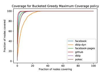
Figure 1. Coverage curve for the BGMC policy for $\tau=4$.

After obtaining the bipartite graph which has one of its sides known to us, and the other is to be predicted, we fit the following algorithms to predict the peripheral user labels

• Collaborative Filtering (via the core). We use a simple collaborative-filtering-based approach as a baseline: The labels are propagated from the core nodes to the peripheral nodes, and for each peripheral node the probability that a specific label is 1 is equal to the sample mean of the core nodes she is following. The reason for including this baseline – which is equivalent to the initialization step of NNIM (before the NNIM_Inference method) – is because we want to measure the positive contribution of the NNIM procedure – which does a kind of “sophisticated smoothing” – compared to a static one.

• Opinion Dynamics Models. Each peripheral user gets the sample mean of the influencers she’s following and then updates her vector using an update rule. We refer to two methods. The former one, NNIM (our proposed method) uses the $k$ Nearest Neighbors of each user (including herself) and aggregates the result for the next iteration according to (4). The latter is the Random HK model of (Fotakis et al., 2016) where each agent chooses a random subset of size $k$ from a set of neighbors that are contained in a certain radius $\varepsilon$. For NNIM we experiment with $k\in\{\lceil\log n\rceil,\lceil\sqrt{n}\rceil\}$ with (and without) regularization. In the case of regularization we extra static opinions at each iteration with some weight parameter $\alpha$. In our case, we add the sample mean from the influencers, which the particular user is following, at each iteration. This regularization scheme bears a resemblance to the notion of close-minded agents in (Chazelle, 2011; Chazelle and Wang, 2016). We use LSH to (approximately) construct the $k$ nearest neighbor sets efficiently. Additionally, to avoid dealing with high dimensionality prior to running the Inference_nnim procedure, we perform dimensionality reduction (PCA) keeping a 95% of the explained variance. After running the algorithm, we invert the transformation and clip the variables that fall outside $[0,1]$. For Random HK, we perform experiments with $k=\lceil\log n\rceil$ and $\varepsilon=\sqrt{d/2}$.

• Node Embeddings. We train node2vec (Grover and Leskovec, 2016), GraphWave (Donnat et al., 2018) and NodeSketch (Yang et al., 2019) embeddings on the same graph and then fit a multilabel logistic regression model. We chose node2vec as a classical random-walk-based approach, GraphWave as a transformation-based approach, and NodeSketch which is a new method based on recursive sketching.

For completeness, we also compare with the following off-the-shelf methods applied with knowledge of the whole network in order to measure – up to some extent – the effect of the network

• Label Propagation. We run the label propagation algorithm of (Raghavan et al., 2007) where initially the core nodes have labels.

• Collaborative Filtering (Dynamic). The algorithm is similar to (Raghavan et al., 2007): Instead of using the max frequency label at each iteration for each user, we take a mean of the labels of the properly labeled neighbors. Initially, only the core node have labels. This approach is also referred in (De Groot and Steg, 2009).

At this stage we have a ground truth matrix of size $|U|\times d$ with binary entries, each of which representing a whether or not each label is present in each peripheral user, and a $|U|\times d$ matrix with entries in $[0,1]$ that correspond to the predicted probabilities that each peripheral user will have a certain label present to her vector. We focus on the following metrics to quantify our findings

• AUC-ROC. We use AUC-ROC to argue about the quality of our predictions as a ranking. he AUC-ROC measure is that is serves as a metric for a bipartite ranking, that is the AUC-ROC is higher when positive labels (in the ground truth) are ranked above negative labels in terms of the attributes probabilities.. We measure the micro-averaged AUC-ROC between the two matrices (ground truth and predictions). We measure AUC-ROC in the following occasions: Between all the labels of the two matrices, and between the top 50% prevalent labels of the ground truth. We believe that these measurements reflect multiple occasions of ranking that we want to perform since, for instance, when recommending items/labels to users, we want to have a good ranking for a percentile of the labels. Furthermore, we avoid measuring the AUC-ROC in “degenerate” settings, where, for example, having some labels equal to 0 for a large percentage of the users yields a very high AUC-ROC due to negative labels being placed correctly; which is of course not representative of the reality, since positive labels may be misplaced, even at the presence of a high enough AUC-ROC.

• $F_{1}$-Score. For the Label Propagation experiment, since all outcomes are binary, we report the micro $F_{1}$-Score.

• RMSE. We perform a row-wise mean operation on the ground truth and the predicted matrices and obtain two $d$-dimensional vectors that represent the macroscopic distribution (i.e. the distribution vector across all users), and calculate the RMSE between these two vectors. Here, the RMSE metric is used to quantify the accuracy of each experiment (closeness of predictions to ground truth). The row-wise mean is performed in order to transform the two quantities to the same domain, i.e. $[0,1]^{d}$ instead of $\{0,1\}^{|U|\times d}$ and $[0,1]^{|U|\times d}$.

• Running Time. We measure the running time in seconds to demonstrate the scaling of the largest dataset (pokec). The running time of the smaller datasets is omitted, since there is no clear winner in terms of running time.

• Coverage & Influencers Core Size. We report the core size as a percentage of the total size of the network and the number of covered nodes (by the core users) w.r.t. the size of the network.

4. Discussion, Impact & Conclusion

Regarding baselines, the baselines on the entire network (Collaborative Filtering (Dynamic) and Label Propagation) yield poor results compared to the other methods. More importantly, there is even large deviation compared to the Collaborative Filtering benchmark on the bipartite graph between the core and the peripheral users, perhaps, due to highly correlated interests, which result in poorer estimations of the scores. Furthermore, the interests from the core users only, are very good starting points for estimation of the interest distributions. One possible explanation of this accords with the idea of influential users in a network who have strong opinions and tend to have uncorrelated interests with respect to the other core users, such as in the case of two strongly opinionated presidential candidates. Hence they serve as good initialization points for the initialization of NNIM. The NNIM then serves as a simulator of the peripheral interactions of users based on highly homophilic interactions, and improves both AUC-ROC and RMSE, via performing a “smoothing” procedure. Also, in fb-pages, collaborative filtering from the core users produces very good results, comparable to our method, because the page categories (politicians, governmental organizations, television shows, companies) are initially well-separated, therefore, the initial estimation step produces good estimates, since features are almost orthogonal. However, in the other datasets, where the components of the bipartite graph are not well separated and the dimensionality is higher, NNIM surpasses the baseline.

Regarding node embeddings, we report decent results in terms of AUC-ROC and RMSE in all of our experiments: In the facebook dataset we have the best performance in terms of RMSE and have AUC near the other methods; less than 1% for all labels, and similar results for top-50% and top-1. In the dblp-dyn, fb-pages and github dataset we outperform the other methods — with the exception of the AUC-ROC in top-50% in dblp-dyn where we have a 4% percent decrease. Moreover, in the fb-pages dataset, GraphWave achieves a very small RMSE however it yields a low AUC-ROC by far. In the pokec network, GraphWave and Random HK fail to run subject to our resources. Moreover, the NNIM model runs two orders of magnitude faster with $k=\lceil\log n\rceil$ neighbors and one order of magnitude faster with $k=\lceil\sqrt{n}\rceil$ neighbors compared to node2vec and NodeSketch. The PCA step does not affect the runtime considerably needing only 1 sec since it fits only on the highly influential nodes that are $n^{0.7}$, which account for 1.92% of the network. We achieve an AUC-ROC of 91.84% and an RMSE of 0.025 where we surpass NodeSketch in terms of RMSE (6 times lower) and are surpassed in terms of AUC-ROC by 0.3%. Finally, node2vec has a higher AUC-ROC rate (by a small margin) compared to NNIM with $k=\lceil\sqrt{n}\rceil$ neighbors.

The core-periphery structure of networks is a well-studied problem, but it has gathered limited attention regarding its algorithmic implications. A sublinear-size core can be in general used to speed up algorithms in ML and network science. The idea is to augment fast computation performed in the (sublinear) core, to augmentation in the periphery, which can in general extended in problems regarding community detection, embedding generation shortest paths computation etc, which in general attempts to surpass the bottleneck that the periphery cannot be easily gathered.

In this work, we present a specific application of the framework and benefit from the core-periphery structure of OSN and develop inference algorithms for interest prediction using partial information from the core users. We use the core users as initializers of a homophily-inspired evolutionary process between the peripheral users that exchanges opinions according to $k$ nearest neighbors. Our algorithm for inference is computationally efficient and has connections to traditional models, such as the HK. We prove that our algorithm converges in finite time and strictly bound the total variation distance from the consensus state. Our method is compared with others and in networks of various sizes and is capable of performing considerably faster with similar and most of the times better results. Another interesting pathway for future work is modifying the current algorithm for identifying the core in an online manner; where we maintain a priority queue where users are ordered according to their in-degree and at each iteration the user with the largest in-degree is dequeued.

Closing, the theoretical contributions by themselves do not present any foreseeable socio-economical consequences. From a practical aspect, finding the influencers in a network in terms of their structural properties and them to devise the interests of the rest of the network may have socio-economical consequences. Data provided by these users is usually public (for profit reasons) and thus core users can be used as trend-initializers. However, inferring the interests of peripheral users by using information in a semi-supervised manner may not be fairly used by external agents.

Table 2. Experiments with $p=0.7$, $\gamma=2$, $D=10^{-3}$, $\tau=4$, 10 Trees for LSH and regularization with $\alpha=1$. Random Seed = 17. The hyperparameters used for the other experiments are as follows: (a) Random HK: $D=10^{-3},\;\varepsilon=\sqrt{d/2}$; (b) node2vec: $d_{emb}=128$; (c) GraphWave: 200 samples, step size of 0.1, heat coeff. 1.0; (d) NodeSketch: $d_{emb}=32$, 2 iter.

	facebook	dblp-dyn	fb-pages	github	dblp	pokec	Running Time (s)
	AUC-ROC (all labels)
Collaborative Filtering (Dynamic)	76.61	66.59	70.83	59.91	72.5	$\dagger$	$\dagger$
Collaborative Filtering (Bipartite graph)	79.51	81.13	91.74	67.85	77.61	74.75	$\sim{10^{1}}$
node2vec	86.35	87.42	84.00	67.23	69.80	96.93	$\sim 10^{3}$
GraphWave	86.20	86.78	70.96	45.13	69.57	$\dagger$	$\dagger$
NodeSketch	80.90	81.90	68.68	49.96	58.88	92.14	$\sim 10^{3}$
Random HK ($k=\lceil\log n\rceil$)	85.75	86.30	71.90	50.34	68.83	$\dagger$	$\dagger$
NNIM ($k=\lceil\log n\rceil$)	84.24	88.05	91.86	68.07	78.64	85.60	$\sim{10^{1}}$
NNIM ($k=\lceil\sqrt{n}\rceil$)	85.82	91.16	91.62	67.86	81.65	91.84	$\sim 10^{2}$
NNIM w/ Reg ($k=\lceil\log n\rceil$)	84.17	87.39	91.78	72.31	78.86	85.05	$\sim{10^{1}}$
	AUC-ROC (top 50% of labels)
Collaborative Filtering (Dynamic)	76.61	66.59	70.83	59.91	72.5	$\dagger$	$\dagger$
Collaborative Filtering (Bipartite Graph)	83.47	86.75	100	67.85	83.43	77.38	$\sim{10^{1}}$
node2vec	54.98	94.92	78.69	67.23	68.53	96.94	$\sim 10^{3}$
GraphWave	53.97	92.91	40.11	45.13	65.70	$\dagger$	$\dagger$
NodeSketch	55.91	92.37	46.50	49.96	58.13	92.14	$\sim 10^{3}$
Random HK ($k=\lceil\log n\rceil$)	52.82	93.10	56.14	50.34	64.49	$\dagger$	$\dagger$
NNIM ($k=\lceil\log n\rceil$)	59.08	79.32	89.00	68.27	78.69	85.80	$\sim{10^{1}}$
NNIM ($k=\lceil\sqrt{n}\rceil$)	58.30	90.59	88.04	67.86	80.85	91.84	$\sim 10^{2}$
NNIM w/ Reg ($k=\lceil\log n\rceil$)	59.20	81.11	88.65	72.31	79.10	85.05	$\sim{10^{1}}$
	$F_{1}$-Score (binary predictors)
Label Propagation	30.03	52.93	90.00	87.85	48.49	34.56	$\sim 10^{1}$
	RMSE (all labels)
Collaborative Filtering (Dynamic)	0.011	0.038	0.153	0.445	0.066	$\dagger$	$\dagger$
Collaborative Filtering (Bipartite Graph)	0.012	0.067	4e-17	0.389	0.149	0.026	$\sim{10^{1}}$
node2vec	0.012	0.059	0.093	0.438	0.166	0.022	$\sim 10^{3}$
GraphWave	0.010	0.052	7e-6	0.400	0.082	$\dagger$	$\dagger$
NodeSketch	0.096	0.123	0.098	0.440	0.316	0.128	$\sim 10^{3}$
Random HK ($k=\lceil\log n\rceil$)	0.010	0.056	4e-17	0.412	0.096	$\dagger$	$\dagger$
NNIM ($k=\lceil\log n\rceil$)	0.011	0.062	4e-17	0.389	0.143	0.026	$\sim{10^{1}}$
NNIM ($k=\lceil\sqrt{n}\rceil$)	0.010	0.050	4e-17	0.388	0.128	0.025	$\sim 10^{2}$
NNIM w/ Reg ($k=\lceil\log n\rceil$)	0.012	0.066	4e-16	0.388	0.145	0.025	$\sim{10^{1}}$
Label Propagation	0.017	0.052	0.157	0.463	0.071	0.025	$\sim{10^{1}}$
Coverage (%)	88.36	97.16	72.20	68.61	66.04	51.70	—
Influencers (Core size) (%)	12.47	11.83	4.94	4.23	4.12	1.92	—
Fraction of edges in bipartite graph (%)	12.99	11.14	8.93	7.14	8.03	5.2	—

Appendix A Theoretical Properties of NNIM

Tie Breaking. We define the set $\hat{K}^{(t)}(u)$ of the $k$ nearest neighbors of $u$. In case of ties, these ties are broken arbitrarily. However, as we prove below, the relative ordering of vertices persists from one round to the next, even if ties are broken arbitrarily

Lemma 0 (Persistence of Relative Ordering).

If for two agents $u$ and $v$ at time $t_{0}$ the relation $\phi_{u}^{(t_{0})}\leq\phi_{v}^{(t_{0})}$ holds, then $\phi_{u}^{(t)}\leq\phi_{v}^{(t)}$ for all $t\geq t_{0}$ under arbitrary breaking of ties.

Proof.

Order the elements of $\hat{K}^{(t_{0})}(u)$ and $\hat{K}^{(t_{0})}(v)$ by their distance to 0. We pick the lefmost element $w\in\hat{K}^{(t_{0})}(u)$, which is related to the leftmost element $z\in K^{(t_{0})}(v)$ by the definition of $\hat{K}^{(t_{0})}(u)$ as $\phi_{w}^{(t_{0})}\leq\phi_{z}^{(t_{0})}$. We remove the two points and iterate. We finally sum the resulting inequalities and get the result for $t=t_{0}+1$. The case for every $t\geq t_{0}$ follows inductively. ∎

However, an arbitrary tie-breaking mechanism, does not guarantee that our algorithm converges. Hence, we need to devise a systematic ordering under which we resolve ties which we use to prove that our algorithm converges. A natural total ordering $\prec_{i,t}$ of the vertices is to give (globally consistent) ids to the vertices and use the ids as a secondary criterion to break ties in a unique way. The sets $K^{(t)}(u)$ of the $k$ nearest neighbors are defined with respect to the $\prec_{i,t}$ total ordering relation and therefore ties are eliminated. We also define the set $\sigma^{(t)}(u)=\{v\in U\mid\bm{\phi}_{v}^{(t)}=\bm{\phi}_{v}^{(t)}\}$. Note that $v_{j}\prec_{i,t}v_{\ell}\;\not\!\!\!\implies v_{j}\prec_{i,t+1}v_{\ell}$. Moreover, we observe that when two agents “fuse” together at time $t_{0}$, they remain fused for all $t\geq t_{0}$. The set $\sigma^{(t)}(u)$ is monotone, i.e. $t_{1}\leq t_{2}\iff\sigma^{(t_{1})}(u)\subseteq\sigma^{(t_{2})}(u)$ for all $u\in U$.

Lemma 0 (Termination).

The NNIM algorithm converges at time $T\in\mathbb{N}\cup\{\infty\}$ if and only if $|\sigma^{(T)}(u)|\geq k$ for every $u\in U$.

Proof.

$(\impliedby)$ This direction is trivial. Let $|\sigma^{(T)}(u)|\geq k$ for all $u\in U$. Then $\sigma^{(T)}(u)\supseteq K^{(T)}(u)$ for all $u\in U$. The result follows by applying the update rule and the definition of $\sigma^{(T)}(u)$.

$(\implies)$ Suppose that the NNIM algorithm converges. Equivalently for every $t\geq T$ and for every $w\in U$ we have $\phi_{w}^{(t)}=\phi_{w}^{(T)}$. We reside in the case that $t=T+1$ since the rest follows by induction. Suppose that there exists some $u\in U$ such that $|\sigma^{(T)}(u)|<k$. Then the set $K^{(T)}(u)\setminus\sigma^{(T)}(u)$ is non-empty. So $\phi_{u}^{(T+1)}=\frac{k-|K^{(T)}(u)\setminus\sigma^{(T)}(u)|}{k}\phi_{u}^{(T)}+\frac{1}{k}\sum_{w\in K^{(T)}(u)\setminus\sigma^{(T)}(u)}\phi_{v}^{(T)}$

From the fact that the system has converged we obtain that $\phi_{u}^{(T)}=\frac{1}{|K^{(T)}(u)\setminus\sigma^{(T)}(u)|}\sum_{w\in K^{(T)}(u)\setminus\sigma^{(T)}(u)}\phi_{v}^{(T)}$ which yields a contradiction since there are no constraints on the values of $\phi_{v}^{(T)}$ which impose such a relation. Therefore, for every $w\in U$ the set $\sigma^{(T)}(w)$ contains at least $k$ elements.

∎

We define the distance of two sets $W,Z\subseteq U$ as the quantity $\delta_{WZ}^{(t)}=\min_{w\in W,z\in Z}\|\phi_{w}^{(t)}-\phi_{z}^{(t)}\|$, which satisfies the properties of a metric (non-negativity, identity, symmetry, subadditivity). Moreover we define that two (non-overlapping) intervals split if and only if the $k$-nearest neighbor of each of the closest points are less than $\delta_{WZ}^{(t)}$ for some $t\geq 0$.

Lemma 0.

If two non-overlapping intervals split at $t_{0}$ then they remain split for all $t\geq t_{0}$.

Proof.

Let $W,Z\subseteq U$ be two non-overlapping clusters that have split at $t_{0}$. Let $\hat{w},\hat{z}$ be the closest points of $W,Z$. Without loss of generality let $\phi_{\hat{w}}^{(t_{0})}<\phi_{\hat{z}}^{(t_{0})}$. Then for all $u\in K^{(t_{0})}(w)$ we have that $\phi_{u}^{(t_{0})}\leq\phi_{\hat{w}}^{(t_{0})}$. By summing up we get $\phi_{\hat{w}}^{(t_{0}+1)}\leq\phi_{\hat{w}}^{(t_{0})}$. Similarly $\phi_{\hat{z}}^{(t_{0})}\leq\phi_{\hat{z}}^{(t_{0}+1)}$. Therefore the minimum distance increases. Hence the sets remain split at $t_{0}+1$. Inductively the sets remain split for all $t\geq t_{0}$ ∎

We define the splitting time of $W$ and $Z$ as the minimum $t_{0}$ that the split occurs. We also define that a subset of (consecutive) agents $W\subseteq U$ of cardinality at least $k$ is said to be isolated if and only if there exists some $t_{0}\geq 0$ such that it splits from the left set $l(W)=\{v\in U\setminus W|\phi_{v}^{(t_{0})}<\inf_{w\in W}\phi_{w}^{(t_{0})}\}$ and the right set $r(W)=\{v\in U\setminus W|\phi_{v}^{(t_{0})}>\sup_{w\in W}\phi_{w}^{(t_{0})}\}$.

Model Convergence. We now write the system in vector format $\Phi(t+1)=A(t)\Phi(t)$ where $\Phi(t)$ is the column vector with elements $\phi_{u}(t)$ and $A(t)$ is the stochastic matrix with entries $A_{uv}(t)=0$ if $v\not\in K^{(t)}(u)$ and $A_{uv}(t)=1/k$ otherwise. We use the following

Theorem 4 (Theorem 1 of (Nedić and Touri, 2012)).

Let $\{A(t)\}$ be a sequence of stochastic matrices such that the following two properties hold: (i) There exists a scalar $\gamma\in(0,1]$ such that $A_{ii}\geq\gamma$ for all $i\in[n],t\geq 0$; (ii) There exists $\alpha\in(0,1]$ s.t. $\forall\emptyset\neq S\subset[n]$ and $\bar{S}=[n]\setminus S$ it holds that $\sum_{i\in S,j\in\bar{S}}A_{ij}(t)\geq\alpha\sum_{j\in\bar{S},i\in S}A_{ji}(t)$ for all $t\geq 0$. Then the dynamics $\Phi(t+1)=A(t)\Phi(t)$ admit an adjoint sequence with probability vectors which are uniformly bounded away from 0.

We prove that our model is globally asymptotically stable (GAS).

Lemma 0 (GAS).

The NNIM model is GAS.

Proof.

We have that $A_{uu}(t)=\frac{1}{k}$, and for every element of $A(t)$ we have that $A_{uv}(t)=\frac{1}{k}\mathbf{1}\{v\in K^{(t)}(u)\}\geq\frac{1}{nk}\mathbf{1}\{u\in K^{(t)}(v)\}=\frac{1}{n}A_{vu}(t)$. Therefore, by summation on a subset $S\subset U$ we get $\sum_{u\in S,v\in\bar{S}}A_{uv}(t)\geq\frac{1}{n}\sum_{u\in\bar{S},v\in S}A_{vu}(t)$. From Theorem 4, the NNIM dynamics admit an adjoint sequence $\Pi(t)=(\pi_{1}(t),\dots,\pi_{n}(t))^{T}$ such that $\Pi^{T}(t+1)=\Pi^{T}(t)A(t)$ with $\pi_{u}(t)>p$ for all $u$ and some $1>p>0$.

We then define the Lyapunov function $V(t)=\sum_{i=1}^{n}\pi_{u}(t)\|\phi_{u}(t)-\Pi^{T}(t)\Phi(t)\|_{2}^{2}$. Our approach follows the methodology presented in (Touri, 2012) and (Nedić and Touri, 2012). Note that $V(t)\geq 0$ for all $t\geq 0$. Letting $H(t)=A^{T}(t)\mathrm{diag}(\pi_{u}(t+1))A(t)$ and doing the matrix operations expressing $V(t)$ as a quadratic form the function $V(t)$ can be written as $V(t)=V(t+1)+\frac{1}{2}\sum_{u,v}H_{uv}(t)(\phi_{u}^{(t)}-\phi_{v}^{(t)})^{2}$ since $H^{T}(t)=H(t)$. The elements of $H(t)$ are $H_{uv}(t)=\frac{1}{k^{2}}\sum_{w}\pi_{w}(t+1)\mathbf{1}\{u\in K^{(t)}w\}\mathbf{1}\{v\in K^{(t)}(w)\}$. Therefore, combining everything we arrive at

(5) $$\small V(t+1)=V(t)-\frac{1}{2k^{2}}\sum_{w}\pi_{w}(t+1)\sum_{u,v\in K^{(t)}(w)}(\phi_{u}^{(t)}-\phi_{v}^{(t)})^{2}\leq V(t)$$

Hence the function $V(t)$ is decreasing globally in $[0,1]^{d}$. Therefore $\lim_{t\to\infty}\Phi(t)=\Phi^{*}$ (non-infinite).

∎

We proceed by proving that convergence indeed occurs in finite time.

Lemma 0.

The NNIM Model converges in finite time.

Proof.

Eliminating recurrence via observing that the sum telescopes, we arrive at

(6) $$V(t)=V(0)-\frac{1}{2k^{2}}\sum_{t=0}^{T}\sum_{w}\pi_{w}(t+1)\sum_{u,v\in K^{(t)}(w)}(\phi_{u}^{(t)}-\phi_{v}^{(t)})^{2}$$

Since $V(t)\geq 0$ for every $T$, the negative difference term should vanish as $T\to\infty$. More specifically

(7) $$\lim_{T\to\infty}\frac{1}{2k^{2}}\sum_{t=0}^{T}\sum_{w}\pi_{w}(t+1)\sum_{u,v\in K^{(t)}(w))}(\phi_{u}^{(t)}-\phi_{v}^{(t)})^{2}=0$$

Note that $\pi_{w}(t+1)>p$ for some $p\in(0,1)$ by the definition of the adjoint dynamics and $k>0$, hence we have a sum of squares with positive coefficients vanishing as $T\to\infty$. In order for this to happen, every individual term of the sum must go to 0. Therefore, for every $w\in U$, by the squeeze theorem $\lim_{T\to\infty}\sum_{u,v\in K^{(T)}(w)\setminus\sigma^{(T)}(w)}(\phi_{u}^{(T)}-\phi_{v}^{(T)})^{2}=0$. Again by the same argument for all $u,v\in\lim_{T\to\infty}K^{(T)}(w)$ for all $w\in U$ we have that $\lim_{T\to\infty}(\phi_{u}^{(T)}-\phi_{v}^{(T)})=0$. By the definition of NNIM, the update process is continuous hence $\lim_{T\to\infty}\phi_{u}^{(T)}=\lim_{T\to\infty}\phi_{v}^{(T)}$ as well as by the monotonicity of $V(t)$ we know that there exists some $\phi_{w}^{*}\in[0,1]$ such that $\lim_{T\to\infty}\phi_{u}^{(T)}=\lim_{T\to\infty}\phi_{v}^{(T)}=\phi_{w}^{*}$. Hence $\lim_{T\to\infty}\phi_{u}^{(T)}=\phi_{w}^{*}$ for all $u\in\lim_{T\to\infty}K^{(T)}(w)$. Therefore for every $\epsilon_{w}>0$ there exists some $T_{w}\geq 0$ such that for all $t\geq T_{w}$ and for all $u\in K^{(t)}(w)$ we get that $|\phi_{u}^{(t)}-\phi_{w}^{*}|<\epsilon_{w}$. Now we prove finite time convergence via choosing the correct values for the $\epsilon$’s.

By Lemma 7 we know that if there exists a unique limiting point then it must be exactly approached in finite time. Suppose that there are $r\geq 2$ distinct limiting points $0\leq\phi^{*}_{1}<\phi^{*}_{2}<\dots<\phi^{*}_{r}\leq 1$. Now, fix $\epsilon>0$. We know that for every $w\in U$ and $\epsilon_{w}=\epsilon$ there exists some finite $T_{w}\geq 0$ at which $w$ reaches its limiting point within a distance of $\epsilon$. Hence the maximum distance between two elements of $K^{(t)}(w)$ for $t\geq T_{w}$ is at most $2\epsilon$, by the triangle inequality, and the same applies for every pair of points that approach this limit. Let $W_{1},\dots,W_{r}\subseteq U$ be the subsets of $U$ that approach their corresponding limits. From Theorem 1 these sets must contain consecutive agents. In order for finite convergence to occur we must impose a value of $\epsilon$ which splits the sets from each other. In this way, as we proved in Lemmas 7 and 3, we attain a finite convergence time.

First of all, let $T^{\prime}=\max_{1\leq m\leq r}\max_{w\in W_{m}}T_{w}<\infty$ and let $D=\min_{i,j}\delta^{(T^{\prime})}_{W_{i}W_{j}}$. A splitting occurs when the maximum distance between two points reaching the same limit, namely $2\epsilon$ is less than the minimum distance $D$, hence $2\epsilon<D$. A good choice for $\epsilon$ is the one which satisfies $2\epsilon+D<\min_{1\leq i\leq r-1}\{\phi^{*}_{i+1}-\phi^{*}_{i}\}$. Therefore, by these two conditions choosing $0<\epsilon<\frac{1}{4}\min_{1\leq i\leq r-1}\{\phi^{*}_{i+1}-\phi^{*}_{i}\}$ isolates the sets $W_{1},\dots,W_{r}$, hence by Lemma 7 there exist $T_{1},\dots,T_{r}<\infty$ at which each $W_{i}$ reaches its limit point. Now choose $T=T^{\prime}+\max_{1\leq i\leq r}T_{i}+1<\infty$ and the proof is complete.

∎

We provide the helper Lemma below

Lemma 0.

Suppose that the NNIM approaches (asymptotically) to a unique point $\phi^{*}$, namely $\lim_{t\to\infty}\Phi(t)=\phi^{*}\mathbf{1}$. Then this point must be reached in finite time.

Proof.

At least one of the leftmost point or the rightmost point must have (in order for the one limit point to exist) a neighbor with different coordinate, to their right or to their left respectively. Since the points have continuous positions with preserved ordering there exists some finite time $0\leq T<\infty$ at which they reach the same point $\phi^{*}$.

∎

Lemma 0.

The total variation distance $d_{TV}(t)$ of the 1D NNIM model decreases as $o(k^{-t/2})$ a.a.s. for $n\to\infty$ and any $k\in\mathbb{N}$. More specifically, if we fix some small $\delta\in[0,1]$, and $n=\Omega\left(\delta^{-1/\tau}\right)$ agents where $\tau=\lceil(\sqrt{k-1}+1)/2\rceil-1$ then with probability of at least $1-\delta$ the total variation distance $d_{TV}(t)=\frac{1}{2}\|\Phi(t)-\Phi^{*}\|_{1}$ decreases as $o(k^{-t/2})$.

Proof.

Let $\lambda_{2}(A(t^{\prime}))$ represent the second largest eigenvalues of the stochastic matrices $A(t^{\prime})$ and let $\lambda_{2}^{*}=\max_{0\leq t^{\prime}\leq t-1}\lambda_{2}(A(t^{\prime}))$. Then by the Perron-Frobenius Theorem the convergence rate is dominated by the second largest eigenvalue of the “slowest” matrix, i.e. $d_{TV}(t)=O\left((\lambda_{2}^{*})^{t}\right)$. We define the matrix sequence $\{B(t^{\prime})\}_{0\leq t^{\prime}\leq t-1}$ such that $B(t^{\prime})=kA(t^{\prime})$. The matrices $\{B(t^{\prime})\}_{0\leq t^{\prime}\leq t-1}$ represent the adjacency matrices of $k$-regular graphs with self-loops. Hence our problem resides in determining an upper bound on the second largest eigenvalue of a $k$-regular graph $G(t^{\prime})$. This is a well known problem in Spectral Graph Theory once conjectured by Alon (Nilli, 1991) and recently proved by Friedman in reference (Friedman, 2008). Alon-Friedman’s Theorem states that for any $0\leq t^{\prime}\leq t-1$ the following concentration bound holds $\Pr[\lambda_{2}(B(t^{\prime}))\leq 2\sqrt{k-1}+\varepsilon]\geq 1-O(n^{-\tau})$ for some fixed $\varepsilon>0$ and $\tau=\lceil(\sqrt{k-1}+1)/2\rceil-1$. Therefore $\Pr[\lambda_{2}(A(t^{\prime}))\in o(k^{-1/2})]\geq 1-O(n^{-\tau})$ and hence $\Pr[|\lambda_{2}^{*}|\in o(k^{-1/2})]\geq 1-O(n^{-\tau})$. For the total variation distance $d_{TV}(t)$ we get that $\Pr[d_{TV}(t)\in\Omega(k^{-t/2})]\leq O(n^{-\tau})$. Finally, choosing $n=\Omega\left(\delta^{-\frac{1}{\tau}}\right)$ we have that with probability of at least $1-\delta$ the total variation distance behaves as $o(k^{-t/2})$.

∎

Proof of Theorem 1. We combine the finite time convergence result of Lemma 6 and the convergence rate of Lemma 8. In the case of the $d$-dimensional model the guarantee translates to a total variation distance of $d\cdot D$.

Concentration Bound for the Hamming Distance (Proof Sketch). For two $d$-dimensional Bernoulli r.v.s $\bm{X},\bm{Y}$ with independent components and expectations $\bm{p},\bm{q}$ resp. we can apply McDiarmid’s ineq. (Doob, 1940) and the triangle ineq. to conclude w.p. at least $1-\delta$ the Hamming distance $\|\bm{X}-\bm{Y}\|$ varies no more than $d/2+O(\sqrt{dlog(1/\delta)})$ from the L2-squared distance $\|\bm{p}-\bm{q}\|$.

References

- (1)
- Acemoglu and Ozdaglar (2011) Daron Acemoglu and Asuman E. Ozdaglar. 2011. Opinion Dynamics and Learning in Social Networks. Dynamic Games and Applications 1, 1 (2011), 3–49.
- Anonymous (2020) Anonymous. 2020. NNIM Implementation. https://doi.org/10.5281/zenodo.3818033. https://doi.org/10.5281/zenodo.3818033
- Avin et al. (2017) Chen Avin, Michael Borokhovich, Zvi Lotker, and David Peleg. 2017. Distributed computing on core–periphery networks: Axiom-based design. J. Parallel and Distrib. Comput. 99 (2017), 51–67.
- Baum and Petrie (1966) Leonard E Baum and Ted Petrie. 1966. Statistical inference for probabilistic functions of finite state Markov chains. The annals of mathematical statistics 37, 6 (1966), 1554–1563.
- Benson and Kleinberg (2019) Austin Benson and Jon Kleinberg. 2019. Link Prediction in Networks with Core-Fringe Data. In The World Wide Web Conference. 94–104.
- Bhawalkar et al. (2013) Kshipra Bhawalkar, Sreenivas Gollapudi, and Kamesh Munagala. 2013. Coevolutionary opinion formation games. In Proc. of the 45th ACM Symposium on Theory of Computing Conference (STOC 2013). ACM, 41–50.
- Bindel et al. (2015) David Bindel, Jon Kleinberg, and Sigal Oren. 2015. How bad is forming your own opinion? Games and Economic Behavior 92 (2015), 248–265.
- Bonato et al. (2010) Anthony Bonato, Jeannette Janssen, and Pawel Prałat. 2010. The geometric protean model for on-line social networks. In International Workshop on Algorithms and Models for the Web-Graph. Springer, 110–121.
- Bonato et al. (2012) Anthony Bonato, Jeannette Janssen, and Paweł Prałat. 2012. Geometric protean graphs. Internet Mathematics 8, 1-2 (2012), 2–28.
- Bonato et al. (2015) Anthony Bonato, Marc Lozier, Dieter Mitsche, Xavier Pérez-Giménez, and Paweł Prałat. 2015. The domination number of on-line social networks and random geometric graphs. In International Conference on Theory and Applications of Models of Computation. Springer, 150–163.
- Chazelle (2011) Bernard Chazelle. 2011. The total -energy of a multiagent system. SIAM Journal on Control and Optimization 49, 4 (2011), 1680–1706.
- Chazelle and Wang (2016) Bernard Chazelle and Chu Wang. 2016. Inertial Hegselmann-Krause systems. IEEE Trans. Automat. Control 62, 8 (2016), 3905–3913.
- Chazelle and Wang (2019) Bernard Chazelle and Chu Wang. 2019. Iterated Learning in Dynamic Social Networks. Journal of Machine Learning Research 20 (2019), 29:1–29:28.
- Danescu-Niculescu-Mizil et al. (2009) Cristian Danescu-Niculescu-Mizil, Gueorgi Kossinets, Jon M. Kleinberg, and Lillian Lee. 2009. How opinions are received by online communities: a case study on amazon.com helpfulness votes. In Proceedings of the 18th International Conference on World Wide Web, (WWW 2009). ACM, 141–150.
- De et al. (2016) Abir De, Isabel Valera, Niloy Ganguly, Sourangshu Bhattacharya, and Manuel Gomez-Rodriguez. 2016. Learning and Forecasting Opinion Dynamics in Social Networks. In Advances in Neural Information Processing Systems 29: Annual Conference on Neural Information Processing Systems 2016. 397–405.
- De Groot and Steg (2009) Judith IM De Groot and Linda Steg. 2009. Morality and prosocial behavior: The role of awareness, responsibility, and norms in the norm activation model. The Journal of social psychology 149, 4 (2009), 425–449.
- Dempster et al. (1977) Arthur P Dempster, Nan M Laird, and Donald B Rubin. 1977. Maximum likelihood from incomplete data via the EM algorithm. Journal of the Royal Statistical Society: Series B (Methodological) 39, 1 (1977), 1–22.
- Desmier et al. (2012) Elise Desmier, Marc Plantevit, Céline Robardet, and Jean-François Boulicaut. 2012. Cohesive co-evolution patterns in dynamic attributed graphs. In International Conference on Discovery Science. Springer, 110–124.
- Donnat et al. (2018) Claire Donnat, Marinka Zitnik, David Hallac, and Jure Leskovec. 2018. Learning structural node embeddings via diffusion wavelets. In Proceedings of the 24th ACM SIGKDD International Conference on Knowledge Discovery & Data Mining. 1320–1329.
- Doob (1940) Joseph L Doob. 1940. Regularity properties of certain families of chance variables. Trans. Amer. Math. Soc. 47, 3 (1940), 455–486.
- Feige (1998) Uriel Feige. 1998. A threshold of ln n for approximating set cover. Journal of the ACM (JACM) 45, 4 (1998), 634–652.
- Fotakis et al. (2016) Dimitris Fotakis, Dimitris Palyvos-Giannas, and Stratis Skoulakis. 2016. Opinion Dynamics with Local Interactions.. In IJCAI. 279–285.
- Freberg et al. (2011) Karen Freberg, Kristin Graham, Karen McGaughey, and Laura A Freberg. 2011. Who are the social media influencers? A study of public perceptions of personality. Public Relations Review 37, 1 (2011), 90–92.
- Friedkin and Johnsen (1990) Noah E Friedkin and Eugene C Johnsen. 1990. Social influence and opinions. Journal of Mathematical Sociology 15, 3-4 (1990), 193–206.
- Friedman (2008) Joel Friedman. 2008. A proof of Alon’s second eigenvalue conjecture and related problems. American Mathematical Soc.
- Gaitonde et al. (2020) Jason Gaitonde, Jon M. Kleinberg, and Éva Tardos. 2020. Adversarial Perturbations of Opinion Dynamics in Networks. In EC ’20: The 21st ACM Conference on Economics and Computation. ACM, 471–472.
- Gionis et al. (1999) Aristides Gionis, Piotr Indyk, Rajeev Motwani, et al. 1999. Similarity search in high dimensions via hashing. In Vldb, Vol. 99. 518–529.
- Grover and Leskovec (2016) Aditya Grover and Jure Leskovec. 2016. node2vec: Scalable feature learning for networks. In Proceedings of the 22nd ACM SIGKDD international conference on Knowledge discovery and data mining. ACM, 855–864.
- Hamilton et al. (2017) Will Hamilton, Zhitao Ying, and Jure Leskovec. 2017. Inductive representation learning on large graphs. In Advances in neural information processing systems. 1024–1034.
- Hegselmann et al. (2002) Rainer Hegselmann, Ulrich Krause, et al. 2002. Opinion dynamics and bounded confidence models, analysis, and simulation. Journal of artificial societies and social simulation 5, 3 (2002).
- Hoffman et al. (2013) Matthew D Hoffman, David M Blei, Chong Wang, and John Paisley. 2013. Stochastic variational inference. The Journal of Machine Learning Research 14, 1 (2013), 1303–1347.
- Jia and Benson (2019) Junteng Jia and Austin R Benson. 2019. Random spatial network models for core-periphery structure. In Proceedings of the Twelfth ACM International Conference on Web Search and Data Mining. ACM, 366–374.
- Kadanoff (2009) Leo P Kadanoff. 2009. More is the same; phase transitions and mean field theories. Journal of Statistical Physics 137, 5-6 (2009), 777.
- Khamis et al. (2017) Susie Khamis, Lawrence Ang, and Raymond Welling. 2017. Self-branding,‘micro-celebrity’and the rise of Social Media Influencers. Celebrity studies 8, 2 (2017), 191–208.
- Kim and Leskovec (2011) Myunghwan Kim and Jure Leskovec. 2011. Modeling Social Networks with Node Attributes Using the Multiplicative Attribute Graph Model. In Proceedings of the Twenty-Seventh Conference on Uncertainty in Artificial Intelligence (Barcelona, Spain) (UAI’11). AUAI Press, Arlington, Virginia, USA, 400–409.
- Kim and Leskovec (2012) Myunghwan Kim and Jure Leskovec. 2012. Multiplicative attribute graph model of real-world networks. Internet mathematics 8, 1-2 (2012), 113–160.
- Krugman (1991) Paul Krugman. 1991. Increasing returns and economic geography. Journal of political economy 99, 3 (1991), 483–499.
- Leskovec and Krevl (2014) Jure Leskovec and Andrej Krevl. 2014. SNAP Datasets: Stanford Large Network Dataset Collection. http://snap.stanford.edu/data.
- Leskovec and Mcauley (2012) Jure Leskovec and Julian J Mcauley. 2012. Learning to discover social circles in ego networks. In Advances in neural information processing systems. 539–547.
- Liben-Nowell and Kleinberg (2007) David Liben-Nowell and Jon Kleinberg. 2007. The link-prediction problem for social networks. Journal of the American society for information science and technology 58, 7 (2007), 1019–1031.
- MacCormack (2010) Alan MacCormack. 2010. THE ARCHITECTURE OF COMPLEX SYSTEMS: DO" CORE-PERIPHERY" STRUCTURES DOMINATE?. In Academy of Management Proceedings, Vol. 2010. Academy of Management Briarcliff Manor, NY 10510, 1–6.
- McPherson and Ranger-Moore (1991) J Miller McPherson and James R Ranger-Moore. 1991. Evolution on a dancing landscape: organizations and networks in dynamic Blau space. Social Forces 70, 1 (1991), 19–42.
- McPherson (1983) Miller McPherson. 1983. An ecology of affiliation. American Sociological Review (1983), 519–532.
- Molavi et al. (2016) Pooya Molavi, Ceyhun Eksin, Alejandro Ribeiro, and Ali Jadbabaie. 2016. Learning to Coordinate in Social Networks. Operations Research 64, 3 (2016), 605–621.
- Molnár Jr et al. (2014) F Molnár Jr, Noemi Derzsy, Éva Czabarka, L Székely, Boleslaw K Szymanski, and Gyorgy Korniss. 2014. Dominating scale-free networks using generalized probabilistic methods. Scientific reports 4 (2014), 6308.
- Nedić and Touri (2012) Angelia Nedić and Behrouz Touri. 2012. Multi-dimensional hegselmann-krause dynamics. In 2012 IEEE 51st IEEE Conference on Decision and Control (CDC). IEEE, 68–73.
- Nemeth and Smith (1985) Roger J Nemeth and David A Smith. 1985. International trade and world-system structure: A multiple network analysis. Review (Fernand Braudel Center) 8, 4 (1985), 517–560.
- Nemhauser et al. (1978) George L Nemhauser, Laurence A Wolsey, and Marshall L Fisher. 1978. An analysis of approximations for maximizing submodular set functions—I. Mathematical programming 14, 1 (1978), 265–294.
- Nilli (1991) Alon Nilli. 1991. On the second eigenvalue of a graph. Discrete Mathematics 91, 2 (1991), 207–210.
- Papachristou (2021) Marios Papachristou. 2021. Sublinear Domination and Core-Periphery Networks. Scientific Reports (to appear) (2021).
- Pareto (1935) Vilfredo Pareto. 1935. The mind and society. Vol. 1. Harcourt, Brace and Howe.
- Perozzi et al. (2014) Bryan Perozzi, Rami Al-Rfou, and Steven Skiena. 2014. Deepwalk: Online learning of social representations. In Proceedings of the 20th ACM SIGKDD international conference on Knowledge discovery and data mining. ACM, 701–710.
- Prado et al. (2012) Adriana Prado, Marc Plantevit, Céline Robardet, and Jean-Francois Boulicaut. 2012. Mining graph topological patterns: Finding covariations among vertex descriptors. IEEE Transactions on Knowledge and Data Engineering 25, 9 (2012), 2090–2104.
- Raghavan et al. (2007) Usha Nandini Raghavan, Réka Albert, and Soundar Kumara. 2007. Near linear time algorithm to detect community structures in large-scale networks. Physical review E 76, 3 (2007), 036106.
- Rhodes and Jones (2015) CJ Rhodes and P Jones. 2015. Inferring missing links in partially observed social networks. In OR, Defence and Security. Springer, 256–271.
- Rozemberczki et al. (2019) Benedek Rozemberczki, Carl Allen, and Rik Sarkar. 2019. Multi-scale Attributed Node Embedding. arXiv:1909.13021 [cs.LG]
- Snyder and Kick (1979) David Snyder and Edward L Kick. 1979. Structural position in the world system and economic growth, 1955-1970: A multiple-network analysis of transnational interactions. American journal of Sociology 84, 5 (1979), 1096–1126.
- Stanley (1971) HE Stanley. 1971. Mean field theory of magnetic phase transitions. Introduction to Phase Transitions and Critical Phenomena (1971).
- Takac and Zabovsky (2012) Lubos Takac and Michal Zabovsky. 2012. Data analysis in public social networks. In International scientific conference and international workshop present day trends of innovations, Vol. 1.
- Touri (2012) Behrouz Touri. 2012. Averaging Dynamics in General State Spaces. In Product of Random Stochastic Matrices and Distributed Averaging. Springer, 113–126.
- Tudisco and Higham (2019) Francesco Tudisco and Desmond J Higham. 2019. A nonlinear spectral method for core–periphery detection in networks. SIAM Journal on Mathematics of Data Science 1, 2 (2019), 269–292.
- Wallerstein (1987) Immanuel Wallerstein. 1987. World-systems analysis.
- Yang et al. (2019) Dingqi Yang, Paolo Rosso, Bin Li, and Philippe Cudre-Mauroux. 2019. NodeSketch: Highly-Efficient Graph Embeddings via Recursive Sketching. In Proceedings of the 25th ACM SIGKDD International Conference on Knowledge Discovery & Data Mining. 1162–1172.
- Yang and Leskovec (2013) Jaewon Yang and Jure Leskovec. 2013. Overlapping community detection at scale: a nonnegative matrix factorization approach. In Proceedings of the sixth ACM international conference on Web search and data mining. 587–596.
- Zhang et al. (2015) Xiao Zhang, Travis Martin, and Mark EJ Newman. 2015. Identification of core-periphery structure in networks. Physical Review E 91, 3 (2015), 032803.