Self-organized criticality in neural networks

M. I. Katsnelson¹, V. Vanchurin^2,3, T. Westerhout^1*,

Abstract

We demonstrate, both analytically and numerically, that learning dynamics of neural networks is generically attracted towards a self-organized critical state. The effect can be modeled with quartic interactions between non-trainable variables (e.g. states of neurons) and trainable variables (e.g. weight matrix). Non-trainable variables are rapidly driven towards stochastic equilibrium and trainable variables are slowly driven towards learning equilibrium described by a scale-invariant distribution on a wide range of scales. Our results suggest that the scale invariance observed in many physical and biological systems might be due to some kind of learning dynamics and support the claim that the universe might be a neural network.

 

Contents

1. 1 Introduction
2. 2 Basic mechanism
3. 3 Neural networks
4. 4 Local equilibrium
5. 5 Numerical results
6. 6 Discussion

 

1 Introduction

Many astrophysical [1], geological [2], biological [3] and even neurobiological [4] systems exhibit a remarkable property of being dynamically attracted towards self-organized critical states described by scale-invariant distributions of fluctuations. The self-organized criticality is usually attributed to slowly driven non-equilibrium dynamics of the systems with “fragile” equilibrium such as the sand-pile model [5, 6, 7, 8, 9], and it is widely believed that the phenomenon is responsible for the emergence of complexity in nature [10], including biological complexity [11]. In this paper we argue that self-organized criticality is actually an equilibrium phenomenon, but in systems which undergo a learning evolution such as artificial neural networks. A distinctive feature of learning systems is the existence of two different types of degrees of freedom: non-trainable variables that are rapidly driven towards thermodynamic equilibrium and trainable variables that are slowly driven towards learning equilibrium. As we shall see, the learning equilibrium is described by frustrated dynamics on the smallest scales of fluctuations, Gaussian distributions on the largest scales, and scale-invariant distributions on intermediate scales. In what follows, we focus on the analysis of the intermediate scales and the reader is referred to Refs. [12, 13, 14] for discussions of other regimes.

Technically, we use a recently developed approach to machine learning from the point of view of statistical physics [12, 13, 14] which describes learning as a competition between a general tendency to the entropy growth in physical systems and entropy decrease due to the decrease of information uncertainty during the learning process. Near local equilibrium, the state of the learning system can be described by small fluctuations (both Gaussian and scale-invariant) near the extremal (saddle-point) state determined by this balance, with a dominant contribution of soft modes as is well known in quantum field theory [15, 16, 17]. We show that it is the soft modes of probability distribution on intermediate scales that are responsible for the scale-invariant fluctuations and the self-organized criticality in neural networks. Keeping in mind deep formal relations between theory of machine learning and fundamental physical theories [12, 13, 14] our approach probably can explain a broad distribution of self-organized critical states in completely different systems.

The paper is organized as follows. In Sec. 2 we describe a mechanism which might be responsible for the emergence of self-organized criticality in the context of a simple model. In Sec. 3 we argue that the most essential feature of the model is also present in more general learning systems such as artificial neural networks. In Sec. 4 we show that the learning evolution of neural networks would generically lead to the emergence of self-organized critical states described by a scale-invariant distribution over trainable variables. In Sec. 5 the main results are verified numerically by following the learning dynamics of artificial neural networks with feedforward architecture. In Sec. 6 we discuss implications of the results for machine learning, physics and biology.

2 Basic mechanism

In this section we describe the basic mechanism of the self-organized criticality in the context of a simple model with one non-trainable variable $x$ and one trainable variable $q$, but, as we shall see, essentially the same mechanism is responsible for the critical behavior of neural networks with many non-trainable and trainable variables. The main objective of a learning system is to minimize some suitably defined loss function $H(x,q)$ which can be expanded around local extremum up to the second order, i.e.

$$H(x,q)\approx\frac{\lambda_{x}(x-\bar{x})^{2}}{2}+\frac{g(q-\bar{q})^{2}(x-\bar{x})^{2}}{2}+\frac{\lambda_{q}(q-\bar{q})^{2}}{2}+...$$ (1)

where $\bar{x}$ and $\bar{q}$ are mean values of $x$ and $q$ respectively, and $\lambda_{x}$, $g$ and $\lambda_{q}$ specify the coupling constants. It is explicitly assumed that there is a quartic coupling between trainable and non-trainable variable, but higher order terms might also be present. We also assume that non-trainable variable $x$ undergoes stochastic dynamics (which maximizes the entropy due to the second law of thermodynamics) and trainable variable $q$ undergoes learning dynamics (which minimizes the entropy due to the second law of learning) [12]. In the equilibrium the overall entropy remains constant, but the loss function (averaged over the non-trainable variable) depends on the trainable variable:

$$\int dx\;p(x|q)H(x,q)=U(q).$$ (2)

Then, according to the maximum entropy principle, conditional distribution $p(x|q)$ over non-trainable stochastic variable $x$ is given by

$$p(x|q)\propto\exp\left(-\frac{\beta\lambda_{x}(x-\bar{x})^{2}}{2}-\frac{\beta g(q-\bar{q})^{2}(x-\bar{x})^{2}}{2}-\frac{\beta\lambda_{q}(q-\bar{q})^{2}}{2}+...\right)$$ (3)

and the corresponding free energy is

$$F(\beta,q)\approx\frac{1}{2\beta}\log(g(q-\bar{q})^{2}+\lambda_{x})+\frac{\lambda_{q}(q-\bar{q})^{2}}{2}+\frac{1}{2\beta}\log(\beta).$$ (4)

The next step is to derive marginal distribution $p(q)$, and consequently the joint distribution $p(x,q)=p(x|q)p(q)$. If we assume that both $g$ and $\lambda_{q}$ are positive, but $\lambda_{x}$ is negative, then the local minimum of the loss function is at $q=\bar{q}$, but the maximum entropy of $p(x|q)$ is at $q=\bar{q}\pm\sqrt{-\lambda_{x}/g}$, or when the conditional distribution $p(x|q)$ is nearly flat. In the limit of small fluctuations, $|q-\bar{q}|\lesssim\sqrt{-\lambda_{x}/g}$, the dynamics of $q$ becomes frustrated: the learning dynamics pushes $q$ towards $\bar{q}$, but the stochastic dynamics pushes $q$ towards either $\bar{q}+\sqrt{-\lambda_{x}/g}$ or $\bar{q}-\sqrt{-\lambda_{x}/g}$. This is exactly the limit when the argument of the logarithm in (4) is negative, the conditional distribution $p(x|q)$ has a local maximum at $x=\bar{x}$ and higher order terms must be added to the expansion (1). Note that the frustration only happens for very small values of $(q-\bar{q})^{2}\lesssim-\lambda_{x}/g$ (or equivalently for small changes of the loss function, $H(q)\propto(q-\bar{q})^{2}$) where the quantum behavior can emerge (see Ref. [14]), and self-organized criticality is expected to emerge on larger scales $(q-\bar{q})^{2}>-\lambda_{x}/g$ (see Eq. (7)).

According to the first law of learning [12], the marginal distribution $p(q)$ must evolve towards a state described by a saddle point of the free energy. If we impose a constraint on the average free energy,

$$\int d{q}\;p(q){F}(\beta,q)=V,$$ (5)

then the equilibrium distribution is

$$p(q)\propto e^{-\alpha F({\beta},q)}\propto(g(q-\bar{q})^{2}+\lambda_{x})^{-\frac{\alpha}{2{\beta}}}\exp\left(-\frac{\alpha\lambda_{q}(q-\bar{q})^{2}}{2}\right).$$ (6)

where $\alpha$ is a Lagrange multiplier associated with the constraint (5). Evidently, for $\alpha>0$, smaller fluctuations (e.g. on shorter time-scales) would be described by a power-law (or scale-invariant) distribution and larger fluctuations (e.g. on longer time-scales) would be described by a Gaussian distribution, i.e.

$$p(q)\propto\begin{cases}(g(q-\bar{q})^{2}+\lambda_{x})^{-\frac{\alpha}{2{\beta}}}&\;\;\;\text{for}\;\;-\frac{\lambda_{x}}{g}<(q-\bar{q})^{2}<\frac{W(\beta\lambda_{q})}{\beta\lambda_{q}}\,,\\ \exp\left(-\frac{\alpha\lambda_{q}(q-\bar{q})^{2}}{2}\right)&\;\;\;\text{for}\;\;(q-\bar{q})^{2}>\frac{W(\beta\lambda_{q})}{\beta\lambda_{q}}\,,\end{cases}$$ (7)

where $W(x)$ is the Lambert W function [18]. This suggests that the presence of scale-invariant trainable variables, or, in other words, self-organized critical states, is a direct consequence of the learning dynamics on the intermediate scales, $-\lambda_{x}/g<(q-\bar{q})^{2}<W(\beta\lambda_{q})/(\beta\lambda_{q})$.

3 Neural networks

In the previous section we described a simple model with a scale-invariant distribution over trainable variables, but the learning dynamics which might lead to such a distribution was not yet specified. The key observation was that for the scale-invariance to emerge, interactions between trainable and non-trainable variables must be quartic (1). It turns out that such interactions are very typical in the context of neural networks for non-trainable states of neurons ${\bf x}$ and trainable elements of the so-called weight matrix $\hat{w}$ (see Eqs. (11) and (10)). Because of the quartic couplings, trainable elements of the weight matrix and bias vector are expected to evolve towards a scale-invariant distribution or, in other words, towards a self-organized critical state.

For numerical tests we will be mainly interested in a feedforward neural architecture (see Sec. 5), but according to analytical results (see Sec. 4) it is expected that the same phenomenon would occur in an arbitrary learning system. In general, a neural network can be defined as a septuple $({\bf x},\hat{P},p_{\partial},\hat{w},{\bf b},{\bf f},H)$, where:

1. ${\bf x}$, is a (column) state vector of all (input, output and hidden) neurons,

2. $\hat{P}$, is the boundary projection operators to subspace spanned by input/output neurons,

3. $p_{\partial}({\bf x}_{\partial})$, is a probability distribution which describes the training dataset,

4. $\hat{w}$, is a weight matrix which describes connections between neurons,

5. ${\bf b}$, is a (column) bias vector which describes bias in inputs of individual neurons,

6. ${\bf f}({\bf y})$, is an activation map which describes a non-linear part of the dynamics,

7. ${H}({\bf x},{\bf b},\hat{w})$, is a loss function which describes the learning objective.

We shall refer to all input and output neurons, described by the state vector $\hat{P}{\bf x}$, as boundary neurons, and to all neurons in the hidden layers, described by the state vector $(\hat{I}-\hat{P}){\bf x}$, as bulk neurons. These different types of neurons evolve according to two different laws (8) and (9). The state of the boundary neurons depends only on the boundary data,

$$\hat{P}{\bf x}(t)=\hat{P}{\bf x}_{\partial}(t),$$ (8)

where ${\bf x}_{\partial}(t)$ is updated either periodically or randomly from a training dataset which can be described by some probability distribution $p_{\partial}({\bf x}_{\partial})$. In contrast, the bulk neurons evolve according to

$$(\hat{I}-\hat{P}){\bf x}({t})=(\hat{I}-\hat{P}){\bf f}\left(\hat{w}{\bf x}(t-1)+{\bf b}\right),$$ (9)

where the activation map acts separately on each component, i.e. $f_{i}({\bf y})=f_{i}(y_{i})$. These functions are called activation functions (e.g. hyperbolic tangent $\tanh(y)$, rectifier linear unit function $\max(0,x)$, etc.) and do not need to be the same for all neurons.

The main problem in machine learning is to find a bias vector ${\bf b}$ and a weight matrix $\hat{w}$ which minimize (the time-$t$ average or ensemble average over boundary conditions $p_{\partial}({\bf x}_{\partial})$ of) some suitably defined quantity known as the loss function. For example, a boundary loss function could be defined as

$$H_{\partial}({\bf x},{\bf b},\hat{w}) = \frac{1}{2}\left({\bf x}-{\bf f}\left(\hat{w}{\bf x}+{\bf b}\right)\right)^{\dagger}\hat{P}\left({\bf x}-{\bf f}\left(\hat{w}{\bf x}+{\bf b}\right)\right)$$ (10)

where because of the inserted projection operator $\hat{P}$, the sum is taken over squared errors at only boundary neurons [12]. Note that in a feedforward neural architecture there are no errors associated with input neurons and all of the loss comes from the output neurons. Another example is the bulk loss function, e.g.

$$H({\bf x},{\bf b},\hat{w}) = \frac{1}{2}\left({\bf x}-{\bf f}\left(\hat{w}{\bf x}+{\bf b}\right)\right)^{\dagger}\left({\bf x}-{\bf f}\left(\hat{w}{\bf x}+{\bf b}\right)\right)+\frac{1}{2}{V}({\bf x},{\bf b},\hat{w})$$ (11)

where in addition to the first term, which represents a sum of local errors over all neurons, there may be a second term which represents either local objectives or constraints imposed by a neural architecture [12]. Note that boundary loss is usually used in supervised learning, but bulk loss functions may be used for both supervised and unsupervised learning tasks.

4 Local equilibrium

To study the learning dynamics of neural networks analytically it is convenient to switch to a more“macroscopic” description. Instead of following the individual states we shall study the dynamics of a joint distribution $p({\bf x},{\bf q})=p({\bf x}|{\bf q})p({\bf q})$ over non-trainable variables ${\bf x}$, which describe the current state vector of $N$ neurons, and trainable variables ${\bf q}$, which describe the state of $K$ dynamical elements of weight matrix ${\bf w}({\bf q})$ and bias vector ${\bf b}({\bf q})$. If we fix the trainable variables ${\bf q}$ and impose a constraint on the average loss function

$$\int d^{N}xH({\bf x},{\bf q})p({\bf x}|{\bf q})=U({\bf q}),$$ (12)

then the maximum entropy probability distribution is given by

$$p({\bf x}|{\bf q})\propto\exp\left(-\beta H({\bf x},{\bf q})\right).$$ (13)

The bulk loss function (11) can be expanded around a local extremum $(\bar{\mathbf{x}},\bar{\mathbf{q}})$ as

$$H({\bf x},{\bf q})=\frac{1}{2}({\bf x}-\bar{\bf x})^{\dagger}\left(\hat{G}({\bf q})+\hat{V}_{x}\right)({\bf x}-\bar{\bf x})+\frac{1}{2}({\bf q}-\bar{\bf q})^{\dagger}\hat{V}_{q}({\bf q}-\bar{\bf q}),$$ (14)

where

$$\hat{G}({\bf q})\equiv\left(\hat{I}-\hat{F}\hat{w}\right)^{\dagger}\left(\hat{I}-\hat{F}\hat{w}\right).$$ (15)

For simplicity we assume that $\hat{F}$, $\hat{V}_{x}$ and $\hat{V}_{q}$ are diagonal matrices of, respectively, first derivatives of activation functions $f_{i}(y_{i})$ and second derivatives of local potentials $V({\bf x},{\bf q})$ with respect to non-trainable ${\bf x}$ and trainable ${\bf q}$ variables. Then the free energy of the maximum entropy distribution (13) is given by [12],

$${F}({\beta},{\bf q})=\frac{1}{2\beta}\log\det\left(\beta\hat{G}({\bf q})+\beta\hat{V}_{x}\right)+\frac{1}{2}({\bf q}-\bar{\bf q})^{\dagger}\hat{V}_{q}({\bf q}-\bar{\bf q}).$$ (16)

The next step is to determine the marginal distribution $p({\bf q})$ and consequently the joint distribution $p({\bf x},{\bf q})=p({\bf x}|{\bf q})p({\bf q})$. If we impose a constraint on the free energy

$$\int d{\bf q}\;p({\bf q}){F}({\beta},{\bf q})=V,$$ (17)

then the marginal distribution is

$$p({\bf q})\propto\exp\left(-\alpha{F}({\beta},{\bf q})\right).$$ (18)

For free energy (16) the distribution is

$$p({\bf q})\propto\left[\det\left(\hat{G}({\bf q})+\hat{V}_{x}\right)\right]^{-\frac{\alpha}{2\beta}}\exp\left(-\frac{\alpha}{2}({\bf q}-\bar{\bf q})^{\dagger}\hat{V}_{q}({\bf q}-\bar{\bf q})\right).$$ (19)

Since in the learning equilibrium the free energy would be extremized, it makes sense to expand individual eigenvalues $\lambda_{i}({\bf q})$ of the matrix $\hat{G}({\bf q})+\hat{V}_{x}$ around local extrema,

$$\lambda^{i}({\bf q})\approx\lambda^{i}_{0}+\left({\bf q}-\bar{\bf q}\right)^{\dagger}\hat{\lambda}^{i}\left({\bf q}-\bar{\bf q}\right),$$ (20)

and then the distribution (18) can be approximated as

$$p({\bf q})\propto\prod_{i}\left(\lambda^{i}_{0}+\left({\bf q}-\bar{\bf q}\right)^{\dagger}\hat{\lambda}^{i}\left({\bf q}-\bar{\bf q}\right)\right)^{-\frac{\alpha}{2\beta}}\exp\left(-\frac{\alpha}{2}({\bf q}-\bar{\bf q})^{\dagger}\hat{V}_{q}({\bf q}-\bar{\bf q})\right).$$ (21)

Evidently, the marginal distribution $p({\bf q})$ would be scale-invariant (or a power-law) on intermediate scales when the first term dominates and Gaussian on larger scales when the second term dominates. Therefore, the scale-invariant and Gaussian distributions are expected for, respectively, short-term and long-term dynamics. Also note that for very small fluctuations (e.g. when $\left({\bf q}-\bar{\bf q}\right)^{\dagger}\hat{\lambda}^{i}\left({\bf q}-\bar{\bf q}\right)$ and $\lambda^{i}_{0}$ are of the same order but have opposite signs) the free energy (16) might diverge and the system can become frustrated from simultaneous maximization of the entropy of non-trainable variables and minimization of the entropy of trainable variables. (See Sec. 2 for a discussion of this point in the context of a simple model.)

5 Numerical results

In this section we will justify the model from Sec. 4 by training a feedforward neural network until it reaches equilibrium and then analyzing its behavior in equilibrium.

We focus on the MNIST dataset [19] which is a collection of images of handwritten digits. It contains 60000 training and 10000 test samples. We use a simple fully-connected feedforward neural network with two hidden layers with 700 and 476 neurons and ReLU [20] activation function. This network is optimized using stochastic gradient descend with batch size $1$ and learning rate $2\cdot 10^{-3}$. We also add $L_{2}$-regularization term to the loss function with rate $5\cdot 10^{-4}$. The training proceeds for $\mathcal{O}(3000)$ epochs (i.e. passes through the dataset) to reach equilibrium. We keep track of the loss function on the test dataset and ensure that no overfitting takes place.

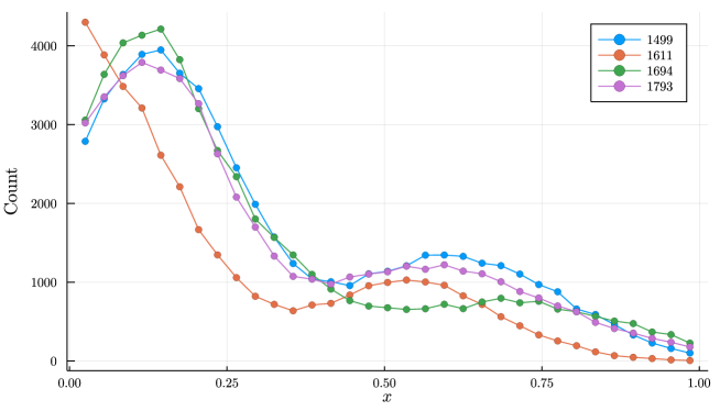
Figure 1: Output distribution $p(x|\mathbf{q})$ for a few randomly selected neurons with frozen weights (i.e. no training takes place). All neurons come from the second hidden layer.

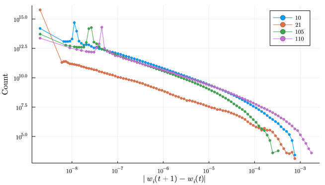
Figure 2: Distribution of local fluctuations for a few randomly selected weights from the first and second layer.

We can now directly compute $p(x|\mathbf{q})$ by freezing the neural network parameters and tracking neuron outputs for different input images. The result is shown in Figure 1. We clearly see two maxima which correspond to the frustrated regime discussed in Sec. 4. This regime is characterized by negative $\lambda^{i}_{0}$ from (20) which, because of (13), appear as local minima in $p(x|\mathbf{q})$.

Next, we train the neural network for another 200 epochs and keep track of a few randomly selected weights. As a result we have time dependence $w_{i}(t)$ of trainable parameters in equilibrium. This data can be used to gain insight into $p(\mathbf{q})$.

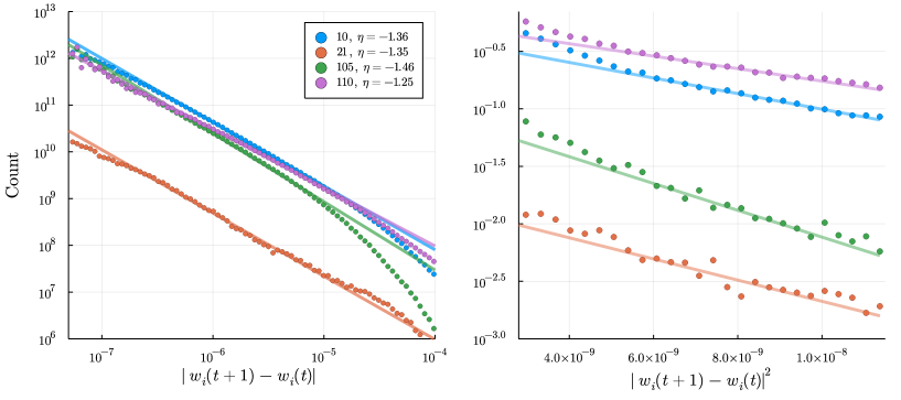
Figure 3: Distribution of local fluctuations for a few randomly selected weights. This figure contains the exact same data as Figure 2, but focuses on intermediate (left panel) and large (right panel) fluctuations. Left panel shows data in log-log scale and straight lines correspond to power-law behavior. Right panel shows data in log-quadratic scale and straight lines correspond to Gaussian decays.

In Sec. 4 we expanded everything around $\mathbf{\bar{q}}$. In reality, the situation might be more complicated because there might be many extrema close to one another such that in equilibrium the neural network constantly “hops” between them. To account for this hopping we will consider truly local fluctuations: $w_{i}(t+1)-\bar{w}_{i}(t)\approx w_{i}(t+1)-w_{i}(t)$. The distribution of these fluctuations is shown in Figure 2. We see a peak for very small fluctuations, power-law decay at intermediate values, and Gaussian decay for large fluctuations. In Figure 3 we focus on the intermediate and large fluctuations to better illustrate the power-law and Gaussian decays. This behavior matches (21) perfectly.

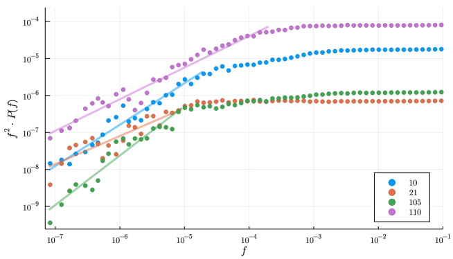
Figure 4: Power spectrum of $w_{i}(t)$. We show $f^{2}\cdot P(f)$ rather than $P(f)$ to more clearly indicate the deviations from $1/f^{2}$ behavior which is expected for completely uncorrelated jumps. Straight lines are guide to eye and indicate regions where the power spectrum decays as $1/f^{a}$ with $a<2$.

Finally, we analyze the power spectrum of $w_{i}(t)$, i.e.

$$P(f) \equiv \left|\int_{0}^{T}dtw_{i}(t)e^{-ift}\right|^{2}=\frac{1}{f^{2}}\left|\int_{0}^{T}dt\;\frac{dw_{i}(t)}{dt}e^{ift}\right|^{2}\,.$$ (22)

$\left\langle\left|\int_{0}^{T}dt\;\frac{dw_{i}(t)}{dt}e^{ift}\right|^{2}\right\rangle$ is constant for independent increments, i.e. when

$$\left\langle\frac{dw_{i}(t)}{dt}\frac{dw_{i}(z)}{dz}\right\rangle\propto\delta(t-z)$$ (23)

as would be the case, for example, for white noise. In Figure 4 we show $f^{2}\cdot P(f)$ as a function of $f$ such that $1/f^{2}$ dependence would correspond to a horizontal line. On short time scales (corresponding to large $f$) the system is in a local minimum and the dynamics of $w_{i}(t)$ can be modeled with uncorrelated jumps described by power spectrum $P(f)\propto 1/f^{2}$. On the long time scales (small $f$) the system is hopping between local minima and the jumps are are described by power spectrum $P(f)\propto 1/f^{a}$ with $a<2$. (See Refs. [12, 13, 14] for analytical modeling of the learning dynamics of $p(q,t)$ and $F(q,t)$ on both short and long time-scales.)

6 Discussion

In this article, we analyzed, both numerically and analytically, the learning dynamics of neural networks near equilibrium and showed that the learning systems are generally attracted towards critical states described by scale-invariant distributions over trainable variables on a wide range of scales. Moreover, on even larger scales the trainable degrees of freedom behave as Gaussian random variables and on somewhat smaller scales the dynamics is frustrated from simultaneous maximization of the entropy of non-trainable variables and minimization of the entropy of trainable variables. These results have some interesting implications for machine learning, physics and biology.

Machine learning. Every trainable variable evolves towards a state described by a scale-invariant distribution on a range of scales, but the range itself can be very different for different variables. Some variables are very well trained and have a scale-invariant distribution on a wide range of scales, whereas others are poorly trained and the scale-invariant range is very narrow. This suggests that the size of the range can be used to determine how well a given trainable variable was trained or how vital it is for the overall performance of the network. For example, if the least vital trainable variables (i.e. with the smallest ranges of scale-invariant distributions) can be successfully identified, then the learning algorithm can be improved or the neural network can be compressed by either rewiring or dropping the least vital connections. On a more practical level, the scale-invariant range is usually smaller for trainable variables whose amplitude of fluctuations is larger (and vise versa), and therefore the amplitude can be used to identify the least vital connections that should be either dropped (for compressing neural networks) or rewired (for improving efficiency of learning).

Physics. It was recently proposed that the entire universe may be a neural network which undergoes a learning evolution [13]. If correct, then all of the physical phenomena are not fundamental, but rather emergent, and provide an adequate description in the limit of large number of degrees of freedom, e.g. neurons, weights, biases etc. In particular, it was shown that the learning dynamics near equilibrium can be modeled using either thermodynamics [12] or quantum mechanics [14] and further away from the equilibrium using either Hamiltonian mechanics or general relativity [13]. In this paper we uncovered yet another near-equilibrium limit in which a self-organized criticality emerges on intermediate scales from the learning dynamics of neural networks. Given that the self-organized criticality is observed in many physical (and also biological) systems, our results support the claim that the entire universe may be a neural network.

Biology. Self-organized criticality in the context of biological complexity was recently discussed in Ref. [11]. It was suggested that competing interactions between different levels of organization form a universal mechanism leading to biological complexity. At the same time, mathematical mechanisms responsible for the self-organized criticality in biology [6, 9, 10] are still very poorly studied. It is a big temptation to identify, in some sense, Darwin selection with learning and apply the theory of machine learning to evolutionary biology. This exciting issue is far beyond the scope of this work and will be considered elsewhere.

Funding information

V.V. was supported in part by the Foundational Questions Institute (FQXi) and the Oak Ridge Institute for Science and Education (ORISE). The work of M.I.K. and T.W. was supported by European Research Council via Synergy Grant 854843 - FASTCORR. Numerical simulations in this work were carried out on the Dutch national e-infrastructure with the support of SURF Cooperative.

References

- [1] M. Aschwanden, Self-Organized Criticality in Astrophysics, Springer Berlin Heidelberg, ISBN 9783642150005, 9783642150012, 10.1007/978-3-642-15001-2 (2011).
- [2] R. Smalley, D. Turcotte and S. A. Solla, A renormalization group approach to the stick-slip behavior of faults, J. Geophys. Res. 90(B2), 1894 (1985), 10.1029/jb090ib02p01894.
- [3] K. Sneppen, P. Bak, H. Flyvbjerg and M. Jensen, Evolution as a self-organized critical phenomenon., Proc. Natl. Acad. Sci. 92(11), 5209 (1995), 10.1073/pnas.92.11.5209.
- [4] K. Linkenkaer-Hansen, V. V. Nikouline, J. M. Palva and R. J. Ilmoniemi, Long-range temporal correlations and scaling behavior in human brain oscillations, J. Neurosci. 21(4), 1370 (2001), 10.1523/jneurosci.21-04-01370.2001.
- [5] P. Bak, C. Tang and K. Wiesenfeld, Self-organized criticality, Phys. Rev. A 38(1), 364 (1988), 10.1103/physreva.38.364.
- [6] P. Bak and K. Sneppen, Punctuated equilibrium and criticality in a simple model of evolution, Phys. Rev. Lett. 71(24), 4083 (1993), 10.1103/physrevlett.71.4083.
- [7] S. Maslov, M. Paczuski and P. Bak, Avalanches and 1/f noise in evolution and growth models, Phys. Rev. Lett. 73(16), 2162 (1994), 10.1103/physrevlett.73.2162.
- [8] S. Maslov and Y.-C. Zhang, Exactly solved model of self-organized criticality, Phys. Rev. Lett. 75(8), 1550 (1995), 10.1103/physrevlett.75.1550.
- [9] P. Bak and M. Paczuski, Complexity, contingency, and criticality., Proc. Natl. Acad. Sci. 92(15), 6689 (1995), 10.1073/pnas.92.15.6689.
- [10] P. Bak, How Nature Works, Springer New York, ISBN 9780387987385, 9781475754261, 10.1007/978-1-4757-5426-1 (1996).
- [11] Y. I. Wolf, M. I. Katsnelson and E. V. Koonin, Physical foundations of biological complexity, Proc Natl Acad Sci USA 115(37), E8678 (2018), 10.1073/pnas.1807890115.
- [12] V. Vanchurin, Toward a theory of machine learning, Mach. Learn.: Sci. Technol. 2(3), 035012 (2021), 10.1088/2632-2153/abe6d7.
- [13] V. Vanchurin, The world as a neural network, Entropy-switz. 22(11), 1210 (2020), 10.3390/e22111210.
- [14] M. I. Katsnelson and V. Vanchurin, Emergent quantumness in neural networks, arXiv preprint arXiv:2012.05082 (2020).
- [15] S. Coleman, The uses of instantons, In The Whys of Subnuclear Physics, pp. 805–941. Springer US, ISBN 9781468409932, 9781468409918, 10.1007/978-1-4684-0991-8_16 (1979).
- [16] A. Vainshtein, V. Zakharov, V. Novikov and M. Shifman, ABC of instantons, In Instantons in Gauge Theories, pp. 468–488. WORLD SCIENTIFIC, ISBN 9789810216818, 9789812794345, 10.1142/9789812794345_0044 (1994).
- [17] R. Rajaraman, Solitons and instantons (1982).
- [18] Lambert w function, https://en.wikipedia.org/wiki/Lambert_W_function .
- [19] Y. Lecun, L. Bottou, Y. Bengio and P. Haffner, Gradient-based learning applied to document recognition, Proc. IEEE 86(11), 2278 (1998), 10.1109/5.726791.
- [20] V. Nair and G. E. Hinton, Rectified linear units improve restricted boltzmann machines, In Icml (2010).