Differentiable Architecture Pruning for Transfer Learning

Abstract

We propose a new gradient-based approach for extracting sub-architectures from a given large model. Contrarily to existing pruning methods, which are unable to disentangle the network architecture and the corresponding weights, our architecture-pruning scheme produces transferable new structures that can be successfully retrained to solve different tasks. We focus on a transfer-learning setup where architectures can be trained on a large data set but very few data points are available for fine-tuning them on new tasks. We define a new gradient-based algorithm that trains architectures of arbitrarily low complexity independently from the attached weights. Given a search space defined by an existing large neural model, we reformulate the architecture search task as a complexity-penalized subset-selection problem and solve it through a two-temperature relaxation scheme. We provide theoretical convergence guarantees and validate the proposed transfer-learning strategy on real data.

Keywords: architecture search, transfer learning, discrete optimization

1 Introduction

Motivation.

Transfer learning methods aim to produce machine learning models that are trained on a given problem but perform well also on different new tasks. The interest in transfer learning comes from situations where large data sets can be used for solving a given training task but the data associated with new tasks are too small to train expressive models from scratch. The general transfer-learning strategy is to use the small available new data for adapting a large model that has been previously optimized on the training data. One option consists of keeping the structure of the pre-trained large model intact and fine-tuning its weights to solve the new task. When very few data points are available and the pre-trained network is large, however, customized regularization strategies are needed to mitigate the risk of over-fitting. Fine-tuning only a few parameters is a possible way out but can strongly limit the performance of the final model. Another option is to prune the pre-trained model to reduce its complexity, increase transferability, and prevent overfitting. Existing strategies, however, focus on optimized models and are unable to disentangle the network architecture from the attached weights. As a consequence, the pruned version of the original model can hardly be interpreted as a transferable new architecture and it is difficult to reuse it on new tasks.

In this paper.

We propose a new Architecture Pruning (AP) approach for finding transferable and arbitrarily light sub-architectures of a given parent model. AP is not dissimilar to other existing pruning methods but based on a feasible approximation of the objective function normally used for Neural Architecture Search (NAS). We conjecture that the proposed architecture-focused objective makes it possible to separate the role of the network architecture and the weights attached to it. To validate our hypothesis, we define a new AP algorithm and use it to extract a series of low-complexity sub-architectures from state-of-the-art computer vision models with millions of parameters. The size of the obtained sub-architectures can be fixed a priori and, in the transfer learning setup, adapted to the amount of data available from the new task. Finally, we test the transferability of the obtained sub-architectures empirically by fine-tuning them on different small-size data sets.

Technical contribution.

NAS is often formulated as a nested optimization problem, e.g.

$$\min_{{\cal A}}{\cal L}\left({\cal A},\ {\rm arg}\min_{\theta}{\cal L}({\cal A},\theta,{\cal D}),\ {\cal D}\right)$$ (1)

where ${\cal L}({\cal A},\theta,{\cal D})$ is a loss function that depends on the network structure, ${\cal A}$, the corresponding weights, $\theta$, and the input-output data set, ${\cal D}$. This approach has a few practical problems: i) the architecture search space, i.e. the set of possible architectures to be considered, is ideally unbounded, ii) each new architecture, ${\cal A}^{\prime}$, should be evaluated after solving the inner optimization problem, ${\rm arg}\min_{\theta}{\cal L}({\cal A}^{\prime},\theta)$, which is computationally expensive, and iii) architectures are usually encoded as discrete variables, i.e. $\min_{{\cal A}}{\cal L}$, is a high-dimensional Discrete Optimization (DO) problem and its exact solution may require an exponentially large number of architecture evaluations. To address these issues, we approximate (1) with the joint mixed-DO problem $\min_{{\cal A},\theta}{\cal L}({\cal A},\theta)$ i.e. we simultaneously search for an optimal architecture, ${\cal A}$ and the corresponding weights, $\theta$. The DO problem is then solved through a new two-temperature gradient-based approach where a first approximation makes $\min_{{\cal A},\theta}{\cal L}({\cal A},\theta)$ a fully continuous optimization problem and a second approximation is introduced to avoid the vanishing gradient, which may prevent gradient-based iterative algorithm to converge when the first approximation is tight. Our scheme belongs to a class of recent differentiable NAS approaches, which are several orders of magnitude faster than standard Genetic and Reinforcement Learning schemes (see for example the comparative table of Ren et al. (2020)) but the first to address the vanishing-gradient problem explicitly in this framework. Similar relaxation methods have been used in the binary networks literature (see for example et al. (2013)), but this is the first time that similar ideas are transferred from the binary network literature to NAS. Moreover, our method is provably accurate and, among various existing follow-ups of et al. (2013), the only one that can be provided with quantitative convergence bounds.

We validate our hypothesis and theoretical findings through three sets of empirical experiments: i) we compare the performance of the proposed two-temperature scheme and a more standard continuous relaxation method on solving a simple AP problem (on MNIST data), ii) we use CIFAR10 and CIFAR100 to test the transferability of VGG sub-architectures obtained through AP and other pruning methods , and iii) we confirm the hypothesis of Frankle et al. (2020) that NAS can be often reduced to selecting the right layer-wise density and is quite insensitive to specific configurations of the connections.

Related Work.

NAS approaches Zoph and Le (2016); Liu et al. (2018); Gaier and Ha (2019); You et al. (2020) look for optimal neural structures in a given search space, and employ weight pruning procedures that attempt to improve the performance of large (over-parameterized) networks by removing the ‘less important’ connections. Early methods Stanley and Miikkulainen (2002); Zoph and Le (2016); Real et al. (2019) are based on expensive genetic algorithms or reinforcement learning approaches. More recent schemes either design differentiable losses Liu et al. (2018); Xie et al. (2019), or use random weights to evaluate the performance of the architecture on a validation set Gaier and Ha (2019); Pham et al. (2018). Unlike these methods, which search architectures by adding new components, our method removes redundant connections from an over-parameterized parent network. Network pruning approaches Collins and Kohli (2014); Han et al. (2015b, a, b); Frankle and Carbin (2019); Yu et al. (2019); Frankle et al. (2020) start from pre-trained neural models and prune the unimportant connections to reduce the model size and achieve better performance. Contrarily to the transfer learning goals of AP, these methods mostly focus on single-task setups. Network quantization and binarization reduce the computational cost of neural models by using lower-precision weights Jacob et al. (2018); Zhou et al. (2016), or mapping and hashing similar weights to the same value Chen et al. (2015); Hu et al. (2018). In an extreme case, the weights, and sometimes even the inputs, are binarized, with positive/negative weights mapped to $\pm 1$ Soudry et al. (2014); Courbariaux et al. (2016); Hubara et al. (2017); Shen et al. (2019); Courbariaux et al. (2015). As a result, these methods keep all original connections, i.e. do not perform any architecture search. Often used for binary network optimization, Straight-Through gradient Estimator (STE) algorithms are conceptually similar to the two-temperature scheme proposed here. STE looks at discrete variables as the output of possibly non-smooth and non-deterministic quantizers which depends on real auxiliary quantization parameters and can be handled through (possibly approximate) gradient methods. Guo (2018) compares a large number of recent deterministic and probabilistic quantization methods. Compared to standard discrete optimization techniques, STE methods are advantageous because they can be combined with stochastic iterative techniques to handle large models and large data sets. et al. (2013) is the first work where different objective functions are used in the backward and forward passes. In et al. (2013), the derivative of the quantizer is completely neglected, which leads to an unpredictable gradient bias and a non-vanishing optimization gap et al. (2017). Some theoretical control of STE is given in et al. (2019e) under quite some assumptions on the objective function. Certain convergence guarantees are obtained in et al. (2019a) but through an annealing technique that should be fixed in advance. et al. (2019d) and et al. (2019c) propose proximal gradient approaches where the gradient is guaranteed to define descent direction but both works lack of a full convergence proof. et al. (2016) and et al. (2019b) define a new class of loss-aware binarization methods and are designed for taking into account certain ‘side’ effects of the quantization step, but these methods considerably increase the size of the parameter space. The proposed approach is the first to address explicitly the vanishing-gradient issues associated with the deterministic quantizers.

2 Methods

2.1 Problem formulation

To address the three NAS technical challenges mentioned in Section 1, we i) let the search space be the set of all sub-networks of a very large and general parent network defined by a given architecture, ${\cal A}_{parent}$ and the associated weights, $\theta\in{\mathbb{R}}^{D}$, where $D=|{\cal A}_{parent}|$ is the number of weighted connections of ${\cal A}_{parent}$, ii) we approximate (1) with

$$\min_{{\cal A}\subseteq{\cal A}_{parent}}\ \min_{\theta\in{\mathbb{R}}^{D}}{\cal L}({\cal A},\theta,{\cal D})$$ (2)

where ${\cal L}({\cal A},\theta,{\cal D})$ is an arbitrary real-valued loss function and ${\cal D}=\{(x,y)\in{\cal X}\otimes{\cal Y}\}$ a training data set, iii) we approximate the DO part of (2), i.e. the minimization over ${\cal A}\subseteq{\cal A}_{parent}$, with a low-temperature continuous relaxation of (2) and solve it with iterative parameter updates based on a further high-temperature approximation of the gradient.

We let the parent network be $F(\theta)=F({\cal A}_{parent},\theta):{\cal X}\to{\cal Y}$. Each sub-network of $F(\theta)$ is represented as a masked version of $F(\theta)$, i.e. a network with architecture ${\cal A}_{parent}$ and masked weights

$$\tilde{\theta}=m\circ\theta,\quad m_{i}=\left\{\begin{array}[]{cc}1&i\in{\cal A}(m)\subseteq{\cal A}_{parent}\\ 0&{\rm otherwise}\end{array}\right.$$ (5)

where $\circ$ is the element-wise product, $m\in\{0,1\}^{D}$, $\theta\in{\mathbb{R}}^{D}$, ${\cal A}(m)$ is a subset of the set of connections of ${\cal A}_{parent}$, and $i=1,\dots,D$. Equivalently, ${\cal A}(m)$ can be interpreted as the sub-architecture of ${\cal A}_{parent}$ obtained by masking ${\cal A}_{parent}$ with $m$. Given a data set, ${\cal D}$, we let the corresponding task be the prediction of the outputs, $y\in{\cal Y}$, given the corresponding input, $x\in{\cal X}$. In the transfer learning setup, we assume we have access to a large data set associated with the training task, ${\cal D}_{train}=\{(x,y)\in{\cal X}_{train}\otimes{\cal Y}_{train}\}$, and a small data set associated with a new task, ${\cal D}_{new}=\{(x,y)\in{\cal X}_{new}\otimes{\cal Y}_{new}\}$. We also assume that the two data sets may have different input-output spaces, i.e. we may have ${\cal X}_{train}\neq{\cal X}_{new}$, ${\cal Y}_{train}\neq{\cal Y}_{new}$, and $|{\cal D}_{train}|>>|{\cal D}_{new}|$. The idea is to use ${\cal D}_{train}$ to extract a sub-architecture ${\cal A}\subseteq{\cal A}_{parent}$, that can be retrained on ${\cal D}_{new}$ to solve the new task, i.e. the task associated ${\cal D}_{new}$. In our setup, this is equivalent to solve

$$m_{*}={\rm arg}\min_{m}\left(\min_{\theta}{\cal L}(F(m,\theta),{\cal D}_{train})\right)$$ (6)

where $F(m,\theta)=F(\tilde{\theta})$ ${\cal L}(F(m,\theta),{\cal D})={\cal L}({\cal A}(m),\theta,{\cal D})$ with with $m\in\{0,1\}^{D}$. To evaluate the transferability of $m_{*}$, we find

$$\theta_{*}={\rm arg}\min_{\theta}{\cal L}(F(m_{*},\theta),{\cal D}_{new})$$ (7)

and evaluate the performance of $F(\tilde{\theta}*)=F(m_{*},\theta_{*})$ on the new task.

2.2 Two-temperature continuous relaxation

The network mask, $m\in\{0,1\}^{D}$, is a discrete variable and (6) cannot be solved with standard gradient-descent techniques. Exact approaches would be intractable for any network of reasonable size. We propose to find possibly approximate solutions of (6) by solving a continuous approximation of (6) (first approximation) through approximate gradient updates (second approximation). Let $t_{l}>>t_{s}>0$ be two constant associated with two temperatures ($1/t_{l}<<1/t_{s}$). The low-temperature approximation of (6) is obtained by replacing $m\in\{0,1\}^{D}$ with

$$v_{t_{l}}=\sigma(t_{l}w),\quad\quad w\in{\mathbb{R}}^{D}$$ (8)

everywhere in (6). When $t_{l}$ is large, the approximation is tight but minimizing it through gradient steps is challenging because the gradient of the relaxed objective with respect to the quantization parameter, $\nabla_{w}{\cal L}(F(v_{t_{l}},\theta),{\cal D}_{train}))$, vanishes almost everywhere. With high probability, naive gradient methods would get stuck into the exponentially-large flat regions of the energy landscape associated with L. To mitigate this problem, we use a second high-temperature relaxation of (6) for computing an approximate version of the low-temperature gradient $\nabla_{w}{\cal L}\approx 0$. More precisely we let

$$\tilde{\nabla}_{w}{\cal L}=\nabla_{v_{t_{l}}}{\cal L}(v_{t_{l}},\theta,{\cal D})\circ\left(t_{s}v_{t_{s}}(1-v_{t_{s}})\right),$$ (9)

$$v_{t_{s}}=\sigma(t_{s}w)$$

The proposed scheme allows us to i) use good (low-temperature) approximations of (6) without compromising the speed and accuracy of the gradient-optimization process and ii) derive, under certain conditions, quantitative convergence bounds.

2.3 Convergence analysis

Let $v\in[0,1]^{D}$ be a general version of (8), defined as $v=\sigma(tw)$ for some $t>0$ and $w\in{\mathbb{R}}^{D}$, $\theta\in{\mathbb{R}}^{D}$, and

$${\cal L}_{t}(w)=|{\cal D}|^{-1}\sum_{z=(x,y)\in{\cal D}}\ell(z,v,\theta)),$$ (10)

where $\ell(z;v,\theta)=\ell(z;F(v,\theta))$ is a single-sample loss, e.g. $\ell(z,F(v,\theta))=(F(x;v,\theta)-y)^{2}$. We assume that $\ell$ is convex in $v$ for all $z$, and that $\nabla_{v}\ell$ is bounded, i.e., that $\ell$ satisfies the assumption below.

Assumption 1.

For all $v,v^{\prime}\in[0,1]^{D}$, any possible input $z$, and any parameters $\theta\in\mathbb{R}^{D}$, $\ell(z;v,\theta)$ is differentiable with respect to $v$ and

$$\max_{z,v,\theta}\|\nabla_{v}\ell(z;v,\theta)\|^{2}\leq G^{2},$$ (11)

$$\ell(z;v,\theta)-\ell(z;v^{\prime},\theta)\geq\nabla_{v^{\prime}}\ell(z;v^{\prime},\theta)^{\intercal}(v-v^{\prime}),$$ (12)

where $G$ is a positive constant.

Under this assumption, we prove that gradient steps based on (9) produce a (possibly approximate) locally optimal binary mask.

Theorem 2.1.

Let $\ell$ satisfy Assumption 1 and $\{w_{i}\in{\mathbb{R}}^{D}\}_{i=1}^{T}$ be a sequence of stochastic weight updates defined using (9). For $i=1,\dots,T$, let $z_{i}$ be a sample drawn from ${\cal D}_{train}$ uniformly at random and $\alpha_{i}=\frac{c}{\sqrt{i}}$, where $c$ is a positive constant. Then

$$\mathbb{E}[{\cal L}_{t_{l}}(w_{T})-{\cal L}_{t_{l}}(w^{*})]\leq\frac{1}{c\sqrt{T}}+\\ \frac{cG^{2}(1+C)(1+\log T)}{T},$$

where the expectation is over the distribution generating the data, $w^{*}=\arg\min_{w\in\mathbb{R}^{d}}{\cal L}_{t_{l}}(w)$, $G$ is defined in Eq. (11) (with $v=\sigma(t_{l}w)$), and

$$C=t_{l}t_{s}\left(\frac{1}{t_{l}t_{s}}-2g_{max}(t_{l})g_{max}(t_{s})+\frac{t_{l}t_{s}}{16^{2}}\right)$$ (13)

$$g_{max}(t)=\sigma(tM)(1-\sigma(tM)),$$

with $M=\max\{|w_{i}|,i=1,\dots,T\}$.

A proof is provided in the Supplementary Material. Theorem 2.1 and $\lim_{t_{l}\to\infty}{\mathcal{L}}_{t_{l}}={\mathcal{L}}$, implies that a locally-optimal binary mask $m_{*}\in\{0,1\}^{D}$ can be obtained with high probability by letting

$$m_{*}=\lim_{t_{l}\to\infty}\sigma(t_{l}w_{T})=\mathbb{m}{1}[w_{T}>0].$$

3 Experiments

3.1 Algorithm convergence (MNIST data, Figure 1)

To check the efficiency of the proposed optimization algorithm, we apply the two-temperature scheme described in 2 to the problem of find selecting a sparse sub-model of the logistic regression model

$$F(x;\tilde{\theta})=\sigma(\tilde{\theta}^{T}x)$$

by letting $\tilde{\theta}=m\circ\theta$ and solving

$$m_{*}={\rm arg}\min_{m}\left(\min_{\theta}\ell(F,{\cal D})+\gamma\|m\|^{2}\right)$$ (14)

$${\cal L}(F,{\cal D}))=|{\cal D}|^{-1}\sum_{(x,y)\in{\cal D}}\log\left(F^{y}(1-F)^{1-y}\right)+\gamma\|\theta\|^{2}$$

We use the MNIST data set and consider the binary classification task of discriminating between images of hand-written 0s and 1s. To evaluate the role of the relaxation temperatures, we replace $m$ in (14) with $v_{t_{l}}$ defined in (8), with $t_{l}=1000$, and solve the obtained low-temperature approximation through SGD updates based on (9) where $t_{s}\in\{t_{l},t_{l}/100,t_{l}/1000\}$. The first case, $t_{s}=t_{l}$, is equivalent to a naive gradient descent approach where the parameter updates are computed without any gradient approximation.

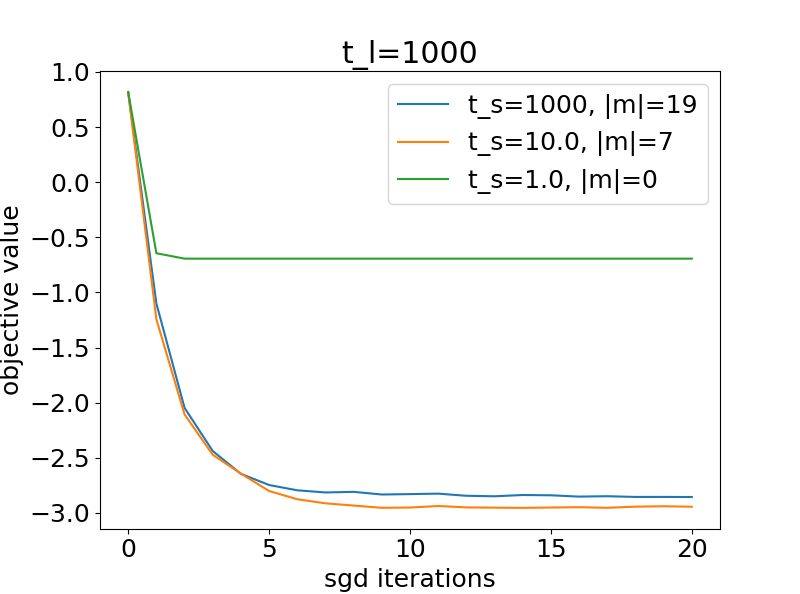
Figure 1: Convergence of the gradient descent algorithm for different choices of the relaxation constants, $t_{s}\in\{t_{l},t_{l}/100,t_{l}/1000\}$. In the legend, $|m|$ denotes the number of free parameters of the final model, ($\|m\|^{2}$ in (14)).

3.2 Transferability (CIFAR10 and CIFAR100 data, Figures 2, 3, 4, and 5)

To check the scalability transfer-learning performance of AP, we use the VGG19 Simonyan and Zisserman (2014) model ($D\sim 144\ m$ free parameters) as parent network (see Section 2.1), images and labels from CIFAR10 (10 classes, 5000+1000 images per class, referred to as ${\cal D}_{train}$ in Section 2.1) for the AP step, and images and labels from CIFAR100 (100 classes, 500+100 images per class, referred to as ${\cal D}_{new}$ in Section 2.1) to evaluate the obtained sub-architectures. The VGG sub-architectures are evaluated by fine-tuning them on new-task data sets of $5k$, $1k$ $500$, $100$, $50$ images. The new-task data sets, referred to as ${\cal D}_{new}$, are obtained by randomly sub-sampling a balanced number of images from 10 classes of CIFAR100. In particular, we compare the transfer-learning performance of VGG sub-architectures of different complexity, $|m|=D(1-{sparsity})$, ${sparsity}\in\{0.1,0.3,0.5,0.9,0.95,0.99\}$, obtained with three different methods: i) random pruning (Rnd in the plots), ii) the proposed AP approach (Ours), and iii) the Iterative Magnitude Pruning (IMP) scheme described in Frankle and Carbin (2018) (our implementation). In all cases, we report the average and standard deviations (over 5 runs) of the accuracy versus the models’ sparsity, ${sparsity}$ defined above.

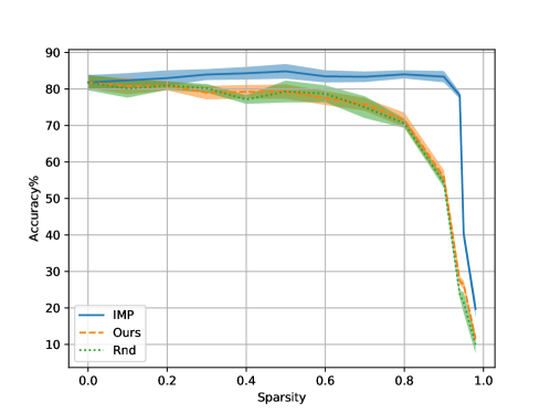
Figure 2: In-domain performance: all models are fine-tuned on $5k$ test images from CIFAR10 (same 10-class classification task used for AP).

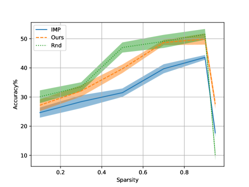
Figure 3: Transfer-learning performance for $|{\cal D}_{new}|=5k$.

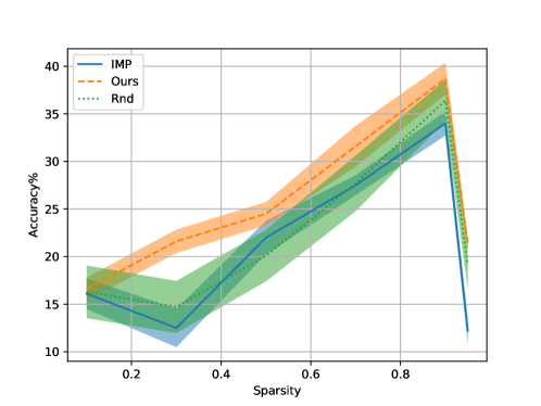
Figure 4: Transfer-learning performance for $|{\cal D}_{new}|=1k$. $|{\cal D}_{new}|=1k$.

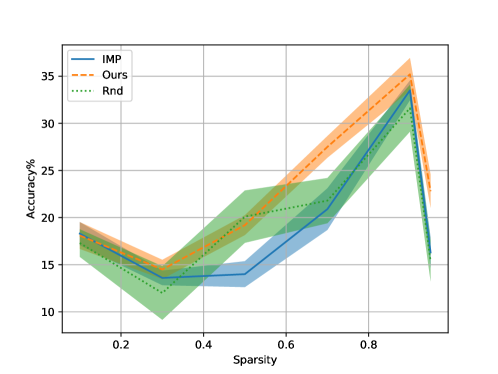
Figure 5: Transfer-learning performance for $|{\cal D}_{new}|=500$.

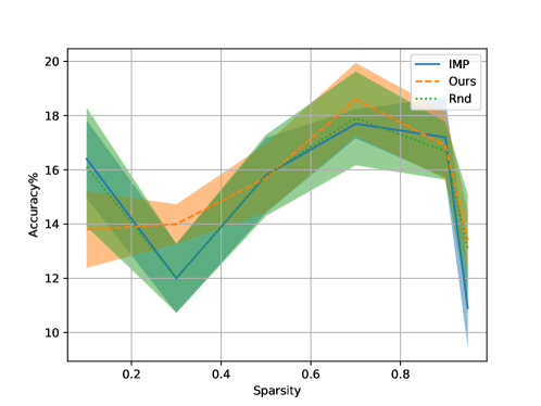
Figure 6: Transfer-learning performance for $|{\cal D}_{new}|=100$.

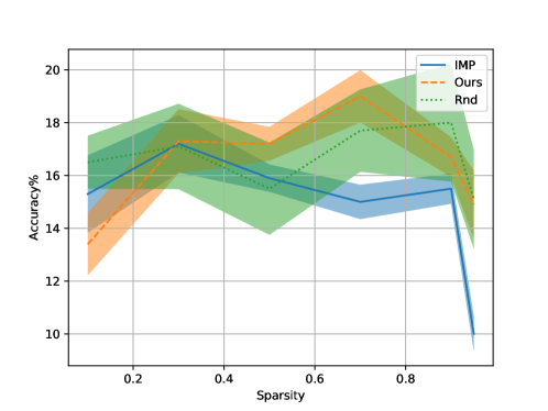
Figure 7: Transfer-learning performance for $|{\cal D}_{new}|=50$.

Sparsity	Reshuffle Ours	Reshuffle IMP
0.1	.378$\pm$.021	.300$\pm$.024
0.3	.343$\pm$.023	.332$\pm$.022
0.5	.429$\pm$.023	.342$\pm$.026
0.7	.448$\pm$.020	.376$\pm$.025
0.9	.497$\pm$.021	.100$\pm$.000
0.95	.301$\pm$.001	.100$\pm$.000
0.99	.100$\pm$.000	.100$\pm$.000

Table 1: Transfer-learning performance after random layer-wise reshuffling ($|{\cal D}_{new}|=500$).

3.3 Layer-wise sparsity (CIFAR10 and CIFAR100 data sets, Table 1)

As noticed in previous work Frankle et al. (2020), the transfer learning properties of neural architectures depends more on the layer-wise connection density than on the specific connection configuration. To test this hypothesis, we compare the transfer-learning performance of all VGG sub-architectures upon layer-wise reshuffling of the optimized binary masks. From each sub-architecture, we extract an optimal layer-wise connection density, $1-{sparsity}_{*}^{(l)}=1^{T}m_{*}^{(l)}/D^{(l)}$, $l=1,\dots,n_{layers}$, where ${sparsity}_{*}^{(l)}$ is the layer-wise sparsity and $D^{(l)}$ the total number of layer $l$ in the original VGG model, and test the transfer-learning performance of a random architecture with such an optimal layer-wise density, i.e. a random architecture with layer-wise binary masks $\tilde{m}^{(l)}$ satisfying $|\tilde{m}^{(l)}|=D^{(l)}(1-{sparsity}_{*}^{(l)})$, $l=1,\dots,n_{layers}$.

4 Discussion

4.1 Results

The proposed two-temperature approach improves both the speed and the efficiency of gradient-based algorithms in solving continuous relaxation of discrete optimization problems. Our experiment on MNIST data (see Section 3.1 and Figure 1) shows that a careful choice of the high-temperature parameter, $t_{s}$, defined in Section 2.2, may help the stability of the gradient updates. Setting the high temperature to $t_{s}\sim t_{l}/100$ makes a standard SGD algorithm reach a lower objective value in fewer iterations than for $t_{s}=t_{l}$ (equivalent to using the exact gradient in (9)) or $t_{s}=t_{l}/1000$ (higher gradient-approximation temperature). The optimized models have different complexity, as this is implicitly controlled through the regularization parameter $\lambda$ in (14). Choosing $t_{s}=t_{l}/1000$ is less efficient because the gap between the true gradient and its approximation becomes too large (in our experiments, it causes the AP optimization to prune all network connections). These results are in line with the theoretical convergence bound of Theorem 2.1.

AP can be efficiently used to extract low-complexity and transferable sub-architectures of a given large network, e.g. VGG (see Section 3.2). According to our transfer learning experiment on CIFAR10 and CIFAR100 (see Section 3.2), AP sub-architectures adapt better than random or IMP sub-architectures of the same size to solve new tasks, especially when the data available for retraining the networks on the new task is small. When $|{\cal D}_{new}|$ is big enough, random sub-architectures may also perform well, probably because their structure is not biased by training on a different domain (Figure 3). AP models are consistently better than random when fewer than 1000 data points are available (Figures 4 and 5). IMP models are worse than AP and random models in all setups, confirming that IMP produces sub-architectures that are too strongly related to the training task (Figures 3, 4, and 5). When $|{\cal D}_{new}|$ is too small, e.g. $|{\cal D}_{new}|<100$, all models perform badly, which may be due to numerical instabilities in the fine-tuning optimization phase. Interestingly, while lower-complexity models adapt better to the new domain when $|{\cal D}_{new}|$ is not too small (Figures 3, 4, and 5), this is not true when $|{\cal D}_{new}|$ contains fewer than $100$ images, i.e. 10 images per class.

The good performance of IMP models in the in-domain experiment (Figure 2) confirms their stronger link to the original task and a higher level of entanglement between the learned sub-architectures and the corresponding weights.

The results we obtained in the layer-wise reshuffling experiment (Table 1) confirm the conjecture of Frankle et al. (2020) about the importance of ink learning the right layer-wise density. A comparison between Table 1 and Figure 3 suggests that a good layer-wise density is what matters the most in making a neural architecture more transferable. Probably, the good performance of reshuffled and random-selected architectures also indicates that fine-tuning may be powerful enough to compensate for non-optimal architecture design when the number of network connections is large enough. We should note, however, that this does not happen if i) the size of the new-task data is small, suggested by the increasing performance gap between AP and random models when only 1k or 500 samples from the new task are available (Figures 4 and 5), and ii) the learned sub-architectures are too task-specific, e.g. for all IMP models.

4.2 Directions

Many more experimental setups can and should be tried. For example, it would be interesting to:

• test the performance of the method on the same data set but for different choices parent network

• see if the proposed method can handle more challenging transfer learning task, i.e. for less similar learning and testing tasks

• compare with other architecture search method (this is not easy as a fair comparison would require starting from analogous search spaces

• try other than random initialization in the fine-tuning step, as it has been proved beneficial in similar NLP transfer learning experiments (see for example Chen et al. (2020))

• study the difference between the performance of the bare architecture, i.e. with binary weights taking values in $\{-1,1\}$, which could be used as a low-memory version of the transferable models for implementation on small devices)

From the theoretical perspective, follow-up work will consist of applications of the proposed two-temperature method to other discrete optimization problems.

Appendix A Algorithms

A.1 Architecture-pruning algorithm

input: training task and data set, ${\cal D}_{train}$, parent network architecture, ${\cal A}_{parent}$, low and high inverse temperatures, e.g. $t_{l}=100$, $t_{s}=t_{l}/10$, optimization hyper-parameters, $T\in{\cal N_{+}}$ $\{\alpha_{i},\beta_{i}\}_{i=1}^{T}$,

1. let $F(\theta)=F({\cal A}_{train},\theta_{0})$, $\theta_{0}\sim{\cal N}(0,\epsilon_{\theta})^{D}$, $\epsilon_{\theta}>0$ be a randomly initialized version of the parent network.

2. let the training optimization problem be be the low-temperature approximation of (6) defined as

$$w_{*}={\rm arg}\min_{w}\left(\min_{\theta}{\cal L}(F(v_{t_{l}},\theta),{\cal D}_{train})\right)$$ (15)

$$v_{t_{l}}=\sigma(t_{l}w)$$ (16)

3. let $w_{0}\sim|{\cal N}(0,\epsilon_{w})|^{D}$, $\epsilon_{w}>0$ and solve (15) through approximate gradient updates defined by

$$w_{i+1}=w_{i}-\alpha_{i}\tilde{\nabla}_{v}{\cal L}$$

$$\tilde{\nabla}_{v}=\left.\nabla_{v}{\cal L}(z;v,\theta_{i})\right|_{v=\sigma(t_{l}w_{i})}\circ v^{\prime}\circ(1-v^{\prime})$$

$$v^{\prime}=\sigma(t_{s}w_{i})$$ (17)

$$\theta_{i+1}=\theta_{i}-\beta_{i}\left.\nabla_{\theta}{\cal L}(\sigma(t_{l}w_{i}),\theta,{\cal B}_{i})\right|_{\theta=\theta_{i}}$$ (18)

where $\{{\cal B}_{i}\subset{\cal D}_{train}\}_{i=1}^{T}$ are randomly selected batches of training examples $z=(x,y)\in{\cal d}_{train}$

output: architecture of the sub-network obtained by masking $F(\theta=1)$ with the optimized binary mask

$$m_{*}={\bf 1}[w_{T}>0]=\lim_{t_{l}\to\infty}\sigma(t_{l}w^{T})$$

A.2 Transfer learning-evaluation algorithm

input: new task and data set, ${\cal D}_{new}$, split into ${\cal D}_{retrain}$ and ${\cal D}_{test}$ unit-weight version of the parent network, $F(\theta={\bf 1})$, optimized binary mask $m_{*}\in\{0,1\}^{D}$ optimization hyper-parameters, $T\in{\mathbb{N}}_{+}$, $\{\beta_{i}\}_{i=1}^{T}$

1. let $F(\tilde{\theta}_{0})=F(m_{*}\circ\theta_{0})$, $\theta_{0}\sim{\cal N}(0,\epsilon_{\theta})^{D}$, $\epsilon_{\theta}>0$ be a randomly initialized version of the optimized sub-architecture

2. let the transfer-learning testing problem be

$$\theta*={\rm arg}\min_{\theta}{\cal L}(F(m_{*},\theta),{\cal D}_{retrain})$$

3. solve (A.2) through standard gradient descent updates

$$\theta_{i+1}=\theta_{i}-\beta_{i}m_{*}\circ\left.\nabla_{\theta}{\cal L}(m_{*},\theta,{\cal B}_{i})\right|_{\theta=\theta_{i}}$$

where $\theta_{0}\sim{\cal N}(0,\epsilon_{\theta})^{D}$, $i=1,\dots,T$, and $\{{\cal B}_{i}\subset{\cal D}_{test}\}_{i=1}^{t}$ are randomly selected batches of training examples $z=(x,y)\in{\cal D}_{test}$

output: average accuracy of $F(\tilde{\theta}*)$, $\tilde{\theta}*=m*\circ\theta*$, on ${\cal D}_{test}$

$${\rm acc}_{m_{*}}=|{\cal D}_{test}|^{-1}\sum_{(x,y)\in{\cal D}_{test}}{\bf 1}[{\rm arg}\max F(x;\tilde{\theta}*)=y]$$

A.3 Enforcing sparsity

The number of active connections in the learned architecture is determined by the number of positive entries of $w_{T}$. To encourage sparsity, we replace (17) and (18) with

$$w_{i+1}=w_{i}-\alpha_{i}\left(\tilde{\nabla}_{v}{\cal L}-2\gamma\ (\mathbf{1}+w_{i})\right)$$ (19)

$$\theta_{i+1}=\theta_{i}-\beta_{i}\left(\left.\nabla_{\theta}{\cal L}(\sigma(t_{l}w_{i}),\theta,{\cal B}_{i})\right|_{\theta=\theta_{i}}-2\gamma\ \theta_{i}\right)$$

where $\gamma$ is a regularisation parameter. This is equivalent to adding

$$\gamma\ 1^{T}\left(({\bf 1}+w)\circ({\bf 1}+w)+\theta\circ\theta\right)\approx\gamma\left(\|m\|^{2}_{0}+\|\theta\|^{2}_{2}\right)$$ (20)

in (15). The mask parameters in $w$ are initialised with small positive values and, at each iteration, the penalisation term pushes them towards $-1$, so that sparser masks can be obtained. To reach the target sparsity in a similar number of epochs we tune the hyper-parameter $\gamma$. In practice, we check the complexity of the sub-network, at each iteration and set $\alpha_{i+1}=0$ if $1^{T}{\bf 1}[w_{i}>0]<r_{sparsity}D$.

Appendix B Convergence analysis

B.1 Definitions

The results presented in this appendix are more general than the convergence bound reported in the main text. To simplify the exposition, we use a slightly different notation. In particular,

• $t_{l}$ and $t_{s}$ are called $M_{hard}$ and $M_{small}$

• $t=1,\dots,T$ is used as an upper index to label the SGD epochs (except for the learning parameters $\alpha_{t}$)

• $m_{t_{l}}=\sigma(t_{l}\theta)$ is called $v$ throughout this appendix

• $\ell(z;m_{t_{l}},p)$ and ${\cal L}_{t_{l}}(\theta)={\cal L}_{t}(\sigma(t\theta))$ of the main text are called $f(v,z)$ and $F(v)$

• Theorem 1 of the main text is Corollary B.4

• ${\cal D}_{train}$ is ${\cal D}$

• $\nabla_{v}f(v,z)$ is $\nabla f(v,z)$ defined by $[\nabla f(v,z)]_{i}=\frac{\partial}{\partial v^{\prime}_{i}}f(v^{\prime},z)|_{v^{\prime}=v}$

To avoid confusion, we list of all quantities and conventions used throughout this technical appendix:

• $d\in{\mathbf{N}}$: number of model parameters

• ${\cal Z}={\cal X}\otimes{\cal Y}$: object-label space

• $P_{Z}$: object-label distribution

• $Z\sim P_{Z}$: object-label random variable

• ${\cal D}=\{z_{n}\in{\cal Z}|z_{n}\text{ is realization of }Z\sim P_{Z}\}_{n=1}^{N}$: training data set

• $f:[0,1]^{d}\otimes{\cal Z}\to{\mathbf{R}}$: single-input classification error

• $F:[0,1]^{d}\to{\mathbf{R}}$, $F(v)=\sum_{z\in{\cal D}}f(v,z)\approx|{\cal D}|\ {E}_{Z\sim P_{Z}}(f(v,Z))$: average classification error

• $M_{soft}$ and $M_{hard}>0$, such that $0\leq M_{soft}\leq M_{hard}$: soft- and hard-binarization constants

• $\sigma(s)=\frac{1}{1+e^{-s}}\in[0,1]^{d}$ for all $s\in{\mathbf{R}}^{d}$

• $\sigma^{\prime}(s):=\sigma(s)\odot(1-\sigma(s))$, for all $s\in{\mathbf{R}}^{d}$

• $[\nabla g(s)]_{i}=\frac{\partial g(s^{\prime})}{\partial s^{\prime}_{i}}|_{s^{\prime}=s}$

• $\text{diag}(s)\in{\mathbf{R}}^{d\times d}$ is such that $[\text{diag}(s)]_{ii}=v_{i}$ and $[\text{diag}(s)]_{ij}=0$ if $i\neq j$, $i,j=1,\dots,d$

B.2 Assumptions and proofs

Assumption 2.

$f:[0,1]^{d}\otimes{\cal Z}\to{\mathbf{R}}$, is differentiable over $[0,1]^{d}$ for all $z\in{\cal Z}$ and obeys

$$\max_{v\in[0,1]^{d},z\in{\cal Z}}\|\nabla f(v,z)\|^{2}\leq G^{2},$$ (21)

$$f(v,z)-f(v^{\prime},z)\geq\nabla f(v^{\prime},z)^{T}(v-v^{\prime}),$$ (22)

for all $v,v^{\prime}\in[0,1]^{d}$ and $z\in{\cal Z}$.

Lemma B.1.

Let $f:[0,1]^{d}\otimes{\cal Z}\to{\mathbf{R}}$ be the function defined in Assumption 2 and $F:[0,1]^{d}\to{\mathbf{R}}$ be defined by

$$F(v)=\sum_{z\in{\cal D}}f(v,z)\approx|{\cal D}|\ E_{Z}(f(v,Z))$$

where ${\cal D}=\{z_{n}\in{\cal Z}|z_{n}\text{ is realization of }Z\sim P_{Z}\}_{n=1}^{N}$. Then

$$F(v)-F(v^{\prime})\geq\nabla F(v^{\prime})^{T}(v-v^{\prime}),$$ (23)

for all $v,v^{\prime}\in[0,1]^{d}$ and $z\in{\cal X}\times{\cal Y}$.

Proof of Lemma B.1

The convexity of $f$ implies the convexity of $F$ as

$$F(v)-F(v^{\prime}) =|{\cal D}|^{-1}\sum_{z\in{\cal D}}f(v,z)-f(v^{\prime},z)$$ (24)

$$\geq|{\cal D}|^{-1}\sum_{z\in{\cal D}}\nabla f(v^{\prime},z)^{T}(v-v^{\prime})$$ (25)

$$=\nabla F(v^{\prime})^{T}(v-v^{\prime}).$$ (26)

$\square$

Lemma B.2.

Let $\alpha_{t}=\frac{c}{\sqrt{t}}$, $c>0$, and $\theta^{t}\in{\mathbf{R}}^{d}$ be defined by

$$\theta^{t+1}=\theta^{t}-\alpha_{t}M_{soft}\nabla f(\sigma(M_{hard}\theta^{t}),z_{t})\odot\sigma^{\prime}(M_{soft}\theta^{t}),$$ (27)

where, for all $t=1,\dots,T$, $\sigma^{\prime}(s)=\sigma(s)\odot(1+\sigma(s))$ ($s\in{\mathbf{R}}^{d}$), and $z_{t}$ is chosen randomly in ${\cal D}$. Then, for all $t=1,\dots,T$, $v^{t}=\sigma(M_{hard}\theta^{t})$ obeys

$$v^{t+1}=v^{t}-\alpha_{t}(\nabla f(v^{t},z_{t})+r^{t}),$$ (28)

where

$$r^{t} =\nabla f(v^{t},z)-M_{hard}M_{soft}\sigma^{\prime}(M_{hard}\xi^{t})\odot\nabla f(v^{t},z)\odot\sigma^{\prime}(M_{soft}\theta^{t})$$ (29)

$$\xi^{t} \in[\theta^{t},\theta^{t}-\alpha_{t}M_{soft}\nabla f(v^{t},z)\odot\sigma^{\prime}(M_{soft}\theta^{t})]$$ (30)

for any $z_{t}\in{\cal Z}$. Furthermore, for all $t=1,\dots,T$, $r^{t}$, obeys

$$\|r^{t}\|^{2}\leq G^{2}C$$ (31)

where $G$ is defined in (2) and

$$C=M_{hard}M_{soft}\left(\frac{1}{M_{hard}M_{soft}}-2g_{max}(M_{hard})g_{max}(M_{soft})+\frac{M_{hard}M_{soft}}{16^{2}}\right)$$ (32)

$$g_{max}(M)=\sigma(M\theta_{max})(1-\sigma(M\theta_{max}))$$ (33)

$$\theta_{max}=\max_{t}|\theta^{t}|$$ (34)

Proof of Lemma B.2

Let $\sigma_{M}(s)=\sigma(Ms)$, $\sigma^{\prime}_{M}(s)=M\sigma(Ms)(1-\sigma(Ms))$, and $v=\sigma_{M}(\theta)$, for any $\theta\in{\mathbf{R}}^{d}$ and $M>0$. Then (27) is equivalent to (28) as

$$v^{t+1} =\sigma_{M_{hard}}\left(\theta^{t}-\alpha_{t}\nabla f(\sigma_{M_{hard}}(\theta^{t}),z)\odot\sigma_{M_{soft}}^{\prime}(\theta^{t})\right)$$ (35)

$$=v^{t}-\alpha_{t}\sigma_{M_{hard}}^{\prime}(\xi^{t})\odot\nabla f(\sigma_{M_{hard}}(\theta^{t}),z)\odot\sigma_{M_{soft}}^{\prime}(\theta^{t})$$ (36)

$$=v^{t}-\alpha_{t}\nabla f(v^{t},z)+\alpha_{t}r^{t}$$ (37)

$$r^{t} =\nabla f(v^{t},z)-\text{diag}\left(\sigma_{M_{hard}}^{\prime}(\xi^{t})\odot\sigma_{M_{soft}}^{\prime}(\theta^{t})\right)\cdot\nabla f(\sigma_{M_{hard}}(\theta^{t}),z)$$ (38)

$$=\nabla f(v^{t},z)-\text{diag}\left(\sigma_{M_{hard}}^{\prime}(\xi^{t})\odot\sigma_{M_{soft}}^{\prime}(\theta^{t})\right)\cdot\nabla f(v^{t},z)$$ (39)

$$\xi^{t} \in[\theta^{t},\theta^{t}-\alpha_{t}\nabla f(v^{t},z)\odot\sigma_{M_{soft}}^{\prime}(\theta^{t})]$$ (40)

where the first equality follows from $\sigma_{M}(a+b)-\sigma_{M}(a)=\sigma^{\prime}_{M}(\xi)\ b$ for some $\xi\in[a,a+b]$ (mean value theorem). For any $\theta\in{\mathbf{R}}$ and $z\in{\cal Z}$, one has

$$\|r^{t}\|^{2} =\|\nabla f(v^{t},z)\|^{2}+\|\text{diag}\left(\sigma_{M_{hard}}^{\prime}(\xi^{t})\odot\sigma_{M_{soft}}^{\prime}(\theta^{t})\right)\cdot\nabla f(v^{t},z)\|^{2}$$ (41)

$$\quad-2\nabla f(v^{t},z)^{T}\text{diag}\left(\sigma_{M_{hard}}^{\prime}(\xi^{t})\odot\sigma_{M_{soft}}^{\prime}(\theta^{t})\right)\cdot\nabla f(v^{t},z)$$ (42)

$$\leq G^{2}\left(1-2\min\sigma_{M_{hard}}^{\prime}(\xi^{t})\odot\sigma_{M_{soft}}^{\prime}(\theta^{t})+\left(\max\sigma_{M_{hard}}^{\prime}(\xi^{t})\odot\sigma_{M_{soft}}^{\prime}(\theta^{t})\right)^{2}\right)$$ (43)

$$\leq G^{2}\left(1-2\sigma_{M_{hard}}^{\prime}(\theta_{max})\sigma_{M_{soft}}^{\prime}(\theta_{max})+\left(\frac{M_{hard}M_{soft}}{16}\right)^{2}\right)$$ (44)

$$\leq G^{2}M_{hard}M_{soft}\left(\frac{1}{M_{hard}M_{soft}}-2g_{max}(M_{hard})g_{max}(M_{soft})+\frac{M_{hard}M_{soft}}{16^{2}}\right)$$ (45)

$$=G^{2}C$$ (46)

where $G$ is defined in Assumption 2, $\min a$ and $\max a$ are the smallest and largest entries of $a\in{\mathbf{R}}^{d}$, $\theta_{max}=\max_{t}|\theta^{t}|$,

$$g_{max}(M)=\sigma_{M}(\theta_{max})(1-\sigma_{M}(\theta_{max}))=\sigma(M\theta_{max})(1-\sigma(M\theta_{max})),$$

and we have used

$$\max_{s\in{\mathbf{R}}}\sigma_{M}^{\prime}(s)=\sigma_{M}^{\prime}(0)=\frac{M}{4},\quad\min_{s\in[-a,a]}=\sigma_{M}^{\prime}(s)=\sigma^{\prime}(-a)=\sigma^{\prime}(a)$$

for any $M>0$, the Cauchy-Schwarz inequality $s^{T}s^{\prime}\leq\|s\|\|s^{\prime}\|$, and $s^{T}\text{diag}(s^{\prime})\cdot s\leq(\max s^{\prime})\|s\|^{2}$, and defined

$$C=M_{hard}M_{soft}\left(\frac{1}{M_{hard}M_{soft}}-2g_{max}(M_{hard})g_{max}(M_{soft})+\frac{M_{hard}M_{soft}}{16^{2}}\right)$$

$\square$

Theorem B.3.

Let $f:[0,1]^{d}\otimes{\cal Z}\to{\mathbf{R}}$ and $F:[0,1]^{d}\to{\mathbf{R}}^{d}$ be defined as in Assumption 2 and Lemma B.1. Let $v^{t}$ and $\alpha_{t}=\frac{c}{\sqrt{t}}$ ($t=1,\dots,T$, $c>0$) be the sequence of weights defined in (28) and a sequence of decreasing learning rates and $v^{*}={\rm arg}\min_{v\in[0,1]^{d}}f(v)$. Then

$${E}\left(F(v^{T})-F(v^{*})\right)\leq\frac{1}{c\sqrt{T}}+\frac{cG^{2}(1+C)(1+\log T)}{T}$$ (47)

where the expectation is over $Z\sim P_{Z}$ and $G$ and $C$ are defined in Lemma B.2.

Proof of Theorem B.3

Assumption (2) and Lemma (B.1) imply that $F:[0,1]^{d}\to{\mathbf{R}}$ is a convex function over $[0,1]^{d}$. The first part of Lemma B.2 implies that the sequence of approximated ${\mathbf{R}}^{d}$-valued gradient updates (27) can be rewritten as the sequence of approximated $[0,1]^{d}$-valued gradient updates (28). The second part of Lemma B.2 implies that the norm of all error terms in (28) is bounded from above. In particular, as each $r^{t}$ is multiplied by the learning rate, $\alpha_{t}=\frac{c}{t}$, it is possible to show that (28) converges to a local optimum of $F:[0,1]^{d}\to{\mathbf{R}}$.

To show that (28) converges to a local optimum of $F:[0,1]^{d}\to{\mathbf{R}}$ we follows a standard technique for proving the convergence of stochastic and make the further (standard) assumption

$$E(r^{t})=0,\quad t=1,\dots,T.$$ (48)

First, we let $v^{t}$, $r^{t}$ and $\alpha_{t}$, $t=1,\dots,T$, be defined as in Lemma B.2, and $z\in{\cal D}$ be the random sample at iteration $t+1$. Then

$$\|v^{t+1}-v^{*}\|^{2} =E\left(\|v^{t+1}-v^{*}\|^{2}\right)$$ (49)

$$=\|v^{t}-v^{*}\|^{2}-2\alpha_{t}E(\nabla f(v^{t},z)-r^{t})^{T}(v^{t}-v^{*})$$ (50)

$$\quad+\alpha^{2}_{t}E\left(\|\nabla f(v^{t},\tilde{z})-r^{t}\|^{2}\right)$$

$$\leq\|v^{t}-v^{*}\|^{2}-2\alpha_{t}E(\nabla f(v^{t},z)^{T}(v^{t}-v^{*})+\alpha^{2}_{t}\left(G^{2}+E(\|r^{t}\|^{2})\right)$$ (51)

$$\leq\|v^{t}-v^{*}\|^{2}+2\alpha_{t}E(F(v^{*})-F(v^{t}))+\alpha^{2}_{t}G^{2}(1+C)$$ (52)

where $G^{2}$ and $C$ are defined in (2) and (41). Rearranging the terms one obtains

$$E(F(v^{t})-F(v^{*})) \leq\frac{\|v^{t}-v^{*}\|^{2}-\|v^{t+1}-v^{*}\|^{2}}{2\alpha_{t}}+\frac{\alpha_{t}}{2}G^{2}(1+C)$$ (53)

Since $F(v^{T})-F(v^{*})=\frac{1}{T}\sum_{t=1}^{T}\left(F(v^{t})-F(v^{*})\right)$, the bound in (53) implies

$$E\left(F(v^{T})-F(v^{*})\right) =E\left(\frac{1}{T}\sum_{t=1}^{T}\left(F(v^{t})-F(v^{*})\right)\right)$$ (54)

$$\leq\frac{1}{T}\sum_{t=1}^{T}E\left(F(v^{t})-F(v^{*})\right)$$ (55)

$$\leq\frac{1}{2cT}\sum_{t=1}^{T}\left(\sqrt{t}(\|v^{t}-v^{*}\|^{2}-\|v^{t+1}-v^{*}\|^{2})+\frac{c^{2}G^{2}(1+C)}{\sqrt{t}}\right)$$ (56)

$$=\frac{1}{2cT}\left(\sum_{t=1}^{T}(\sqrt{t+1}-\sqrt{t})\|v^{t}-v^{*}\|^{2}-T\|v^{T+1}-v^{*}\|^{2}+c^{2}G^{2}(1+C)\sum_{t=1}^{T}\frac{1}{t}\right)$$ (57)

$$\leq\frac{1}{2cT}\left(\sqrt{T}\max_{t}\{\|v^{t}-v^{*}\|^{2}\}_{t=1}^{T}+c^{2}G^{2}(1+C)(1+\log T)\right)$$ (58)

$$\leq\frac{1}{c\sqrt{T}}+\frac{cG^{2}(1+C)(1+\log T)}{T}$$ (59)

where the second line follows from the Jensen’s inequality and we have used $\sum_{t=1}^{T}(\sqrt{t+1}-\sqrt{t})\leq\sqrt{T}$ and $\sum_{t=1}^{T}\frac{1}{t}\leq 1+\log T$. $\square$

Corollary B.4.

Let $f:[0,1]^{d}\otimes{\cal Z}\to{\mathbf{R}}$ and $F:[0,1]^{d}\to{\mathbf{R}}^{d}$ be defined as in Assumption 2 and Lemma B.1. Let $\theta^{t}$ be a sequence of stochastic weight updates defined by

$$\theta^{t+1}=\theta^{t}-\alpha_{t}M_{soft}\nabla f(\sigma(M_{hard}\theta^{t}),z_{t})\odot\sigma^{\prime}(M_{soft}\theta^{t})$$

where, for all $t=1,\dots,T$, $\alpha_{t}=\frac{c}{\sqrt{t}}$ ($c>0$) and $z_{t}$ is chosen randomly in ${\cal D}$. Then

$$E(F(\sigma(M_{hard}\theta^{T}))-F(\sigma(M_{hard}\theta^{*}))\leq\frac{1}{c\sqrt{T}}+\frac{cG^{2}(1+C)(1+\log T)}{T}$$

where the expectation is over $Z\sim P_{Z}$, $\theta^{*}={\rm arg}\min_{\theta\in{\mathbf{R}}^{d}}F(\sigma(M_{hard}\theta)$, $G$ is defined in (2), and

$$C=M_{hard}M_{soft}\left(\frac{1}{M_{hard}M_{soft}}-2g_{max}(M_{hard})g_{max}(M_{soft})+\frac{M_{hard}M_{soft}}{16^{2}}\right)$$ (60)

$$g_{max}(M)=\sigma(M\theta_{max})(1-\sigma(M\theta_{max})),\quad\theta_{max}=\max_{t}|\theta^{t}|$$ (61)

Proof of Corollary B.4

The Corollary follows directly from Theorem B.3 because $\sigma$ is a strictly increasing function, which implies that the mappings ${\mathbf{R}}^{d}\to[0,1]^{d}$ and $[0,1]^{d}\to{\mathbf{R}}^{d}$ are both one-to-one. In particular, for all $t=1,\dots,T$ one has $\theta^{t}=\frac{1}{M_{hard}}\sigma^{-1}(v^{t})$ and

$$\theta^{*} :=\text{arg }\min_{\theta\in{\mathbf{R}}^{d}}F(\sigma(M_{hard}\theta))$$ (62)

$$=\frac{1}{M_{hard}}\sigma^{-1}\left(\text{arg}\min_{v\in[0,1]^{d}}F(v)|_{v=\sigma(M_{hard}\theta)}\right)$$ (63)

$$=\frac{1}{M_{hard}}\sigma^{-1}(v_{*})$$ (64)

with $v^{*}:={\rm arg}\min_{v\in[0,1]}F(v)$. It follows that $F(v^{t})\to F(v*)$ implies $F(\sigma(M_{hard}\theta^{t}))\to F(\sigma(M_{hard}\theta^{*})))$. $\square$

References

- Chen et al. (2020) Tianlong Chen, Jonathan Frankle, Shiyu Chang, Sijia Liu, Yang Zhang, Zhangyang Wang, and Michael Carbin. The lottery ticket hypothesis for pre-trained bert networks. arXiv preprint arXiv:2007.12223, 2020.
- Chen et al. (2015) Wenlin Chen, James Wilson, Stephen Tyree, Kilian Weinberger, and Yixin Chen. Compressing neural networks with the hashing trick. In International conference on machine learning, pages 2285–2294, 2015.
- Collins and Kohli (2014) Maxwell D Collins and Pushmeet Kohli. Memory bounded deep convolutional networks. arXiv preprint arXiv:1412.1442, 2014.
- Courbariaux et al. (2015) Matthieu Courbariaux, Yoshua Bengio, and Jean-Pierre David. BinaryConnect: Training deep neural networks with binary weights during propagations. In Advances in neural information processing systems, pages 3123–3131, 2015.
- Courbariaux et al. (2016) Matthieu Courbariaux, Itay Hubara, Daniel Soudry, Ran El-Yaniv, and Yoshua Bengio. Binarized neural networks: Training deep neural networks with weights and activations constrained to+ 1 or-1. arXiv preprint arXiv:1602.02830, 2016.
- et al. (2019a) Ajanthan Thalaiyasingam et al. Mirror descent view for neural network quantization. arXiv preprint:1910.08237, 2019a.
- et al. (2013) Bengio Yoshua et al. Estimating or propagating gradients through stochastic neurons for conditional computation. arXiv preprint:1308.3432, 2013.
- et al. (2016) Hou Lu et al. Loss-aware binarization of deep networks. arXiv preprint:1611.01600, 2016.
- et al. (2017) Li Hao et al. Training quantized nets: A deeper understanding. arXiv preprint:1706.02379, 2017.
- et al. (2019b) Uhlich Stefan et al. Mixed precision dnns: All you need is a good parametrization. arXiv preprint:1905.11452, 2019b.
- et al. (2019c) Xiong Huan et al. Fast large-scale discrete optimization based on principal coordinate descent. arXiv preprint:1909.07079, 2019c.
- et al. (2019d) Yin Penghang et al. Blended coarse gradient descent for full quantization of deep neural networks. Research in the Mathematical Sciences, 6(1):14, 2019d.
- et al. (2019e) Yin Penghang et al. Understanding straight-through estimator in training activation quantized neural nets. arXiv preprint:1903.05662, 2019e.
- Frankle and Carbin (2018) Jonathan Frankle and Michael Carbin. The lottery ticket hypothesis: Finding sparse, trainable neural networks. arXiv preprint arXiv:1803.03635, 2018.
- Frankle and Carbin (2019) Jonathan Frankle and Michael Carbin. The lottery ticket hypothesis: Finding sparse, trainable neural networks. arXiv: Learning, 2019.
- Frankle et al. (2020) Jonathan Frankle, Gintare Karolina Dziugaite, Daniel M Roy, and Michael Carbin. Pruning neural networks at initialization: Why are we missing the mark? arXiv preprint arXiv:2009.08576, 2020.
- Gaier and Ha (2019) Adam Gaier and David Ha. Weight agnostic neural networks. In Advances in Neural Information Processing Systems, pages 5365–5379, 2019.
- Guo (2018) Yunhui Guo. A survey on methods and theories of quantized neural networks. arXiv preprint:1808.04752, 2018.
- Han et al. (2015a) Song Han, Huizi Mao, and William J Dally. Deep compression: Compressing deep neural networks with pruning, trained quantization and huffman coding. arXiv preprint arXiv:1510.00149, 2015a.
- Han et al. (2015b) Song Han, Jeff Pool, John Tran, and William J. Dally. Learning both weights and connections for efficient neural network. ArXiv, abs/1506.02626, 2015b.
- Hu et al. (2018) Qinghao Hu, Peisong Wang, and Jian Cheng. From hashing to cnns: Training binary weight networks via hashing. In Thirty-Second AAAI Conference on Artificial Intelligence, 2018.
- Hubara et al. (2017) Itay Hubara, Matthieu Courbariaux, Daniel Soudry, Ran El-Yaniv, and Yoshua Bengio. Quantized neural networks: Training neural networks with low precision weights and activations. The Journal of Machine Learning Research, 18(1):6869–6898, 2017.
- Jacob et al. (2018) Benoit Jacob, Skirmantas Kligys, Bo Chen, Menglong Zhu, Matthew Tang, Andrew Howard, Hartwig Adam, and Dmitry Kalenichenko. Quantization and training of neural networks for efficient integer-arithmetic-only inference. In Proceedings of the IEEE Conference on Computer Vision and Pattern Recognition, pages 2704–2713, 2018.
- Liu et al. (2018) Hanxiao Liu, Karen Simonyan, and Yiming Yang. DARTS: Differentiable architecture search. arXiv preprint arXiv:1806.09055, 2018.
- Pham et al. (2018) Hieu Pham, Melody Y Guan, Barret Zoph, Quoc V Le, and Jeff Dean. Efficient neural architecture search via parameter sharing. arXiv preprint arXiv:1802.03268, 2018.
- Real et al. (2019) Esteban Real, Alok Aggarwal, Yanping Huang, and Quoc V Le. Regularized evolution for image classifier architecture search. In Proceedings of the AAAI conference on artificial intelligence, volume 33, pages 4780–4789, 2019.
- Ren et al. (2020) Pengzhen Ren, Yun Xiao, Xiaojun Chang, Po-Yao Huang, Zhihui Li, Xiaojiang Chen, and Xin Wang. A comprehensive survey of neural architecture search: Challenges and solutions. arXiv preprint arXiv:2006.02903, 2020.
- Shen et al. (2019) Mingzhu Shen, Kai Han, Chunjing Xu, and Yunhe Wang. Searching for accurate binary neural architectures. In Proceedings of the IEEE International Conference on Computer Vision Workshops, pages 0–0, 2019.
- Simonyan and Zisserman (2014) Karen Simonyan and Andrew Zisserman. Very deep convolutional networks for large-scale image recognition. arXiv preprint arXiv:1409.1556, 2014.
- Soudry et al. (2014) Daniel Soudry, Itay Hubara, and Ron Meir. Expectation backpropagation: Parameter-free training of multilayer neural networks with continuous or discrete weights. In Advances in Neural Information Processing Systems, pages 963–971, 2014.
- Stanley and Miikkulainen (2002) Kenneth O Stanley and Risto Miikkulainen. Evolving neural networks through augmenting topologies. Evolutionary computation, 10(2):99–127, 2002.
- Xie et al. (2019) Sirui Xie, Hehui Zheng, Chunxiao Liu, and Liang Lin. Snas: stochastic neural architecture search. In International Conference on Learning Representations, 2019.
- You et al. (2020) Shan You, Tao Huang, Mingmin Yang, Fei Wang, Chen Qian, and Changshui Zhang. Greedynas: Towards fast one-shot nas with greedy supernet. arXiv preprint arXiv:2003.11236, 2020.
- Yu et al. (2019) Haonan Yu, Sergey Edunov, Yuandong Tian, and Ari S Morcos. Playing the lottery with rewards and multiple languages: lottery tickets in rl and nlp. arXiv preprint arXiv:1906.02768, 2019.
- Zhou et al. (2016) Shuchang Zhou, Yuxin Wu, Zekun Ni, Xinyu Zhou, He Wen, and Yuheng Zou. Dorefa-net: Training low bitwidth convolutional neural networks with low bitwidth gradients. arXiv preprint arXiv:1606.06160, 2016.
- Zoph and Le (2016) Barret Zoph and Quoc V Le. Neural architecture search with reinforcement learning. arXiv preprint arXiv:1611.01578, 2016.