Estimation and Inference in Factor Copula Models with Exogenous Covariates

Abstract

A factor copula model is proposed in which factors are either simulable or estimable from exogenous information. Point estimation and inference are based on a simulated methods of moments (SMM) approach with non-overlapping simulation draws. Consistency and limiting normality of the estimator is established and the validity of bootstrap standard errors is shown. Doing so, previous results from the literature are verified under low-level conditions imposed on the individual components of the factor structure. Monte Carlo evidence confirms the accuracy of the asymptotic theory in finite samples and an empirical application illustrates the usefulness of the model to explain the cross-sectional dependence between stock returns.

Keywords: factor analysis, simulation estimator, empirical process, dependence modeling.
JEL classifications: C13, C15, C22.

1 Introduction

Factor copula models have been successfully introduced as a means to cope with data of high cross-sectional dimensionality; see, e.g., Krupskii and Joe (2013), Creal and Tsay (2015), and Oh and Patton (2017). The use of a latent factor structure offers an economically intuitive yet flexible way to multivariate modeling that parsimoniously handles commonly encountered characteristics of financial time series like, for example, the tail asymmetry and tail dependence described by Hansen (1994). Recently, some research effort has been devoted to incorporate time variation and exogenous information to factor copula models; see, e.g., Creal and Tsay (2015), Oh and Patton (2018), Opschoor et al. (2020), and Krupskii and Joe (2020). For example, Oh and Patton (2018) and Opschoor et al. (2020), by utilizing the generalized autoregressive score (GAS) framework of Creal et al. (2013), consider specifications with latent factors and time-varying loadings that may depend on exogenous information. We contribute to this literature by introducing a class of factor copula models with exogenous, (partly) observable factors, an idea reminiscent of Bernanke et al. (2005), Boivin et al. (2009), and Stock and Watson (2005). Contrary to the above cited factor copula models, we take a step back and treat the, possibly group-specific, loadings as time-invariant constants and the SMM estimator employed here is build on the unconditional copula—a concession in the name of tractability that frees us from the necessity of specifying parametric marginals [e.g., Oh and Patton (2018)] or a closed form likelihood of the copula [e.g., Opschoor et al. (2020)] and thereby allows for a large variety of ‘covariate-augmented’ factor copulas, nesting the model Oh and Patton (2017) as a special case.

Since the copula likelihood is rarely available in closed form for the model class considered here, an SMM framework for estimation and inference is proposed which uses the general principles outlined by Oh and Patton (2013). Our main contribution is a novel distinction between simulable factors and factors that are estimable from exogenous information. Following the seminal SMM literature of McFadden (1989), Pakes and Pollard (1989), and Lee (1992), we exploit the benefits from non-overlapping simulation draws. The incorporation of exogenous covariates considerably complicates the development of an asymptotic theory as many arguments made by Oh and Patton (2013) do not apply. Nevertheless, we show that all technical hurdles can be overcome by combining recent developments from copula empirical process theory [see, e.g., Bücher and Volgushev (2013), Berghaus et al. (2017), and Neumeyer et al. (2019)] with a seminal result for extremum estimation with nonsmooth objective function due to Newey and McFadden (1994). In consequence, consistency, limiting normality, and validity of bootstrap standard errors are established. In doing so, we derive the stochastic equicontinuity of the objective function from primitive conditions on the distributional characteristics of the factor structure using the functional central limit theorem (FCLT) of Andrews and Pollard (1994) for $\alpha$-mixing triangular arrays. The theory developed here verifies earlier equicontinuity results from the literature that made use of high-level conditions; see, e.g., Oh and Patton (2013), Manner et al. (2019), and Manner et al. (2021). Since stochastic equicontinuity is an essential ingredient of the asymptotic theory that links pointwise and uniform properties, more primitive conditions are of utmost interest. An application to dependence modeling of a cross-section of stock returns of eleven financial companies illustrates the theoretical results and highlights how the incorporation of estimable factors can help to achieve improvements in model performance.

The remainder of this paper is organized as follows. Section 2 introduces the model. The main results for SMM estimation and inference are contained in Section 3. A small Monte Carlo exercise is conducted in Section 4 and an empirical application can be found in Section 5. Section 6 briefly summarizes and concludes the paper.

2 Model

Our aim is to capture the dependence structure among the cross-sectional entities of the $n\times 1$ vector of financial assets $Y_{t}\coloneqq(Y_{1,t},\dots,Y_{n,t})^{\prime}$ in time-period $t\in\{1,\dots,T\}$, conditional on the available information $\mathcal{F}_{t}\coloneqq\sigma(\{Y_{j}^{\raisebox{1.0pt}{{\footnotesize$*$}}},Y_{j-1}:j\leq t\})$, where $Y_{t}^{\raisebox{1.0pt}{{\footnotesize$*$}}}$ represents a vector of exogenous regressors. The number of financial assets $n$ might be large but is assumed finite. If the marginal conditional distributions $Y_{i,t}\mid\mathcal{F}_{t}\sim\textsf{H}_{i,t}$ are continuous, we can follow Patton (2006) and uniquely decompose the joint conditional distribution $Y_{t}\mid\mathcal{F}_{t}\sim\textsf{H}_{t}$ into its $n$ margins and a copula function $\textsf{C}_{t}:[0,1]^{n}\mapsto[0,1]$, where $\textsf{C}_{t}(\cdot)$ completely describes the dependence conditionally on $\mathcal{F}_{t}$; i.e., $\textsf{H}_{t}(x_{1},\dots,x_{n})=\textsf{C}_{t}\{\textsf{H}_{1,t}(x_{1}),\dots,\textsf{H}_{n,t}(x_{n})\}$, $x_{i}\in\mathbb{R},$ $i\in\{1,\dots,n\}$. Following, among others, Chen and Fan (2006), Oh and Patton (2013), and Fan and Patton (2014, Section 2.1), we assume for the $n$ assets parametric location-scale specifications of the form

$$Y_{i,t}=\mu_{1,i}(\mathcal{F}_{t},\lambda_{0})+\mu_{2,i}(\mathcal{F}_{t},\lambda_{0})\eta_{i,t},$$ (2.1)

where, for each $i\in\{1,\dots,n\}$, $\{\eta_{i,t}:t\geq 1\}$ are i.i.d. innovations independent of $\mathcal{F}_{t}$, while $\mu_{1,i}$ and $\mu_{2,i}$ are $\mathcal{F}_{t}$-measurable parametric specifications of the conditional mean $\mu_{1,i}(\mathcal{F}_{t},\lambda)=\textsf{E}[Y_{i,t}\mid\mathcal{F}_{t}]$ and the conditional standard deviation $\mu_{2,i}(\mathcal{F}_{t},\lambda)=\sqrt{\textsf{var}[Y_{i,t}\mid\mathcal{F}_{t}]}$ that are known up to the true $r\times 1$ parameter vector $\lambda=\lambda_{0}\in\Lambda_{0}\subset\mathbb{R}^{r}$. In particular, we assume that

$$\mu_{j,i}(\mathcal{F}_{t},\lambda)=\mu_{j,i}(R_{t}(\lambda),\lambda),\;\;j\in\{1,2\},\,i\in\{1,\dots,n\},$$ (2.2)

where, for any $\lambda\in\Lambda$, the $p_{\textsf{R}}\times 1$ random vector $R_{t}(\lambda)$ is $\mathcal{F}_{t}$-measurable with components that may parametrically depend on the entire history $\mathcal{F}_{t}$ through $\lambda$. For example, this model class includes nonlinear autoregressions (AR) with nonlinear autoregressive conditional heteroskedasticity (ARCH), in which case the dependence of $R_{t}(\lambda)$ on $\lambda$ is superfluous, as well as nonlinear generalized autoregressive conditional heteroskedasticity (GARCH) as illustrated below for the GJR model of Glosten et al. (1993).

Example: Consider the AR(1) model $Y_{i,t}=\gamma_{i}Y_{i,t-1}+\mu_{2,i,t}\eta_{i,t}$, with conditional heteroskedasticity $\mu_{2,i,t}^{2}=\omega_{i}+(\beta_{i}+\eta_{i}1\{\varepsilon_{i,t-1}(\gamma_{i})<0\})\varepsilon_{i,t-1}^{2}(\gamma_{i})+\alpha_{i}\mu_{2,i,t-1}^{2}$ for $\varepsilon_{i,t}(\gamma_{i})\coloneqq Y_{i,t}-\gamma_{i}Y_{i,t-1}$. In accordance with our notation, let $\lambda=(\gamma_{1},\dots,\gamma_{n},\alpha_{1},\dots,\alpha_{n},\omega_{1},\dots,\omega_{n},\beta_{1},\dots,\beta_{n},\eta_{1},\dots,\eta_{n})^{\prime}$ be the $r\times 1$ parameter vector collecting all unknowns for $r=5n$. Following the discussion in Yang (2006), by suitably restricting $\Lambda_{0}\subset\mathbb{R}^{r}$, this specification can be cast in form of (2.1) and (2.2) if we set $\mu_{1,i}(\mathcal{F}_{t},\lambda)=\gamma_{i}Y_{i,t-1}$, $R_{t}(\lambda)=(Y_{t-1}^{\prime},\tilde{R}_{t}(\lambda)^{\prime})^{\prime}$, where $\tilde{R}_{t}(\lambda)=(\tilde{R}_{1,t}(\lambda),\dots,\tilde{R}_{n,t}(\lambda))^{\prime}$, with $\tilde{R}_{i,t}(\lambda)=\sum_{j\,=\,1}^{\infty}\alpha_{i}^{j-1}g_{i}\{Y_{i,t-j}-\gamma_{i}Y_{i,t-1},\eta_{i}\}$, $g(x,a)=x^{2}+a1\{x<0\}x^{2}$, and $\mu_{2,i}(R_{t}(\lambda),\lambda)=\beta_{i}\tilde{R}_{i,t}(\lambda)+\omega_{i}/(1-\alpha_{i})$.

Since we assume that individually $\eta_{i,t}$ are independent of $\mathcal{F}_{t}$ and, by Eq. (2.1), $\eta_{i,t}=\{Y_{i,t}-\mu_{1,i}(\mathcal{F}_{t},\lambda_{0})\}/\mu_{2,i}(\mathcal{F}_{t},\lambda_{0})$, we can –assuming continuous margins $\textsf{F}_{i}(\eta_{i,t}\leq x_{i})\coloneqq\textsf{P}(\eta_{i,t}\leq x_{i})$, $i\in\{1,\dots,n\}$– rephrase the conditional joint distribution of $Y_{t}$ in terms of the innovation ranks $V_{i,t}\coloneqq\textsf{F}_{i}(\eta_{i,t})$ as

$$\begin{split}\textsf{H}_{t}(x_{1},\dots,x_{n})=\,&\textsf{C}_{t}\{\textsf{F}_{1}(x_{1}),\dots,\textsf{F}_{n}(x_{n})\},\\ \textsf{C}_{t}(u_{1},\dots,u_{n})=\,&\textsf{P}(V_{1,t}\leq u_{1},\dots,V_{n,t}\leq u_{n}\mid\mathcal{F}_{t}),\end{split}$$ (2.3)

$u_{i}\in[0,1]$, $i\in\{1,\dots,n\}$. While the effect of $\mathcal{F}_{t}$ on the margins has been completely removed by the use of the location-scale model (2.1), the joint cross-sectional distribution of $\eta_{t}\coloneqq(\eta_{1,t},\dots,\eta_{n,t})^{\prime}$ is allowed to depend on $\mathcal{F}_{t}$ through some ‘exogenous’ vector $Z_{t}$. That is, we assume that

$$\textsf{C}_{t}(u_{1},\dots,u_{n})=\textsf{P}(V_{1,t}\leq u_{1},\dots,V_{n,t}\leq u_{n}\mid\mathcal{F}_{t})=\textsf{P}(V_{1,t}\leq u_{1},\dots,V_{n,t}\leq u_{n}\mid Z_{t}).$$ (2.4)

We do not model the conditional copula directly but we assume that the unconditional copula

$$\textsf{C}(u_{1},\dots,u_{n})=\textsf{P}(V_{1,t}\leq u_{1},\dots,V_{n,t}\leq u_{n}),$$ (2.5)

can be generated from an auxiliary factor model via

$$\textsf{G}(x_{1},\dots,x_{n})=\textsf{C}\{G_{1}(x_{1}),\dots,G_{n}(x_{n})\},\;x_{i}\in\mathbb{R},$$ (2.6)

where $G_{i}(x_{i})\coloneqq\textsf{P}(X_{i,t}\leq x_{i})$ represents the $i$-th margin of

$$X_{i,t}=a_{0,i}^{\prime}F_{t}+b_{0,i}^{\prime}Z_{t}+\varepsilon_{i,t}$$ (2.7)

and $\textsf{G}(x)\coloneqq\textsf{P}(X_{1,t}\leq x_{1},\dots,X_{n,t}\leq x_{n})$, $x\coloneqq(x_{1},\dots,x_{n})^{\prime}\in\mathbb{R}^{n}$, is the corresponding joint distribution. As defined below, $F_{t}$ and $\varepsilon_{i,t}$ denote latent factors and the idiosyncratic component, respectively. It is crucial to stress that the margins $G_{i}$, $i\in\{1,\dots,n\}$, can differ from the univariate distributions of the observed data and are not of interest here. Rather, Eq. (2.7) serves as a means to generate the copula C that determines the joint distribution. Since any effect of $\mathcal{F}_{t}$ on the margins has been filtered out while the conditional distribution is only affected by $\mathcal{F}_{t}$ through the regressor, the unconditional copula obtains directly by taking the expectation with respect to $Z_{t}$, i.e. $\textsf{C}(\cdot)=\textsf{E}[\textsf{C}_{t}(\cdot)]$.

Oh and Patton (2018) or Opschoor et al. (2020) consider a related specification. Contrary to our approach, however, they model the conditional copula directly, i.e. they consider a conditional copula $\textsf{C}_{t}=\textsf{C}(\theta_{0,t})$ indexed by a time-varying copula parameter $\theta_{0,t}\coloneqq\theta_{0}(Z_{t})$ that is driven by GAS-dynamics so that $Z_{t}=(\eta_{1}^{\prime},\dots,\eta_{t-1}^{\prime})^{\prime}$. We, on the other hand, assume that all components of the factor model including $Z_{t}$ are $i.i.d.$. To make these notions precise, Assumption A formalizes the characteristics of the factor model. It constitutes a naturally extension of Oh and Patton (2017).

Assumption A

.

1. $\{Z_{t}:t\geq 1\}$, $\{F_{t}:t\geq 1\}$ and $\{\varepsilon_{t}:t\geq 1\}$ are mutually independent $i.i.d.$ sequences with $\varepsilon_{i,t}\perp\varepsilon_{j,t}$, $i,j\in\{1,\dots,n\}$ and $F_{t,i}\perp F_{t,j}$, $i,j\in\{1,\dots,p_{\alpha}\}$;

2. $\{X_{t},\eta_{t}:t\geq 1\}$ is an i.i.d. sequence.

The peculiar feature of Eq. (2.7), and the main contribution of this paper, is the distinction between simulable and observable factors: while $F_{t}\coloneqq(F_{t,1},\dots,F_{t,p_{\alpha}})^{\prime}$ is a $p_{\alpha}\times 1$ vector of latent random variables with known parametric distribution, the $p_{\beta}\times 1$ vector $Z_{t}\coloneqq(Z_{t,1},\dots,Z_{t,p_{\beta}})^{\prime}$ can be recovered from observed data based on econometric tools. Therefore, $Z_{t}$ is also referred to as the estimable factor. More specifically, both $F_{t}$ and $\varepsilon_{i,t}$ are i.i.d. with parametric distributions

$$\textsf{D}_{\varepsilon}(x;\,\delta_{0})\coloneqq\textsf{P}(\varepsilon_{i,t}\leq x),\;\;\;\textsf{D}_{F,j}(x;\,\gamma_{0,j})\coloneqq\textsf{P}(F_{t,j}\leq x),\,j\in\{1,\dots,p_{\alpha}\},$$

which are partially known up to the $p_{\delta}\times 1$ vector $\delta_{0}\coloneqq(\delta_{0,1},\dots,\delta_{0,p_{\delta}})^{\prime}$ and the $p_{\alpha}p_{\gamma}\times 1$ vector $\gamma_{0}\coloneqq(\gamma_{0,1}^{\prime},\dots,\gamma_{0,p_{\alpha}}^{\prime})^{\prime}$, with $\gamma_{0,j}\coloneqq(\gamma_{0,j,1},\dots,\gamma_{0,j,{p_{\gamma}}})^{\prime}$, respectively. On the other hand, the distribution of the vector $Z_{t}$ is unknown but we assume that its components $Z_{t,j}$ can be represented as i.i.d. innovations of an observable $\mathcal{F}_{t}$-measurable processes $W_{t,j}$ given by

$$Z_{t,j}=W_{t,j}-\sigma_{j}(\mathcal{W}_{t},\nu_{0}),\;\;j\in\{1,\dots,p_{\beta}\},$$ (2.8)

where the measurable functions $\sigma_{j}(\cdot,\nu)$ are known up to the $m\times 1$ vector $\nu=\nu_{0}\in\mathcal{V}_{0}\subset\mathbb{R}^{m}$; the i.i.d. innovations $Z_{t,j}$ are independent of the history $\mathcal{W}_{t}\subset\mathcal{F}_{t-1}$. Similar to the specification of Eq. (2.2), we assume that $\sigma_{j}(\mathcal{W}_{t},\nu)=\sigma_{j}(M_{t}(\nu),\nu)$, where the $p_{\textsf{M}}\times 1$ vector $M_{t}(\nu)$ comprises short-range dependent covariates, possibly including lagged dependent variables, whose components may be parametrically generated from the complete history $\mathcal{W}_{t}$. We cannot allow for both time-varying conditional means and variances to ensure that the limiting distribution of the SMM estimator is unaffected by the first step estimation of $\nu_{0}$. Note, however, that several models with time-varying conditional variance that obey $\tilde{W}_{t}=\tilde{\sigma}(M_{t}(\nu),\nu)\tilde{Z}_{t}$, $\operatorname*{\textsf{sup}}_{x,y}\tilde{\sigma}(x,y)>0$, can be cast in form of (2.8) by setting $W_{t}\coloneqq\textsf{log}|\tilde{W}_{t}|$, $\sigma_{t}(M_{t}(\nu),\nu)\coloneqq\textsf{log}\,\tilde{\sigma}_{t}(M_{t}(\nu),\nu)$, and $Z_{t}\coloneqq\textsf{log}|\tilde{Z}_{t}|$.

As in Oh and Patton (2017, Section 4.2) and Opschoor et al. (2020, Section 2.1.1), it is assumed that the factor loadings $a_{0,i}\coloneqq(a_{0,i,1},\dots,a_{0,i,p_{\alpha}})^{\prime}$ and $b_{0,i}\coloneqq(b_{0,i,1},\dots,b_{0,i,p_{\beta}})^{\prime}$ can be grouped into a small number of $Q$ group-specific coefficients $\alpha_{0,q}\coloneqq(\alpha_{0,q,1},\dots,\alpha_{0,q,p_{\alpha}})^{\prime}$ and $\beta_{0,q}\coloneqq(\beta_{0,q,1},\dots,\beta_{0,q,p_{\beta}})^{\prime}$, $q\in\{1,\dots,Q\}$. Put differently, there exists a finite collection of disjoint sets $\{\mathcal{G}_{1},\dots,\mathcal{G}_{Q}\}$ partitioning the cross-sectional index set $\{1,\dots,n\}$ such that $a_{0,i}=a_{0,j}=\alpha_{0,q}$ and $b_{0,i}=b_{0,j}=\beta_{0,q}$ for any $i,j\in\mathcal{G}_{q}$, $q\in\{1,\dots,Q\}$. Importantly, this ‘block-equidependent’ factor structure implies that the number of latent marginals needed to be specified reduces from $n$ to $Q$ distinct distributions $\textsf{G}_{1},\dots,\textsf{G}_{Q}$, say, so that $G_{i}(x)=G_{j}(x)\eqqcolon\textsf{G}_{q}(x)$ for any $i,j\in\mathcal{G}_{q}$, $q\in\{1,\dots,Q\}$. Throughout, the group assignment is assumed to be known.

3 SMM-based Estimation

The object of interest is the $p\times 1$ vector $\theta_{0}\coloneqq(\alpha_{0,1}^{\prime},\beta_{0,1}^{\prime},\dots,\alpha_{0,Q}^{\prime},\beta_{0,Q}^{\prime},\gamma_{0}^{\prime},\delta_{0}^{\prime})^{\prime}\in\Theta\subseteq\mathbb{R}^{p}$, which, in view of the latent factor structure (2.6), collects all $p\coloneqq Q(p_{\alpha}+p_{\beta})+p_{\alpha}p_{\gamma}+p_{\delta}$ unknown copula parameters. A different parameter vector $\theta\coloneqq(\alpha_{1}^{\prime},\beta_{1}^{\prime},\dots,\alpha_{Q}^{\prime},\beta_{Q}^{\prime},\gamma^{\prime},\delta^{\prime})^{\prime}\in\Theta$ gives rise to an alternative factor structure

$$X_{i,t}(d_{i})\coloneqq a_{i}^{\prime}F_{t}(\gamma)+b_{i}^{\prime}Z_{t}+\varepsilon_{i,t}(\delta),$$ (3.9)

say, where the notational conventions $X_{i,t}(d_{i})$, $F_{t}(\gamma)\coloneqq(F_{t,1}(\gamma_{1}),\dots,F_{t,p_{\alpha}}(\gamma_{p_{\alpha}}))^{\prime}$, and $\varepsilon_{i,t}(\delta)$ are used to make the dependence of the various quantities on the $(p_{\alpha}+p_{\beta}+p_{\alpha}p_{\gamma}+p_{\delta})\times 1$ vector $d_{i}\coloneqq(a_{i}^{\prime},b_{i}^{\prime},\gamma^{\prime},\delta^{\prime})^{\prime}$ explicit; e.g., $\varepsilon_{i,t}(\delta)\sim\textsf{D}_{\varepsilon}(\delta)$ and $F_{t,j}(\gamma_{j})\sim\textsf{D}_{F,j}(\gamma_{j})$, $j\in\{1,\dots,p_{\alpha}\}$. The block-equidependent design ensures that

$$d_{i}=d_{j}=\theta_{q},\quad\forall\,i,j\in\mathcal{G}_{q},\;q\in\{1,\dots,Q\},$$ (3.10)

where the $(p_{\alpha}+p_{\beta}+p_{\alpha}p_{\gamma}+p_{\delta})\times 1$ vector $\theta_{q}\coloneqq(\alpha_{q}^{\prime},\beta_{q}^{\prime},\delta^{\prime},\gamma^{\prime})^{\prime}$ contains the parameters specific to the $q$-th group. Thus, with a slight abuse of notation, ${\displaystyle\theta=\cup_{q\,=\,1}^{Q}\theta_{q}}$. For each $\theta\in\Theta$, Eq. (3.9) generates a differently parametrized copula

$$\begin{split}\textsf{C}(u_{1},\dots,u_{n};\theta)\coloneqq\,&\textsf{P}\{U_{1,t}(d_{1})\leq u_{1},\dots,U_{n,t}(d_{n})\leq u_{n}\},\\ U_{i,t}(d_{i})\coloneqq\,&G_{i}(X_{i,t}(d_{i});d_{i}),\\ G_{i}(x_{i};d_{i})\coloneqq\,&\textsf{P}\{X_{i,t}(d_{i})\leq x_{i}\},\,u_{i}\in[0,1],\,x_{i}\in\mathbb{R}.\end{split}$$ (3.11)

Importantly, due to the block-equidependent design and Eq. (3.10), we have for any two cross-sectional indices belonging to the same group

$$G_{i}(x;d_{i})=G_{j}(x;d_{j})\eqqcolon\textsf{G}_{q}(x;\theta_{q}),\quad i,j\in\mathcal{G}_{q},\,q\in\{1,\dots,Q\},$$

say, so that $G_{i}(X_{i,t}(d_{i});d_{i})=U_{i,t}(d_{i})=U_{i,t}(\theta_{q})=\textsf{G}_{q}(X_{i,t}(\theta_{q});\theta_{q})$.

The simulation-based estimation uses Assumption B below to estimate the true value of $\theta\in\Theta$ given by $\theta_{0}=\cup_{q\,=\,1}^{Q}\theta_{0,q}$, $\theta_{0,q}=(\alpha_{0,q}^{\prime},\beta_{0,q}^{\prime},\gamma_{0}^{\prime},\delta_{0}^{\prime})^{\prime}$.

Assumption B

.

1. $\textsf{C}(u_{1},\dots,u_{n})=\textsf{C}(u_{1},\dots,u_{n};\theta)$ uniformly in $(u_{1},\dots,u_{n})^{\prime}\in[0,1]^{n}$ if and only if $\theta=\theta_{0}$, where $\theta_{0}\in\Theta\subset\mathbb{R}^{p}$. The parameter space $\Theta$ is compact.

2. 1. The joint distribution $\textsf{F}(x_{1},\dots,x_{n})=\textsf{P}(\eta_{1,t}\leq x_{1},\dots,\eta_{n,t}\leq x_{n})$ is continuous with continuous marginal distributions $\textsf{F}_{i}(x_{i})$, $x_{i}\in\mathbb{R}$, $i\in\{1,\dots,n\}$.

   2. The joint distribution $\textsf{G}(x_{1},\dots,x_{n};\theta)=\textsf{P}(X_{1,t}(d_{1})\leq x_{1},\dots,X_{n,t}(d_{n})\leq x_{n})$ is continuous with continuous marginal distributions $G_{i}(x_{i};d_{i})$, $x_{i}\in\mathbb{R}$, $i\in\{1,\dots,n\}$, uniformly in $\theta\in\Theta$.

Assumption B formalizes the introductory notion of a factor copula; i.e., the unknown copula $\textsf{C}(u_{1},\dots,u_{n})$ can be generated by the latent factor structure for a suitable choice of $\theta=\theta_{0}\in\Theta$.

3.1 Independent Simulations

Akin to the ‘independent simulation’ scheme known from classical SMM estimation [see, e.g. McFadden (1989), Pakes and Pollard (1989), and Lee (1992)], we generate for a given candidate value $\theta\in\Theta\subset\mathbb{R}^{p}$ a random sample $\{(F_{t,s}(\gamma)^{\prime},\varepsilon_{i,t,s}(\delta))^{\prime}:i=1,\dots,n,\,t=1,\dots,T,\,s=1,\dots,S\}$ to obtain a version of the auxiliary factor model

$$X_{i,t,s}(d_{i})\coloneqq a_{i}^{\prime}F_{t,s}(\gamma)+b_{i}^{\prime}Z_{t}+\varepsilon_{i,t,s}(\delta),$$ (3.12)

where $F_{t,s}(\gamma)\coloneqq(F_{t,s,1}(\gamma_{1}),\dots,F_{t,s,p_{\alpha}}(\gamma_{p_{\alpha}}))^{\prime}$. Hence, we sample for each time period $t$ a new batch of $S$ random variables from $\textsf{D}_{\varepsilon}$ and $\textsf{D}_{F,j}$, $j\in\{1,\dots,p_{\alpha}\}$. More specifically, let $\textsf{D}_{\varepsilon}^{-1}$ and $\textsf{D}_{F,j}^{-1}$ denote the inverse distribution functions of $\varepsilon_{t}$ and $F_{t,j}$, $j\in\{1,\dots,p_{\alpha}\}$, respectively. We may then write $\varepsilon_{i,t,s}(\delta)\coloneqq\textsf{D}_{\varepsilon}^{-1}(\varepsilon_{i,t,s}^{\raisebox{0.1pt}{{\footnotesize$*$}}};\delta)$ and $F_{t,s}(\gamma)\coloneqq\textsf{D}_{F}^{-1}(F_{t,s}^{\raisebox{1.0pt}{{\footnotesize$*$}}};\gamma)$, with $\textsf{D}_{F}^{-1}(F_{t,s}^{\raisebox{1.0pt}{{\footnotesize$*$}}};\gamma)\coloneqq(\textsf{D}_{F,1}^{-1}(F_{t,s,1}^{\raisebox{1.0pt}{{\footnotesize$*$}}};\gamma_{1}),\dots,\textsf{D}_{F,p_{\alpha}}^{-1}(F_{t,s,p_{\alpha}}^{\raisebox{1.0pt}{{\footnotesize$*$}}};\gamma_{p_{\alpha}}))^{\prime}$, where $F_{t,s}^{\raisebox{1.0pt}{{\footnotesize$*$}}}\coloneqq(F_{t,s,1}^{\raisebox{1.0pt}{{\footnotesize$*$}}},\dots,F_{t,s,p_{\alpha}}^{\raisebox{1.0pt}{{\footnotesize$*$}}})^{\prime}$ and $\varepsilon_{i,t,s}^{\raisebox{0.1pt}{{\footnotesize$*$}}}$ denote independent draws of i.i.d. standard uniform random variates which are drawn once. Note that for our estimation procedure we hold the underlying random draws $F_{t,s}^{\raisebox{1.0pt}{{\footnotesize$*$}}}$ and $\varepsilon_{i,t,s}^{\raisebox{0.1pt}{{\footnotesize$*$}}}$ fixed while $\theta$ is allowed to vary over the compact set $\Theta$. This is important to ensure uniform convergence of simulated moments and to facilitate convergence of the numerical optimization routine used to find $\theta_{0}$; see Gouriéroux and Monfort (1997, p. 29) and Pakes and Pollard (1989, p. 1048) for further remarks. Since $Z_{t}$ might be unobservable, we will replace the unknown innovation with $\hat{Z}_{t}(\hat{\nu}_{T})\coloneqq(\hat{Z}_{t,1}(\hat{\nu}_{T}),\dots,\hat{Z}_{t,p_{\beta}}(\hat{\nu}_{T}))^{\prime}$, where $\hat{Z}_{t,j}(\nu)\coloneqq W_{t,j}-\sigma_{j}(M_{t}(\nu),\nu)$, $j\in\{1,\dots,p_{\beta}\}$, represents the generalized residual. The estimator $\hat{\nu}_{T}$ is assumed to be $\sqrt{T}$-consistent for the $m\times 1$ vector $\nu_{0}$ satisfying certain mild regularity conditions outlined below; for example, in the empirical application maximum likelihood estimation is used. Therefore, a feasible counterpart of Eq. (3.12) is obtained from

$$\hat{X}_{i,t,s}(d_{i},\hat{\nu}_{T})\coloneqq a_{i}^{\prime}F_{t,s}(\gamma)+b_{i}^{\prime}\hat{Z}_{t}(\hat{\nu}_{T})+\varepsilon_{i,t,s}(\delta).$$ (3.13)

3.2 The Estimator

Throughout, the cross-sectional dimension $n$ might be large but is considered fixed, while asymptotics are carried out as $T\rightarrow\infty$; the number of simulation draws $S$ can either be fixed or a function of $T$ such that $S\coloneqq S(T)\rightarrow\infty$ as $T\rightarrow\infty$. For the sake of brevity we report only results for the latter case.

Similar to Oh and Patton (2013), estimation aims at minimizing the difference between empirical and simulated rank dependence measures that only depend on the unknown bivariate marginal copulae. Importantly, Assumption B implies also the equivalence at $\theta=\theta_{0}$ between each of the $n(n-1)/2$ bivariate marginals copulae of the joint copula from Eq. (2.5), given by $\textsf{C}_{i,j}(u_{i},u_{j})\coloneqq\textsf{P}(V_{i,t}\leq u_{i},V_{j,t}\leq u_{j})$, and the bivariate marginals of the joint factor copula from Eq. (3.11), given by $\textsf{C}_{i,j}(u_{i},u_{j};d_{i},d_{j})\coloneqq\textsf{P}(U_{i,t}(d_{i})\leq u_{i},U_{j,t}(d_{j})\leq u_{j})$, $1\leq i<j\leq n$. By block-equidependence,

$$\textsf{C}_{i,j}(u_{i},u_{j};d_{i},d_{j})\eqqcolon\textsf{C}_{q}(u_{i},u_{j};\theta_{q}),\quad i,j\in\mathcal{G}_{q},\;q\in\{1,\dots,Q\}.$$

Put differently, the number of distinct marginal copulae reduces from $n(n-1)/2$ to $Q$ block-specific copulae $\textsf{C}_{1}(\theta_{1}),\dots,\textsf{C}_{Q}(\theta_{Q})$ for which $\textsf{C}_{i,j}(u_{i},u_{j})=\textsf{C}_{q}(u_{i},u_{j};\theta_{q})$ if $i,j\in\mathcal{G}_{q}$, $q\in\{1,\dots,Q\}$, and $\theta_{q}=\theta_{0,q}$. To illustrate the main idea behind the following SMM estimator, suppose $i,j\in\mathcal{G}_{q}$ for some $q\in\{1,\dots,Q\}$ and introduce, for some estimator $\sqrt{T}$-consistent estimator $\hat{\lambda}_{T}$ of $\lambda_{0}$ satisfying some regularity conditions outlined below, the following two $\ell\times 1$ vectors

$$\begin{split}\hat{\psi}_{T,i,j}(\hat{\lambda}_{T})\coloneqq\,&(\hat{\psi}_{T,i,j,1}(\hat{\lambda}_{T}),\dots,\hat{\psi}_{T,i,j,\ell}(\hat{\lambda}_{T}))^{\prime}\\ \hat{\psi}_{T,S,i,j}(\theta_{q},\hat{\nu}_{T})\coloneqq\,&(\hat{\psi}_{T,S,i,j,1}(\theta_{q},\hat{\nu}_{T}),\dots,\hat{\psi}_{T,S,i,j,\ell}(\theta_{q},\hat{\nu}_{T}))^{\prime},\end{split}$$ (3.14)

which collect bivariate dependence measures like, for example, Spearman’s $\rho$ , Blomqvist’s $\beta$, Gini’s $\gamma$, or the measures of quantile dependence used by Oh and Patton (2013, p. 691). Formally, these statistics can be expressed with the help of a suitable collection of bivariate functions $\{\varphi_{k}:[0,1]^{2}\mapsto\mathbb{R},1\leq k\leq\ell\}$ as follows

$$\begin{split}\hat{\psi}_{T,i,j,k}(\hat{\lambda}_{T})\coloneqq\;&\frac{1}{T}\sum_{t\,=\,1}^{T}\varphi_{k}(\hat{V}_{i,t}(\hat{\lambda}_{T}),\hat{V}_{j,t}(\hat{\lambda}_{T}))\\ \hat{\psi}_{T,S,i,j,k}(\theta_{q},\hat{\nu}_{T})\coloneqq\;&\frac{1}{TS}\sum_{t\,=\,1}^{T}\sum_{s\,=\,1}^{S}\varphi_{k}(\hat{U}_{i,t,s}(\theta_{q},\hat{\nu}_{T}),\hat{U}_{j,t,s}(\theta_{q},\hat{\nu}_{T})),\end{split}$$ (3.15)

where $\hat{V}_{i,t}(\hat{\lambda}_{T})$ and $\hat{U}_{i,t,s}(\theta_{q},\hat{\nu}_{T})$ represent the rank of $\hat{\eta}_{i,t}(\hat{\lambda}_{T})\coloneqq\{Y_{i,t}-\mu_{1,i}(\mathcal{F}_{t},\hat{\lambda}_{T})\}/\mu_{2,i}(\mathcal{F}_{t},\hat{\lambda}_{T})$ among $\{\hat{\eta}_{i,t}(\hat{\lambda}_{T}):t=1,\dots,T\}$ and the rank of $\hat{X}_{i,t,s}(\theta_{q},\hat{\nu}_{T})$ among $\{\hat{X}_{i,t,s}(\theta_{q},\hat{\nu}_{T}):t=1,\dots,T;s=1,\dots,S\}$, respectively.

The $\ell$ different bivariate dependence measures are then aggregated according to the group-specific factor structure. To provide some intuition, note that $\hat{\psi}_{T,i,j,k}(\hat{\lambda}_{T})$ and $\hat{\psi}_{T,S,i,j,k}(\theta_{q},\hat{\nu}_{T})$, $k\in\{1,\dots,\ell\}$, can be viewed as sample estimates of the population statistics $\textsf{E}[\varphi_{k}(V_{i,t},V_{j,t})]$ and $\textsf{E}[\varphi_{k}(U_{i,t,s}(\theta_{q}),U_{j,t,s}(\theta_{q}))]$. These statistics depend only on the bivariate copulae $\textsf{C}_{q}(u_{i},u_{j})$ and $\textsf{C}_{q}(u_{i},u_{j};\theta_{q})$, which, due to the block-equidependence, exhibit within-group homogeneity; i.e., each of the $\ell$ statistics depends on the cross-sectional index set $\{1,2,\dots,n\}$ only via the group-identifier $q\in\{1,\dots,Q\}$:

$$\begin{split}\psi_{q,k}(\theta)\coloneqq\,&\textsf{E}[\varphi_{k}(U_{i,t,s}(\theta_{q}),U_{j,t,s}(\theta_{q}))]=\int_{[0,1]^{2}}\varphi_{k}(u_{i},u_{j})\textsf{d}\textsf{C}_{q}(u_{i},u_{j};\theta_{q})\\ \psi_{q,k}\coloneqq\,&\textsf{E}[\varphi_{k}(V_{i,t},V_{j,t})]=\int_{[0,1]^{2}}\varphi_{k}(u_{i},u_{j})\textsf{d}\textsf{C}_{q}(u_{i},u_{j}),\;\;k\in\{1,\dots,\ell\},\;\forall\,i,j\in\mathcal{G}_{q}.\end{split}$$ (3.16)

Therefore, the following aggregation scheme of bivariate dependence measures is justified

$$\begin{split}\hat{\psi}_{T,S,q}(\theta,\hat{\nu}_{T})\coloneqq\,&\frac{1}{\displaystyle{|\mathcal{G}_{q}|\choose 2}}\mathop{\sum\sum}\limits_{\begin{subarray}{c}1\leq i<j\leq n\\ i,j\,\in\,\mathcal{G}_{q}\end{subarray}}\hat{\psi}_{T,S,i,j}(\theta_{q},\hat{\nu}_{T})\\ \hat{\psi}_{T,q}(\hat{\lambda}_{T})\coloneqq\,&\frac{1}{\displaystyle{|\mathcal{G}_{q}|\choose 2}}\mathop{\sum\sum}\limits_{\begin{subarray}{c}1\leq i<j\leq n\\ i,j\,\in\,\mathcal{G}_{q}\end{subarray}}\hat{\psi}_{T,i,j}(\hat{\lambda}_{T}),\;q\in\{1,\dots,Q\}.\end{split}$$ (3.17)

We thus obtain the $\bar{\ell}\times 1$, $\bar{\ell}\coloneqq Q\ell$, vector of empirical dependence measures

$$\hat{\psi}_{T}(\hat{\lambda}_{T})\coloneqq(\hat{\psi}_{T,1}(\hat{\lambda}_{T})^{\prime},\dots,\hat{\psi}_{T,Q}(\hat{\lambda}_{T})^{\prime})^{\prime}$$

and the $\bar{\ell}\times 1$ vector of simulated dependence measures

$$\hat{\psi}_{T,S}(\theta,\hat{\nu}_{T})\coloneqq(\hat{\psi}_{T,S,1}(\theta_{1},\hat{\nu}_{T})^{\prime},\dots,\hat{\psi}_{T,S,Q}(\theta_{Q},\hat{\nu}_{T})^{\prime})^{\prime},$$

respectively. Following the literature on extremum estimators [see, e.g., Newey and McFadden (1994, Section 7)], we define, for some stochastically bounded and positive-definite weight matrix $\hat{L}_{T,S}$, an SMM estimator $\hat{\theta}_{T,S}$ as an estimator that minimizes the objective function

$$\hat{A}_{T,S}(\theta,\hat{\lambda}_{T},\hat{\nu}_{T})\coloneqq\hat{\Psi}_{T,S}(\theta,\hat{\lambda}_{T},\hat{\nu}_{T})^{\prime}\hat{L}_{T,S}\hat{\Psi}_{T,S}(\theta,\hat{\lambda}_{T},\hat{\nu}_{T}),$$

with $\hat{\Psi}_{T,S}(\theta,\hat{\lambda}_{T},\hat{\nu}_{T})\coloneqq\hat{\psi}_{T}(\hat{\lambda}_{T})-\hat{\psi}_{T,S}(\theta,\hat{\nu}_{T})$, in the sense that

$$\hat{A}_{T,S}(\hat{\theta}_{T,S},\hat{\lambda}_{T},\hat{\nu}_{T})\leq\inf\limits_{\theta\,\in\,\Theta}\hat{A}_{T,S}(\theta,\hat{\lambda}_{T},\hat{\nu}_{T})+o_{p}(1/T).$$ (3.18)

3.3 Limiting Normality

As pointed out by Oh and Patton (2013), the objective function is non-differentiable and, in general, does not posses a population counterpart in known closed form. Thus, some care is required in deriving the asymptotic distribution of $\hat{\theta}_{T,S}$. Due to the mutual dependence on the covariate, $\hat{\psi}_{T}(\hat{\lambda}_{T})$ and $\hat{\psi}_{T,S}(\theta,\hat{\nu}_{T})$ are not independent, which considerably complicates the analysis and precludes a direct application of the arguments developed by the aforementioned authors. To shed some light, let us recall from Newey and McFadden (1994) that two crucial high-level conditions for asymptotic normality of $\sqrt{T}(\hat{\theta}_{T,S}-\theta_{0})$ are (1) limiting normality of the normalized sample ‘moments’ $\sqrt{T}\hat{\Psi}_{T,S}(\theta,\hat{\lambda}_{T},\hat{\nu}_{T})$ evaluated at $\theta=\theta_{0}$ and (2) the stochastic equicontinuity of the map $\theta\mapsto\sqrt{T}\hat{\Psi}_{T,S}(\theta,\hat{\lambda}_{T},\hat{\nu}_{T})$. Both conditions are shown to be closely tied to the limiting behaviour of the triangular-array empirical process

$$\begin{split}\hat{\mathbb{B}}_{T,S,i,j}(&u_{i},u_{j};\theta_{q},\hat{\lambda}_{T},\hat{\nu}_{T})\\ \coloneqq\,&\frac{1}{\sqrt{T}}\sum_{t\,=\,1}^{T}\big{[}1\{\hat{\eta}_{i,t}(\hat{\lambda}_{T})\leq\hat{\textsf{F}}_{T,i}^{-}(u_{i};\hat{\lambda}_{T}),\hat{\eta}_{j,t}(\hat{\lambda}_{T})\leq\hat{\textsf{F}}_{T,j}^{-}(u_{j};\hat{\lambda}_{T})\}\\ \,&\hskip 7.11317pt-\frac{1}{S}\sum_{s\,=\,1}^{S}1\{\hat{X}_{i,t,s}(\theta_{q},\hat{\nu}_{T})\leq\hat{\textsf{G}}_{T,S,i}^{-}(u_{i};\theta_{q},\hat{\nu}_{T}),\hat{X}_{j,t,s}(\theta,\hat{\nu}_{T})\leq\hat{\textsf{G}}_{T,S,j}^{-}(u_{j};\theta_{q},\hat{\nu}_{T})\}\big{]},\end{split}$$ (3.19)

where $\textsf{H}^{-}(p)\coloneqq\operatorname*{\textsf{inf}}\{x\in\mathbb{R}:\textsf{H}(x)\geq p,\,p\in(0,1]\}$ denotes the left-continuous generalized inverse function of a distribution function H, and

$$\hat{\textsf{F}}_{T,k}(x;\hat{\lambda}_{T})\coloneqq\frac{1}{T}\sum_{t\,=\,1}^{T}1\{\hat{\eta}_{k,t}(\hat{\lambda}_{T})\leq x\},\;\;\hat{\textsf{G}}_{T,S,k}(x;\theta_{q},\hat{\nu}_{T})\coloneqq\frac{1}{TS}\sum_{t\,=\,1}^{T}\sum_{s\,=\,1}^{S}1\{\hat{X}_{k,t,s}(\theta_{q},\hat{\nu}_{T})\leq x\},$$

for $x\in\mathbb{R}$, $k\in\{i,j\}$, with $i,j\in\mathcal{G}_{q}$, $q\in\{1,\dots,Q\}$. More specifically, taking Fermanian et al. (2004, Theorem 6) and Bücher and Segers (2013, Lemma 7.2) into account, we can express the $k$-th entry of $\hat{\Psi}_{T,S,i,j}(\theta_{q},\hat{\lambda}_{T},\hat{\nu}_{T})\coloneqq\hat{\psi}_{T,i,j}(\hat{\lambda}_{T})-\hat{\psi}_{T,S,i,j}(\theta_{q},\hat{\nu}_{T})$ as a Lebesgue-Stieltjes integral

$$\sqrt{T}\hat{\Psi}_{T,S,i,j,k}(\theta_{q},\hat{\lambda}_{T},\hat{\nu}_{T})=\int_{[0,1]^{2}}\hat{\mathbb{B}}_{T,S,i,j}(u_{i},u_{j};\theta_{q},\hat{\lambda}_{T},\hat{\nu}_{T})\,\textsf{d}\varphi_{k}(u_{i},u_{j})+o_{p}(1)$$ (3.20)

for $k\in\{1,\dots,\ell\}$. Hence, the limiting distribution of $\sqrt{T}\hat{\Psi}_{T,S}(\theta_{0},\hat{\lambda}_{T},\hat{\nu}_{T})$ can be deduced from the weak convergence of the process $\{\hat{\mathbb{B}}_{T,S,i,j}(u_{i},u_{j};\theta_{0,q},\hat{\lambda}_{T},\hat{\nu}_{T}):u_{i},u_{j}\in[0,1]\}$, which is readily recognized as the difference between two empirical copula processes. Since filtered data is used, an invariance result with respect to the corresponding statistics based on the unknown counterparts is desirable. If empirical and simulated rank statistics are independent, then it suffices to show that the empirical copula processes based on $\hat{V}_{i,t}(\hat{\lambda}_{T})$ and $\hat{U}_{i,t,s}(\theta_{0,q},\hat{\nu}_{T})$ share the same weak limit; a proof strategy employed by Oh and Patton (2013) who argue along the lines of Rémillard (2017). Here, we require the somewhat stronger notion of uniform asymptotic negligibility; i.e., we show, under sufficient regularity of the data, that

$$\operatorname*{\textsf{sup}}\limits_{\begin{subarray}{c}u_{i},u_{j}\,\in\,[0,1]\end{subarray}}\operatorname*{\textsf{sup}}\limits_{\theta_{q}\,\in\,\Theta}|\hat{\mathbb{B}}_{T,S,i,j}(u_{i},u_{j};\theta_{q},\hat{\lambda}_{T},\hat{\nu}_{T})-\hat{\mathbb{B}}_{T,S,i,j}(u_{i},u_{j};\theta_{q},\lambda_{0},\nu_{0})|=o_{p}(1),$$ (3.21)

for each $i,j\in\mathcal{G}_{q}$, $q\in\{1,\dots,Q\}$. There exist already similar results in the literature for $\beta$-mixing processes [see Neumeyer et al. (2019) and Chen et al. (2020) who rely on Dette et al. (2009) and Akritas and Van Keilegom (2001, Lemma 1)]; the underlying stochastic equicontinuity result of Doukhan et al. (1995) is, however, not directly applicable to the triangular-array case considered here. In order to overcome this difficulty, we resort to the FCLT of Andrews and Pollard (1994, Theorem 2.2). The following regularity conditions are assumed to hold:

Assumption C

For each $i\in\{1,\dots,n\}$, the $i$-th first-order partial derivative $\partial_{i}\textsf{C}(u_{1},\dots,u_{n};\theta)$ exists and is continuous on the set $\{(u_{1},\dots,u_{n})^{\prime}\in[0,1]^{n}:0<u_{i}<1\}$ uniformly in $\theta\in\Theta$. The same holds for each bivariate copula $\{\textsf{C}_{q}(u_{i},u_{j};\theta_{q}):q\in\{1,\dots,Q\}\}$.

Assumption D

.

1. 1. For each $i\in\{1,\dots,n\}$, $\textsf{F}_{i}$ has density function $\textsf{f}_{i}$ satisfying $\operatorname*{\textsf{sup}}\limits_{x\,\in\,\mathbb{R}}\textsf{f}_{i}(x)<\infty$, $\operatorname*{\textsf{sup}}\limits_{x\,\in\,\mathbb{R}}|x\textsf{f}_{i}(x)|<\infty$, $\textsf{f}_{i}\{\textsf{F}_{i}^{-1}(x)\}(1+\textsf{F}_{i}^{-1}(x))=o(1)$ as $x\rightarrow 0$ or $x\rightarrow 1$

   2. For each $1\leq i<j\leq n$, the bivariate distribution functions $\textsf{F}_{i,j}(x_{i},x_{j})\coloneqq\textsf{P}(\eta_{i,t}\leq x_{i},\eta_{j,t}\leq x_{j})$ satisfy $\operatorname*{\textsf{max}}\limits_{k,l\,\in\,\{i\textnormal{,}\hskip 0.71114ptj\}}\operatorname*{\textsf{sup}}\limits_{x_{i},x_{j}\,\in\,\mathbb{R}}|\partial_{l}\partial_{k}\textsf{F}_{i,j}(x_{i},x_{j})(1+x_{k})(1+x_{l})|<\infty$.

2. For each $q\in\{1,\dots,Q\}$, $\textsf{G}_{q}$ density function $\textsf{g}_{q}$ satisfying $\operatorname*{\textsf{sup}}\limits_{\theta_{q}\,\in\,\Theta}\operatorname*{\textsf{sup}}\limits_{x\,\in\,\mathbb{R}}|\textsf{g}_{q}(x;\theta_{q})|<\infty$ and $\operatorname*{\textsf{sup}}\limits_{\theta_{q}\,\in\,\Theta}\textsf{g}_{q}\{\textsf{G}_{q}^{-1}(x;\theta_{q});\theta_{q}\}=o(1)$ as $x\rightarrow 0$ or $x\rightarrow 1$.

3. $\textsf{D}_{\varepsilon}(x;\delta)$ and $\textsf{D}_{\textsf{F},j}(x;\gamma_{j})$, $j\in\{1,\dots,p_{\alpha}\}$, are continuous and strictly increasing distribution functions, which are known up to finite dimensional parameter $\delta$ and $\gamma\coloneqq(\gamma_{1}^{\prime},\dots,\gamma_{p_{\alpha}}^{\prime})^{\prime}$, respectively.

   1. $\operatorname*{\textsf{sup}}\limits_{\delta\,\in\,\Theta}\operatorname*{\textsf{sup}}\limits_{x\,\in\,\mathbb{R}}\textsf{d}_{\varepsilon}(x;\delta)<\infty$, where $\textsf{d}_{\varepsilon}$ denotes the marginal density of $\textsf{D}_{\varepsilon}$.

   2. There exists an integrable function $\dot{Q}_{F}:[0,1]\mapsto\mathbb{R}_{+}$ bounding $\operatorname*{\textsf{sup}}\limits_{\gamma_{j}\,\in\,\Theta}|\textsf{D}_{F,j}^{-1}(u,\gamma_{j})|$ and $\operatorname*{\textsf{sup}}\limits_{\gamma_{j}\,\in\,\Theta}\lVert\nabla_{\gamma_{j}}\textsf{D}_{F,j}^{-1}(u,\gamma_{j})\rVert$ from above for any $j\in\{1,\dots,p_{\alpha}\}$ and $u\in[0,1]$.

Assumption E

.

1. 1. $\sqrt{T}\lVert\hat{\lambda}_{T}-\lambda_{0}\rVert=O_{p}(1)$ and the true parameter $\lambda_{0}$ is element of the compact set $\Lambda_{0}\subset\mathbb{R}^{r}$.

   2. $\sqrt{T}\lVert\hat{\nu}_{T}-\nu_{0}\rVert=O_{p}(1)$ and the true parameter $\nu_{0}$ is element of the compact set $\mathcal{V}_{0}\subset\mathbb{R}^{m}$.

2. 1. Let $\mathcal{U}(\lambda_{0})\subset\Lambda_{0}$ be a neighborhood around $\lambda_{0}$ and set $R_{t}\coloneqq R_{t}(\lambda_{0})$. There exists a measurable function $\dot{\mu}(R_{t})$ with $\textsf{E}[\dot{\mu}(R_{t})^{4}]<\infty$ such that $a.s.$

      $$\operatorname*{\textsf{sup}}\limits_{\lambda\,\in\,\mathcal{U}(\lambda_{0})}\operatorname*{\textsf{max}}\{\lVert\nabla_{\lambda}\mu_{j,i}(\mathcal{F}_{t},\lambda)/\mu_{2,i}(R_{t},\lambda_{0})\rVert,\lVert\nabla_{\lambda}^{2}\mu_{j,i}(\mathcal{F}_{t},\lambda)/\mu_{2,i}(R_{t},\lambda_{0})\rVert\}\leq\dot{\mu}(R_{t})$$

      for each $i\in\{1,\dots,n\}$, $t\in\{1,\dots,T\}$, and any $j\in\{1,2\}$. Moreover, there exists some constant $\underaccent{\bar}{b}\in(0,\infty)$ such that $\operatorname*{\textsf{inf}}\limits_{\lambda\,\in\,\mathcal{U}(\lambda_{0})}\operatorname*{\textsf{inf}}\limits_{1\,\leq\,t\,\leq\,T}\mu_{2,i}(\mathcal{F}_{t},\lambda)\geq 1/\underaccent{\bar}{b}$ $a.s.$ for each $i\in\{1,\dots,n\}$.

   2. Let $\mathcal{U}(\nu_{0})\subset\nu_{0}$ be a neighborhood around $\nu_{0}$ and set $M_{t}\coloneqq M_{t}(\nu_{0})$. There exists a measurable function $\dot{\sigma}(M_{t})$ with $\textsf{E}[\dot{\sigma}(M_{t})^{2}]<\infty$ such that $a.s.$

      $$\operatorname*{\textsf{sup}}\limits_{\nu\,\in\,\mathcal{U}(\nu_{0})}\operatorname*{\textsf{max}}\{\lVert\nabla_{\nu}\sigma_{j}(\mathcal{W}_{t},\nu)\rVert,\lVert\nabla_{\nu}^{2}\sigma_{j}(\mathcal{W}_{t},\nu)\rVert\}\leq\dot{\sigma}(M_{t}),$$

      for each $j\in\{1,\dots,p_{\beta}\}$, $t\in\{1,\dots,T\}$.

3. 1. The process $\{R_{t}:t\geq 1\}$ is strictly stationary and $\alpha$-mixing with mixing number $\alpha_{\textsf{R}}(j)=O(j^{-c})$, $j\in\mathbb{N}$, where $c>(c_{1}-1)(c_{1}+c_{2})/c_{2}$ for $c_{1}\coloneqq\operatorname*{\textsf{min}}\{i\in\mathbb{N}:i>4(1+r)(2+c_{2})\}$ and some $c_{2}>0$.

   2. The process $\{M_{t}:t\geq 1\}$ is strictly stationary and $\alpha$-mixing with mixing number $\alpha_{\textsf{M}}(j)=O(j^{-k})$, $j\in\mathbb{N}$, where $k>(k_{1}-1)(k_{1}+k_{2})/k_{2}$ for $k_{1}\coloneqq\operatorname*{\textsf{min}}\{i\in\mathbb{N}:i>2(2+p_{\alpha}(1+p_{\gamma})+p_{\beta}(1+m)+p_{\delta})(2+k_{2})\}$ and some $k_{2}>0$.

Assumption F

.
Define $\textsf{C}_{t}(u_{1},\dots,u_{n})\coloneqq\textsf{P}(V_{1,t}\leq u_{1},\dots,V_{n,t}\leq u_{n}\mid Z_{t})$ and $\mathcal{C}_{t}(u_{1},\dots,u_{n})\coloneqq\textsf{P}(U_{1,t,s}\leq u_{1},\dots,U_{n,t,s}\leq u_{n}\mid Z_{t})$. Then, for $w_{k}=(u_{1,k},\dots,u_{n,k})^{\prime}\in[0,1]^{n}$, $k\in\{1,\dots,m\}$, such that $\textsf{C}_{t}(w_{1}),\dots,\textsf{C}_{t}(w_{m})$ are all distinct $a.s.$ and $\mathcal{C}_{t}(w_{1}),\dots,\mathcal{C}_{t}(w_{m})$ are all distinct $a.s.$ with values in $(0,1)$ $a.s.$ the matrix

$$\Big{(}\textsf{E}[\textsf{C}_{t}(w_{k}\wedge w_{l})-\textsf{C}_{t}(w_{k})\textsf{C}_{t}(w_{l})]\Big{)}_{1\leq k,l\leq m}$$

is positive definite and the matrices

$$\Big{(}\textsf{E}[\mathcal{C}_{t}(w_{k}\wedge w_{l})-\mathcal{C}_{t}(w_{k})\mathcal{C}_{t}(w_{l})]\Big{)}_{1\leq k,l\leq m},\;\Big{(}\textsf{E}[(\textsf{C}_{t}(w_{k})-\mathcal{C}_{t}(w_{k}))(\textsf{C}_{t}(w_{l})-\mathcal{C}_{t}(w_{l}))]\Big{)}_{1\leq k,l\leq m},$$

are positive semi-definite for any $m\in\mathbb{N}_{+}$.

Assumption G

$\{\varphi_{k}:1\leq k\leq\ell\}$ are of bounded Hardy-Krause variation; see, e.g., Owen (2005, Definition 2).

The smoothness condition C—due to Segers (2012)—is needed to apply the functional delta method; see also Bücher and Volgushev (2013). Assumptions (D1) and (D2) are similar to regularity conditions imposed by Neumeyer et al. (2019, p. 141); as discussed in Côté et al. (2019) and Omelka et al. (2020), this assumption can be relaxed at the expense of additional technicalities. Assumption (D3) summarizes conditions which, in conjunction with the remaining assumptions, ensure the asymptotic equicontinuity of $\theta_{q}\mapsto\hat{\mathbb{B}}_{T,S,i,j}(\theta_{q})$. When compared to similar conditions used by Manner et al. (2021, Assumption 5), Assumption (D3) is relatively primitive. The assumption is, for example, satisfied if factors and idiosyncratic errors are Gaussian. To give a less trivial example, suppose a scalar factor $F_{t}$ follows a (standardized) Student’s $t$-distribution with degrees of freedom parameter $2<\underaccent{\bar}{\gamma}\leq\gamma_{0}\leq\bar{\gamma}<\infty$. Then, Assumption (D3) ($ii$) is satisfied by setting $\dot{Q}_{F}(u)\coloneqq\sqrt{\bar{\gamma}\vee 1/(\underaccent{\bar}{\gamma}-2)}|\tilde{D}^{-1}(u,\underaccent{\bar}{\gamma})|$, where $\tilde{D}^{-1}(u,\underaccent{\bar}{\gamma})$ is the inverse of the non-standardized Student’s $t$-distribution so that

$$\frac{\underaccent{\bar}{\gamma}-1}{\underaccent{\bar}{\gamma}}\int_{[0,1]}\dot{Q}_{F}(u)\,\textsf{d}u\leq\sqrt{\frac{2}{\pi}\left(\bar{\gamma}\vee\frac{1}{\underaccent{\bar}{\gamma}-2}\right)}<\infty;$$

see the online supplement for details. Assumption E concerns the marginal time-series models: part (E1) is high-level and can be verified for many estimators of AR-GARCH type-models [see Francq and Zakoïan (2004) for a more primitive underpinning]; part (E2) is similar to Chen and Fan (2006, Assumption N) and means that the gradient vectors of the location and scale functions are locally dominated. The $\alpha$-mixing sizes in part (E3) are chosen as to match the conditions of the FCLT in Andrews and Pollard (1994, Theorem 2.2). Assumption E would, for instance, be satisfied by many stationary AR-GARCH processes with geometric mixing rate; see, e.g., Carrasco and Chen (2002), Fryzlewicz and Rao (2011), or Liu and Yang (2016). Assumption F is a regularity condition needed to establish the weak convergence of the ‘finite-dimensional distributions’ of (3.19) based on an argument borrowed from Boistard et. al (2017). The assumption does not seem overly restrictive as similar results exist for univariate unconditional distributions; see, e.g., Boistard et. al (2017, Lemma 9.5). Bounded variation in the sense of Hardy-Krause, imposed by Assumption G on the functions $\varphi_{k}:[0,1]^{2}\mapsto\mathbb{R}$, ensures an integration by parts formula for bivariate integrals; see Fermanian et al. (2004) and Radulović et al. (2017). Since the identity map or indicators of axis-parallel boxes are of bounded Hardy-Krause variation [see, e.g., Owen (2005)], dependence measures used here and in Oh and Patton (2013) like Spearman’s $\rho$ and quantile dependence can be expressed in terms of Eq. (3.15) using functions that satisfy this assumption. Assumption G implies Riemann-integrability and thus boundedness [see Owen and Rudolf (2021, Lemma 1)], a strong assumption, admittedly, but one which completely suffices here and that could in principle be relaxed as pointed out by Berghaus et al. (2017, Section 3.1).

Proposition 1 distills the main ingredients needed to derive the asymptotic properties of the SMM estimator.

Proposition 1

Suppose assumptions A, B, C, D, E, F, and G hold true.

1. For each $\theta\in\Theta$, $\hat{\Psi}_{T,S}(\theta,\hat{\lambda}_{T},\hat{\nu}_{T})\stackrel{{\scriptstyle p}}{{\longrightarrow}}\Psi(\theta)\coloneqq\psi-\psi(\theta)$, where $\psi\coloneqq(\psi_{1}^{\prime},\dots,\psi_{Q}^{\prime})^{\prime}$ and $\psi(\theta)\coloneqq(\psi_{1}(\theta_{1})^{\prime},\dots,\psi_{Q}(\theta_{Q})^{\prime})^{\prime}$ are $\bar{\ell}\times 1$ vectors; typical elements of the $\ell\times 1$ vectors $\psi_{q}\coloneqq(\psi_{q,1},\dots,\psi_{q,\ell})^{\prime}$ and $\psi_{q}(\theta)\coloneqq(\psi_{q,1}(\theta),\dots,\psi_{q,\ell}(\theta))^{\prime}$ are given in Eq. (3.16).

2. $\sqrt{T}\hat{\Psi}_{T,S}(\theta_{0},\hat{\lambda}_{T},\hat{\nu}_{T})\stackrel{{\scriptstyle d}}{{\longrightarrow}}\mathcal{N}(0_{\bar{\ell}},\Sigma_{0})$, where $\Sigma_{0}$ is a positive-definite variance-covariance matrix.

3. For any $\epsilon,\eta>0$, there exists some $\delta>0$ such that

   $$\operatorname*{\overline{\textsf{lim}}}\limits_{T\rightarrow\infty}\textsf{P}\bigg{[}\operatorname*{\textsf{sup}}\limits_{\theta,\tilde{\theta}\,\in\,\Theta:\lVert\theta-\tilde{\theta}\rVert\,\leq\,\delta}\sqrt{T}\lVert\hat{\psi}_{T,S}(\theta,\hat{\nu}_{T})-\psi(\theta)-\hat{\psi}_{T,S}(\tilde{\theta},\hat{\nu}_{T})+\psi(\tilde{\theta})\rVert>\eta\bigg{]}<\epsilon.$$

Remark 1

It is instructive to take a look at the limiting distribution of part ($b$). As shown in Appendix A.24, $\Sigma_{0}\coloneqq(\Sigma_{0}(g,q))_{1\leq g,q\leq Q}$ is a block-symmetric matrix whose $(g,q)$-th block is given by the $\ell\times\ell$ matrix $\Sigma_{0}(g,q)\coloneqq(\sigma_{0}(g,q\mid k,l))_{1\leq k,l\leq\ell}$ with typical element

$$\sigma_{0}(g,q\mid k,l)\coloneqq\int_{[0,1]^{2}}\int_{[0,1]^{2}}\textsf{E}[\mathbb{C}_{g}(u_{1},v_{1})\mathbb{C}_{q}(u_{2},v_{2})]\textsf{d}\varphi_{k}(u_{1},v_{1})\textsf{d}\varphi_{l}(u_{2},v_{2}),$$

with

$$\mathbb{C}_{q}(u,v)\coloneqq\mathbb{B}_{q}(u,v)-\partial_{u}\textsf{C}_{q}(u,v)\mathbb{B}_{q}(u,1)-\partial_{v}\textsf{C}_{q}(u,v)\mathbb{B}_{q}(1,v),$$

where $\mathbb{B}_{q}$ is a mean-zero Gaussian process concentrated on $\mathbb{D}_{0}\coloneqq\{\alpha\in C[0,1]^{2}:\alpha(1,1)=\alpha(u,0)=\alpha(0,u)=0,\,u\in(0,1)\}$ such that

$$\textsf{cov}[\mathbb{B}_{q}(u_{1},v_{1}),\mathbb{B}_{q}(u_{2},v_{2})]=\, \textsf{E}[\textsf{C}_{q,t}(u_{1}\wedge u_{2},v_{1}\wedge v_{2})-\textsf{C}_{q,t}(u_{1},v_{1})\textsf{C}_{q,t}(u_{2},v_{2})]$$

$$+\textsf{E}[(\textsf{C}_{q,t}(u_{1},v_{1})-\mathcal{C}_{q,t}(u_{1},v_{1}))(\textsf{C}_{q,t}(u_{2},v_{2})-\mathcal{C}_{q,t}(u_{2},v_{2}))],$$

where $\textsf{C}_{q,t}(u,v)=\textsf{P}(V_{i,t}\leq u,V_{j,t}\leq v\mid Z_{t})$ and $\mathcal{C}_{q,t}(u,v)=\textsf{P}(U_{i,t,s}\leq u,U_{j,t,s}\leq v\mid Z_{t})$, $i,j\in\mathcal{G}_{q}$, are the bivariate counterparts of $\textsf{C}_{t}$ and $\mathcal{C}_{t}$ defined in Assumption F. Thus, the limiting distribution of $\sqrt{T}\hat{\Psi}_{T,S}(\theta_{0},\hat{\lambda}_{T},\hat{\nu}_{T})$ is unaffected by the first-step estimation error, a finding which, in view of Eq. (3.21), was to be expected. A closer inspection of the limiting variance-covariance matrix reveals that the limiting distribution depends on the covariate $Z_{t}$ and the partial derivatives of the copula through the covariance kernel of the Gaussian processes $\mathbb{C}_{q}$, $q\in\{1,\dots,Q\}$.

The stochastic equicontinuity result of Proposition 1 provides the link between the pointwise properties of $\theta\mapsto\hat{\Psi}_{T,S}(\theta,\hat{\lambda}_{T},\hat{\nu}_{T})$ and the asymptotic behavior of $\hat{\theta}_{T,S}$. To make the argument precise, an additional set of regularity conditions is imposed.

Assumption H

.

1. $\hat{L}_{T,S}=L_{0}+o_{p}(1)$, $L_{0}$ is a deterministic $\bar{\ell}\times\bar{\ell}$ positive definite matrix;

2. $\Psi(\theta)\neq 0_{\bar{\ell}}$ for $\theta\neq\theta_{0}$;

3. $\theta_{0}$ is an interior point of the compact set $\Theta\subset\mathbb{R}^{p}$, with $p\leq\bar{\ell}<\infty$

4. $\psi(\theta)$ is differentiable at $\theta_{0}$ with $\bar{\ell}\times p$ dimensional Jacobian matrix $\nabla_{\theta}\psi(\theta)$ such that $\dot{\psi}_{0}^{\prime}L_{0}\dot{\psi}_{0}$ is nonsingular for $\dot{\psi}_{0}\coloneqq\nabla_{\theta}\psi(\theta_{0})$

5. $\hat{A}_{T,S}(\hat{\theta}_{T,S},\hat{\lambda}_{T},\hat{\nu}_{T})\leq\operatorname*{\textsf{inf}}\limits_{\theta\,\in\,\Theta}\hat{A}_{T,S}(\theta,\hat{\lambda}_{T},\hat{\nu}_{T})+o_{p}(1/T)$.

Assumption H is common for extremum estimators with non-smooth objective function; see, e.g., Newey and McFadden (1994, Section 7). Analogously to Oh and Patton (2013, Proposition 2), we make use of Newey and McFadden (1994, Theorem 7.2) to derive the asymptotic normality of the SMM estimator.

Proposition 2

Suppose assumptions A, B, C, D, E, F, G, and H hold. Then,

$$\sqrt{T}(\hat{\theta}_{T,S}-\theta_{0})\stackrel{{\scriptstyle d}}{{\longrightarrow}}\mathcal{N}(0_{\bar{\ell}},\Omega_{0}),\;\Omega_{0}\coloneqq(\dot{\psi}_{0}^{\prime}L_{0}\dot{\psi}_{0})^{-1}\dot{\psi}_{0}^{\prime}L_{0}\Sigma_{0}L_{0}\dot{\psi}_{0}(\dot{\psi}_{0}^{\prime}L_{0}\dot{\psi}_{0})^{-1},$$

where $\Sigma_{0}$ is the variance-covariance matrix given in Proposition 1.

3.4 Standard Errors and Inference

We follow Oh and Patton (2013) by resorting to numerical derivatives and the bootstrap to estimate $\dot{\psi}_{0}$ and the limiting variance-covariance matrix $\Sigma_{0}$, respectively. The former estimator is almost completely analogous to the one used by Oh and Patton (2013, p. 692); i.e., for a step size $\pi_{T}\rightarrow 0^{+}$ define $\hat{\dot{\psi}}_{T,S}$, whose $k$-th column is given by

$$\hat{\dot{\psi}}_{T,S,k}\coloneqq\frac{\hat{\psi}_{T,S}(\hat{\theta}_{T,S}+e_{k}\pi_{T},\hat{\nu}_{T})-\hat{\psi}_{T,S}(\hat{\theta}_{T,S}-e_{k}\pi_{T},\hat{\nu}_{T})}{2\pi_{T}},\;\;k\in\{1,\dots,p\},$$

where $e_{k}$ denotes the $p$-dimensional vector of zeros with one at $k$-th position.

Contrary to the aforementioned authors, however, the estimator of $\Sigma_{0}$ needs to account for the dependence structure induced by the exogenous regressor. Therefore, we propose standard errors based on bootstrap replications of both empirical and simulated statistics. More specifically, draw for each $i,j\in\mathcal{G}_{q}$, $q\in\{1,\dots,Q\}$, with replacement $B$ bootstrap samples $\big{\{}\mathcal{Z}_{S,t,i,j}^{(b)}(\hat{\theta}_{T,S,q},\hat{\lambda}_{T},\hat{\nu}_{T})\big{\}}_{t=1}^{T}$, $b\in\{1,\dots,B\}$, from $\big{\{}\mathcal{Z}_{S,t,i,j}(\hat{\theta}_{T,S,q},\hat{\lambda}_{T},\hat{\nu}_{T})\big{\}}_{t=1}^{T}$, where

$$\begin{split}\mathcal{Z}_{S,t,i,j}(\hat{\theta}_{T,S,q},\hat{\lambda}_{T},\hat{\nu}_{T})\coloneqq(\hat{\eta}_{i,t}(\hat{\lambda}_{T}),\hat{\eta}_{j,t}(\hat{\lambda}_{T}),\;&\hat{X}_{i,t,1}(\hat{\theta}_{T,S,q},\hat{\nu}_{T}),\hat{X}_{j,t,1}(\hat{\theta}_{T,S,q},\hat{\nu}_{T}),\dots\\ \,&\dots,\hat{X}_{i,t,S}(\hat{\theta}_{T,S,q},\hat{\nu}_{T}),\hat{X}_{j,t,S}(\hat{\theta}_{T,S,q},\hat{\nu}_{T}))^{\prime},\end{split}$$

with $\hat{\theta}_{T,S,q}$ representing the $(p_{\alpha}+p_{\beta}+p_{\alpha}p_{\gamma}+p_{\delta})\times 1$ sub-vector of $\hat{\theta}_{T,S}$ that contains the SMM estimates pertaining to group $\mathcal{G}_{q}$. Next, denote the corresponding ranks by $\hat{V}_{k,t}^{(b)}(\hat{\lambda}_{T})$, $\hat{U}_{k,t,s}^{(b)}(\hat{\theta}_{T,S},\hat{\nu}_{T})$, $k\in\{i,j\}$. In view of Eq. (3.15), introduce the bootstrap rank-based dependence measures

$$\begin{split}\hat{\psi}_{T,i,j,k}^{(b)}(\hat{\lambda}_{T})\coloneqq\,&\frac{1}{T}\sum_{t\,=\,1}^{T}\varphi_{k}(\hat{V}_{i,t}^{(b)}(\hat{\lambda}_{T}),\hat{V}_{j,t}^{(b)}(\hat{\lambda}_{T})),\\ \hat{\psi}_{T,S,i,j,k}^{(b)}(\hat{\theta}_{T,S,q},\hat{\nu}_{T})\coloneqq\,&\frac{1}{ST}\sum_{s\,=\,1}^{S}\sum_{t\,=\,1}^{T}\varphi_{k}(\hat{U}_{i,t,s}^{(b)}(\hat{\theta}_{T,S,q},\hat{\nu}_{T}),\hat{U}_{j,t,s}^{(b)}(\hat{\theta}_{T,S,q},\hat{\nu}_{T})).\end{split}$$ (3.22)

Akin to the discussion surrounding (3.17), let $\hat{\Psi}_{T,S}^{(b)}(\hat{\theta}_{T,S},\hat{\lambda}_{T},\hat{\nu}_{T})$ denote the $\bar{\ell}\times 1$ vector of group-averages of $\hat{\Psi}_{T,S,i,j}^{(b)}(\hat{\theta}_{T,S,q},\lambda,\lambda,\hat{\nu}_{T})\coloneqq\hat{\psi}_{T,i,j}^{(b)}(\hat{\nu}_{T})-\hat{\psi}_{T,S,i,j}^{(b)}(\hat{\theta}_{T,S,q},\hat{\lambda}_{T})$. Following the arguments made by Fermanian et al. (2004, Theorem 5), we can then show that the conditional distribution of $\sqrt{T}(\hat{\Psi}_{T,S}^{(b)}(\hat{\theta}_{T,S},\hat{\lambda}_{T},\hat{\nu}_{T})-\hat{\Psi}_{T,S}(\hat{\theta}_{T,S},\hat{\lambda}_{T},\hat{\nu}_{T}))$ consistently estimates the limiting distribution of $\sqrt{T}\hat{\Psi}_{T,S}(\theta_{0},\hat{\lambda}_{T},\hat{\nu}_{T})$. Importantly, since the first-step estimation of the location-scale parameters does not contaminate the limiting distribution of $\sqrt{T}\hat{\Psi}_{T,S}(\theta_{0},\hat{\lambda}_{T},\hat{\nu}_{T})$, there is no need to adjust for this source of uncertainty as is, for example, done in Gonçalves et al. (forthcoming). Hence, the limiting variance-covariance $\Sigma_{0,S}$ is consistently estimable by the bootstrap second moment $\textsf{cov}^{\raisebox{1.0pt}{{\footnotesize$*$}}}[\sqrt{T}\hat{\Psi}_{T,S}^{(b)}(\hat{\theta}_{T,S},\hat{\lambda}_{T},\hat{\nu}_{T})]$, provided $\sqrt{T}(\hat{\Psi}_{T,S}^{(b)}(\hat{\theta}_{T,S},\hat{\lambda}_{T},\hat{\nu}_{T})-\hat{\Psi}_{T,S}(\hat{\theta}_{T,S},\hat{\lambda}_{T},\hat{\nu}_{T}))$ is uniformly square integrable; see, e.g., Brown and Wegkamp (2002, Theorem 7) or Cheng (2015, Lemma 1). Since an estimator of $\textsf{cov}^{\raisebox{1.0pt}{{\footnotesize$*$}}}[\sqrt{T}\hat{\Psi}_{T,S}^{(b)}(\hat{\theta}_{T,S},\hat{\lambda}_{T},\hat{\nu}_{T})]$ is given by

$$\hat{\Sigma}_{T,S,B}\coloneqq\frac{T}{B}\sum_{b\,=\,1}^{B}(\hat{\Psi}_{T,S}^{(b)}(\hat{\theta}_{T,S},\hat{\lambda}_{T},\hat{\nu}_{T})-\hat{\Psi}_{T,S}(\hat{\theta}_{T,S},\hat{\lambda}_{T},\hat{\nu}_{T}))(\hat{\Psi}_{T,S}^{(b)}(\hat{\theta}_{T,S},\hat{\lambda}_{T},\hat{\nu}_{T})-\hat{\Psi}_{T,S}(\hat{\theta}_{T,S},\hat{\lambda}_{T},\hat{\nu}_{T}))^{\prime},$$

we can introduce the following consistent estimator of $\Omega_{0,S}$

$$\hat{\Omega}_{T,S,B}\coloneqq(\hat{\dot{\psi}}_{T,S}^{\prime}\hat{L}_{T,S}\hat{\dot{\psi}}_{T,S})^{-1}\hat{\dot{\psi}}_{T,S}^{\prime}\hat{L}_{T,S}\hat{\Sigma}_{T,S,B}\hat{L}_{T,S}\hat{\dot{\psi}}_{T,S}(\hat{\dot{\psi}}_{T,S}^{\prime}\hat{L}_{T,S}\hat{\dot{\psi}}_{T,S})^{-1}.$$ (3.23)

Corollary 1

Suppose that $\textsf{E}^{\raisebox{1.0pt}{{\footnotesize$*$}}}[\lVert\sqrt{T}(\hat{\Psi}_{T,S}^{(b)}(\hat{\theta}_{T,S},\hat{\lambda}_{T},\hat{\nu}_{T})-\hat{\Psi}_{T,S}(\hat{\theta}_{T,S},\hat{\lambda}_{T},\hat{\nu}_{T}))\rVert^{2+\delta}]<\infty$ $a.s.$ for some $\delta>0$ and $\sqrt{T}\pi_{T}\rightarrow\infty$. Then, $\hat{\Omega}_{T,S,B}\stackrel{{\scriptstyle p}}{{\longrightarrow}}\Omega_{0}$, as $B,T\rightarrow\infty$.

Corollary 1 allows to conduct inference about $\theta_{0}$ and to obtain the two-step SMM estimator with optimal weight matrix $\hat{L}_{T,S}=\hat{\Sigma}_{T,S,B}^{-1}$. More primitive conditions under which the the uniform square integrability holds are not readily available. However, as discussed by Hahn and Liao (2021), if this assumption fails, bootstrap standard errors based on $\hat{\Sigma}_{T,S,B}$ are likely to yield conservative tests. Provided $\bar{\ell}>p$, the preceding result can also be used to ascertain overidentifying restrictions based on the Sargan-Hansen type $J$-statistic

$$J_{T,S}\coloneqq T\hat{A}_{T,S}(\hat{\theta}_{T,S},\hat{\lambda}_{T},\hat{\nu}_{T})\stackrel{{\scriptstyle d}}{{\longrightarrow}}u^{\prime}\mathcal{A}_{0}^{\prime}\mathcal{A}_{0}^{\prime}u,\;\;u\sim\mathcal{N}(0_{\bar{\ell}},I_{\bar{\ell}\times\bar{\ell}}),$$ (3.24)

where $\mathcal{A}_{0}\coloneqq L_{0}^{1/2}\Sigma_{0}^{1/2}R_{0}$, with $R_{0}\coloneqq I_{\bar{\ell}\times\bar{\ell}}-\Sigma_{0}^{-1/2}\dot{\psi}_{0}(\dot{\psi}_{0}^{\prime}L_{0}\dot{\psi}_{0})^{-1}\dot{\psi}_{0}^{\prime}L_{0}\Sigma_{0}^{1/2}.$ Critical values for $J_{T,S}$ need to be simulated (using estimators of $\Sigma_{0}$ and $\dot{\psi}_{0}$) unless the optimal weight matrix is used, in which case the common result $J_{T,S}\stackrel{{\scriptstyle d}}{{\longrightarrow}}\chi^{2}(\bar{\ell}-p)$ obtains; see also Oh and Patton (2013, Proposition 4).

4 Monte Carlo Experiment

The Monte Carlo experiment uses a data generating process similar to that in Oh and Patton (2013, p. 695); that is, we consider an AR(1)-GARCH(1,1) process to describe the evolution of each of $n$ assets over time:

$$Y_{i,t}=0.01+0.05Y_{i,t-1}+\sigma_{i,t}\eta_{i,t},\quad\sigma_{i,t}^{2}=0.05+0.85\sigma_{i,t-1}^{2}+0.1\sigma_{i,t-1}^{2}\eta_{i,t-1}^{2},$$ (4.25)

where $\eta_{t}\coloneqq(\eta_{1,t},\dots,\eta_{n,t})\sim\textsf{C}(\Phi_{1},\dots,\Phi_{n}),$ with $\Phi_{i}$, $i\in\{1,\dots,n\}$, denoting the marginal (Gaussian) distribution function of $\eta_{i,t}$. The copula C is generated by the following ‘block-equidependent’ factor model

$$X_{i,t}=\alpha_{0,j}F_{t}+\beta_{0,j}Z_{j,t}+\varepsilon_{i,t},\quad i\in\mathcal{G}_{q},\,q\in\{1,2,3\}.$$ (4.26)

We consider three groups $\mathcal{G}_{1},\mathcal{G}_{2},$ and $\mathcal{G}_{3}$, of equal size partitioning the cross-sectional index set; i.e., $\{1,2,\dots,n\}=\mathcal{G}_{1}\cup\mathcal{G}_{2}\cup\mathcal{G}_{3}$, with $|\mathcal{G}_{q}|=n/3,q\in\{1,2,3\}$ for $n\in\{15,\,30\}$. The factor $F_{t}$ and the idiosyncratic component $\varepsilon_{i,t}$ are latent but simulable. It is assumed that $F_{t}\stackrel{{\scriptstyle\textsf{IID}}}{{\sim}}t(\zeta_{0},\xi_{0})$, with $\zeta_{0}=1/4,\,\xi_{0}=-1/2$, where $t(\zeta_{0},\xi_{0})$ denotes Hansen’s standardized skewed t-distribution with tail thickness parameter $2<1/\zeta<\infty$ and skewness parameter $-1<\xi<1$. For the idiosyncratic component, we either consider $\varepsilon_{i,t}\stackrel{{\scriptstyle\textsf{IID}}}{{\sim}}t(\zeta_{0},0)$ (called the skew-$t$/$t$ specification) or $\varepsilon_{i,t}\stackrel{{\scriptstyle\textsf{IID}}}{{\sim}}\mathcal{N}(0,1)$ (called the skew-$t$/normal specification). Turning to the loadings and the estimable factors, we consider two ‘block-equidependent’ specifications similar to the multilevel model of Bai and Wang (2015, Proposition 3); see the summary of Table 4.1 .

Table 4.1: Factor Structure

	design 1					design 2
	loadings			estimable factors		loadings		estimable factors
$i\in\mathcal{G}_{1}$	$\alpha_{1}=1{\color[rgb]{1,1,1}/2}$	$\beta=1/2$				$\alpha=2$	$\beta_{1}=1/2$		$Z_{i,t}=\tilde{Z}_{t}$                   AR(1)
									$\tilde{W}_{t}=0.65\tilde{W}_{t-1}+\tilde{Z}_{t}$
				$\forall i,\;Z_{i,t}=Z_{t}$             AR(1)					$\tilde{Z}_{t}\sim\mathcal{N}(0,1)$
$i\in\mathcal{G}_{2}$	$\alpha_{2}=3/2$	$\beta=1/2$		$W_{t}=0.65W_{t-1}+Z_{t}$		$\alpha=2$	$\beta_{2}=1{\color[rgb]{1,1,1}/2}$		$Z_{i,t}=\textsf{log}|Z^{\raisebox{1.0pt}{{\footnotesize$*$}}}_{t}|$     GARCH(1,1)
				$Z_{t}\sim\mathcal{N}(0,1)$					$W^{\raisebox{1.0pt}{{\footnotesize$*$}}}_{t}=\sigma_{t}Z^{\raisebox{1.0pt}{{\footnotesize$*$}}}_{t}$
									$\sigma^{2}_{t}=0.1+0.1\sigma^{2}_{t-1}+0.5W^{\raisebox{1.0pt}{{\footnotesize$*$}}}_{t-1}$
									$Z^{\raisebox{1.0pt}{{\footnotesize$*$}}}_{t}\sim\mathcal{N}(0,1)$
$i\in\mathcal{G}_{3}$	$\alpha_{3}=2{\color[rgb]{1,1,1}/2}$	$\beta=1/2$				$\alpha=2$	$\beta_{3}=3/2$		$Z_{i,t}=Z_{t}$                      WN
									$Z_{t}\sim\mathcal{N}(0,1)$

Under design 1, loadings on $F_{t}$ are group specific while the loading on the single estimable factor is common; the latter factor has to be estimated from an AR(1) model. Under design 2, the loading on $F_{t}$ is common while three estimable factors have group-specific loadings; the estimable factors have to be estimated from an AR(1) model, from a GARCH(1,1) model, or follow observable white noise. Hence, design 1 and design 2 imply 6 unknown copula parameters $\theta_{0}=(\alpha_{0,1},\alpha_{0,2},\alpha_{0,3},\beta_{0},\zeta_{0},\xi_{0})^{\prime}$ and $\theta_{0}=(\alpha_{0},\beta_{0,1},\beta_{0,2},\beta_{0,3},\zeta_{0},\xi_{0})^{\prime}$, respectively. Estimation of $\theta_{0}$ is in both cases based on Spearman’s rank correlation

$$\hat{\varphi}_{T,i,j,1}\coloneqq\frac{12}{T}\sum_{t\,=\,1}^{T}\hat{V}_{i,t}(\hat{\lambda}_{T})\hat{V}_{j,t}(\hat{\lambda}_{T})-3,\;\hat{\varphi}_{T,S,i,j,1}\coloneqq\frac{12}{ST}\sum_{t\,=\,1}^{T}\sum_{s\,=\,1}^{S}\hat{U}_{i,t,s}(\theta_{q},\hat{\nu}_{T})\hat{U}_{j,t,s}(\theta_{q},\hat{\nu}_{T})-3$$

and quantile dependence

$$\begin{split}\hat{\varphi}_{T,i,j,2}^{(\tau)}\coloneqq\,&\begin{cases}\displaystyle\frac{1}{T\tau}\sum_{t\,=\,1}^{T}1\{\hat{V}_{i,t}(\hat{\lambda}_{T})\leq\tau,\hat{V}_{j,t}(\hat{\lambda}_{T})\leq\tau\}&\mbox{if }\tau\in(0,1/2],\\ \displaystyle\frac{1}{T(1-\tau)}\sum_{t\,=\,1}^{T}1\{\hat{V}_{i,t}(\hat{\lambda}_{T})>\tau,\hat{V}_{j,t}(\hat{\lambda}_{T})>\tau\}&\mbox{if }\tau\in(1/2,1)\end{cases}\\ \hat{\varphi}_{T,S,i,j,2}^{(\tau)}\coloneqq\,&\begin{cases}\displaystyle\frac{1}{TS\tau}\sum_{t\,=\,1}^{T}\sum_{s\,=\,1}^{S}1\{\hat{U}_{i,t,s}(\theta_{q},\hat{\nu}_{T})\leq\tau,\hat{U}_{j,t,s}(\theta_{q},\hat{\nu}_{T})\leq\tau\}&\mbox{if }\tau\in(0,1/2],\\ \displaystyle\frac{1}{TS(1-\tau)}\sum_{t\,=\,1}^{T}\sum_{s\,=\,1}^{S}1\{\hat{U}_{i,t,s}(\theta_{q},\hat{\nu}_{T})>\tau,\hat{U}_{j,t,s}(\theta_{q},\hat{\nu}_{T})>\tau\}&\mbox{if }\tau\in(1/2,1).\end{cases}\end{split}$$ (4.27)

Throughout, we set $T\in\{$500,  1,000,  2,000$\}$, $S=25$, and use the identity weight matrix $L_{T,S}=I_{\bar{\ell}}$. We make use of quantile dependence for $\tau\in\{0.05,0.10,0.90,0.95\}$ alongside Spearman’s rank correlation, which yields $\bar{\ell}=3\times 5=15$ rank-based dependence measures for estimation. Numerical optimization employs a derivative-free simplex search based on MATLAB’s (2019a) fminsearchbnd routine; see D’Errico (2021). The starting values are obtained from a first-step surrogate minimization using MATLAB’s (2019a) surrogateopt optimization for time-consuming objective functions and the individual time-series models are estimated using maximum likelihood.

Table 4.2: Simulation results (design 1: skew-$t$/normal)

				feasible							unfeasible
				$\zeta_{0}$	$\xi_{0}$	$\beta_{0}$	$\alpha_{0,1}$	$\alpha_{0,2}$	$\alpha_{0,3}$		$\zeta_{0}$	$\xi_{0}$	$\beta_{0}$	$\alpha_{0,1}$	$\alpha_{0,2}$	$\alpha_{0,3}$
$n$	$T$			$0.25$	$-0.5$	$0.5$	$1.0$	$1.5$	$2.0$		$0.25$	$-0.5$	$0.5$	$1.0$	$1.5$	$2.0$
15	500	mean		0.275	-0.535	0.574	0.994	1.547	2.083		0.276	-0.531	0.572	0.996	1.548	2.087
		median		0.287	-0.515	0.586	0.971	1.507	2.020		0.282	-0.520	0.582	0.975	1.510	2.021
		var		0.008	0.017	0.028	0.035	0.073	0.133		0.008	0.016	0.030	0.036	0.066	0.133
		rmse		0.092	0.136	0.184	0.187	0.275	0.374		0.092	0.129	0.189	0.190	0.261	0.375
		$t$		7.60	1.20	14.80	4.20	6.00	7.40		7.60	1.80	16.00	5.80	7.00	8.00
		$J$		4.20							4.60
	1,000	mean		0.264	-0.524	0.536	1.006	1.533	2.059		0.262	-0.524	0.536	1.006	1.529	2.053
		median		0.257	-0.517	0.550	0.993	1.512	2.010		0.254	-0.518	0.544	0.995	1.504	2.007
		var		0.005	0.007	0.017	0.016	0.033	0.069		0.005	0.007	0.015	0.015	0.031	0.064
		rmse		0.071	0.087	0.135	0.125	0.186	0.269		0.069	0.087	0.129	0.123	0.180	0.258
		$t$		6.20	1.20	12.00	2.60	4.60	6.00		4.80	1.40	10.20	3.60	5.60	6.00
		$J$		3.60							4.20
	2,000	mean		0.254	-0.510	0.514	1.000	1.511	2.020		0.253	-0.509	0.510	1.002	1.514	2.023
		median		0.247	-0.508	0.523	0.992	1.498	1.997		0.245	-0.507	0.521	0.994	1.499	1.993
		var		0.002	0.003	0.009	0.006	0.011	0.023		0.002	0.003	0.009	0.006	0.014	0.034
		rmse		0.048	0.056	0.097	0.076	0.108	0.153		0.047	0.054	0.096	0.079	0.120	0.185
		$t$		6.20	2.40	8.20	3.20	4.80	3.60		5.80	3.40	6.80	3.20	4.80	4.40
		$J$		4.80							2.60
30	500	mean		0.240	-0.510	0.505	0.998	1.498	1.999		0.240	-0.509	0.503	1.002	1.506	2.009
		median		0.240	-0.497	0.512	0.982	1.467	1.956		0.240	-0.495	0.518	0.985	1.470	1.959
		var		0.005	0.011	0.017	0.019	0.037	0.073		0.005	0.011	0.018	0.024	0.054	0.109
		rmse		0.068	0.106	0.131	0.136	0.192	0.269		0.069	0.103	0.133	0.154	0.232	0.330
		$t$		4.20	1.40	3.80	3.40	7.80	9.00		4.20	1.20	4.20	4.40	8.40	9.40
		$J$		2.00							2.00
	1,000	mean		0.243	-0.508	0.488	1.006	1.505	2.001		0.243	-0.508	0.488	1.006	1.506	2.001
		median		0.240	-0.499	0.498	0.995	1.494	1.982		0.241	-0.498	0.499	0.994	1.493	1.980
		var		0.002	0.005	0.010	0.008	0.016	0.028		0.002	0.005	0.009	0.008	0.016	0.028
		rmse		0.050	0.069	0.100	0.092	0.126	0.167		0.050	0.068	0.097	0.091	0.125	0.168
		$t$		2.60	3.40	3.00	4.40	5.80	6.60		2.40	3.20	3.80	3.60	6.00	6.80
		$J$		2.40							1.80
	2,000	mean		0.248	-0.506	0.497	1.003	1.506	2.007		0.248	-0.504	0.496	1.003	1.506	2.006
		median		0.247	-0.501	0.501	1.000	1.497	1.984		0.245	-0.501	0.501	0.998	1.498	1.983
		var		0.002	0.003	0.006	0.005	0.010	0.019		0.001	0.002	0.005	0.004	0.008	0.015
		rmse		0.039	0.051	0.077	0.067	0.099	0.137		0.039	0.046	0.074	0.065	0.091	0.124
		$t$		4.20	4.60	4.40	3.40	4.80	5.40		4.20	4.60	4.60	2.80	5.00	5.00
		$J$		3.40							2.80

Table 4.3: Simulation results (design 1: skew-$t$/$t$)

				feasible							unfeasible
				$\zeta_{0}$	$\xi_{0}$	$\beta_{0}$	$\alpha_{0,1}$	$\alpha_{0,2}$	$\alpha_{0,3}$		$\zeta_{0}$	$\xi_{0}$	$\beta_{0}$	$\alpha_{0,1}$	$\alpha_{0,2}$	$\alpha_{0,3}$
$n$	$T$			$0.25$	$-0.5$	$0.5$	$1.0$	$1.5$	$2.0$		$0.25$	$-0.5$	$0.5$	$1.0$	$1.5$	$2.0$
15	500	mean		0.264	-0.514	0.488	0.969	1.471	1.971		0.267	-0.512	0.486	0.966	1.47	1.967
		median		0.268	-0.500	0.492	0.974	1.466	1.971		0.273	-0.497	0.497	0.963	1.469	1.963
		var		0.009	0.015	0.023	0.021	0.024	0.038		0.009	0.015	0.022	0.021	0.025	0.039
		rmse		0.098	0.124	0.151	0.147	0.158	0.197		0.098	0.123	0.149	0.150	0.161	0.199
		$t$		6.80	2.40	4.80	5.00	6.60	7.00		5.80	1.80	3.20	5.20	6.60	7.40
		$J$		1.20							1.00
	1,000	mean		0.27	-0.515	0.486	0.979	1.487	1.994		0.269	-0.513	0.485	0.980	1.487	1.993
		median		0.268	-0.505	0.496	0.982	1.484	1.990		0.266	-0.504	0.493	0.989	1.481	1.990
		var		0.008	0.008	0.013	0.010	0.012	0.021		0.008	0.006	0.013	0.010	0.012	0.020
		rmse		0.090	0.089	0.116	0.101	0.108	0.144		0.089	0.080	0.113	0.102	0.108	0.142
		$t$		6.80	2.40	3.60	6.40	5.00	5.60		6.80	3.20	3.40	5.40	5.20	5.20
		$J$		3.20							2.60
	2,000	mean		0.272	-0.504	0.485	0.983	1.493	1.998		0.267	-0.505	0.486	0.986	1.495	1.998
		median		0.262	-0.500	0.496	0.984	1.491	1.994		0.260	-0.502	0.492	0.993	1.495	1.994
		var		0.006	0.003	0.009	0.006	0.007	0.011		0.005	0.003	0.008	0.005	0.006	0.010
		rmse		0.079	0.053	0.094	0.078	0.082	0.105		0.075	0.051	0.092	0.075	0.08	0.102
		$t$		7.40	2.00	5.40	8.20	6.60	5.20		6.20	2.60	4.40	6.40	5.80	5.00
		$J$		5.80							3.60
30	500	mean		0.235	-0.507	0.487	0.993	1.484	1.971		0.235	-0.508	0.485	0.993	1.484	1.971
		median		0.242	-0.491	0.502	0.997	1.480	1.958		0.240	-0.494	0.492	0.991	1.481	1.956
		var		0.008	0.010	0.015	0.012	0.017	0.029		0.008	0.011	0.015	0.012	0.017	0.029
		rmse		0.088	0.102	0.122	0.109	0.131	0.174		0.088	0.105	0.123	0.110	0.132	0.173
		$t$		4.20	2.00	3.00	4.60	5.40	10.40		4.40	2.20	2.80	4.40	5.20	10.00
		$J$		1.40							1.40
	1,000	mean		0.241	-0.507	0.481	1.004	1.499	1.991		0.241	-0.508	0.480	1.004	1.500	1.991
		median		0.240	-0.499	0.490	1.005	1.496	1.979		0.241	-0.500	0.485	1.004	1.497	1.978
		var		0.005	0.004	0.008	0.005	0.008	0.014		0.005	0.005	0.008	0.006	0.008	0.015
		rmse		0.069	0.066	0.090	0.074	0.090	0.119		0.070	0.068	0.094	0.076	0.091	0.121
		$t$		4.20	3.80	2.40	4.40	4.40	4.60		4.40	3.20	1.80	5.00	5.20	5.00
		$J$		2.00							2.00
	2,000	mean		0.247	-0.504	0.490	1.001	1.501	1.999		0.247	-0.505	0.490	1.001	1.501	1.999
		median		0.246	-0.500	0.492	1.003	1.500	1.991		0.243	-0.500	0.491	1.003	1.498	1.990
		var		0.003	0.002	0.004	0.003	0.004	0.008		0.003	0.003	0.004	0.003	0.004	0.008
		rmse		0.055	0.046	0.064	0.052	0.064	0.087		0.055	0.051	0.066	0.052	0.064	0.087
		$t$		4.60	3.80	2.60	2.80	5.20	4.60		3.80	4.40	3.20	3.40	6.40	4.60
		$J$		3.80							3.60

Tables 4.2, 4.3, 4.4, and 4.5 contain Monte Carlo estimates of mean, median, and variance of the SMM estimator using 500 Monte Carlo iterations. Moreover, we report rejection frequencies of two-sided $t$-tests under the null $\theta=\theta_{0}$ and rejection frequencies of the test of overidentifying restrictions 3.24. Both hypothesis tests are investigated at a nominal significance level of five percent and the test statistics are equipped with the bootstrap standard error (3.23). We use $B=$ 500 bootstrap replications and set the tuning parameter for the numerical derivative to $\pi_{T}=0.05$; moreover, we use 1,000 random draws to obtain critical values for the test of overidentifying restrictions (3.24). We report results for the feasible and the unfeasible SMM estimator that differ with respect to whether the parameters governing the estimable factors reported in Table 4.1 are estimated (feasible) or treated as known constants (unfeasible). The simulation evidence reveals that, in accordance with the theory, the estimation accuracy increases with $T$. Although some size distortions can be observed for $T=500$, rejection frequencies are close to the nominal significance level when $T\geq$ 1,000. Moreover, the feasible estimator performs almost equally well as its unfeasible counterpart.

Table 4.4: Simulation results (design 2: skew-$t$/normal)

				feasible							unfeasible
				$\zeta_{0}$	$\xi_{0}$	$\beta_{0,1}$	$\beta_{0,2}$	$\beta_{0,3}$	$\alpha_{0}$		$\zeta_{0}$	$\xi_{0}$	$\beta_{0,1}$	$\beta_{0,2}$	$\beta_{0,3}$	$\alpha_{0}$
$n$	$T$			$0.25$	$-0.5$	$0.5$	$1.0$	$1.5$	$2.0$		$0.25$	$-0.5$	$0.5$	$1.0$	$1.5$	$2.0$
15	500	mean		0.258	-0.544	0.665	1.162	1.567	1.978		0.255	-0.541	0.656	1.156	1.564	1.966
		median		0.263	-0.515	0.696	1.159	1.570	1.906		0.267	-0.514	0.682	1.150	1.555	1.905
		var		0.008	0.019	0.067	0.063	0.048	0.170		0.008	0.018	0.072	0.061	0.047	0.155
		rmse		0.090	0.144	0.306	0.298	0.230	0.413		0.089	0.141	0.311	0.292	0.225	0.395
		$t$		8.40	1.80	14.60	9.40	4.80	13.00		8.60	1.60	12.80	7.80	3.80	11.00
		$J$		1.60							1.40
	1,000	mean		0.257	-0.520	0.598	1.102	1.541	1.984		0.258	-0.520	0.602	1.107	1.545	1.977
		median		0.256	-0.509	0.632	1.106	1.547	1.946		0.258	-0.510	0.638	1.113	1.547	1.955
		var		0.005	0.006	0.052	0.038	0.029	0.066		0.005	0.007	0.054	0.037	0.029	0.048
		rmse		0.072	0.083	0.248	0.219	0.174	0.257		0.071	0.085	0.253	0.221	0.176	0.221
		$t$		7.40	0.80	10.80	8.60	4.60	7.00		6.60	0.80	13.20	8.00	5.40	6.00
		$J$		2.20							2.80
	2,000	mean		0.256	-0.506	0.547	1.057	1.521	1.996		0.256	-0.508	0.548	1.059	1.522	1.997
		median		0.250	-0.504	0.567	1.047	1.526	1.975		0.249	-0.503	0.563	1.058	1.527	1.972
		var		0.003	0.003	0.042	0.026	0.016	0.029		0.003	0.003	0.043	0.025	0.016	0.035
		rmse		0.054	0.053	0.209	0.172	0.127	0.171		0.054	0.057	0.212	0.169	0.128	0.186
		$t$		6.00	2.00	13.60	10.20	5.00	6.00		6.40	3.00	12.40	9.80	4.00	6.00
		$J$		3.20							3.80
30	500	mean		0.243	-0.523	0.587	1.083	1.530	1.970		0.241	-0.527	0.589	1.085	1.531	1.971
		median		0.240	-0.507	0.622	1.079	1.530	1.906		0.238	-0.508	0.611	1.083	1.534	1.905
		var		0.008	0.014	0.060	0.049	0.036	0.103		0.008	0.014	0.058	0.047	0.036	0.106
		rmse		0.088	0.119	0.260	0.235	0.193	0.322		0.088	0.121	0.258	0.232	0.192	0.326
		$t$		9.20	1.80	10.60	6.80	3.80	9.80		9.20	1.80	10.20	6.20	4.20	9.20
		$J$		1.40							1.00
	1,000	mean		0.249	-0.510	0.543	1.048	1.521	1.996		0.248	-0.509	0.532	1.038	1.519	1.997
		median		0.241	-0.501	0.566	1.048	1.519	1.952		0.241	-0.498	0.543	1.041	1.514	1.964
		var		0.005	0.005	0.046	0.032	0.020	0.055		0.004	0.005	0.049	0.035	0.020	0.057
		rmse		0.068	0.073	0.218	0.186	0.142	0.235		0.067	0.071	0.223	0.190	0.144	0.239
		$t$		6.80	3.00	9.20	7.00	5.00	6.20		8.80	2.40	10.40	8.00	5.40	5.80
		$J$		2.00							2.60
	2,000	mean		0.247	-0.502	0.512	1.019	1.505	1.990		0.247	-0.501	0.509	1.018	1.504	1.990
		median		0.243	-0.499	0.520	1.020	1.503	1.981		0.243	-0.499	0.516	1.017	1.499	1.981
		var		0.002	0.002	0.028	0.018	0.010	0.017		0.002	0.002	0.028	0.018	0.010	0.016
		rmse		0.045	0.049	0.167	0.137	0.102	0.130		0.044	0.046	0.168	0.135	0.102	0.126
		$t$		5.60	3.20	7.20	6.80	3.80	5.80		4.60	3.60	7.40	6.60	3.60	6.00
		$J$		4.80							4.20

Table 4.5: Simulation results (design 2: skew-$t$/$t$)

				feasible							unfeasible
				$\zeta_{0}$	$\xi_{0}$	$\beta_{0,1}$	$\beta_{0,2}$	$\beta_{0,3}$	$\alpha_{0}$		$\zeta_{0}$	$\xi_{0}$	$\beta_{0,1}$	$\beta_{0,2}$	$\beta_{0,3}$	$\alpha_{0}$
$n$	$T$			$0.25$	$-0.5$	$0.5$	$1.0$	$1.5$	$2.0$		$0.25$	$-0.5$	$0.5$	$1.0$	$1.5$	$2.0$
15	500	mean		0.237	-0.534	0.613	1.106	1.519	1.888		0.238	-0.533	0.613	1.106	1.521	1.883
		median		0.245	-0.517	0.614	1.099	1.521	1.887		0.255	-0.516	0.609	1.100	1.525	1.896
		var		0.008	0.016	0.059	0.053	0.054	0.037		0.008	0.016	0.062	0.056	0.054	0.045
		rmse		0.089	0.130	0.267	0.253	0.234	0.224		0.089	0.130	0.273	0.259	0.234	0.242
		$t$		5.40	1.00	6.60	3.40	2.60	9.00		5.60	0.80	7.40	3.00	2.00	9.40
		$J$		1.20							1.00
	1,000	mean		0.241	-0.515	0.563	1.064	1.513	1.937		0.242	-0.516	0.567	1.065	1.515	1.935
		median		0.247	-0.503	0.586	1.075	1.516	1.939		0.247	-0.506	0.588	1.074	1.527	1.934
		var		0.005	0.006	0.040	0.035	0.032	0.020		0.005	0.007	0.039	0.035	0.031	0.021
		rmse		0.072	0.082	0.211	0.197	0.178	0.155		0.071	0.085	0.209	0.199	0.177	0.159
		$t$		5.80	1.40	8.00	3.40	2.80	5.60		6.00	1.60	8.00	4.40	2.60	6.00
		$J$		1.60							1.60
	2,000	mean		0.248	-0.506	0.532	1.034	1.500	1.968		0.249	-0.507	0.536	1.035	1.500	1.967
		median		0.248	-0.506	0.547	1.029	1.502	1.966		0.249	-0.505	0.556	1.033	1.505	1.967
		var		0.003	0.003	0.028	0.020	0.015	0.011		0.003	0.003	0.027	0.019	0.015	0.011
		rmse		0.058	0.052	0.170	0.144	0.122	0.108		0.057	0.053	0.170	0.144	0.124	0.109
		$t$		4.60	3.60	8.00	3.80	2.80	5.60		4.40	3.20	7.60	4.40	2.80	5.40
		$J$		1.20							1.20
30	500	mean		0.224	-0.523	0.567	1.053	1.501	1.914		0.225	-0.523	0.564	1.048	1.501	1.914
		median		0.229	-0.510	0.585	1.060	1.503	1.915		0.230	-0.509	0.577	1.052	1.496	1.912
		var		0.008	0.011	0.046	0.039	0.044	0.029		0.008	0.012	0.045	0.039	0.043	0.030
		rmse		0.094	0.109	0.224	0.204	0.210	0.191		0.094	0.111	0.222	0.203	0.207	0.194
		$t$		7.80	0.80	5.00	2.20	3.00	8.40		7.20	1.00	4.40	2.00	2.00	8.00
		$J$		1.40							1.60
	1,000	mean		0.236	-0.511	0.534	1.025	1.500	1.955		0.234	-0.510	0.530	1.023	1.503	1.956
		median		0.230	-0.504	0.534	1.034	1.503	1.953		0.232	-0.504	0.526	1.026	1.509	1.957
		var		0.005	0.005	0.031	0.027	0.022	0.017		0.005	0.005	0.033	0.025	0.022	0.016
		rmse		0.074	0.069	0.179	0.166	0.150	0.136		0.071	0.069	0.183	0.160	0.147	0.135
		$t$		7.40	1.80	5.60	2.40	2.00	5.80		6.80	2.60	6.20	2.20	2.80	5.00
		$J$		1.60							1.60
	2,000	mean		0.244	-0.504	0.518	1.018	1.494	1.977		0.244	-0.504	0.514	1.014	1.493	1.978
		median		0.237	-0.501	0.538	1.016	1.500	1.973		0.239	-0.502	0.532	1.013	1.497	1.976
		var		0.003	0.002	0.021	0.014	0.011	0.009		0.003	0.002	0.022	0.015	0.012	0.009
		rmse		0.053	0.047	0.147	0.121	0.107	0.097		0.054	0.047	0.150	0.125	0.108	0.097
		$t$		5.40	3.60	6.20	4.40	3.00	5.20		6.40	3.20	7.20	4.40	3.20	5.20
		$J$		3.00							3.00

5 Empirical Application

We apply the above to study the cross-sectional dependence between $n=43$ companies matching the first four largest groups of the S&P 100 found by Oh and Patton (2021, Table 4). Specifically, we consider daily close prices, adjusted for stock splits and dividends from January 2014 to January 2020 resulting in $T=$ 1,461 trading days.

Table 5.1: Companies

$i$	Group 1 (‘Pharma’)			$i$	Group 2 (‘Finance’)			$i$	Group 3 (‘Oil & Gas’)			$i$	Group 4 (‘Transport’)
1	Abbott Lab.	ABT		14	Bank Of Am	BAC		25	Apache	APA		36	Caterpillar	CAT
2	AbbVie	ABBV		15	Bank Of NY	BK		26	Baker Hughes	BHI		37	Emerson Ele	EMR
3	Amgen	AMGN		16	Citigroup Inc	C		27	Conocophillips	COP		38	Fedex	FDX
4	Baxter	BAX		17	Capital One	COF		28	Chevron	CVX		39	Honeywell Int	HON
5	Biogen	BIIB		18	Goldman Sachs	GS		29	Devon	DVN		40	3M	MMM
6	Bristol-Myers	BMY		19	Jpmorgan	JPM		30	Halliburton	HAL		41	Norfolk South	NSC
7	Gilead	GILD		20	Metlife	MET		31	Nat. Oilwell	NOV		42	Union Pacific	UNP
8	Johnson & J	JNJ		21	Morgan Stanley	MS		32	Occidental	OXY		43	United Parcel	UPS
9	Lilly Eli	LLY		22	Regions Fin	RF		33	Schlumberger	SLB
10	Medtronic	MDT		23	US Bancorp	USB		34	Williams Co	WMB
11	Merck	MRK		24	Wells Fargo	WFC		35	Exxon Mobil	XOM
12	P fizer	PFE
13	Unitedhealth	UNH

Since gold often acts as an hedge and/or a safe haven for stock markets, its price may convey information about the inter-dependencies between stock returns; see, e.g., Baur and McDermott (2010). Hence, we examine the extent to which information on gold prices can help us to describe the cross-sectional dependence structure among the 43 companies. The conditional mean of the (percentage) logarithmic return of the $i$-th stock price $Y_{i,t}$, $i\in\{1,\dots,43\}$, is modeled as an AR(1) process augmented with the first lag of the (percentage) logarithmic change of the three p.m. gold fixing price in London bullion market $W_{t}$

$$Y_{i,t}=\lambda_{1,i}+\lambda_{2,i}Y_{i,t-1}+\lambda_{3,i}W_{t-1}+\epsilon_{i,t},\;\;\epsilon_{i,t}\coloneqq\mu_{i,t}\eta_{i,t},$$ (5.28)

while, similar to Oh and Patton (2013, 2017, 2021), the conditional variance $\mu_{i,t}^{2}$ is assumed to follow a GJR-GARCH(1,1) model

$$\begin{split}\mu_{i,t}^{2}=\lambda_{4,i}\,&+\lambda_{5,i}\mu_{i,t-1}^{2}+\lambda_{6,i}\epsilon_{i,t-1}^{2}+\lambda_{7,i}\epsilon_{i,t-1}^{2}1\{\epsilon_{i,t-1}<0\}.\end{split}$$ (5.29)

As we clearly fail to reject the null hypothesis of a zero conditional mean based on an AR(1) specification with unrestricted constant, a GJR-GARCH(1,1) model is considered for the gold price

$$W_{t}=\sigma_{t}Z_{t},\;\;\sigma_{t}^{2}=\nu_{1}+\nu_{2}\sigma_{t-1}^{2}+\nu_{3}W_{t-1}^{2}1\{W_{t-1}<0\}.$$ (5.30)

Thus, the use of $\textsf{log}|\hat{Z}_{t-1}|$ as an estimable factor is justified because, as mentioned earlier, the logarithmic transformation fits into the location specification (2.8). Table 5.2 summarizes descriptive statistics alongside the results from quasi maximum-likelihood estimation with skewed Student’s $t$-distributed innovations. The stock returns are left-skewed and leptokurtic with conditional mean and variance dynamics that are similar to findings from the literature; see, e.g., Bollerslev et al. (1994). Note that the distribution of $W_{t}$ (gold), while also leptokurtic, is right-skewed.

Table 5.2: Summary statistics

Mean	10%	25%	Median	75%	90%	Gold
Mean	-0.0399	-0.0012	0.0277	0.0520	0.0132
Standard Dev	1.1518	1.2614	1.4962	1.6701	2.2298	0.8119
Skewness	-1.1644	-0.8172	-0.3015	-0.0717	0.0902	0.2363
Kurtosis	5.2379	5.7804	6.4064	10.2722	16.7054	5.1414
Constant	-0.0387	-0.0005	0.0243	0.0503	0.0617
AR(1)	-0.0172	0.0003	0.0189	0.0370	0.0453
Gold	-0.0138	0.0057	0.0315	0.0427	0.0645
Constant	0.0217	0.0349	0.0916	0.1656	0.2758	0.0043
ARCH	0.0000	0.0033	0.0171	0.0414	0.0546	0.0265
Leverage	0.0555	0.0699	0.1141	0.1465	0.2021	-0.0021
GARCH	0.7383	0.8050	0.8766	0.9335	0.9575	0.9680
$\xi$	3.9098	4.2967	4.8267	5.8873	6.5596	5.6674
$1/\zeta$	-0.1088	-0.0825	-0.0634	-0.0358	-0.0187	0.0433

Turning to the specification of the cross-sectional distribution of the 43 companies, we use various skewed-t factor models, inspired by Oh and Patton (2013, 2017), as our benchmark specifications for the copula. Based on Table 5.1 we consider the following block-equidependent design

$$X_{i,t}=\alpha_{1,j}F_{t}+\alpha_{2,j}F_{j,t}+\varepsilon_{i,t},\quad i\in\mathcal{G}_{j},\,j\in\{1,2,3,4\},$$ (5.31)

where $\mathcal{G}_{1}=\{1,\dots,13\}$, $\mathcal{G}_{2}=\{14,\dots,24\}$, $\mathcal{G}_{3}=\{25,\dots,35\}$, and $\mathcal{G}_{4}=\{36,\dots,43\}$. We assume that $F_{t}\stackrel{{\scriptstyle\textsf{IID}}}{{\sim}}t(\zeta,\xi)$, $F_{j,t}\stackrel{{\scriptstyle\textsf{IID}}}{{\sim}}t(\zeta)$, and $\varepsilon_{i,t}\stackrel{{\scriptstyle\textsf{IID}}}{{\sim}}t(\zeta)$, while factors and idiosyncratic errors are mutually independent. We use the following four versions of Eq. (5.31), labeled A1, A2, A3, and A4, imposing certain restrictions on the loadings: specification A1 is a one-factor equidependent model so that $\alpha_{1,j}=\alpha$ and $\alpha_{2,j}=0$; specification A2 is a one-factor block-equidependent model with $\alpha_{2,j}=0$; specification A3 has a common factor with common loading $\alpha_{1,j}=\alpha$ and group-specific factors with group-specific loadings; specification A4 does not impose any restrictions and allows for a common factor and group-specific factors, both with group-specific loadings. The following competitor for the copula is generated from a factor model with estimable gold factor:

$$X_{i,t}=\alpha_{j}F_{j,t}+\beta_{j}\textsf{log}|Z_{t-1}|+\varepsilon_{i,t},\quad i\in\mathcal{G}_{j},\,j\in\{1,2,3,4\},$$ (5.32)

where $\varepsilon_{i,t}\stackrel{{\scriptstyle\textsf{IID}}}{{\sim}}t(\zeta)$. Similar to Eq. (5.31), four versions of Eq. (5.32), labeled B1, B2, B3, and B4, are considered: specification B1 allows for group-specific loadings on a common simulable factor $F_{j,t}=F_{t}\stackrel{{\scriptstyle\textsf{IID}}}{{\sim}}t(\zeta,\xi)$ and imposes $\beta_{j}=\beta$; specification B2 imposes $\beta_{j}=\beta$ but allows for group-specific simulable factors $F_{j,t}\stackrel{{\scriptstyle\textsf{IID}}}{{\sim}}t(\zeta,\xi)$ with group-specific loadings; specifications B3 and B4 allow for group-specific loadings assuming a common simulable factor $F_{j,t}=F_{t}\stackrel{{\scriptstyle\textsf{IID}}}{{\sim}}t(\zeta,\xi)$, $\xi=0$ (B3) and group-specific simulable factors $F_{j,t}\stackrel{{\scriptstyle\textsf{IID}}}{{\sim}}t(\zeta,\xi)$, $\xi=0$ (B4), respectively.

Table 5.3: Copula parameter estimates

Panel A: w/o gold factor		A1			A2			A3			A4
		Identity	Optimal		Identity	Optimal		Identity	Optimal		Identity	Optimal
	restrictions	$\alpha_{1,j}=\alpha$			$-$			$\alpha_{1,j}=\alpha$			$-$
		$\alpha_{2,j}=0$			$\alpha_{2,j}=0$			$-$			$-$
	$\xi$	-0.2207	-0.2172		-0.1782	-0.1563		-0.3652	-0.2687		-0.2780	-0.2730
		-0.0320	-0.0334		-0.0300	-0.0283		-0.1726	-0.1168		-0.0976	-0.0926
	$\zeta$	0.1740	0.1596		0.0749	0.0689		0.1200	0.1205		0.1119	0.1133
		0.0368	0.0384		0.0263	0.0250		0.0372	0.0340		0.0418	0.0393
	$\alpha_{1,1}$	0.8497	0.8282		0.9655	0.9217		0.8751	0.8449		0.9121	0.8632
		0.0216	0.0200		0.0246	0.0206		0.1258	0.1335		0.1308	0.1155
	$\alpha_{1,2}$				1.8174	1.7402					1.3347	1.3255
					0.0581	0.0395					0.2905	0.2409
	$\alpha_{1,3}$				1.2697	1.2995					0.9557	0.9657
					0.0339	0.0279					0.2003	0.1860
	$\alpha_{1,4}$				1.2467	1.1851					1.0764	1.0130
					0.0366	0.0287					0.2046	0.1559
	$\alpha_{2,1}$							0.4007	0.3744		0.2747	0.3414
								0.2775	0.2956		0.4178	0.2795
	$\alpha_{2,2}$							1.5668	1.5200		1.2292	1.1235
								0.0994	0.0891		0.3208	0.2813
	$\alpha_{2,3}$							0.9156	0.9470		0.8182	0.8397
								0.1302	0.1210		0.2173	0.2027
	$\alpha_{2,4}$							0.8729	0.8151		0.6090	0.6121
								0.1355	0.1421		0.3404	0.2515
	$J$	0.4961	15.7855		9.8333	34.4458		6.2357	25.6570		4.6589	25.7659
	p-value	0.0030	0.0030		0.0340	0.0025		0.1940	0.0189		0.0100	0.0041
Panel B: w/o gold factor		B1			B2			B3			B4
		Identity	Optimal		Identity	Optimal		Identity	Optimal		Identity	Optimal
	restrictions	$\beta_{j}=\beta$			$\beta_{j}=\beta$			$-$			$-$
		$F_{j,t}=F_{t}$			$-$			$F_{j,t}=F_{t}$			$-$
		$-$			$-$			$\xi=0$			$\xi=0$
	$\xi$	-0.0976	-0.1175		-0.0788	-0.0560
		-0.0517	-0.0460		-0.0467	-0.0428
	$\zeta$	0.1155	0.0949		0.1378	0.1212		0.1561	0.1548		0.1556	0.1498
		0.0515	0.0428		0.0512	0.0424		0.0694	0.0643		0.0662	0.0597
	$\alpha_{1}$	0.6043	0.6081		0.6028	0.5824		0.5570	0.5389		0.5613	0.5298
		0.0724	0.0695		0.0680	0.0632		0.0638	0.0612		0.0634	0.0608
	$\alpha_{2}$	1.6260	1.5912		1.6364	1.6022		1.4083	1.3771		1.4243	1.3509
		0.0581	0.0497		0.0588	0.0478		0.1208	0.1065		0.1350	0.1226
	$\alpha_{3}$	1.0245	1.0750		1.0197	1.0591		0.9353	0.9544		0.9404	0.9792
		0.0594	0.0501		0.0572	0.0468		0.0813	0.0725		0.0796	0.0783
	$\alpha_{4}$	0.9903	0.9550		0.9901	0.9387		0.8504	0.8275		0.8521	0.8324
		0.0611	0.0548		0.0571	0.0495		0.0852	0.0846		0.0857	0.0797
	$\beta_{1}$	0.6538	0.6227		0.6419	0.6253		0.6666	0.6512		0.6619	0.6613
		0.0557	0.0556		0.0510	0.0489		0.0487	0.0441		0.0486	0.0457
	$\beta_{2}$							0.9378	0.9432		0.9598	0.9839
								0.1384	0.1169		0.1516	0.1259
	$\beta_{3}$							0.7151	0.7442		0.7084	0.7246
								0.0814	0.0699		0.0851	0.0822
	$\beta_{4}$							0.7675	0.7412		0.7779	0.7345
								0.0769	0.0710		0.0746	0.0732
	$J$	4.3537	22.2472		4.7058	23.5429		3.9102	21.8012		4.1245	22.1737
	p-value	0.3350	0.0516		0.2680	0.0356		0.0925	0.0260		0.0805	0.0225
Note: SMM point estimates with standard errors below in italics using $S=25$. Standard errors
and the $p$-values for the overidentifying restrictions test are based on $B=$ 2,000 and $\pi_{T}=0.05$.
The value of the latter test statistic is labeled $J\coloneqq J_{T,S}=T\hat{A}_{T,S}$; see Eq. (3.24) .

Table 5.3 summarizes the SMM estimation results for the benchmark specification (5.31) as well as for the counterpart with estimable gold factor (5.32) based on the same rank-based dependence measures used in the Monte Carlo study. We set $S=25$, $B=$ 2,000, and $\pi_{T}=0.05$ and report estimation results using identity weighting $L_{T,S}=I_{\bar{p}}$ and ‘optimal’ weighting $L_{T,S}=\hat{\Sigma}^{-1}_{T,S}$. The point estimates for the benchmark specifications in the upper panel are in line with the values reported in Oh and Patton (2017, Table 3) and suggest significant (negative) asymmetric dependence and significant tail dependence. As can be deduced from the results of the overidentifying restrictions test (3.24), all specifications but A3 are clearly rejected by the data. Moving to the lower panel, we find results for our competitors with estimable factor. The specifications improve the performance of the benchmark models and cannot (at least for the identity weight matrix) be rejected by the data. Interestingly, conditionally on the estimable gold factor, the asymmetry parameter is smaller in size and no longer statistically significant different from zero. This can be explained by the fact that the estimable gold factor already accounts for (some) asymmetry. To illustrate, Figure 5.1 depicts the distribution of the logarithmic absolute residuals, which is seen to be left-skewed; for comparison, the density of $\textsf{log}|Z_{t}^{\raisebox{1.0pt}{{\footnotesize$*$}}}|$, $Z_{t}^{\raisebox{1.0pt}{{\footnotesize$*$}}}\sim\mathcal{N}(0,1)$, is depicted as the solid line in panel A.

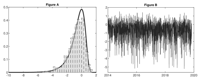
Figure 5.1: Histogram and time-series plot of $\textsf{log}|\hat{Z}_{t}|$

6 Conclusion

We derive the asymptotic properties of an SMM estimator of the unknown parameter vector governing a factor copula model with estimable factors and show how to estimate its limiting variance-covariance matrix consistently. The asymptotic theory is derived from primitive conditions, thereby complementing also the earlier work of Oh and Patton (2013), whose model is nested in our framework. One avenue for future resarch that can be pursued is to consider quasi-Bayesian estimation to alleviate the difficulties of having to deal with a non-smooth objective function. For example, the sample criterion function considered may be shown to fulfill the regularity conditions needed for Laplace-type estimation in Chernozhukov and Hong (2003, section 4.1); see also Hong et al. (2021) for a recent application of this idea to an SMM objective function with overlapping simulation draws.

Appendix A Technical Appendix

Preliminaries: To begin with, suppose $i,j\in\mathcal{G}_{q}$ for $1\leq i<j\leq n$ and some $q\in\{1,\dots,Q\}$. Next, define the empirical copulae

$$\begin{split}\hat{\textsf{C}\,}_{T,S,i,j}(u_{i}&,u_{j};\,\theta_{q},\nu)\\ \coloneqq&\,\frac{1}{TS}\sum_{t\,=\,1}^{T}\sum_{s\,=\,1}^{S}1\{\hat{X}_{i,t,s}(\theta_{q},\nu)\leq\hat{\textsf{G}\,}_{T,S,i}^{-}(u_{i};\theta_{q},\nu),\hat{X}_{j,t,s}(\theta_{q},\nu)\leq\hat{\textsf{G}\,}_{T,S,j}^{-}(u_{j};\theta_{q},\nu)\}\end{split}$$ (A.1)

and

$$\hat{\textsf{C}\,}_{T,i,j}(u_{i},u_{j};\lambda)\coloneqq\,\frac{1}{T}\sum_{t\,=\,1}^{T}1\{\hat{\eta}_{i,t}(\lambda)\leq\hat{\textsf{F}\,}_{T,i}^{-}(u_{i};\lambda),\hat{\eta}_{j,t}(\lambda)\leq\hat{\textsf{F}\,}_{T,j}^{-}(u_{j};\lambda)\},$$ (A.2)

where $\theta_{q}=(\alpha_{q}^{\prime},\beta_{q}^{\prime},\gamma^{\prime},\delta^{\prime})^{\prime}\in\Theta$, $u_{i},u_{j}\in[0,1]$, while $\nu\in\mathcal{U}(\nu_{0})$ and $\lambda\in\mathcal{U}(\lambda_{0})$, with $\mathcal{U}(\cdot)$ denoting neighborhoods around a given parameter as defined by Assumption E. Below, we make frequently use of the identities [see, e.g., Tsukahara (2005) and Segers (2012)]:

$$\begin{split}\hat{\textsf{C}\,}_{T,S,i,j}(u_{i},u_{j};\,\theta_{q},\nu)=\,&\tilde{\textsf{C}}_{T,S,i,j}\{\tilde{\textsf{C}}_{T,S,i}^{-}(u_{i};\theta_{q},\nu),\tilde{\textsf{C}}_{T,S,j}^{-}(u_{j};\theta_{q},\nu);\theta_{q},\nu\}\\ \hat{\textsf{C}\,}_{T,i,j}(u_{i},u_{j};\,\lambda)=\,&\tilde{\textsf{C}}_{T,i,j}\{\tilde{\textsf{C}}_{T,i}^{-}(u_{i};\lambda),\tilde{\textsf{C}}_{T,j}^{-}(u_{j};\lambda);\lambda\},\end{split}$$ (A.3)

where

$$\begin{split}\tilde{\textsf{C}}_{T,S,i,j}(u_{i},u_{j};\theta_{q},\nu)\coloneqq\,&\frac{1}{TS}\sum_{t\,=\,1}^{T}\sum_{s\,=\,1}^{S}1\{\hat{X}_{i,t,s}(\theta_{q},\nu)\leq\textsf{G}_{q}^{-1}(u_{i};\theta_{q}),\hat{X}_{j,t,s}(\theta_{q},\nu)\leq\textsf{G}_{q}^{-1}(u_{j};\theta_{q})\}\\ \tilde{\textsf{C}}_{T,i,j}(u_{i},u_{j};\lambda)\coloneqq\,&\frac{1}{T}\sum_{t\,=\,1}^{T}1\{\hat{\eta}_{i,t}(\lambda)\leq\textsf{F}_{i}^{-1}(u_{i}),\hat{\eta}_{j,t}(\lambda)\leq\textsf{F}_{j}^{-1}(u_{j})\},\end{split}$$ (A.4)

and $\tilde{\textsf{C}}_{T,S,k}(u_{i};\theta_{q},\nu)=\tilde{\textsf{C}}_{T,S,i,j}(\vec{u}_{k};\theta_{q},\nu)$, $\tilde{\textsf{C}}_{T,k}(u_{k};\lambda)=\tilde{\textsf{C}}_{T,i,j}(\vec{u}_{k};\lambda)$, with $\vec{u}_{i}=(u_{i},1)^{\prime}$, $\vec{u}_{j}=(1,u_{j})^{\prime}$. Moreover, define the non-centered processes

$$\begin{split}\hat{\mathbb{C}}_{T,S,i,j}(u_{i},u_{j};\theta_{q},\nu)\coloneqq\,&\sqrt{T}(\hat{\textsf{C}\,}_{T,S,i,j}(u_{i},u_{j};\theta_{q},\nu)-\textsf{C}_{q}(u_{i},u_{j};\theta_{q}))\\ \hat{\mathbb{C}}_{T,i,j}(u_{i},u_{j};\lambda)\coloneqq\,&\sqrt{T}(\hat{\textsf{C}\,}_{T,i,j}(u_{i},u_{j};\lambda)-\textsf{C}_{q}(u_{i},u_{j})),\end{split}$$ (A.5)

and the centered processes

$$\begin{split}\tilde{\mathbb{C}}_{T,S,i,j}(u_{i},u_{j};\theta_{q},\nu)\coloneqq\,&\sqrt{T}(\tilde{\textsf{C}}_{T,S,i,j}(u_{i},u_{j};\theta_{q},\nu)-\textsf{E}[\tilde{\textsf{C}}_{T,S,i,j}(u_{i},u_{j};\theta_{q},\nu)])\\ \tilde{\mathbb{C}}_{T,i,j}(u_{i},u_{j};\lambda)\coloneqq\,&\sqrt{T}(\tilde{\textsf{C}}_{T,i,j}(u_{i},u_{j};\lambda)-\textsf{E}[\tilde{\textsf{C}}_{T,i,j}(u_{i},u_{j};\lambda)]).\end{split}$$ (A.6)

A.1 Proof of Proposition 1

Proof of Proposition 1 ($a$): Recall the definition of the population rank statistics from Eq. (3.16) and note that

$$\psi_{q,k}=\int_{[0,1]^{2}}\varphi_{k}(u_{i},u_{j})\textsf{d}\textsf{C}_{q}(u_{i},u_{j}),\;\;\psi_{q,k}(\theta)=\int_{[0,1]^{2}}\varphi_{k}(u_{i},u_{j})\textsf{d}\textsf{C}_{q}(u_{i},u_{j};\theta_{q})$$

for any $i,j\in\mathcal{G}_{q}$, $q\in\{1,\dots,Q\}$. Hence, one gets, in view of Lemma 3 and Lemma 4, the following representation

$$\sqrt{T}(\hat{\psi}_{T,i,j,k}(\hat{\lambda}_{T})-\psi_{q,k})=\int_{[0,1]^{2}}\hat{\mathbb{C}}_{T,i,j}(u_{i},u_{j})\textsf{d}\varphi_{k}(u_{i},u_{j})+o_{p}(1),$$ (A.7)

with $\hat{\mathbb{C}}_{T,i,j}(u_{i},u_{j})\coloneqq\sqrt{T}(\hat{\textsf{C}\,}_{T,i,j}(u_{i},u_{j})-\textsf{C}_{q}(u_{i},u_{j}))$, and, uniformly in $\theta\in\Theta$,

$$\sqrt{T}(\hat{\psi}_{T,S,i,j,k}(\theta_{q},\hat{\nu}_{T})-\psi_{q,k}(\theta))=\int_{[0,1]^{2}}\hat{\mathbb{C}}_{T,S,i,j}(u_{i},u_{j};\theta_{q})\textsf{d}\varphi_{k}(u_{i},u_{j})+o_{p}(1),$$ (A.8)

with $\hat{\mathbb{C}}_{T,S,i,j}(u_{i},u_{j};\theta_{q})\coloneqq\sqrt{T}(\hat{\textsf{C}\,}_{T,S,i,j}(u_{i},u_{j};\theta_{q})-\textsf{C}_{q}(u_{i},u_{j};\theta_{q}))$, $\hat{\textsf{C}\,}_{T,i,j}(u_{i},u_{j})\coloneqq\hat{\textsf{C}\,}_{T,i,j}(u_{i},u_{j};\lambda_{0})$, $\hat{\textsf{C}\,}_{T,S,i,j}(u_{i},u_{j};\theta_{q})\coloneqq\hat{\textsf{C}\,}_{T,S,i,j}(u_{i},u_{j};\theta,\nu_{0})$; see Eqs. (A.1) and (A.2). Thus, the claim is due to the weak convergence of $\hat{\mathbb{C}}_{T,i,j}$ and $\hat{\mathbb{C}}_{T,S,i,j}$. To see this, note that the functional delta method [cf. van der Vaart and Wellner (1996, Theorem 3.9.4)] in conjunction with Assumption C and Bücher and Volgushev (2013, Theorem 2.4.) yields

$$\hat{\mathbb{C}}_{T,i,j}(u_{i},u_{j})=\tilde{\mathbb{C}}_{T,i,j}(u_{i},u_{j})-\sum_{k\,\in\,\{i,j\}}\partial_{k}\textsf{C}_{q}(u_{i},u_{j})\tilde{\mathbb{C}}_{T,i,j}(\vec{u}_{k})+R(u_{i},u_{j}),$$ (A.9)

and

$$\begin{split}\hat{\mathbb{C}}_{T,S,i,j}(u_{i},u_{j};\theta_{q})=\,&\tilde{\mathbb{C}}_{T,S,i,j}(u_{i},u_{j};\theta_{q})\\ \,&-\sum_{k\,\in\,\{i,j\}}\partial_{k}\textsf{C}_{q}(u_{i},u_{j};\theta_{q})\tilde{\mathbb{C}}_{T,S,i,j}(\vec{u}_{k};\theta_{q})+R_{1}(u_{i},u_{j};\theta_{q}),\end{split}$$ (A.10)

where $\operatorname*{\textsf{sup}}\limits_{u_{i},u_{j}\,\in\,[0,1]}|R(u_{i},u_{j})|=o_{p}(1)$, $\operatorname*{\textsf{sup}}\limits_{\theta_{q}\,\in\,\Theta}\operatorname*{\textsf{sup}}\limits_{u_{i},u_{j}\,\in\,[0,1]}|R_{1}(u_{i},u_{j};\theta_{q})|=o_{p}(1)$, and $\tilde{\mathbb{C}}_{T,i,j}(u_{i},u_{j})\coloneqq\tilde{\mathbb{C}}_{T,i,j}(u_{i},u_{j};\lambda_{0})$, $\tilde{\mathbb{C}}_{T,S,i,j}(u_{i},u_{j};\theta_{q})\coloneqq\tilde{\mathbb{C}}_{T,S,i,j}(u_{i},u_{j};\theta_{q},\nu_{0})$; see Eq. (A.6). The claim follows from Lemma 1 and Lemma 2.

Proof of Proposition 1 ($b$): Taking Eq. (3.20), Lemma 3, and Lemma 4 into account, one gets

$$\sqrt{T}\hat{\Psi}_{T,S,i,j,k}(\theta_{q},\hat{\lambda}_{T},\hat{\nu}_{T})=\int_{[0,1]^{2}}\hat{\mathbb{B}}_{T,S,i,j}(u_{i},u_{j})\,\textsf{d}\varphi_{k}(u_{i},u_{j})+o_{p}(1),$$ (A.11)

where $\hat{\mathbb{B}}_{T,S,i,j}(u_{i},u_{j})\coloneqq\hat{\mathbb{B}}_{T,S,i,j}(u_{i},u_{j};\theta_{0,q},\lambda_{0},\nu_{0})$. We show next that $\hat{\mathbb{B}}_{T,S,i,j}$ converges weakly to the tight Gaussian process $\mathbb{B}_{S}$ concentrated on $\mathbb{D}_{0}\coloneqq\{\alpha\in C[0,1]^{n}:\alpha(1,\dots,1)=0,\;\alpha(x)=0\text{ if some of the components of $x$ are equal to zero}\}$ by establishing (1) asymptotic tightness and (2) finite dimensional (‘fidi’, henceforth) convergence. (1) Stochastic equicontinuity: The functional delta method yields

$$\hat{\mathbb{B}}_{T,S,i,j}(u_{i},u_{j})=\tilde{\mathbb{B}}_{T,S,i,j}(u_{i},u_{j})-\sum_{k\,\in\,\{i,j\}}\partial_{k}\textsf{C}_{q}(u_{i},u_{j})\tilde{\mathbb{B}}_{T,S,i,j}(\vec{u}_{k})+o_{p}(1),$$ (A.12)

where

$$\tilde{\mathbb{B}}_{T,S,i,j}(u_{i},u_{j})=\frac{1}{\sqrt{T}}\sum_{t\,=\,1}^{T}\frac{1}{S}\sum_{s\,=\,1}^{S}(1\{V_{i,t}\leq u_{i},V_{j,t}\leq u_{j}\}-1\{U_{i,t,s}\leq u_{i},U_{j,t,s}\leq u_{j}\}),$$ (A.13)

with $V_{k,t}\coloneqq\textsf{F}_{k}(\eta_{k,t})$, $U_{k,t,s}\coloneqq\textsf{G}_{q}(X_{k,t,s}(\theta_{0,q});\theta_{0,q})$ for $k\in\{i,j\}$. Let $\xi_{i,j,t,S}=(V_{i,t},V_{j,t},\textsf{U}_{S:i,j,t}^{\prime})^{\prime}$, with $\textsf{U}_{S:i,j,t}\coloneqq(U_{i,t,1},U_{j,t,1},\dots,U_{i,t,S},U_{j,t,S})^{\prime}$. We can view $\tilde{\mathbb{B}}_{T,S,i,j}$ as an empirical process indexed by $\bar{f}\in\bar{\mathcal{F}}$:

$$\bar{\mathcal{F}}\coloneqq\{\xi_{S:i,j,t}\mapsto\bar{f}(\xi_{S:i,j,t})\coloneqq\frac{1}{S}\sum_{s\,=\,1}^{S}(f(V_{i,t},V_{j,t})-f(U_{i,t,s},U_{j,t,s})):f\in\mathcal{F}\},$$ (A.14)

where $\mathcal{F}\coloneqq\big{\{}(x_{1},x_{2})\mapsto 1\{x_{1}\leq u_{1},x_{2}\leq u_{2}\},\,u_{1},u_{2}\in[0,1]\big{\}}$. Clearly, $\bar{\mathcal{F}}$ has envelope 1. We use Theorem 1 below to establish asymptotic equicontinuity. Specifically, the bracketing number $\mathcal{N}_{[\,]}(\epsilon,\bar{\mathcal{F}},\rho(\cdot))$, with $\rho(\bar{f})\coloneqq\operatorname*{\textsf{sup}}_{t,T}\lVert\bar{f}(\xi_{i,j,t,S})\rVert_{2}$, shall be determined; see the discussion surrounding theorem 1 for details. It is well-known [see, e.g, van der Vaart (1994, Example 19.6)] that $\mathcal{N}_{[\,]}(\epsilon,\mathcal{F}_{k},\lVert\cdot\rVert_{2})=O(\varepsilon^{-2})$, with $\mathcal{F}_{k}\coloneqq\{x_{k}\mapsto 1\{x_{k}\leq u_{k}\},u_{k}\in[0,1]\}$. Since $\mathcal{F}\subseteq\mathcal{F}_{1}\cdot\mathcal{F}_{2}$, one gets $\mathcal{N}_{[\,]}(\epsilon,\mathcal{F},\lVert\cdot\rVert_{2})=O(\varepsilon^{-4})$; see, e.g., Kosorok (2008, Lemma 9.25). Suppose $[l_{k},u_{k}]$, $k=1,\dots,m\coloneqq\mathcal{N}_{[\,]}(\epsilon,\mathcal{F},\lVert\cdot\rVert_{2})$, represent the brackets needed to cover $\mathcal{F}$. We can then cover $\bar{\mathcal{F}}$ with $[\bar{l}_{k},\bar{u}_{k}]$, $k=1,\dots,m$, where

$$\begin{split}\bar{l}_{k}(\xi_{S:i,j,t})\coloneqq\,&\frac{1}{S}\sum_{s\,=\,1}^{S}(l_{k}(V_{i,t},V_{j,t})-u_{k}(U_{i,t,s},U_{j,t,s}))\\ \bar{u}_{k}(\xi_{S:i,j,t})\coloneqq\,&\frac{1}{S}\sum_{s\,=\,1}^{S}(u_{k}(V_{i,t},V_{j,t})-l_{k}(U_{i,t,s},U_{j,t,s})).\end{split}$$ (A.15)

Note, that $\rho(\bar{u}_{k}-\bar{l}_{k})\leq 2\epsilon$. Thus, $\mathcal{N}_{[\,]}(\epsilon,\bar{\mathcal{F}},\rho(\cdot))=O(\epsilon^{-4})$. Now, since $\{\xi_{i,j,t,S}:t\geq 1\}$ is $i.i.d.$ and $\bar{\mathcal{F}}$ is uniformly bounded, the conditions of Theorem 1 are satisfied. (2) ‘Fidi’-convergence: By the Cramér-Wold device [see, e.g., White (2001, Proposition 5.1)], it suffices to fix some $c\coloneqq(c_{1},\dots,c_{m})^{\prime}\in\mathbb{R}^{m}$, with $\lVert c\rVert=1$, $(\{u_{1},v_{1}\}\dots,\{u_{m},v_{m}\})^{\prime}\in[0,1]^{2m}$, and to consider

$$Z_{T,S}(m)\coloneqq\sum_{l\,=\,1}^{m}c_{l}\tilde{\mathbb{B}}_{T,S,i,j}(u_{l},v_{l})=\frac{1}{\sqrt{T}}\sum_{t\,=\,1}^{T}B_{t,S}(m),$$ (A.16)

where $B_{t,S}(m)\coloneqq\sum_{l\,=\,1}^{m}c_{l}\zeta_{t,S}(u_{l},v_{l})$, with

$$\zeta_{t,S}(u_{l},v_{l})\coloneqq 1\{V_{i,t}\leq u_{l},V_{j,t}\leq v_{l}\}-\frac{1}{S}\sum_{s\,=\,1}^{S}1\{U_{i,t,s}\leq u_{l},U_{j,t,s}\leq v_{l}\}.$$ (A.17)

The sequence $\{B_{t,S}(m):t\geq 1\}$ is $i.i.d$, bounded, and, by Assumption B, centered. It thus follows from White (2001, Theorem 5.11) that $Z_{T,S}(m)\stackrel{{\scriptstyle d}}{{\longrightarrow}}\mathcal{N}(0,\sigma_{S}^{2}(m))$, with $\sigma_{S}^{2}(m)\coloneqq\lim\limits_{T\rightarrow\infty}\sigma_{T,S}^{2}(m)$, provided $\operatorname*{\textsf{inf}}\limits_{T,S\,\geq\,1}\sigma_{T,S}^{2}(m)>0$ for $\sigma_{T,S}^{2}(m)\coloneqq\textsf{var}[Z_{T,S}(m)]$. Now,

$$\sigma_{T,S}^{2}(m)=\sum_{k,l\,=\,1}^{m}c_{k}c_{l}\hat{\gamma}_{T,S}(k,l),\;\;\hat{\gamma}_{T,S}(k,l)\coloneqq\frac{1}{T}\sum_{t,h\,=\,1}^{T}\textsf{cov}[\zeta_{t,S}(w_{k}),\zeta_{t,S}(w_{l})],$$ (A.18)

where $w_{j}\eqqcolon(u_{j},v_{j})^{\prime}\in[0,1]^{2}$, $j\in\{1,\dots,m\}$. Since, $\{\zeta_{t,S}(w_{k}):t\geq 1\}$ is $i.i.d.$, one gets $\hat{\gamma}_{1,S}(k,l)=\textsf{cov}[\zeta_{1,S}(w_{k}),\zeta_{1,S}(w_{l})].$ Next, for any $i,j\in\mathcal{G}_{q}$, $q\in\{1,\dots,Q\}$, one gets

$$\begin{split}\textsf{cov}[\zeta_{1,S}(w_{k}),\zeta_{1,S}(w_{l})\mid Z_{1}]=\,&\textsf{C}_{q,1}(u_{k}\wedge u_{l},v_{k}\wedge v_{l})-\textsf{C}_{q,1}(u_{k},v_{k})\textsf{C}_{q,1}(u_{l},v_{l})\\ \,&+[\mathcal{C}_{q,1}(u_{k}\wedge u_{l},v_{k}\wedge v_{l})-\mathcal{C}_{q,1}(u_{k},v_{k})\mathcal{C}_{q,1}(u_{l},v_{l})]/S,\end{split}$$ (A.19)

where the penultimate equality uses that $\{V_{i,t},V_{j,t}\}\perp\{U_{i,t,s},U_{j,t,s}\}\mid Z_{t}$ and $\{U_{i,t,r},U_{j,t,r}\}\perp\{U_{i,t,s},U_{j,t,s}\}\mid Z_{t}$, $r\neq s$. Since $\textsf{E}[\zeta_{1,S}(w_{k})\mid Z_{1}]=\textsf{C}_{q,1}(w_{k})-\mathcal{C}_{q,1}(w_{k})$, we get, by the law of total covariance,

$$\begin{split}\textsf{cov}[\zeta_{1,S}(w_{k}),\zeta_{1,S}(w_{l})]=\,&\textsf{E}[\textsf{C}_{q,t}(w_{k}\wedge w_{l})-\textsf{C}_{q,t}(w_{k})\textsf{C}_{q,t}(w_{l})]\\ \,&+\textsf{E}[(\textsf{C}_{q,t}(w_{k})-\mathcal{C}_{q,t}(w_{k}))(\textsf{C}_{q,t}(w_{l})-\mathcal{C}_{q,t}(w_{l}))]\\ \,&+\textsf{E}[\mathcal{C}_{q,t}(w_{k}\wedge w_{l})-\mathcal{C}_{q,t}(w_{k})\mathcal{C}_{q,t}(w_{l})]/S\\ \eqqcolon\,&\gamma^{(1)}_{q}(k,l)+\gamma^{(2)}_{q}(k,l)+\gamma^{(3)}_{q}(k,l)/S,\end{split}$$

say. We are left with showing

$$\sigma_{T,S}^{2}(m)\coloneqq\sigma_{S}^{2}(m)=c^{\prime}(\gamma^{(1)}_{q}(k,l))_{1\leq k,l\leq m}c+c^{\prime}(\gamma^{(2)}_{q}(k,l))_{1\leq k,l\leq m}c/S+c^{\prime}(\gamma^{(3)}_{q}(k,l))_{1\leq k,l\leq m}c>0.$$

Clearly, if $\textsf{C}_{q,t}(w_{1}),\dots,\textsf{C}_{q,t}(w_{m})$ are all distinct $a.s.$ and $\mathcal{C}_{q,t}(w_{1}),\dots,\mathcal{C}_{q,t}(w_{m})$ are all distinct $a.s.$ with values in $(0,1)$ $a.s.$, then the claim follows by Assumption F. For the cases where not all are distinct or take values in $\{0,1\}$ the claim follows from the argument used in the proof of Boistard et. al (2017, Lemma 9.6). Therefore, combining (1) and (2) yields $\tilde{\mathbb{B}}_{T,S,i,j}(u,v)\rightsquigarrow\mathbb{C}_{q,S}(u,v)$, so that

$$\sqrt{T}\hat{\Psi}_{T,S,i,j,k}(\theta,\hat{\lambda}_{T},\hat{\nu}_{T})\stackrel{{\scriptstyle d}}{{\longrightarrow}}\mathcal{N}(0,\sigma_{0,S}(q,q\mid k,k)),$$

with

$$\sigma_{0,S}(q,q\mid k,k)\coloneqq\int_{[0,1]^{2}}\int_{[0,1]^{2}}\textsf{E}[\mathbb{C}_{q,S}(u_{1},v_{1})\mathbb{C}_{q,S}(u_{2},v_{2})]\textsf{d}\varphi_{k}(u_{1},v_{1})\textsf{d}\varphi_{k}(u_{2},v_{2});$$

see also Berghaus et al. (2017, Theorem 3.3). To conclude from here, use that $\{\hat{\mathbb{B}}_{T,S,i,j}(u_{i},u_{j}):1\leq i<j\leq n\}$ are jointly normal as $T\rightarrow\infty$. To see this, note that $\hat{\mathbb{B}}_{T,S,i,j}(u_{i},u_{j})=\hat{\mathbb{B}}_{T,S}(\vec{u}_{i,j})$, where $\vec{u}_{i,j}$ denotes the $n$-dimensional vector of ones with $u_{i}$ ($u_{j}$) at $i$-th ($j$-th) position and $\tilde{\mathbb{B}}_{T,S}(u_{1},\dots,u_{n})=\hat{\mathbb{B}}_{T,S}(u_{1},\dots,u_{n};\theta_{0},\lambda_{0},\nu_{0})$, with

$$\begin{split}\hat{\mathbb{B}}_{T,S}(u_{1},&\dots,u_{n};\theta,\lambda,\nu)\\ \coloneqq\,&\frac{1}{\sqrt{T}}\sum_{t\,=\,1}^{T}\big{[}1\{\hat{\eta}_{1,t}(\lambda_{1})\leq\textsf{F}_{1,T}^{-}(u_{1};\lambda_{1}),\dots,\hat{\eta}_{n,t}(\lambda_{n})\leq\textsf{F}_{n,T}^{-}(u_{n};\lambda_{n})\}\\ \,&\hskip 21.33955pt-\frac{1}{S}\sum_{s\,=\,1}^{S}1\{\hat{X}_{1,t,s}(d_{1},\hat{\nu}_{T})\leq G_{1}^{-1}(u_{1};d_{1},\nu),\dots,\hat{X}_{n,t,s}(d_{n},\nu)\leq G_{n}^{-1}(u_{n};d_{n},\nu)\}\big{]}.\end{split}$$

Weak convergence of $\tilde{\mathbb{B}}_{T,S}(u_{1},\dots,u_{n})$ follows by the same arguments used to establish weak convergence of $\tilde{\mathbb{B}}_{T,S,i,j}(u_{i},u_{j})$. Since $n$ is finite, the claim follows.

Proof of Proposition 1 ($c$): Note that we can restrict the event inside the probability to the case where $\hat{\nu}_{T}$ lies in a $\sqrt{T}$ neighborhood of $\nu_{0}$. To see this, recall from Assumption E that $\sqrt{T}\lVert\hat{\nu}_{T}-\nu_{0}\rVert=O_{p}(1)$; i.e., there exists some constant $K\coloneqq K(\varepsilon)<\infty$, independent of $T$, such that $\operatorname*{\overline{\textsf{lim}}}\limits_{T\rightarrow\infty}\textsf{P}(\hat{\nu}_{T}\notin\mathcal{V}_{K,T})<\epsilon$ for any $\epsilon>0$, where

$$\mathcal{V}_{K,T}\coloneqq\{\nu\in\mathcal{V}_{0}:\lVert\nu-\nu_{0}\rVert\leq K/\sqrt{T}\}.$$ (A.20)

Clearly, for sufficiently large $T$, $\mathcal{V}_{K,T}\subseteq\mathcal{U}(\lambda_{0})$, where the neighborhood has been defined in Assumption E. Hence,

$$\begin{split}\operatorname*{\overline{\textsf{lim}}}\limits_{T\rightarrow\infty}&\textsf{P}\bigg{[}\operatorname*{\textsf{sup}}\limits_{\theta,\tilde{\theta}\,\in\,\Theta:\lVert\theta-\tilde{\theta}\rVert\,\leq\,\delta}\sqrt{T}\lVert\hat{\psi}_{T,S}(\theta,\hat{\nu}_{T})-\psi(\theta)-\hat{\psi}_{T,S}(\tilde{\theta},\hat{\nu}_{T})+\psi(\tilde{\theta})\rVert>\eta\bigg{]}\\ &\leq\operatorname*{\overline{\textsf{lim}}}\limits_{T\rightarrow\infty}\textsf{P}(\hat{\nu}_{T}\notin\mathcal{V}_{K,T})\\ &\hskip 14.22636pt+\operatorname*{\overline{\textsf{lim}}}\limits_{T\rightarrow\infty}\textsf{P}\bigg{[}\Big{\{}\operatorname*{\textsf{sup}}\limits_{\theta_{1},\theta_{2}\,\in\,\Theta:\lVert\theta-\tilde{\theta}\rVert\,\leq\,\delta}\sqrt{T}\lVert\hat{\psi}_{T,S}(\theta,\nu_{T})-\psi(\theta)-\hat{\psi}_{T,S}(\tilde{\theta},\nu_{T})+\psi(\tilde{\theta})\rVert>\eta\Big{\}}\,\cap\,\big{\{}\hat{\nu}_{T}\in\mathcal{V}_{K,T}\big{\}}\bigg{]}\\ &\leq\epsilon+\operatorname*{\overline{\textsf{lim}}}\limits_{T\rightarrow\infty}\textsf{P}\bigg{[}\operatorname*{\textsf{sup}}\limits_{\nu\,\in\,\mathcal{V}_{K,T},\,\theta,\tilde{\theta}\,\in\,\Theta:\lVert\theta-\tilde{\theta}\rVert\,\leq\,\delta}\sqrt{T}\lVert\hat{\psi}_{T,S}(\theta,\nu)-\psi(\theta)-\hat{\psi}_{T,S}(\tilde{\theta},\nu)+\psi(\tilde{\theta})\rVert>\eta\bigg{]}.\end{split}$$

Since, by Lemma 3 and Lemma 4, one has

$$\operatorname*{\overline{\textsf{lim}}}\limits_{T\rightarrow\infty}\textsf{P}\bigg{[}\operatorname*{\textsf{sup}}\limits_{\nu\,\in\,\mathcal{V}_{K,T}}\operatorname*{\textsf{sup}}\limits_{\theta\,\in\,\Theta}\sqrt{T}\lVert\hat{\psi}_{T,S}(\theta,\nu)-\hat{\psi}_{T,S}(\theta,\nu_{0})\rVert>\eta\bigg{]}<\epsilon,$$

it suffices to show that

$$\operatorname*{\overline{\textsf{lim}}}\limits_{T\rightarrow\infty}\textsf{P}\bigg{[}\operatorname*{\textsf{sup}}\limits_{\theta,\tilde{\theta}\,\in\,\Theta:\lVert\theta-\tilde{\theta}\rVert\,\leq\,\delta}\sqrt{T}\lVert\hat{\psi}_{T,S}(\theta,\nu_{0})-\psi(\theta)-\hat{\psi}_{T,S}(\tilde{\theta},\nu_{0})+\psi(\tilde{\theta})\rVert>\eta\bigg{]}<\epsilon.$$ (A.21)

To begin with, recall that $\theta_{q}=(\alpha_{q}^{\prime},\beta_{q}^{\prime},\gamma^{\prime},\delta^{\prime})^{\prime}$, $q=1,\dots,Q$. Thus, by a slight abuse of notation, $\theta=(\alpha_{1}^{\prime},\beta_{1}^{\prime},\dots,\alpha_{Q}^{\prime},\beta_{Q}^{\prime},\gamma^{\prime},\delta^{\prime})^{\prime}=\cup_{q\,=\,1}^{Q}\theta_{q}$. Therefore, by the triangle inequality

$$\begin{split}\lVert&\hat{\psi}_{T,S}(\theta,\nu_{0})-\psi(\theta)-\hat{\psi}_{T,S}(\tilde{\theta},\nu_{0})+\psi(\tilde{\theta})\rVert\\ &\leq\sum_{q\,=\,1}^{Q}\frac{1}{\displaystyle{|\mathcal{G}_{q}|\choose 2}}\mathop{\sum\sum}\limits_{\begin{subarray}{c}1\leq i<j\leq n\\ i,j\,\in\,\mathcal{G}_{q}\end{subarray}}\sum_{k\,=\,1}^{\ell}|\hat{\psi}_{T,S,i,j,k}(\theta_{q},\nu_{0})-\psi_{q,k}(\theta_{q})-\hat{\psi}_{T,S,i,j,k}(\tilde{\theta}_{q},\nu_{0})+\psi_{q,k}(\tilde{\theta}_{q})|.\end{split}$$

Hence,

$$\begin{split}\textsf{P}\bigg{[}&\operatorname*{\textsf{sup}}\limits_{\theta,\tilde{\theta}\,\in\,\Theta:\lVert\theta-\tilde{\theta}\rVert\,\leq\,\delta}\sqrt{T}\lVert\hat{\psi}_{T,S}(\theta,\nu_{0})-\psi(\theta)-\hat{\psi}_{T,S}(\tilde{\theta},\nu_{0})+\psi(\tilde{\theta})\rVert>\eta\bigg{]}\\ &\hskip 7.11317pt\leq\sum_{q\,=\,1}^{Q}\mathop{\sum\sum}\limits_{\begin{subarray}{c}1\leq i<j\leq n\\ i,j\,\in\,\mathcal{G}_{q}\end{subarray}}\sum_{k\,=\,1}^{\ell}\textsf{P}\bigg{[}\operatorname*{\textsf{sup}}\limits_{\theta_{q},\tilde{\theta}_{q}\,\in\,\Theta:\lVert\theta-\tilde{\theta}\rVert\,\leq\,\delta}|\hat{\psi}_{T,S,i,j,k}(\theta_{q},\nu_{0})-\psi_{q,k}(\theta_{q})\\ &\hskip 213.39566pt-\hat{\psi}_{T,S,i,j,k}(\tilde{\theta}_{q},\nu_{0})+\psi_{q,k}(\tilde{\theta}_{q})|>\frac{\eta}{Q\ell}\bigg{]}.\end{split}$$

Now, suppose $i,j\in\mathcal{G}_{q}$ for some $q\in\{1,\dots,Q\}$. Moreover, let us recall from Eq. (A.8) that uniformly in $\theta_{q}\in\Theta$

$$\begin{split}\sqrt{T}|\hat{\psi}_{T,S,i,j,k}(\theta_{q},\nu_{0})-&\psi_{q,k}(\theta_{q})|\\ &\leq\,\left|\int_{[0,1]^{2}}\textsf{d}\varphi_{k}(u_{i},u_{j})\right|\operatorname*{\textsf{sup}}\limits_{u_{i},u_{j}\,\in\,[0,1]}|\hat{\mathbb{C}}_{i,j,T,S}(u_{i},u_{j};\theta_{q})|+|R(\theta_{q})|\end{split}$$ (A.22)

for $1\leq i<j\leq n$ and $k\in\{1,\dots,\ell\}$, where $\operatorname*{\textsf{sup}}\limits_{\theta\,\in\,\Theta}|R(\theta_{q})|=o_{p}(1)$. Since $n$ and $\ell$ are fixed, we are left with showing that for any $\epsilon,\eta>0$, there exists some $\delta>0$ such that

$$\begin{split}\operatorname*{\overline{\textsf{lim}}}\limits_{T\rightarrow\infty}\textsf{P}\bigg{[}\operatorname*{\textsf{sup}}\limits_{\theta_{q},\tilde{\theta}_{q}\,\in\,\Theta:\lVert\theta_{q}-\tilde{\theta}_{q}\rVert\,\leq\,\delta}\operatorname*{\textsf{sup}}\limits_{u_{i},u_{j}\,\in\,[0,1]}|\hat{\mathbb{C}}_{T,S,i,j}(u_{i},u_{j};\theta_{q})-\hat{\mathbb{C}}_{T,S,i,j}(u_{i},u_{j};\tilde{\theta}_{q})|>\eta\bigg{]}<\epsilon.\end{split}$$ (A.23)

In view of Eqs. (A.3) and (A.4), we see that

$$\begin{split}\hat{\mathbb{C}}_{T,S,i,j}(u_{i},u_{j};\theta_{q})=\,&\sqrt{T}(\tilde{\textsf{C}}_{T,S,i,j}\{\tilde{\textsf{C}}_{T,S,i}^{-}(u_{i};\theta_{q}),\tilde{\textsf{C}}_{T,S,j}^{-}(u_{j};\theta_{q});\theta_{q}\}-\textsf{C}_{i,j}\{\tilde{\textsf{C}}_{T,S,i}^{-}(u_{i};\theta_{q}),\tilde{\textsf{C}}_{T,S,j}^{-}(u_{j};\theta_{q});\theta_{q}\})\\ \,&+\sqrt{T}(\textsf{C}_{i,j}\{\tilde{\textsf{C}}_{T,S,i}^{-}(u_{i};\theta_{q}),\tilde{\textsf{C}}_{T,S,j}^{-}(u_{j};\theta_{q});\theta_{q}\}-\textsf{C}_{q}(u_{i},u_{j})).\end{split}$$

with $\tilde{\textsf{C}}_{T,S,i,j}(u_{i},u_{j};\theta_{q})\coloneqq\tilde{\textsf{C}}_{T,S,i,j}(u_{i},u_{j};\theta,\nu_{0})$ and $\tilde{\textsf{C}}_{T,S,k}^{-}(u_{k};\theta_{q})\coloneqq\tilde{\textsf{C}}_{T,S,k}^{-}(u_{k};\theta_{q},\nu_{0})$ for $k\in\{i,j\}$. Therefore, using an argument similar that in Tsukahara (2005, Appendix B), one obtains

$$\begin{split}\textsf{P}\bigg{[}&\operatorname*{\textsf{sup}}\limits_{\theta_{q},\tilde{\theta}_{q}\,\in\,\Theta:\lVert\theta_{q}-\tilde{\theta}_{q}\rVert\,\leq\,\delta}\operatorname*{\textsf{sup}}\limits_{u_{i},u_{j}\,\in\,[0,1]}|\hat{\mathbb{C}}_{T,S,i,j}(u_{i},u_{j};\theta_{q})-\hat{\mathbb{C}}_{T,S,i,j}(u_{i},u_{j};\tilde{\theta}_{q})|>\eta\bigg{]}\\ &\leq\,\textsf{P}\bigg{[}\operatorname*{\textsf{sup}}\limits_{\theta_{q},\tilde{\theta}_{q}\,\in\,\Theta:\lVert\theta_{q}-\tilde{\theta}_{q}\rVert\,\leq\,\delta}\operatorname*{\textsf{sup}}\limits_{u_{i},u_{j}\,\in\,[0,1]}|\tilde{\mathbb{C}}_{T,S,i,j}(u_{i},u_{j};\theta_{q})-\tilde{\mathbb{C}}_{T,S,i,j}(u_{i},u_{j};\tilde{\theta}_{q})|>\frac{\eta}{2}\bigg{]}\\ &\hskip 5.69046pt+\sum_{k\in\{i,j\}}\textsf{P}\bigg{[}\operatorname*{\textsf{sup}}\limits_{\theta_{q},\tilde{\theta}_{q}\,\in\,\Theta:\lVert\theta_{q}-\tilde{\theta}_{q}\rVert\,\leq\,\delta}\operatorname*{\textsf{sup}}\limits_{u_{k}\,\in\,[0,1]}|\tilde{\mathbb{C}}_{T,S,i,j}(\vec{u}_{k};\theta_{q})-\tilde{\mathbb{C}}_{T,S,i,j}(\vec{u}_{k};\tilde{\theta}_{q})|>\frac{\eta}{4}\bigg{]}.\end{split}$$ (A.24)

The claim thus follows from part ($c$) of Lemma 2.

A.2 Proof of Corollary 1

Proof of Corollary 1: As argued in Cheng (2015, Lemma 1), it suffices to show that the conditional distribution of $\sqrt{T}(\hat{\Psi}_{T,S}^{(b)}(\hat{\theta}_{T,S},\hat{\lambda}_{T},\hat{\nu}_{T})-\hat{\Psi}_{T,S}(\hat{\theta}_{T,S},\hat{\lambda}_{T},\hat{\nu}_{T}))$ converges in probability to the limiting distribution of $\sqrt{T}\hat{\Psi}_{T,S}(\theta_{0},\hat{\lambda}_{T},\hat{\nu}_{T})$ given in Proposition 1. Specifically, define for any $1\leq i<j\leq n$, with $i,j\in\mathcal{G}_{q}$, $q\in\{1,\dots,Q\}$:

$$\begin{split}\sqrt{T}(\hat{\Psi}_{T,S,i,j}^{(b)}(\hat{\theta}_{T,S,q},\hat{\lambda}_{T},\hat{\nu}_{T})-&\hat{\Psi}_{T,S,i,j}(\hat{\theta}_{T,S,q},\hat{\lambda}_{T},\hat{\nu}_{T}))\\ =&\,\hat{\xi}_{T,S,i,j}^{(b)}(\theta_{0,q},\hat{\lambda}_{T},\hat{\nu}_{T})\\ &\,+\hat{\xi}_{T,S,i,j}^{(b)}(\hat{\theta}_{T,S,q},\hat{\lambda}_{T},\hat{\nu}_{T})-\hat{\xi}_{i,j,T,S}^{(b)}(\theta_{0,q},\hat{\lambda}_{T},\hat{\nu}_{T}),\end{split}$$

where

$$\begin{split}\hat{\xi}_{T,S,i,j}^{(b)}(\hat{\theta}_{T,S,q},\hat{\lambda}_{T},\hat{\nu}_{T})\coloneqq\sqrt{T}(\hat{\Psi}_{T,S,i,j}^{(b)}(\hat{\theta}_{T,S,q},\hat{\lambda}_{T},\hat{\nu}_{T})-\hat{\Psi}_{i,j,T,S}(\hat{\theta}_{T,S,q},\hat{\lambda}_{T},\hat{\nu}_{T}))\end{split}$$ (A.25)

represents the bootstrap analogue of

$$\hat{\xi}_{T,S,i,j}(\hat{\theta}_{T,S,q},\hat{\lambda}_{T},\hat{\nu}_{T})=\sqrt{T}(\hat{\Psi}_{T,S,i,j}(\hat{\theta}_{T,S,q},\hat{\lambda}_{T},\hat{\nu}_{T})-\Psi_{T,S,i,j}(\hat{\theta}_{T,S,q})).$$ (A.26)

We proceed in two steps: 1) the conditional distribution of $\hat{\xi}_{T,S,i,j}^{(b)}(\theta_{0,q},\hat{\lambda}_{T},\hat{\nu}_{T})$ converges in probability to that of $\hat{\xi}_{T,S,i,j}(\theta_{0,q},\hat{\lambda}_{T},\hat{\nu}_{T})=\sqrt{T}\hat{\Psi}_{T,S,i,j}(\theta_{0,q},\hat{\lambda}_{T},\hat{\nu}_{T})$; 2) $\hat{\xi}_{T,S,i,j}^{(b)}(\hat{\theta}_{T,S,q},\hat{\lambda}_{T},\hat{\nu}_{T})-\hat{\xi}_{T,S,i,j}^{(b)}(\theta_{0,q},\hat{\lambda}_{T},\hat{\nu}_{T})=o_{p}(1)$. Step 1): Mimicking the derivation of Eq. (3.20), note that the $k$-th element of $\hat{\xi}_{T,S,i,j}^{(b)}(\theta_{0,q},\hat{\lambda}_{T},\hat{\nu}_{T})$ can be written as:

$$\int_{[0,1]^{2}}(\hat{\mathbb{B}}_{T,S,i,j}^{(b)}-\hat{\mathbb{B}}_{T,S,i,j})(u_{i},u_{j};\theta_{0,q},\lambda_{0},\nu_{0})\,\textsf{d}\varphi_{k}(u_{i},u_{j})+o_{p}(1),$$

where $\hat{\mathbb{B}}_{T,S,i,j}^{(b)}$ is the bootstrap analogue of $\hat{\mathbb{B}}_{T,S,i,j}$ defined in Eq. (3.19). We are thus left with showing that the conditional distribution of $\hat{\mathbb{B}}_{T,S,i,j}^{(b)}-\hat{\mathbb{B}}_{T,S,i,j}$ converges weakly in probability to the same limiting process that governs the weak limit of $\hat{\mathbb{B}}_{T,S,i,j}$. But, by the functional delta method, this is due the weak convergence of $\hat{\mathbb{B}}_{T,S,i,j}$; see the proof of Proposition 1 in conjunction with Fermanian et al. (2004, Theorem 5). Step 2): We can deduce the bootstrap stochastic equicontinuity of (A.25) from that of (A.26) established in Proposition 1 ($c$); see also Giné and Zinn (1990), Brown and Wegkamp (2002), or Chen et al. (2003) for a similar argument. The claim then follows because, by Proposition 2, $\sqrt{T}\lVert\hat{\theta}_{T,S}-\theta_{0}\rVert=O_{p}(1)$.

Appendix B Auxiliary results

This section contains auxiliary results. We make frequently use of the following stochastic equicontinuity result due to Andrews and Pollard (1994, Theorem 2.2):

Theorem 1

For any $T$, let $\{\xi_{t,T}:t=1,\dots,T;\,T\in\mathbb{N}_{1}\}$ be a strong mixing triangular array whose mixing coefficients satisfy

$$\sum_{i\,=\,1}^{\infty}i^{p-2}\alpha(i)^{\theta/(p+\theta)}<\infty i$$ ()

for $p\geq 2$, $p\in\mathbb{N}$, and $\theta>0$, and let $\mathcal{F}$ be a uniformly bounded class of real-valued functions whose bracketing number satisfies

$$\int_{0}^{1}x^{-\theta/(2+\theta)}\mathcal{N}_{[\,]}(x,\mathcal{F},\rho(\cdot))^{1/p}\,\textsf{d}x<\infty, ii$$ ()

for the same $p$ and $\theta$, while $\rho(f)\coloneqq\operatorname*{\textsf{sup}}_{t,T}\lVert f(\xi_{t,T})\rVert_{2}$. Then for each $\epsilon_{0}>0$ there is a $\epsilon_{1}>0$ such that

$$\operatorname*{\overline{\textsf{lim}}}\limits_{T\rightarrow\infty}\left\lVert\operatorname*{\textsf{sup}}_{\rho(f-g)<\epsilon_{1}}\left|\frac{1}{\sqrt{T}}\sum_{t\,=\,1}^{T}[f(\xi_{t,T})-g(\xi_{t,T})]\right|\right\rVert_{p}<\epsilon_{0}. \ast\ast$$ ()

Remark 1

Note that $\int_{0}^{1}1/x^{c}\text{d}x<\infty$ for $c<1$. Thus, if $\alpha(i)=O(i^{-a})$ and $\mathcal{N}_{[\,]}(x,\mathcal{F},\rho(\cdot))=O(i^{-b})$ for $a,b>0$, then ($i$) and ($ii$) are satisfied if $p>b(2+\theta)/2$ and $a>(p-1)(p+\theta)/\theta$ so that $p\geq 2$ and $p\in\mathbb{N}$.

Recall that the bracketing number $\mathcal{N}_{[\,]}(\varepsilon,\mathcal{F},\rho)$ denotes the minimum number of $\varepsilon$-brackets needed to cover a class $\mathcal{F}$ of functions $f:\mathcal{X}\mapsto\mathbb{E}$ equipped with a metric $\rho$:

$$\mathcal{N}_{[\,]}(\varepsilon,\mathcal{F},\rho)\coloneqq\operatorname*{\textsf{min}}\{m:\exists\,(\{l_{j},u_{j}\})_{j=1}^{m}\text{ s.th. }\rho(u_{j},l_{j})\leq\varepsilon,\,\mathcal{F}\subseteq\bigcup_{j\,=\,1}^{m}[l_{j},u_{j}]\},$$ (B.1)

where the bracket $[l_{j},u_{j}]$ is defined by

$$[l_{j},u_{j}]\coloneqq\{f\in\mathcal{F}:l_{j}(x)\leq h(x)\leq u_{j}(x),\forall x\in\mathcal{X}\},$$

see, e.g. van der Vaart and Wellner (1996).

Remark 2

Let $k$ and $K$ be constants independent of $T$, and define

$$\mathcal{V}_{k,T}\coloneqq\{\nu\in\mathcal{V}_{0}:\lVert\nu-\nu_{0}\rVert\leq k/\sqrt{T}\},\quad\Lambda_{K,T}\coloneqq\{\lambda\in\Lambda_{0}:\lVert\lambda-\lambda_{0}\rVert\leq K/\sqrt{T}\}$$ (B.2)

Then, by Assumption E, for $T$ sufficiently large and any $\epsilon>0$, there exist $k\coloneqq k(\epsilon)$, $K\coloneqq K(\epsilon)$, such that $\operatorname*{\overline{\textsf{lim}}}\limits_{T\rightarrow\infty}\textsf{P}(\hat{\nu}_{T}\notin\mathcal{V}_{k,T})<\epsilon$ and $\operatorname*{\overline{\textsf{lim}}}\limits_{T\rightarrow\infty}\textsf{P}(\hat{\lambda}_{T}\notin\Lambda_{K,T})<\epsilon$. For brevity, we write $\mathcal{V}_{T}\coloneqq\mathcal{V}_{k,T}$ and $\Lambda_{T}\coloneqq\Lambda_{K,T}$.

Lemma 1

For any $1\leq i<j\leq n$ with $i,j\in\mathcal{G}_{q}$, $q\in\{1,\dots,Q\}$,

1. $\{\tilde{\mathbb{C}}_{T,i,j}(u_{i},u_{j};\lambda):\,u_{i},u_{j}\in[0,1],\,\lambda\in\Lambda_{T}\}$ is stochastically equicontinuous;

2. Let $\tilde{\mathbb{V}}_{T,i,j}(u_{i},u_{j};\lambda)\coloneqq\sqrt{T}(\tilde{\textsf{C}}_{T,i,j}(u_{i},u_{j};\lambda)-\tilde{\textsf{C}}_{T,i,j}(u_{i},u_{j};\lambda_{0}))$. Then,

   $$\tilde{\mathbb{V}}_{T}(u_{i},u_{j};\lambda)=\bar{\mathbb{V}}_{T}(u_{i},u_{j};\lambda)+o_{p}(1),$$

   uniformly in $u_{i},u_{j}\in[0,1],\lambda\in\Lambda_{T}$, with

   $$\begin{split}\bar{\mathbb{V}}_{T}&(u_{i},u_{j};\lambda)\\ &=\,\sum_{k\,\in\,\{i\textnormal{,}\hskip 0.71114ptj\}}\partial_{k}\textsf{C}_{q}(u_{i},u_{j})\textsf{f}_{k}\{\textsf{F}_{k}^{-1}(u_{k})\}\textsf{E}[\tau_{k}(R_{1},u_{k},\lambda_{0})]\sqrt{T}(\lambda-\lambda_{0})+o_{p}(1),\end{split}$$

   with $\tau_{k}(R_{t};u_{k},\lambda_{0})=\tau_{k}(\mathcal{F}_{t};u_{k},\lambda_{0})$, where for any $\bar{\lambda}\in\mathcal{V}_{T}$

   $$\tau_{k}(\mathcal{F}_{t};u_{k},\bar{\lambda})\coloneqq\frac{\textsf{F}_{k}^{-1}(u_{k})\nabla_{\lambda}\mu_{2,k}(R_{t}(\lambda),\lambda)\big{|}_{\lambda\,=\,\bar{\lambda}}+\nabla_{\lambda}\mu_{1,k}(R_{t}(\lambda),\lambda)\big{|}_{\lambda\,=\,\bar{\lambda}}}{\mu_{k,2}(R_{t},\lambda_{0})},\;\;k\in\{i,j\},$$

   and we recall that $R_{t}=R_{t}(\lambda_{0})$.

3. $\{\tilde{\mathbb{C}}_{T,i,j}(u_{i},u_{j};\lambda_{0}):u_{i},u_{j}\in[0,1]\}$ converges weakly to a tight Gaussian process in $\ell^{\infty}([0,1]^{2})$.

Lemma 2

For any $1\leq i<j\leq n$ with $i,j\in\mathcal{G}_{q}$, $q\in\{1,\dots,Q\}$,

1. $\{\tilde{\mathbb{C}}_{T,S,i,j}(u_{i},u_{j};\theta_{q},\nu):u_{i},u_{j}\in[0,1],\theta_{q}\in\Theta,\nu\in\mathcal{V}_{0}\}$ is stochastically equicontinuous;

2. Let $\tilde{\mathbb{U}}_{T,S,i,j}(u_{i},u_{j};\theta_{q},\nu)\coloneqq\sqrt{T}(\tilde{\textsf{C}}_{T,S,i,j}(u_{i},u_{j};\theta_{q},\nu)-\tilde{\textsf{C}}_{T,S,i,j}(u_{i},u_{j};\theta_{q},\nu_{0}))$. Then, $\tilde{\mathbb{U}}_{T,S}(u_{i},u_{j};\theta_{q},\nu)=\bar{\mathbb{U}}_{T}(u_{i},u_{j};\theta_{q},\nu)+o_{p}(1)$, uniformly in $u_{i},u_{j}\in[0,1],\theta_{q}\in\Theta,\nu\in\mathcal{V}_{T}$, with

   $$\begin{split}\bar{\mathbb{U}}_{T}(u_{i},u_{j};&\theta_{q},\nu)\\ &=\,\beta\textsf{E}[\nabla_{\nu}\sigma(M_{t},\nu_{0})]\sqrt{T}(\nu-\nu_{0})\sum_{k\,\in\,\{i\textnormal{,}\hskip 0.71114ptj\}}\partial_{k}\textsf{C}_{q}(u_{i},u_{j};\theta_{q})\textsf{g}_{q}\{\textsf{G}_{q}^{-1}(u_{k};\theta_{q});\theta_{q}\}+o_{p}(1);\end{split}$$

3. $\{\tilde{\mathbb{C}}_{T,S,i,j}(u_{i},u_{j};\theta,\nu_{0}):u_{i},u_{j}\in[0,1],\theta_{q}\in\Theta\}$ converges weakly to a tight Gaussian process in $\ell^{\infty}([0,1]^{2}\times\Theta)$.

Lemma 3

Set $\hat{\mathbb{V}}_{T,i,j}(u_{i},u_{j};\lambda)\coloneqq\sqrt{T}(\hat{\textsf{C}\,}_{T,i,j}(u_{i},u_{j};\lambda)-\hat{\textsf{C}\,}_{T,i,j}(u_{i},u_{j};\lambda_{0}))$, and define $\hat{\mathbb{U}}_{T,S,i,j}(u_{i},u_{j};\theta_{q},\nu)\coloneqq\sqrt{T}(\hat{\textsf{C}\,}_{T,S,i,j}(u_{i},u_{j};\theta_{q},\nu)-\hat{\textsf{C}\,}_{T,S,i,j}(u_{i},u_{j};\theta_{q},\nu_{0}))$. Then,

$$\textnormal{($a$) }\,\,\operatorname*{\textsf{sup}}\limits_{u_{i},u_{j}\,\in\,[0,1]}|\hat{\mathbb{V}}_{T,i,j}(u_{i},u_{j};\hat{\lambda}_{T})|=o_{p}(1),\;\;\textnormal{($b$) }\,\,\operatorname*{\textsf{sup}}\limits_{\theta_{q}\,\in\,\Theta}\operatorname*{\textsf{sup}}\limits_{u_{i},u_{j}\,\in\,[0,1]}|\hat{\mathbb{U}}_{i,j,T,S}(u_{i},u_{j};\theta_{q},\hat{\nu}_{T})|=o_{p}(1).$$

Lemma 4

For any $k\in\{1,\dots,\ell\}$ and $i,j\in\mathcal{G}_{q}$, $q\in\{1,\dots,Q\}$, we have

$$\begin{split}\sqrt{T}(\hat{\psi}_{T,i,j,k}&(\hat{\lambda}_{T})-\psi_{q,k})\\ \,&=\int_{[0,1]^{2}}\sqrt{T}(\hat{\textsf{C}\,}_{T,i,j}(u_{i},u_{j};\hat{\lambda}_{T})-\textsf{C}_{q}(u_{i},u_{j}))\,\textsf{d}\varphi_{k}(u_{i},u_{j})+o_{p}(1).\end{split} a$$ ()

and, uniformly in $\theta_{q}\in\Theta$,

$$\begin{split}\sqrt{T}(\hat{\psi}_{T,S,i,j,k}&(\theta_{q},\hat{\nu}_{T})-\psi_{q,k}(\theta_{q}))\\ \,&=\int_{[0,1]^{2}}\sqrt{T}(\hat{\textsf{C}\,}_{T,S,i,j}(u_{i},u_{j};\theta_{q},\hat{\nu}_{T})-\textsf{C}_{q}(u_{i},u_{j};\theta_{q}))\,\textsf{d}\varphi_{k}(u_{i},u_{j})+o_{p}(1).\end{split} b$$ ()

B.1 Proof of Lemma 1

Proof of Lemma 1-($a$): To begin with, note that

$$\begin{split}1\{&\hat{\eta}_{i,t}(\lambda)\leq\textsf{F}_{i}^{-1}(u_{i}),\hat{\eta}_{j,t}(\lambda)\leq\textsf{F}_{j}^{-1}(u_{j})\}\\ &=1\{\eta_{i,t}\leq\textsf{F}_{i}^{-1}(u_{i})a_{2,i}^{\dagger}(\mathcal{F}_{t},\lambda)+a_{1,i}^{\dagger}(\mathcal{F}_{t},\lambda),\,\eta_{j,t}\leq\textsf{F}_{j}^{-1}(u_{j})a_{2,j}^{\dagger}(\mathcal{F}_{t},\lambda)+a_{1,j}^{\dagger}(\mathcal{F}_{t},\lambda)\}\\ &=g(\eta_{i,t},\eta_{j,t},\mathcal{F}_{t}),\end{split}$$ (B.3)

where $g$ can be viewed as a an element of the function class

$$\begin{split}\mathcal{G}\coloneqq\Big{\{}\eta_{i,t},\eta_{j,t},\mathcal{F}_{t}\mapsto 1\{&\eta_{i,t}\leq\textsf{F}_{i}^{-1}(u_{i})a_{2,i}^{\dagger}(\mathcal{F}_{t},\lambda)+a_{1,i}^{\dagger}(\mathcal{F}_{t},\lambda),\\ \,&\eta_{j,t}\leq\textsf{F}_{j}^{-1}(u_{j})a_{2,j}^{\dagger}(\mathcal{F}_{t},\lambda)+a_{1,j}^{\dagger}(\mathcal{F}_{t},\lambda)\}:u_{i},u_{j}\in[0,1],\lambda\in\Lambda_{T}\Big{\}},\end{split}$$

with

$$a_{1,k}^{\dagger}(\mathcal{F}_{t},\lambda)\coloneqq\,\frac{\mu_{1,k}(R_{t}(\lambda),\lambda)-\mu_{1,k}(R_{t},\lambda_{0})}{\mu_{2,k}(R_{t},\lambda_{0})}\,\text{ and }\,a_{2,k}^{\dagger}(\mathcal{F}_{t},\lambda)\coloneqq\,\frac{\mu_{2,k}(R_{t}(\lambda),\lambda)}{\mu_{2,k}(R_{t},\lambda_{0})},\;\;\;k\in\{i,j\}.$$

Therefore, $\tilde{\mathbb{C}}_{T,i,j}(u_{i},u_{j};\lambda)$ can be viewed as an empirical process indexed by $\mathcal{G}$, i.e.,

$$\begin{split}\tilde{\mathbb{C}}_{T,i,j}:\mathcal{G}\longrightarrow&\,\mathbb{R}\\ g\in\mathcal{G},\,g\longmapsto&\,\tilde{\mathbb{C}}_{T,i,j}(g)\coloneqq\frac{1}{\sqrt{T}}\sum_{t\,=\,1}^{T}\big{\{}g(\eta_{i,t},\eta_{j,t},\mathcal{F}_{t})-\textsf{E}[g(\eta_{i,t},\eta_{j,t},\mathcal{F}_{t})]\big{\}}.\end{split}$$ (B.4)

Instead of showing stochastic equicontinuity of $\{\tilde{\mathbb{C}}_{T,i,j}(g):g\in\mathcal{G}\}$ directly, we show below stochastic equicontinuity of

$$\check{\mathbb{C}}_{T,i,j}(g_{1})\coloneqq\frac{1}{\sqrt{T}}\sum_{t\,=\,1}^{T}\big{\{}g_{1}(\eta_{i,t},\eta_{j,t},R_{t})-\textsf{E}[g_{1}(\eta_{i,t},\eta_{j,t},R_{t})]\big{\}},\;\;g_{1}\in\mathcal{G}_{1}$$ (B.5)

for

$$\begin{split}\mathcal{G}_{1}\coloneqq\Big{\{}\eta_{i,t},\eta_{j,t},R_{t}\mapsto 1\{&\eta_{i,t}\leq\textsf{F}_{i}^{-1}(u_{i})a_{2,i}(R_{t},\lambda)+a_{1,i}(R_{t},\lambda),\\ \,&\eta_{j,t}\leq\textsf{F}_{j}^{-1}(u_{j})a_{2,j}(R_{t},\lambda)+a_{1,j}(R_{t},\lambda)\}:u_{i},u_{j}\in[0,1],\lambda\in\Lambda_{T}\Big{\}},\end{split}$$

with

$$a_{1,k}(R_{t},\lambda)\coloneqq\,\frac{\nabla\mu_{2,k}(R_{t},\lambda_{0})}{\mu_{2,k}(R_{t},\lambda_{0})}(\lambda-\lambda_{0})\,\text{ and }\,a_{2,k}(R_{t},\lambda)\coloneqq\,1+\frac{\nabla\mu_{2,k}(R_{t},\lambda_{0})}{\mu_{2,k}(R_{t},\lambda_{0})}(\lambda-\lambda_{0}),\;\;\;k\in\{i,j\}.$$

Observe that a first order Taylor approximation yields for $k\in\{i,j\}$ and $l\in\{1,2\}$

$$\begin{split}\mu_{l,k}(R_{t}(\lambda),\lambda)=\mu_{l,k}(R_{t},\lambda_{0})\,+\,&\nabla\mu_{l,k}(R_{t},\lambda_{0})(\lambda-\lambda_{0})\\ \,+\,&\frac{1}{2}(\lambda-\lambda_{0})^{\prime}\nabla_{\lambda}^{2}\mu_{l,k}(R_{t}(\bar{\lambda}),\bar{\lambda})(\lambda-\lambda_{0}),\end{split}$$ (B.6)

where $\bar{\lambda}=\lambda c+\lambda_{0}(1-c)\in\Lambda_{T}$ for some $c\in(0,1)$ and, by Assumption E,

$$\operatorname*{\textsf{sup}}\limits_{1\,\leq\,t\,\leq\,T}\operatorname*{\textsf{sup}}\limits_{\lambda\,\in\,\Lambda_{T}}\lVert\nabla_{\lambda}^{2}\mu_{l,k}(R_{t}(\lambda),\lambda)/\mu_{2,k}(R_{t},\lambda_{0})\rVert=O_{p}(1).$$

Therefore, we obtain

$$a_{l,k}^{\dagger}(\mathcal{F}_{t},\lambda)=a_{l,k}(R_{t},\lambda)+o_{p}(T^{-1/2}),\;k\in\{i,j\},\,l\in\{1,2\}.$$ (B.7)

Similar to the initial argument of the proof of Lemma 1 in Akritas and Van Keilegom (2001, p. 565), which is also employed in the proof of Lemma 1 in Dette et al. (2009, pp. 794-796), conclude from Eq. (B.7) that $\textsf{P}(g(\eta_{i,t},\eta_{j,t},\mathcal{F}_{t})\in\mathcal{G}_{1})\rightarrow 1$ for any $g\in\mathcal{G}$. More specifically, by monotonicity of the indicator function, one gets

$$\begin{split}1\{x\leq ya_{2}+a_{1}\}\geq\,&1\{x\leq y(b_{2}-|b_{2}-a_{2}|\textsf{sign}(y))+b_{1}+|b_{1}-a_{1}|\}\\ 1\{x\leq ya_{2}+a_{1}\}\leq\,&1\{x\leq y(b_{2}+|b_{2}-a_{2}|\textsf{sign}(y))+b_{1}-|b_{1}-a_{1}|\}\end{split}$$ (B.8)

for any $x,y,a_{1},a_{2},b_{1},b_{2}\in\mathbb{R}$. Adopting an argument used by Neumeyer et al. (2019, pp. 151-153) in their Appendix A.2, we get from Eq. (B.7) in conjunction with Eq. (B.8) on an event with probability converging to one

$$\begin{split}\frac{1}{\sqrt{T}}\sum_{t\,=\,1}^{T}[\check{g}_{1}(\eta_{i,t},\eta_{j,t},R_{t},-\gamma_{T})-\check{g}_{1}(\eta_{i,t},\eta_{j,t},R_{t},0)]\leq&\\ \frac{1}{\sqrt{T}}\sum_{t\,=\,1}^{T}[g(\eta_{i,t},\eta_{j,t},\mathcal{F}_{t})-&g_{1}(\eta_{i,t},\eta_{j,t},R_{t})]\\ \leq\frac{1}{\sqrt{T}}\sum_{t\,=\,1}^{T}[\check{g}_{1}&(\eta_{i,t},\eta_{j,t},R_{t};\gamma_{T})-\check{g}_{1}(\eta_{i,t},\eta_{j,t},R_{t};0)]\end{split}$$ (B.9)

for any $g\in\mathcal{G}$, $g_{1}\in\mathcal{G}_{1}$, where $\gamma_{T}=o(T^{-1/2})$ is a deterministic sequence and

$$\begin{split}\check{g}_{1}(\eta_{i,t},\eta_{j,t},R_{t},\gamma)\coloneqq 1\{&\eta_{i,t}\leq\textsf{F}_{i}^{-1}(u_{i})(a_{2,i}(R_{t},\lambda)+\gamma\textsf{sign}(\textsf{F}_{i}^{-1}(u_{i})))+a_{1,i}(R_{t},\lambda)+\gamma,\\ &\eta_{j,t}\leq\textsf{F}_{j}^{-1}(u_{j})(a_{2,i}(R_{t},\lambda)+\gamma\textsf{sign}(\textsf{F}_{i}^{-1}(u_{i})))+a_{1,j}(R_{t},\lambda)+\gamma\}.\end{split}$$ (B.10)

Since $\check{g}_{1}(\eta_{i,t},\eta_{j,t},R_{t},0)\in\mathcal{G}_{1}$ and $\textsf{P}(\check{g}(\eta_{i,t},\eta_{j,t},R_{t},\pm\gamma_{T})\in\mathcal{G}_{1})\rightarrow 1$, it readily follows from the stochastic equicontinuity of $\{\check{\mathbb{C}}_{T,i,j}(g_{1}):g_{1}\in\mathcal{G}_{1}\}$ (shown below) that, by the same arguments used in Neumeyer et al. (2019),

$$\frac{1}{\sqrt{T}}\sum_{t\,=\,1}^{T}[\check{g}_{1}(\eta_{i,t},\eta_{j,t},R_{t},\pm\gamma_{T})-\check{g}_{1}(\eta_{i,t},\eta_{j,t},R_{t},0)]=o_{p}(1),$$

which holds uniformly over $u_{i},u_{j}\in[0,1]$, $\lambda\in\Lambda_{T}$, so that

$$\frac{1}{\sqrt{T}}\sum_{t\,=\,1}^{T}[g(\eta_{i,t},\eta_{j,t},\mathcal{F}_{t})-g_{1}(\eta_{i,t},\eta_{j,t},R_{t})]=o_{p}(1)$$

uniformly in $g\in\mathcal{G}$, $g_{1}\in\mathcal{G}_{1}$.

Stochastic equicontinuity of $\{\check{\mathbb{C}}_{T,i,j}(g_{1}):g_{1}\in\mathcal{G}_{1}\}$. To make use of Theorem 1, the bracketing number $\mathcal{N}(\epsilon,\mathcal{G}_{1},\lVert\cdot\rVert_{2})$ needs to be determined. Since $\mathcal{G}_{1}\subset\mathcal{H}_{i}\cdot\mathcal{H}_{j}$ and $\mathcal{N}_{[\,]}(2\epsilon,\mathcal{G}_{1},\lVert\cdot\rVert_{2})\leq\mathcal{N}_{[\,]}(\epsilon,\mathcal{H}_{i},\lVert\cdot\rVert_{2})\mathcal{N}_{[\,]}(\epsilon,\mathcal{H}_{j},\lVert\cdot\rVert_{2})$ [see, e.g., see, e.g., Kosorok (2008, Lemma 9.25 ($ii$))], it remains to compute $\mathcal{N}_{[\,]}(\epsilon,\mathcal{H}_{k},\lVert\cdot\rVert_{2})$, where

$$\mathcal{H}_{k}\coloneqq\Big{\{}\eta_{k,t},R_{t}\mapsto 1\{\eta_{k,t}\leq ya_{2,k}(R_{t},\lambda)+a_{1,k}(R_{t},\lambda)\}:y\in\mathbb{R},\lambda\in\Lambda_{T}\Big{\}},\;\;k\in\{i,j\}.$$

An element $h\in\mathcal{H}_{k}$ can be uniquely identified by $\{y,\lambda\}$; thus, we use the notation $h(\eta_{k,t},R_{t})=h(\eta_{k,t},R_{t};y,\lambda)$ to refer to a specific member of $\mathcal{H}_{k}$.

Begin by determining $\mathcal{N}(\epsilon,\mathcal{H}_{k},\lVert\cdot\rVert_{2})$. In doing so, we mimic the proof of Lemma 1 in Akritas and Van Keilegom (2001). For brevity, let us drop the index $k\in\{i,j\}$. Since $\Lambda_{0}\subset\mathbb{R}^{r}$ is compact, we can fix a grid $\{\lambda^{(1)},\dots,\lambda^{(N)}\}$, with $N=O(\varepsilon^{-2r})$, to cover $\Lambda_{T}$ with $N$ balls $\{\mathcal{B}_{1},\dots,\mathcal{B}_{N}\}$, each of radius $\epsilon^{2}$; i.e., for each $\lambda$, there exists at least one integer $i\in\{1,\dots,N\}$ such that $\lambda\in\mathcal{B}_{i}\coloneqq\{\tilde{\lambda}\in\Lambda_{T}:\lVert\lambda-\lambda^{(i)}\rVert\leq\epsilon^{2}\}$. Now, for such an integer $i$, Assumption E ensures $a_{j}(R_{t},\lambda)\leq a_{j}(R_{t},\lambda^{(i)})+\epsilon^{2}\dot{\mu}(R_{t}),\;\;j\in\{1,2\}.$ Therefore, $\{a_{j}(R_{t},\lambda):\lambda\in\Lambda_{T}\}$ can be covered by $[l_{j,i}(R_{t}),u_{j,i}(R_{t})]$ for $j\in\{1,2\}$, where $u_{j,i}(R_{t})\coloneqq a_{j}(R_{t},\lambda^{(i)})+\epsilon^{2}\dot{\mu}(R_{t})$, $l_{j,i}(R_{t})\coloneqq a_{j}(R_{t},\lambda^{(i)})-\epsilon^{2}\dot{\mu}(R_{t})$. Hence, by monotonicity of the indicator function, we can cover each $h\in\mathcal{H}$ for a fix $y\in\mathbb{R}$ by

$$1\{\eta_{t}\leq yl_{2,j}(R_{t})+l_{1,i}(R_{t})\}\leq h(\eta_{t},R_{t};y,\lambda)\leq 1\{\eta_{t}\leq yu_{2,j}(R_{t})+u_{1,i}(R_{t})\},\;\;i,j\in\{1,\dots,N\}.$$

Next, we can partition the real line by a total of $N_{1}=O(\epsilon^{-2})$ points for given $\{i,j\}$; i.e., $-\infty=\bar{y}_{i,j,1}\leq\bar{y}_{i,j,2}\leq\dots\leq\bar{y}_{i,j,N_{1}}=\infty$ such that for $2\leq k\leq N_{1}$

$$\textsf{F}(\bar{y}_{i,j,k}\,u_{2,j}(R_{t})+u_{1,i}(R_{t}))-\textsf{F}(\bar{y}_{i,j,k-1}\,u_{2,j}(R_{t})+u_{1,i}(R_{t}))\leq K\epsilon^{2}.$$

Similarly, for some $N_{2}=O(\epsilon^{-2})$ there exists a partition $-\infty=\underaccent{\bar}{y}_{i,j,1}\leq\underaccent{\bar}{y}_{i,j,2}\leq\dots\leq\underaccent{\bar}{y}_{i,j,N_{2}}=\infty$ such that for $2\leq k\leq N_{2}$

$$\textsf{F}(\underaccent{\bar}{y}_{i,j,k}\,l_{2,j}(R_{t})+l_{1,i}(R_{t}))-\textsf{F}(\underaccent{\bar}{y}_{i,j,k-1}\,l_{2,j}(R_{t})+l_{1,i}(R_{t}))\leq K\epsilon^{2}.$$

Now, define the following brackets for $y$ by $\underaccent{\bar}{y}_{i,j}^{\dagger}\leq y\leq\bar{y}_{i,j}^{\dagger}$, with

$$\underaccent{\bar}{y}_{i,j}^{\dagger}\coloneqq\operatorname*{\textsf{max}}\limits_{1\,\leq\,k\,\leq\,N_{1}}\{\underaccent{\bar}{y}_{i,j,k}:\underaccent{\bar}{y}_{i,j,k}\leq y\},\;\;\bar{y}_{i,j}^{\dagger}\coloneqq\operatorname*{\textsf{min}}\limits_{1\,\leq\,k\,\leq\,N_{2}}\{\bar{y}_{i,j,k}:\bar{y}_{i,j,k}\geq y\}.$$

Thus, with $L_{i,j}(\eta_{t},R_{t})\coloneqq 1\{\eta_{t}\leq\underaccent{\bar}{y}_{i,j}^{\dagger}l_{2,j}(R_{t})+l_{1,i}(R_{t})\}$, $U_{i,j}(\eta_{t},R_{t})\coloneqq 1\{\eta_{t}\leq\bar{y}_{i,j}^{\dagger}u_{2,j}(R_{t})+u_{1,i}(R_{t})\}$, we obtain a total of $N\coloneqq O(\epsilon^{-4(r+1)})$ brackets $[L_{i,j}(\eta_{t},R_{t}),U_{i,j}(\eta_{t},R_{t})]$ covering $\mathcal{H}$ and whose $\lVert\cdot\rVert_{2}$ length is $O(\epsilon)$. To see this, note that

$$\begin{split}\lVert U_{i,j}(\eta_{t},R_{t})-L_{i,j}(\eta_{t},R_{t})\rVert_{2}^{2}=\,&\textsf{E}[\textsf{F}(\bar{y}_{i,j}^{\dagger}\,u_{2,j}(R_{t})+u_{1,i}(R_{t}))]-\textsf{E}[\textsf{F}(\underaccent{\bar}{y}_{i,j}^{\dagger}\,l_{2,j}(R_{t})+l_{1,i}(R_{t}))]\\ \leq\,&\textsf{E}[\textsf{F}(y\,u_{2,j}(R_{t})+u_{1,i}(R_{t}))]\\ \,&-\textsf{E}[\textsf{F}(y\,l_{2,j}(R_{t})+l_{1,i}(R_{t}))]+K\epsilon^{2}.\end{split}$$ (B.11)

Next, set $b_{q,i}(R_{t};z)\coloneqq a_{q}(R_{t},\lambda^{(i)})+z\dot{\mu}(R_{t})$ and note that $l_{q,i}(R_{t})=b_{q,i}(R_{t};-\epsilon^{2})$ and $u_{q,i}(R_{t})=b_{q,i}(R_{t};\epsilon^{2})$ for $q\in\{1,2\}$. By the mean-value theorem, there exists $x\in(-\epsilon^{2},\epsilon^{2})$ such that

$$\begin{split}\textsf{E}[\textsf{F}(\,&y\,u_{2,j}(R_{t})+u_{1,i}(R_{t}))]-\textsf{E}[\textsf{F}(y\,l_{2,j}(R_{t})+l_{1,i}(R_{t}))]\\ =\,&2\epsilon^{2}\textsf{E}[\textsf{f}\{yb_{2,i}(R_{t};x)+b_{1,j}(R_{t};x)\}(1+y)\dot{\mu}(R_{t})]\\ =\,&2\epsilon^{2}\textsf{E}[\textsf{f}\{yb_{2,i}(R_{t};x)+b_{1,j}(R_{t};x)\}[yb_{2,i}(R_{t};x)+b_{1,j}(R_{t};x)]\dot{\mu}(R_{t})/b_{2,i}(R_{t};x)]\\ \,&-2\epsilon^{2}\textsf{E}[\textsf{f}\{yb_{2,i}(R_{t};x)+b_{1,j}(R_{t};x)\}\dot{\mu}(R_{t})b_{1,i}(R_{t};x)/b_{2,i}(R_{t};x)]\\ \,&+2\epsilon^{2}\textsf{E}[\textsf{f}\{yb_{2,i}(R_{t};x)+b_{1,j}(R_{t};x)\}\dot{\mu}(R_{t})]\\ \leq\,&2\epsilon^{2}(\underaccent{\bar}{b}\textsf{E}[\dot{\mu}(R_{1})]\operatorname*{\textsf{sup}}\limits_{y\,\in\,\mathbb{R}}|\textsf{f}(y)y|+\underaccent{\bar}{b}\textsf{E}[\dot{\mu}(R_{1})^{2}](\epsilon^{2}+K_{\lambda}/\sqrt{T})\operatorname*{\textsf{sup}}\limits_{y\,\in\,\mathbb{R}}\textsf{f}(y)+\textsf{E}[\dot{\mu}(R_{1})]\operatorname*{\textsf{sup}}\limits_{y\,\in\,\mathbb{R}}\textsf{f}(y)),\end{split}$$ (B.12)

where the last equality uses that, by Assumption E, there exists a $\underaccent{\bar}{b}\in(0,\infty)$ such that $b_{2,i}(R_{t};x)>1/\underaccent{\bar}{b}$ and $|b_{1,i}(R_{t};x)|\leq\dot{\mu}(R_{t})(|x|+\lVert\lambda^{(i)}-\lambda_{0}\rVert)$. Therefore,

$$\mathcal{N}_{[\,]}(\epsilon,\mathcal{G}_{1},\lVert\cdot\rVert_{2})\leq\mathcal{N}_{[\,]}(\epsilon/2,\mathcal{H}_{i},\lVert\cdot\rVert_{2})\mathcal{N}_{[\,]}(\epsilon/2,\mathcal{H}_{j},\lVert\cdot\rVert_{2})=O(\epsilon^{-8(1+r)}),$$ (B.13)

and the claim follows from Assumption (E3) by setting $b=8(1+r)$ in Remark 1 below Theorem 1.

Proof of Lemma 1-($b$): First, it is shown that $\bar{\mathbb{V}}_{T,i,j}(u_{i},u_{j};\lambda)=\textsf{E}[\tilde{\mathbb{V}}_{T,i,j}(u_{i},u_{j};\lambda)]+o(1)$ uniformly in $u_{i},u_{j}\in[0,1]$, $\lambda\in\Lambda_{T}$. Set $y_{k}(\mathcal{F}_{t};u_{k},\lambda)\coloneqq\textsf{F}_{k}^{-1}(u_{k})a_{2,k}^{\dagger}(\mathcal{F}_{t},\lambda)+a_{1,k}^{\dagger}(\mathcal{F}_{t},\lambda)$ and define the map $\lambda\mapsto\mathcal{T}(u_{i},u_{j},\lambda)\coloneqq\textsf{F}_{i,j}\{y_{i}(\mathcal{F}_{t};u_{i},\lambda),y_{j}(\mathcal{F}_{t};u_{j},\lambda)\}$. For brevity, suppose that $r=1$; i.e., $\lambda$ is a scalar. Using Resnick (1999, Property 12 (b)), a second-order Taylor-series expansion with Lagrange remainder at $\lambda=\lambda_{0}$ yields

$$\begin{split}\sqrt{T}\textsf{E}[\bar{\mathbb{V}}_{T,i,j}(u_{i},u_{j};\lambda)]=\,&\sqrt{T}\textsf{E}[\mathcal{T}(u_{i},u_{j},\lambda)-\textsf{C}_{i,j}(u_{i},u_{j})]\\ =\,&\sum_{k\,\in\,\{i\textnormal{,}\hskip 0.71114ptj\}}\partial_{k}\textsf{F}_{i,j}\{\textsf{F}_{i}^{-1}(u_{i}),\textsf{F}_{j}^{-1}(u_{j})\}\textsf{E}[\tau_{k}(R_{1};u_{k},\lambda_{0})]\sqrt{T}(\lambda-\lambda_{0})\\ \,&+\frac{1}{\sqrt{T4}}\textsf{E}[\textsf{R}_{T}(u_{i},u_{j},\bar{\lambda})],\end{split}$$

where $\bar{\lambda}_{k}=\lambda c-\lambda_{0}(1-c)\in\Lambda_{T}$ for some $c\in(0,1)$ and for any $\tilde{\lambda}\in\Lambda_{T}$

$$\tau_{k}(\mathcal{F}_{t};u_{k},\tilde{\lambda})=\frac{\partial}{\partial\lambda}y_{k}(\mathcal{F}_{t};u_{k},\lambda)\big{|}_{\lambda=\tilde{\lambda}},$$

while we note that $\tau_{k}(R_{t};u_{k},\lambda_{0})=\tau_{k}(\mathcal{F}_{t};u_{k},\lambda_{0})$, which has been already defined in Lemma 1. Since

$$\partial_{i}\textsf{F}_{i,j}(x_{i},x_{j})=\textsf{P}(\eta_{j}\leq x_{j}\mid\eta_{i}=x_{i})\textsf{f}_{i}(x_{i})=\partial_{i}\textsf{C}_{i,j}\{\textsf{F}_{i}(x_{i}),\textsf{F}_{j}(x_{j})\}\textsf{f}_{i}(x_{i}),$$

the claim follows if $\textsf{E}[\textsf{R}_{T}(u_{i},u_{j},\bar{\lambda})]=O(1)$, uniformly in $u_{i},u_{j}\in[0,1]$ and $\lambda\in\Lambda_{T}$. To see this, note that

$$\begin{split}\textsf{R}_{T}(u_{i},u_{j},\bar{\lambda})=\,&T(\lambda-\lambda_{0})^{2}\big{(}\sum_{l,k\,\in\,\{i\textnormal{,}\hskip 0.71114ptj\}}\partial_{l}\partial_{k}\textsf{F}_{i,j}\{y_{i}(\mathcal{F}_{t};u_{i},\bar{\lambda}),y_{j}(\mathcal{F}_{t};u_{j},\bar{\lambda})\}\\ \,&\hskip 56.9055pt\times\tau_{l}(\mathcal{F}_{t};u_{l},\bar{\lambda})\tau_{k}(\mathcal{F}_{t};u_{k},\bar{\lambda})\\ \,&\hskip 56.9055pt+\sum_{k\,\in\,\{i\textnormal{,}\hskip 0.71114ptj\}}\partial_{k}\textsf{F}_{i,j}\{y_{i}(\mathcal{F}_{t};u_{i},\bar{\lambda}),y_{j}(\mathcal{F}_{t};u_{j},\bar{\lambda})\}\partial_{k}\tau_{k}(\mathcal{F}_{t};u_{k},\bar{\lambda})\big{)}\\ \eqqcolon\,&T(\lambda-\lambda_{0})^{2}(\sum_{l,k\,\in\,\{i\textnormal{,}\hskip 0.71114ptj\}}A_{k,l}+\sum_{k\,\in\,\{i\textnormal{,}\hskip 0.71114ptj\}}B_{k}),\end{split}$$ (B.14)

say. Expanding terms, one gets

$$\begin{split}A_{k,l}=\,&\partial_{l}\partial_{k}\textsf{F}_{i,j}\{y_{i}(\mathcal{F}_{t};u_{i},\bar{\lambda}),y_{j}(\mathcal{F}_{t};u_{j},\bar{\lambda})\}\\ \,&\times\Bigg{[}y_{k}(\mathcal{F}_{t};u_{k},\bar{\lambda})y_{l}(\mathcal{F}_{t};u_{l},\bar{\lambda})\bar{a}_{2,k}^{\dagger(1)}(\mathcal{F}_{t},\bar{\lambda})\bar{a}_{2,l}^{\dagger(1)}(\mathcal{F}_{t},\bar{\lambda})\\ \,&\hskip 17.07182pt+y_{k}(\mathcal{F}_{t};u_{k},\bar{\lambda})\bar{a}_{2,k}^{\dagger(1)}(\mathcal{F}_{t},\bar{\lambda})\bigg{(}a_{1,l}^{\dagger(1)}(\mathcal{F}_{t},\bar{\lambda})-a_{1,l}^{\dagger}(\mathcal{F}_{t},\bar{\lambda})\bar{a}_{2,l}^{\dagger(1)}(\mathcal{F}_{t},\bar{\lambda})\bigg{)}\\ \,&\hskip 17.07182pt+y_{l}(\mathcal{F}_{t};u_{l},\bar{\lambda})\bar{a}_{2,l}^{\dagger(1)}(\mathcal{F}_{t},\bar{\lambda})\bigg{(}a_{1,k}^{\dagger(1)}(\mathcal{F}_{t},\bar{\lambda})-a_{1,k}^{\dagger}(\mathcal{F}_{t},\bar{\lambda})\bar{a}_{2,k}^{\dagger(1)}(\mathcal{F}_{t},\bar{\lambda})\bigg{)}\\ \,&\hskip 17.07182pt+\bar{a}_{2,k}^{\dagger(1)}(\mathcal{F}_{t},\bar{\lambda})a_{1,k}(\mathcal{F}_{t},\bar{\lambda})\bigg{(}\bar{a}_{2,l}^{\dagger(1)}(\mathcal{F}_{t},\bar{\lambda})a_{1,l}^{\dagger}(\mathcal{F}_{t},\bar{\lambda})-a_{1,l}^{\dagger(1)}(\mathcal{F}_{t},\bar{\lambda})\bigg{)}\\ \,&\hskip 17.07182pt+a_{1,k}^{\dagger(1)}(\mathcal{F}_{t},\bar{\lambda})\bigg{(}a_{1,l}^{\dagger(1)}(\mathcal{F}_{t},\bar{\lambda})-a_{1,l}^{\dagger}(\mathcal{F}_{t},\bar{\lambda})\bar{a}_{2,l}^{\dagger(1)}(\mathcal{F}_{t},\bar{\lambda})\bigg{)}\Bigg{]},\end{split}$$ (B.15)

with $\bar{a}_{q,k}^{\dagger(1)}(\mathcal{F}_{t},\lambda)\coloneqq a_{q,k}^{\dagger(1)}(\mathcal{F}_{t},\lambda)/a_{q,k}^{\dagger}(\mathcal{F}_{t},\lambda)$, where $a_{q,k}^{\dagger(1)}(\mathcal{F}_{t},\lambda)\coloneqq\partial a^{\dagger}_{q,k}(\mathcal{F}_{t},\lambda)/(\partial\lambda)$ for $q\in\{1,2\}$, $k\in\{i,j\}$ and it has been used that

$$\tau_{k}(\mathcal{F}_{t};u_{k},\lambda)=\textsf{F}_{k}^{-1}(u_{k})a_{2,k}^{\dagger(1)}(\mathcal{F}_{t},\lambda)+a_{1,k}^{\dagger(1)}(\mathcal{F}_{t},\lambda).$$

Therefore, the triangle inequality, Assumption E, and the fact that $\lVert\lambda-\lambda_{0}\rVert\leq K/\sqrt{T}$, $K\in(0,\infty)$, for any $\lambda\in\Lambda_{T}$ yields

$$\begin{split}\textsf{E}[|A_{k,l}|]\leq\,&\operatorname*{\textsf{max}}\limits_{k,l\,\in\,\{i\textnormal{,}\hskip 0.71114ptj\}}\operatorname*{\textsf{sup}}\limits_{x_{i},x_{j}\,\in\,\mathbb{R}}|\partial_{l}\partial_{k}\textsf{F}_{i,j}(x_{i},x_{j})x_{k}x_{l}|\underaccent{\bar}{b}^{2}\textsf{E}[\dot{\mu}(R_{1})^{2}]\\ \,&+\operatorname*{\textsf{max}}\limits_{k,l\,\in\,\{i\textnormal{,}\hskip 0.71114ptj\}}\operatorname*{\textsf{sup}}\limits_{x_{i},x_{j}\,\in\,\mathbb{R}}|\partial_{l}\partial_{k}\textsf{F}_{i,j}(x_{i},x_{j})x_{k}|\underaccent{\bar}{b}\,\{\textsf{E}[\dot{\mu}(R_{1})^{2}]+\underaccent{\bar}{b}\textsf{E}[|\dot{\mu}(R_{1})|^{3}]K/\sqrt{T}\}\\ \,&+\operatorname*{\textsf{max}}\limits_{k,l\,\in\,\{i\textnormal{,}\hskip 0.71114ptj\}}\operatorname*{\textsf{sup}}\limits_{x_{i},x_{j}\,\in\,\mathbb{R}}|\partial_{l}\partial_{k}\textsf{F}_{i,j}(x_{i},x_{j})x_{l}|\underaccent{\bar}{b}\,\{\textsf{E}[\dot{\mu}(R_{1})^{2}]+\underaccent{\bar}{b}\textsf{E}[|\dot{\mu}(R_{1})|^{3}]K/\sqrt{T}\}\\ \,&+\underaccent{\bar}{b}^{2}\textsf{E}[\dot{\mu}(R_{1})^{4}]K^{2}/T+2\underaccent{\bar}{b}\textsf{E}[|\dot{\mu}(R_{1})|^{3}]K/\sqrt{T}+\textsf{E}[\dot{\mu}(R_{1})^{2}]<\infty.\end{split}$$ (B.16)

Similarly, it can be shown that $\textsf{E}[|B_{k}|]<\infty$. Therefore, $\textsf{E}[\tilde{\mathbb{V}}_{T,i,j}(u_{i},u_{j};\lambda)]=\sqrt{T}\textsf{E}[\mathcal{T}(u_{i},u_{j},\lambda)-\textsf{C}_{i,j}(u_{i},u_{j})]=\bar{\mathbb{V}}_{T,i,j}(u_{i},u_{j};\lambda)+O(T^{-1/2})$.

Next, in view of Eq. (B.4), one gets

$$\tilde{\mathbb{V}}_{T,i,j}(u_{i},u_{j};\lambda)=\tilde{\mathbb{C}}_{T,i,j}(g-g_{0})+\bar{\mathbb{V}}_{T,i,j}(u_{i},u_{j};\lambda),\;\;g,g_{0}\in\mathcal{G},$$

with $g_{0}$ imposing the restriction $\lambda=\lambda_{0}$. By part ($a$) of this lemma, $\{\tilde{\mathbb{C}}_{T,i,j}(g),g\in\mathcal{G}\}$ is stochastically equicontinuous. Thus, it remains to be shown that $\lVert g-g_{0}\rVert_{2}\rightarrow 0$. To see this, note that the mean-value theorem yields

$$\begin{split}\lVert g(\eta_{i,t},&\eta_{j,t},\mathcal{F}_{t})-g_{0}(\eta_{i,t},\eta_{i,t},\mathcal{F}_{t})\rVert_{2}^{2}\\ \leq\,&\sum_{k\,\in\,\{i\textnormal{,}\hskip 0.71114ptj\}}\lVert 1\{\eta_{k,t}\leq\textsf{F}_{k}^{-1}(u_{k})a_{2,k}^{\dagger}(\mathcal{F}_{t},\lambda)+a_{1,k}^{\dagger}(\mathcal{F}_{t},\lambda)\}-1\{\eta_{k,t}\leq\textsf{F}_{k}^{-1}(u_{k})\}\rVert_{2}^{2}\\ =\,&\sum_{k\,\in\,\{i\textnormal{,}\hskip 0.71114ptj\}}\{\textsf{E}[\textsf{F}_{k}(\textsf{F}_{k}^{-1}(u_{k})a_{2,k}^{\dagger}(\mathcal{F}_{t},\lambda_{k})+a_{1,k}^{\dagger}(\mathcal{F}_{t},\lambda_{k}))]+u_{k}\\ \,&\hskip 71.13188pt-2\textsf{E}[\textsf{F}_{k}(\operatorname*{\textsf{min}}\{u_{k},\textsf{F}_{k}^{-1}(u_{k})a_{2,k}^{\dagger}(\mathcal{F}_{t},\lambda_{k})+a_{1,k}^{\dagger}(\mathcal{F}_{t},\lambda_{k})\})]\}\\ \leq\,&\sum_{k\,\in\,\{i\textnormal{,}\hskip 0.71114ptj\}}\textsf{E}[|\textsf{f}_{k}\{\textsf{F}_{k}^{-1}(u_{k})a_{2,k}^{\dagger}(\mathcal{F}_{t},\bar{\lambda}_{k})+a_{1,k}^{\dagger}(\mathcal{F}_{t},\bar{\lambda}_{k})\}\tau_{k}(\mathcal{F}_{t},u_{k},\bar{\lambda})|]|\lambda-\lambda_{0}|\end{split}$$ (B.17)

where $\bar{\lambda}=\lambda c+\lambda_{0}(1-c)\in\Lambda_{T}$ for some $c\in(0,1)$. By similar arguments as just used to prove (B.16), one gets

$$\begin{split}\textsf{f}_{k}\{&\textsf{F}_{k}^{-1}(u_{k})a_{2,k}(\mathcal{F}_{t},\bar{\lambda})+a_{1,k}(\mathcal{F}_{t},\bar{\lambda})\}\tau_{k}(\mathcal{F}_{t},u_{k},\bar{\lambda})\\ \,&=\textsf{f}_{k}\{\textsf{F}_{k}^{-1}(u_{k})a_{2,k}(\mathcal{F}_{t},\bar{\lambda})+a_{1,k}(\mathcal{F}_{t},\bar{\lambda})\}\{\textsf{F}_{k}^{-1}(u_{k})a_{2,k}(\mathcal{F}_{t},\bar{\lambda})+a_{1,k}(\mathcal{F}_{t},\bar{\lambda})\}\bar{a}_{2,k}^{(1)}(R_{1},\tilde{\lambda}_{k})\\ \,&\hskip 71.13188pt-\textsf{f}_{k}\{\textsf{F}_{k}^{-1}(u_{k})a_{2,k}(\mathcal{F}_{t},\bar{\lambda})+a_{1,k}(\mathcal{F}_{t},\bar{\lambda})\}\bar{a}_{2,k}^{(1)}(\mathcal{F}_{t},\bar{\lambda})a_{1,k}(\mathcal{F}_{t},\bar{\lambda})\\ \,&\hskip 71.13188pt+\textsf{f}_{k}\{\textsf{F}_{k}^{-1}(u_{k})a_{2,k}(\mathcal{F}_{t},\bar{\lambda})+a_{1,k}(\mathcal{F}_{t},\bar{\lambda})\}\bar{a}_{2,k}^{(1)}(\mathcal{F}_{t},\bar{\lambda})\\ \,&\leq\dot{\mu}(R_{1})\{\operatorname*{\textsf{sup}}\limits_{y\,\in\,\mathbb{R}}|\textsf{f}(y)y|\underaccent{\bar}{b}+\operatorname*{\textsf{sup}}\limits_{y\,\in\,\mathbb{R}}\textsf{f}(y)\dot{\mu}(R_{1})K/\sqrt{T}\underaccent{\bar}{b}+\operatorname*{\textsf{sup}}\limits_{y\,\in\,\mathbb{R}}\textsf{f}(y)K/\sqrt{T}\},\end{split}$$

which, in turn, implies $\lVert g(\eta_{i,t},\eta_{j,t},R_{t})-g_{0}(\eta_{i,t},\eta_{i,t},R_{t})\rVert_{2}^{2}=O(T^{-1/2})$, thereby completing the proof.

Proof of Lemma 1-($c$): Note that $\textsf{E}[\tilde{\textsf{C}}_{T,i,j}(u_{i},u_{j};\lambda_{0})]=\textsf{C}_{i,j}(u_{i},u_{j})$. The claim thus follows from part ($a$) of this lemma and the ‘fidi’-convergence of $\tilde{\mathbb{C}}_{T,i,j}(u_{i},u_{j};\lambda_{0})$ which is readily obtained by the CLT for $i.i.d.$ data.

B.2 Proof of Lemma 2

Proof of Lemma 2-($a$): Throughout, suppose that $i,j\,\in\,\mathcal{G}_{q}$ for some $q\in\{1,\dots,Q\}$. Recall, that $\varepsilon_{k,t,s}(\delta)=\textsf{D}_{\varepsilon}^{-1}(\varepsilon_{k,t,s}^{\raisebox{0.1pt}{{\footnotesize$*$}}};\delta)$, $k\in\{i\textnormal{,}\hskip 0.71114ptj\},$ and $F_{t,s}(\gamma)=\textsf{D}_{F}^{-1}(F_{t,s}^{\raisebox{1.0pt}{{\footnotesize$*$}}};\gamma)$, with $\textsf{D}_{F}^{-1}(F_{t,s}^{\raisebox{1.0pt}{{\footnotesize$*$}}};\gamma)\coloneqq(\textsf{D}_{F,1}^{-1}(F_{t,s,1}^{\raisebox{1.0pt}{{\footnotesize$*$}}};\gamma_{1}),\dots,\textsf{D}_{F,p_{\alpha}}^{-1}(F_{t,s,p_{\alpha}}^{\raisebox{1.0pt}{{\footnotesize$*$}}};\gamma_{p_{\alpha}}))^{\prime};$ $\varepsilon_{k,t,s}^{\raisebox{0.1pt}{{\footnotesize$*$}}}$ and $F_{t,s}^{\raisebox{1.0pt}{{\footnotesize$*$}}}\coloneqq(F_{t,s,1}^{\raisebox{1.0pt}{{\footnotesize$*$}}},\dots,F_{t,s,p_{\alpha}}^{\raisebox{1.0pt}{{\footnotesize$*$}}})^{\prime}$ denote mutually independent i.i.d. draws from the standard uniform distribution. Moreover, observe that

$$\hat{X}_{k,t,s}(\theta_{q},\nu)=X_{k,t,s}(\theta_{q})-\beta_{q}^{\prime}\Delta^{\dagger}(\mathcal{W}_{t},\nu),\;\;\Delta^{\dagger}(\mathcal{W}_{t},\nu)\coloneqq\sigma(\mathcal{W}_{t},\nu)-\sigma(M_{t},\nu_{0}),$$

where $\sigma(\mathcal{W}_{t},\nu)\coloneqq(\sigma_{1}(\mathcal{W}_{t},\nu),\dots,\sigma_{p_{\beta}}(\mathcal{W}_{t},\nu))^{\prime}$ is a $p_{\beta}\times 1$ vector for $\nu\in\mathcal{V}_{T}\in\mathbb{R}^{m}$. Using that $G_{i}=G_{j}=\textsf{G}_{q}$ for any $i,j\,\in\,\mathcal{G}_{q}$, we get

$$\begin{split}1\{\hat{X}_{i,t,s}(\theta_{q},\nu)&\leq\textsf{G}_{q}^{-1}(u_{i};\theta_{q}),\hat{X}_{j,t,s}(\theta_{q},\nu)\leq\textsf{G}_{q}^{-1}(u_{j};\theta_{q})\}\\ =\ &1\{X_{i,t,s}(\theta_{q})\leq\textsf{G}_{q}^{-1}(u_{i};\theta_{q})+\beta_{q}^{\prime}\Delta^{\dagger}(\mathcal{W}_{t},\nu),X_{j,t,s}(\theta)\leq\textsf{G}_{q}^{-1}(u_{j};\theta)+\beta_{q}^{\prime}\Delta^{\dagger}(\mathcal{W}_{t},\nu)\}\\ =\,&1\big{\{}\varepsilon_{i,t,s}^{\raisebox{0.1pt}{{\footnotesize$*$}}}\leq\textsf{D}_{\varepsilon}\big{[}\textsf{G}_{q}^{-1}(u_{i};\,\theta_{q})-\alpha_{q}^{\prime}\textsf{D}_{F}^{-1}(F_{t,s}^{\raisebox{1.0pt}{{\footnotesize$*$}}};\,\gamma)+\beta_{q}^{\prime}(\Delta^{\dagger}(\mathcal{W}_{t},\nu)-Z_{t});\,\delta\big{]},\\ \,&\;\;\;\,\varepsilon_{j,t,s}^{\raisebox{0.1pt}{{\footnotesize$*$}}}\leq\textsf{D}_{\varepsilon}\big{[}\textsf{G}_{q}^{-1}(u_{j};\,\theta_{q})-\alpha_{q}^{\prime}\textsf{D}_{F}^{-1}(F_{t,s}^{\raisebox{1.0pt}{{\footnotesize$*$}}};\,\gamma)+\beta_{q}^{\prime}(\Delta^{\dagger}(\mathcal{W}_{t},\nu)-Z_{t});\,\delta\big{]}\big{\}}\\ \eqqcolon\,&g(\varepsilon_{i,t,s}^{\raisebox{0.1pt}{{\footnotesize$*$}}},\varepsilon_{j,t,s}^{\raisebox{0.1pt}{{\footnotesize$*$}}},F_{t,s}^{{\raisebox{1.0pt}{{\footnotesize$*$}}}},Z_{t},\mathcal{W}_{t}),\end{split}$$

where $g$ can be viewed as an element of the function class

$$\begin{split}\mathcal{G}\coloneqq\Big{\{}\varepsilon_{i,t,s}^{\raisebox{0.1pt}{{\footnotesize$*$}}},\varepsilon_{j,t,s}^{\raisebox{0.1pt}{{\footnotesize$*$}}},F_{t,s}^{{\raisebox{1.0pt}{{\footnotesize$*$}}}},Z_{t},\mathcal{W}_{t}\mapsto 1\Big{\{}&\varepsilon_{i,t,s}^{\raisebox{0.1pt}{{\footnotesize$*$}}}\leq\textsf{D}_{\varepsilon}\big{[}\textsf{G}_{q}^{-1}(u_{i};\,\theta_{q})-\alpha_{q}^{\prime}\textsf{D}_{F}^{-1}(F_{t,s}^{\raisebox{1.0pt}{{\footnotesize$*$}}};\,\gamma)+\beta_{q}^{\prime}(\Delta^{\dagger}(\mathcal{W}_{t},\nu)-Z_{t});\,\delta\big{]},\\ &\varepsilon_{j,t,s}^{\raisebox{0.1pt}{{\footnotesize$*$}}}\leq\textsf{D}_{\varepsilon}\big{[}\textsf{G}_{q}^{-1}(u_{j};\,\theta_{q})-\alpha_{q}^{\prime}\textsf{D}_{F}^{-1}(F_{t,s}^{\raisebox{1.0pt}{{\footnotesize$*$}}};\,\gamma)+\beta_{q}^{\prime}(\Delta^{\dagger}(\mathcal{W}_{t},\nu)-Z_{t});\,\delta\big{]}\Big{\}}:\\ &u_{i},u_{j}\in[0,1],\theta_{q}\in\Theta,\nu\in\mathcal{V}_{T}\Big{\}}.\end{split}$$

Since, by Assumption (E2), a first order Taylor-expansion around $\nu=\nu_{0}$ yields $\Delta^{\dagger}(\mathcal{W}_{t},\nu)=\Delta(M_{t},\nu)+o_{p}(T^{-1/2})$, with $\Delta(M_{t},\nu)\coloneqq\nabla_{\nu}(M_{t},\nu_{0})(\nu-\nu_{0})$, it follows that on an event with probability converging to one, $g\in\mathcal{G}_{1}$ for any $g\in\mathcal{G}$, where

$$\begin{split}\mathcal{G}_{1}\coloneqq\Big{\{}\varepsilon_{i,t,s}^{\raisebox{0.1pt}{{\footnotesize$*$}}},\varepsilon_{j,t,s}^{\raisebox{0.1pt}{{\footnotesize$*$}}},\mathcal{X}_{t,s}\mapsto 1\Big{\{}&\varepsilon_{i,t,s}^{\raisebox{0.1pt}{{\footnotesize$*$}}}\leq\textsf{D}_{\varepsilon}\big{[}\textsf{G}_{q}^{-1}(u_{i};\,\theta_{q})-\alpha_{q}^{\prime}\textsf{D}_{F}^{-1}(F_{t,s}^{\raisebox{1.0pt}{{\footnotesize$*$}}};\,\gamma)+\beta_{q}^{\prime}(\Delta(M_{t},\nu)-Z_{t});\,\delta\big{]},\\ &\varepsilon_{j,t,s}^{\raisebox{0.1pt}{{\footnotesize$*$}}}\leq\textsf{D}_{\varepsilon}\big{[}\textsf{G}_{q}^{-1}(u_{j};\,\theta_{q})-\alpha_{q}^{\prime}\textsf{D}_{F}^{-1}(F_{t,s}^{\raisebox{1.0pt}{{\footnotesize$*$}}};\,\gamma)+\beta_{q}^{\prime}(\Delta(M_{t},\nu)-Z_{t});\,\delta\big{]}\Big{\}}:\\ &u_{i},u_{j}\in[0,1],\theta_{q}\in\Theta,\nu\in\mathcal{V}_{T}\Big{\}}.\end{split}$$

with $\mathcal{X}_{t,s}\coloneqq({F_{t,s}^{{\raisebox{1.0pt}{{\footnotesize$*$}}}}}^{\prime},Z_{t}^{\prime},M_{t}^{\prime})^{\prime}$. Formally, an element $g_{1}\in\mathcal{G}_{1}$ can be uniquely identified by the quadruple $\{u_{i},u_{j},\theta_{q},\nu\}$. Hence, in order to refer to a specific $g_{1}\in\mathcal{G}_{1}$, the notation $g_{1}(\varepsilon_{i,t,s}^{\raisebox{0.1pt}{{\footnotesize$*$}}},\varepsilon_{j,t,s}^{\raisebox{0.1pt}{{\footnotesize$*$}}},\mathcal{X}_{t,s})=g_{1}(\varepsilon_{i,t,s}^{\raisebox{0.1pt}{{\footnotesize$*$}}},\varepsilon_{j,t,s}^{\raisebox{0.1pt}{{\footnotesize$*$}}},\mathcal{X}_{t,s};u_{i},u_{j},\theta_{q},\nu)$ is used. Moreover, define

$$\bar{\mathcal{G}}_{1}\coloneqq\Big{\{}\xi_{i,j,t,S}\mapsto\frac{1}{S}\sum_{s\,=\,1}^{S}g_{1}(\varepsilon_{i,t,s}^{\raisebox{0.1pt}{{\footnotesize$*$}}},\varepsilon_{j,t,s}^{\raisebox{0.1pt}{{\footnotesize$*$}}},\mathcal{X}_{t,s}),\;g_{1}\in\mathcal{G}_{1}\Big{\}},$$ (B.18)

where

$$\xi_{i,j,t,S}\coloneqq(\varepsilon_{i,t,1}^{\raisebox{0.1pt}{{\footnotesize$*$}}},\varepsilon_{j,t,1}^{\raisebox{0.1pt}{{\footnotesize$*$}}},{F_{t,1}^{\raisebox{1.0pt}{{\footnotesize$*$}}}}^{\prime},\dots,\varepsilon_{i,t,S}^{\raisebox{0.1pt}{{\footnotesize$*$}}},\varepsilon_{j,t,S}^{\raisebox{0.1pt}{{\footnotesize$*$}}},{F_{t,S}^{\raisebox{1.0pt}{{\footnotesize$*$}}}}^{\prime},Z_{t}^{\prime},M_{t}^{\prime})^{\prime},\;t\in\{1,\dots,T\}.$$

For the case $S=S(T)\rightarrow\infty$, the process $\{\xi_{i,j,t,S}:t\geq 1,S\geq 1\}$ is an $\alpha$-mixing triangular array, that inherits the $\alpha$-mixing size from the process $\{M_{t}:t\geq 1\}$ stated in Assumption (E3). Importantly, the $p_{\textsf{M}}\times 1$ vector $M_{t}$ is mutually independent of the remaining $i.i.d.$ components of $\xi_{i,j,t,S}$. Following the same arguments used at the beginning of the proof of Lemma 1-($a$), we conclude that in order to establish stochastic equicontinuity of $\{\tilde{\mathbb{C}}_{i,j,T,S}(u_{i},u_{j},\theta_{q},\nu),u_{i},u_{j}\in[0,1],\,\theta_{q}\in\Theta,\,\nu\in\mathcal{V}_{T}\}$, defined in Eq. (A.6), it suffices to show stochastic equicontinuity of the process $\{\check{\mathbb{C}}_{i,j,T,S}(\bar{g}_{1}),\bar{g}_{1}\in\mathcal{G}_{1}\}$ given by

$$\begin{split}\check{\mathbb{C}}_{i,j,T,S}:\bar{\mathcal{G}}_{1}\longrightarrow&\,\mathbb{R}\\ \bar{g}_{1}\in\bar{\mathcal{G}}_{1},\,\bar{g}_{1}\longmapsto&\,\check{\mathbb{C}}_{i,j,T,S}(\bar{g}_{1}\,)\coloneqq\frac{1}{\sqrt{T}}\sum_{t\,=\,1}^{T}\big{\{}\bar{g}_{1}(\xi_{i,j,t,S})-\textsf{E}[\bar{g}_{1}(\xi_{i,j,t,S})]\big{\}},\end{split}$$ (B.19)

Again, a specific element $\bar{g}_{1}\in\bar{\mathcal{G}}_{1}$ will be identified by the quadruple $\{u_{i},u_{j},\theta_{q},\nu\}$ for which we write $\bar{g}_{1}(\xi_{i,j,t,S})=\bar{g}_{1}(\xi_{i,j,t,S};u_{i},u_{j},\theta_{q},\nu)$. Since the class $\bar{\mathcal{G}}_{1}$ is uniformly bounded and $\xi_{i,j,t,S}$ an $\alpha$-mixing triangular array, we have cast $\{\check{\mathbb{C}}_{i,j,T,S}(\bar{g}_{1}),\bar{g}_{1}\in\mathcal{G}_{1}\}$ in terms of Theorem 1. We thus show next that $\mathcal{N}_{[\,]}(\epsilon,\bar{\mathcal{G}}_{1},\rho)=O(\epsilon^{-4(m+p+2)}),$ which then yields, in view of Theorem 1, the result. To verify the preceding display, suppose first we can cover $\mathcal{G}_{1}$ with brackets $L_{k}(\varepsilon_{i,t,s}^{\raisebox{0.1pt}{{\footnotesize$*$}}},\varepsilon_{j,t,s}^{\raisebox{0.1pt}{{\footnotesize$*$}}},\mathcal{X}_{t,s})\leq g_{1}(\varepsilon_{i,t,s}^{\raisebox{0.1pt}{{\footnotesize$*$}}},\varepsilon_{j,t,s}^{\raisebox{0.1pt}{{\footnotesize$*$}}},\mathcal{X}_{t,s})\leq U_{k}(\varepsilon_{i,t,s}^{\raisebox{0.1pt}{{\footnotesize$*$}}},\varepsilon_{j,t,s}^{\raisebox{0.1pt}{{\footnotesize$*$}}},\mathcal{X}_{t,s}),\;g_{1}\in\mathcal{G}_{1},$ $k=1,\dots,N\coloneqq\mathcal{N}_{[\,]}(\epsilon,\mathcal{G}_{1},\lVert\cdot\rVert_{2})$. We can now construct $\mathcal{N}_{[\,]}(\epsilon,\bar{\mathcal{G}}_{1},\rho)$ brackets for $\bar{\mathcal{G}}_{1}$ by setting

$$\begin{split}\bar{L}_{k}(\xi_{i,j,t,S})\coloneqq\,&\frac{1}{S}\sum_{s\,=\,1}^{S}L_{k}(\varepsilon_{i,t,s}^{\raisebox{0.1pt}{{\footnotesize$*$}}},\varepsilon_{j,t,s}^{\raisebox{0.1pt}{{\footnotesize$*$}}},\mathcal{X}_{t,s}),\\ \bar{U}_{k}(\xi_{i,j,t,S})\coloneqq\,&\frac{1}{S}\sum_{s\,=\,1}^{S}U_{k}(\varepsilon_{i,t,s}^{\raisebox{0.1pt}{{\footnotesize$*$}}},\varepsilon_{j,t,s}^{\raisebox{0.1pt}{{\footnotesize$*$}}},\mathcal{X}_{t,s}),\;\;k=1,\dots,N.\end{split}$$ (B.20)

Note that, by the triangle inequality and the stationarity of $\{\xi_{i,j,t,S}:t\geq 1\}$, one gets

$$\operatorname*{\textsf{sup}}\limits_{1\,\leq\,t\,\leq\,T}\lVert\bar{U}_{k}(\xi_{i,j,t,S})-\bar{L}_{k}(\xi_{i,j,t,S})\rVert_{2}\leq\lVert U_{k}(\varepsilon_{i,t,s}^{\raisebox{0.1pt}{{\footnotesize$*$}}},\varepsilon_{j,t,s}^{\raisebox{0.1pt}{{\footnotesize$*$}}},\mathcal{X}_{t,s})-L_{k}(\varepsilon_{i,t,s}^{\raisebox{0.1pt}{{\footnotesize$*$}}},\varepsilon_{j,t,s}^{\raisebox{0.1pt}{{\footnotesize$*$}}},\mathcal{X}_{t,s})\rVert_{2}\leq\epsilon.$$

Therefore, $\mathcal{N}_{[\,]}(\epsilon,\bar{\mathcal{G}}_{1},\rho)=\mathcal{N}_{[\,]}(\epsilon,\mathcal{G}_{1},\lVert\cdot\rVert_{2})$. To proceed, note that $\mathcal{G}_{1}\subseteq\mathcal{H}_{i}\cdot\mathcal{H}_{j}$, where

$$\mathcal{H}_{k}\coloneqq\Big{\{}\varepsilon_{k,t,s}^{\raisebox{0.1pt}{{\footnotesize$*$}}},\mathcal{X}_{t,s}\mapsto 1\big{\{}\varepsilon_{k,t,s}^{\raisebox{0.1pt}{{\footnotesize$*$}}}\leq\textsf{D}_{\varepsilon}\big{[}\textsf{G}_{q}^{-1}(u_{k};\,\theta_{q})- \alpha_{q}^{\prime}\textsf{D}_{F}^{-1}(F_{t,s}^{\raisebox{1.0pt}{{\footnotesize$*$}}};\,\gamma)+\beta_{q}^{\prime}(\Delta(M_{t},\nu)-Z_{t});\,\delta\big{]}\big{\}}:$$

$$u_{k}\in[0,1],\theta_{q}\in\Theta,\nu\in\mathcal{V}_{T}\Big{\}},\;k\in\{i\textnormal{,}\hskip 0.71114ptj\}.$$ (B.21)

Since $\mathcal{N}_{[\,]}(2\epsilon,\mathcal{G}_{1},\lVert\cdot\rVert_{2})\leq\mathcal{N}_{[\,]}(\epsilon,\mathcal{H}_{i},\lVert\cdot\rVert_{2})\,\mathcal{N}_{[\,]}(\epsilon,\mathcal{H}_{j},\lVert\cdot\rVert_{2})$, it remains to compute $\mathcal{N}_{[\,]}(\epsilon,\mathcal{H}_{k},\lVert\cdot\rVert_{2})$ for $k\in\{i\textnormal{,}\hskip 0.71114ptj\}$; see, e.g., Kosorok (2008, Lemma 9.25 ($ii$)). We will show that $\mathcal{N}_{[\,]}(\epsilon,\mathcal{H}_{k},\lVert\cdot\rVert_{2})=O(\epsilon^{2(p+m+2)})$. For a given $\{\varepsilon_{k,t,s}^{\raisebox{0.1pt}{{\footnotesize$*$}}},\mathcal{X}_{t,s}\}$, we can formally identify a specific element $h_{k}\in\mathcal{H}_{k}$ through its arguments $\{u_{k},\alpha_{q},\beta_{q},\gamma,\delta,\nu\}$ via $h_{k}(\varepsilon_{k,t,s}^{\raisebox{0.1pt}{{\footnotesize$*$}}},\mathcal{X}_{t,s})=h_{k}(\varepsilon_{k,t,s}^{\raisebox{0.1pt}{{\footnotesize$*$}}},\mathcal{X}_{t,s};u_{k},\theta_{q},\nu)$; with

$$h_{k}(\varepsilon_{k,t,s}^{\raisebox{0.1pt}{{\footnotesize$*$}}},\mathcal{X}_{t,s};u_{k},\theta_{q},\nu)\coloneqq 1\big{\{}\varepsilon_{k,t,s}^{\raisebox{0.1pt}{{\footnotesize$*$}}}\leq\textsf{D}_{k}(\mathcal{X}_{t,s};u_{k},\theta_{q},\nu)\big{\}},$$ (B.22)

where

$$\textsf{D}_{k}(\mathcal{X}_{t,s};u_{k},\alpha_{q},\beta_{q},\gamma,\delta,\nu)\coloneqq\textsf{D}_{\varepsilon}\big{[}\textsf{G}_{q}^{-1}(u_{k};\theta_{q})-\alpha_{q}^{\prime}\textsf{D}_{F}^{-1}(F_{t,s}^{\raisebox{1.0pt}{{\footnotesize$*$}}};\,\gamma)+\beta_{q}^{\prime}(\Delta(M_{t},\nu)-Z_{t});\,\delta\big{]},$$ (B.23)

for $k\in\{i,j\}$, and we reiterate here that $\theta_{q}=(\alpha_{q}^{\prime},\beta_{q}^{\prime},\gamma^{\prime},\delta^{\prime})^{\prime}\in\Theta\subset\mathbb{R}^{p}$. Since, by Assumption, $\Theta$ is compact, we can assume that $\alpha_{q}\in[-K_{\alpha},K_{\alpha}]^{p_{\alpha}}$, $\beta_{q}\in[-K_{\beta},K_{\beta}]^{p_{\beta}}$, $\gamma\in[-K_{\gamma},K_{\gamma}]^{p_{\alpha}p_{\gamma}}$, and $\delta\in[-K_{\delta},K_{\delta}]^{p_{\delta}}$, for finite, non-negative constants $K_{\alpha},K_{\beta},K_{\gamma}$ and $K_{\delta}$. To keep the notational complexity tractable, we drop the subscript $k\in\{i\textnormal{,}\hskip 0.71114ptj\}$.

Similar to the proof of part ($a$) of Lemma 1, we begin, for a given $u\in[0,1]$, with the construction of brackets by successively covering

1. $\textsf{D}_{\varepsilon}(\cdot;\delta)$, $\delta\in[-K_{\delta},K_{\delta}]^{p_{\delta}}$,

2. $\alpha_{q}^{\prime}\textsf{D}_{F}^{-1}(\,\cdot\,;\,\gamma)$, $\alpha_{q}\in[-K_{\alpha},K_{\alpha}]^{p_{\alpha}},\,\gamma\in[-K_{\gamma},K_{\gamma}]^{p_{\alpha}p_{\gamma}}$, and

3. $\beta_{q}^{\prime}\Delta(\,\cdot\,;\nu)$, $\beta_{q}\in[-K_{\beta},K_{\beta}]^{p_{\beta}}$, $\nu\in\mathcal{V}_{0}$.

Step ($a$): By compactness, we can fix a grid $\{\delta^{(1)},\dots,\delta^{(N_{1})}\}$ of length $N_{1}=O(\varepsilon^{-2p_{\delta}})$, to cover $[-K_{\delta},K_{\delta}]^{p_{\delta}}$ with $N_{1}$ balls $\{\mathcal{B}_{1}(\delta),\dots,\mathcal{B}_{N_{1}}(\delta)\}$, each of radius $\epsilon^{2}$; i.e., for each $\delta$, there is at least one $i_{1}\in\mathcal{J}_{1}\coloneqq\{1,\dots,N_{1}\}$ such that $\delta\in\mathcal{B}_{i_{1}}(\delta)\coloneqq\{\delta:\lVert\delta-\delta^{(i_{1})}\rVert\leq\epsilon^{2}\}$. Now, for such a number $i_{1}\in\mathcal{J}_{1}$, Assumption D yields $\textsf{D}_{\varepsilon}(x;\delta)\leq\textsf{D}_{\varepsilon}(x;\delta^{(i_{1})})+K_{1}\epsilon^{2}$, $K_{1}\coloneqq\operatorname*{\textsf{sup}}\limits_{\delta\,\in\,\Theta}\operatorname*{\textsf{sup}}\limits_{x\,\in\,\mathbb{R}}\textsf{d}_{\varepsilon}(x;\delta)$. Thus, for any $x\in\mathbb{R}$, $\{D_{\varepsilon}(x;\delta):\delta\in[-K_{\delta},K_{\delta}]^{p_{\delta}}\}$ can be covered by ${N_{1}}$ brackets

$$[D_{\varepsilon}(x;\delta^{(i_{1})})-K_{1}\epsilon^{2},D_{\varepsilon}(x;\delta^{(i_{1})})+K_{1}\epsilon^{2}],\,i_{1}\in\mathcal{J}_{1}.$$

Step ($b$): Analogously, fix a grid $\{\gamma^{1},\dots,\gamma^{(N_{2})}\}$ to cover $[-K_{\gamma},K_{\gamma}]^{p_{\alpha}p_{\gamma}}$ with $N_{2}=O(\epsilon^{-2p_{\alpha}p_{\gamma}})$ balls $\{\mathcal{B}_{1}(\gamma),\dots,\mathcal{B}_{N_{2}}(\gamma)\}$ each of radius $\epsilon^{2}$. Hence, any $\gamma$ is in at least one ball $\mathcal{B}_{i_{2}}(\gamma)$, ${i_{2}}\in\mathcal{J}_{2}\coloneqq\{1,\dots,{N_{2}}\}$. For each such $i_{2}\in\mathcal{J}_{2}$, fix a grid $\alpha_{q}^{(1)},\dots,\alpha_{q}^{(N_{3})}$ to cover the rectangle $[-K_{\alpha},K_{\alpha}]^{p_{\alpha}}$ with ${N_{3}}\coloneqq\lfloor\epsilon^{-2p_{\alpha}}\rfloor$ balls $\{\mathcal{B}_{1}(\alpha),\dots,\mathcal{B}_{N_{3}}(\alpha)\}$ each of radius $\epsilon^{2}$. Thus, for any $\gamma\in\mathcal{B}_{i_{2}}(\gamma)$, ${i_{2}}\in\mathcal{J}_{2}$ and any $\alpha\in[-K_{\alpha},K_{\alpha}]^{p_{\alpha}}$, we have $\lVert\gamma-\gamma^{(i_{2})}\rVert\leq\epsilon^{2}$ and $\lVert\alpha_{q}-\alpha_{q}^{(i_{3})}\rVert\leq\epsilon^{2}$ for some $\alpha_{q}^{(i_{3})}$, $i_{3}\in\mathcal{J}_{3}\coloneqq\{1,\dots,N_{3}\}$. Hence, by Assumption D, we have

$$\begin{split}\alpha_{q}\textsf{D}_{F}^{-1}({F_{t,s}^{\raisebox{1.0pt}{{\footnotesize$*$}}}};\,\gamma)=\,&{\alpha_{q}^{(i_{3})}}^{\prime}\textsf{D}_{F}^{-1}(F_{t,s}^{\raisebox{1.0pt}{{\footnotesize$*$}}};\,\gamma^{(i_{2})})+[\alpha_{q}^{\prime}\textsf{D}_{F}^{-1}(F_{t,s}^{\raisebox{1.0pt}{{\footnotesize$*$}}};\,\gamma)-{\alpha_{q}^{(i_{3})}}^{\prime}\textsf{D}_{F}^{-1}(F_{t,s}^{\raisebox{1.0pt}{{\footnotesize$*$}}};\,\gamma^{(i_{2})})]\\ \leq\,&{\alpha_{q}^{(i_{3})}}^{\prime}\textsf{D}_{F}^{-1}(F_{t,s}^{\raisebox{1.0pt}{{\footnotesize$*$}}};\,\gamma^{(i_{2})})+\epsilon^{2}\,\zeta_{1}(F_{t,s}^{\raisebox{1.0pt}{{\footnotesize$*$}}}),\end{split}$$

with $\zeta_{1}(F_{t,s}^{\raisebox{0.1pt}{{\footnotesize$*$}}})\coloneqq\dot{Q}(F_{t,s}^{\raisebox{1.0pt}{{\footnotesize$*$}}})(1+K_{\alpha}).$ Therefore, we can cover $\{\alpha_{q}^{\prime}\textsf{D}_{F}^{-1}(F_{t,s}^{\raisebox{1.0pt}{{\footnotesize$*$}}};\,\gamma):\alpha_{q}\in[-K_{\alpha},K_{\alpha}]^{p_{\alpha}},\gamma\in[-K_{\alpha},K_{\alpha}]^{p_{\alpha}p_{\gamma}}\}$ with brackets of the form

$$[{\alpha_{q}^{(i_{3})}}^{\prime}\textsf{D}_{F}^{-1}(F_{t,s}^{\raisebox{1.0pt}{{\footnotesize$*$}}};\,\gamma^{(i_{2})})-\epsilon^{2}\zeta_{1}(F_{t,s}^{\raisebox{1.0pt}{{\footnotesize$*$}}}),{\alpha_{q}^{(i_{3})}}^{\prime}\textsf{D}_{F}^{-1}(F_{t,s}^{\raisebox{1.0pt}{{\footnotesize$*$}}};\,\gamma^{(i_{2})})+\epsilon^{2}\zeta_{1}(F_{t,s}^{\raisebox{1.0pt}{{\footnotesize$*$}}})],\;\;i_{2}\in\mathcal{J}_{2},i_{3}\in\mathcal{J}_{3}.$$ (B.24)

Step ($c$): Similar to the two preceding steps, consider a grid $\{\nu^{(1)},\dots,\nu^{(N_{4})}\}$ to cover $\mathcal{V}_{T}=\{\nu:\sqrt{T}\lVert\nu-\nu_{0}\rVert\leq K_{\nu}\}$ with ${N_{4}}=O(\varepsilon^{-2mp_{\beta}})$ balls $\{\mathcal{B}_{1}(\nu_{0}),\dots,\mathcal{B}_{N_{4}}(\nu_{0})\}$ each of radius $\varepsilon^{2}/\sqrt{T}$. For each $i_{4}\in\mathcal{J}_{4}\coloneqq\{1,\dots,{N_{4}}\}$, we can fix a grid $\beta_{q}^{(1)},\dots,\beta_{q}^{(N_{5})}$ to cover the rectangle $[-K_{\beta},K_{\beta}]^{p_{\beta}}$ with ${N_{5}}\coloneqq\lfloor\epsilon^{-2p_{\beta}}\rfloor$ balls $\{\mathcal{B}_{1}(\beta),\dots,\mathcal{B}_{N_{5}}(\beta)\}$ each of radius $\epsilon^{2}$. Then, $\{\beta_{q}^{\prime}[\Delta(M_{t},\nu)-Z_{t}]:\beta_{q}\in[-K_{\beta},K_{\beta}]^{p_{\beta}},\nu\in\mathcal{V}_{0}\}$ can be covered by

$$\big{[}{\beta_{q}^{(i_{5})}}^{\prime}[\Delta(M_{t},\nu^{(i_{4})})-Z_{t}]-\epsilon^{2}\zeta_{2}(M_{t},Z_{t}),{\beta_{q}^{(i_{5})}}^{\prime}[\Delta(M_{t},\nu^{(i_{4})})-Z_{t}]+\epsilon^{2}\zeta_{2}(M_{t},Z_{t})\big{]},i_{4}\in\mathcal{J}_{4},i_{5}\in\mathcal{J}_{5},$$

with $\zeta_{2}(M_{t},Z_{t})\coloneqq\dot{\sigma}(M_{t})(K_{\nu}+K_{\beta})/\sqrt{T}-Z_{t}.$

Combining steps ($a$), ($b$), and ($c$), we cover (B.23) uniformly in $\theta_{q}=(\alpha_{q}^{\prime},\beta_{q}^{\prime},\delta_{q}^{\prime},\gamma^{\prime})^{\prime}$ and $\nu$ for a fix $y\coloneqq\textsf{G}_{q}^{-1}(u;\,\theta_{q})$ via

$$[\underaccent{\bar}{\DD}_{i_{1},i_{2},i_{3},i_{4},i_{5}}(y,\mathcal{X}_{t,s})-K_{1}\epsilon^{2},\bar{\textsf{D}}_{i_{1},i_{2},i_{3},i_{4},i_{5}}(y,\mathcal{X}_{t,s})+K_{1}\epsilon^{2}],\;i_{j}\in\mathcal{J}_{j},j=1,\dots,5,$$ (B.25)

where

$$\begin{split}\bar{\textsf{D}}_{i_{1},i_{2},i_{3},i_{4},i_{5}}(y,\mathcal{X}_{t,s})=\,&\textsf{D}_{\varepsilon}\big{(}y-{\alpha_{q}^{(i_{3})}}^{\prime}\textsf{D}_{F}^{-1}(F_{t,s}^{\raisebox{1.0pt}{{\footnotesize$*$}}};\,\gamma^{(i_{2})})+{\beta_{q}^{(i_{5})}}^{\prime}[\Delta(M_{t},\nu^{(i_{4})})-Z_{t}]+\epsilon^{2}\zeta_{3}(\mathcal{X}_{t,s});\delta^{(i_{1})}\big{)},\\ \underaccent{\bar}{\DD}_{i_{1},i_{2},i_{3},i_{4},i_{5}}(y,\mathcal{X}_{t,s})=\,&\textsf{D}_{\varepsilon}\big{(}y-{\alpha_{q}^{(i_{3})}}^{\prime}\textsf{D}_{F}^{-1}(F_{t,s}^{\raisebox{1.0pt}{{\footnotesize$*$}}};\,\gamma^{(i_{2})})+{\beta_{q}^{(i_{5})}}^{\prime}[\Delta(M_{t},\nu^{(i_{4})})-Z_{t}]-\epsilon^{2}\zeta_{3}(\mathcal{X}_{t,s});\delta^{(i_{1})}\big{)},\end{split}$$

with

$$\zeta_{3}(\mathcal{X}_{t,s})\coloneqq\zeta_{1}(F_{t,s}^{\raisebox{1.0pt}{{\footnotesize$*$}}})+\zeta_{2}(M_{t},Z_{t}).$$

Importantly, the indices $i_{j}\in\mathcal{J}_{j}$, $j=1,\dots,5$, can be chosen such that for any $\theta_{q}=(\alpha_{q}^{\prime},\beta_{q}^{\prime},\gamma_{q}^{\prime},\delta_{q}^{\prime})^{\prime}$ and $\nu$, the distances $\lVert\delta-\delta^{(i_{1})}\rVert$, $\lVert\gamma-\gamma^{(i_{2})}\rVert$, $\lVert\alpha_{q}-\alpha_{q}^{(i_{3})}\rVert$, $\lVert\nu-\nu^{(i_{4})}\rVert$ and $\lVert\beta_{q}-\beta_{q}^{(i_{5})}\rVert$ are all bounded from above by $\epsilon^{2}$. Next, recall that $\textsf{G}_{q}^{-1}(u;\,\theta_{q})=\textsf{G}_{q}^{-1}(u;\,\alpha_{q},\beta_{q},\gamma,\delta)$. Since the brackets (B.25) are uniform in $\theta_{q}$, it suffices to fix brackets for $\textsf{G}_{q}^{-1}(u;\,\theta_{q})$ uniformly in $u\in[0,1]$ for $\bar{\textsf{D}}_{i_{1},\dots,i_{5}}$ and $\underaccent{\bar}{\DD}_{i_{1},\dots,i_{5}}$, respectively. Specifically, and similar to the proof of Lemma B.1 in Akritas and Van Keilegom (2001), we can partition the real line by a total of $N_{6}$ points for given $\{i_{1},\dots,i_{5}\}$:

$$-\infty=\bar{y}_{i_{1},i_{2},i_{3},i_{4},i_{5},1}\leq\bar{y}_{i_{1},i_{2},i_{3},i_{4},i_{5},i_{5},2}\leq\dots\leq\bar{y}_{i_{1},i_{2},i_{3},i_{4},i_{5},N_{6}}=\infty,\;\;N_{6}=O(\epsilon^{-2}),$$

such that

$$\bar{\textsf{D}}_{i_{1},i_{2},i_{3},i_{4},i_{5}}(\bar{y}_{i_{1},i_{2},i_{3},i_{4},i_{5},i_{6}},\mathcal{X}_{t,s})-\bar{\textsf{D}}_{i_{1},i_{2},i_{3},i_{4},i_{5}}(\bar{y}_{i_{1},i_{2},i_{3},i_{4},i_{5},i_{6}-1},\mathcal{X}_{t,s})\leq K_{2}\epsilon^{2},\;i_{6}\in\mathcal{J}_{6}\coloneqq\{1,\dots,N_{6}\},$$

and some $K_{2}\in(0,\infty)$; see, e.g., van der Vaart (1994, example 19.6). Similarly, we can let

$$-\infty=\underaccent{\bar}{y}_{i_{1},i_{2},i_{3},i_{4},i_{5},1}\leq\underaccent{\bar}{y}_{i_{1},i_{2},i_{3},i_{4},i_{5},2}\leq\dots\leq\underaccent{\bar}{y}_{i_{1},i_{2},i_{3},i_{4},i_{5},N_{7}}=\infty,\;\;N_{7}=O(\epsilon^{-2}),$$

such that

$$\underaccent{\bar}{\DD}_{i_{1},i_{2},i_{3},i_{4},i_{5}}(\underaccent{\bar}{y}_{i_{1},i_{2},i_{3},i_{4},i_{5},i_{7}},\mathcal{X}_{t,s})-\underaccent{\bar}{\DD}_{i_{1},i_{2},i_{3},i_{4},i_{5}}(\underaccent{\bar}{y}_{i_{1},i_{2},i_{3},i_{4},i_{5},i_{7}-1},\mathcal{X}_{t,s})\leq K_{2}\epsilon^{2},\;i_{7}\in\mathcal{J}_{7}\coloneqq\{1,\dots,N_{7}\},$$

and some $K_{2}\in(0,\infty)$. Now, define the following brackets for $\textsf{G}_{q}^{-1}(u;\theta_{q})\in\mathbb{R}$ by

$$\underaccent{\bar}{y}_{i_{1},i_{2},i_{3},i_{4},i_{5}}^{\dagger}\leq\textsf{G}_{q}^{-1}(u;\theta_{q})\leq\bar{y}_{i_{1},i_{2},i_{3},i_{4},i_{5}}^{\dagger},$$

with

$$\begin{split}\underaccent{\bar}{y}_{i_{1},i_{2},i_{3},i_{4},i_{5}}^{\dagger}\coloneqq\,&\operatorname*{\textsf{max}}\limits_{i_{6}\,\in\,\mathcal{J}_{6}}\{\underaccent{\bar}{y}_{i_{1},i_{2},i_{3},i_{4},i_{5},i_{6}}:\underaccent{\bar}{y}_{i_{1},i_{2},i_{3},i_{4},i_{5},i_{6}}\leq\textsf{G}_{q}^{-1}(u;\theta_{q})\}\\ \bar{y}_{i_{1},i_{2},i_{3},i_{4},i_{5}}^{\dagger}\coloneqq\,&\operatorname*{\textsf{min}}\limits_{i_{7}\,\in\,\mathcal{J}_{7}}\{\bar{y}_{i_{1},i_{2},i_{3},i_{4},i_{5},i_{7}}:\bar{y}_{i_{1},i_{2},i_{3},i_{4},i_{5},i_{7}}\geq\textsf{G}_{q}^{-1}(u;\theta_{q})\}.\end{split}$$ (B.26)

Hence, by the monotonicity of the indicator function, we obtain a total of

$$N\coloneqq\prod_{j\,=\,1}^{7}|\mathcal{J}_{j}|=O\left(\epsilon^{-2(p_{\alpha}(1+p_{\gamma})+p_{\beta}(1+m)+p_{\delta}+2)}\right)$$

brackets

$$L_{i_{1},i_{2},i_{3},i_{4},i_{5}}(\varepsilon_{t,s}^{\raisebox{0.1pt}{{\footnotesize$*$}}},\mathcal{X}_{t,s})\leq h(\varepsilon_{t,s}^{\raisebox{0.1pt}{{\footnotesize$*$}}},\mathcal{X}_{t,s};u,\theta,\nu)\leq U_{i_{1},i_{2},i_{3},i_{4},i_{5}}(\varepsilon_{t,s}^{\raisebox{0.1pt}{{\footnotesize$*$}}},\mathcal{X}_{t,s}),\,i_{j}\in\mathcal{J}_{j},\,j=1,\dots,5,$$

defined via

$$\begin{split}L_{i_{1},i_{2},i_{3},i_{4},i_{5}}(\varepsilon_{t,s}^{\raisebox{0.1pt}{{\footnotesize$*$}}},\mathcal{X}_{t,s})\coloneqq\,&1\{\varepsilon_{t,s}^{\raisebox{0.1pt}{{\footnotesize$*$}}}\leq\underaccent{\bar}{\DD}_{i_{1},i_{2},i_{3},i_{4},i_{5}}(\underaccent{\bar}{y}_{i_{1},i_{2},i_{3},i_{4},i_{5}}^{\dagger},\mathcal{X}_{t,s})-K_{1}\epsilon^{2}\}\\ U_{i_{1},i_{2},i_{3},i_{4},i_{5}}(\varepsilon_{t,s}^{\raisebox{0.1pt}{{\footnotesize$*$}}},\mathcal{X}_{t,s})\coloneqq\,&1\{\varepsilon_{t,s}^{\raisebox{0.1pt}{{\footnotesize$*$}}}\leq\bar{\textsf{D}}_{i_{1},i_{2},i_{3},i_{4},i_{5}}(\bar{y}_{i_{1},i_{2},i_{3},i_{4},i_{5}}^{\dagger},\mathcal{X}_{t,s})+K_{1}\epsilon^{2}\},\end{split}$$ (B.27)

whose $\lVert\cdot\rVert_{2}$ length is $O(\epsilon)$. To see this, note that

$$\begin{split}\lVert(U_{i_{1},i_{2},i_{3},i_{4},i_{5}}-&L_{i_{1},i_{2},i_{3},i_{4},i_{5}})(\varepsilon_{t,s}^{\raisebox{0.1pt}{{\footnotesize$*$}}},\mathcal{X}_{t,s})\rVert_{2}^{2}\\ =\,&\textsf{E}[U_{i_{1},i_{2},i_{3},i_{4},i_{5}}(\varepsilon_{t,s}^{\raisebox{0.1pt}{{\footnotesize$*$}}},\mathcal{X}_{t,s})]-\textsf{E}[L_{i_{1},i_{2},i_{3},i_{4},i_{5}}(\varepsilon_{t,s}^{\raisebox{0.1pt}{{\footnotesize$*$}}},\mathcal{X}_{t,s})]\\ =\,&\textsf{E}[\bar{\textsf{D}}_{i_{1},i_{2},i_{3},i_{4},i_{5}}(\bar{y}_{i_{1},i_{2},i_{3},i_{4},i_{5}}^{\dagger},\mathcal{X}_{t,s})-\underaccent{\bar}{\DD}_{i_{1},i_{2},i_{3},i_{4},i_{5}}(\underaccent{\bar}{y}_{i_{1},i_{2},i_{3},i_{4},i_{5}}^{\dagger},\mathcal{X}_{t,s})]+2K_{1}\epsilon^{2}\\ =\,&\textsf{E}[\bar{\textsf{D}}_{i_{1},i_{2},i_{3},i_{4},i_{5}}(\textsf{G}^{-1}(u;\theta_{q}),\mathcal{X}_{t,s})-\underaccent{\bar}{\DD}_{i_{1},i_{2},i_{3},i_{4},i_{5}}(\textsf{G}^{-1}(u;\theta_{q}),\mathcal{X}_{t,s})]\\ \,&+\textsf{E}[\bar{\textsf{D}}_{i_{1},i_{2},i_{3},i_{4},i_{5}}(\bar{y}_{i_{1},i_{2},i_{3},i_{4},i_{5}}^{\dagger},\mathcal{X}_{t,s})-\bar{\textsf{D}}_{i_{1},i_{2},i_{3},i_{4},i_{5}}(\textsf{G}^{-1}(u;\theta_{q}),\mathcal{X}_{t,s})]\\ \,&+\textsf{E}[\underaccent{\bar}{\DD}_{i_{1},i_{2},i_{3},i_{4},i_{5}}(\textsf{G}^{-1}(u;\theta_{q}),\mathcal{X}_{t,s})-\underaccent{\bar}{\DD}_{i_{1},i_{2},i_{3},i_{4},i_{5}}(\underaccent{\bar}{y}_{i_{1},i_{2},i_{3},i_{4},i_{5}}^{\dagger},\mathcal{X}_{t,s})]+2K_{1}\epsilon^{2}\\ \leq\,&\textsf{E}[\bar{\textsf{D}}_{i_{1},i_{2},i_{3},i_{4},i_{5}}(\textsf{G}^{-1}(u;\theta_{q}),\mathcal{X}_{t,s})-\underaccent{\bar}{\DD}_{i_{1},i_{2},i_{3},i_{4},i_{5}}(\textsf{G}^{-1}(u;\theta_{q}),\mathcal{X}_{t,s})]+2(K_{1}+K_{2})\epsilon^{2}\\ \leq\,&K_{3}\epsilon^{2},\;\;\text{ with }\;\;K_{3}\coloneqq 2\{K_{1}(1+\textsf{E}[\zeta_{3}(\mathcal{X}_{t,s})])+K_{2}\}.\end{split}$$

Therefore, $\mathcal{N}(\epsilon,\bar{\mathcal{G}}_{1},\rho(\cdot))=O(\epsilon^{-4(p+m+2)})$ and the claim follows by Theorem 1 in conjunction with Assumption A.

Proof of lemma 2-($b$): First, it is shown that $\bar{\mathbb{U}}_{i,j,T,S}(u_{i},u_{j};\theta_{q},\nu)=\textsf{E}[\tilde{\mathbb{U}}_{i,j,T,S}(u_{i},u_{j};\theta_{q},\nu)]+o(1)$ uniformly in $u_{i},u_{j}\in[0,1]$, $\nu\in\mathcal{V}_{T}$, and $\theta_{q}\in\Theta$ for any $i,j\in\mathcal{G}_{q}$, $q\in\{1,\dots,Q\}$. Set $y_{k}(\mathcal{W}_{t};u_{k},\theta_{q},\nu)\coloneqq\textsf{G}_{k}^{-1}(u_{k};\theta_{q})+\beta\Delta^{\dagger}(\mathcal{W}_{t},\nu)$ and define the map

$$\nu\mapsto\mathcal{T}(u_{i},u_{j},\theta_{q},\nu)\coloneqq\textsf{G}_{i,j}(y_{i}(\mathcal{W}_{t};u_{i},\theta_{q},\nu),y_{j}(\mathcal{W}_{t};u_{j},\theta_{q},\nu)).$$

For brevity, suppose that $\nu$ is a scalar. A second-order Taylor-series expansion around $\nu=\nu_{0}$ yields

$$\begin{split}\sqrt{T}\textsf{E}[\mathcal{T}(u_{i},u_{j},\theta_{q},\nu)-\textsf{C}_{i,j}(u_{i},u_{j};\theta_{q})]=\,&\beta\textsf{E}[\nabla_{\nu}\sigma(M_{1},\nu_{0})]\sqrt{T}(\nu-\nu_{0})\\ \,&\hskip 28.45274pt\times\sum_{k\,\in\,\{i\textnormal{,}\hskip 0.71114ptj\}}\partial_{k}\textsf{G}_{i,j}\{\textsf{G}_{i}^{-1}(u_{i};\theta_{q}),\textsf{G}_{j}^{-1}(u_{j};\theta_{q});\theta_{q}\}\\ \,&+[\sqrt{T}(\nu_{0}-\nu)]^{2}\frac{1}{\sqrt{T4}}\textsf{E}\bigg{[}\frac{\partial^{2}}{\partial\nu^{2}}\mathcal{T}(u_{i},u_{j},\theta_{q},\bar{\nu})\bigg{]},\end{split}$$

where $\bar{\nu}=\nu c+\nu_{0}(1-c)\in\mathcal{V}_{T}$ for some $c\in(0,1)$. In view of the discussion below Eq. (B.14), one readily verifies that the second-order term is asymptotically negligible. Therefore, $\textsf{E}[\tilde{\mathbb{U}}_{i,j,T,S}(u_{i},u_{j};\theta_{q},\nu)]=\sqrt{T}(\textsf{E}[\mathcal{T}(u_{i},u_{j},\theta_{q},\nu)]-\textsf{C}_{i,j}(u_{i},u_{j};\theta_{q})])=\bar{\mathbb{U}}_{i,j,T,S}(u_{i},u_{j};\theta_{q},\nu)+o(1)$, where it has been used that

$$\partial_{i}\textsf{G}_{i,j}(x_{i},x_{j};\theta_{q})=\partial_{i}\textsf{C}_{i,j}\{\textsf{G}_{i}(x_{i};\theta_{q}),\textsf{G}_{j}(x_{j};\theta_{q});\theta\}\textsf{g}_{i}(x_{i};\theta_{q}).$$

Next, by the definition of (B.19), we have $\tilde{\mathbb{V}}_{i,j,T,S}(u_{i},u_{j};\lambda_{q},\nu)=\tilde{\mathbb{C}}_{i,j,T,S}(\bar{g}-\bar{g}_{0})+\bar{\mathbb{V}}_{i,j,T,S}(u_{i},u_{j};\theta_{q},\nu)$, where $\bar{g},\bar{g}_{0}\in\bar{\mathcal{G}}$, with $\bar{g}_{0}$ is such that the restriction $\nu=\nu_{0}$ is imposed. By part ($a$) of this lemma, $\tilde{\mathbb{C}}_{i,j,T,S}$ is stochastically equicontinuous. By Theorem 1, it remains to be shown that $\rho(\bar{g}-\bar{g}_{0})=o(1)$. To see this, note that the triangle-inequality yields

$$\begin{split}\operatorname*{\textsf{sup}}\limits_{1\leq t\leq T,T\geq 1}\lVert&\bar{g}(\xi_{i,j,t,S})-\bar{g}_{0}(\xi_{i,j,t,S})\rVert_{2}\\ \leq\,&\sum_{k\,\in\,\{i\textnormal{,}\hskip 0.71114ptj\}}\lVert 1\{X_{k,t,s}(\theta_{q})\leq\textsf{G}_{k}^{-1}(u_{k};\theta_{q})+\beta\Delta^{\dagger}(\mathcal{W}_{t},\nu)\}-1\{X_{k,t,s}(\theta_{q})\leq\beta\textsf{G}_{k}^{-1}(u_{k};\theta_{q})\}\rVert_{2}.\end{split}$$

Now, set $\hat{x}_{k}\coloneqq\textsf{G}_{k}^{-1}(u_{k};\theta_{q})+\beta\Delta^{\dagger}(\mathcal{W}_{t},\nu)$ and $x_{k}\coloneqq\textsf{G}_{k}^{-1}(u_{k};\theta_{q})$, so that we have (by the mean-value theorem) for $k\in\{i\textnormal{,}\hskip 0.71114ptj\}$

$$\begin{split}\lVert 1\{X_{k,t,s}(\theta_{q})\leq\hat{x}_{k}\}-1\{X_{k,t,s}(\theta_{q})\leq x_{k}\}\rVert_{2}=\,&\textsf{E}[\textsf{G}_{k}(\hat{x}_{k};\theta_{q})]+\textsf{G}_{k}(x_{k};\theta_{q})-2\textsf{E}[\textsf{G}_{k}(\operatorname*{\textsf{min}}\{x_{k},\hat{x}_{k}\};\theta_{q})]\\ \leq\,&K_{\beta}\operatorname*{\textsf{sup}}\limits_{\theta\,\in\,\Theta}\operatorname*{\textsf{sup}}\limits_{y\,\in\,\mathbb{R}}\textsf{g}_{k}(y;\theta_{q})\textsf{E}[|\Delta^{\dagger}(\mathcal{W}_{t},\nu)|]\\ \leq\,&K_{\beta}\operatorname*{\textsf{sup}}\limits_{\theta\,\in\,\Theta}\operatorname*{\textsf{sup}}\limits_{y\,\in\,\mathbb{R}}\textsf{g}_{k}(y;\theta_{q})\textsf{E}[\dot{\sigma}(M_{1})]\lVert\nu-\nu_{0}\rVert=O(1/\sqrt{T}).\end{split}$$

This shows $\rho(\bar{g}-\bar{g}_{0})=O(T^{-1/2})$ and, in view of Theorem 1, completes the proof.

Proof of Lemma 2-($c$): Due to part ($a$) of the Lemma and Andrews and Pollard (1994, Corollary 2.3), we are left with establishing the ‘fidi’-convergence. Similar to step (2) of the proof of Proposition 1 ($b$), this follows from White (2001, Theorem 5.11) in conjunction with the Cramér-Wold device and Assumption F.

B.3 Proof of Lemma 3

Proof of Lemma 3 ($a$): The functional delta method [cf. van der Vaart and Wellner (1996, Theorem 3.9.4)] in conjunction with Assumption C and Bücher and Volgushev (2013, Theorem 2.4.) yields for each $i,j\in\mathcal{G}_{q}$, $q\in\{1,\dots,Q\}$:

$$\begin{split}\hat{\mathbb{V}}_{T,i,j}(u_{i},u_{j};\hat{\lambda}_{T})=\,&\tilde{\mathbb{V}}_{T,i,j}(u_{i},u_{j};\hat{\lambda}_{T})\\ \,&-\partial_{i}\textsf{C}_{q}(u_{i},u_{j})\tilde{\mathbb{V}}_{i,j,T}(u_{i},1;\hat{\lambda}_{T})\\ \,&-\partial_{j}\textsf{C}_{q}(u_{i},u_{j})\tilde{\mathbb{V}}_{T,i,j}(1,u_{j};\hat{\lambda}_{T})+o_{p}(1)\\ \stackrel{{\scriptstyle(1)}}{{=}}\,&\bar{\mathbb{V}}_{T,i,j}(u_{i},u_{j};\hat{\lambda}_{T})\\ \,&-\partial_{i}\textsf{C}_{q}(u_{i},u_{j})\bar{\mathbb{V}}_{T,i,j}(u_{i},1;\hat{\lambda}_{T})\\ \,&-\partial_{j}\textsf{C}_{q}(u_{i},u_{j})\bar{\mathbb{V}}_{T,i,j}(1,u_{j};\hat{\lambda}_{T})+o_{p}(1)\stackrel{{\scriptstyle(2)}}{{=}}o_{p}(1).\end{split}$$

Explanations: (1) For $T$ sufficiently large, one has, by part (E2) of Assumption E, for any $\epsilon>0$ and any $\delta>0$

$$\begin{split}\textsf{P}\bigg{[}\operatorname*{\textsf{sup}}\limits_{u_{i},u_{j}\,\in\,[0,1]}&|\tilde{\mathbb{V}}_{i,j,T}(u_{i},u_{j};\hat{\lambda}_{T})-\bar{\mathbb{V}}_{i,j,T}(u_{i},u_{j};\hat{\lambda}_{T})|>\epsilon\bigg{]}\\ \leq\,&\textsf{P}(\{\hat{\lambda}_{T}\notin\Lambda_{T}\})\\ \,&+\textsf{P}\bigg{[}\bigg{\{}\operatorname*{\textsf{sup}}\limits_{u_{i},u_{j}\,\in\,[0,1]}|\tilde{\mathbb{V}}_{i,j,T}(u_{i},u_{j};\hat{\lambda}_{T})-\bar{\mathbb{V}}_{i,j,T}(u_{i},u_{j};\hat{\lambda}_{T})|>\epsilon\bigg{\}}\,\cap\,\{\hat{\lambda}_{T}\in\Lambda_{T}\}\bigg{]}\\ \leq\,&\frac{\delta}{2}+\textsf{P}\bigg{[}\operatorname*{\textsf{sup}}\limits_{\lambda\,\in\,\Lambda_{T},\,k\,\in\,\{i,j\}}\operatorname*{\textsf{sup}}\limits_{u_{i},u_{j}\,\in\,[0,1]}|\tilde{\mathbb{V}}_{i,j,T}(u_{i},u_{j};\hat{\lambda}_{T})-\bar{\mathbb{V}}_{i,j,T}(u_{i},u_{j};\hat{\lambda}_{T})|>\epsilon\bigg{]}.\end{split}$$

By part part ($b$) of Lemma 1, the probability on the right-hand side of the preceding display can be made smaller than $\delta/2$, which proves that $\tilde{\mathbb{V}}_{T,i,j}(u_{i},u_{j};\hat{\lambda}_{T})-\bar{\mathbb{V}}_{T,i,j}(u_{i},u_{j};\hat{\lambda}_{T})=o_{p}(1)$ uniformly in $u_{i},u_{j}\in[0,1]$. (2) Here, we use the definition of $\bar{\mathbb{V}}_{i,j,T}$, the fact that $\partial_{i}\textsf{C}_{q}(u_{i},1)=\partial_{j}\textsf{C}_{q}(1,u_{j})=1$, and Assumption A. Proof of Lemma 3 ($b$): Follows by similar arguments.

B.4 Proof of Lemma 4

The proof follows by combining Lemma 1, 2, and 3 with Bücher and Segers (2013, Lemma 7.2) and the integration by parts formula in Fermanian et al. (2004, p. 854) [see also Radulović et al. (2017) and Berghaus et al. (2017)] in conjunction with Assumption G.

B.5 Remark on Assumption (D3)

The following verifies Assumption (D3) for $t$-distributed factors. To fix ideas, suppose a scalar factor $F$ is distributed according to Student’s standardized $t$-distribution, denoted by $\textsf{D}(\gamma_{0})$, where $\gamma_{0}>2$ is the degrees of freedom (shape) parameter; i.e.,

$$\textsf{P}(F\leq x)=\textsf{D}(x;\gamma_{0})=\frac{1}{\sqrt{(\gamma_{0}-2)\pi}}\frac{\Gamma((\gamma_{0}+1)/2)}{\Gamma(\gamma_{0}/2)}\int_{(-\infty,x]}(1+t^{2}/(\gamma_{0}-2))^{-(\gamma_{0}+1)/2}\,\textsf{d}t,\quad x\in\mathbb{R},$$

with $\Gamma(x)$ denoting the gamma function. Next, choose $\underaccent{\bar}{\gamma},\bar{\gamma}\in\mathbb{R}$ such that $2<\underaccent{\bar}{\gamma}\leq\gamma_{0}\leq\bar{\gamma}<\infty$. It is not difficult to see that part (D3)($i$) is satisfied given that $\gamma_{0}\in[\underaccent{\bar}{\gamma},\bar{\gamma}]\subset(2,\infty)$. Turning to part (D3)($ii$), note that the inverse distribution function can be represented for any $\gamma\in[\underaccent{\bar}{\gamma},\bar{\gamma}]$ as

$$\textsf{D}^{-1}(u;\gamma)=\begin{cases}-\displaystyle\sqrt{\gamma-2}\sqrt{\frac{1}{I^{-1}_{2u\,}(\gamma/2,1/2)}-1}&u\in(0,1/2)\\ \displaystyle\sqrt{\gamma-2}\sqrt{\frac{1}{I^{-1}_{2(1-u)}(\gamma/2,1/2)}-1}&u\in(1/2,1),\end{cases}$$

with $\textsf{D}^{-1}(1/2;\gamma)\coloneqq 0$, $\textsf{D}^{-1}(0;\gamma)\coloneqq-\infty$, and $\textsf{D}^{-1}(1;\gamma)\coloneqq\infty$; here, $I^{-1}_{x}(a,b)$ is the inverse of the regularized $\beta$-function

$$I_{x}(a,b)\coloneqq B_{x}(a,b)/B(a,b),$$

where $B(a,b)$ and $B_{x}(a,b)$ denote the ordinary and incomplete $\beta$-function, respectively; see Shaw (2006). Since the absolute quantile function of the non-standardized $t$-distribution $\tilde{\textsf{D}}(u;\gamma)=\sqrt{\gamma/(\gamma-2)}\textsf{D}(u;\gamma)$ is decreasing in $\gamma$ and bounded on $[\underaccent{\bar}{\gamma},\bar{\gamma}]$, and $\gamma\mapsto\sqrt{(\gamma-2)/\gamma}$ is increasing and bounded on $[\underaccent{\bar}{\gamma},\bar{\gamma}]$, one obtains the upper bound $|\textsf{D}^{-1}(u;\gamma)|\leq\sqrt{(\bar{\gamma}-2)/\bar{\gamma}}|\tilde{\textsf{D}}^{-1}(u;\underaccent{\bar}{\gamma})|$. Therefore,

$$\int_{[0,1]}\operatorname*{\textsf{sup}}\limits_{\gamma\,\in\,[\underaccent{\bar}{\gamma},\bar{\gamma}]}|\textsf{D}^{-1}(u;\gamma)|\textsf{d}u\leq\sqrt{(\bar{\gamma}-2)/\bar{\gamma}}\int_{[0,1]}|\tilde{\textsf{D}}^{-1}(u;\underaccent{\bar}{\gamma})|\textsf{d}u=\sqrt{(\bar{\gamma}-2)/\bar{\gamma}}\sqrt{\frac{4\underaccent{\bar}{\gamma}}{\pi(\underaccent{\bar}{\gamma}-1)^{2}}}\frac{\Gamma\left(\frac{\underaccent{\bar}{\gamma}+1}{2}\right)}{\Gamma\left(\frac{\underaccent{\bar}{\gamma}}{2}\right)},$$

where the final equality uses the definition of the expected value of the half $t$-distribution. Turning to the first derivative, suppose first $u\in(0,1/2)$ and note that

$$\frac{\partial}{\partial\gamma}\textsf{D}^{-1}(u;\gamma)=R_{1}(u;\gamma)-R_{2}(u;\gamma),\quad R_{2}(u;\gamma)\coloneqq\sqrt{(1/I^{-1}_{2u}(\gamma/2,1/2)-1)/4(\gamma-2)},$$

with

$$\begin{split}R_{1}(u;\gamma)\coloneqq\,&\sqrt{\frac{(\gamma-2)(1-I^{-1}_{2u}(\gamma/2,1/2))}{16(1/I^{-1}_{2u}(\gamma/2,1/2)-1)}}\frac{1}{(I^{-1}_{2u}(\gamma/2,1/2))^{\gamma/2+1}}\\ \,&\times\bigg{[}\Gamma^{2}(\gamma/2)(I^{-1}_{2u}(\gamma/2,1/2))^{\gamma/2}{}_{3}F_{2}\left(\gamma/2,\gamma/2,1/2;\gamma/2+1,\gamma/2+1;I^{-1}_{2u}(\gamma/2,1/2)\right)\\ \,&\quad-2uB(\gamma/2,1/2)\left(\textsf{log}(I^{-1}_{2u}(\gamma/2,1/2))+\psi(\gamma/2+1/2)-\psi(\gamma/2)\right)\bigg{]},\end{split}$$

where ${}_{q}F_{p}(a_{1},\dots,a_{q};b_{1},\dots,b_{p};z)$ denotes the regularized hypergeometric function. Some tedious algebra reveals $|R_{1}(u;\gamma)|<|R_{2}(u;\gamma)|$. Note that $|R_{2}(u;\gamma)|=|\tilde{D}^{-1}(u;\gamma)|/\sqrt{4\gamma(\gamma-2)}$. Moreover, using similar arguments as above reveals that $R_{2}(u;\gamma)$ is monotonically decreasing in $\gamma$ uniformly over $u$. Similar arguments apply for the case $u\in(1/2,1)$. Hence,

$$\operatorname*{\textsf{sup}}\limits_{\gamma\,\in\,[\underaccent{\bar}{\gamma},\bar{\gamma}]}\bigg{\lvert}\frac{\partial}{\partial\gamma}\textsf{D}^{-1}(u;\gamma)\bigg{\rvert}\leq R(u;\underaccent{\bar}{\gamma})\coloneqq|\tilde{D}^{-1}(u;\underaccent{\bar}{\gamma})|/\sqrt{4\underaccent{\bar}{\gamma}(\underaccent{\bar}{\gamma}-2)}.$$ (B.28)

Thus, the assumption is satisfied for $\dot{Q}_{F}(u):[0,1]\rightarrow\mathbb{R}$ given by

$$\dot{Q}_{F}(u)\coloneqq\sqrt{\operatorname*{\textsf{max}}\{\bar{\gamma},1/(\underaccent{\bar}{\gamma}-2)\}}|\tilde{D}^{-1}(u,\underaccent{\bar}{\gamma})|.$$

Remark 3

Having verified Assumption (D3) for the $t$-distribution $\textsf{D}(\gamma_{0})$, $\gamma_{0}\in(2,\infty)$, one may use this result to verify the case of the skewed $t$-distribution; i.e., $F$ is distributed according to Hansen’s skewed $t$-distribution, denoted by $\textsf{F}(\gamma_{0,1},\gamma_{0,2})$, say, with degrees of freedom parameter $\gamma_{0,1}\in(2,\infty)$ and asymmetry parameter $\gamma_{0,2}\in(-1,1)$; i.e. $\textsf{P}(F\leq x)=\textsf{F}(x;\gamma_{0,1},\gamma_{0,2})$ and

$$\textsf{F}^{-1}(u;\gamma_{1},\gamma_{2})=\begin{cases}\displaystyle\frac{1}{b}\left((1-\gamma_{2})\textsf{D}^{-1}(u/(1-\gamma_{2}),\gamma_{1})-a\right)&u\in(0,(1-\gamma_{2})/2)\\ \displaystyle\frac{1}{b}\left((1+\gamma_{2})\textsf{D}^{-1}((u+\gamma_{2})/(1+\gamma_{2}),\gamma_{1})-a\right)&u\in[(1-\gamma_{2})/2,1),\end{cases}$$

where

$$c\coloneqq\frac{\Gamma((\gamma_{1}+1)/2)}{\sqrt{\pi(\gamma_{1}-2)\Gamma(\gamma_{1}/2)}},\quad b\coloneqq\sqrt{1+3\gamma_{2}^{2}-a^{2}},\quad a\coloneqq 4\gamma_{2}c\frac{\gamma_{1}-2}{\gamma_{1}-1};$$

see, e.g., Fantazzini (2008, Appendix A.2).

References

- (1)
- Akritas and Van Keilegom (2001) Akritas, M. G., and I. Van Keilegom (2001). Non-parametric estimation of the residual distribution. Scandinavian Journal of Statistics 28, 549–567. doi:10.1111/1467-9469.00254
- Andrews and Pollard (1994) Andrews, D. W. K., and D. Pollard (1994). An introduction to functional central limit theorems for dependent stochastic processes. International Statistical Review 62, 119–132. doi:10.2307/1403549
- Baur and McDermott (2010) Baur, D. G., and T. K. McDermott (2010). Is gold a safe haven? International evidence. Journal of Banking & Finance 34, 1886–1898. doi:10.1016/j.jbankfin.2009.12.008
- Bai and Wang (2015) Bai, J, and P. Wang. (2015). Identification and bayesian estimation of dynamic factor models. Journal of Business & Economic Statistics 33, 221–240. doi:10.1080/07350015.2014.941467
- Berghaus et al. (2017) Berghaus, B., A. Bücher, and S. Volgushev (2017). Weak convergence of the empirical copula process with respect to weighted metrics. Bernoulli 23, 743–772. doi:10.3150/15-BEJ751
- Bernanke et al. (2005) Bernanke, B. S., J. Boivin, P. Eliasz (2005). Measuring the effects of monetary policy: a factor-augmented vector autoregressive (FAVAR) approach. The Quarterly Journal of Economics 120, 387–422. doi:10.1162/0033553053327452
- Boivin et al. (2009) Boivin, J., M. P. Giannoni, and I. Mihov (2009). Sticky prices and monetary policy: evidence from disaggregated US data. American Economic Review 99, 350–384. doi:10.1257/aer.99.1.350
- Boistard et. al (2017) Boistard, H., H. P. Lopuhaä, and A. Ruiz-Gazen (2017). Functional central limit theorems for single-stage sampling designs. The Annals of Statistics 45, 1728–1758. doi:10.1214/16-AOS1507
- Bollerslev et al. (1994) Bollerslev, T., R. F. Engle, and D. B. Nelson (1994). ARCH Model. in: Engle, R. F., and D. McFadden (Eds.), Handbook of Econometrics, 4, Amsterdam: North-Holland.
- Brown and Wegkamp (2002) Brown, D. J., and M. H. Wegkamp (2002). Weighted minimum mean-square distance from independence estimation. Econometrica 70, 2035–2051. doi:10.1111/1468-0262.00362
- Bücher and Volgushev (2013) Bücher, A., and S. Volgushev (2013). Empirical and sequential empirical copula processes under serial dependence. Journal of Multivariate Analysis 119, 61–70. doi:10.1016/j.jmva.2013.04.003
- Bücher and Segers (2013) Bücher, A., and J. Segers (2013). Extreme value copula estimation based on block maxima of a multivariate stationary time series. Extremes 17, 495–528. doi:10.1007/s10687-014-0195-8
- Caporale et al. (2005) Caporale, G. M., C., Ntantamis, T., Pantelidis, and N. Pittis (2005). The BDS Test as a Test for the Adequacy of a GARCH(1,1) Specification: A Monte Carlo Study. Journal of Financial Econometrics 3, 282–309. doi:10.1093/jjfinec/nbi010
- Carrasco and Chen (2002) Carrasco, M., and X. Chen (2002). Mixing and moment properties of various GARCH and stochastic volatility models. Econometric Theory 18, 17–39. doi:10.1017/S0266466602181023
- Chen et al. (2003) Chen, X., O. Linton, and I. Van Keilegom (2003). Estimation of semiparametric models when the criterion function is not smooth. Econometrica 71, 1591–1608. doi:10.1111/1468-0262.00461
- Chen and Fan (2006) Chen, X., and Y. Fan (2006). Estimation and model selection of semiparametric copula-based multivariate dynamic models under copula misspecification. Journal of Econometrics 135, 125–154. doi:10.1016/j.jeconom.2005.07.027
- Chen et al. (2020) Chen, X., Z. Huang, and Y. Yi (2020). Efficient estimation of multivariate semi-nonparametric GARCH filtered copula models. Journal of Econometrics. doi:10.1016/j.jeconom.2020.07.012
- Cheng (2015) Cheng, G. (2015). Moment consistency of the exchangeably weighted bootstrap for semiparametric M-estimation. Scandinavian Journal of Statistics. 42, 665–684. doi:10.1111/sjos.12128
- Chernozhukov and Hong (2003) Chernozhukov V., and H. Hong (2003). An MCMC approach to classical estimation. Journal of Econometrics, 115, 293–346, doi:10.1016/S0304-4076(03)00100-3
- Côté et al. (2019) Côté, M.-P., C. Genest, and M. Omelka (2019). Rank-based inference tools for copula regression, with property and casualty insurance applications. Insurance: Mathematics and Economics 89, 1–15. doi:j.insmatheco.2019.08.001
- Creal et al. (2013) Creal, D. D., S. J. Koopman, and A. Lucas (2013). Generalized autoregressive score models with applications. Journal of Applied Econometrics 28, 777–795. doi:10.1002/jae.1279
- Creal and Tsay (2015) Creal, D. D., and R. S. Tsay (2015). High dimensional dynamic stochastic copula models. Journal of Econometrics 189, 335-345. doi:10.1016/j.jeconom.2015.03.027
- D’Errico (2021) D’Errico, J. (2021). fminsearchbnd, fminsearchcon. MATLAB Central File Exchange Retrieved April 17, 2021.
- Dette et al. (2009) Dette, H., J. C. Pardo-Fernández, and V. I. Keilegom (2009). Goodness-of-fit tests for multiplicative models with dependent data. Scandinavian Journal of Statistics 36, 782–799. doi:110.1111/j.1467-9469.2009.00648.x
- Doukhan et al. (1995) Doukhan, P., P. Massart, and E. Rio (1995). Invariance principles for absolutely regular empirical processes. Annales de l’I.H.P–Probabilités et statistiques 31, 393–427.
- Fan and Patton (2014) Fan, Y., and A. J. Patton (2014). Copulas in econometrics. Annual Review of Economics 6, 179–200. doi:10.1146/annurev-economics-080213-041221
- Fantazzini (2008) Fermanian, D. (2008). Dynamic copula modelling for value at risk. Frontiers in Finance and Economics 5, 72–108. doi:10.3150/bj/1099579158
- Fermanian et al. (2004) Fermanian, J.-D., D. Radulović, and M. H. Wegkamp (2004). Weak convergence of empirical copula processes. Bernoulli 10, 847–860. doi:10.3150/bj/1099579158
- Francq and Zakoïan (2004) Francq, C., and J.-M. Zakoïan (2004). Maximum likelihood estimation of pure GARCH and ARMA-GARCH processes. Bernoulli 4, 605–637. doi:10.3150/bj/1093265632
- Fryzlewicz and Rao (2011) Fryzlewicz, P., and S. S. Rao (2011). Mixing properties of ARCH and time-varying ARCH processes. Bernoulli 17, 320-346. doi:10.3150/10-BEJ270
- Genest et al. (2007) Genest, C., K. Ghoudi, and B. Rémillard (2007). Rank-Based Extensions of the Brock, Dechert, and Scheinkman Test. Journal of the American Statistical Association 102, 1363–1376. doi:10.1198/016214507000001076
- Giné and Zinn (1990) Giné, E., and J. Zinn (1990). Bootstrapping general empirical measures. Annals of Probability 18, 851 869. doi:10.1214/aop/1176990862
- Glosten et al. (1993) Glosten, L. R., R. Jagannathan, D. E. Runkle (1993). On the relation between the expected value and the volatility of the nominal excess return on stocks. The Journal of Finance 48, 1779–1801. doi:10.1111/j.1540-6261.1993.tb05128.x
- Gonçalves et al. (forthcoming) Gonçalves, S., U. Hounyo, A. J. Patton, and K. Sheppard (forthcoming). Bootstrapping two-stage quasi-maximum likelihood estimators of time series models. Journal of Business & Economic Statistics. doi:10.1080/07350015.2022.2058949
- Gouriéroux and Monfort (1997) Gouriéroux, C., and A. Monfort (1997). Simulation-based Econometric Methods. CORE Lectures. Oxford: Oxford University Press.
- Hahn and Liao (2021) Hahn, J., and Z., Liao (2021). Bootstrap standard error estimates and inference. Econometrica 89, 1963–1977. doi:10.3982/ECTA17912
- Hansen (1994) Hansen, B. (1994). Autoregressive conditional densityestimation. International Economic Review 35, 705–730. doi:10.2307/2527081.
- Hong et al. (2021) Hong, H., H. Li, and J. Li (2021). BLP estimation using Laplace transformation and overlapping simulation draws. Journal of Econometrics 222, 56–72. doi:10.1016/j.jeconom.2020.07.026
- Kosorok (2008) Kosorok, M. R. (2008). Introduction to Empirical Processes and Semiparametric Inference, Springer Series in Statistics, Berlin: Springer.
- Krupskii and Joe (2013) Krupskii, P. and H. Joe (2013). Factor copula models for multivariate data. Journal of Multivariate Analysis 120, 85–101. doi:10.1016/j.jmva.2013.05.001
- Krupskii and Joe (2020) Krupskii, P. and H. Joe (2020). Flexible copula models with dynamic dependence and application to financial data. Econometrics and Statistics 16, 148–167. doi:10.1016/j.ecosta.2020.01.00
- Lee (1992) Lee, J. F. (1992). On efficiency of methods of simulated moments and maximum simulated likelihood estimation of discrete response models. Econometric Theory 8, 518–552. doi:10.1017/S0266466600013207
- Liu and Yang (2016) Liu, R. and L. Yang (2016). Spline estimation of a semiparametric garch model. Econometric Theory 32, 1023–1054. doi:10.1017/S0266466615000055
- Manner et al. (2019) Manner, H., F. Stark, and D. Wied (2019). Testing for structural breaks in factor copula models. Journal of Econometrics 208, 324–345. doi:10.1016/j.jeconom.2018.10.001.
- Manner et al. (2021) Manner, H., F. Stark, and D. Wied (2021). A monitoring procedure for detecting structural breaks in factor copula models. Studies in Nonlinear Dynamics & Econometrics doi:10.1515/snde-2019-0081.
- McFadden (1989) McFadden, D. (1989). A method of simulated moments for estimation of discrete response models without numerical integration. Econometrica 57, 995–1026. doi:10.2307/1913621
- Neumeyer et al. (2019) Neumeyer, N., M. Omelka, and . Hudecová (2019). A copula approach for dependence modeling in multivariate nonparametric time series. Journal of Multivariate Analysis 171, 139–162. doi:10.1016/j.jmva.2018.11.016
- Newey and McFadden (1994) Newey, W. K., and D. McFadden (1994). Large sample estimation and hypothesis testing, in Handbook of Econometrics 4, ed by R. Engle and D. McFadden. Amsterdam: North Holland, 2113–2247. doi:10.1016/S1573-4412(05)80005-4
- Oh and Patton (2013) Oh, D. H., and A. J. Patton (2013). Simulated method of moments estimation for copula-based multivariate models. Journal of the American Statistical Association 108, 689–700. doi:10.1080/01621459.2013.785952
- Oh and Patton (2017) Oh, D. H., and A. J. Patton (2017). Modeling dependence in high dimensions with factor copulas. Journal of Business & Economic Statistics 35, 139–154. doi:10.1080/07350015.2015.1062384
- Oh and Patton (2018) Oh, D. H., and A. J. Patton (2018). Time-varying systemic risk: evidence from a dynamic copula model of CDS spreads. Journal of Business & Economic Statistics 36, 181–195. doi:10.1080/07350015.2016.1177535
- Oh and Patton (2021) Oh, D. H., and A. J. Patton (2021). Factor copula models with estimated cluster assignments. Finance and Economics Discussion Series 2021-029, Washington: Board of Governors of the Federal Reserve System. doi:doi.org/10.17016/FEDS.2021.029
- Omelka et al. (2020) Omelka, M., N. Neumeyer, and . Hudecová (2020). Maximum pseudo-likelihood estimation based on estimated residuals in copula semiparametric models. Scandinavian Journal of Statistics, 1–41. doi:10.1111/sjos.12498
- Opschoor et al. (2020) Opschoor, A., Lucas, A, Barra, I., and D. van Dijk (2020). Closed-form multi-factor copula models with observation-driven dynamic factor loadings. Journal of Business & Economic Statistics doi:10.1080/07350015.2020.1763806
- Owen (2005) Owen, A. B. (2005). Multidimensional variation for quasi-Monte Carlo. in: Fan, J., and G. Li (Eds.), Int. Conf. Statistics in Honour of Professor Kai-Tai Fang s 65th Birthday, 4, Hong Kong: Hong Kong Baptist University.
- Owen and Rudolf (2021) Owen, A. B., and D. Rudolf (2020). A strong law of large numbers for scrambled net integration. SIAM Review 63, 360–372. doi:10.1137/20M1320535
- Pakes and Pollard (1989) Pakes, A., and D. Pollard (1989). Simulation and the asymptotics of optimization estimators. Econometrica 57, 1027–1057. doi:10.2307/1913622
- Patton (2006) Patton, A. (2006). Modelling asymmetric exchange rate dependence. International Economic Review 47, 527–556. doi:10.1111/j.1468-2354.2006.00387.x
- Radulović (2009) Radulović, D. (2009). Another look at the disjoint blocks bootstrap. Test 18, 195–212. doi:10.1007/s11749-007-0091-5
- Radulović et al. (2017) Radulović, D., Wegkamp, M., and Y. Zhao (2017). Weak convergence of empirical copula processes indexed by functions. Bernoulli 23, 3346–3384. doi:10.3150/16-BEJ849
- Rémillard (2017) Rémillard, B. (2017). Goodness-of-fit tests for copulas of multivariate time series. econometrics 5, 1–23. doi:10.3390/econometrics5010013
- Resnick (1999) Resnick, S. (1999). A Probability Path. World Publishing Corporation.
- Segers (2012) Segers, J. (2012). Asymptotics of empirical copula processes under nonrestrictive smoothness assumptions. Bernoulli 18, 764–782. doi:10.3150/11-BEJ387
- Shaw (2006) Shaw, W. (2006). Sampling Student’s distribution–use of the inverse cumulative distribution function. The Journal of Computational Finance 9, 37–73. doi:10.21314/JCF.2006.150
- Stock and Watson (2005) Stock, J. H., and M. W. Watson (2005). Implications of dynamic factor models for VAR analysis. NBER Working Paper 11467. doi:10.3386/w11467
- Tsukahara (2005) Tsukahara, H. (2005). Semiparametric estimation in copula models. Canadian Journal of Statistics 33, 357–375. doi:10.1002/cjs.5540330304
- van der Vaart (1994) van der Vaart, A. W. (1994). Asymptotic Statistics, Cambridge Series in Statistical and Probabilistic Mathematics, Cambridge: Cambridge University Press.
- van der Vaart and Wellner (1996) van der Vaart, A. W., and J. A. Wellner (1996). Weak convergence and empirical processes. New York: Springer.
- White (2001) White, H. (2001). Asymptotic Theory for Econometricians, 2nd ed., Bingley: Emerald.
- Yang (2006) Yang, L. (2006). A semiparametric GARCH model for foreign exchange volatility. Journal of Econometrics 130, 365–384. doi:10.1016/j.jeconom.2005.03.006