Ecosystems are showing symptoms of resilience loss

Ecosystems around the world are at risk of critical transitions due to increasing anthropogenic pressures and climate change. Yet it is unclear where the risks are higher or where in the world ecosystems are more vulnerable. Here I measure resilience of primary productivity proxies for marine and terrestrial ecosystems globally. Up to 29% of global terrestrial ecosystem, and 24% marine ones, show symptoms of resilience loss. These symptoms are shown in all biomes, but Arctic tundra and boreal forest are the most affected, as well as the Indian Ocean and Eastern Pacific. Although the results are likely an underestimation, they enable the identification of risk areas as well as the potential synchrony of some transitions, helping prioritize areas for management interventions and conservation.

Ecosystems are prone to non-linear dynamics that can shift their function and structure from one configuration to another (1,2). Examples of such regime shifts include the transitions from forest to savannas (3), the collapse of coral reefs (4), kelp forest to urchin barrens (5), peatland transitions (6), or the emergence of hypoxic dead zones in coastal systems (7,8). Over 30 different types of regime shifts at the ecosystem scale have been reported in the literature (9). Yet predicting when and where they will occur remains challenging for most ecosystems (10). Understanding this is deeply related to our ability to observe and measure resilience.

Resilience is the ability of a system to withstand disturbances without losing its function, structure, and hence its identity (11,12). Formally, it is the size of the system’s basin of attraction (11,13,14). Several metrics have been used to approximate resilience including the depth of the basin, slope, distance to the threshold, probability of tipping, resistance, elasticity, among others (14); yet the simplest and cross-system indicators used are based on recovery time (11,15,16). Complex systems when close to critical transitions leave statistical signatures in the time series of its observables known as critical slowing down (1,17,18). It means that the system takes longer to recover after a small disturbance, which translates into increases in variance, autocorrelation, and skewness or flickering (1,10). Similar indicators exist for spatial data which includes spatial correlations, discrete Fourier transforms, spatial variance, skewness, power spectrums, and patch-size distributions (19). These methods however have some limitations. They require long time series to detect useful signals (10), and they can fail when regime shifts are driven by stochastic processes (20,21).

Recent theoretical and empirical developments have addressed some of these limitations. On the theoretical front, critical speeding up has been proposed as a suitable alternative to detect stochastically driven critical transitions (22). While critical slowing down relies on the assumption that resilience loss is driven by a widening and depth loss of the current basin of attraction, critical speeding up assumes that the basin shrinks by narrowing the basin (22). Both techniques pick up resilience loss by measuring changes in the higher moments of the time series distribution by detecting sudden increase (decrease) of variance, autocorrelation, skewness or kurtosis. Another proposed proxy of resilience is the fractal dimension (23,24), which is an indication of self-similarity across scales. The fractal dimension is related to how adaptable a system is to perturbations, or how easily it finds modes to deal with disturbances, applications of this are found in the diagnosis of cardiac disorders (23,24) and engineering (25). Exit time has also been proposed as a resilience indicator, it does however requires high resolution time series with multiple shifts to render useful insights (16). Autoregressive state-space models and dynamic linear models are also proposed as alternatives to generic early warnings which could help circumvent some of their limitations by calculating changes on the leading eigenvalue in time series, if $\lambda>1$ the time series signals a loss of stability and resilience (26–28). On the empirical realm, recent studies have pointed to remote sensing products (29) and climate change simulations (30) as suitable high dimensional datasets for testing some of these tools in quantifying resilience.

This paper aims to identify where regime shifts are likely to occur by detecting signals of resilience loss in terrestrial and marine ecosystems primary productivity. It applies the traditional early warning signals based on critical slowing down; and adapts the methods to include critical speeding up metrics, and fractal dimension (See Methods). To that end, gross primary productivity, terrestrial ecosystem respiration, and chlorophyll-a concentration were used as proxies of primary productivity of marine and terrestrial ecosystems. These variables have been harmonized by the Earth System Data Lab, so all data layers share the same time (weekly) and spatial (0.25 degree) resolution (31). To quantify and compare the change in resilience indicators, the absolute difference between the maximum and minimum values per indicator was used ($\Delta$, Fig 1), and a segmented regression was used to detect changes in slope and break points in the time series (Methods). A series of logistic and random forest regressions were used to gain insights into what is driving resilience loss in ecosystems world-wide.

Figure 1: Example with one pixel Early warning signals for one pixel of the gross primary productivity dataset. A rolling window of half the length of the time series is used to calculate the dynamic indicators of resilience. $\Delta$ is the difference between maximum and minimum values, and the black points signal the break point of a segmented regression used to detect whether there are big jumps (increase or decrease) on the resilience indicators (A). (B) shows the coherence between resilience indicators across different datasets. They are labelled critical slowing down if both variance and autocorrelations increases, or speeding up if they decrease. If they contradict, they are labelled ambiguous. The same pixels can fill more than one early warning type, thus proportions can be > 1.

Results

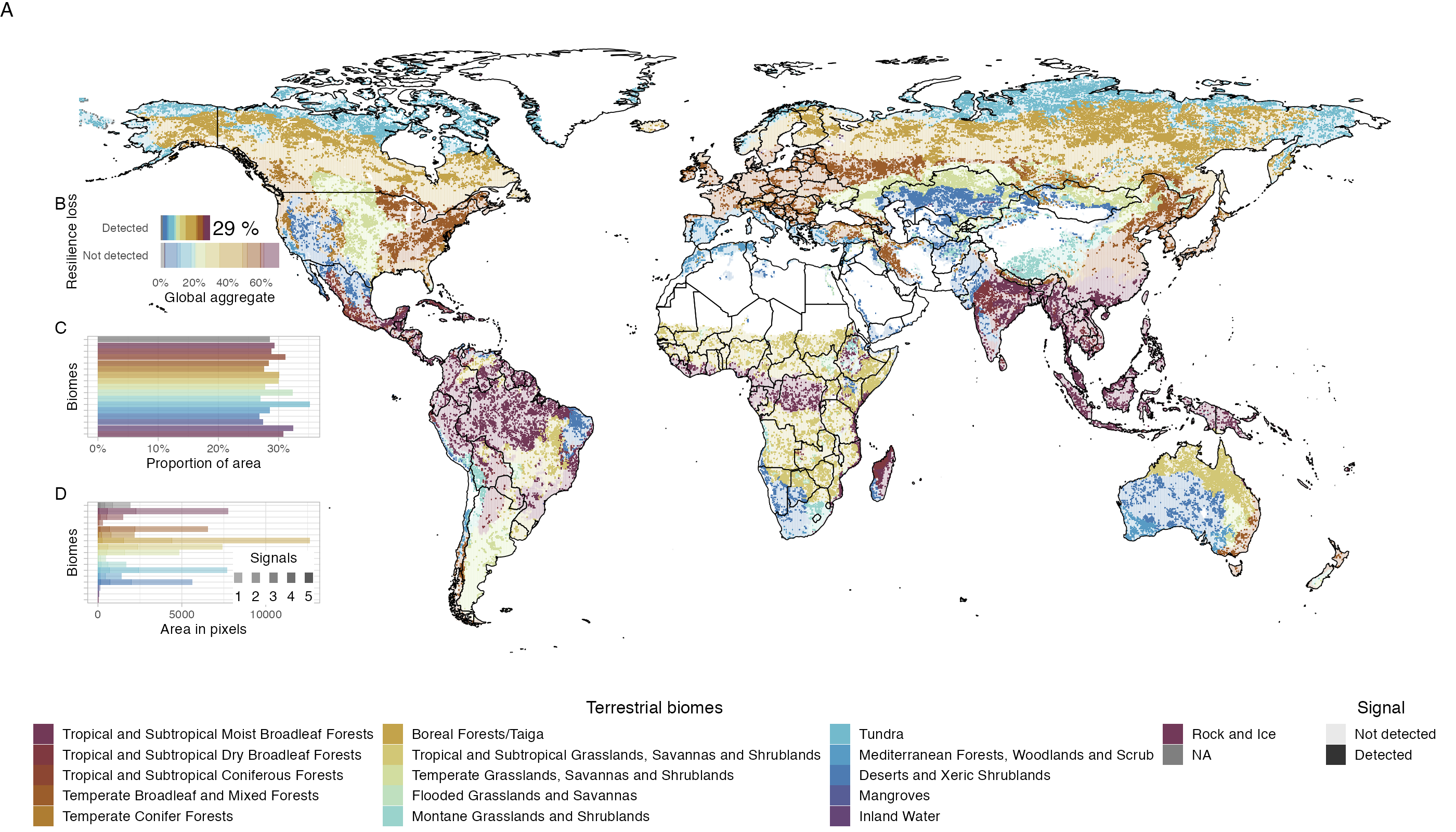
Figure 2: Resilience loss in terrestrial biomes Resilience loss for gross primary productivity is approximated as large differences in standard deviation, autocorrelation at lag-1, skewness, kurtosis or fractal dimension. Differences are considered a symptom of resilience loss if they are above the 95% or below 5% percentiles of the distribution. A) shows where are biomes showing symptoms of resilience loss, B) shows the global aggregate, C) shows aggregated proportion of area per biome, while D) shows area in 0.25 degree pixels accounting for the number of signals per pixel. A similar figure for terrestrial ecosystem respiration is available in Fig S1. Fig S2 provides maps for each resilience indicator on the gross primary productivity data, and Fig S3 on terrestrial ecosystem respiration.

The generic resilience indicators do not necessarily align with critical slowing down or speeding up theories. Fig 1 illustrates the analysis for one pixel where all indicators show signals of resilience loss. The time series is first pre-processed to remove confounding factors such as seasonality or long term oscillations, log-transformed to reduce the influence of outliers or shock events, and centered to zero mean and unit variance (Methods). All time series were first-differenced and passed a root test that guarantees stationarity; in other words, if a signal is detected it is not the product of residual long-term trends or seasonal variation on the data. The generic indicators are then calculated by using a rolling window with length equivalent to 50% of the data. To detect changes in trends of the indicators we used three approaches. First, $\Delta$ captures the difference between the minimum and maximum values of the indicator over time. By itself $\Delta$ is not very informative unless one has its distribution for the entire planet to compare against. In the pixel described in Fig 1 the observed $\Delta$ is indeed on the tail of the distribution for all indicators. Second, a linear regression was fitted to each indicator to test whether the slopes were different from zero, but it tends to treat sharp increases or decreases of the resilience indicators as outliers. Hence, the third approach was a segmented regression, enabling the detection of a point in time where there is a significant change on the slope of two linear regressions. The summary of the analysis for all pixels across all datasets shows that only in few cases autocorrelation and variance increase or decrease in tandem, the signatures of critical slowing down or speeding up. In contrast, large values of $\Delta$, interpreted here as symptoms of resilience loss, are detected in several different arrangments, most commonly in the agreement between kurtosis and skewness.

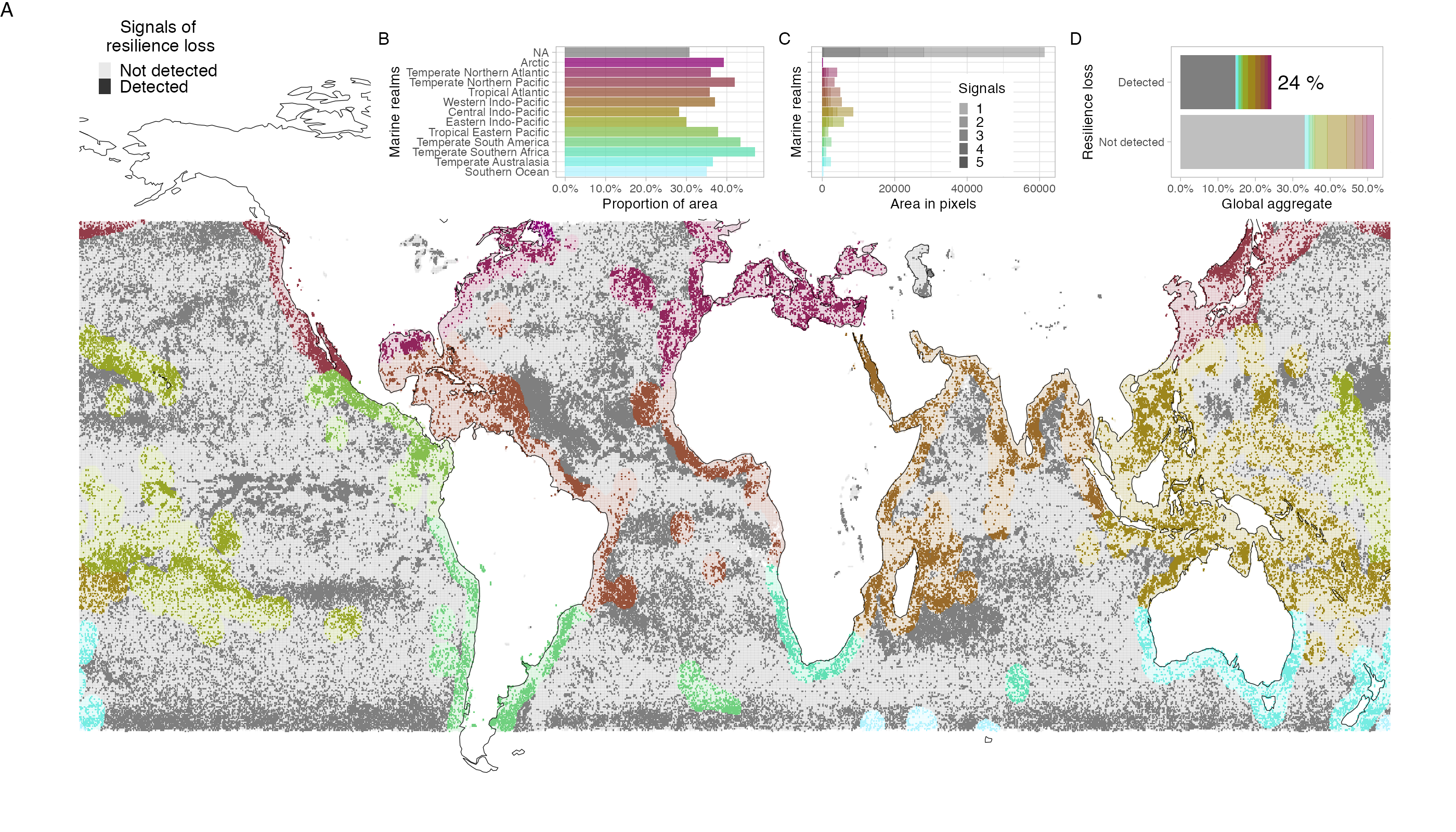
Figure 3: Resilience loss in marine realms Detection of resilience loss using chlorophyll-A as proxy of primary productivity (A). B) shows the global aggregate of resilience loss, C) shows aggregated proportion of area per marine realm, while D) shows area in 0.25 degree pixels accounting for the number of signals per pixel. Maps for each resilience indicator are provided in Fig S4.

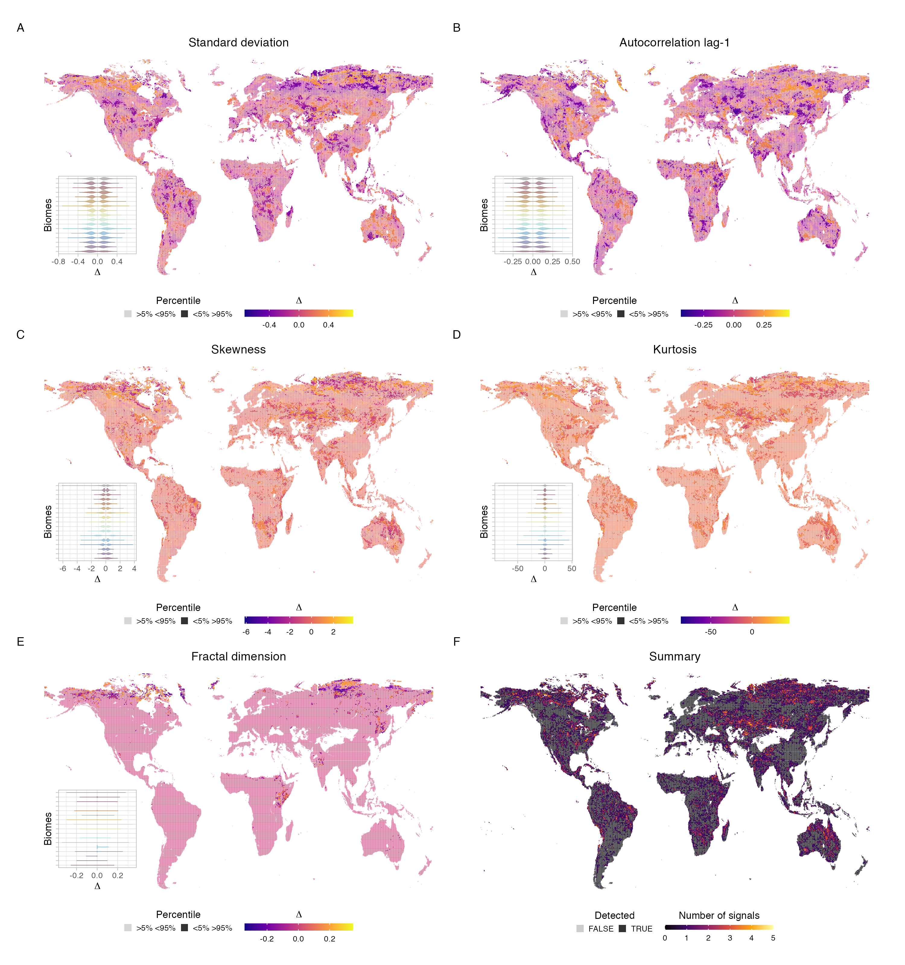
Figure S2: Resilience indicators in gross primary productivity Maps of the $\Delta$ outliers per biome are shown for standard deviation (A), autocorrelation at lag-1 (B), skewness (C), kurtosis (D), and fractal dimension (E). Insets show the distribution of $\Delta$ for each biome following the same colouring scheme of fig 2. (F) is the summary with the aggregated number of signals.

Ecosystems world-wide are showing symptoms of resilience loss. The absolute difference in resilience indicators ($\Delta$) emphasizes jumps in the time series and enables comparison with normal variation adjusted to each biome type. Arctic ecosystems such as boreal forests, taiga and tundra show the strongest signals of resilience loss globally (Fig 2, S1). However, the extremes of the distributions (5% and 95% percentiles) of each resilience proxy reveal that all ecosystems are losing resilience, for some of them up to 30% of their global area using the gross primary productivity or terrestrial ecosystem respiration data sets (Fig S2, S3). Despite data incompleteness for marine ecosystems at high latitudes, some signals of resilience loss are detected in Arctic marine systems and the Southern Ocean (Fig 3, S4). The Easter Indo-Pacific and Tropical Eastern Pacific Oceans are the marine realms with larger areas showing symptoms of resilience loss (Fig 3). The high oceans (gray area in Fig 3), however, show by far the larger areas affected with hot spots outside the Caribbean basin in the Tropical Atlantic, the Tropical Pacific and southeast Madagascar.

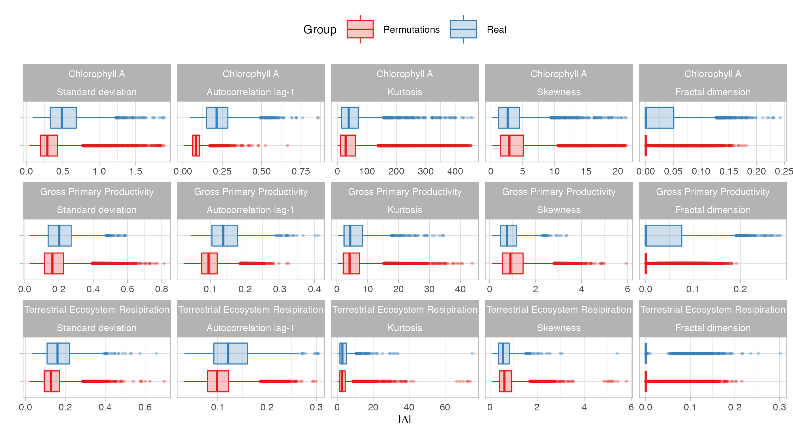
Figure 4: Permutations tests over time A sample of 500 pixels where resilience loss was detected by at least three indicators is compared against 5000 permutations of the same time series (10 permutations each). A Wilcoxon two sided test confirms differences in mean between the real and permuted time series (p << 0.05 for all comparisons).

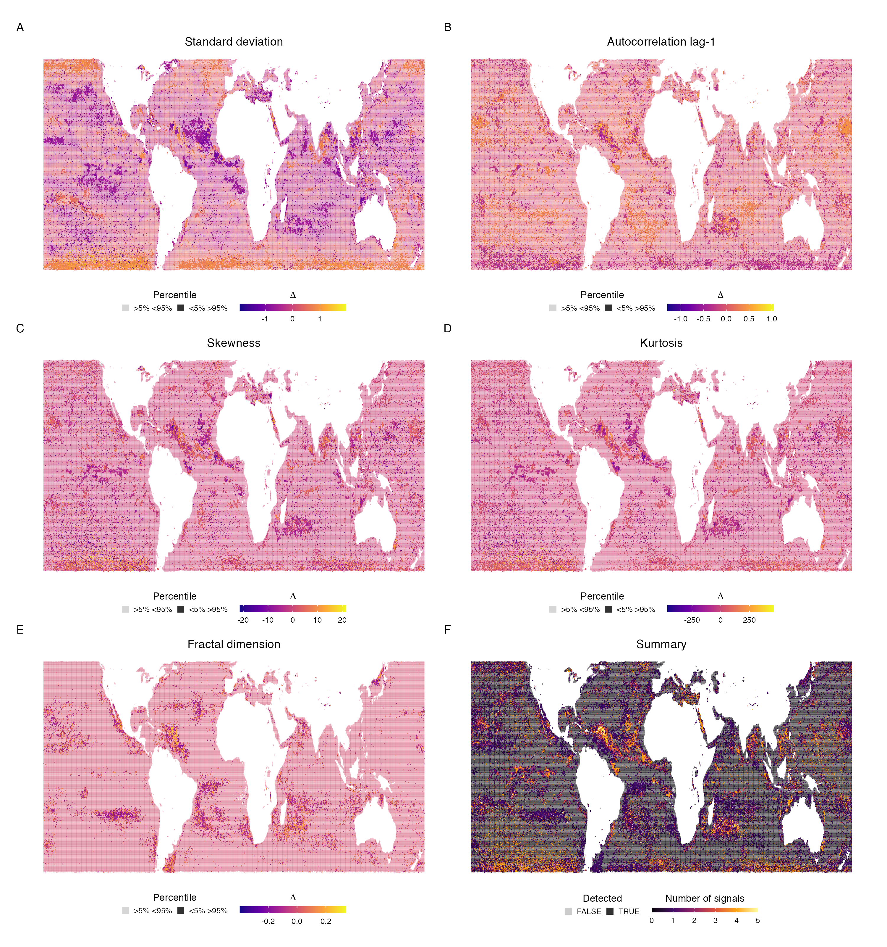
Figure S4: Resilience indicators in chlorophyll A Maps of the $\Delta$ outliers per biome are shown for standard deviation (A), autocorrelation at lag-1 (B), skewness (C), kurtosis (D), and fractal dimension (E). Insets show the distribution of $\Delta$ for each biome following the same colouring scheme of fig 3. (F) is the summary with the aggregated number of signals.

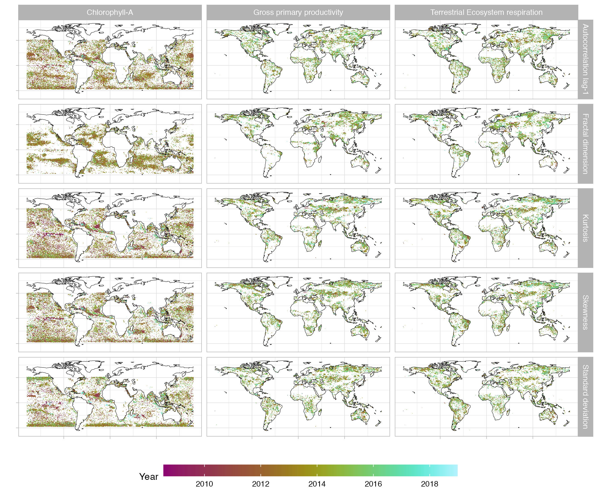
Figure S5: Spatial and temporal coherence Break points of the segmented regressions are show as maps for each dataset. The clustering in time and space of the dynamic indicators of resilience supports the idea that some areas are under similar pressures and can shift in tandem.

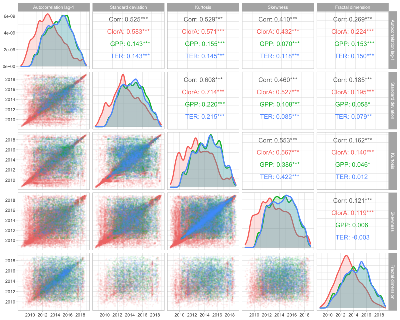
Figure S7: Temporal correlations Correlations in time of resilience indicators across datasets: gross primary productivity (GPP), terrestrial ecosystem respiration (TER), and chlorophyll A (ClorA)

Symptoms of resilience loss are coherent in space and time. Although the analysis was done independently for each time series and variable, spatial aggregation and coincidence of break points in time suggest that the signals are not artifacts of the data used (Fig S5, S6 , S7). On the contrary, it supports the idea that there are edges in the three-dimensional space (longitude, latitude and time) that enclose volumes whose dynamics can shift in tandem (30). Resilience indicators are remarkably consistent across metrics for marine systems both in space (Fig S4) and time (Fig S7). There is high agreement between kurtosis and skewness across all data sets (Figs S2, S3, S4); they can signal the possible shifting of basin of attraction or dynamic transients (1,10).

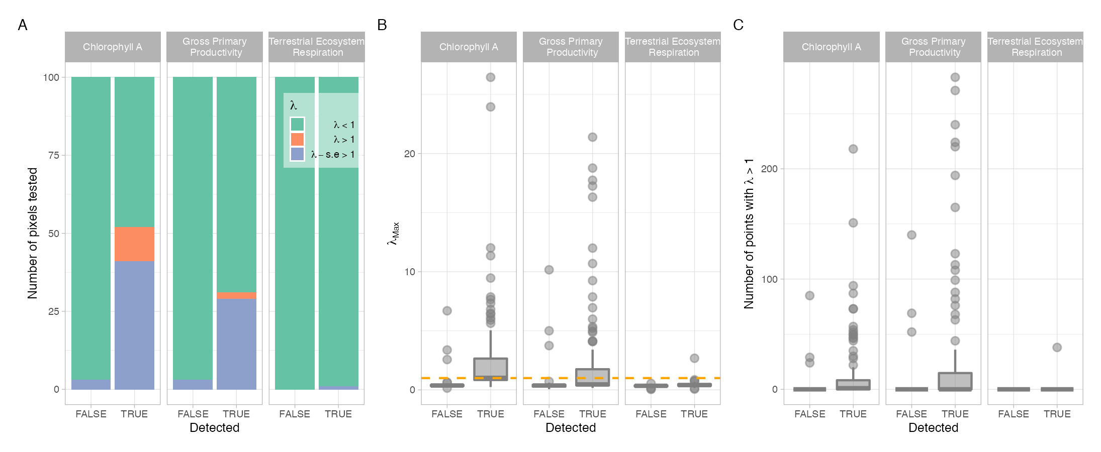
Figure 5: Model-based indicators A sample of 100 pixels where resilience loss was detected by at least three indicators is compared against 100 pixels where no signals were detected. The leading eigenvalue of the system is approximated with a dynamic linear autoregressive model

An alternative interpretation for coherence of signals is spatial and temporal autocorrelation, or that they are merely responses to shocks on environmental variables. Potential issues of temporal autocorrelation were dealt with by processing the data to the point that the remaining time series were stationary (32). Issues of spatial autocorrelation are dealt with (below) by fitting explanatory models and subsampling in space, while introducing fixed effects for geography related variables (biome, latitude, longitude). To further test the robustness of the signals, a subsample of time series of detected places (N = 500) were compared against the same time series but with the order of observations changed (10 permutations per time series, 5000 permutations). When the ordering of observations is lost, the signal of resilience loss disappears, meaning it has e.g. a significantly lower autocorrelation and standard deviation on the absolute value scale (Fig 4). A Wilcoxon two-sided test, comparing the distributions of permutations agains observed data, suggests that the means are indeed different (p << 0.05 for all comparisons). Thus, the results are not merely noise induced by outliers (e.g. shocks) because the same time series with the same outliers but different ordering does not show the early warnings to the same extent as the observed data. On the contrary, for some statistics like autocorrelation and standard deviation, their delta values go back to what is expected to be normal (the global median).

An additional robustness test is comparing the generic indicators against model-based early warnings. The latter are autoregressive dynamic linear models that enable fitting coefficients that change over time, in particular the approximation of the leading eigenvalue of the system $\lambda$ (26–28). For each dataset a sample of a hundred pixels was randomly drawn for detected places with at least three different resilience indicators, and compared against places that showed no early warning (Fig 5). Model-based indicators showed resilience loss for at least half of the sample of chlorophyll A and a third of the sample of gross primary productivity. For places where $\lambda<0$ the distribution still shows a displacement towards one when compared to places with no signals. For terrestrial ecosystem respiration however, model-based early warnings do not support the patterns found by the generic indicators.

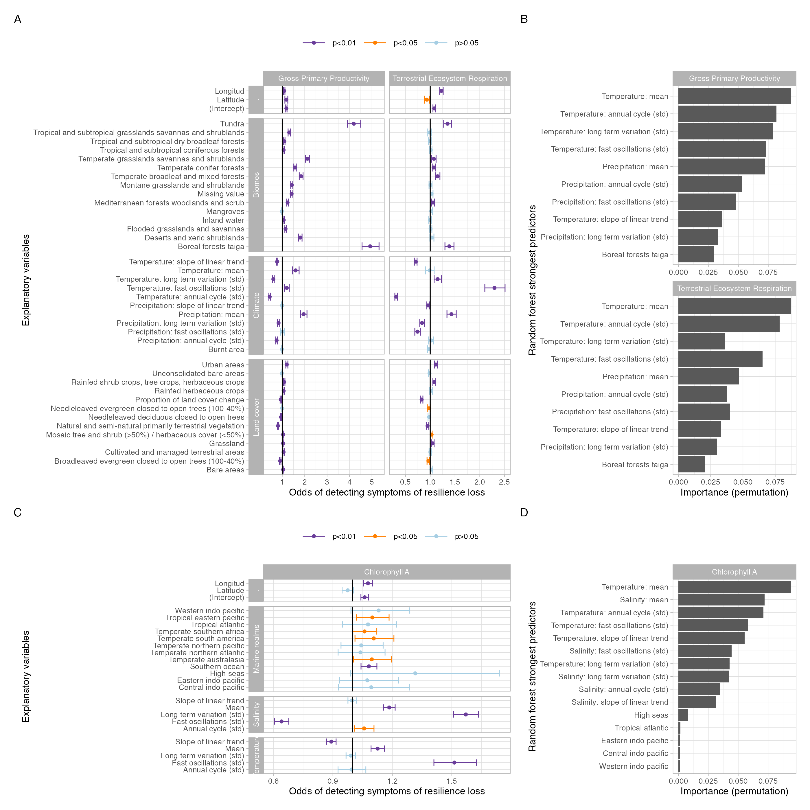
Figure 6: Predictors of resilience loss Logistic regressions to predict signals of resilience loss in gross primary productivity, terrestrial ecosystem respiration (A), and chlorophyll A (C). The strongest predictors of the random forest for terrestrial systems (B) and marine realms (D) were calculated with a permutation method. All random forest fitted 1000 trees. The best model for gross primary productivity targeted node size 10 and 12 variables to split at each node (N = 31122, OOB error 0.13), 20 node size and 9 variables for terrestrial ecosystem respiration (N = 29546, OOB error 0.14), and 20 node size and 9 variables for chlorophyll A (N = 54298, OOB error 0.16).

If resilience is approximated as the size of the basin of attraction, critical slowing down is sensible to reductions in depth while critical speeding up is sensible to reductions in width. However, these theories when applied to ecological problems are typically approached as low dimensional models with perhaps one controlling factor, one driver. Recent experimental evidence suggests that when ecosystems are subject to multiple drivers, early warning indicators can fail or provide contradictory signals (33). Lack of consistency between signals suggests that there is no one preferred theory at place. But instead, multiple drivers are interacting in pushing ecosystems outside their realm of stability, some of them through increasing stochasticity while others through slow forcing.

To test that hypothesis, I used logistic regressions and random forests to investigate what is driving the detection of early warnings. Detection by at least two proxies of resilience loss was used as a response variable. Explanatory variables for terrestrial ecosystems included time series of temperature, precipitation, burned area, and land cover. For marine systems, the explanatory variables were restricted to sea surface temperature and sea surface salinity. Variables with long and frequent time series (temperature, salinity and precipitation) were filtered with a Fourier transform to test whether the signals are predicted by long term variation, annual cycles, fast oscillations, or the linear (slow) trends. All regressions used a stratified sampling design, balanced on detection, and with fixed effects per biomes or marine realm respectively (See Method). The subsampling is necessary to control for two sources of bias. First, it breaks biases induced by spatial autocorrelation and the potential inflation of effects or small standard errors (32). Second, it reduces bias by a relatively larger amount of pixels were resilience loss is not detected, or by biomes that naturally have larger areas.

The strongest predictors of resilience loss are indeed a combination of slow forcing and stochasticity in environmental variables such as temperature, precipitation or sea surface salinity. For terrestrial biomes, mean temperature, mean precipitation and variability in fast oscillations and annual cycles are the strongest predictors, while marine realms are predicted by mean temperature, mean salinity and their variability at different time scales (Fig 6). The logistic regression facilitates a relatively straightforward interpretation (34). Once geography and biome type has been controlled for, the reminder coefficients indicate what increases the odds of detecting resilience loss. However, this linear approach suffers from correlations in the predictors, namely the different time scales at which the hypothesis needs to be tested, whether it is slow forcing or stochasticity at different time scales what drives the signals. In fact, the predicting accuracy for the logistic regression is poor (area under the receiver operating characteristic curve ROC 0.71, 0.65 and 0.59 for gross primary productivity, terrestrial ecosystem respiration and chlorophyll A respectively). The random forest approach leads to higher predictive power (ROC 0.893, 0.874, 0.827 respectively). It is robust to potential correlations and required less pre-processing for feature engineering but is less amenable to interpretation (34). It reveals which variables improve predictions but not necessarily in which direction they are affecting resilience loss. The results of both approaches confirm the hypothesis that resilience loss is driven by a combination of slow forcing and stochasticity on potential drivers.

Discussion

Resilience is the ability of any system to deal with change while keeping its structure and functions, thus its identity (11,12). The dynamic indicators used here approximate resilience as recovery time (1,22), and for the fractal dimension a collection of behaviors available to deal with disturbance (23). These metrics, however, do not directly inform about other dimensions of resilience such as the size of the basin of attraction, the amount of disturbance that the system can stand, the mean return time, the distance to tipping points and thresholds, or adaptive and transformative capacities (12,14). The indicators here used can be seen as symptoms of instabilities being developed on the time series of primary productivity for global ecosystems over the past two decades. The symptoms do not imply imminent regime shifts, they help identify places where their probability is increasing given the limitations of the data. The data is relatively short to account for critical transitions in the biosphere, yet it is one of the best observational records to approximate resilience globally. These symptoms are necessary but not sufficient evidence of unfolding regime shifts. Yet, the analysis here presented enables the identification of areas vulnerable to regime shifts at a scale relevant to decision makers.

Globally 29% of terrestrial biomes and 24% of marine realms show signals of resilience loss in at least one of the indicators used (Fig. 2, 3, S1). The overall patterns here reported agree with recent reports documenting ecosystems’ degradation worldwide. Forests are becoming more vulnerable to droughts, and the combined effects with increasing fire frequency are exposing them to major diebacks expected by mid-century (35). Temperature thresholds for terrestrial primary productivity have been identified (36,37) where carbon uptake is potentially degraded (sink to source transition). Less than 10% of the terrestrial biosphere has already crossed the threshold, and under business-as-usual scenarios, half of the biosphere is expected to cross these thresholds by the end of the century, with the most affected areas being Canadian and Russian boreal taigas as well as the Amazon and South East Asia rainforests (36). These are biomes where the strongest signals of resilience loss were detected with a right shift on the distribution of $\Delta$. Other studies quantifying terrestrial ecosystems’ resilience with NDVI data also show strong signals from tundra and boreal forests (38). A recent quantification of aridity thresholds shows that up to 28.6% of current dryland area can cross these thresholds by 2100 in the most drastic climate scenarios (39). The results here presented confirm early warning signals of resilience loss in drylands as well, particularly with the fractal dimension, skewness and kurtosis (Fig. S2, S3).

The marine patterns presented here also align with previous studies. Deepening of the ocean’s mixed layer can decrease light conditions near the surface, decreasing nutrient exchange in the water column and consequently primary productivity (40). The area outside the Caribbean basin reported here coincides with an area where salinity has contributed to ocean stratification (40). Upwelling systems are also hotspots where resilience loss is identified. Upwelling strength is expected to change with climate change, with strengthening already reported in the California and Benguela currents, while weakening in the Iberian-Canary system (41). Upwelling weakening can limit nutrients in marine food webs, while strengthening can over enrich nutrients and facilitate the onset of oxygen minimum zones (7). This study provides an additional line of support that these systems are being destabilized.

The results are limited by the temporal and spatial scale of the available data. If the grain of the data is not frequent enough to match fast dynamics, long enough to capture change in slow processes (1,10,16), or the spatial resolution is too coarse, local transitions in space and time can be missed. This is the case with hypoxic areas, where large oxygen minimum zones are identified, but not the diverse range of smaller local cases that have been previously reported (7). Only regime shifts that are drastic enough to change primary productivity as observed from remote sensing products can be identified. Regime shifts that impact specific populations or community assemblies without changing primary productivity are missed. Such is the case of coral transitions in the Great Barrier Reef where ~50% of the reef community collapsed following the heatwave events of 2016-17 (42).

Because of these limitations, the results likely are an underestimation. The estimates are also conservative, with an arbitrary 5% and 95% quantile of the $\Delta$ distribution as detection threshold. A lower cutoff would enlarge the areas where resilience loss is detected, but also increase the risk of false positives. A similar study using NDVI data estimated up to ~65% of terrestrial ecosystems show early warning of critical transitions, with strong bias towards boreal forest and taiga (38). The estimates presented here complement previous efforts (29,38) in taking into consideration fixed effects by biome and a pre-processing technique that removes seasonality and long-term variations that can lead to errors, or bias towards high variable environments (higher latitudes).

Another limitation of this study is the lack of ground truthing. The results provide a spatial prediction of where ecosystems might be losing their resilience. But since critical transitions have not happened yet in many of these places, it is not possible to contrast the models presented here with their real predicting power. Current databases that track such transitions are biased to studies and observations on the global north and coastal ecosystems (7,9), their coverage is not yet sufficient to be used as ground truth across all ecosystems and biomes. Nevertheless, the robustness of the signals detected were tested against null permutation models and model-based early warnings. The first test showed the signals are not an artifact of the data, potential temporal autocorrelation was dealt with stringent data pre-processing and randomizing the ordering of observations. The second test supported our findings for chlorophyll A and gross primary productivity, but failed in supporting the findings of terrestrial ecosystem respiration.

Model-based approaches such as autoregressive time varying models can help interpreting the results and robustness of generic indicators (26–28). In this study, these methods gave stronger confidence to the results from gross primary productivity and less support to terrestrial ecosystem respiration derived signals, although both results qualitatively point to the same patterns. The combination of methods thus helped distinguish what are optimal observables of resilience loss, an open question and possibly a fruitful avenue for future research (10). Unfortunately, model-based methods are computationally expensive and do not scale up to the data requirements of remote sensing products, on the order of $10^{5}$ to $10^{7}$ spatial pixels (depending on spatial resolution) times time series length. Generic indicators are still useful in narrowing down the scope at which computationally expensive methods become practical.

Computing the probability density function of $\Delta$ helps interpreting signals of resilience loss. Previous work using generic indicators typically have ground truth in the form of modeling simulations with some noise or actual experiments. Because the ground truth is known, there was not concern whether the magnitude of the increase (decrease) in early warnings was big enough to actually be considered a warning. Here we do not have ground truth like experiments, but we can compute the distribution of each indicator for the entire planet enabling the comparison of what constitutes a big jump on an indicator as opposed to its normal expected variability for each biome. The magnitude depends on the indicator and data pre-processing choices, but the position of the pixel in the distribution is relatively unaffected. Thus, $\Delta$ is less sensitive to pre-processing choices. While in theory increases or decreases on a particular statistic can be interpreted as resilience loss (an apparent contradiction), the distribution of $\Delta$ helps interpreting whether an increase or decrease is towards the tails of the distribution (resilience loss) as opposed to an increase or decrease towards the center of the distribution (a resilience gain). The fractal dimension here introduced is unambiguous and do not depend on scale, for time series it is bounded between 1 and 2 and higher values are always more resilient (23,43). Future studies can use these two facts to track ecological recovery.

Despite its limitations, this first-order approximation to resilience loss can help outline priority areas for management. Russia, Canada, the US, and Australia are countries with the largest areas of resilience loss identified, yet by proportion of territory, small island states top the ranking. When accounting for the diversity of ecosystems showing signs of resilience loss, megadiverse countries like Brazil, India, Mexico, Indonesia, Australia, or Colombia are on the top 10 (Fig 7). Australia has recently been reported as a hotspot for ecological collapses for both marine and terrestrial ecosystems (44). The spatial resolution of the maps here presented enable countries, regions, and even municipalities to update land use planning and take the vulnerability of their ecosystems into consideration. Companies for example, can take such risk into account when deciding on relocation, resource outsourcing, or investments. Countries and municipalities can balance the trade-off between maximizing a particular ecosystem service (e.g. a monoculture) in favour of multifunctional landscapes that include other values such as recreation, spiritual values or conservation. No matter the scale, we all have a role to play in caring for ecosystems resilience and maintaining their ability to provide the ecosystem services we all depend on.

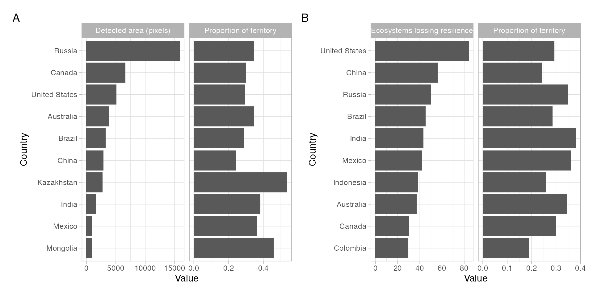
Figure 7: Most affected countries Top 10 countries by aggregated area in 0.25 degree pixels showing symptoms of resilience loss and as proportion of their territory (A). Countries ranked in (B) by the number of unique ecosystems showing symptoms of resilience loss and their proportion of territory impacted.

Future global resilience assessments could benefit from other data streams, particularly other anthropogenic drivers overlooked here. Additional data would however require long time series coverage and high spatial resolution. The accuracy of the predictive models presented here can be improved by using non-linear approaches such as deep neural networks or other machine learning techniques (45). However, these approaches have limited interpretability and often require manually annotated datasets to measure performance. Qualitative efforts such as the Global Ocean Oxygen Network (7) or the Regime Shifts Database (9) can provide the annotated examples to train such models. A spatially explicit map of resilience loss can also help quantify the risk of cascading effects in ecosystems previously identified (46). As new Earth observations become available, these global maps can be updated and track how ecosystems resilience is evolving, where are they recovering and where they are becoming more vulnerable. This paper showcases the first steps toward an ecological resilience observatory.

Methods

Data: Gross primary productivity, terrestrial ecosystem respiration (both in $gCm^{-2}d^{-1}$), and chlorophyll-a concentration ($mgm^{-3}$) were used as proxies of primary productivity of terrestrial and marine ecosystems respectively (47–49). Although these data sets are freely available through the FLUXCOM initiative (http://www.fluxcom.org) or the European Space Agency Climate Change initiative (https://climate.esa.int/), the versions of the data used here were harmonized by the Earth System Data Lab to weekly observations at 0.25 degree grid resolution, and stored as Zarr data cubes to facilitate out of memory computations (31). Gross primary productivity and terrestrial ecosystem respiration time series span the period 2001-2018 resulting in 210 771 terrestrial pixels with 817 time observations each, while chlorophyll A span the period 1998-2018 resulting in 418 776 time series with 966 observations each. The Nature Conservancy classification of terrestrial biomes and ecosystems was used (16 biomes, 812 ecosystems) based on (50), while marine realms (N=12) followed (51) classification.

Pre-processing: The Earth System Data Lab is hosted by the Max Planck Institute of Biogeochemestry and Brockmann Consult GmbH with the support of the European Space Agency. Their computing services were used to pre-process the data in their Julia environment. For each of the resulting time series, missing data was inputted with the mean seasonal cycle. A fast Fourier transform was used to filter the time series and remove the trend, annual cycle, and long-term variability. The remaining fast oscillations were log-transformed and normalized to zero mean and unit variance. The cleaned data was exported and further statistical analysis performed in R. A unit root test showed that a few time series were not stationary after the pre-processing steps described. Thus all time series were first-differenced to remove any remaining seasonality.

Proxies of resilience: At this point all time series are expected to have zero mean and unit variance. Resilience loss is here detected by measuring critical slowing down or speeding up in terms of sharp increase (decrease) of variance measured as standard deviation, autocorrelation coefficient at lag-1; or proxies of flickering such as skewness, and kurtosis. Fractal dimensions were calculated using the madogram method (43). All these statistics were calculated in rolling windows half of the size of the time series available. $\Delta$ is the difference between maximum and minimum values of the resilience indicators considering time ordering (thus allowing negative values). For standard deviation and autocorrelation at lag-1, a positive $\Delta$ can indicate critical slowing down or speeding up if negative. The value of $\Delta$ however is not informative by itself. The magnitude depends on the pre-processing choices. Other researchers prefer a Gaussian filter, or kernel based methods to pre-process time series. These methods, however, require arbitrary choices that can optimize for detection of certain biomes while under-estimating for others. Because the data analyzed spanned about two decades, care should be taken to avoid bias on the resilience indicator by seasonal variability, annual cycles or multidecadal oscillations. For these reasons the Fourier transform was an ideal filter for this study, returning zero mean and unit variance fast oscillations regardless of whether the time series comes from a strong seasonal biome (e.g. boreal forest) or weak seasonality (e.g. tropical ones). The value of $\Delta$ varies, however, with window size, the smaller the rolling window, the larger $\Delta$ becomes. What matters, however, is not the absolute value of $\Delta$ but its position relative to the distribution for the planet, and in particular, relative to the biome described (due to the seasonality differences). $\Delta$ has a bimodal distribution (because zero differences are very unlikely), and outliers with respect to each biome distribution were reported as places showing symptoms of resilience loss. Outliers are here defined as places where $\Delta$ is unusually extreme, either above the 95% or below the 5% quantiles of $\Delta$ distribution.

To check for the spatial and temporal coherence across time series, a segmented regression (52) was used to identify the breaking point at which the early warning is detected. The segmented regression departed from a linear fit of the resilience proxy against time, the median of the indicator was used as starting value, and only one break point was calculated by default. A Davis tested for the significant difference in slopes before and after the breaking point. Since the time series are normalized, the expectation is no difference in variance and hence no detection of breaking points. If there is a breaking point and the difference is significant and large, one can expect the signal to be a warning of resilience loss, specially in the case where other neighboring areas show similar signals in space and time. The statistical detection treats each time series independently, but spatial and temporal coherence of the signal offers supporting evidence for true detection in the absence of annotated data or ground truth. An additional line of support can be explored by training models that exploit information about potential causes of abrupt changes in ecosystems to predict the detection (or lack) of resilience loss.

Regressions: To further test the robustness of the results and explore what is driving resilience loss, a logistic regression and a random forest were fitted to classify pixels where at least two metrics suggested loss of resilience. Explanatory variables included air temperature at 2m (https://cds.climate.copernicus.eu/cdsapp#!/dataset/ecv-for-climate-changee), sea surface temperature (53) (https://climate.esa.int/en/projects/sea-surface-temperature), precipitation (https://gpm.nasa.gov/data), sea surface salinity (https://climate.esa.int/en/projects/ocean-colour), burned area (http://www.globalfiredata.org), and land cover change (https://cds.climate.copernicus.eu/cdsapp#!/dataset/satellite-land-cover). For all variables, except land cover, the available data match the temporal resolution of the data used as proxy of primary productivity, but not necessarily time span. Thus, a Fourier transform was used to pre-process the data and separate the linear trend, seasonal cycle, annual cycle and fast oscillations. For temperature, precipitation and salinity, their mean value, slope of the linear trend and the standard deviation of the seasonal cycle, annual cycle and fast oscillations were used as regressors. This is with the intention of testing whether resilience loss is driven by variability at different time scales or changes in slow processes. Land cover data has a higher spatial resolution (300m) but lower temporal resolution (year). Proportion of change per land cover class between 1994 and 2018 were calculated and aggregated at 0.25 degree grid. Burnt area is the aggregated area burned in hectares during 2001-2018 per pixel.

For logistic regressions, the data was down sampled on the detection variable (at least two variables indicating resilience loss), after filtering out rock and ice biomes, log-transforming burnt area, performing a box-cox transformation on land cover change variables, and normalizing to zero mean and unit variance all numeric predictors. Random forest, being more tolerant to variables on their natural units, were fitted after filtering out rock and ice biomes and down sampling on detection. 75% of the data was used for training and tuning hyper parameters using 10-fold cross validation. All random forests were fitted with 1000 trees. Best models were assessed against the testing data (25%) and variable importance computed with permutation. The best model for gross primary productivity targeted node size 10 and 12 variables to split at each node (N = 31122, OOB error 0.13), 20 node size and 9 variables for terrestrial ecosystem respiration (N = 29546, OOB error 0.14), and 20 node size and 9 variables for chlorophyll A (N = 54298, OOB error 0.16).

Data availability: All data used in this study is publicly available through the Copernicus Climate Change and Atmosphere Monitoring Service, NASA, FLUXCOM initiative, or the Global fire emissions database. Links to each data set are provided when introduced under the section data or regressions.

Computer code: All code used in this analysis is available at https://github.com/juanrocha/ESDL.

References

re 1. Scheffer M, Bascompte J, Brock WA, Brovkin V, Carpenter SR, Dakos V, et al. Early-warning signals for critical transitions. Nature. 2009;461(7260):53–9.

pre 2. Folke C, Carpenter S, Walker B, Scheffer M, Elmqvist T, Gunderson L, et al. Regime shifts, resilience, and biodiversity in ecosystem management. Annu Rev Ecol Evol S. 2004 Dec;35(1):557–81.

pre 3. Hirota M, Holmgren M, Nes EH van, Scheffer M. Global resilience of tropical forest and savanna to critical transitions. Science. 2011 Oct;334(6053):232–5.

pre 4. Hughes TP, Barnes ML, Bellwood DR, Cinner JE, Cumming GS, Jackson JBC, et al. Coral reefs in the Anthropocene. Nature. 2017 May;546(7656):82–90.

pre 5. Ling SD, Scheibling RE, Rassweiler A, Johnson CR, Shears N, Connell SD, et al. Global regime shift dynamics of catastrophic sea urchin overgrazing. Philos Trans R Soc Lond, B, Biol Sci. 2015 Jan;370(1659):20130269–9.

pre 6. Turetsky MR, Benscoter B, Page S, Rein G, Werf GR van der, Watts A. Global vulnerability of peatlands to fire and carbon loss. Nature Geoscience. 2015 Jan;8(1):11–4.

pre 7. Breitburg D, Levin LA, Oschlies A, Grégoire M, Chavez FP, Conley DJ, et al. Declining oxygen in the global ocean and coastal waters. Science. 2018 Jan;359(6371):eaam7240.

pre 8. Díaz RJ, Rosenberg R. Spreading Dead Zones and Consequences for Marine Ecosystems. Science. 2008 Aug;321(5891):926–9.

pre 9. Biggs R, Peterson G, Rocha J. The Regime Shifts Database: a framework for analyzing regime shifts in social-ecological systems. Ecology and Society. 2018 Jul;23(3):art9.

pre 10. Dakos V, Carpenter SR, Nes EH van, Scheffer M. Resilience indicators: prospects and limitations for early warnings of regime shifts. Philos Trans R Soc Lond, B, Biol Sci. 2015 Jan;370(1659):20130263–3.

pre 11. Holling CS. Resilience and stability of ecological systems. Annual review of ecology and systematics. 1973;4:1–23.

pre 12. Folke C. Resilience (Republished). Ecology and Society. 2016;21(4):art44.

pre 13. Clark WC. Notes on Resilience Measures. 1975; Available from: http://pure.iiasa.ac.at/id/eprint/338/

pre 14. Krakovská H, Kühn C, Longo IP. Resilience of dynamical systems. ArXiv [Internet]. 2021 May; Available from: http://arxiv.org/abs/2105.10592v1

pre 15. Scheffer M. Critical Transitions in Nature and Society. Princeton University Press; 2009.

pre 16. Arani BMS, Carpenter SR, Lahti L, Nes EH van, Scheffer M. Exit time as a measure of ecological resilience. Science. 2021 Jun;372(6547).

pre 17. Strogatz SH. Nonlinear Dynamics and Chaos. Hachette UK; 2014. (With applications to physics, biology, chemistry, and engineering).

pre 18. Scheffer M, Carpenter SR, Lenton TM, Bascompte J, Brock W, Dakos V, et al. Anticipating Critical Transitions. Science. 2012 Oct;338(6105):344–8.

pre 19. Kéfi S, Guttal V, Brock WA, Carpenter SR, Ellison AM, Livina VN, et al. Early Warning Signals of Ecological Transitions: Methods for Spatial Patterns. PLoS ONE. 2014 Mar;9(3):e92097.

pre 20. Hastings A, Abbott KC, Cuddington K, Francis T, Gellner G, Lai Y-C, et al. Transient phenomena in ecology. Science. 2018 Sep;361(6406):eaat6412.

pre 21. Hastings A, Wysham DB. Regime shifts in ecological systems can occur with no warning. Ecol Lett. 2010 Apr;13(4):464–72.

pre 22. Titus M, Watson J. Critical speeding up as an early warning signal of stochastic regime shifts. Theor Ecol. 2020 Feb;280(1766):20131372.

pre 23. West G. Scale. Penguin; 2017. (The universal laws of life, growth, and death in organisms, cities, and in organisms, cities, economies, and companies).

pre 24. West BJ. Fractal physiology and the fractional calculus: a perspective. Front Physiol. 2010;1.

pre 25. Pavithran I, Sujith RI. Effect of rate of change of parameter on early warning signals for critical transitions. 2021 Jan;(1):013116. Available from: https://arxiv.org/abs/2101.11811v1

pre 26. Ives AR, Dakos V. Detecting dynamical changes in nonlinear time series using locally linear state-space models. Ecosphere [Internet]. 2012 Jun;3(6):art58. Available from: http://www.esajournals.org/doi/abs/10.1890/ES11-00347.1

pre 27. Taranu ZE, Carpenter SR, Frossard V, Jenny J-P, Thomas Z, Vermaire JC, et al. Can we detect ecosystem critical transitions and signals of changing resilience from paleo-ecological records? Ecosphere [Internet]. 2018 Oct;9(10). Available from: https://esajournals.onlinelibrary.wiley.com/doi/full/10.1002/ecs2.2438

pre 28. Carpenter SR, Brock WA, Cole JJ, Pace ML. A new approach for rapid detection of nearby thresholds in ecosystem time series. Oikos [Internet]. 2013 Oct;123(3):290–7. Available from: http://doi.wiley.com/10.1111/j.1600-0706.2013.00539.x

pre 29. Verbesselt J, Umlauf N, Hirota M, Holmgren M, Nes EH van, Herold M, et al. Remotely sensed resilience of tropical forests. Nature Climate Change. 2016 Sep;6(11):1028–31.

pre 30. Bathiany S, Hidding J, Scheffer M. Edge Detection Reveals Abrupt and Extreme Climate Events. J Climate. 2020 Jun;33(15):6399–421.

pre 31. Mahecha MD, Gans F, Brandt G, Christiansen R, Cornell SE, Fomferra N, et al. Earth system data cubes unravel global multivariate dynamics. Earth System Dynamics. 2020;11(1):201–34.

pre 32. Ives AR, Zhu L, Wang F, Zhu J, Morrow CJ, Radeloff VC. Statistical inference for trends in spatiotemporal data. Remote Sensing of Environment. 2021;266:112678.

pre 33. Dai L, Korolev KS, Gore J. Relation between stability and resilience determines the performance of early warning signals under different environmental drivers. P Natl Acad Sci Usa. 2015 Aug;112(32):10056–61.

pre 34. Kuhn M, Johnson K. Applied Predictive Modeling. Springer Science & Business Media; 2013.

pre 35. Williams AP, Allen CD, Macalady AK, Griffin D. Temperature as a potent driver of regional forest drought stress and tree mortality. Commun Biol. 2013;3.

pre 36. Duffy KA, Schwalm CR, Arcus VL, Koch GW, Liang LL, Schipper LA. How close are we to the temperature tipping point of the terrestrial biosphere? Science Advances. 2021 Jan;7(3):eaay1052.

pre 37. Johnston ASA, Meade A, Ardö J, Arriga N, Black A, Blanken PD, et al. Temperature thresholds of ecosystem respiration at a global scale. Nature Ecology & Evolution. 2021 Apr;5(4):487–94.

pre 38. Feng Y, Su H, Tang Z, Wang S, Zhao X, Zhang H, et al. Reduced resilience of terrestrial ecosystems locally is not reflected on a global scale. Commun Biol. 2021;2(88).

pre 39. Berdugo M, Delgado-Baquerizo M, Soliveres S, Hernández-Clemente R, Zhao Y, Gaitán JJ, et al. Global ecosystem thresholds driven by aridity. Science. 2020 Feb;367(6479):787–90.

pre 40. Sallée J-B, Pellichero V, Akhoudas C, Pauthenet E, Vignes L, Schmidtko S, et al. Summertime increases in upper-ocean stratification and mixed-layer depth. Nature. 2021 Mar;591(7851):592–8.

pre 41. Sydeman WJ, García-Reyes M, Schoeman DS, Rykaczewski RR, Thompson SA, Black BA, et al. Climate change and wind intensification in coastal upwelling ecosystems. Science. 2014 Jul;345(6192):77–80.

pre 42. Hughes TP, Kerry JT, Baird AH, Connolly SR, Dietzel A, Eakin CM, et al. Global warming transforms coral reef assemblages. Nature. 2018 Apr;556(7702):492–6.

pre 43. Gneiting T, Ševčíková H, Percival D. Estimators of fractal dimension: Assessing the roughness of time series and spatial data. 2012;27(2):247–77.

pre 44. Bergstrom DM, Wienecke BC, Hoff J van den, Hughes L, Lindenmayer DB, Ainsworth TD, et al. Combating ecosystem collapse from the tropics to the Antarctic. Glob Change Biol. 2021 May;27(9):1692–703.

pre 45. Reichstein M, Camps-Valls G, Stevens B, Jung M, Denzler J, Carvalhais N, et al. Deep learning and process understanding for data-driven Earth system science. Nature. 2019 Feb;566(7743):195–204.

pre 46. Rocha JC, Peterson G, Bodin O, Levin S. Cascading regime shifts within and across scales. Science. 2018 Dec;362(6421):1379–83.

pre 47. Jung M, Koirala S, Weber U, Ichii K, Gans F, Camps-Valls G, et al. The FLUXCOM ensemble of global land-atmosphere energy fluxes. Scientific Data. 2019 May;6(1):74.

pre 48. Tramontana G, Jung M, Schwalm CR, Ichii K, Camps-Valls G, R ’aduly B, et al. Predicting carbon dioxide and energy fluxes across global FLUXNET sites with regression algorithms. BIOGEOSCIENCES. 2016;13(14):4291–313.

pre 49. Sathyendranath S, Brewin RJW, Brockmann C, Brotas V, Calton B, Chuprin A, et al. An Ocean-Colour Time Series for Use in Climate Studies: The Experience of the Ocean-Colour Climate Change Initiative (OC-CCI). Sensors (Basel). 2019 Oct;19(19).

pre 50. Olson DM, Dinerstein E, Wikramanayake ED, Burgess ND, Powell GVN, Underwood EC, et al. Terrestrial Ecoregions of the World: A New Map of Life on Earth. BioScience. 2001;51(11):933.

pre 51. Spalding MD, Fox HE, Allen GR, Davidson N, Ferdaña ZA, Finlayson M, et al. Marine Ecoregions of the World: A Bioregionalization of Coastal and Shelf Areas. BioScience. 2007 Jul;57(7):573–83.

pre 52. Muggeo VMR. Estimating regression models with unknown break-points. Stat Med. 2003;22(19):3055–71.

pre 53. Merchant CJ, Embury O, Bulgin CE, Block T, Corlett GK, Fiedler E, et al. Satellite-based time-series of sea-surface temperature since 1981 for climate applications. Scientific Data. 2019 Oct;6(1):223.

p

Supplementary Material

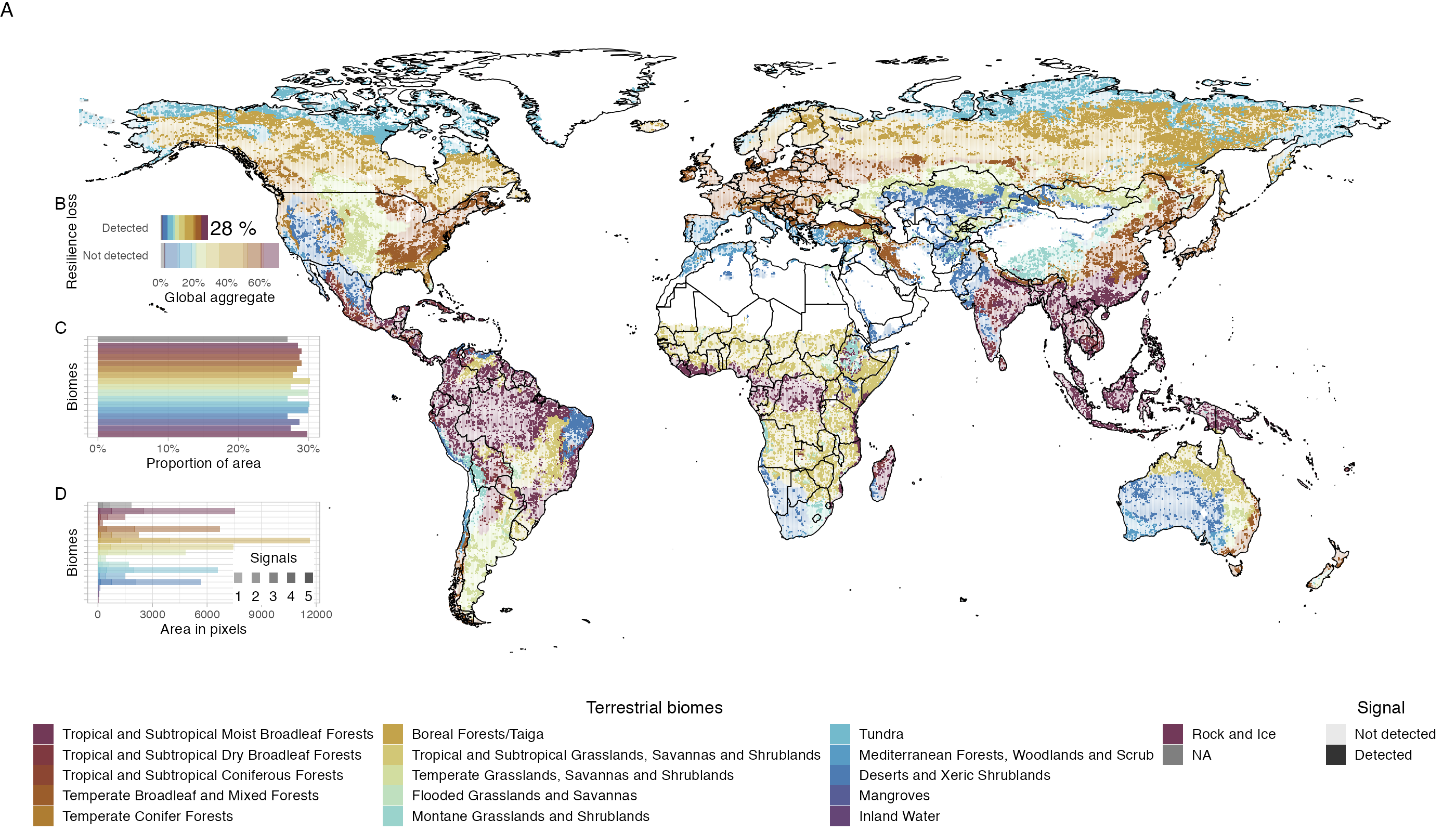
Figure S1: Terrestrial ecosystem respiration Detection of resilience loss in terrestrial biomes for terrestrial ecosystem respiration. A) shows where biomes are showing symptoms of resilience loss, B) shows the global aggregate, C) shows aggregated proportion of area per biome, while C) shows area in 0.25 degree pixels.

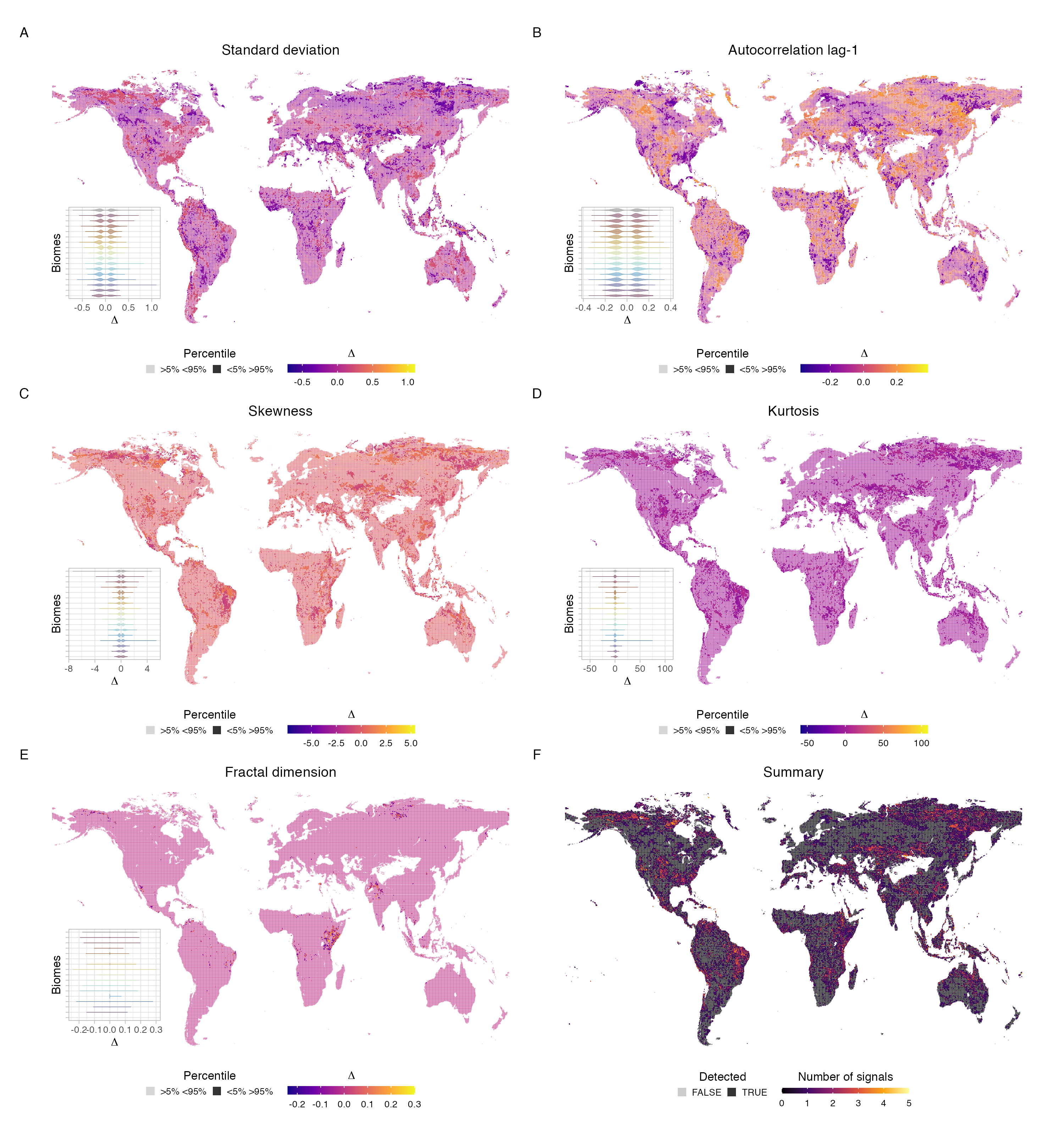
Figure S3: Resilience indicators in terrestrial ecosystem respiration Maps of the $\Delta$ outliers per biome are shown for standard deviation (A), autocorrelation at lag-1 (B), skewness (C), kurtosis (D), and fractal dimension (E). Insets show the distribution of $\Delta$ for each biome following the same colouring scheme of fig S1. (F) is the summary with the aggregated number of signals.

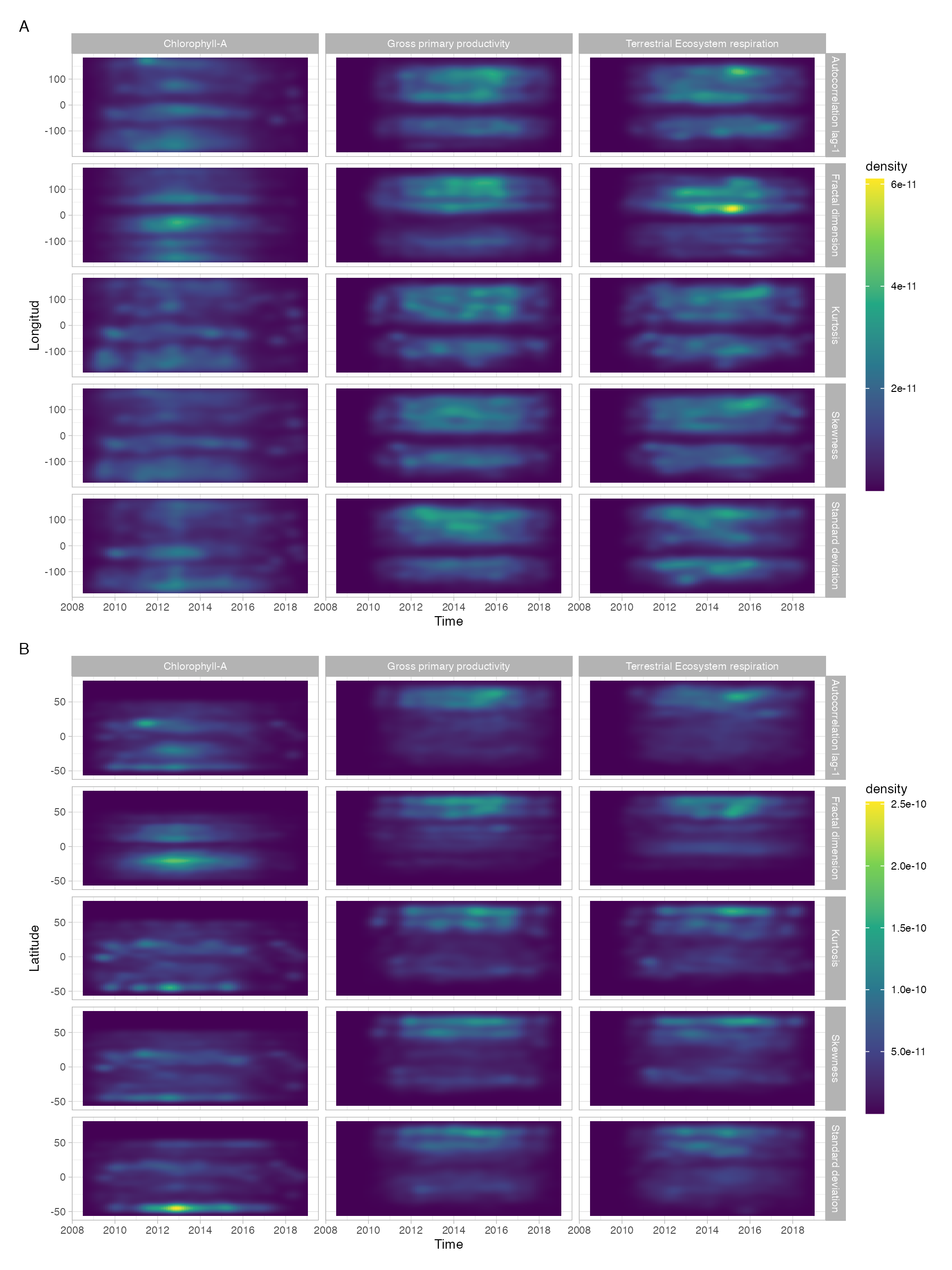
Figure S6: Temporal coherence of signals Probability density function of the location of break points in time and space for longitude (A) and latitude (B).