Funnel MPC for nonlinear systems with relative degree one

Abstract

We show that Funnel MPC, a novel Model Predictive Control (MPC) scheme, allows tracking of smooth reference signals with prescribed performance for nonlinear multi-input multi-output systems of relative degree one with stable internal dynamics. The optimal control problem solved in each iteration of Funnel MPC resembles the basic idea of penalty methods used in optimization. To this end, we present a new stage cost design to mimic the high-gain idea of (adaptive) funnel control. We rigorously show initial and recursive feasibility of Funnel MPC without imposing terminal conditions or other requirements like a sufficiently long prediction horizon.

Key words: model predictive control, funnel control, reference tracking, nonlinear systems, initial feasibility, recursive feasibility

AMS subject classifications: 34H05, 49J30, 93B45, 93C10

1 Introduction

Model Predictive Control (MPC) is a well-established control technique which relies on the iterative solution of Optimal Control Problems (OCPs), see the textbooks [11, 24]. Thanks to its applicability to multi-input multi-output nonlinear systems and its ability to take control and state constraints directly into account, it is nowadays widely used and has seen various applications; see e.g. [23].

A key property for applying MPC is recursive feasibility, meaning that solvability of the OCP at a particular time instant automatically implies solvability of the OCP at the successor time instant. Often, suitably designed terminal conditions (costs and constraints) are incorporated in the iteratively solved OCP to ensure recursive feasibility, see e.g. [24] and the references therein. However, such (artificially introduced) terminal conditions complicate the task of finding an initially-feasible solution by imposing additional state constraints. As a consequence, the domain of the MPC feedback controller might become significantly smaller. An alternative approach, which is based on so-called cost controllability [7], is using a sufficiently-long prediction horizon, see e.g. [5] and the references therein or [9] for an extension to continuous-time systems. It is worth to be noted that both techniques become significantly more involved in the presence of time-varying state (or output) constraints.

To overcome the outlined restrictions for a large system class, Funnel MPC (FMPC) was proposed in [3], which allows for reference tracking such that the tracking error evolves in a pre-specified, potentially time-varying performance funnel. To this end, output constraints were incorporated in the OCP. Then, both initial and recursive feasibility were rigorously shown by using properties of the system class in consideration – without imposing additional terminal conditions and independent of the length of the prediction horizon. Moreover, the range of applied control values and the overall performance were further improved by using a “funnel-like” stage cost, which penalises the tracking error and becomes infinite when approaching the funnel boundary.

In the present paper, we show that such funnel-inspired stage costs (slightly modified compared to its predecessor proposed in [3]) automatically ensure initial and recursive feasibility for a class of nonlinear systems with relative degree one and, in a certain sense, input-to-state stable internal dynamics without adding the (artificial) output constraints used in [3]. To this end, novel optimization-based arguments are employed, which somehow resemble ideas underlying penalty methods. We are convinced that, in principle, similar techniques may be used to extend the presented analysis to systems with higher relative degree. This conjecture is substantiated by numerical simulations, for which FMPC shows superior performance compared to both MPC with quadratic stage cost and funnel control.

The novel stage cost used in FMPC is inspired by funnel control. The latter is a model-free output-error feedback of high-gain type introduced in 2002 by [14], see also the recent work [2] for a comprehensive literature overview. The funnel controller is adaptive, inherently robust and allows reference tracking for a fairly large class of systems solely invoking structural assumptions, i.e. stable internal dynamics, known relative degree with a sign-definite high-frequency gain matrix. Most importantly, tracking is achieved within a prescribed funnel, that means a prescribed transient behaviour is guaranteed. The funnel controller proved useful for tracking problems in various applications such as temperature control of chemical reactor models [15], control of industrial servo-systems [12], underactuated multibody systems [4] and DC-link power flow control [27]. Since funnel control, contrary to MPC, does not use a model of the system, the controller only reacts on the current system state and cannot “plan ahead”. This often results in high control values and a rapidly changing control signal with peaks. Furthermore, the controller requires a high sampling rate to stay feasible, see e.g. [3]. In applications, this results in quite demanding hardware requirements.

Instead of guaranteeing that the output signal always evolves within predefined boundaries, previous results for reference tracking with MPC mostly focus on ensuring asymptotic stability of the tracking error, see e.g. [1, 18]. These approaches usually modify the optimization problem by adding terminal constraints. In [1] and [18] asymptotic stability of the tracking error is guaranteed by designing terminal sets and terminal costs around a specific reference signal. A tracking MPC scheme without such constraints is studied in [17]. The theoretical results for this scheme rely on utilizing a sufficiently long prediction horizon instead. In order to ensure reference tracking in the presence of disturbances or dynamic uncertainties, tube-based robust MPC schemes use tubes around the reference signal which always confine the actual system output, see e.g. [22, 21, 10, 19]. These tubes encompass the uncertainties of the system and can usually not be arbitrarily chosen a priori. By adding terminal costs, terminal sets and constraints to the optimization problem it is ensured that the system output always evolves within these tubes. In [33, 28] complex nonlinear incremental Lyapunov functions and a corresponding incrementally stabilizing feedback is calculated offline in order to ensure that the control objective is satisfied. For linear systems the tracking of a reference signal within constant bounds is studied in [8]. This procedure relies on the calculation of robust control invariant (RCI) sets in order to ensure that state, input and performance constraints are met. An extension of this approach which also accounts for external disturbances can be found in [34]. These RCI sets, however, are not trivial to calculate for a given system and the algorithm proposed in [8] may in general not terminate in finite time. Barrier function based MPC (see e.g. [32]) follows a similar idea as FMPC. This approach also uses, as part of the cost function, a term which diverges to infinity for states converging to the boundary of a given set. However, utilizing terminal conditions (costs and constraints) remains necessary in order to ensure recursive feasibility and that constraints are met. By using a different kind of cost function, FMPC can circumvent this disadvantage.

By combining ideas from funnel control with MPC, the resulting Funnel MPC allows tracking of sufficiently smooth reference signals for nonlinear multi-input multi-output systems of relative degree one within a prescribed performance funnel. FMPC circumvents the shortcomings of both approaches and enables us to benefit from the best of both worlds: guaranteed feasibility (funnel control), a (slightly) enlarged system class (regularity of the high gain matrix is sufficient), and superior performance (MPC).

The present paper is organized as follows. We start by formulating the considered control problem and the MPC algorithm in Section 2. After presenting the considered system class and detailing our structural assumptions, we present the main result of this paper. By using a “funnel-like” stage cost function, it is possible to track a reference signal within a prescribed funnel with MPC and guarantee initial and recursive feasibility for any prediction horizon and without any terminal or output constraints. After presenting simulations and promising preliminary results of numerical experiments on an extension of FMPC in Section 3, we carry out the proof of the main result over several steps in Section 4. Finally, conclusions are drawn in Section 5.

Notation: $\mathds{N}$ and $\mathds{R}$ denote natural and real numbers, respectively. $\mathds{N}_{0}:=\mathds{N}\cup\{0\}$ and $\mathds{R}_{\geq 0}:=[0,\infty)$. $\left\|\cdot\right\|$ denotes a norm in $\mathds{R}^{n}$. $\left\|A\right\|$ denotes the induced operator norm $\left\|A\right\|:=\sup_{\left\|x\right\|=1}\left\|Ax\right\|$ for $A\in\mathds{R}^{n\times m}$. $\text{GL}_{n}(\mathds{R})$ is the group of invertible $\mathds{R}^{n\times n}$ matrices. $\mathcal{C}^{p}(V,\mathds{R}^{n})$ is the linear space of $p$-times continuously differentiable functions $f:V\to\mathds{R}^{n}$, where $V\subset\mathds{R}^{m}$ and $p\in\mathds{N}_{0}\cup\{\infty\}$. $\mathcal{C}(V,\mathds{R}^{n}):=\mathcal{C}^{0}(V,\mathds{R}^{n})$. On an interval $I\subset\mathds{R}$, $L^{\infty}(I,\mathds{R}^{n})$ denotes the space of measurable essentially bounded functions $f:I\to\mathds{R}^{n}$ with norm $\left\|f\right\|_{\infty}:=\operatorname*{ess\,sup}_{t\in I}\left\|f(t)\right\|$, $L^{\infty}_{\text{loc}}(I,\mathds{R}^{n})$ the space of locally bounded measurable functions, and $L^{p}(I,\mathds{R}^{n})$ the space of measurable $p$-integrable functions with norm $\left\|\cdot\right\|_{L^{p}}$ and with $p\in\mathds{N}$. Further, $W^{k,\infty}(I,\mathds{R}^{n})$ is the Sobolev space of all $k$-times weakly differentiable functions $f:I\to\mathds{R}^{n}$ such that $f,\dots,f^{(k)}\in L^{\infty}(I,\mathds{R}^{n})$.

2 Problem formulation and structural assumptions

We consider control affine multi-input multi-output systems

$$\dot{x}(t) =f(x(t))+g(x(t))u(t),\quad x(t^{0})=x^{0},$$ (1)

$$y(t) =h(x(t)),$$

with $t^{0}\in\mathds{R}_{\geq 0}$, $x^{0}\in\mathds{R}^{n}$, functions $f\in\mathcal{C}^{1}(\mathds{R}^{n},\mathds{R}^{n})$, $g\in\mathcal{C}^{1}(\mathds{R}^{n},\mathds{R}^{n\times m})$, $h\in\mathcal{C}^{2}(\mathds{R}^{n},\mathds{R}^{m})$, and control input function $u\in L^{\infty}_{\operatorname*{loc}}(\mathds{R}_{\geq 0},\mathds{R}^{m})$. Note that both output $y$ and input $u$ have the same dimension. Due to the fact that the input $u$ does not have to be continuous, we use the generalised notion of Carathéodory solutions for ordinary differential equations, i.e., a function $x:[t^{0},\omega)\to\mathds{R}^{n}$, $\omega>t^{0}$, with $x(t^{0})=x^{0}$ is a solution of (1), if it is absolutely continuous and satisfies the ODE in (1) for almost all $t\in[t^{0},\omega)$. A (Carathéodory) solution $x:[t^{0},\omega)\to\mathds{R}^{n}$ is global, if $\omega=\infty$ and $x$ is a solution of (1) on $[t^{0},T)$ for all $T>t^{0}$. A solution $x$ is said to be maximal, if it has no right extension that is also a solution. Any maximal solution of (1) is called the response associated with $u$ and denoted by $x(\cdot;t^{0},x^{0},u)$. The response is unique since the right-hand side of (1) is locally Lipschitz in $x$, cf. [31, § 10, Thm. XX].

2.1 Control objective

Our objective is to design a control strategy which allows reference tracking of a given reference trajectory $y_{\operatorname*{ref}}\in W^{1,\infty}(\mathds{R}_{\geq 0},\mathds{R}^{m})$ within pre-specified error bounds. To be more precise, the tracking error  $t\mapsto e(t):=y(t)-y_{\operatorname*{ref}}(t)$ shall evolve within the prescribed performance funnel

$$\mathcal{F}_{\varphi}:=\left\{\ (t,e)\in\mathds{R}_{\geq 0}\times\mathds{R}^{m}\ \left|\ \vphantom{(t,e)\in\mathds{R}_{\geq 0}\times\mathds{R}^{m}}\varphi(t)\left\|e\right\|<1\ \right.\right\}.$$

This funnel is determined by the choice of the function $\varphi$ belonging to

$$\mathcal{G}:=\left\{\ \varphi\in W^{1,\infty}(\mathds{R}_{\geq 0},\mathds{R})\ \left|\ \vphantom{\varphi\in W^{1,\infty}(\mathds{R}_{\geq 0},\mathds{R})}\inf_{t\geq 0}\varphi(t)>0\!\!\ \right.\right\},$$

see also Figure 1.

Figure 1: Error evolution in a funnel $\mathcal{F}_{\varphi}$ with boundary $1/\varphi(t)$.

Note that boundedness of $\varphi$ implies that there exists $\lambda>0$ such that $1/\varphi(t)\geq\lambda$ for all $t\geq 0$. Therefore, signals evolving in $\mathcal{F}_{\varphi}$ are not forced to converge to $0$ asymptotically. To achieve that the tracking error $e$ remains within $\mathcal{F}_{\varphi}$, it is necessary that the solution $x$ of the system (1) evolves within the set

$$\mathcal{D}^{\varphi}:=\left\{\ (t,x)\in\mathds{R}_{\geq 0}\times\mathds{R}^{n}\ \left|\ \vphantom{(t,x)\in\mathds{R}_{\geq 0}\times\mathds{R}^{n}}\varphi(t)\left\|h(x)-y_{\operatorname*{ref}}(t)\right\|<1\ \right.\right\}.$$

To simplify notation we denote by $\mathcal{D}^{\varphi}_{t}$ the second component of the set $\mathcal{D}^{\varphi}$ at time $t\in\mathds{R}_{\geq 0}$, meaning

$$\mathcal{D}^{\varphi}_{t}:=\left\{\ x\in\mathds{R}^{n}\ \left|\ \vphantom{x\in\mathds{R}^{n}}\varphi(t)\left\|h(x)-y_{\operatorname*{ref}}(t)\right\|<1\ \right.\right\}.$$ (2)

Remark 2.1.

In many practical applications perfect tracking is neither possible nor desired. Usually, the objective rather is to ensure the tracking error to be less than an (arbitrary small) prespecified constant after a prespecified period of time and to guarantee that the error does not exceed this bound at a later time. Tracking within a funnel, or in other words practical tracking, is advantageous since it allows tracking for system classes where asymptotic tracking is not possible or requires – when compared to asymptotic tracking – much less control effort. Note that the function $\varphi$ is a design parameter, thus its choice is completely up to the designer. Moreover, arbitrary funnel functions – and not restricted to constant or monotonous decreasing funnels – give the user more flexibility in finding a suitable trade-off between tracking performance and control effort. Typically, the specific application dictates the constraints on the tracking error and thus indicates suitable choices for $\varphi$. During safety critical system phases, the funnel will be small, while during non-critical phases the funnel can be widened again to reduce the control effort.

2.2 MPC with quadratic stage cost

The idea of Model Predictive Control (MPC) is, after measuring/obtaining the state $x(\widehat{t})=\widehat{x}\in\mathds{R}^{n}$ ($\widehat{t}\geq t^{0}$) at the current time $\widehat{t}$, to repeatedly calculate a control function $u^{\star}=u^{\star}(\cdot;\widehat{t},\widehat{x})$ minimizing the integral of a state cost $\ell$ on the time interval $[\widehat{t},\widehat{t}+T]$ for $T>0$ and implement the computed optimal solution $u^{\star}$ to system (1) over an interval of length $\delta<T$. $T$ and $\delta$ are called the prediction horizon and time shift, respectively. It is clear that necessarily the solution  $x(\cdot;\widehat{t},\widehat{x},u)$ of the system (1) exists on the whole interval $[\widehat{t},\widehat{t}+T]$, i.e., $u^{\star}$ has to be an element of the set

$$\mathcal{U}_{T}(\widehat{t},\widehat{x}):=\left\{\ u\in L^{\infty}([\widehat{t},\widehat{t}+T],\mathds{R}^{m})\ \left|\ \vphantom{u\in L^{\infty}([\widehat{t},\widehat{t}+T],\mathds{R}^{m})}x(t;\widehat{t},\widehat{x},u)\text{ satisfies~{}\eqref{eq:Sys} for all }t\in[\widehat{t},\widehat{t}+T]\ \right.\right\}.$$

When solving the problem of tracking a reference signal $y_{\operatorname*{ref}}$, the stage cost

$$\ell:\mathds{R}_{\geq 0}\times\mathds{R}^{n}\times\mathds{R}^{m} \to\mathds{R},\qquad(t,x,u)\mapsto\left\|h(x)-y_{\operatorname*{ref}}(t)\right\|^{2}+\lambda_{u}\left\|u\right\|^{2}$$ (3)

with $\lambda_{u}>0$ is usually used. While the term $\left\|h(x)-y_{\operatorname*{ref}}(t)\right\|^{2}$ penalises the distance of the output $y=h(x)$ to the reference signal $y_{\operatorname*{ref}}$, the term $\left\|u\right\|^{2}$ penalises the control effort. The parameter $\lambda_{u}$ allows to adjust a suitable trade-off between tracking performance and required control effort. Of course, if a reference input signal $u_{\operatorname*{ref}}$ is known, the second summand may be replaced by $\|u-u_{\operatorname*{ref}}(t)\|^{2}$. To guarantee that the tracking error $e$ evolves within the prescribed funnel one adds the additional constraint

$$\ \forall\,t\in[\widehat{t},\widehat{t}+T]:\quad\varphi(t)\left\|y(t)-y_{\operatorname*{ref}}(t)\right\|\leq 1$$ (4)

to the optimization problem, cp. [3]. To ensure a bounded control signal, one additionally adds the constraint $\left\|u(t)\right\|\leq M$ for a predefined constant $M>0$.

Algorithm 2.2 (MPC).

Given: System (1), reference signal $y_{\operatorname*{ref}}\in W^{1,\infty}(\mathds{R}_{\geq 0},\mathds{R}^{m})$, funnel function $\varphi\in\mathcal{G}$, $M>0$, $t^{0}\in\mathds{R}_{\geq 0}$, $x^{0}\in\mathcal{D}^{\varphi}_{t^{0}}$, and stage cost function $\ell$ as in (3).
Set the time shift $\delta>0$, the prediction horizon $T\geq\delta$, and the current time $\widehat{t}:=t^{0}$.
Steps:

1. Obtain a measurement of the state at time $\widehat{t}$ and set $\widehat{x}:=x(\widehat{t})$.

2. Compute a solution $u^{\star}\in L^{\infty}([\widehat{t},\widehat{t}+T],\mathds{R}^{m})$ of

   $$\!\mathop{\operatorname{minimize}}_{u\in L^{\infty}([\widehat{t},\widehat{t}+T],\mathds{R}^{m})} \int_{\widehat{t}}^{\widehat{t}+T}\ell(t,x(t;\hat{t},\hat{x},u),u(t))\ \text{d}t$$ (5)

   subject to $$x(t;\hat{t},\hat{x},u) \in\mathcal{D}_{t}^{\varphi},$$

   $$\left\|u(t)\right\| \leq M.$$

3. Apply the feedback law

   $$\mu:[\widehat{t},\widehat{t}+\delta)\times\mathds{R}^{n}\to\mathds{R}^{m},\quad\mu(t,\widehat{x})=u^{\star}(t)$$

   to system (1). Increase $\widehat{t}$ by $\delta$ and go to Step a.

2.3 Drawbacks of the MPC scheme 2.2

Although utilizing the stage cost $\ell$ in (3) and constraints (4) in Algorithm 2.2 might seem like a canonical choice when solving the reference tracking problem with MPC, this approach has several drawbacks. In particular, one has to guarantee initial and recursive feasibility of the MPC Algorithm 2.2. This means, it is necessary to prove that the optimization problem (5) has initially (i.e., at $t=t^{0}$) and recursively (i.e., at $t=t^{0}+\delta n$ after $n$ steps of Algorithm 2.2) a solution. First of all, one has to show existence of an $L^{\infty}$-control $u$ bounded by $M>0$ which, if applied to a restricted system class of (1), guarantees that the tracking error $e(t)=y(t)-y_{\operatorname*{ref}}(t)$ evolves within the performance funnel, i.e.,

$$\ \forall\,t\in[t^{0},t^{0}+T]:\ \varphi(t)\left\|e(t)\right\|=\varphi(t)\left\|y(t)-y_{\operatorname*{ref}}(t)\right\|<1.$$

Or, formulating it slightly different, one has to show that for $t^{0}\in\mathds{R}_{\geq 0}$, $x^{0}\in\mathds{R}^{n}$, $M>0$, and $T>0$ the set

$$\mathcal{U}^{\varphi}_{T}(M,t^{0},x^{0}){}:=\left\{\ u\in\mathcal{U}_{T}(t^{0},x)\ \left|\ \vphantom{u\in\mathcal{U}_{T}(t^{0},x)}\!\!\ \forall\,t\in[t^{0},t^{0}+T]:\ x(t;t^{0},x^{0},u)\in\mathcal{D}^{\varphi}_{t},\ \left\|u\right\|_{\infty}<M\!\!\!\ \right.\right\}$$ (6)

is non-empty. Note that, for $\mathcal{U}^{\varphi}_{T}(M,t^{0},x^{0})\neq\emptyset$, it is necessary that the initial error is contained in the interior of the funnel, i.e., $x^{0}\in\mathcal{D}^{\varphi}_{t^{0}}$. Furthermore, one has to show that there exists a solution $u^{\star}$ of the optimization problem (5) and this solution is an element of $\mathcal{U}^{\varphi}_{T}(M,t^{0},x^{0}){}$.

To show recursive feasibility, it is further necessary to prove that after applying a solution $u^{\star}$ of the optimal control problem (5) at time $t=t^{0}+\delta n$ to the system (1) the optimization problem is still well defined at the next time instant $\hat{t}=t^{0}+\delta(n+1)$, i.e., the set $\mathcal{U}^{\varphi}_{T}(M,\hat{t},\hat{x})$ is non-empty, where $\hat{x}$ is the state of the system at time $\hat{t}$. To guarantee this recursive feasibility of the MPC scheme in consideration, a sufficiently long prediction horizon $T$ (see e. g. [5]) or suitable terminal constraints (see e.g. [24]) are usually required while initial feasibility (i.e. $\mathcal{U}^{\varphi}_{T}(M,t^{0},x^{0})\neq\emptyset$) is assumed. Moreover, the time-varying (state/output) constraints (4) in the optimization problem (5) pose an additional challenge; both for the theoretical analysis and also from a numerical point of view.

Remark 2.3.

Note that for two functions $\varphi,\psi\in\mathcal{G}$ with $\psi(t)\geq\varphi(t)$ for all $t\in[t^{0},t^{0}+T]$, we have

$$\mathcal{U}^{\psi}_{T}(M,t^{0},x^{0})\subseteq\mathcal{U}^{\varphi}_{T}(M,t^{0},x^{0}).$$

Before we show how to overcome these drawbacks by a new stage cost in Section 2.5, we introduce the class of systems to which our approach is restricted.

2.4 System class

Throughout this work we assume that system (1) has known relative degree $r=1$, i.e., the high-frequency gain matrix

$$\Gamma(x):=\left(h^{\prime}g\right)(x)\in\text{GL}_{m}(\mathds{R})\quad\ \forall\,x\in\mathds{R}^{n}.$$ (7)

Additionally, we assume that $h^{-1}(0)$ is diffeomorphic to $\mathds{R}^{n-m}$ and the distribution $x\mapsto\mathcal{G}(x):=\operatorname*{im}g(x)$ is involutive, i.e., for all smooth vector fields $\psi_{1},\psi_{2}:\mathds{R}^{n}\to\mathds{R}^{n}$ with $\psi_{i}(x)\in\mathcal{G}(x)$ for all $x\in\mathds{R}^{n}$ and $i=1,2$ we have that the Lie bracket $[\psi_{1},\psi_{2}](x)=\psi_{1}^{\prime}(x)\psi_{2}(x)-\psi_{2}^{\prime}(x)\psi_{1}(x)$ satisfies $[\psi_{1},\psi_{2}](x)\in\mathcal{G}(x)$ for all $x\in\mathds{R}^{n}$. Note that for single-input, single-output systems (i.e., $m=1$) the distribution $\mathcal{G}(x)$ is always involutive. Then, by [6, Cor. 5.7] there exists a diffeomorphism $\Phi:\mathds{R}^{n}\to\mathds{R}^{n}$ such that the coordinate transformation $(y(t),\eta(t))=\Phi(x(t))$ puts the system into Byrnes-Isidori form

$$\dot{y}(t)=p\left(y(t),\eta(t)\right)+\Gamma\left(\Phi^{-1}\left(y(t),\eta(t)\right)\right)\,u(t),\quad\ (y(t^{0}),\eta(t^{0}))=(y^{0},\eta^{0})=\Phi(x^{0}),$$ (8a)

$$\dot{\eta}(t)=q\left(y(t),\eta(t)\right),$$ (8b)

where $p\in\mathcal{C}^{1}(\mathds{R}^{m}\times\mathds{R}^{n-m},\mathds{R}^{m})$ and $q\in\mathcal{C}^{1}(\mathds{R}^{m}\times\mathds{R}^{n-m},\mathds{R}^{n-m})$. Furthermore, we impose the following version of a bounded-input, bounded-state (BIBS) condition on the internal dynamics (8b):

$$\ \forall\,c_{0}>0\ \exists\,c_{1}>0\ \forall\,t^{0}\in\mathds{R}_{\geq 0}\ \forall\,\eta^{0}\in\mathds{R}^{n-m}\ \forall\,y\in L^{\infty}_{\operatorname*{loc}}([t^{0},\infty),\mathds{R}^{m}):\\[8.61108pt] \left\|\eta^{0}\right\|+\left\|y\right\|_{\infty}\leq c_{0}\ \Longrightarrow\ \left\|\eta(\cdot;t^{0},\eta^{0},y)\right\|_{\infty}\leq c_{1},$$ (9)

where (here and throughout the paper) $\eta(\cdot;t^{0},\eta^{0},y):[t^{0},\infty)\to\mathds{R}^{n-m}$ denotes the unique global solution of (8b). Here, the maximal solution $\eta(\cdot;t^{0},\eta^{0},y)$ of (8b) can indeed be extended to a global solution since it is bounded by the BIBS condition (9), cf. [31, § 10, Thm. XX].

Remark 2.4.

If a stabilizing state feedback $u=Fx$ is applied to a system of the form

$$\dot{x}(t) =Ax(t)+Bu(t),$$ (10a)

$$\dot{\eta}(t) =f(x(t),\eta(t))$$ (10b)

with controllable $(A,B)\in\mathds{R}^{n\times n}\times\mathds{R}^{n\times m}$ and continuously differentiable function $f:\mathds{R}^{n}\times\mathds{R}^{\ell}\to\mathds{R}^{\ell}$, then the linear part (10a) can be estimated, for $t\geq 0$ and $a,\kappa>0$, by $\|x(t)\|\leq\kappa e^{-at}\|x(0)\|$. Any prespecified $a$ can be realized by the choice of $F$. However, as stated by Sussmann and Kokotovic in [30], one cannot, in general, choose $F$ so as to make the number $a$ large without making $\kappa$ large as well. As first pointed out by Sussmann in [29], the so called peaking-phenomenon can cause the nonlinear part (10b) of the system to have finite escape time even if the system

$$\dot{\eta}(t)=f(0,\eta(t))$$

has $0$ as a global asymptotically stable equilibrium. The presumed BIBS condition (9) not only avoids this problem, but is even more essential since our control objective is to guarantee that the system output $y$ evolves within the funnel around the reference signal $y_{\text{ref}}$. Without this assumption and even with perfect tracking, the internal dynamics might (8b) be unbounded and thus cause an unbounded control effort, or worse, its solution might even have finite escape time.

We summarize our assumptions and define the general system class to be considered.

Definition 2.5 (System class).

We say that the system (1) belongs to the system class $\mathcal{N}^{m}$, written $(f,g,h)\in\mathcal{N}^{m}$, if it has global relative degree $r=1$, $h^{-1}(0)$ is isomorphic to $\mathds{R}^{n-m}$, the distribution $x\mapsto\operatorname*{im}g(x)$ is involutive, and the system satisfies the BIBS condition (9).

Remark 2.6.

Relaxing standard requirements in funnel-control (see e.g. [14, 2]), the high-frequency gain matrix $\Gamma(x)$ does not need to be sign-definite. We only require the much weaker assumption of $\Gamma(x)$ being invertible.

We further emphasize that these structural assumptions are sufficient conditions for our results, but they are not necessary. First promising preliminary simulation results show that Funnel MPC can also successfully be applied to a more general system class (see Section 3.2).

2.5 Novel stage cost design

To overcome the drawbacks of the MPC scheme 2.2 outlined in Section 2.3, we propose for $\varphi\in\mathcal{G}$, $y_{\operatorname*{ref}}\in W^{1,\infty}(\mathds{R}_{\geq 0},\mathds{R}^{m})$, and design parameter ${\lambda_{u}\in\mathds{R}_{\geq 0}}$ the new stage cost function

$$\ell_{\varphi}:\mathds{R}_{\geq 0}\times\mathds{R}^{n}\times\mathds{R}^{m} \to\mathds{R}\cup\{\infty\},$$ (11)

$$(t,x,u) \mapsto\begin{dcases}\frac{1}{1-\varphi(t)^{2}\left\|h(x)-y_{\operatorname*{ref}}(t)\right\|^{2}}-1+\lambda_{u}\left\|u\right\|^{2},&\varphi(t)\left\|h(x)-y_{\operatorname*{ref}}(t)\right\|\neq 1\\ \infty,&\text{else},\end{dcases}$$

to be used in the MPC Algorithm 2.2 instead of $\ell$ from (3). The term $\frac{1}{1-\varphi(t)^{2}\left\|h(x)-y_{\operatorname*{ref}}(t)\right\|^{2}}$ penalises the distance of the tracking error to the funnel boundary, whereas the parameter $\lambda_{u}$ again influences the penalization of the control input. Note that we allow for $\lambda_{u}=0$.

The cost function $\ell_{\varphi}$ is motivated by the following standard result on funnel control from [14, Thm. 7].

Proposition 2.7.

Assume that $(f,g,h)\in\mathcal{N}^{m}$, $\varphi\in\mathcal{G}$, $y_{\operatorname*{ref}}\in W^{1,\infty}(\mathds{R}_{\geq 0},\mathds{R}^{m})$, $t^{0}\in\mathds{R}_{\geq 0}$, and $x^{0}\in\mathcal{D}^{\varphi}_{t^{0}}$. Further assume that the high-frequency gain matrix $\Gamma(x)$ as in (7) is positive definite for all $x\in\mathds{R}^{n}$. Then the application of the output feedback $u(t):=\mu_{\rm FC}(t,y(t))$ with

$$\mu_{\rm FC}(t,y)=-k(t,y)e(t,y),\qquad k(t,y)=\frac{1}{1-\varphi(t)^{2}\left\|e(t,y)\right\|^{2}},\qquad e(t,y)=y-y_{\operatorname*{ref}}(t)$$ (12)

to (1) leads to the closed-loop initial value problem

$$\dot{x}(t) =f(x(t))-g(x(t))\frac{y(t)-y_{\operatorname*{ref}}(t)}{1-\varphi(t)^{2}\left\|y(t)-y_{\operatorname*{ref}}(t)\right\|^{2}},\quad x(t^{0})=x^{0},$$

$$y(t) =h(x(t)),$$

which has a solution, every solution can be extended to a unique global solution $x:[t^{0},\infty)\to\mathds{R}^{n}$, and $x,u,y$ are bounded with essentially bounded weak derivatives. The tracking error evolves uniformly within the performance funnel, i.e.,

$$\ \exists\,\varepsilon>0\ \forall\,t>0:\ \left\|e(t)\right\|\leq\varphi(t)^{-1}-\varepsilon.$$

Remark 2.8.

The following holds according to Proposition 2.7:

$$\ \forall\,x^{0}\in\mathcal{D}^{\varphi}_{t^{0}}\ \exists\,M>0:\quad\mathcal{U}^{\varphi}_{T}(M,t^{0},x^{0})\neq\emptyset.$$

Note that in general the bound $M$ depends on $f,g,h,\varphi$, and $x^{0}$.

2.6 Main result

We are now in the position to define the Funnel MPC (FMPC) algorithm. It is the MPC Algorithm 2.2 without the output constraint (4) and cost function $\ell$ as in (3) replaced by $\ell_{\varphi}$ as in (11).

Algorithm 2.9 (FMPC).

Given: System (1), reference signal $y_{\operatorname*{ref}}\in W^{1,\infty}(\mathds{R}_{\geq 0},\mathds{R}^{m})$, funnel function $\varphi\in\mathcal{G}$, $M>0$, $t^{0}\in\mathds{R}_{\geq 0}$, $x^{0}\in\mathcal{D}^{\varphi}_{t^{0}}$, and stage cost function $\ell_{\varphi}$ as in (11).
Set the time shift $\delta>0$, the prediction horizon $T\geq\delta$ and initialize the current time $\widehat{t}:=t^{0}$.
Steps:

1. Obtain a measurement of the state at $\hat{t}$ and set $\widehat{x}:=x(\widehat{t})$.

2. Compute a solution $u^{\star}\in L^{\infty}([\widehat{t},\widehat{t}+T],\mathds{R}^{m})$ of the Optimal Control Problem (OCP)

   $$\mathop{\operatorname{minimize}}_{\begin{subarray}{c}u\in L^{\infty}([\widehat{t},\widehat{t}+T],\mathds{R}^{m}),\\ \left\|u\right\|_{\infty}\leq M\end{subarray}}\ \int_{\widehat{t}}^{\widehat{t}+T}\ell_{\varphi}(t,x(t;\widehat{t},\widehat{x},u),u(t))\ \text{d}t$$ (13)

3. Apply the feedback law

   $$\mu:[\widehat{t},\widehat{t}+\delta)\times\mathds{R}^{n}\to\mathds{R}^{m},\quad\mu(t,\widehat{x})=u^{\star}(t)$$ (14)

   to system (1). Increase $\widehat{t}$ by $\delta$ and go to Step a.

We show that the Funnel MPC Algorithm 2.9 is initially and recursively feasible for every prediction horizon $T>0$. Application of FMPC to system (1) with $(f,g,h)\in\mathcal{N}^{m}$ guarantees tracking of a reference trajectory $y_{\operatorname*{ref}}\in W^{1,\infty}(\mathds{R}_{\geq 0},\mathds{R}^{m})$ within a prescribed performance funnel defined by $\varphi\in\mathcal{G}$.

Theorem 2.10.

Consider system (1) with $(f,g,h)\in\mathcal{N}^{m}$. Let $\varphi\in\mathcal{G}$, $\ y_{\operatorname*{ref}}\in W^{1,\infty}(\mathds{R}_{\geq 0},\mathds{R}^{m})$, $t^{0}\in\mathds{R}_{\geq 0}$ and $B\subset\mathcal{D}^{\varphi}_{t^{0}}$ be a bounded set. Then there exists $M>0$ such that the FMPC Algorithm 2.9 with $T>0$ and $\delta>0$ is initially and recursively feasible for every $x^{0}\in B$, i.e., at time $\widehat{t}=t^{0}$ and at each successor time $\widehat{t}\in t^{0}+\delta\mathds{N}$ the OCP (13) has a solution. In particular, the closed-loop system consisting of (1) and the FMPC feedback (14) has a (not necessarily unique) global solution $x:[t^{0},\infty)\to\mathds{R}^{n}$ and the corresponding input is given by

$$u_{\rm FMPC}(t)=\mu(t,x(\widehat{t})),\quad t\in[\widehat{t},\widehat{t}+\delta),\ \widehat{t}\in t^{0}+\delta\mathds{N}.$$

Furthermore, each global solution $x$ with corresponding input $u_{\rm FMPC}$ satisfies:

1. $\ \forall\,t\geq t^{0}:\quad\left\|u_{\rm FMPC}(t)\right\|\leq M$.

2. The error $e=y-y_{\operatorname*{ref}}$ evolves within the funnel $\mathcal{F}_{\varphi}$, i.e., $\left\|e(t)\right\|\leq\varphi(t)^{-1}$ for all $t\geq t^{0}$.

Remark 2.11.

1. The OCP (13) has neither state nor terminal constraints. Nevertheless, application of the FMPC Algorithm 2.9 to the system (1) ensures that a global solution of the closed-loop system exists and the error evolves within the funnel. However, note that this solution is not unique in general. The reason is that the solution of the OCP (13) found in each step may not be unique. The MPC algorithm has to select a particular optimal control. In particular, Theorem 2.10 shows that the properties i and ii are independent of the particular choice made within the MPC algorithm, since they hold for every such solution.

2. FMPC is initially and recursively feasible for every choice of $T>0$. Usually, recursive feasibility for Model Predictive Control can only be guaranteed when the prediction horizon is sufficiently long (see, e.g. [5]) or when additional terminal constraints are added to the OCP (see, e.g. [24]). For FMPC merely the input constraints given by $M>0$ must be sufficiently large.

The proof is carried out over several steps in Section 4. In Section 4.1 we first assume that the set $\mathcal{U}^{\varphi}_{T}(M,t^{0},x^{0}){}$ is non-empty and prove that the optimization problem (13) has a solution $u^{\star}$ and this solution is an element of $\mathcal{U}^{\varphi}_{T}(M,t^{0},x^{0}){}$. We further show that the stage cost function $\ell_{\varphi}$ as in (11) guarantees that application of $u^{\star}$ ensures that the tracking error $e=y-y_{\operatorname*{ref}}$ evolves within the funnel $\mathcal{F}_{\varphi}$. In Section 4.2 we prove initial and recursive feasibility of the Funnel MPC Algorithm 2.9 by showing that there exists $M>0$ such that the set $\mathcal{U}^{\varphi}_{T}(M,\widehat{t},\widehat{x})$ is initially (i.e., at $\widehat{t}=t^{0}$) and recursively (i.e., at $\widehat{t}=t^{0}+\delta n$ after $n$ steps of Algorithm 2.9) non-empty, where $\widehat{x}$ is the state of the system at time $\widehat{t}$.

3 Examples/Simulations

Example 3.1 (Linear system).

To illustrate the system class $\mathcal{N}^{m}$, we consider the example of a linear time-invariant system of the form

$$\dot{x}(t) =Ax(t)+Bu(t),\quad x(t^{0})=x^{0}$$ (15)

$$y(t) =Cx(t),$$

where $(A,B,C)\in\mathds{R}^{n\times n}\times\mathds{R}^{n\times m}\times\mathds{R}^{m\times n}$. This linear system has global relative degree $r=1$, if

$$CB\in\text{GL}_{m}(\mathds{R}).$$

It is shown in [13, Lemma 2.1.3] that there exists an invertible matrix $V\in\mathds{R}^{n}$ such that the coordinate transformation

$$\Phi(x):=Vx=(y,\eta)$$

transforms the system (15) into the Byrnes-Isidori form

$$\dot{y}(t) =A_{1}y(t)+A_{2}\eta(t)+\Gamma u(t),\quad(y(t^{0}),\eta(t^{0}))=\Phi(x^{0})$$ (16)

$$\dot{\eta}(t) =A_{3}y(t)+A_{4}\eta(t),$$

with $(A_{1},A_{2},A_{3},A_{4})\in\mathds{R}^{m\times m}\times\mathds{R}^{m\times(n-m)}\times\mathds{R}^{(n-m)\times m}\times\mathds{R}^{(n-m)\times(n-m)}$. It is well known from the theory of linear differential equations that, if $A_{4}$ is Hurwitz, i.e., all of its eigenvalues have negative real part, then $\eta(\cdot;t^{0},\eta^{0},y)$ is bounded for every $y\in L^{\infty}(\mathds{R}_{\geq 0},\mathds{R}^{m})$. The BIBS condition (9) is therefore satisfied in this case.

3.1 Exothermic chemical reaction

To demonstrate the application of the FMPC Algorithm 2.9, we consider a model of an exothermic chemical reaction which was used in [15] to study funnel control with input saturation and in [20] to demonstrate the feasibility of the bang-bang funnel controller. The model for one reactant $x_{1}$, one product $x_{2}$ and temperature $y$ of the reactor is given by the equations

$$\dot{y}(t) =b\,p(x_{1}(t),x_{2}(t),y(t))-q\,y(t)+u(t),$$ (17)

$$\dot{x}_{1}(t) =c_{1}\,p(x_{1}(t),x_{2}(t),y(t))+d(x_{1}^{\text{in}}-x_{1}(t)),$$

$$\dot{x}_{2}(t) =c_{2}\,p(x_{1}(t),x_{2}(t),y(t))+d(x_{2}^{\text{in}}-x_{2}(t)),$$

with $b,d,q\in\mathds{R}_{>0}$, $c_{1}<0$, $c_{2}\in\mathds{R}$, $x_{1/2}^{\text{in}}\geq 0$, and $p:\mathds{R}_{\geq 0}\times\mathds{R}_{\geq 0}\times\mathds{R}_{>0}\to\mathds{R}_{\geq 0}$ is a locally Lipschitz continuous function with $p(0,0,t)=0$ for all $t>0$. The reference signal is a constant positive function $y_{\operatorname*{ref}}\equiv y^{*}>0$. The system (17) is already given in Byrnes-Isidori form and has global relative degree $r=1$ with positive high-frequency gain. As in [15] we choose for the function $p$ the Arrhenius law $p(x_{1},x_{2},y)=k_{0}\mathrm{e}^{-\tfrac{k_{1}}{y}}x_{1}$ with $k_{0},k_{1}\in\mathds{R}_{>0}$. Since $c_{1}<0$, it is easy to see that the subsystem

$$\dot{x}_{1}(t) =c_{1}p(x_{1}(t),x_{2}(t),y(t))+d(x_{1}^{\text{in}}-x_{1}(t)),$$

$$\dot{x}_{2}(t) =c_{2}p(x_{1}(t),x_{2}(t),y(t))+d(x_{2}^{\text{in}}-x_{2}(t)),$$

satisfies the BIBS condition (9), when $y$ is restricted to the set $\left\{\ \!y\in W^{1,\infty}(\mathds{R}_{\geq 0},\mathds{R})\ \left|\ \vphantom{\!y\in W^{1,\infty}(\mathds{R}_{\geq 0},\mathds{R})}\forall\,t\geq 0:\ y(t)>0\!\ \right.\right\}$. We like to emphasize that the control must guarantee that $y$ is always positive. The objective is to track the reference signal $y_{\operatorname*{ref}}$ by application of the FMPC Algorithm 2.9 such that for a given $\varphi\in\mathcal{G}$ the error $e:=y-y_{\operatorname*{ref}}$ evolves within the prescribed performance funnel, i.e., $\varphi(t)\left\|e(t)\right\|<1$ for all $t\geq 0$.

For the simulation we choose the funnel function $\varphi\in\mathcal{G}$ given by $\varphi(t)=\left(100\mathrm{e}^{-2t}+1.5\right)^{-1}$, $t\geq 0$, and allow a maximal control value of $M=600$, i.e., the input constraints are ${\left\|u\right\|_{\infty}\leq 600}$. As in [15], the initial data is $(x_{1}^{0},x_{2}^{0},y^{0})=(0.02,0.9,270)$, the reference signal is $y_{\operatorname*{ref}}\equiv y^{\star}=337.1$ and the parameters are

$$c_{1}=-1,\quad c_{2}=1,\quad k_{0}=\mathrm{e}^{25},\quad k_{1}=8700,\quad d=1.1\quad q=1.25,\quad x_{1}^{\text{in}}=1,\quad x_{2}^{\text{in}}=0,\quad b=209.2.$$

Due to discretisation, only step functions with constant step length $0.05$ were considered for the OCP (13) of the FMPC Algorithm 2.9. The prediction horizon and time shift are selected as $T=0.5$ and $\delta=0.05$, resp. We further choose the parameter $\lambda_{u}=1$ for the stage cost  $\ell_{\varphi}$ given by (11). The simulation was performed on the time interval $[0,4]$ with the MATLAB routine ode45. Although the considered step length is relatively large, the FMPC Algorithm 2.9 achieves the control objective without further tuning of the parameter $\lambda_{u}$. The simulation of the FMPC Algorithm 2.9 applied to the model (17) is depicted in Figure 2. While Figure 2(a) shows the output of the system evolving within the funnel boundaries, Figure 2(b) shows the corresponding input signal.

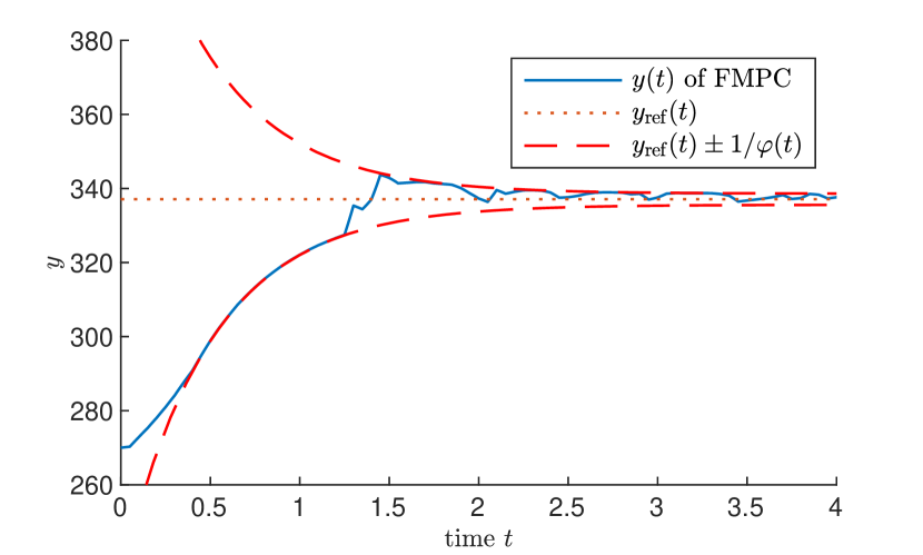
(a) Funnel and system output

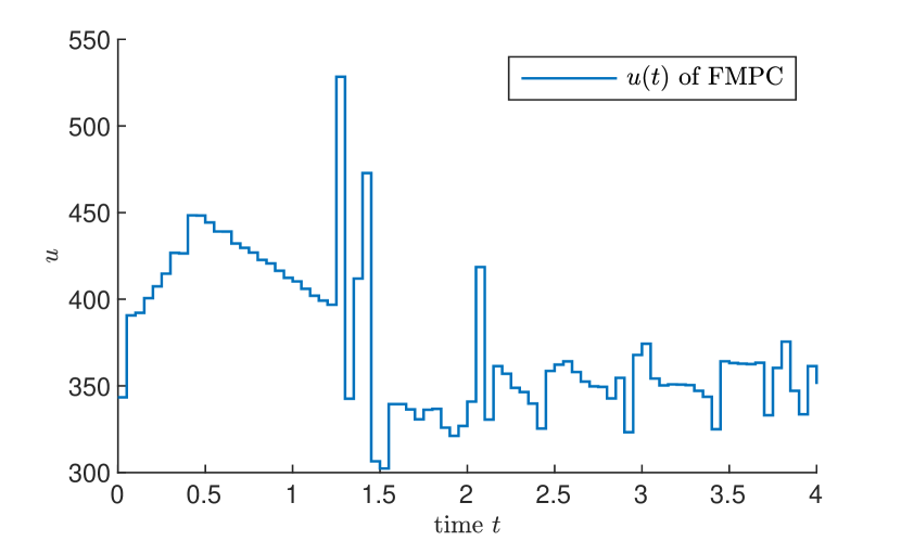
(b) Input signal

Figure 2: Simulation of system (17) under the feedback law (14) of the FMPC Algorithm 2.9.

Figure 3 shows the system output and the control signal if the classical MPC scheme 2.2 with cost function $\ell$ as in (3) and constraints (4) is applied to system (17) instead of the FMPC Algorithm 2.9, with the same parameters, prediction horizon and discretisation.

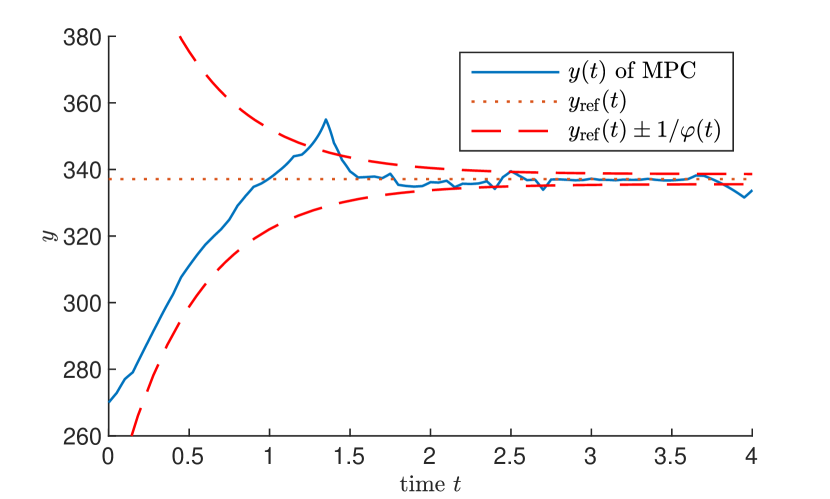
(a) Funnel and system output

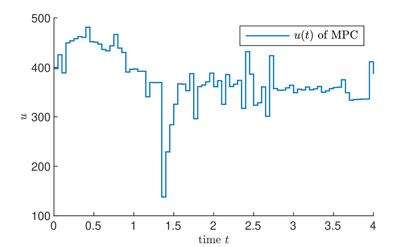
(b) Input signal

Figure 3: Simulation of system (17) under the classical MPC scheme 2.2.

This control does not achieve the control objective since the tracking error exceeds the funnel boundaries. Further adaptation of the parameter $\lambda_{u}$ is necessary in order to ensure that MPC with the corresponding OCP (5) is feasible with this prediction horizon and discretisation. Such tuning of parameters in order to guarantee feasibility is not necessary for the FMPC Algorithm 2.9 since the stage cost function $\ell_{\varphi}$ is automatically increasing, if the tracking error is close to the funnel boundary.

The original funnel controller proposed in [14] takes the form

$$u(t) =-\frac{1}{1-\varphi(t)^{2}\left\|e(t)\right\|^{2}}e(t).$$ (18)

To compare the funnel controller (18) with the FMPC Algorithm 2.9, we chose the prediction horizon and time shift as $T=1$ and $\delta=0.1$, resp. Further, the parameter $\lambda_{u}=\tfrac{1}{10}$ for the cost functional $\ell_{\varphi}$ and a maximal control value of $M=600$ were selected.

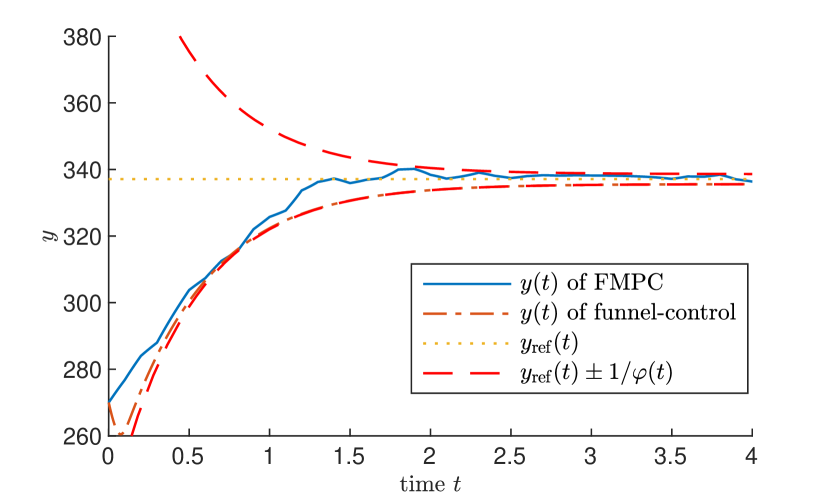
(a) Funnel and tracking errors

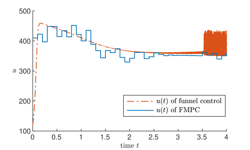
(b) Input functions

Figure 4: Simulation of system (17) under controller (18) and FMPC Algorithm 2.9.

The performance of the funnel controller (18) and the FMPC Algorithm 2.9 is depicted in Figure 4. While Figure 4(a) shows the tracking error of the two controllers evolving within the funnel boundaries, Figure 4(b) shows the respective input signals. It is evident that both control techniques are feasible and achieve the control objective. The input signal of the funnel controller starts to oscillate at $t=2$ and the amplitude of this oscillation increases abruptly at $t=3.5$. This behaviour is caused by a too low sampling rate of the control signal. A relative error tolerance (RelTol) of $2.5\cdot 10^{-7}$ was used. With an even higher sampling rate, this oscillation can be avoided. If a larger error tolerance is used instead, this oscillation behaviour becomes worse. The funnel controller becomes infeasible if the sampling rate is too low (RelTol $>8\cdot 10^{-6}$). The FMPC Algorithm 2.9 does not show this problematic behaviour. Although FMPC uses a relatively wide step of $0.1$ and therefore adapts its control signal significantly less often than the funnel controller, FMPC is feasible and the tracking error evolves within the performance funnel.

3.2 Mass-on-car system

In this section we like to present some promising preliminary results on an extension of the FMPC Algorithm 2.9 to a larger systems class. For that we introduce the general notion of relative degree for system (1). Recall that the Lie derivative of $h$ along $f$ is defined by

$$\left(L_{f}h\right)(x)=\left(\sum_{i=1}^{n}\frac{\partial h_{j}}{\partial x_{i}}(x)\,f_{i}(x)\right)_{j=1,\ldots,n}=h^{\prime}(x)f(x),$$

and we may successively define $L_{f}^{k}h=L_{f}(L_{f}^{k-1}h)$ with $L_{f}^{0}h=h$. Furthermore, for the matrix-valued function $g$ we have

$$(L_{g}h)(x)=\left[(L_{g_{1}}h)(x),\ldots,(L_{g_{m}}h)(x)\right],$$

where $g_{i}$ denotes the $i$-th column of $g$ for $i=1,\ldots,m$. Then system (1) is said to have (global) relative degree $r\in\mathbb{N}$, if

$$\ \forall\,k\in\{1,\ldots,r-1\}\ \forall\,x\in\mathds{R}^{n}:\ (L_{g}L_{f}^{k-1}h)(x)=0\quad\wedge\quad(L_{g}L_{f}^{r-1}h)(x)\in\text{GL}_{m}(\mathds{R}),$$

see [16, Sec. 5.1]. The generalised high-frequency gain matrix is defined as

$$\Gamma(x):=\left(L_{g}L_{f}^{r-1}h\right)(x)\in\text{GL}_{m}(\mathds{R}),\quad x\in\mathds{R}^{n}.$$ (19)

Example 3.2.

The linear system (15) of Example 3.1 has global relative degree $r\in\mathds{N}$ with ${r>1}$, if

$$\ \forall\,\;k\in\{1,\ldots,r-1\}:\ CA^{k-1}B=0\quad\wedge\quad CA^{r-1}B\in\text{GL}_{m}(\mathds{R}).$$

In other words, the relative degree is the number of times the output has to be differentiated in order for the input to appear explicitly on the right side of the equation.

For purposes of illustration that Funnel MPC shows promising results for this larger class of systems with fixed relative degree $r\in\mathds{N}$ we consider the example of a mass-spring system mounted on a car from [26] and compare FMPC with the funnel controller presented in [2]. This example was also examined in [2] and [3] to compare different versions of funnel control. The mass $m_{2}$ moves on a ramp inclined by the angle $\vartheta\in[0,\frac{\pi}{2})$ and mounted on a car with mass $m_{1}$, see Figure 5.

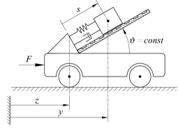
Figure 5: Mass-on-car system.

It is possible to control the force $u$ acting on the car. The motion of the system is described by the equations

$$\begin{bmatrix}m_{1}+m_{2}&m_{2}\cos(\vartheta)\\ m_{2}\cos(\vartheta)&m_{2}\end{bmatrix}\begin{pmatrix}\ddot{z}(t)\\ \ddot{s}(t)\end{pmatrix}+\begin{pmatrix}0\\ ks(t)+d\dot{s}(t)\end{pmatrix}=\begin{pmatrix}u(t)\\ 0\end{pmatrix},$$ (20)

where $z(t)$ is the horizontal position of the car and $s(t)$ the relative position of the mass on the ramp at time $t$. The physical constants $k>0$ and $d>0$ are the coefficients of the spring and damper, resp. The horizontal position of the mass on the ramp is the output $y$ of the system, i.e.,

$$y(t)=z(t)+s(t)\cos(\vartheta).$$

By setting $\mu:=m_{2}(m_{1}+m_{2}\sin^{2}(\vartheta))$, $\mu_{1}=\frac{m_{1}}{\mu}$, and $\mu_{2}=\frac{m_{2}}{\mu}$, the system takes the form (15), with

$$x(t):=\begin{pmatrix}z(t)\\ \dot{z}(t)\\ s(t)\\ \dot{s}(t)\\ \end{pmatrix}\!,\,A:=\begin{bmatrix}0&1&0&0\\ 0&0&\mu_{2}k\cos(\vartheta)&\mu_{2}d\cos(\vartheta)\\ 0&0&0&1\\ 0&0&-(\mu_{1}+\mu_{2})k&-(\mu_{1}+\mu_{2})d\\ \end{bmatrix}\!,\,B:=\begin{bmatrix}0\\ \mu_{2}\\ 0\\ -\mu_{2}\cos(\vartheta)\\ \end{bmatrix}\!,\,C:=\begin{bmatrix}1\\ 0\\ \cos(\vartheta)\\ 0\\ \end{bmatrix}^{\top}\!.$$

It is easy to see that the system has global relative degree $r$ with

$$r=\begin{dcases}2,&\vartheta\in\left(0,\tfrac{\pi}{2}\right)\\ 3,&\vartheta=0\end{dcases}$$

and the scalar high-frequency gain $\Gamma=CA^{r-1}B$ is positive.

We choose the same parameters $m_{1}=4$, $m_{2}=1$, $k=2$, $d=1$, and initial values $z(0)=s(0)=\dot{z}(0)=\dot{s}(0)=0$ as in [2]. The objective is tracking of the reference signal $y_{\operatorname*{ref}}:t\mapsto\cos(t)$, such that for $\varphi\in\mathcal{G}$ the error function $t\mapsto e(t):=y(t)-y_{\operatorname*{ref}}(t)$ evolves within the prescribed performance funnel, i.e., $\varphi(t)\left\|e(t)\right\|<1$ for all $t\geq 0$.

Case 1: If $0<\vartheta<\frac{\pi}{2}$, then the system (20) has relative degree $r=2$. The funnel controller presented in [2] takes the form

$$w(t) =\varphi(t)\dot{e}(t)+\alpha(\varphi(t)^{2}e(t)^{2})\varphi(t)e(t),$$ (21)

$$u(t) =-\alpha(w(t)^{2})w(t),$$

with $\alpha(s)=\frac{1}{1-s}$ for $s\in[0,1)$. Due to discretisation, only step functions with constant step length $0.04$ are considered for the OCP (13) of the FMPC Algorithm 2.9. The prediction horizon and time shift are selected as $T=0.6$ and $\delta=0.04$, resp. We further choose the parameter $\lambda_{u}=\tfrac{1}{100}$ for the stage cost $\ell_{\varphi}$ and allow a maximal control value of $M=30$. As in [2], the funnel function $\varphi(t)=\left(5\mathrm{e}^{-2t}+0.1\right)^{-1}$, $t\geq 0$, is chosen and the case $\vartheta=\tfrac{\pi}{4}$ is considered. All simulations are performed on the time interval $[0,10]$ with the MATLAB routine ode45.

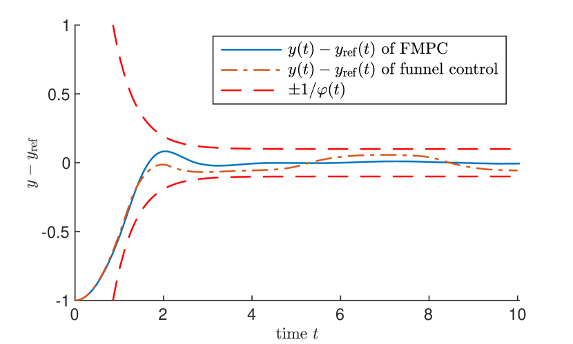
(a) Funnel and tracking errors

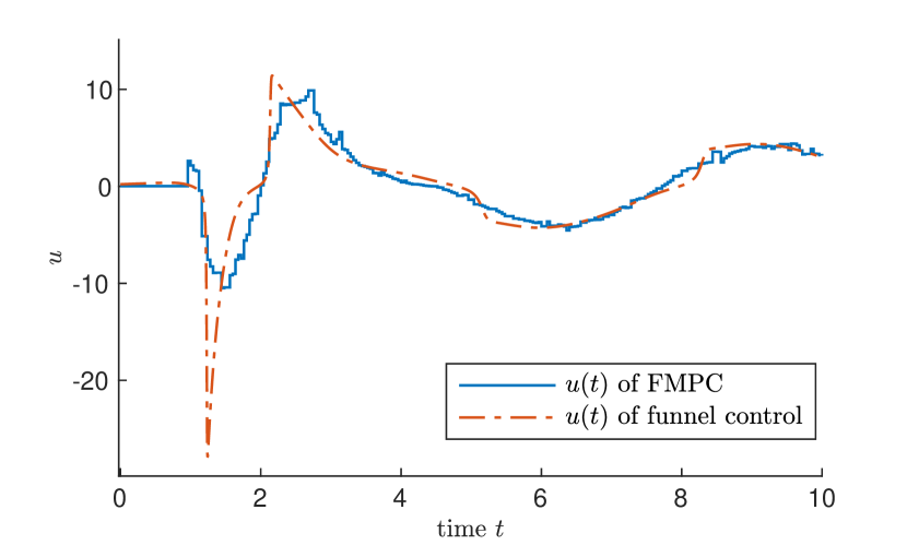
(b) Input functions

Figure 6: Simulation of system (20) with $\vartheta=\tfrac{\pi}{4}$ under controller (21) and FMPC Algorithm 2.9.

The performance of the funnel controller (21) and the FMPC Algorithm 2.9 is depicted in Figure 6. While Figure 6(a) shows the tracking error of the two controllers evolving within the funnel boundaries, Figure 6(b) shows the respective input signals. It is evident that both control techniques are feasible and achieve the control objective. The funnel controller is able to generate a smooth input signal, while the OCP (13) of the FMPC Algorithm 2.9 is optimized over step functions with constant step length $0.04$. Nevertheless, it seems that the FMPC Algorithm achieves a more accurate tracking of the reference signal $y_{\operatorname*{ref}}$ and, at the same time, exhibits a smaller range of employed control values. Funnel control tends to change the control values very quickly and the control signal shows spikes. The FMPC algorithm, however, avoids this due to prediction of the future system behaviour. Similarly to [3], we observed that feasibility of the funnel controller (21) is not maintained for a sampling rate $\tau=\frac{1}{300}$. Instead $\tau=\frac{1}{500}$ turns out to be sufficient. The FMPC Algorithm 2.9 is feasible for both sampling rates. Since the funnel controller needs a far higher sampling rate than FMPC and needs to be able to adapt its control signal very quickly, whereas FMPC uses constant steps with a relatively long length, funnel control exhibits more demanding hardware requirements to stay feasible in application than FMPC

When the classical MPC Algorithm 2.2 with OCP (5) is applied to the system (20) with the same parameters, prediction rate and step length instead of the FMPC Algorithm 2.9, then the tracking error leaves the performance funnel and hence the control objective is not achieved (see Figure 7). Furthermore, the control signal exhibits quite severe peaks.

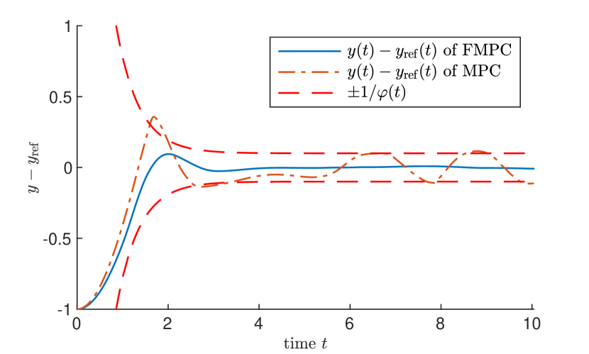
(a) Funnel and tracking errors

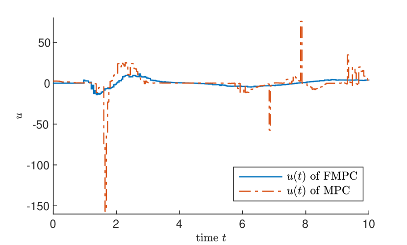
(b) Input functions

Figure 7: Simulation of system (20) with $\vartheta=\tfrac{\pi}{4}$ under a classical MPC scheme 2.2 with OCP (5) and the FMPC Algorithm 2.9.

A possible explanation may be that the constraint $\left\|y(t)-y_{\operatorname*{ref}}(t)\right\|\leq\frac{1}{\varphi(t)}$ of the OCP (5) does not influence the control value as long as it is satisfied, and when the error is close to the funnel boundary, it is too late for the controller to react. The controller attempts to compensate this by generating very large control signals. The FMPC algorithm is able to avoid this behaviour by reacting in advance to a close funnel boundary, because a small distance is penalised by the stage cost. Further adaptation of the parameter $\lambda_{u}$, a smaller step length, or a longer prediction horizon are necessary in order to guarantee feasibility of the classical MPC scheme 2.2. Figure 8 depicts the simulation of the classical MPC scheme with such adapted parameter ($\lambda_{u}=\tfrac{1}{4450}$) in comparison to the FMPC algorithm with the same parameters as before. With these tuned parameters, the classical MPC 2.2 scheme achieves the control objective and the error evolves within the funnel boundaries.

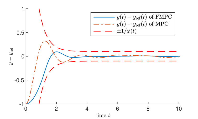
(a) Funnel and tracking errors

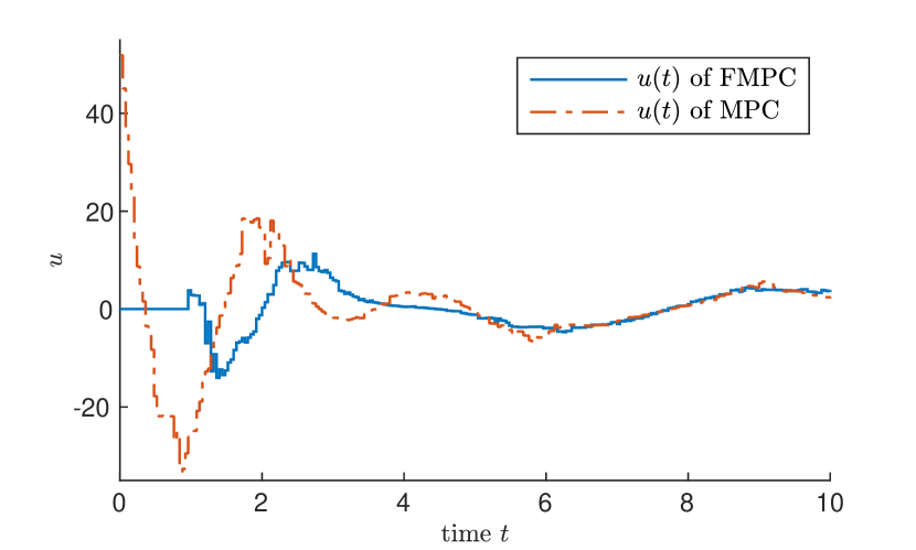
(b) Input functions

Figure 8: Simulation of system (20) with $\vartheta=\tfrac{\pi}{4}$ under the FMPC Algorithm 2.9 and classical MPC 2.2 with OPC (5) and $\lambda_{u}=\frac{1}{4450}$.

Case 2: If $\vartheta=0$, then the system (20) has relative degree $r=3$. The funnel controller from [2] takes the form

$$w(t) =\varphi(t)\ddot{e}(t)+\gamma(\varphi(t)\dot{e}(t)+\gamma(\varphi(t)e(t))),$$ (22)

$$u(t) =-\gamma(w(t)),$$

where $\gamma(s)=\frac{s}{1-s^{2}}$ for $s\in[0,1)$. The OCP (13) of the FMPC Algorithm 2.9 is solved over step functions with constant step length $\tfrac{1}{15}$. The prediction horizon is $T=1$ and the time shift is $\delta=\tfrac{1}{15}$. We further choose the parameter $\lambda_{u}=\frac{1}{100}$ for the stage cost $\ell_{\varphi}$ and allow a maximal control value of $M=30$. As in [2], we choose the funnel function $\varphi(t)=\left(3\mathrm{e}^{-t}+0.1\right)^{-1}$, $t\geq 0$.

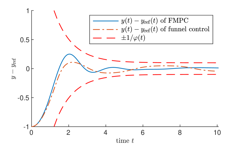
(a) Funnel and tracking errors

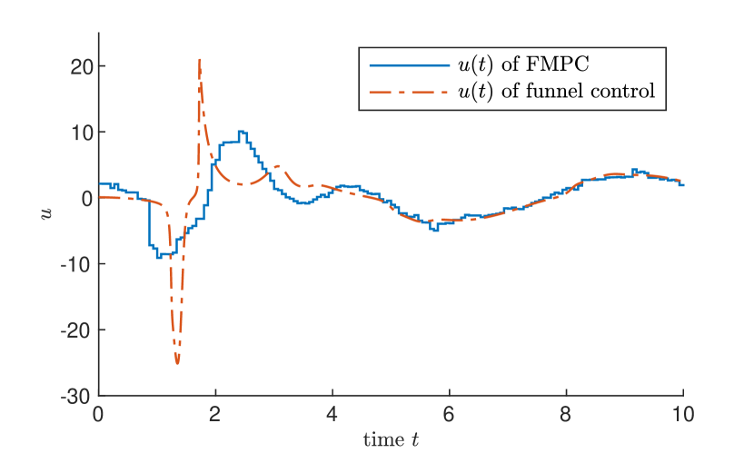
(b) Input functions

Figure 9: Simulation of system (20) with $\vartheta=0$ under controller (22) and FMPC Algorithm 2.9.

The performance of the funnel controller (22) and the FMPC Algorithm 2.9 are depicted in Figure 9. The results are similar to the first case with relative degree $r=2$. Note that the funnel controllers (21) and (22) are structurally different due to the altered relative degree $r$, whereas the FMPC Algorithm 2.9 is the same in both cases. This is of particular relevance when the relative degree $r$ is not known a priori. The above simulations suggest that the FMPC Algorithm 2.9 also works for systems with higher relative degree and exhibits a promising performance.

4 Proof of the main result 2.6

4.1 Optimal control problems with funnel-like stage costs

Before proving initial and recursive feasibility of the Funnel MPC Algorithm 2.2, we show that, by using the stage cost function $\ell_{\varphi}$ as in $\eqref{eq:stageCostFunnelMPC}$, the optimization problem (13) has a solution and that this solution, if applied to the system (1), guarantees that the error $e(t)=y(t)-y_{\operatorname*{ref}}(t)$ evolves within the performance funnel $\mathcal{F}_{\varphi}$. To that end we define, for $T>0$, $M>0$, $t^{0}\in\mathds{R}_{\geq 0}$, and $x^{0}\in\mathds{R}^{n}$, the associated Optimal Control Problem (OCP)

$$\mathop{\operatorname{minimize}}_{\begin{subarray}{c}u\in L^{\infty}([t^{0},t^{0}+T],\mathds{R}^{m}),\\ \left\|u\right\|_{\infty}\leq M\end{subarray}}\quad\int_{t^{0}}^{t^{0}+T}\ell_{\varphi}(t,x(t;t^{0},x^{0},u),u(t))\ \text{d}t.$$ (23)

If the Lebesgue integral in (23) does not exist for some $u\in L^{\infty}([t^{0},t^{0}+T],\mathds{R}^{m})$ with $\left\|u\right\|_{\infty}\leq M$ (i.e., both the Lebesgue integrals of the positive and negative part of $\ell_{\varphi}(\cdot,x(\cdot;t^{0},x^{0},u),u(\cdot))$ are infinite), then its value is treated as infinity. This may happen when $\varphi(t)\left\|h(x(t;t^{0},x^{0},u))-y_{\operatorname*{ref}}(t)\right\|=1$ for some $t\in[t^{0},t^{0}+T]$. If the set of all such points does not have Lebesgue measure zero, then the integral is treated as infinity as well.

We like to point out that there is a subtle difference between a Lebesgue integrable function (which belongs to $L^{1}$) and a function for which the Lebesgue integral exists (which does not need to be in $L^{1}$). To make this difference clearer we call a measurable function $\zeta:B\to\mathds{R}$ on a Borel set $B\subseteq\mathds{R}$ quasi-integrable, if for $\zeta^{+}:=\max\{\zeta,0\}$ and $\zeta^{-}:=\max\{-\zeta,0\}$ at least one of the Lebesgue integrals

$$\int_{B}\zeta^{+}(t)\ \text{d}t\qquad\text{or}\qquad\int_{B}\zeta^{-}(t)\ \text{d}t$$

is finite.

Proposition 2.7 guarantees that, if the funnel controller (12) is applied to the system (1) with initial value $x^{0}\in\mathcal{D}^{\varphi}_{t^{0}}$, then the tracking error evolves in the interior of the funnel. It is not directly clear that this also holds true if a solution of the optimization problem (23) is applied to the system (1). If the initial error is inside the funnel, then it might still be possible that the error $e$ touches or even exceeds the boundary and evolves outside of the funnel boundary after some time. In [3] this issue was resolved by appending state constraints to the optimal control problem. In the following we show that such constraints are unnecessary. In fact, if an arbitrary control function $u\in L^{\infty}([t^{0},t^{0}+T],\mathds{R}^{m})$ such that $\ell_{\varphi}(\cdot,x(\cdot;t^{0},x^{0},u),u(\cdot))$ is quasi-integrable over $[t^{0},t^{0}+T]$ is applied to the system, then it is guaranteed that the error $e$ evolves within the funnel. To show this, an elementary lemma is proved first.

Lemma 4.1.

Let $T>0$ and $g:[0,T]\to\mathds{R}_{\geq 0}$ be Lipschitz continuous. If $\int_{0}^{T}\frac{1}{g(s)}\ \text{d}s<\infty$, then $g(t)>0$ for all $t\in[0,T]$.

Proof.

First assume that there exists $\tau\in(0,T)$ such that $g(\tau)=0$. Choose $\varepsilon>0$ such that ${(\tau-\varepsilon,\tau+\varepsilon)\subset[0,T]}$. Since $g$ is Lipschitz continuous, we have that

$$\ \exists\,C>0\ \forall\,s\in(\tau-\varepsilon,\tau+\varepsilon):\ g(s)=\left|g(s)-g(\tau)\right|\leq C\left|s-\tau\right|.$$

Therefore,

$$\infty>\int_{0}^{T}\frac{1}{g(s)}\ \text{d}s\geq\int_{\tau-\varepsilon}^{\tau+\varepsilon}\frac{1}{g(s)}\ \text{d}s\geq\int_{\tau-\varepsilon}^{\tau+\varepsilon}\frac{1}{C\left|s-\tau\right|}\ \text{d}s=\int_{-\varepsilon}^{\varepsilon}\frac{1}{C\left|s\right|}\ \text{d}s=\infty,$$

a contradiction. A similar proof applies in the cases $\tau=0$ and $\tau=T$. ∎

Remark 4.2.

Lemma 4.1 is not true for all uniformly continuous functions in general. Consider the example:

$$\int_{0}^{1}\frac{1}{\sqrt{x}}\ \text{d}x=2\sqrt{x}\Big{|}_{0}^{1}=2.$$

Theorem 4.3.

Consider system (1) with $(f,g,h)\in\mathcal{N}^{m}$. Let $\varphi\in\mathcal{G},\ y_{\operatorname*{ref}}\in W^{1,\infty}(\mathds{R}_{\geq 0},\mathds{R}^{m})$, $T>0$ $M>0$, $t^{0}\in\mathds{R}_{\geq 0}$, and $x^{0}\in\mathds{R}^{n}$ be given such that ${\mathcal{U}^{\varphi}_{T}(M,t^{0},x^{0})\neq\emptyset}$. Then the following identities hold:

$$\mathcal{U}^{\varphi}_{T}(M,t^{0},x^{0}) =\left\{\ \!\!u\in\mathcal{U}_{T}(t^{0},x)\!\ \left|\ \vphantom{\!\!u\in\mathcal{U}_{T}(t^{0},x)\!}\!\!\!\begin{array}[]{l}\ell_{\varphi}(\cdot,x(\cdot;t^{0},x^{0},u),u(\cdot))\ \text{quasi-integrable on $[t^{0},t^{0}+T]$},\\ \int_{t^{0}}^{t^{0}+T}\ell_{\varphi}(t,x(t;t^{0},x^{0},u),u(t))\,{\rm d}t<\infty,\ \text{and}\ \left\|u\right\|_{\infty}\leq M\end{array}\!\!\!\!\ \right.\right\}$$

$$=\left\{\ \!\!u\in\mathcal{U}_{T}(t^{0},x)\!\ \left|\ \vphantom{\!\!u\in\mathcal{U}_{T}(t^{0},x)\!}\!\!\!\begin{array}[]{l}\ell_{\varphi}(\cdot,x(\cdot;t^{0},x^{0},u),u(\cdot))\in L^{1}([t^{0},t^{0}+T],\mathds{R}),\\ \ell_{\varphi}(\cdot,x(\cdot;t^{0},x^{0},u),u(\cdot))\geq 0,\ \text{and}\ \left\|u\right\|_{\infty}\leq M\\ \end{array}\!\!\!\!\ \right.\right\}$$

Proof.

Given $u\in\mathcal{U}^{\varphi}_{T}(M,t^{0},x^{0})$, it follows from the definition of $\mathcal{U}^{\varphi}_{T}(M,t^{0},x^{0})$ that

$$\varphi(t)\left\|h(x(t;t^{0},x^{0},u))-y_{\operatorname*{ref}}(t)\right\|<1$$

for all $t\in[t^{0},t^{0}+T]$. Define $e(t):=h(x(t;t^{0},x^{0},u))-y_{\operatorname*{ref}}(t)$. Due to continuity of $h,\varphi,y_{\operatorname*{ref}}$, and $x(\cdot;t^{0},x^{0},u)$, there exists $\varepsilon\in(0,1)$ with $\varphi(t)^{2}\left\|e(t)\right\|^{2}<1-\varepsilon$ for all $t\in[t^{0},t^{0}+T]$. Then, $\ell_{\varphi}(t,x(t;t^{0},x^{0},u),u(t))\geq 0$ for all $t\in[t^{0},t^{0}+T]$ and

$$\int_{t^{0}}^{t^{0}+T}\left|\ell_{\varphi}(t,x(t;t^{0},x^{0},u),u(t))\right|\ \text{d}{t} =\int_{t^{0}}^{t^{0}+T}\left|\frac{1}{1-\varphi(t)^{2}\left\|e(t)\right\|^{2}}-1+\lambda_{u}\left\|u(t)\right\|^{2}\right|\ \text{d}{t}$$

$$\leq\int_{t^{0}}^{t^{0}+T}{\frac{1}{\varepsilon}-1+\lambda_{u}\left\|u\right\|_{\infty}^{2}}\ \text{d}{t}\leq\left(\frac{1}{\varepsilon}-1+\lambda_{u}M^{2}\right)T<\infty.$$

Therefore, $\ell_{\varphi}(\cdot,x(\cdot;t^{0},x^{0},u),u(\cdot))\in L^{1}([t^{0},t^{0}+T],\mathds{R})$ and so $\mathcal{U}^{\varphi}_{T}(M,t^{0},x^{0})$ is contained in both of the other two sets in the statement of the theorem.

Let $u\in\mathcal{U}_{T}(t^{0},x)$ with $\left\|u\right\|_{\infty}<M$ and quasi-integrable $\ell_{\varphi}(\cdot,x(\cdot;t^{0},x^{0},u),u(\cdot))$ such that $\int_{t^{0}}^{t^{0}+T}\ell_{\varphi}(t,x(t;t^{0},x^{0},u),u(t))\,{\rm d}t<\infty$ be given. We now show that the error $e(t):=h(x(t;t^{0},x^{0},u))-y_{\operatorname*{ref}}(t)$ satisfies $\varphi(t)\left\|e(t)\right\|<1$ for all $t\in[t^{0},t^{0}+T]$. We already know $x^{0}\in\mathcal{D}^{\varphi}_{t^{0}}$ since ${\mathcal{U}^{\varphi}_{T}(M,t^{0},x^{0})\neq\emptyset}$, i.e., $\varphi(t^{0})\left\|e(t^{0})\right\|<1$. Assume there exists $t\in(t^{0},T]$ with $\varphi(t)\left\|e(t)\right\|\geq 1$. By continuity of $x(\cdot;t^{0},x^{0},u)$,$\varphi$, $h$, and $y_{\operatorname*{ref}}$ there exists

$$\widehat{t}:=\min\left\{\ \tau\in(t^{0},t^{0}+T]\ \left|\ \vphantom{\tau\in(t^{0},t^{0}+T]}\ \varphi(\tau)\left\|e(\tau)\right\|=1\ \right.\right\}.$$

Note that $\varphi(t)\left\|e(t)\right\|<1$ for all $t\in[t^{0},\widehat{t})$. Since $\ell_{\varphi}(\cdot,x(\cdot;t^{0},x^{0},u),u(\cdot))$ is quasi-integrable and $\int_{t^{0}}^{t^{0}+T}\ell_{\varphi}(t,x(t;t^{0},x^{0},u),u(t))\,{\rm d}t<\infty$ it follows that the set $\left\{\ t\in[t^{0},t^{0}+T]\ \left|\ \vphantom{t\in[t^{0},t^{0}+T]}\varphi(t)\left\|e(t)\right\|=1\ \right.\right\}$ has Lebesgue measure zero and

$$\int_{t^{0}}^{t^{0}+T}\big{(}\ell_{\varphi}(t,x(t;t^{0},x^{0},u),u(t))\big{)}^{+}\,{\rm d}t<\infty.$$

Therefore,

$$\int_{t^{0}}^{t^{0}+T}\left(\frac{1}{1-\varphi(t)^{2}\left\|e(t)\right\|^{2}}-1+\lambda_{u}\left\|u(t)\right\|^{2}\right)^{+}\ \text{d}{t}=\int_{t^{0}}^{t^{0}+T}\big{(}\ell_{\varphi}(t,x(t;t^{0},x^{0},u),u(t))\big{)}^{+}<\infty.$$

Invoking $\|u\|_{\infty}\leq M$, this yields $\int_{t^{0}}^{t^{0}+T}\left(\frac{1}{1-\varphi(t)^{2}\left\|e(t)\right\|^{2}}\right)^{+}\ \text{d}{t}<\infty$ and thus

$$\int_{t^{0}}^{\widehat{t}}\frac{1}{1-\varphi(t)^{2}\left\|e(t)\right\|^{2}}\ \text{d}{t}=\int_{t^{0}}^{\widehat{t}}\left(\frac{1}{1-\varphi(t)^{2}\left\|e(t)\right\|^{2}}\right)^{+}\ \text{d}{t}\leq\int_{t^{0}}^{t^{0}+T}\left(\frac{1}{1-\varphi(t)^{2}\left\|e(t)\right\|^{2}}\right)^{+}\ \text{d}{t}<\infty.$$

Since $\varphi\in W^{1,\infty}(\mathds{R}_{\geq 0},\mathds{R})$ and $y_{\operatorname*{ref}}\in W^{1,\infty}(\mathds{R}_{\geq 0},\mathds{R}^{m})$, $\varphi$ and $y_{\operatorname*{ref}}$ are Lipschitz continuous and bounded on the interval $[t^{0},\widehat{t}]$. Let $\Phi:\mathds{R}^{n}\to\mathds{R}^{n}$ be a diffeomorphism such that the coordinate transformation $\Phi(x)=(y,\eta)$ puts the system (1) into Byrnes-Isidori form (8), then $\dot{y}$ can be written as

$$\dot{y}(t)=p\left(y(t),\eta(t)\right)+\Gamma\left(\Phi^{-1}\left(y(t),\eta(t)\right)\right)\,u(t),\\$$

where $(y(t),\eta(t))=\Phi(x(t;t^{0},x^{0},u))$ for $t\in[t^{0},t^{0}+T]$. Since $\|e(t)\|\leq\varphi(t)^{-1}$ for all $t\in[t^{0},\widehat{t}]$, the error $e$ is bounded and so $y$ is bounded, too. Hence by the BIBS assumption (9), applied to $\tilde{y}\in L^{\infty}([t^{0},\infty),\mathds{R}^{m})$ defined by $\tilde{y}(t)=y(t)$ for $t\in[t^{0},\hat{t}]$ and $\tilde{y}(t)=y(\hat{t})$ for $t>\hat{t}$, yields that $\tilde{\eta}(\cdot):=\eta(\cdot;t^{0},\eta^{0},\tilde{y})$ is bounded and since $\tilde{\eta}|_{[t^{0},\hat{t}]}=\eta|_{[t^{0},\hat{t}]}$ we have that $\eta$ is bounded on $[t^{0},\hat{t}]$. Thus, since $p$, $\Gamma$, and $\Phi^{-1}$ are continuous, $\dot{y}$ is essentially bounded on $[t^{0},\hat{t}]$. This implies the Lipschitz continuity of $y$. Products and sums of Lipschitz continuous functions on a compact interval are again Lipschitz continuous. Therefore, $1-\varphi(\cdot)^{2}\left\|e(\cdot)\right\|^{2}=1-\varphi(\cdot)^{2}\left\|y(\cdot)-y_{\operatorname*{ref}}(\cdot)\right\|^{2}$ is Lipschitz continuous on $[t^{0},\widehat{t}]$ and, according to Lemma 4.1, strictly positive. This contradicts the definition of $\widehat{t}$. Hence $\mathcal{U}^{\varphi}_{T}(M,t^{0},x^{0})$ contains the second set in the statement of the theorem. Since the third set is itself contained in the second one the proof is complete. ∎

We are now in the position to define for $T>0$, $t^{0}\in\mathds{R}_{\geq 0}$, $x^{0}\in\mathds{R}^{n}$, and $\ell_{\varphi}$ as in (11) the cost functional

$$J^{\varphi}_{T}(\cdot;t^{0},x^{0}):L^{\infty}([t^{0},t^{0}+T],\mathds{R}^{m})\to\mathds{R}\cup\{\infty\},$$ (24)

$$u\mapsto\begin{dcases}\int_{t^{0}}^{t^{0}+T}\!\!\!\!\!\!\ell_{\varphi}(t,x(t;t^{0},x^{0},u),u(t))\ \text{d}t,&\begin{array}[]{l}\text{$u\in\mathcal{U}_{T}(t^{0},x)$ and}\\ \text{$\ell_{\varphi}(\cdot,x(\cdot;t^{0},x^{0},u),u(\cdot))$ quasi-integrable}\end{array}\\ \infty,&\text{otherwise.}\end{dcases}$$

Although we know that for every $u\in L^{\infty}([t^{0},t^{0}+T],\mathds{R}^{m})$ there exists a unique maximal solution $x(\cdot;t^{0},x^{0},u):[t^{0},\omega)\to\mathds{R}^{n}$ of the system (1), this solution might have finite escape time even before $t^{0}+T$, i.e., $\omega<t^{0}+T$. In this case, and whenever the stage costs $\ell_{\varphi}(\cdot,x(\cdot;t^{0},x^{0},u),u(\cdot))$ are not quasi-integrable, $J^{\varphi}_{T}(u;t^{0},x^{0})=\infty$. In the following remark we state some immediate consequences of this definition and Theorem 4.3.

Remark 4.4.

The following statements hold under the assumptions of Theorem 4.3:

1. $0\leq J^{\varphi}_{T}(u;t^{0},x^{0})<\infty$  for all $u\in\mathcal{U}^{\varphi}_{T}(M,t^{0},x^{0})$.

2. $\mathcal{U}^{\varphi}_{T}(M,t^{0},x^{0})=\left\{\ u\in L^{\infty}([t^{0},t^{0}+T],\mathds{R}^{m})\ \left|\ \vphantom{u\in L^{\infty}([t^{0},t^{0}+T],\mathds{R}^{m})}\left\|u\right\|_{\infty}\leq M,\ J^{\varphi}_{T}(u;t^{0},x^{0})<\infty\ \right.\right\}$.

3. The optimal control problem (23) can be reformulated as

   $$\mathop{\operatorname{minimize}}_{\begin{subarray}{c}u\in L^{\infty}([t^{0},t^{0}+T],\mathds{R}^{m}),\\ \left\|u\right\|_{\infty}\leq M\end{subarray}}J^{\varphi}_{T}(u;t^{0},x^{0}).$$

Remark 4.5.

As opposed to FMPC, barrier function based MPC (see e.g. [32]) uses (relaxed) logarithmic barrier functions to penalise states close to the boundaries of the constraints. Although this might seem to be a subtle difference, this choice has remarkable implications. Lemma 4.1 is a consequence of the non-integrability of $\tfrac{1}{x}$ over the interval $[0,1]$. As pointed out in Remark 4.4, as result of this, a finite value of the cost function ensures that the tracking error $e:=y-y_{\text{ref}}$ remains within the prescribed funnel boundaries. The logarithm on the other hand is integrable over the interval $[0,1]$:

$$\int_{0}^{1}\ln(x^{n})\text{d}x=\underbrace{\ln(x^{n})x\Big{|}_{0}^{1}}_{=0}-\int_{0}^{1}x\frac{n}{x}\text{d}x=-n.$$

Therefore, such a cost function alone can in general not guarantee that the state always remain within the desired region and therefore the usage of terminal conditions (costs and constraints) remains necessary.

If the initial value $x^{0}$ is within the set $\mathcal{D}^{\varphi}_{t^{0}}$, then any control $u$ with $J^{\varphi}_{T}(u;t^{0},x^{0})<\infty$ guarantees that, if applied to the system (1), the error $e(t)=y(t)-y_{\operatorname*{ref}}(t)$ remains strictly within the funnel. Since $J^{\varphi}_{T}(u;t^{0},x^{0})$ is positive for all control functions $u\in\mathcal{U}^{\varphi}_{T}(M,t^{0},x^{0})$, this raises the question as to whether there exists an optimal $u^{\star}$ which minimizes $J^{\varphi}_{T}(\cdot;t^{0},x^{0})$ and is a solution to the optimal control problem (23). The answer is affirmative and shown in the next theorem.

Theorem 4.6.

Consider system (1) with $(f,g,h)\in\mathcal{N}^{m}$. Let $\varphi\in\mathcal{G},\ y_{\operatorname*{ref}}\in W^{1,\infty}(\mathds{R}_{\geq 0},\mathds{R}^{m})$, $T>0$, $M>0$, $t^{0}\in\mathds{R}_{\geq 0}$, and $x^{0}\in\mathcal{D}^{\varphi}_{t^{0}}$ such that ${\mathcal{U}^{\varphi}_{T}(M,t^{0},x^{0})\neq\emptyset}$. Then, there exists a function $u^{\star}\in\mathcal{U}^{\varphi}_{T}(M,t^{0},x^{0})$ such that

$$J^{\varphi}_{T}(u^{\star};t^{0},x^{0})=\min_{u\in\mathcal{U}^{\varphi}_{T}(M,t^{0},x^{0})}J^{\varphi}_{T}(u;t^{0},x^{0})=\min_{\begin{subarray}{c}u\in L^{\infty}([t^{0},t^{0}+T],\mathds{R}^{m}),\\ \left\|u\right\|_{\infty}\leq M\end{subarray}}J^{\varphi}_{T}(u;t^{0},x^{0}).$$

Proof.

The proof essentially follows the lines of [25, Prop. 2.2].
To simplify the notation, assume without loss of generality that $t^{0}=0$ and consider only the interval $[0,T]$. It follows from Remark 4.4 that $J^{\varphi}_{T}(u;t^{0},x^{0})\geq 0$ for all $u\in\mathcal{U}^{\varphi}_{T}(M,t^{0},x^{0})$. Hence the infimum $J^{\star}:=\inf_{u\in\mathcal{U}^{\varphi}_{T}(M,t^{0},x^{0})}J^{\varphi}_{T}(u;t^{0},x^{0})$ exists. Let $(u_{k})\in(\mathcal{U}^{\varphi}_{T}(M,t^{0},x^{0}))^{\mathds{N}}$ be a minimizing sequence, meaning $J^{\varphi}_{T}(u_{k};t^{0},x^{0})\to J^{\star}$. By definition of $\mathcal{U}^{\varphi}_{T}(M,t^{0},x^{0})$, we have $\left\|u_{k}\right\|_{\infty}\leq M$ for all $k\in\mathds{N}$. Since $L^{\infty}([0,T],\mathds{R}^{m})\subseteq L^{2}([0,T],\mathds{R}^{m})$, we conclude that $(u_{k})$ is a bounded sequence in the Hilbert space $L^{2}$, thus there exists a function $u^{\star}\in L^{2}([0,T],\mathds{R}^{m})$ and a weakly convergent subsequence $u_{k}\rightharpoonup u^{\star}$ (which we do not relabel). More precisely, $u_{k}|_{[0,t]}\rightharpoonup u^{\star}|_{[0,t]}$ weakly in $L^{2}([0,t],\mathds{R}^{m})$ for all $t\in[0,T]$ as a straightforward argument shows. We define $(x_{k}):=(x(\cdot;t^{0},x^{0},u_{k}))\in C([0,T],\mathds{R}^{n})^{\mathds{N}}$ as the sequence of associated responses.

Step 1: We show that $(x_{k})$ is uniformly bounded. By $u_{k}\in\mathcal{U}^{\varphi}_{T}(M,t^{0},x^{0})$ we have $x_{k}(t)\in\mathcal{D}_{t}^{\varphi}$, i.e., ${\varphi(t)\left\|h(x_{k}(t))-y_{\operatorname*{ref}}(t)\right\|<1}$ for all $t\in[0,T]$. Set $(y_{k}(t),\eta_{k}(t))=\Phi(x_{k}(t))$ for $t\in[0,T]$ and $k\in\mathds{N}$, where $\Phi:\mathds{R}^{n}\to\mathds{R}^{n}$ is a diffeomorphism such that the coordinate transformation $\Phi(x)=(y,\eta)$ puts the system (1) into Byrnes-Isidori form (8). Since $\varphi$ is positive on $[0,T]$, we obtain

$$\ \forall\,t\in[0,T]:\quad\left\|y_{k}(t)\right\|\leq\left\|h(x_{k}(t))-y_{\operatorname*{ref}}(t)\right\|+\left\|y_{\operatorname*{ref}}(t)\right\|\leq\sup_{t\in[0,T]}\varphi(t)^{-1}+\left\|y_{\operatorname*{ref}}\right\|_{\infty}=:\tilde{c}_{0}$$

and $c_{0}:=\tilde{c}_{0}+\left\|\Phi(x^{0})\right\|$ is independent of $k$. Hence, by (9) there exists $c_{1}>0$ such that

$$\ \forall\,y\in L^{\infty}(\mathds{R}_{\geq 0},\mathds{R}^{m}):\quad\|y\|_{\infty}\leq\tilde{c}_{0}\ \implies\ \|\eta(\cdot;0,\eta_{k}(0),y)\|_{\infty}\leq c_{1}.$$

Extending $y_{k}$ to $\mathds{R}_{\geq 0}$ such that $\|y_{k}\|_{\infty}\leq\tilde{c}_{0}$ then yields that $\|\eta_{k}(t)\|\leq c_{1}$ for all $t\in[0,T]$. Therefore,

$$x_{k}(t)\in\Phi^{-1}\left(\left\{\ \begin{pmatrix}z_{1}\\ z_{2}\end{pmatrix}\in\mathds{R}^{m}\times\mathds{R}^{n-m}\ \left|\ \vphantom{\begin{pmatrix}z_{1}\\ z_{2}\end{pmatrix}\in\mathds{R}^{m}\times\mathds{R}^{n-m}}\left\|z_{1}\right\|\leq\tilde{c}_{0}\ \wedge\ \left\|z_{2}\right\|\leq c_{1}\ \right.\right\}\right)=:\mathcal{K}$$

for all $t\in[0,T]$ and all $k\in\mathds{N}$, where $\mathcal{K}$ is compact and independent of $k$. Hence, $(x_{k})$ is uniformly bounded.

Step 2: We show that $(x_{k})$ is uniformly equicontinuous. Since the sequence $(u_{k})$ is bounded, $M:=\sup_{k\in\mathds{N}}\left\|u_{k}\right\|_{L^{2}}$ exists. Set $C_{1}:=\max_{x\in\mathcal{K}}\left\|f(x)\right\|$ and $C_{2}:=\max_{x\in\mathcal{K}}\left\|g(x)\right\|$, which exist by continuity of $f$ and $g$. Now let $\varepsilon>0$ and define $\delta:=\min\left\{1,\frac{1}{\varepsilon}(C_{1}+MC_{2})\right\}$. Let $k\in\mathds{N}$ and $t_{1},t_{2}\in[0,T]$ such that $|t_{2}-t_{1}|<\delta^{2}$. Then, using Hölder’s inequality in the third estimate,

$$\left\|x_{k}(t_{2})-x_{k}(t_{1})\right\| \leq\int_{t_{1}}^{t_{2}}\left\|f(x_{k}(s))\right\|+\left\|g(x_{k}(s))\right\|\left\|u_{k}(s)\right\|\ \text{d}s$$

$$\leq C_{1}\left|t_{2}-t_{1}\right|+C_{2}\int_{t_{1}}^{t_{2}}\left\|u_{k}(s)\right\|\ \text{d}s$$

$$\leq C_{1}\sqrt{\left|t_{2}-t_{1}\right|}+C_{2}\sqrt{\left|t_{2}-t_{1}\right|}\left\|u_{k}\right\|_{L^{2}}$$

$$\leq C_{1}\sqrt{\left|t_{2}-t_{1}\right|}+C_{2}\sqrt{\left|t_{2}-t_{1}\right|}M$$

$$<\delta(C_{1}+MC_{2})\leq\varepsilon,$$

which shows that $(x_{k})$ is uniformly equicontinuous.

Step 3: By the Arzelà-Ascoli theorem there exists a function $x^{\star}\in\mathcal{C}([0,T],\mathds{R}^{n})$ and a uniformly convergent subsequence $x_{k}\to x^{\star}$ (which we do not relabel). Now we prove that $x^{\star}=x(\cdot;t^{0},x^{0},u^{\star})$, which means to show that

$$x^{\star}(t)=x^{0}+\int_{0}^{t}f(x^{\star}(s))+g(x^{\star}(s))u^{\star}(s)\ \text{d}s,\quad t\in[0,T].$$

We have

$$x_{k}(t)=x^{0}+\int_{0}^{t}f(x_{k}(s))+g(x_{k}(s))u_{k}(s)\ \text{d}s,\quad k\in\mathds{N},\ t\in[0,T],$$

and since $x_{k}$ in particular converges pointwise to $x^{\star}$ and the sequence $(f(x_{k}))$ is uniformly bounded as $(x_{k})$ is uniformly bounded and $f$ is continuous, the bounded convergence theorem gives that

$$\ \forall\,t\in[0,T]:\ \int_{0}^{t}f(x_{k}(s))\ \text{d}s\longrightarrow\int_{0}^{t}f(x^{\star}(s))\ \text{d}s.$$

Therefore, it remains to show

$$\ \forall\,t\in[0,T]:\ \int_{0}^{t}g(x_{k}(s))u_{k}(s)\ \text{d}s\longrightarrow\int_{0}^{t}g(x^{\star}(s))u^{\star}(s)\ \text{d}s.$$

The argument $s$ is omitted in the following. Since $g(x^{\star})$ is bounded on $[0,T]$, it is an element of $L^{2}([0,T],\mathds{R}^{n\times m})$, thus the weak convergence of $(u_{k})$ implies

$$\ \forall\,t\in[0,T]:\ \int_{0}^{t}g(x^{\star})u_{k}\ \text{d}s\longrightarrow\int_{0}^{t}g(x^{\star})u^{\star}\ \text{d}s.$$

Therefore, using Hölder’s inequality in the second estimate we obtain, for all $t\in[0,T]$,

$$\left\|\int_{0}^{t}\!\!\!g(x_{k})u_{k}-g(x^{\star})u^{\star}\!\ \text{d}s\right\| =\left\|\int_{0}^{t}\!\!\!g(x_{k})u_{k}+g(x^{\star})u_{k}-g(x^{\star})u_{k}-g(x^{\star})u^{\star}\!\ \text{d}s\right\|$$

$$\leq\int_{0}^{t}\!\!\!\left\|g(x_{k})-g(x^{\star})\right\|\left\|u_{k}\right\|\!\!\!\ \text{d}s+\left\|\int_{0}^{t}g(x^{\star})u_{k}-g(x^{\star})u^{\star}\!\ \text{d}s\right\|$$

$$\leq\left(\int_{0}^{t}\!\!\!\left\|g(x_{k})-g(x^{\star})\right\|^{2}\!\!\!\ \text{d}s\right)^{\!\frac{1}{2}}\!\!\left(\int_{0}^{t}\!\!\!\left\|u_{k}\right\|^{2}\!\!\!\ \text{d}s\right)^{\!\frac{1}{2}}\!\!\!\!+\left\|\int_{0}^{t}\!\!\!g(x^{\star})u_{k}-g(x^{\star})u^{\star}\!\!\ \text{d}s\right\|$$

$$\leq\sup_{m\in\mathds{N}}\!\left\|u_{m}\right\|_{L^{2}}\!\!\underbrace{\left(\int_{0}^{t}\!\!\!\left\|g(x_{k})-g(x^{\star})\right\|^{2}\!\!\ \text{d}s\!\right)^{\!\frac{1}{2}}\!\!}_{\to 0}\!+\underbrace{\left\|\int_{0}^{t}\!\!\!g(x^{\star})u_{k}-g(x^{\star})u^{\star}\!\ \text{d}s\right\|}_{\to 0}\!\to\!0.$$

Step 4: We show $\left\|u^{\star}\right\|_{\infty}\leq M$. To this end, define the sets

$$A_{m}:=\left\{\ t\in[0,T]\ \left|\ \vphantom{t\in[0,T]}\left\|u^{\star}(t)\right\|^{2}\geq M^{2}+\frac{1}{m}\ \right.\right\},\quad m\in\mathds{N}.$$

Let $\chi_{A_{m}}$ denote the indicator function of the set $A_{m}$, then, since $u_{k}\rightharpoonup u^{\star}$, we have that

$$\langle u_{k},\chi_{A_{m}}u^{\star}\rangle_{L^{2}}\to\langle u^{\star},\chi_{A_{m}}u^{\star}\rangle_{L^{2}}=\|\chi_{A_{m}}u^{\star}\|_{L^{2}}^{2}.$$

On the other hand, by the Cauchy-Schwarz inequality we have that

$$\langle u_{k},\chi_{A_{m}}u^{\star}\rangle_{L^{2}}\leq\|\chi_{A_{m}}u_{k}\|_{L^{2}}\|\chi_{A_{m}}u^{\star}\|_{L^{2}},$$

thus

$$\|\chi_{A_{m}}u^{\star}\|_{L^{2}}=\|\chi_{A_{m}}u^{\star}\|_{L^{2}}^{-1}\liminf_{k\to\infty}\langle u_{k},\chi_{A_{m}}u^{\star}\rangle_{L^{2}}\leq\liminf_{k\to\infty}\|\chi_{A_{m}}u_{k}\|_{L^{2}}$$

and hence

$$\int_{A_{m}}\|u^{\star}(s)\|^{2}\ \text{d}s\leq\liminf_{k\to\infty}\int_{A_{m}}\|u_{k}(s)\|^{2}\ \text{d}s.$$

Since $\|u_{k}\|_{\infty}\leq M$, we then find the following for all $m\in\mathds{N}$ and $k\in\mathds{N}$:

$$\lambda\left(A_{m}\right)=\int_{A_{m}}1\ \text{d}s\leq m\int_{A_{m}}\left\|u^{\star}(s)\right\|^{2}-M^{2}\ \text{d}s\leq m\int_{A_{m}}\left\|u^{\star}(s)\right\|^{2}-\left\|u_{k}(s)\right\|^{2}\ \text{d}s,$$

where $\lambda$ denotes the Lebesgue measure, thus

$$0\leq\lambda\left(A_{m}\right)\leq\liminf_{k\to\infty}m\int_{A_{m}}\left\|u^{\star}(s)\right\|^{2}-\left\|u_{k}(s)\right\|^{2}\ \ \text{d}s\leq 0.$$

Due to the $\sigma$-continuity of $\lambda$ we get

$$\lambda(\left\{\ t\in[0,T]\ \left|\ \vphantom{t\in[0,T]}\left\|u^{\star}(t)\right\|>M\ \right.\right\})=\lambda\left(\bigcup_{m\in\mathds{N}}A_{m}\right)=\lim_{m\to\infty}\lambda(A_{m})=0.$$

This implies $\left\|u^{\star}\right\|_{\infty}\leq M$.

Step 5: We prove $u^{\star}\in\mathcal{U}^{\varphi}_{T}(M,t^{0},x^{0})$, which means to show $x^{\star}(t)\in\mathcal{D}_{t}^{\varphi}$ for all $t\in[0,T]$. Assume there exists $\tau\in(0,T]$ with $\varphi(\tau)\left\|h(x^{\star}(\tau))-y_{\operatorname*{ref}}(\tau)\right\|\geq 1$. By continuity of $x^{\star}$, $\varphi$, $h$, and $y_{\operatorname*{ref}}$ there exists

$$\widehat{t}:=\min\left\{\ \tau\in(0,T]\ \left|\ \vphantom{\tau\in(0,T]}\ \varphi(\tau)\left\|h(x^{\star}(\tau))-y_{\operatorname*{ref}}(\tau)\right\|=1\ \right.\right\}.$$

$\dot{x}^{\star}$ is bounded on the interval $[0,T]$ since $g$ and $f$ are continuous and both $x^{\star}$ and $u^{\star}$ are bounded. Hence, $x^{\star}$ is Lipschitz continuous with Lipschitz constant $L^{\star}>0$. Define the continuously differentiable function $\omega:[0,T]\times\mathcal{K}\to\mathds{R},(t,x)\mapsto 1-\varphi(t)^{2}\left\|h(x)-y_{\operatorname*{ref}}(t)\right\|^{2}$. Due to the compactness of $[0,T]$ and $\mathcal{K}$, $\omega$ is Lipschitz continuous with Lipschitz constant $L_{\omega}>0$. We have $\omega(s,x_{k}(s))>0$ for all $k\in\mathds{N}$ and all $s\in[0,\hat{t}]$ because $u_{k}\in\mathcal{U}^{\varphi}_{T}(M,t^{0},x^{0})$. Since $w(\widehat{t},x^{\star}(\widehat{t}))=0$, the following holds for all $s\in[0,\widehat{t}]$ and all $k\in\mathds{N}$.

$$\omega(s,x_{k}(s)) =\left|\omega(s,x_{k}(s))\right|=\left|\omega(s,x_{k}(s))-w(\widehat{t},x^{\star}(\widehat{t}))\right|$$

$$\leq L_{\omega}\left\|\begin{pmatrix}s-\widehat{t}\\ x_{k}(s)-x^{\star}(\widehat{t})\end{pmatrix}\right\|=L_{\omega}\left\|\begin{pmatrix}s-\widehat{t}\\ x_{k}(s)-x^{\star}(s)+x^{\star}(s)-x^{\star}(\widehat{t})\end{pmatrix}\right\|$$

$$\leq L_{\omega}\left|s-\widehat{t}\right|+L_{\omega}\left\|x_{k}(s)-x^{\star}(s)\right\|+L_{\omega}L^{\star}\left|s-\widehat{t}\right|.$$

The supremum $\sup_{k\in\mathds{N}}J^{\varphi}_{T}(u_{k};t^{0},x^{0})<\infty$ exists because $J^{\varphi}_{T}(u_{k};t^{0},x^{0})\to J^{\star}$. Since $\int_{0}^{\widehat{t}}\tfrac{1}{(L_{\omega}+L_{\omega}L^{\star})\left|s-\widehat{t}\right|}\ \text{d}s=\infty$, there exists $\delta>0$ with $\int_{0}^{\widehat{t}}\tfrac{1}{(L_{\omega}+L_{\omega}L^{\star})\left|s-\widehat{t}\right|+L_{\omega}\delta}\ \text{d}s-\widehat{t}>\sup_{k\in\mathds{N}}J^{\varphi}_{T}(u_{k};t^{0},x^{0})$. Due to the uniform convergence of $x_{k}$ to $x^{\star}$, there exists $K\in\mathds{N}$ such that $\left\|x_{k}(s)-x^{\star}(s)\right\|<\delta$ for all $k\geq K$ and all $s\in[0,\widehat{t}]$. Thus, we arrive, for $k\geq K$, at the following contradiction.

$$\sup_{k\in\mathds{N}}J^{\varphi}_{T}(u_{k};t^{0},x^{0}) \geq\int_{0}^{T}\ell_{\varphi}(s,x_{k}(s),u_{k}(s))\ \text{d}s$$

$$=\int_{0}^{T}\frac{1}{1-\varphi(s)^{2}\left\|h(x_{k}(s))-y_{\operatorname*{ref}}(s)\right\|^{2}}-1+\lambda_{u}\left\|u_{k}(s)\right\|^{2}\ \text{d}s$$

$$\geq\int_{0}^{\widehat{t}}\frac{1}{\omega(s,x_{k}(s))}-1\ \text{d}s$$

$$\geq\int_{0}^{\widehat{t}}\frac{1}{(L_{\omega}+L_{\omega}L^{\star})\left|s-\widehat{t}\right|+L_{\omega}\left\|x_{k}(s)-x^{\star}(s)\right\|}\ \text{d}s-\widehat{t}$$

$$>\int_{0}^{\widehat{t}}\frac{1}{(L_{\omega}+L_{\omega}L^{\star})\left|s-\widehat{t}\right|+L_{\omega}\delta}\ \text{d}s-\widehat{t}>\sup_{k\in\mathds{N}}J^{\varphi}_{T}(u_{k};t^{0},x^{0}).$$

Hence, $u^{\star}\in\mathcal{U}^{\varphi}_{T}(M,t^{0},x^{0})$.

Step 6: We show $J^{\varphi}_{T}(u^{\star};t^{0},x^{0})=J^{\star}$. Let $\tilde{\ell}_{\varphi}:\mathcal{D}^{\varphi}\to\mathds{R},(t,x)\mapsto\tfrac{1}{1-\varphi(t)^{2}\left\|h(x)-y_{\operatorname*{ref}}(t)\right\|^{2}}-1$. For all $k\in\mathds{N}$, we have $\left\|\tilde{\ell}_{\varphi}(\cdot,x_{k}(\cdot))\right\|_{\infty}<\infty$ and $\left\|\tilde{\ell}_{\varphi}(\cdot,x^{\star}(\cdot))\right\|_{\infty}<\infty$ because ${u_{k},u^{\star}\in\mathcal{U}^{\varphi}_{T}(M,t^{0},x^{0})}$. According to Step 5, there exists $\varepsilon>0$ such that $\left\|x^{\star}(t)\right\|\leq\tfrac{1}{\varphi(t)}-\varepsilon$ for all $t\in[0,T]$. Due to the uniform convergence of $x_{k}$ to $x^{\star}$, there exists $N\in\mathds{N}$ such that $\left\|x_{k}-x^{\star}\right\|_{\infty}<\tfrac{\varepsilon}{2}$ for $k\geq N$. Thus,

$$\ \forall\,k\geq N\ \forall\,t\in[0,T]:\quad\left\|x_{k}(t)\right\|\leq\left\|x_{k}(t)-x^{\star}(t)\right\|+\left\|x^{\star}(t)\right\|<\frac{1}{\varphi(t)}-\frac{\varepsilon}{2}.$$

Hence, the sequence $\left(\tilde{\ell}_{\varphi}(\cdot,x_{k}(\cdot))^{\tfrac{1}{2}}\right)$ is uniformly bounded. Due to the continuity of $\tilde{\ell}$, the bounded convergence theorem gives that $\tilde{\ell}_{\varphi}(\cdot,x_{k}(\cdot))^{\tfrac{1}{2}}\to\tilde{\ell}_{\varphi}(\cdot,x^{\star}(\cdot))^{\tfrac{1}{2}}$ strongly and, thus, also weakly in $L^{2}([0,T],\mathds{R})$. Since $J^{\varphi}_{T}(u_{k};t^{0},x^{0})\to J^{\star}=\inf_{u\in\mathcal{U}^{\varphi}_{T}(M,t^{0},x^{0})}J^{\varphi}_{T}(u;t^{0},x^{0})$ and since the $L^{2}$-norm is weakly lower semi-continuous, the following holds.

$$J^{\varphi}_{T}(u^{\star};t^{0},x^{0}) =\int_{0}^{T}\ell_{\varphi}(s,x^{\star}(s),u^{\star}(s))\ \text{d}s=\left\|\tilde{\ell}_{\varphi}(\cdot,x^{\star}(\cdot))^{\frac{1}{2}}\right\|_{L^{2}}^{2}+\lambda_{u}\left\|u^{\star}\right\|_{L^{2}}^{2}$$

$$\leq\liminf_{k\to\infty}\left\|\tilde{\ell}_{\varphi}(\cdot,x_{k}(\cdot))^{\frac{1}{2}}\right\|_{L^{2}}^{2}+\liminf_{k\to\infty}\lambda_{u}\left\|u_{k}\right\|_{L^{2}}^{2}\leq\liminf_{k\to\infty}J^{\varphi}_{T}(u_{k};t^{0},x^{0})=J^{\star}.$$

Therefore $J^{\varphi}_{T}(u^{\star};t^{0},x^{0})=\min_{u\in\mathcal{U}^{\varphi}_{T}(M,t^{0},x^{0})}J^{\varphi}_{T}(u;t^{0},x^{0})$.

Step 7: We show that $J^{\varphi}_{T}(u^{\star};t^{0},x^{0})=\min_{\begin{subarray}{c}u\in L^{\infty}([t^{0},t^{0}+T],\mathds{R}^{m}),\\ \left\|u\right\|_{\infty}\leq M\end{subarray}}J^{\varphi}_{T}(u;t^{0},x^{0})$. Since $\mathcal{U}^{\varphi}_{T}(M,t^{0},x^{0})\neq\emptyset$ by assumption this follows from Remark 4.4 (ii) and completes the proof. ∎

4.2 Initial and recursive feasibility

In the following we seek to show initial and recursive feasibility of the FMPC Algorithm 2.9. For this we need to show that the essential assumption $\mathcal{U}^{\varphi}_{T}(M,t^{0},x^{0})\neq\emptyset$ of Theorem 4.6 is initially (i.e., at $t=t^{0}$) and recursively (i.e., at $t=t^{0}+\delta n$ after $n$ steps of Algorithm 2.9) satisfied. The main difficulty is to prove the existence of a number $M>0$ for which the latter is satisfied for all initial values within a prescribed bounded set. This is the purpose of the following results.

First observe that applying the funnel controller (12) from Proposition 2.7 to the system (1) ensures that the error evolves strictly within the funnel for any initial condition $x^{0}\in\mathcal{D}^{\varphi}_{t^{0}}$. As stated in Remark 2.8 the funnel controller is bounded. This bound however depends on the initial value $x^{0}$. This means that for every $x^{0}\in\mathcal{D}^{\varphi}_{t^{0}}$ there exists $M>0$ such that $\mathcal{U}^{\varphi}_{T}(M,t^{0},x^{0})$ is non-empty. This raises the question whether it is possible to find a bound $M$ independent of the initial value $x^{0}$. The following example shows that this is not the case in general.

Example 4.7.

Consider the two-dimensional linear system

$$\dot{y}(t) =\eta(t)+u(t), \qquad y(0) =0,$$

$$\dot{\eta}(t) =0, \qquad\eta(0) =\eta^{0},$$

in Byrnes-Isidori form with constant reference signal $y_{\operatorname*{ref}}\equiv 0$ and the constant funnel $\varphi\equiv 1$. Let $M>0$ and $T>0$ be arbitrary. Although the system satisfies the BIBS condition (9) and the initial error $e(0)=y^{0}-y_{\operatorname*{ref}}(0)=0$ lies within the funnel for every $\eta^{0}\in\mathds{R}$, there exists $\eta^{0}\in\mathds{R}$ such that the error $e$ exceeds the funnel boundaries at time $T$ for every $u\in L^{\infty}([0,T],\mathds{R})$ with $\|u\|_{\infty}\leq M$. To see this, choose $\eta^{0}:=M+\frac{2}{T}$, then

$$e\left(T\right)=y\left(T\right)=\int_{0}^{T}\eta(s)+u(s)\ \text{d}s=T\eta^{0}+\int_{0}^{T}u(s)\ \text{d}s\geq T\eta^{0}-TM=2>1=\frac{1}{\varphi\left(T\right)}.$$

The example shows that, in general, there exists no $M>0$ such that $\mathcal{U}^{\varphi}_{T}(M,t^{0},x^{0})$ is non-empty for all $x^{0}\in\mathcal{D}^{\varphi}_{t^{0}}$. However, for a bounded set $B\subset\mathcal{D}^{\varphi}_{t^{0}}$ of initial values, it is possible to find a uniform bound $M>0$. Moreover, $M$ can be chosen independently of $T>0$. To show this, we denote by $\mathcal{Y}^{\varphi,y^{0}}_{y_{\operatorname*{ref}}}(I)$ the set of all functions in $\mathcal{C}(I,\mathds{R}^{m})$ starting at $y^{0}\in\mathds{R}^{m}$ and evolving within the funnel on an interval $I\subseteq\mathds{R}_{\geq 0}$ of the form $I=[a,b)$ with $b\in(a,\infty]$ or $I=[a,b]$ with $b\in(a,\infty)$:

$$\mathcal{Y}^{\varphi,y^{0}}_{y_{\operatorname*{ref}}}(I):=\left\{\ y\in\mathcal{C}(I,\mathds{R}^{m})\ \left|\ \vphantom{y\in\mathcal{C}(I,\mathds{R}^{m})}y(\inf I)=y^{0},\ \ \forall\,t\in I:\ \varphi(t)\left\|y(t)-y_{\operatorname*{ref}}(t)\right\|<1\ \right.\right\}.$$

Lemma 4.8.

Consider system (1) with $(f,g,h)\in\mathcal{N}^{m}$. Let $\varphi\in\mathcal{G}$, $y_{\operatorname*{ref}}\in W^{1,\infty}(\mathds{R}_{\geq 0},\mathds{R}^{m})$, $t^{0}\in\mathds{R}_{\geq 0}$. Then for all bounded sets $B\subset\mathds{R}^{n}$ there exists a compact set $K\subset\mathds{R}^{n}$ such that

$$\ \forall\,T>0\ \forall\,(y^{0},\eta^{0})\in B\ \forall\,y\in\mathcal{Y}^{\varphi,y^{0}}_{y_{\operatorname*{ref}}}([t^{0},t^{0}+T])\ \forall\,t\in[t^{0},t^{0}+T]:\quad(y(t),\eta(t;t^{0},\eta^{0},y))\in K.$$ (25)

Proof.

Define

$$N_{t}:=\left\{\ \eta(t;t^{0},\eta^{0},y)\ \left|\ \vphantom{\eta(t;t^{0},\eta^{0},y)}(y^{0},\eta^{0})\in B,\ y\in\mathcal{Y}^{\varphi,y^{0}}_{y_{\operatorname*{ref}}}([t^{0},\infty))\ \right.\right\},\quad t\geq t^{0}.$$

By definition of $\mathcal{G}$, $\varphi$ is strictly positive and $\inf_{t\geq 0}\varphi(t)>0$. Therefore, $1/\varphi$ is bounded. Since clearly $y_{\operatorname*{ref}}\in W^{1,\infty}(\mathds{R}_{\geq 0},\mathds{R}^{m})$ is bounded, every function $y\in\mathcal{Y}^{\varphi,y^{0}}_{y_{\operatorname*{ref}}}([t^{0},\infty))$ is bounded by

$$\left\|y\right\|_{\infty}\leq\left\|y-y_{\operatorname*{ref}}\right\|_{\infty}+\left\|y_{\operatorname*{ref}}\right\|_{\infty}\leq\left\|\tfrac{1}{\varphi}\right\|_{\infty}+\left\|y_{\operatorname*{ref}}\right\|_{\infty}.$$

Since $B$ is bounded it follows from the BIBS condition (9) that the set $N:=\bigcup_{t\geq t^{0}}N_{t}$ is also bounded. Furthermore, the set

$$O:=\bigcup_{t\geq t^{0}}\left\{\ y\in\mathds{R}^{m}\ \left|\ \vphantom{y\in\mathds{R}^{m}}\varphi(t)\left\|y-y_{\operatorname*{ref}}(t)\right\|<1\ \right.\right\}$$

is bounded, too. Then the set $K:=\overline{O\times N}$ is compact and by definition of $N$ and $O$ we find that (25) holds. ∎

The following result provides a number $M>0$ with $\mathcal{U}^{\varphi}_{T}(M,t^{0},x^{0})\neq\emptyset$ for all initial values $x^{0}$ from any compact set which satisfies a condition similar to (25).

Proposition 4.9.

Consider system (1) with $(f,g,h)\in\mathcal{N}^{m}$. Let $\varphi\in\mathcal{G}$, $\ y_{\operatorname*{ref}}\in W^{1,\infty}(\mathds{R}_{\geq 0},\mathds{R}^{m})$, $T>0$, $t^{0}\in\mathds{R}_{\geq 0}$, $x^{0}\in\mathcal{D}_{t^{0}}^{\varphi}$, and $\Phi:\mathds{R}^{n}\to\mathds{R}^{n}$ be a diffeomorphism such that the coordinate transformation $\Phi(x)=(y,\eta)$ puts the system (1) into Byrnes-Isidori form (8). Let $(y^{0},\eta^{0})=\Phi(x^{0})$ and $K\subset\mathds{R}^{n}$ be a compact set with

$$\ \forall\,y\in\mathcal{Y}^{\varphi,y^{0}}_{y_{\operatorname*{ref}}}([t^{0},t^{0}+T])\ \forall\,t\in[t^{0},t^{0}+T]:\quad(y(t),\eta(t;t^{0},\eta^{0},y))\in K.$$ (26)

If

$$M\geq G_{\rm max}\left(P_{\rm max}+\left\|\tfrac{\text{d}}{\text{d}t}\tfrac{1}{\varphi}\right\|_{\infty}+\left\|\dot{y}_{\operatorname*{ref}}\right\|_{\infty}\right),$$ (27)

where, with $p(\cdot,\cdot)$ and $\Gamma(\cdot)$ as in (7) and (8),

$$P_{\rm max}:=\max_{(y,\eta)\in K}\|p(y,\eta)\|,\quad G_{\rm max}:=\max_{(y,\eta)\in K}\|\Gamma(\Phi^{-1}(y,\eta))^{-1}\|,$$

then $\mathcal{U}^{\varphi}_{T}(M,t^{0},x^{0})\neq\emptyset$.

Proof.

Step 1: We first show the existence of $M>0$ satisfying (27). Note that $p$ and $\Gamma$ from (7) and (8) are continuous and $\Gamma$ is pointwise invertible. Therefore, $P_{\rm max}$ and $G_{\rm max}$ are well-defined. Furthermore, the essential supremum $\left\|\dot{y}_{\operatorname*{ref}}\right\|_{\infty}$ is finite, because $y_{\operatorname*{ref}}\in W^{1,\infty}(\mathds{R}_{\geq 0},\mathds{R}^{m})$. Since $\varphi$ is an element of $W^{1,\infty}(\mathds{R}_{\geq 0},\mathds{R})$, always positive and $\inf_{t\geq 0}\varphi(t)>0$ the reciprocal $\psi:=1/\varphi$ is an element of $W^{1,\infty}(\mathds{R}_{\geq 0},\mathds{R})$, too, and in particular $\dot{\psi}$ is bounded. Thus, $M$ can be chosen as in (27).

Step 2: We construct a control function $u$ and show that $u\in\mathcal{U}^{\varphi}_{T}(M,t^{0},x^{0})$. To this end, define $e(t):=y(t)-y_{\operatorname*{ref}}(t)$ and observe that, since $x^{0}\in\mathcal{D}_{t^{0}}^{\varphi}$, we have $\varphi(t^{0})\left\|e(t^{0})\right\|<1$. The application of the output feedback

$$u(t)=\Gamma\big{(}\Phi^{-1}(y(t),\eta(t))\big{)}^{-1}\left(-p(y(t),\eta(t))+\varphi(t^{0})e(t^{0})\dot{\psi}(t)+\dot{y}_{\operatorname*{ref}}(t)\right)$$

to the system (8) leads to a closed-loop system. If this initial value problem is considered on the interval $[t^{0},t^{0}+T]$, then there exists a unique maximal solution $(y,\eta):[t^{0},\omega)\to\mathds{R}^{n}$ with $\omega\in(t^{0},t^{0}+T]$ and if $(y,\eta)$ is bounded, then $\omega=t^{0}+T$, cf. [31, § 10, Thm. XX]. Then we find for all $t\in[t^{0},\omega)$ that

$$\left\|e(t)\right\| =\left\|\int_{t^{0}}^{t}\dot{y}(s)-\dot{y}_{\operatorname*{ref}}(s)\ \text{d}s+e(t^{0})\right\|$$

$$=\left\|\int_{t^{0}}^{t}p(y(s),\eta(s))+\Gamma\big{(}\Phi^{-1}(y(s),\eta(s))\big{)}u(s)-\dot{y}_{\operatorname*{ref}}(s)\ \text{d}s+e(t^{0})\right\|$$

$$=\left\|\int_{t^{0}}^{t}\varphi(t^{0})e(t^{0})\dot{\psi}(s)\ \text{d}s+e(t^{0})\right\|=\left\|\varphi(t^{0})e(t^{0})\left(\psi(t)-\psi(t^{0})\right)+e(t^{0})\right\|$$

$$=\underbrace{\varphi(t^{0})\left\|e(t^{0})\right\|}_{<1}\psi(t)<\psi(t).$$

This means, the tracking error $e$ remains within the funnel, i.e., $(y(t),\eta(t))\in\mathcal{D}_{t}^{\varphi}$ for all $t\in[t^{0},\omega)$. Thus, $y$ is uniformly bounded by

$$\left\|y\right\|_{\infty}\leq\left\|y-y_{\operatorname*{ref}}\right\|_{\infty}+\left\|y_{\operatorname*{ref}}\right\|_{\infty}\leq\left\|\psi\right\|_{\infty}+\left\|y_{\operatorname*{ref}}\right\|_{\infty}.$$

Since the error remains within the funnel, the output $y$, defined on $[t^{0},\omega)$, can be extended to an element $\tilde{y}\in\mathcal{Y}^{\varphi,y^{0}}_{y_{\operatorname*{ref}}}([t^{0},t^{0}+T])$ and so by assumption (26) we have

$$\ \forall\,t\in[t^{0},\omega):\quad(y(t),\eta(t;t^{0},\eta^{0},y))\in K.$$

Therefore, $(y,\eta)$ is bounded and hence $\omega=t^{0}+T$ and, with the same arguments, $(y,\eta)$ has a continuous extension to $[t^{0},t^{0}+T]$. Furthermore, by definition of $u$ it is clear that $\|u\|_{\infty}\leq M$ and hence $u\in\mathcal{U}^{\varphi}_{T}(M,t^{0},x^{0})$, which completes the proof. ∎

The result of Proposition 4.9 essentially guarantees initial feasibility of Algorithm 2.9 for all initial values from a given bounded set, which we will summarize in the following theorem. To further obtain recursive feasibility we need to ensure that, after the application of a control $u$ from $\mathcal{U}^{\varphi}_{T}(M,t^{0},x^{0})$ over an interval $[t^{0},t]$, the set of controls corresponding to the new state value, namely $\mathcal{U}^{\varphi}_{T}(M,t,x(t;t^{0},x^{0},u))$, is non-empty as well.

Theorem 4.10.

Consider system (1) with $(f,g,h)\in\mathcal{N}^{m}$. Let $\varphi\in\mathcal{G}$, $\ y_{\operatorname*{ref}}\in W^{1,\infty}(\mathds{R}_{\geq 0},\mathds{R}^{m})$, $t^{0}\in\mathds{R}_{\geq 0}$, and $B\subseteq\mathcal{D}^{\varphi}_{t^{0}}$ be a bounded set. Then, there exists $M>0$ such that

$$\ \forall\,x^{0}\in B\ \forall\,T>0:\quad\mathcal{U}^{\varphi}_{T}(M,t^{0},x^{0})\neq\emptyset$$ (28)

and, furthermore,

$$\ \forall\,x^{0}\in B\ \forall\,T_{1},T_{2}>0\ \forall\,u\in\mathcal{U}^{\varphi}_{T_{1}}(M,t^{0},x^{0})\ \forall\,t\in[t^{0},t^{0}+T_{1}]:\quad\mathcal{U}^{\varphi}_{T_{2}}(M,t,x(t;t^{0},x^{0},u))\neq\emptyset.$$ (29)

Proof.

Let $\Phi:\mathds{R}^{n}\to\mathds{R}^{n}$ be a diffeomorphism such that the coordinate transformation $\Phi(x)=(y,\eta)$ puts the system (1) into Byrnes-Isidori form (8). Fix $x^{0}\in B$ and set $(y^{0},\eta^{0}):=\Phi(x^{0})$. According to Lemma 4.8 there exists a compact set $K$ such that (25) holds. In particular, $K$ satisfies (26) for every $T>0$. Therefore, Proposition 4.9 yields that there exists $M>0$, independent of $x^{0}$, such that $\mathcal{U}^{\varphi}_{T}(M,t^{0},x^{0})\neq\emptyset$ for all $T>0$, which shows (28).

If, for any $T_{1}>0$ an arbitrary but fixed control function $u\in\mathcal{U}^{\varphi}_{T_{1}}(M,t^{0},x^{0})$ is applied to the system (1), then the output $y$ of the system (i.e., $y(\cdot):=h(x(\cdot;t^{0},x^{0},u))$) evolves within the funnel and is therefore an element of $\mathcal{Y}^{\varphi,y^{0}}_{y_{\operatorname*{ref}}}([t^{0},t^{0}+T_{1}])$. By (25), this implies $\Phi(x(t;t^{0},x^{0},u))\in K$ for all $t\in[t^{0},t^{0}+T_{1}]$. If, for any $\widehat{t}\in[t^{0},t^{0}+T_{1}]$, the system is considered on the interval $[\widehat{t},\widehat{t}+T_{2}]$ with $T_{2}>0$ and the current state $x(\widehat{t};t^{0},x^{0},u)$ of the system as initial value, then the prerequisites for Proposition 4.9 are still met on the interval $[\widehat{t},\widehat{t}+T_{2}]$, i.e., $K$ satisfies (26) in the sense

$$\ \forall\,\tilde{y}\in\mathcal{Y}^{\varphi,\widehat{y}}_{y_{\operatorname*{ref}}}([\widehat{t},\widehat{t}+T_{2}])\ \forall\,t\in[\widehat{t},\widehat{t}+T_{2}]:\quad(\tilde{y}(t),\eta(t;\widehat{t},\widehat{\eta},\tilde{y}))\in K,$$

where $(\widehat{y},\widehat{\eta}):=\Phi(x(\widehat{t};t^{0},x^{0},u))\in K$. To see this, observe that for any $\tilde{y}\in\mathcal{Y}^{\varphi,\widehat{y}}_{y_{\operatorname*{ref}}}([\widehat{t},\widehat{t}+T_{2}])$ there exists $\bar{y}\in\mathcal{Y}^{\varphi,y^{0}}_{y_{\operatorname*{ref}}}([t^{0},\widehat{t}+T_{2}])$ with $\bar{y}|_{[\widehat{t},\widehat{t}+T_{2}]}=\tilde{y}$ and $\bar{y}|_{[t^{0},\widehat{t}]}=y$ ($\bar{y}$ is continuous since $y(\widehat{t})=\widehat{y}$) and we have $\eta(t;t^{0},\eta^{0},\bar{y})=\eta(t;\widehat{t},\widehat{\eta},\tilde{y})$ for $t\in[\widehat{t},\widehat{t}+T_{2}]$, thus the assertion follows from (26). Therefore, Proposition 4.9 can again be applied and yields $\mathcal{U}^{\varphi}_{T_{2}}(M,\widehat{t},x(\widehat{t};t^{0},x^{0},u))\neq\emptyset$, which completes the proof. ∎

Example 4.11.

We revisit Example 3.1 and calculate a number $M>0$ satisfying (28) and (29) to illustrate Theorem 4.10 for the linear case. Consider the system (16) in Byrnes-Isidori form with $(A_{1},A_{2},A_{3},A_{4})\in\mathds{R}^{m\times m}\times\mathds{R}^{m\times(n-m)}\times\mathds{R}^{(n-m)\times m}\times\mathds{R}^{(n-m)\times(n-m)}$ and $t^{0}\in\mathds{R}_{\geq 0}$. Let $\varphi\in\mathcal{G}$, $y_{\operatorname*{ref}}\in W^{1,\infty}(\mathds{R}_{\geq 0},\mathds{R}^{m})$ and define $\psi:=1/\varphi$. Further, assume that $A_{4}$ is Hurwitz, i.e., all of its eigenvalues have a negative real part. Then there exist $\alpha>0$, $\beta\geq 1$ such that

$$\ \forall\,x\in\mathds{R}^{n-m}\ \forall\,\text{$t\geq t^{0}$}:\quad\left\|\mathrm{e}^{A_{4}(t-t^{0})}x\right\|\leq\beta\mathrm{e}^{-\alpha(t-t^{0})}\left\|x\right\|.$$

Let $N\subset\mathds{R}^{n-m}$ be an arbitrary, but fixed bounded set. We show that for

$$B:=\left\{\ y\in\mathds{R}^{m}\ \left|\ \vphantom{y\in\mathds{R}^{m}}\varphi(t^{0})\left\|y-y_{\operatorname*{ref}}(t^{0})\right\|<1\ \right.\right\}\times N\subseteq\mathcal{D}^{\varphi}_{t^{0}}$$

and

$$M:=\left\|\Gamma^{-1}\right\|\left(\left(\left\|A_{1}\right\|+\frac{\beta}{\alpha}\left\|A_{2}\right\|\left\|A_{3}\right\|\right)\left(\left\|\psi\right\|_{\infty}+\left\|y_{\operatorname*{ref}}\right\|_{\infty}\right)+\beta\left\|A_{2}\right\|\sup_{\eta^{0}\in N}\left\|\eta_{0}\right\|+\left\|\dot{\psi}\right\|_{\infty}\!\!+\left\|\dot{y}_{\operatorname*{ref}}\right\|_{\infty}\right)$$

the conditions (28) and (29) are satisfied. One can see that $M$ is chosen according to inequality (27) with a more accurate estimate for $P_{\max}$.

To this end, let $T>0$ and $(y^{0},\eta^{0})\in B$ be arbitrary and denote $e(t):=y(t)-y_{\operatorname*{ref}}(t)$. Since the initial value is inside the funnel, we have $\varphi(t^{0})\left\|e(t^{0})\right\|<1$. If the output feedback

$$u(t):=\Gamma^{-1}\left(-A_{1}y(t)-A_{2}\eta(t)+\varphi(t^{0})e(t^{0})\dot{\psi}(t)+\dot{y}_{\operatorname*{ref}}(t)\right)$$

is applied to the system (16), then clearly a unique global solution $(y,\eta):[t^{0},\infty)\to\mathds{R}^{n}$ exists and, as in the proof of Proposition 4.9, we may calculate that $\left\|e(t)\right\|<\psi(t)$ for all $t\geq t^{0}$. As a consequence $(y(t),\eta(t))\in\mathcal{D}_{t}^{\varphi}$ for all $t\geq t^{0}$, and $y$ is uniformly bounded by

$$\left\|y\right\|_{\infty}\leq\left\|y-y_{\operatorname*{ref}}\right\|_{\infty}+\left\|y_{\operatorname*{ref}}\right\|_{\infty}\leq\left\|\psi\right\|_{\infty}+\left\|y_{\operatorname*{ref}}\right\|_{\infty}.$$

Therefore, for $t\geq t^{0}$ we have

$$\left\|\eta(t;t^{0},\eta^{0},y)\right\| =\left\|\mathrm{e}^{A_{4}(t-t^{0})}\eta^{0}+\int_{t^{0}}^{t}\mathrm{e}^{A_{4}(t-s)}A_{3}y(s)\ \text{d}s\right\|$$

$$\leq\left\|\mathrm{e}^{A_{4}(t-t^{0})}\right\|\left\|\eta^{0}\right\|+\int_{t^{0}}^{t}\left\|\mathrm{e}^{A_{4}(t-s)}\right\|\left\|A_{3}\right\|\left\|y(s)\right\|\ \text{d}s$$

$$\leq\beta\mathrm{e}^{-\alpha(t-t^{0})}\sup_{\eta^{0}\in N}\left\|\eta^{0}\right\|+\int_{t^{0}}^{t}\beta\mathrm{e}^{-\alpha(t-t^{0})}\left\|A_{3}\right\|\left(\left\|\psi\right\|_{\infty}+\left\|y_{\operatorname*{ref}}\right\|_{\infty}\right)\ \text{d}s$$

$$\leq\beta\sup_{\eta^{0}\in N}\left\|\eta^{0}\right\|+\left\|A_{3}\right\|\frac{\beta}{\alpha}\left(\left\|\psi\right\|_{\infty}+\left\|y_{\operatorname*{ref}}\right\|_{\infty}\right).$$

As a consequence we see that $\|u\|_{\infty}\leq M$ and thus

$$\ \forall\,T>0:\ u\in\mathcal{U}^{\varphi}_{T}(M,t^{0},(y^{0},\eta^{0}))\neq\emptyset$$

and (28) is satisfied. If any $u\in\mathcal{U}^{\varphi}_{T}(M,t^{0},(y^{0},\eta^{0}))$ is applied to the system (16) and the system is then considered for any $\widehat{t}\in[t^{0},t^{0}+T]$ and $\widehat{T}>0$ on the interval $[\widehat{t},\widehat{t}+\widehat{T}]$, then $\varphi(\widehat{t})\left\|e(\widehat{t})\right\|<1$ and it can be similarly shown that the feedback control

$$\widehat{u}(t):=\Gamma^{-1}\left(-A_{1}y(t)-A_{2}\eta(t)+\varphi(\widehat{t})e(\widehat{t})\dot{\psi}(t)+\dot{y}_{\operatorname*{ref}}(t)\right)$$

leads to an element of $\mathcal{U}^{\varphi}_{\widehat{T}}(M,\widehat{t},x(\widehat{t};t^{0},x^{0},u))$, by which $M$ satisfies (29). Here we like to emphasize that the estimate for $\eta$ needs to be carried out in terms of $t^{0}$, i.e., for $\widehat{y}(t):=h(x(t;\widehat{t},x(\widehat{t};t^{0},x^{0},u),\widehat{u}))$ denoting the output on $[\widehat{t},\widehat{t}+\widehat{T}]$ and $\widehat{\eta}=\eta(\widehat{t};t^{0},x^{0},u)$ we have that

$$\eta(t;\widehat{t},\widehat{\eta},\widehat{y}) =\mathrm{e}^{A_{4}(t-\widehat{t})}\widehat{\eta}+\int_{\widehat{t}}^{t}\mathrm{e}^{A_{4}(t-s)}A_{3}\widehat{y}(s)\ \text{d}s$$

$$=\mathrm{e}^{A_{4}(t-t^{0})}\eta^{0}+\int_{t^{0}}^{\widehat{t}}\mathrm{e}^{A_{4}(t-s)}A_{3}y(s)\ \text{d}s+\int_{\widehat{t}}^{t}\mathrm{e}^{A_{4}(t-s)}A_{3}\widehat{y}(s)\ \text{d}s$$

and hence we obtain the same bound for $\left\|\eta(t;\widehat{t},\widehat{\eta},\widehat{y})\right\|$ as for $\left\|\eta(t;t^{0},\eta^{0},y)\right\|$.

We are now in the position to summarize our results by showing initial and recursive feasibility of the FMPC Algorithm 2.9 and proving Theorem 2.10.

Proof of Theorem 2.10.

Step 1: According to Theorem 4.10, there exists $M>0$ satisfying (28) and (29). Let $x^{0}\in B$ be an arbitrary initial value and $T\geq\delta$. Since $\mathcal{U}^{\varphi}_{T}(M,t^{0},x^{0})\neq\emptyset$ by (28), Theorem 4.6 yields the existence of some $u^{\star}\in\mathcal{U}^{\varphi}_{T}(M,t^{0},x^{0})$ such that $J^{\varphi}_{T}$ has a minimum, that is

$$J^{\varphi}_{T}(u^{\star};t^{0},x^{0})=\min_{\begin{subarray}{c}u\in L^{\infty}([t^{0},t^{0}+T],\mathds{R}^{m}),\\ \left\|u\right\|_{\infty}\leq M\end{subarray}}J^{\varphi}_{T}(u;t^{0},x^{0}),$$

i.e., $u^{\star}$ is a solution of (13) for $\widehat{t}=t^{0}$ and hence the FMPC Algorithm 2.9 is initially feasible. Furthermore, by $u^{\star}\in\mathcal{U}^{\varphi}_{T}(M,t^{0},x^{0})$ we have that the error satisfies $\left\|e(t)\right\|\leq\varphi(t)^{-1}$ for all $t\in[t^{0},t^{0}+\delta)$.

Step 2: Let $\widehat{t}\in t^{0}+\delta\mathds{N}_{0}$ be such that the OCP (13) has a solution $u^{\star}\in\mathcal{U}^{\varphi}_{T}(M,\widehat{t},\widehat{x})$ defined on $[\widehat{t},\widehat{t}+T]$ and let $x:[t^{0},\widehat{t}+\delta)\to\mathds{R}^{n}$ be the solution of (1) under the FMPC feedback (14). We now show that the OCP also has a solution at the next time step $\widehat{t}+\delta$. Since $u^{\star}$ is defined on $[\widehat{t},\widehat{t}+T]$, the solution $x$ has a continuous extension to $[\widehat{t},\widehat{t}+T]$ and, in particular, $\widehat{x}:=x(\widehat{t}+\delta)$ is well defined. With $u_{\rm FMPC}(t)=\mu(t,x(\tilde{t}))$ for $t\in[\tilde{t},\tilde{t}+\delta)$, $\tilde{t}\in t^{0}+\delta\mathds{N}$, $\tilde{t}\leq\widehat{t}$, the corresponding control input $u_{\rm FMPC}$ is well defined on $[t^{0},\widehat{t}+\delta)$ and we have $x(t)=x(t;t^{0},x^{0},u_{\rm FMPC})$ for all $t\in[t^{0},\widehat{t}+\delta)$. Then (29) gives that $\mathcal{U}^{\varphi}_{T}(M,\widehat{t}+\delta,\widehat{x})\neq\emptyset$ and by Theorem 4.6 there exists $\tilde{u}\in\mathcal{U}^{\varphi}_{T}(M,\widehat{t}+\delta,\widehat{x})$ such that $J^{\varphi}_{T}$ has a minimum, that is

$$J^{\varphi}_{T}(\tilde{u};\widehat{t}+\delta,\widehat{x})=\min_{\begin{subarray}{c}u\in L^{\infty}([\widehat{t}+\delta,\widehat{t}+\delta+T],\mathds{R}^{m}),\\ \left\|u\right\|_{\infty}\leq M\end{subarray}}J^{\varphi}_{T}(u;\widehat{t}+\delta,\widehat{x}),$$

hence $\tilde{u}$ is a solution of (13) on $[\widehat{t}+\delta,\widehat{t}+\delta+T]$. Under the feedback (14), the solution $x$ can thus be extended to $[t^{0},\widehat{t}+2\delta)$ and, by definition of $\mathcal{U}^{\varphi}_{T}(M,\widehat{t}+\delta,\widehat{x})$, the corresponding tracking error $e$ satisfies $\left\|e(t)\right\|\leq\varphi(t)^{-1}$ for all $t\in[t^{0},\widehat{t}+2\delta)$. This shows that the FMPC Algorithm 2.9 is recursively feasible.

Step 3: By Step 2 we have shown that system (1) under the FMPC feedback (14) has a global solution $x:[t^{0},\infty)\to\mathds{R}^{n}$ and, since $u_{\rm FMPC}|_{[\widehat{t},\widehat{t}+\delta]}\in\mathcal{U}^{\varphi}_{\delta}(M,\widehat{t},x(\widehat{t}))$ for all $\widehat{t}\in t^{0}+\delta\mathds{N}$, we have that i and ii hold. ∎

5 Conclusion

In the present paper we have shown that the FMPC scheme proposed in [3], which solves the problem of tracking a reference signal within a prescribed performance funnel, is initially and recursively feasible for an arbitrary finite prediction horizon when applied to nonlinear multi-input multi-output systems with relative degree one and stable internal dynamics (in the sense of a BIBS condition). By exploiting concepts from funnel control and using a new “funnel-like” stage cost function, feasibility is achieved without any need for additional terminal or explicit output constraints while also being restricted to (a priori) bounded control values. In particular, we have shown that the additional output constraints in the OCP of FMPC considered in [3] are not required to infer the feasibility results. We have illustrated the application of the FMPC scheme by a simulation not only of relative degree one systems – for which feasibility is proved so far – but also of systems with higher relative degree. The simulations show promising preliminary results for this case, too. It is a subject of future research to show that FMPC is in fact applicable to a larger class of nonlinear systems with stable internal dynamics and higher relative degree.

References

- [1] Emre Aydiner, Matthias A. Müller, and Frank Allgöwer. Periodic reference tracking for nonlinear systems via model predictive control. In 2016 European Control Conference (ECC), pages 2602–2607, 2016.
- [2] Thomas Berger, Achim Ilchmann, and Eugene P. Ryan. Funnel control of nonlinear systems. Math. Control Signals Syst., 33:151–194, 2021.
- [3] Thomas Berger, Carolin Kästner, and Karl Worthmann. Learning-based Funnel-MPC for output-constrained nonlinear systems. IFAC-PapersOnLine, 53(2):5177–5182, 2020.
- [4] Thomas Berger, Svenja Otto, Timo Reis, and Robert Seifried. Combined open-loop and funnel control for underactuated multibody systems. Nonlinear Dynamics, 95:1977–1998, 2019.
- [5] Andrea Boccia, Lars Grüne, and Karl Worthmann. Stability and feasibility of state constrained MPC without stabilizing terminal constraints. Systems & control letters, 72:14–21, 2014.
- [6] Christopher I. Byrnes and Alberto Isidori. Asymptotic stabilization of minimum phase nonlinear systems. IEEE Trans. Autom. Control, 36(10):1122–1137, 1991.
- [7] Jean-Michel Coron, Lars Grüne, and Karl Worthmann. Model predictive control, cost controllability, and homogeneity. SIAM Journal on Control and Optimization, 58(5):2979–2996, 2020.
- [8] Stefano Di Cairano and Francesco Borrelli. Reference tracking with guaranteed error bound for constrained linear systems. IEEE Transactions on Automatic Control, 61(8):2245–2250, 2016.
- [9] Willem Esterhuizen, Karl Worthmann, and Stefan Streif. Recursive feasibility of continuous-time model predictive control without stabilising constraints. IEEE Control Systems Letters, 5(1):265–270, 2020.
- [10] Paola Falugi and David Q Mayne. Getting robustness against unstructured uncertainty: a tube-based mpc approach. IEEE Transactions on Automatic Control, 59(5):1290–1295, 2013.
- [11] Lars Grüne and Jürgen Pannek. Nonlinear Model Predictive Control: Theory and Algorithms. Springer, London, 2017.
- [12] Christoph M. Hackl. Non-identifier Based Adaptive Control in Mechatronics–Theory and Application. Springer-Verlag, Cham, Switzerland, 2017.
- [13] Achim Ilchmann. Non-Identifier-Based High-Gain Adaptive Control. Springer-Verlag, London, 1993.
- [14] Achim Ilchmann, Eugene P. Ryan, and Christopher J. Sangwin. Tracking with prescribed transient behaviour. ESAIM: Control, Optimisation and Calculus of Variations, 7:471–493, 2002.
- [15] Achim Ilchmann and Stephan Trenn. Input constrained funnel control with applications to chemical reactor models. Syst. Control Lett., 53(5):361–375, 2004.
- [16] Alberto Isidori. Nonlinear Control Systems. Springer-Verlag, Berlin, 3rd edition, 1995.
- [17] Johannes Köhler, Matthias A. Müller, and Frank Allgöwer. Nonlinear reference tracking: An economic model predictive control perspective. IEEE Transactions on Automatic Control, 64(1):254–269, 2019.
- [18] Johannes Köhler, Matthias A. Müller, and Frank Allgöwer. A nonlinear model predictive control framework using reference generic terminal ingredients. IEEE Transactions on Automatic Control, 65(8):3576–3583, 2020.
- [19] Johannes Köhler, Raffaele Soloperto, Matthias A Müller, and Frank Allgöwer. A computationally efficient robust model predictive control framework for uncertain nonlinear systems. IEEE Transactions on Automatic Control, 66(2):794–801, 2020.
- [20] Daniel Liberzon and Stephan Trenn. The bang-bang funnel controller. In Proc. 49th IEEE Conf. Decis. Control, Atlanta, USA, pages 690–695, 2010.
- [21] D Limon, JM Bravo, T Alamo, and EF Camacho. Robust mpc of constrained nonlinear systems based on interval arithmetic. IEE Proceedings-Control Theory and Applications, 152(3):325–332, 2005.
- [22] David Q Mayne, María M Seron, and SV Raković. Robust model predictive control of constrained linear systems with bounded disturbances. Automatica, 41(2):219–224, 2005.
- [23] S Joe Qin and Thomas A Badgwell. A survey of industrial model predictive control technology. Control engineering practice, 11(7):733–764, 2003.
- [24] James Blake Rawlings, David Q Mayne, and Moritz Diehl. Model predictive control: theory, computation, and design, volume 2. Nob Hill Publishing Madison, WI, 2017.
- [25] Noboru Sakamoto. When does stabilizability imply the existence of infinite horizon optimal control in nonlinear systems? 2020. arXiv:2008.13387v1.
- [26] Robert Seifried and Wojciech Blajer. Analysis of servo-constraint problems for underactuated multibody systems. Mech. Sci., 4:113–129, 2013.
- [27] Armands Senfelds and Arturs Paugurs. Electrical drive DC link power flow control with adaptive approach. In Proc. 55th Int. Sci. Conf. Power Electr. Engg. Riga Techn. Univ., Riga, Latvia, pages 30–33, 2014.
- [28] Sumeet Singh, Anirudha Majumdar, Jean-Jacques Slotine, and Marco Pavone. Robust online motion planning via contraction theory and convex optimization. In 2017 IEEE International Conference on Robotics and Automation (ICRA), pages 5883–5890. IEEE, 2017.
- [29] HJ Sussmann. Limitations on the stabilizability of globally-minimum-phase systems. IEEE Transactions on automatic control, 35(1):117–119, 1990.
- [30] HJ Sussmann and PV Kokotovic. The peaking phenomenon and the global stabilization of nonlinear systems. IEEE Transactions on automatic control, 36(4):424–440, 1991.
- [31] Wolfgang Walter. Ordinary Differential Equations. Springer-Verlag, New York, 1998.
- [32] Adrian G. Wills and William P. Heath. Barrier function based model predictive control. Automatica, 40(8):1415–1422, 2004.
- [33] Shuyou Yu, Christoph Maier, Hong Chen, and Frank Allgöwer. Tube mpc scheme based on robust control invariant set with application to lipschitz nonlinear systems. Systems & Control Letters, 62(2):194–200, 2013.
- [34] Meng Yuan, Chris Manzie, Malcolm Good, Iman Shames, Farzad Keynejad, and Troy Robinette. Bounded error tracking control for contouring systems with end effector measurements. In 2019 IEEE International Conference on Industrial Technology (ICIT), pages 66–71, 2019.