Episodic Bandits with Stochastic Experts

Abstract

We study a version of the contextual bandit problem where an agent can intervene through a set of stochastic expert policies. The agent interacts with the environment over episodes, with each episode having different context distributions; this results in the ‘best expert’ changing across episodes. Our goal is to develop an agent that tracks the best expert over episodes. We introduce the Empirical Divergence-based UCB (ED-UCB) algorithm in this setting where the agent does not have any knowledge of the expert policies or changes in context distributions. With mild assumptions, we show that bootstrapping from $\mathcal{O}(N\log(NT^{2}\sqrt{E}))$ samples results in a regret of $\mathcal{O}(E(N+1)+\frac{N\sqrt{E}}{T^{2}})$ for $N$ experts over $E$ episodes, each of length $T$. If the expert policies are known to the agent a priori, then we can improve the regret to $\mathcal{O}(EN)$ without requiring any bootstrapping. Our analysis also tightens pre-existing logarithmic regret bounds to a problem-dependent constant in the non-episodic setting when expert policies are known. We finally empirically validate our findings through simulations.

1 Introduction

Recommendation systems for suggesting items to users are commonplace in online services such as marketplaces, content delivery platforms and ad placement systems. Such systems, over time, learn from user feedback, and improve their recommendations. An important caveat, however, is that both the distribution of user types and their respective preferences change over time, thus inducing changes in the optimal recommendation and requiring the system to periodically “reset” its learning.

In this paper, we consider systems with known change-points (aka episodes) in the distribution of user-types and preferences. Examples include seasonality in product recommendations where there are marked changes in interests based on time-of-year, or ad-placements based on time-of-day. While a baseline strategy would be to re-learn the recommendation algorithm in each episode, it is often advantageous to share some learning across episodes. Specifically, one often has access to (potentially, a very) large number of pre-trained recommendation algorithms (aka experts), and the goal then is to quickly determine (in an online manner) which expert is best suited to a specific episode. Crucially, the relationship among these experts can be learned over time – meaning that given samples of (recommended action, reward) from the deployment of one expert, we can infer what the reward would have been if some other expert were used. Such learned “transfer” across experts uses data from all the deployed experts over past episodes, and extracts invariant relationships holding across episodes; while the data collected in each episode, alongside this learned transfer, permits one to quickly determine the episode-dependent best expert.

To motivate the above episodic setting, we take the case of online advertising agencies which are companies that have proprietary ad-recommendation algorithms that place ads for other product companies on newspaper websites based on past campaigns. In each campaign, the agencies places ads for a specific product of the client (eg, a flagship car, gaming consoles, etc) in order to maximize the click-through rate of users on the newspaper website. At any given time, the agency signs contracts for new campaigns with new companies. The information about product features and user profiles form the context, whose distribution changes across campaigns due to change in user traffic and updated product line ups. This could also cause shifts in user preferences. In practice, the agency already has a finite inventory of ad-recommendation models (aka experts, typically logistic models for their very low inference delays of micro-seconds that is mandated by real-time user traffic) from past campaigns. On a new campaign, online ad agencies bid for slots in news media outlets depending on the profile of the user that visits their website, using these pre-learned experts (see [Perlich et al., 2014, Zhang et al., 2014]). In this setting, agencies only re-learn which experts in their inventory works best (and possibly fine tune) for their new campaign. Our work models this episodic setup, albeit, without fine tuning of experts between campaigns.

1.1 Main contributions

We formulate this problem as an Episodic Bandit with Stochastic Experts. Here, an agent interacts with an environment through a set of $N$ experts over $E$ episodes. Each expert $i$ is characterized by a fixed and unknown conditional distribution over actions in a set $\mathcal{V}$ given the context from $\mathcal{X}$. At the start of episode $e$, the context distribution $p_{e}(\cdot)$ as well the distribution of rewards $q_{e}(\cdot|v,x)$ changes and remains fixed over the length of the episode denoted by $T$. At each time, the agent observes the context $X$, chooses one of the $N$ experts and plays the recommended action $V$ to receive a reward $Y$. Note here that the expert policies remain invariant across all episodes.

The goal of the agent is to track the episode-dependent best expert in order to maximize the cumulative sum of rewards. Here, the best expert in a given episode is one that generates the maximum average reward averaged over the randomness in contexts, recommendations and rewards. Due to the stochastic nature of experts, we can use Importance Sampling (IS) estimators to share reward information to leverage the information leakage.

Our main contributions are as follows:

1. Empirical Divergence-Based Upper Confidence Bound (ED-UCB) Algorithm:

We develop the ED-UCB algorithm (Algorithm 1) for the episodic bandit problem with stochastic experts which employs a novel Empirical IS estimator to predict expert rewards using on approximate knowledge of source and target distributions. The design of this estimator is inspired by the Clipped IS estimator of [Sen et al., 2018] used in the D-UCB algorithm. We analyse our Empirical IS estimator, proving exponentially fast concentration into an interval around the true mean in Lemma 2.

For a single episode, we show that using the empirical IS estimator, ED-UCB (with well approximated expert policies) can provide constant average cumulative regret which does not scale with the duration of interaction. Specifically, in Theorem 3, for $N$ experts, we show that ED-UCB incurs a regret of at most $\mathcal{O}(C_{1}N)$ for a problem-dependent constant $C_{1}$. Our analysis also improves the existing regret bounds for D-UCB which promises $\mathcal{O}(N\log T)$ regret in the full information case. In particular, our analysis implies a regret upper bound of $\mathcal{O}(C_{2}N)$ for D-UCB, where $C_{2}$ is another problem-dependent constant.

2. Episodic behavior with bootstrapping:

We also specify the construction of the approximate experts used by ED-UCB in the case when the supports of $X,V$ are finite. We show that if the agent is bootstrapped with $\mathcal{O}(|\mathcal{V}|\log(T)+\log(|\mathcal{X}|NT\sqrt{E}))$ samples per expert, the use of ED-UCB over $E$ episodes, each of length $T$ guarantees a regret bound of $\mathcal{O}\left(E(N+1)+\nicefrac{{N\sqrt{E}}}{{T^{2}}}\right)$ where the dominant term does not scale with $T$. Our regret bound lies in between those of D-UCB in the full information setting and naive optimistic bandit policies (e.g., UCB in [Auer et al., 2002a], KL-UCB in [Cappé et al., 2013]), demonstrating the merits of sharing information among experts. We also mention how our methods can be extended to continuous context spaces.

3. Empirical evaluation:

We validate our findings empirically through simulations on the Movielens 1M dataset [Harper and Konstan, 2015]. We provide soft-control on the genre of the recommendation for users that are clustered according to age and show that the performance of ED-UCB is comparable to that of D-UCB and significantly better than the naive strategies of UCB and KL-UCB.

1.2 Related work

Adapting to changing environments forms the basis of meta-learning [Thrun, 1998, Baxter, 1998] where agents learn to perform well over new tasks that appear in phases but share underlying similarities with the tasks seen in the past. Our approach can be viewed as an instance of meta-learning for bandits, where we are presented with varying environments in each episode with similarities across episodes. Here, the objective is to act to achieve the maximum possible reward through bandit feedback, while also using the past observations (including offline data if present). This setting is studied in [Azar et al., 2013] where a finite hypothesis space maps actions to rewards with each phase having its own true hypothesis. The authors propose an UCB based algorithm that learns the hypothesis space across phases, while quickly learning the true hypothesis in each phase with the current knowledge. Similarly, linear bandits where instances have common unknown but sparse support is studied in [Yang et al., 2020]. In [Cella et al., 2020, Kveton et al., 2021], meta-learning is viewed from a Bayesian perspective where in each phase an instance is drawn from a common meta-prior which is unknown. In particular, [Cella et al., 2020] studies meta-linear bandits and provide regret guarantees for a regularized ridge regression, whereas [Kveton et al., 2021] uses Thompson sampling for general problems, with Bayesian regret bounds for K-armed bandits.

Collective learning in a fixed and contextual environment with bandit feedback, where the reward of various arms and context pairs share a latent structure is known as Contextual Bandits ([Auer et al., 2002b, Chu et al., 2011, Bubeck and Cesa-Bianchi, 2012, Langford and Zhang, 2007, Dudik et al., 2011, Agarwal et al., 2014, Simchi-Levi and Xu, 2020, Deshmukh et al., 2017] among several others), where actions are taken with respect to a context that is revealed in each round. In various works, [Agarwal et al., 2014, Simchi-Levi and Xu, 2020, Foster and Rakhlin, 2020, Foster et al., 2018] a space of hypotheses is assumed to capture the mapping of arms and context pairs to reward, either exactly (realizable setting) or approximately (non-realizable), and bandit feedback is used to find the true hypothesis which provides the greedy optimal action, while adding enough exploration to aid learning.

In the context of online learning, Importance Sampling (IS) is used to transfer knowledge about random quantities under a known target distribution using samples from a known behavior distribution in the context of off-policy evaluation in reinforcement learning [Mahmood et al., 2014]. Clipped IS estimates are also commonly studied in order to reduce the variance of the estimates by introducing a controlled amount of bias [Charles et al., 2013, Bubeck et al., 2013, Lattimore et al., 2016, Sen et al., 2017]. Bootstrapping from prior data has been used in [Zhang et al., 2019] to warm-start the online learning process.

Meta-learning algorithms take a model-based approach, where the invariant-structure (hypothesis space in [Azar et al., 2013] or meta-prior in [Cella et al., 2020, Kveton et al., 2021]) is first learnt to make the optimal decisions, while most contextual bandit algorithms are policy-based, trying to learn the optimal mapping by imposing structure on the policy space. Our approach falls in the latter category of optimizing over policies (aka experts) from a given finite set of policies. However, contrary to the commonly assumed deterministic policies, each policy in our setting is given by fixed distributions over arms conditioned on the context (learnt by bootstrapping from offline data). Using the estimated experts, in each episode (where both the arm reward per context and context distributions change), we quickly learn the average rewards of the experts by collectively using samples from all the experts. In [Sen et al., 2018], a single episode of our setting is considered for the case where policy and context distributions are known to the agent, thus it does not capture episodic learning. Instead, we build on the Importance sampling (IS) approach therein and propose empirical IS by the learning of expert policies via bootstrapping from offline data, and adapting to changing reward and context distributions online. Furthermore, we tighten the single episode regret from logarithmic in episode length to constant.

2 Problem Setup

An agent interacts with a contextual bandit environment through a set of experts $\Pi=\{\pi_{1},...\pi_{N}\}$ over $E$ episodes. In each episode, the distribution from which contexts are drawn changes; we denote $p_{e}(\cdot)$ over a finite set $\mathcal{X}$ to be the context distribution in episode $e\in[E]$. We use $T$ to denote the length of each episode and re-use $1,2,\ldots,T$ to index time in each episode. At each time $t<T$ in episode $e$, a context is drawn independently from $p_{e}$ and revealed to the agent which then selects the expert $\pi_{i_{t}}$ (or simple, expert $i_{t}$) to recommend an action $V_{t}$ from a finite set of actions $\mathcal{V}$. The agent receives a reward $Y_{t}\sim q_{e}(\cdot|X_{t},V_{t})$ based on the context $X_{t}$ and the recommended action $V_{t}$. Given a context $X$, the recommendation of expert $i$ is sampled from the conditional distribution $\pi_{i}(\cdot|X)$. The choice of expert at this time $t$ can be instructed by the set of historical observations $(X_{n},i_{n},V_{n},Y_{n})_{n<t}$ and the current context $X_{t}$. In summary, the context and reward distributions $p_{e},q_{e}$ are allowed to vary over episodes while the expert policies remain invariant and none of these distributions are revealed to the user.

In each episode, the agent seeks to remain competitive with respect to the “best” expert defined as follows: Let $\mu_{i,e}=\mathbb{E}_{i,e}[Y]$ be the mean reward of expert $i\in[N]$ in episode $e\in[E]$. Here, the expectation is taken with respect to the joint distribution $p_{e}(x)\pi_{i}(v|x)q_{e}(y|v,x)$. Then, the best expert in this episode is $i_{e}^{*}=\operatorname*{arg\,max}_{i\in[N]}\mu_{i,e}$ with the maximum average reward $\mu^{*}_{e}=\mu_{i_{e}^{*},e}$. Since the distributions $p_{e},q_{e}$ can vary with episodes, the best expert is also episode-dependent. The agent aims to minimize the cumulative regret across $E$ episodes given by

$$R(T,E)=\sum_{e=1}^{E}\sum_{t=1}^{T_{e}}\mu^{*}_{e}-\mathbb{E}[\mu_{i_{t},e}],$$

where the expectation is over the randomness in the expert-selection process. In this work, we assume that the context and action sets $\mathcal{X},\mathcal{V}$ respectively are finite and rewards are bounded.

2.1 Outline

When expert policies are known a priori, the D-UCB algorithm in [Sen et al., 2018] uses clipped Importance Sampling (IS) based estimators in order to infer the rewards of a particular expert based on samples collected from all the experts. In the absence of such knowledge, the agent uses historical data to estimate these policies and generates estimates of the IS ratio between all expert pairs. These ratio estimates are then used to create an empirical IS estimator for the rewards of a specific expert (target) using the sampled rewards of all the experts. The key technical challenge is then to characterize how the error in the IS ratio estimates affects the reward estimates of the target expert. Specifically, the error in the estimated IS ratio necessitates the clipper levels and the length of the confidence interval of the estimator to be redesigned in order to accommodate the additional bias. Using ratio concentrations, we show exponential concentration bounds of our empirical IS estimator (see Lemma 2).

In Section 3 we consider a single episode and develop the ED-UCB algorithm. We provide the regret analysis in Section 4, providing the constant regret guarantee in Theorem 3 for ED-UCB even with estimated expert policies. Across multiple episodes, the IS ratio estimates remain fixed, whereas the reward estimates are reset in the beginning of each episode to achieve constant regret per episode as studied in Section 5. This improves heavily over naive bandit algorithms, which provides a per episode regret that scales logarithmically with episode length. Finally, we provide empirical validation in Section 6.

3 Expert Selection in a Single Episode

We begin by studying the process in a single episode. To this end, we suppress the subscripts that index the episode in all notation. In this section, we develop the optimistic expert-selection policy that is used by the agent at each time. We assume that the agent is privy to the episode length $T$ a priori. In our advertising example, this corresponds to the length of a new ad campaign. We denote $\hat{\pi}_{i}$ to be the empirical belief of the agent on the policy of agent $i$; specifically, $\hat{\pi}_{i}(v|x)$ is the empirical probability that expert $i$ recommends action $v$ under context $x$.

In the case of perfect knowledge of expert policies, if we were given infinitely many samples from expert $j$, the expected reward under expert $i$ could be written as

$$\mu_{i}=\mathbb{E}_{j}[Yr_{ij}(V|X)], \text{ where }r_{ij}(V|X)=\frac{\pi_{i}(V|X)}{\pi_{j}(V|X)}.$$

The variance induced by the points in $\mathcal{V}$ where $\pi_{j}(V|X)$ is small can be balanced by introducing bias in the estimand by appropriate clipping [Sen et al., 2017, Sen et al., 2018, Bubeck et al., 2013]. Since we only have approximate knowledge of the policies through $\hat{\pi}_{i}$ and $\hat{\pi}_{j}$, the empirical IS ratio $\hat{r}_{ij}$ is only an estimate of the true ratio $r_{ij}$.

In order to design a clipped IS estimator with the empirical expert policies, we must first address the error introduced in the ratio due to the use of approximate policies. To this end, we provide the following proposition that is adapted from Lemma 5.1 in [Cayci et al., 2019]:

Proposition 1.

Suppose $\xi$ is the maximum error in the empirical expert policies, i.e., $\forall i\in[N],\|\pi_{i}-\hat{\pi}_{i}\|_{\infty}\leq\xi$. Additionally, let $\pi_{i}(v|x)\geq p_{V}>0$ for all $i,v,x$. Then, the following hold for all $(x,v)\in\mathcal{X}\times\mathcal{V}$:

$$\scriptsize{r_{ij}(v|x)\geq\underline{r}_{ij}(v|x):=\hat{r}_{ij}(v|x)-\frac{\xi}{p_{V}(p_{V}-\xi)}}, ~{}~{}~{}~{}\scriptsize{r_{ij}(v|x)\leq\overline{r}_{ij}(v|x):=\hat{r}_{ij}(v|x)+\frac{\xi}{p_{V}(p_{V}+\xi)}.}$$

We note here that the assumption of a universal lower bound $p_{V}$ on the probability mass $\pi_{i}(v|x)$ is necessary to guarantee finiteness of the IS ratio. If for any expert $j$ this does not hold, then given samples from this expert, we would not be able to infer anything meaningful about any of the other experts. We discuss this further in Section 5.3

We now define a natural lower bound to the $f$-divergence $D_{f}(i||j)$ that will be used in defining our final estimator. For $f_{1}(x)=x\exp(x-1)-1$, define

$$\underline{D}_{f_{1}}(i||j) =p_{X}\sum_{x\in\mathcal{X}}\sum_{v\in\mathcal{V}}\left(\hat{\pi}_{i}(v|x)-\xi\right)f_{1}\left(\underline{r}_{ij}(v|x)\right),$$

$$\underline{M}_{ij} =1+\log(1+\underline{D}_{f_{1}}(i||j)).$$ (1)

Here $p_{X}>0$ is the lower bound on the occurrence of the least probable context, i.e., $p_{X}\geq\min_{x\in\mathcal{X}}p(x)$. This assumption can be made less strict by restricting $\mathcal{X}$ to the set of contexts that occur with non-zero probability in the given episode (the agent also has access to this modified context set).

We are now ready to present our IS-based estimate that does not require the exact expert policies. For our purposes, an under-estimate of the true IS estimator suffices. A complementary over-estimate can also be derived naturally.

Clipped Importance Sampling Estimator:

Suppose $(X_{s},k_{s},V_{s},Y_{s})_{s<t}$ is the historical observations up to time $t$ and $X_{t}$ is the provided context. We define our empirical clipped IS estimator for the mean of expert $i$ at time $t$ as

$$\tilde{Y}_{i}(t) =\frac{1}{Z_{i}(t)}\sum_{s=1}^{t}\left(\frac{Y_{s}}{\underline{M}_{ik_{s}}}\underline{r}_{ik_{s}}(s)\mathbbm{1}\left\{\overline{r}_{ik_{s}}(s)\leq 2\log\left(\frac{2}{\epsilon_{i}(t)}\right)\underline{M}_{ik_{s}}\right\}\right).$$ (2)

We suppress notation here by writing $r_{ik_{s}}(s)=r_{ik_{s}}(V_{s}|X_{s})$. Parsing this term by term: $Z_{i}(t)=\sum_{s=1}^{t}\underline{M}_{ik_{s}}^{-1}$ is the normalizing factor for the sum. $Y_{s}$ is the reward obtained at time $s$ by choosing the expert $k_{s}$ and is scaled by $\underline{M}_{ik_{s}}^{-1}$. $\underline{r}_{ik_{s}}$ is the lower bound on the true IS ratio. The indicator defines clipper level with respect to the upper bound on the IS ratio. To define $\epsilon_{i}(t)$, we introduce the function $w(x)=y\iff\frac{y}{\log(2/y)}=x$. We then let $\epsilon_{i}(t)=Cw\left(\frac{\sqrt{t\log t}}{Z_{i}(t)}\right)$ for a constant $C$. The clipper level is increasing in $t$. Thus, with time, larger sets of samples are allowed into the estimate of $\tilde{Y}_{i}(t)$, making the estimate sharper.

Upper Confidence Bound indices: The UCB index of expert $i\in[N]$ at time $t$ is set to be

$$U_{i}(t) =\tilde{Y}_{i}(t)+e_{i}(t)+\frac{3}{2}\epsilon_{i}(t),$$ (3)

$$e_{i}(t) =\max_{\scriptscriptstyle j\in[N],(v,x)\in\mathcal{V}\times\mathcal{X}}\left[\scriptstyle{\overline{r}_{ij}-\underline{r}_{ij}\mathbbm{1}\left\{\overline{r}_{ij}\leq 2\log\left(\frac{2}{\epsilon_{i}(t)}\right)\underline{M}_{ij}\right\}}\right].$$

The index $U_{i}(t)$ consists of three terms: the first is the estimate we define in Equation 2. Since this quantity is built using approximate knowledge of the environment and expert policies, $e_{i}(t)$ captures the maximum error in the estimate. Finally, the last term defines the length of the upper confidence interval which is characterized by $\epsilon_{i}(t)$ (which appears in the clipper level of the estimator). It can be shown that with high probability, this index $U_{i}(t)$ is an over-estimate of the true mean $\mu_{i}$ of expert $i$.

Summary: At each time, the agent observes the context $X_{t}$, picks the expert $k_{t}$ greedily with respect to the indices above, i.e., $k_{t}=\operatorname*{arg\,max}_{i\in[N]}U_{i}(t)$, receives the recommendation $V_{t}$ and observes reward $Y_{t}$. Then, the agent updates all indices $U_{i}(t)$ based on the observations above. This procedure is outlined as the Empirical Divergence-based UCB in Algorithm1.

1:  Inputs: Empirical experts $\hat{\pi}_{i}(\cdot|\cdot)$ for $i\in[N]$ with maximum error $\xi$, parameters $p_{X},p_{V},C$.

2:  Initialization: $U_{i}(0)=\infty$ for all $i\in[N]$, $\underline{M}_{ij}$ as in Equation (1).

3:  for $t=1,2,...T$ do

4:     Receive $X_{t}\sim p(\cdot)$.

5:     Play expert $k_{t}=\operatorname*{arg\,max}_{i\in[N]}U_{i}(t-1)$ to recommend $V_{t}\sim\pi_{k_{t}}(\cdot|X_{t}).$]

6:     Receive reward $Y_{t}\sim q(\cdot|X_{t},V_{t})$.

7:     Compute the estimate $\tilde{Y}_{i}(t)$ according to Equation (2) for all experts.

8:     Update indices $U_{i}(t)$ as in Equation (3) for all experts.

9:  end for

Algorithm 1 ED-UCB: Empirical Divergence-based UCB

4 Regret of ED-UCB

We now divert our attention to the theoretical guarantees of the ED-UCB algorithm. This section is organized as a proof sketch for our final regret result in Theorem 3. Without loss of generality, for the remainder of this section, we assume that the experts are ordered in terms of their means as $\mu_{1}>\mu_{2}\geq\mu_{3}\geq...\geq\mu_{N}$. We also define the suboptimality gaps for any expert $i$ as $\Delta_{i}=\mu_{1}-\mu_{i}$. For the purposes of analysis, we define $\gamma=\min_{i\in[N]}\mu_{i}$. Full proofs for all our results are deferred to the appendix.

Step 1: Analyzing the estimator $\tilde{Y}_{i}(t):$

The following lemma provides concentration results for the clipped IS estimator in Equation 2. Specifically, we show that the probability that the estimate lies in a small interval around the mean approaches 1 exponentially fast.

Lemma 2.

The estimator $\tilde{Y}_{i}(t)$, as in Equation (2), satisfies

$$\mathbb{P}\left(\tilde{Y}_{i}(t)\notin\left[(1-\beta)\left(\mu_{i}-\frac{\epsilon_{i}(t)}{2}-e_{i}(t)\right),(1+\beta)\mu_{i}\right]\right)\leq\exp\left(-\frac{t\beta^{2}\left(2\gamma-e_{i}(t)\right)^{2}}{128M^{2}\log^{2}\left(\frac{2}{\epsilon_{i}(t)}\right)}\right)$$

for $t$ such that $\epsilon_{i}(t)\leq\gamma$, $\beta>0$ and $M=(1-p_{X})|\mathcal{X}||\mathcal{V}|f_{1}\left(\nicefrac{{p_{V}}}{{1-p_{V}}}\right)$.

The proof of this result involves the use of the Azuma-Hoeffding inequality on a martingale sequence that is constructed with respect to the filtration generated by the observations $\{(X_{s},k_{s},V_{s},Y_{s})_{s<t}\}$ and the context $X_{t}$.

Step 2: Per expert concentrations:

The next step is to study the behavior of the UCB indices separately for the optimal and the suboptimal experts. In what follows, we use $C=\nicefrac{{32M}}{{\gamma(1-p_{V})}}$. We define the following times:

$$T_{clip} =\min\{t:\forall i,j\in[N],\overline{r}_{ij}\leq 2\log\left(2/\epsilon_{i}(t)\right)\underline{M}_{ij}\}$$

$$\tau_{1} =\min\left\{t:Cw\left(\sqrt{\log t/t}\right)\leq\gamma\right\},$$

$$\tau_{i} =\min\left\{\scriptstyle{t:\frac{t}{\log t}\geq\frac{9C^{2}M^{2}\log^{2}\left(\frac{6C}{(\Delta_{i}-\gamma p_{V})}\right)}{\left(\Delta_{i}-\gamma p_{V}\right)^{2}}}\right\},~{}~{}~{}~{}\forall i\neq 1$$

The first of these is the first time when all estimators include all past samples in their estimates (i.e., when all clippers are inactive). The following statements hold with probability at least $1-t^{-2}$:

1. For all $t\geq T_{clip}$ and all $i\in[N]$, the error in the estimate is bounded as $e_{i}(t)\leq\nicefrac{{\gamma p_{V}}}{{2}}$.

2. For all $t\geq T_{1}:=\max\{T_{clip},\tau_{1}\}$, $U_{1}(t)\geq\mu^{*}$, i.e., the best expert is over-estimated after $T_{1}$.

3. For any $i\neq 1$, for all $t\geq T_{i}:=\max\{T_{1},\tau_{i}\}$, $U_{i}(t)\leq\mu^{*}$, i.e., the index of suboptimal expert $i$ does not exceed $\mu^{*}$ after time $T_{i}$.

The key observation here is that the times $T_{clip},T_{1},T_{i}$ are all deterministic given a problem instance – none of these scale with the length of the episode $T$. Further, we have that for any suboptimal expert $i$,

$$\mathbb{E}\left[\sum_{t=T_{i}+1}^{T}\mathbbm{1}\{k_{t}=i\}\right]\leq\sum_{t=T_{i}+1}^{T}\frac{2}{t^{2}}\leq 4.$$

This implies, that after time $T_{2}$, the agent only incurs a maximum regret of $4(N-1)$, which is crucial in establishing our constant regret results.

Step 3: Regret bound for ED-UCB:

We define the regret in the a single episode as $R(T)=\sum_{t=1}^{T}\mu^{*}-\mu_{k_{t}}$. The following theorem shows that ED-UCB suffers regret that does not scale with $T$.

Theorem 3.

Suppose the empirical estimation error $xi$ is such that

$$\xi\leq 2\frac{\sqrt{1+p_{V}^{4}\gamma^{2}}-1}{p_{V}\gamma}.$$

Consider $T_{k}$ for $k\in[N]$ as defined in the above. Then, for $T\geq T_{2}>0$, the expected cumulative regret of ED-UCB is bounded as

$$R(T) \leq\frac{\pi^{2}}{3}\sum_{k=2}^{N}\Delta_{k}+T_{N}\Delta_{N}+\sum_{k=2}^{N-1}\left(T_{k}-T_{k+1}\right)\Delta_{k}:=R(\mathbf{\Delta})=\mathcal{O}\left(C_{1}N\right)$$

where $\mathbf{\Delta}=(\Delta_{2},...,\Delta_{N})$ is the vector of suboptimality gaps.

Remark 4 (Constant regret for D-UCB).

Our definitions of $T_{1},T_{i}$ for $i\neq 1$ can be used to tighten the analysis of D-UCB in [Sen et al., 2018]. Specifically, the worst-case regret bound of $\mathcal{O}(N\log T)$ can be improved to $\mathcal{O}(C_{2}N)$ for a problem-dependent constant $C_{2}$. We discuss this at length in the appendix.

Remark 5 (Improved scaling in $N$).

D-UCB also promises a best-case regret bound of $\mathcal{O}(C_{2}^{\prime}\log N)$ (after the tighter analysis above) when the gaps $\Delta_{3},...,\Delta_{N}$ are uniformly distributed in $[\Delta_{2},1]$. ED-UCB can also be shown to match scaling in $N$ in this case. In the episodic setting, this assumption can not be easily justified. Thus, we choose to work with the worst-case scaling of $\mathcal{O}(C_{1}N)$.

5 Extending to Episodes

In this section, we study the episodic setting. Here, the agent is to act on the environment for a total of $E$ episodes, each with $T$ time steps. In each episode, the distribution of contexts $p_{e}(x)$ as well as the reward distribution $q_{e}(y|v,x)$ may change. Since the set of experts that the agent accesses remain fixed across episodes, the respective policies can be learnt offline and reused in each episode to guarantee constant regret via Theorem 3. We recall our advertising example, where the agency learns the experts in its inventory before deployment and reduces the task of placing advertisements in each campaign to one of selecting the best expert from its roster. In most cases, learning these policies while the recommendations are generating rewards can be prohibitive due to the size of the context set $\mathcal{X}$ and the action set $\mathcal{V}$. However, in practice (including our advertising example), this learning can be carried out offline by repeatedly querying these experts for recommendations, thus decoupling this process with that of reward accumulation.

Based on this observation, we suggest the use of basic sampling in order to build empirical expert policies that are bootstrapped into ED-UCB at the start of each episode. This choice helps us to implicitly handle the changes in the reward distributions in each episode. The reward distribution $q_{e}$ only affects the generated rewards $Y_{s}$ and the average rewards $\mu_{i,e}$, which affects the suboptimality vector $\mathbf{\Delta}_{e}$. The estimation procedure in Equation 2 adapts to the former, while the latter simply causes the constant upper bound to vary with episodes. Thus, in what follows, we study the bootstrapping process and provide a corollary for the case when the expert policies are learnt online.

5.1 Bootstrapping with offline sampling and online sampling

In order to use empirical estimates in each episode, the agent must learn all expert policies sufficiently well, characterized by the maximum error $\xi$. To this end, we assume that the agent is allowed to sample from a context distribution $p_{prior}(x)$ such that for any $x\in\mathcal{X}$, $p_{prior}(x)\geq p_{X}>0$. In the context of our practical advertising example, this can also be thought of as trying to estimate the expert policies from a large pool of data collected from previous ad campaigns. Bootstrapping and warm-starting methods are common in contextual bandit algorithms; for examples, see [Zhang et al., 2019, Foster et al., 2018] among others.

To achieve constant regret per-episode, Theorem 3 suggests the use of $\xi=2\frac{\sqrt{1-p_{V}^{4}\gamma^{2}}-1}{p_{V}\gamma}$. Using Chernoff bounds, for a fixed expert, under a fixed context, collecting $n=\frac{2|\mathcal{V}|\log(2T)}{\xi^{2}}$ would imply a maximum error of $\xi$ with probability at least $1-T^{-1}$ [Weissman et al., 2003]. However, since the sampling procedure is probabilistic through $p_{prior}(x)$, we have the following lemma:

Lemma 6.

Define $A=\frac{2n}{p_{X}}+\frac{\log(|\mathcal{X}|NT\sqrt{E})}{2p_{X}^{2}}$. Let $\mathcal{E}$ be the event that after sampling each expert $i\in[N]$ $A$ times, we acquire at least $n$ samples under each context $x\in\mathcal{X}$. Then, $\mathbb{P}(\mathcal{E})\geq 1-\frac{1}{T\sqrt{E}}$.

1:  Inputs: Sampling oracles for true agent policies $\pi_{i}(\cdot|\cdot)$, parameters $p_{X},p_{V},\gamma,E,T$

2:  Bootstrapping: Play each expert $A$ times to build approximate experts $\hat{\pi}_{i}(\cdot|x)$.

3:  Episodic Interaction:

4:  for $e=1,2,...E$ do

5:     Play a fresh instance of ED-UCB (Algorithm 1) with inputs $\hat{\pi}_{i},p_{V},p_{X},\gamma$ for $T$ steps.

6:  end for

Algorithm 2 Meta-Algorithm: ED-UCB for Episodic Bandits with Bootstrapping

This Lemma specifies that under the event $\mathcal{E}$, the maximum error in the empirical expert policies is bounded by $\xi$ with probability at least $1-T^{-1}$. The agent then instantiates Algorithm 1 at the start of each episode. This process is summarized in Algorithm 2. A straightforward application of the Law of Total Probability leads to the following theorem

Theorem 7.

The regret of the agent in Algorithm 2 is bounded as

$$R(T,E) \leq\sqrt{E}+E+\left(\sum_{e=1}^{T}R(\mathbf{\Delta_{e}})\right)\left(1+\frac{1}{T^{2}\sqrt{E}}\right)=\mathcal{O}\left(E(N+1)+\frac{N\sqrt{E}}{T^{2}}\right).$$

Here, $R(\mathbf{\Delta}_{e})$ is defined as the regret bound defined by Theorem 3 for episode $e$.

This result extends to the online setting naturally. In this case, the agent spends the first $AN$ time steps collecting samples and builds the empirical estimates of the experts. After this time, the agent continues as if it were bootstrapped. Since these expert policies do not change with episodes, the agent only incurs this additional $AN$ regret once. We summarize this in the following corollary

Corollary 7.1.

The online estimation of the estimation oracles adds an additional regret of $AN$ to that in Theorem 7. The total regret of the online process can be bounded as

$$R(T,E)=\scriptsize{\mathcal{O}\left(N\log(NT^{2}\sqrt{E})+E(N+1)+{\scriptstyle\frac{N\sqrt{E}}{T^{2}}}\right)}.$$

5.2 Comparisons with UCB and D-UCB

We consider an IS sampling-type scheme in ED-UCB to solve the episodic bandit problem with stochastic experts in order to leverage the information leakage inherent to the problem. However, one can also tackle this setting using naive optimistic Multi-Armed Bandit (MAB) policies by treating each expert as an independent arm and ignoring the structure. In this case, simple policies such as UCB of [Auer et al., 2002a] and KL-UCB in [Cappé et al., 2013] provide a regret upper bound that scales as $\mathcal{O}(NE\log T)$. In the presence of full information (context distributions and expert policies), D-UCB in [Sen et al., 2018] can be used to achieve a constant regret bound of $\mathcal{O}(EN)$. Our ED-UCB algorithm splits this difference when the expert policies and context distributions are unknown. Unlike the naive MAB schemes, we incorporate the structure in the experts which leads to a regret guarantee that does not scale with the episode lengths $T$. And the lack of knowledge compared to the full information setting appears in the form of the additional estimation error of $\mathcal{O}(\nicefrac{{N\sqrt{E}}}{{T^{2}}})$ when compared to D-UCB.

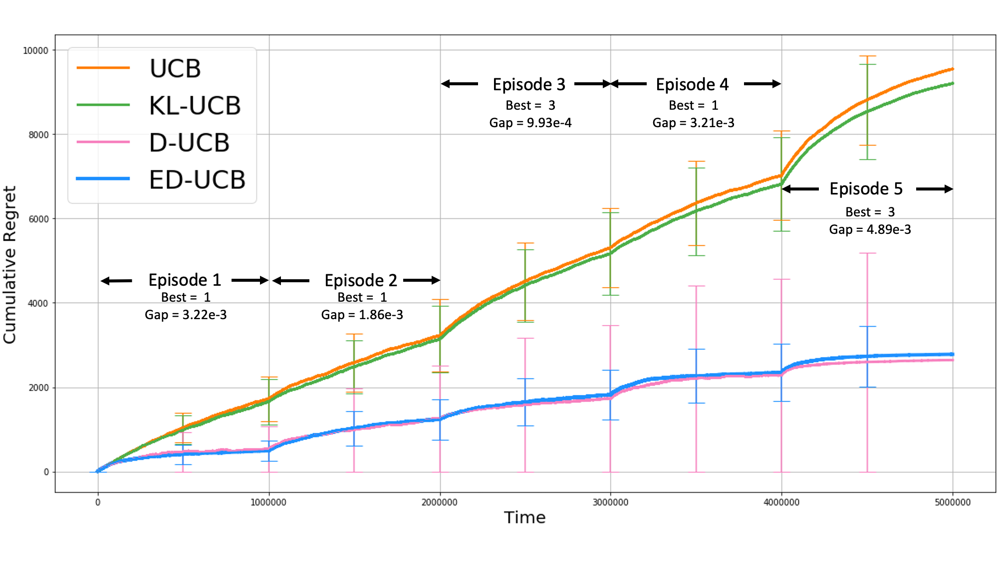
Figure 1: Experiments on the Movielens 1M data set: An experiment with 5 episodes with $10^{6}$ steps each. Plots are averaged over 100 independent runs, error bars indicate one standard deviation. Indices of the best expert and the minimum suboptimality gaps are presented. ED-UCB easily outperforms the naive UCB, KL-UCB algorithms and performs comparably to D-UCB, which is given full knowledge.

5.3 Remarks and Open Questions

1. Lack of lower bound $p_{V}$: Our assumption of the knowledge of $p_{V}$ allows us to develop IS estimates that are finite, leading to constant regret. If there exist a sub-optimal expert that does not satisfy this bound, it would have to be explored at a logarithmic rate since there is no information leakage with respect to this expert. However, samples could still be shared among the other experts through the use of ED-UCB, making it a stronger baseline than naive policies. The question of optimality in this case remains open.

2. Infinite context spaces: The context distribution $p_{e}(x)$ has only been used the quantities $M_{ij,e}$ and the upper bound $M$ (Equation 1). For continuous contexts, the results in Section 4 can be extended by assuming knowledge of upper and lower bounds on the density function $p_{e}(x)$ and swapping out the summation for an integral in Equation (1). This can further be extended to the episodic case by assuming access to approximate oracles for expert policies.

3. Stochastic episode lengths and unknown change-points: Our analysis extends to the setting where the number of episodes and the length of each episode are random quantities with upper bounds $E,T$ respectively. In the case where the end of the episode is not communicated to the agent, ED-UCB can potentially be slow to adapt to the modified environment which leads to linear regret. Thus, tracking the best expert in unknown non-stationary environments is an important avenue for future work.

6 Experiments

We now present numerical experiments to validate our results above. We use the Movielens 1M data set [Harper and Konstan, 2015] with 1 million ratings of approximately 3900 movies by 6000 users to construct a semi-synthetic bandit instance. First, we complete the reward matrix (scaled down to $(0,1)$) using the SoftImpute algorithm of [Mazumder et al., 2010] included in the fancyimpute package [Rubinsteyn and Feldman, 2016]. We filter the number of movies to 618 using the completed matrix by eliminating ones that are mostly rated 0. Then, we cluster these movies based on 7 genres namely: Action, Children, Comedy, Drama, Horror, Romance, Thriller and users based on ages between $0-17,18-24,25-49,49+$. At this stage, the average reward of all (age,genre) pairs are close to each other. To induce some diversity, we boost the rewards of the following (age,genre) pairs by 0.008: (0-17,Children), (18-24,Horror), (18-24,Thriller), (25-49,Action) and (25-49,Drama).

Experts are then randomly generated over the set of genres randomly with $p_{V}=0.002$. Given an age group (context) and genre (expert-recommended action), a movie of the selected genre is picked uniformly and the reward is obtained from the completed reward matrix. We build empirical expert policies using Theorem 7 with $p_{V}=0.2$ and a prior distribution satisfying $p_{X}=0.05$ for $5$ episodes of length $10^{6}$ each. We compare ED-UCB with D-UCB, UCB and KL-UCB. We set the parameter $C$ used by ED-UCB and D-UCB to 0.02. The averaged results of 100 independent runs are presented in Figure 1.

The mismatch in $p_{V}$ in the sampling process causes the empirical estimates being formed with fewer samples than theoretically recommended. However, we empirically observe that ED-UCB still heavily outperforms the naive bandit policies and is comparable in regret to D-UCB.

7 Conclusions

We study the Episodic Bandit problem with Stochastic Experts and show that the use of clipped Importance Sampling estimators built using approximate knowledge of expert policies can lead to constant average regret which improves heavily over naive bandit policies and is comparable to the performance of the state-of-the-art when the expert policies are known.

Our contributions are mainly algorithmic and analytical. In practice, our methods can be used to recommend products to user populations in an online manner. Here, biases derived from the data in the bootstrapping phase of our methods can prevail in the online phase, leading to insensitive recommendations. Thus, it is important to judge the data being used to build these systems and extensively test them before deployment.

Appendix A Notations

In this section, we summarize definitions and descriptions of all the notation used in the main body of this paper.

A.1 Notations in Section 2

• $\mathcal{X},\mathcal{V}$: These represent the finite sets that the contexts and actions are picked from respectively.

• $\Pi=\{\pi_{1},\pi_{2},...,\pi_{N}\}$: The set of $N$ experts provided to the agent. Expert $\pi_{i}$ is equivalently referred to as expert $i$ for any $i\in[N]$. Each expert $i$ is characterized by $|\mathcal{X}|$ probability distributions over the set $\mathcal{V}$. Specifically, given a context $x\in\mathcal{X}$, the expert $i$ is characterized by the conditional distribution $\pi_{i}(v|x)$ for each $v\in\mathcal{V}$.

• $Y$: The reward variable. It is assumed that $Y\in[0,1]$ but this can be extended to any bounded interval with appropriate shifting and scaling.

• $E,T$: The number of episodes and the length of each episode respectively.

• $p_{e}(\cdot),q_{e}(\cdot|x,v)$: The context and reward distributions at each time in episode $e\in[E]$. Specifically, in episode $e$, for each $t\in[T],$ the context $X_{t,e}\sim p_{e}(\cdot)$, $Y_{t,e}\sim q_{e}(\cdot|X_{t,e},V_{t,e})$ where $V_{t,e}\sim\pi_{i_{t,e}}(\cdot|X_{t,e})$ is the action recommended by the agent $i_{t,e}$ chosen by the agent.

• $\mu_{i,e}$: The mean of expert $i$ in episode $e$. Mathematically, $\mu_{i,e}=\mathbb{E}_{i,e}[Y]$ where the expectation over the joint distribution $p_{e}(\cdot)\pi_{i}(\cdot|\cdot)q_{e}(\cdot|\cdot,\cdot)$.

• $\mu^{*}_{e}$: The mean of the best expert in episode $e$, $\mu^{*}=\max_{i\in[N]}\mu_{i,e}$.

A.2 Notations in Section 3

• $\xi$: The maximum error in the the estimation of the empirical experts provided to the agent. For all $i\in[N]$, the empirical expert policies $\hat{\pi}_{i}$ satisfy

  $$\|\pi_{i}-\hat{\pi}_{i}\|_{\infty}\leq\xi$$

• $p_{V}$: The lower bound on the mass that any expert can levy on any action in the set $\mathcal{V}$, i.e., $\forall v\in\mathcal{V},x\in\mathcal{X},\pi_{i}(v|x)\geq p_{V}>0.$

• $\hat{r}_{ij}(v|x)$: The empirical Importance Sampling (IS) ratio between experts $i,j$ on the action $v$ under context $x$, $\hat{r}_{ij}(v|x)=\frac{\pi_{i}(v|x)}{\pi_{j}(v|x)}$.

• $\underline{r}_{ij},\overline{r}_{ij}$: Upper and lower confidence bounds on the estimated IS ratio $\hat{r}_{ij}$. Specifically,

  $$\underline{r}_{ij}(v|x) =\hat{r}_{ij}(v|x)-\frac{\xi}{p_{V}(p_{V}-\xi)}$$

  $$\overline{r}_{ij}(v|x) =\hat{r}_{ij}(v|x)+\frac{\xi}{p_{V}(p_{V}+\xi)}.$$

• $\underline{D}_{f_{1}}(i||j),\underline{M}_{ij}$: Estimates of the $f_{1}$-divergence between the experts $i$ and $j$. Here, $f_{1}(x)=x\exp(x-1)-1$.

  $$\underline{D}_{f_{1}}(i||j)=p_{X}\sum_{x\in\mathcal{X}}\sum_{v\in\mathcal{V}}\left(\hat{\pi}_{i}(v|x)-\xi\right)f_{1}\left(\underline{r}_{ij}(v|x)\right)~{}~{}~{},~{}~{}~{}\underline{M}_{ij}=1+\log(1+\underline{D}_{f_{1}}(i||j))$$

• $p_{X}$: The lower bound on the probability of occurrence of the least frequent context, i.e., $\forall x\in\mathcal{X},e\in[E],p_{e}(x)\geq p_{X}>0.$

• $Z_{i}(t)$: The normalizing factor in the IS sampling estimator. $Z_{i}(t)=\sum_{s=1}^{t}\underline{M}_{ik_{t}}$ for each expert $i$ where $k_{s}$ is the expert picked at time $s$.

• $\epsilon_{i}(t)$: The bias of the IS sampling estimator due to clipping. For this, we define $w(x)=y\iff\frac{y}{\log\left(\frac{2}{y}\right)}=x$. Then, $\epsilon_{i}(t)=Cw\left(\frac{\sqrt{t\log t}}{Z_{i}(t)}\right).$

• $\tilde{Y}_{i}(t)$: The IS estimate of the mean of expert $i$ by time $t$.

  $$\tilde{Y}_{i}(t)=\frac{1}{Z_{i}(t)}\sum_{s=1}^{t}\frac{Y_{s}}{\underline{M}_{ik_{s}}}\underline{r}_{ik_{s}}\mathbbm{1}\left\{\overline{r}_{ik_{s}}\leq 2\log\left(\frac{2}{\epsilon_{i}(t)}\right)\underline{M}_{ik_{s}}\right\}.$$

• $e_{i}(t)$: The maximum error in the IS estimate due to use of estimated quantities. Specifically,

  $$e_{i}(t)=\max_{x\in\mathcal{X},v\in\mathcal{V},j\in[N]}\overline{r}_{ij}(v|x)-\underline{r}_{ij}(v|x)\mathbbm{1}\left\{\overline{r}_{ij}(v|x)\leq 2\frac{2}{\epsilon_{i}(t)}\underline{M}_{ij}\right\}.$$

• $U_{i}(t)$: The Upper Confidence Bound estimate of the mean of expert $i$ that includes the IS estimate, the total bias due to clipping and estimation. $U_{i}(t)=\tilde{Y}_{i}(t)+\frac{3}{2}\epsilon_{i}(t)+e_{i}(t).$

Notation in Section 4:

• $D_{f_{1}}(i||j),M_{ij}$: The true divergence between experts $i,j$ given by

  $$D_{f_{1}}(i||j)=\sum_{x\in\mathcal{X}}p(x)\sum_{v\in\mathcal{V}}\pi_{i}(v|x)f_{1}\left(\frac{\pi_{i}(v|x)}{\pi_{j}(v|x)}\right)~{}~{}~{},~{}~{}~{}M_{ij}=1+\log(1+D_{f_{1}}(i||j))$$

• $M$: The upper bound on the true maximum divergence between any two experts $i,j$, $M\geq\max_{i,j\in[N]}M_{ij}$. A trivial upper bound is used, given by $M=(1-p_{X})|\mathcal{X}||\mathcal{V}|f_{1}\left(\frac{p_{V}}{1-p_{V}}\right)$. We also set $C=\frac{32M}{\gamma(1-p_{V})}$ for analysis.

• $\gamma$: The lower bound on the mean reward of any expert over all episodes, $\mu_{i,e}\geq\gamma>0.$

• $\mathbf{\Delta}$: The vector of suboptimality gaps, $\mathbf{\Delta}=(\Delta_{1},\Delta_{2},...,\Delta_{N})$ where $\Delta_{i}=\mu^{*}-\mu_{i}$. We assume here that without loss of generality, experts are arranged in decreasing order of means: $\mu^{*}=\mu_{1}>\mu_{2}\geq\mu_{3}\geq...\geq\mu_{N}$.

• $T_{clip}$: The first time at which all clippers are active for all experts, i.e.,

  $$T_{clip}=\min\{t:\forall v\in\mathcal{V},x\in\mathcal{X},i,j\in[N],\overline{r}_{ij}(v|x)\leq 2\log\left(2/\epsilon_{i}(t)\right)\underline{M}_{ij}\}.$$

• $T_{1}$: The first time at which one can conclude with high probability that the best arm is never underestimated. We define

  $$\tau_{1} =\min\left\{t:Cw\left(\sqrt{\log t/t}\right)\leq\gamma\right\}$$

  $$T_{1} =\max\{\tau_{1},T_{clip}\}.$$

  For any $t\geq T_{1},$ with probability at least $1-t^{-2}$, $U_{1}(t)\geq\mu^{*}.$

• $T_{i}$: The first time at which one can conclude with high probability that the $i^{th}$-best expert is never overestimated. We define

  $$\tau_{i} =\min\left\{t:\frac{t}{\log t}\geq\frac{9C^{2}M^{2}\log^{2}\left(\frac{6C}{(\Delta_{i}-\gamma p_{V})}\right)}{\left(\Delta_{i}-\gamma p_{V}\right)^{2}}\right\}$$

  $$T_{i} =\max\{T_{1},\tau_{i}\}.$$

  For any $t\geq T_{i}$, with probability at least $1-t^{-2}$, $U_{i}(t)\leq\mu^{*}$.

• $R(T)$: The regret suffered by the agent by time $T$, $R(T)=\sum_{t=1}^{T}\mu^{*}-\mu_{k_{t}}$.

Appendix B Some Useful Concentrations

We start with some useful concentration inequalities. First we consider a modified result from [Weissman et al., 2003]:

Lemma 8.

Let $p$ be a probability vector with $S$ points of support. Let $\hat{p}\sim\frac{1}{n}Multinomial(n,p)$ be an empirical estimate of $p$ using $n$ i.i.d. draws. Then, for any $S\geq 2$ and $\delta\in(0,1)$, it holds that

$$\mathbb{P}\left(\|p-\hat{p}\|_{\infty}\geq\sqrt{\frac{2S\log\left(\frac{2}{\delta}\right)}{n}}\right)\leq\mathbb{P}\left(\|p-\hat{p}\|_{1}\geq\sqrt{\frac{2S\log\left(\frac{2}{\delta}\right)}{n}}\right)\leq\delta$$

Proof: The result follows from that of [Weissman et al., 2003] as $\|x\|_{\infty}\leq\|x\|_{1}$ for any vector $x$. $\hfill\square$

The next lemma is a adapted from the Lemma 5.1 in [Cayci et al., 2019]. It provides confidence bounds for ratios of random variables.

Lemma 9.

Suppose $\pi_{i},\pi_{j}$ are probability vectors that share the same support $\mathcal{S}$ with at least mass $c$ on each support point. Let $\hat{\pi}_{i},\hat{\pi}_{j}$ be their respective empirical estimates such that $\mathbb{P}\left(\|\pi_{i}-\hat{\pi}_{i}\|_{\infty}>\xi\right)\leq\delta$. Call, for each $s\in\mathcal{S}$, $\nicefrac{{\pi_{i}(s)}}{{\pi_{j}(s)}}=r_{ij}(s)$ and $\nicefrac{{\hat{\pi}_{i}(s)}}{{\hat{\pi}_{j}(s)}}=\hat{r}_{ij}(s)$. With probability at least $1-\delta$, it holds that

$$r_{ij}(s)\in\left[\hat{r}_{ij}(s)-\frac{\xi}{c(c-\xi)},\hat{r}_{ij}(s)+\frac{\xi}{c(c+\xi)}\right]~{}~{}~{}~{}\forall s\in\mathcal{S}$$

Proof: The proof follows the result from of Lemma 5.1 in [Cayci et al., 2019]. To ease notation, we fix an arbitrary $s\in\mathcal{S}$ and denote $\mu_{k}=\pi_{k}(s)$, $X_{k}=\hat{\pi}_{k}(s)$ for $k\in\{i,j\}$. Under the event that $\|\mu_{k}-X_{k}\|_{\infty}\leq\xi$ for $k\in\{i,j\}$, we have

$$\frac{X_{i}}{X_{j}} \geq\frac{\mu_{i}-\xi}{\mu_{j}+\xi}$$

$$=\frac{\mu_{i}-\xi}{\mu_{j}+\xi}\times\frac{\mu_{j}}{\mu_{j}}$$

$$=\frac{\mu_{j}\mu_{i}-\mu_{j}\xi+\mu_{i}\xi-\mu_{i}\xi}{\mu_{j}(\mu_{j}+\xi)}$$

$$=\frac{\mu_{i}(\mu_{j}+\xi)-\xi(\mu_{i}+\mu_{j})}{\mu_{j}(\mu_{j}+\xi)}$$

$$=\frac{\mu_{i}}{\mu_{j}}-\frac{\xi}{\mu_{j}+\xi}\left(1+\frac{\mu_{i}}{\mu_{j}}\right)$$

$$\geq\frac{\mu_{i}}{\mu_{j}}-\frac{\xi}{c+\xi}\left(1+\frac{1-c}{c}\right)$$

$$=\frac{\mu_{i}}{\mu_{j}}-\frac{\xi}{c(c+\xi)}.$$

Similarly, we have that

$$\frac{X_{i}}{X_{j}} \leq\frac{\mu_{i}+\xi}{\mu_{j}-\xi}$$

$$\leq\frac{\mu_{i}}{\mu_{j}}+\frac{\xi}{c(c-\xi)}.$$

Since the choice of $s\in\mathcal{S}$ was arbitrary and the event $\|\mu_{k}-X_{k}\|_{\infty}\leq\xi$ holds with probability at least $1-\delta$, the result follows.$\hfill\square$

Appendix C Proofs of results in Section 4

To prove the concentration result in Theorem 2, we will first consider a simpler setting of two arms with deterministic samples. We refer the reader to Section A for definitions and descriptions of quantities used here.

C.1 A simpler case of two arms

We begin by considering 2 arms, $i,j$. We are given access to $t$ samples from arm $j$ and seek to estimate the mean of arm $i$ using the approximate experts $\hat{\pi}_{i},\hat{\pi}_{j}$ with maximum error $\xi$. The arguments in this section closely follow the analysis of the two armed estimator in the full information case in [Sen et al., 2017]. We start with the following assumption:

Assumption 1.

$\xi$ is such that

$$\frac{\xi}{p_{V}}\left(\frac{1}{(p_{V}-\xi)}+\frac{1}{(p_{V}+\xi)}\right)=\frac{\gamma p_{V}}{2}$$

We define

$$\underline{r}_{ij}(v|x) =\hat{r}_{ij}(v|x)-\frac{\xi}{p_{V}(p_{V}-\xi)}$$

$$\overline{r}_{ij}(v|x) =\hat{r}_{ij}(v|x)+\frac{\xi}{p_{V}(p_{V}+\xi)}.$$

Note that by Lemma 9, we have that

$$\underline{r}_{ij}(v|x)\leq\hat{r}_{ij}(v|x)\leq\overline{r}_{ij}(v|x).$$

For an arbitrarily chosen $\epsilon\in(0,1)$, we write

$$\eta^{\prime} :=\min\left\{a:\mathbb{P}_{i}\left(\underline{r}_{ij}>a\right)\leq\frac{\epsilon}{2}\right\}.$$ (4)

Then, we have the following claims:

Claim 1.

With $\eta,\eta^{\prime}$ as above, for any $\epsilon\in(0,1),$ we have that $\eta^{\prime}\leq\eta$.

Proof: Since $\underline{r}_{ij}\leq r_{ij}$, for any $a$, we have that $\mathbb{P}_{i}(\underline{r}_{ij}>a)\leq\mathbb{P}_{i}(r_{ij}>a).$ Let $A_{1}=\{a:\mathbb{P}_{i}(\underline{r}_{ij}>a)\leq\epsilon/2\}$ and $A_{2}=\{a:\mathbb{P}_{i}(r_{ij}>a)\leq\epsilon/2\}$. For any $a\in A_{2}$, it must be that $a\in A_{1}$. Thus, $A_{2}\subseteq A_{1}$. Therefore, $\min A_{2}\geq\min A_{1}$. By recalling the definitions of $\eta,\eta^{\prime}$, we have $\eta^{\prime}\leq\eta$. $\square$

Claim 2.

For any $\epsilon\in(0,1)$, we have that $\mathbbm{1}\{r_{ij}\leq\eta\}\geq\mathbbm{1}\{\overline{r}_{ij}\leq\eta^{\prime}\}.$

Proof: Since $r_{ij}\leq\overline{r}_{ij}$, we have that, $\mathbbm{1}\{\overline{r}_{ij}\leq\eta^{\prime}\}\leq\mathbbm{1}\{{r}_{ij}\leq\eta^{\prime}\}$. Further, since $\eta^{\prime}\leq\eta$ from Claim 1, we have that $\mathbbm{1}\{{r}_{ij}\leq\eta^{\prime}\}\leq\mathbbm{1}\{{r}_{ij}\leq\eta\}$. Combining the above, we obtain the result. $\square$

Our estimator for $\mu_{i}$ based on $t$ samples from expert $j$ is then defined as

$$\tilde{Y}_{i}(j,t)=\frac{1}{t}\sum_{s=1}^{t}Y_{s}\underline{r}_{ij}(s)\mathbbm{1}\left\{\overline{r}_{ij}(s)\leq\eta^{\prime}\right\}.$$ (5)

We recall the corresponding IS estimate with full information in the following lemma

Lemma 10.

Define $\eta:=\min\left\{a:\mathbb{P}_{i}\left(\frac{\pi_{i}(V|X)}{\pi_{j}(V|X)}>a\right)\leq\frac{\epsilon}{2}\right\}$ and the full information IS estimator as

$$\hat{Y}_{i}^{\eta}(j,t):=\frac{1}{t}\sum_{s=1}^{t}Y_{s}\frac{\pi_{i}(V_{s}|X_{s})}{\pi_{j}(V_{s}|X_{s})}\mathbbm{1}\left\{\frac{\pi_{i}(V_{s}|X_{s})}{\pi_{j}(V_{s}|X_{s})}\leq\eta\right\}$$ (6)

Then, for all $t\geq 1$, it holds that $\mathbb{E}_{j}[\hat{Y}_{i}^{\eta}(j,t)]\leq\mu_{i}\leq\mathbb{E}_{j}[\hat{Y}_{i}^{\eta}(j,t)]+\frac{\epsilon}{2}$.

We now compare our estimator in Equation 5 to the full information estimator in Equation 6. Due to Claim 2, it holds trivially that

$$\tilde{Y}_{i}(j,t)\leq\hat{Y}_{i}(j,t).$$

Consider the following chain:

$$\hat{Y}_{i}(j,t) =\frac{1}{t}\sum_{s=1}^{t}Y_{s}r_{ij}(s)\mathbbm{1}\{r_{ij}(s)\leq\eta\}+\tilde{Y}_{i}(j,t)-\tilde{Y}_{i}(j,t)$$

$$=\tilde{Y}_{i}(j,t)+\frac{1}{t}\sum_{s=1}^{t}Y_{s}\left(r_{ij}(s)\mathbbm{1}\{r_{ij}(s)\leq\eta\}-\underline{r}_{ij}(s)\mathbbm{1}\{\overline{r}_{ij}(s)\leq\eta^{\prime}\}\right)$$

$$\leq\tilde{Y}_{i}(j,t)+\frac{1}{t}\sum_{s=1}^{t}Y_{s}\left(\overline{r}_{ij}(s)-\underline{r}_{ij}(s)\mathbbm{1}\{\overline{r}_{ij}(s)\leq\eta^{\prime}\}\right)$$

$$\leq\tilde{Y}_{i}(j,t)+\frac{1}{t}\sum_{s=1}^{t}\left(\overline{r}_{ij}(s)-\underline{r}_{ij}(s)\mathbbm{1}\{\overline{r}_{ij}(s)\leq\eta^{\prime}\}\right)$$

$$\leq\tilde{Y}_{i}(j,t)+e_{ij}$$

Here, the second inequality holds since $e_{ij}:=\max_{v,x}\overline{r}_{ij}-\underline{r}_{ij}\mathbbm{1}\{\overline{r}_{ij}\leq\eta^{\prime}\}\geq 0$ and $Y_{s}\leq 1$. As a result of the arguments above, we have the following Lemma:

Lemma 11.

With $\hat{Y}_{i}(j,t)$ and $\tilde{Y}_{i}(j,t)$ as defined in Equations 6 and 5 respectively and $e_{ij}:=\max_{v,x}\overline{r}_{ij}-\underline{r}_{ij}\mathbbm{1}\{\overline{r}_{ij}\leq\eta^{\prime}\}$, it holds that

$$\mathbb{E}_{j}[\tilde{Y}_{i}(j,t)]\leq\mathbb{E}_{j}[\hat{Y}_{i}(j,t)]\leq\mathbb{E}_{j}[\tilde{Y}_{i}(j,t)]+e_{ij}.$$

As a result of Lemma 10, we thus have the following corollary:

Corollary 11.1.

The mean of the estimator $\tilde{Y}_{i}(j,t)$ according to the distribution of arm $j$ satisfies

$$\mathbb{E}_{j}[\tilde{Y}_{i}(j,t)]\in\left[\mu_{i}-\frac{\epsilon}{2}-e_{ij},\mu_{i}\right]$$ (7)

C.1.1 Simpler clipper levels

In this section, we move from the abstract clipper levels $\eta^{\prime}$ to those based on divergences as in the estimator used in ED-UCB. To this end, using Markov’s inequality, we have

$$\mathbb{P}_{i}(\underline{r}_{ij}>a)\leq\exp(-a)\mathbb{E}_{i}[\exp(\underline{r}_{ij})]$$

Suppose that the RHS of the above is upper bounded by $\frac{\epsilon}{2}$. That is, $\exp(a)\geq\frac{2}{\epsilon}\mathbb{E}_{i}[\underline{(}r_{ij})]$. Consider the following chain:

$$\mathbb{E}_{i}[\exp(\underline{r}_{ij})] =e+e\left(\mathbb{E}_{i}[\exp(\underline{r}_{ij}-1)]-1\right)$$

$$=e+e\left(\mathbb{E}_{j}[r_{ij}\exp(\underline{r}_{ij}-1)-1]\right)$$

$$\geq e+e\left(\mathbb{E}_{j}[\underline{r}_{ij}\exp(\underline{r}_{ij}-1)-1]\right)$$

$$=e+e\underline{D}_{f_{1}}(\pi_{i}||\pi_{j})$$

Therefore, the RHS of the Markov inequality is upper bounded by $\frac{\epsilon}{2}$ if $\exp(a)\geq\frac{2}{\epsilon}(e+e\underline{D}_{f_{1}}(\pi_{i}||\pi_{j}))$ or, equivalently, if $a\geq\log\left(\frac{2}{\epsilon}\right)+\underline{M}_{ij}$. However, by definition, we must have that $\eta^{\prime}\leq\log\left(\frac{2}{\epsilon}\right)+\underline{M}_{ij}\leq 2\log\left(\frac{2}{\epsilon}\right)\underline{M}_{ij}$.

Therefore, we redefine our original estimator in Equation 5 to use this new clipper level $\alpha_{i}(j,\epsilon):=2\log\left(\frac{2}{\epsilon}\right)\underline{M}_{ij}$. We have

$$\tilde{Y}_{i}(j,t):=\frac{1}{t}\sum_{s=1}^{t}Y_{s}\underline{r}_{ij}(s)\mathbbm{1}\{\overline{r}_{ij}(s)\leq\alpha_{i}(j,\epsilon)\}$$ (8)

We also restate Lemma 11 for convenience:

Lemma 12.

For $\tilde{Y}_{i}(j,t)$ defined as above, and $e_{ij}=\max_{v,x}\overline{r}_{ij}-\underline{r}_{ij}\mathbbm{1}\{\overline{r}_{ij}\leq\alpha_{i}(j,\epsilon)\}$,

$$\mathbb{E}_{j}[\tilde{Y}_{i}(j,t)]\in\left[\mu_{i}-\frac{\epsilon}{2}-e_{ij},\mu_{i}\right]$$ (9)

C.2 Proof of Theorem 2

Now, we consider the setting as in Section 3. Recall the clipped IS estimator defined as

$$\tilde{Y}_{i}(t):=\frac{1}{\sum_{s=1}^{t}\left(\frac{1}{\underline{M}_{ik_{s}}}\right)}\sum_{s=1}^{t}\frac{Y_{s}}{\underline{M}_{ik_{s}}}\underline{r}_{ik_{s}}(s)\mathbbm{1}\{\overline{r}_{ik_{s}}(s)\leq\alpha_{i}(k_{s},s)\}.$$ (10)

To provide concentrations for the above estimator, we define the following filtration by time $t$: $\mathcal{F}_{t}=\sigma\left(\{k_{s},X_{s},V_{s},Y_{s}\}_{s=1}^{t-1},k_{t}\right)$. Note that the filtration at time $t$ contains information about all the observations upto time $t-1$ as well as the choice of the arm at time $t$. We now define the following martingale that will be used to analyze the estimator:

$$A_{0} :=0$$

$$A_{s} :=\sum_{l=1}^{s}\frac{L_{i}(l)}{\underline{M}_{ik_{l}}}-\sum_{l=1}^{s}\mathbb{E}\left[\frac{L_{i}(l)}{\underline{M}_{ik_{l}}}\Big{|}\mathcal{F}_{l-1}\right]$$

Where, to ease notation, we write $L_{i}(l)=Y_{l}\underline{r}_{ik_{l}}(l)\mathbbm{1}\{\overline{r}_{ik_{l}}(l)\leq\alpha_{i}(k_{l},l)\}$. Since $\mathcal{F}_{l-1}$ contains knowledge of $k_{l}$, the second term in $A_{s}$ can be further simplified using $\mu_{i}(l)=\mathbb{E}[L_{i}(l)|\mathcal{F}_{l-1}]$ as

$$A_{s}=\sum_{l=1}^{s}\frac{L_{i}(l)}{\underline{M}_{ik_{l}}}-\sum_{l=1}^{s}\frac{\mu_{i}(l)}{\underline{M}_{ik_{l}}}$$

Remark 13.

Using Lemma 12, we can write that $\mu_{i}(l)\in\left[\mu_{i}-\frac{\epsilon}{2}-e_{i}(t),\mu_{i}\right]$ where $e_{i}(t):=\max_{j}e_{ij}$.

It is easy to see that $|A_{s}-A_{s-1}|\leq 4\log\left(\frac{2}{\epsilon}\right)$. Therefore, using the Azuma-Hoeffding inequality for martingales with bounded differences, we can write:

$$\mathbb{P}\left(\Big{|}\sum_{l=1}^{t}\frac{L_{i}(l)}{\underline{M}_{ik_{l}}}-\sum_{l=1}^{t}\frac{\mu_{i}(l)}{\underline{M}_{ik_{l}}}\Big{|}\geq\beta\right)\leq 2\exp\left(-\frac{\beta^{2}}{32t\log^{2}\left(\frac{2}{\epsilon}\right)}\right)$$

We are now ready to begin the proof of our concentration result.

Proof (Proof of Theorem 2): We assess the two tail bounds of the Azuma-Hoeffding inequality separately.

1. Upper tail:
For any $\beta(t)>0$, we have the following chain:

$$(1+\beta(t))\left(\max_{l\in[t]}\mu_{i}(l)\right)\sum_{l=1}^{t}\frac{1}{\underline{M}_{ik_{l}}} \geq\sum_{l=1}^{t}\frac{\mu_{i}(l)}{\underline{M}_{ik_{l}}}+\frac{t}{M}\times\beta(t)\times\max_{l\in[t]}\mu_{i}(l)$$

$$\geq\sum_{l=1}^{t}\frac{\mu_{i}(l)}{\underline{M}_{ik_{l}}}+\frac{\beta(t)t}{M}\left(\frac{\gamma}{2}-e_{i}(t)\right)$$

The final inequality uses Remark 13 with $\epsilon(t)\leq\gamma\leq\mu_{i}$ for all $i\in\mathcal{A}$. Thus, we have that

$$\mathbb{P}\left(\tilde{Y}_{i}(t)\geq(1+\beta(t))(\max_{l\in[t]}\mu_{i}(l)\right) \leq\mathbb{P}\left(\sum_{l=1}^{t}\frac{L_{i}(l)}{\underline{M}_{ik_{l}}}\geq\sum_{l=1}^{t}\frac{\mu_{i}(l)}{\underline{M}_{ik_{l}}}+\frac{\beta(t)t}{M}\left(\frac{\gamma}{2}-e_{i}(t)\right)\right)$$

$$\leq\exp\left(-\frac{t\beta^{2}(t)\left(\frac{\gamma}{2}-e_{i}(t)\right)^{2}}{32M^{2}\log^{2}\left(\frac{2}{\epsilon(t)}\right)}\right).$$

2. Lower Tail:
Analogous to the arguments for the upper tail, we have that

$$(1-\beta(t))\left(\min_{l\in[t]}\mu_{i}(l)\right)\sum_{l=1}^{t}\frac{1}{\underline{M}_{ik_{l}}}\leq\sum_{l=1}^{t}\frac{\mu_{i}(l)}{\underline{M}_{ik_{l}}}-\frac{\beta(t)t}{M}\left(\frac{\gamma}{2}-e_{i}(t)\right).$$

Therefore, we have that

$$\mathbb{P}\left(\tilde{Y}_{i}(t)\leq(1-\beta(t))(\min_{l\in[t]}\mu_{i}(l))\right) \leq\mathbb{P}\left(\sum_{l=1}^{t}\frac{L_{i}(l)}{\underline{M}_{ik_{l}}}\leq\sum_{l=1}^{t}\frac{\mu_{i}(l)}{\underline{M}_{ik_{l}}}-\frac{\beta(t)t}{M}\left(\frac{\gamma}{2}-e_{i}(t)\right)\right)$$

$$\leq\exp\left(-\frac{t\beta^{2}(t)\left(\frac{\gamma}{2}-e_{i}(t)\right)^{2}}{32M^{2}\log^{2}\left(\frac{2}{\epsilon(t)}\right)}\right).$$

Combining the two tails with Remark 13, we get

$$\mathbb{P}\left(\tilde{Y}_{i}(t)\not\in\left[(1-\beta(t))\left(\mu_{i}-\frac{\epsilon(t)}{2}-e_{i}(t)\right),(1+\beta(t))\mu_{i}\right]\right)$$

$$\hfill\leq 2\exp\left(-\frac{t\beta^{2}(t)\left(\frac{\gamma}{2}-e_{i}(t)\right)^{2}}{32M^{2}\log^{2}\left(\frac{2}{\epsilon(t)}\right)}\right).$$

$\square$

C.3 Per-expert concentrations

In this section, we provide concentration results for optimal and sub-optimal experts separately. We begin with the following claim:

Claim 3.

For all $t\geq T_{clip}$ and all $k\in[N]$, $e_{k}(t)=\frac{\gamma p_{V}}{2}$.

Proof: Fix $i,j\in[N]$ and $(v,x)\in\mathcal{V}\times\mathcal{X}$, arbitrary. Consider at some $t\geq T_{clip}$

$$\overline{r}_{ij}(v|x)-\underline{r}_{ij}(v|x)\mathbbm{1}\left\{\overline{r}_{ij}(v|x)\leq\alpha_{ij}(t)\right\}$$

$$= \overline{r}_{ij}(v|x)-\underline{r}_{ij}(v|x)~{}~{}~{}~{}~{}(\text{By definition of $T_{clip}$})$$

$$= \frac{\xi}{p_{V}}\left(\frac{1}{(p_{V}-\xi)}+\frac{1}{(p_{V}+\xi)}\right)$$

$$= \frac{\gamma p_{V}}{2}~{}~{}~{}~{}(\text{By Assumption \ref{asm: confidence for ratio}})$$

Since this holds for the arbitrary choice of $i,j,v,x$, it must hold that

$$e_{k}(t) =\max_{j,v,x}\overline{r}_{kj}(v|x)-\underline{r}_{kj}(v|x)\mathbbm{1}\left\{\overline{r}_{kj}(v|x)\leq\alpha_{kj}(t)\right\}$$

$$=\frac{\gamma p_{V}}{2}.$$

$\square$

The following lemma provides concentrations for the best arm:

Lemma 14.

Let $\beta_{k^{*}}^{\prime}(t)=Cw\left(\sqrt{\frac{\log t}{t}}\right)$ and define $\tau_{1}=\min\{t:\beta_{k^{*}}^{\prime}(t)\leq\gamma\}$, $T_{1}=\max\{\tau_{1},T_{clip}\}$. Then, for all $t\geq T_{1}$, it holds that

$$\mathbb{P}(U_{k^{*}}(t)\leq\mu^{*})\leq\frac{1}{t^{2}}.$$

Proof: We have that for $t\geq T_{1},$

$$\mathbb{P}(U_{k^{*}}\leq\mu^{*}) =\mathbb{P}\left(\tilde{Y}_{k^{*}}(t)\leq\mu^{*}-\frac{3}{2}\beta_{k^{*}}(t)-e_{k^{*}}\right)$$

$$\leq\mathbb{P}\left(\tilde{Y}_{k^{*}}(t)\leq\mu^{*}-\frac{3}{2}\beta^{\prime}_{k^{*}}(t)-e_{k^{*}}\right)$$

$$~{}~{}~{}~{}~{}~{}~{}~{}~{}~{}~{}~{}\left(Z_{k}^{*}(t)\leq t,w(x)\text{ increasing}\implies\beta_{k^{*}}(t)\geq\beta^{\prime}_{k^{*}}(t)\right)$$

$$\leq\mathbb{P}\left(\tilde{Y}_{k^{*}}(t)\leq\mu^{*}-\mu^{*}\beta^{\prime}_{k^{*}}(t)-(1-\beta^{\prime}_{k^{*}}(t))\left(\frac{\beta^{\prime}_{k^{*}}(t)}{2}+e_{k^{*}}\right)\right)$$

$$~{}~{}~{}~{}~{}~{}~{}~{}~{}~{}~{}~{}\left(\beta^{\prime}_{k^{*}}(t)\leq\gamma\leq\mu^{*}\leq 1\text{ for }t\geq T_{1}\right)$$

$$=\mathbb{P}\left(\tilde{Y}_{k^{*}}(t)\leq(1-\beta^{\prime}_{k^{*}}(t))\left(\mu^{*}-\frac{\beta^{\prime}_{k^{*}}(t)}{2}-e_{k^{*}}\right)\right).$$

Now, we can apply Theorem 2 with $\epsilon(t)=\beta(t)=\beta^{\prime}_{k^{*}}(t)$. This choice is valid for $\epsilon(t)$ due to the definition of $T_{1}$. Thus, we can write that

$$\mathbb{P}(U_{k^{*}}(t)\leq\mu^{*}) \leq\exp\left(-\frac{\beta^{\prime}_{k^{*}}(t)^{2}t\left(\frac{\gamma}{2}-e_{k^{*}}\right)^{2}}{32M^{2}\log^{2}\left(\frac{2}{\beta^{\prime}_{k^{*}}(t)}\right)}\right)$$

$$=\exp\left(-\frac{\beta^{\prime}_{k^{*}}(t)^{2}t\gamma^{2}\left(1-p_{V}\right)^{2}}{128M^{2}\log^{2}\left(\frac{2}{\beta^{\prime}_{k^{*}}(t)}\right)}\right)$$

Where the equality follows from Claim 3, since $T_{1}\geq T_{clip}$. Consider the exponent:

$$\frac{\beta^{\prime}_{k^{*}}(t)t\gamma^{2}(1-p_{V})^{2}}{128M^{2}\log^{2}\left(\frac{2}{\beta^{\prime}_{k^{*}}(t)}\right)^{2}} =\frac{t\gamma^{2}(1-p_{V})^{2}}{128M^{2}}C^{2}\left(\frac{w\left(\sqrt{\nicefrac{{\log t}}{{t}}}\right)}{\log\left(\nicefrac{{2}}{{Cw\left(\sqrt{\frac{\log t}{t}}\right)}}\right)}\right)^{2}$$

$$\geq 2\log t$$

The final inequality holds for the choice of $C=\frac{32M}{\gamma(1-p_{V})}$ and because $\frac{w(x)}{\log\left(\nicefrac{{2}}{{aw(x)}}\right)}\geq x$ for $a\geq 1$, as is the case with $C$.

Using this bound on the exponent, we arrive at the required result. $\square$

Now, we prove similar results for the suboptimal arms.

Lemma 15.

Define $\tau_{k}=\min\left\{t:\frac{t}{\log t}\geq\frac{9C^{2}M^{2}\log^{2}\left(\nicefrac{{6C}}{{(\Delta_{k}-\gamma p_{V})}}\right)}{(\Delta_{k}-\gamma p_{V})^{2}}\right\}$ and $T_{k}=\max\{T_{1},\tau_{k}\}$ for all $k\neq k^{*}$. Then, for all $t\geq T_{k}$ and $k\neq k^{*}$,

$$\mathbb{P}(U_{k}>\mu^{*})\leq\frac{1}{t^{2}}.$$

Proof: Note that $Z_{k}(t)\geq\frac{t}{M}$. Since $w(x)$ is increasing in $x$, using $t\geq T_{k}$, we can write

$$\frac{3}{2}\beta_{k}(t)+e_{k}(t) =\frac{3C}{2}w\left(\frac{\sqrt{t\log t}}{Z_{k}(t)}\right)+\frac{\gamma p_{V}}{2}$$

$$\leq\frac{3C}{2}w\left(\frac{M\sqrt{t\log t}}{t}\right)+\frac{\gamma p_{V}}{2}$$

$$=\frac{3C}{2}w\left(M\sqrt{\frac{\log t}{t}}\right)+\frac{\gamma c}{2}$$

$$\leq\frac{3C}{2}w\left(\frac{\nicefrac{{(\Delta_{k}-\gamma p_{V})}}{{3C}}}{\log\left(\frac{2}{\nicefrac{{(\Delta_{k}-\gamma p_{V})}}{{3C}}}\right)}\right)+\frac{\gamma p_{V}}{2}$$

$$=\frac{3C}{2}\cdot\frac{\Delta_{k}-\gamma p_{V}}{3C}+\frac{\gamma p_{V}}{2}$$

$$=\frac{\Delta_{k}}{2}$$

Here, the penultimate equality follows from the definition of the $w$ function. Therefore, we can write

$$\mathbb{P}\left(U_{k}(t)>\mu^{*}\right) =\mathbb{P}\left(\tilde{Y}_{k}(t)>\mu^{*}-\frac{3\beta_{k}(t)}{2}-e_{k}(t)\right)$$

$$\leq\mathbb{P}\left(\tilde{Y}_{k}(t)>\mu^{*}-\frac{\Delta_{k}}{2}\right)$$

$$\leq\mathbb{P}\left(\tilde{Y}_{k}(t)>\mu_{k}+\frac{\Delta_{k}}{2}\right)$$

$$\leq\mathbb{P}\left(\tilde{Y}_{k}(t)>\mu_{k}\left(1+\frac{\Delta_{k}}{2}\right)\right)$$

$$\leq\mathbb{P}\left(\tilde{Y}_{k}(t)>\mu_{k}\left(1+\beta^{\prime}_{k}(t)\right)\right)$$

The penultimate inequality uses $\mu_{k}\leq 1$ and the final one follows since $\beta^{\prime}_{k}(t)\leq\beta_{k}(t)\leq\frac{3}{2}\beta(t)_{k}+e_{k}(t)\leq\frac{\Delta_{k}}{2}$. Thus, we can now apply Theorem 2 with $\beta(t)=\epsilon(t)=\beta^{\prime}_{k}(t)$ and follow the exponent bounding arguments as in Lemma 14 to obtain the required result. $\square$

The two lemmas above lead to the following useful corollary:

Corollary 15.1.

For all suboptimal arms $k\neq k^{*}$ and $t\geq T_{k},$ we have that

$$\mathbb{P}(k_{t}=k)\leq\frac{2}{t^{2}}$$

C.4 Main regret result

Now, we are ready to prove our final regret theorem. Note that all the lemmas above are true under the event that $\|\pi_{i}(\cdot|x)-\hat{\pi}(\cdot|x)\|_{\infty}\leq\xi$.

Proof: By definition, we have

$$\mathbb{E}[R(T)] =\sum_{t=1}^{T}\mathbb{E}[\Delta_{k_{t}}]$$

$$=\sum_{t=1}^{T}\sum_{k=2}^{N}\Delta_{k}\mathbb{P}(k_{t}=k).$$

Since the condition on $\xi$ is guaranteed by Assumption 1, using Corollary 15.1, we can write this as

$$\mathbb{E}[R(T)] =\sum_{t=1}^{T}\sum_{k=2}^{N}\Delta_{k}\mathbb{P}(k_{t}=k)$$

$$\leq\sum_{t=1}^{T_{N}-1}\Delta_{N}+\sum_{t=T_{N}}^{T}\Delta_{N}\mathbb{P}(k_{t}=N)+\sum_{t=T_{N}}^{T}\sum_{k=2}^{N-1}\Delta_{k}\mathbb{P}(k_{t}=k)$$

$$\leq T_{N}\Delta_{N}+\Delta_{N}\frac{\pi^{2}}{3}+\sum_{t=T_{N}}^{T_{N-1}-1}\Delta_{N-1}+\sum_{t=T_{N-1}}^{T}\Delta_{N-1}\mathbb{P}(k_{t}=N-1)$$

$$~{}~{}~{}~{}~{}~{}~{}~{}~{}~{}~{}~{}~{}~{}~{}~{}+\sum_{t=T_{N-1}}^{T}\sum_{k=2}^{N-2}\Delta_{k}\mathbb{P}(k_{t}=k)$$

$$\leq\Delta_{N}\left(T_{N}+\frac{\pi^{2}}{3}\right)+\Delta_{N-1}\left((T_{N-1}-T_{N})+\frac{\pi^{2}}{3}\right)+...$$

$$~{}~{}~{}~{}~{}~{}~{}~{}~{}~{}~{}~{}~{}~{}~{}~{}+\Delta_{2}\left((T_{2}-T_{3})+\frac{\pi^{2}}{3}\right)$$

$$=\frac{\pi^{2}}{3}\sum_{k=2}^{N}\Delta_{k}+T_{N}\Delta_{N}+\sum_{k=2}^{N-1}\left(T_{k}-T_{k+1}\right)$$

$\square$

C.5 Constant regret for D-UCB

We follow the notation in [Sen et al., 2018] in this subsection. Lemma 4 for the clipped IS estimator therein can be modified using the tighter analysis in our corresponding Lemma 15 respectively. These improvements can also be had for the Median of Means estimator by appropriately modifying Lemma 8.

We re-define the quantity $T_{k}$ in [Sen et al., 2018] as follows:

$$\tau_{k} =\min\left\{t:\frac{t}{\log t}\geq\frac{9C^{2}\log^{2}\left(\nicefrac{{6C}}{{\Delta_{k}}}\right)}{\Delta_{k}^{2}}\right\}$$

$$T_{k} =\max\{T_{1},\tau_{k}\}.$$

The modification to Lemma 4 is as follows:

Lemma 16 (Modification to Lemma 4 in [Sen et al., 2018]).

Let $T_{k}$ be as above. Then, for any $t\geq T_{k}$, we have for expert $k\neq k^{*}$,

$$\mathbb{P}(U_{k}(t)<\mu^{*})\geq 1-\frac{1}{t^{2}}$$

This leads to the time $T_{k}$ being a problem dependent constant that does not depend on the horizon $T$. Using this fact in the regret decomposition leads to a cumulative regret of the order of $O(C_{2}N)$ for a $T$-independent constant $C_{2}$.

Appendix D Proofs of Results in Section 5

We begin by proving that with $A,n$ as defined, with high probability if each expert is played $A$ times, each context $x\in\mathcal{X}$ is seen $n$ times.

Proof of Lemma 6: We fix a context $x$ and expert $i$ arbitrary. Then, we have that

$$\mathbb{P}(x\text{ seen $<n$ times after $A$ pulls of }i) =\mathbb{P}(Z\leq n-1)$$

$$\leq\mathbb{P}(Z\leq n)$$

$$\leq\exp\left(-2A\left(p(x)-\frac{n}{A}\right)^{2}\right)$$

$$\leq\exp\left(-2A\left(p_{X}-\frac{n}{A}\right)^{2}\right)$$

$$\leq\exp\left(-2A\left(p_{X}^{2}-2\frac{np_{X}}{A}\right)\right)$$

$$=\frac{1}{|\mathcal{X}|NT\sqrt{E}}$$

In the above, $Z\sim Binomial(A,p(x))$ and the final inequality uses the definition of $A$. We say expert $i$ is incomplete if there exists a context $x\in\mathcal{X}$ s.t. $x$ has been seen $<n$ times after $A$ pulls of arm $i$. Then, it is easy to see that

$$\mathbb{P}(\mathcal{E}^{C}) =\mathbb{P}(\text{$\exists i\in[N]$ incomplete})$$

$$\leq\sum_{i=1}^{N}\mathbb{P}(\text{$\exists x\in\mathcal{X}:$ context $x$ seen $<n$ times in $A$ pulls of expert $i$})$$

$$\leq\sum_{i=1}^{N}\sum_{x\in\mathcal{X}}\mathbb{P}(\text{$x$ seen $<n$ times in $A$ pulls of arm }i)$$

$$\leq\sum_{i=1}^{N}\sum_{x\in\mathcal{X}}\frac{1}{|\mathcal{X}|NT\sqrt{E}}$$

$$=\frac{1}{T\sqrt{E}}$$

$\square$

Next, we provide the final regret result for the agent bootstrapped with $A$ samples per expert.

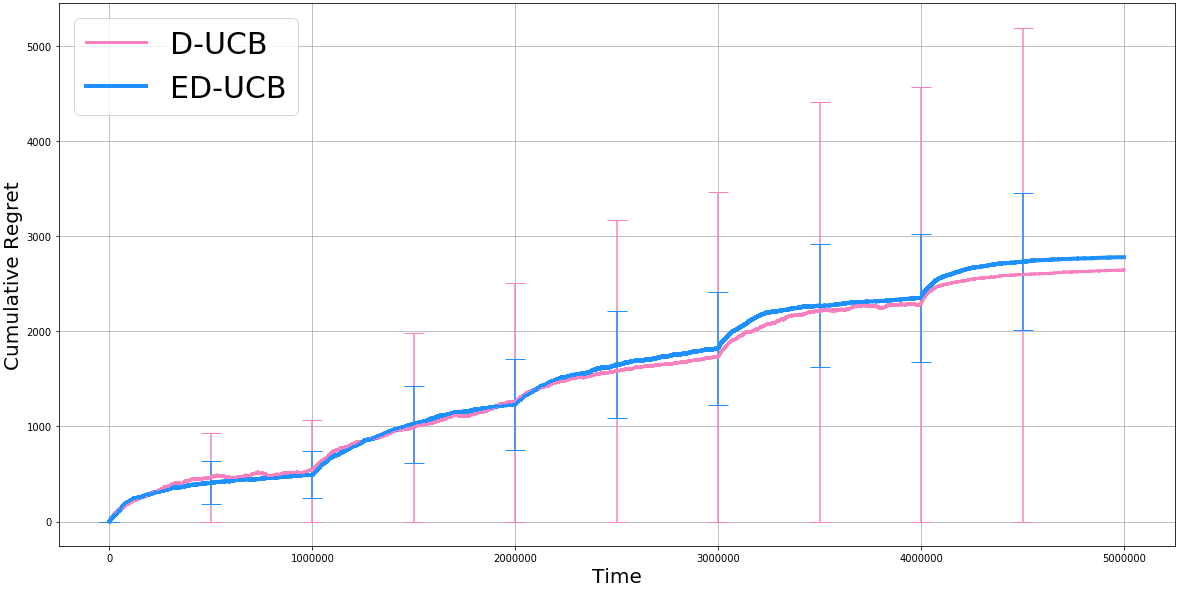
Figure 2: Experiments on the Movielens 1M data set: A zoomed in version of Figure 1 comparing the performance of ED-UCB vs D-UCB. The error bars indicate one standard deviation.

Proof of Theorem 7: Lemma 6 gives us that with probability at least $1-\frac{1}{T\sqrt{E}}$, each expert has at least $n$ samples before the agent interacts with the environment. Under this event, using Lemma 8, the agent can build empirical experts with maximum error $\xi$ w.p. at least $1-T^{-1}$. Therefore, conditioning on the event $\mathcal{E}$ and then on the event that the approximate experts are accurate, we have the following chain:

$$R(E,T) =\sum_{e\in[E]}R_{e}(T)$$

$$\leq\frac{1}{T\sqrt{E}}\times ET+\left(1-\frac{1}{T\sqrt{E}}\right)\left(\frac{1}{T}\times ET+\left(1-\frac{1}{T}\right)\sum_{e=1}^{E}R(\Delta_{e})\right)$$

$$=\sqrt{E}+\left(E-\frac{\sqrt{E}}{T}\right)+\sum_{e=1}^{E}R(\Delta_{e})$$

$$~{}~{}~{}~{}~{}+\left(\frac{1}{T\sqrt{E}}-\frac{1}{\sqrt{E}}-1\right)\frac{\sum_{e=1}^{E}R(\Delta_{e})}{T}$$

$$\leq\sqrt{E}+E+\left(\sum_{e=1}^{T}R(\Delta_{e})\right)\left(1+\frac{1}{T^{2}\sqrt{E}}\right).$$

$\square$

We skip the proof of Theorem 7.1 as it follows trivially from the above arguments.

Appendix E Experiments

A zoomed in version of Figure 1 is presented in Figure 2. We mention the technical specifications of the machines used to conduct these experiments below.

Technical Specifications: Experiments were performed on an internal cluster with nodes equipped with Intel Xeon E5-2600 v2 series 16-core processors, 256GB RAM running RHEL 7.6.

References

• [Agarwal et al., 2014] Agarwal, A., Hsu, D., Kale, S., Langford, J., Li, L., and Schapire, R. (2014). Taming the monster: A fast and simple algorithm for contextual bandits. In International Conference on Machine Learning, pages 1638–1646. PMLR.
• [Auer et al., 2002a] Auer, P., Cesa-Bianchi, N., and Fischer, P. (2002a). Finite-time analysis of the multiarmed bandit problem. Machine learning, 47(2):235–256.
• [Auer et al., 2002b] Auer, P., Cesa-Bianchi, N., Freund, Y., and Schapire, R. E. (2002b). The nonstochastic multiarmed bandit problem. SIAM journal on computing, 32(1):48–77.
• [Azar et al., 2013] Azar, M. G., Lazaric, A., and Brunskill, E. (2013). Sequential transfer in multi-armed bandit with finite set of models. In Proceedings of the 26th International Conference on Neural Information Processing Systems-Volume 2, pages 2220–2228.
• [Baxter, 1998] Baxter, J. (1998). Theoretical models of learning to learn. In Learning to learn, pages 71–94. Springer.
• [Bubeck and Cesa-Bianchi, 2012] Bubeck, S. and Cesa-Bianchi, N. (2012). Regret analysis of stochastic and nonstochastic multi-armed bandit problems. arXiv preprint arXiv:1204.5721.
• [Bubeck et al., 2013] Bubeck, S., Cesa-Bianchi, N., and Lugosi, G. (2013). Bandits with heavy tail. IEEE Transactions on Information Theory, 59(11):7711–7717.
• [Cappé et al., 2013] Cappé, O., Garivier, A., Maillard, O.-A., Munos, R., Stoltz, G., et al. (2013). Kullback–leibler upper confidence bounds for optimal sequential allocation. The Annals of Statistics, 41(3):1516–1541.
• [Cayci et al., 2019] Cayci, S., Eryilmaz, A., and Srikant, R. (2019). Learning to control renewal processes with bandit feedback. Proceedings of the ACM on Measurement and Analysis of Computing Systems, 3(2):1–32.
• [Cella et al., 2020] Cella, L., Lazaric, A., and Pontil, M. (2020). Meta-learning with stochastic linear bandits. In International Conference on Machine Learning, pages 1360–1370. PMLR.
• [Charles et al., 2013] Charles, D., Chickering, M., and Simard, P. (2013). Counterfactual reasoning and learning systems: The example of computational advertising. Journal of Machine Learning Research, 14.
• [Chu et al., 2011] Chu, W., Li, L., Reyzin, L., and Schapire, R. (2011). Contextual bandits with linear payoff functions. In Proceedings of the Fourteenth International Conference on Artificial Intelligence and Statistics, pages 208–214. JMLR Workshop and Conference Proceedings.
• [Deshmukh et al., 2017] Deshmukh, A. A., Dogan, U., and Scott, C. (2017). Multi-task learning for contextual bandits. arXiv preprint arXiv:1705.08618.
• [Dudik et al., 2011] Dudik, M., Hsu, D., Kale, S., Karampatziakis, N., Langford, J., Reyzin, L., and Zhang, T. (2011). Efficient optimal learning for contextual bandits. arXiv preprint arXiv:1106.2369.
• [Foster et al., 2018] Foster, D., Agarwal, A., Dudik, M., Luo, H., and Schapire, R. (2018). Practical contextual bandits with regression oracles. In International Conference on Machine Learning, pages 1539–1548. PMLR.
• [Foster and Rakhlin, 2020] Foster, D. and Rakhlin, A. (2020). Beyond ucb: Optimal and efficient contextual bandits with regression oracles. In International Conference on Machine Learning, pages 3199–3210. PMLR.
• [Harper and Konstan, 2015] Harper, F. M. and Konstan, J. A. (2015). The movielens datasets: History and context. Acm transactions on interactive intelligent systems (tiis), 5(4):1–19.
• [Kveton et al., 2021] Kveton, B., Konobeev, M., Zaheer, M., Hsu, C.-w., Mladenov, M., Boutilier, C., and Szepesvari, C. (2021). Meta-thompson sampling. arXiv preprint arXiv:2102.06129.
• [Langford and Zhang, 2007] Langford, J. and Zhang, T. (2007). Epoch-greedy algorithm for multi-armed bandits with side information. Advances in Neural Information Processing Systems (NIPS 2007), 20:1.
• [Lattimore et al., 2016] Lattimore, F., Lattimore, T., and Reid, M. D. (2016). Causal bandits: Learning good interventions via causal inference. arXiv preprint arXiv:1606.03203.
• [Mahmood et al., 2014] Mahmood, A. R., Van Hasselt, H., and Sutton, R. S. (2014). Weighted importance sampling for off-policy learning with linear function approximation. In NIPS, pages 3014–3022.
• [Mazumder et al., 2010] Mazumder, R., Hastie, T., and Tibshirani, R. (2010). Spectral regularization algorithms for learning large incomplete matrices. Journal of machine learning research, 11(Aug):2287–2322.
• [Perlich et al., 2014] Perlich, C., Dalessandro, B., Raeder, T., Stitelman, O., and Provost, F. (2014). Machine learning for targeted display advertising: Transfer learning in action. Machine learning, 95(1):103–127.
• [Rubinsteyn and Feldman, 2016] Rubinsteyn, A. and Feldman, S. (2016). fancyimpute: An imputation library for python.
• [Sen et al., 2017] Sen, R., Shanmugam, K., Dimakis, A. G., and Shakkottai, S. (2017). Identifying best interventions through online importance sampling. In International Conference on Machine Learning, pages 3057–3066. PMLR.
• [Sen et al., 2018] Sen, R., Shanmugam, K., and Shakkottai, S. (2018). Contextual bandits with stochastic experts. In International Conference on Artificial Intelligence and Statistics, pages 852–861. PMLR.
• [Simchi-Levi and Xu, 2020] Simchi-Levi, D. and Xu, Y. (2020). Bypassing the monster: A faster and simpler optimal algorithm for contextual bandits under realizability. Available at SSRN.
• [Thrun, 1998] Thrun, S. (1998). Lifelong learning algorithms. In Learning to learn, pages 181–209. Springer.
• [Weissman et al., 2003] Weissman, T., Ordentlich, E., Seroussi, G., Verdu, S., and Weinberger, M. J. (2003). Inequalities for the l1 deviation of the empirical distribution. Hewlett-Packard Labs, Tech. Rep.
• [Yang et al., 2020] Yang, J., Hu, W., Lee, J. D., and Du, S. S. (2020). Provable benefits of representation learning in linear bandits. arXiv preprint arXiv:2010.06531.
• [Zhang et al., 2019] Zhang, C., Agarwal, A., Daumé III, H., Langford, J., and Negahban, S. N. (2019). Warm-starting contextual bandits: Robustly combining supervised and bandit feedback. arXiv preprint arXiv:1901.00301.
• [Zhang et al., 2014] Zhang, W., Yuan, S., and Wang, J. (2014). Optimal real-time bidding for display advertising. In Proceedings of the 20th ACM SIGKDD international conference on Knowledge discovery and data mining, pages 1077–1086.