“Are you sure?”: Preliminary Insights from Scaling Product Comparisons to Multiple Shops
Abstract.
Large eCommerce players introduced comparison tables as a new type of recommendations. However, building comparisons at scale without pre-existing training/taxonomy data remains an open challenge, especially within the operational constraints of shops in the long tail. We present preliminary results from building a comparison pipeline designed to scale in a multi-shop scenario: we describe our design choices and run extensive benchmarks on multiple shops to stress-test it. Finally, we run a small user study on property selection and conclude by discussing potential improvements and highlighting the questions that remain to be addressed.
1. Introduction
Online shopping has seen tremendous growth in recent years (Statista Research Department, 2020), and shoppers now face an innumerable number of possibilities, which paradoxically may lead to decreasing satisfaction in their purchase decisions (Scheibehenne et al., 2010). Recommender systems (RSs) have been playing an indispensable role in fighting information overload, and large players (Pichestapong, 2019; Hosanagar et al., 2014) have been mostly responsible for modelling and product innovation (Tsagkias et al., 2020; Bhagat et al., 2018). Comparison engines (CEs) are a special case of RS, in which a product detail page (PDP) displays alternative choices in a table containing informative product specifications (Fig. 1). Unlike prevalent ”More like this” RSs, comparison tables when well-designed not only promote products that are relevant, but also intentionally select products which help customers better understand the range of available features. However – as demonstrated by the sub-optimal alternatives in Fig. 1 – building a CE is far from trivial even for players with full ownership of the data chain. In this paper, we share preliminary lessons learned when building CEs in a B2B scenario, that is, designing a scalable pipeline that is deployed across multiple shops. As convincingly argued in (Tagliabue et al., 2020b; Bianchi et al., 2020; Tagliabue et al., 2021), multi-tenant deployments require models to generalize to dozens of different retailers: a successful CE is therefore not only hard to build, but valuable to a wide range of practitioners – on one side, practitioners outside of humongous websites, who want to enhance their shop in the face of rising pressure from major players; on the other, multi-tenant SaaS providers who need to provide AI-based services that scale to a large number of clients.111As an indication of the relevant SaaS market size, we witnessed Coveo, Algolia, Lucidworks and Bloomreach raising more than 100M USD each from venture funds in the last two years for AI-powered services (Techcrunch, [n.d.], 2019a, 2019b, 2021). We summarize our contributions as follows:
-
•
we are the first, to the best of our knowledge, to detail a pipeline for building a comparison engine designed to be scalable in a multi-tenant scenario;
-
•
we perform extensive experiments on various data cleaning and augmentation approaches. One of our major practical contributions – in line with what independently reported by Hao et al. (2020) – is questioning the widely held belief that co-occurrence patterns are a sufficient proxy for substitutable products (McAuley et al., 2015);
-
•
we discuss the importance of diversity in the comparison table and propose a decision process to determine relevant attributes.

Example of product comparisons on Amazon.com.
While we do acknowledge that full online testing is needed to answer some outstanding design questions, we supplement our pipeline tests with a user study, allowing for a preliminary comparison between our results and human judgments, as well as guiding future decisions in our roadmap. Practitioners looking to replicate our work are encouraged to check the Appendix for details on our tools, modelling choices and Mechanical Turk setup.
2. Comparison Engine Pipeline
In this section, we present the pipeline architecture of our comparison system. The pipeline is composed of three main stages: a first candidate fast retrieval phase, to narrow down the search space; a candidate refinement phase, to ensure precision and produce the final shortlist of products; lastly, a final selection phase, to determine the information to be displayed in the comparison table. We will first explain the logic of each stage, then detail the experiments performed to benchmark the pipeline.222Note that due to space constraints, we cite the most relevant literature inline at the most appropriate step.
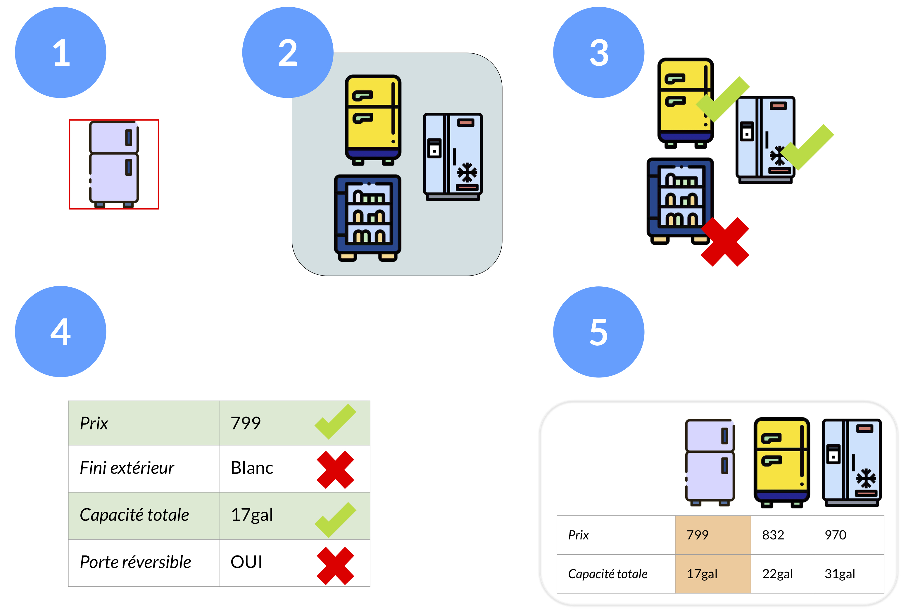
Overview of our CE pipeline.
| Shop A | Shop B | |||||
| Configuration | P@R=0.7 | P@R=0.8 | P@R=0.9 | P@R=0.7 | P@R=0.8 | P@R=0.9 |
| Baseline | 0.744 | 0.743 | 0.682 | 0.611 | 0.573 | 0.539 |
| C=0; S=0 | 0.759 (0.0235) | 0.710(0.0212) | 0.645 (0.0195) | 0.734 (0.0324) | 0.690 (0.0333) | 0.632 (0.0290) |
| C=0; S=1 | 0.766 (0.0257) | 0.723 (0.0237) | 0.659 (0.0189) | 0.755 (0.0379) | 0.706 (0.0423) | 0.643 (0.0382) |
| C=1; S=0 | 0.833 (0.0162) | 0.802 (0.0226) | 0.740 (0.0301) | 0.777 (0.0162) | 0.732 (0.0131) | 0.658 (0.0123) |
| C=1; S=1 | 0.842 (0.0150) | 0.812 (0.0208) | 0.753 (0.0280) | 0.789 (0.0189) | 0.743 (0.0196) | 0.663 (0.0176) |
2.1. Fast Retrieval
Candidate retrieval aims to quickly generate potential substitutes given a query product, with a focus on recall (step in Fig. 2): we try to get a more diverse set, knowing false positives will be screened out in later phases. A common practice for fast retrieval in a dense space is using k-NN over an embedding space (Zhao et al., 2018; Covington et al., 2016): since recent literature (Bianchi et al., 2020; Bianchi et al., 2021; Tagliabue et al., 2020a) provides extensive evidence on the representational qualities of behavioral embeddings, we train a prod2vec space (Grbovic et al., 2015) by adapting word2vec (Mikolov et al., 2013) to eCommerce – i.e. a prod2vec space is just a word2vec space, where words in a sentence are replaced with products in a shopping session (Appendix B). After obtaining a prod2vec space we apply k-NN (based on cosine distance) to retrieve the closest products as its substitute candidates. Analogous to words in word2vec, products which are distributionally similar (based on historical sessions) are close in the prod2vec space, therefore the candidates retrieved in this step are already biased towards substitutable products.
2.2. Candidate Refinement
Candidates produced by the first stage are passed to the second stage for fine-grained processing. The goal of this stage is to boost precision by filtering out candidates that do not have matching product type, and re-rank the remaining ones so the most comparable ones are at the top of the list (step in Fig. 2). We employ a binary classification model (i.e. given a pair of products, are they substitutes?) built on top of a Siamese Network (Bromley et al., 1993), fed with unsupervised behavioral data.
2.2.1. Unsupervised Behavioural Data
Generating training data for substitute product detection is a well-explored topic in the literature (McAuley et al., 2015; Chen et al., 2020; Zhang et al., 2019). However, our inference is somewhat harder than a general substitute classifier where products are sampled from the entire catalog, as our model needs to be able to make subtler distinctions among a selected group of candidates that have been shortlisted by a coarse similarity measure (Section 2.1). To overcome the problem of naive sampling and reduce the noise in behavioral data, we built a three-step process generating the final training set, with free parameters, , , (Appendix B):
-
(1)
We use co-view and co-purchase patterns to obtain positive and negative training examples. Positive examples are obtained from pairs of products which are viewed consecutively (co-view: if I want a TV, I will check several TVs in a row) and negative examples are obtained from products which are purchased consecutively (co-purchase: if I just bought a TV, I am unlikely to buy a second one). To reduce noise, we set a minimum threshold for the number of co-view occurrences () and the number of co-purchase occurrences () for a pair to be considered a positive or negative example respectively.
-
(2)
We intuit that substitutable products are a priori visually similar, and utilize this to further reduce noise in the data. Thus, we apply a threshold on the cosine similarity of the image embedding of pairs to further refine this set of training examples. Given an image vector obtained through a pre-trained VGG16 (Simonyan and Zisserman, 2015), we enforce that positive/negative pairs must have a minimum/maximum cosine similarity.333While drafting this paper, we realized a similar approach has been recommended independently by (Zuo et al., 2020). We refer to this refinement/cleaning process as C.
-
(3)
We remove pairs which are given both positive and negative labels, then build a graph using the remaining positive pairs and extract disconnected subgraphs as clusters of substitutable products. We eliminate clusters of size when generating synthetic pairs, to reduce the risk of sampling from clusters formed by noisy pairs and, at the same time, improve the balance of product types in the training data. By taking an existing positive/negative pair from our behavioural logs, we generate synthetic pairs by swapping out one of the products in the original pair with any product found in its substitute cluster, unlike (Guo et al., 2020) which samples negative examples from a random disconnected subgraph. We refer to this augmentation process as S.
We emphasize that only behavioral logs and product images are necessary so far: our approach does not assume peculiar meta-data or pre-made taxonomy, nor does our classifier require costly labelling, making the pipeline suitable for multi-shop scaling.
2.2.2. Binary Classifier: A Siamese Network
We utilize a binary classifier to predict whether two input products are substitutes or not. Products are represented by various dense representations of product features, such as behavioural embeddings and word2vec embeddings for product title, description and category strings (See Appendix B). For full reproducibility, we provide architectural and hyper-parameter details in Appendices B & C.
2.3. Product and Property Selection
2.3.1. Relevant Property Selection
At this stage, we make the only significant meta-data assumption of the entire pipeline, that is, the target catalog should specify product properties in some structured way – based on our experience with dozens of deployments, this is not a universal feature, but it is common for verticals with technical products (DIY, electronics, etc.), for which CEs are most useful. Given a mapping from products to their properties (say, from TV to the set ¡resolution, screen size, …¿), this stage determines which properties are relevant to shoppers when they are making a purchase decision (step in Fig. 2). By passing the candidates from Section 2.1 to the classifier in 2.2, we generate a final list of substitutable products, given an initial query product. For this list, we rank properties based on the weighted sum of three components444Weights have been determined empirically at first, but see Section 3.2 and our conclusion for potential use of human-in-the-loop inference., highlighted as important by previous literature (Katukuri et al., 2014; Dong et al., 2020) and domain knowledge:
-
(1)
Query frequency: properties which are important to shoppers tend to appear frequently in shopper-generated content (Bing et al., 2016; Moraes et al., 2020) such as queries (Katukuri et al., 2014). We calculate the query frequency for each property (and their possible values) by mining search logs, and normalize the counts to range ;
-
(2)
PDP frequency: merchandisers are more likely to explicitly mention important attributes in the PDP. We calculate a normalized count for each attribute by mining product descriptions in the catalog;
-
(3)
Property entropy: it is important, for meaningful comparison, that property values have enough variation, so that comparison tables can help navigate easily the possible dimensions of a catalog. To calculate variety, we measure the entropy of the distribution of property values across the list of substitute products.
2.3.2. Final Display Selection
Recent literature (Wu et al., 2019) has highlighted the importance of diversity in RSs. Thus, after determining important product properties, we select the final substitutes per query item (step in Fig. 2), by making two additional calculations: price diversification and representative selection. Given the list of substitutes, we group products into 7 bins based on their log price.555The mean log-price is used to set the central bin and the standard deviation is used to determine the bin width. We discard the first and the last bin, as extreme prices can signal a potential mismatch in product category. With 5 bins remaining, we sample one substitute from the same price bin as the query item, and two substitutes from its higher-pricing and lower-pricing neighbor bin. Finally, similarly to (Chen and Karger, 2006), we employ a greedy approach during sampling, which maximises the information diversity among the final products to be displayed. We represent the property values of each product via one-hot encoding, so that products are represented by a concatenation of their one-hot encoded property vectors. We compute the difference in their information content by Hamming distance, where each property is weighted by the negative exponential of the entropy of the distribution of the property’s values. The intuition is that we want to vary properties which are far from quasi-uniform distributions to display products with meaningful variation, thereby giving shoppers a more complete picture of what is available.
3. Experiments
After having discussed the pipeline design, we report our experiments for the substitute model and the user study performed on property selection.
3.1. Substitute model
We evaluate the effectiveness of training a neural model for substitute classification in an unsupervised manner, by leveraging a manually prepared held out set for benchmarks (Section 3.1.1)666Since in a real deployment labels will not be present, a research setting is needed to first validate how well unsupervised training performs on golden data.. Since the objective of the substitute model is to refine the candidates from the initial fast retrieval step (Section 2.1), where candidates are a priori likely, but not guaranteed, to be substitutes, our test set also mimics this distribution. As a baseline, we thus adopt the cosine similarity (re-scaled to ) between the image vectors of two products as the confidence score for substitutability. This serves as a simple yet realistic baseline that allows us to quantitatively assess the precision boost afforded by the substitute model.
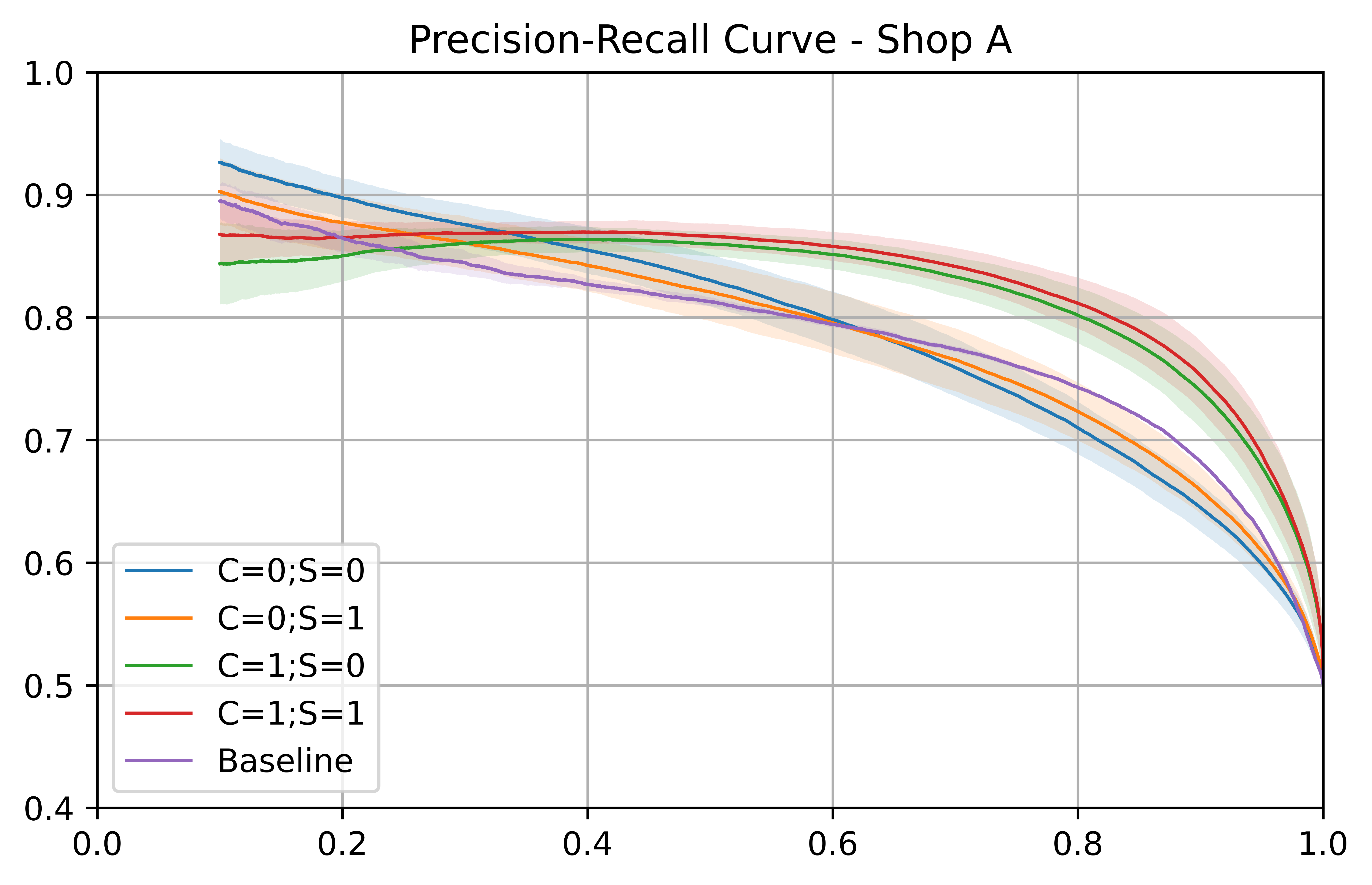
For our experiments, we consider all configurations of image vectors for cleaning () and synthetic augmentation () to shed light on their contribution to performance.7771 denotes usage/application of method whereas 0 denotes non-usage. We run experiments on 3 different seeds and with various combinations of dense product representation (Appendix B & C) as input. For each configuration of C and S, we report average performance across seeds and product representations used, as well the confidence intervals in plots. We run an extensive set of experiments to acknowledge the varying quality of such representations across catalogs, and to demonstrate robustness of certain configurations when scaling CEs in a multi-shop scenario.
3.1.1. Dataset
For training and validation, we extract unsupervised co-view and co-purchase data from shopping sessions of two partnering shops, Shop A and Shop B. They are mid-sized shops: Shop A is in the sport apparel industry whereas Shop B is in home improvement. We use of all products for training and the remaining for validation. We consider this to be a strict testing regime as none of the products used in validation and testing are seen in training. For testing, we first obtain a golden mapping of clusters of substitutable products by heuristic matching of categories provided in catalog data and extensive manual filtering. The golden mapping is then used to generate positive and negative test examples as explained in Section 2.1.888Full descriptive statistics are reported in Appendix B. We selected shops with catalogs that are of high quality and contain fine-grained category information in order to generate golden mappings which best capture product substitutability. We emphasize that such catalog quality is not guaranteed across shops, which motivates our use of unsupervised data.
3.1.2. Results
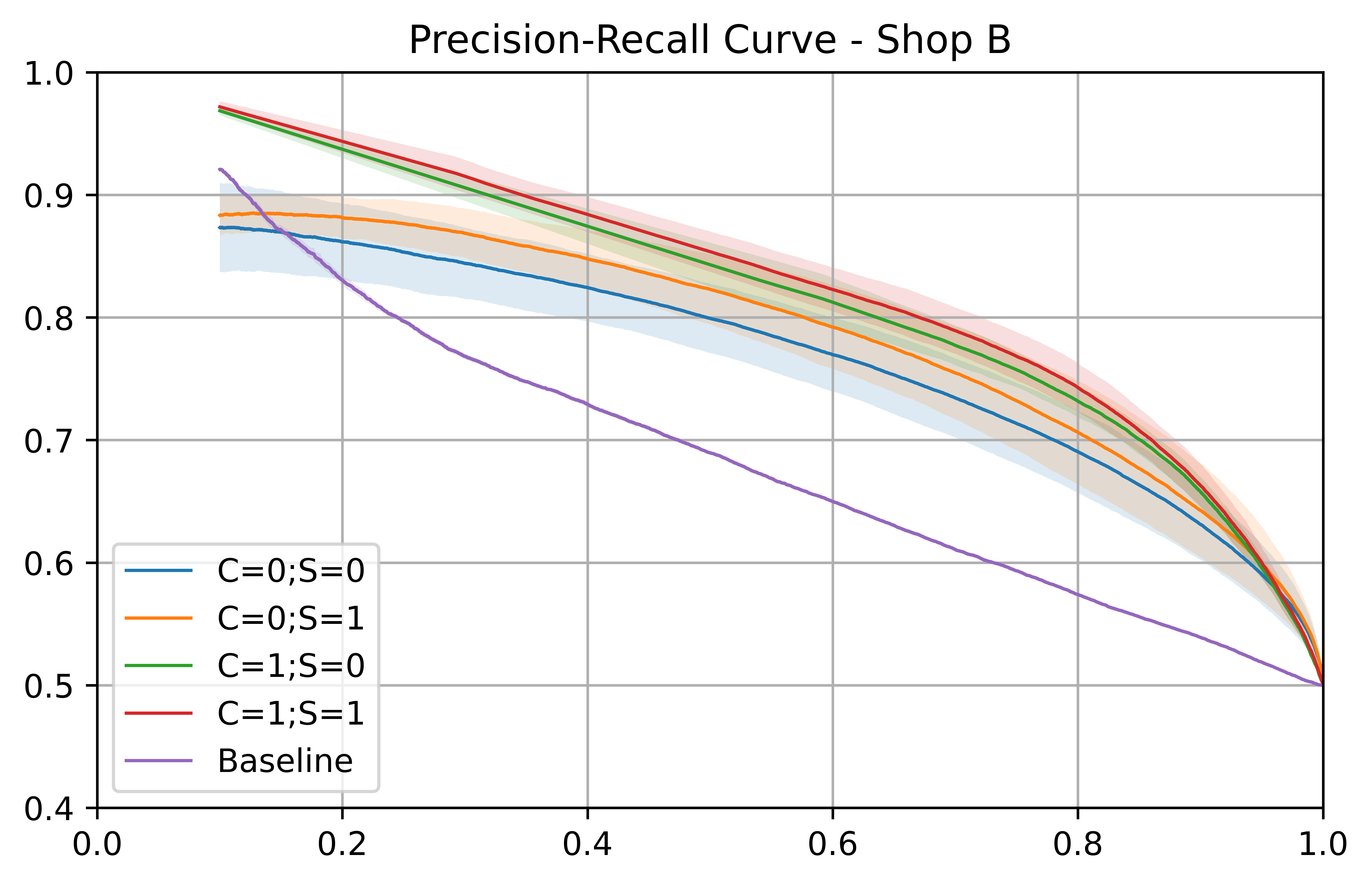
We summarize experimental results in Table 1, and plot in Fig. 3 the Precision-Recall (PR) curves. For Shop A, when image vectors are not used for cleaning (), the model performs only as good as the baseline. When , we see a significant increase in precision across the higher ranges of recall; on the other hand, synthetic augmentation, , has minimal effect on model performance. Similar trends are observed for Shop B, albeit the benefit of is less pronounced. These results demonstrate the effectiveness of using image vectors to clean the otherwise noisy unsupervised co-occurrence data, and validate the effectiveness of the preparation detailed in Section 2.2. However, as evident in the baseline performance of Shop B, caution must still be taken when relying on image vectors – depending on the vertical, visual similarity may not be as strong a proxy for substitutability and/or the pre-trained models used to generate the image embeddings are not fine-tuned for products in certain verticals. This opens up interesting avenues for future work such as self-supervised learning (Zbontar et al., 2021) for niche verticals.
3.2. Property selection
We run an Amazon Mechanical Turk (MTurk) study to get preliminary insights on how well our algorithm matches how shoppers rank properties. Our investigation involves 4 product types that range from known products (e.g. running shoes) to increasingly technical (e.g. ski), each with 5-8 properties. While agreement with human judgement varies depending on the category, the algorithm seems to pick up at least some qualitatively relevant latent dimension.
3.2.1. Data Collection
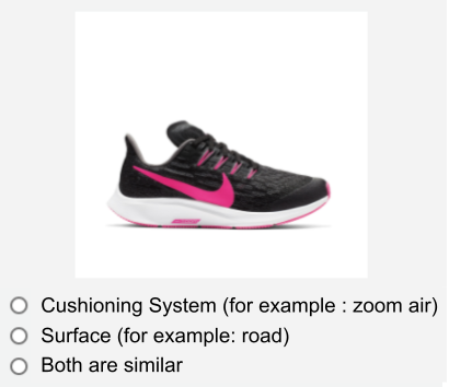
We collect pairwise human judgements on property preferences. For each comparison, we present workers with the image of a product and two of its properties and ask them to judge which is more important to them when making a purchase decision. Each Human Intelligence Task (HIT) has 3 comparisons (Fig. 4) in addition to a control task to filter out low quality responses. We collected an average of 30 responses per property pair for this experiment. To collate pairwise human responses, we estimate the underlying ranking using the Bradley-Terry Model (Bradley and Terry, 1952; Maystre, 2015). We compare the estimated ranked list against our algorithm using Rank-biased Overlap (Webber et al., 2010) (RBO) as the measure of agreement.
3.2.2. Results
The results are summarized in Table 2. Agreement between our algorithm and humans is higher for popular/common products, lower for highly-technical ones, which may also reflect a lack of domain-specific knowledge by general MTurk workers.999Anecdotally, we also solicited feedback from active skiers in Coveo, and found that their experience influenced the properties which they found important. Interestingly enough, the RBO for Running Shoes is by far the highest. We suspect that this is because Running Shoes lie at an intersection of being both well-known, whereby crowded-sourced responses are most reliable, and technical, such that there exists a stronger ranking/ordering of its properties.
| Product | RBO |
|---|---|
| Shirt | 0.633 |
| Shorts | 0.483 |
| Running Shoe | 0.783 |
| Ski | 0.169 |
4. Conclusion
We shared insights from building a CE addressing large-to-mid-shops in the market long-tail, and as such particularly suited for multi-shop deployment. While preliminary, our multi-shop benchmarks confirms the viability of our pipeline, and we look forward to testing it online. Two important areas of improvements are personalization and human-in-the-loop inference. In the current system, all shoppers would receive the same set of candidates, but individual preferences and session intent (Tagliabue et al., 2020a) may be used to further shape the final table.
Finally, of the three ways in which we could use human judgements – qualitative validation, training data and active learning – we just focused on the first. Given the scalability of MTurk, however, we plan on extending human-in-the-loop computation in further iterations of the project.
5. Ethical Considerations
User data has been collected in the process of providing business services to the clients of Coveo: user data is collected and processed in an anonymized fashion, in full compliance with existing legislation (GDPR). In particular, the target dataset uses only anonymous uuids to label sessions and, as such, it does not contain any information that can be linked to individuals. As explained, our MTurk HITs include a task with pre-defined answer to control for workers randomly answering to questions; however, we still compensate workers for their time, even if their answers get discarded from the analysis.
Acknowledgements.
We wish to thank Federico Bianchi, Mattia Pavoni and Andrea Polonioli for comments on a previous draft of this work, and general support with this research project.References
- (1)
- Berg et al. (2019) David Berg, Ravi Kiran Chirravuri, Romain Cledat, Savin Goyal, Ferras Hamad, and Ville Tuulos. 2019. Open-Sourcing Metaflow, a Human-Centric Framework for Data Science. https://netflixtechblog.com/open-sourcing-metaflow-a-human-centric-framework-for-data-science-fa72e04a5d9
- Bhagat et al. (2018) Rahul Bhagat, Srevatsan Muralidharan, Alex Lobzhanidze, and Shankar Vishwanath. 2018. Buy It Again: Modeling Repeat Purchase Recommendations. In Proceedings of the 24th ACM SIGKDD International Conference on Knowledge Discovery & Data Mining (London, United Kingdom) (KDD ’18). Association for Computing Machinery, New York, NY, USA, 62–70. https://doi.org/10.1145/3219819.3219891
- Bianchi et al. (2021) Federico Bianchi, Jacopo Tagliabue, and Bingqing Yu. 2021. Query2Prod2Vec: Grounded Word Embeddings for eCommerce. In NAACL-HLT. Association for Computational Linguistics.
- Bianchi et al. (2020) Federico Bianchi, J. Tagliabue, Bingqing Yu, Luca Bigon, and Ciro Greco. 2020. Fantastic Embeddings and How to Align Them: Zero-Shot Inference in a Multi-Shop Scenario. ArXiv abs/2007.14906 (2020).
- Bing et al. (2016) Lidong Bing, Tak-Lam Wong, and Wai Lam. 2016. Unsupervised Extraction of Popular Product Attributes from E-Commerce Web Sites by Considering Customer Reviews. ACM Trans. Internet Technol. 16, 2, Article 12 (April 2016), 17 pages. https://doi.org/10.1145/2857054
- Bradley and Terry (1952) Ralph Allan Bradley and Milton E. Terry. 1952. Rank Analysis of Incomplete Block Designs: I. The Method of Paired Comparisons. Biometrika 39, 3/4 (1952), 324–345. http://www.jstor.org/stable/2334029
- Bromley et al. (1993) Jane Bromley, James W. Bentz, Léon Bottou, Isabelle Guyon, Yann LeCun, Cliff Moore, Eduard Säckinger, and Roopak Shah. 1993. Signature Verification Using A ”Siamese” Time Delay Neural Network. IJPRAI 7, 4 (1993), 669–688. http://dblp.uni-trier.de/db/journals/ijprai/ijprai7.html#BromleyBBGLMSS93
- Chen and Karger (2006) Harr Chen and David R. Karger. 2006. Less is More: Probabilistic Models for Retrieving Fewer Relevant Documents. In Proceedings of the 29th Annual International ACM SIGIR Conference on Research and Development in Information Retrieval (Seattle, Washington, USA) (SIGIR ’06). Association for Computing Machinery, New York, NY, USA, 429–436. https://doi.org/10.1145/1148170.1148245
- Chen et al. (2020) Tong Chen, H. Yin, Guanhua Ye, Zi Huang, Yang Wang, and Ming-Chieh Wang. 2020. Try This Instead: Personalized and Interpretable Substitute Recommendation. Proceedings of the 43rd International ACM SIGIR Conference on Research and Development in Information Retrieval (2020).
- Covington et al. (2016) Paul Covington, Jay Adams, and Emre Sargin. 2016. Deep Neural Networks for YouTube Recommendations. In Proceedings of the 10th ACM Conference on Recommender Systems. New York, NY, USA.
- Dageville et al. (2016) Benoit Dageville, Thierry Cruanes, Marcin Zukowski, Vadim Antonov, Artin Avanes, Jon Bock, Jonathan Claybaugh, Daniel Engovatov, Martin Hentschel, Jiansheng Huang, Allison W. Lee, Ashish Motivala, Abdul Q. Munir, Steven Pelley, Peter Povinec, Greg Rahn, Spyridon Triantafyllis, and Philipp Unterbrunner. 2016. The Snowflake Elastic Data Warehouse. In Proceedings of the 2016 International Conference on Management of Data (San Francisco, California, USA) (SIGMOD ’16). Association for Computing Machinery, New York, NY, USA, 215–226. https://doi.org/10.1145/2882903.2903741
- Dong et al. (2020) X. Dong, Xiang He, A. Kan, Xian Li, Yan Liang, Jun Ma, Y. Xu, Chenwei Zhang, Tong Zhao, Gabriel Blanco Saldana, S. Deshpande, A. M. Manduca, Jay Ren, S. P. Singh, F. Xiao, Haw-Shiuan Chang, Giannis Karamanolakis, Yuning Mao, Yaqing Wang, Christos Faloutsos, A. McCallum, and J. Han. 2020. AutoKnow: Self-Driving Knowledge Collection for Products of Thousands of Types. Proceedings of the 26th ACM SIGKDD International Conference on Knowledge Discovery & Data Mining (2020).
- Grbovic et al. (2015) Mihajlo Grbovic, Vladan Radosavljevic, Nemanja Djuric, Narayan Bhamidipati, Jaikit Savla, Varun Bhagwan, and Doug Sharp. 2015. E-commerce in Your Inbox: Product Recommendations at Scale. In Proceedings of KDD ’15. https://doi.org/10.1145/2783258.2788627
- Guo et al. (2020) Mingming Guo, Nian Yan, Xiquan Cui, San He Wu, Unaiza Ahsan, Rebecca West, and Khalifeh Al Jadda. 2020. Deep Learning-based Online Alternative Product Recommendations at Scale. In Proceedings of The 3rd Workshop on e-Commerce and NLP. Association for Computational Linguistics, Seattle, WA, USA, 19–23. https://doi.org/10.18653/v1/2020.ecnlp-1.3
- Hao et al. (2020) Junheng Hao, Tong Zhao, Jin Li, Xin Luna Dong, Christos Faloutsos, Yizhou Sun, and Wei Wang. 2020. P-Companion: A Principled Framework for Diversified Complementary Product Recommendation. Association for Computing Machinery, New York, NY, USA, 2517–2524. https://doi.org/10.1145/3340531.3412732
- Hosanagar et al. (2014) Kartik Hosanagar, Daniel Fleder, Dokyun Lee, and Andreas Buja. 2014. Will the Global Village Fracture Into Tribes? Recommender Systems and Their Effects on Consumer Fragmentation. Management Science 60 (04 2014), 805–823. https://doi.org/10.1287/mnsc.2013.1808
- Katukuri et al. (2014) Jayasimha Katukuri, Tolga Könik, Rajyashree Mukherjee, and Santanu Kolay. 2014. Recommending Similar Items in Large-scale On line Marketplaces. https://doi.org/10.13140/2.1.3259.2646
- Maystre (2015) Lucas Maystre. 2015. choix. (2015). https://github.com/lucasmaystre/choix
- McAuley et al. (2015) Julian McAuley, Rahul Pandey, and Jure Leskovec. 2015. Inferring Networks of Substitutable and Complementary Products. In Proceedings of the 21th ACM SIGKDD International Conference on Knowledge Discovery and Data Mining (Sydney, NSW, Australia) (KDD ’15). Association for Computing Machinery, New York, NY, USA, 785–794. https://doi.org/10.1145/2783258.2783381
- Mikolov et al. (2013) Tomas Mikolov, Kai Chen, Gregory S. Corrado, and Jeffrey Dean. 2013. Efficient Estimation of Word Representations in Vector Space. CoRR abs/1301.3781 (2013).
- Moraes et al. (2020) Felipe Moraes, Jie Yang, Rongting Zhang, and Vanessa Murdock. 2020. The Role of Attributes in Product Quality Comparisons. In Proceedings of the 2020 Conference on Human Information Interaction and Retrieval (Vancouver BC, Canada) (CHIIR ’20). Association for Computing Machinery, New York, NY, USA, 253–262. https://doi.org/10.1145/3343413.3377956
- Pichestapong (2019) Ann Pichestapong. 2019. Website Personalization: Improving Conversion with Personalized Shopping Experiences. Retrieved November 29, 2020 from https://www.shopify.ca/partners/blog/website-personalization
- Reimers and Gurevych (2019) Nils Reimers and Iryna Gurevych. 2019. Sentence-BERT: Sentence Embeddings using Siamese BERT-Networks. arXiv:1908.10084 [cs.CL]
- Scheibehenne et al. (2010) Benjamin Scheibehenne, Rainer Greifeneder, and Peter M. Todd. 2010. Can There Ever Be Too Many Options? A Meta-Analytic Review of Choice Overload. Journal of Consumer Research 37, 3 (02 2010), 409–425. https://doi.org/10.1086/651235 arXiv:https://academic.oup.com/jcr/article-pdf/37/3/409/5173186/37-3-409.pdf
- Simonyan and Zisserman (2015) Karen Simonyan and Andrew Zisserman. 2015. Very Deep Convolutional Networks for Large-Scale Image Recognition. In International Conference on Learning Representations.
- Statista Research Department (2020) Statista Research Department. 2020. Global retail e-commerce sales 2014-2023. Retrieved November 29, 2020 from https://www.statista.com/statistics/379046/worldwide-retail-e-commerce-sales/
- Tagliabue et al. (2021) Jacopo Tagliabue, Ciro Greco, Jean-Francis Roy, Federico Bianchi, Giovanni Cassani, Bingqing Yu, and Patrick John Chia. 2021. SIGIR 2021 E-Commerce Workshop Data Challenge. In SIGIR eCom 2021.
- Tagliabue et al. (2020a) Jacopo Tagliabue, Bingqing Yu, and Marie Beaulieu. 2020a. How to Grow a (Product) Tree. Personalized Category Suggestions for eCommerce Type-Ahead. In Companion Proceedings of ACL (Seattle, USA). Association for Computing Machinery, New York, NY, USA.
- Tagliabue et al. (2020b) Jacopo Tagliabue, Bingqing Yu, and Federico Bianchi. 2020b. The Embeddings That Came in From the Cold: Improving Vectors for New and Rare Products with Content-Based Inference. In Fourteenth ACM Conference on Recommender Systems (Virtual Event, Brazil) (RecSys ’20). Association for Computing Machinery, New York, NY, USA, 577–578. https://doi.org/10.1145/3383313.3411477
- Techcrunch ([n.d.]) Techcrunch. [n.d.]. coveo-raises-227m-at-1b-valuation. https://techcrunch.com/2019/11/06/coveo-raises-227m-at-1b-valuation-for-ai-based-enterprise-search-and-personalization/
- Techcrunch (2019a) Techcrunch. 2019a. Algolia finds $110M from Accel and Salesforce. https://techcrunch.com/2019/10/15/algolia-finds-110m-from-accel-and-salesforce-for-its-search-as-a-service-used-by-slack-twitch-and-8k-others/
- Techcrunch (2019b) Techcrunch. 2019b. Lucidworks raises $100M to expand in AI finds. https://techcrunch.com/2019/08/12/lucidworks-raises-100m-to-expand-in-ai-powered-search-as-a-service-for-organizations/
- Techcrunch (2021) Techcrunch. 2021. Bloomreach raises $150M on $900M valuation and acquires Exponea. https://techcrunch.com/2021/01/26/bloomreach-raises-150m-on-900m-valuation-and-acquires-exponea/
- Tsagkias et al. (2020) Manos Tsagkias, Tracy Holloway King, Surya Kallumadi, Vanessa Murdock, and Maarten de Rijke. 2020. Challenges and Research Opportunities in eCommerce Search and Recommendations. In SIGIR Forum, Vol. 54.
- Webber et al. (2010) William Webber, Alistair Moffat, and Justin Zobel. 2010. A Similarity Measure for Indefinite Rankings. ACM Trans. Inf. Syst. 28, 4, Article 20 (Nov. 2010), 38 pages. https://doi.org/10.1145/1852102.1852106
- Wu et al. (2019) Qiong Wu, Yong Liu, Chunyan Miao, Yin Zhao, Lu Guan, and Haihong Tang. 2019. Recent Advances in Diversified Recommendation. arXiv:1905.06589 [cs.IR]
- Zbontar et al. (2021) Jure Zbontar, Li Jing, Ishan Misra, Yann LeCun, and Stéphane Deny. 2021. Barlow Twins: Self-Supervised Learning via Redundancy Reduction. CoRR abs/2103.03230 (2021). arXiv:2103.03230 https://arxiv.org/abs/2103.03230
- Zhang et al. (2019) Shijie Zhang, Hongzhi Yin, Qinyong Wang, Tong Chen, Hongxu Chen, and Quoc Viet Hung Nguyen. 2019. Inferring Substitutable Products with Deep Network Embedding. In Proceedings of the Twenty-Eighth International Joint Conference on Artificial Intelligence, IJCAI-19. International Joint Conferences on Artificial Intelligence Organization, 4306–4312. https://doi.org/10.24963/ijcai.2019/598
- Zhao et al. (2018) Xiaoting Zhao, Raphael Louca, D. Hu, and L. Hong. 2018. Learning Item-Interaction Embeddings for User Recommendations. ArXiv abs/1812.04407 (2018).
- Zuo et al. (2020) Zhen Zuo, Lixi Wang, Michinari Momma, Wenbo Wang, Yikai Ni, Jianfeng Lin, and Yi Sun. 2020. A flexible large-scale similar product identification system in e-commerce. KDD 1st International Workshop on Industrial Recommendation (2020).
Appendix A Implementation Details
We implement our pipeline leveraging Metaflow (Berg et al., 2019), which allows us to programmatically define our pipeline as a DAG. We develop our pipeline with three core phases (spread across several steps):
-
•
we dedicate initial steps in the DAG to pull data (such as user sessions, pre-cached embeddings) from various sources like Snowflake and S3, and perform various transformations on the data. Note that many of these steps run in parallel;
-
•
we launch in parallel our model training (which may in itself contain several steps as outlined in Section 2) with various configurations (e.g. input features). In addition, we are able to dedicate steps which have high resource demands (e.g. GPU) to AWS Batch;
-
•
we collate the results (e.g. metrics, trained model, model predictions) from each parallel run, and store them as Data Artifacts on S3 for further analysis.
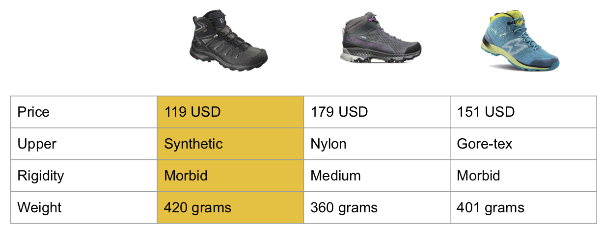
The adoption of Metaflow on top of our cloud provider (AWS) speeds up development time (since it is the same code running locally and remotely), reduces training time (thanks to parallelism and GPU provisioning) and increases confidence in our experiments (thanks to versioning and full pipeline replayability). The setup we adopt fully decouples writing code from the underlying infrastructure, including data retrieval thanks to the “PaaS-like feeling” of Snowflake (Dageville et al., 2016). Fig. 5 shows the comparison table for a pair of mountain shoes (yellow), as produced by our Metaflow pipeline.
Appendix B Unsupervised Data and Product Representations
In this section, we provide details and hyper-parameters used in the generation of training data and of dense unsupervised representations for products.
B.1. Data Preparation
-
•
Co-view and Co-purchase Data: For Shop A, we obtain shopping sessions over a period of 3 months and for Shop B we obtain shopping sessions over a period of 1 month. For co-view pairs, we enforce a minimum count, , and for co-purchase pairs we enforce a minimum count .
-
•
Cleaning with Image Vectors: For both Shop A and Shop B, we enforce that positive pairs have a cosine similarity and that negative pairs have a cosine similarity .
-
•
Synthetic Augmentation: Maximum cluster size, , is set to 40.
| Shop | #Products | # Browse Session | # Purchase Session |
|---|---|---|---|
| Shop A | 20k | 1.5M | 27k |
| Shop B | 50k | 3M | 12K |
| Shop | Config | Train (Pos/Neg) | Validation (Pos/Neg) |
|---|---|---|---|
| Shop A | C=0; S=0 | 19k/18k | 1.5k/1k |
| C=0; S=1 | 27k/75k | 2.8k/3.7k | |
| C=1; S=0 | 8k/6k | 0.5k/0.5k | |
| C=1; S=1 | 17k/33k | 1.5k/1.5k | |
| Shop B | C=0; S=0 | 50k/20k | 3k/1k |
| C=0; S=1 | 60k/40k | 6k/5k | |
| C=1; S=0 | 40k/10k | 2.5k/1k | |
| C=1; S=1 | 70k/120k | 7k/7k |
B.2. Unsupervised Product Representations
-
•
Prod2Vec Embeddings: We train behavioural product embeddings using CBOW with negative sampling (Mikolov et al., 2013), swapping the concept of words in a sentence with products in a browsing session. Following best practices of (Bianchi et al., 2020) we adopt the hyper-parameters: window = 5 , iterations = 30, ns_exponent = 0.75, dimensions = 48, with the exception of a smaller window size, so that more emphasis is placed on co-viewed, and hence more likely substitutable products.
-
•
Textual Embeddings: We train Textual Embeddings using CBOW with negative sampling and using product descriptions as our text corpus. We adopt the hyper-parameters: window = 10, iterations = 30, ns_exponent = 0.75, dimensions = 48. We then take the name, description and categories of each product and obtain a dense representation for each meta-data by applying average-pooling over their word representations.
-
•
Image Embeddings: We prepare Image Embeddings by utilising a pre-trained VGG16 (Simonyan and Zisserman, 2015) network, and apply 7x7 2D-MaxPooling to the final MaxPool layer of VGG16 to obtain a 512-dim representation.
Appendix C Model Architecture and Training
C.1. Model Architecture
In this section we provide architectural details on the binary comparison model. At a high level, the model takes in two products as inputs and provides a confidence score indicating of whether the two products are substitutes.
First, each product is represented by embeddings , each of dimension representing a different type of information or modality. Details on how these embeddings are obtained can be found in Appendix B.
Secondly, the embeddings of a product are fused into a single dense representation by a neural network , which is re-used across all products. We define as:
where is a dense re-projection layer (48-dim, ReLU activation), is the concatenation operation, is a dense fusion layer (128-dim, ReLU activation) and refers to L2-Normalization operator.
Lastly, the fused representations of two products, are passed into a neural network , which produces the confidence score. We define as:
That is, we take the element-wise absolute difference (Reimers and Gurevych, 2019) between the two inputs and pass it into a dense classification layer (1-dim) followed by the sigmoid function to produce the binary classification score.
C.2. Model Training
For all experiments, we use Adam optimizer with learning rate of , early stopping with patience of 20 epochs and a batch size of 32. For all experiments we tested the follow configurations of product representations:
-
•
description, name, prod2vec;
-
•
categories, description, name;
-
•
categories, description, name, prod2vec.
The feature set that yielded best results is [categories, description, name, prod2vec].