Ergodic Numerical Approximation to Periodic Measures of Stochastic Differential Equations

Chunrong Feng Department of Mathematical Sciences, Durham University, DH1 3LE, UK Yu Liu Department of Mathematical Sciences, Durham University, DH1 3LE, UK Huaizhong Zhao Department of Mathematical Sciences, Durham University, DH1 3LE, UK Research Centre for Mathematics and Interdisciplinary Sciences, Shandong University, Qingdao, Shandong, 266237, China
Abstract

In this paper, we consider numerical approximation to periodic measure of a time periodic stochastic differential equations (SDEs) under weakly dissipative condition. For this we first study the existence of the periodic measure $\rho_{t}$ and the large time behaviour of ๐’ฐโ€‹(t+s,s,x):=๐”ผโ€‹ฯ•โ€‹(Xts,x)โˆ’โˆซฯ•โ€‹๐‘‘ฯt,assign๐’ฐ๐‘ก๐‘ ๐‘ ๐‘ฅ๐”ผitalic-ฯ•superscriptsubscript๐‘‹๐‘ก๐‘ ๐‘ฅitalic-ฯ•differential-dsubscript๐œŒ๐‘ก\mathcal{U}(t+s,s,x):={\mathbb{E}}\phi(X_{t}^{s,x})-\int\phi d\rho_{t}, where Xts,xsuperscriptsubscript๐‘‹๐‘ก๐‘ ๐‘ฅX_{t}^{s,x} is the solution of the SDEs and $\phi$ is a test function being smooth and of polynomial growth at infinity. We prove $\mathcal{U}$ and all its spatial derivatives decay to 0 with exponential rate on time $t$ in the sense of average on initial time s๐‘ s. We also prove the existence and the geometric ergodicity of the periodic measure of the discretized semi-flow from the Euler-Maruyama scheme and moment estimate of any order when the time step is sufficiently small (uniform for all orders). We thereafter obtain that the weak error for the numerical scheme of infinite horizon is of the order $1$ in terms of the time step. We prove that the choice of step size can be uniform for all test functions $\phi$. Subsequently we are able to estimate the average periodic measure with ergodic numerical schemes.

Keywords: Periodic measure; Fokker-Planck equation; discretized semi-flows; geometrical ergodicity; weak approximation.

Mathematics Subject Classifications (2010): 37H99, 60H10, 60H35.

1 Introduction

Random periodicity is ubiquitous in the real world from daily temperature process to economic cycles. The concepts of random periodic paths and periodic measures were introduced and their ergodicity was obtained recently ([11],[12],[13],[16],[36]). They are two different indispensable ways in the pathwise sense and in distributions to describe random periodicity. The โ€œequivalenceโ€ of the random periodic solutions and periodic measures and their characterisation in terms of purely imaginary eigenvalues of the infinitesimal generator of the Markovian semi-group were obtained in [13]. The presence of pure imaginary eigenvalues distinguishes the random periodic processes/periodic measures regime from that of the stationary processes/mixing invariant measures, in the latter case the Koopman-von Neumann Theorem says the infinitesimal generator has a unique eigenvalue 00 on the imaginary axis.

As in the case of deterministic dynamical systems where periodic motion has been in the central stage of its study, the relevance of random periodic paths and periodic measures to theoretical and applied problems arising in stochastic dynamical systems has begun to be realised. In particular, there has been progress in the study of some topics in stochastic dynamics e.g. bifurcations (Wang [33]), random attractors (Bates, Lu and Wang [3]), stochastic resonance (Cherubini, Lamb, Rasmussen and Sato [7], Feng, Zhao and Zhong [14],[15]), random horseshoes (Huang, Lian and Lu [20]), modelling the El Nรฎno phenomenon (Chekroun, Simonnet and Ghil [6]), isochronicity of stochastic oscillations (Engel and Kuehn [8]), and invariant measures of quasi-periodic stochastic systems (Feng, Qu and Zhao [10]).

However, it is difficult to construct random periodic solutions explicitly for many problems. So numerical approximation is critical in the study of stochastic dynamics in addition to the study of random periodic dynamics theory. There are numerous works on numerical analysis of SDEs on a finite horizon ([22],[26],[21],[27]). A numerical analysis of approximation to invariant measures of SDEs through discretizing the pull-back, was given in [24],[29],[31],[32],[34],[35]. Numerical approximations to stable zero solutions of SDEs were given in [18],[22]. Despite the importance both on the theoretical and applied aspects of the random periodic regime, its numerical analysis has barely been developed. The only result we know is the pathwise approximations of the random periodic solutions of SDEs discussed in [9]. In this paper we study the weak approximation to periodic measures.

We consider the following non-autonomous stochastic differential equations on ${\mathbb{R}}^{d}$

dโ€‹Xt=bโ€‹(t,Xt)โ€‹dโ€‹t+ฯƒโ€‹(Xt)โ€‹dโ€‹Wt,tโ‰ฅs,formulae-sequence๐‘‘subscript๐‘‹๐‘ก๐‘๐‘กsubscript๐‘‹๐‘ก๐‘‘๐‘ก๐œŽsubscript๐‘‹๐‘ก๐‘‘subscript๐‘Š๐‘ก๐‘ก๐‘ \displaystyle dX_{t}=b(t,X_{t})dt+\sigma(X_{t})dW_{t},\quad t\geq s, (1.1)

with initial condition Xs=xsubscript๐‘‹๐‘ ๐‘ฅX_{s}=x where $b:{\mathbb{R}}\times{\mathbb{R}}^{d}\rightarrow{\mathbb{R}}^{d},\sigma:{\mathbb{R}}^{d}\rightarrow{\mathbb{R}}^{d\times d}$, $W_{t}$ is a two-sided Wiener process in ${\mathbb{R}}^{d}$ on the Wiener probability space $(\Omega,\mathcal{F},\mathbb{P})$. We assume that $b$ is $\tau$-periodic in the time variable and weakly dissipative in the space variable. For a technical reason, here we only consider the case when $\sigma$ is time independent as we use the results in [14],[19]. Denote by Xts,xsuperscriptsubscript๐‘‹๐‘ก๐‘ ๐‘ฅX_{t}^{s,x} the solution of (1.1) throughout the paper.

The existence of the periodic measure was studied in [14]. Under the assumption that the drift term is weakly dissipative and the diffusion term is non-degenerate, it was proved that the periodic measure ฯssubscript๐œŒ๐‘ \rho_{s} exists and has a density function, denoted by qโ€‹(s,x)๐‘ž๐‘ ๐‘ฅq(s,x). To obtain qโ€‹(s,x)๐‘ž๐‘ ๐‘ฅq(s,x), one could solve the corresponding infinite horizon Fokker-Planck equation โˆ‚โˆ‚sโ€‹qโ€‹(s,x)=โ„’~โˆ—โ€‹(s)โ€‹qโ€‹(s,x)๐‘ ๐‘ž๐‘ ๐‘ฅsuperscript~โ„’๐‘ ๐‘ž๐‘ ๐‘ฅ{\frac{\partial}{\partial s}}q(s,x)=\tilde{{\mathcal{L}}}^{*}(s)q(s,x) with additional condition qโ€‹(s+ฯ„,x)=qโ€‹(s,x)๐‘ž๐‘ ๐œ๐‘ฅ๐‘ž๐‘ ๐‘ฅq(s+\tau,x)=q(s,x), where โ„’~โˆ—โ€‹(s)superscript~โ„’๐‘ \tilde{{\mathcal{L}}}^{*}(s) is the adjoint of the infinitesimal generator of the process $X_{t}$. This partial differential equation is generally difficult to solve explicitly. But we will show that theoretically it plays an essential role in establishing the theory of numerical schemes of weak approximations.

We apply numerical schemes such as Euler-Maruyama method to estimate the periodic measure. For any fixed $i\in{\mathbb{Z}}$, denoted by $\{\widehat{X}_{i{\Delta t}+n{\Delta t}}^{i{\Delta t},x}\}_{n=0,1,\cdots}$ the discrete approximation of the solution of (1.1) with step size ${\Delta t}=\frac{\tau}{N}$ and $\widehat{X}_{i{\Delta t}}^{i{\Delta t},x}=x$. We prove that the discrete semi-flow is geometrically ergodic and has a periodic measure $\hat{\rho}_{i}^{\Delta t}(\cdot)$, $i\in{\mathbb{Z}}$.

In this paper, we use the idea of lifting the flow and periodic measure to the cylinder $[0,\tau)\times{\mathbb{R}}^{d}$ proposed in [13]. With the help of this tool, our main result is to prove that the cumulation of discretization errors is of the order of $\mathcal{O}({\Delta t})$ for the approximation of the average of periodic measure, i.e. for any ${\phi}\in C_{p}^{\infty}\left({\mathbb{R}}^{d}\right)$

$\displaystyle\left|\int_{{\mathbb{R}}^{d}}\phi({x})\bar{\rho}(d{x})-\int_{{\mathbb{R}}^{d}}\phi({x})\bar{\hat{\rho}}^{{\Delta t}}(d{x})\right|\leq C{\Delta t},$ (1.2)

where ฯยฏ:=1ฯ„โ€‹โˆซ0ฯ„ฯsโ€‹๐‘‘sassignยฏ๐œŒ1๐œsuperscriptsubscript0๐œsubscript๐œŒ๐‘ differential-d๐‘ \bar{\rho}:=\frac{1}{\tau}\int_{0}^{\tau}{\rho_{s}}ds ([13]), $\bar{\hat{\rho}}^{\Delta t}:=\frac{1}{N}\sum_{i=0}^{N-1}\hat{\rho}_{i}^{\Delta t}$, $C_{p}^{\infty}\left({\mathbb{R}}^{d}\right)$ is the space of smooth functions with the property that themselves and all their derivatives have at most polynomial growth at infinity. In fact, (1.2) only holds for ${\Delta t}$ being small enough and the choice of step size can be uniform for all $\phi\in C_{p}^{\infty}.$ For this, the uniformity of the step size working for all moment estimates of X^s+nโ€‹ฮ”โ€‹ts,xsuperscriptsubscript^๐‘‹๐‘ ๐‘›ฮ”๐‘ก๐‘ ๐‘ฅ\widehat{X}_{s+n{\Delta t}}^{s,x} is derived in Proposition 4.3. The error estimate (1.2) can also be numerically verified.

The results in this paper are applicable for many physically relevant SDEs, for instance, Benzi-Parisi-Sutera-Vulpianiโ€™s stochastic resonance model for the ice-age transition in climate change dynamics is SDE (1.1), with $b(t,x)=x-x^{3}+A\cos(Bt)$ and $\sigma(x)=\sigma$ being constant ([5]). It was proved that this model has a unique periodic measure ([14]). This result implies the transition between ice-age and interglacial climates. A partial differential equation for expected transition time was given as well ([15]). This paper gives the weak approximation of numerical scheme for the SDE (1.1) with a modified drift which is nearly the same as the above $b$ when $x\in[-4,4]$ and linear when $x$ is far from this interval. This modified model provides the same climate dynamics as that of the original one of Benzi-Parisi-Sutera-Vulpiani since the global earth temperature cannot be outside of $[265,305]$ in Kelvin scale.

We first study the lifts of semi-flows and corresponding Fokker-Planck equation for the density of the periodic measure. The infinitesimal generator $\tilde{{\mathcal{L}}}$ does not satisfy the non-degeneracy property with respect to initial time s๐‘ s. Under the weakly dissipative condition, we then obtain the exponential contraction of initial distribution to the periodic measure and all its spatial derivatives in the average with respect to initial time s๐‘ s. Finally, the numerical analysis on the cumulation of discretization errors is derived from these estimates and numerical experiments of error analysis are carried out for some specific SDEs arising in climate dynamics.

2 Preliminary results and notation

2.1 Lifts of semi-flows, random periodic paths and periodic measures

Denote by (ฮฉ,โ„ฑ,โ„™,(ฮธs)sโˆˆโ„)ฮฉโ„ฑโ„™subscriptsubscript๐œƒ๐‘ ๐‘ โ„(\Omega,\mathcal{F},\mathbb{P},(\theta_{s})_{s\in{\mathbb{R}}}) the metric dynamical system associated with the canonical probability space $(\Omega,\mathcal{F},\mathbb{P})$ for Brownian motion $W$ in ${\mathbb{R}}^{d}$, where ฮธs:ฮฉโ†’ฮฉ:subscript๐œƒ๐‘ โ†’ฮฉฮฉ\theta_{s}:\Omega\to\Omega defined by (ฮธsโ€‹ฯ‰)โ€‹(t)=Wโ€‹(t+s)โˆ’Wโ€‹(s)subscript๐œƒ๐‘ ๐œ”๐‘ก๐‘Š๐‘ก๐‘ ๐‘Š๐‘ (\theta_{s}\omega)(t)=W(t+s)-W(s), is measurably invertible for all sโˆˆโ„๐‘ โ„s\in{\mathbb{R}}. Denote ฮ”:={(t,s)โˆˆโ„2,sโ‰คt}assignฮ”formulae-sequence๐‘ก๐‘ superscriptโ„2๐‘ ๐‘ก\Delta:=\{(t,s)\in{\mathbb{R}}^{2},s\leq t\} and let $u:\Delta\times\Omega\times{\mathbb{R}}^{d}\to{\mathbb{R}}^{d}$ be a periodic stochastic semi-flow of period $\tau$ satisfying for all (t,s)โˆˆฮ”๐‘ก๐‘ ฮ”(t,s)\in\Delta and rโˆˆ[s,t]๐‘Ÿ๐‘ ๐‘กr\in[s,t]

uโ€‹(t,r,ฯ‰)โˆ˜uโ€‹(r,s,ฯ‰)=uโ€‹(t,s,ฯ‰),forโ€‹almostโ€‹allโ€‹ฯ‰โˆˆฮฉ,formulae-sequence๐‘ข๐‘ก๐‘Ÿ๐œ”๐‘ข๐‘Ÿ๐‘ ๐œ”๐‘ข๐‘ก๐‘ ๐œ”foralmostall๐œ”ฮฉu(t,r,\omega)\circ u(r,s,\omega)=u(t,s,\omega),\quad{\rm for\ almost\ all}\ \omega\in\Omega,

and

uโ€‹(t+ฯ„,s+ฯ„,ฯ‰)=uโ€‹(t,s,ฮธฯ„โ€‹ฯ‰),forโ€‹almostโ€‹allโ€‹ฯ‰โˆˆฮฉ.formulae-sequence๐‘ข๐‘ก๐œ๐‘ ๐œ๐œ”๐‘ข๐‘ก๐‘ subscript๐œƒ๐œ๐œ”foralmostall๐œ”ฮฉu(t+\tau,s+\tau,\omega)=u(t,s,\theta_{\tau}\omega),\quad{\rm for\ almost\ all}\ \omega\in\Omega.

Here $\tau>0$ is a deterministic real number. Solutions of stochastic differential equations (1.1) with coefficients being periodic in time with period $\tau$, when they exist and unique, generates a periodic semi-flow uโ€‹(t,s)โ€‹x=Xts,x๐‘ข๐‘ก๐‘ ๐‘ฅsuperscriptsubscript๐‘‹๐‘ก๐‘ ๐‘ฅu(t,s)x=X_{t}^{s,x}, which satisfies the above two properties. As we consider periodic measures in this paper, so perfection is not needed here.

Consider the case when uโ€‹(t+s,s,โ‹…)๐‘ข๐‘ก๐‘ ๐‘ โ‹…u(t+s,s,\cdot) is a Markovian semi-flow on a filtered dynamical system (ฮฉ,โ„ฑ,โ„™,(ฮธt)tโˆˆโ„,(โ„ฑst)sโ‰คt),ฮฉโ„ฑโ„™subscriptsubscript๐œƒ๐‘ก๐‘กโ„subscriptsuperscriptsubscriptโ„ฑ๐‘ ๐‘ก๐‘ ๐‘ก(\Omega,\mathcal{F},\mathbb{P},(\theta_{t})_{t\in{\mathbb{R}}},(\mathcal{F}_{s}^{t})_{s\leq t}), i.e. for any s,t,rโˆˆโ„,sโ‰คtformulae-sequence๐‘ ๐‘ก๐‘Ÿโ„๐‘ ๐‘กs,t,r\in{\mathbb{R}},\ s\leq t, we have ฮธrโˆ’1โ€‹โ„ฑst=โ„ฑs+rt+rsubscriptsuperscript๐œƒ1๐‘Ÿsuperscriptsubscriptโ„ฑ๐‘ ๐‘กsuperscriptsubscriptโ„ฑ๐‘ ๐‘Ÿ๐‘ก๐‘Ÿ\theta^{-1}_{r}\mathcal{F}_{s}^{t}=\mathcal{F}_{s+r}^{t+r} and uโ€‹(t+s,s,โ‹…)๐‘ข๐‘ก๐‘ ๐‘ โ‹…u(t+s,s,\cdot) is independent of โ„ฑโˆ’โˆžssuperscriptsubscriptโ„ฑ๐‘ \mathcal{F}_{-\infty}^{s}, where โ„ฑโˆ’โˆžs:=โ‹rโ‰คsโ„ฑrs.assignsuperscriptsubscriptโ„ฑ๐‘ subscript๐‘Ÿ๐‘ superscriptsubscriptโ„ฑ๐‘Ÿ๐‘ \mathcal{F}_{-\infty}^{s}:=\bigvee_{r\leq s}\mathcal{F}_{r}^{s}. For any $\Gamma\in\mathcal{B}({\mathbb{R}}^{d})$, $t\in{\mathbb{R}}^{+}$, sโˆˆโ„๐‘ โ„s\in{\mathbb{R}}, denote the transition probability of $u$ by Pโ€‹(t+s,s,x,ฮ“)=โ„™โ€‹({ฯ‰:uโ€‹(t+s,s,ฯ‰)โ€‹xโˆˆฮ“}).๐‘ƒ๐‘ก๐‘ ๐‘ ๐‘ฅฮ“โ„™conditional-set๐œ”๐‘ข๐‘ก๐‘ ๐‘ ๐œ”๐‘ฅฮ“P(t+s,s,x,\Gamma)=\mathbb{P}(\{\omega:u(t+s,s,\omega)x\in\Gamma\}). From the periodicity of semi-flow $u$ and the measure preserving property of $\theta_{\tau}$, the transition probability Pโ€‹(t+s,s,x,โ‹…)๐‘ƒ๐‘ก๐‘ ๐‘ ๐‘ฅโ‹…P(t+s,s,x,\cdot) satisfies the periodic relation

Pโ€‹(t+s+ฯ„,s+ฯ„,x,โ‹…)=Pโ€‹(t+s,s,x,โ‹…).๐‘ƒ๐‘ก๐‘ ๐œ๐‘ ๐œ๐‘ฅโ‹…๐‘ƒ๐‘ก๐‘ ๐‘ ๐‘ฅโ‹…\displaystyle P(t+s+\tau,s+\tau,x,\cdot)=P(t+s,s,x,\cdot). (2.1)

Define for $\phi\in\mathcal{B}_{b}({\mathbb{R}}^{d})$, the space of bounded and Borel measurable function from ${\mathbb{R}}^{d}$ to ${\mathbb{R}}$,

๐’ฏโ€‹(t+s,s)โ€‹ฯ•โ€‹(x):=๐”ผโ€‹ฯ•โ€‹(Xt+ss,x)=โˆซโ„dฯ•โ€‹(y)โ€‹Pโ€‹(t+s,s,x,dโ€‹y),tโ‰ฅ0.formulae-sequenceassign๐’ฏ๐‘ก๐‘ ๐‘ italic-ฯ•๐‘ฅ๐”ผitalic-ฯ•superscriptsubscript๐‘‹๐‘ก๐‘ ๐‘ ๐‘ฅsubscriptsuperscriptโ„๐‘‘italic-ฯ•๐‘ฆ๐‘ƒ๐‘ก๐‘ ๐‘ ๐‘ฅ๐‘‘๐‘ฆ๐‘ก0\mathcal{T}(t+s,s)\phi(x):={\mathbb{E}}\phi(X_{t+s}^{s,x})=\int_{{\mathbb{R}}^{d}}\phi(y)P(t+s,s,x,dy),\ t\geq 0.

Then it is well-known that ๐’ฏโ€‹(t+s,s):โ„ฌbโ€‹(โ„d)โ†’โ„ฌbโ€‹(โ„d):๐’ฏ๐‘ก๐‘ ๐‘ โ†’subscriptโ„ฌ๐‘superscriptโ„๐‘‘subscriptโ„ฌ๐‘superscriptโ„๐‘‘\mathcal{T}(t+s,s):\mathcal{B}_{b}({\mathbb{R}}^{d})\to\mathcal{B}_{b}({\mathbb{R}}^{d}) defines a semigroup and satisfies the $\tau$-periodic property:

๐’ฏโ€‹(t+s+ฯ„,s+ฯ„)=๐’ฏโ€‹(t+s,s).๐’ฏ๐‘ก๐‘ ๐œ๐‘ ๐œ๐’ฏ๐‘ก๐‘ ๐‘ \mathcal{T}(t+s+\tau,s+\tau)=\mathcal{T}(t+s,s).

This follows from (2.1) and the definition of ๐’ฏโ€‹(t+s,s)๐’ฏ๐‘ก๐‘ ๐‘ \mathcal{T}(t+s,s) easily. Moreover for any probability measure $\rho\in\mathcal{P}({\mathbb{R}}^{d})$, the space of probability measures on $({{\mathbb{R}}^{d}},\mathcal{B}({{\mathbb{R}}^{d}})),$ define

(๐’ฏโˆ—โ€‹(t+s,s)โ€‹ฯ)โ€‹(ฮ“)=โˆซโ„dPโ€‹(t+s,s,x,ฮ“)โ€‹ฯโ€‹(dโ€‹x).superscript๐’ฏ๐‘ก๐‘ ๐‘ ๐œŒฮ“subscriptsuperscriptโ„๐‘‘๐‘ƒ๐‘ก๐‘ ๐‘ ๐‘ฅฮ“๐œŒ๐‘‘๐‘ฅ(\mathcal{T}^{*}(t+s,s)\rho)(\Gamma)=\int_{{{\mathbb{R}}^{d}}}P(t+s,s,x,\Gamma)\rho(dx).

The definition of periodic measure of the periodic Markovian semi-group is given as follows. The existence of the periodic measure was proved in [14] for a wide class of SDEs.

Definition 2.1.

([13]) The measure valued function $\rho:{\mathbb{R}}\to\mathcal{P}({{\mathbb{R}}^{d}})$ is called a $\tau$-periodic measure of the $\tau$-periodic Markovian semi-group $\mathcal{T}$ if

๐’ฏโˆ—โ€‹(t+s,s)โ€‹ฯs=ฯt+s,ฯs+ฯ„=ฯs,โˆ€sโˆˆโ„,tโˆˆโ„+.formulae-sequencesuperscript๐’ฏ๐‘ก๐‘ ๐‘ subscript๐œŒ๐‘ subscript๐œŒ๐‘ก๐‘ formulae-sequencesubscript๐œŒ๐‘ ๐œsubscript๐œŒ๐‘ formulae-sequencefor-all๐‘ โ„๐‘กsuperscriptโ„\displaystyle\mathcal{T}^{*}(t+s,s)\rho_{s}=\rho_{t+s},\ \rho_{s+\tau}=\rho_{s},\quad\forall s\in{\mathbb{R}},\ t\in{\mathbb{R}}^{+}. (2.2)

The idea of lifting a stochastic periodic semi-flow to a cocycle on a cylinder in [13] plays an important role in this paper. As for this paper, the relevant part is briefly discussed below. Let $\mathbb{S}=[0,\tau)\times{\mathbb{R}}^{d}$, the lifted cocycle arising from SDE (1.1) with coordinates X~s=(s,Xs)โˆˆ๐•Šsubscript~๐‘‹๐‘ ๐‘ subscript๐‘‹๐‘ ๐•Š\tilde{X}_{s}=(s,X_{s})\in\mathbb{S} is given by

$\displaystyle d\tilde{X}_{t}=\tilde{b}(\tilde{X}_{t})dt+\tilde{\sigma}(\tilde{X}_{t})d\tilde{W}(t),$

where X~00,x~=x~=(s,x),W~=(W~0,W),formulae-sequencesuperscriptsubscript~๐‘‹00~๐‘ฅ~๐‘ฅ๐‘ ๐‘ฅ~๐‘Šsubscript~๐‘Š0๐‘Š\tilde{X}_{0}^{0,\tilde{x}}=\tilde{x}=(s,x),\ \tilde{W}=(\tilde{W}_{0},W), $\tilde{W}_{0}$ is a one-dimensional Brownian motion which is independent of $W$, $\tilde{b}(\tilde{X}_{t})=\left(\begin{array}[]{c}1\\ b(t,X_{t})\end{array}\right),\quad\tilde{\sigma}(\tilde{X}_{t})=\left(\begin{array}[]{cc}0&0\\ 0&\sigma(X_{t})\end{array}\right).$ One can enlarge the probability space $(\Omega,\mathcal{F},\mathbb{P})$, still denoted by $(\Omega,\mathcal{F},{\mathbb{P}})$, as the canonical probability space for ${\mathbb{R}}^{d+1}$ Brownian motion $\tilde{W}$.

It is easy to see that the infinitesimal generator of the process $\tilde{X}$ is given by

$\displaystyle\tilde{{\mathcal{L}}}$ $\displaystyle=\sum_{i=1}^{d}b_{i}(s,x)\frac{\partial}{\partial x_{i}}+\frac{1}{2}\sum_{i,j=1}^{d}a_{ij}(x)\frac{\partial^{2}}{\partial x_{i}\partial x_{j}}+\frac{\partial}{\partial s}=:{\mathcal{L}}(s)+\frac{\partial}{\partial s},$ (2.3)

where $a=(a_{ij})=\sigma\sigma^{T}$, and ๐’ฐโ€‹(t+s,s,x):=๐’ฏโ€‹(t+s,s)โ€‹ฯ•โ€‹(x)assign๐’ฐ๐‘ก๐‘ ๐‘ ๐‘ฅ๐’ฏ๐‘ก๐‘ ๐‘ italic-ฯ•๐‘ฅ\mathcal{U}(t+s,s,x):=\mathcal{T}(t+s,s)\phi(x) satisfies

โˆ‚โˆ‚tโ€‹๐’ฐโ€‹(t+s,s,x)=โ„’~โ€‹๐’ฐโ€‹(t+s,s,x),๐’ฐโ€‹(s,s,x)=ฯ•โ€‹(x),formulae-sequence๐‘ก๐’ฐ๐‘ก๐‘ ๐‘ ๐‘ฅ~โ„’๐’ฐ๐‘ก๐‘ ๐‘ ๐‘ฅ๐’ฐ๐‘ ๐‘ ๐‘ฅitalic-ฯ•๐‘ฅ\displaystyle\frac{\partial}{\partial t}\mathcal{U}(t+s,s,x)=\tilde{{\mathcal{L}}}\mathcal{U}(t+s,s,x),\quad\mathcal{U}(s,s,x)=\phi(x), (2.4)

provided $\mathcal{U}$ is sufficiently smooth. Meanwhile, the transition probability and the periodic measure are lifted to

ฯ~sโ€‹(Cร—ฮ“)=subscript~๐œŒ๐‘ ๐ถฮ“absent\displaystyle\tilde{\rho}_{s}(C\times\Gamma)= ฮด(sโ€‹mโ€‹oโ€‹dโ€‹ฯ„)โ€‹(C)โ€‹ฯsโ€‹(ฮ“),subscript๐›ฟ๐‘ ๐‘š๐‘œ๐‘‘๐œ๐ถsubscript๐œŒ๐‘ ฮ“\displaystyle\delta_{(s\ mod\ \tau)}(C)\rho_{s}(\Gamma),
$\displaystyle\tilde{P}(t,\tilde{x},C\times\Gamma)=$ ฮด(t+sโ€‹mโ€‹oโ€‹dโ€‹ฯ„)โ€‹(C)โ€‹Pโ€‹(t+s,s,x,ฮ“)=โ„™โ€‹({ฯ‰:Xt+ss,xโˆˆฮ“}),subscript๐›ฟ๐‘ก๐‘ ๐‘š๐‘œ๐‘‘๐œ๐ถ๐‘ƒ๐‘ก๐‘ ๐‘ ๐‘ฅฮ“โ„™conditional-set๐œ”superscriptsubscript๐‘‹๐‘ก๐‘ ๐‘ ๐‘ฅฮ“\displaystyle\delta_{(t+s\ mod\ \tau)}(C)P(t+s,s,x,\Gamma)=\mathbb{P}(\{\omega:X_{t+s}^{s,x}\in\Gamma\}),

where $C\in\mathcal{B}([0,\tau))$ and $\Gamma\in\mathcal{B}({{\mathbb{R}}^{d}}).$ It was shown in [13] that $\tilde{P}$ generates a homogeneous semigroup $\tilde{\mathcal{T}}$ defined by $(\tilde{\mathcal{T}}\tilde{\phi})(\tilde{x})=\int_{\mathbb{S}}\tilde{\phi}(\tilde{y})\tilde{P}(t,\tilde{x},d\tilde{y})$ and ฯ~ssubscript~๐œŒ๐‘ \tilde{\rho}_{s} is a periodic measure of the lifted semigroup $\tilde{\mathcal{T}}$. It was also noticed that ฯ~ยฏ=1ฯ„โ€‹โˆซ0ฯ„ฯ~sโ€‹๐‘‘sยฏ~๐œŒ1๐œsuperscriptsubscript0๐œsubscript~๐œŒ๐‘ differential-d๐‘ {\bar{\tilde{\rho}}}=\frac{1}{\tau}\int_{0}^{\tau}\tilde{\rho}_{s}ds is an invariant measure of $\tilde{P}$ following a standard procedure of Fubini theorem. It is easy to see that for a measurable function $\phi:{\mathbb{R}}^{d}\to{\mathbb{R}}$,

$\displaystyle\int_{0}^{\tau}\int_{{\mathbb{R}}^{d}}\phi(x){\bar{\tilde{\rho}}}(dt,dx)=$ 1ฯ„โ€‹โˆซ0ฯ„โˆซ0ฯ„โˆซโ„dฯ•โ€‹(x)โ€‹ฮด(sโ€‹mโ€‹oโ€‹dโ€‹ฯ„)โ€‹(dโ€‹t)โ€‹ฯsโ€‹(dโ€‹x)โ€‹๐‘‘s1๐œsuperscriptsubscript0๐œsuperscriptsubscript0๐œsubscriptsuperscriptโ„๐‘‘italic-ฯ•๐‘ฅsubscript๐›ฟ๐‘ ๐‘š๐‘œ๐‘‘๐œ๐‘‘๐‘กsubscript๐œŒ๐‘ ๐‘‘๐‘ฅdifferential-d๐‘ \displaystyle\frac{1}{\tau}\int_{0}^{\tau}\int_{0}^{\tau}\int_{{\mathbb{R}}^{d}}\phi(x)\delta_{(s\ mod\ \tau)}(dt)\rho_{s}(dx)ds (2.5)
$\displaystyle=$ 1ฯ„โ€‹โˆซ0ฯ„โˆซโ„dฯ•โ€‹(x)โ€‹ฯsโ€‹(dโ€‹x)โ€‹๐‘‘s1๐œsuperscriptsubscript0๐œsubscriptsuperscriptโ„๐‘‘italic-ฯ•๐‘ฅsubscript๐œŒ๐‘ ๐‘‘๐‘ฅdifferential-d๐‘ \displaystyle\frac{1}{\tau}\int_{0}^{\tau}\int_{{\mathbb{R}}^{d}}\phi(x)\rho_{s}(dx)ds
$\displaystyle=$ $\displaystyle\int_{{\mathbb{R}}^{d}}\phi(x)\bar{\rho}(dx),$

where ฯยฏ=1ฯ„โ€‹โˆซ0ฯ„ฯsโ€‹๐‘‘s.ยฏ๐œŒ1๐œsuperscriptsubscript0๐œsubscript๐œŒ๐‘ differential-d๐‘ \bar{\rho}=\frac{1}{\tau}\int_{0}^{\tau}\rho_{s}ds. This will be used in later part of this paper.

2.2 Assumptions and some preliminary estimates

Assume

Condition (1) The functions $b$, $\sigma$ are of class $C^{\infty}$ with $\sigma$ being bounded, $b$ and $\sigma$ having bounded derivatives of any order and $b$ being $\tau$-periodic with respect to time.

Condition (2) (Uniform ellipticity) There exists a positive constant $\alpha$ such that for any $x,y\in{\mathbb{R}}^{d}$, we have $\sum_{i,j}a_{ij}(y)x_{i}x_{j}\geq\alpha\left|x\right|^{2}.$

Condition (3) (Weak dissipativity) There exist constants $\beta>0$ and $C>0$ such that for any $t\in{\mathbb{R}}^{+}$ and any $x\in{\mathbb{R}}^{d}$, $x\cdot b(t,x)\leq-\beta\left|x\right|^{2}+C.$

Under conditions (1)-(3), it was proved in [14] that the periodic measure $\rho:(-\infty,+\infty)\to\mathcal{P}({\mathbb{R}}^{d})$ exists and is geometrically ergodic:

โˆฅPโ€‹(nโ€‹ฯ„+s,s,x)โˆ’ฯsโˆฅTโ€‹Vโ‰คCโ€‹eโˆ’ฮดโ€‹nโ€‹ฯ„.subscriptdelimited-โˆฅโˆฅ๐‘ƒ๐‘›๐œ๐‘ ๐‘ ๐‘ฅsubscript๐œŒ๐‘ ๐‘‡๐‘‰๐ถsuperscript๐‘’๐›ฟ๐‘›๐œ\left\lVert P(n\tau+s,s,x)-\rho_{s}\right\rVert_{TV}\leq Ce^{-\delta n\tau}.

We now discuss the existence of the density function qโ€‹(s,x)๐‘ž๐‘ ๐‘ฅq(s,x) of the periodic measure ฯssubscript๐œŒ๐‘ \rho_{s}. Set the Fokker-Planck operator as follows

$$\tilde{{\mathcal{L}}}^{*}(s)\cdot=-\sum_{i=1}^{d}\frac{\partial}{\partial x_{i}}\left(b_{i}(s,x)\cdot\right)+\frac{1}{2}\sum_{i,j=1}^{d}\frac{\partial^{2}}{\partial x_{i}\partial x_{j}}\left(a_{ij}(x)\cdot\right),$$

and

โ„’~โˆ—=โ„’~โˆ—โ€‹(s)โˆ’โˆ‚โˆ‚s.superscript~โ„’superscript~โ„’๐‘ ๐‘ \tilde{{\mathcal{L}}}^{*}=\tilde{{\mathcal{L}}}^{*}(s)-\frac{\partial}{\partial s}.
Proposition 2.2.

Assume Conditions (1), (2) and (3). Then the periodic measure ฯssubscript๐œŒ๐‘ \rho_{s} has a density qโ€‹(s,x)๐‘ž๐‘ ๐‘ฅq(s,x) with respect to the Lebesgue measure in ${\mathbb{R}}^{d}$, and the density is the unique bounded solution of the Fokker-Planck equation

โˆ‚โˆ‚sโ€‹qโ€‹(s,x)=โ„’~โˆ—โ€‹(s)โ€‹qโ€‹(s,x),๐‘ ๐‘ž๐‘ ๐‘ฅsuperscript~โ„’๐‘ ๐‘ž๐‘ ๐‘ฅ\displaystyle\frac{\partial}{\partial s}q(s,x)=\tilde{{\mathcal{L}}}^{*}(s)q(s,x), (2.6)

satisfying that for any sโˆˆ[0,ฯ„)๐‘ 0๐œs\in[0,\tau), qโ€‹(s+ฯ„,x)=qโ€‹(s,x)๐‘ž๐‘ ๐œ๐‘ฅ๐‘ž๐‘ ๐‘ฅq(s+\tau,x)=q(s,x) and qโ€‹(s,x)โ†’0โ†’๐‘ž๐‘ ๐‘ฅ0q(s,x)\to 0 as $\left|x\right|\to\infty.$

Proof.

Under the assumption of this proposition, the $\tau$-periodic two-parameter Markov transition probability Pโ€‹(t,s,x,ฮ“)๐‘ƒ๐‘ก๐‘ ๐‘ฅฮ“P(t,s,x,\Gamma) has a density pโ€‹(t,s,x,y).๐‘๐‘ก๐‘ ๐‘ฅ๐‘ฆp(t,s,x,y). Thus we have the representation of periodic measure ฯssubscript๐œŒ๐‘ \rho_{s} as follows, for any $\Gamma\in\mathcal{B}({\mathbb{R}}^{d})$,

ฯsโ€‹(ฮ“)=subscript๐œŒ๐‘ ฮ“absent\displaystyle\rho_{s}(\Gamma)= โˆซโ„dโˆซฮ“pโ€‹(s+ฯ„,s,x,y)โ€‹๐‘‘yโ€‹ฯsโ€‹(dโ€‹x)=โˆซฮ“โˆซโ„dpโ€‹(s+ฯ„,s,x,y)โ€‹ฯsโ€‹(dโ€‹x)โ€‹๐‘‘y,subscriptsuperscriptโ„๐‘‘subscriptฮ“๐‘๐‘ ๐œ๐‘ ๐‘ฅ๐‘ฆdifferential-d๐‘ฆsubscript๐œŒ๐‘ ๐‘‘๐‘ฅsubscriptฮ“subscriptsuperscriptโ„๐‘‘๐‘๐‘ ๐œ๐‘ ๐‘ฅ๐‘ฆsubscript๐œŒ๐‘ ๐‘‘๐‘ฅdifferential-d๐‘ฆ\displaystyle\int_{{\mathbb{R}}^{d}}\int_{\Gamma}p(s+\tau,s,x,y)dy\rho_{s}(dx)=\int_{\Gamma}\int_{{\mathbb{R}}^{d}}p(s+\tau,s,x,y)\rho_{s}(dx)dy,

where we applied Fubiniโ€™s theorem. Hence we get the formula of the density of ฯssubscript๐œŒ๐‘ \rho_{s} as

qโ€‹(s,y)=โˆซโ„dpโ€‹(s+ฯ„,s,x,y)โ€‹ฯsโ€‹(dโ€‹x).๐‘ž๐‘ ๐‘ฆsubscriptsuperscriptโ„๐‘‘๐‘๐‘ ๐œ๐‘ ๐‘ฅ๐‘ฆsubscript๐œŒ๐‘ ๐‘‘๐‘ฅ\displaystyle q(s,y)=\int_{{\mathbb{R}}^{d}}p(s+\tau,s,x,y)\rho_{s}(dx). (2.7)

It is easy to prove the periodicity of the density qโ€‹(s,y)๐‘ž๐‘ ๐‘ฆq(s,y) by the periodic property of both pโ€‹(t,s,x,y)๐‘๐‘ก๐‘ ๐‘ฅ๐‘ฆp(t,s,x,y) and ฯssubscript๐œŒ๐‘ \rho_{s}. Moreover, we have that for any $\Gamma\in\mathcal{B}({\mathbb{R}}^{d})$,

$\displaystyle\rho_{t+\tau}(\Gamma)=$ โˆซฮ“โˆซโ„dpโ€‹(t+ฯ„,s+ฯ„,z,y)โ€‹โˆซโ„dpโ€‹(s+ฯ„,s,x,z)โ€‹ฯsโ€‹(dโ€‹x)โ€‹๐‘‘zโ€‹๐‘‘ysubscriptฮ“subscriptsuperscriptโ„๐‘‘๐‘๐‘ก๐œ๐‘ ๐œ๐‘ง๐‘ฆsubscriptsuperscriptโ„๐‘‘๐‘๐‘ ๐œ๐‘ ๐‘ฅ๐‘งsubscript๐œŒ๐‘ ๐‘‘๐‘ฅdifferential-d๐‘งdifferential-d๐‘ฆ\displaystyle\int_{\Gamma}\int_{{\mathbb{R}}^{d}}p(t+\tau,s+\tau,z,y)\int_{{\mathbb{R}}^{d}}p(s+\tau,s,x,z)\rho_{s}(dx)dzdy
$\displaystyle=$ โˆซฮ“โˆซโ„dpโ€‹(t,s,z,y)โ€‹qโ€‹(s,z)โ€‹๐‘‘zโ€‹๐‘‘y.subscriptฮ“subscriptsuperscriptโ„๐‘‘๐‘๐‘ก๐‘ ๐‘ง๐‘ฆ๐‘ž๐‘ ๐‘งdifferential-d๐‘งdifferential-d๐‘ฆ\displaystyle\int_{\Gamma}\int_{{\mathbb{R}}^{d}}p(t,s,z,y)q(s,z)dzdy.

As the periodic measure satisfies $\rho_{t}(\Gamma)=\rho_{t+\tau}(\Gamma)$, the above implies

qโ€‹(t,y)=โˆซโ„dpโ€‹(t,s,z,y)โ€‹qโ€‹(s,z)โ€‹๐‘‘z.๐‘ž๐‘ก๐‘ฆsubscriptsuperscriptโ„๐‘‘๐‘๐‘ก๐‘ ๐‘ง๐‘ฆ๐‘ž๐‘ ๐‘งdifferential-d๐‘ง\displaystyle q(t,y)=\int_{{\mathbb{R}}^{d}}p(t,s,z,y)q(s,z)dz. (2.8)

It is well known that pโ€‹(t,s,y,x)๐‘๐‘ก๐‘ ๐‘ฆ๐‘ฅp(t,s,y,x) satisfies the Fokker-Planck equation โˆ‚tpโ€‹(t,s,y,x)=โ„’~โˆ—โ€‹(t)โ€‹pโ€‹(t,s,y,x)subscript๐‘ก๐‘๐‘ก๐‘ ๐‘ฆ๐‘ฅsuperscript~โ„’๐‘ก๐‘๐‘ก๐‘ ๐‘ฆ๐‘ฅ\partial_{t}p(t,s,y,x)=\tilde{{\mathcal{L}}}^{*}(t)p(t,s,y,x). Therefore,

$\displaystyle\partial_{t}q(t,x)$ $\displaystyle=$ โˆซโ„dโ„’~โˆ—โ€‹(t)โ€‹pโ€‹(t,s,y,x)โ€‹qโ€‹(s,y)โ€‹๐‘‘ysubscriptsuperscriptโ„๐‘‘superscript~โ„’๐‘ก๐‘๐‘ก๐‘ ๐‘ฆ๐‘ฅ๐‘ž๐‘ ๐‘ฆdifferential-d๐‘ฆ\displaystyle\int_{{\mathbb{R}}^{d}}\tilde{{\mathcal{L}}}^{*}(t)p(t,s,y,x)q(s,y)dy
$\displaystyle=$ โˆ’โˆ‘i=1dโˆ‚โˆ‚xiโ€‹(biโ€‹(t,x)โ€‹โˆซโ„dpโ€‹(t,s,y,x)โ€‹qโ€‹(s,y)โ€‹๐‘‘y)superscriptsubscript๐‘–1๐‘‘subscript๐‘ฅ๐‘–subscript๐‘๐‘–๐‘ก๐‘ฅsubscriptsuperscriptโ„๐‘‘๐‘๐‘ก๐‘ ๐‘ฆ๐‘ฅ๐‘ž๐‘ ๐‘ฆdifferential-d๐‘ฆ\displaystyle-\sum_{i=1}^{d}\frac{\partial}{\partial x_{i}}\left(b_{i}(t,x)\int_{{\mathbb{R}}^{d}}p(t,s,y,x)q(s,y)dy\right)
+12โ€‹โˆ‘i,j=1dโˆ‚2โˆ‚xiโ€‹โˆ‚xjโ€‹(aiโ€‹jโ€‹(x)โ€‹โˆซโ„dpโ€‹(t,s,y,x)โ€‹qโ€‹(s,y)โ€‹๐‘‘y)12superscriptsubscript๐‘–๐‘—1๐‘‘superscript2subscript๐‘ฅ๐‘–subscript๐‘ฅ๐‘—subscript๐‘Ž๐‘–๐‘—๐‘ฅsubscriptsuperscriptโ„๐‘‘๐‘๐‘ก๐‘ ๐‘ฆ๐‘ฅ๐‘ž๐‘ ๐‘ฆdifferential-d๐‘ฆ\displaystyle+\frac{1}{2}\sum_{i,j=1}^{d}\frac{\partial^{2}}{\partial x_{i}\partial x_{j}}\left(a_{ij}(x)\int_{{\mathbb{R}}^{d}}p(t,s,y,x)q(s,y)dy\right)
$\displaystyle=$ โ„’~โˆ—โ€‹(t)โ€‹โˆซโ„dpโ€‹(t,s,y,x)โ€‹qโ€‹(s,y)โ€‹๐‘‘y=โ„’~โˆ—โ€‹(t)โ€‹qโ€‹(t,x),superscript~โ„’๐‘กsubscriptsuperscriptโ„๐‘‘๐‘๐‘ก๐‘ ๐‘ฆ๐‘ฅ๐‘ž๐‘ ๐‘ฆdifferential-d๐‘ฆsuperscript~โ„’๐‘ก๐‘ž๐‘ก๐‘ฅ\displaystyle\tilde{{\mathcal{L}}}^{*}(t)\int_{{\mathbb{R}}^{d}}p(t,s,y,x)q(s,y)dy=\tilde{{\mathcal{L}}}^{*}(t)q(t,x),

which implies the density qโ€‹(s,y)๐‘ž๐‘ ๐‘ฆq(s,y) satisfies the equation (2.6). The claim that $q(t,y)\to 0$ as $y\to\infty$ follows from (2.8) and the fact that when $\left|y\right|\to\infty$, we have pโ€‹(t,s,z,y)โ†’0.โ†’๐‘๐‘ก๐‘ ๐‘ง๐‘ฆ0p(t,s,z,y)\to 0. โˆŽ

Corollary 2.3.

If the density function qโ€‹(s,x)๐‘ž๐‘ ๐‘ฅq(s,x) of periodic measure satisfies the equation (2.6), then for any $\tau$-periodic function $f\in C_{p}^{\infty}$, we have

โˆซ0ฯ„โˆซโ„dโ„’~โ€‹fโ€‹(s,x)โ€‹qโ€‹(s,x)โ€‹๐‘‘xโ€‹๐‘‘s=0.superscriptsubscript0๐œsubscriptsuperscriptโ„๐‘‘~โ„’๐‘“๐‘ ๐‘ฅ๐‘ž๐‘ ๐‘ฅdifferential-d๐‘ฅdifferential-d๐‘ 0\int_{0}^{\tau}\int_{{\mathbb{R}}^{d}}\tilde{{\mathcal{L}}}f(s,x)q(s,x)dxds=0.
Proof.

The main ingredient of proof is to apply integration by parts. Note first

โˆซ0ฯ„โˆซโ„dbiโ€‹(s,x)โ€‹โˆ‚โˆ‚xiโ€‹fโ€‹(s,x)โ€‹qโ€‹(s,x)โ€‹๐‘‘xโ€‹๐‘‘s=superscriptsubscript0๐œsubscriptsuperscriptโ„๐‘‘subscript๐‘๐‘–๐‘ ๐‘ฅsubscript๐‘ฅ๐‘–๐‘“๐‘ ๐‘ฅ๐‘ž๐‘ ๐‘ฅdifferential-d๐‘ฅdifferential-d๐‘ absent\displaystyle\int_{0}^{\tau}\int_{{\mathbb{R}}^{d}}b_{i}(s,x)\frac{\partial}{\partial x_{i}}f(s,x)q(s,x)dxds= โˆ’โˆซ0ฯ„โˆซโ„dfโ€‹(s,x)โ€‹โˆ‚โˆ‚xiโ€‹(biโ€‹(s,x)โ€‹qโ€‹(s,x))โ€‹๐‘‘xโ€‹๐‘‘s,superscriptsubscript0๐œsubscriptsuperscriptโ„๐‘‘๐‘“๐‘ ๐‘ฅsubscript๐‘ฅ๐‘–subscript๐‘๐‘–๐‘ ๐‘ฅ๐‘ž๐‘ ๐‘ฅdifferential-d๐‘ฅdifferential-d๐‘ \displaystyle-\int_{0}^{\tau}\int_{{\mathbb{R}}^{d}}f(s,x)\frac{\partial}{\partial x_{i}}\left(b_{i}(s,x)q(s,x)\right)dxds,
โˆซ0ฯ„โˆซโ„daiโ€‹jโ€‹(x)โ€‹โˆ‚2โˆ‚xiโ€‹xjโ€‹fโ€‹(s,x)โ€‹qโ€‹(s,x)โ€‹๐‘‘xโ€‹๐‘‘s=superscriptsubscript0๐œsubscriptsuperscriptโ„๐‘‘subscript๐‘Ž๐‘–๐‘—๐‘ฅsuperscript2subscript๐‘ฅ๐‘–subscript๐‘ฅ๐‘—๐‘“๐‘ ๐‘ฅ๐‘ž๐‘ ๐‘ฅdifferential-d๐‘ฅdifferential-d๐‘ absent\displaystyle\int_{0}^{\tau}\int_{{\mathbb{R}}^{d}}a_{ij}(x)\frac{\partial^{2}}{\partial x_{i}x_{j}}f(s,x)q(s,x)dxds= โˆซ0ฯ„โˆซโ„dfโ€‹(s,x)โ€‹โˆ‚2โˆ‚xiโ€‹xjโ€‹(aiโ€‹jโ€‹(x)โ€‹qโ€‹(s,x))โ€‹๐‘‘xโ€‹๐‘‘s.superscriptsubscript0๐œsubscriptsuperscriptโ„๐‘‘๐‘“๐‘ ๐‘ฅsuperscript2subscript๐‘ฅ๐‘–subscript๐‘ฅ๐‘—subscript๐‘Ž๐‘–๐‘—๐‘ฅ๐‘ž๐‘ ๐‘ฅdifferential-d๐‘ฅdifferential-d๐‘ \displaystyle\int_{0}^{\tau}\int_{{\mathbb{R}}^{d}}f(s,x)\frac{\partial^{2}}{\partial x_{i}x_{j}}\left(a_{ij}(x)q(s,x)\right)dxds.

Here we used the property that qโ€‹(s,x)๐‘ž๐‘ ๐‘ฅq(s,x) vanishes as $x$ goes to $\infty$ when we performed the integration by parts. Applying the periodicity with respect to time s๐‘ s of function $f$ and density function $q$ in the third part, we have

โˆซ0ฯ„โˆซโ„dโˆ‚โˆ‚sโ€‹fโ€‹(s,x)โ€‹qโ€‹(s,x)โ€‹๐‘‘xโ€‹๐‘‘s=โˆ’โˆซ0ฯ„โˆซโ„dfโ€‹(s,x)โ€‹โˆ‚โˆ‚sโ€‹qโ€‹(s,x)โ€‹๐‘‘xโ€‹๐‘‘s.superscriptsubscript0๐œsubscriptsuperscriptโ„๐‘‘๐‘ ๐‘“๐‘ ๐‘ฅ๐‘ž๐‘ ๐‘ฅdifferential-d๐‘ฅdifferential-d๐‘ superscriptsubscript0๐œsubscriptsuperscriptโ„๐‘‘๐‘“๐‘ ๐‘ฅ๐‘ ๐‘ž๐‘ ๐‘ฅdifferential-d๐‘ฅdifferential-d๐‘ \displaystyle\int_{0}^{\tau}\int_{{\mathbb{R}}^{d}}\frac{\partial}{\partial s}f(s,x)q(s,x)dxds=-\int_{0}^{\tau}\int_{{\mathbb{R}}^{d}}f(s,x)\frac{\partial}{\partial s}q(s,x)dxds.

Therefore, by the Fokker-Planck equation on the density function qโ€‹(s,x)๐‘ž๐‘ ๐‘ฅq(s,x), we have

โˆซ0ฯ„โˆซโ„dโ„’~โ€‹fโ€‹(s,x)โ€‹qโ€‹(s,x)โ€‹๐‘‘xโ€‹๐‘‘s=โˆซ0ฯ„โˆซโ„dfโ€‹(s,x)โ€‹โ„’โˆ—~โ€‹qโ€‹(s,x)โ€‹๐‘‘xโ€‹๐‘‘s=0.superscriptsubscript0๐œsubscriptsuperscriptโ„๐‘‘~โ„’๐‘“๐‘ ๐‘ฅ๐‘ž๐‘ ๐‘ฅdifferential-d๐‘ฅdifferential-d๐‘ superscriptsubscript0๐œsubscriptsuperscriptโ„๐‘‘๐‘“๐‘ ๐‘ฅ~superscriptโ„’๐‘ž๐‘ ๐‘ฅdifferential-d๐‘ฅdifferential-d๐‘ 0\displaystyle\int_{0}^{\tau}\int_{{\mathbb{R}}^{d}}\tilde{{\mathcal{L}}}f(s,x)q(s,x)dxds=\int_{0}^{\tau}\int_{{\mathbb{R}}^{d}}f(s,x)\tilde{{\mathcal{L}}^{*}}q(s,x)dxds=0.

โˆŽ

Proposition 2.4.

Assume Conditions (1) and (3). Then for any $p\in{\mathbb{N}}$, there exist strictly positive constants $C_{p}$ and $\gamma_{p}$, such that for any $t>0$ and $x\in{\mathbb{R}}^{d}$,

๐”ผโ€‹|Xt+ss,x|pโ‰คCpโ€‹(1+|x|pโ€‹expโก(โˆ’ฮณpโ€‹t)).๐”ผsuperscriptsuperscriptsubscript๐‘‹๐‘ก๐‘ ๐‘ ๐‘ฅ๐‘subscript๐ถ๐‘1superscript๐‘ฅ๐‘subscript๐›พ๐‘๐‘ก\displaystyle{\mathbb{E}}\left|X_{t+s}^{s,x}\right|^{p}\leq C_{p}(1+\left|x\right|^{p}\exp(-\gamma_{p}t)). (2.9)
Proof.

Denote by Xt:=Xt+ss,xassignsubscript๐‘‹๐‘กsuperscriptsubscript๐‘‹๐‘ก๐‘ ๐‘ ๐‘ฅX_{t}:=X_{t+s}^{s,x} for simplicity. Applying Itรดโ€™s formula and Conditions (1), (3), we have the estimate

$\displaystyle d\left(e^{\delta t}\left|X_{t}\right|^{p}\right)\leq$ $\displaystyle\left(\delta-p\beta\right)e^{\delta t}\left|X_{t}\right|^{p}dt+p\sigma(X_{t})e^{\delta t}\left|X_{t}\right|^{p-1}dW_{t}$
$\displaystyle+\left(pC\sigma+\binom{p}{2}C_{\sigma}^{2}\right)e^{\delta t}\left|X_{t}\right|^{p-2}dt,$

where $C_{\sigma}$ is the bound of function $\sigma$, $C$ and $\beta$ are the constants in the weakly dissipative condition. For convenience, here we denote $C_{p,\sigma}=pC+\binom{p}{2}C_{\sigma}^{2}$. Let $\tau_{N}$ be the first exit time of the process $X_{t}$ from the ball of radius $N$. Consider the expectation of the integral ${\mathbb{E}}\int_{0}^{T\wedge\tau_{N}}\left|X_{t}\right|^{p}dW_{t}=0$ for arbitrary $p$. Now take expectation on both sides after integrating from 0 to $T\wedge\tau_{N}$, together with Youngโ€™s inequality, we have

$\displaystyle{\mathbb{E}}e^{\delta(T\wedge\tau_{N})}\left|X_{T\wedge\tau_{N}}\right|^{p}$
$\displaystyle\leq$ $\displaystyle\left|x\right|^{p}+\left(\delta-p\beta\right){\mathbb{E}}\int_{0}^{T\wedge\tau_{N}}e^{\delta t}\left|X_{t}\right|^{p}dt+C_{p,\sigma}{\mathbb{E}}\int_{0}^{T\wedge\tau_{N}}e^{\delta t}\left|X_{t}\right|^{p-2}dt$
$\displaystyle\leq$ $\displaystyle\left|x\right|^{p}+\frac{2C_{p,\sigma}}{p\delta\varepsilon^{\frac{p}{2}}}{\mathbb{E}}(e^{\delta(T\wedge\tau_{N})}-1)+K_{1}{\mathbb{E}}\int_{0}^{T\wedge\tau_{N}}e^{\delta t}\left|X_{t}\right|^{p}dt,$

where $K_{1}=\delta-p\beta+\frac{(p-2)C_{p,\sigma}}{p}\varepsilon^{\frac{p}{p-2}},\ \varepsilon<\left(\frac{p^{2}\beta}{(p-2)C_{p,\sigma}}\right)^{\frac{p-2}{p}}$ is chosen such that $K_{1}-\delta<0$. The choice of the constant $\delta$ guarantees $K_{1}>0$.

$\displaystyle\left|X_{t}\right|^{p-2}\leq\frac{(\left|X_{t}\right|^{p-2}\varepsilon)^{\frac{p}{p-2}}}{\frac{p}{p-2}}+\frac{\left(\frac{1}{\varepsilon}\right)^{\frac{p}{2}}}{\frac{p}{2}}=\frac{p-2}{p}\varepsilon^{\frac{p}{p-2}}\left|X_{t}\right|^{p}+\frac{2}{p\varepsilon^{\frac{p}{2}}}.$

Then we let $N$ go to $\infty$ to obtain

$\displaystyle e^{\delta T}{\mathbb{E}}\left|X_{T}\right|^{p}\leq$ $\displaystyle\left|x\right|^{p}+\frac{2C_{p,\sigma}}{p\delta\varepsilon^{\frac{p}{2}}}(e^{\delta T}-1)+K_{1}\int_{0}^{T}e^{\delta t}{\mathbb{E}}\left|X_{t}\right|^{p}dt.$ (2.10)

Apply Gronwallโ€™s inequality on (2.10),

$\displaystyle e^{\delta T}{\mathbb{E}}\left|X_{T}\right|^{p}\leq\frac{2C_{p,\sigma}}{p\delta\varepsilon^{\frac{p}{2}}}e^{\delta T}+e^{K_{1}T}\left(\left|x\right|^{p}-\frac{2C_{p,\sigma}}{p\delta\varepsilon^{\frac{p}{2}}}\right)+\frac{2K_{1}C_{p,\sigma}}{p(\delta-K_{1})\delta\varepsilon^{\frac{p}{2}}}(e^{\delta T}-e^{K_{1}T}).$ (2.11)

Then (2.9) follows easily. โˆŽ

Proposition 2.5.

Assume Conditions (1) and (3). Then for any $p\in{\mathbb{N}},$ 1ฯ„โ€‹โˆซ0ฯ„โˆซโ„d|x|pโ€‹qโ€‹(s,x)โ€‹๐‘‘xโ€‹๐‘‘sโ‰คCp,1๐œsuperscriptsubscript0๐œsubscriptsuperscriptโ„๐‘‘superscript๐‘ฅ๐‘๐‘ž๐‘ ๐‘ฅdifferential-d๐‘ฅdifferential-d๐‘ subscript๐ถ๐‘\frac{1}{\tau}\int_{0}^{\tau}\int_{{\mathbb{R}}^{d}}\left|x\right|^{p}q(s,x)dxds\leq C_{p}, where $C_{p}$ is determined from Proposition 2.4.

Proof.

For the density function of transition kernel Pโ€‹(t+s,s,x,โ‹…)๐‘ƒ๐‘ก๐‘ ๐‘ ๐‘ฅโ‹…P(t+s,s,x,\cdot), there exists a constant $C$ such that |pโ€‹(t+s,s,x,y)|โ‰คC,๐‘๐‘ก๐‘ ๐‘ ๐‘ฅ๐‘ฆ๐ถ\left|p(t+s,s,x,y)\right|\leq C, for any $t\geq 1.$ Then by dominated convergent theorem and Theorem 3.7 in [14], for any compact set $K\subset{\mathbb{R}}^{d}$, we have

1ฯ„โ€‹โˆซ0ฯ„limnโ†’โˆž๐”ผโ€‹(|Xnโ€‹ฯ„+ss,x|pโ€‹1Kโ€‹(Xnโ€‹ฯ„+ss,x))โ€‹dโ€‹s=1ฯ„โ€‹โˆซ0ฯ„limnโ†’โˆžโˆซK|y|pโ€‹pโ€‹(nโ€‹ฯ„+s,s,x,y)โ€‹๐‘‘yโ€‹๐‘‘s1๐œsuperscriptsubscript0๐œsubscriptโ†’๐‘›๐”ผsuperscriptsuperscriptsubscript๐‘‹๐‘›๐œ๐‘ ๐‘ ๐‘ฅ๐‘subscript1๐พsuperscriptsubscript๐‘‹๐‘›๐œ๐‘ ๐‘ ๐‘ฅ๐‘‘๐‘ 1๐œsuperscriptsubscript0๐œsubscriptโ†’๐‘›subscript๐พsuperscript๐‘ฆ๐‘๐‘๐‘›๐œ๐‘ ๐‘ ๐‘ฅ๐‘ฆdifferential-d๐‘ฆdifferential-d๐‘ \displaystyle\frac{1}{\tau}\int_{0}^{\tau}\lim_{n\to\infty}{\mathbb{E}}\left(\left|X_{n\tau+s}^{s,x}\right|^{p}1_{K}(X_{n\tau+s}^{s,x})\right)ds=\frac{1}{\tau}\int_{0}^{\tau}\lim_{n\to\infty}\int_{K}\left|y\right|^{p}p(n\tau+s,s,x,y)dyds
$\displaystyle=$ 1ฯ„โ€‹โˆซ0ฯ„โˆซK|y|pโ€‹limnโ†’โˆžpโ€‹(nโ€‹ฯ„+s,s,x,y)โ€‹dโ€‹yโ€‹dโ€‹s=1ฯ„โ€‹โˆซ0ฯ„โˆซK|y|pโ€‹qโ€‹(s,y)โ€‹๐‘‘yโ€‹๐‘‘s.1๐œsuperscriptsubscript0๐œsubscript๐พsuperscript๐‘ฆ๐‘subscriptโ†’๐‘›๐‘๐‘›๐œ๐‘ ๐‘ ๐‘ฅ๐‘ฆ๐‘‘๐‘ฆ๐‘‘๐‘ 1๐œsuperscriptsubscript0๐œsubscript๐พsuperscript๐‘ฆ๐‘๐‘ž๐‘ ๐‘ฆdifferential-d๐‘ฆdifferential-d๐‘ \displaystyle\frac{1}{\tau}\int_{0}^{\tau}\int_{K}\left|y\right|^{p}\lim_{n\to\infty}p(n\tau+s,s,x,y)dyds=\frac{1}{\tau}\int_{0}^{\tau}\int_{K}\left|y\right|^{p}q(s,y)dyds.

Thus the average of periodic measure possesses finite moments of any order on any compact set $K$ from the estimates in Proposition 2.4. Note the bound can be independent of $K$. The result follows from taking limit $K\uparrow{\mathbb{R}}^{d}$ and Fatouโ€™s Lemma. โˆŽ

Consider the sequence $\{X_{t_{n}}\}_{n\in{\mathbb{N}}}$ with $t_{n}=n\tau$. We prove

Proposition 2.6.

Assume Conditions (1) and (3), then there exists a constant $r>1$ and a ball $B(0,R)$, such that,

$\displaystyle\sup_{x\in B(0,R)^{c}}{\mathbb{E}}\left[r\left|X_{t_{n+1}}\right|^{2}-\left|X_{t_{n}}\right|^{2}\bigg{\lvert}X_{t_{n}}=x\right]<0.$
Proof.

Apply the result (2.11) in Proposition 2.4 with $p=2$, we have

$\displaystyle{\mathbb{E}}\left[r\left|X_{t_{n+1}}\right|^{2}-\left|X_{t_{n}}\right|^{2}\bigg{\lvert}X_{t_{n}}=x\right]\leq$ $\displaystyle\left(\left|x\right|^{2}e^{(K_{1}-\delta)\tau}+C_{\beta,\sigma}(1-e^{(K_{1}-\delta)\tau})\right)r-\left|x\right|^{2}.$

In order to make the right hand side of the above negative, we need $(1-re^{(K_{1}-\delta)\tau})\left|x\right|^{2}\linebreak>rC_{\beta,\sigma}(1-e^{(K_{1}-\delta)\tau}).$ As $K_{1}-\delta<0$, there always exists a constant $r$ to ensure $1-re^{(K_{1}-\delta)\tau}>0$ for the given period $\tau$. Then the ball $B(0,R)$ is determined by taking $R>\sqrt{\frac{rC_{\beta,\sigma}(1-e^{(K_{1}-\delta)\tau})}{1-re^{(K_{1}-\delta)\tau}}}$. โˆŽ

Let the function $\phi\in C_{p}^{\infty}$ and ๐’ฐโ€‹(t+s,s,x)=๐”ผโ€‹ฯ•โ€‹(Xt+ss,x)๐’ฐ๐‘ก๐‘ ๐‘ ๐‘ฅ๐”ผitalic-ฯ•superscriptsubscript๐‘‹๐‘ก๐‘ ๐‘ ๐‘ฅ\mathcal{U}(t+s,s,x)={\mathbb{E}}\phi(X_{t+s}^{s,x}). Then $\mathcal{U}$ satisfies the PDE (2.4). Considering the spatial differentiation of the solution with respect to $x$, Kunita showed in [23] that the function ๐’ฐโ€‹(t+s,s,x)๐’ฐ๐‘ก๐‘ ๐‘ ๐‘ฅ\mathcal{U}(t+s,s,x) satisfies that for any order $n\in{\mathbb{N}}$, there exists an integer $r_{n}\in{\mathbb{N}}$ such that for any $T>0$, $\exists C_{n}(t)>0$,

|Dnโ€‹๐’ฐโ€‹(t+s,s,x)|โ‰คCnโ€‹(T)โ€‹(1+|x|rn),โˆ€t<T.formulae-sequencesuperscript๐ท๐‘›๐’ฐ๐‘ก๐‘ ๐‘ ๐‘ฅsubscript๐ถ๐‘›๐‘‡1superscript๐‘ฅsubscript๐‘Ÿ๐‘›for-all๐‘ก๐‘‡\displaystyle\left|D^{n}\mathcal{U}(t+s,s,x)\right|\leq C_{n}(T)(1+\left|x\right|^{r_{n}}),\ \forall t<T. (2.12)

From Proposition 2.5, the average of periodic measure possesses finite moments of any order. Together with (2.12), we have that the initial condition $\phi$ and Dnโ€‹๐’ฐโ€‹(t+s,s,x)superscript๐ท๐‘›๐’ฐ๐‘ก๐‘ ๐‘ ๐‘ฅD^{n}\mathcal{U}(t+s,s,x) belong to $L^{2}({\mathbb{R}}^{d+1},{\bar{\tilde{\rho}}}).$

Note that the function 1ฯ„โ€‹โˆซ0ฯ„๐’ฐโ€‹(t+s,s,x)โ€‹๐‘‘s1๐œsuperscriptsubscript0๐œ๐’ฐ๐‘ก๐‘ ๐‘ ๐‘ฅdifferential-d๐‘ \frac{1}{\tau}\int_{0}^{\tau}\mathcal{U}(t+s,s,x)ds has the same spatial derivatives as 1ฯ„โ€‹โˆซ0ฯ„๐’ฐโ€‹(t+s,s,x)โ€‹๐‘‘sโˆ’1ฯ„โ€‹โˆซ0ฯ„โˆซโ„dฯ•โ€‹(x)โ€‹qโ€‹(s,x)โ€‹๐‘‘xโ€‹๐‘‘s.1๐œsuperscriptsubscript0๐œ๐’ฐ๐‘ก๐‘ ๐‘ ๐‘ฅdifferential-d๐‘ 1๐œsuperscriptsubscript0๐œsubscriptsuperscriptโ„๐‘‘italic-ฯ•๐‘ฅ๐‘ž๐‘ ๐‘ฅdifferential-d๐‘ฅdifferential-d๐‘ \frac{1}{\tau}\int_{0}^{\tau}\mathcal{U}(t+s,s,x)ds-\frac{1}{\tau}\int_{0}^{\tau}\int_{{\mathbb{R}}^{d}}\phi(x)q(s,x)dxds. Without loss of generality, in the following sections, we assume that

โˆซ0ฯ„โˆซโ„dฯ•โ€‹(x)โ€‹qโ€‹(s,x)โ€‹๐‘‘xโ€‹๐‘‘s=0.superscriptsubscript0๐œsubscriptsuperscriptโ„๐‘‘italic-ฯ•๐‘ฅ๐‘ž๐‘ ๐‘ฅdifferential-d๐‘ฅdifferential-d๐‘ 0\displaystyle\int_{0}^{\tau}\int_{{\mathbb{R}}^{d}}\phi(x)q(s,x)dxds=0. (2.13)

Note when $\tilde{\phi}(\tilde{x})=\phi(x)$, we have โˆซ๐•Šฯ•~โ€‹(x~)โ€‹๐‘‘ฯ~ยฏโ€‹(x~)=1ฯ„โ€‹โˆซ0ฯ„โˆซโ„dฯ•โ€‹(x)โ€‹qโ€‹(s,x)โ€‹๐‘‘xโ€‹๐‘‘s,subscript๐•Š~italic-ฯ•~๐‘ฅdifferential-dยฏ~๐œŒ~๐‘ฅ1๐œsuperscriptsubscript0๐œsubscriptsuperscriptโ„๐‘‘italic-ฯ•๐‘ฅ๐‘ž๐‘ ๐‘ฅdifferential-d๐‘ฅdifferential-d๐‘ \int_{\mathbb{S}}\tilde{\phi}(\tilde{x})d{\bar{\tilde{\rho}}}(\tilde{x})=\frac{1}{\tau}\int_{0}^{\tau}\int_{{\mathbb{R}}^{d}}\phi(x)q(s,x)dxds, where ${\bar{\tilde{\rho}}}$ is the average of lifted periodic measure, which is the invariant measure of the lifted Markov semigroup. It is easy to know that ฯ~ยฏโ€‹(dโ€‹x~)=qโ€‹(s,x)โ€‹dโ€‹xโ€‹dโ€‹sยฏ~๐œŒ๐‘‘~๐‘ฅ๐‘ž๐‘ ๐‘ฅ๐‘‘๐‘ฅ๐‘‘๐‘ {\bar{\tilde{\rho}}}(d\tilde{x})=q(s,x)dxds

For simplicity, in the following sections, we may often write $\tilde{\mathcal{U}}(t)$ or ๐’ฐโ€‹(t+s,s)๐’ฐ๐‘ก๐‘ ๐‘ \mathcal{U}(t+s,s) to represent the function ๐’ฐโ€‹(t+s,s,x)๐’ฐ๐‘ก๐‘ ๐‘ ๐‘ฅ\mathcal{U}(t+s,s,x). We also often write $b$ to represent bโ€‹(s,x)๐‘๐‘ ๐‘ฅb(s,x) as we have the uniform conditions for the function and any order of its derivatives in Condition (1). The operators $\partial_{i}$, $\partial_{ij}$, $\nabla$ and $D^{k}$ on function ๐’ฐโ€‹(t+s,s,x)๐’ฐ๐‘ก๐‘ ๐‘ ๐‘ฅ\mathcal{U}(t+s,s,x) always refer to derivatives with respect to spatial coordinates. The derivatives with respect to initial time will stay as โˆ‚โˆ‚s๐‘ \frac{\partial}{\partial s}.

3 Exponential decay of initial distribution and spatial derivatives

3.1 Estimates on the average of ๐’ฐโ€‹(t+s,s)๐’ฐ๐‘ก๐‘ ๐‘ \mathcal{U}(t+s,s) on a ball

We always assume (2.13) in this section unless otherwise stated.

Lemma 3.1.

Assume Conditions (1), (2) and (3). Then for any ball $B$, there exist strictly positive constants $C$ and $\lambda$ such that for any $t>0$ and any $x\in B,$ $\mathcal{U}$ defined with $\phi$ satisfying (2.13) has the following estimate: 1ฯ„โ€‹โˆซ0ฯ„|๐’ฐโ€‹(t+s,s,x)|โ€‹๐‘‘sโ‰คCโ€‹expโก(โˆ’ฮปโ€‹t).1๐œsuperscriptsubscript0๐œ๐’ฐ๐‘ก๐‘ ๐‘ ๐‘ฅdifferential-d๐‘ ๐ถ๐œ†๐‘ก\frac{1}{\tau}\int_{0}^{\tau}\left|\mathcal{U}(t+s,s,x)\right|ds\leq C\exp(-\lambda t).

Proof.

First we apply mathematical induction to obtain that for any $p\in{\mathbb{N}}^{+}$, there exist constants $C_{p}>0,$ $\gamma_{p}>0$ such that

1ฯ„โ€‹โˆซ0ฯ„โˆซโ„d|Dpโ€‹๐’ฐโ€‹(t+s,s,x)|2โ€‹qโ€‹(s,x)โ€‹๐‘‘xโ€‹๐‘‘sโ‰คCpโ€‹expโก(โˆ’ฮณpโ€‹t).1๐œsuperscriptsubscript0๐œsubscriptsuperscriptโ„๐‘‘superscriptsuperscript๐ท๐‘๐’ฐ๐‘ก๐‘ ๐‘ ๐‘ฅ2๐‘ž๐‘ ๐‘ฅdifferential-d๐‘ฅdifferential-d๐‘ subscript๐ถ๐‘subscript๐›พ๐‘๐‘ก\displaystyle\frac{1}{\tau}\int_{0}^{\tau}\int_{{\mathbb{R}}^{d}}\left|D^{p}\mathcal{U}(t+s,s,x)\right|^{2}q(s,x)dxds\leq C_{p}\exp(-\gamma_{p}t). (3.1)

We start to prove the basis step, when $p=1$. Consider the Markov chain $\{X_{t_{n}}\}_{n\in{\mathbb{N}}}$ with $t_{n}=n\tau$. In [14], it was proved that the transition kernel Pโ€‹(s,s+kโ€‹ฯ„,x,ฮ“)๐‘ƒ๐‘ ๐‘ ๐‘˜๐œ๐‘ฅฮ“P(s,s+k\tau,x,\Gamma) is irreducible. With the result of Proposition 2.6, one can find some compact set $K$ and a constant $\beta>0$ such that for any $x\in K^{c}$, we have

$${\mathbb{E}}\left|X_{t}^{0,x}\right|^{2}-\frac{1}{r}{\mathbb{E}}x^{2}<0,$$

where $1/r<1.$ Now we take $V(x)=x^{2}$ as the norm-like function and from Proposition 2.4, we obtain that the norm-like function $V(x)=x^{2}$ is finite on the compact set $K$. Combining the above results, we have that

$$(P(t_{1},0)V)(x)={\mathbb{E}}X_{t_{1}}^{2}\leq\frac{1}{r}x^{2}+\beta=\frac{1}{r}V(x)+\beta,$$

where $\beta$ is a positive number. Thus the condition of Theorem 3.7 in [14] is satisfied. So the Markov chain $\{X_{t_{n}}\}_{n\in{\mathbb{N}}}$ is geometrically ergodic. That is for those $\phi\in C_{p}^{\infty}$ with the assumption (2.13), there exist strictly positive constants $C$ and $\lambda$ such that for any $n$,

1ฯ„โ€‹โˆซ0ฯ„โˆซโ„d|๐”ผโ€‹ฯ•โ€‹(Xtn+ss,x)|โ€‹qโ€‹(s,x)โ€‹๐‘‘xโ€‹๐‘‘sโ‰คCโ€‹eโˆ’ฮปโ€‹tn.1๐œsuperscriptsubscript0๐œsubscriptsuperscriptโ„๐‘‘๐”ผitalic-ฯ•superscriptsubscript๐‘‹subscript๐‘ก๐‘›๐‘ ๐‘ ๐‘ฅ๐‘ž๐‘ ๐‘ฅdifferential-d๐‘ฅdifferential-d๐‘ ๐ถsuperscript๐‘’๐œ†subscript๐‘ก๐‘›\displaystyle\frac{1}{\tau}\int_{0}^{\tau}\int_{{\mathbb{R}}^{d}}\left|{\mathbb{E}}\phi(X_{t_{n}+s}^{s,x})\right|q(s,x)dxds\leq Ce^{-\lambda t_{n}}. (3.2)

As function $\phi$ has at most polynomial growth at infinity, we have $\left|\phi(x)\right|\leq C\left|x\right|^{N}$ for some integer $N\in{\mathbb{N}}$. By Proposition 2.4, there exist $C_{0}>0$, $\gamma>0$ such that

|๐’ฐโ€‹(t+s,s,x)|โ‰คC0โ€‹(1+|x|Nโ€‹expโก(โˆ’ฮณโ€‹t)).๐’ฐ๐‘ก๐‘ ๐‘ ๐‘ฅsubscript๐ถ01superscript๐‘ฅ๐‘๐›พ๐‘ก\displaystyle\left|\mathcal{U}(t+s,s,x)\right|\leq C_{0}(1+\left|x\right|^{N}\exp(-\gamma t)). (3.3)

Applying (3.3) and (3.2), together with Proposition 2.5, we have that for any $n$,

1ฯ„โ€‹โˆซ0ฯ„โˆซโ„d|๐’ฐโ€‹(tn+s,s,x)|2โ€‹qโ€‹(s,x)โ€‹๐‘‘xโ€‹๐‘‘s1๐œsuperscriptsubscript0๐œsubscriptsuperscriptโ„๐‘‘superscript๐’ฐsubscript๐‘ก๐‘›๐‘ ๐‘ ๐‘ฅ2๐‘ž๐‘ ๐‘ฅdifferential-d๐‘ฅdifferential-d๐‘ \displaystyle\hskip 8.5359pt\frac{1}{\tau}\int_{0}^{\tau}\int_{{\mathbb{R}}^{d}}\left|\mathcal{U}(t_{n}+s,s,x)\right|^{2}q(s,x)dxds (3.4)
$\displaystyle\leq$ C0ฯ„โ€‹โˆซ0ฯ„โˆซโ„d|๐’ฐโ€‹(tn+s,s,x)|โ€‹(1+|x|Nโ€‹expโก(โˆ’ฮณโ€‹tn))โ€‹qโ€‹(s,x)โ€‹๐‘‘xโ€‹๐‘‘ssubscript๐ถ0๐œsuperscriptsubscript0๐œsubscriptsuperscriptโ„๐‘‘๐’ฐsubscript๐‘ก๐‘›๐‘ ๐‘ ๐‘ฅ1superscript๐‘ฅ๐‘๐›พsubscript๐‘ก๐‘›๐‘ž๐‘ ๐‘ฅdifferential-d๐‘ฅdifferential-d๐‘ \displaystyle\frac{C_{0}}{\tau}\int_{0}^{\tau}\int_{{\mathbb{R}}^{d}}\left|\mathcal{U}(t_{n}+s,s,x)\right|(1+\left|x\right|^{N}\exp(-\gamma t_{n}))q(s,x)dxds
$\displaystyle\leq$ C0โ€‹Cโ€‹expโก(โˆ’ฮปโ€‹tn)+C02โ€‹expโก(โˆ’ฮณโ€‹tn)ฯ„โ€‹โˆซ0ฯ„โˆซโ„d|x|Nโ€‹qโ€‹(s,x)โ€‹๐‘‘xโ€‹๐‘‘ssubscript๐ถ0๐ถ๐œ†subscript๐‘ก๐‘›superscriptsubscript๐ถ02๐›พsubscript๐‘ก๐‘›๐œsuperscriptsubscript0๐œsubscriptsuperscriptโ„๐‘‘superscript๐‘ฅ๐‘๐‘ž๐‘ ๐‘ฅdifferential-d๐‘ฅdifferential-d๐‘ \displaystyle C_{0}C\exp(-\lambda t_{n})+\frac{C_{0}^{2}\exp(-\gamma t_{n})}{\tau}\int_{0}^{\tau}\int_{{\mathbb{R}}^{d}}\left|x\right|^{N}q(s,x)dxds
$\displaystyle\leq$ $\displaystyle C_{1}\exp(-\lambda_{1}t_{n}).$

In the following, we prove that the function tโ†’1ฯ„โ€‹โˆซ0ฯ„โˆซโ„d|๐’ฐโ€‹(t+s,s,x)|2โ€‹qโ€‹(s,x)โ€‹๐‘‘xโ€‹๐‘‘sโ†’๐‘ก1๐œsuperscriptsubscript0๐œsubscriptsuperscriptโ„๐‘‘superscript๐’ฐ๐‘ก๐‘ ๐‘ ๐‘ฅ2๐‘ž๐‘ ๐‘ฅdifferential-d๐‘ฅdifferential-d๐‘ t\to\frac{1}{\tau}\int_{0}^{\tau}\int_{{\mathbb{R}}^{d}}\left|\mathcal{U}(t+s,s,x)\right|^{2}q(s,x)dxds is monotonic. For this, note

ddโ€‹tโ€‹|๐’ฐโ€‹(t+s,s,x)|2=โ„’~โ€‹|๐’ฐโ€‹(t+s,s,x)|2โˆ’aiโ€‹jโ€‹โˆ‚i๐’ฐโ€‹(t+s,s,x)โ€‹โˆ‚j๐’ฐโ€‹(t+s,s,x),๐‘‘๐‘‘๐‘กsuperscript๐’ฐ๐‘ก๐‘ ๐‘ ๐‘ฅ2~โ„’superscript๐’ฐ๐‘ก๐‘ ๐‘ ๐‘ฅ2subscript๐‘Ž๐‘–๐‘—subscript๐‘–๐’ฐ๐‘ก๐‘ ๐‘ ๐‘ฅsubscript๐‘—๐’ฐ๐‘ก๐‘ ๐‘ ๐‘ฅ\displaystyle\frac{d}{dt}\left|\mathcal{U}(t+s,s,x)\right|^{2}=\tilde{{\mathcal{L}}}\left|\mathcal{U}(t+s,s,x)\right|^{2}-a_{ij}\partial_{i}\mathcal{U}(t+s,s,x)\partial_{j}\mathcal{U}(t+s,s,x),

and

1ฯ„โ€‹โˆซ0ฯ„โˆซโ„dโ„’~โ€‹|๐’ฐโ€‹(t+s,s,x)|2โ€‹qโ€‹(s,x)โ€‹๐‘‘xโ€‹๐‘‘s=1ฯ„โ€‹โˆซ0ฯ„โˆซโ„d|๐’ฐโ€‹(t+s,s,x)|2โ€‹โ„’~โˆ—โ€‹qโ€‹(s,x)โ€‹๐‘‘xโ€‹๐‘‘s=0.1๐œsuperscriptsubscript0๐œsubscriptsuperscriptโ„๐‘‘~โ„’superscript๐’ฐ๐‘ก๐‘ ๐‘ ๐‘ฅ2๐‘ž๐‘ ๐‘ฅdifferential-d๐‘ฅdifferential-d๐‘ 1๐œsuperscriptsubscript0๐œsubscriptsuperscriptโ„๐‘‘superscript๐’ฐ๐‘ก๐‘ ๐‘ ๐‘ฅ2superscript~โ„’๐‘ž๐‘ ๐‘ฅdifferential-d๐‘ฅdifferential-d๐‘ 0\frac{1}{\tau}\int_{0}^{\tau}\int_{{\mathbb{R}}^{d}}\tilde{{\mathcal{L}}}\left|\mathcal{U}(t+s,s,x)\right|^{2}q(s,x)dxds=\frac{1}{\tau}\int_{0}^{\tau}\int_{{\mathbb{R}}^{d}}\left|\mathcal{U}(t+s,s,x)\right|^{2}\tilde{{\mathcal{L}}}^{*}q(s,x)dxds=0.

It turns out from the elliptic condition (2) that

ddโ€‹tโ€‹(1ฯ„โ€‹โˆซ0ฯ„โˆซโ„d|๐’ฐโ€‹(t+s,s,x)|2โ€‹qโ€‹(s,x)โ€‹๐‘‘xโ€‹๐‘‘s)๐‘‘๐‘‘๐‘ก1๐œsuperscriptsubscript0๐œsubscriptsuperscriptโ„๐‘‘superscript๐’ฐ๐‘ก๐‘ ๐‘ ๐‘ฅ2๐‘ž๐‘ ๐‘ฅdifferential-d๐‘ฅdifferential-d๐‘ \displaystyle\frac{d}{dt}\left(\frac{1}{\tau}\int_{0}^{\tau}\int_{{\mathbb{R}}^{d}}\left|\mathcal{U}(t+s,s,x)\right|^{2}q(s,x)dxds\right)
$\displaystyle=$ 1ฯ„โ€‹โˆซ0ฯ„โˆซโ„dโ„’~โ€‹|๐’ฐโ€‹(t+s,s,x)|2โ€‹qโ€‹(s,x)โ€‹๐‘‘xโ€‹๐‘‘s1๐œsuperscriptsubscript0๐œsubscriptsuperscriptโ„๐‘‘~โ„’superscript๐’ฐ๐‘ก๐‘ ๐‘ ๐‘ฅ2๐‘ž๐‘ ๐‘ฅdifferential-d๐‘ฅdifferential-d๐‘ \displaystyle\frac{1}{\tau}\int_{0}^{\tau}\int_{{\mathbb{R}}^{d}}\tilde{{\mathcal{L}}}\left|\mathcal{U}(t+s,s,x)\right|^{2}q(s,x)dxds
โˆ’1ฯ„โ€‹โˆซ0ฯ„โˆซโ„daiโ€‹jโ€‹(x)โ€‹โˆ‚i๐’ฐโ€‹(t+s,s,x)โ€‹โˆ‚j๐’ฐโ€‹(t+s,s,x)โ€‹qโ€‹(s,x)โ€‹dโ€‹xโ€‹dโ€‹s1๐œsuperscriptsubscript0๐œsubscriptsuperscriptโ„๐‘‘subscript๐‘Ž๐‘–๐‘—๐‘ฅsubscript๐‘–๐’ฐ๐‘ก๐‘ ๐‘ ๐‘ฅsubscript๐‘—๐’ฐ๐‘ก๐‘ ๐‘ ๐‘ฅ๐‘ž๐‘ ๐‘ฅ๐‘‘๐‘ฅ๐‘‘๐‘ \displaystyle-\frac{1}{\tau}\int_{0}^{\tau}\int_{{\mathbb{R}}^{d}}a_{ij}(x)\partial_{i}\mathcal{U}(t+s,s,x)\partial_{j}\mathcal{U}(t+s,s,x)q(s,x)dxds
$\displaystyle\leq$ โˆ’ฮฑฯ„โ€‹โˆซ0ฯ„โˆซโ„d|โˆ‡๐’ฐโ€‹(t+s,s,x)|2โ€‹qโ€‹(s,x)โ€‹๐‘‘xโ€‹๐‘‘sโ‰ค0.๐›ผ๐œsuperscriptsubscript0๐œsubscriptsuperscriptโ„๐‘‘superscriptโˆ‡๐’ฐ๐‘ก๐‘ ๐‘ ๐‘ฅ2๐‘ž๐‘ ๐‘ฅdifferential-d๐‘ฅdifferential-d๐‘ 0\displaystyle-\frac{\alpha}{\tau}\int_{0}^{\tau}\int_{{\mathbb{R}}^{d}}\left|\nabla\mathcal{U}(t+s,s,x)\right|^{2}q(s,x)dxds\leq 0.

This implies that 1ฯ„โ€‹โˆซ0ฯ„โˆซโ„d|๐’ฐโ€‹(t+s,s,x)|2โ€‹qโ€‹(s,x)โ€‹๐‘‘xโ€‹๐‘‘s1๐œsuperscriptsubscript0๐œsubscriptsuperscriptโ„๐‘‘superscript๐’ฐ๐‘ก๐‘ ๐‘ ๐‘ฅ2๐‘ž๐‘ ๐‘ฅdifferential-d๐‘ฅdifferential-d๐‘ \frac{1}{\tau}\int_{0}^{\tau}\int_{{\mathbb{R}}^{d}}\left|\mathcal{U}(t+s,s,x)\right|^{2}q(s,x)dxds is decreasing in $t$. Thus by (3.4), we have that for any $t$,

1ฯ„โ€‹โˆซ0ฯ„โˆซโ„d|๐’ฐโ€‹(t+s,s,x)|2โ€‹qโ€‹(s,x)โ€‹๐‘‘xโ€‹๐‘‘sโ‰คC2โ€‹expโก(โˆ’ฮป1โ€‹t).1๐œsuperscriptsubscript0๐œsubscriptsuperscriptโ„๐‘‘superscript๐’ฐ๐‘ก๐‘ ๐‘ ๐‘ฅ2๐‘ž๐‘ ๐‘ฅdifferential-d๐‘ฅdifferential-d๐‘ subscript๐ถ2subscript๐œ†1๐‘ก\displaystyle\frac{1}{\tau}\int_{0}^{\tau}\int_{{\mathbb{R}}^{d}}\left|\mathcal{U}(t+s,s,x)\right|^{2}q(s,x)dxds\leq C_{2}\exp(-\lambda_{1}t). (3.5)

The above shows that the exponential contraction of ๐’ฐโ€‹(t+s,s,x)๐’ฐ๐‘ก๐‘ ๐‘ ๐‘ฅ\mathcal{U}(t+s,s,x) under the average of periodic measure holds for any $t$.

On the other hand, by Condition (2) we have

ddโ€‹tโ€‹|๐’ฐโ€‹(t+s,s,x)|2โˆ’โ„’~โ€‹|๐’ฐโ€‹(t+s,s,x)|2โ‰คโˆ’ฮฑโ€‹|โˆ‡๐’ฐโ€‹(t+s,s,x)|2.๐‘‘๐‘‘๐‘กsuperscript๐’ฐ๐‘ก๐‘ ๐‘ ๐‘ฅ2~โ„’superscript๐’ฐ๐‘ก๐‘ ๐‘ ๐‘ฅ2๐›ผsuperscriptโˆ‡๐’ฐ๐‘ก๐‘ ๐‘ ๐‘ฅ2\displaystyle\frac{d}{dt}\left|\mathcal{U}(t+s,s,x)\right|^{2}-\tilde{{\mathcal{L}}}\left|\mathcal{U}(t+s,s,x)\right|^{2}\leq-\alpha\left|\nabla\mathcal{U}(t+s,s,x)\right|^{2}. (3.6)

Multiplying the above inequality with $e^{\delta t}$, and integrating both sides with respect to the average periodic measure ${\bar{\tilde{\rho}}}$ and time $t$, together with Corollary 2.3, we obtain for arbitrary $T>0,$

โˆซ0Teฮดโ€‹tโ€‹โˆซ๐•Šddโ€‹tโ€‹|๐’ฐโ€‹(t+s,s,x)|2โ€‹๐‘‘ฯ~ยฏโ€‹๐‘‘t+โˆซ0Tฮฑโ€‹eฮดโ€‹tโ€‹โˆซ๐•Š|โˆ‡๐’ฐโ€‹(t+s,s,x)|2โ€‹๐‘‘ฯ~ยฏโ€‹๐‘‘tsuperscriptsubscript0๐‘‡superscript๐‘’๐›ฟ๐‘กsubscript๐•Š๐‘‘๐‘‘๐‘กsuperscript๐’ฐ๐‘ก๐‘ ๐‘ ๐‘ฅ2differential-dยฏ~๐œŒdifferential-d๐‘กsuperscriptsubscript0๐‘‡๐›ผsuperscript๐‘’๐›ฟ๐‘กsubscript๐•Šsuperscriptโˆ‡๐’ฐ๐‘ก๐‘ ๐‘ ๐‘ฅ2differential-dยฏ~๐œŒdifferential-d๐‘ก\displaystyle\int_{0}^{T}e^{\delta t}\int_{\mathbb{S}}\frac{d}{dt}\left|\mathcal{U}(t+s,s,x)\right|^{2}d{\bar{\tilde{\rho}}}dt+\int_{0}^{T}\alpha e^{\delta t}\int_{\mathbb{S}}\left|\nabla\mathcal{U}(t+s,s,x)\right|^{2}d{\bar{\tilde{\rho}}}dt (3.7)
$\displaystyle\leq$ โˆซ0Teฮดโ€‹tโ€‹โˆซ๐•Šโ„’~โ€‹|๐’ฐโ€‹(t+s,s,x)|2โ€‹๐‘‘ฯ~ยฏโ€‹๐‘‘t=0.superscriptsubscript0๐‘‡superscript๐‘’๐›ฟ๐‘กsubscript๐•Š~โ„’superscript๐’ฐ๐‘ก๐‘ ๐‘ ๐‘ฅ2differential-dยฏ~๐œŒdifferential-d๐‘ก0\displaystyle\int_{0}^{T}e^{\delta t}\int_{\mathbb{S}}\tilde{{\mathcal{L}}}\left|\mathcal{U}(t+s,s,x)\right|^{2}d{\bar{\tilde{\rho}}}dt=0.

Here ${\mathbb{S}}=[0,\tau)\times{\mathbb{R}}^{d}$. Integration by parts on the first term of (3.7) gives us

โˆซ0Teฮดโ€‹tโ€‹โˆซ๐•Šddโ€‹tโ€‹|๐’ฐโ€‹(t+s,s,x)|2โ€‹๐‘‘ฯ~ยฏโ€‹๐‘‘tsuperscriptsubscript0๐‘‡superscript๐‘’๐›ฟ๐‘กsubscript๐•Š๐‘‘๐‘‘๐‘กsuperscript๐’ฐ๐‘ก๐‘ ๐‘ ๐‘ฅ2differential-dยฏ~๐œŒdifferential-d๐‘ก\displaystyle\int_{0}^{T}e^{\delta t}\int_{\mathbb{S}}\frac{d}{dt}\left|\mathcal{U}(t+s,s,x)\right|^{2}d{\bar{\tilde{\rho}}}dt
$\displaystyle=$ eฮดโ€‹Tโ€‹โˆซ๐•Š|๐’ฐโ€‹(T+s,s,x)|2โ€‹๐‘‘ฯ~ยฏโˆ’โˆซ๐•Š|๐’ฐโ€‹(s,s,x)|2โ€‹๐‘‘ฯ~ยฏโˆ’ฮดโ€‹โˆซ0Teฮดโ€‹tโ€‹โˆซ๐•Š|๐’ฐโ€‹(t+s,s,x)|2โ€‹๐‘‘ฯ~ยฏโ€‹๐‘‘t,superscript๐‘’๐›ฟ๐‘‡subscript๐•Šsuperscript๐’ฐ๐‘‡๐‘ ๐‘ ๐‘ฅ2differential-dยฏ~๐œŒsubscript๐•Šsuperscript๐’ฐ๐‘ ๐‘ ๐‘ฅ2differential-dยฏ~๐œŒ๐›ฟsuperscriptsubscript0๐‘‡superscript๐‘’๐›ฟ๐‘กsubscript๐•Šsuperscript๐’ฐ๐‘ก๐‘ ๐‘ ๐‘ฅ2differential-dยฏ~๐œŒdifferential-d๐‘ก\displaystyle e^{\delta T}\int_{\mathbb{S}}\left|\mathcal{U}(T+s,s,x)\right|^{2}d{\bar{\tilde{\rho}}}-\int_{\mathbb{S}}\left|\mathcal{U}(s,s,x)\right|^{2}d{\bar{\tilde{\rho}}}-\delta\int_{0}^{T}e^{\delta t}\int_{\mathbb{S}}\left|\mathcal{U}(t+s,s,x)\right|^{2}d{\bar{\tilde{\rho}}}dt,

where we have the initial condition that ๐’ฐโ€‹(s,s,x)=ฯ•~โ€‹(x~)๐’ฐ๐‘ ๐‘ ๐‘ฅ~italic-ฯ•~๐‘ฅ\mathcal{U}(s,s,x)=\tilde{\phi}(\tilde{x}). By Proposition 2.4 and $\phi\in C_{p}^{\infty}$ of the function $\phi$, we have a constant $C_{3}>0$ such that$\int_{\mathbb{S}}\left|\tilde{\phi}(\tilde{x})\right|^{2}d{\bar{\tilde{\rho}}}<C_{3}.$ Consider (3.5) and take $\delta<\lambda_{1}$,

ฮดโ€‹โˆซ0Teฮดโ€‹tโ€‹โˆซ๐•Š|๐’ฐโ€‹(t+s,s,x)|2โ€‹๐‘‘ฯ~ยฏโ€‹๐‘‘tโ‰คฮดโ€‹โˆซ0Teฮดโ€‹tโ€‹C2โ€‹e(โˆ’ฮป1โ€‹t)โ€‹๐‘‘t=C2โ€‹ฮดฮป1โˆ’ฮดโ€‹(1โˆ’e(ฮดโˆ’ฮป1)โ€‹T)โ‰คC4๐›ฟsuperscriptsubscript0๐‘‡superscript๐‘’๐›ฟ๐‘กsubscript๐•Šsuperscript๐’ฐ๐‘ก๐‘ ๐‘ ๐‘ฅ2differential-dยฏ~๐œŒdifferential-d๐‘ก๐›ฟsuperscriptsubscript0๐‘‡superscript๐‘’๐›ฟ๐‘กsubscript๐ถ2superscript๐‘’subscript๐œ†1๐‘กdifferential-d๐‘กsubscript๐ถ2๐›ฟsubscript๐œ†1๐›ฟ1superscript๐‘’๐›ฟsubscript๐œ†1๐‘‡subscript๐ถ4\displaystyle\delta\int_{0}^{T}e^{\delta t}\int_{\mathbb{S}}\left|\mathcal{U}(t+s,s,x)\right|^{2}d{\bar{\tilde{\rho}}}dt\leq\delta\int_{0}^{T}e^{\delta t}C_{2}e^{(-\lambda_{1}t)}dt=\frac{C_{2}\delta}{\lambda_{1}-\delta}(1-e^{(\delta-\lambda_{1})T})\leq C_{4}

for a constant $C_{4}>0.$ Applying these results to (3.7), we obtain that for any $T$ and any sโˆˆ[0,ฯ„)๐‘ 0๐œs\in[0,\tau),

โˆซ0Teฮดโ€‹tโ€‹โˆซ๐•Š|โˆ‡๐’ฐโ€‹(t+s,s,x)|2โ€‹๐‘‘ฯ~ยฏโ€‹๐‘‘tsuperscriptsubscript0๐‘‡superscript๐‘’๐›ฟ๐‘กsubscript๐•Šsuperscriptโˆ‡๐’ฐ๐‘ก๐‘ ๐‘ ๐‘ฅ2differential-dยฏ~๐œŒdifferential-d๐‘ก\displaystyle\int_{0}^{T}e^{\delta t}\int_{\mathbb{S}}\left|\nabla\mathcal{U}(t+s,s,x)\right|^{2}d{\bar{\tilde{\rho}}}dt
$\displaystyle\leq$ 1ฮฑโ€‹(โˆซ๐•Š|๐’ฐโ€‹(s,s,x)|2โ€‹๐‘‘ฯ~ยฏ+ฮดโ€‹โˆซ0Teฮดโ€‹tโ€‹โˆซ๐•Š|๐’ฐโ€‹(t+s,s,x)|2โ€‹๐‘‘ฯ~ยฏโ€‹๐‘‘t)โ‰คC5,1๐›ผsubscript๐•Šsuperscript๐’ฐ๐‘ ๐‘ ๐‘ฅ2differential-dยฏ~๐œŒ๐›ฟsuperscriptsubscript0๐‘‡superscript๐‘’๐›ฟ๐‘กsubscript๐•Šsuperscript๐’ฐ๐‘ก๐‘ ๐‘ ๐‘ฅ2differential-dยฏ~๐œŒdifferential-d๐‘กsubscript๐ถ5\displaystyle\frac{1}{\alpha}\left(\int_{\mathbb{S}}\left|\mathcal{U}(s,s,x)\right|^{2}d{\bar{\tilde{\rho}}}+\delta\int_{0}^{T}e^{\delta t}\int_{\mathbb{S}}\left|\mathcal{U}(t+s,s,x)\right|^{2}d{\bar{\tilde{\rho}}}dt\right)\leq C_{5}, (3.8)

where $C_{5}=C_{3}+C_{4}.$ Now letโ€™s consider |โˆ‡๐’ฐโ€‹(t+s,s,x)|2superscriptโˆ‡๐’ฐ๐‘ก๐‘ ๐‘ ๐‘ฅ2\left|\nabla\mathcal{U}(t+s,s,x)\right|^{2} and note that

ddโ€‹tโ€‹|โˆ‡๐’ฐโ€‹(t+s,s,x)|2โˆ’โ„’~โ€‹|โˆ‡๐’ฐโ€‹(t+s,s,x)|2๐‘‘๐‘‘๐‘กsuperscriptโˆ‡๐’ฐ๐‘ก๐‘ ๐‘ ๐‘ฅ2~โ„’superscriptโˆ‡๐’ฐ๐‘ก๐‘ ๐‘ ๐‘ฅ2\displaystyle\frac{d}{dt}\left|\nabla\mathcal{U}(t+s,s,x)\right|^{2}-\tilde{{\mathcal{L}}}\left|\nabla\mathcal{U}(t+s,s,x)\right|^{2}
$\displaystyle=$ โˆ’aiโ€‹jโ€‹(โˆ‚iโ€‹k๐’ฐโ€‹(t+s,s,x))โ€‹(โˆ‚jโ€‹k๐’ฐโ€‹(t+s,s,x))+2โ€‹(โˆ‚kbi)โ€‹(โˆ‚k๐’ฐโ€‹(t+s,s,x))โ€‹(โˆ‚i๐’ฐโ€‹(t+s,s,x))subscript๐‘Ž๐‘–๐‘—subscript๐‘–๐‘˜๐’ฐ๐‘ก๐‘ ๐‘ ๐‘ฅsubscript๐‘—๐‘˜๐’ฐ๐‘ก๐‘ ๐‘ ๐‘ฅ2subscript๐‘˜subscript๐‘๐‘–subscript๐‘˜๐’ฐ๐‘ก๐‘ ๐‘ ๐‘ฅsubscript๐‘–๐’ฐ๐‘ก๐‘ ๐‘ ๐‘ฅ\displaystyle-a_{ij}(\partial_{ik}\mathcal{U}(t+s,s,x))(\partial_{jk}\mathcal{U}(t+s,s,x))+2(\partial_{k}b_{i})(\partial_{k}\mathcal{U}(t+s,s,x))(\partial_{i}\mathcal{U}(t+s,s,x))
+(โˆ‚kaiโ€‹j)โ€‹(โˆ‚k๐’ฐโ€‹(t+s,s,x))โ€‹(โˆ‚iโ€‹j๐’ฐโ€‹(t+s,s,x)).subscript๐‘˜subscript๐‘Ž๐‘–๐‘—subscript๐‘˜๐’ฐ๐‘ก๐‘ ๐‘ ๐‘ฅsubscript๐‘–๐‘—๐’ฐ๐‘ก๐‘ ๐‘ ๐‘ฅ\displaystyle+(\partial_{k}a_{ij})(\partial_{k}\mathcal{U}(t+s,s,x))(\partial_{ij}\mathcal{U}(t+s,s,x)).

Applying Youngโ€™s inequality with $\varepsilon$, we have

(โˆ‚kaiโ€‹j)โ€‹(โˆ‚k๐’ฐโ€‹(t+s,s,x))โ€‹(โˆ‚iโ€‹j๐’ฐโ€‹(t+s,s,x))subscript๐‘˜subscript๐‘Ž๐‘–๐‘—subscript๐‘˜๐’ฐ๐‘ก๐‘ ๐‘ ๐‘ฅsubscript๐‘–๐‘—๐’ฐ๐‘ก๐‘ ๐‘ ๐‘ฅ\displaystyle(\partial_{k}a_{ij})(\partial_{k}\mathcal{U}(t+s,s,x))(\partial_{ij}\mathcal{U}(t+s,s,x))
$\displaystyle\leq$ $\displaystyle\frac{\varepsilon}{2}(\partial_{ij}\mathcal{U}(t+s,s,x)))^{2}+\frac{(\partial_{k}a_{ij}\partial_{k}\mathcal{U}(t+s,s,x)))^{2}}{2\varepsilon}.$

From Conditions (1) and (2), we can choose $\varepsilon$ small enough such that $-\alpha+\frac{\varepsilon}{2}<0$. It turns out that there exist strictly positive constants $C_{6}$ and $C_{7}$ such that

ddโ€‹tโ€‹|โˆ‡๐’ฐโ€‹(t+s,s,x)|2โˆ’โ„’~โ€‹|โˆ‡๐’ฐโ€‹(t+s,s,x)|2๐‘‘๐‘‘๐‘กsuperscriptโˆ‡๐’ฐ๐‘ก๐‘ ๐‘ ๐‘ฅ2~โ„’superscriptโˆ‡๐’ฐ๐‘ก๐‘ ๐‘ ๐‘ฅ2\displaystyle\frac{d}{dt}\left|\nabla\mathcal{U}(t+s,s,x)\right|^{2}-\tilde{{\mathcal{L}}}\left|\nabla\mathcal{U}(t+s,s,x)\right|^{2}
$\displaystyle\leq$ โˆ’C6โ€‹|D2โ€‹๐’ฐโ€‹(t+s,s,x)|2+C7โ€‹|โˆ‡๐’ฐโ€‹(t+s,s,x)|2.subscript๐ถ6superscriptsuperscript๐ท2๐’ฐ๐‘ก๐‘ ๐‘ ๐‘ฅ2subscript๐ถ7superscriptโˆ‡๐’ฐ๐‘ก๐‘ ๐‘ ๐‘ฅ2\displaystyle-C_{6}\left|D^{2}\mathcal{U}(t+s,s,x)\right|^{2}+C_{7}\left|\nabla\mathcal{U}(t+s,s,x)\right|^{2}. (3.9)

We choose $\gamma<\delta$ and multiply $e^{\gamma t}$ on both sides of the above inequality. It follows that

โˆซ0Teฮณโ€‹tโ€‹โˆซ๐•Šddโ€‹tโ€‹|โˆ‡๐’ฐโ€‹(t+s,s,x)|2โ€‹๐‘‘ฯ~ยฏโ€‹๐‘‘tโˆ’โˆซ0Teฮณโ€‹tโ€‹โˆซ๐•Šโ„’~โ€‹|โˆ‡๐’ฐโ€‹(t+s,s,x)|2โ€‹๐‘‘ฯ~ยฏโ€‹๐‘‘tsuperscriptsubscript0๐‘‡superscript๐‘’๐›พ๐‘กsubscript๐•Š๐‘‘๐‘‘๐‘กsuperscriptโˆ‡๐’ฐ๐‘ก๐‘ ๐‘ ๐‘ฅ2differential-dยฏ~๐œŒdifferential-d๐‘กsuperscriptsubscript0๐‘‡superscript๐‘’๐›พ๐‘กsubscript๐•Š~โ„’superscriptโˆ‡๐’ฐ๐‘ก๐‘ ๐‘ ๐‘ฅ2differential-dยฏ~๐œŒdifferential-d๐‘ก\displaystyle\int_{0}^{T}e^{\gamma t}\int_{\mathbb{S}}\frac{d}{dt}\left|\nabla\mathcal{U}(t+s,s,x)\right|^{2}d{\bar{\tilde{\rho}}}dt-\int_{0}^{T}e^{\gamma t}\int_{\mathbb{S}}\tilde{{\mathcal{L}}}\left|\nabla\mathcal{U}(t+s,s,x)\right|^{2}d{\bar{\tilde{\rho}}}dt
$\displaystyle\leq$ โˆ’C6โ€‹โˆซ0Teฮณโ€‹tโ€‹โˆซ๐•Š|D2โ€‹๐’ฐโ€‹(t+s,s,x)|2โ€‹๐‘‘ฯ~ยฏโ€‹๐‘‘t+C7โ€‹โˆซ0Teฮณโ€‹tโ€‹โˆซ๐•Š|โˆ‡๐’ฐโ€‹(t+s,s,x)|2โ€‹๐‘‘ฯ~ยฏโ€‹๐‘‘t.subscript๐ถ6superscriptsubscript0๐‘‡superscript๐‘’๐›พ๐‘กsubscript๐•Šsuperscriptsuperscript๐ท2๐’ฐ๐‘ก๐‘ ๐‘ ๐‘ฅ2differential-dยฏ~๐œŒdifferential-d๐‘กsubscript๐ถ7superscriptsubscript0๐‘‡superscript๐‘’๐›พ๐‘กsubscript๐•Šsuperscriptโˆ‡๐’ฐ๐‘ก๐‘ ๐‘ ๐‘ฅ2differential-dยฏ~๐œŒdifferential-d๐‘ก\displaystyle-C_{6}\int_{0}^{T}e^{\gamma t}\int_{\mathbb{S}}\left|D^{2}\mathcal{U}(t+s,s,x)\right|^{2}d{\bar{\tilde{\rho}}}dt+C_{7}\int_{0}^{T}e^{\gamma t}\int_{\mathbb{S}}\left|\nabla\mathcal{U}(t+s,s,x)\right|^{2}d{\bar{\tilde{\rho}}}dt.

Following Corollary 2.3, we see that โˆซ0Teฮณโ€‹tโ€‹โˆซ๐•Šโ„’~โ€‹|โˆ‡๐’ฐโ€‹(t+s,s,x)|2โ€‹๐‘‘ฯ~ยฏโ€‹๐‘‘t=0.superscriptsubscript0๐‘‡superscript๐‘’๐›พ๐‘กsubscript๐•Š~โ„’superscriptโˆ‡๐’ฐ๐‘ก๐‘ ๐‘ ๐‘ฅ2differential-dยฏ~๐œŒdifferential-d๐‘ก0\int_{0}^{T}e^{\gamma t}\int_{\mathbb{S}}\tilde{{\mathcal{L}}}\left|\nabla\mathcal{U}(t+s,s,x)\right|^{2}d{\bar{\tilde{\rho}}}dt=0. Thus

โˆซ0Teฮณโ€‹tโ€‹โˆซ๐•Šddโ€‹tโ€‹|โˆ‡๐’ฐโ€‹(t+s,s,x)|2โ€‹๐‘‘ฯ~ยฏโ€‹๐‘‘tโ‰คC7โ€‹โˆซ0Teฮณโ€‹tโ€‹โˆซ๐•Š|โˆ‡๐’ฐโ€‹(t+s,s,x)|2โ€‹๐‘‘ฯ~ยฏโ€‹๐‘‘t.superscriptsubscript0๐‘‡superscript๐‘’๐›พ๐‘กsubscript๐•Š๐‘‘๐‘‘๐‘กsuperscriptโˆ‡๐’ฐ๐‘ก๐‘ ๐‘ ๐‘ฅ2differential-dยฏ~๐œŒdifferential-d๐‘กsubscript๐ถ7superscriptsubscript0๐‘‡superscript๐‘’๐›พ๐‘กsubscript๐•Šsuperscriptโˆ‡๐’ฐ๐‘ก๐‘ ๐‘ ๐‘ฅ2differential-dยฏ~๐œŒdifferential-d๐‘ก\displaystyle\int_{0}^{T}e^{\gamma t}\int_{\mathbb{S}}\frac{d}{dt}\left|\nabla\mathcal{U}(t+s,s,x)\right|^{2}d{\bar{\tilde{\rho}}}dt\leq C_{7}\int_{0}^{T}e^{\gamma t}\int_{\mathbb{S}}\left|\nabla\mathcal{U}(t+s,s,x)\right|^{2}d{\bar{\tilde{\rho}}}dt.

Now by integration by parts, we note that

โˆซ0Teฮณโ€‹tโ€‹โˆซ๐•Šddโ€‹tโ€‹|โˆ‡๐’ฐโ€‹(t+s,s,x)|2โ€‹๐‘‘ฯ~ยฏโ€‹๐‘‘tsuperscriptsubscript0๐‘‡superscript๐‘’๐›พ๐‘กsubscript๐•Š๐‘‘๐‘‘๐‘กsuperscriptโˆ‡๐’ฐ๐‘ก๐‘ ๐‘ ๐‘ฅ2differential-dยฏ~๐œŒdifferential-d๐‘ก\displaystyle\int_{0}^{T}e^{\gamma t}\int_{\mathbb{S}}\frac{d}{dt}\left|\nabla\mathcal{U}(t+s,s,x)\right|^{2}d{\bar{\tilde{\rho}}}dt
$\displaystyle=$ eฮณโ€‹Tโ€‹โˆซ๐•Š|โˆ‡๐’ฐโ€‹(T+s,s,x)|2โ€‹๐‘‘ฯ~ยฏโˆ’โˆซ๐•Š|โˆ‡๐’ฐโ€‹(s,s,x)|2โ€‹๐‘‘ฯ~ยฏโˆ’ฮณโ€‹โˆซ0Teฮณโ€‹tโ€‹โˆซ๐•Š|โˆ‡๐’ฐโ€‹(t+s,s,x)|2โ€‹๐‘‘ฯ~ยฏโ€‹๐‘‘t.superscript๐‘’๐›พ๐‘‡subscript๐•Šsuperscriptโˆ‡๐’ฐ๐‘‡๐‘ ๐‘ ๐‘ฅ2differential-dยฏ~๐œŒsubscript๐•Šsuperscriptโˆ‡๐’ฐ๐‘ ๐‘ ๐‘ฅ2differential-dยฏ~๐œŒ๐›พsuperscriptsubscript0๐‘‡superscript๐‘’๐›พ๐‘กsubscript๐•Šsuperscriptโˆ‡๐’ฐ๐‘ก๐‘ ๐‘ ๐‘ฅ2differential-dยฏ~๐œŒdifferential-d๐‘ก\displaystyle e^{\gamma T}\int_{\mathbb{S}}\left|\nabla\mathcal{U}(T+s,s,x)\right|^{2}d{\bar{\tilde{\rho}}}-\int_{\mathbb{S}}\left|\nabla\mathcal{U}(s,s,x)\right|^{2}d{\bar{\tilde{\rho}}}-\gamma\int_{0}^{T}e^{\gamma t}\int_{\mathbb{S}}\left|\nabla\mathcal{U}(t+s,s,x)\right|^{2}d{\bar{\tilde{\rho}}}dt.

Then apply (3.1) with $\gamma$ small enough and the boundedness of $\int_{\mathbb{S}}|\nabla\tilde{\phi}|^{2}d{\bar{\tilde{\rho}}}$ to have

eฮณโ€‹Tโ€‹โˆซ๐•Š|โˆ‡๐’ฐโ€‹(T+s,s,x)|2โ€‹๐‘‘ฯ~ยฏsuperscript๐‘’๐›พ๐‘‡subscript๐•Šsuperscriptโˆ‡๐’ฐ๐‘‡๐‘ ๐‘ ๐‘ฅ2differential-dยฏ~๐œŒ\displaystyle e^{\gamma T}\int_{\mathbb{S}}\left|\nabla\mathcal{U}(T+s,s,x)\right|^{2}d{\bar{\tilde{\rho}}}
$\displaystyle\leq$ โˆซ๐•Š|โˆ‡ฯ•~|2โ€‹๐‘‘ฯ~ยฏ+(ฮณ+C7)โ€‹โˆซ0Teฮณโ€‹tโ€‹โˆซ๐•Š|โˆ‡๐’ฐโ€‹(t+s,s,x)|2โ€‹๐‘‘ฯ~ยฏโ€‹๐‘‘tโ‰คC8.subscript๐•Šsuperscriptโˆ‡~italic-ฯ•2differential-dยฏ~๐œŒ๐›พsubscript๐ถ7superscriptsubscript0๐‘‡superscript๐‘’๐›พ๐‘กsubscript๐•Šsuperscriptโˆ‡๐’ฐ๐‘ก๐‘ ๐‘ ๐‘ฅ2differential-dยฏ~๐œŒdifferential-d๐‘กsubscript๐ถ8\displaystyle\int_{\mathbb{S}}\left|\nabla\tilde{\phi}\right|^{2}d{\bar{\tilde{\rho}}}+(\gamma+C_{7})\int_{0}^{T}e^{\gamma t}\int_{\mathbb{S}}\left|\nabla\mathcal{U}(t+s,s,x)\right|^{2}d{\bar{\tilde{\rho}}}dt\leq C_{8}.

Thus we obtained (3.1) for the case when $p=1$. Now we continue to prove the induction step in the following content. Assume that for any $k\leq m$, there exist strictly positive constants $C_{k}$ and $\gamma_{k}$ such that for any $t>0$,

1ฯ„โ€‹โˆซ0ฯ„โˆซโ„d|Dkโ€‹๐’ฐโ€‹(t+s,s,x)|2โ€‹qโ€‹(s,x)โ€‹๐‘‘xโ€‹๐‘‘sโ‰คCkโ€‹expโก(โˆ’ฮณkโ€‹t).1๐œsuperscriptsubscript0๐œsubscriptsuperscriptโ„๐‘‘superscriptsuperscript๐ท๐‘˜๐’ฐ๐‘ก๐‘ ๐‘ ๐‘ฅ2๐‘ž๐‘ ๐‘ฅdifferential-d๐‘ฅdifferential-d๐‘ subscript๐ถ๐‘˜subscript๐›พ๐‘˜๐‘ก\frac{1}{\tau}\int_{0}^{\tau}\int_{{\mathbb{R}}^{d}}\left|D^{k}\mathcal{U}(t+s,s,x)\right|^{2}q(s,x)dxds\leq C_{k}\exp(-\gamma_{k}t).

Here we need to compare the expansion of the operators $\frac{d}{dt}$ and $\tilde{{\mathcal{L}}}$ in the following:

|Dmโ€‹๐’ฐโ€‹(t+s,s,x)|2=โˆ‘|J|=m(โˆ‚J๐’ฐโ€‹(t+s,s,x))2,superscriptsuperscript๐ท๐‘š๐’ฐ๐‘ก๐‘ ๐‘ ๐‘ฅ2subscript๐ฝ๐‘šsuperscriptsubscript๐ฝ๐’ฐ๐‘ก๐‘ ๐‘ ๐‘ฅ2\displaystyle\left|D^{m}\mathcal{U}(t+s,s,x)\right|^{2}=\sum_{\left|J\right|=m}(\partial_{J}\mathcal{U}(t+s,s,x))^{2},

where $J$ is the multi-index with length $\left|J\right|=m$. The multi-indices $J_{a}$ and $J_{b}$ are introduced for the following identity,

ddโ€‹tโ€‹|Dmโ€‹๐’ฐโ€‹(t+s,s,x)|2โˆ’โ„’~โ€‹|Dmโ€‹๐’ฐโ€‹(t+s,s,x)|2๐‘‘๐‘‘๐‘กsuperscriptsuperscript๐ท๐‘š๐’ฐ๐‘ก๐‘ ๐‘ ๐‘ฅ2~โ„’superscriptsuperscript๐ท๐‘š๐’ฐ๐‘ก๐‘ ๐‘ ๐‘ฅ2\displaystyle\frac{d}{dt}\left|D^{m}\mathcal{U}(t+s,s,x)\right|^{2}-\tilde{{\mathcal{L}}}\left|D^{m}\mathcal{U}(t+s,s,x)\right|^{2}
$\displaystyle=$ โˆ’aiโ€‹jโ€‹(โˆ‚Jโˆ‚i๐’ฐโ€‹(t+s,s,x))โ€‹(โˆ‚Jโˆ‚j๐’ฐโ€‹(t+s,s,x))subscript๐‘Ž๐‘–๐‘—subscript๐ฝsubscript๐‘–๐’ฐ๐‘ก๐‘ ๐‘ ๐‘ฅsubscript๐ฝsubscript๐‘—๐’ฐ๐‘ก๐‘ ๐‘ ๐‘ฅ\displaystyle-a_{ij}\left(\partial_{J}\partial_{i}\mathcal{U}(t+s,s,x)\right)\left(\partial_{J}\partial_{j}\mathcal{U}(t+s,s,x)\right)
+โˆ‘|Ja|+|Jb|โ‰ค2โ€‹m+1ฮฆJa,JbJโ€‹โˆ‚Ja๐’ฐโ€‹(t+s,s,x)โ€‹โˆ‚Jb๐’ฐโ€‹(t+s,s,x).subscriptsubscript๐ฝ๐‘Žsubscript๐ฝ๐‘2๐‘š1superscriptsubscriptฮฆsubscript๐ฝ๐‘Žsubscript๐ฝ๐‘๐ฝsubscriptsubscript๐ฝ๐‘Ž๐’ฐ๐‘ก๐‘ ๐‘ ๐‘ฅsubscriptsubscript๐ฝ๐‘๐’ฐ๐‘ก๐‘ ๐‘ ๐‘ฅ\displaystyle+\sum_{\left|J_{a}\right|+\left|J_{b}\right|\leq 2m+1}\Phi_{J_{a},J_{b}}^{J}\partial_{J_{a}}\mathcal{U}(t+s,s,x)\partial_{J_{b}}\mathcal{U}(t+s,s,x).

Here the notation $\Phi_{J_{a},J_{b}}^{J}$ contains all the combinations of spatial derivatives on the functions $a$ and $b$ with respect multi-indices $J_{a}$ and $J_{b}$ under some specified $J$. It is obvious the length of $J_{a}$ and $J_{b}$ will not exceed $m+1$. The boundedness of each elements in $\Phi_{J_{a},J_{b}}^{J}$ comes from Condition (1). Therefore we will always have the following result by Youngโ€™s inequality,

ddโ€‹tโ€‹|Dmโ€‹๐’ฐโ€‹(t+s,s,x)|2โˆ’โ„’~โ€‹|Dmโ€‹๐’ฐโ€‹(t+s,s,x)|2๐‘‘๐‘‘๐‘กsuperscriptsuperscript๐ท๐‘š๐’ฐ๐‘ก๐‘ ๐‘ ๐‘ฅ2~โ„’superscriptsuperscript๐ท๐‘š๐’ฐ๐‘ก๐‘ ๐‘ ๐‘ฅ2\displaystyle\frac{d}{dt}\left|D^{m}\mathcal{U}(t+s,s,x)\right|^{2}-\tilde{{\mathcal{L}}}\left|D^{m}\mathcal{U}(t+s,s,x)\right|^{2}
$\displaystyle\leq$ โˆ’C1mโ€‹|Dm+1โ€‹๐’ฐโ€‹(t+s,s,x)|2+C2mโ€‹โˆ‘kโ‰คm|Dkโ€‹๐’ฐโ€‹(t+s,s,x)|2.superscriptsubscript๐ถ1๐‘šsuperscriptsuperscript๐ท๐‘š1๐’ฐ๐‘ก๐‘ ๐‘ ๐‘ฅ2superscriptsubscript๐ถ2๐‘šsubscript๐‘˜๐‘šsuperscriptsuperscript๐ท๐‘˜๐’ฐ๐‘ก๐‘ ๐‘ ๐‘ฅ2\displaystyle-C_{1}^{m}\left|D^{m+1}\mathcal{U}(t+s,s,x)\right|^{2}+C_{2}^{m}\sum_{k\leq m}\left|D^{k}\mathcal{U}(t+s,s,x)\right|^{2}.

Then we choose a strictly positive constant $\delta_{m+1}$ small enough to proceed as in (3.1). Multiplying $e^{\delta_{m+1}t}$ on both sides and integrating with respect to ${\bar{\tilde{\rho}}}$, we will have

โˆซ0โˆžeฮดm+1โ€‹tโ€‹(โˆซโ„d|Dm+1โ€‹๐’ฐโ€‹(t+s,s)|2โ€‹๐‘‘ฯ~ยฏ)โ€‹๐‘‘t<โˆž.superscriptsubscript0superscript๐‘’subscript๐›ฟ๐‘š1๐‘กsubscriptsuperscriptโ„๐‘‘superscriptsuperscript๐ท๐‘š1๐’ฐ๐‘ก๐‘ ๐‘ 2differential-dยฏ~๐œŒdifferential-d๐‘ก\int_{0}^{\infty}e^{\delta_{m+1}t}\left(\int_{{\mathbb{R}}^{d}}\left|D^{m+1}\mathcal{U}(t+s,s)\right|^{2}d{\bar{\tilde{\rho}}}\right)dt<\infty.

Consider a higher order

ddโ€‹tโ€‹|Dm+1โ€‹๐’ฐโ€‹(t+s,s,x)|2โˆ’โ„’~โ€‹|Dm+1โ€‹๐’ฐโ€‹(t+s,s,x)|2๐‘‘๐‘‘๐‘กsuperscriptsuperscript๐ท๐‘š1๐’ฐ๐‘ก๐‘ ๐‘ ๐‘ฅ2~โ„’superscriptsuperscript๐ท๐‘š1๐’ฐ๐‘ก๐‘ ๐‘ ๐‘ฅ2\displaystyle\frac{d}{dt}\left|D^{m+1}\mathcal{U}(t+s,s,x)\right|^{2}-\tilde{{\mathcal{L}}}\left|D^{m+1}\mathcal{U}(t+s,s,x)\right|^{2}
$\displaystyle\leq$ โˆ’C1m+1โ€‹|Dm+2โ€‹๐’ฐโ€‹(t+s,s,x)|2+C2m+1โ€‹โˆ‘kโ‰คm+1|Dkโ€‹๐’ฐโ€‹(t+s,s,x)|2.superscriptsubscript๐ถ1๐‘š1superscriptsuperscript๐ท๐‘š2๐’ฐ๐‘ก๐‘ ๐‘ ๐‘ฅ2superscriptsubscript๐ถ2๐‘š1subscript๐‘˜๐‘š1superscriptsuperscript๐ท๐‘˜๐’ฐ๐‘ก๐‘ ๐‘ ๐‘ฅ2\displaystyle-C_{1}^{m+1}\left|D^{m+2}\mathcal{U}(t+s,s,x)\right|^{2}+C_{2}^{m+1}\sum_{k\leq{m+1}}\left|D^{k}\mathcal{U}(t+s,s,x)\right|^{2}.

By choosing $\gamma_{m+1}<\delta_{m+1}$ and following the same procedure as above, we have (3.1) for the case when $p=m+1$. By induction principle, we proved the above result holds for any order of spatial derivatives of ๐’ฐโ€‹(t+s,s,x)๐’ฐ๐‘ก๐‘ ๐‘ ๐‘ฅ\mathcal{U}(t+s,s,x).

By (2.7), we can conclude that qโ€‹(s,x)>0๐‘ž๐‘ ๐‘ฅ0q(s,x)>0 as pโ€‹(s+ฯ„,s,y,x)>0๐‘๐‘ ๐œ๐‘ ๐‘ฆ๐‘ฅ0p(s+\tau,s,y,x)>0 for any sโˆˆโ„๐‘ โ„s\in{\mathbb{R}} and $x,y\in{\mathbb{R}}^{d}.$ We can also prove the continuity of $q(t,x)$ from the continuity of $p(t+\tau,t,y,x)$ in $x$. Thus the density function qโ€‹(s,x)๐‘ž๐‘ ๐‘ฅq(s,x) is strictly positive continuous function on any ball $B=B(0,R).$ It turns out that there exists $C>0$ such that

1ฯ„โ€‹โˆซ0ฯ„โˆฅโˆ‚J๐’ฐโ€‹(t+s,s)โˆฅL2โ€‹(B)2โ€‹๐‘‘sโ‰คCฯ„โ€‹โˆซ0ฯ„โˆซโ„d|โˆ‚J๐’ฐโ€‹(t+s,s,x)|2โ€‹qโ€‹(s,x)โ€‹๐‘‘xโ€‹๐‘‘s.1๐œsuperscriptsubscript0๐œsuperscriptsubscriptdelimited-โˆฅโˆฅsubscript๐ฝ๐’ฐ๐‘ก๐‘ ๐‘ superscript๐ฟ2๐ต2differential-d๐‘ ๐ถ๐œsuperscriptsubscript0๐œsubscriptsuperscriptโ„๐‘‘superscriptsubscript๐ฝ๐’ฐ๐‘ก๐‘ ๐‘ ๐‘ฅ2๐‘ž๐‘ ๐‘ฅdifferential-d๐‘ฅdifferential-d๐‘ \frac{1}{\tau}\int_{0}^{\tau}\left\lVert\partial_{J}\mathcal{U}(t+s,s)\right\rVert_{L^{2}(B)}^{2}ds\leq\frac{C}{\tau}\int_{0}^{\tau}\int_{{\mathbb{R}}^{d}}\left|\partial_{J}\mathcal{U}(t+s,s,x)\right|^{2}q(s,x)dxds.

By the Sobolev embedding $W^{k,2}(B)\hookrightarrow C(B)$ for $k>\frac{d}{2}$ ([2]), we have that

1ฯ„โ€‹โˆซ0ฯ„|๐’ฐโ€‹(t+s,s,x)|โ€‹๐‘‘sโ‰ค1ฯ„โ€‹โˆซ0ฯ„โˆซB|Dkโ€‹๐’ฐโ€‹(t+s,s,x)|2โ€‹๐‘‘xโ€‹๐‘‘sโ‰คCkโ€‹expโก(โˆ’ฮปkโ€‹t),1๐œsuperscriptsubscript0๐œ๐’ฐ๐‘ก๐‘ ๐‘ ๐‘ฅdifferential-d๐‘ 1๐œsuperscriptsubscript0๐œsubscript๐ตsuperscriptsuperscript๐ท๐‘˜๐’ฐ๐‘ก๐‘ ๐‘ ๐‘ฅ2differential-d๐‘ฅdifferential-d๐‘ subscript๐ถ๐‘˜subscript๐œ†๐‘˜๐‘ก\frac{1}{\tau}\int_{0}^{\tau}\left|\mathcal{U}(t+s,s,x)\right|ds\leq\frac{1}{\tau}\int_{0}^{\tau}\int_{B}\left|D^{k}\mathcal{U}(t+s,s,x)\right|^{2}dxds\leq C_{k}\exp(-\lambda_{k}t),

for any $x\in B$, where $k>\frac{d}{2}$. The proof is completed. โˆŽ

3.2 Estimates on the average of ๐’ฐโ€‹(t+s,s)๐’ฐ๐‘ก๐‘ ๐‘ \mathcal{U}(t+s,s) in $L^{2}(\pi_{r})$

In Section 3.1, we obtained the exponential contraction of 1ฯ„โ€‹โˆซ0ฯ„|๐’ฐโ€‹(t+s,s,x)|โ€‹๐‘‘s1๐œsuperscriptsubscript0๐œ๐’ฐ๐‘ก๐‘ ๐‘ ๐‘ฅdifferential-d๐‘ \frac{1}{\tau}\int_{0}^{\tau}\left|\mathcal{U}(t+s,s,x)\right|ds in any ball $B$ when we assumed โˆซ0ฯ„โˆซโ„dฯ•โ€‹(x)โ€‹qโ€‹(s,x)โ€‹๐‘‘xโ€‹๐‘‘s=0.superscriptsubscript0๐œsubscriptsuperscriptโ„๐‘‘italic-ฯ•๐‘ฅ๐‘ž๐‘ ๐‘ฅdifferential-d๐‘ฅdifferential-d๐‘ 0\int_{0}^{\tau}\int_{{\mathbb{R}}^{d}}\phi(x)q(s,x)dxds=0. To consider the behaviour outside of the ball $B$, we need to introduce the weight ฯ€rโ€‹(s,x)subscript๐œ‹๐‘Ÿ๐‘ ๐‘ฅ\pi_{r}(s,x) with some integer $r$ determined later,

ฯ€rโ€‹(s,x)=1/(2+|x|2+cโ€‹oโ€‹sโ€‹(2โ€‹ฯ€โ€‹sฯ„))r.subscript๐œ‹๐‘Ÿ๐‘ ๐‘ฅ1superscript2superscript๐‘ฅ2๐‘๐‘œ๐‘ 2๐œ‹๐‘ ๐œ๐‘Ÿ\pi_{r}(s,x)=1/{(2+\left|x\right|^{2}+cos(\frac{2\pi s}{\tau}))^{r}}.

We consider its gradient and partial derivatives with respect to time s๐‘ s,

โˆ‡ฯ€rโ€‹(s,x)=โˆ’2โ€‹rโ€‹x2+|x|2+cโ€‹oโ€‹sโ€‹(2โ€‹ฯ€โ€‹sฯ„)โ€‹ฯ€rโ€‹(s,x),โˆ‚โˆ‚sโ€‹ฯ€rโ€‹(s,x)=2โ€‹ฯ€โ€‹rฯ„โ€‹sโ€‹iโ€‹nโ€‹(2โ€‹ฯ€โ€‹sฯ„)2+|x|2+cโ€‹oโ€‹sโ€‹(2โ€‹ฯ€โ€‹sฯ„)โ€‹ฯ€rโ€‹(s,x).formulae-sequenceโˆ‡subscript๐œ‹๐‘Ÿ๐‘ ๐‘ฅ2๐‘Ÿ๐‘ฅ2superscript๐‘ฅ2๐‘๐‘œ๐‘ 2๐œ‹๐‘ ๐œsubscript๐œ‹๐‘Ÿ๐‘ ๐‘ฅ๐‘ subscript๐œ‹๐‘Ÿ๐‘ ๐‘ฅ2๐œ‹๐‘Ÿ๐œ๐‘ ๐‘–๐‘›2๐œ‹๐‘ ๐œ2superscript๐‘ฅ2๐‘๐‘œ๐‘ 2๐œ‹๐‘ ๐œsubscript๐œ‹๐‘Ÿ๐‘ ๐‘ฅ\displaystyle\nabla\pi_{r}(s,x)=-\frac{2rx}{2+\left|x\right|^{2}+cos(\frac{2\pi s}{\tau})}\pi_{r}(s,x),\ \frac{\partial}{\partial s}\pi_{r}(s,x)=\frac{\frac{2\pi r}{\tau}sin(\frac{2\pi s}{\tau})}{2+\left|x\right|^{2}+cos(\frac{2\pi s}{\tau})}\pi_{r}(s,x).

In general, it is easy to see that for any multi-index $J$ and any integer $r$, there exist smooth functions ฯˆJ,rโ€‹(s,x)subscript๐œ“๐ฝ๐‘Ÿ๐‘ ๐‘ฅ\psi_{J,r}(s,x) and ฯˆs,rโ€‹(s,x)subscript๐œ“๐‘ ๐‘Ÿ๐‘ ๐‘ฅ\psi_{s,r}(s,x) such that,

โˆ‚Jฯ€rโ€‹(s,x)subscript๐ฝsubscript๐œ‹๐‘Ÿ๐‘ ๐‘ฅ\displaystyle\partial_{J}\pi_{r}(s,x) =ฯˆJ,rโ€‹(s,x)โ€‹ฯ€rโ€‹(s,x),โˆ‚โˆ‚sโ€‹ฯ€rโ€‹(s,x)=ฯˆs,rโ€‹(s,x)โ€‹ฯ€rโ€‹(s,x),formulae-sequenceabsentsubscript๐œ“๐ฝ๐‘Ÿ๐‘ ๐‘ฅsubscript๐œ‹๐‘Ÿ๐‘ ๐‘ฅ๐‘ subscript๐œ‹๐‘Ÿ๐‘ ๐‘ฅsubscript๐œ“๐‘ ๐‘Ÿ๐‘ ๐‘ฅsubscript๐œ‹๐‘Ÿ๐‘ ๐‘ฅ\displaystyle=\psi_{J,r}(s,x)\pi_{r}(s,x),\ \frac{\partial}{\partial s}\pi_{r}(s,x)=\psi_{s,r}(s,x)\pi_{r}(s,x),

where ฯˆJ,rโ€‹(s,x)โ†’0โ†’subscript๐œ“๐ฝ๐‘Ÿ๐‘ ๐‘ฅ0\psi_{J,r}(s,x)\rightarrow 0 and ฯˆs,rโ€‹(s,x)โ†’0โ†’subscript๐œ“๐‘ ๐‘Ÿ๐‘ ๐‘ฅ0\psi_{s,r}(s,x)\rightarrow 0 when $\left|x\right|\rightarrow+\infty$.

Lemma 3.2.

Assume Conditions (1), (2) and (3), there exist strictly positive constants $C$ and $\lambda$ such that for any $t>0$, we have

1ฯ„โ€‹โˆซ0ฯ„โˆซโ„d|๐’ฐโ€‹(t+s,s,x)|2โ€‹ฯ€rโ€‹(s,x)โ€‹๐‘‘xโ€‹๐‘‘sโ‰คCโ€‹expโก(โˆ’ฮปโ€‹t).1๐œsuperscriptsubscript0๐œsubscriptsuperscriptโ„๐‘‘superscript๐’ฐ๐‘ก๐‘ ๐‘ ๐‘ฅ2subscript๐œ‹๐‘Ÿ๐‘ ๐‘ฅdifferential-d๐‘ฅdifferential-d๐‘ ๐ถ๐œ†๐‘ก\frac{1}{\tau}\int_{0}^{\tau}\int_{{\mathbb{R}}^{d}}\left|\mathcal{U}(t+s,s,x)\right|^{2}\pi_{r}(s,x)dxds\leq C\exp(-\lambda t).
Proof.

Recall (2.12) to lead that for any integer $n\geq 0,$ it is possible to choose an integer $r_{n}$ such that, for any $0\leq m\leq n$, $t\geq 0$, we have |Dmโ€‹๐’ฐโ€‹(t+s,s,x)|โ€‹ฯ€rnโ€‹(s,x)โˆˆL2โ€‹(โ„d).superscript๐ท๐‘š๐’ฐ๐‘ก๐‘ ๐‘ ๐‘ฅsubscript๐œ‹subscript๐‘Ÿ๐‘›๐‘ ๐‘ฅsuperscript๐ฟ2superscriptโ„๐‘‘\left|D^{m}\mathcal{U}(t+s,s,x)\right|\pi_{r_{n}}(s,x)\in L^{2}({\mathbb{R}}^{d}). We denote the multi-index $I$ for the derivative $\partial$ with the length $\left|I\right|$. Consider the integer $M_{I}$ defined by $\left|I\right|=[M_{I}-d/2],$ and the property of the weight $\pi_{r}$, we have that there exists an integer $r_{0}$ such that for any $t>0$, any $r\geq r_{0}$ and any $m\leq M_{I}$, Dmโ€‹(๐’ฐโ€‹(t+s,s,x)โ€‹ฯ€rโ€‹(s,x))โˆˆL2โ€‹(โ„d).superscript๐ท๐‘š๐’ฐ๐‘ก๐‘ ๐‘ ๐‘ฅsubscript๐œ‹๐‘Ÿ๐‘ ๐‘ฅsuperscript๐ฟ2superscriptโ„๐‘‘D^{m}\left(\mathcal{U}(t+s,s,x)\pi_{r}(s,x)\right)\in L^{2}({\mathbb{R}}^{d}). It is easy to see the periodicity of the function ๐’ฐโ€‹(t+s,s,x)โ€‹ฯ€rโ€‹(s,x)๐’ฐ๐‘ก๐‘ ๐‘ ๐‘ฅsubscript๐œ‹๐‘Ÿ๐‘ ๐‘ฅ\mathcal{U}(t+s,s,x)\pi_{r}(s,x) with respect to the initial time s๐‘ s. Note any order of its spatial derivatives are also $\tau$-periodic in s๐‘ s, so by integration by parts formula and periodicity,

โˆซ0ฯ„โˆซโ„dddโ€‹tโ€‹|๐’ฐโ€‹(t+s,s)|2โ€‹ฯ€rโ€‹๐‘‘xโ€‹๐‘‘ssuperscriptsubscript0๐œsubscriptsuperscriptโ„๐‘‘๐‘‘๐‘‘๐‘กsuperscript๐’ฐ๐‘ก๐‘ ๐‘ 2subscript๐œ‹๐‘Ÿdifferential-d๐‘ฅdifferential-d๐‘ \displaystyle\int_{0}^{\tau}\int_{{\mathbb{R}}^{d}}\frac{d}{dt}\left|\mathcal{U}(t+s,s)\right|^{2}\pi_{r}dxds
$\displaystyle=$ โˆ’โˆซ0ฯ„โˆซโ„d(โˆ‚ibi)โ€‹|๐’ฐโ€‹(t+s,s)|2โ€‹ฯ€rโ€‹๐‘‘xโ€‹๐‘‘sโˆ’โˆซ0ฯ„โˆซโ„dbiโ€‹|๐’ฐโ€‹(t+s,s)|2โ€‹(โˆ‚iฯ€r)โ€‹๐‘‘xโ€‹๐‘‘ssuperscriptsubscript0๐œsubscriptsuperscriptโ„๐‘‘subscript๐‘–subscript๐‘๐‘–superscript๐’ฐ๐‘ก๐‘ ๐‘ 2subscript๐œ‹๐‘Ÿdifferential-d๐‘ฅdifferential-d๐‘ superscriptsubscript0๐œsubscriptsuperscriptโ„๐‘‘subscript๐‘๐‘–superscript๐’ฐ๐‘ก๐‘ ๐‘ 2subscript๐‘–subscript๐œ‹๐‘Ÿdifferential-d๐‘ฅdifferential-d๐‘ \displaystyle-\int_{0}^{\tau}\int_{{\mathbb{R}}^{d}}(\partial_{i}b_{i})\left|\mathcal{U}(t+s,s)\right|^{2}\pi_{r}dxds-\int_{0}^{\tau}\int_{{\mathbb{R}}^{d}}b_{i}\left|\mathcal{U}(t+s,s)\right|^{2}(\partial_{i}\pi_{r})dxds
โˆ’โˆซ0ฯ„โˆซโ„d|๐’ฐโ€‹(t+s,s)|2โ€‹(โˆ‚โˆ‚sโ€‹ฯ€r)โ€‹๐‘‘xโ€‹๐‘‘ssuperscriptsubscript0๐œsubscriptsuperscriptโ„๐‘‘superscript๐’ฐ๐‘ก๐‘ ๐‘ 2๐‘ subscript๐œ‹๐‘Ÿdifferential-d๐‘ฅdifferential-d๐‘ \displaystyle-\int_{0}^{\tau}\int_{{\mathbb{R}}^{d}}\left|\mathcal{U}(t+s,s)\right|^{2}\left(\frac{\partial}{\partial s}\pi_{r}\right)dxds
โˆ’โˆซ0ฯ„โˆซโ„d(โˆ‚iaiโ€‹j)โ€‹๐’ฐโ€‹(t+s,s)โ€‹(โˆ‚j๐’ฐโ€‹(t+s,s))โ€‹ฯ€rโ€‹๐‘‘xโ€‹๐‘‘ssuperscriptsubscript0๐œsubscriptsuperscriptโ„๐‘‘subscript๐‘–subscript๐‘Ž๐‘–๐‘—๐’ฐ๐‘ก๐‘ ๐‘ subscript๐‘—๐’ฐ๐‘ก๐‘ ๐‘ subscript๐œ‹๐‘Ÿdifferential-d๐‘ฅdifferential-d๐‘ \displaystyle-\int_{0}^{\tau}\int_{{\mathbb{R}}^{d}}(\partial_{i}a_{ij})\mathcal{U}(t+s,s)(\partial_{j}\mathcal{U}(t+s,s))\pi_{r}dxds
โˆ’โˆซ0ฯ„โˆซโ„daiโ€‹jโ€‹(โˆ‚i๐’ฐโ€‹(t+s,s))โ€‹(โˆ‚j๐’ฐโ€‹(t+s,s))โ€‹ฯ€rโ€‹๐‘‘xโ€‹๐‘‘ssuperscriptsubscript0๐œsubscriptsuperscriptโ„๐‘‘subscript๐‘Ž๐‘–๐‘—subscript๐‘–๐’ฐ๐‘ก๐‘ ๐‘ subscript๐‘—๐’ฐ๐‘ก๐‘ ๐‘ subscript๐œ‹๐‘Ÿdifferential-d๐‘ฅdifferential-d๐‘ \displaystyle-\int_{0}^{\tau}\int_{{\mathbb{R}}^{d}}a_{ij}(\partial_{i}\mathcal{U}(t+s,s))(\partial_{j}\mathcal{U}(t+s,s))\pi_{r}dxds
โˆ’โˆซ0ฯ„โˆซโ„daiโ€‹jโ€‹๐’ฐโ€‹(t+s,s)โ€‹(โˆ‚j๐’ฐโ€‹(t+s,s))โ€‹(โˆ‚iฯ€r)โ€‹๐‘‘xโ€‹๐‘‘s.superscriptsubscript0๐œsubscriptsuperscriptโ„๐‘‘subscript๐‘Ž๐‘–๐‘—๐’ฐ๐‘ก๐‘ ๐‘ subscript๐‘—๐’ฐ๐‘ก๐‘ ๐‘ subscript๐‘–subscript๐œ‹๐‘Ÿdifferential-d๐‘ฅdifferential-d๐‘ \displaystyle-\int_{0}^{\tau}\int_{{\mathbb{R}}^{d}}a_{ij}\mathcal{U}(t+s,s)(\partial_{j}\mathcal{U}(t+s,s))(\partial_{i}\pi_{r})dxds.

By Condition (2) and the property of the weight ฯ€โ€‹(s,x)๐œ‹๐‘ ๐‘ฅ\pi(s,x), we have that

โˆซ0ฯ„โˆซโ„dddโ€‹tโ€‹|๐’ฐโ€‹(t+s,s)|2โ€‹ฯ€rโ€‹๐‘‘xโ€‹๐‘‘ssuperscriptsubscript0๐œsubscriptsuperscriptโ„๐‘‘๐‘‘๐‘‘๐‘กsuperscript๐’ฐ๐‘ก๐‘ ๐‘ 2subscript๐œ‹๐‘Ÿdifferential-d๐‘ฅdifferential-d๐‘ \displaystyle\int_{0}^{\tau}\int_{{\mathbb{R}}^{d}}\frac{d}{dt}\left|\mathcal{U}(t+s,s)\right|^{2}\pi_{r}dxds
$\displaystyle\leq$ โˆ’โˆซ0ฯ„โˆซโ„d(โˆ‚ibi)โ€‹|๐’ฐโ€‹(t+s,s)|2โ€‹ฯ€rโ€‹๐‘‘xโ€‹๐‘‘s+โˆซ0ฯ„โˆซโ„d2โ€‹rโ‹…xโ‹…bโ€‹(s,x)2+|x|2+cโ€‹oโ€‹sโ€‹(2โ€‹ฯ€โ€‹sฯ„)โ€‹|๐’ฐโ€‹(t+s,s)|2โ€‹ฯ€rโ€‹๐‘‘xโ€‹๐‘‘ssuperscriptsubscript0๐œsubscriptsuperscriptโ„๐‘‘subscript๐‘–subscript๐‘๐‘–superscript๐’ฐ๐‘ก๐‘ ๐‘ 2subscript๐œ‹๐‘Ÿdifferential-d๐‘ฅdifferential-d๐‘ superscriptsubscript0๐œsubscriptsuperscriptโ„๐‘‘โ‹…2๐‘Ÿ๐‘ฅ๐‘๐‘ ๐‘ฅ2superscript๐‘ฅ2๐‘๐‘œ๐‘ 2๐œ‹๐‘ ๐œsuperscript๐’ฐ๐‘ก๐‘ ๐‘ 2subscript๐œ‹๐‘Ÿdifferential-d๐‘ฅdifferential-d๐‘ \displaystyle-\int_{0}^{\tau}\int_{{\mathbb{R}}^{d}}(\partial_{i}b_{i})\left|\mathcal{U}(t+s,s)\right|^{2}\pi_{r}dxds+\int_{0}^{\tau}\int_{{\mathbb{R}}^{d}}\frac{2r\cdot x\cdot b(s,x)}{2+\left|x\right|^{2}+cos(\frac{2\pi s}{\tau})}\left|\mathcal{U}(t+s,s)\right|^{2}\pi_{r}dxds
โˆ’โˆซ0ฯ„โˆซโ„d|๐’ฐโ€‹(t+s,s)|2โ€‹ฯˆsโ€‹ฯ€rโ€‹๐‘‘xโ€‹๐‘‘sโˆ’ฮฑโ€‹โˆซ0ฯ„โˆซโ„d|โˆ‡๐’ฐโ€‹(t+s,s)|2โ€‹ฯ€rโ€‹๐‘‘xโ€‹๐‘‘ssuperscriptsubscript0๐œsubscriptsuperscriptโ„๐‘‘superscript๐’ฐ๐‘ก๐‘ ๐‘ 2subscript๐œ“๐‘ subscript๐œ‹๐‘Ÿdifferential-d๐‘ฅdifferential-d๐‘ ๐›ผsuperscriptsubscript0๐œsubscriptsuperscriptโ„๐‘‘superscriptโˆ‡๐’ฐ๐‘ก๐‘ ๐‘ 2subscript๐œ‹๐‘Ÿdifferential-d๐‘ฅdifferential-d๐‘ \displaystyle-\int_{0}^{\tau}\int_{{\mathbb{R}}^{d}}\left|\mathcal{U}(t+s,s)\right|^{2}\psi_{s}\pi_{r}dxds-\alpha\int_{0}^{\tau}\int_{{\mathbb{R}}^{d}}\left|\nabla\mathcal{U}(t+s,s)\right|^{2}\pi_{r}dxds
+12โ€‹โˆซ0ฯ„โˆซโ„d(โˆ‚iโ€‹jaiโ€‹j)โ€‹|๐’ฐโ€‹(t+s,s)|2โ€‹ฯ€rโ€‹๐‘‘xโ€‹๐‘‘s+12โ€‹โˆซ0ฯ„โˆซโ„d(โˆ‚iaiโ€‹j)โ€‹|๐’ฐโ€‹(t+s,s)|2โ€‹ฯˆj,rโ€‹ฯ€rโ€‹๐‘‘xโ€‹๐‘‘s12superscriptsubscript0๐œsubscriptsuperscriptโ„๐‘‘subscript๐‘–๐‘—subscript๐‘Ž๐‘–๐‘—superscript๐’ฐ๐‘ก๐‘ ๐‘ 2subscript๐œ‹๐‘Ÿdifferential-d๐‘ฅdifferential-d๐‘ 12superscriptsubscript0๐œsubscriptsuperscriptโ„๐‘‘subscript๐‘–subscript๐‘Ž๐‘–๐‘—superscript๐’ฐ๐‘ก๐‘ ๐‘ 2subscript๐œ“๐‘—๐‘Ÿsubscript๐œ‹๐‘Ÿdifferential-d๐‘ฅdifferential-d๐‘ \displaystyle+\frac{1}{2}\int_{0}^{\tau}\int_{{\mathbb{R}}^{d}}(\partial_{ij}a_{ij})\left|\mathcal{U}(t+s,s)\right|^{2}\pi_{r}dxds+\frac{1}{2}\int_{0}^{\tau}\int_{{\mathbb{R}}^{d}}(\partial_{i}a_{ij})\left|\mathcal{U}(t+s,s)\right|^{2}\psi_{j,r}\pi_{r}dxds
+12โ€‹โˆซ0ฯ„โˆซโ„d(โˆ‚jaiโ€‹j)โ€‹|๐’ฐโ€‹(t+s,s)|2โ€‹ฯˆi,rโ€‹ฯ€rโ€‹๐‘‘xโ€‹๐‘‘s+12โ€‹โˆซ0ฯ„โˆซโ„daiโ€‹jโ€‹|๐’ฐโ€‹(t+s,s)|2โ€‹ฯˆiโ€‹j,rโ€‹ฯ€rโ€‹๐‘‘xโ€‹๐‘‘s12superscriptsubscript0๐œsubscriptsuperscriptโ„๐‘‘subscript๐‘—subscript๐‘Ž๐‘–๐‘—superscript๐’ฐ๐‘ก๐‘ ๐‘ 2subscript๐œ“๐‘–๐‘Ÿsubscript๐œ‹๐‘Ÿdifferential-d๐‘ฅdifferential-d๐‘ 12superscriptsubscript0๐œsubscriptsuperscriptโ„๐‘‘subscript๐‘Ž๐‘–๐‘—superscript๐’ฐ๐‘ก๐‘ ๐‘ 2subscript๐œ“๐‘–๐‘—๐‘Ÿsubscript๐œ‹๐‘Ÿdifferential-d๐‘ฅdifferential-d๐‘ \displaystyle+\frac{1}{2}\int_{0}^{\tau}\int_{{\mathbb{R}}^{d}}(\partial_{j}a_{ij})\left|\mathcal{U}(t+s,s)\right|^{2}\psi_{i,r}\pi_{r}dxds+\frac{1}{2}\int_{0}^{\tau}\int_{{\mathbb{R}}^{d}}a_{ij}\left|\mathcal{U}(t+s,s)\right|^{2}\psi_{ij,r}\pi_{r}dxds
$\displaystyle=$ โˆซ0ฯ„โˆซโ„d(ฮฆa,bโ€‹(s,x)+ฮฆฯˆโ€‹(s,x)+2โ€‹rโ‹…xโ‹…bโ€‹(s,x)2+|x|2+cโ€‹oโ€‹sโ€‹(2โ€‹ฯ€โ€‹sฯ„))โ€‹|๐’ฐโ€‹(t+s,s)|2โ€‹ฯ€rโ€‹๐‘‘xโ€‹๐‘‘ssuperscriptsubscript0๐œsubscriptsuperscriptโ„๐‘‘subscriptฮฆ๐‘Ž๐‘๐‘ ๐‘ฅsubscriptฮฆ๐œ“๐‘ ๐‘ฅโ‹…2๐‘Ÿ๐‘ฅ๐‘๐‘ ๐‘ฅ2superscript๐‘ฅ2๐‘๐‘œ๐‘ 2๐œ‹๐‘ ๐œsuperscript๐’ฐ๐‘ก๐‘ ๐‘ 2subscript๐œ‹๐‘Ÿdifferential-d๐‘ฅdifferential-d๐‘ \displaystyle\int_{0}^{\tau}\int_{{\mathbb{R}}^{d}}\left(\Phi_{a,b}(s,x)+\Phi_{\psi}(s,x)+\frac{2r\cdot x\cdot b(s,x)}{2+\left|x\right|^{2}+cos(\frac{2\pi s}{\tau})}\right)\left|\mathcal{U}(t+s,s)\right|^{2}\pi_{r}dxds
โˆ’ฮฑโ€‹โˆซ0ฯ„โˆซโ„d|โˆ‡๐’ฐโ€‹(t+s,s)|2โ€‹ฯ€rโ€‹๐‘‘xโ€‹๐‘‘s,๐›ผsuperscriptsubscript0๐œsubscriptsuperscriptโ„๐‘‘superscriptโˆ‡๐’ฐ๐‘ก๐‘ ๐‘ 2subscript๐œ‹๐‘Ÿdifferential-d๐‘ฅdifferential-d๐‘ \displaystyle-\alpha\int_{0}^{\tau}\int_{{\mathbb{R}}^{d}}\left|\nabla\mathcal{U}(t+s,s)\right|^{2}\pi_{r}dxds,

where $\Phi_{a,b}$ is a bounded function depending on functions $a$, $b$ and their derivatives, $\Phi_{\psi}$ is a function which could depend on functions $\psi_{I,r}$. It is easy to prove that $\Phi_{a,b}$ is independent of $r$. We also know that $\Phi_{\psi}$ tends to 0 when $\left|x\right|$ goes to $\infty$. Therefore, we choose $r\geq r_{0}$ large enough to obtain,

lim sup|x|โ†’โˆž(ฮฆa,bโ€‹(s,x)+ฮฆฯˆโ€‹(s,x)+2โ€‹rโ‹…xโ‹…bโ€‹(s,x)2+|x|2+cโ€‹oโ€‹sโ€‹(2โ€‹ฯ€โ€‹sฯ„))<0.subscriptlimit-supremumโ†’๐‘ฅsubscriptฮฆ๐‘Ž๐‘๐‘ ๐‘ฅsubscriptฮฆ๐œ“๐‘ ๐‘ฅโ‹…2๐‘Ÿ๐‘ฅ๐‘๐‘ ๐‘ฅ2superscript๐‘ฅ2๐‘๐‘œ๐‘ 2๐œ‹๐‘ ๐œ0\displaystyle\limsup_{\left|x\right|\rightarrow\infty}\left(\Phi_{a,b}(s,x)+\Phi_{\psi}(s,x)+\frac{2r\cdot x\cdot b(s,x)}{2+\left|x\right|^{2}+cos(\frac{2\pi s}{\tau})}\right)<0. (3.10)

Now choosing the ball $B=B(0,R)$ with $R$ being large enough, which depends on the integer $r$, we have the following result from (3.10),

โˆซ0ฯ„โˆซโ„d(ฮฆa,bโ€‹(s,x)+ฮฆฯˆโ€‹(s,x)+2โ€‹rโ‹…xโ‹…bโ€‹(s,x)2+|x|2+cโ€‹oโ€‹sโ€‹(2โ€‹ฯ€โ€‹sฯ„))โ€‹|๐’ฐโ€‹(t+s,s)|2โ€‹ฯ€rโ€‹๐‘‘xโ€‹๐‘‘ssuperscriptsubscript0๐œsubscriptsuperscriptโ„๐‘‘subscriptฮฆ๐‘Ž๐‘๐‘ ๐‘ฅsubscriptฮฆ๐œ“๐‘ ๐‘ฅโ‹…2๐‘Ÿ๐‘ฅ๐‘๐‘ ๐‘ฅ2superscript๐‘ฅ2๐‘๐‘œ๐‘ 2๐œ‹๐‘ ๐œsuperscript๐’ฐ๐‘ก๐‘ ๐‘ 2subscript๐œ‹๐‘Ÿdifferential-d๐‘ฅdifferential-d๐‘ \displaystyle\int_{0}^{\tau}\int_{{\mathbb{R}}^{d}}\left(\Phi_{a,b}(s,x)+\Phi_{\psi}(s,x)+\frac{2r\cdot x\cdot b(s,x)}{2+\left|x\right|^{2}+cos(\frac{2\pi s}{\tau})}\right)\left|\mathcal{U}(t+s,s)\right|^{2}\pi_{r}dxds
$\displaystyle\leq$ C1โ€‹โˆซ0ฯ„โˆซB|๐’ฐโ€‹(t+s,s)|2โ€‹ฯ€rโ€‹๐‘‘xโ€‹๐‘‘sโˆ’C2โ€‹โˆซ0ฯ„โˆซBc|๐’ฐโ€‹(t+s,s)|2โ€‹ฯ€rโ€‹๐‘‘xโ€‹๐‘‘ssubscript๐ถ1superscriptsubscript0๐œsubscript๐ตsuperscript๐’ฐ๐‘ก๐‘ ๐‘ 2subscript๐œ‹๐‘Ÿdifferential-d๐‘ฅdifferential-d๐‘ subscript๐ถ2superscriptsubscript0๐œsubscriptsuperscript๐ต๐‘superscript๐’ฐ๐‘ก๐‘ ๐‘ 2subscript๐œ‹๐‘Ÿdifferential-d๐‘ฅdifferential-d๐‘ \displaystyle C_{1}\int_{0}^{\tau}\int_{B}\left|\mathcal{U}(t+s,s)\right|^{2}\pi_{r}dxds-C_{2}\int_{0}^{\tau}\int_{B^{c}}\left|\mathcal{U}(t+s,s)\right|^{2}\pi_{r}dxds
$\displaystyle\leq$ (C1+C2)โ€‹โˆซ0ฯ„โˆซB|๐’ฐโ€‹(t+s,s)|2โ€‹ฯ€rโ€‹๐‘‘xโ€‹๐‘‘sโˆ’C2โ€‹โˆซ0ฯ„โˆซโ„d|๐’ฐโ€‹(t+s,s)|2โ€‹ฯ€rโ€‹๐‘‘xโ€‹๐‘‘s,subscript๐ถ1subscript๐ถ2superscriptsubscript0๐œsubscript๐ตsuperscript๐’ฐ๐‘ก๐‘ ๐‘ 2subscript๐œ‹๐‘Ÿdifferential-d๐‘ฅdifferential-d๐‘ subscript๐ถ2superscriptsubscript0๐œsubscriptsuperscriptโ„๐‘‘superscript๐’ฐ๐‘ก๐‘ ๐‘ 2subscript๐œ‹๐‘Ÿdifferential-d๐‘ฅdifferential-d๐‘ \displaystyle(C_{1}+C_{2})\int_{0}^{\tau}\int_{B}\left|\mathcal{U}(t+s,s)\right|^{2}\pi_{r}dxds-C_{2}\int_{0}^{\tau}\int_{{\mathbb{R}}^{d}}\left|\mathcal{U}(t+s,s)\right|^{2}\pi_{r}dxds,

where $C_{1},C_{2}>0$ are constants. Therefore, by Lemma 3.1,

ddโ€‹tโ€‹โˆซ0ฯ„โˆซโ„d|๐’ฐโ€‹(t+s,s)|2โ€‹ฯ€rโ€‹๐‘‘xโ€‹๐‘‘sโ‰คโˆ’C2โ€‹โˆซ0ฯ„โˆซโ„d|๐’ฐโ€‹(t+s,s)|2โ€‹ฯ€rโ€‹๐‘‘xโ€‹๐‘‘s+C3โ€‹expโก(โˆ’ฮปโ€‹t).๐‘‘๐‘‘๐‘กsuperscriptsubscript0๐œsubscriptsuperscriptโ„๐‘‘superscript๐’ฐ๐‘ก๐‘ ๐‘ 2subscript๐œ‹๐‘Ÿdifferential-d๐‘ฅdifferential-d๐‘ subscript๐ถ2superscriptsubscript0๐œsubscriptsuperscriptโ„๐‘‘superscript๐’ฐ๐‘ก๐‘ ๐‘ 2subscript๐œ‹๐‘Ÿdifferential-d๐‘ฅdifferential-d๐‘ subscript๐ถ3๐œ†๐‘ก\displaystyle\frac{d}{dt}\int_{0}^{\tau}\int_{{\mathbb{R}}^{d}}\left|\mathcal{U}(t+s,s)\right|^{2}\pi_{r}dxds\leq-C_{2}\int_{0}^{\tau}\int_{{\mathbb{R}}^{d}}\left|\mathcal{U}(t+s,s)\right|^{2}\pi_{r}dxds+C_{3}\exp(-\lambda t).

The result follows then from the Gronwallโ€™s inequality. โˆŽ

3.3 Exponential decay of the spatial derivatives of the solution

Theorem 3.3.

Assume Conditions (1), (2) and (3), and $\phi\in C_{p}^{\infty}$. Then for any multi-index $I$, there exists an integer $k_{I}$, strictly positive constants $\Gamma_{I}$ and $\gamma_{I}$ such that 1ฯ„โ€‹โˆซ0ฯ„|โˆ‚I๐’ฐโ€‹(t+s,s,x)|โ€‹๐‘‘sโ‰คฮ“Iโ€‹(1+|x|kI)โ€‹expโก(โˆ’ฮณIโ€‹t).1๐œsuperscriptsubscript0๐œsubscript๐ผ๐’ฐ๐‘ก๐‘ ๐‘ ๐‘ฅdifferential-d๐‘ subscriptฮ“๐ผ1superscript๐‘ฅsubscript๐‘˜๐ผsubscript๐›พ๐ผ๐‘ก\frac{1}{\tau}\int_{0}^{\tau}\left|\partial_{I}\mathcal{U}(t+s,s,x)\right|ds\leq\Gamma_{I}(1+\left|x\right|^{k_{I}})\exp(-\gamma_{I}t).

Proof.

The process of the proof is similar to Lemma 3.1. We first apply induction method on each order of spatial derivatives of ๐’ฐโ€‹(t+s,s,x)๐’ฐ๐‘ก๐‘ ๐‘ ๐‘ฅ\mathcal{U}(t+s,s,x). It guaranteed first the exponential contraction in any ball $B(0,R)$. Now we consider the behaviour outside of the ball to have,

โˆซBcโ„’~โ€‹|๐’ฐโ€‹(t+s,s)|2โ€‹ฯ€rโ€‹๐‘‘x~subscriptsuperscript๐ต๐‘~โ„’superscript๐’ฐ๐‘ก๐‘ ๐‘ 2subscript๐œ‹๐‘Ÿdifferential-d~๐‘ฅ\displaystyle\int_{B^{c}}\tilde{{\mathcal{L}}}\left|\mathcal{U}(t+s,s)\right|^{2}\pi_{r}d\tilde{x}
$\displaystyle=$ โˆซBc(ฮฆa,b+ฮฆฯˆ+2โ€‹rโ‹…xโ‹…b2+|x|2+cโ€‹oโ€‹sโ€‹(2โ€‹ฯ€โ€‹sฯ„))โ€‹|๐’ฐโ€‹(t+s,s)|2โ€‹ฯ€rโ€‹๐‘‘x~<0,subscriptsuperscript๐ต๐‘subscriptฮฆ๐‘Ž๐‘subscriptฮฆ๐œ“โ‹…2๐‘Ÿ๐‘ฅ๐‘2superscript๐‘ฅ2๐‘๐‘œ๐‘ 2๐œ‹๐‘ ๐œsuperscript๐’ฐ๐‘ก๐‘ ๐‘ 2subscript๐œ‹๐‘Ÿdifferential-d~๐‘ฅ0\displaystyle\int_{B^{c}}\left(\Phi_{a,b}+\Phi_{\psi}+\frac{2r\cdot x\cdot b}{2+\left|x\right|^{2}+cos(\frac{2\pi s}{\tau})}\right)\left|\mathcal{U}(t+s,s)\right|^{2}\pi_{r}d\tilde{x}<0,

if we choose the ball large enough. Thus we have some positive $C_{0}$ and $\lambda_{0}$ such that

โˆซ๐•Šโ„’~โ€‹|๐’ฐโ€‹(t+s,s)|2โ€‹ฯ€rโ€‹๐‘‘x~<โˆซBโ„’~โ€‹|๐’ฐโ€‹(t+s,s)|2โ€‹ฯ€rโ€‹๐‘‘x~โ‰คC0โ€‹expโก(โˆ’ฮป0โ€‹t).subscript๐•Š~โ„’superscript๐’ฐ๐‘ก๐‘ ๐‘ 2subscript๐œ‹๐‘Ÿdifferential-d~๐‘ฅsubscript๐ต~โ„’superscript๐’ฐ๐‘ก๐‘ ๐‘ 2subscript๐œ‹๐‘Ÿdifferential-d~๐‘ฅsubscript๐ถ0subscript๐œ†0๐‘ก\displaystyle\int_{\mathbb{S}}\tilde{{\mathcal{L}}}\left|\mathcal{U}(t+s,s)\right|^{2}\pi_{r}d\tilde{x}<\int_{B}\tilde{{\mathcal{L}}}\left|\mathcal{U}(t+s,s)\right|^{2}\pi_{r}d\tilde{x}\leq C_{0}\exp(-\lambda_{0}t). (3.11)

On the other hand, we integrate with respect to $d\tilde{x}$ with weight $\pi_{r},$ multiply $e^{\delta t}$ and integrate with respect to $t$ from 0 to $T$ to have

eฮดโ€‹Tโ€‹โˆซ๐•Š|๐’ฐโ€‹(T+s,s)|2โ€‹ฯ€rโ€‹๐‘‘x~+Cโ€‹โˆซ0Teฮดโ€‹tโ€‹โˆซ๐•Š|โˆ‡๐’ฐโ€‹(t+s,s)|2โ€‹ฯ€rโ€‹๐‘‘x~โ€‹๐‘‘tsuperscript๐‘’๐›ฟ๐‘‡subscript๐•Šsuperscript๐’ฐ๐‘‡๐‘ ๐‘ 2subscript๐œ‹๐‘Ÿdifferential-d~๐‘ฅ๐ถsuperscriptsubscript0๐‘‡superscript๐‘’๐›ฟ๐‘กsubscript๐•Šsuperscriptโˆ‡๐’ฐ๐‘ก๐‘ ๐‘ 2subscript๐œ‹๐‘Ÿdifferential-d~๐‘ฅdifferential-d๐‘ก\displaystyle e^{\delta T}\int_{\mathbb{S}}\left|\mathcal{U}(T+s,s)\right|^{2}\pi_{r}d\tilde{x}+C\int_{0}^{T}e^{\delta t}\int_{\mathbb{S}}\left|\nabla\mathcal{U}(t+s,s)\right|^{2}\pi_{r}d\tilde{x}dt
$\displaystyle\leq$ โˆซ๐•Š|ฯ•~โ€‹(x~)|2โ€‹ฯ€rโ€‹๐‘‘x~+ฮดโ€‹โˆซ0Teฮดโ€‹tโ€‹โˆซ๐•Š|๐’ฐโ€‹(t+s,s)|2โ€‹ฯ€rโ€‹๐‘‘x~โ€‹๐‘‘t+โˆซ0Teฮดโ€‹tโ€‹โˆซ๐•Šโ„’~โ€‹|๐’ฐโ€‹(t+s,s)|2โ€‹ฯ€rโ€‹๐‘‘x~โ€‹๐‘‘t.subscript๐•Šsuperscript~italic-ฯ•~๐‘ฅ2subscript๐œ‹๐‘Ÿdifferential-d~๐‘ฅ๐›ฟsuperscriptsubscript0๐‘‡superscript๐‘’๐›ฟ๐‘กsubscript๐•Šsuperscript๐’ฐ๐‘ก๐‘ ๐‘ 2subscript๐œ‹๐‘Ÿdifferential-d~๐‘ฅdifferential-d๐‘กsuperscriptsubscript0๐‘‡superscript๐‘’๐›ฟ๐‘กsubscript๐•Š~โ„’superscript๐’ฐ๐‘ก๐‘ ๐‘ 2subscript๐œ‹๐‘Ÿdifferential-d~๐‘ฅdifferential-d๐‘ก\displaystyle\int_{\mathbb{S}}\left|\tilde{\phi}(\tilde{x})\right|^{2}\pi_{r}d\tilde{x}+\delta\int_{0}^{T}e^{\delta t}\int_{\mathbb{S}}\left|\mathcal{U}(t+s,s)\right|^{2}\pi_{r}d\tilde{x}dt+\int_{0}^{T}e^{\delta t}\int_{\mathbb{S}}\tilde{{\mathcal{L}}}\left|\mathcal{U}(t+s,s)\right|^{2}\pi_{r}d\tilde{x}dt.

By the estimates (3.5) and (3.11), we can choose constant $\delta$ small enough to obtain

โˆซ0Teฮดโ€‹tโ€‹โˆซ๐•Š|โˆ‡๐’ฐโ€‹(t+s,s)|2โ€‹ฯ€rโ€‹๐‘‘x~โ€‹๐‘‘tโ‰คC.superscriptsubscript0๐‘‡superscript๐‘’๐›ฟ๐‘กsubscript๐•Šsuperscriptโˆ‡๐’ฐ๐‘ก๐‘ ๐‘ 2subscript๐œ‹๐‘Ÿdifferential-d~๐‘ฅdifferential-d๐‘ก๐ถ\displaystyle\int_{0}^{T}e^{\delta t}\int_{\mathbb{S}}\left|\nabla\mathcal{U}(t+s,s)\right|^{2}\pi_{r}d\tilde{x}dt\leq C.

Similarly we consider (3.1) to have

eฮณโ€‹Tโ€‹โˆซ๐•Š|โˆ‡๐’ฐโ€‹(T+s,s)|2โ€‹ฯ€rโ€‹๐‘‘x~+Cโ€‹โˆซ0Teฮณโ€‹tโ€‹โˆซ๐•Š|D2โ€‹๐’ฐโ€‹(t+s,s)|2โ€‹ฯ€rโ€‹๐‘‘x~โ€‹๐‘‘tsuperscript๐‘’๐›พ๐‘‡subscript๐•Šsuperscriptโˆ‡๐’ฐ๐‘‡๐‘ ๐‘ 2subscript๐œ‹๐‘Ÿdifferential-d~๐‘ฅ๐ถsuperscriptsubscript0๐‘‡superscript๐‘’๐›พ๐‘กsubscript๐•Šsuperscriptsuperscript๐ท2๐’ฐ๐‘ก๐‘ ๐‘ 2subscript๐œ‹๐‘Ÿdifferential-d~๐‘ฅdifferential-d๐‘ก\displaystyle e^{\gamma T}\int_{\mathbb{S}}\left|\nabla\mathcal{U}(T+s,s)\right|^{2}\pi_{r}d\tilde{x}+C\int_{0}^{T}e^{\gamma t}\int_{\mathbb{S}}\left|D^{2}\mathcal{U}(t+s,s)\right|^{2}\pi_{r}d\tilde{x}dt
$\displaystyle\leq$ โˆซ๐•Š|โˆ‡ฯ•~โ€‹(x~)|2โ€‹ฯ€rโ€‹๐‘‘x~+(ฮณ+C2)โ€‹โˆซ0Teฮณโ€‹tโ€‹โˆซ๐•Š|โˆ‡๐’ฐโ€‹(t+s,s)|2โ€‹ฯ€rโ€‹๐‘‘x~โ€‹๐‘‘tsubscript๐•Šsuperscriptโˆ‡~italic-ฯ•~๐‘ฅ2subscript๐œ‹๐‘Ÿdifferential-d~๐‘ฅ๐›พsubscript๐ถ2superscriptsubscript0๐‘‡superscript๐‘’๐›พ๐‘กsubscript๐•Šsuperscriptโˆ‡๐’ฐ๐‘ก๐‘ ๐‘ 2subscript๐œ‹๐‘Ÿdifferential-d~๐‘ฅdifferential-d๐‘ก\displaystyle\int_{\mathbb{S}}\left|\nabla\tilde{\phi}(\tilde{x})\right|^{2}\pi_{r}d\tilde{x}+(\gamma+C_{2})\int_{0}^{T}e^{\gamma t}\int_{\mathbb{S}}\left|\nabla\mathcal{U}(t+s,s)\right|^{2}\pi_{r}d\tilde{x}dt
+โˆซ0Teฮณโ€‹tโ€‹โˆซ๐•Šโ„’~โ€‹|โˆ‡๐’ฐโ€‹(t+s,s)|2โ€‹ฯ€rโ€‹๐‘‘x~โ€‹๐‘‘t,superscriptsubscript0๐‘‡superscript๐‘’๐›พ๐‘กsubscript๐•Š~โ„’superscriptโˆ‡๐’ฐ๐‘ก๐‘ ๐‘ 2subscript๐œ‹๐‘Ÿdifferential-d~๐‘ฅdifferential-d๐‘ก\displaystyle+\int_{0}^{T}e^{\gamma t}\int_{\mathbb{S}}\tilde{{\mathcal{L}}}\left|\nabla\mathcal{U}(t+s,s)\right|^{2}\pi_{r}d\tilde{x}dt,

which gives us the conclusion that โˆซ๐•Š|โˆ‡๐’ฐโ€‹(t+s,s)|2โ€‹ฯ€rโ€‹๐‘‘x~โ‰คCโ€‹eโˆ’ฮณโ€‹t.subscript๐•Šsuperscriptโˆ‡๐’ฐ๐‘ก๐‘ ๐‘ 2subscript๐œ‹๐‘Ÿdifferential-d~๐‘ฅ๐ถsuperscript๐‘’๐›พ๐‘ก\int_{\mathbb{S}}\left|\nabla\mathcal{U}(t+s,s)\right|^{2}\pi_{r}d\tilde{x}\leq Ce^{-\gamma t}. It is easy to repeat the process for any $m\in{\mathbb{N}}$ with positive constants $C_{m}$ and $\gamma_{m}$ to obtain โˆซ๐•Š|Dmโ€‹๐’ฐโ€‹(t+s,s)|2โ€‹ฯ€rโ€‹๐‘‘x~โ‰คCmโ€‹eโˆ’ฮณmโ€‹t.subscript๐•Šsuperscriptsuperscript๐ท๐‘š๐’ฐ๐‘ก๐‘ ๐‘ 2subscript๐œ‹๐‘Ÿdifferential-d~๐‘ฅsubscript๐ถ๐‘šsuperscript๐‘’subscript๐›พ๐‘š๐‘ก\int_{\mathbb{S}}\left|D^{m}\mathcal{U}(t+s,s)\right|^{2}\pi_{r}d\tilde{x}\leq C_{m}e^{-\gamma_{m}t}. Then we proved the conclusion of the theorem by the weighted Sobolev embedding Theorem with ฯ€rโ€‹(s,x)โ€‹dโ€‹x~subscript๐œ‹๐‘Ÿ๐‘ ๐‘ฅ๐‘‘~๐‘ฅ\pi_{r}(s,x)d\tilde{x} instead of the the density function of average periodic measure qโ€‹(s,x)โ€‹dโ€‹x~๐‘ž๐‘ ๐‘ฅ๐‘‘~๐‘ฅq(s,x)d\tilde{x} . โˆŽ

The following remark applies to general case without assumption (2.13).

Remark 3.4.

The proof of the previous theorem also gives us the result that there exist some integer $l\in{\mathbb{N}}$ and constants $\Gamma>0,$ $\gamma>0$, such that for any $t$ and $x$,

|1ฯ„โ€‹โˆซ0ฯ„๐’ฐโ€‹(t+s,s,x)โ€‹๐‘‘sโˆ’โˆซ๐•Šฯ•~โ€‹(x~)โ€‹๐‘‘ฯ~ยฏโ€‹(x~)|โ‰คฮ“โ€‹(1+|x|l)โ€‹expโก(โˆ’ฮณโ€‹t).1๐œsuperscriptsubscript0๐œ๐’ฐ๐‘ก๐‘ ๐‘ ๐‘ฅdifferential-d๐‘ subscript๐•Š~italic-ฯ•~๐‘ฅdifferential-dยฏ~๐œŒ~๐‘ฅฮ“1superscript๐‘ฅ๐‘™๐›พ๐‘ก\displaystyle\left|\frac{1}{\tau}\int_{0}^{\tau}\mathcal{U}(t+s,s,x)ds-\int_{\mathbb{S}}\tilde{\phi}(\tilde{x})d{\bar{\tilde{\rho}}}(\tilde{x})\right|\leq\Gamma(1+\left|x\right|^{l})\exp(-\gamma t). (3.12)

4 Ergodicity for discretized semi-flows of Euler-Maruyama scheme

We consider Euler-Maruyama numerical scheme with step size ${\Delta t}=\frac{\tau}{N}>0$ for SDE (1.1):

$\displaystyle\widehat{X}_{-k\tau+(i+1)\Delta t}^{-k\tau}=\widehat{X}_{-k\tau+i\Delta t}^{-k\tau}+b(i{\Delta t},\widehat{X}_{-k\tau+i\Delta t}^{-k\tau}){\Delta t}+\sigma(\widehat{X}_{-k\tau+i\Delta t}^{-k\tau}){\Delta W}_{i},$ (4.1)

with $\widehat{X}_{-k\tau}^{-k\tau}=x$, where $i=0,1,2,\ldots$, ${\Delta W}_{i}=W_{-k\tau+(i+1){\Delta t}}-W_{-k\tau+i{\Delta t}}$. There are several methods to generate the stochastic increment ${\Delta W}_{i}$. But in order to obtain the ergodicity of numerical schemes, in this paper we apply Gaussian distribution in the approximation i.e. ${\Delta W}=\sqrt{{\Delta t}}\mathcal{N}(0,1)$. Denote transition probability

$$\hat{P}(-k\tau+i{\Delta t},-k\tau,x,\Gamma)=\mathbb{P}\left(\widehat{X}_{-k\tau+i\Delta t}^{-k\tau}\in\Gamma\right).$$

It is easy to see that $\hat{P}(-k\tau+i{\Delta t},-k\tau,x,\Gamma)=\hat{P}(i{\Delta t},0,x,\Gamma).$ One can easily extend the numerical scheme (4.1) to $\widehat{X}_{i{\Delta t}}^{j{\Delta t}}$, $i\geq j$, $j\in{\mathbb{Z}}$ with $\widehat{X}_{j{\Delta t}}^{j{\Delta t}}=x$ and its transition probability to $\hat{P}(i{\Delta t},j{\Delta t},x,\cdot)$, $i\geq j$, $j\in{\mathbb{Z}}.$ The corresponding semigroup $\hat{\mathcal{T}}(i{\Delta t},j{\Delta t})$, $i\geq j$, $j\in{\mathbb{Z}}$ can be generated from the transition probability in a standard way. A measure-valued function $\hat{\rho}:{\mathbb{Z}}\to\mathbb{P}({\mathbb{R}}^{d})$ is called a periodic measure of the semigroup $\hat{\mathcal{T}}(i{\Delta t},j{\Delta t})$ if

$$\int_{{\mathbb{R}}^{d}}\hat{P}(i{\Delta t},j{\Delta t},x,\Gamma)\hat{\rho}_{j}(dx)=\hat{\rho}_{i}(\Gamma)$$

and

$$\hat{\rho}_{i+N}=\hat{\rho}_{i}$$

for all $i\in{\mathbb{Z}}.$ Recall here $N=\tau/{\Delta t}.$

Remark 4.1.

By Condition (1), if the function $b(t,0)$ is bounded for any $t>0$, then $b$ is of linear growth $\left|b(t,X_{t})\right|\leq L\left|X_{t}\right|+C$, where $L,C>0$.

Remark 4.2.

Under Condition (3), the conclusion in the following proposition still holds for sufficient small step size ${\Delta t}<{\Delta t}_{c}$ with some ${\Delta t}_{c}>0$ that may depend on the growth order of the test function. In order to obtain a uniform ${\Delta t}_{c}$, we consider the following slightly stronger condition. But in the case of one-dimension, Condition (3โ€™) is the same as Condition (3). This means that in the case of one-dimension and Condition (3), a uniform ${\Delta t}<{\Delta t}_{c}$ is obtained with respect to all polynomial growth test functions.

Condition (3โ€™) For all $i=1,2,\ldots,d$, there exist constants $\beta_{i}>0$ and $C_{\beta_{i}}>0$ such that for any $t\in{\mathbb{R}}^{+}$ and any $x_{i}\in{\mathbb{R}}$, $x_{i}\cdot b_{i}(t,x)\leq-\beta_{i}\left|x_{i}\right|^{2}+C_{\beta_{i}}.$

Proposition 4.3.

Assume Conditions (1), (3โ€™) and the boundedness of $b(t,0)$ for any $t>0$, then for any integer $p$ and any $\delta>0$, there exist constants $C_{p},\hat{C}_{p},\gamma,\hat{\gamma}>0$ such that for any $0<{\Delta t}\leq\frac{2}{L+\delta}$, $x\in{\mathbb{R}}^{d}$ and $n\in{\mathbb{N}}$,

$${\mathbb{E}}\left|\widehat{X}_{-k\tau+n\Delta t}^{-k\tau}\right|^{p}\leq C_{p}\left(1+\left|x\right|^{p}\exp(-\gamma pn{\Delta t})\right),$$

and

$\displaystyle{\mathbb{E}}\left[\left|\widehat{X}_{-k\tau+(i+1)\Delta t}^{-k\tau}\right|^{p}\bigg{|}\hat{\mathcal{F}}_{i}\right]\leq(1-\hat{\gamma}{\Delta t})\left|\widehat{X}_{-k\tau+i\Delta t}^{-k\tau}\right|^{p}+\hat{C}_{p},$ (4.2)

where $\hat{\mathcal{F}}_{i}=\mathcal{F}_{-k\tau+i{\Delta t}}$.

Proof.

We first consider the one-dimensional case. Condition (3โ€™), which is the same as Condition (3) in this case, implies that for any $\left|x\right|>\sqrt{\frac{C_{\beta}}{\beta}}$, $x\cdot b(t,x)\leq-\beta\left|x\right|^{2}+C_{\beta}<0.$ It then follows that when $x>\sqrt{\frac{C_{\beta}}{\beta}}$,

$$(1-L{\Delta t})x-C{\Delta t}\leq x+b(t,x){\Delta t}\leq(1-\beta{\Delta t})x+\frac{C_{\beta}{\Delta t}}{x}\leq(1-\beta{\Delta t})x+\sqrt{\beta C_{\beta}}{\Delta t}.$$

Thus,

$\displaystyle\left|x+b(t,x){\Delta t}\right|\leq\max\{\left|1-\beta{\Delta t}\right|,\left|1-L{\Delta t}\right|\}\left|x\right|+C_{1}{\Delta t},$ (4.3)

where $C_{1}$ is independent of ${\Delta t}$. One can obtain the same result for $x<-\sqrt{\frac{C_{\beta}}{\beta}}.$ It is not hard to verify that $L\geq\beta$. Then, for ${\hat{\gamma}}_{1}=\min\{\beta,\delta\}>0$, we can see that for $0<{\Delta t}\leq\frac{2}{L+\delta}$,

$\displaystyle\max\{\left|1-\beta{\Delta t}\right|,\left|1-L{\Delta t}\right|\}<1-{\hat{\gamma}}_{1}{\Delta t}.$ (4.4)

It then follows from (4.3) and (4.4) that

$\displaystyle\left|x+b(t,x){\Delta t}\right|\leq\left|1-{\hat{\gamma}}_{1}{\Delta t}\right|\left|x\right|+C_{1}{\Delta t}.$ (4.5)

Fix any sufficiently small $\hat{\varepsilon}>0$, choose $\varepsilon_{k}$ such that $\frac{p-k}{p}\varepsilon_{k}^{\frac{p}{p-k}}=\hat{\varepsilon}^{k}$. Now for any given integer $p$, by Youngโ€™s inequality with positive $\varepsilon_{k}$, which will be fixed later

$\displaystyle\left|1-{\hat{\gamma}}_{1}{\Delta t}\right|^{p-k}\left|x\right|^{p-k}C_{1}^{k}\leq\left|1-{\hat{\gamma}}_{1}{\Delta t}\right|^{p}\left|x\right|^{p}\left(\frac{p-k}{p}\varepsilon_{k}^{\frac{p}{p-k}}\right)+{(kC_{1}^{p})}/{(p\varepsilon_{k}^{\frac{p}{k}})},$ (4.6)

it then follows from (4.5) and (4.6) that

$\displaystyle\left|x+b(t,x){\Delta t}\right|^{p}$
$\displaystyle\leq$ $\displaystyle\left|1-{\hat{\gamma}}_{1}{\Delta t}\right|^{p}\left|x\right|^{p}+\sum_{k=1}^{p-1}\binom{p}{k}\left|1-{\hat{\gamma}}_{1}{\Delta t}\right|^{p-k}\left|x\right|^{p-k}C_{1}^{k}({\Delta t})^{k}+(C_{1}{\Delta t})^{p}$
$\displaystyle\leq$ $\displaystyle\left(1+\sum_{k=1}^{p-1}\binom{p}{k}({\Delta t})^{k}\hat{\varepsilon}^{k}\right)\left|1-{\hat{\gamma}}_{1}{\Delta t}\right|^{p}\left|x\right|^{p}+\sum_{k=1}^{p-1}\binom{p}{k}({\Delta t})^{k}\frac{kC_{1}^{p}}{p\varepsilon_{k}^{\frac{p}{k}}}+(C_{1}{\Delta t})^{p}.$

Now we choose $\hat{\varepsilon}$ small enough to obtain

$$\left(1+\sum_{k=1}^{p-1}\binom{p}{k}({\Delta t})^{k}\hat{\varepsilon}^{k}\right)\left|1-{\hat{\gamma}}_{1}{\Delta t}\right|^{p}<(1+\hat{\varepsilon}{\Delta t})^{p}\left|1-{\hat{\gamma}}_{1}{\Delta t}\right|^{p}\leq\left|1-{\hat{\gamma}}_{2}{\Delta t}\right|^{p}<1,$$

with some constant ${\hat{\gamma}}_{2}>0$ being independent of ${\Delta t}$. Then for any fixed $p$,

$\displaystyle\left|x+b(t,x){\Delta t}\right|^{p}\leq\left|1-{\hat{\gamma}}_{2}{\Delta t}\right|^{p}\left|x\right|^{p}+C_{2}{\Delta t},$

with some constant $C_{2}$ independent of ${\Delta t}.$ Denote by $A=\left\{x:\left|x\right|\leq\sqrt{\frac{C_{\beta}}{\beta}}\right\}$. If the conclusion of this proposition holds for any even $p$, one can obtain the result for odd $p$ by

$\displaystyle{\mathbb{E}}\left|\widehat{X}_{-k\tau+n\Delta t}^{-k\tau}\right|^{p}\leq$ $\displaystyle\sqrt{{\mathbb{E}}\left|\widehat{X}_{-k\tau+n\Delta t}^{-k\tau}\right|^{2p}}\leq\sqrt{C_{2p}\left(1+\left|x\right|^{2p}\exp(-2\gamma pn{\Delta t})\right)}$
$\displaystyle\leq$ $\displaystyle\sqrt{C_{2p}}\left(1+\left|x\right|^{p}\exp(-\gamma pn{\Delta t})\right),$

with coefficient $C_{p}=\sqrt{C_{2p}}.$ Then we only consider the cases where $p$ is even in the following. For this we apply the same argument using Youngโ€™s inequality as above on (4.1) and conditional expectation to have

$\displaystyle{\mathbb{E}}\left[\left|\widehat{X}_{-k\tau+(i+1)\Delta t}^{-k\tau}\right|^{p}I_{A^{c}}\left(\widehat{X}_{-k\tau+i\Delta t}^{-k\tau}\right)\bigg{|}\hat{\mathcal{F}}_{i}\right]$
$\displaystyle=$ $\displaystyle I_{A^{c}}\left(\widehat{X}_{-k\tau+i\Delta t}^{-k\tau}\right)\left[\left(\widehat{X}_{-k\tau+i\Delta t}^{-k\tau}+b(i{\Delta t},\widehat{X}_{-k\tau+i\Delta t}^{-k\tau}){\Delta t}\right)^{p}\right.$
$\displaystyle\left.+\sum_{l=1}^{p-1}\binom{p}{l}\left(\widehat{X}_{-k\tau+i\Delta t}^{-k\tau}+b(i{\Delta t},\widehat{X}_{-k\tau+i\Delta t}^{-k\tau}){\Delta t}\right)^{p-l}\left(\sigma(\widehat{X}_{-k\tau+i\Delta t}^{-k\tau})\right)^{l}{\mathbb{E}}\left[\left({\Delta W}_{i}\right)^{l}\bigg{|}\hat{\mathcal{F}}_{i}\right]\right.$
$\displaystyle\left.+\left(\sigma(\widehat{X}_{-k\tau+i\Delta t}^{-k\tau})\right)^{p}{\mathbb{E}}\left[\left({\Delta W}_{i}\right)^{p}\bigg{|}\hat{\mathcal{F}}_{i}\right]\right]$
$\displaystyle\leq$ $\displaystyle\left[\left(1+\hat{\varepsilon}{\Delta t}\right)^{\frac{p}{2}}\left|1-\hat{\gamma}_{2}{\Delta t}\right|^{p}\left|\widehat{X}_{-k\tau+i\Delta t}^{-k\tau}\right|^{p}+C_{3}{\Delta t}\right]I_{A^{c}}\left(\widehat{X}_{-k\tau+i\Delta t}^{-k\tau}\right)$
$\displaystyle\leq$ $\displaystyle\left(\left|1-\hat{\gamma}_{3}{\Delta t}\right|^{\frac{p}{2}}\left|\widehat{X}_{-k\tau+i\Delta t}^{-k\tau}\right|^{p}+C_{3}{\Delta t}\right)I_{A^{c}}\left(\widehat{X}_{-k\tau+i\Delta t}^{-k\tau}\right),$

with some constant $C_{3}$ independent of ${\Delta t}$, where $\hat{\varepsilon}$ is chosen small enough such that $(1+\hat{\varepsilon}{\Delta t})^{\frac{p}{2}}\left|1-\hat{\gamma}_{2}{\Delta t}\right|^{p}\leq\left|1-\hat{\gamma}_{3}{\Delta t}\right|^{\frac{p}{2}}<1$ for some $\hat{\gamma}_{3}>0$. Moreover by linear growth condition of $b$ and $\left|1+L{\Delta t}\right|\leq 1+L\cdot\frac{2}{L}=3$, we can obtain

$\displaystyle{\mathbb{E}}\left[\left|\widehat{X}_{-k\tau+(i+1)\Delta t}^{-k\tau}\right|^{p}I_{A}\left(\widehat{X}_{-k\tau+i\Delta t}^{-k\tau}\right)\bigg{|}\hat{\mathcal{F}}_{i}\right]\leq\left(3^{p}\left(\frac{C_{\beta}}{\beta}\right)^{\frac{p}{2}}+C\right)I_{A}\left(\widehat{X}_{-k\tau+i\Delta t}^{-k\tau}\right),$

where $L$ is the bound of function $b$โ€™s first derivative (or coefficient of global Lipschitz). We combine the above two estimates to obtain

$\displaystyle{\mathbb{E}}\left[\left|\widehat{X}_{-k\tau+(i+1)\Delta t}^{-k\tau}\right|^{p}\bigg{|}\hat{\mathcal{F}}_{i}\right]\leq$ $\displaystyle\left|1-\hat{\gamma}_{3}{\Delta t}\right|^{\frac{p}{2}}\left|\widehat{X}_{-k\tau+i\Delta t}^{-k\tau}\right|^{p}+\hat{C}_{p},$

with $\hat{C}_{p}=\max\left\{C_{3}{\Delta t},3^{p}\left(\frac{C_{\beta}}{\beta}\right)^{\frac{p}{2}}+C\right\}$ and $\hat{\gamma}=\hat{\gamma}_{3}$ Therefore,

$\displaystyle\left|1-\hat{\gamma}_{3}{\Delta t}\right|^{-{\frac{p}{2}}n}{\mathbb{E}}\left[\left|\widehat{X}_{-k\tau+n\Delta t}^{-k\tau}\right|^{p}\right]$
$\displaystyle=$ $\displaystyle\left|x\right|^{p}+\sum_{i=1}^{n}\left\{\left|1-\hat{\gamma}_{3}{\Delta t}\right|^{-{\frac{p}{2}}i}{\mathbb{E}}{\left|\widehat{X}_{-k\tau+i\Delta t}^{-k\tau}\right|^{p}}-\left|1-\hat{\gamma}_{3}{\Delta t}\right|^{-{\frac{p}{2}}(i-1)}{\mathbb{E}}{\left|\widehat{X}_{-k\tau+(i-1)\Delta t}^{-k\tau}\right|^{p}}\right\}$
$\displaystyle=$ $\displaystyle\left|x\right|^{p}+\sum_{i=1}^{n}\left|1-\hat{\gamma}_{3}{\Delta t}\right|^{-{\frac{p}{2}}i}{\mathbb{E}}\left[{\mathbb{E}}\left(\left|\widehat{X}_{-k\tau+i\Delta t}^{-k\tau}\right|^{p}-\left|1-\hat{\gamma}_{3}{\Delta t}\right|^{\frac{p}{2}}\left|\widehat{X}_{-k\tau+(i-1)\Delta t}^{-k\tau}\right|^{p}\bigg{|}\hat{\mathcal{F}}_{i-1}\right)\right]$
$\displaystyle\leq$ $\displaystyle\left|x\right|^{p}+\hat{C}_{p}\sum_{i=1}^{n}\left|1-\hat{\gamma}_{3}{\Delta t}\right|^{-{\frac{p}{2}}i}\leq\left|x\right|^{p}+C_{p},$

where $C_{p}=\frac{\hat{C}_{p}}{1-\left|1-\hat{\gamma}_{3}{\Delta t}\right|^{\frac{p}{2}}}.$ Finally from $\left|1-\hat{\gamma}_{3}{\Delta t}\right|<\exp(-\hat{\gamma}_{3}{\Delta t})$, we have that ${\mathbb{E}}\left[\left|\widehat{X}_{-k\tau+n\Delta t}^{-k\tau}\right|^{p}\right]\leq\left|x\right|^{p}\exp(-{\frac{\hat{\gamma}_{3}}{2}}pn{\Delta t})+C_{p}.$

For the multi-dimensional case, we apply Condition (3โ€™) to have the estimations with coefficients $C_{i,p}$ and $\gamma_{i}$ for each $i=1,2,\ldots,d$. Then the final conclusion follows. โˆŽ

Proposition 4.4.

Assume the conditions in Proposition 4.3 and Condition (2), then the Euler-Maruyama scheme (4.1) is geometrically ergodic for all step-size $0<{\Delta t}<\frac{2}{L}$, i.e. there exists a periodic measure $\hat{\rho}^{\Delta t}:{\mathbb{Z}}\to\mathcal{P}({\mathbb{R}}^{d})$ such that

$$\left\lVert\hat{P}(i{\Delta t},-k\tau+i{\Delta t},x,\cdot)-\hat{\rho}_{i}(\cdot)\right\rVert_{TV}\leq Ce^{-\delta k\tau},\quad k\in{\mathbb{N}},$$

for some constants $C,\delta>0.$

Proof.

To check the local Doeblin condition ([25], [28]), we need to prove the transition kernel P^โ€‹(s+ฯ„,s,x,A)=P^โ€‹(s+Nโ€‹ฮ”โ€‹t,s,x,A)=โ„™^โ€‹{X^s+Nโ€‹ฮ”โ€‹tsโˆˆA|X^ss=x}^๐‘ƒ๐‘ ๐œ๐‘ ๐‘ฅ๐ด^๐‘ƒ๐‘ ๐‘ฮ”๐‘ก๐‘ ๐‘ฅ๐ด^โ„™conditional-setsuperscriptsubscript^๐‘‹๐‘ ๐‘ฮ”๐‘ก๐‘ ๐ดsuperscriptsubscript^๐‘‹๐‘ ๐‘ ๐‘ฅ\hat{P}(s+\tau,s,x,A)=\hat{P}(s+N{\Delta t},s,x,A)=\hat{\mathbb{P}}\{\widehat{X}_{s+N{\Delta t}}^{s}\in A|\widehat{X}_{s}^{s}=x\} possesses a density function p^โ€‹(t,s,x,y)^๐‘๐‘ก๐‘ ๐‘ฅ๐‘ฆ\hat{p}(t,s,x,y) satisfying infx,yโˆˆKp^โ€‹(s+ฯ„,s,x,y)>0subscriptinfimum๐‘ฅ๐‘ฆ๐พ^๐‘๐‘ ๐œ๐‘ ๐‘ฅ๐‘ฆ0\inf_{x,y\in K}\hat{p}(s+\tau,s,x,y)>0 for some non-empty set $K\in\mathcal{B}$ with Lebesgue measure $\Lambda(K)>0.$ To apply the result of Theorem 3.5 in [14] to prove the local Doeblin condition of the transition kernel, we only need to prove there is a non-empty compact set $K$, such that for any $i=0,\ldots,N-1$ and any non-empty open set $\Gamma$, we have

infxโˆˆKP^โ€‹(s+(i+1)โ€‹ฮ”โ€‹t,s+iโ€‹ฮ”โ€‹t,x,ฮ“)>0.subscriptinfimum๐‘ฅ๐พ^๐‘ƒ๐‘ ๐‘–1ฮ”๐‘ก๐‘ ๐‘–ฮ”๐‘ก๐‘ฅฮ“0\displaystyle\inf_{x\in K}\hat{P}(s+(i+1){\Delta t},s+i{\Delta t},x,\Gamma)>0. (4.7)

Consider the numerical approximation in the time interval [s+iโ€‹ฮ”โ€‹t,s+(i+1)โ€‹ฮ”โ€‹t]๐‘ ๐‘–ฮ”๐‘ก๐‘ ๐‘–1ฮ”๐‘ก[s+i{\Delta t},s+(i+1){\Delta t}]. For simplicity, we denote by si=s+iโ€‹ฮ”โ€‹t,subscript๐‘ ๐‘–๐‘ ๐‘–ฮ”๐‘กs_{i}=s+i{\Delta t}, $i=0,\ldots,N-1$ and X^ti=X^si+ts,xsuperscriptsubscript^๐‘‹๐‘ก๐‘–superscriptsubscript^๐‘‹subscript๐‘ ๐‘–๐‘ก๐‘ ๐‘ฅ\widehat{X}_{t}^{i}=\widehat{X}_{s_{i}+t}^{s,x}. So

X^ฮ”โ€‹tiโˆ’X^0i=bโ€‹(si,X^0i)โ€‹ฮ”โ€‹t+ฯƒโ€‹(X^0i)โ€‹ฮ”โ€‹Wt,superscriptsubscript^๐‘‹ฮ”๐‘ก๐‘–superscriptsubscript^๐‘‹0๐‘–๐‘subscript๐‘ ๐‘–superscriptsubscript^๐‘‹0๐‘–ฮ”๐‘ก๐œŽsuperscriptsubscript^๐‘‹0๐‘–ฮ”subscript๐‘Š๐‘ก\displaystyle\widehat{X}_{\Delta t}^{i}-\widehat{X}_{0}^{i}=b(s_{i},\widehat{X}_{0}^{i}){\Delta t}+\sigma(\widehat{X}_{0}^{i}){\Delta W}_{t}, (4.8)

where ${\Delta W}_{t}=W_{{\Delta t}}-W_{0}$. Let $\widehat{X}_{{\Delta t}}^{i,x}$ be defined by (4.8) conditioned on $\widehat{X}_{0}^{i}=x$. Then the law of $\widehat{X}_{{\Delta t}}^{i,x}$ is P^โ€‹(s+(i+1)โ€‹ฮ”โ€‹t,s+iโ€‹ฮ”โ€‹t,x,โ‹…)=P^โ€‹(si+ฮ”โ€‹t,si,x,โ‹…)^๐‘ƒ๐‘ ๐‘–1ฮ”๐‘ก๐‘ ๐‘–ฮ”๐‘ก๐‘ฅโ‹…^๐‘ƒsubscript๐‘ ๐‘–ฮ”๐‘กsubscript๐‘ ๐‘–๐‘ฅโ‹…\hat{P}(s+(i+1){\Delta t},s+i{\Delta t},x,\cdot)=\hat{P}(s_{i}+{\Delta t},s_{i},x,\cdot). Note bโ€‹(si,x)๐‘subscript๐‘ ๐‘–๐‘ฅb(s_{i},x) and $\sigma(x)$ are non-random and given, thus P^โ€‹(si+ฮ”โ€‹t,si,x,โ‹…)^๐‘ƒsubscript๐‘ ๐‘–ฮ”๐‘กsubscript๐‘ ๐‘–๐‘ฅโ‹…\hat{P}(s_{i}+{\Delta t},s_{i},x,\cdot) is simply the Gaussian distribution with mean x+bโ€‹(si,x)โ€‹ฮ”โ€‹tโˆˆโ„d๐‘ฅ๐‘subscript๐‘ ๐‘–๐‘ฅฮ”๐‘กsuperscriptโ„๐‘‘x+b(s_{i},x){\Delta t}\in{\mathbb{R}}^{d} and covariance matrix $\sigma\sigma^{T}(x){\Delta t}\in{\mathbb{R}}^{d\times d}$. The covariance matrix is uniformly non-degenerate, thus for any non-empty open set $\Gamma\in{\mathbb{R}}^{d},$ we have P^โ€‹(si+ฮ”โ€‹t,si,x,ฮ“)>0^๐‘ƒsubscript๐‘ ๐‘–ฮ”๐‘กsubscript๐‘ ๐‘–๐‘ฅฮ“0\hat{P}(s_{i}+{\Delta t},s_{i},x,\Gamma)>0 and the function xโ†ฆP^โ€‹(si+ฮ”โ€‹t,si,x,ฮ“)maps-to๐‘ฅ^๐‘ƒsubscript๐‘ ๐‘–ฮ”๐‘กsubscript๐‘ ๐‘–๐‘ฅฮ“x\mapsto\hat{P}(s_{i}+{\Delta t},s_{i},x,\Gamma) is continuous. Thus for any compact set $K\subset{\mathbb{R}}^{d},$ we have (4.7).

By Theorem 3.5 in [14], we obtain the local Doeblin condition of P^โ€‹(s+Nโ€‹ฮ”โ€‹t,s,x,โ‹…)^๐‘ƒ๐‘ ๐‘ฮ”๐‘ก๐‘ ๐‘ฅโ‹…\hat{P}(s+N{\Delta t},s,x,\cdot). Note condition $0<{\Delta t}<\frac{2}{L}$ implies there exists $\delta>0$ such that $0<{\Delta t}<{\frac{2}{L+\delta}}$. So Proposition 4.3 holds and estimate (4.2) implies Lyapunov condition with Lyapunov function $V(x)=x^{2}$. Then by Theorem 3.3 in [14], we deduce the ergodicity of the numerical scheme and the convergence to the periodic measure $\hat{\rho}^{{\Delta t}}.$ โˆŽ

Similar in the continuous time case, we can lift the discrete semi-flow and periodic measure to $\left\{0,1,2,\ldots,N\right\}\times{\mathbb{R}}^{d}$ as follows

$$\widetilde{\widehat{X}}_{i{\Delta t}}^{j{\Delta t}}=(i,{\widehat{X}}_{i{\Delta t}}^{j{\Delta t}}),\quad i\geq j,$$
$$\tilde{\hat{P}}(i,(j,x),\{k\}\times\Gamma)=\delta_{(i+j\ mod\ N)}(k)\hat{P}((i+j){\Delta t},j{\Delta t},x,\Gamma),\quad i\geq j,$$
$$\tilde{\hat{\rho}}_{i}^{\Delta t}(\{k\}\times\Gamma)=\delta_{(i\ mod\ N)}(k)\hat{\rho}_{i}^{\Delta t}(\Gamma),\quad i\in{\mathbb{Z}}.$$

Then $\widetilde{\widehat{X}}$ is a cocycle and $\tilde{\hat{P}}$ is the transition probability of $\widetilde{\widehat{X}}$. Moreover, $\tilde{\hat{\rho}}^{\Delta t}$ is the periodic measure of $\tilde{\hat{P}}$, i.e.

$$\sum_{l=0}^{N-1}\int_{{{\mathbb{R}}^{d}}}\tilde{\hat{P}}(i,(l,x),\{k\}\times\Gamma)\tilde{\hat{\rho}}_{j}^{\Delta t}(\{l\}\times dx)=\tilde{\hat{\rho}}_{i+j}^{\Delta t}(\{k\}\times\Gamma).$$

Define $\bar{\tilde{\hat{\rho}}}^{\Delta t}=\frac{1}{N}\sum_{j=0}^{N-1}\tilde{\hat{\rho}}_{j}^{\Delta t}.$ Then it is easy to see that

$$\sum_{l=0}^{N-1}\int_{{{\mathbb{R}}^{d}}}\tilde{\hat{P}}(i,(l,x),\{k\}\times\Gamma)\bar{\tilde{\hat{\rho}}}^{\Delta t}(\{l\}\times dx)=\bar{\tilde{\hat{\rho}}}^{\Delta t}(\{k\}\times\Gamma),$$

i.e. $\bar{\tilde{\hat{\rho}}}$ is the invariant measure of $\tilde{\hat{P}}(i)$, $i\in{\mathbb{N}}.$ Moreover, for any measurable function $\phi:{\mathbb{R}}^{d}\to{\mathbb{R}},$

$\displaystyle\sum_{k=0}^{N-1}\int_{{\mathbb{R}}^{d}}\phi(x)\bar{\tilde{\hat{\rho}}}^{\Delta t}(\{k\}\times dx)=$ $\displaystyle\sum_{k=0}^{N-1}\int_{{\mathbb{R}}^{d}}\phi(x)\frac{1}{N}\sum_{j=0}^{N-1}\delta_{j}(k){\hat{\rho}}_{j}^{\Delta t}(dx)$ (4.9)
$\displaystyle=$ $\displaystyle\frac{1}{N}\sum_{k=0}^{N-1}\int_{{\mathbb{R}}^{d}}\phi(x){\hat{\rho}}_{k}^{\Delta t}(dx)$
$\displaystyle=$ $\displaystyle\sum_{k=0}^{N-1}\int_{{\mathbb{R}}^{d}}\phi(x)\bar{\hat{\rho}}^{\Delta t}(dx),$

where $\bar{\hat{\rho}}^{\Delta t}=\frac{1}{N}\sum_{j=0}^{N-1}{\hat{\rho}}_{j}^{\Delta t}.$

5 Error estimate for the approximation to periodic measures

In autonomous systems, there are some established results in the ergodicity of numerical schemes (Mattingly, Stuart and Higham [24]; Grorud and Talay [17]; Talay [29], [30]). But in our non-autonomous model, due to the lacking of weakly mixing property, those approaches may not give immediately the error between $\int_{{\mathbb{R}}^{d}}{\phi}({x})\bar{\rho}(d{x})$ and $\int_{{\mathbb{R}}^{d}}{\phi}({x})\bar{\hat{\rho}}^{\Delta t}(d{x})$ over $[0,\tau]$. We develop the following approach using integration with respect to initial time s๐‘ s to obtain the error estimate of invariant measure. To approximate the average of periodic measure, we need to consider the long time behaviour of the SDE (1.1) by pullback of the initial time to sโˆ’kโ€‹ฯ„๐‘ ๐‘˜๐œs-k\tau. First we notice from the ergodic theory and ergodicity of {Xts,x}tโ‰ฅssubscriptsuperscriptsubscript๐‘‹๐‘ก๐‘ ๐‘ฅ๐‘ก๐‘ \{X_{t}^{s,x}\}_{t\geq s} and {X^s+iโ€‹ฮ”โ€‹ts,x}iโ‰ฅ0subscriptsuperscriptsubscript^๐‘‹๐‘ ๐‘–ฮ”๐‘ก๐‘ ๐‘ฅ๐‘–0\{\widehat{X}_{s+i{\Delta t}}^{s,x}\}_{i\geq 0}, we have the following law of large numbers. Recall (2.5) and (4.9), so for $\phi$ with at most polynomial growth at infinity and as both of Xts,xsuperscriptsubscript๐‘‹๐‘ก๐‘ ๐‘ฅX_{t}^{s,x} and X^s+iโ€‹ฮ”โ€‹ts,xsuperscriptsubscript^๐‘‹๐‘ ๐‘–ฮ”๐‘ก๐‘ ๐‘ฅ\widehat{X}_{s+i{\Delta t}}^{s,x} possess finite moments of any order, we have that for any $\varepsilon>0,$ there exists a constant $N^{\prime}$ such that for all $n\geq N^{\prime}$,

|1nโ€‹โˆ‘k=1n1ฯ„โ€‹โˆซ0ฯ„๐”ผโ€‹ฯ•โ€‹(Xs+kโ€‹ฯ„s,x)โ€‹๐‘‘sโˆ’โˆซโ„dฯ•โ€‹(x)โ€‹ฯยฏโ€‹(dโ€‹x)|1๐‘›superscriptsubscript๐‘˜1๐‘›1๐œsuperscriptsubscript0๐œ๐”ผitalic-ฯ•superscriptsubscript๐‘‹๐‘ ๐‘˜๐œ๐‘ ๐‘ฅdifferential-d๐‘ subscriptsuperscriptโ„๐‘‘italic-ฯ•๐‘ฅยฏ๐œŒ๐‘‘๐‘ฅ\displaystyle\left|\frac{1}{n}\sum_{k=1}^{n}\frac{1}{\tau}\int_{0}^{\tau}{\mathbb{E}}\phi(X_{s+k\tau}^{s,x})ds-\int_{{\mathbb{R}}^{d}}\phi(x)\bar{\rho}(dx)\right| โ‰คฮต,a.s.,formulae-sequenceabsent๐œ€๐‘Ž๐‘ \displaystyle\leq\varepsilon,\quad a.s., (5.1)
|1nโ€‹โˆ‘k=1n1ฯ„โ€‹โˆซ0ฯ„๐”ผโ€‹ฯ•โ€‹(X^s+kโ€‹Nโ€‹ฮ”โ€‹ts,x)โ€‹๐‘‘sโˆ’โˆซโ„dฯ•โ€‹(x)โ€‹ฯ^ยฏฮ”โ€‹tโ€‹(dโ€‹x)|1๐‘›superscriptsubscript๐‘˜1๐‘›1๐œsuperscriptsubscript0๐œ๐”ผitalic-ฯ•superscriptsubscript^๐‘‹๐‘ ๐‘˜๐‘ฮ”๐‘ก๐‘ ๐‘ฅdifferential-d๐‘ subscriptsuperscriptโ„๐‘‘italic-ฯ•๐‘ฅsuperscriptยฏ^๐œŒฮ”๐‘ก๐‘‘๐‘ฅ\displaystyle\left|\frac{1}{n}\sum_{k=1}^{n}\frac{1}{\tau}\int_{0}^{\tau}{\mathbb{E}}\phi(\widehat{X}_{s+kN{\Delta t}}^{s,x})ds-\int_{{\mathbb{R}}^{d}}\phi(x)\bar{\hat{\rho}}^{\Delta t}(dx)\right| โ‰คฮต,a.s..formulae-sequenceabsent๐œ€๐‘Ž๐‘ \displaystyle\leq\varepsilon,\quad a.s.. (5.2)
Theorem 5.1.

Assume conditions in Proposition 4.4. Then for any step size ${\Delta t}=\tau/N$, $N\in{\mathbb{N}}$, satisfying ${\Delta t}<\frac{2}{L}$ and any function $\phi\in\mathcal{C}_{p}^{\infty},$ we have:

$\displaystyle\left|\int_{{\mathbb{R}}^{d}}{\phi}({x})\bar{\rho}(d{x})-\int_{{\mathbb{R}}^{d}}{\phi}({x})\bar{\hat{\rho}}^{\Delta t}(d{x})\right|=\mathcal{O}({\Delta t}).$ (5.3)
Proof.

Define ๐’ฐโ€‹(s+iโ€‹ฮ”โ€‹t,s,x)=๐”ผโ€‹ฯ•โ€‹(Xs+iโ€‹ฮ”โ€‹ts,x)๐’ฐ๐‘ ๐‘–ฮ”๐‘ก๐‘ ๐‘ฅ๐”ผitalic-ฯ•superscriptsubscript๐‘‹๐‘ ๐‘–ฮ”๐‘ก๐‘ ๐‘ฅ\mathcal{U}(s+i{\Delta t},s,x)={\mathbb{E}}\phi(X_{s+i{\Delta t}}^{s,x}). Then

๐’ฐโ€‹(s,sโˆ’kโ€‹ฯ„,x)=๐”ผโ€‹ฯ•โ€‹(Xssโˆ’kโ€‹ฯ„,x),๐’ฐโ€‹(s,s,X^ssโˆ’kโ€‹ฯ„,x)=ฯ•โ€‹(X^ssโˆ’kโ€‹ฯ„,x),a.s..formulae-sequenceformulae-sequence๐’ฐ๐‘ ๐‘ ๐‘˜๐œ๐‘ฅ๐”ผitalic-ฯ•superscriptsubscript๐‘‹๐‘ ๐‘ ๐‘˜๐œ๐‘ฅ๐’ฐ๐‘ ๐‘ superscriptsubscript^๐‘‹๐‘ ๐‘ ๐‘˜๐œ๐‘ฅitalic-ฯ•superscriptsubscript^๐‘‹๐‘ ๐‘ ๐‘˜๐œ๐‘ฅ๐‘Ž๐‘ \displaystyle\mathcal{U}(s,s-k\tau,x)={\mathbb{E}}\phi(X_{s}^{s-k\tau,x}),\quad\mathcal{U}(s,s,\widehat{X}_{s}^{s-k\tau,x})=\phi(\widehat{X}_{s}^{s-k\tau,x}),\ a.s.. (5.4)

By the periodicity of ๐’ฐโ€‹(t,s,x)๐’ฐ๐‘ก๐‘ ๐‘ฅ\mathcal{U}(t,s,x) with respect to initial time s๐‘ s, i.e. ๐’ฐโ€‹(t,sโˆ’kโ€‹ฯ„,x)=๐’ฐโ€‹(t+kโ€‹ฯ„,s,x)๐’ฐ๐‘ก๐‘ ๐‘˜๐œ๐‘ฅ๐’ฐ๐‘ก๐‘˜๐œ๐‘ ๐‘ฅ\mathcal{U}(t,s-k\tau,x)=\mathcal{U}(t+k\tau,s,x), it is always possible to move the initial time into $[0,\tau)$. Now we consider the following Itรด-Taylor expansion:

๐”ผโ€‹๐’ฐโ€‹(s+kโ€‹ฯ„,s+(i+1)โ€‹ฮ”โ€‹t,X^(i+1)โ€‹ฮ”โ€‹ts,x)=๐”ผ๐’ฐ๐‘ ๐‘˜๐œ๐‘ ๐‘–1ฮ”๐‘กsuperscriptsubscript^๐‘‹๐‘–1ฮ”๐‘ก๐‘ ๐‘ฅabsent\displaystyle{\mathbb{E}}\mathcal{U}(s+k\tau,s+(i+1){\Delta t},\widehat{X}_{(i+1){\Delta t}}^{s,x})= ๐”ผโ€‹๐’ฐโ€‹(s+kโ€‹ฯ„,s+(i+1)โ€‹ฮ”โ€‹t,X^iโ€‹ฮ”โ€‹ts,x)๐”ผ๐’ฐ๐‘ ๐‘˜๐œ๐‘ ๐‘–1ฮ”๐‘กsuperscriptsubscript^๐‘‹๐‘–ฮ”๐‘ก๐‘ ๐‘ฅ\displaystyle{\mathbb{E}}\mathcal{U}(s+k\tau,s+(i+1){\Delta t},\widehat{X}_{i{\Delta t}}^{s,x})
+โ„’~โ€‹(s+(i+1)โ€‹ฮ”โ€‹t)โ€‹๐”ผโ€‹๐’ฐโ€‹(s+kโ€‹ฯ„,s+(i+1)โ€‹ฮ”โ€‹t,X^iโ€‹ฮ”โ€‹ts,x)โ€‹ฮ”โ€‹t+R1,isโ€‹(ฮ”โ€‹t)2.~โ„’๐‘ ๐‘–1ฮ”๐‘ก๐”ผ๐’ฐ๐‘ ๐‘˜๐œ๐‘ ๐‘–1ฮ”๐‘กsuperscriptsubscript^๐‘‹๐‘–ฮ”๐‘ก๐‘ ๐‘ฅฮ”๐‘กsuperscriptsubscript๐‘…1๐‘–๐‘ superscriptฮ”๐‘ก2\displaystyle+\tilde{{\mathcal{L}}}(s+(i+1){\Delta t}){\mathbb{E}}\mathcal{U}(s+k\tau,s+(i+1){\Delta t},\widehat{X}_{i{\Delta t}}^{s,x}){\Delta t}+R_{1,i}^{s}({\Delta t})^{2}. (5.5)

Denote sโ€ฒ=s+(i+1)โ€‹ฮ”โ€‹tsuperscript๐‘ โ€ฒ๐‘ ๐‘–1ฮ”๐‘กs^{\prime}=s+(i+1){\Delta t} and $t^{\prime}=k\tau-(i+1){\Delta t}$. Then it is obvious that

๐”ผโ€‹๐’ฐโ€‹(s+kโ€‹ฯ„,s+iโ€‹ฮ”โ€‹t,x)=๐”ผโ€‹๐’ฐโ€‹((sโ€ฒโˆ’ฮ”โ€‹t)+(tโ€ฒ+ฮ”โ€‹t),sโ€ฒโˆ’ฮ”โ€‹t,x).๐”ผ๐’ฐ๐‘ ๐‘˜๐œ๐‘ ๐‘–ฮ”๐‘ก๐‘ฅ๐”ผ๐’ฐsuperscript๐‘ โ€ฒฮ”๐‘กsuperscript๐‘กโ€ฒฮ”๐‘กsuperscript๐‘ โ€ฒฮ”๐‘ก๐‘ฅ\displaystyle{\mathbb{E}}\mathcal{U}(s+k\tau,s+i{\Delta t},x)={\mathbb{E}}\mathcal{U}((s^{\prime}-{\Delta t})+(t^{\prime}+{\Delta t}),s^{\prime}-{\Delta t},x).

Therefore, we have the following Itรด-Taylor expansion:

๐”ผโ€‹๐’ฐโ€‹(s+kโ€‹ฯ„,s+iโ€‹ฮ”โ€‹t,X^iโ€‹ฮ”โ€‹ts,x)=๐”ผ๐’ฐ๐‘ ๐‘˜๐œ๐‘ ๐‘–ฮ”๐‘กsuperscriptsubscript^๐‘‹๐‘–ฮ”๐‘ก๐‘ ๐‘ฅabsent\displaystyle{\mathbb{E}}\mathcal{U}(s+k\tau,s+i{\Delta t},\widehat{X}_{i{\Delta t}}^{s,x})= ๐”ผโ€‹๐’ฐโ€‹(s+kโ€‹ฯ„,s+(i+1)โ€‹ฮ”โ€‹t,X^iโ€‹ฮ”โ€‹ts,x)๐”ผ๐’ฐ๐‘ ๐‘˜๐œ๐‘ ๐‘–1ฮ”๐‘กsuperscriptsubscript^๐‘‹๐‘–ฮ”๐‘ก๐‘ ๐‘ฅ\displaystyle{\mathbb{E}}\mathcal{U}(s+k\tau,s+(i+1){\Delta t},\widehat{X}_{i{\Delta t}}^{s,x})
+(โˆ‚โˆ‚tโˆ’โˆ‚โˆ‚s)โ€‹๐”ผโ€‹๐’ฐโ€‹(s+t,s,X^iโ€‹ฮ”โ€‹ts,x)โ€‹ฮ”โ€‹t|s=sโ€ฒ,t=tโ€ฒ+R2,isโ€‹(ฮ”โ€‹t)2.evaluated-at๐‘ก๐‘ ๐”ผ๐’ฐ๐‘ ๐‘ก๐‘ superscriptsubscript^๐‘‹๐‘–ฮ”๐‘ก๐‘ ๐‘ฅฮ”๐‘กformulae-sequence๐‘ superscript๐‘ โ€ฒ๐‘กsuperscript๐‘กโ€ฒsuperscriptsubscript๐‘…2๐‘–๐‘ superscriptฮ”๐‘ก2\displaystyle+\left(\frac{\partial}{\partial t}-\frac{\partial}{\partial s}\right){\mathbb{E}}\mathcal{U}(s+t,s,\widehat{X}_{i{\Delta t}}^{s,x}){\Delta t}\bigg{|}_{s=s^{\prime},t=t^{\prime}}+R_{2,i}^{s}({\Delta t})^{2}. (5.6)

The coefficients R1,issuperscriptsubscript๐‘…1๐‘–๐‘ R_{1,i}^{s} and R2,issuperscriptsubscript๐‘…2๐‘–๐‘ R_{2,i}^{s} have the following form:

๐”ผโ€‹[ฯˆโ€‹(X^iโ€‹ฮ”โ€‹ts,x)โ‹…โˆ‚J๐’ฐโ€‹(s+kโ€‹ฯ„,s+iโ€‹ฮ”โ€‹t,X^iโ€‹ฮ”โ€‹ts,x+ฯ‘โ€‹(X^(i+1)โ€‹ฮ”โ€‹ts,xโˆ’X^iโ€‹ฮ”โ€‹ts,x))],๐”ผdelimited-[]โ‹…๐œ“superscriptsubscript^๐‘‹๐‘–ฮ”๐‘ก๐‘ ๐‘ฅsubscript๐ฝ๐’ฐ๐‘ ๐‘˜๐œ๐‘ ๐‘–ฮ”๐‘กsuperscriptsubscript^๐‘‹๐‘–ฮ”๐‘ก๐‘ ๐‘ฅitalic-ฯ‘superscriptsubscript^๐‘‹๐‘–1ฮ”๐‘ก๐‘ ๐‘ฅsuperscriptsubscript^๐‘‹๐‘–ฮ”๐‘ก๐‘ ๐‘ฅ\displaystyle{\mathbb{E}}\left[\psi(\widehat{X}_{i{\Delta t}}^{s,x})\cdot\partial_{J}\mathcal{U}\left(s+k\tau,s+i{\Delta t},\widehat{X}_{i{\Delta t}}^{s,x}+\vartheta\left(\widehat{X}_{(i+1){\Delta t}}^{s,x}-\widehat{X}_{i{\Delta t}}^{s,x}\right)\right)\right], (5.7)

where $0<\vartheta<1$ and the function $\psi(x)$ is a product of functions $b$, $\sigma$ and their derivatives. One can obtain the boundedness of $\psi(x)$ from Condition (1). Combining (5) and (5), we have

๐”ผโ€‹๐’ฐโ€‹(s+kโ€‹ฯ„,s+(i+1)โ€‹ฮ”โ€‹t,X^(i+1)โ€‹ฮ”โ€‹ts,x)โˆ’๐”ผโ€‹๐’ฐโ€‹(s+kโ€‹ฯ„,s+iโ€‹ฮ”โ€‹t,X^iโ€‹ฮ”โ€‹ts,x)๐”ผ๐’ฐ๐‘ ๐‘˜๐œ๐‘ ๐‘–1ฮ”๐‘กsuperscriptsubscript^๐‘‹๐‘–1ฮ”๐‘ก๐‘ ๐‘ฅ๐”ผ๐’ฐ๐‘ ๐‘˜๐œ๐‘ ๐‘–ฮ”๐‘กsuperscriptsubscript^๐‘‹๐‘–ฮ”๐‘ก๐‘ ๐‘ฅ\displaystyle{\mathbb{E}}\mathcal{U}(s+k\tau,s+(i+1){\Delta t},\widehat{X}_{(i+1){\Delta t}}^{s,x})-{\mathbb{E}}\mathcal{U}(s+k\tau,s+i{\Delta t},\widehat{X}_{i{\Delta t}}^{s,x})
$\displaystyle=$ (โˆ‚โˆ‚sโˆ’โˆ‚โˆ‚t+โ„’โ€‹(s))โ€‹๐”ผโ€‹๐’ฐโ€‹(s+t,s,x)โ€‹ฮ”โ€‹t|s=sโ€ฒ,t=tโ€ฒ,x=X^i+1s,x+(R2,isโˆ’R1,is)โ€‹(ฮ”โ€‹t)2.evaluated-at๐‘ ๐‘กโ„’๐‘ ๐”ผ๐’ฐ๐‘ ๐‘ก๐‘ ๐‘ฅฮ”๐‘กformulae-sequence๐‘ superscript๐‘ โ€ฒformulae-sequence๐‘กsuperscript๐‘กโ€ฒ๐‘ฅsuperscriptsubscript^๐‘‹๐‘–1๐‘ ๐‘ฅsuperscriptsubscript๐‘…2๐‘–๐‘ superscriptsubscript๐‘…1๐‘–๐‘ superscriptฮ”๐‘ก2\displaystyle\left(\frac{\partial}{\partial s}-\frac{\partial}{\partial t}+{{\mathcal{L}}}(s)\right){\mathbb{E}}\mathcal{U}(s+t,s,x){\Delta t}\bigg{|}_{s=s^{\prime},t=t^{\prime},x=\widehat{X}_{i+1}^{s,x}}+(R_{2,i}^{s}-R_{1,i}^{s})({\Delta t})^{2}. (5.8)

As โˆ‚โˆ‚s+โ„’โ€‹(s)=โˆ‚โˆ‚t,๐‘ โ„’๐‘ ๐‘ก\frac{\partial}{\partial s}+{{\mathcal{L}}}(s)=\frac{\partial}{\partial t}, we take summation on both sides of the above and from (5.4), periodicity of $\mathcal{U}$,

๐”ผโ€‹ฯ•โ€‹(X^ssโˆ’kโ€‹ฯ„,x)โˆ’๐”ผโ€‹ฯ•โ€‹(Xssโˆ’kโ€‹ฯ„,x)๐”ผitalic-ฯ•superscriptsubscript^๐‘‹๐‘ ๐‘ ๐‘˜๐œ๐‘ฅ๐”ผitalic-ฯ•superscriptsubscript๐‘‹๐‘ ๐‘ ๐‘˜๐œ๐‘ฅ\displaystyle{\mathbb{E}}\phi(\widehat{X}_{s}^{s-k\tau,x})-{\mathbb{E}}\phi(X_{s}^{s-k\tau,x})
$\displaystyle=$ โˆ‘i=0kโ€‹Nโˆ’1(๐”ผโ€‹๐’ฐโ€‹(s+kโ€‹ฯ„,s+(i+1)โ€‹ฮ”โ€‹t,X^(i+1)โ€‹ฮ”โ€‹ts,x)โˆ’๐”ผโ€‹๐’ฐโ€‹(s+kโ€‹ฯ„,s+iโ€‹ฮ”โ€‹t,X^iโ€‹ฮ”โ€‹ts,x))=โˆ‘i=0kโ€‹Nโˆ’1Risโ€‹(ฮ”โ€‹t)2,superscriptsubscript๐‘–0๐‘˜๐‘1๐”ผ๐’ฐ๐‘ ๐‘˜๐œ๐‘ ๐‘–1ฮ”๐‘กsuperscriptsubscript^๐‘‹๐‘–1ฮ”๐‘ก๐‘ ๐‘ฅ๐”ผ๐’ฐ๐‘ ๐‘˜๐œ๐‘ ๐‘–ฮ”๐‘กsuperscriptsubscript^๐‘‹๐‘–ฮ”๐‘ก๐‘ ๐‘ฅsuperscriptsubscript๐‘–0๐‘˜๐‘1superscriptsubscript๐‘…๐‘–๐‘ superscriptฮ”๐‘ก2\displaystyle\sum_{i=0}^{kN-1}\left({\mathbb{E}}\mathcal{U}(s+k\tau,s+(i+1){\Delta t},\widehat{X}_{(i+1){\Delta t}}^{s,x})-{\mathbb{E}}\mathcal{U}(s+k\tau,s+i{\Delta t},\widehat{X}_{i{\Delta t}}^{s,x})\right)=\sum_{i=0}^{kN-1}R_{i}^{s}({\Delta t})^{2},

where Ris=R1,isโˆ’R2,is.superscriptsubscript๐‘…๐‘–๐‘ superscriptsubscript๐‘…1๐‘–๐‘ superscriptsubscript๐‘…2๐‘–๐‘ R_{i}^{s}=R_{1,i}^{s}-R_{2,i}^{s}. Combining this with Proposition 4.3 and Theorem 3.3, there exists a constant $\lambda>0$ and an integer $l\in{\mathbb{N}}$, such that

|โˆ‘i=0kโ€‹Nโˆ’11ฯ„โ€‹โˆซ0ฯ„Risโ€‹๐‘‘s|superscriptsubscript๐‘–0๐‘˜๐‘11๐œsuperscriptsubscript0๐œsuperscriptsubscript๐‘…๐‘–๐‘ differential-d๐‘ \displaystyle\left|\sum_{i=0}^{kN-1}\frac{1}{\tau}\int_{0}^{\tau}R_{i}^{s}ds\right|
$\displaystyle\leq$ โˆ‘i=0kโ€‹Nโˆ’1Cโ€‹๐”ผโ€‹[1ฯ„โ€‹โˆซ0ฯ„|โˆ‚J๐’ฐโ€‹(s+kโ€‹ฯ„,s+iโ€‹ฮ”โ€‹t,X^iโ€‹ฮ”โ€‹ts,x+ฯ‘โ€‹(X^(i+1)โ€‹ฮ”โ€‹ts,xโˆ’X^iโ€‹ฮ”โ€‹ts,x))|โ€‹๐‘‘s]superscriptsubscript๐‘–0๐‘˜๐‘1๐ถ๐”ผdelimited-[]1๐œsuperscriptsubscript0๐œsubscript๐ฝ๐’ฐ๐‘ ๐‘˜๐œ๐‘ ๐‘–ฮ”๐‘กsuperscriptsubscript^๐‘‹๐‘–ฮ”๐‘ก๐‘ ๐‘ฅitalic-ฯ‘superscriptsubscript^๐‘‹๐‘–1ฮ”๐‘ก๐‘ ๐‘ฅsuperscriptsubscript^๐‘‹๐‘–ฮ”๐‘ก๐‘ ๐‘ฅdifferential-d๐‘ \displaystyle\sum_{i=0}^{kN-1}C{\mathbb{E}}\left[\frac{1}{\tau}\int_{0}^{\tau}\left|\partial_{J}\mathcal{U}\left(s+k\tau,s+i{\Delta t},\widehat{X}_{i{\Delta t}}^{s,x}+\vartheta\left(\widehat{X}_{(i+1){\Delta t}}^{s,x}-\widehat{X}_{i{\Delta t}}^{s,x}\right)\right)\right|ds\right]
$\displaystyle\leq$ $\displaystyle\frac{C}{\tau}\sup_{i\geq 0}{\mathbb{E}}\left(1+\left|\widehat{X}_{-k\tau+i{\Delta t}}^{-k\tau,x}\right|^{l}+\left|\widehat{X}_{-k\tau+(i+1){\Delta t}}^{-k\tau,x}\right|^{l}\right)\sum_{i=0}^{kN-1}\exp\left(-\lambda(kN-i){\Delta t}\right)$
$\displaystyle\leq$ $\displaystyle\frac{1-e^{-\lambda kN{\Delta t}}}{1-e^{-\lambda{\Delta t}}}e^{-\lambda{\Delta t}}C_{l}\left(1+\left|x\right|^{l}\right).$

Let $k$ go to infinity and ${\Delta t}$ be small enough, we have

โˆ‘i=0+โˆž1ฯ„โ€‹โˆซ0ฯ„|Ris|โ€‹(ฮ”โ€‹t)2โ€‹๐‘‘sโ‰คC~โ€‹(1+|x|l)โ€‹(ฮ”โ€‹t).superscriptsubscript๐‘–01๐œsuperscriptsubscript0๐œsuperscriptsubscript๐‘…๐‘–๐‘ superscriptฮ”๐‘ก2differential-d๐‘ ~๐ถ1superscript๐‘ฅ๐‘™ฮ”๐‘ก\displaystyle\sum_{i=0}^{+\infty}\frac{1}{\tau}\int_{0}^{\tau}\left|R_{i}^{s}\right|({\Delta t})^{2}ds\leq\tilde{C}(1+\left|x\right|^{l})({\Delta t}). (5.9)

This is then followed by

limnโ†’โˆž1nโ€‹โˆ‘k=1n|1ฯ„โ€‹โˆซ0ฯ„๐”ผโ€‹ฯ•โ€‹(X^ssโˆ’kโ€‹ฯ„โ€‹(x))โ€‹๐‘‘sโˆ’1ฯ„โ€‹โˆซ0ฯ„๐’ฐโ€‹(s,sโˆ’kโ€‹ฯ„,x)โ€‹๐‘‘s|โ‰คC~โ€‹(1+|x|l)โ€‹(ฮ”โ€‹t).subscriptโ†’๐‘›1๐‘›superscriptsubscript๐‘˜1๐‘›1๐œsuperscriptsubscript0๐œ๐”ผitalic-ฯ•superscriptsubscript^๐‘‹๐‘ ๐‘ ๐‘˜๐œ๐‘ฅdifferential-d๐‘ 1๐œsuperscriptsubscript0๐œ๐’ฐ๐‘ ๐‘ ๐‘˜๐œ๐‘ฅdifferential-d๐‘ ~๐ถ1superscript๐‘ฅ๐‘™ฮ”๐‘ก\displaystyle\lim_{n\to\infty}\frac{1}{n}\sum_{k=1}^{n}\left|\frac{1}{\tau}\int_{0}^{\tau}{\mathbb{E}}\phi(\widehat{X}_{s}^{s-k\tau}(x))ds-\frac{1}{\tau}\int_{0}^{\tau}\mathcal{U}(s,s-k\tau,x)ds\right|\leq\tilde{C}(1+\left|x\right|^{l})({\Delta t}).

It then follows from (5.1) and a triangle inequality argument that

|limnโ†’โˆž1nโ€‹โˆ‘k=1n1ฯ„โ€‹โˆซ0ฯ„ฯ•โ€‹(X^s+kโ€‹Nโ€‹ฮ”โ€‹ts,x)โ€‹๐‘‘sโˆ’โˆซ๐•Šฯ•~โ€‹(x~)โ€‹๐‘‘ฯ~ยฏโ€‹(x~)|=๐’ชโ€‹(ฮ”โ€‹t),a.s.,formulae-sequencesubscriptโ†’๐‘›1๐‘›superscriptsubscript๐‘˜1๐‘›1๐œsuperscriptsubscript0๐œitalic-ฯ•superscriptsubscript^๐‘‹๐‘ ๐‘˜๐‘ฮ”๐‘ก๐‘ ๐‘ฅdifferential-d๐‘ subscript๐•Š~italic-ฯ•~๐‘ฅdifferential-dยฏ~๐œŒ~๐‘ฅ๐’ชฮ”๐‘ก๐‘Ž๐‘ \displaystyle\left|\lim_{n\to\infty}\frac{1}{n}\sum_{k=1}^{n}\frac{1}{\tau}\int_{0}^{\tau}\phi\left(\widehat{X}_{s+kN{\Delta t}}^{s,x}\right)ds-\int_{\mathbb{S}}\tilde{\phi}(\tilde{x})d{\bar{\tilde{\rho}}}(\tilde{x})\right|=\mathcal{O}({\Delta t}),\quad a.s., (5.10)

Recall (5.1) and (5.2). Then by a triangle inequality argument, we obtain

$\displaystyle\left|\int_{{\mathbb{R}}^{d}}{\phi}({x})\bar{\rho}(d{x})-\int_{{\mathbb{R}}^{d}}{\phi}({x})\bar{\hat{\rho}}^{\Delta t}(d{x})\right|\leq 2\varepsilon+\tilde{C}(1+\left|x\right|^{l}){\Delta t}.$ (5.11)

Thus (5.3) follows as the left hand side of (5.11) is independent $x$ and $\varepsilon$. โˆŽ

Remark 5.2.

Consider the modification of Benzi-Parisi-Sutera-Vulpianiโ€™s stochastic resonance model mentioned in the introduction, the coefficients of Linear growth is estimated as $L\leq\frac{\partial b(t,x)}{\partial_{x}}\big{|}_{x=4}\leq 48$. Hence the step size ${\Delta t}<\frac{1}{24}$ will satisfy our theorem.

6 Numerical examples

In this section, we carry out some numerical experiments to support the theoretical results obtained in the last section. We give the error analysis for the numerical scheme of the average of periodic measures of two specific models arising in modelling daily temperature and climate dynamics respectively. For each example, we firstly generate discrete random periodic paths X^s+kโ€‹ฮ”โ€‹ts,xsuperscriptsubscript^๐‘‹๐‘ ๐‘˜ฮ”๐‘ก๐‘ ๐‘ฅ\widehat{X}_{s+k{\Delta t}}^{s,x}, $k=0,\ldots,N-1$ and test the convergence with different initial values. The numerical error we calculate in this section is

|1Nโ€‹โˆ‘k=0Nโˆ’1ฯ•โ€‹(X^s+kโ€‹ฮ”โ€‹ts,x)โˆ’โˆซ๐•Šฯ•โ€‹(x)โ€‹๐‘‘ฯยฏโ€‹(x)|,1๐‘superscriptsubscript๐‘˜0๐‘1italic-ฯ•superscriptsubscript^๐‘‹๐‘ ๐‘˜ฮ”๐‘ก๐‘ ๐‘ฅsubscript๐•Šitalic-ฯ•๐‘ฅdifferential-dยฏ๐œŒ๐‘ฅ\displaystyle\left|\frac{1}{N}\sum_{k=0}^{N-1}\phi\left(\widehat{X}_{s+k{\Delta t}}^{s,x}\right)-\int_{\mathbb{S}}{\phi}({x})d\bar{\rho}({x})\right|, (6.1)

which consists of three parts of errors: those influenced by the finiteness of $N$, the discretization error of time integral on s๐‘ s in (5.10) and the error given in (5.10). Here $\phi\in C_{p}^{\infty}$. The main task is to estimate the error in (6.1) in terms of rate with respect to ${\Delta t}$. We choose large enough $N$ to reduce its impact on the error. We also compare numerically the errors with different initial time s๐‘ s and find that the convergence of solutions to the random periodic paths in both models are very fast, as seen in Figure 2 and Figure 5, so the effect of the initial time and position to the overall error is negligible as we take the average over a large number of iterations.

To carry out numerical experiments, we use Python 3.8.6 on Linux Fedora 32 with 3.40 GHz Intel(R) Core(TM) i7-3770 CPU and RAM 32.00 GB. There are two cores having higher computing speed (2958.762 MHz and 2121.630 MHz) compared with others (1600 MHz). We would not feel surprise to notice some abnormal computing times.

Example 6.1.

To present the error of our approximation scheme, we study the following temperature model considered by F. Benth and J. Benth [4],

$\displaystyle dX_{t}=(a_{0}+a_{1}\cos(2\pi(t-a_{2})/365)-\pi X_{t})dt+\sigma dW_{t},$

with $a_{0}=6.4$, $a_{1}=10.4$, $a_{2}=-166$ and $\sigma=0.3$. From the discussion in [14], it is known that the periodic measure of this model exists and is a Gaussian distribution with mean

$$\frac{a_{0}}{\pi}+a_{1}\frac{k\sin(k(t-a_{2}))+\pi\cos(k(t-a_{2}))}{k^{2}+\pi^{2}},$$

and variance $\frac{\sigma^{2}}{2\pi}$, where $k=\frac{2\pi}{365}$. This is the case where the periodic measure is known explicitly. But a numerical experiment of calculating the numerical error is carried out here in order to verify the accuracy of our scheme. To simplify the calculation, we take the test function $\phi(x)=x^{2}$ as ${\mathbb{E}}\left[X^{2}\right]={\mathbb{E}}\left[X\right]^{2}+\text{Var}\left[X\right]$. Under the average of periodic measure, one can derive the exact value

$$\int_{{\mathbb{R}}^{d}}x^{2}\bar{\rho}(d{x})=\frac{a_{0}^{2}}{\pi^{2}}+\frac{a_{1}^{2}}{2(\pi^{2}+k^{2})}+\frac{\sigma^{2}}{2\pi}.$$

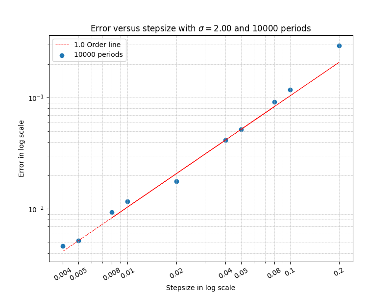
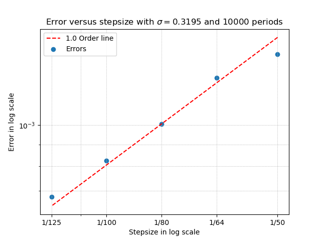
On the other hand, conducting numerical approximation with Euler-Maruyama scheme, we obtain X^s+kโ€‹ฮ”โ€‹ts,xsuperscriptsubscript^๐‘‹๐‘ ๐‘˜ฮ”๐‘ก๐‘ ๐‘ฅ\widehat{X}_{s+k{\Delta t}}^{s,x} for a range of different ${\Delta t}<2/\pi=0.63662$ varying from $0.2$ to $0.004$. We apply the Euler-Maruyama scheme with same length of time of 10000 periods for different step size ${\Delta t}$. The error is presented in Table 1 and as a log-log graph in Figure 1. Our numerical results show very good order 1 line fitting. Note the exact value $\int_{{\mathbb{R}}^{d}}x^{2}\bar{\rho}(d{x})=10.266021$ (rounded off in 6 decimal places).

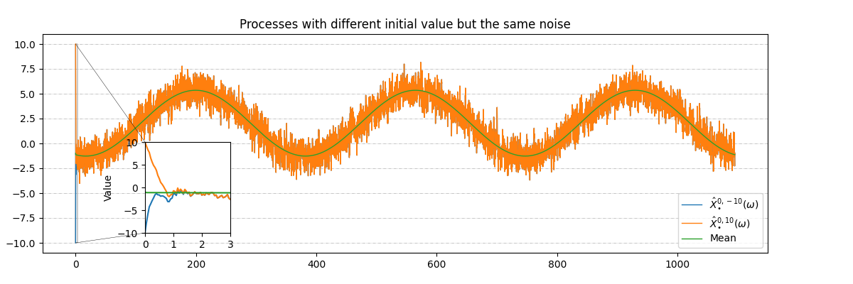
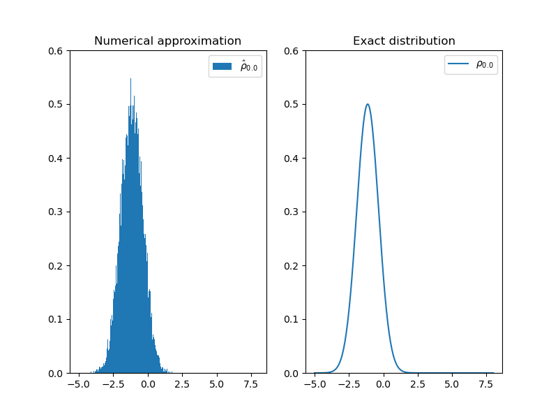
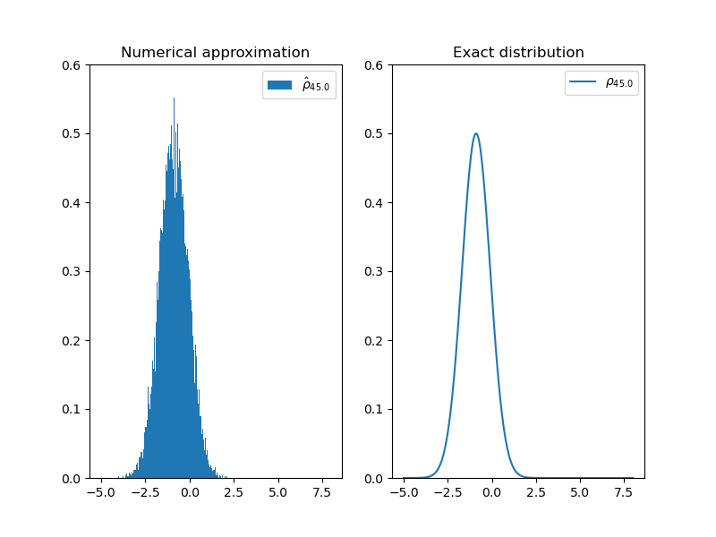
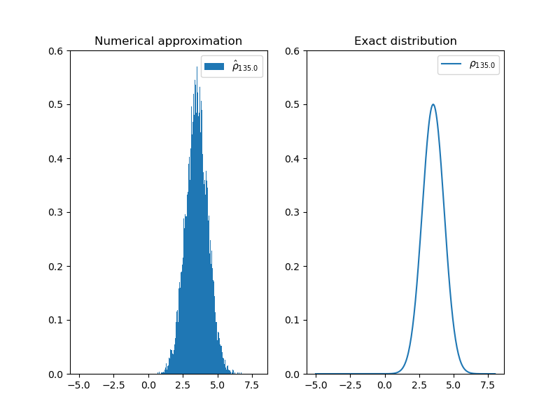
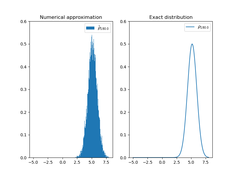
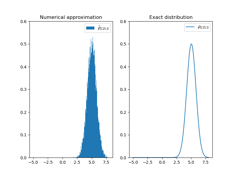
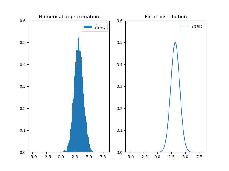
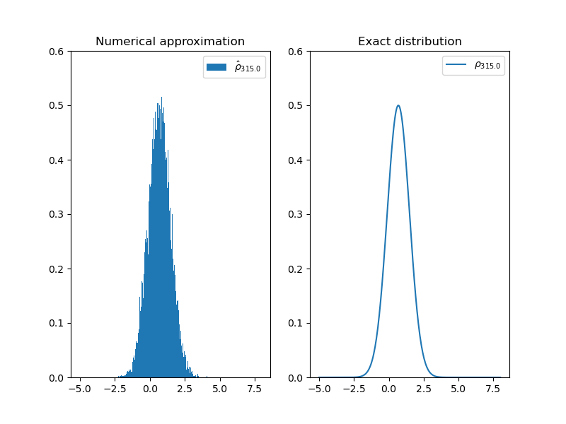
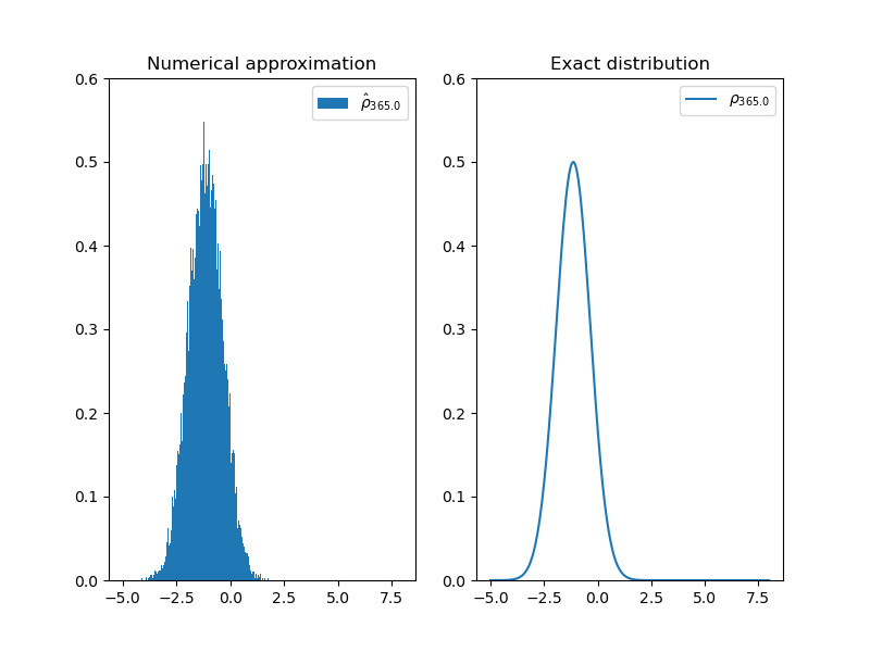
In Figure 2, we present two numerical approximations, X^s0,โˆ’10superscriptsubscript^๐‘‹๐‘ 010\widehat{X}_{s}^{0,-10} and X^s0,10superscriptsubscript^๐‘‹๐‘ 010\widehat{X}_{s}^{0,10}, to random periodic path with different initial values. These two trajectories are generated with the same realisation of noise. They merge before $t=2$ and show inconspicuous difference after that. We then generate one numerical approximation to random periodic path with 10000 periods and step size ${\Delta t}=0.01$. We collect the points on time $t=k\tau$ to build the histogram in left hand side graph of Figure 3(3(a)) compared with its theoretical result $\rho_{0}$. In Figure 3, we give 8 more comparisons between numerical approximations to the periodic measure and its theoretical results.

Step sizes ${\Delta t}=0.2$ ${\Delta t}=0.1$ ${\Delta t}=0.08$ ${\Delta t}=0.05$ ${\Delta t}=0.04$
Approximation 10.560044 10.383899 10.357855 10.318126 10.307453
Numerical error 0.294024 0.117879 0.091834 0.052105 0.041433
CPU(seconds) 175.41 371.39 465.71 756.28 951.37
Step sizes ${\Delta t}=0.02$ ${\Delta t}=0.01$ ${\Delta t}=0.008$ ${\Delta t}=0.005$ ${\Delta t}=0.004$
Approximation 10.283706 10.277765 10.275399 10.271213 10.270654
Numerical error 0.017686 0.011745 0.009379 0.005192 0.004634
CPU(seconds) 1600.47 3711.75 4407.75 6551.42 7600.27
Table 1: Numerical results of Example 6.1 where approximations and numerical errors are rounded off in 6 decimal places
Refer to caption
Figure 1: Error of approximation to the average of periodic measure versus step size in log-log graph (Example 6.1)
Refer to caption
Figure 2: Paths of the temperature model (Example 6.1)
Refer to caption
(a) $\hat{\rho}_{0}$ and $\rho_{0}$
Refer to caption
(b) $\hat{\rho}_{45}$ and $\rho_{45}$
Refer to caption
(c) $\hat{\rho}_{90}$ and $\rho_{90}$
Refer to caption
(d) $\hat{\rho}_{135}$ and $\rho_{135}$
Refer to caption
(e) $\hat{\rho}_{180}$ and $\rho_{180}$
Refer to caption
(f) $\hat{\rho}_{225}$ and $\rho_{225}$
Refer to caption
(g) $\hat{\rho}_{270}$ and $\rho_{270}$
Refer to caption
(h) $\hat{\rho}_{315}$ and $\rho_{315}$
Refer to caption
(i) $\hat{\rho}_{365}$ and $\rho_{365}$
Figure 3: Comparisons between approximation of periodic measure with ${\Delta t}=0.01$ and 10000 periods and its theoretical result (Example 6.1)

In practice, we run the computation with 10 different step sizes simultaneously under โ€multiprocessingโ€ package of Python with 7 cores of CPU. The above results of error analysis took 7600.286 seconds of computing time where the CPU time of each step size is given in Table 1. One can see the majority of time was consumed under the small step sizes such as ${\Delta t}=0.004$ and ${\Delta t}=0.005$.

If necessary, one can split the approximation of random periodic path with small step sizes into several jobs. This works well due to ergodicity and fast convergence to random periodic path under our scheme. We do not need it in Example 6.1 as the computing time is reasonably short. But the possibility to split the computation into several independent jobs plays a crucial role in the case when a model has a large period. For such a problem, we need to consider the long time behaviour of $N\tau$ where both $N$ and $\tau$ are large. We will see that in the following example.

Example 6.2.

We consider Benzi-Parisi-Sutera-Vulpianiโ€™s climate dynamics model given by SDE (1.1) with $b(t,x)=x-x^{3}+A\cos(Bt)$ and $\sigma(x)=\sigma$. The coefficients are chosen as $A=0.12$, $B=0.001$ and $\sigma=0.285$ as discussed in [7] and [15]. We make a time scaling by taking $b(t,x)=0.4\pi(x-x^{3}+0.12\cos(0.0004\pi t))$ and $\sigma(x)=0.285\times\sqrt{0.4\pi}\approx 0.3195$, so the period $\tau=5000$ in the system. Thus when we apply numerical approximation to the model, we can ensure our time step size dividing the period $\tau=5000$. It is also mollified to satisfy the global Lipschitz assumption in this paper. For this, what we could do is to modify the function $x-x^{3}$ by a linear function $128-47x$ when $x\geq 4$ and $-128-47x$ when $x\leq-4$ and smooth this function by mollifier $\eta_{\varepsilon}(x)=\eta(x)$, where ฮทโ€‹(x)={Cโ€‹expโก(1|x|2โˆ’1)|x|โ‰ค10oโ€‹tโ€‹hโ€‹eโ€‹rโ€‹wโ€‹iโ€‹sโ€‹e๐œ‚๐‘ฅcases๐ถ1superscript๐‘ฅ21๐‘ฅ10๐‘œ๐‘กโ„Ž๐‘’๐‘Ÿ๐‘ค๐‘–๐‘ ๐‘’\eta(x)=\begin{cases}C\exp\left(\frac{1}{\left|x\right|^{2}-1}\right)&\left|x\right|\leq 1\\ 0&otherwise\end{cases} and $C$ is chosen such that $\int\eta(x)dx=1$. But this adds a lot of computing time as integration of convolution is needed in every step of the computation.

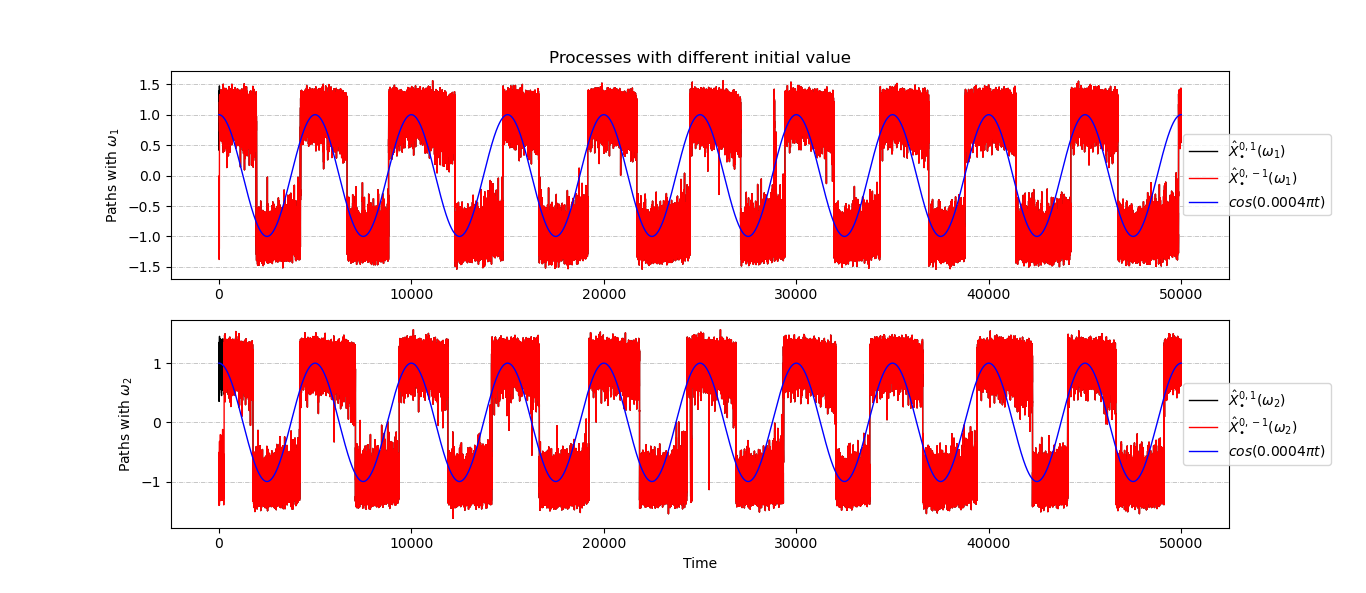
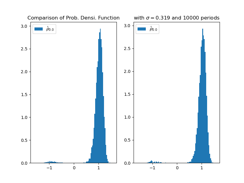
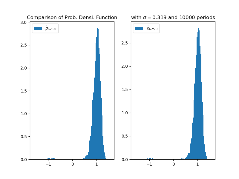
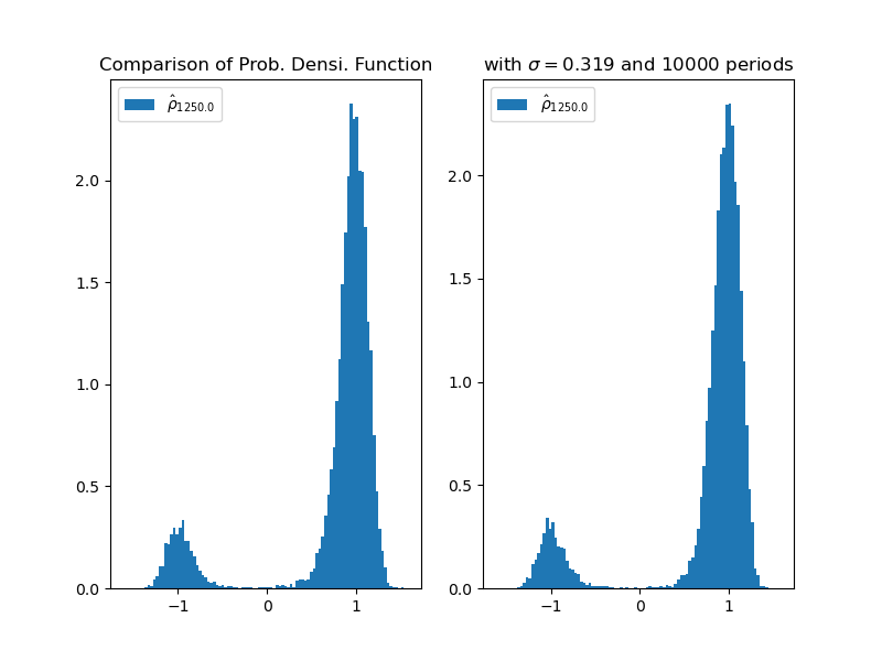
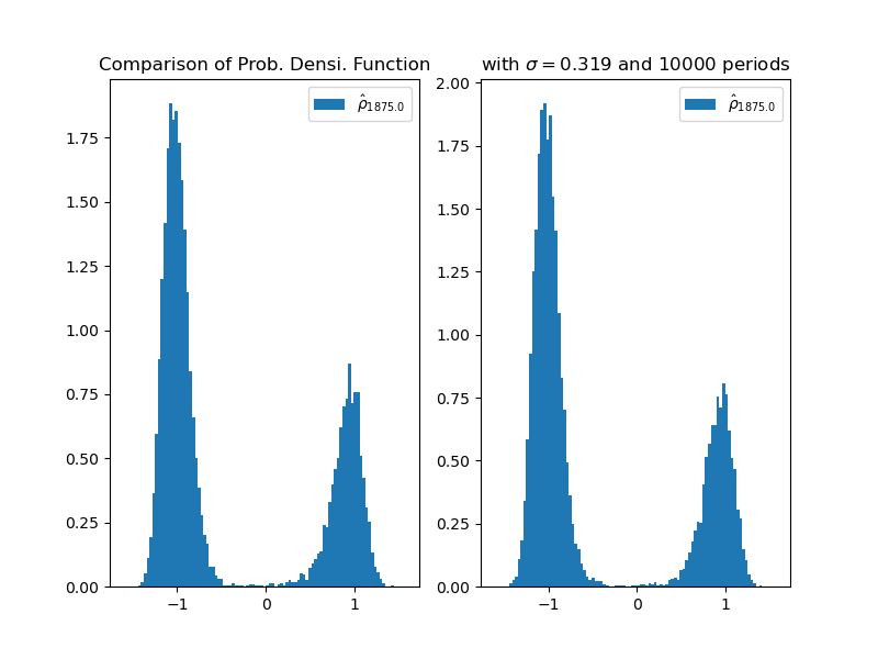
In our approximation, the drift term is $\hat{b}(t,x)=0.4\pi((1-\exp(-\frac{50}{x^{2}}))(x-x^{3})+0.12\cos(0.0004\pi t))$. This function makes a very good approximation to function $b(t,x)$ when $\left|x\right|\leq 4$ though it is not the case globally. Note this function is Lipschitz and smooth. As we mentioned in the introduction, our modified model provides the same climate dynamics as the original one of Benzi-Parisi-Sutera-Vulpiani. Our numerical simulations presented in Figure 5 for the modified equation provide strong evidence that is the case as seen in the Figure 5 that the trajectory rarely goes outside of $[-4,4]$. In fact, during the approximation with 10000 periods, we did not find any point in the whole data set running out of this interval.

Note this model does not have an explicit solution, so we cannot carry out the error analysis as we did in Example 6.1. To overcome this difficulty we use the approximation of solution with ${\Delta t}=0.001$ to replace our exact solution in the error analysis. To make the computation more efficient, we split the approximation involving $\frac{5000\times 10000}{0.001}=5\times 10^{10}$ iterations to 8 individual jobs of $6.25\times 10^{9}$ iterations with independent Brownian motions. The results are shown in the left hand side table of Table 2. We then conduct the numerical experiment for step size varying from $1/125$ to $1/50$. The error is in the right hand side table of Table 2 and the log-log graph is presented in Figure 4. We carry out numerical simulation with 10000 periods for each step size and our total cost is 155547.50 seconds with 7 cores.

We consider numerical simulation with ${\Delta t}=0.01$ to show the stochastic resonance phenomenon in Figure 5. The simulations start from different initial condition but the same realisation of noise in each sub-graph, where one can see the convergence to random periodic path is also very fast. Together with ergodicity, it provides the possibility of splitting 10000 periods into several independent approximations for the step size ${\Delta t}=0.001$. Without the split, our total computing time would be about $5\times 10^{5}$ seconds as 6 cores of CPU are idle for long time.

Result CPU(seconds)
1 1.0120872 71050.63
2 1.0121229 70247.79
3 1.0120366 70782.51
4 1.0121788 70421.53
5 1.0118910 70679.84
6 1.0117187 69755.99
7 1.0115235 67978.79
8 1.0118564 60069.49
Mean value of ${\Delta t}=0.001$ is 1.0119269
Step sizes ${\Delta t}=1/50$ ${\Delta t}=1/64$ ${\Delta t}=1/80$
Approximation 1.0104580 1.0106331 1.0109203
Numerical error 0.0014689 0.0012938 0.0010066
CPU(seconds) 28630.88 36177.61 45509.97
Step sizes ${\Delta t}=1/100$ ${\Delta t}=1/125$
Approximation 1.0111015 1.0112500
Numerical error 0.0008254 0.0006769
CPU(seconds) 56691.58 49771.05
Table 2: Numerical results of Example 6.2 where numerical results and errors are rounded off in 7 decimal places
Refer to caption
Figure 4: Error of approximation to average of periodic measure versus step size in log-log graph (Example 6.2)

We also generate the periodic measure approximations from two paths each with 10000 periods and the step size ${\Delta t}=0.01$ under two different realisations of noise. The distributions of periodic measure are presented in Figure 6. One can see the distributions produced by two different Brownian motions are very similar. There are some minor differences due to insufficient amount of data. If we utilise sufficiently large amount of computations, the differences will eventually disappear.

Refer to caption
Figure 5: Paths of stochastic resonance model (Example 6.2)

We can apply time scaling on the model to rescale its period to a much smaller number. By doing this, the Lipschitz coefficient of the drift term will become very large. According to the upper bound of step size in Theorem 5.1, the total cost of approximation will remain the same as the step size has to be very small.

Acknowledgements

We would like to acknowledge the financial support of an EPSRC grant (ref. EP/S005293/2). We are very grateful to the referees for their constructive comments which led to significant improvements of this paper.

Refer to caption
(a) Distribution of $\hat{\rho}_{0}$
Refer to caption
(b) Distribution of $\hat{\rho}_{625}$
Refer to caption
(c) Distribution of $\hat{\rho}_{1250}$
Refer to caption
(d) Distribution of $\hat{\rho}_{1875}$
Refer to caption
(e) Distribution of $\hat{\rho}_{2500}$
Refer to caption
(f) Distribution of $\hat{\rho}_{3125}$
Refer to caption
(g) Distribution of $\hat{\rho}_{3750}$
Refer to caption
(h) Distribution of $\hat{\rho}_{4375}$
Refer to caption
(i) Distribution of $\hat{\rho}_{5000}$
Figure 6: Approximations of periodic measure with ${\Delta t}=0.01$ and 10000 periods (Example 6.2)

References

  • [1]
  • [2] R. A. Adams, J. J. F. Fournier, Sobolev Spaces, 2nd edn., Academic Press, China, 2009.
  • [3] P. W. Bates, K.N. Lu, B.X. Wang, Attractors of non-autonomous stochastic lattice systems in weighted spaces, Phys. D, 289 (2014), 32-50.
  • [4] F. E. Benth and J. Benth, The volatility of temperature and pricing of weather derivatives, Quantitative Finance, 7(5) (2007), 553-561.
  • [5] R. Benzi, G. Parisi, A. Sutera and A. Vulpiani, Stochastic resonance in climatic change, Tellus, 34 (1982), 10-16.
  • [6] M. D. Chekroun, E. Simonnet, M. Ghil, Stochastic climate dynamics: random attractors and time-dependent invariant measures, Phys. D, 240 (2011), 1685-1700.
  • [7] A. M. Cherubini, J. S. W. Lamb, M. Rasmussen, Y. Sato, A random dynamical systems perspective on stochastic resonance, Nonlinearity, 30 (2017), 2835-2853.
  • [8] M. Engel, C, Kuehn, A random dynamical systems perspective on isochronicity for stochastic oscillations, 2019, arXiv:1911.08993.
  • [9] C. Feng, Y. Liu, H. Zhao, Numerical approximation of random periodic solutions of stochastic differential equations, Z. Angew. Math. Phys., 68 (2017) 119, pp1-32.
  • [10] C.R. Feng, B.Y. Qu and H.Z. Zhao, Random quasi-periodic paths and quasi-periodic measures of stochastic differential equations, J. of Differential Equations, Vol. 286 (2021), 119-163.
  • [11] C. Feng, Y. Wu, H. Zhao, Anticipating random periodic solutionsโ€“I. SDEs with multiplicative linear noise, J. Funct. Anal., 271 (2016), 365-417.
  • [12] C. Feng, H. Zhao, Random periodic solutions of SPDEs via integral equations and Wiener-Sobolev compact embedding, J. Funct. Anal., 262 (2012), 4377-4422.
  • [13] C. Feng, H. Zhao, Random periodic processes, periodic measures and ergodicity, J. of Differential Equations, 269 (2020), 7382-7428.
  • [14] C. Feng, H. Zhao, J. Zhong, Existence of geometric ergodic periodic measures of stochastic differential equations, Preprint, 2019, arXiv:1904.08091.
  • [15] C. Feng, H. Zhao, J. Zhong, Expected exit time for time-periodic stochastic differential equations and applications to stochastic resonance, Physica D, 417 (2021) 132815, pp. 1-18.
  • [16] C. Feng, H. Zhao, B. Zhou, Pathwise random periodic solutions of stochastic differential equations, J. Differential Equations, 251 (2011), 119-149.
  • [17] A. Grorud, D. Talay Approximation of Lyapunov exponents of nonlinear stochastic differential equations, SIAM J. Appl. Math, 56 (1996), 627-650.
  • [18] D. Higham, X. Mao, A. Stuart, Exponential mean-square stability of numerical solutions to stochastic differential equations, LMS J. Comput. Math., 6 (2003), 297-313.
  • [19] R. Hรถpfner, E. Lรถcherbach, M. Thieullen, Strongly degenerate time inhomogeneous SDEs: densities and support properties. Application to a Hodgkin-Huxley system with periodic input. Bernoulli, 23 (2017), 2587-2616.
  • [20] W. Huang, Z. Lian, K. Lu, Ergodic theory of random Anosov systems mixing on fibers, 2019, arXiv:1612.08394.
  • [21] A. Jentzen, P. Kloeden, Taylor expansions of solutions of stochastic partial differential equations with additive noise, Ann. Probab., 38 (2010), 532-569.
  • [22] P. E. Kloeden, E. Platen, Numerical Solution of Stochastic Differential Equations, Springer-Verlag, New York, 1991.
  • [23] H. Kunita, Stochastic differential equations and stochastic flows of diffeomorphisms, Ecole dโ€™รฉtรฉ de Probabilitรฉs de Saint-Flour XII-1982, Lecture Notes in Mathematics, Springer, 1984.
  • [24] J. Mattingly, A.M. Stuart, D.J. Higham, Ergodicity for SDEs and approximations: locally Lipschitz vector fields and degenerate noise, Stochastic Process. Appl., 101 (2002), 185-232.
  • [25] S. P. Meyn, R. L. Tweedie, Markov Chains and Stochastic Stability, Springer-Verlag, 1993.
  • [26] G. N. Milstein, Numerical Integrations of Stochastic Differential Equations, Kluwer, 1995.
  • [27] G. N. Milstein, M. V. Tretyakov, Stochastic Numerics for Mathematical Physics, Springer, 2004.
  • [28] E. Nummelin, General irreducible Markov chains and non-negative operators, Cambridge University Press, 1984.
  • [29] D. Talay, Second order discretization schemes of stochastic differential systems for the computation of the invariant law, Stoch. Stoch. Rep., 29 (1990), 13-36.
  • [30] D. Talay, Approximation of upper Lyapunov exponents of bilinear stochastic differential systems, SIAM J. Numer. Anal., 28 (1991), 1141-1164.
  • [31] D. Talay, L.Rubaro, Expansion of the global error for numerical schemes solving stochastic differential equations, Stoch. Anal. Appl., 8 (1990), 483-509.
  • [32] A. Tocino, R. Ardanuy, Runge-Kutta methods for numerical solution of stochastic differential equations, J. Comput. Appl. Math., 138 (2002), 219-241.
  • [33] B.X. Wang, Existence, stability and bifurcation of random complete and periodic solutions of stochastic parabolic equations, Nonlinear Anal., 103 (2014), 9-25.
  • [34] A. Yevik, H. Zhao, Numerical approximations to the stationary solutions of stochastic differential equations, SIAM J. Numer. Anal., 49 (2011), 1397-1416.
  • [35] C. Yuan, X. Mao, Stability in distribution of numerical solutions for stochastic differential equations, Stoch. Anal. Appl., 22 (2004), 1133-1150.
  • [36] H. Zhao, Z. Zheng, Random periodic solutions of random dynamical systems, J. Differential Equations, 246 (2009), 2020-2038.