Bounded support in linear random coefficient models: Identification and variable selection

Abstract

We consider linear random coefficient regression models, where the regressors are allowed to have a finite support. First, we investigate identifiability, and show that the means and the variances and covariances of the random coefficients are identified from the first two conditional moments of the response given the covariates if the support of the covariates, excluding the intercept, contains a Cartesian product with at least three points in each coordinate. We also discuss ientification of higher-order mixed moments, as well as partial identification in the presence of a binary regressor. Next we show the variable selection consistency of the adaptive LASSO for the variances and covariances of the random coefficients in finite and moderately high dimensions. This implies that the estimated covariance matrix will actually be positive semidefinite and hence a valid covariance matrix, in contrast to the estimate arising from a simple least squares fit. We illustrate the proposed method in a simulation study.

Keywords. Adaptive LASSO, random coefficient regression model, random effects, variable selection

1 Introduction

In various statistical analyses in fields such as medicine and economics, there is a large extent of individual heterogeneity in the effect of observed covariates, which is routinely modeled by random coefficients - also called random effects - models. For example, in contemporary microeconomic data sets with many observations and potentially a large number of explanatory variables, non-observed heterogeneity plays an important role (Lewbel, 2005). An important issue then is to select those coefficients which actually are random if there is a large set of potential variables which might have individual - specific effects.

To this end, in this paper we shall consider the following random coefficients regression model

$$Y=B_{0}+{\mathbf{W^{\top}}}{\mathbf{B}}\,,$$ (1)

where ${\mathbf{B}},{\mathbf{W}}\in{\mathbb{R}}^{p-1}$ are independent random vectors, $B_{0}$ is a random variable and ${\mathbf{W}}=(W_{1},\dotsc,W_{p-1})^{\top}$ represents the random regressors.

Model (1), which is related to random effects models from the literature on biostatistics (Schelldorfer et al., 2011), was introduced by Hildreth and Houck (1968) and Swamy (1970). They assumed that $B_{0},\ldots,B_{p-1}$ are independent, and focused on estimating their means and variances by least squares in two stages. Arellano and Bonhomme (2012) studied a panel - version of the random coefficient model. Beran and Hall (1992) initiated the nonparametric analysis of the distribution of the random coefficients. For $p=2$, Beran et al. (1996) used Fourier methods to construct an estimator of the joint density of $(B_{0},B_{1})^{\top}$. Their method was taken up again by Hoderlein et al. (2010), who put it into the form of a more conventional kernel estimator and generalized it to arbitrary dimension $p$. Further related literature includes Gautier and Kitamura (2013), who analyze a binary choice version of the model, Lewbel and Pendakur (2017) who study a generalization of (1) in which the products $B_{1}\,W_{1},\ldots,B_{p-1}\,W_{p-1}$ are related to $Y$ by some arbitrary (possibly non-linear) unknown function, as well as Hoderlein et al. (2017), Breunig and Hoderlein (2018), Dunker et al. (2019) and Holzmann and Meister (2020). Recently, Gaillac and Gautier (2021) studied nonparametric identification and adaptive estimation in a random coefficient regression model, where covariates have bounded but continuous variation.

The above nonparametric approaches which target the full density of the random coefficients require a large or at least, as in Gaillac and Gautier (2021), continuous support of the covariates, which is often an unrealistic assumption in applications. In this paper, we shall focus on situations in which the covariates have bounded and in particular finite support. In this latter setting there is little hope to identify and estimate the density of the random coefficients nonparametrically. Therefore, we shall focus on the first and second moments, which are arguably of most interest in applications. Variable selection techniques for means, variances and covariances of the random coefficients then allow to determine which variables have an effect on average (non-zero mean of the coefficient), which variables have heterogenous effects (non-zero variances) and for which covariates the effects are correlated. In particular, we shall argue that it is important not to focus exclusively on the variances of the random coefficients, but to take the full variance-covariance matrix into account. Further, estimating the first and second moments of the random coefficients then allows to predict the first and second moments of the response $Y$ conditional on the covariates. Finally, normality of the random coefficients is a common parametric assumption, under which their distribution is fully determined by means, variances and covariances.

Model (1) is related to random effects models from the literature on biostatistics (Schelldorfer et al., 2011). These are studied in a longitudinal framework, and the goal is then to estimate the fixed effects by using a quasi-likelihood approach and to predict the random effects. Papers which study these models in a high-dimensional setting are, among others, Schelldorfer et al. (2011) and Li et al. (2021).

The paper is organized as follows. In Section 2 we clarify under which assumptions on the support of the covariates, first and second moments of the random coefficients are identified. It turns out that identification holds if the support of the covariate vector contains a Cartesian product with at least three support points for each covariate. Conversely, identification generally fails if one covariate only has two support points. In Section 3 we turn to estimation and in particular to variable selection with a focus on the variances and covariances in model (1). We use the adaptive LASSO originally introduced in Zou (2006a), which may achieve variable selection consistency without additional restrictive assumptions such as the irrepresentable assumption required for the ordinary LASSO, and show the variable selection consistency in fixed and moderately high dimensions. The technical issues are to deal with the residuals when estimating centered second moments of the random coefficients as well as with the heteroscedasticity of the model.] Section 4 contains some numerical illustrations. Proofs of the main results are given in Section 5, while some further auxiliary results are deferred to the supplementary appendix.

We shall use the following notation: For an $n\times p$ matrix $\mathbb{X}$ and a subset $S\subseteq\{1,\ldots,p\}$ of the index set, $\mathbb{X}_{S}$ denotes the $n\times|S|$ matrix containing those columns of $\mathbb{X}$ with indices in $S$. A similar notation is $\boldsymbol{v}_{S}$ for a vector $\boldsymbol{v}\in{\mathbb{R}}^{p}$. ${\left\lVert\mathbb{X}\right\rVert_{\mathrm{M},2}}$ denotes the operator norm of $\mathbb{X}$ for the Euclidean norm, and ${\left\lVert\mathbb{X}\right\rVert_{\mathrm{F}}}$ the Frobenius norm, that is the Euclidean norm of the vectorization of $\mathbb{X}$.

2 Identification of first and second moments

In model (1) we also write ${\mathbf{A}}=(B_{0},{\mathbf{B^{\top}}})^{\top}\in{\mathbb{R}}^{p}$, so that ${\mathbf{A}}=(A_{1},\dotsc,A_{p})^{\top}$ and ${\mathbf{W}}$ are independent. We assume that the first and second moments of the random coefficients ${\mathbf{A}}$ exist and set

$$\mu^{*}\mathrel{\vbox{\hbox{\scriptsize.}\hbox{\scriptsize.}}}={\mathbb{E}}[{\mathbf{A}}]\quad\in{\mathbb{R}}^{p}\,,\qquad\text{and}\qquad\Sigma^{*}\mathrel{\vbox{\hbox{\scriptsize.}\hbox{\scriptsize.}}}={\operatorname{\mathbb{C}\mathrm{ov}}}({\mathbf{A}})={\mathbb{E}}\big{[}({\mathbf{A}}-\mu^{*})({\mathbf{A}}-\mu^{*})^{\top}]\quad\in{\mathbb{R}}^{p\times p}\,.$$ (2)

In this section we consider conditions for identification and partial identification of the moments $\mu^{*}$ and $\Sigma^{*}$ in terms of the support of the covariates ${\mathbf{W}}$.

While one may argue that means and variances are of main applied interest, the joint variation of the random coefficients as described by the covariances and the correlations is also relevant. Further, we shall see that excluding covariances from the analysis and falsely assuming a diagonal covariance matrix a-priori can lead to wrong conclusions about the (non-)randomness of the coefficients. The proofs of the results in this section are collected in Section 5.1.

To illustrate, first consider the case of a single regressor, resulting in the model

$$Y=B_{0}+W_{1}\,B_{1}\,.$$ (3)

For $W_{1}$ supported on $\{0,1\}$ we have the following result.

Proposition 1.

Suppose that in model (3) the random variable $W_{1}\in\{0,1\}$ is binary, and denote the identified standard deviations by

$$s_{1}=\sqrt{{\operatorname{\mathbb{V}\mathrm{ar}}}(B_{0})}\,,\qquad s_{2}=\sqrt{{\operatorname{\mathbb{V}\mathrm{ar}}}(B_{0}+B_{1})}\,.$$

Then each value

$$\sqrt{{\operatorname{\mathbb{V}\mathrm{ar}}}(B_{1})}\in\big{[}|s_{1}-s_{2}|,s_{1}+s_{2}\big{]}$$

is consistent with $s_{1}$ and $s_{2}$, provided the correlation $\rho={\operatorname{\mathbb{C}\mathrm{or}}}(B_{0},B_{1})$ is chosen for $\sqrt{{\operatorname{\mathbb{V}\mathrm{ar}}}(B_{1})}>0$ as

$$\rho=\frac{s_{2}^{2}-s_{1}^{2}-{\operatorname{\mathbb{V}\mathrm{ar}}}(B_{1})}{2\,s_{1}\sqrt{{\operatorname{\mathbb{V}\mathrm{ar}}}(B_{1})}}\in\begin{cases}[-1,1],&\text{if }s_{2}>s_{1}\,,\\ \big{[}-1,-\sqrt{s_{1}^{2}-s_{2}^{2}}/s_{1}\big{]}&\text{if }s_{1}\geq s_{2}\,.\end{cases}$$ (4)

Thus, to conclude from ${\operatorname{\mathbb{V}\mathrm{ar}}}(B_{0})={\operatorname{\mathbb{V}\mathrm{ar}}}(B_{0}+B_{1})$ that ${\operatorname{\mathbb{V}\mathrm{ar}}}(B_{1})=0$ fully relies on the assumption of a diagonal covariance matrix, without this assumption, $B_{1}$ can well be random.

On the other hand, the following proposition shows that three distinct support points of $W_{1}$ are enough to identify the means ${\mathbb{E}}[B_{j}]$, the variances ${\operatorname{\mathbb{V}\mathrm{ar}}}(B_{j})$, $j=0,1$, and the covariance ${\operatorname{\mathbb{C}\mathrm{ov}}}(B_{0},B_{1})$. From Proposition 1 and not surprisingly, two support points are insufficient for this purpose.

Proposition 2.

In model (3), if $W_{1}$ has $n+1$ support points and ${\mathbb{E}}\big{[}|B_{0}|^{n}\big{]},{\mathbb{E}}\big{[}|B_{1}|^{n}\big{]}<\infty$, then all mixed moments ${\mathbb{E}}\big{[}B_{0}^{j}\,B_{1}^{k}\big{]}$, $j,k\geq 0$, $j+k\leq n$, are identified.

2.1 Identification of the covariance matrix

Now let us turn to the identification of $\mu^{*}$ and $\Sigma^{*}$ in (2) in general dimensions. To this end, consider the half-vectorization of symmetric matrices of dimension $p\times p$,

$${\operatorname{vec}}(M)=\big{(}M_{11},\dotsc,M_{pp},M_{12},\dotsc,M_{1p},M_{23},\dotsc,M_{2p},\dotsc,M_{(p-1)p}\big{)}^{\top}\in{\mathbb{R}}^{\frac{p(p+1)}{2}}$$ (5)

for $M\in{\mathbb{R}}^{p\times p}$ with $M^{\top}=M$, and set

$$\sigma^{*}\mathrel{\vbox{\hbox{\scriptsize.}\hbox{\scriptsize.}}}={\operatorname{vec}}(\Sigma^{*}).$$

Note that the first $p$ entries of $\sigma^{*}$ are the variances and the remaining entries are the covariances. In model (1) we have that

$${\operatorname{\mathbb{V}\mathrm{ar}}}\,\big{(}Y\,\big{|}\,{\mathbf{W}}={\mathbf{w}})=(1,{\mathbf{w^{\top}}})\,\Sigma^{*}\,(1,{\mathbf{w^{\top}}})^{\top},$$ (6)

so that the quadratic form in $\Sigma^{*}$ is identified over $(1,{\mathbf{w}})$ with ${\mathbf{w}}$ ranging over the support of ${\mathbf{W}}$. Note that (6) can be written in vectorized form as

$${\operatorname{\mathbb{V}\mathrm{ar}}}\,\big{(}Y\,\big{|}\,{\mathbf{W}}={\mathbf{w}}) =\big{(}1,({\mathbf{w}}^{2})^{\top},2{\mathbf{w^{\top}}},2w_{1}w_{2},\dotsc,2w_{1}w_{p-1},2w_{2}w_{3},\dotsc,2w_{p-2}w_{p-1}\big{)}\,\sigma^{*}\,$$

$$={\operatorname{v}}\big{(}(1,{\mathbf{w^{\top}}})^{\top}\big{)}^{\top}\,\sigma^{*}\,,$$ (7)

where we recall that $\sigma^{*}={\operatorname{vec}}(\Sigma^{*})$, and the vector transformation ${\operatorname{v}}$ is defined by

$${\operatorname{v}}({\mathbf{x}})=\big{(}x_{1}^{2},\dotsc,x_{p}^{2},2x_{1}x_{2},\dotsc,2x_{1}x_{p},2x_{2}x_{3},\dotsc,2x_{2}x_{p},\dotsc,2x_{p-1}x_{p}\big{)}^{\top}\in{\mathbb{R}}^{\frac{p(p+1)}{2}}\,,\quad{\mathbf{x}}\in{\mathbb{R}}^{p}.$$ (8)

Based on (2.1) we can establish linear equations for the $p(p+1)/2$ entries of $\Sigma^{*}$ respectively $\sigma^{*}$. With the above notation, we may state the following basic result.

Theorem 3.

In model (1) a sufficient condition for identification of the mean vector $\mu^{*}$ and the covariance matrix $\Sigma^{*}$ is the existence of $p(p+1)/2$ points ${\mathbf{w_{1}}},\dotsc,{\mathbf{w_{p(p+1)/2}}}\in{\mathbb{R}}^{p-1}$ in the support of ${\mathbf{W}}$, for which the matrix

$$S=\bigg{[}{\operatorname{v}}\Big{(}(1,{\mathbf{w_{1}^{\top}}})^{\top}\Big{)},\dotsc,{\operatorname{v}}\Big{(}(1,{\mathbf{w_{p(p+1)/2}^{\top}}})^{\top}\Big{)}\bigg{]}^{\top}$$ (9)

of dimension $p(p+1)/2\times p(p+1)/2$ is of full rank. This condition is also necessary for identification in the subset of full-rank covariance matrices.

The theorem remains valid if one can show that for $m\geq p(p+1)/2$ support points, the resulting matrix $S_{m}$ has full rank $p(p+1)/2$. In the following example, we show that the condition of the previous theorem can never be satisfied if one of the regressors only has two support points.

Example 1.

Suppose that $W_{1}$ has only two support points $a$ and $b$ and that the joint support of ${\mathbf{W}}$ is finite. Then the matrix $S_{m}$, where $m$ is the total number of support points, has rank at most $p(p+1)/2-1$. Thus, from Theorem 3, full-rank covariance matrices $\Sigma^{*}$ are not identified. Indeed, the matrix $S_{m}^{\top}$ contains the submatrix

$$\begin{bmatrix}1&\dotsc&1&1&\dotsc&1\\ a^{2}&\dotsc&a^{2}&b^{2}&\dotsc&b^{2}\\ 2a&\dotsc&2a&2b&\dotsc&2b\end{bmatrix}\quad\in{\mathbb{R}}^{3\times m}\,.$$

Evidently, this matrix is of column rank at most $2$, since there are only two distinct columns. Thus, its row rank is also at most two, which implies that the corresponding three columns in $S_{m}$ are linearly dependent.

In contrast, if each covariate has at least three support points and the joint support contains the corresponding Cartesian product, then we retain identification of $\Sigma^{*}$.

Theorem 4.

Consider model (1). Suppose that the support of ${\mathbf{W}}=(W_{1},\dotsc,W_{p-1})^{\top}$ contains the Cartesian product of three points in each coordinate. Then there exist $p(p+1)/2$ support points such that the matrix $S$ in (9) has full rank $p(p+1)/2$ and consequently, the means and (co-)variances of the random coefficients ${\mathbf{A}}$ are identified. Conversely, if there is a $W_{j}$ having only two support points, then in the full-rank covariance matrices identification fails.

2.2 Partial identification

What can be said about the covariance matrix of the random coefficients if there are binary regressors? Assume a single binary regressor $Z$, and additional regressors ${\mathbf{W}}\in{\mathbb{R}}^{p-2}$ (slightly modifying the notation in this section) for which the support contains a Cartesian product with at least three points in each coordinate. Our model is then written as

$$Y=B_{0}+Z\,B_{1}+{\mathbf{W^{\top}}}{\mathbf{B_{2}}}\,.$$

The set of covariance matrices of ${\mathbf{A}}=(B_{0},B_{1},{\mathbf{B_{2}^{\top}}})^{\top}\in{\mathbb{R}}^{p}$ consistent with the conditional second moments of $Y$ is

$$\begin{split}\mathcal{S}\mathrel{\vbox{\hbox{\scriptsize.}\hbox{\scriptsize.}}}=&\big{\{}\Sigma\in{\mathbb{R}}^{p\times p}\,\big{|}\,\Sigma\text{ positive semi-definite and}\\ &\quad\quad(1,z,{\mathbf{w^{\top}}})\,\Sigma\,(1,z,{\mathbf{w^{\top}}})^{\top}={\operatorname{\mathbb{V}\mathrm{ar}}}(Y\,|\,Z=z,{\mathbf{W}}={\mathbf{w}})\ \forall\ (z,{\mathbf{w}})\in\text{supp}(Z,{\mathbf{W}})\big{\}}\,.\end{split}$$ (10)

Suppose that the support of $(Z,{\mathbf{W^{\top}}})^{\top}\in{\mathbb{R}}^{p-1}$ has a product structure. From Theorem 4, using $Z=0$ and $Z=1$ we identify the covariance matrices

$${\operatorname{\mathbb{C}\mathrm{ov}}}\big{(}(B_{0},{\mathbf{B_{2}^{\top}}})^{\top}\big{)}\quad\text{and}\quad{\operatorname{\mathbb{C}\mathrm{ov}}}\big{(}(B_{0}+B_{1},{\mathbf{B_{2}^{\top}}})^{\top}\big{)}\,,$$

or equivalently

$${\operatorname{\mathbb{C}\mathrm{ov}}}\big{(}(B_{0},{\mathbf{B_{2}^{\top}}})^{\top}\big{)}\,,\qquad{\operatorname{\mathbb{C}\mathrm{ov}}}\big{(}B_{1};{\mathbf{B_{2}}}\big{)}\,,\qquad{\operatorname{\mathbb{V}\mathrm{ar}}}(B_{0}+B_{1})\,.$$ (11)

Here for random vectors ${\mathbf{C}}$ and ${\mathbf{D}}$, ${\operatorname{\mathbb{C}\mathrm{ov}}}({\mathbf{C}})$ is the covariance matrix of ${\mathbf{C}}$, while ${\operatorname{\mathbb{C}\mathrm{ov}}}({\mathbf{C}};{\mathbf{D}})$ contains the cross-covariances of ${\mathbf{C}}$ and ${\mathbf{D}}$. Sharp bounds for ${\operatorname{\mathbb{V}\mathrm{ar}}}(B_{1})$ are given by

$$\inf_{\Sigma\in\mathcal{S}}\Sigma_{22}\leq{\operatorname{\mathbb{V}\mathrm{ar}}}(B_{1})\,\leq\sup_{\Sigma\in\mathcal{S}}\Sigma_{22}\,,$$ (12)

where the set $\mathcal{S}$ in (10) is characterized by the restrictions given by the identified parts (11) of the matrix $\Sigma^{*}$. These bounds can be obtained numerically by semi-definite programming. An interesting particular question is the potential randomness of $B_{1}$, which is addressed in the following proposition, which relies on the identified quantities in (11).

Proposition 5.

Suppose that the support of $(Z,{\mathbf{W^{\top}}})^{\top}$ has a product structure, and that only $Z$ is binary.

1. If ${\operatorname{\mathbb{V}\mathrm{ar}}}(B_{0})\not={\operatorname{\mathbb{V}\mathrm{ar}}}(B_{0}+B_{1})$, or if ${\operatorname{\mathbb{C}\mathrm{ov}}}(B_{1};{\mathbf{B_{2}}})$ is not the zero vector, then ${\operatorname{\mathbb{V}\mathrm{ar}}}(B_{1})>0$.

2. Conversely, suppose that ${\operatorname{\mathbb{V}\mathrm{ar}}}(B_{0})={\operatorname{\mathbb{V}\mathrm{ar}}}(B_{0}+B_{1})$ and that ${\operatorname{\mathbb{C}\mathrm{ov}}}(B_{1};{\mathbf{B_{2}}})={\mathbf{0}}_{p-2}$.

   1. If ${\operatorname{\mathbb{C}\mathrm{ov}}}\big{(}(B_{0},{\mathbf{B_{2}^{\top}}})^{\top}\big{)}$ is degenerate, and its kernel contains a vector with non-zero first coordinate, then necessarily ${\operatorname{\mathbb{V}\mathrm{ar}}}(B_{1})=0$.

   2. On the other hand, if ${\operatorname{\mathbb{C}\mathrm{ov}}}\big{(}(B_{0},{\mathbf{B_{2}^{\top}}})^{\top}\big{)}$ has full rank, then the upper bound in (12) for ${\operatorname{\mathbb{V}\mathrm{ar}}}(B_{1})$ is strictly positive.

2.3 Identification of higher-order moments

The $k^{\text{th}}$ -order mixed moments of the random vector ${\mathbf{A}}$, $k\in{\mathbb{N}}$, are given by

$$m(k_{1},\ldots,k_{p})={\mathbb{E}}\big{[}A_{1}^{k_{1}}\,\ldots\,A_{p}^{k_{p}}\big{]},\qquad k_{j}\in{\mathbb{N}}_{0},\ k_{1}+\ldots+k_{p}=k,$$

of which there are $\binom{p+k-1}{k}$ many. Information on the mixed moments in the linear random coefficient model $Y=A_{1}+A_{2}\,W_{1}+\ldots+A_{p}\,W_{p-1}$ comes from the identified conditional $k^{\text{th}}$ moments of $Y$ given ${\mathbf{W}}$,

$${\mathbb{E}}[Y^{k}|{\mathbf{W}}={\mathbf{w}}]={\mathbb{E}}\big{[}\big{(}(1,{\mathbf{w}}^{\top})\,{\mathbf{A}}\big{)}^{k}\big{]}.$$ (13)

These can be represented as an inner product of $\binom{p+k-1}{k}$ - dimensional vectors, one consisting of the mixed moments $m(k_{1},\ldots,k_{p})$, the other with corresponding entry

$$\binom{k}{k_{1}\,\ldots\,k_{p}}\,w_{1}^{k_{2}}\,\cdot\ldots\cdot w_{p-1}^{k_{p}},$$ (14)

where ${\mathbf{w}}=(w_{1},\ldots,w_{p-1})$. Hence, we have analogously to the result in Theorem 3 that if there are $\binom{p+k-1}{k}$ support points ${\mathbf{w}}_{j}$ of ${\mathbf{W}}$ such that if we form the matrix with rows as in (14) for the coordinates of the ${\mathbf{w}}_{j}$, the resulting quadratic matrix has full rank, then the $k^{\text{th}}$ -order mixed moments of ${\mathbf{A}}$ are identified.

While we were not able to obtain a sufficient condition along the lines of Theorem 4, we have the following result which guarantees identification.

Theorem 6.

If in model (1), the support of ${\mathbf{W}}=(W_{1},\dotsc,W_{p-1})^{\top}$ contains $p$ points ${\mathbf{w}}_{1},\ldots,{\mathbf{w}}_{p}$ in general position, for which for each $j\in\{1,\ldots,k\}$ and $i_{1},\ldots,i_{j}\in\{1,\ldots,p\}$, the vector $({\mathbf{w}}_{i_{1}}+\ldots+{\mathbf{w}}_{i_{j}})/j$ is also in the support of ${\mathbf{W}}$. Then the mixed moments of ${\mathbf{A}}$ up to order $k$ are identified.

3 Sign-consistency of the adaptive LASSO estimator

In this section we derive the asymptotic variable selection properties of the adaptive LASSO in the linear random coefficient regression model (1), where we focus on estimating and selecting the variances and covariances of the random coefficients. First, in Section 3.1 we consider an asymptotic regime with a fixed number $p$ of regressors, before turning to the moderately high-dimensional setting in which $p\to\infty$ but at a slower rate than the sample size $n$.

The adaptive LASSO and its variable selection properties, originally introduced in Zou (2006a), have already been investigated intensively in the literature. For example, Zou and Zhang (2009) consider the adaptive LASSO and an adaptive version of the elestic net in moderately high dimensions, while Huang et al. (2008) investigate the high-dimensional situation with strong assumptions on the first stage estimator, and Wagener and Dette (2013) extend their approach to a heteroscedastic framework. Here, our contributions mainly are to deal with the residuals when estimating centered second moments of the random coefficients, and to extend the analysis of Zou and Zhang (2009) to our setting with random coefficients.

We observe independent random vectors $(Y_{1},{\mathbf{W_{1}^{\top}}})^{\top},\dotsc,(Y_{n},{\mathbf{W_{n}^{\top}}})^{\top}$ distributed according to the random coefficient regression model (1), and write

$$Y_{i}=B_{i,0}+{\mathbf{W_{i}^{\top}}}{\mathbf{B_{i}}}={\mathbf{X_{i}^{\top}}}{\mathbf{A_{i}}}\,,\quad i=1,\dotsc,n\,,$$

where ${\mathbf{X_{i}}}=(1,{\mathbf{W_{i}^{\top}}})^{\top}\in{\mathbb{R}}^{p}$ with ${\mathbf{W_{i}}}\sim{\mathbf{W}}$ and ${\mathbf{A_{i}}}=(B_{i,0},{\mathbf{B_{i}^{\top}}})^{\top}\sim{\mathbf{A}}$ are independent random vectors. Here ${\mathbf{X_{i}}}=(X_{i,1},\dotsc,X_{i,p})^{\top}$ represents the observed covariates and ${\mathbf{A_{i}}}=(A_{i,1},\dotsc,A_{i,p})^{\top}$ the unobserved individual regression coefficients.

In the following we denote by

$$S_{\sigma} \mathrel{\vbox{\hbox{\scriptsize.}\hbox{\scriptsize.}}}={\operatorname{supp}}\big{(}\sigma^{*}\big{)}=\Big{\{}k\in\big{\{}1,\dotsc,p(p+1)/2\big{\}}\,\big{|}\,\sigma^{*}_{k}\neq 0\Big{\}}\,,\qquad s_{\sigma}\mathrel{\vbox{\hbox{\scriptsize.}\hbox{\scriptsize.}}}=|S_{\sigma}|\,,$$

the support of the half-vectorization $\sigma^{*}$ of the covariance matrix $\Sigma^{*}$. $S_{\sigma}^{c}\mathrel{\vbox{\hbox{\scriptsize.}\hbox{\scriptsize.}}}=\big{\{}1,\dotsc,p(p+1)/2\big{\}}\setminus S_{\sigma}$ will denote the relative complement of this set.

For an estimator $\widehat{\mu}_{n}$ of $\mu^{*}$ we define the regression residuals $\widetilde{Y}_{i}\mathrel{\vbox{\hbox{\scriptsize.}\hbox{\scriptsize.}}}=Y_{i}-{\mathbf{X_{i}^{\top}}}\widehat{\mu}_{n}$, and write the squared residuals as

$$Y_{i}^{\sigma}\mathrel{\vbox{\hbox{\scriptsize.}\hbox{\scriptsize.}}}=\widetilde{Y}_{i}^{2}={\mathbf{X_{i}^{\top}}}\big{(}D_{i}-\Sigma^{*}+E_{n}+F_{n,i}\big{)}{\mathbf{X_{i}}}\,,$$

where we set

$$D_{i} \mathrel{\vbox{\hbox{\scriptsize.}\hbox{\scriptsize.}}}=\big{(}{\mathbf{A_{i}}}-\mu^{*}\big{)}\big{(}{\mathbf{A_{i}}}-\mu^{*}\big{)}^{\top},\qquad E_{n}\mathrel{\vbox{\hbox{\scriptsize.}\hbox{\scriptsize.}}}=\big{(}\mu^{*}-\widehat{\mu}_{n}\big{)}\big{(}\mu^{*}-\widehat{\mu}_{n}\big{)}^{\top},$$ (15)

$$F_{n,i} \mathrel{\vbox{\hbox{\scriptsize.}\hbox{\scriptsize.}}}=\big{(}{\mathbf{A_{i}}}-\mu^{*}\big{)}\big{(}\mu^{*}-\widehat{\mu}_{n}\big{)}^{\top}+\big{(}\mu^{*}-\widehat{\mu}_{n}\big{)}\big{(}{\mathbf{A_{i}}}-\mu^{*}\big{)}^{\top}.$$ (16)

Applying the half-vectorization ${\operatorname{vec}}$ for symmetric matrices in (5) and the corresponding vector transformation ${\operatorname{v}}$ in (8) we obtain in vector-matrix form

$${{\mathbb{Y}}_{n}^{\sigma}}={{\mathbb{X}}_{n}^{\sigma}}\,\sigma^{*}+{\varepsilon_{n}^{\sigma}}={{\mathbb{X}}_{n,S_{\sigma}}^{\sigma}}\,\sigma_{S_{\sigma}}^{*}+{\varepsilon_{n}^{\sigma}}\,,$$

where

$${{\mathbb{Y}}_{n}^{\sigma}} \mathrel{\vbox{\hbox{\scriptsize.}\hbox{\scriptsize.}}}=\Big{(}\big{(}Y_{1}-{\mathbf{X_{1}^{\top}}}\widehat{\mu}_{n}\big{)}^{2},\dotsc,\big{(}Y_{n}-{\mathbf{X_{n}^{\top}}}\widehat{\mu}_{n}\big{)}^{2}\Big{)}^{\top},\qquad{{\mathbb{X}}_{n}^{\sigma}}\mathrel{\vbox{\hbox{\scriptsize.}\hbox{\scriptsize.}}}=\Big{[}{\operatorname{v}}\big{(}{\mathbf{X_{1}}}\big{)},\dotsc,{\operatorname{v}}\big{(}{\mathbf{X_{n}}}\big{)}\Big{]}^{\top},$$

$${\varepsilon_{n}^{\sigma}} \mathrel{\vbox{\hbox{\scriptsize.}\hbox{\scriptsize.}}}=\Big{(}{\operatorname{v}}\big{(}{\mathbf{X_{1}}}\big{)}^{\top}{\operatorname{vec}}\big{(}D_{1}-\Sigma^{*}+E_{n}+F_{n,1}\big{)},\dotsc,{\operatorname{v}}\big{(}{\mathbf{X_{n}}}\big{)}^{\top}{\operatorname{vec}}\big{(}D_{n}-\Sigma^{*}+E_{n}+F_{n,n}\big{)}\Big{)}^{\top}.$$ (17)

Then the adaptive LASSO estimator with regularization parameter $\lambda_{n}^{\sigma}>0$ is given by

$$\widehat{\sigma}_{n}^{\,{\mathrm{AL}}}\in\rho_{\sigma,n,\lambda_{n}^{\sigma}}^{\,{\mathrm{AL}}} \mathrel{\vbox{\hbox{\scriptsize.}\hbox{\scriptsize.}}}=\underset{\beta\in{\mathbb{R}}^{p(p+1)/2}}{\arg\min}~{}\Bigg{(}\frac{1}{n}\,{\left\lVert{{\mathbb{Y}}_{n}^{\sigma}}-{{\mathbb{X}}_{n}^{\sigma}}\,\beta\right\rVert_{2}^{2}}+2\lambda_{n}^{\sigma}\sum_{k=1}^{p(p+1)/2}\frac{|\beta_{k}|}{\big{|}\widehat{\sigma}_{n,k}^{\,{\mathrm{init}}}\big{|}}\Bigg{)}\,,$$ (18)

where $\widehat{\sigma}_{n}^{\,{\mathrm{init}}}\in{\mathbb{R}}^{p(p+1)/2}$ is an initial estimator of $\sigma^{*}$. Note that if $\widehat{\sigma}_{n,k}^{\,{\mathrm{init}}}=0$, we require $\beta_{k}=0$.

3.1 Asymptotics for fixed dimension $p$

The proofs of the results in this section are deferred to Section A in the supplement.

Assumption 1 (Fixed $p$).

We assume that $\big{(}{\mathbf{X_{i}^{\top}}},{\mathbf{A_{i}^{\top}}}\big{)}^{\top}$, $i=1,\ldots,n$, are identically distributed, and that

1. the random coefficients ${\mathbf{A}}$ have finite forth moments,

2. the covariates ${\mathbf{X}}=(1,{\mathbf{W^{\top}}})^{\top}$ (or rather ${\mathbf{W}}$) have finite eighth moments,

3. the symmetric matrix

   $$\mathrm{C}^{\sigma}\mathrel{\vbox{\hbox{\scriptsize.}\hbox{\scriptsize.}}}={\mathbb{E}}\Big{[}{\operatorname{v}}\big{(}{\mathbf{X}}\big{)}\,{\operatorname{v}}\big{(}{\mathbf{X}}\big{)}^{\top}\Big{]}\,,$$

   which contains the fourth moments of the covariates, is positive definite.

In the following proposition, we show that the critical third part of the assumptions follows from our identification results in Section 2.

Proposition 7.

Under the assumption of Theorem 4, that the support of the covariate vector ${\mathbf{W}}$ contains a Cartesian product with three points in each coordinate, Assumption 1, (A3), is satisfied, that is, $\mathrm{C}^{\sigma}$ is positive definite.

To formulate an asymptotic result on variable selection consistency and asymptotic normality in fixed dimensions, set

$$\mathrm{B}^{\sigma}\mathrel{\vbox{\hbox{\scriptsize.}\hbox{\scriptsize.}}}={\mathbb{E}}\bigg{[}\Big{(}{\operatorname{v}}\big{(}{\mathbf{X}}\big{)}^{\top}\Psi^{*}\,{\operatorname{v}}\big{(}{\mathbf{X}}\big{)}\Big{)}\,{\operatorname{v}}\big{(}{\mathbf{X}}\big{)}\,{\operatorname{v}}\big{(}{\mathbf{X}}\big{)}^{\top}\bigg{]}\,,$$ (19)

where

$$\Psi^{*} \mathrel{\vbox{\hbox{\scriptsize.}\hbox{\scriptsize.}}}=\Big{[}{\operatorname{vec}}\big{(}\mathcal{M}^{11}\big{)},\dotsc,{\operatorname{vec}}\big{(}\mathcal{M}^{pp}\big{)},{\operatorname{vec}}\big{(}\mathcal{M}^{12}\big{)},\dotsc,{\operatorname{vec}}\big{(}\mathcal{M}^{1p}\big{)},$$

$$\quad\quad\quad\quad\quad\quad\quad\quad{\operatorname{vec}}\big{(}\mathcal{M}^{23}\big{)},\dotsc,{\operatorname{vec}}\big{(}\mathcal{M}^{2p}\big{)},\dotsc,{\operatorname{vec}}\big{(}\mathcal{M}^{(p-1)p}\big{)}\Big{]}^{\top}$$

with $\mathcal{M}^{kl}\in{\mathbb{R}}^{p\times p}$ and

$$\big{(}\mathcal{M}^{kl}\big{)}_{uv}\mathrel{\vbox{\hbox{\scriptsize.}\hbox{\scriptsize.}}}={\operatorname{\mathbb{C}\mathrm{ov}}}\Big{(}\big{(}A_{k}-\mu_{k}^{*}\big{)}\big{(}A_{l}-\mu_{l}^{*}\big{)},\big{(}A_{u}-\mu_{u}^{*}\big{)}\big{(}A_{v}-\mu_{v}^{*}\big{)}\Big{)}\,.$$ (20)

Theorem 8 (Variable selection and asymptotic normality for fixed $p$).

Suppose that the estimator $\widehat{\mu}_{n}$ of $\mu^{*}$ used in the residuals $\widetilde{Y}_{i}$ is $\sqrt{n}$-consistent, that is $\sqrt{n}\,\big{(}\widehat{\mu}_{n}-\mu^{*}\big{)}={\operatorname{\mathcal{O}_{\mathbb{P}}}\left(1\right)}$. Further, let Assumption 1 be satisfied, and assume that for the initial estimator $\widehat{\sigma}_{n}^{\,{\mathrm{init}}}$ in the adaptive LASSO $\widehat{\sigma}_{n}^{\,{\mathrm{AL}}}$ in (18) we also have that $\sqrt{n}\,\big{(}\widehat{\sigma}_{n}^{\,{\mathrm{init}}}-\sigma^{*}\big{)}={\operatorname{\mathcal{O}_{\mathbb{P}}}\left(1\right)}$. If the regularization parameter is chosen as $\lambda_{n}^{\sigma}\to 0$, $\sqrt{n}\,\lambda_{n}^{\sigma}\to 0$ and $n\,\lambda_{n}^{\sigma}\to\infty$, then it follows that $\widehat{\sigma}_{n}^{\,{\mathrm{AL}}}$ is sign-consistent,

$$\mathbb{P}\Big{(}{\operatorname{sign}}\big{(}\widehat{\sigma}_{n}^{\,{\mathrm{AL}}}\big{)}={\operatorname{sign}}\big{(}\sigma^{*}\big{)}\Big{)}\to 1\,,$$ (21)

and satisfies

$$\sqrt{n}\,\big{(}\widehat{\sigma}_{n,S_{\sigma}}^{\,{\mathrm{AL}}}-\sigma_{S_{\sigma}}^{*}\big{)}~{}\stackrel{{\scriptstyle d}}{{\longrightarrow}}~{}\mathcal{N}_{s_{\sigma}}\Big{(}{\mathbf{0}}_{s_{\sigma}},\big{(}\mathrm{C}_{S_{\sigma}S_{\sigma}}^{\sigma}\big{)}^{-1}\,\mathrm{B}_{S_{\sigma}S_{\sigma}}^{\sigma}\,\big{(}\mathrm{C}_{S_{\sigma}S_{\sigma}}^{\sigma}\big{)}^{-1}\Big{)}\,.$$ (22)

We defer the proof of the theorem to the supplementary appendix, Section A.

Remark 2 (Guaranteeing a positive semi-definite matrix).

Consider the positive semi-definite cone

$$\mathbb{S}_{p}^{+}\mathrel{\vbox{\hbox{\scriptsize.}\hbox{\scriptsize.}}}=\big{\{}M\in{\mathbb{R}}^{p\times p}\mid M\text{ is symmetric and positive semi-definite}\big{\}}\quad\subset{\mathbb{R}}^{p\times p}\,,$$

and its image under the vectorization operator

$$\mathbb{V}_{p}^{+}\mathrel{\vbox{\hbox{\scriptsize.}\hbox{\scriptsize.}}}=\big{\{}{\operatorname{vec}}(M)\mid M\in\mathbb{S}_{p}^{+}\big{\}}\quad\subset{\mathbb{R}}^{\frac{p(p+1)}{2}}.$$

It would be of interest to directly restrict the estimate of $\sigma^{*}$ to $\mathbb{V}_{p}^{+}$, resulting in

$$\widehat{\sigma}_{n,\text{pos}}^{\,{\mathrm{AL}}}\in\underset{\beta\in\mathbb{V}_{p}^{+}}{\arg\min}~{}\Bigg{(}\frac{1}{n}\,{\left\lVert{{\mathbb{Y}}_{n}^{\sigma}}-{{\mathbb{X}}_{n}^{\sigma}}\,\beta\right\rVert_{2}^{2}}+2\lambda_{n}^{\sigma}\sum_{k=1}^{p(p+1)/2}\frac{|\beta_{k}|}{\big{|}\widehat{\sigma}_{n,k}^{\,{\mathrm{init}}}\big{|}}\Bigg{)}\,,$$ (23)

an actual covariance matrix. Computationally this estimate is feasible in principle by using methods from semidefinite programming as discussed e.g. in Vandenberghe and Boyd (1996), or by reparametrizing positive semidefinite matrices in terms of Cholesky factors and maximizing over these Cholesky factors. However, technically it is hard to extend the primal-dual witness approach underlying the proof of Theorem 8 to this setting. Indeed, the primal-dual witness approach amounts to showing that a vector with the correct sparsity pattern asymptotically satisfies the necessary and sufficient KKT - conditions for a minimizer of (18). However, these KKT conditions become intractable for the semindefinite problem in (23).

Fortunately, we have the following result, in which some coefficients are non-random, while those which actually are random have a non-singular covariance matrix.

Corollary 9.

Under the conditions of Theorem 8, suppose that the covariance matrix of the random coefficients in (2) has the form

$$\Sigma^{*}=\begin{bmatrix}\Sigma_{1}^{*}&{\mathbf{0}}_{d\times(p-d)}\\ {\mathbf{0}}_{(p-d)\times d}&{\mathbf{0}}_{(p-d)\times(p-d)}\end{bmatrix}$$

for a positive definite $d\times d$ - matrix $\Sigma_{1}^{*}$. Then $\mathbb{P}(\widehat{\sigma}_{n,\text{pos}}^{\,{\mathrm{AL}}}=\widehat{\sigma}_{n}^{\,{\mathrm{AL}}})\to 1$, $n\to\infty$.

This follows from Theorem 8 since the blocks of zeros in $\Sigma^{*}$ are estimated as zero with probability tending to one, and the estimate for $\Sigma_{1}^{*}$ will be positive definite asymptotically with full probability, since the positive definite matrices are open in ${\mathbb{R}}^{d\times d}$. Hence the unconstrained estimator $\widehat{\sigma}_{n}^{\,{\mathrm{AL}}}$ will correspond with probability tending to $1$ to a positive semi-definite matrix, which proves the corollary. Note that the corresponding statement would not be true for the ordinary least squares estimator.

3.2 Diverging number $p$ of parameters

Again we shall focus on the covariance matrix, for a discussion of estimating the means see the appendix, Section C. Recall $\mathrm{C}^{\sigma}$ and $\mathrm{B}^{\sigma}$ which are given in (A3) and (19).

Assumption 2 (Growing $p$).

We assume that $\big{(}{\mathbf{X_{i}^{\top}}},{\mathbf{A_{i}^{\top}}}\big{)}^{\top}$, $i=1,\ldots,n$, are identically distributed, and that

1. the random coefficients ${\mathbf{A}}$ have finite fourth moments,

2. the vector transformation ${\operatorname{v}}({\mathbf{X}})$ of the covariates ${\mathbf{X}}$ is sub-Gaussian after centering,

3. ${c_{\,\mathrm{C}^{\sigma},\mathrm{l}}}\leq\lambda_{\min}\big{(}\mathrm{C}^{\sigma}\big{)}\leq\lambda_{\max}\big{(}\mathrm{C}^{\sigma}\big{)}\leq{c_{\,\mathrm{C}^{\sigma},\mathrm{u}}}$ for some positive constants $0<{c_{\,\mathrm{C}^{\sigma},\mathrm{l}}}\leq{c_{\,\mathrm{C}^{\sigma},\mathrm{u}}}<\infty$, where $\lambda_{\min}(A)$ and $\lambda_{\max}(A)$ denote the minimal and maximal eigenvalues of a symmetric matrix $A$,

4. $\lambda_{\max}\big{(}\mathrm{B}^{\sigma}\big{)}\leq{c_{\,\mathrm{B}^{\sigma},\mathrm{u}}}$ for some positive constant ${c_{\,\mathrm{B}^{\sigma},\mathrm{u}}}>0$,

5. $\lim_{n\to\infty}p^{4}/n=0$.

The proof of the following result is provided in Section 5.2.

Theorem 10 (Variable selection for diverging $p$).

Suppose that the estimator $\widehat{\mu}_{n}$ of $\mu^{*}$ used in the residuals $\widetilde{Y}_{i}$ is $\sqrt{n/p}$-consistent, that is $\sqrt{n/p}\,{\left\lVert\widehat{\mu}_{n}-\mu^{*}\right\rVert_{2}}={\operatorname{\mathcal{O}_{\mathbb{P}}}\left(1\right)}$. Further, let Assumption 2 be satisfied, and assume that for the initial estimator $\widehat{\sigma}_{n}^{\,{\mathrm{init}}}$ in the adaptive LASSO $\widehat{\sigma}_{n}^{\,{\mathrm{AL}}}$ in (18) we have also $\sqrt{n}/p\,{\left\lVert\widehat{\sigma}_{n}^{\,{\mathrm{init}}}-\sigma^{*}\right\rVert_{2}}={\operatorname{\mathcal{O}_{\mathbb{P}}}\left(1\right)}$. Moreover, if the regularization parameter is chosen as $\lambda_{n}^{\sigma}\to 0$,

$$\sqrt{s_{\sigma}\,n}\,\lambda_{n}^{\sigma}\,/(\sigma_{\min}^{*}\,p)\to 0\,,\quad p/(\sigma_{\min}^{*}\,\sqrt{n})\to 0\,,\quad n\,\lambda_{n}^{\sigma}/p^{2}\to\infty$$

with $\sigma_{\min}^{*}\mathrel{\vbox{\hbox{\scriptsize.}\hbox{\scriptsize.}}}=\min_{k\in S_{\sigma}}|\sigma_{k}^{*}|$, then it follows that $\widehat{\sigma}_{n}^{\,{\mathrm{AL}}}$ is sign-consistent,

$$\mathbb{P}\Big{(}{\operatorname{sign}}\big{(}\widehat{\sigma}_{n}^{\,{\mathrm{AL}}}\big{)}={\operatorname{sign}}\big{(}\sigma^{*}\big{)}\Big{)}\to 1\,.$$ (24)

Remark 3.

Additional technical issues in the proof of Theorem 10, as compared to the analysis in Zou (2006b), are to deal with the residuals when estimating centered second moments of the random coefficients as well as with the heteroscedasticity of the model.] Let us also point out that under the assumptions of the theorem, the least squares estimator satisfies the requirements made on the initial estimator,

Remark 4.

For fixed $p$ (and $S_{\sigma}$) we obtain the same conditions for the choice of the regularization parameter as in Theorem 8. Moreover, if only $S_{\sigma}$ is fixed, but the number of coefficients grows, the first condition on the regularization parameter in Theorem 10 simplifies to $\sqrt{n}\,\lambda_{n}^{\sigma}\,/p\to 0$ and the second one is satisfied by (A8).

Remark 5.

Assumption (A5) is satisfied for bounded covariates which we mainly focus on in this paper. If we merely assume a sub-Gaussian distribution for the regressor vector ${\mathbf{X}}$ instead of its vector transformation ${\operatorname{v}}({\mathbf{X}})$, we would require a result for the rate of concentration of the sample fourth moment matrix of sub-Gaussian random vectors in the spectral norm.

Remark 6.

Assumption (A8) can be relaxed to $\lim_{n\to\infty}p^{2}/n=0$, which is the minimal condition so that the assumptions of Theorem 10 can be satisfied, if the centered coefficients ${\mathbf{A}}-\mu^{*}$ are sub-Gaussian as well and $\lim_{n\to\infty}n\exp(-C_{p}\,p)=0$ holds for some positive constant $C_{p}>0$. See Remark 8 after the proof of Lemma 8.

Remark 7 (Elastic net).

Our results in Theorem 10 should extend to the adaptive elastic net estimator, see Zou and Zhang (2009) for an analysis of the adaptive elastic net in moderately high dimensions. The asymptotic properties should be similar to those of the adaptive LASSO, but its numerical performance may be better since the covariates in the design matrix ${{\mathbb{X}}_{n}^{\sigma}}$ may be highly correlated.

4 Simulations

In this section we investigate numerically the performance of the adaptive LASSO with respect to variable selection of the variances and covariances of the random coefficients in two settings. Moreover, we consider various combinations for the sample size $n$ and the number $p$ of coefficients to study the performance for growing $p$.

We consider the linear random coefficient regression model (1) where the first four coefficients $\big{(}B_{0},B_{1},B_{2},B_{3}\big{)}^{\top}\sim\mathcal{N}_{4}\big{(}\mu_{1}^{*},\Sigma_{1}^{*}\big{)}$ are normally distributed with mean vector $\mu_{1}^{*}=\big{(}40,15,0,-10\big{)}^{\top}$ and covariance matrix

$$\Sigma_{1}^{*}=\begin{bmatrix}10&15.65&-5.20&0\\ 15.65&50&0&12.65\\ -5.20&0&30&-12.25\\ 0&12.65&-12.25&20\\ \end{bmatrix}\,.$$

The exact correlations of the coefficients are $\rho_{01}={\operatorname{\mathbb{C}\mathrm{or}}}(B_{0},B_{1})=0.7$, $\rho_{02}=-0.3$, $\rho_{13}=0.4$, $\rho_{23}=-0.5$ and evidently $\rho_{03}=\rho_{12}=0$. Furthermore, we set the fifth coefficient $B_{4}$ equal to $20$ and add deterministic zeros for the remaining $p-5$ coefficients in model (1). Hence we obtain in total the mean vector

$$\mu^{*}=\Big{(}\big{(}\mu_{1}^{*}\big{)}^{\top},20,{\mathbf{0}}_{(p-5)}^{\top}\Big{)}^{\top}$$

and the covariance matrix

$$\Sigma^{*}=\begin{bmatrix}\Sigma_{1}^{*}&{\mathbf{0}}_{4\times(p-4)}\\ {\mathbf{0}}_{(p-4)\times 4}&{\mathbf{0}}_{(p-4)\times(p-4)}\end{bmatrix}$$

(which equals the setting in Corollary 9) for the random coefficient vector ${\mathbf{A}}$. Obviously the number $s_{\sigma}$ of non-zero elements in the half-vectorization $\sigma^{*}$ of the covariance matrix $\Sigma^{*}$ is always equal to $8$ for each $p\geq 5$. Moreover, the covariates $W_{1},\dotsc,W_{p-1}$ in model (1) are assumed to be independent and identically uniform distributed on the interval $[-1,1]$ ($\mathcal{U}[-1,1]$) or on the set $\{-1,0,1\}$ ($\mathcal{U}\{-1,0,1\}$).

In our numerical study we simulate $n$ pairs $(Y_{1},{\mathbf{W_{1}^{\top}}})^{\top},\dotsc,(Y_{n},{\mathbf{W_{n}^{\top}}})^{\top}$ of data according to one of the above specified models and use them for variable selection of the second central moments of the random coefficients. For that purpose we apply the adaptive LASSO $\widehat{\sigma}_{n}^{\,{\mathrm{AL}}}$, which is given in (18), with the ordinary LASSO estimator as well as the least squares estimator as initial estimators $\widehat{\sigma}_{n}^{\,{\mathrm{init}}}$. To determine the residuals of the first stage mean regression we use the ordinary least squares estimator $\widehat{\mu}_{n}^{\,{\mathrm{LS}}}$. The adaptive LASSO is computed in our simulation by using the function glmnet of the eponymous package. Note that the intercept of the regression model is not penalized by this function, which means that the variance of the random intercept $B_{0}$ is not penalized in our setting. This is plausible since the coefficient $B_{0}$ includes the deterministic intercept as well as a random error which is not affected by the covariates.

In each of the following scenarios we perform a Monte Carlo simulation with $m=10.000$ iterations to illustrate the sign-consistency of the adaptive LASSO $\widehat{\sigma}_{n}^{\,{\mathrm{AL}}}$ for various sample sizes, numbers of coefficients and supports for the regressors. Its regularization parameter $\lambda$ is always chosen such that the sign-recovery rate is as high as possible. For this purpose we use $1000$ independent repetitions in each scenario, run through a grid for $\lambda$ in each data set and determine the regularization parameters with a correct number of degrees of freedom.

The average percentage of correct sign-recoveries are displayed in the subsequent Figure 1 for $n=5000$ and Figure 4 for $n=10000$ for both the least squares estimator as well as the ordinary LASSO as initial estimators, and for both choices of covariates. As the LASSO as initial estimator leads to much better selection performance, we concentrate on it in the following, where we consider in more detail the number of false positives and false negatives.

• Findings for sample size $\boldsymbol{n=5.000}$.
  Let us discuss the findings from Figures 1 - 3. Evidently for both kinds of regressors the sign-recovery rate decreases if the number of coefficients increases. Note that the number of parameters which are estimated grows quadratically with the number $p$ of random coefficients since the half-vectorization $\sigma^{*}$ of the covariance matrix $\Sigma^{*}$ has dimension $p(p+1)/2$. In particular, if we consider $p=60$ coefficients in our model, we obtain $1830$ variances and covariances. Hence the results look quite satisfying, however, if the support of the regressors consists only of the three points $\{-1,0,1\}$, the sign-recovery rate is somewhat lower and decreases also slightly faster, as seen in Figure 1. Second, there are rarely false positives, so that discoveries actually correspond to signals. The error in the sign recovery mainly stems from false negatives, of which there are rarely more than one, as seen in Figures 2 and 3.

  

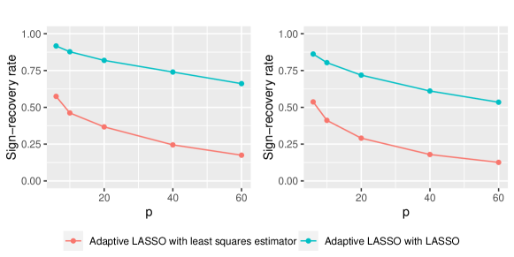
  Figure 1: left chart shows the sign-recovery rate for $\mathcal{U}[-1,1]$ distributed regressors, right one for $\mathcal{U}\{-1,0,1\}$ distributed regressors. The sample size is always $n=5.000$.

  

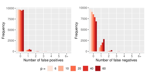
  Figure 2: frequency of false positives and false negatives for adaptive LASSO with LASSO as inital estimator, $\mathcal{U}[-1,1]$ distributed regressors and sample size $n=5.000$.

  

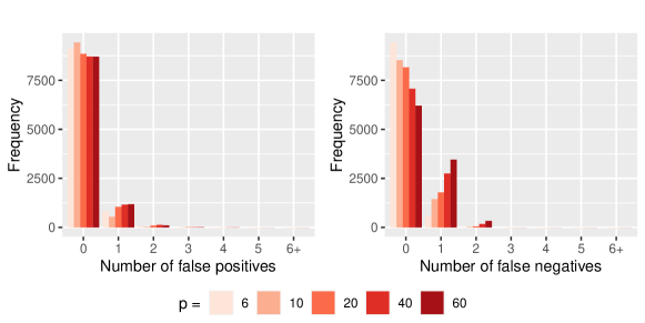
  Figure 3: frequency of false positives and false negatives for adaptive LASSO with LASSO as inital estimator, $\mathcal{U}\{-1,0,1\}$ distributed regressors and sample size $n=5.000$.

• Sample size $\boldsymbol{n=10.000}$.
  In this setting the sign-recovery rate is in all scenarios much higher than in the first one with $n=5000$. In the bar charts of the false positives and false negatives there are no unexpected results to detect.

  

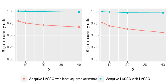
  Figure 4: left chart shows the sign-recovery rate for $\mathcal{U}[-1,1]$ distributed regressors, right one for $\mathcal{U}\{-1,0,1\}$ distributed regressors. The sample size is always $n=10.000$.

  

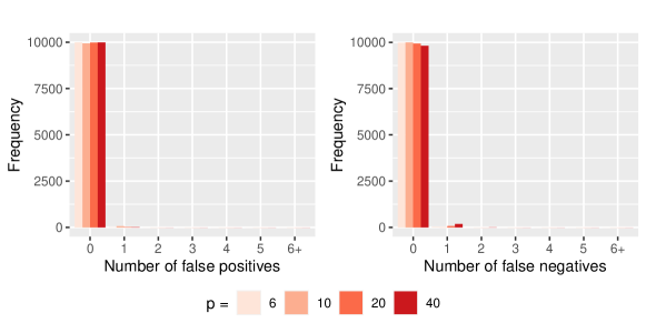
  Figure 5: frequency of false positives and false negatives for adaptive LASSO with LASSO as inital estimator, $\mathcal{U}[-1,1]$ distributed regressors and sample size $n=10.000$.

  

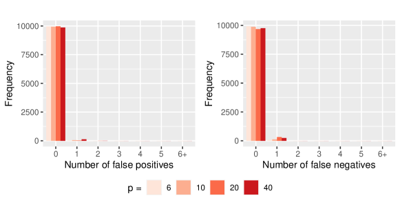
  Figure 6: frequency of false positives and false negatives for adaptive LASSO with LASSO as inital estimator, $\mathcal{U}\{-1,0,1\}$ distributed regressors and sample size $n=10.000$.

For comparison, we also present a figure for the sign-recovery rate for the mean in Figure 7. Here, even with the simple least squares estimator as initial estimator, the sign-recovery rate is already very high for sample size $n=5000$.

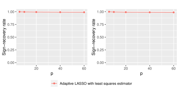
Figure 7: left chart shows the sign-recovery rate for $\mathcal{U}[-1,1]$ distributed regressors, right one for $\mathcal{U}\{-1,0,1\}$ distributed regressors. The sample size is always $n=5.000$.

5 Proofs of the main results

5.1 Proofs for Section 2

Proofs of Propositions 1 and 2

Proof of Proposition 1.

Set $u=\sqrt{{\operatorname{\mathbb{V}\mathrm{ar}}}(B_{1})}$. From $s_{2}^{2}=s_{1}^{2}+u^{2}+2\,\rho\,s_{1}\,u$ and $|\rho|\leq 1$ we obtain the inequalities

$$(u-s_{1})^{2}\leq s_{2}^{2}\leq(u+s_{1})^{2}.$$

By equating $s_{2}^{2}=(u+s_{1})^{2}$ we obtain the solutions $\pm s_{2}-s_{1}$ for $u$, which yields $u\geq s_{2}-s_{1}$ if $s_{2}>s_{1}.$ If $s_{2}\leq s_{1}$ we obviously have only the bound $u\geq 0$. Equating $s_{2}^{2}=(u-s_{1})^{2}$ gives the solutions $\pm s_{2}+s_{1}$ for $u$, which yields the bounds

$$u\in\big{[}|s_{1}-s_{2}|,s_{1}+s_{2}\big{]}$$

for the standard deviation $u=\sqrt{{\operatorname{\mathbb{V}\mathrm{ar}}}(B_{1})}$. Solving the equation at the beginning for the correlation gives $\rho=(s_{2}^{2}-s_{1}^{2}-u^{2})/(2\,s_{1}u)$, which ranges over the whole interval $[-1,1]$ if $s_{2}>s_{1}$. If $s_{1}\geq s_{2}$, the correlation must be negative, and maximizing the above expression for $\rho$ over $u$ yields $u=\sqrt{s_{1}^{2}-s_{2}^{2}}$, and finally the upper bound in (4). ∎

Proof of Proposition 2.

It is enough to show that all mixed moments of order $n$ are identified from $n+1$ support points, the claim then follows by induction. By model (3) we obtain

$${\mathbb{E}}\big{[}Y^{n}\,\big{|}\,W_{1}=w\big{]}={\mathbb{E}}\big{[}(B_{0}+w\,B_{1})^{n}\big{]}=\sum_{k=0}^{n}\binom{n}{k}\,w^{k}\,{\mathbb{E}}\big{[}B_{0}^{n-k}\,B_{1}^{k}\big{]}.$$

If $W$ has distinct support points $w_{1},\dotsc,w_{n+1}$, we obtain a linear system for the moments ${\mathbb{E}}\big{[}B_{0}^{n-k}\,B_{1}^{k}\big{]}$, $k=0,\dotsc,n$. Its design matrix satisfies

$$\det\Bigg{(}\binom{n}{k-1}w_{j}^{k-1}\Bigg{)}_{j,k\in\{1,\dotsc,n+1\}} =\prod_{l=0}^{n}\binom{n}{l}\ \det\Big{(}w_{j}^{k-1}\Big{)}_{j,k\in\{1,\dotsc,n+1\}}$$

$$=\prod_{l=0}^{n}\binom{n}{l}\ \prod_{1\leq j<k\leq n+1}(w_{k}-w_{j})\not=0\,,$$

so that the solution is unique. In the last equation we used the determinant of the Vandermonde matrix. ∎

Proof of Theorem 3

The proof needs some preparations. Recall that points ${\mathbf{w_{1}}},\dotsc,{\mathbf{w_{d}}}\in{\mathbb{R}}^{d-1}$ are said to be in general position if $\sum_{k=1}^{d}\alpha_{k}{\mathbf{w_{k}}}={\mathbf{0}}_{d-1}$ for $\alpha_{k}\in{\mathbb{R}}$, $\sum_{k=1}^{d}\alpha_{k}=0$, implies that $\alpha_{1}=\dotsc=\alpha_{d}=0$. The following result is well-known.

Lemma 1.

Points ${\mathbf{w_{1}}},\dotsc,{\mathbf{w_{d}}}\in{\mathbb{R}}^{d-1}$ are in general position if and only if one of the following conditions holds.

1. ${\mathbf{w_{2}}}-{\mathbf{w_{1}}},\dotsc,{\mathbf{w_{d}}}-{\mathbf{w_{1}}}$ are linearly independent.

2. For each $j\in\{1,\dotsc,d\}$ the point ${\mathbf{w_{j}}}$ is not contained in $\big{\{}\sum_{k=1,k\not=j}^{d}\alpha_{k}{\mathbf{w_{k}}}\mid\sum_{k=1,k\not=j}^{d}\alpha_{k}=1\big{\}}$, the hyperplane generated by ${\mathbf{w_{k}}},k\not=j$.

Lemma 2.

If the support of ${\mathbf{W}}$ contains $p$ points ${\mathbf{w_{1}}},\dotsc,{\mathbf{w_{p}}}\in{\mathbb{R}}^{p-1}$ in general position, then the means $\mu^{*}={\mathbb{E}}[{\mathbf{A}}]$ are identified.

Proof of Lemma 2.

The design matrix of the linear system ${\mathbb{E}}[Y\,|\,{\mathbf{W}}={\mathbf{w_{j}}}]={\mathbb{E}}[B_{0}]+{\mathbf{w_{j}^{\top}}}{\mathbb{E}}[{\mathbf{B}}]$, $j=1,\dotsc,p$, has the same rank as the matrix

$$\begin{bmatrix}1&{\mathbf{w_{1}^{\top}}}\\ 0&{\mathbf{w_{2}^{\top}}}-{\mathbf{w_{1}^{\top}}}\\ \vdots&\vdots\\ 0&{\mathbf{w_{p}^{\top}}}-{\mathbf{w_{1}^{\top}}}\end{bmatrix}\,,$$

which is invertible by Lemma 1. ∎

Proof of Theorem 3.

Suppose that $S$ is of full rank. Since $S$ contains the matrix

$$\begin{bmatrix}1&2{\mathbf{w_{1}^{\top}}}\\ \vdots&\vdots\\ 1&2{\mathbf{w_{p(p+1)/2}^{\top}}}\end{bmatrix}\quad\in{\mathbb{R}}^{\frac{p(p+1)}{2}\times p}$$

as a submatrix, in order for $S$ to have full rank, it is necessary that this submatrix has rank $p$. This implies that there are $p$ points among the support points ${\mathbf{w_{1}}},\dotsc,{\mathbf{w_{p(p+1)/2}}}$ in general position, thus identifying the means by Lemma 2. Then, the linear system which determines ${\operatorname{\mathbb{V}\mathrm{ar}}}(Y\,|\,{\mathbf{W}}={\mathbf{w_{j}}})$ in terms of the entries of $\Sigma^{*}$ has full-rank design matrix $S$, see (2.1), thus identifying $\Sigma^{*}$ from the conditional variances.

Conversely, let $m=p(p+1)/2$. Suppose that the condition is not satisfied, then all support points ${\mathbf{w}}$ of ${\mathbf{W}}$ are such that the vectors ${\operatorname{v}}\big{(}(1,{\mathbf{w^{\top}}})^{\top}\big{)}$ are contained in an $(m-1)$-dimensional linear subspace $V$ of ${\mathbb{R}}^{m}$. The $p\times p$-dimensional positive semi-definite matrices form a convex cone with interior consisting of positive definite matrices in the space of all $p\times p$-dimensional symmetric matrices. The image under the map ${\operatorname{vec}}$ is thus a convex cone $\mathcal{C}\subset{\mathbb{R}}^{m}$ with non-empty interior in ${\mathbb{R}}^{m}$.

Let ${\mathbf{z}}$ be a unit vector orthogonal to $V$, and let $Z$ be the $p\times p$-dimensional symmetric matrix for which ${\operatorname{vec}}(Z)={\mathbf{z}}$. Since the positive definite matrices are open in the space of all $p\times p$-dimensional symmetric matrices, given a positive definite matrix $\Sigma^{*}$, for small $\epsilon>0$ the matrix $\Sigma_{1}=\Sigma^{*}+\epsilon\,Z$ will still be positive definite, and hence a covariance matrix. Moreover, it is ${\operatorname{vec}}(\Sigma_{1})={\operatorname{vec}}(\Sigma^{*})+\epsilon\,{\operatorname{vec}}(Z)={\operatorname{vec}}(\Sigma^{*})+\epsilon\,{\mathbf{z}}$ and $(1,{\mathbf{w^{\top}}})\,Z\,(1,{\mathbf{w^{\top}}})^{\top}={\operatorname{v}}\big{(}(1,{\mathbf{w^{\top}}})^{\top}\big{)}^{\top}\,{\mathbf{z}}=0$ for ${\mathbf{w}}$ in the support of ${\mathbf{W}}$ by construction. Hence the conditional variances $(1,{\mathbf{w^{\top}}})\,\Sigma^{*}\,(1,{\mathbf{w^{\top}}})^{\top}$ and $(1,{\mathbf{w^{\top}}})\,\Sigma_{1}\,(1,{\mathbf{w^{\top}}})^{\top}$ will be the same over the support of ${\mathbf{W}}$. Thus, for normally distributed ${\mathbf{A}}\sim\mathcal{N}_{p}({\mathbf{0}}_{p},\Sigma^{*})$ or ${\mathbf{A}}\sim\mathcal{N}_{p}({\mathbf{0}}_{p},\Sigma_{1})$, the conditional normal distributions of $Y\,|\,{\mathbf{W}}={\mathbf{w}}$ will coincide, showing nonidentifiability. ∎

Proof of Theorem 4

For the proof of the theorem, we require the following lemma.

Lemma 3.

Suppose that the support of ${\mathbf{W}}$ in (1) contains points satisfying the following properties.

1. The $p$ points ${\mathbf{w_{1}}},\dotsc,{\mathbf{w_{p}}}\in{\mathbb{R}}^{p-1}$ are in general position.

2. For each $j\in\{1,\dotsc,p\}$ there exist points ${\mathbf{w_{j,1}}},\dotsc,{\mathbf{w_{j,p-1}}}\in{\mathbb{R}}^{p-1}$, possibly equal to those in 1., such that

   • ${\mathbf{w_{j}}},{\mathbf{w_{j,1}}},\dotsc,{\mathbf{w_{j,p-1}}}$ are in general position,

   • for each $j\in\{1,\dotsc,p\}$, $k\in\{1,\dotsc,p-1\}$ there is a ${\mathbf{z_{j,k}}}\in{\mathbb{R}}^{p-1}$ for which ${\mathbf{w_{j}}},{\mathbf{w_{j,k}}},{\mathbf{z_{j,k}}}$ are all distinct but generate only a one-dimensional affine space, i.e. are all contained in a line.

Then the design matrix $S$ in (9) formed from all the points ${\mathbf{w_{j}}},{\mathbf{w_{j,k}}},{\mathbf{z_{j,k}}}$ has full rank $p(p+1)/2$ and hence, the mean vector $\mu^{*}$ and the covariance matrix $\Sigma^{*}$ of the random coefficients ${\mathbf{A}}$ are identified.

The minimal number of support points required in this lemma is $p+p(p-1)/2=p(p+1)/2$, which corresponds to the number of free parameters in $\Sigma^{*}$. For the proof of Lemma 3 we first need the following two preliminary lemmas.

Lemma 4.

Suppose that $\Sigma$ is a $p\times p$-dimensional symmetric matrix and ${\mathbf{v_{1}}},\dotsc,{\mathbf{v_{p}}}\in{\mathbb{R}}^{p}$ is a known basis of ${\mathbb{R}}^{p}$. If ${\mathbf{v}}\in{\mathbb{R}}^{p}$ and ${\mathbf{v^{\top}}}\Sigma\,{\mathbf{v_{j}}}$, $1\leq j\leq p$, is identified, then ${\mathbf{v^{\top}}}\Sigma\,{\mathbf{u}}$ is identified for any vector ${\mathbf{u}}\in{\mathbb{R}}^{p}$. In particular, $\Sigma$ is identified from the values ${\mathbf{v_{j}^{\top}}}\Sigma\,{\mathbf{v_{k}}}$, $1\leq j\leq k\leq p$.

Proof of Lemma 4.

Given ${\mathbf{u}}\in{\mathbb{R}}^{p}$ we may write ${\mathbf{u}}=\sum_{j=1}^{p}\lambda_{j}{\mathbf{v_{j}}}$ with $\lambda_{1},\dotsc,\lambda_{p}\in{\mathbb{R}}$. Then

$${\mathbf{v^{\top}}}\Sigma\,{\mathbf{u}}=\sum_{j=1}^{p}\lambda_{j}{\mathbf{v^{\top}}}\Sigma\,{\mathbf{v_{j}}}\,,$$

showing the first claim. For the second, let $e_{k}=(0,\dotsc,0,1,0,\dotsc,0)^{\top}$ denote the $k^{\text{th}}$ unit vector in ${\mathbb{R}}^{p}$. By assumption, one may write $e_{k}=\sum_{j=1}^{p}\lambda_{k,j}{\mathbf{v_{j}}}$, where $\lambda_{k,j}\in{\mathbb{R}}$ and $1\leq k\leq p$. Then

$$\Sigma_{kl}=e_{k}^{\top}\Sigma\,e_{l}=\sum_{j_{1},j_{2}=1}^{p}\lambda_{k,j_{1}}\lambda_{l,j_{2}}{\mathbf{v_{j_{1}}^{\top}}}\Sigma\,{\mathbf{v_{j_{2}}}}\,.$$

The result follows from the assumptions and the symmetry of $\Sigma$. ∎

Lemma 5.

Let ${\mathbf{v_{1}}},{\mathbf{v_{2}}},{\mathbf{v_{3}}}\in{\mathbb{R}}^{p}$ be such that each pair is linearly independent, but all three are linearly dependent, so that ${\mathbf{v_{3}}}=\lambda_{1}{\mathbf{v_{1}}}+\lambda_{2}{\mathbf{v_{2}}}$, where $\lambda_{1},\lambda_{2}\not=0$. Then for a $p\times p$-dimensional symmetric matrix $\Sigma$ it holds that

$${\mathbf{v_{1}^{\top}}}\Sigma\,{\mathbf{v_{2}}}=\frac{1}{2\,\lambda_{1}\lambda_{2}}\Big{(}{\mathbf{v_{3}^{\top}}}\Sigma\,{\mathbf{v_{3}}}-\lambda_{1}^{2}\,{\mathbf{v_{1}^{\top}}}\Sigma\,{\mathbf{v_{1}}}-\lambda_{2}^{2}\,{\mathbf{v_{2}^{\top}}}\Sigma\,{\mathbf{v_{2}}}\Big{)}\,.$$

Proof of Lemma 5.

Plug in the expression for ${\mathbf{v_{3}}}$ and compute the right side of the equation. ∎

Proof of Lemma 3.

By Lemma 2 and the first assumption the means $\mu^{*}$ are identified. Hence we obtain the equations (6) or equivalently (2.1) with ${\mathbf{w}}$ ranging over the support points mentioned in the statement of the lemma. To show that the design matrix $S$ in (9) has full rank $p(p+1)/2$, it suffices to show that from these equations one can uniquely solve for $\sigma^{*}$. To this end, from the second assumption, for $j\in\{1,\dotsc,p\}$ and $k\in\{1,\dotsc,p-1\}$, letting ${\mathbf{v_{1}}}=(1,{\mathbf{w_{j}^{\top}}})^{\top}$, ${\mathbf{v_{2}}}=(1,{\mathbf{w_{j,k}^{\top}}})^{\top}$ and ${\mathbf{v_{3}}}=(1,{\mathbf{z_{j,k}^{\top}}})^{\top}$ in Lemma 5 we identify $(1,{\mathbf{w_{j}^{\top}}})\,\Sigma^{*}\,(1,{\mathbf{w_{j,k}^{\top}}})^{\top}$. Since $(1,{\mathbf{w_{j}^{\top}}})\,\Sigma^{*}\,(1,{\mathbf{w_{j}^{\top}}})^{\top}$ are also identified, from the first part in Lemma 4 we identify $(1,{\mathbf{w_{j}^{\top}}})\,\Sigma^{*}\,(1,{\mathbf{w_{l}^{\top}}})^{\top}$, $j,l\in\{1,\dotsc,p\}$. Hence from the second part of that lemma and the first assumption $\Sigma^{*}$ itself is identified. ∎

Proof of Theorem 4.

For the sufficiency, suppose that the support of $W_{j}$ contains $\{w_{j,k},\ k=1,2,3\}$, $j=1,\dotsc,p-1$. We apply Lemma 3 with

• ${\mathbf{w_{j}}}=(w_{1,1},\dotsc,w_{j-1,1},w_{j,2},w_{j+1,1},\dotsc,w_{p-1,1})^{\top}$, $j=1,\dotsc,p-1$, and ${\mathbf{w_{p}}}=(w_{1,1},\dotsc,w_{p-1,1})^{\top}$,

• for $j\in\{1,\dotsc,p-1\}$, let ${\mathbf{w_{j,k}}}$, $k\in\{1,\dotsc,p-1\}$, $k\not=j$, enumerate the points having $k^{\text{th}}$ coordinate $w_{k,2}$ and $j^{\text{th}}$ coordinate $w_{j,2}$, otherwise coordinates $w_{i,1}$, the corresponding ${\mathbf{z_{j,k}}}$ having $k^{\text{th}}$ coordinate $w_{k,3}$, $j^{\text{th}}$ coordinate $w_{j,2}$, otherwise coordinates $w_{i,1}$. Furthermore, let ${\mathbf{w_{j,j}}}={\mathbf{w_{p}}}$ and let ${\mathbf{z_{j,j}}}$ have $j^{\text{th}}$ coordinate $w_{j,3}$, otherwise $w_{i,1}$,

• let ${\mathbf{w_{p,k}}}={\mathbf{w_{k}}}$, $k\in\{1,\dotsc,p-1\}$, and ${\mathbf{z_{p,k}}}=(w_{1,1},\dotsc,w_{k-1,1},w_{k,3},w_{k+1,1},\dotsc,w_{p-1,1})^{\top}$.

The requirements of the lemma are then easily checked by applying Lemma 1, 1. The necessity of at least three support points in each coordinate, if $\Sigma^{*}$ has full rank, is clear from Example 1. ∎

5.1.1 Proofs for Section 2.2

Proof of Proposition 5.

The claims in 1. are clear. For 2., in both cases, from ${\operatorname{\mathbb{V}\mathrm{ar}}}(B_{0})={\operatorname{\mathbb{V}\mathrm{ar}}}(B_{0}+B_{1})$ we get that

$${\operatorname{\mathbb{V}\mathrm{ar}}}(B_{1})=-2\,{\operatorname{\mathbb{C}\mathrm{ov}}}(B_{0},B_{1})\,.$$

Since the covariance matrix ${\operatorname{\mathbb{C}\mathrm{ov}}}\big{(}(B_{0},B_{1},{\mathbf{B_{2}^{\top}}})^{\top}\big{)}$ is positive semi-definite, setting $s={\operatorname{\mathbb{V}\mathrm{ar}}}(B_{1})$, we hence require

$$s\,(z^{2}-zv_{1})+{\mathbf{v^{\top}}}{\operatorname{\mathbb{C}\mathrm{ov}}}\big{(}(B_{0},{\mathbf{B_{2}^{\top}}})^{\top}\big{)}\,{\mathbf{v}}\geq 0$$ (25)

for any $z\in{\mathbb{R}}$, ${\mathbf{v}}=(v_{1},\dotsc,v_{p-1})^{\top}\in{\mathbb{R}}^{p-1}$.

1. Choose ${\mathbf{v}}\in{\mathbb{R}}^{p-1}$ in the kernel of ${\operatorname{\mathbb{C}\mathrm{ov}}}\big{(}(B_{0},{\mathbf{B_{2}^{\top}}})^{\top}\big{)}$ for which $v_{1}>0$. If we assume $s>0$, then for $0<z<v_{1}$ the form in (25) would be negative. Hence $s=0$ in this case.

2. If ${\operatorname{\mathbb{C}\mathrm{ov}}}\big{(}(B_{0},{\mathbf{B_{2}^{\top}}})^{\top}\big{)}$ has full rank, then for the minimal eigenvalue $\lambda_{\min}>0$ of ${\operatorname{\mathbb{C}\mathrm{ov}}}\big{(}(B_{0},{\mathbf{B_{2}^{\top}}})^{\top}\big{)}$ we have that

   $${\mathbf{v^{\top}}}{\operatorname{\mathbb{C}\mathrm{ov}}}\big{(}(B_{0},{\mathbf{B_{2}^{\top}}})^{\top}\big{)}\,{\mathbf{v}}\geq\lambda_{\min}\,{\left\lVert v\right\rVert_{2}^{2}}\,.$$

   Therefore, the form in (25) is positive definite for $0\leq s\leq 4\,\lambda_{\min}$.

∎

Proof of Theorem 6.

By (13), the symmetric multilinear form

$$u({\mathbf{v}}_{1},\ldots,{\mathbf{v}}_{k})={\mathbb{E}}\big{[}({\mathbf{A}}^{\top}{\mathbf{v}}_{1})\cdot\ldots\cdot({\mathbf{A}}^{\top}{\mathbf{v}}_{k})\big{]},\qquad{\mathbf{v}}_{j}\in{\mathbb{R}}^{p},\quad j=1,\ldots,k,$$

is identified over the diagonal

$$\tilde{u}({\mathbf{v}})=u({\mathbf{v}},\ldots,{\mathbf{v}})$$

for ${\mathbf{v}}^{\top}=(1,{\mathbf{w}}^{\top})$ with ${\mathbf{w}}$ in the support of ${\mathbf{W}}$.

We shall show that the symmetric multilinear form $u$ is identified. Then, inserting unit vectors $(0,\ldots,0,1,0,\ldots,0)$ yields the $k^{\text{th}}$ -order mixed moments.

By multilinearity, it sufficies to show that $u$ is identified over a basis of ${\mathbb{R}}^{p}$, that is, there exists a basis ${\mathbf{v_{1}}},\ldots,{\mathbf{v_{p}}}$ of ${\mathbb{R}}^{p}$ such that $u({\mathbf{v}}_{i_{1}},\ldots,{\mathbf{v}}_{i_{k}})$ is identified for all choices $i_{j}\in\{1,\ldots,p\}$. To this end, we use the polarization formula for symmetric multilinear forms (Thomas, 2014, formula (7) ), which we write as

$$u({\mathbf{v}}_{1},\ldots,{\mathbf{v}}_{k})=\frac{1}{k!}\,\sum_{j=1}^{k}\,(-1)^{k-j}\,\sum_{\{i_{1},\ldots i_{j}\}\subseteq\{1,\ldots,k\}}\,j^{k}\,\tilde{u}\big{(}({\mathbf{v}}_{i_{1}}+\ldots+{\mathbf{v}}_{i_{j}})/j\big{)}.$$ (26)

Now for ${\mathbf{w}}_{1},\ldots,{\mathbf{w}}_{p}$ as in the assumption of the theorem, the vectors $(1,{\mathbf{w}}_{i}^{\top})$, $i=1,\ldots,p$ are linearly independent by the proof of Lemma 2, and for $j\in\{1,\ldots,k\}$ and $i_{1},\ldots,i_{j}\in\{1,\ldots,p\}$ we have

$$\big{(}(1,{\mathbf{w}}_{i_{1}}^{\top})+\ldots+(1,{\mathbf{w}}_{i_{j}}^{\top})\big{)}/j=\big{(}1,({\mathbf{w}}_{i_{1}}+\ldots+{\mathbf{w}}_{i_{j}})^{\top}/j\big{)}$$

with $({\mathbf{w}}_{i_{1}}+\ldots+{\mathbf{w}}_{i_{j}})^{\top}/j$ in the support of ${\mathbf{W}}$. Hence the terms on the right of (26) are identified for $k$ (not necessarily distinct) vectors $(1,{\mathbf{w}}_{i}^{\top})$, thus also the form $u$. ∎

5.2 Proofs for Section 3.2

Proof of Theorem 10

Consider the following decomposition of the error term (17):

$${\varepsilon_{n}^{\sigma}}=\delta_{n}+\zeta_{n}+\xi_{n}$$ (27)

with

$$\delta_{n} \mathrel{\vbox{\hbox{\scriptsize.}\hbox{\scriptsize.}}}=\Big{(}{\operatorname{v}}\big{(}{\mathbf{X_{1}}}\big{)}^{\top}{\operatorname{vec}}\big{(}D_{1}-\Sigma^{*}\big{)},\dotsc,{\operatorname{v}}\big{(}{\mathbf{X_{n}}}\big{)}^{\top}{\operatorname{vec}}\big{(}D_{n}-\Sigma^{*}\big{)}\Big{)}^{\top}\,,$$ (28)

$$\zeta_{n} \mathrel{\vbox{\hbox{\scriptsize.}\hbox{\scriptsize.}}}=\Big{(}{\operatorname{v}}\big{(}{\mathbf{X_{1}}}\big{)}^{\top}{\operatorname{vec}}\big{(}E_{n}\big{)},\dotsc,{\operatorname{v}}\big{(}{\mathbf{X_{n}}}\big{)}^{\top}{\operatorname{vec}}\big{(}E_{n}\big{)}\Big{)}^{\top}\,,$$

$$\xi_{n} \mathrel{\vbox{\hbox{\scriptsize.}\hbox{\scriptsize.}}}=\Big{(}{\operatorname{v}}\big{(}{\mathbf{X_{1}}}\big{)}^{\top}{\operatorname{vec}}\big{(}F_{n,1}\big{)},\dotsc,{\operatorname{v}}\big{(}{\mathbf{X_{n}}}\big{)}^{\top}{\operatorname{vec}}\big{(}F_{n,n}\big{)}\Big{)}^{\top}\,.$$

The matrices $D_{1},\dotsc,D_{n},E_{n},F_{n,1},\dotsc,F_{n,n}$ are defined in (15) and (16).

For the proof of Theorem 10 we need the following auxiliary lemmas.

Lemma 6.

Set $Z_{n}^{\sigma,1}=\frac{1}{n}\,\big{(}{{\mathbb{X}}_{n}^{\sigma}}\big{)}^{\top}\delta_{n}$, then $\big{\|}Z_{n}^{\sigma,1}\big{\|}_{2}={\operatorname{\mathcal{O}_{\mathbb{P}}}\left(p/\sqrt{n}\right)}$.

Proof of Lemma 6.

It is

$${\mathbb{E}}\Big{[}{\left\lVert Z_{n}^{\sigma,1}\right\rVert_{2}^{2}}\Big{]} =\frac{1}{n^{2}}\,{\mathbb{E}}\Big{[}\delta_{n}^{\top}{{\mathbb{X}}_{n}^{\sigma}}\,({{\mathbb{X}}_{n}^{\sigma}})^{\top}\delta_{n}\Big{]}=\frac{1}{n^{2}}\,{\mathbb{E}}\Big{[}{\operatorname{trace}}\big{(}({{\mathbb{X}}_{n}^{\sigma}})^{\top}\delta_{n}\,\delta_{n}^{\top}{{\mathbb{X}}_{n}^{\sigma}}\big{)}\Big{]}$$

$$=\frac{1}{n^{2}}\,{\mathbb{E}}\Big{[}{\operatorname{trace}}\big{(}({{\mathbb{X}}_{n}^{\sigma}})^{\top}{\mathbb{E}}\big{[}\delta_{n}\,\delta_{n}^{\top}\,\big{|}\,{{\mathbb{X}}_{n}^{\sigma}}\big{]}\,{{\mathbb{X}}_{n}^{\sigma}}\big{)}\Big{]}=\frac{1}{n}\,{\operatorname{trace}}\Bigg{(}{\mathbb{E}}\bigg{[}\frac{1}{n}\,({{\mathbb{X}}_{n}^{\sigma}})^{\top}\Omega_{n}^{\sigma}\,{{\mathbb{X}}_{n}^{\sigma}}\bigg{]}\Bigg{)}\,,$$

where $\Omega_{n}^{\sigma}={\operatorname{\mathbb{C}\mathrm{ov}}}\big{(}\delta_{n}\,\big{|}\,{{\mathbb{X}}_{n}^{\sigma}}\big{)}$ is given in Lemma 10. It is obvious that

$${\mathbb{E}}\bigg{[}\frac{1}{n}\,({{\mathbb{X}}_{n}^{\sigma}})^{\top}\Omega_{n}^{\sigma}\,{{\mathbb{X}}_{n}^{\sigma}}\bigg{]}=\mathrm{B}^{\sigma}\,,$$

and hence we obtain by Assumption (A7) the estimate

$${\mathbb{E}}\Big{[}{\left\lVert Z_{n}^{\sigma,1}\right\rVert_{2}^{2}}\Big{]} =\frac{{\operatorname{trace}}\big{(}\mathrm{B}^{\sigma}\big{)}}{n}\leq\frac{\lambda_{\max}\big{(}\mathrm{B}^{\sigma}\big{)}\,p(p+1)}{2n}\leq\frac{{c_{\,\mathrm{B}^{\sigma},\mathrm{u}}}\,p(p+1)}{2n}\,.$$

Markov’s inequality implies the assertion. ∎

Lemma 7.

Set $Z_{n}^{\sigma,2}=\frac{1}{n}\,\big{(}{{\mathbb{X}}_{n}^{\sigma}}\big{)}^{\top}\zeta_{n}$, then $\big{\|}Z_{n}^{\sigma,2}\big{\|}_{2}={\operatorname{\mathcal{O}_{\mathbb{P}}}\left(p/n\right)}$.

Proof of Lemma 7.

It is

$${\left\lVert Z_{n}^{\sigma,2}\right\rVert_{2}} ={\left\lVert\frac{1}{n}\,\sum_{i=1}^{n}\big{(}e_{i}^{\top}\zeta_{n}\big{)}{\operatorname{v}}\big{(}{\mathbf{X_{i}}}\big{)}\right\rVert_{2}}={\left\lVert\frac{1}{n}\,\sum_{i=1}^{n}\Big{(}{\operatorname{v}}\big{(}{\mathbf{X_{i}}}\big{)}^{\top}{\operatorname{vec}}\big{(}E_{n}\big{)}\Big{)}{\operatorname{v}}\big{(}{\mathbf{X_{i}}}\big{)}\right\rVert_{2}}$$

$$\leq{\left\lVert\frac{1}{n}\,\sum_{i=1}^{n}{\operatorname{v}}\big{(}{\mathbf{X_{i}}}\big{)}\,{\operatorname{v}}\big{(}{\mathbf{X_{i}}}\big{)}^{\top}\right\rVert_{\mathrm{M},2}}\,{\left\lVert{\operatorname{vec}}\big{(}E_{n}\big{)}\right\rVert_{2}}\,.$$

We multiply each entry of $E_{n}$, which is not on the diagonal, with $\sqrt{2}$ and denote the resulting matrix by $\widetilde{E}_{n}$. Then it is clear that ${\left\lVert{\operatorname{vec}}\big{(}E_{n}\big{)}\right\rVert_{2}}\leq\big{\|}{\operatorname{vec}}\big{(}\widetilde{E}_{n}\big{)}\big{\|}_{2}$ and $\big{\|}{\operatorname{vec}}\big{(}\widetilde{E}_{n}\big{)}\big{\|}_{2}={\left\lVert E_{n}\right\rVert_{\mathrm{F}}}$. Moreover, recall that $E_{n}=\big{(}\mu^{*}-\widehat{\mu}_{n}\big{)}\big{(}\mu^{*}-\widehat{\mu}_{n}\big{)}^{\top}$ is a rank-one matrix and hence ${\left\lVert E_{n}\right\rVert_{\mathrm{F}}}\leq{\left\lVert\widehat{\mu}_{n}-\mu^{*}\right\rVert_{2}^{2}}$. Hence we obtain

$$\frac{n}{p}\,{\left\lVert Z_{n}^{\sigma,2}\right\rVert_{2}}\leq{\left\lVert\frac{1}{n}\,\big{(}{{\mathbb{X}}_{n}^{\sigma}}\big{)}^{\top}{{\mathbb{X}}_{n}^{\sigma}}\right\rVert_{\mathrm{M},2}}\,\frac{n}{p}\,{\left\lVert\widehat{\mu}_{n}-\mu^{*}\right\rVert_{2}^{2}}={\operatorname{\mathcal{O}_{\mathbb{P}}}\left(1\right)}\,{\operatorname{\mathcal{O}_{\mathbb{P}}}\left(1\right)}={\operatorname{\mathcal{O}_{\mathbb{P}}}\left(1\right)}$$

since $\sqrt{n/p}\,{\left\lVert\widehat{\mu}_{n}-\mu^{*}\right\rVert_{2}}={\operatorname{\mathcal{O}_{\mathbb{P}}}\left(1\right)}$. ∎

Lemma 8.

Set $Z_{n}^{\sigma,3}=\frac{1}{n}\,\big{(}{{\mathbb{X}}_{n}^{\sigma}}\big{)}^{\top}\xi_{n}$, then $\big{\|}Z_{n}^{\sigma,3}\big{\|}_{2}={\operatorname{\mathcal{O}_{\mathbb{P}}}\left(p^{3/2}/n^{5/8}+p^{2}/n^{3/4}\right)}$. In particular, we obtain by Assumption (A8) the convergence $\sqrt{n}/p\,\big{\|}Z_{n}^{\sigma,3}\big{\|}_{2}={\operatorname{\mathcal{O}_{\mathbb{P}}}\left(p^{1/2}/n^{1/8}+p/n^{1/4}\right)}={\operatorname{o_{\mathbb{P}}}\left(1\right)}$.

Proof of Lemma 8.

It is

$${\left\lVert Z_{n}^{\sigma,3}\right\rVert_{2}} ={\left\lVert\frac{1}{n}\,\sum_{i=1}^{n}\big{(}e_{i}^{\top}\xi_{n}\big{)}{\operatorname{v}}\big{(}{\mathbf{X_{i}}}\big{)}\right\rVert_{2}}=2\,{\left\lVert\frac{1}{n}\,\sum_{i=1}^{n}\Big{(}{\mathbf{X_{i}^{\top}}}\big{(}{\mathbf{A_{i}}}-\mu^{*}\big{)}\,{\mathbf{X_{i}^{\top}}}\big{(}\mu^{*}-\widehat{\mu}_{n}\big{)}\Big{)}{\operatorname{v}}\big{(}{\mathbf{X_{i}}}\big{)}\right\rVert_{2}}$$

$$\leq 2\,{\left\lVert\frac{1}{n}\,\sum_{i=1}^{n}\Big{(}{\mathbf{X_{i}^{\top}}}\big{(}{\mathbf{A_{i}}}-\mu^{*}\big{)}\Big{)}{\operatorname{v}}\big{(}{\mathbf{X_{i}}}\big{)}\,{\mathbf{X_{i}^{\top}}}\right\rVert_{\mathrm{M},2}}\,{\left\lVert\mu^{*}-\widehat{\mu}_{n}\right\rVert_{2}}\,,$$ (29)

and we have again $\sqrt{n/p}\,{\left\lVert\widehat{\mu}_{n}-\mu^{*}\right\rVert_{2}}={\operatorname{\mathcal{O}_{\mathbb{P}}}\left(1\right)}$. Moreover, let

$$\mathcal{T}_{n}(\tau_{n})=\bigcap_{i=1}^{n}\Big{\{}{\left\lVert{\mathbf{A_{i}}}-\mu^{*}\right\rVert_{2}}\leq\tau_{n}\Big{\}}$$

with $\tau_{n}>0$, then we obtain

$$\bigg{\|}\frac{1}{n}\,\sum_{i=1}^{n}\Big{(}{\mathbf{X_{i}^{\top}}}\big{(}{\mathbf{A_{i}}}-\mu^{*}\big{)}\Big{)}{\operatorname{v}}\big{(}{\mathbf{X_{i}}}\big{)}\,{\mathbf{X_{i}^{\top}}}\bigg{\|}_{\mathrm{M},2}$$

$$\leq\bigg{\|}\frac{1}{n}\,\sum_{i=1}^{n}\Big{(}{\mathbf{X_{i}^{\top}}}\big{(}{\mathbf{A_{i}}}-\mu^{*}\big{)}\Big{)}{\operatorname{v}}\big{(}{\mathbf{X_{i}}}\big{)}\,{\mathbf{X_{i}^{\top}}}\,\mathbbm{1}_{\mathcal{T}_{n}(\tau_{n})}\bigg{\|}_{\mathrm{M},2}+\bigg{\|}\frac{1}{n}\,\sum_{i=1}^{n}\Big{(}{\mathbf{X_{i}^{\top}}}\big{(}{\mathbf{A_{i}}}-\mu^{*}\big{)}\Big{)}{\operatorname{v}}\big{(}{\mathbf{X_{i}}}\big{)}\,{\mathbf{X_{i}^{\top}}}\,\mathbbm{1}_{\mathcal{T}_{n}^{c}(\tau_{n})}\bigg{\|}_{\mathrm{M},2}$$

$$\leq\Bigg{\|}\frac{1}{n}\,\sum_{i=1}^{n}\Bigg{(}\Big{(}{\mathbf{X_{i}^{\top}}}\big{(}{\mathbf{A_{i}}}-\mu^{*}\big{)}\Big{)}{\operatorname{v}}\big{(}{\mathbf{X_{i}}}\big{)}\,{\mathbf{X_{i}^{\top}}}\,\mathbbm{1}_{\mathcal{T}_{n}(\tau_{n})}-{\mathbb{E}}\bigg{[}\Big{(}{\mathbf{X_{i}^{\top}}}\big{(}{\mathbf{A_{i}}}-\mu^{*}\big{)}\Big{)}{\operatorname{v}}\big{(}{\mathbf{X_{i}}}\big{)}\,{\mathbf{X_{i}^{\top}}}\,\mathbbm{1}_{\mathcal{T}_{n}(\tau_{n})}\bigg{]}\Bigg{)}\Bigg{\|}_{\mathrm{M},2}$$

$$+\Bigg{\|}\frac{1}{n}\,\sum_{i=1}^{n}{\mathbb{E}}\bigg{[}\Big{(}{\mathbf{X_{i}^{\top}}}\big{(}{\mathbf{A_{i}}}-\mu^{*}\big{)}\Big{)}{\operatorname{v}}\big{(}{\mathbf{X_{i}}}\big{)}\,{\mathbf{X_{i}^{\top}}}\,\mathbbm{1}_{\mathcal{T}_{n}(\tau_{n})}\bigg{]}\Bigg{\|}_{\mathrm{M},2}+\bigg{\|}\frac{1}{n}\,\sum_{i=1}^{n}\Big{(}{\mathbf{X_{i}^{\top}}}\big{(}{\mathbf{A_{i}}}-\mu^{*}\big{)}\Big{)}{\operatorname{v}}\big{(}{\mathbf{X_{i}}}\big{)}\,{\mathbf{X_{i}^{\top}}}\,\mathbbm{1}_{\mathcal{T}_{n}^{c}(\tau_{n})}\bigg{\|}_{\mathrm{M},2}\,.$$ (30)

For the first term of the sum we get

$$\Bigg{\|}\frac{1}{n}\, \sum_{i=1}^{n}\Bigg{(}\Big{(}{\mathbf{X_{i}^{\top}}}\big{(}{\mathbf{A_{i}}}-\mu^{*}\big{)}\Big{)}{\operatorname{v}}\big{(}{\mathbf{X_{i}}}\big{)}\,{\mathbf{X_{i}^{\top}}}\,\mathbbm{1}_{\mathcal{T}_{n}(\tau_{n})}-{\mathbb{E}}\bigg{[}\Big{(}{\mathbf{X_{i}^{\top}}}\big{(}{\mathbf{A_{i}}}-\mu^{*}\big{)}\Big{)}{\operatorname{v}}\big{(}{\mathbf{X_{i}}}\big{)}\,{\mathbf{X_{i}^{\top}}}\,\mathbbm{1}_{\mathcal{T}_{n}(\tau_{n})}\bigg{]}\Bigg{)}\Bigg{\|}_{\mathrm{M},2}$$

$$=\sup_{\begin{subarray}{c}u_{1}\in{\mathbb{R}}^{p(p+1)/2},u_{2}\in{\mathbb{R}}^{p},\\ {\left\lVert u_{1}\right\rVert_{2}},{\left\lVert u_{2}\right\rVert_{2}}\leq 1\end{subarray}}\frac{1}{n}\,\sum_{i=1}^{n}\Bigg{(}u_{1}^{\top}{\operatorname{v}}\big{(}{\mathbf{X_{i}}}\big{)}\Big{(}{\mathbf{X_{i}^{\top}}}\big{(}{\mathbf{A_{i}}}-\mu^{*}\big{)}\,{\mathbf{X_{i}^{\top}}}u_{2}\Big{)}\,\mathbbm{1}_{\mathcal{T}_{n}(\tau_{n})}$$

$$\qquad\qquad\qquad\qquad\qquad\qquad\qquad\qquad-{\mathbb{E}}\bigg{[}u_{1}^{\top}{\operatorname{v}}\big{(}{\mathbf{X_{i}}}\big{)}\Big{(}{\mathbf{X_{i}^{\top}}}\big{(}{\mathbf{A_{i}}}-\mu^{*}\big{)}\,{\mathbf{X_{i}^{\top}}}u_{2}\Big{)}\,\mathbbm{1}_{\mathcal{T}_{n}(\tau_{n})}\bigg{]}\Bigg{)}\,.$$ (31)

For the second factors in brackets we obtain by the definition of the half-vectorization ${\operatorname{vec}}$ in (5) and the vector transformation ${\operatorname{v}}$ in (8) the equation

$${\mathbf{X_{i}^{\top}}}\big{(}{\mathbf{A_{i}}}-\mu^{*}\big{)}\,{\mathbf{X_{i}^{\top}}}u_{2} ={\mathbf{X_{i}^{\top}}}\big{(}{\mathbf{A_{i}}}-\mu^{*}\big{)}\,u_{2}^{\top}{\mathbf{X_{i}}}=\frac{1}{2}\,{\mathbf{X_{i}^{\top}}}\Big{(}\big{(}{\mathbf{A_{i}}}-\mu^{*}\big{)}\,u_{2}^{\top}+u_{2}\,\big{(}{\mathbf{A_{i}}}-\mu^{*}\big{)}^{\top}\Big{)}\,{\mathbf{X_{i}}}$$

$$=\frac{1}{2}\,{\operatorname{v}}\big{(}{\mathbf{X_{i}}}\big{)}^{\top}{\operatorname{vec}}\Big{(}\big{(}{\mathbf{A_{i}}}-\mu^{*}\big{)}\,u_{2}^{\top}+u_{2}\,\big{(}{\mathbf{A_{i}}}-\mu^{*}\big{)}^{\top}\Big{)}$$

For the half-vectorization we can argue analogously as in Lemma 7 and bound its Euclidean norm by

$$\frac{1}{2}\,{\left\lVert{\operatorname{vec}}\Big{(}\big{(}{\mathbf{A_{i}}}-\mu^{*}\big{)}\,u_{2}^{\top}+u_{2}\,\big{(}{\mathbf{A_{i}}}-\mu^{*}\big{)}^{\top}\Big{)}\right\rVert_{2}} \leq\frac{1}{2}\,{\left\lVert\big{(}{\mathbf{A_{i}}}-\mu^{*}\big{)}\,u_{2}^{\top}+u_{2}\,\big{(}{\mathbf{A_{i}}}-\mu^{*}\big{)}^{\top}\right\rVert_{\mathrm{F}}}$$

$$\leq{\left\lVert\big{(}{\mathbf{A_{i}}}-\mu^{*}\big{)}\,u_{2}^{\top}\right\rVert_{\mathrm{F}}}\leq{\left\lVert{\mathbf{A_{i}}}-\mu^{*}\right\rVert_{2}}\,{\left\lVert u_{2}\right\rVert_{2}}\,.$$

Suppose that ${\operatorname{v}}({\mathbf{X}})$ is sub-Gaussian with variance proxy ${\tau_{{\operatorname{v}}({\mathbf{X}})}^{2}}$, then conditionally on the coefficients ${\mathbf{A_{1}}},\dotsc,{\mathbf{A_{n}}}$, which are independent of the regressors ${\mathbf{X_{1}}},\dotsc,{\mathbf{X_{n}}}$, we obtain in (31) for each $u_{1},u_{2}$ a sum of centered and independent products consisting of two sub-Gaussian random variables with variance proxies ${\tau_{{\operatorname{v}}({\mathbf{X}})}^{2}}{\left\lVert u_{1}\right\rVert_{2}^{2}}\leq{\tau_{{\operatorname{v}}({\mathbf{X}})}^{2}}$ and ${\tau_{{\operatorname{v}}({\mathbf{X}})}^{2}}{\left\lVert{\mathbf{A_{i}}}-\mu^{*}\right\rVert_{2}^{2}}\,{\left\lVert u_{2}\right\rVert_{2}^{2}}\leq{\tau_{{\operatorname{v}}({\mathbf{X}})}^{2}}\,\tau_{n}^{2}$. Hence, in particular, the products are sub-Exponential with parameter bounded by $C_{1}\,{\tau_{{\operatorname{v}}({\mathbf{X}})}^{2}}\,\tau_{n}$ for a universal constant $C_{1}>0$, see Vershynin (2018, Lemma 2.7.7). Following the covering argument and applying the tail bound of sub-Exponential random variables as in Wainwright (2019, Theorem 6.5) leads to

$${\mathbb{P}}\Bigg{(}\,\Bigg{\|}\frac{1}{n}\, \sum_{i=1}^{n}\Bigg{(}\Big{(}{\mathbf{X_{i}^{\top}}}\big{(}{\mathbf{A_{i}}}-\mu^{*}\big{)}\Big{)}{\operatorname{v}}\big{(}{\mathbf{X_{i}}}\big{)}\,{\mathbf{X_{i}^{\top}}}\,\mathbbm{1}_{\mathcal{T}_{n}(\tau_{n})}$$

$$\qquad-{\mathbb{E}}\bigg{[}\Big{(}{\mathbf{X_{i}^{\top}}}\big{(}{\mathbf{A_{i}}}-\mu^{*}\big{)}\Big{)}{\operatorname{v}}\big{(}{\mathbf{X_{i}}}\big{)}\,{\mathbf{X_{i}^{\top}}}\,\mathbbm{1}_{\mathcal{T}_{n}(\tau_{n})}\bigg{]}\Bigg{)}\Bigg{\|}_{\mathrm{M},2}\geq C_{2}\,\tau_{n}\,\frac{p}{\sqrt{n}}\Bigg{)}\leq C_{3}\exp\big{(}-C_{4}\,p^{2}\big{)}$$

for universal constants $C_{2},C_{3},C_{4}>0$. Furthermore, we obtain for the third term in the sum in (30) the estimate

$${\mathbb{P}}\Bigg{(}\bigg{\|}\frac{1}{n}\,\sum_{i=1}^{n}\Big{(}{\mathbf{X_{i}^{\top}}}\big{(}{\mathbf{A_{i}}}-\mu^{*}\big{)}\Big{)}{\operatorname{v}}\big{(}{\mathbf{X_{i}}}\big{)}\,{\mathbf{X_{i}^{\top}}}\,\mathbbm{1}_{\mathcal{T}_{n}^{c}(\tau_{n})}\bigg{\|}_{\mathrm{M},2}\geq t\Bigg{)}\leq{\mathbb{P}}\big{(}\mathcal{T}_{n}^{c}(\tau_{n})\big{)}\leq C_{5}\,\frac{p^{2}\,n}{\tau_{n}^{4}}$$

for $t>0$, since

$${\mathbb{P}}\big{(}\mathcal{T}_{n}^{c}(\tau_{n})\big{)} ={\mathbb{P}}\bigg{(}\bigcup_{i=1}^{n}\Big{\{}{\left\lVert{\mathbf{A_{i}}}-\mu^{*}\right\rVert_{2}}>\tau_{n}\Big{\}}\bigg{)}\leq\sum_{i=1}^{n}{\mathbb{P}}\Big{(}{\left\lVert{\mathbf{A_{i}}}-\mu^{*}\right\rVert_{2}}>\tau_{n}\Big{)}$$

$$=n\,{\mathbb{P}}\Big{(}{\left\lVert{\mathbf{A}}-\mu^{*}\right\rVert_{2}}>\tau_{n}\Big{)}\leq\frac{n\,{\mathbb{E}}\big{[}{\left\lVert{\mathbf{A}}-\mu^{*}\right\rVert_{2}^{4}}\big{]}}{\tau_{n}^{4}}$$

$$=\frac{n}{\tau_{n}^{4}}\,\sum_{k,l=1}^{p}{\mathbb{E}}\Big{[}\big{(}A_{k}-\mu_{k}^{*}\big{)}^{2}\big{(}A_{l}-\mu_{l}^{*}\big{)}^{2}\Big{]}\leq C_{5}\,\frac{p^{2}\,n}{\tau_{n}^{4}}$$ (32)

holds for a positive constant $C_{5}>0$ by Assumption (A4). Moreover, we obtain

$${\mathbb{E}}\bigg{[}\Big{(}{\mathbf{X_{i}^{\top}}}\big{(}{\mathbf{A_{i}}}-\mu^{*}\big{)}\Big{)}{\operatorname{v}}\big{(}{\mathbf{X_{i}}}\big{)}\,{\mathbf{X_{i}^{\top}}}\,\mathbbm{1}_{\mathcal{T}_{n}(\tau_{n})}\bigg{]}={\mathbb{E}}\bigg{[}\Big{(}{\mathbf{X_{i}^{\top}}}\big{(}{\mathbf{A_{i}}}-\mu^{*}\big{)}\Big{)}{\operatorname{v}}\big{(}{\mathbf{X_{i}}}\big{)}\,{\mathbf{X_{i}^{\top}}}\,\big{(}-\mathbbm{1}_{\mathcal{T}_{n}^{c}(\tau_{n})}\big{)}\bigg{]}$$

because

$${\mathbb{E}}\bigg{[}\Big{(}{\mathbf{X_{i}^{\top}}}\big{(}{\mathbf{A_{i}}}-\mu^{*}\big{)}\Big{)}{\operatorname{v}}\big{(}{\mathbf{X_{i}}}\big{)}\,{\mathbf{X_{i}^{\top}}}\bigg{]}={\mathbb{E}}\bigg{[}\Big{(}{\mathbf{X_{i}^{\top}}}{\mathbb{E}}\big{[}{\mathbf{A_{i}}}-\mu^{*}\,\big{|}\,{\mathbf{X_{i}}}\big{]}\Big{)}{\operatorname{v}}\big{(}{\mathbf{X_{i}}}\big{)}\,{\mathbf{X_{i}^{\top}}}\bigg{]}={\mathbf{0}}_{\frac{p(p+1)}{2}\times p}$$

is satisfied by the independence of ${\mathbf{X_{i}}}$ and ${\mathbf{A_{i}}}$. Hence the Cauchy Schwarz inequality implies for the second term in (30) the estimate

$$\Bigg{\|}\frac{1}{n}\, \sum_{i=1}^{n}{\mathbb{E}}\bigg{[}\Big{(}{\mathbf{X_{i}^{\top}}}\big{(}{\mathbf{A_{i}}}-\mu^{*}\big{)}\Big{)}{\operatorname{v}}\big{(}{\mathbf{X_{i}}}\big{)}\,{\mathbf{X_{i}^{\top}}}\,\mathbbm{1}_{\mathcal{T}_{n}(\tau_{n})}\bigg{]}\Bigg{\|}_{\mathrm{M},2}$$

$$=\sup_{\begin{subarray}{c}u_{1}\in{\mathbb{R}}^{p(p+1)/2},u_{2}\in{\mathbb{R}}^{p},\\ {\left\lVert u_{1}\right\rVert_{2}},{\left\lVert u_{2}\right\rVert_{2}}\leq 1\end{subarray}}\frac{1}{n}\,\sum_{i=1}^{n}{\mathbb{E}}\bigg{[}\Big{(}{\mathbf{X_{i}^{\top}}}\big{(}{\mathbf{A_{i}}}-\mu^{*}\big{)}\Big{)}u_{1}^{\top}{\operatorname{v}}\big{(}{\mathbf{X_{i}}}\big{)}\,{\mathbf{X_{i}^{\top}}}u_{2}\,\big{(}-\mathbbm{1}_{\mathcal{T}_{n}^{c}(\tau_{n})}\big{)}\bigg{]}$$

$$\leq\sup_{\begin{subarray}{c}u_{1}\in{\mathbb{R}}^{p(p+1)/2},u_{2}\in{\mathbb{R}}^{p},\\ {\left\lVert u_{1}\right\rVert_{2}},{\left\lVert u_{2}\right\rVert_{2}}\leq 1\end{subarray}}\Bigg{(}{\mathbb{E}}\bigg{[}\Big{(}{\mathbf{X^{\top}}}\big{(}{\mathbf{A}}-\mu^{*}\big{)}\Big{)}^{2}\Big{(}u_{1}^{\top}{\operatorname{v}}\big{(}{\mathbf{X}}\big{)}\Big{)}^{2}\big{(}{\mathbf{X^{\top}}}u_{2}\big{)}^{2}\bigg{]}\,{\mathbb{P}}\big{(}\mathcal{T}_{n}^{c}(\tau_{n})\big{)}\Bigg{)}^{\frac{1}{2}}\,.$$

Further,

$$\sup_{\begin{subarray}{c}u_{1}\in{\mathbb{R}}^{p(p+1)/2},u_{2}\in{\mathbb{R}}^{p},\\ {\left\lVert u_{1}\right\rVert_{2}},{\left\lVert u_{2}\right\rVert_{2}}\leq 1\end{subarray}}{\mathbb{E}}\bigg{[}\Big{(}{\mathbf{X^{\top}}}\big{(}{\mathbf{A}}-\mu^{*}\big{)}\Big{)}^{2}\Big{(}u_{1}^{\top}{\operatorname{v}}\big{(}{\mathbf{X}}\big{)}\Big{)}^{2}\big{(}{\mathbf{X^{\top}}}u_{2}\big{)}^{2}\bigg{]}^{\frac{1}{2}}$$

$$\qquad\qquad\leq\sup_{\begin{subarray}{c}u_{1}\in{\mathbb{R}}^{p(p+1)/2},u_{2}\in{\mathbb{R}}^{p},\\ {\left\lVert u_{1}\right\rVert_{2}},{\left\lVert u_{2}\right\rVert_{2}}\leq 1\end{subarray}}{\mathbb{E}}\bigg{[}\Big{(}{\mathbf{X^{\top}}}\big{(}{\mathbf{A}}-\mu^{*}\big{)}\Big{)}^{4}\bigg{]}^{\frac{1}{4}}\,{\mathbb{E}}\bigg{[}\Big{(}u_{1}^{\top}{\operatorname{v}}\big{(}{\mathbf{X}}\big{)}\Big{)}^{8}\bigg{]}^{\frac{1}{8}}\,{\mathbb{E}}\Big{[}\big{(}{\mathbf{X^{\top}}}u_{2}\big{)}^{8}\Big{]}^{\frac{1}{8}}$$

$$\qquad\qquad\leq C_{6}\,{\mathbb{E}}\Bigg{[}{\mathbb{E}}\bigg{[}\Big{(}{\mathbf{X^{\top}}}\big{(}{\mathbf{A}}-\mu^{*}\big{)}\Big{)}^{4}\,\bigg{|}\,{\mathbf{A}}\bigg{]}\Bigg{]}^{\frac{1}{4}}\leq C_{7}\,{\mathbb{E}}\Big{[}{\left\lVert{\mathbf{A}}-\mu^{*}\right\rVert_{2}^{4}}\Big{]}^{\frac{1}{4}}\leq C_{8}\,\sqrt{p}\,,$$

where $C_{6},C_{7},C_{8}>0$ are positive constants, since ${\operatorname{v}}\big{(}{\mathbf{X}}\big{)}$ and ${\mathbf{X}}$ are sub-Gaussian and hence their moments exist, see Wainwright (2019, Theorem 2.6). This implies together with (32) the upper bound

$$\Bigg{\|}\frac{1}{n}\,\sum_{i=1}^{n}{\mathbb{E}}\bigg{[}\Big{(}{\mathbf{X_{i}^{\top}}}\big{(}{\mathbf{A_{i}}}-\mu^{*}\big{)}\Big{)}{\operatorname{v}}\big{(}{\mathbf{X_{i}}}\big{)}\,{\mathbf{X_{i}^{\top}}}\,\mathbbm{1}_{\mathcal{T}_{n}(\tau_{n})}\bigg{]}\Bigg{\|}_{\mathrm{M},2}\leq C_{8}\,\sqrt{p}\,\Big{(}{\mathbb{P}}\big{(}\mathcal{T}_{n}^{c}(\tau_{n})\big{)}\Big{)}^{\frac{1}{2}}\leq C_{8}\,\sqrt{C_{5}}\,\frac{p^{3/2}\,\sqrt{n}}{\tau_{n}^{2}}\,.$$

So all in all collecting the terms leads to

$${\mathbb{P}}\Bigg{(}\bigg{\|}\frac{1}{n}\, \sum_{i=1}^{n}\Big{(}{\mathbf{X_{i}^{\top}}}\big{(}{\mathbf{A_{i}}}-\mu^{*}\big{)}\Big{)}{\operatorname{v}}\big{(}{\mathbf{X_{i}}}\big{)}\,{\mathbf{X_{i}^{\top}}}\bigg{\|}_{\mathrm{M},2}\geq 2\,C_{2}\,\frac{\tau_{n}\,p}{\sqrt{n}}+2\,C_{8}\,\sqrt{C_{5}}\,\frac{p^{3/2}\,\sqrt{n}}{\tau_{n}^{2}}\Bigg{)}$$

$$\qquad\qquad\qquad\qquad\leq C_{5}\,\frac{p^{2}\,n}{\tau_{n}^{4}}+C_{3}\exp\big{(}-C_{4}\,p^{2}\big{)}\,.$$

If $p^{2}n/\tau_{n}^{4}\to 0$ is satisfied, we obtain by (29) the rate

$${\left\lVert Z_{n}^{\sigma,3}\right\rVert_{2}}={\operatorname{\mathcal{O}_{\mathbb{P}}}\left(\frac{\tau_{n}\,p^{3/2}}{n}+\frac{p^{2}}{\tau_{n}^{2}}\right)}\,.$$

Let $\tau_{n}=n^{3/8}$, then $p^{2}n/\tau_{n}^{4}=p^{2}/\sqrt{n}\to 0$ by Assumption (A8), and

$${\left\lVert Z_{n}^{\sigma,3}\right\rVert_{2}}={\operatorname{\mathcal{O}_{\mathbb{P}}}\left(\frac{p^{3/2}}{n^{5/8}}+\frac{p^{2}}{n^{3/4}}\right)}\,.$$

∎

Remark 8.

Suppose that the vector ${\mathbf{A}}-\mu^{*}$ is sub-Gaussian with variance proxy ${\tau_{{\mathbf{A}}}^{2}}$, then we can use in the proof of Lemma 8 the estimate

$${\mathbb{P}}\Big{(}{\left\lVert{\mathbf{A}}-\mu^{*}\right\rVert_{2}}>\tau_{n}\Big{)}=\Big{(}\sup_{v\in{\mathbb{R}}^{p},{\left\lVert v\right\rVert_{2}}\leq 1}v^{\top}\big{(}{\mathbf{A}}-\mu^{*}\big{)}>\tau_{n}\Big{)}\leq 6^{p}\exp\bigg{(}-\frac{\tau_{n}^{2}}{8\,{\tau_{{\mathbf{A}}}^{2}}}\bigg{)}\,,$$

see Rigollet and Hütter (2019, Theorem 1.19). Let $\tau_{n}=\sqrt{(C_{p}+\log(6))8\,{\tau_{{\mathbf{A}}}^{2}}\,p}$ with $C_{p}>0$, then

$$n\,{\mathbb{P}}\Big{(}{\left\lVert{\mathbf{A}}-\mu^{*}\right\rVert_{2}}>\tau_{n}\Big{)}\leq n\,\exp\bigg{(}-\frac{(C_{p}+\log(6))8\,{\tau_{{\mathbf{A}}}^{2}}\,p}{8\,{\tau_{{\mathbf{A}}}^{2}}}+p\log(6)\bigg{)}=n\,\exp\big{(}-C_{p}\,p\big{)}~{}\to~{}0\,.$$

Hence $\big{\|}Z_{n}^{\sigma,3}\big{\|}_{2}={\operatorname{\mathcal{O}_{\mathbb{P}}}\left(p^{2}/n\right)}$ and, in particular, $\sqrt{n}/p\,\big{\|}Z_{n}^{\sigma,3}\big{\|}_{2}={\operatorname{\mathcal{O}_{\mathbb{P}}}\left(p/\sqrt{n}\right)}={\operatorname{o_{\mathbb{P}}}\left(1\right)}$.

Proof of Theorem 10.

We shall use the primal-dual witness characterization of the adaptive LASSO in Lemma 11 in the supplement, Section B, to prove the sign-consistency (24). We obtain by Assumption (A5) and Wainwright (2019, Theorem 6.5) that

$${\left\lVert\frac{1}{n}({{\mathbb{X}}_{n}^{\sigma}})^{\top}{{\mathbb{X}}_{n}^{\sigma}}-\mathrm{C}^{\sigma}\right\rVert_{\mathrm{M},2}}={\operatorname{\mathcal{O}_{\mathbb{P}}}\left(\sqrt{p(p+1)/n}\right)}={\operatorname{\mathcal{O}_{\mathbb{P}}}\left(p/\sqrt{n}\right)}\,,$$

which implies together with the Assumptions (A6) and (A8) the invertibility of the Gram matrix for large $n$, and hence by Loh and Wainwright (2017, Lemma 11) we get also

$${\left\lVert\bigg{(}\frac{1}{n}({{\mathbb{X}}_{n}^{\sigma}})^{\top}{{\mathbb{X}}_{n}^{\sigma}}\bigg{)}^{-1}-\big{(}\mathrm{C}^{\sigma}\big{)}^{-1}\right\rVert_{\mathrm{M},2}}={\operatorname{\mathcal{O}_{\mathbb{P}}}\left(p/\sqrt{n}\right)}\,.$$

Furthermore, basic properties of the $\ell_{2}$ operator norm and Assumption (A6) lead to

$${\left\lVert\big{(}{\mathbb{X}}_{n,S_{\sigma}^{c}}^{\sigma}\big{)}^{\top}{{\mathbb{X}}_{n,S_{\sigma}}^{\sigma}}\Big{(}\big{(}{{\mathbb{X}}_{n,S_{\sigma}}^{\sigma}}\big{)}^{\top}{{\mathbb{X}}_{n,S_{\sigma}}^{\sigma}}\Big{)}^{-1}-\mathrm{C}_{S_{\sigma}^{c}S_{\sigma}}^{\sigma}\big{(}\mathrm{C}_{S_{\sigma}S_{\sigma}}^{\sigma}\big{)}^{-1}\right\rVert_{\mathrm{M},2}}$$

$$\quad\quad\quad={\left\lVert\frac{1}{n}\,\big{(}{\mathbb{X}}_{n,S_{\sigma}^{c}}^{\sigma}\big{)}^{\top}{{\mathbb{X}}_{n,S_{\sigma}}^{\sigma}}\bigg{(}\frac{1}{n}\,\big{(}{{\mathbb{X}}_{n,S_{\sigma}}^{\sigma}}\big{)}^{\top}{{\mathbb{X}}_{n,S_{\sigma}}^{\sigma}}\bigg{)}^{-1}-\mathrm{C}_{S_{\sigma}^{c}S_{\sigma}}^{\sigma}\big{(}\mathrm{C}_{S_{\sigma}S_{\sigma}}^{\sigma}\big{)}^{-1}\right\rVert_{\mathrm{M},2}}$$

$$\quad\quad\quad\leq\Bigg{(}{\left\lVert\mathrm{C}_{S_{\sigma}^{c}S_{\sigma}}^{\sigma}\right\rVert_{\mathrm{M},2}}+{\left\lVert\frac{1}{n}\,\big{(}{\mathbb{X}}_{n,S_{\sigma}^{c}}^{\sigma}\big{)}^{\top}{{\mathbb{X}}_{n,S_{\sigma}}^{\sigma}}-\mathrm{C}_{S_{\sigma}^{c}S_{\sigma}}^{\sigma}\right\rVert_{\mathrm{M},2}}\Bigg{)}$$

$$\quad\quad\quad\quad\quad\quad\quad\quad\quad\quad\quad\quad\quad\quad\quad\cdot{\left\lVert\bigg{(}\frac{1}{n}\,\big{(}{{\mathbb{X}}_{n,S_{\sigma}}^{\sigma}}\big{)}^{\top}{{\mathbb{X}}_{n,S_{\sigma}}^{\sigma}}\bigg{)}^{-1}-\big{(}\mathrm{C}_{S_{\sigma}S_{\sigma}}^{\sigma}\big{)}^{-1}\right\rVert_{\mathrm{M},2}}$$

$$\quad\quad\quad\quad\quad\quad\quad\quad+{\left\lVert\frac{1}{n}\,\big{(}{\mathbb{X}}_{n,S_{\sigma}^{c}}^{\sigma}\big{)}^{\top}{{\mathbb{X}}_{n,S_{\sigma}}^{\sigma}}-\mathrm{C}_{S_{\sigma}^{c}S_{\sigma}}^{\sigma}\right\rVert_{\mathrm{M},2}}\,{\left\lVert\big{(}\mathrm{C}_{S_{\sigma}S_{\sigma}}^{\sigma}\big{)}^{-1}\right\rVert_{\mathrm{M},2}}={\operatorname{\mathcal{O}_{\mathbb{P}}}\left(p/\sqrt{n}\right)}\,.$$

In particular, this implies

$${\left\lVert\bigg{(}\frac{1}{n}({{\mathbb{X}}_{n}^{\sigma}})^{\top}{{\mathbb{X}}_{n}^{\sigma}}\bigg{)}^{-1}\right\rVert_{\mathrm{M},2}}={\operatorname{\mathcal{O}_{\mathbb{P}}}\left(1\right)}\,,\qquad{\left\lVert\big{(}{\mathbb{X}}_{n,S_{\sigma}^{c}}^{\sigma}\big{)}^{\top}{{\mathbb{X}}_{n,S_{\sigma}}^{\sigma}}\Big{(}\big{(}{{\mathbb{X}}_{n,S_{\sigma}}^{\sigma}}\big{)}^{\top}{{\mathbb{X}}_{n,S_{\sigma}}^{\sigma}}\Big{)}^{-1}\right\rVert_{\mathrm{M},2}}={\operatorname{\mathcal{O}_{\mathbb{P}}}\left(1\right)}\,.$$ (33)

Moreover, let $\widehat{\sigma}_{n,\min}^{\,{\mathrm{init}}}\mathrel{\vbox{\hbox{\scriptsize.}\hbox{\scriptsize.}}}=\min_{k\in S_{\sigma}}|\widehat{\sigma}_{n,k}^{\,{\mathrm{init}}}|$, then

$$\bigg{|}\frac{\widehat{\sigma}_{n,\min}^{\,{\mathrm{init}}}-\sigma_{\min}^{*}}{\sigma_{\min}^{*}}\bigg{|}\leq\frac{1}{\sigma_{\min}^{*}}\,{\left\lVert\widehat{\sigma}_{n}^{\,{\mathrm{init}}}-\sigma^{*}\right\rVert_{2}}={\operatorname{\mathcal{O}_{\mathbb{P}}}\left(\frac{p}{\sigma_{\min}^{*}\,\sqrt{n}}\right)}={\operatorname{o_{\mathbb{P}}}\left(1\right)}$$

since $\sqrt{n}/p\,{\left\lVert\widehat{\sigma}_{n}^{\,{\mathrm{init}}}-\sigma^{*}\right\rVert_{2}}={\operatorname{\mathcal{O}_{\mathbb{P}}}\left(1\right)}$ and $p/(\sigma_{\min}^{*}\,\sqrt{n})\to 0$. This implies

$$\bigg{(}1+\frac{\widehat{\sigma}_{n,\min}^{\,{\mathrm{init}}}-\sigma_{\min}^{*}}{\sigma_{\min}^{*}}\bigg{)}^{-1}={\operatorname{\mathcal{O}_{\mathbb{P}}}\left(1\right)}\,,$$

see van der Vaart (1998, Section 2.2). Hence we obtain

$$\frac{\sqrt{n}}{p}\,{\left\lVert\lambda_{n}^{\sigma}\,\bigg{(}\frac{1}{|\widehat{\sigma}_{n,S_{\sigma}}^{\,{\mathrm{init}}}|}\odot{\operatorname{sign}}\big{(}\sigma_{S_{\sigma}}^{*}\big{)}\bigg{)}\right\rVert_{2}} \leq\frac{\sqrt{n}\,\lambda_{n}^{\sigma}}{p}\,{\left\lVert\frac{1}{|\widehat{\sigma}_{n,S_{\sigma}}^{\,{\mathrm{init}}}|}\right\rVert_{2}}\leq\frac{\sqrt{s_{\sigma}\,n}\,\lambda_{n}^{\sigma}}{p}\,{\left\lVert\frac{1}{|\widehat{\sigma}_{n,S_{\sigma}}^{\,{\mathrm{init}}}|}\right\rVert_{\infty}}$$

$$=\frac{\sqrt{s_{\sigma}\,n}\,\lambda_{n}^{\sigma}}{p}\,\big{(}\widehat{\sigma}_{n,\min}^{\,{\mathrm{init}}}\big{)}^{-1}={\operatorname{o_{\mathbb{P}}}\left(1\right)}$$ (34)

since $\sqrt{s_{\sigma}\,n}\,\lambda_{n}^{\sigma}/(\sigma_{\min}^{*}\,p)\to 0$ by assumption. It follows that

$$\frac{\sqrt{n}}{p}\,{\left\lVert\big{(}{\mathbb{X}}_{n,S_{\sigma}^{c}}^{\sigma}\big{)}^{\top}{{\mathbb{X}}_{n,S_{\sigma}}^{\sigma}}\Big{(}\big{(}{{\mathbb{X}}_{n,S_{\sigma}}^{\sigma}}\big{)}^{\top}{{\mathbb{X}}_{n,S_{\sigma}}^{\sigma}}\Big{)}^{-1}\Bigg{(}\lambda_{n}^{\sigma}\,\bigg{(}\frac{1}{|\widehat{\sigma}_{n,S_{\sigma}}^{\,{\mathrm{init}}}|}\odot{\operatorname{sign}}\big{(}\sigma_{S_{\sigma}}^{*}\big{)}\bigg{)}\Bigg{)}+\frac{1}{n}\,\big{(}{\mathbb{X}}_{n,S_{\sigma}^{c}}^{\sigma}\big{)}^{\top}{\mathrm{P_{{{\mathbb{X}}_{n,S_{\sigma}}^{\sigma}}}}}\,{\varepsilon_{n}^{\sigma}}\right\rVert_{2}}$$

$$\quad\leq{\left\lVert\big{(}{\mathbb{X}}_{n,S_{\sigma}^{c}}^{\sigma}\big{)}^{\top}{{\mathbb{X}}_{n,S_{\sigma}}^{\sigma}}\Big{(}\big{(}{{\mathbb{X}}_{n,S_{\sigma}}^{\sigma}}\big{)}^{\top}{{\mathbb{X}}_{n,S_{\sigma}}^{\sigma}}\Big{)}^{-1}\right\rVert_{\mathrm{M},2}}\,\frac{\sqrt{n}}{p}\,{\left\lVert\lambda_{n}^{\sigma}\,\bigg{(}\frac{1}{|\widehat{\sigma}_{n,S_{\sigma}}^{\,{\mathrm{init}}}|}\odot{\operatorname{sign}}\big{(}\sigma_{S_{\sigma}}^{*}\big{)}\bigg{)}\right\rVert_{2}}$$

$$\quad\quad+\frac{\sqrt{n}}{p}\,{\left\lVert\frac{1}{n}\,\big{(}{\mathbb{X}}_{n,S_{\sigma}^{c}}^{\sigma}\big{)}^{\top}{\varepsilon_{n}^{\sigma}}\right\rVert_{2}}+{\left\lVert\big{(}{\mathbb{X}}_{n,S_{\sigma}^{c}}^{\sigma}\big{)}^{\top}{{\mathbb{X}}_{n,S_{\sigma}}^{\sigma}}\Big{(}\big{(}{{\mathbb{X}}_{n,S_{\sigma}}^{\sigma}}\big{)}^{\top}{{\mathbb{X}}_{n,S_{\sigma}}^{\sigma}}\Big{)}^{-1}\right\rVert_{\mathrm{M},2}}\,\frac{\sqrt{n}}{p}\,{\left\lVert\frac{1}{n}\,\big{(}{\mathbb{X}}_{n,S_{\sigma}}^{\sigma}\big{)}^{\top}{\varepsilon_{n}^{\sigma}}\right\rVert_{2}}$$

$$\quad={\operatorname{\mathcal{O}_{\mathbb{P}}}\left(1\right)}\,{\operatorname{o_{\mathbb{P}}}\left(1\right)}+{\operatorname{\mathcal{O}_{\mathbb{P}}}\left(1\right)}+{\operatorname{\mathcal{O}_{\mathbb{P}}}\left(1\right)}={\operatorname{\mathcal{O}_{\mathbb{P}}}\left(1\right)}\,,$$ (35)

by Lemmas 6 - 8 and (33), where

$${\mathrm{P_{{{\mathbb{X}}_{n,S_{\sigma}}^{\sigma}}}}}=\mathrm{I}_{n}-{{\mathbb{X}}_{n,S_{\sigma}}^{\sigma}}\Big{(}\big{(}{{\mathbb{X}}_{n,S_{\sigma}}^{\sigma}}\big{)}^{\top}{{\mathbb{X}}_{n,S_{\sigma}}^{\sigma}}\Big{)}^{-1}\big{(}{{\mathbb{X}}_{n,S_{\sigma}}^{\sigma}}\big{)}^{\top}\,.$$

Furthermore, it is

$$\frac{\big{|}\widehat{\sigma}_{n,k}^{\,{\mathrm{init}}}\big{|}}{\lambda_{n}^{\sigma}}\leq\frac{\big{\|}\widehat{\sigma}_{n,S_{\sigma}^{c}}^{\,{\mathrm{init}}}\big{\|}_{2}}{\lambda_{n}^{\sigma}}=\frac{\big{\|}\widehat{\sigma}_{n,S_{\sigma}^{c}}^{\,{\mathrm{init}}}-\sigma_{S_{\sigma}^{c}}^{*}\big{\|}_{2}}{\lambda_{n}^{\sigma}}\leq\frac{\big{\|}\widehat{\sigma}_{n}^{\,{\mathrm{init}}}-\sigma^{*}\big{\|}_{2}}{\lambda_{n}^{\sigma}}=\frac{\sqrt{n}/p\,\big{\|}\widehat{\sigma}_{n}^{\,{\mathrm{init}}}-\sigma^{*}\big{\|}_{2}}{(\sqrt{n}/p)\,\lambda_{n}^{\sigma}}$$

for all $k\in S^{c}$. The condition $\sqrt{n}/p\,{\left\lVert\widehat{\sigma}_{n}^{\,{\mathrm{init}}}-\sigma^{*}\right\rVert_{2}}={\operatorname{\mathcal{O}_{\mathbb{P}}}\left(1\right)}$ together with $n\,\lambda_{n}^{\sigma}/p^{2}\to\infty$ implies the convergence

$$\frac{\big{|}\widehat{\sigma}_{n,k}^{\,{\mathrm{init}}}\big{|}}{(\sqrt{n}/p)\,\lambda_{n}^{\sigma}}=\frac{1}{n\,\lambda_{n}^{\sigma}/p^{2}}\,{\operatorname{\mathcal{O}_{\mathbb{P}}}\left(1\right)}={\operatorname{o_{\mathbb{P}}}\left(1\right)}\,.$$

Hence it follows by (35) that the first condition (43) of Lemma 11 is satisfied with high probability for a sufficient large sample size $n$. Furthermore, let

$$\widetilde{\sigma}_{n,S_{\sigma}}=\sigma_{S_{\sigma}}^{*}+\bigg{(}\frac{1}{n}\,\big{(}{{\mathbb{X}}_{n,S_{\sigma}}^{\sigma}}\big{)}^{\top}{{\mathbb{X}}_{n,S_{\sigma}}^{\sigma}}\bigg{)}^{-1}\Bigg{(}\frac{1}{n}\,\big{(}{{\mathbb{X}}_{n,S_{\sigma}}^{\sigma}}\big{)}^{\top}{\varepsilon_{n}^{\sigma}}-\lambda_{n}^{\sigma}\,\bigg{(}\frac{1}{|\widehat{\sigma}_{n,S_{\sigma}}^{\,{\mathrm{init}}}|}\odot{\operatorname{sign}}\big{(}\sigma_{S_{\sigma}}^{*}\big{)}\bigg{)}\Bigg{)}\,.$$

Then we obtain

$$\frac{\sqrt{n}}{p}\,{\left\lVert\widetilde{\sigma}_{n,S_{\sigma}}-\sigma_{S_{\sigma}}^{*}\right\rVert_{2}} \leq{\left\lVert\bigg{(}\frac{1}{n}\,\big{(}{{\mathbb{X}}_{n,S_{\sigma}}^{\sigma}}\big{)}^{\top}{{\mathbb{X}}_{n,S_{\sigma}}^{\sigma}}\bigg{)}^{-1}\right\rVert_{\mathrm{M},2}}\Bigg{(}\frac{\sqrt{n}}{p}\,{\left\lVert\frac{1}{n}\,\big{(}{\mathbb{X}}_{n,S_{\sigma}}^{\sigma}\big{)}^{\top}{\varepsilon_{n}^{\sigma}}\right\rVert_{2}}$$

$$\quad\quad\quad\quad\quad\quad+\frac{\sqrt{n}}{p}\,{\left\lVert\lambda_{n}^{\sigma}\,\bigg{(}\frac{1}{|\widehat{\sigma}_{n,S_{\sigma}}^{\,{\mathrm{init}}}|}\odot{\operatorname{sign}}\big{(}\sigma_{S_{\sigma}}^{*}\big{)}\bigg{)}\right\rVert_{2}}\Bigg{)}$$

$$={\operatorname{\mathcal{O}_{\mathbb{P}}}\left(1\right)}\big{(}{\operatorname{\mathcal{O}_{\mathbb{P}}}\left(1\right)}+{\operatorname{o_{\mathbb{P}}}\left(1\right)}\big{)}={\operatorname{\mathcal{O}_{\mathbb{P}}}\left(1\right)}$$

by (33), (34) and Lemmas 6 - 8. In particular, this implies

$${\left\lVert\widetilde{\sigma}_{n,S_{\sigma}}-\sigma_{S_{\sigma}}^{*}\right\rVert_{2}}={\operatorname{\mathcal{O}_{\mathbb{P}}}\left(p/\sqrt{n}\right)}={\operatorname{o_{\mathbb{P}}}\left(1\right)}$$

by Assumption (A8), and hence the second condition, ${\operatorname{sign}}\big{(}\widetilde{\sigma}_{n,S_{\sigma}}\big{)}={\operatorname{sign}}\big{(}\sigma_{S_{\sigma}}^{*}\big{)}$, of Lemma 11 is also satisfied with high probability for large sample sizes $n$. Sign-consistency of the adaptive LASSO and $\widehat{\sigma}_{n,S_{\sigma}}^{\,{\mathrm{AL}}}=\widetilde{\sigma}_{n,S_{\sigma}}$ is the consequence. ∎

Appendix A Supplement: Proofs for Section 3.1

Proof of Proposition 7

Proof of Proposition 7.

From Theorem 4, under the assumptions of the proposition the matrix

$$S=\bigg{[}{\operatorname{v}}\Big{(}\big{(}1,{\mathbf{W_{1}^{\top}}}\big{)}^{\top}\Big{)},\dotsc,{\operatorname{v}}\Big{(}\big{(}1,{\mathbf{W_{p(p+1)/2}^{\top}}}\big{)}^{\top}\Big{)}\bigg{]}^{\top}$$

is of full rank with positive probability. Therefore, the random positive semi-definite matrix

$$\frac{1}{n}\,\big{(}{{\mathbb{X}}_{n}^{\sigma}}\big{)}^{\top}{{\mathbb{X}}_{n}^{\sigma}}=\frac{1}{n}\sum_{i=1}^{n}{\operatorname{v}}\Big{(}\big{(}1,{\mathbf{W_{i}^{\top}}}\big{)}^{\top}\Big{)}\,{\operatorname{v}}\Big{(}\big{(}1,{\mathbf{W_{i}^{\top}}}\big{)}^{\top}\Big{)}^{\top}$$

for $n\geq p(p+1)/2$ is positive definite with positive probability. Hence its expected value, which equals $\mathrm{C}^{\sigma}$, is positive definite. ∎

Proof of Theorem 8

Turning to the proof of Theorem 8, recall the decomposition (27) of the error term (17).

Lemma 9.

Under the conditions of Theorem 8, we have that

$$\frac{1}{\sqrt{n}}\,\big{(}{{\mathbb{X}}_{n}^{\sigma}}\big{)}^{\top}\big{(}\zeta_{n}+\xi_{n}\big{)}={\operatorname{o_{\mathbb{P}}}\left(1\right)}\,.$$

The proofs of the previous as well as the following lemma are deferred to the end of this section.

Lemma 10.

Set $Z_{n}^{\sigma,1}=\frac{1}{\sqrt{n}}\,\big{(}{{\mathbb{X}}_{n}^{\sigma}}\big{)}^{\top}\delta_{n}$, then

$${\mathbb{E}}\big{[}Z_{n}^{\sigma,1}\,\big{|}\,{{\mathbb{X}}_{n}^{\sigma}}\big{]}={\mathbf{0}}_{p(p+1)/2}\quad\text{and}\quad{\operatorname{\mathbb{C}\mathrm{ov}}}\big{(}Z_{n}^{\sigma,1}\,\big{|}\,{{\mathbb{X}}_{n}^{\sigma}}\big{)}=\frac{1}{n}\,\big{(}{{\mathbb{X}}_{n}^{\sigma}}\big{)}^{\top}\Omega_{n}^{\sigma}\,{{\mathbb{X}}_{n}^{\sigma}}\,,$$

where $\Omega_{n}^{\sigma}$ is a diagonal matrix with entries ${\operatorname{v}}({\mathbf{X_{1}}})^{\top}\Psi^{*}\,{\operatorname{v}}({\mathbf{X_{1}}}),\dotsc,{\operatorname{v}}({\mathbf{X_{n}}})^{\top}\Psi^{*}\,{\operatorname{v}}({\mathbf{X_{n}}})$. In particular, ${\operatorname{\mathbb{C}\mathrm{ov}}}(Z_{n}^{\sigma,1})=\mathrm{B}^{\sigma}$ and $Z_{n}^{\sigma,1}={\operatorname{\mathcal{O}_{\mathbb{P}}}\left(1\right)}$.

Proof of Theorem 8.

We shall use the primal-dual witness characterization of the adaptive LASSO in Lemma 11 in the supplement, Section B, to prove the sign-consistency (21), and the Lindeberg-Feller central limit theorem for random vectors, see van der Vaart (1998, Proposition 2.27), to prove the asymptotic normality (22). For more details see also the proof of Theorem 10 if necessary. By Lemmas 9 and 10, setting

$${\mathrm{P_{{{\mathbb{X}}_{n,S_{\sigma}}^{\sigma}}}}}=\mathrm{I}_{n}-{{\mathbb{X}}_{n,S_{\sigma}}^{\sigma}}\Big{(}\big{(}{{\mathbb{X}}_{n,S_{\sigma}}^{\sigma}}\big{)}^{\top}{{\mathbb{X}}_{n,S_{\sigma}}^{\sigma}}\Big{)}^{-1}\big{(}{{\mathbb{X}}_{n,S_{\sigma}}^{\sigma}}\big{)}^{\top}\,,$$

we have that

$$\frac{1}{\sqrt{n}}\,\big{(}{\mathbb{X}}_{n,S_{\sigma}^{c}}^{\sigma}\big{)}^{\top}{\mathrm{P_{{{\mathbb{X}}_{n,S_{\sigma}}^{\sigma}}}}}\,{\varepsilon_{n}^{\sigma}}={\operatorname{\mathcal{O}_{\mathbb{P}}}\left(1\right)}\,.$$

In addition, the requirements $\sqrt{n}\,\lambda_{n}^{\sigma}\to 0$ and $\sqrt{n}\,\big{(}\widehat{\sigma}_{n}^{\,{\mathrm{init}}}-\sigma^{*}\big{)}={\operatorname{\mathcal{O}_{\mathbb{P}}}\left(1\right)}$ in Theorem 8 lead to

$$0\leq\frac{\sqrt{n}\,\lambda_{n}^{\sigma}}{\big{|}\widehat{\sigma}_{n,k}^{\,{\mathrm{init}}}\big{|}}\leq\frac{\sqrt{n}\,\lambda_{n}^{\sigma}}{\Big{|}\big{|}\sigma_{k}^{*}\big{|}-\big{|}\widehat{\sigma}_{n,k}^{\,{\mathrm{init}}}-\sigma_{k}^{*}\big{|}\Big{|}}\stackrel{{\scriptstyle{\mathbb{P}}}}{{\to}}0$$ (36)

for all $k\in S_{\sigma}$ since $|\sigma_{k}^{*}|>0$ for these $k$. This implies

$$\sqrt{n}\,\Bigg{[}\big{(}{\mathbb{X}}_{n,S_{\sigma}^{c}}^{\sigma}\big{)}^{\top} {{\mathbb{X}}_{n,S_{\sigma}}^{\sigma}}\Big{(}\big{(}{{\mathbb{X}}_{n,S_{\sigma}}^{\sigma}}\big{)}^{\top}{{\mathbb{X}}_{n,S_{\sigma}}^{\sigma}}\Big{)}^{-1}\Bigg{(}\lambda_{n}^{\sigma}\,\bigg{(}\frac{1}{|\widehat{\sigma}_{n,S_{\sigma}}^{\,{\mathrm{init}}}|}\odot{\operatorname{sign}}\big{(}\sigma_{S_{\sigma}}^{*}\big{)}\bigg{)}\Bigg{)}+\frac{1}{n}\,\big{(}{\mathbb{X}}_{n,S_{\sigma}^{c}}^{\sigma}\big{)}^{\top}{\mathrm{P_{{{\mathbb{X}}_{n,S_{\sigma}}^{\sigma}}}}}\,{\varepsilon_{n}^{\sigma}}\Bigg{]}$$

$$={\operatorname{\mathcal{O}_{\mathbb{P}}}\left(1\right)}\,{\operatorname{o_{\mathbb{P}}}\left(1\right)}+{\operatorname{\mathcal{O}_{\mathbb{P}}}\left(1\right)}={\operatorname{\mathcal{O}_{\mathbb{P}}}\left(1\right)}\,.$$ (37)

Moreover, $\sqrt{n}\,\big{(}\widehat{\sigma}_{n}^{\,{\mathrm{init}}}-\sigma^{*}\big{)}={\operatorname{\mathcal{O}_{\mathbb{P}}}\left(1\right)}$ implies also $\sqrt{n}\,\widehat{\sigma}_{n,k}^{\,{\mathrm{init}}}={\operatorname{\mathcal{O}_{\mathbb{P}}}\left(1\right)}$ for all $k\in S_{\sigma}^{c}$ since $\sigma_{k}^{*}=0$ for these $k$. Thus, by the second requirement $n\,\lambda_{n}^{\sigma}\to\infty$ on the regularization parameter it follows that

$$\frac{\sqrt{n}\,\lambda_{n}^{\sigma}}{\big{|}\widehat{\sigma}_{n,k}^{\,{\mathrm{init}}}\big{|}}=\frac{n\,\lambda_{n}^{\sigma}}{\sqrt{n}\,\big{|}\widehat{\sigma}_{n,k}^{\,{\mathrm{init}}}\big{|}}\stackrel{{\scriptstyle{\mathbb{P}}}}{{\to}}\infty$$

for all $k\in S_{\sigma}^{c}$. Together with (37) this implies the first condition (43) of Lemma 11 with high probability for a sufficient large number $n$ of observations. Furthermore, let

$$\widetilde{\sigma}_{n,S_{\sigma}}=\sigma_{S_{\sigma}}^{*}+\bigg{(}\frac{1}{n}\,\big{(}{{\mathbb{X}}_{n,S_{\sigma}}^{\sigma}}\big{)}^{\top}{{\mathbb{X}}_{n,S_{\sigma}}^{\sigma}}\bigg{)}^{-1}\Bigg{(}\frac{1}{n}\,\big{(}{{\mathbb{X}}_{n,S_{\sigma}}^{\sigma}}\big{)}^{\top}{\varepsilon_{n}^{\sigma}}-\lambda_{n}^{\sigma}\,\bigg{(}\frac{1}{|\widehat{\sigma}_{n,S_{\sigma}}^{\,{\mathrm{init}}}|}\odot{\operatorname{sign}}\big{(}\sigma_{S_{\sigma}}^{*}\big{)}\bigg{)}\Bigg{)}\,.$$

Then we obtain

$$\sqrt{n}\,\big{(}\widetilde{\sigma}_{n,S_{\sigma}}-\sigma_{S_{\sigma}}^{*}\big{)}=\bigg{(}\frac{1}{n}\,\big{(}{{\mathbb{X}}_{n,S_{\sigma}}^{\sigma}}\big{)}^{\top}{{\mathbb{X}}_{n,S_{\sigma}}^{\sigma}}\bigg{)}^{-1}\frac{1}{\sqrt{n}}\,\big{(}{{\mathbb{X}}_{n,S_{\sigma}}^{\sigma}}\big{)}^{\top}{\varepsilon_{n}^{\sigma}}+{\operatorname{o_{\mathbb{P}}}\left(1\right)}$$

by (36). Moreover, with Lemmas 9 and 10 it follows that

$$\sqrt{n}\,\big{(}\widetilde{\sigma}_{n,S_{\sigma}}-\sigma_{S_{\sigma}}^{*}\big{)} =\bigg{(}\frac{1}{n}\,\big{(}{{\mathbb{X}}_{n,S_{\sigma}}^{\sigma}}\big{)}^{\top}{{\mathbb{X}}_{n,S_{\sigma}}^{\sigma}}\bigg{)}^{-1}\frac{1}{\sqrt{n}}\,\big{(}{{\mathbb{X}}_{n,S_{\sigma}}^{\sigma}}\big{)}^{\top}\delta_{n}+{\operatorname{o_{\mathbb{P}}}\left(1\right)}$$ (38)

$$={\operatorname{\mathcal{O}_{\mathbb{P}}}\left(1\right)}+{\operatorname{o_{\mathbb{P}}}\left(1\right)}={\operatorname{\mathcal{O}_{\mathbb{P}}}\left(1\right)}\,,$$

which leads to $\widetilde{\sigma}_{n,S_{\sigma}}-\sigma_{S_{\sigma}}^{*}={\operatorname{o_{\mathbb{P}}}\left(1\right)}\,.$ Therefore the second condition, ${\operatorname{sign}}\big{(}\widetilde{\sigma}_{n,S_{\sigma}}\big{)}={\operatorname{sign}}\big{(}\sigma_{S_{\sigma}}^{*}\big{)}$, of Lemma 11 is also satisfied with high probability for large $n$. Sign-consistency of the adaptive LASSO and $\widehat{\sigma}_{n,S_{\sigma}}^{\,{\mathrm{AL}}}=\widetilde{\sigma}_{n,S_{\sigma}}$ is the consequence.

Note that for the asymptotic normality (22) of the rescaled estimation error only the first term in (38) is crucial. Hence we consider the random vectors

$$Z_{n}^{\sigma,1}=\frac{1}{\sqrt{n}}\,\big{(}{\mathbb{X}}_{n}^{\sigma}\big{)}^{\top}\delta_{n}=\frac{1}{\sqrt{n}}\sum_{i=1}^{n}\big{(}e_{i}^{\top}\delta_{n}\big{)}\,{\operatorname{v}}({\mathbf{X_{i}}})=\frac{1}{\sqrt{n}}\sum_{i=1}^{n}\Big{(}{\operatorname{v}}({\mathbf{X_{i}}})^{\top}{\operatorname{vec}}\big{(}D_{i}-\Sigma^{*}\big{)}\Big{)}\,{\operatorname{v}}({\mathbf{X_{i}}})\,,$$

where $D_{i}=\big{(}{\mathbf{A_{i}}}-\mu^{*}\big{)}\big{(}{\mathbf{A_{i}}}-\mu^{*}\big{)}^{\top}$ and $\delta_{n}$ is defined in (28). Now we want to apply the Lindeberg-Feller central limit theorem for the array

$$Q_{n,i}=\frac{1}{\sqrt{n}}\,\Big{(}{\operatorname{v}}({\mathbf{X_{i}}})^{\top}{\operatorname{vec}}\big{(}D_{i}-\Sigma^{*}\big{)}\Big{)}\,{\operatorname{v}}({\mathbf{X_{i}}})\,,\qquad i=1,\dotsc,n\,,$$

of random vectors. These are independent and identically distributed in each row (for fixed $n$) since $({\mathbf{X_{1}^{\top}}},{\mathbf{A_{1}^{\top}}})^{\top},\dotsc,({\mathbf{X_{n}^{\top}}},{\mathbf{A_{n}^{\top}}})^{\top}$ are independent and identically distributed. Furthermore, they are centered,

$${\mathbb{E}}\big{[}Q_{n,i}\big{]}=\frac{1}{\sqrt{n}}\,{\mathbb{E}}\bigg{[}{\mathbb{E}}\Big{[}{\operatorname{v}}({\mathbf{X_{i}}})^{\top}{\operatorname{vec}}\big{(}D_{i}-\Sigma^{*}\big{)}\,\Big{|}\,{{\mathbb{X}}_{n}^{\sigma}}\Big{]}\,{\operatorname{v}}({\mathbf{X_{i}}})\bigg{]}=\frac{1}{\sqrt{n}}\,{\mathbb{E}}\big{[}0\cdot{\operatorname{v}}({\mathbf{X_{i}}})\big{]}={\mathbf{0}}_{p(p+1)/2}\,,$$

and for the sum of the covariance matrices

$$\sum_{i=1}^{n}{\operatorname{\mathbb{C}\mathrm{ov}}}\big{(}Q_{n,i}\big{)}={\operatorname{\mathbb{C}\mathrm{ov}}}\Bigg{(}\sum_{i=1}^{n}Q_{n,i}\Bigg{)}={\operatorname{\mathbb{C}\mathrm{ov}}}\big{(}Z_{n}^{\sigma,1}\big{)}$$

we get by Lemma 10

$$\sum_{i=1}^{n}{\operatorname{\mathbb{C}\mathrm{ov}}}\big{(}Q_{n,i}\big{)}=\mathrm{B}^{\sigma}\,.$$

Moreover, we obtain for arbitrary $\delta>0$ the equation

$$\sum_{i=1}^{n}{\mathbb{E}}\bigg{[}{\left\lVert Q_{n,i}\right\rVert_{2}^{2}}~{} \mathbbm{1}\big{\{}{\left\lVert Q_{n,i}\right\rVert_{2}}>\delta\big{\}}\bigg{]}={\mathbb{E}}\bigg{[}{\operatorname{v}}\big{(}{\mathbf{X}}\big{)}^{\top}{\operatorname{vec}}\big{(}D-\Sigma^{*}\big{)}\,{\operatorname{v}}\big{(}{\mathbf{X}}\big{)}^{\top}{\operatorname{vec}}\big{(}D-\Sigma^{*}\big{)}\,{\operatorname{v}}\big{(}{\mathbf{X}}\big{)}^{\top}{\operatorname{v}}\big{(}{\mathbf{X}}\big{)}$$

$$\qquad\quad\cdot\mathbbm{1}\big{\{}{\operatorname{v}}({\mathbf{X}})^{\top}{\operatorname{vec}}(D-\Sigma^{*})\,{\operatorname{v}}({\mathbf{X}})^{\top}{\operatorname{vec}}(D-\Sigma^{*})\,{\operatorname{v}}({\mathbf{X}})^{\top}{\operatorname{v}}({\mathbf{X}})>\delta^{2}n\big{\}}\bigg{]}\,.$$

The expected mean ${\mathbb{E}}\big{[}{\operatorname{v}}({\mathbf{X}})^{\top}{\operatorname{vec}}(D-\Sigma^{*})\,{\operatorname{v}}({\mathbf{X}})^{\top}{\operatorname{vec}}(D-\Sigma^{*})\,{\operatorname{v}}({\mathbf{X}})^{\top}{\operatorname{v}}({\mathbf{X}})\big{]}$ exists because of Assumption 1 and the Cauchy Schwarz inequality. Thus we get

$$\lim_{n\to\infty}\sum_{i=1}^{n}{\mathbb{E}}\bigg{[}{\left\lVert Q_{n,i}\right\rVert_{2}^{2}}~{}\mathbbm{1}\big{\{}{\left\lVert Q_{n,i}\right\rVert_{2}}>\delta\big{\}}\bigg{]}=0$$

by Lebesgue’s dominated convergence theorem, which coincides with Lindeberg’s condition, see van der Vaart (1998, Proposition 2.27). Hence the mentioned proposition implies the weak convergence

$$Z_{n}^{\sigma,1}=\frac{1}{\sqrt{n}}\,\big{(}{\mathbb{X}}_{n}^{\sigma}\big{)}^{\top}\delta_{n}=\sum_{i=1}^{n}Q_{n,i}~{}\stackrel{{\scriptstyle d}}{{\longrightarrow}}~{}Q\sim\mathcal{N}_{{p(p+1)/2}}\Big{(}{\mathbf{0}}_{p(p+1)/2},\mathrm{B}^{\sigma}\Big{)}\,,$$

respectively

$$\frac{1}{\sqrt{n}}\,\big{(}{{\mathbb{X}}_{n,S_{\sigma}}^{\sigma}}\big{)}^{\top}\delta_{n}~{}\stackrel{{\scriptstyle d}}{{\longrightarrow}}~{}Q_{S_{\sigma}}\sim\mathcal{N}_{s_{\sigma}}\big{(}{\mathbf{0}}_{s_{\sigma}},\mathrm{B}_{S_{\sigma}S_{\sigma}}^{\sigma}\big{)}\,.$$

So all in all a multivariate version of Slutsky’s theorem, see for example van der Vaart (1998, Theorem 2.7, Lemma 2.8), together with equation (38) leads to

$$\sqrt{n}\,\big{(}\widehat{\sigma}_{n,S_{\sigma}}^{\,{\mathrm{AL}}}-\sigma_{S_{\sigma}}^{*}\big{)}~{}\stackrel{{\scriptstyle d}}{{\longrightarrow}}~{}\big{(}\mathrm{C_{S_{\sigma}S_{\sigma}}^{\sigma}}\big{)}^{-1}\,Q_{S_{\sigma}}\,.$$

In addition, it follows that

$$\big{(}\mathrm{C_{S_{\sigma}S_{\sigma}}^{\sigma}}\big{)}^{-1}\,Q_{S_{\sigma}}\sim\mathcal{N}_{s_{\sigma}}\Big{(}{\mathbf{0}}_{s_{\sigma}},\big{(}\mathrm{C_{S_{\sigma}S_{\sigma}}^{\sigma}}\big{)}^{-1}\mathrm{B}_{S_{\sigma}S_{\sigma}}^{\sigma}\big{(}\mathrm{C_{S_{\sigma}S_{\sigma}}^{\sigma}}\big{)}^{-1}\Big{)}$$

by the symmetry of $\mathrm{C_{S_{\sigma}S_{\sigma}}^{\sigma}}$ and the properties of the multivariate normal distribution, and hence the asymptotic normality (22). ∎

Proof of Lemma 9.

We prove Lemma 9 in two steps. First we show that

$$\frac{1}{\sqrt{n}}\,\big{(}{{\mathbb{X}}_{n}^{\sigma}}\big{)}^{\top}\zeta_{n}={\operatorname{o_{\mathbb{P}}}\left(1\right)}\,.$$ (39)

We obtain

$$\frac{1}{\sqrt{n}}\,\big{(}{{\mathbb{X}}_{n}^{\sigma}}\big{)}^{\top}\zeta_{n} =\frac{1}{\sqrt{n}}\sum_{i=1}^{n}\big{(}e_{i}^{\top}\zeta_{n}\big{)}{\operatorname{v}}\big{(}{\mathbf{X_{i}}}\big{)}=\frac{1}{\sqrt{n}}\sum_{i=1}^{n}\Big{(}{\operatorname{v}}\big{(}{\mathbf{X_{i}}}\big{)}^{\top}{\operatorname{vec}}\big{(}E_{n}\big{)}\Big{)}{\operatorname{v}}\big{(}{\mathbf{X_{i}}}\big{)}$$

$$=\frac{1}{\sqrt{n}}\sum_{i=1}^{n}\bigg{(}\sum_{q=1}^{p(p+1)/2}{\operatorname{v}}\big{(}{\mathbf{X_{i}}}\big{)}_{q}{\operatorname{vec}}\big{(}E_{n}\big{)}_{q}\bigg{)}{\operatorname{v}}\big{(}{\mathbf{X_{i}}}\big{)}$$

$$=\sum_{q=1}^{p(p+1)/2}\sqrt{n}\,{\operatorname{vec}}\big{(}E_{n}\big{)}_{q}\bigg{(}\frac{1}{n}\sum_{i=1}^{n}{\operatorname{v}}\big{(}{\mathbf{X_{i}}}\big{)}_{q}\,{\operatorname{v}}\big{(}{\mathbf{X_{i}}}\big{)}\bigg{)}\,,$$ (40)

where

$$E_{n}=\big{(}\mu^{*}-\widehat{\mu}_{n}\big{)}\big{(}\mu^{*}-\widehat{\mu}_{n}\big{)}^{\top}\,.$$

By the assumption on $\widehat{\mu}_{n}$ we get $e_{k}^{\top}E_{n}\,e_{l}=\big{(}\widehat{\mu}_{n,k}-\mu_{k}^{*}\big{)}\big{(}\widehat{\mu}_{n,l}-\mu_{l}^{*}\big{)}={\operatorname{\mathcal{O}_{\mathbb{P}}}\left(1/n\right)}$ for $k,l\in\{1\dotsc,p\}$, and hence also

$$\sqrt{n}\,{\operatorname{vec}}\big{(}E_{n}\big{)}_{q}={\operatorname{\mathcal{O}_{\mathbb{P}}}\left(\frac{1}{\sqrt{n}}\right)}$$ (41)

for all $q\in\{1,\dotsc,p(p+1)/2\}$. Furthermore, the random vectors $Q_{i}^{q}={\operatorname{v}}\big{(}{\mathbf{X_{i}}}\big{)}_{q}\,{\operatorname{v}}\big{(}{\mathbf{X_{i}}}\big{)}$ are independent and identically distributed with

$${\mathbb{E}}\Big{[}{\left\lVert Q_{i}^{q}\right\rVert_{2}}\Big{]}\leq{\mathbb{E}}\Big{[}{\left\lVert Q_{i}^{q}\right\rVert_{1}}\Big{]}={\mathbb{E}}\bigg{[}{\left\lVert{\operatorname{v}}\big{(}{\mathbf{X_{i}}}\big{)}_{q}\,{\operatorname{v}}\big{(}{\mathbf{X_{i}}}\big{)}\right\rVert_{1}}\bigg{]}=\sum_{r=1}^{p(p+1)/2}{\mathbb{E}}\bigg{[}\Big{|}{\operatorname{v}}\big{(}{\mathbf{X_{i}}}\big{)}_{r}\,{\operatorname{v}}\big{(}{\mathbf{X_{i}}}\big{)}_{q}\Big{|}\bigg{]}<\infty\,,$$

so that by the law of large numbers

$$\frac{1}{n}\sum_{i=1}^{n}{\operatorname{v}}\big{(}{\mathbf{X_{i}}}\big{)}_{q}\,{\operatorname{v}}\big{(}{\mathbf{X_{i}}}\big{)}={\operatorname{\mathcal{O}_{\mathbb{P}}}\left(1\right)}$$ (42)

for all $q\in\{1,\dotsc,p(p+1)/2\}$ follows. In summary, (40), (41) and (42) lead to (39).

In the second step, consider

$$\frac{1}{\sqrt{n}}\,\big{(}{{\mathbb{X}}_{n}^{\sigma}}\big{)}^{\top}\xi_{n} =\frac{1}{\sqrt{n}}\sum_{i=1}^{n}\bigg{(}\sum_{q=1}^{p(p+1)/2}{\operatorname{v}}\big{(}{\mathbf{X_{i}}}\big{)}_{q}{\operatorname{vec}}\big{(}F_{n,i}\big{)}_{q}\bigg{)}{\operatorname{v}}\big{(}{\mathbf{X_{i}}}\big{)}\,,$$

where $F_{n,i}=\big{(}{\mathbf{A_{i}}}-\mu^{*}\big{)}\big{(}\mu^{*}-\widehat{\mu}_{n}\big{)}^{\top}+\big{(}\mu^{*}-\widehat{\mu}_{n}\big{)}\big{(}{\mathbf{A_{i}}}-\mu^{*}\big{)}^{\top}\,.$ Then we obtain analogously

$$\frac{1}{\sqrt{n}}\,\big{(}{{\mathbb{X}}_{n}^{\sigma}}\big{)}^{\top}\xi_{n} =\sum_{k,l=1}^{p}\sqrt{n}\,\big{(}\widehat{\mu}_{n,{k}}-\mu_{k}^{*}\big{)}\bigg{(}-\frac{2}{n}\sum_{i=1}^{n}X_{i,k}X_{i,l}\,\big{(}A_{i,{l}}-\mu_{l}^{*}\big{)}\,{\operatorname{v}}\big{(}{\mathbf{X_{i}}}\big{)}\bigg{)}$$

$$={\operatorname{\mathcal{O}_{\mathbb{P}}}\left(1\right)}\,{\operatorname{o_{\mathbb{P}}}\left(1\right)}={\operatorname{o_{\mathbb{P}}}\left(1\right)},$$

since

$${\mathbb{E}}\Big{[}X_{1,k}X_{1,l}\,\big{(}A_{1,{l}}-\mu_{l}^{*}\big{)}\,{\operatorname{v}}\big{(}{\mathbf{X_{1}}}\big{)}\Big{]}=0$$

by the independence of ${\mathbf{X_{1}}}$ and ${\mathbf{A_{1}}}$. ∎

Proof of Lemma 10.

We obtain by simple calculation ${\mathbb{E}}\big{[}\delta_{n}\,\big{|}\,{{\mathbb{X}}_{n}^{\sigma}}\big{]}={\mathbf{0}}_{n}$ and ${\operatorname{\mathbb{C}\mathrm{ov}}}\big{(}\delta_{n}\,\big{|}\,{{\mathbb{X}}_{n}^{\sigma}}\big{)}=\Omega_{n}^{\sigma}$, hence

$${\mathbb{E}}\big{[}Z_{n}^{\sigma,1}\,\big{|}\,{{\mathbb{X}}_{n}^{\sigma}}\big{]}=\frac{1}{\sqrt{n}}\,\big{(}{{\mathbb{X}}_{n}^{\sigma}}\big{)}^{\top}{\mathbb{E}}\big{[}\delta_{n}\,\big{|}\,{{\mathbb{X}}_{n}^{\sigma}}\big{]}={\mathbf{0}}_{p(p+1)/2}$$

and

$${\operatorname{\mathbb{C}\mathrm{ov}}}\big{(}Z_{n}^{\sigma,1}\,\big{|}\,{{\mathbb{X}}_{n}^{\sigma}}\big{)}=\frac{1}{n}\,\big{(}{{\mathbb{X}}_{n}^{\sigma}}\big{)}^{\top}{\operatorname{\mathbb{C}\mathrm{ov}}}\big{(}\delta_{n}\,\big{|}\,{{\mathbb{X}}_{n}^{\sigma}}\big{)}\,{{\mathbb{X}}_{n}^{\sigma}}=\frac{1}{n}\,\big{(}{{\mathbb{X}}_{n}^{\sigma}}\big{)}^{\top}\Omega_{n}^{\sigma}\,{{\mathbb{X}}_{n}^{\sigma}}\,.$$

For random variables $Q_{1},Q_{2}$ and $Q_{3}$ the law of total covariance implies the decomposition

$${\operatorname{\mathbb{C}\mathrm{ov}}}\big{(}Q_{1},Q_{2}\big{)}={\mathbb{E}}\Big{[}{\operatorname{\mathbb{C}\mathrm{ov}}}\big{(}Q_{1},Q_{2}\,\big{|}\,Q_{3}\big{)}\Big{]}+{\operatorname{\mathbb{C}\mathrm{ov}}}\Big{(}{\mathbb{E}}\big{[}Q_{1}\,\big{|}\,Q_{3}\big{]},{\mathbb{E}}\big{[}Q_{2}\,\big{|}\,Q_{3}\big{]}\Big{)}\,.$$

This can be extended to random vectors and covariance matrices and hence we obtain

$${\operatorname{\mathbb{C}\mathrm{ov}}}\big{(}Z_{n}^{\sigma,1}\big{)} ={\mathbb{E}}\Big{[}{\operatorname{\mathbb{C}\mathrm{ov}}}\big{(}Z_{n}^{\sigma,1}\,\big{|}\,{{\mathbb{X}}_{n}^{\sigma}}\big{)}\Big{]}+{\operatorname{\mathbb{C}\mathrm{ov}}}\Big{(}{\mathbb{E}}\big{[}Z_{n}^{\sigma,1}\,\big{|}\,{{\mathbb{X}}_{n}^{\sigma}}\big{]}\Big{)}$$

$$={\mathbb{E}}\bigg{[}\frac{1}{n}\,\big{(}{{\mathbb{X}}_{n}^{\sigma}}\big{)}^{\top}\Omega_{n}^{\sigma}\,{{\mathbb{X}}_{n}^{\sigma}}\bigg{]}=\mathrm{B}^{\sigma}\,.$$

Boundedness in probability follows since by the law of large numbers,

$$\frac{1}{n}\,\big{(}{{\mathbb{X}}_{n}^{\sigma}}\big{)}^{\top}\Omega_{n}^{\sigma}\,{{\mathbb{X}}_{n}^{\sigma}}=\frac{1}{n}\sum_{i=1}^{n}\Big{(}{\operatorname{v}}\big{(}{\mathbf{X_{i}}}\big{)}^{\top}\Psi^{*}\,{\operatorname{v}}\big{(}{\mathbf{X_{i}}}\big{)}\Big{)}\,{\operatorname{v}}\big{(}{\mathbf{X_{i}}}\big{)}\,{\operatorname{v}}\big{(}{\mathbf{X_{i}}}\big{)}^{\top}\to\mathrm{B}^{\sigma}\,.$$

∎

Appendix B Supplement: The adaptive LASSO

We look for a fixed number $n\in{\mathbb{N}}$ of observations at the ordinary linear regression model

$${\mathbb{Y}}_{n}={\mathbb{X}}_{n}\,\beta^{*}+\varepsilon_{n}\,,$$

where ${\mathbb{Y}}_{n}\in{\mathbb{R}}^{n}$ is the vector of the response variables, ${\mathbb{X}}_{n}\in{\mathbb{R}}^{n\times p}$ the deterministic design matrix, $\beta^{*}\in{\mathbb{R}}^{p}$ the unknown coefficient vector and $\varepsilon_{n}\in{\mathbb{R}}^{n}$ represents additive noise. Moreover, we allow the coefficients $\beta^{*}$ to be sparse, in other words it is $s\leq p$ for

$$S={\operatorname{supp}}\big{(}\beta^{*}\big{)}=\Big{\{}k\in\{1,\dotsc,p\}\,\big{|}\,\beta_{k}^{*}\neq 0\Big{\}}\,,\quad\quad s=|S|\,.$$

In addition, let $S^{c}=\{1,\dotsc,p\}\setminus S$ be the relative complement of $S$. Because of the sparsity of the coefficients the linear regression model can also be expressed by

$${\mathbb{Y}}_{n}={\mathbb{X}}_{n,S}\,\beta_{S}^{*}+\varepsilon_{n}\,.$$

Consider the adaptive LASSO estimator with regularization parameter $\lambda_{n}>0$, given by

$$\widehat{\beta}_{n}^{\,{\mathrm{AL}}}\in\rho_{n,\lambda_{n}}^{\,{\mathrm{AL}}} \mathrel{\vbox{\hbox{\scriptsize.}\hbox{\scriptsize.}}}=\underset{\beta\in{\mathbb{R}}^{p}}{\arg\min}~{}\Bigg{(}\frac{1}{n}\,{\left\lVert{\mathbb{Y}}_{n}-{\mathbb{X}}_{n}\,\beta\right\rVert_{2}^{2}}+2\lambda_{n}\sum_{k=1}^{p}\frac{|\beta_{k}|}{\big{|}\widehat{\beta}_{n,k}^{\,{\mathrm{init}}}\big{|}}\Bigg{)}\,,$$

where $\widehat{\beta}_{n}^{\,{\mathrm{init}}}\in{\mathbb{R}}^{p}$ is an initial estimator of $\beta^{*}$. If $\widehat{\beta}_{n,k}^{\,{\mathrm{init}}}=0$, we require $\beta_{k}=0$ in the above definition.

Lemma 11 (Primal-dual witness characterization of the adaptive LASSO).

Assume $s\leq n$ and ${\operatorname{rank}}({\mathbb{X}}_{n,S})=s$. If

$$\Bigg{|}{\mathbb{X}}_{n,S^{c}}^{\top}{\mathbb{X}}_{n,S}\Big{(}{\mathbb{X}}_{n,S}^{\top}{\mathbb{X}}_{n,S}\Big{)}^{-1}\lambda_{n}\Bigg{(}\frac{1}{\big{|}\widehat{\beta}_{n,S}^{\,{\mathrm{init}}}\big{|}}\odot{\operatorname{sign}}\big{(}\beta_{S}^{*}\big{)}\Bigg{)}+\frac{1}{n}\,{\mathbb{X}}_{n,S^{c}}^{\top}{\mathrm{P_{{\mathbb{X}}_{n,S}^{\perp}}}}\,\varepsilon_{n}\Bigg{|}<\frac{\lambda_{n}}{\big{|}\widehat{\beta}_{n,S^{c}}^{\,{\mathrm{init}}}\big{|}}$$ (43)

with

$${\mathrm{P_{{\mathbb{X}}_{n,S}^{\perp}}}}\mathrel{\vbox{\hbox{\scriptsize.}\hbox{\scriptsize.}}}=\mathrm{I}_{n}-{\mathbb{X}}_{n,S}\Big{(}{\mathbb{X}}_{n,S}^{\top}{\mathbb{X}}_{n,S}\Big{)}^{-1}{\mathbb{X}}_{n,S}^{\top}$$

holds, and

$$\widetilde{\beta}_{n,S}=\beta_{S}^{*}+\bigg{(}\frac{1}{n}\,{\mathbb{X}}_{n,S}^{\top}{\mathbb{X}}_{n,S}\bigg{)}^{-1}\Bigg{(}\frac{1}{n}\,{\mathbb{X}}_{n,S}^{\top}\,\varepsilon_{n}-\lambda_{n}\bigg{(}\frac{1}{\big{|}\widehat{\beta}_{n,S}^{\,{\mathrm{init}}}\big{|}}\odot{\operatorname{sign}}\big{(}\beta_{S}^{*}\big{)}\bigg{)}\Bigg{)}$$

satisfies ${\operatorname{sign}}\big{(}\widetilde{\beta}_{n,S}\big{)}={\operatorname{sign}}\big{(}\beta_{S}^{*}\big{)}$, then the unique adaptive LASSO solution $\rho_{n,\lambda_{n}}^{\,{\mathrm{AL}}}=\big{\{}\widehat{\beta}_{n}^{\,{\mathrm{AL}}}\big{\}}$ satisfies

$${\operatorname{sign}}\big{(}\widehat{\beta}_{n}^{\,{\mathrm{AL}}}\big{)}={\operatorname{sign}}\big{(}\beta^{*}\big{)}\,,~{}\widehat{\beta}_{n,S}^{\,{\mathrm{AL}}}=\widetilde{\beta}_{n,S}~{}\mathrm{and}~{}\widehat{\beta}_{n,S^{c}}^{\,{\mathrm{AL}}}={\mathbf{0}}_{|S^{c}|}\,.$$

Proof.

Cf. Lemma 12.1 in Zhou et al. (2009) with $\vec{w}=\big{(}1/|\widehat{\beta}_{n,1}^{\,{\mathrm{init}}}|,\dotsc,1/|\widehat{\beta}_{n,p}^{\,{\mathrm{init}}}|\big{)}^{\top}\in{\mathbb{R}}^{p}$. ∎

Appendix C Supplement: Estimating the means with diverging number $p$ of parameters

The model is given in vector-matrix form by

$${{\mathbb{Y}}_{n}^{\mu}}={{\mathbb{X}}_{n}^{\mu}}\,\mu^{*}+{\varepsilon_{n}^{\mu}}\,,$$

where

$${{\mathbb{Y}}_{n}^{\mu}} \mathrel{\vbox{\hbox{\scriptsize.}\hbox{\scriptsize.}}}=\big{(}Y_{1},\dotsc,Y_{n}\big{)}^{\top},\quad{{\mathbb{X}}_{n}^{\mu}}\mathrel{\vbox{\hbox{\scriptsize.}\hbox{\scriptsize.}}}=\big{[}{\mathbf{X_{1}}},\dotsc,{\mathbf{X_{n}}}\big{]}^{\top},\quad{\varepsilon_{n}^{\mu}}\mathrel{\vbox{\hbox{\scriptsize.}\hbox{\scriptsize.}}}=\Big{(}{\mathbf{X_{1}^{\top}}}\big{(}{\mathbf{A_{1}}}-\mu^{*}\big{)},\dotsc,{\mathbf{X_{n}^{\top}}}\big{(}{\mathbf{A_{n}}}-\mu^{*}\big{)}\Big{)}^{\top}.$$

Then the adaptive LASSO estimator with regularization parameter $\lambda_{n}^{\mu}>0$ is given by

$$\widehat{\mu}_{n}^{\,{\mathrm{AL}}}\in\rho_{\mu,n,\lambda_{n}^{\mu}}^{\,{\mathrm{AL}}} \mathrel{\vbox{\hbox{\scriptsize.}\hbox{\scriptsize.}}}=\underset{\beta\in{\mathbb{R}}^{p}}{\arg\min}~{}\Bigg{(}\frac{1}{n}\,{\left\lVert{{\mathbb{Y}}_{n}^{\mu}}-{{\mathbb{X}}_{n}^{\mu}}\,\beta\right\rVert_{2}^{2}}+2\lambda_{n}^{\mu}\sum_{k=1}^{p}\frac{|\beta_{k}|}{\big{|}\widehat{\mu}_{n,k}^{\,{\mathrm{init}}}\big{|}}\Bigg{)}\,,$$ (44)

where $\widehat{\mu}_{n}^{\,{\mathrm{init}}}\in{\mathbb{R}}^{p}$ is an initial estimator of $\mu^{*}$. Note that if $\widehat{\mu}_{n,k}^{\,{\mathrm{init}}}=0$, we require again $\beta_{k}=0$. Further, let

$$\mathrm{C}^{\mu}\mathrel{\vbox{\hbox{\scriptsize.}\hbox{\scriptsize.}}}={\mathbb{E}}\big{[}{\mathbf{X}}\,{\mathbf{X^{\top}}}\big{]}\,,\qquad\qquad\mathrm{B}^{\mu}\mathrel{\vbox{\hbox{\scriptsize.}\hbox{\scriptsize.}}}={\mathbb{E}}\Big{[}\big{(}{\mathbf{X^{\top}}}\Sigma^{*}\,{\mathbf{X}}\big{)}\,{\mathbf{X}}\,{\mathbf{X^{\top}}}\Big{]}\,,$$

and we denote by

$$S_{\mu} \mathrel{\vbox{\hbox{\scriptsize.}\hbox{\scriptsize.}}}={\operatorname{supp}}(\mu^{*})=\Big{\{}k\in\{1,\dotsc,p\}\,\big{|}\,\mu_{k}^{*}\neq 0\Big{\}}\,,\qquad s_{\mu}\mathrel{\vbox{\hbox{\scriptsize.}\hbox{\scriptsize.}}}=|S_{\mu}|\,,$$

the support of the mean vector $\mu^{*}$. $S_{\mu}^{c}\mathrel{\vbox{\hbox{\scriptsize.}\hbox{\scriptsize.}}}=\{1,\dotsc,p\}\setminus S_{\mu}$ is again the corresponding relative complement.

Assumption 3 (Growing $p$).

We assume that $({\mathbf{X_{i}^{\top}}},{\mathbf{A_{i}^{\top}}})^{\top}$, $i=1,\ldots,n$, are identically distributed, and that

1. the random coefficients ${\mathbf{A}}$ have finite second moments,

2. the covariate vector ${\mathbf{X}}$ is sub-Gaussian,

3. ${c_{\,\mathrm{C}^{\mu},\mathrm{l}}}\leq\lambda_{\min}\big{(}\mathrm{C}^{\mu}\big{)}\leq\lambda_{\max}\big{(}\mathrm{C}^{\mu}\big{)}\leq{c_{\,\mathrm{C}^{\mu},\mathrm{u}}}$ for some positive constants $0<{c_{\,\mathrm{C}^{\mu},\mathrm{l}}}\leq{c_{\,\mathrm{C}^{\mu},\mathrm{u}}}<\infty$, where $\lambda_{\min}(A)$ and $\lambda_{\max}(A)$ denote the minimal and maximal eigenvalues of a symmetric matrix $A$,

4. $\lambda_{\max}\big{(}\mathrm{B}^{\mu}\big{)}\leq{c_{\,\mathrm{B}^{\mu},\mathrm{u}}}$ for some positive constant ${c_{\,\mathrm{B}^{\mu},\mathrm{u}}}>0$,

5. $\lim_{n\to\infty}p/n=0$.

Theorem 11 (Variable selection for growing $p$).

Let Assumption 3 be satisfied, and assume that for the initial estimator $\widehat{\mu}_{n}^{\,{\mathrm{init}}}$ in the adaptive LASSO $\widehat{\mu}_{n}^{\,{\mathrm{AL}}}$ in (44) we have $\sqrt{n/p}\,{\left\lVert\widehat{\mu}_{n}^{\,{\mathrm{init}}}-\mu^{*}\right\rVert_{2}}={\operatorname{\mathcal{O}_{\mathbb{P}}}\left(1\right)}$. Moreover, if the regularization parameter is chosen as $\lambda_{n}^{\mu}\to 0$,

$$\sqrt{s_{\mu}\,n}\,\lambda_{n}^{\mu}\,/(\mu_{\min}^{*}\,\sqrt{p})\to 0\,,\quad\sqrt{p}/(\mu_{\min}^{*}\,\sqrt{n})\to 0\,,\quad n\,\lambda_{n}^{\mu}/p\to\infty$$

with $\mu_{\min}^{*}\mathrel{\vbox{\hbox{\scriptsize.}\hbox{\scriptsize.}}}=\min_{k\in S_{\mu}}|\mu_{k}^{*}|$, then it follows that $\widehat{\mu}_{n}^{\,{\mathrm{AL}}}$ is sign-consistent,

$$\mathbb{P}\Big{(}{\operatorname{sign}}\big{(}\widehat{\mu}_{n}^{\,{\mathrm{AL}}}\big{)}={\operatorname{sign}}\big{(}\mu^{*}\big{)}\Big{)}\to 1\,.$$ (45)

For the proof of Theorem 11 we need the following auxiliary lemma.

Lemma 12.

Set $Z_{n}^{\mu}=\frac{1}{n}\,\big{(}{{\mathbb{X}}_{n}^{\mu}}\big{)}^{\top}{\varepsilon_{n}^{\mu}}$, then ${\left\lVert Z_{n}^{\mu}\right\rVert_{2}}=\operatorname{\mathcal{O}_{\mathbb{P}}}\big{(}\sqrt{p/n}\big{)}$.

Proof of Lemma 12.

It is

$${\mathbb{E}}\Big{[}{\left\lVert Z_{n}^{\mu}\right\rVert_{2}^{2}}\Big{]} =\frac{1}{n^{2}}\,{\mathbb{E}}\Big{[}({\varepsilon_{n}^{\mu}})^{\top}{{\mathbb{X}}_{n}^{\mu}}\,({{\mathbb{X}}_{n}^{\mu}})^{\top}{\varepsilon_{n}^{\mu}}\Big{]}=\frac{1}{n^{2}}\,{\mathbb{E}}\Big{[}{\operatorname{trace}}\big{(}({{\mathbb{X}}_{n}^{\mu}})^{\top}{\varepsilon_{n}^{\mu}}\,({\varepsilon_{n}^{\mu}})^{\top}{{\mathbb{X}}_{n}^{\mu}}\big{)}\Big{]}$$

$$=\frac{1}{n^{2}}\,{\mathbb{E}}\Big{[}{\operatorname{trace}}\big{(}({{\mathbb{X}}_{n}^{\mu}})^{\top}{\mathbb{E}}\big{[}{\varepsilon_{n}^{\mu}}\,({\varepsilon_{n}^{\mu}})^{\top}\,\big{|}\,{{\mathbb{X}}_{n}^{\mu}}\big{]}\,{{\mathbb{X}}_{n}^{\mu}}\big{)}\Big{]}$$

$$=\frac{1}{n}\,{\operatorname{trace}}\Bigg{(}{\mathbb{E}}\bigg{[}\frac{1}{n}\,({{\mathbb{X}}_{n}^{\mu}})^{\top}\Omega_{n}^{\mu}\,{{\mathbb{X}}_{n}^{\mu}}\bigg{]}\Bigg{)}\,,$$

where $\Omega_{n}^{\mu}={\operatorname{\mathbb{C}\mathrm{ov}}}\big{(}{\varepsilon_{n}^{\mu}}\,\big{|}\,{{\mathbb{X}}_{n}^{\mu}}\big{)}$ is a diagonal matrix with entries ${\mathbf{X_{1}^{\top}}}\Sigma^{*}\,{\mathbf{X_{1}^{\top}}},\dotsc,{\mathbf{X_{n}^{\top}}}\Sigma^{*}\,{\mathbf{X_{n}^{\top}}}$. It is obvious that

$${\mathbb{E}}\bigg{[}\frac{1}{n}\,({{\mathbb{X}}_{n}^{\mu}})^{\top}\Omega_{n}^{\mu}\,{{\mathbb{X}}_{n}^{\mu}}\bigg{]}=\mathrm{B}^{\mu}\,,$$

and hence we obtain by Assumption (A12) the estimate

$${\mathbb{E}}\Big{[}{\left\lVert Z_{n}^{\mu}\right\rVert_{2}^{2}}\Big{]} =\frac{{\operatorname{trace}}\big{(}\mathrm{B}^{\mu}\big{)}}{n}\leq\frac{\lambda_{\max}\big{(}\mathrm{B}^{\mu}\big{)}\,p}{n}\leq\frac{{c_{\,\mathrm{B}^{\mu},\mathrm{u}}}\,p}{n}\,.$$

Markov’s inequality implies the assertion. ∎

Proof of Theorem 11.

We shall use the primal-dual witness characterization of the adaptive LASSO in Lemma 11 in Section B to prove the sign-consistency (45). We obtain by Assumption (A10) and Wainwright (2019, Theorem 6.5) that

$${\left\lVert\frac{1}{n}({{\mathbb{X}}_{n}^{\mu}})^{\top}{{\mathbb{X}}_{n}^{\mu}}-\mathrm{C}^{\mu}\right\rVert_{\mathrm{M},2}}={\operatorname{\mathcal{O}_{\mathbb{P}}}\left(\sqrt{p/n}\right)}\,,$$

which implies together with the Assumptions (A11) and (A13) the invertibility of the Gram matrix for large $n$, and hence by Loh and Wainwright (2017, Lemma 11) we get also

$${\left\lVert\bigg{(}\frac{1}{n}({{\mathbb{X}}_{n}^{\mu}})^{\top}{{\mathbb{X}}_{n}^{\mu}}\bigg{)}^{-1}-\big{(}\mathrm{C}^{\mu}\big{)}^{-1}\right\rVert_{\mathrm{M},2}}={\operatorname{\mathcal{O}_{\mathbb{P}}}\left(\sqrt{p/n}\right)}\,.$$

Furthermore, basic properties of the $\ell_{2}$ operator norm lead to

$${\left\lVert\big{(}{\mathbb{X}}_{n,S_{\mu}^{c}}^{\mu}\big{)}^{\top}{{\mathbb{X}}_{n,S_{\mu}}^{\mu}}\Big{(}\big{(}{{\mathbb{X}}_{n,S_{\mu}}^{\mu}}\big{)}^{\top}{{\mathbb{X}}_{n,S_{\mu}}^{\mu}}\Big{)}^{-1}-\mathrm{C}_{S_{\mu}^{c}S_{\mu}}^{\mu}\big{(}\mathrm{C}_{S_{\mu}S_{\mu}}^{\mu}\big{)}^{-1}\right\rVert_{\mathrm{M},2}}={\operatorname{\mathcal{O}_{\mathbb{P}}}\left(\sqrt{p/n}\right)}\,.$$

In particular, this implies

$${\left\lVert\bigg{(}\frac{1}{n}({{\mathbb{X}}_{n}^{\mu}})^{\top}{{\mathbb{X}}_{n}^{\mu}}\bigg{)}^{-1}\right\rVert_{\mathrm{M},2}}={\operatorname{\mathcal{O}_{\mathbb{P}}}\left(1\right)}\,,\qquad{\left\lVert\big{(}{\mathbb{X}}_{n,S_{\mu}^{c}}^{\mu}\big{)}^{\top}{{\mathbb{X}}_{n,S_{\mu}}^{\mu}}\Big{(}\big{(}{{\mathbb{X}}_{n,S_{\mu}}^{\mu}}\big{)}^{\top}{{\mathbb{X}}_{n,S_{\mu}}^{\mu}}\Big{)}^{-1}\right\rVert_{\mathrm{M},2}}={\operatorname{\mathcal{O}_{\mathbb{P}}}\left(1\right)}\,.$$ (46)

Moreover, let $\widehat{\mu}_{n,\min}^{\,{\mathrm{init}}}\mathrel{\vbox{\hbox{\scriptsize.}\hbox{\scriptsize.}}}=\min_{k\in S_{\mu}}|\widehat{\mu}_{n,k}^{\,{\mathrm{init}}}|$, then

$$\bigg{|}\frac{\widehat{\mu}_{n,\min}^{\,{\mathrm{init}}}-\mu_{\min}^{*}}{\mu_{\min}^{*}}\bigg{|}\leq\frac{1}{\mu_{\min}^{*}}\,{\left\lVert\widehat{\mu}_{n}^{\,{\mathrm{init}}}-\mu^{*}\right\rVert_{2}}={\operatorname{\mathcal{O}_{\mathbb{P}}}\left(\frac{\sqrt{p}}{\mu_{\min}^{*}\,\sqrt{n}}\right)}={\operatorname{o_{\mathbb{P}}}\left(1\right)}$$

since $\sqrt{n/p}\,{\left\lVert\widehat{\mu}_{n}^{\,{\mathrm{init}}}-\mu^{*}\right\rVert_{2}}={\operatorname{\mathcal{O}_{\mathbb{P}}}\left(1\right)}$ and $\sqrt{p}/(\mu_{\min}^{*}\,\sqrt{n})\to 0$. This implies

$$\bigg{(}1+\frac{\widehat{\mu}_{n,\min}^{\,{\mathrm{init}}}-\mu_{\min}^{*}}{\mu_{\min}^{*}}\bigg{)}^{-1}={\operatorname{\mathcal{O}_{\mathbb{P}}}\left(1\right)}\,,$$

and hence we obtain

$$\sqrt{\frac{n}{p}}\,{\left\lVert\lambda_{n}^{\mu}\,\bigg{(}\frac{1}{|\widehat{\mu}_{n,S_{\mu}}^{\,{\mathrm{init}}}|}\odot{\operatorname{sign}}\big{(}\mu_{S_{\mu}}^{*}\big{)}\bigg{)}\right\rVert_{2}} \leq\frac{\sqrt{n}\,\lambda_{n}^{\mu}}{\sqrt{p}}\,{\left\lVert\frac{1}{|\widehat{\mu}_{n,S_{\mu}}^{\,{\mathrm{init}}}|}\right\rVert_{2}}\leq\frac{\sqrt{s_{\mu}\,n}\,\lambda_{n}^{\mu}}{\sqrt{p}}\,{\left\lVert\frac{1}{|\widehat{\mu}_{n,S_{\mu}}^{\,{\mathrm{init}}}|}\right\rVert_{\infty}}$$

$$=\frac{\sqrt{s_{\mu}\,n}\,\lambda_{n}^{\mu}}{\sqrt{p}}\,\big{(}\widehat{\mu}_{n,\min}^{\,{\mathrm{init}}}\big{)}^{-1}$$

$$=\frac{\sqrt{s_{\mu}\,n}\,\lambda_{n}^{\mu}}{\sqrt{p}}\,\big{(}\mu_{\min}^{*}\big{)}^{-1}\,\bigg{(}1+\frac{\widehat{\mu}_{n,\min}^{\,{\mathrm{init}}}-\mu_{\min}^{*}}{\mu_{\min}^{*}}\bigg{)}^{-1}$$

$$=\frac{\sqrt{s_{\mu}\,n}\,\lambda_{n}^{\mu}}{\mu_{\min}^{*}\,\sqrt{p}}\,{\operatorname{\mathcal{O}_{\mathbb{P}}}\left(1\right)}$$

$$={\operatorname{o_{\mathbb{P}}}\left(1\right)}$$ (47)

since $\sqrt{s_{\mu}\,n}\,\lambda_{n}^{\mu}/(\mu_{\min}^{*}\,\sqrt{p})\to 0$ by assumption. It follows that

$$\sqrt{\frac{n}{p}}\,{\left\lVert\big{(}{\mathbb{X}}_{n,S_{\mu}^{c}}^{\mu}\big{)}^{\top}{{\mathbb{X}}_{n,S_{\mu}}^{\mu}}\Big{(}\big{(}{{\mathbb{X}}_{n,S_{\mu}}^{\mu}}\big{)}^{\top}{{\mathbb{X}}_{n,S_{\mu}}^{\mu}}\Big{)}^{-1}\Bigg{(}\lambda_{n}^{\mu}\,\bigg{(}\frac{1}{|\widehat{\mu}_{n,S_{\mu}}^{\,{\mathrm{init}}}|}\odot{\operatorname{sign}}\big{(}\mu_{S_{\mu}}^{*}\big{)}\bigg{)}\Bigg{)}+\frac{1}{n}\,\big{(}{\mathbb{X}}_{n,S_{\mu}^{c}}^{\mu}\big{)}^{\top}{\mathrm{P_{{{\mathbb{X}}_{n,S_{\mu}}^{\mu}}}}}\,{\varepsilon_{n}^{\mu}}\right\rVert_{2}}$$

$$\quad\leq{\left\lVert\big{(}{\mathbb{X}}_{n,S_{\mu}^{c}}^{\mu}\big{)}^{\top}{{\mathbb{X}}_{n,S_{\mu}}^{\mu}}\Big{(}\big{(}{{\mathbb{X}}_{n,S_{\mu}}^{\mu}}\big{)}^{\top}{{\mathbb{X}}_{n,S_{\mu}}^{\mu}}\Big{)}^{-1}\right\rVert_{\mathrm{M},2}}\,\sqrt{\frac{n}{p}}\,{\left\lVert\lambda_{n}^{\mu}\,\bigg{(}\frac{1}{|\widehat{\mu}_{n,S_{\mu}}^{\,{\mathrm{init}}}|}\odot{\operatorname{sign}}\big{(}\mu_{S_{\mu}}^{*}\big{)}\bigg{)}\right\rVert_{2}}$$

$$\quad\quad+\sqrt{\frac{n}{p}}\,{\left\lVert\frac{1}{n}\,\big{(}{\mathbb{X}}_{n,S_{\mu}^{c}}^{\mu}\big{)}^{\top}{\varepsilon_{n}^{\mu}}\right\rVert_{2}}+{\left\lVert\big{(}{\mathbb{X}}_{n,S_{\mu}^{c}}^{\mu}\big{)}^{\top}{{\mathbb{X}}_{n,S_{\mu}}^{\mu}}\Big{(}\big{(}{{\mathbb{X}}_{n,S_{\mu}}^{\mu}}\big{)}^{\top}{{\mathbb{X}}_{n,S_{\mu}}^{\mu}}\Big{)}^{-1}\right\rVert_{\mathrm{M},2}}\,\sqrt{\frac{n}{p}}\,{\left\lVert\frac{1}{n}\,\big{(}{\mathbb{X}}_{n,S_{\mu}}^{\mu}\big{)}^{\top}{\varepsilon_{n}^{\mu}}\right\rVert_{2}}$$

$$\quad={\operatorname{\mathcal{O}_{\mathbb{P}}}\left(1\right)}\,{\operatorname{o_{\mathbb{P}}}\left(1\right)}+{\operatorname{\mathcal{O}_{\mathbb{P}}}\left(1\right)}+{\operatorname{\mathcal{O}_{\mathbb{P}}}\left(1\right)}$$

$$\quad={\operatorname{\mathcal{O}_{\mathbb{P}}}\left(1\right)}$$ (48)

by Lemma 12 and (46), where

$${\mathrm{P_{{{\mathbb{X}}_{n,S_{\mu}}^{\mu}}}}}=\mathrm{I}_{n}-{{\mathbb{X}}_{n,S_{\mu}}^{\mu}}\Big{(}\big{(}{{\mathbb{X}}_{n,S_{\mu}}^{\mu}}\big{)}^{\top}{{\mathbb{X}}_{n,S_{\mu}}^{\mu}}\Big{)}^{-1}\big{(}{{\mathbb{X}}_{n,S_{\mu}}^{\mu}}\big{)}^{\top}\,.$$

Furthermore, it is

$$\frac{\big{|}\widehat{\mu}_{n,k}^{\,{\mathrm{init}}}\big{|}}{\lambda_{n}^{\mu}}\leq\frac{\big{\|}\widehat{\mu}_{n,S_{\mu}^{c}}^{\,{\mathrm{init}}}\big{\|}_{2}}{\lambda_{n}^{\mu}}=\frac{\big{\|}\widehat{\mu}_{n,S_{\mu}^{c}}^{\,{\mathrm{init}}}-\mu_{S_{\mu}^{c}}^{*}\big{\|}_{2}}{\lambda_{n}^{\mu}}\leq\frac{\big{\|}\widehat{\mu}_{n}^{\,{\mathrm{init}}}-\mu^{*}\big{\|}_{2}}{\lambda_{n}^{\mu}}=\frac{\sqrt{n/p}\,\big{\|}\widehat{\mu}_{n}^{\,{\mathrm{init}}}-\mu^{*}\big{\|}_{2}}{\sqrt{n/p}\,\lambda_{n}^{\mu}}$$

for all $k\in S^{c}$. The condition $\sqrt{n/p}\,{\left\lVert\widehat{\mu}_{n}^{\,{\mathrm{init}}}-\mu^{*}\right\rVert_{2}}={\operatorname{\mathcal{O}_{\mathbb{P}}}\left(1\right)}$ together with $n\,\lambda_{n}^{\mu}/p\to\infty$ implies the convergence

$$\frac{\big{|}\widehat{\mu}_{n,k}^{\,{\mathrm{init}}}\big{|}}{\sqrt{n/p}\,\lambda_{n}^{\mu}}=\frac{1}{n\,\lambda_{n}^{\mu}/p}\,{\operatorname{\mathcal{O}_{\mathbb{P}}}\left(1\right)}={\operatorname{o_{\mathbb{P}}}\left(1\right)}\,.$$

Hence it follows by (48) that the first condition (43) of Lemma 11 is satisfied with high probability for a sufficient large sample size $n$. Furthermore, let

$$\widetilde{\mu}_{n,S_{\mu}}=\mu_{S_{\mu}}^{*}+\bigg{(}\frac{1}{n}\,\big{(}{{\mathbb{X}}_{n,S_{\mu}}^{\mu}}\big{)}^{\top}{{\mathbb{X}}_{n,S_{\mu}}^{\mu}}\bigg{)}^{-1}\Bigg{(}\frac{1}{n}\,\big{(}{{\mathbb{X}}_{n,S_{\mu}}^{\mu}}\big{)}^{\top}{\varepsilon_{n}^{\mu}}-\lambda_{n}^{\mu}\,\bigg{(}\frac{1}{|\widehat{\mu}_{n,S_{\mu}}^{\,{\mathrm{init}}}|}\odot{\operatorname{sign}}\big{(}\mu_{S_{\mu}}^{*}\big{)}\bigg{)}\Bigg{)}\,.$$

Then we obtain

$$\sqrt{\frac{n}{p}}\,{\left\lVert\widetilde{\mu}_{n,S_{\mu}}-\mu_{S_{\mu}}^{*}\right\rVert_{2}} \leq{\left\lVert\bigg{(}\frac{1}{n}\,\big{(}{{\mathbb{X}}_{n,S_{\mu}}^{\mu}}\big{)}^{\top}{{\mathbb{X}}_{n,S_{\mu}}^{\mu}}\bigg{)}^{-1}\right\rVert_{\mathrm{M},2}}\Bigg{(}\sqrt{\frac{n}{p}}\,{\left\lVert\frac{1}{n}\,\big{(}{\mathbb{X}}_{n,S_{\mu}}^{\mu}\big{)}^{\top}{\varepsilon_{n}^{\mu}}\right\rVert_{2}}$$

$$\quad\quad\quad\quad\quad\quad+\sqrt{\frac{n}{p}}\,{\left\lVert\lambda_{n}^{\mu}\,\bigg{(}\frac{1}{|\widehat{\mu}_{n,S_{\mu}}^{\,{\mathrm{init}}}|}\odot{\operatorname{sign}}\big{(}\mu_{S_{\mu}}^{*}\big{)}\bigg{)}\right\rVert_{2}}\Bigg{)}$$

$$={\operatorname{\mathcal{O}_{\mathbb{P}}}\left(1\right)}\big{(}{\operatorname{\mathcal{O}_{\mathbb{P}}}\left(1\right)}+{\operatorname{o_{\mathbb{P}}}\left(1\right)}\big{)}={\operatorname{\mathcal{O}_{\mathbb{P}}}\left(1\right)}$$

by (46), (47) and Lemma 12. In particular, this implies

$${\left\lVert\widetilde{\mu}_{n,S_{\mu}}-\mu_{S_{\mu}}^{*}\right\rVert_{2}}={\operatorname{\mathcal{O}_{\mathbb{P}}}\left(\sqrt{p/n}\right)}={\operatorname{o_{\mathbb{P}}}\left(1\right)}$$

by Assumption (A13), and hence the second condition, ${\operatorname{sign}}\big{(}\widetilde{\mu}_{n,S_{\mu}}\big{)}={\operatorname{sign}}\big{(}\mu_{S_{\mu}}^{*}\big{)}$, of Lemma 11 is also satisfied with high probability for large sample sizes $n$. Sign-consistency of the adaptive LASSO and $\widehat{\mu}_{n,S_{\mu}}^{\,{\mathrm{AL}}}=\widetilde{\mu}_{n,S_{\mu}}$ is the consequence. ∎

References

- Arellano and Bonhomme (2012) Arellano, M. and S. Bonhomme (2012). Identifying distributional characteristics in random coefficients panel data models. The Review of Economic Studies 79(3), 987–1020.
- Beran et al. (1996) Beran, R., A. Feuerverger, and P. Hall (1996). On nonparametric estimation of intercept and slope distributions in random coefficient regression. The Annals of Statistics 24(6), 2569–2592.
- Beran and Hall (1992) Beran, R. and P. Hall (1992). Estimating coefficient distributions in random coefficient regressions. The Annals of Statistics 20(4), 1970–1984.
- Breunig and Hoderlein (2018) Breunig, C. and S. Hoderlein (2018). Specification testing in random coefficient models. Quantitative Economics 9(3), 1371–1417.
- Dunker et al. (2019) Dunker, F., K. Eckle, K. Proksch, and J. Schmidt-Hieber (2019). Tests for qualitative features in the random coefficients model. Electronic Journal of Statistics 13(2), 2257–2306.
- Gaillac and Gautier (2021) Gaillac, C. and E. Gautier (2021). Adaptive estimation in the linear random coefficients model when regressors have limited variation. Bernoulli.
- Gautier and Kitamura (2013) Gautier, E. and Y. Kitamura (2013). Nonparametric estimation in random coefficients binary choice models. Econometrica 81(2), 581–607.
- Hildreth and Houck (1968) Hildreth, C. and J. P. Houck (1968). Some estimators for a linear model with random coefficients. Journal of the American Statistical Association 63(322), 584–595.
- Hoderlein et al. (2017) Hoderlein, S., H. Holzmann, and A. Meister (2017). The triangular model with random coefficients. Journal of Econometrics 201(1), 144–169.
- Hoderlein et al. (2010) Hoderlein, S., J. Klemelä, and E. Mammen (2010). Analyzing the random coefficient model nonparametrically. Econometric Theory, 804–837.
- Holzmann and Meister (2020) Holzmann, H. and A. Meister (2020). Rate-optimal nonparametric estimation for random coefficient regression models. Bernoulli 26(4), 2790–2814.
- Huang et al. (2008) Huang, J., S. Ma, and C.-H. Zhang (2008). Adaptive lasso for sparse high-dimensional regression models. Statistica Sinica, 1603–1618.
- Lewbel (2005) Lewbel, A. (2005). Modeling heterogeneity. Working Papers in Economics, 402.
- Lewbel and Pendakur (2017) Lewbel, A. and K. Pendakur (2017). Unobserved preference heterogeneity in demand using generalized random coefficients. Journal of Political Economy 125(4), 1100–1148.
- Li et al. (2021) Li, S., T. T. Cai, and H. Li (2021). Inference for high-dimensional linear mixed-effects models: A quasi-likelihood approach. Journal of the American Statistical Association, 1–12.
- Loh and Wainwright (2017) Loh, P.-L. and M. J. Wainwright (2017). Support recovery without incoherence: A case for nonconvex regularization. The Annals of Statistics 45(6), 2455–2482.
- Rigollet and Hütter (2019) Rigollet, P. and J.-C. Hütter (2019). High dimensional statistics. Lecture notes for course 18S997.
- Schelldorfer et al. (2011) Schelldorfer, J., P. Bühlmann, and S. van de Geer (2011). Estimation for high-dimensional linear mixed-effects models using -penalization. Scandinavian Journal of Statistics 38(2), 197–214.
- Swamy (1970) Swamy, P. (1970). Efficient inference in a random coefficients model. Econometrica 38, 311–324.
- Thomas (2014) Thomas, E. G. (2014). A polarization identity for multilinear maps. Indagationes Mathematicae 25(3), 468–474.
- van der Vaart (1998) van der Vaart, A. W. (1998). Asymptotic Statistics. Cambridge Series in Statistical and Probabilistic Mathematics. Cambridge University Press.
- Vandenberghe and Boyd (1996) Vandenberghe, L. and S. Boyd (1996). Semidefinite programming. SIAM review 38(1), 49–95.
- Vershynin (2018) Vershynin, R. (2018). High-dimensional probability: An introduction with applications in data science, Volume 47. Cambridge University Press.
- Wagener and Dette (2013) Wagener, J. and H. Dette (2013). The adaptive lasso in high-dimensional sparse heteroscedastic models. Mathematical Methods of Statistics 22(2), 137–154.
- Wainwright (2019) Wainwright, M. J. (2019). High-dimensional statistics: A non-asymptotic viewpoint, Volume 48. Cambridge University Press.
- Zhou et al. (2009) Zhou, S., S. van de Geer, and P. Bühlmann (2009). Adaptive lasso for high dimensional regression and gaussian graphical modeling. arXiv preprint arXiv:0903.2515.
- Zou (2006a) Zou, H. (2006a). The adaptive lasso and its oracle properties. Journal of the American Statistical Association 101(476), 1418–1429.
- Zou (2006b) Zou, H. (2006b). The adaptive lasso and its oracle properties. Journal of the American Statistical Association 101(476), 1418–1429.
- Zou and Zhang (2009) Zou, H. and H. H. Zhang (2009). On the adaptive elastic-net with a diverging number of parameters. The Annals of Statistics 37(4), 1733.