Perturbative correction to the adiabatic approximation for $(d,p)$ reactions

Abstract

The adiabatic distorted wave approximation (ADWA) is widely used by the nuclear community to analyse deuteron stripping ($d$,$p$) experiments. It provides a quick way to take into account an important property of the reaction mechanism: deuteron breakup. In this work we provide a numerical quantification of a perturbative correction to this theory, recently proposed in [Johnson R C 2014 J. Phys. G:Nucl. Part. Phys. 41 094005] for separable rank-one nucleon-proton potentials. The correction involves an additional, nonlocal, term in the effective deuteron-target ADWA potential in the entrance channel. We test the calculations with perturbative corrections against continuum-discretized coupled channel predictions which treat deuteron breakup exactly.

1 Introduction

Nuclear transfer reactions, and deuteron stripping – ($d$,$p$) – in particular, receive continuous interest by the nuclear community, since they provide an excellent framework to study spectroscopy of the nuclei involved in the reaction [1, 2, 3]. A comprehensive review on the theory of ($d$,$p$) processes can be found in [4]. One important feature of the $(d,p)$ dynamics is deuteron breakup that happens easily because of the small deuteron binding energy. Therefore, the entrance-channel deuteron-target wave function is often described by the three-body Watanabe Hamiltonian [5] and an approximate solution of the three-body problem is used within the adiabatic distorted wave approximation (ADWA) [6, 7]. The latter is based on the assumption that the deuteron breakup involves transitions to low energy scattering states described by wave functions strongly resembling the ground state within the small $n$-$p$ separations that give the main contribution to the ($d$,$p$) amplitude. Providing a fast and easy way to obtain the three-body $n$-$p$-target wave function within the small $n$-$p$ range, the ADWA results in cross sections that typically differ less than 10%-20% from those obtained using more extensive three-body solutions, such as obtained in the continuum-discretized coupled channels (CDCC) [8, 9] or Faddeev [10, 11] approaches that seek three-body solutions spanning all the $n$-$p$ range. However, there are some cases where the ADWA and CDCC results differ significantly, as shown for instance in [12, 13] and more recently in a systematic study by Chazono, et al, [14]. For this reason it would be desirable to have a simple and accurate way of correcting the three-body wave function at small $n$-$p$ separations. Such a method would be very useful for getting better quality fast predictions for $(d,p)$ cross sections either at the stage of experiment planning or during the analysis of experiments already performed. If proved successful, the first-order perturbation theory could also be extended to include nonlocal nucleon-target optical potential within three-body dynamics of $(d,p)$ reactions. Currently, there are no CDCC developments that allow this. On the other hand, first-order perturbation theory could also be used to go beyond adiabatic approximation in treating explicit energy-dependence of optical potentials and induced three-body force as proposed in [15] and [16], respectively.

The aim of the present paper is to correct the adiabatic deuteron-target wave function using perturbation theory ideas, more precisely, those proposed in [3]. The first-order perturbation formalism described there has never been assessed numerically, so in this work we present its first quantitative study. In section 2 we recall the effective potential from [3] and in section 3 we detail the computational approach applied in our calculation. In section 4 we discuss perturbative results for several ($d$,$p$) processes, comparing them to ADWA and CDCC calculations. We summarise our findings in section 5. An Appendix provides a derivation of an analytical expression for the Yamaguchi rank-1 s-wave scattering wave functions.

2 Theoretical background

2.1 Three-body ($d$,$p$) reaction model and adiabatic approximation

In a colliding system as depicted in figure 1, the $A$($d$,$p$)$B$ scattering amplitude can be written

$$T_{dp}=\langle\chi_{\mathbf{k}_{p}}^{(-)}(p)\phi_{p}\psi_{B}(n,A)|V_{np}|\Psi_{\mathbf{k}_{d}}^{(+)}(n,p)\Psi_{A}\rangle,$$ (1)

where $\chi_{\mathbf{k}_{p}}^{(-)}(p)\phi_{p}\psi_{B}(n,A)$ represents the final state $\psi_{B}(n,A)$ of nucleus B and an outgoing proton $\phi_{p}$ with momentum $\mathbf{k}_{p}$, and $\Psi_{\mathbf{k}_{d}}^{(+)}(n,p)$ is the ground state component of the scattering state corresponding to a deuteron with momentum $\mathbf{k}_{d}$ incident on nucleus $A$ in its ground state $\Psi_{A}$. The derivation of this three-body model and the approximations involved are reviewed in [4]. This matrix element is dominated by contributions from within the short range of the $n$-$p$ interaction $V_{np}$ and, therefore, these parts of $\Psi_{\mathbf{k}_{d}}^{(+)}(n,p)$ are emphasised.

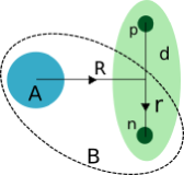
Figure 1: Coordinates involved in the $A$($d$,$p$)$B$ reactions: $\mathbf{r}$ is the radius-vector connecting the neutron and proton in the incident deuteron d, and $\mathbf{R}$ is the radius-vector connecting the deuteron and the target A centres of mass.

In this case, as shown in [7], it is convenient to expand the $\Psi_{\mathbf{k}_{d}}^{(+)}(n,p)$ scattering state in a Weinberg basis [17, 18]

$$\Psi_{\mathbf{k}_{d}}^{(+)}(n,p)=\sum_{i=0}^{\infty}\phi^{W}_{i}(\mathbf{r})\chi_{i}^{W(+)}(\mathbf{R}),$$ (2)

with Weinberg eigenstates $\phi^{W}_{i}$ and components $\chi_{i}^{W(+)}$ related to $\Psi_{\mathbf{k}_{d}}^{(+)}(n,p)$ by

$$\chi_{i}^{W(+)}(\mathbf{R})=-\frac{\langle\phi^{W}_{i}|V_{np}|\Psi_{\mathbf{k}_{d}}^{(+)}(n,p)\rangle}{\langle\phi^{W}_{i}|V_{np}|\phi^{W}_{i}\rangle},$$ (3)

where in this equation the notation $\langle\dots\rangle$ means integration over $\mathbf{r}$ only.

The validity of the ADWA is based on the accuracy of two observations.

(i) A detailed study in [19] showed that for many reactions of physical interest the matrix element in (1) is dominated by the $i=1$ term in the expansion (2). Using the fact that the $i=1$ Weinberg state is just the deuteron ground state $\Psi_{d}$ and the special orthogonality property of Weinberg states [7] we find

$$\chi_{1}^{W(+)}(\mathbf{R})=-\frac{\langle\Psi_{d}|V_{np}|\Psi_{\mathbf{k}_{d}}^{(+)}(n,p)\rangle}{\langle\Psi_{d}|V_{np}|\Psi_{d}\rangle}.$$ (4)

Consistent with this result the ADWA ignores all explicit contributions to $T_{dp}$ with $i\neq 1$.

(ii) In the ADWA the further approximation is made of ignoring the coupling between different Weinberg components, in which case the $\chi_{1}^{W(+)}(\mathbf{R})$ becomes $\chi^{\rm ADWA}(\mathbf{R})$ and is given exactly by the solution of the equation

$$\left[T_{R}+V_{\rm ADWA}(\mathbf{R})-E^{+}_{d}\right]\chi^{\rm ADWA}(\mathbf{R})=0,$$ (5)

where $E^{+}_{d}$ is the deuteron incident energy in the system c.m. frame, $T_{R}$ is the kinetic energy operator associated to $R$, and adiabatic distorted potential is given in [7] by

$$V_{\rm ADWA}(\mathbf{R})=\frac{\langle\Psi_{d}|V_{np}(\mathbf{r})V_{Ad}(\mathbf{R},\mathbf{r})|\Psi_{d}\rangle}{\langle\Psi_{d}|V_{np}(\mathbf{r})|\Psi_{d}\rangle}.$$ (6)

The ADWA potential depends on the deuteron wave function $\Psi_{d}(\mathbf{r})$, the $n$–$p$ interaction $V_{np}(\mathbf{r})$, and the interaction between the target $A$ and the deuteron components $V_{Ad}(\mathbf{R},\mathbf{r})=V_{nA}(\mathbf{R}+\frac{1}{2}\mathbf{r})+V_{pA}(\mathbf{R}-\frac{1}{2}\mathbf{r})$. In the zero-range limit for $V_{np}$ this reduces to the Johnson-Soper potential $V_{\rm ADWA}(\mathbf{R})=V_{nA}(\mathbf{R})+V_{pA}(\mathbf{R})$ [6].

In this paper we study the validity of (i) and (ii) for the special case that $V_{np}$ is the Yamaguchi rank-1 separable interaction [20]

$$V_{np}=-|f_{np}\rangle\langle f_{np}|,$$ (7)

where

$$\langle\mathbf{r}|f_{np}\rangle=N_{1}\exp(-\beta r)/r.$$ (8)

where $N_{1}$ and $\beta$ are chosen to give the correct deuteron binding energy $\epsilon_{d}$ and give a good fit to the low energy $n-p$ $s$-wave scattering.

2.2 First order perturbation to the adiabatic potential for Yamaguchi interaction

A feature of rank-1 separable potentials is that step (i) is exact because then in $T_{dp}$

$$V_{np}\Psi_{\mathbf{k}_{d}}^{(+)}(n,p)=-|f_{np}\rangle\langle f_{np}|\Psi_{\mathbf{k}_{d}}^{(+)}(n,p),$$ (9)

and the right-hand-side of Eq. (4) reduces to

$$-\frac{\langle\Psi_{d}|V_{np}|\Psi_{\mathbf{k}_{d}}^{(+)}(n,p)\rangle}{\langle\Psi_{d}|V_{np}|\Psi_{d}\rangle}=\frac{\langle f_{np}|\Psi_{\mathbf{k}_{d}}^{(+)}(n,p)\rangle}{\langle f_{np}|\Psi_{d}\rangle}.$$ (10)

Hence, Eq. (9) can be written

$$V_{np}\Psi_{\mathbf{k}_{d}}^{(+)}(n,p)=V_{np}|\Psi_{d}\rangle\chi^{\mathrm{eff}}(\mbox{\boldmath$R$}),$$ (11)

where

$$\chi^{\mathrm{eff}}(\mbox{\boldmath$R$})=\frac{\langle f_{np}|\Psi_{\mathbf{k}_{d}}^{(+)}(n,p)\rangle}{\langle f_{np}|\Psi_{d}\rangle}.$$ (12)

A second feature of the rank-1 model $V_{np}$ is that, as demonstrated in [3], an effective deuteron-target distorting potential that generates $\chi^{\mathrm{eff}}(\mbox{\boldmath$R$})$ exactly and hence goes beyond $V_{\rm ADWA}$ can be derived. A perturbative approach [3] to the calculation of this effective distorting potential is described in the next Section.

The choice of $V_{np}$ interaction is found to have a small impact on $(d,p)$ cross sections [21, 22, 23, 24], so we follow [3] and use the Yamaguchi rank-1 separable $n$-$p$ potential with parameters that give the corrrect binding energy of the deuteron, its root-mean-squared radius and the asymptotic normalization constant (ANC). The Yamaguchi ground state wave function is identical to the Hulthén deuteron wave function that reads [25, 26]

$$\Psi_{d}(\mathbf{r})=N_{0}\frac{e^{-\alpha r}-e^{-\beta r}}{r},$$ (13)

where $\alpha=\sqrt{2\mu_{d}\epsilon_{d}}/\hbar$ with $\mu_{d}$ being the reduced mass of the $n$-$p$ system, $|\epsilon_{d}|=2.2$ MeV, $\beta=6.255\alpha$ and $N_{0}$ normalizes the deuteron wave function to unity.

The s-wave scattering wave function of energy $E_{k}=\hbar^{2}k^{2}/\mu_{d}$ generated by the Yamaguchi potential is given by (see A)

$$\chi_{l=0}(k,r)=\frac{e^{i\delta_{k}}}{kr}\left[\sin(kr+\delta_{k})-\sin\delta_{k}e^{-\beta r}\right],$$ (14)

where the phase shift $\delta_{k}$ is

$$k\cot(\delta_{k})=\frac{k^{4}+(\alpha^{2}+2\alpha\beta+3\beta^{3})k^{2}-\alpha\beta^{2}(\alpha+2\beta)}{2\beta(\alpha+\beta)^{2}}.$$ (15)

We have checked that for $n$-$p$ relative energies up to 25 MeV these phase shifts are in excellent agreement (better than 1.5$\%$) with those obtained in a simplified $n$-$p$ model, given by a single Gaussian interaction with the depth of $72.15$ MeV and the range of $1.484$ fm [27], widely used in the CDCC treatment of $(d,p)$ reactions.

In the perturbative approach of [3], to the first order in $\Delta V=V_{Ad}(\mathbf{R},\mathbf{r})-V_{\rm ADWA}(\mathbf{R})$ the effective potential that generates $\chi^{\mathrm{eff}}$ is given by

$$V_{\rm eff}(\mathbf{R})\approx V_{\rm ADWA}(\mathbf{R})+G^{\rm ADWA}(E^{+}_{d}-{\bar{\epsilon}})\delta V,$$ (16)

where $V_{\mathrm{A}DWA}$ is defined in (6). The first factor of the correction term is the Green function

$$G^{\rm ADWA}(E^{+}_{d}-{\bar{\epsilon}})=\frac{1}{E^{+}_{d}-{\bar{\epsilon}}-T_{R}-V_{\rm ADWA}},$$ (17)

where the threshold ${\bar{\epsilon}}=\langle f_{np}|T_{r}|\Psi_{d}\rangle/\langle f_{np}|\Psi_{d}\rangle$ is the energy in the $n$-$p$ continuum at which the corresponding $n$-$p$ scattering states first show an oscillatory dependence on r within the range of $V_{np}$ and differ significantly from that of the deuteron ground state wave function for the same range of $\mathbf{r}$ [3]. The other factor of the corrective term in (16) is defined as

$$\delta V=\frac{\langle f_{np}|T_{r}\Delta V|\Psi_{d}\rangle}{\langle f_{np}|\Psi_{d}\rangle},$$ (18)

with $T_{r}$ the kinetic energy operator associated with $r$. For the Yamaguchi $n$-$p$ potential and Johnson-Tandy $A$-$d$ potential, we find

$$\delta V_{A}(R)=\frac{\hbar^{2}\beta^{2}}{\mu_{d}}\left(1+\frac{\alpha}{\beta}\right)\left[V_{An}(R)+V_{Ap}(R)-V_{\rm ADWA}(R)\right].$$ (19)

The effective distorted wave $\chi^{\rm eff}(\mathbf{R})$ is then obtained solving the non-homogeneous integral-differential Schrödinger equation

$$\left[T_{R}+V_{C}(R)+V_{\rm ADWA}(R)-E^{+}_{d}\right]\chi^{\rm eff}(\mathbf{R})=-s(\mathbf{R})$$ (20)

with the source term

$$s(\mathbf{R})=\int G^{\rm ADWA}(\mathbf{R},\mathbf{R}^{\prime})\delta V_{A}(\mathbf{R}^{\prime})\chi^{\rm eff}(\mathbf{R}^{\prime})d\mathbf{R}^{\prime}.$$ (21)

Equation (20) also involves the deuteron-target Coulomb interaction potential $V_{C}(R)$. As in all $(d,p)$ calculations we use the Coulomb potential of a uniformly-charged sphere for $V_{C}$ with the Coulomb radius of $R_{C}=1.3\cdot A^{1/3}$ fm, where $A$ the target mass number.

3 Numerical aspects of perturbative calculation

In this section we provide important details of the $\chi^{\rm eff}$ calculation. The calculated wave function is then read in as an input by computer code TWOFNR [28] and used to evaluate the $(d,p)$ $T$-matrix and the corresponding corrected cross sections.

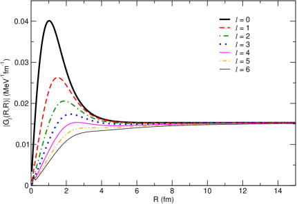
Figure 2: Absolute value of diagonal Green’s function, for partial waves up to $l=6$, calculated for $d+^{10}$Be system at the incident deuteron energy of 40.9 MeV.

3.1 Evaluation of the Green function

The effective potential $V_{\rm eff}$ involves a Green function that can be calculated using the partial-waves expansion [29]

$$G^{\rm ADWA}_{l}(R,R^{\prime})=-\frac{2\mu}{\hbar^{2}\kappa}\frac{{\cal G}^{(1)}_{l}(\kappa R_{<}){\cal G}^{(2)}_{l}(\kappa R_{>})}{{\cal W}_{l}},$$ (22)

where $\mu$ is the $A$-$d$ reduced mass, $\kappa=\sqrt{2\mu(E^{+}_{d}-{\bar{\epsilon}})/\hbar^{2}}$, and ${\cal G}^{(1)}_{l}$ and ${\cal G}^{(2)}_{l}$ are linearly independent solutions of the equation

$$\left[T_{l}+V_{C}(R)+V_{\rm ADWA}(R)-(E^{+}_{d}-{\bar{\epsilon}})\right]{\cal G}_{l}(R)=0$$ (23)

with the kinetic energy operator in the partial wave $l$,

$$T_{l}=-\frac{\hbar^{2}}{2\mu}\frac{d^{2}}{dR^{2}}+\frac{\hbar^{2}}{2\mu}\frac{l(l+1)}{R^{2}}.$$ (24)

The quantity ${\cal W}_{l}$ in (22) represents the Wronskian of ${\cal G}^{(1)}_{l}$ and ${\cal G}^{(2)}_{l}$. For the Yamaguchi potential considered in this work the threshold energy, calculated in [30] using the Hulthén wave function, is ${\bar{\epsilon}}=114$ MeV. Note that this value is strongly model dependent [31]: for other choices of the $n$-$p$ interaction it would be different but the perturbative formalism would change, too. Since most modern experiments are performed at $E^{+}_{d}<{\bar{\epsilon}}$ we will restrict ourselves by considering such cases only. The corresponding functions ${\cal G}^{(1,2)}_{l}$ satisfy boundary conditions ${\cal G}^{(1)}_{l}(R)\sim R^{l+1}$ near $R\approx 0$ and ${\cal G}^{(2)}_{l}(R)=W_{-\eta,l+1/2}(2\kappa R)$ as $R\rightarrow\infty$. Here, $W$ is the Whittaker function [32] with Sommerfeld parameter $\eta=Ze^{2}/(4\pi\epsilon_{0}\hbar v)$, $Ze$ target charge and $v$ incident velocity, so that the Green function decays exponentially at $R$ outside the range of $\Delta V$ and $V_{\rm ADWA}$. We have calculated ${\cal G}^{(1)}_{l}$ and ${\cal G}^{(2)}_{l}$ from (23) using finite difference method and we checked that the diagonal Green function convergence to the same constant value $|G^{\rm ADWA}_{l}(R,R)|\rightarrow\mu/(\hbar^{2}\kappa)$ for all partial waves at large $R$, as shown in figure 2.

Before going further we should note that for large deuteron incident energies, when $E^{+}_{d}>\bar{\epsilon}$, the ${\cal G}^{(2)}_{l}$ has a different boundary condition, ${\cal G}^{(2)}_{l}(R)\sim F_{l}(\kappa R)-iG_{l}(\kappa R)$, defined by the regular and irregular Coulomb functions $F_{l}$ and $G_{l}$ respectively [32]. This Green’s function, and the corresponding perturbative correction to the effective potential, behaves asymptotically like an oscillating outgoing wave with wave number $\kappa$.

3.2 Evaluation of the distorted wave

To determine the effective distorted waves $\chi^{\rm eff}_{l}$, needed in the calculation of the ($d$,$p$) amplitude, we solve (20) with an iterative method for each partial wave $l$, as suggested e.g. in [33]. We assume that the radial distorted wave in the partial-wave expansion of $\chi^{\rm eff}(\mathbf{R})$ is given by $\chi^{\rm eff}_{l}(R)\equiv u^{\rm eff}_{l}(R)/R=u^{(n\rightarrow\infty)}_{l}(R)/R$ and $u^{(n)}_{l}$ is found from solution of the iterative problem

$$\left[T_{l}+V_{C}(R)+V_{\rm ADWA}(R)-E_{d}\right]u^{(n+1)}_{l}(R)=$$

$$-\int_{0}^{+\infty}G^{\rm ADWA}_{l}(R,R^{\prime})\delta V_{A}(R^{\prime})u^{(n)}_{l}(R^{\prime})dR^{\prime}.$$ (25)

The first iteration of this equation solves the homogemeous ADWA equation for $u^{(1)}_{l}$ by setting $u^{(0)}_{l}$ in the r.h.s.  of (25) to zero. Then using $u^{(1)}_{l}$ in the r.h.s. we obtain $u^{(2)}_{l}$. Repeating this process several times we arrive at a converged solution for $u^{\rm eff}_{l}$. The convergence is obtained in less than $10$ iterations, with an accuracy of the first one being more than 95%. The typical computational time is a couple of seconds, when $40$ partial waves are included. In these calculations we used finite-difference Numerov or Runge-Kutta methods and imposed the boundary conditions of $u^{(n)}_{l}(0)=0$ and $u^{(n+1)}_{l}(R_{\max})=u^{(n)}_{l}(R_{\max})$. We determined the $S$-matrix elements $S_{l}$ from matching the normalization of the distorted wave $u^{(n)}_{l}$ at large distances to $\frac{i}{2}\left(H_{l}^{*}-S_{l}H_{l}\right)$, where $H_{l}=G_{l}+iF_{l}$ is a combination of regular and irregular Coulomb functions [29, 32].

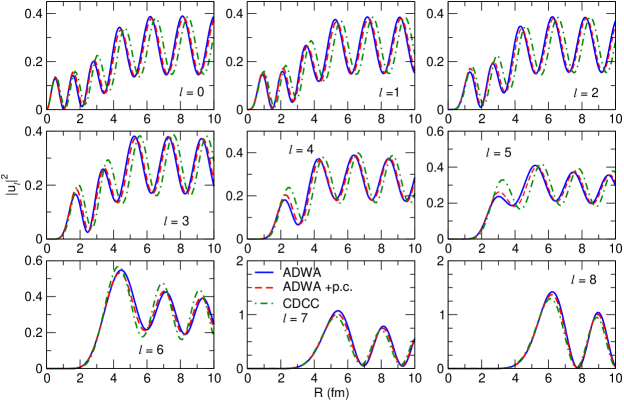
Figure 3: ADWA distorted waves (solid lines) compared to the distorted waves $u^{\rm eff}_{l}$ obtained with perturbative correction (p.c.) (dashed lines) for $d$+¹⁰Be scattering at $E_{d}=40.9$ MeV shown for partial waves $\ell\leq 8$.

To check the quality of the solution for $u^{\rm eff}_{l}$ we used an equivalent way of solving (3.2), which is provided by the system of the coupled equations

$$\left[T_{l}+V_{C}+V_{\rm ADWA}-E^{+}_{d}\right]u_{l}^{\rm eff}(R)=C_{l}u_{l}^{(\rm a)}(R)$$ (26)

$$\left[T_{l}+V_{C}+V_{ADWA}-(E^{+}_{d}-\bar{\epsilon})\right]u_{l}^{(\rm a)}(R)=C_{l}^{-1}\delta V(R)u_{l}^{\rm eff}(R),$$

where $u_{l}^{(\rm a)}$ is an auxiliary function with the boundary conditions of $u_{l}^{(\rm a)}(0)=0$ and $u_{l}^{(\rm a)}(R_{\max})\sim W_{-\eta,l+1/2}(2\kappa R_{\max})$ while $C_{l}$ is an arbitrary constant (fixed here to $1$ MeV). This system could be derived by introducing the function $u_{l}^{(\rm a)}=-C_{l}^{-1}s_{l}$, with $s_{l}$ being the radial part of the source term defined in (21), and making use of the property of the Green’s functions

$$\left[T_{l}-V_{C}(R)-V_{\rm ADWA}(R)-(E^{+}_{d}-{\bar{\epsilon}})\right]G^{\rm ADWA}_{l}(R,R^{\prime})=\delta(R,R^{\prime}).$$ (27)

We solved these coupled equations using the $R$-matrix code developed by P. Descouvemont [34]. The resulting functions $u^{\rm eff}_{l}$ were in excellent agreement with those obtained by iterative solution of (3.2). An example of $u^{\rm eff}_{l}$ is shown in figure 3 for the $d+^{10}$Be system at $E_{d}=40.9$ MeV for a few partial waves, up to $\ell=8$, using global parameterisation CH89 [35] for $n$-¹⁰Be and $p$-¹⁰Be optical potentials.

Figure 3 shows that the character of the distorted waves changes after $\ell=6$, which corresponds to the product $kR_{N}$ of the deuteron momentum $k\sim 2$ fm^-1 and nuclear radius $R_{N}\sim 3$ fm. Distorted waves with $\ell<6$ have noticeable presence in the nuclear interior and their imaginary parts significantly contribute to the absolute values $|u_{l}|^{2}$. At $\ell>6$ all the distorted waves are practically zero within the range $0<R<R_{N}$ and they also become real. We also notice that perturbative correction for $\ell>kR_{N}$ is practically negligible in the internal region. On close examination, we find that absolute value of $|u_{l}|^{2}$ in their maxima are affected by perturbative correction by less then 5$\%$, 2$\%$ and 1$\%$ at $\ell=7$, 8 and 10. The influence on S-matrix element is the largest at $\ell\sim kR_{N}$, around 8%, for partial waves with $\ell<kR_{N}$ it does not exceed 5% and quickly becomes negligible with increasing $\ell$. The S-matrix elements are shown in Table 1. To understand this result we go back to (20) with the source term (21). The integrand of the source term contains the product of the correction potential $\delta V_{A}$, which is concentrated on the nuclear surface $R_{N}$, and the distorted wave that starting from some $\ell$ is zero everywhere within $R_{N}$. Therefore, for $l>kR_{N}$ the source term becomes close to zero leading to negligible influence from the perturbative corrections. We have observed the same trend in all other cases studied in this work. This observation should have certain consequences for the $(d,p)$ cross sections calculations. We can expect that the cross sections calculated with $\ell>kR_{N}$ will not be affected by the perturbative corrections while those that retain $\ell\leq kR_{N}$ only will show maximum sensitivity to them. The final conclusion about the role of perturbative corrections will therefore depend on relative contribution of the lowest partial waves to the $(d,p)$ cross section. Below we check this conjecture by using $u^{\rm eff}_{l}$ to calculate $(d,p)$ cross sections for different ranges of $\ell$ for a variety of targets and deuteron incident energies.

$l$		0	1	2	3	4	5
$|S_{l}|$	${\rm ADWA}$	0.2421	0.2320	0.2229	0.1988	0.1828	0.1488
	${\rm ADWA+p.c.}$	0.2298	0.2219	0.2149	0.1971	0.1879	0.1554
$l$		6	7	8	9	10	11
$|S_{l}|$	${\rm ADWA}$	0.1867	0.6059	0.8369	0.9320	0.9709	0.9874
	${\rm ADWA+p.c.}$	0.1917	0.5594	0.7980	0.9087	0.9580	0.9805

Table 1: Absolute value of the $S$-matrix element $|S_{l}|$ in partial wave $\ell$ calculated for $d+^{10}$Be scattering at $E_{d}=40.9$ MeV in ADWA without and with perturbatice correction (p.c.).

4 Perturbative calculations versus ADWA and CDCC

All $(d,p)$ calculations presented in this section were performed using global nucleon optical potentials in the entrance and exit channels, given by either the CH89 [35] or KD02 [36] and neglecting spin-orbit interaction in the deuteron channel. To describe the bound state wave function of the transferred neutron we used a two-body Woods-Saxon central potential model of a standard geometry (radius $r_{0}=1.25$ fm and diffuseness $a=0.65$ fm), adjusting its depths to reproduce the neutron separation energy of the relevant state. The spectroscopic factor was assumed to be one everywhere. We compare the $(d,p)$ angular distributions obtained in perturbative model to those given by uncorrected ADWA theory with the Johnson-Tandy potential. To understand if perturbative correction treatment of $(d,p)$ reactions is sufficient to include significant part of the $n$-$p$ continuum effects, we compare the corresponding cross sections to the CDCC predictions made with the help of the computer code FRESCO [37]. We point out that the rank-1 Yamaguchi $n$-$p$ potential is nonlocal while FRESCO has been developed for local potentials only. Therefore, additional efforts are needed to perform such calculations. We will describe important details of the CDCC calculations before showing any numerical results.

4.1 Details of the CDCC calculations

The CDCC scattering wave function has the structure

$$\Psi^{\mathrm{CDCC}(+)}_{\mathbf{k}_{d}}(n,p)=\sum_{b}\phi_{b}(r)\chi_{b}(\mathbf{R})+\dots,$$ (28)

where the sum is over a set of discretized bound and continuum s-wave eigenstates of $V_{np}$, and the dots indicate non-s-wave continuum states that may contribute to the CDCC coupled equations that determine the $\chi_{b}(\mathbf{R})$ but do not contribute to $T_{dp}$ because of the s-wave nature of $|f_{np}\rangle.$ The functions $\chi_{b}(\mathbf{R})$ are obtained as solutions of coupled differential equations with the coupling matrix elements $V^{\lambda}_{ii^{\prime}}(R)=\langle\phi_{i^{\prime}}||Y^{*}_{\lambda}(V_{nA}+V_{pA})||\phi_{i}\rangle$, where $\phi_{i}$ is either a deuteron ground state wave function or a continuum bin with orbital momentum $l_{i}$. We calculated these matrix elements externally and then read them into FRESCO. In these calculations the deuteron ground state wave function was taken from the Hulthén model while $s$-wave continuum bins $\phi_{i}$ were constructed using Yamaguchi wave functions given by (14). For other $n$-$p$ orbital momenta $l_{i}$ we used spherical Bessel functions $j_{l}(kr)$, representing plane waves, to obtain continuum bins.

We show the coupling potentials $V^{\lambda}_{ii^{\prime}}(R)$ for the lowest $s$-, $p$- and $d$-waves in figure 4, for the case of the $d+^{10}$Be scattering at $E_{d}=40.9$ MeV using nucleon optical potentials $V_{An}$ and $V_{Ap}$ from the Woods-Saxon global optical potential parameterisation CH89 [35]. The $n$-$p$ continuum bins span the energy interval between 0 and 1 MeV. The figure shows that the diagonal ground state $s$-wave matrix element is dominant in the nuclear interior and the coupling between the deuteron ground state and the $p$- and $d$-wave continuum bins is between three and two orders of magnitude smaller in this area. Also, the coupling involving the first $s$-wave continuum bin are two or three time bigger than those involving $p$- and $d$-wave. This suggests that including $p$- and $d$-waves into the coupling scheme will not be important. We have confirmed this later by running the CDCC calculations with $s$-waves only and with including $p$- and $d$-wave continuum. As expected, the results of such two sets of calculations did not differ.

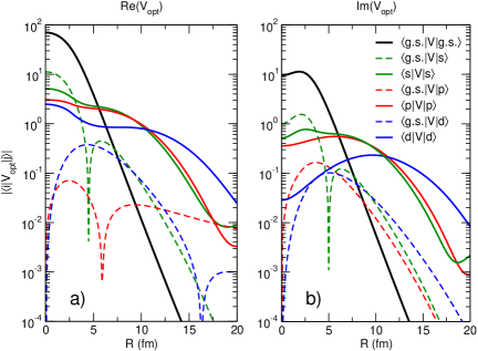
Figure 4: The absolute value of the monopole parts of the coupling potentials $V^{0}_{ii}(R)$ and the coupling potentials connecting deuteron ground state with the lowest $s$-, $p$- and $d$-wave continuum bins in the Yamaguchi separable rank-1 $n$-$p$ model. The calculations are shown for real $(a$) and imaginary $(b)$ parts of the optical potentials separately.

Unlike in calculations with local $n$-$p$ potentials, where transitions occur explicitly between all continuum bins, the contribution of the CDCC wave function to the amplitude $T_{dp}$ is determined, from (11) and (12), by the quantity

$$V_{np}\Psi_{\mathbf{k}_{d}}^{(+)}(n,p)=(V_{np}|\Psi_{d}\rangle)\sum_{b}\frac{\langle f_{np}|\phi_{b}\rangle}{\langle f_{np}\mid\Psi_{d}\rangle}\chi_{b}(\mathbf{R}).$$ (29)

The sum over $b$ represents exactly the expansion over the CDCC basis of the first Weinberg component, as discussed first in [19]. The calculations with the first component only are equivalent to those involving well-known one-channel distorted-wave Born approximation. We have calculated the weight factors (or expansion coefficients) $\frac{\langle f_{np}|\phi_{b}\rangle}{\langle f_{np}\mid\Psi_{d}\rangle}$ using the s-wave scattering states of the Yamaguchi potential that appear in the $\phi_{b}$ and then, using the FRESCO output for $\chi_{b}(\mathbf{R})$, carried out the summation over $b$ to obtain the first Weinberg component. Then, similar to [19], this component was read back into FRESCO. The zero-range option for evaluating the $(d,p)$ amplitude was chosen with the standard value $D_{0}=-122.50$ MeV fm^3/2.

4.2 $(d,p)$ cross sections results

We have tested the perturbative correction on a variety of $(d,p)$ reactions, selecting different targets and different separation energies and quantum numbers of transferred neutron. We have chosen beam energies in the intermediate range, to avoid necessity for including contributions from closed channels. Therefore, all the calculations presented below were carried out at deuteron energies above 40 MeV. Details on the separation energies $S_{n}$ and quantum numbers for each system, as well as the corresponding beam energy and the global parametrisation used are presented in table 2.

Target	$S_{n}$ (MeV)	nlj	$E_{d}$ (MeV)	Global param.
10Be	0.504	$2s_{1/2}$	40.9; 71	CH89
48Ca	5.146	$2p_{3/2}$	56; 100	CH89
40Ca	8.363	$1f_{7/2}$	56	KD02
55Ni	16.643	$1f_{7/2}$	40	KD02
40Ca [14]	0.1	$2s_{1/2}$	40	KD02

Table 2: Parameters of the n-target systems used in the calculations. $S_{n}$ is the neutron separation energy in MeV, nlj are the quantum number describing the ground state of the nucleus in the outgoing channel. The targets are in their $0^{+}$ ground state, except for ⁵⁵Ni, which has a $7/2^{-}$ ground state. $E_{d}$ are the deuteron beam energies in MeV considered in each case. We also specify the global parameterisation used in each calculation.

We start examining the $(d,p)$ cross sections results with the ¹⁰Be($d,p)^{11}$Be reaction at $E_{d}=40.9$ and $71$ MeV. In the first case, the distorted waves have already been discussed in section 3.2. Our calculations with different ranges of partial waves $\ell$, included in description of the deuteron channel, have confirmed the conjecture made in that section that the influence of the perturbative correction on the cross sections comes from the partial waves with $\ell\leq\kappa R_{N}$ only. For a particular choice of the ¹⁰Be($d,p)^{11}$Be reaction the contribution from the low partial waves is noticeable, with the main contribution coming from $\ell\sim\kappa R_{N}$. The effect of the perturbation on the cross section is compared to the ADWA result in figure 5, for both beam energies, as dashed and solid lines respectively. The benchmark CDCC calculations are shown as dot-dashed lines. In both cases, including perturbative corrections affects mainly the second maximum in a region between 20-50 degrees, with 20-30$\%$ increase of the cross sections. We proceed with the ⁴⁸Ca$(d,p)^{49}$Ca reaction, studied for $E_{d}=56$ and 100 MeV. Figure 6 compares the ADWA, calculated without and with perturbative corrections, with the CDCC predictions. Similar to the ¹⁰Be$(d,p)^{11}$Be case, the perturbative description is not sufficient to get closer to the CDCC results in the angular ranges where non-adiabatic effects are not negligible. The perturbation brings the ADWA result closer to the CDCC at forward angles in the cases of ⁵⁵Ni$(d,p)^{56}$Ni reaction at 40 MeV, in figure 7, and ⁴⁰Ca$(d,p)^{41}$Ca reaction at 56 MeV, shown in figure 8. However, it is not sufficient at higher angles.

In most of the cases considered above, ADWA and CDCC calculations differ considerably, and thus could be considered non-adiabatic, as already shown e.g. by [12, 13]. While at forward peak the non-adiabatic effects are of the order of 30$\%$ in most of the cases, at the second peak they almost double the cross section. In these situations, the effect of the perturbative correction on the second peak is not sufficient to account for this change. By comparing perturbative ADWA and CDCC calculations performed in different fixed ranges of $\ell$ we conclude that perturbative corrections are not sufficient at small $\ell$ as well.

Other cases where the ADWA and CDCC descriptions differ stronger were identified in [14], where ADWA validity was tested systematically for a variety of cases with different masses, charges, binding energies, angular momenta and beam energies. Among the typical situations in which the ADWA failed significantly highlighted in this study, the one with small $S_{n}$ and relatively high incident energies was indicated. This was represented by the fictitious ⁴⁰Ca($d$,$p$)⁴¹Ca(2$s_{1/2}$) with $E_{d}=40$ MeV and $S_{n}=0.1$ MeV reaction (figure 5a of [14]). We have reproduced the ADWA calculation from [14] and compared it with the perturbative calculation and a CDCC benchmark calculation in figure 9. The perturbative correction plays a similar role, as the cases considered above. However, the perturbative calculation still differs from the CDCC.

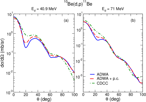
Figure 5: ¹⁰Be($d$,$p$)¹¹Be differential cross section with respect to the c.m. angle for the calculations with and without the perturbative correction (dashed and solid lines respectively) for $E^{lab}_{d}=40.9$ and $71$ MeV. The CDCC calculations are shown as dot-dashed lines. Global parameterisation CH89 was used in these calculations.

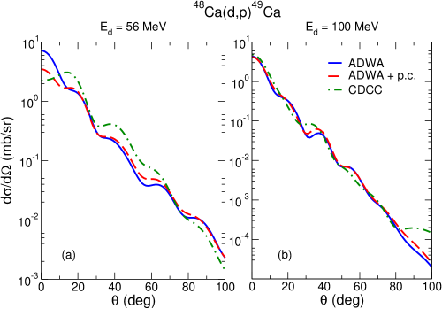
Figure 6: ⁴⁸Ca($d$,$p$)⁴⁹Ca differential cross section with respect to the c.m. angle for the calculations with and without the perturbative correction for $E^{lab}_{d}=56$ and $100$ MeV (dashed and solid lines respectively). CDCC calculations are shown by dotted-dashed lines. Global parameterisation CH89 was used in these calculations.

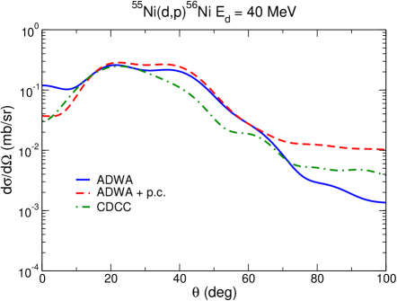
Figure 7: ⁵⁵Ni($d$,$p$)⁵⁶Ni differential cross section with respect to the c.m. angle for the calculations with and without the perturbative correction for $E^{lab}_{d}=40$ MeV (dashed and solid lines respectively). CDCC calculations are shown by dotted-dashed lines. The global parameterisation KD02 was used for nucleon optical potentials in the entrance and exit channels.

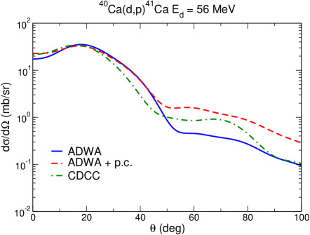
Figure 8: ⁴⁰Ca($d$,$p$)⁴¹Ca differential cross section with respect to the c.m. angle for the calculations with and without the perturbative correction for $E^{lab}_{d}=56$ MeV (dashed and solid lines respectively). CDCC calculations are shown by dotted-dashed lines. The global parameterisation KD02 was used for nucleon optical potentials in the entrance and exit channels.

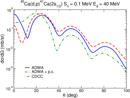
Figure 9: Differential cross section with respect to the c.m. scattering angle for a case selected from systematical study of Chazono et al [14]. Solid lines represent the ADWA result while the CDCC calculation is shown as dot-dashed lines. The result including perturbative correction to the ADWA is shown by dashed lines. The global parameterisation KD02 was used for nucleon optical potentials in the entrance and exit channels.

		ADWA+p.c./ADWA		ADWA+p.c./CDCC		ADWA/CDCC
Target	$E_{d}$ (MeV)	1st peak	2nd peak	1st peak	2nd peak	1st peak	2nd peak
10Be	40.9	0.876	1.228	0.905	0.818	1.033	0.666
	71	1.018	1.341	0.802	0.697	0.788	0.520
48Ca	56	0.485	1.088	1.552	0.568	3.200	0.522
	100	0.965	1.297	0.868	0.886	0.899	0.683
55Ni	40	0.310	1.101	1.225	1.151	3.956	1.045
40Ca	40	0.261	1.230	0.705	0.995	2.703	0.809
	56	1.314	0.931	1.054	0.956	0.802	1.027

Table 3: The target nucleus, deuteron incident energy (in MeV) and ratios of the corrected ADWA cross section to those calculated in ADWA and CDCC in the first forward peak at 0 degrees and in the second peak at $\theta>25$ deg. The ratios of the ADWA to CDCC cross sections in the two peaks are given in the last two columns. Note that in the case of ⁴⁰Ca target and $E_{d}=40$ MeV, the orbital and binding energy of the final state are changed according to [14].

5 Summary

We have presented a numerical assessment for the first order perturbative correction to the ADWA description of ($d$,$p$) reactions that has been proposed in [3] for a class of separable rank-1 $n$-$p$ potentials. This correction arises due to additional nonlocal contribution to the optical potential to be used to calculate deuteron-target distorted waves. The corrected distorted waves were evaluated externally and then used as input for the cross section calculations performed with TWOFNR’s help. The first Weinberg component, representing exact CDCC calculations with (nonlocal) rank-1 Yamaguchi $n$-$p$ potential, was constructed from the CDCC solutions for deuteron-target scattering waves, which were obtained by running FRESCO with externally read-in coupling matrix elements in the Yamaguchi basis. FRESCO was also employed to read in this component and provide the CDCC cross sections.

Numerical calculations have shown that perturbative corrections affect mainly the partial waves with $\ell\leq\kappa R_{N}$ while higher $\ell$’s remain unaffected so that the overall influence of this correction depend on the relative contribution of lower and higher partial waves to the $(d,p)$ amplitude. The first order perturbative correction has been applied to ¹⁰Be($d$,$p$), ^40,48Ca($d$,$p$) and ⁵⁵Ni($d$,$p$) reactions for several beam energies large enough to neglect contributions from closed channels. Overall, our results indicate corrections ranging from $2-25\%$ at forward angles to up to $40-50$% at scattering angles higher than $20$ degrees. The ratios of the ADWA+p.c. cross sections to ADWA and CDCC, shown in table 3, give an idea of how much spectroscopic factors and asymptotic normalization coefficients would change if perturbative calculation replaced the ADWA or CDCC in the analysis of experimental $(d,p)$ data. These ratios have been evaluated at 0 deg (1st peak), and at the first maximum of each differential cross section individually (2nd peak). The perturbative correction works better at higher angles, and at forward angles it sometimes brings the cross section closer to the CDCC predictions.

In general, the first-order perturbative corrections as proposed in [3], are not sufficient to bring the $(d,p)$ ADWA cross sections into agreement with exact three-body results. However, we should note that the approach of Ref. [3] is based on several assumptions, related to Green’s functions properties, whose validity has not been thoroughly investigated. Further work should explore extension of the first-order perturbation theory beyond these assumptions. The interest for pursuing in this direction is motivated by difficulties in generalizing the CDCC approach to include nonlocal nucleon-target optical potentials, as well as clarifying the role of induced three-body effects in $(d,p)$ reactions beyond ADWA. First-order perturbation theory could advance our knowledge of these not yet understood physical problems.

Appendix

Appendix A Scattering states for the Yamaguchi rank-1 separable potential [20].

Neutron-proton scattering states $\mid\chi_{\mbox{\boldmath$k$}}\rangle$ in the potential $V$ are defined as the limit $\epsilon\rightarrow 0+$ of the states

$$\mid\chi^{(\epsilon)}_{\mbox{\boldmath$k$}}\rangle=(2\pi)^{3/2}\frac{\imath\epsilon}{(E_{k}+\imath\epsilon-T_{r}-V)}\mid\mbox{\boldmath$k$}\rangle,$$ (30)

where

$$T_{r}=\frac{\mbox{\boldmath$p$}^{2}}{\mu_{d}},\,\,\,\langle\mbox{\boldmath$r$}\mid\mbox{\boldmath$k$}\rangle=\frac{\exp(\imath\mbox{\boldmath$r$}\cdot\mbox{\boldmath$k$})}{(2\pi)^{3/2}},\,\,E_{k}=\frac{\hbar^{2}k^{2}}{\mu_{d}}.$$ (31)

and $\mu_{d}$ is the neutron-proton reduced mass. The state $\mid\chi^{(\epsilon)}_{\mbox{\boldmath$k$}}\rangle$ also satisfies

$$\mid\chi^{(\epsilon)}_{\mbox{\boldmath$k$}}\rangle=(2\pi)^{3/2}\mid\mbox{\boldmath$k$}\rangle+\frac{1}{(E_{k}+\imath\epsilon-T_{r})}V\mid\chi^{(\epsilon)}_{\mbox{\boldmath$k$}}\rangle,$$ (32)

For a rank-1 separable potential

$$V=-\mid f\rangle\langle f\mid,$$ (33)

(32) becomes

$$\mid\chi^{(\epsilon)}_{\mbox{\boldmath$k$}}\rangle=(2\pi)^{3/2}\mid\mbox{\boldmath$k$}\rangle-\frac{1}{(E_{k}+\imath\epsilon-T_{r})}\mid f\rangle\langle f\mid\chi^{(\epsilon)}_{\mbox{\boldmath$k$}}\rangle,$$ (34)

and hence

$$\langle f\mid\chi^{(\epsilon)}_{\mbox{\boldmath$k$}}\rangle=(2\pi)^{3/2}\frac{\langle f\mid\mbox{\boldmath$k$}\rangle}{(1+\langle f\mid\frac{1}{(E_{k}+\imath\epsilon-T_{r})}\mid f\rangle)}.$$ (35)

Substituting (35) into (34) gives the explicit expression for $\mid\chi^{(\epsilon)}_{\mbox{\boldmath$k$}}\rangle$

$$\mid\chi^{(\epsilon)}_{\mbox{\boldmath$k$}}\rangle=(2\pi)^{3/2}\left(\mid\mbox{\boldmath$k$}\rangle-\frac{1}{(E_{k}+\imath\epsilon-T_{r})}\times\frac{\mid f\rangle\langle f\mid\mbox{\boldmath$k$}\rangle}{(1+\langle f\mid\frac{1}{(E_{k}+\imath\epsilon-T_{r})}\mid f\rangle)}\right),$$ (36)

For the Yamaguchi potential

$$\langle\mbox{\boldmath$r$}\mid f\rangle=N_{1}\frac{\exp(-\beta r)}{r},$$ (37)

we find

$$\langle\mbox{\boldmath$k$}^{\prime}\mid f\rangle=\frac{4\pi N_{1}}{(2\pi)^{3/2}}\frac{1}{(\beta^{2}+k^{\prime 2})},$$ (38)

and

$$\langle f\mid\frac{1}{(E_{k}+\imath\epsilon-T_{r})}\mid f\rangle=\frac{2\pi\mu_{d}N_{1}^{2}}{\hbar^{2}\beta}\frac{1}{(k+\imath\frac{\epsilon}{2k}+\imath\beta)^{2}}.$$ (39)

A bound state $\mid\psi_{0}\rangle$ satisfies

$$\mid\psi_{0}\rangle=\frac{1}{(-\epsilon_{d}-T_{r})}V\mid\psi_{0}\rangle=\frac{1}{(\epsilon_{d}+T_{r})}\mid f\rangle\langle f\mid\psi_{0}\rangle,$$ (40)

hence if $\mid\psi_{0}\rangle\neq\mid 0\rangle$, the constants $\alpha,\beta,N_{1}$ must satisfy

$$\langle f\mid\frac{1}{(\epsilon_{d}+T_{r})}\mid f\rangle=1.$$ (41)

By putting $k=\imath\alpha$, $\epsilon_{d}=\frac{\hbar^{2}}{\mu_{d}}\alpha^{2},$ in the result (39) the condition (41) gives

$$\frac{2\pi\mu_{d}N_{1}^{2}}{\hbar^{2}\beta}\frac{1}{(\alpha+\beta)^{2}}=1.$$ (42)

Therefore if the potential $V$ does support a bound deuteron the formula (39) can be replaced by

$$\langle f\mid\frac{1}{(E_{k}+\imath\epsilon-T_{r})}\mid f\rangle=\frac{(\beta+\alpha)^{2}}{(k+\imath\frac{\epsilon}{2k}+\imath\beta)^{2}}.$$ (43)

Using these explicit formulae in (36) we find

$$\langle\mbox{\boldmath$r$}\mid\chi^{(\epsilon)}_{\mbox{\boldmath$k$}}\rangle = \exp(\imath\mbox{\boldmath$r$}\cdot\mbox{\boldmath$k$})+\frac{2\beta(\alpha+\beta)^{2}}{(k-\imath\alpha)(k-\imath\beta)^{2}(k+\imath(2\beta+\alpha))}$$ (44)

$$\times \left(\frac{\exp(\imath kr)}{r}-\frac{\exp(-\beta r)}{r}\right),$$

note that according to (44) the scattered wave has $\ell=0$ only. The coefficient of the scattered wave is the scattering amplitude $f(k,\theta)$ which in this case is independent of $\theta$ and related to the s-wave phase shift $\delta_{k}$, all other phase shifts vanish, by

$$f=\frac{\exp(\imath\delta_{k})\sin\delta_{k}}{k},$$ (45)

or equivalently

$$k\cot\delta_{k}=\imath k+\frac{1}{f}=\frac{k^{4}+(\alpha^{2}+2\alpha\beta+3\beta^{2})k^{2}-\alpha\beta^{2}(\alpha+2\beta)}{2\beta(\alpha+\beta)^{2}},$$ (46)

according to (44). The scattering length $a$ and the effective range $r_{0}$ are defined by the expansion in powers of $k$

$$k\cot\delta_{k} =-\frac{1}{a}+\frac{1}{2}r_{0}k^{2}+\dots.$$ (47)

From (46) we deduce

$$a =\frac{2(\alpha+\beta)^{2}}{\alpha\beta(\alpha+2\beta)}$$

$$r_{0} =\frac{(\alpha^{2}+2\alpha\beta+3\beta^{2}}{\beta(\alpha+\beta)^{2}}.$$ (48)

The $\ell=0$ component of the scattering wavefunction (44) can be written

$$\chi_{0}^{(+)}(k,r) =\frac{\sin(kr)}{kr}+\frac{\exp(\imath\delta_{k})\sin\delta_{k}}{k}\left(\frac{\exp(\imath kr)}{r}-\frac{\exp(-\beta r)}{r}\right)$$ (49)

$$=\frac{\exp(\imath\delta_{k})}{kr}(\sin(kr+\delta_{k})-\sin\delta_{k}\exp(-\beta r)).$$

References

References

- [1] Butler S T 1950 Phys. Rev. 80 1095–1096
- [2] Bhatia A, Huang K, Huby R, and Newns H 1952 The London, Edinburgh, and Dublin Philosophical Magazine and Journal of Science 43 485–500
- [3] Johnson R C 2014 J. Phys. G: Nucl. Part. Phys. 41 094005
- [4] Timofeyuk N and Johnson R C 2020 Progr. Part. Nucl. Phys. 111 103738
- [5] Watanabe S 1958 Nucl. Phys. 8 484–492
- [6] Johnson R C and Soper P J R 1970 Phys. Rev. C 1 976–990
- [7] Johnson R C and Tandy P 1974 Nucl. Phys. A 235 56–74
- [8] Rawitscher G H 1975 Nucl. Phys. A 241 365–385
- [9] Austern N, Iseri Y, Kamimura M, Kawai M, Rawitscher G H and Yahiro M 1987 Phys. Rep. 154 125–204
- [10] Faddeev L D 1961 Z. Eksp. Teor. Fiz. 39 1459; 1961 Sov. Phys. J. Exp. Theor. Phys. 12 1014
- [11] Austern N, Kawai M and Yahiro M 1996 Phys. Rev. C 53 314–321
- [12] Nunes F M and Deltuva A 2011 Phys. Rev. C 84 034607
- [13] Upadhyay N J , Deltuva A and Nunes F M 2012 Phys. Rev. C 85 054621
- [14] Chazono Y, Yoshida K and Ogata K 2017 Phys. Rev. C 95 064608
- [15] Johnson R C and Timofeyuk N K 2014 Phys. Rev. C 89 024605
- [16] Dinmore M J, Timofeyuk N K, Al-Khalili J S and Johnson R C 2019 Phys. Rev. C 99 064612
- [17] Weinberg S 1963 Phys. Rev. 131 440–460
- [18] Weinberg S 1964 Phys. Rev. 133 B232–B256
- [19] Pang D Y, Timofeyuk N K, Johnson R C and Tostevin J A 2013 Phys. Rev. C 87 064613
- [20] Yamaguchi Y 1954 Phys. Rev. 95 1628–1634
- [21] Holt J D, Kuo T T S and Brown G E 2004 Phys. Rev. C 69 034329
- [22] Jurgenson E D, Bogner S K, Furnstahl R J and Perry R J 2008 Phys. Rev. C 78 014003
- [23] Gómez-Ramos M and Timofeyuk N K 2018 Phys. Rev. C 98 011601(R)
- [24] Deltuva A 2018 Phys. Rev. C 98 021603(R)
- [25] Hulthén L and Laurikainen K V 1951 Rev. Mod. Phys. 23 1–9
- [26] Hulthén L and Nagel B C H 1953 Phys. Rev. 90 62–69
- [27] Yahiro M, Iseri Y, Kamimura M and Nakano M 1984 Phys. Lett. B 141 19–22
- [28] Tostevin J A University of Surrey corrected and updated version of the code twofnr (of Toyama M, Igarashi M and Kishida N) and code front,
- [29] Satchler G 1983 Direct Nuclear Reactions (Oxford: Oxford University Press)
- [30] Timofeyuk N K and Johnson R C 2013 Phys. Rev. Lett. 110 112501
- [31] Bailey G W, Timofeyuk N K and Tostevin J A 2016 Phys. Rev. Lett. 117 162502
- [32] Abramowitz M and Stegun I A 1970 Handbook of Mathematical Functions (New York: Dover)
- [33] Michel N 2009 Eur. Phys. J. A 42 523
- [34] Descouvemont P 2016 Comp. Phys. Comm. 200 199–219 .
- [35] Varner P R, Thompson W, McAbee T, Ludwig E and Clegg T 1991 Phys. Rep. 201 57
- [36] Koning A and Delaroche J 2003 Nucl. Phys. A 713 231–310
- [37] Thompson I J 1988 Comput. Phys. Rep. 7 167