Stability and convergence analysis of a domain decomposition FE/FD method for the Maxwell’s equations in time domain
M. Asadzadeh∗ and L. Beilina
Department of Mathematical Sciences, Chalmers University of Technology and University of Gothenburg, SE-42196 Gothenburg, Sweden, e-mail: mohammad@chalmers.se, larisa@chalmers.se
Abstract
Stability and convergence analysis for the domain decomposition finite element/finite difference (FE/FD) method developed in [3, 4] is presented. The analysis is designed for semi-discrete finite element scheme for the time-dependent Maxwell’s equations. The explicit finite element schemes in different settings of the spatial domain are constructed and domain decomposition algorithm is formulated. Several numerical examples validate convergence rates obtained in the theoretical studies.
1 Introduction
New computational techniques meet the needs of
industry in developing efficient computational methods to simulate
partial differential equations (PDEs). Especially,
for simulations in higher dimensions
and large computational domains. In this regard, certain
domain decomposition (DD) method
leading to efficient schemes, in numerical investigations,
has gained a lot of interest in numerical analysis community.
This variant of the DD method is the
subject of our current, and some related and ongoing, research.
This type of schemes was previously studied, e.g. in
[12, 30] for others than studied here problems.
The present work is a further development of the
DD hybrid finite element/finite difference (FE/FD)
method for time-dependent Maxwell’s equations for
electric field in non-conductive media, studied in [3, 4].
A stable, time-domain (TD), DDM scheme
for Maxwell’s equations was
proposed in [26, 27], and further verified in [13].
This method uses FDTD scheme on the, structured, FD part of the
mesh, and edge elements on unstructured part. In applications, because of
edge elements implementation, this method remains computationally expensive.
The domain decomposition FE/FD method for time-dependent
Maxwell’s equations for electric field, assuming constant dielectric
permittivity function in a finite difference domain, was
considered in [3]. This assumption
simplifies the numerical schemes in both FE
and FD domains and significantly reduces computational efforts for
implementation of the whole DD method. Modified
numerical scheme, energy estimate and numerical verifications of this
method was presented in [4]. However, the fully stability and
convergence analysis with numerical implementations, in - and -norms of the
developed FE and FD schemes, are
not presented in the above studies. We fill this gap in the present work.
More specificaly, we present stability analysis for explicit schemes
for both FEM and FDM in the DD hybrid FE/FD method.
The DDM is constructed such that FEM and FDM
coincide on the common, structured, overlapping layer between the two
subdomains. The resulting domain decomposition approach at the
overlapping layers can be viewed as a FE scheme
which avoids instabilities at the interfaces. Similar to the DD approach of [4, 5],
we decompose
the computational domain such that FEM and FDM are used in different subdomains: FDM
in simple geometry and FE in the subdomain
where more detailed information is needed about the structure of
this subdomain. This also allows application of adaptive FEM in such
subdomain, see, e.g. [2, 3, 8, 9, 10, 28, 29].
Reliability and convergence of the domain decomposition method,
studied in this work, are evident for solution of coefficient
inverse problems (CIPs) in , see,
e.g. [8, 9, 10, 28, 29]. For the case
of CIPs, the computational domain is splitted into subdomains such
that a simple discretization scheme can be used in a large region and
more refined discretization scheme is applied in smaller, however
more critical, part of the domain. In most algorithms for
solution of electromagnetic CIPs, to determine the dielectric
permittivity function inside a computational domain, a qualitative
collection of experimental measurements is necessary on it’s boundary
or in it’s neighborhood. In such cases it is convenient to condsider the numerical solution of
time-dependent Maxwell’s equations in
different subdomains with constant dielectric permittivity function
in some subdomain and non-constant in the other ones. For the
time-dependent Maxwell’s equations, the DD scheme
of [4], which is analyzed in the present work, is used
for solution of different CIPs to determine the dielectric
permittivity function in non-conductive media using simulated and
experimentally generated data, see [2, 8, 9, 10, 28, 29].
An outline of this paper is as follows. In Section 2 we introduce the
mathematical model. In Section 3 we briefly present the domain
decomposition FE/FD method and communication scheme between two methods. In
Section 4 we describe the domain decomposition FE/FD method for
solution of Maxwell’s equations and set up the finite element and
finite difference schemes. Section 5 is devoted to the stability analysis.
In Section 6, we derive optimal a priori error estimates in
finite element method for the
semi-discrete (spatial discretizations) problems. Finally, in Section 7 we present numerical
implementations that justify the theoretical investigations of the
paper. In what follows, will be a generic constant independent of all parameters, unless otherwise specifically specified, and not necessarliy the same at each occurance.
2 The mathematical model
The Cauchy problem for the
electric field ,
, , of the Maxwell’s equations, under the
assumptions that the dimensionless relative magnetic permeability of
the medium is and
the electric volume
charges are zero, is given by
(1)
where, and
are the dimensionless relative dielectric permittivity and
electric conductivity functions, respectively. , and
are the permittivity and permeability of the free space,
respectively, and is the speed of
light in free space. In this paper we consider the problem (1) in non-conductive media, i.e.
, and hence study the initial value problem
(2)
To solve the problem (2) numerically, we consider it in a bounded domain
(instead of whole ),
with boundary , and employ a split scheme on
: a hybrid, finite element/finite
difference scheme, kind of
domain decomposition, developed in [3, 4] and summarized in
Algorithm 1. More specifically, we divide the computational domain
into two subregions, and such that
and is a subset of the convex hul of
. The function
is assumed to be constant in , and bounded and smooth
in .
The communication ß
between and is arranged using an
overlapping mesh structure through a two-element thick layer around
as shown by blue and green common boundaries in Figure
1. The blue boundary is outer boundary of and inner boundary of . Similarly, the green
boundary is the inner boundary of from which the
solution is copied to the green boundary of .
The key idea with such a decomposition is to be able apply different
numerical methods in different computational domains. For the
numerical solution of (2) in we use the
finite difference method on a structured mesh. In , we
use finite elements on a sequence of unstructured meshes , with elements consisting of triangles in
and tetrahedra in , both satisfying minimal angle condition.
This approach combines the flexibility of the finite elements and the
efficiency of the finite differences in terms of speed and memory
usage and fits well for reconstruction algorithms presented below.
We assume that for some known constant , the function
satisfies
together with divergence free field , make equations in
(2) independent of each others in and so that, in ,
we just need to solve the system of wave equations:
(5)
Remark
It is well known that, for stable implementation of the finite element
solution of Maxwell’s equations, divergence-free edge elements are the
most satisfactory ones from a theoretical point of view
[21, 24]. However, the edge elements are less attractive for
solution of time-dependent problems, since a linear system of equations
should be solved at each time iteration step. In contrary, P1
elements can be efficiently used in a fully explicit finite element
scheme with lumped mass matrix [11, 14, 18]. It is also
well known that numerical solution of Maxwell’s equations using nodal
finite elements is often unstable and results spurious oscillatory
solutions [22, 25]. There are a number of techniques
to overcome such instabilities, see, e.g. [15, 16, 17, 23, 25].
In [6, 7], a finite element analysis shows stability
and consistency of the stabilized finite element method for the
solution of (1) with . In the current study
we show stability and convergence for the combined FEM/FDM scheme,
under the condition (3) on , where the
stabilized FEM is used for the numerical solution of
(2) in and usual FDM discretization of
(5) is applied in .
Remark
Here, we consider the case when for . Further, we assume that
, and
.
Recall that we assumed non-conductive media:
.
In the presence of electric conductivity, additional -terms appear in the equations.
They lead to more involved estimates and heavier implementations which we plan
to perform in a forthcoming study.
Hence, in this note we study the following initial boundary value problem:
(6)
3 The structure of domain decomposition
a)
b)
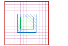
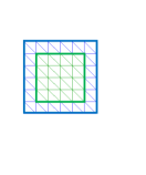
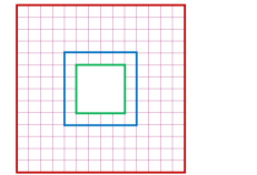
c)
Figure 1: Domain decomposition and mesh discretization
in . The mesh of is a combination of the
quadrilateral finite difference mesh presented
on c), and the finite element mesh presented on
b). Domains and overlap by
two layers of structured nodes such that they have common
boundaries shown by green and blue colors.
We now describe the DD method between two domains, and
, where the FEM is used for computation of the solution
in , and FDM is used in . Communication
between and is achieved letting
overlapping of both meshes across a two-element thick layer around
- see Figure 1. The common nodes of both
and domains belong to either of
the following boundaries (see Figure 1):
•
Nodes on the blue boundary - lie on the boundary of and are interior to ,
•
Nodes on the green boundary - lie on the inner boundary of
and are
interior to .
Then the main loop in time for the explicit hybrid FEM/FDM scheme, that solves
(2) associates with appropriate boundary conditions, at each time step is described in
Algorithm 1 below:
Algorithm 1 Domain decomposition process for hybrid FE/FD scheme
1: On the mesh , where FDM is
used, update the Finite Difference (FD) solution.
2: On the mesh , where FEM is used, update the
Finite Element (FE) solution.
3: Copy FE solution obtained at nodes (nodes on the green boundary
of Figure 1)
as a
boundary condition on the inner boundary for the FD solution in .
4: Copy FD solution obtained at nodes (nodes on the blue boundary
of Figure 1)
as a boundary condition for the FE solution on of .
5: Apply boundary condition at at the red boundary of .
By (3), at the overlapping nodes between and
. Thus, FEM and FDM schemes coincide on the
common, structured, overlapping layer. Hence, we avoid
instabilities at interfaces.
4 Derivation of computational schemes
In this section we construct, combined, finite element-finite
difference schemes to solve the model problem (6). To do this, first we present the finite
element scheme to solve
(6) in entire . This induces
the finite element scheme in . Then, we derive the finite difference scheme in , when the
domain decomposition FE/FD structure is applied to solve (6) in .
Remark
The computational schemes derived in this section are explicit and therefore, for their converegence, the CFL condition below (see ,e.g. [6, 7]) should be satisfied
(7)
Here is a mesh independent constant,
is the time step, and is the mesh size.
In the sequel, we denote the inner product of
by , and the corresponding norm by .
The scalar inner product in we denote by
, and the associated norm by .
Further, we let to be the boundary of , the inner boundary of and the outer boundary of .
4.1 Finite element discretization in
First we derive finite element scheme to solve the model problem (6) in whole
. Next, we discretize in two steps:
(i) the spatial discretization using
a partition of into elements , where
is a mesh function
defined as , representing the local diameter of elements.
We also denote by a partition of
the boundary into boundaries of the elements such that, at least one of the vertices of these elements belong to .
(ii) As for temporal discretization,
we let be a uniform partition of the time interval into
subintervals of length
As usual,
we also
assume a minimal angle condition on elements in .
To formulate the finite element method for (6) in ,
we introduce the finite element space for each component of the electric field defined by
where denote the set of piecewise-linear functions on .
Setting we define (resp. ) to be the
usual -interpolant of
(resp. ) in (6).
Also, because of the Dirichlet boundary data in
(6) we need to choose the test function space as
(8)
Then, recalling (4), and the fact that
the spatial semi-discrete problem in
reads:
Find such that
,
(9)
We note that
implies that
(10)
Recalling (8), vanishing test functions at the boundary yields
, and
the final weak formulation for the semi-discrete problem in is:
Find such that ,
(11)
For the, reflexive, inhomogeneous boundary condition, see the FE scheme for .
To get fully discrete scheme for
(6) we apply time discretization to (9) approximating , denoted
by , where we use the central difference scheme, for :
Rearranging terms in (13) we get the following scheme: Given the approximate initial data, and ,
find such that ,
(14)
4.2 Finite element discretization in
To solve the model problem (6) via the domain decomposition
FE/FD method, we use the split , see Figure 1.
Thus in we use FEM to solve the equation
(15)
Here, is the restriction of the solution obtained by the FDM in
to and therefore the test functions are
not vanishing at the boundary and hence the term corresponding to in (9) will be appearing in
the weak formulation.
To formulate the finite element method for (15) in , mimiking
(9),
we introduce the finite element space for each component of the electric field defined by
Setting we define
, , and to be the usual -interpolants of
, , and , respectively, in . Then, similar to the FE scheme for ,
we get the following finite element scheme for :
Given , , and , find
such that
(16)
A corresponding fully discrete problem in reads as follows:
Given , , , , and ; find such that
(17)
Remark
Note that, in (15), Dirichlet boundary condition can be
considered as well.
4.3 Fully discrete FE scheme for the electric field in
We expand the functions in
terms of the standard continuous piecewise linear functions
in space as
(18)
where denote unknown coefficients at and the spatial mesh point
. Then, substituting of (18) in
(14), and setting
,
we obtain the linear system of equations:
(19)
Note that, unlike (14), now the contributions at boundary of the element appear in
.
Here, are the block mass matrices in space, are the block stiffness matrices in space, denote the nodal values
of , and is a uniform time step.
Now we define the mapping from the reference element onto
such that and let be the piecewise
linear local basis function on such
that . Then, the explicit formulas
for the entries in system of equations (19), for each element , can be
written as:
(20)
where , and , denote
the , and , scalar products on and , respectively. Note that here
is only the part of the boundary of element that lies at .
To obtain fully explicit scheme we approximate with the lumped mass
matrix , (see [14, 18, 6] for the details corresponding to
the Maxwell’s system (2)).
Next, we multiply (20) by , and
get the following explicit, fully discrete method in :
(21)
4.4 Fully discrete scheme for the electric field in
As in the fully discrete FE scheme
(19) in ,
we obtain fully discrete FE scheme in
in the domain decomposition setting:
Expanding the functions of via the
continuous piecewise linear functions in space as in (18),
and then substituting them in (17), (with
, and
), we get the linear system of equations:
(22)
Here, is the block mass matrices in space, restricted to , otherwise the
same as in (19), are the block stiffness matrices in
space as in (19), is the assembled load
vector , denote the nodal values of ,
is the time step. All quantities are for .
Defining the mapping for the reference
element in the mesh generated in as
in the previous section, the formulas for entries of all matrices in the system
(22) are the same as those in (20), and the entries of load
vector are computed as
(23)
Again, approximating with the lumped mass matrix , we obtain the following fully explicit scheme:
(24)
4.5 Finite difference formulation
We recall now that from conditions (3) it follows that in
the function .
This means that in
for the model problem (2) the forward problem will be
(25)
(26)
(27)
(28)
Using standard finite difference discretization of the
equation (25) in we obtain the following explicit
scheme for the solution of the forward problem:
(29)
In the, system of, equations above,
is the solution at the time iteration at the
discrete point ,
is the time step, and is the discrete Laplacian.
Note that, in (29), the Dirichlet boundary consitions can be
considered as well.
5 Stability
In this section we derive stability estimates for the semi-discrete approximations. For stability in
these estimates are extensions of
the stability approach derived for the continuous problem
in [4]. As for the stability in we get slightly different norms involving
contributions corresponding to the
reflexive boundary: .
We use discrete version of a triple norm
induced by the weak variational formulation of
(6), where we use the relation
(10) (which is not necessary in the continuous case where
, however, in general ):
Find such that
(30)
Remark
In general, in non-divergent free case, the bilinear form induced by (30) is not coercive. Further
-conforming finite element may result in spurious solutions. A remedy is through
modifying the equation by adding a gauge constrain of Coulomb-type, see, e.g. [21] and [23].
This is supplied by the ”zero”-term: , in (6), which we
add in the continuous variational formulation in (9). This, however, is not necessarily true
in the discrete forms, e.g. in (16), where most likely
Taking in (30), (we used the boundary condition on
), yields
(31)
which, due to the fact that is independent of ,
can be rewritten as
Let be a bounded domain with piecewise linear boundary
. Then, the equation (6) has a unique solution . Further
Let and
, then there is a constant such that, , the following
stability estimate holds true
(33)
Proof.
The estimate (33) is proved in [4], Theorem 4.1 by
setting and .
Integrating (33) over the time interval we get the desired result.
We omit the details.
∎
Below we translate this stability to the semi-discrete problem.
5.1 Stability estimate for the semi-discrete problem in
The stability for the semi-discrete problem in is basically as in the continuous case above
where all :s are
replaced by with some relevant assumptions in the discrete data, viz.
Lemma
Assume that the interpolants of the data and : and
satisfy the regularity conditions and
,
then for each
(34)
where
(35)
5.2 Stability of the semi-discrete problem in
The stability of the semi-discrete problem in ,
relying on the variational formulation
(16), and due to the appearance of the data function , is slightly
different from (34). We rewrite (16), in view of
(10), and with as:
Given , , and , find
such that
(36)
To deal with the -term we rewrite
(36) in its original form as (9) for and with :
(37)
Once again, in view of Theorem 4.1 in [4], as in the case of stability in , we end up with
the following time derivative form in norms:
(38)
Hence, integrating (38) over the time interval , we get ,
(39)
Remark
We don’t have electric conductivity: -term on the right hand side here.
With the presence of as in (6), the associated assumptions are
in and for
. As fot the boundary terms, we may either use trace theorem and
hide the -terms in
in (39), or redefine a modified version of
adding terms corresponding to contributions
from the boundary boundary.
For the sake of generality we keep the two integrals as is and assume,
for the boundary data,
.
Summing up we have the following stability estimate for the semi-discrete
problem in :
Lemma
Under the following regularity assumptions on the interpolants for initial conditions:
,
,
, and with both boundary data:
, and , we have,
for all , the following
stability estimate for the semi-discrete problem
(40)
Corollary
We could write the right hand side in (36) as
.
Then letting , the inequality
(40) can be rewritten as
(41)
Thus by the definition of the triple norm and using Cauchy-Schwarz, Poincare and Grönwall’s inequalities
(42)
In a simlar way one may derive estimates of the gradient ()-terms in the triple norm using
the trace theorem, viz.
(43)
Now since both likewise
contributions from the right hand side
terms can be hidden in
corresponding terms of the triple norm, thus ending up with function and gradient terms estimates
with bounds depending on given parameters and functions
.
We omit the details.
6 Error estimates: Semi-Discrete (SD) problems
In what follows, and for future use in our model problems,
we shall assume that on ,
which has the common value on .
Let now , with
or , be an spatial interpolant of the
exact electric field and set
(44)
Then, assuming certain regularity of the data set, and with
,
and with the spectral order , we can prove error estimates of the form
(45)
In this section, and to make a direct error estimate approach, without relying on the stability norm
defined in [4], we use the equivialent norm , slightly different
form the norm in (33), (see the term ), and
directly obtained from the equation (11):
(46)
Further, by the coercivity modification, see e.g. [21], there is a constant such that
(47)
Finally
(48)
likewise
(49)
Remark
The original problem, with the presence of the electric conductivity terrm :
() on the right hand side, would behave as of parabolic type,
(actually, quasi-parabolic, due to the presence of -term).
Then in
(45), and for , . But in our current consideration
, and the problem is viewed as a system of wave equations
(componenmtwise for E:s) and hence hyperbolic. On the other hand finite elements for
the scalar (non-system) hyperbolic problems has been considered in various studies by several
authors, showing that
the best convergence one can hope is obtained using, e.g. discontinuous
Galerkin (see [20]), which yields
(50)
instead of
(45) and with , whereas the finite difference approach for the same, hyperbolic type, problem
is more accurate and satisfies (45).
Below we use the very similar argument to
derive (45) for the spatial domains and .
6.1 Error estimates: SD problem in
Theorem
For and
continuous piecewise polynomial approximation,
assuming
then there is a constant such that
(51)
Proof.
We start with the straightforward estimate for in (44), using
interpolation error:
(52)
Note that if , then the continuous interpolation, (52)
is improved, and
However, such improvement can not survive, e.g. in approximating with discontinuous interpolation
where jump terms are introduced in the outward normal directions to elements,
and
Hence, we have the following estimate for the interpolation error:
(53)
where the last two inequalities are just the consequences of the interpolation error and regularity of the exact solution, respectively. So that we can deduce that the interpolation error is:
(54)
To proceed further we assume continuous variational formulation, i.e.
the continuous version of (11):
Hence we can write for
(55)
and hence, in a time interval we have
(56)
where
(57)
We estimate each for , separately. As for , partial integration, with zero boundary condition, yields
(58)
Direct estimates for , (with some formal manipulations), and -terms give
(59)
(60)
(61)
Thus by a kick back argument
all -norms on the right hand side,
can be hidden in the corresponding terms in leading to a
estimate for :
With the same assumption as in the theorem 6.1 above we have the convergence rate of the time derivative for the error:
(63)
Proof.
Evidently the interpolation estimates in the proof of theorem 6.1 also yield for , and
(64)
Note that we have no time discretization yet. The remaining step is to show that
(65)
The same proceedure with and replaced by and , respectively, yields
(66)
and hence
(67)
where
(68)
Mimiking the above procedure we estimate -terms for , viz.
(69)
where, with the continuous in time, the spatial discrete errors for and
are assumed to be zero for all .
(70)
(71)
(72)
Note that due to the vanishing boundary condition, the contribution from the boundary is not present.
This however can be inserted by considering a modified triple norm including, e.g., reflecting
boundaries as in the case of below.
Hence, once again, a kick-back argument, with all and weighted-norms on the left hand side
are hidden in the corresponding terms in giving the
estimate (65) for ,
which, combined with
(64), gives the desired result.
∎
6.2 Error estimates: SD problem in
The estimates here are mostly the same as those of ther previous subsection. However,
here we have a reflexive boundary condition on . Hence, the
estimates contain an extra contribution from the boundary
( in the previous subsection, we have only considered
the zero boundary condition for the whole ). Here, we include the procedure containg
boudarry trerm estimates, which can be mimiked in the case of the refexive boundary condition in whole .
Theorem
Let and consider
the continuous piecewise polynomial approximation for the solution of the problem
(15). Furthermore, assume that ,
,
and
.
Then there is a constant such that
(73)
Proof.
Following the same procedure as the error estimates in , and letting now
(74)
we need to estimate a triple norm of the form
(75)
Assuming that, at the boundary , is as regular as ,
the linear interpolation error reads:
(76)
Then following the same procedure as above we have for both (16)
and its continuous version, and with and corresponding to
and , respectively, we have
(77)
with the associated data.
Hence we can write
(78)
In the triple norm form this yields
(79)
Now using the same procedure as in the proof of the previous theorem
(with and replaced by and ) to bound all the involved norms
and hiding both -terms on the right, inside
, on the left hand side,
together with estimates (76)
for , and further assuming corresponding estimates for
, we obtain (omitting some details)
that
(80)
Now
(76) and (80) together with the corresponding
estimates for , give the desired result and completes the proof.
∎
Algorithm 2 Domain decomposition algorithm for solution of Maxwell’s equations (2). At every time step are performed the following operations:
1: Compute in using the explicit
finite difference scheme (29) with known , and
-values.
2: Compute in by using the finite
element scheme (22) with known .
3: For the finite
difference method in , use the values of the function at nodes
(green boundary of Figure 1) , which are computed using the finite element
scheme (24), as a boundary condition at the inner boundary of .
4: Apply appropriate boundary condition at the outer boundary of .
5: For the finite element
method in , use the values of the functions at
nodes (blue boundary of the Figure 1 ),
which are computed using the finite difference
scheme (29) as a boundary condition.
6: Apply swap of the solutions for the computed function
to be able to perform the algorithm on a new time level .
7 Numerical examples
In this section we present numerical examples justifying theoretical results of the previous two sections.
For convergence tests the domain decomposition algorithm (see Algorithm 2),
implemented in the software package WavES [31], was used.
We note that because of
using explicit FE and FD schemes in and , correspondingly, we need to choose time step according to the CFL stability condition (7) derived in [6] so that
the whole hybrid scheme remains stable.
Numerical tests are performed in time interval and in the spatial dimensionless
computational domain
(81)
which is split into the finite element domain
(82)
and the finite difference domain , thus
, see Figure 1.
The model problem in all our tests that is stated for the electric field is as follows:
(83)
We have the functions
(84)
as the exact solution of the model problem
(83) with the source data which corresponds to
this exact solution.
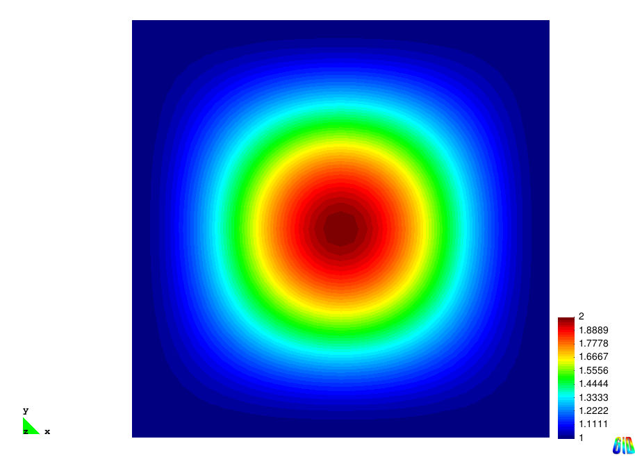
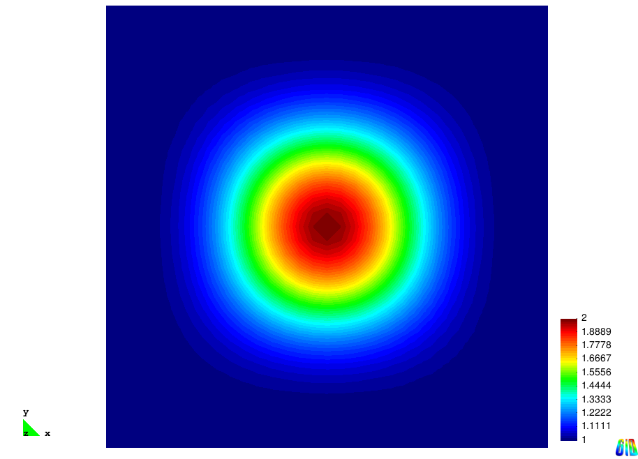
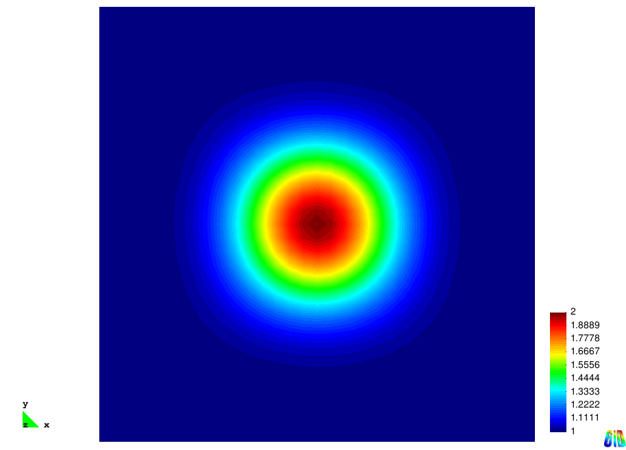
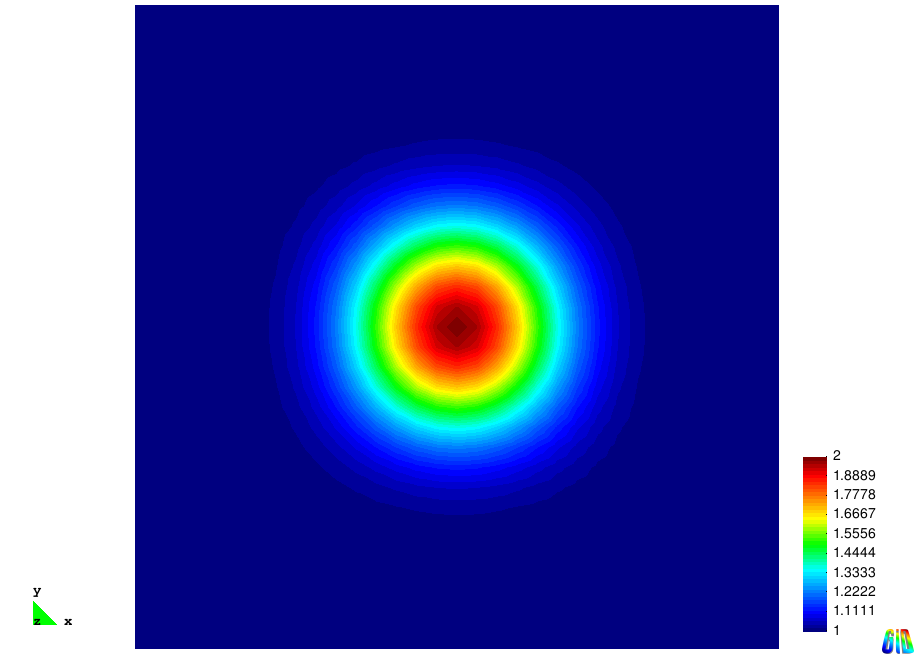
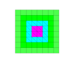
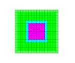
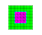
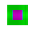
We choose in our numerical examples, see Figure 2, for these functions
in the domain . We note that the exact solution (84) satisfies the divergence free condition for
defined by (85), the homogeneous
initial conditions, as well as the homogeneous Dirichlet conditions for all times.
Figure 2: Function in the domain for different values of in (85).
The computational domain was discretized
into triangular elements with mesh sizes , and the mesh in
was decomposed into squares of the same
mesh sizes as described in Section 3, see Figure
1. The time step was chosen corresponding to the
stability criterion (7) as for . Convergence results of the proposed finite
element scheme computed in
and norms are presented in Tables 2 - 4 for in (85).
Relative norms in these tables were computed as
(86)
and are the exact and computed FE solutions in , respectively, and .
Logarithmic convergence rates in these tables are computed, viz.
(87)
where are relative norms computed via (86) on the mesh with the mesh
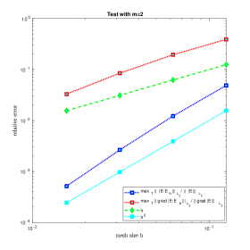
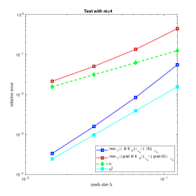
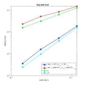
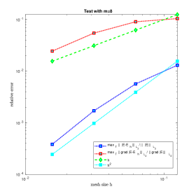
size and , respectively. Figure 3 shows
convergence of the relative and norms computed via
(86) and compared with exact behavior of and .
m=2
m= 4
m=6
m=8
Figure 3: Convergence of the relative and norms computed via (86).
Table 1: Relative errors and in the - and -norms, respectively, for
mesh sizes , for in (85).
Table 2: Relative errors and in the -norm and in the -norm, respectively, for
mesh sizes , for in (85).
Table 3: Relative errors and in the -norm and in the -norm, respectively, for
mesh sizes , for in (85).
Table 4: Relative errors and in the -norm and in the -norm, respectively,
for
mesh sizes , for in (85).
Computational meshes in the domain decomposition of
Exact solution , in
Computed domain decomposition solution , in
Computed finite difference solution , in the domain decomposition algorithm in
Figure 4: Computed vs. exact solution at the time for different meshes taking in (85). Algorithm 2 was used in the domain decomposition method. Common elements in and on different meshes are presented on the top figures and are outlined by light blue color. We observe smooth hybrid solution across FE/FD boundaries.
Computed hybrid FE/FD versus exact solutions with in (85)
at the time are presented in Figures 4, where
is computed
using the domain decomposition algorithm (Algorithm 2)
for different meshes with sizes . The top figures
of Figure 4
present hybrid FE/FD meshes which were used for computations;
common hybrid FE/FD solution in is presented in the middle figures, and bottom figures
show only FD solution as the part of the common hybrid solution in
. Interpreting these
figures we observe smooth behavior of the hybrid solution across
finite element/finite difference boundary, as was predicted in theory.
Furthermore, through these figures, as well as tables and Figure 3, we
observe that with increasing in , the
computational errors approach the second order convergence in
- and first order in -norm for
. Therefore, we can conclude that the finite element
scheme in the hybrid FE/FD method; considered in , behaves like a first order
method in -norm and a second order method in the -norm.
These results are all in good agreement with the analytic estimates
derived in Sections 5-6, as well as with results presented for
finite element method in [6, 7] for the whole .
Conclusion
In this paper we present stability and convergence analysis
for the domain decomposition
FE/FD method for time-dependent
Maxwell’s equations developed in [3, 4].
The convergence is optimal due to the assumed maximal available regularity of the exact solution
in a Sobolev space.
The analysis are performed for the semi-discrete (spatial discretization) problem for, the constructed, finite
element schemes in two different
settings: in and . The temporal discretization algorithms are constructed using
the CFL condition (7) derived in [6].
We have
implemented several numerical
examples that validate the robustness of the theoretical studies.
In a forthcoming, complementary, study we plan to extend the results in here to a problem with the
presence of electrical conductivity term which renders the equation to an parabolic-hyperbolic one.
Acknowledgments
The research of both authors
is supported by the Swedish Research Council grant VR 2018-03661. The first
author acknowledges the support of the VR grant DREAM.
References
[1]
[2] L. Beilina, Application of the finite element method in a
quantitative imaging technique, J. Comput. Methods
Sci. Eng., IOS Press, 16(4), 755-771, 2016. DOI 10.3233/JCM-160689.
[3] L. Beilina, M. Grote, Adaptive Hybrid Finite Element/Difference method for Maxwell’s equations,
TWMS Journal of Pure and Applied Mathematics, 1 (2) s. 176-197, 2010.
[4] L. Beilina, Energy estimates and numerical
verification of the stabilized Domain Decomposition Finite
Element/Finite Difference approach for time-dependent Maxwell’s
system, Cent. Eur. J. Math., 11 (2013), 702-733 DOI:
10.2478/s11533-013-0202-3.
[5] L. Beilina, Domain decomposition finite element/finite difference method for the conductivity reconstruction in a hyperbolic equation, Communications in Nonlinear Science and Numerical Simulation, Elsevier, 2016, doi:10.1016/j.cnsns.2016.01.016
[6] L. Beilina, V. Ruas, Convergence of Explicit P1 Finite-Element Solutions to Maxwell’s Equations, Springer Proceedings in Mathematics and Statistics, vol 328. Springer, Cham (2020)
[7] L. Beilina, V. Ruas, An explicit P1 finite element scheme for Maxwell’s equations with constant permittivity in a boundary neighborhood, arXiv:1808.10720v4
[8] L. Beilina, N. T. Thánh, M. Klibanov, and
J. B. Malmberg, Reconstruction of shapes and refractive indices from
blind backscattering experimental data using the adaptivity, Inverse
Problems, 30 (2014), 105007.
[9] L. Beilina, N. T. Thánh, M.V. Klibanov and
J. B. Malmberg, Globally convergent and adaptive finite element
methods in imaging of buried objects from experimental
backscattering radar measurements, Journal of Computational
and Applied Mathematics, Elsevier, DOI: 10.1016/j.cam.2014.11.055,
2015.
[10] J. Bondestam Malmberg, L. Beilina, An Adaptive
Finite Element Method in Quantitative Reconstruction of Small
Inclusions from Limited Observations, Appl. Math. Inf. Sci., 12(1), 1-19, 2018.
[11] G. C. Cohen, Higher Order Numerical Methods for
Transient Wave Equations, Springer-Verlag, Berlin, 2002.
[12] T. Chan and T. Mathew, Domain decomposition algorithms,
In A. Iserles, editor, Acta Numerica, 3, Cambridge University
Press, Cambridge, 1994.
[13] F. Edelvik, U. Andersson and G. Ledfelt, (2000), Explicit hybrid time domain solver
for the Maxwell equations in 3D, AP2000 Millennium Conference on Antennas & Propagation, Davos.
[14] A. Elmkies and P. Joly, Finite elements and mass lumping for Maxwell’s equations: the 2D case. Numerical Analysis, C. R. Acad.Sci.Paris, 324, pp. 1287–1293, 1997.
[15] B. Jiang, The Least-Squares Finite Element Method. Theory and Applications in Computational Fluid Dynamics and Electromagnetics, Springer-Verlag, Heidelberg, 1998.
[16] B. Jiang, J. Wu and L. A. Povinelli, The origin of spurious solutions in computational electromagnetics, Journal of Computational Physics, 125, pp.104–123, 1996.
[17] J. Jin, The finite element method in electromagnetics, Wiley, 1993.
[18] P. Joly, Variational methods for time-dependent
wave propagation problems, Lecture Notes in Computational Science
and Engineering, Springer, 2003.
[19] G. Chavent, Nonlinear Least Squares for Inverse Problems. Theoretical Foundations and Step-by-
Step Guide for Applications, Springer, New York, 2009.
[20]
C. Johnson and J. Pitkäranta, Analysis of a the discontinuous Galerkin method for linear hyperbolic equations,
Math. Comp., 46 (173), pp.1-26, 1986.
[21] P. B. Monk, Finite Element methods for Maxwell’s equations, Oxford University Press, 2003.
[22] P. B. Monk and A. K. Parrott, A dispersion
analysis of finite element methods for Maxwell’s equations, SIAM
J.Sci.Comput., 15, pp.916–937, 1994.
[23] C. D. Munz, P. Omnes, R. Schneider, E. Sonnendrucker
and U. Voss, Divergence correction techniques for Maxwell
Solvers based on a hyperbolic model, Journal of Computational Physics, 161,
pp.484–511, 2000.
[24] J.-C. Nédélec, Mixed finite elements in R3,
Numerische Mathematik, 35 (1980), 315-341.
[25] K. D. Paulsen, D. R. Lynch, Elimination of vector parasites in Finite Element Maxwell solutions, IEEE Transactions on Microwave Theory Technologies, 39, 395 –404, 1991.
[26] T. Rylander and A. Bondeson, (2000), Stable FEM-FDTD hybrid method for Maxwell’s equations, J. Comput.Phys.Comm., 125.
[27] T. Rylander and A. Bondeson, (2002), Stability of Explicit-Implicit Hybrid Time-Stepping Schemes for Maxwell’s Equations, J. Comput.Phys.
[28] N. T. Thánh, L. Beilina, M. V. Klibanov, and M. A. Fiddy, Reconstruction of the refractive
index from experimental backscattering data using a globally convergent inverse method, SIAMJ. Sci. Comput., 36 (2014), pp. B273-B293.
[29] N. T. Thánh, L. Beilina, M. V. Klibanov,
M. A. Fiddy, Imaging of Buried Objects from Experimental
Backscattering Time-Dependent Measurements using a Globally
Convergent Inverse Algorithm, SIAM Journal on Imaging
Sciences, 8(1), 757-786, 2015.
[30] A. Toselli and B. Widlund, Domain Decomposition
Methods, Springer, Berlin, 2005.
[31] Software package WavES at http://www.waves24.com/