Heron triangles with two rational medians and Somos-5 sequences

Abstract

Triangles with integer length sides and integer area are known as Heron triangles. Taking rescaling freedom into account, one can apply the same name when all sides and the area are rational numbers. A perfect triangle is a Heron triangle with all three medians being rational, and it is a longstanding conjecture that no such triangle exists. However, Buchholz and Rathbun showed that there are infinitely many Heron triangles with two rational medians, an infinite subset of which are associated with rational points on an elliptic curve $E({\mathbb{Q}})$ with Mordell-Weil group ${\mathbb{Z}}\times{\mathbb{Z}}/2{\mathbb{Z}}$, and they observed a connection with a pair of Somos-5 sequences. Here we make the latter connection more precise by providing explicit formulae for the integer side lengths, the two rational medians, and the area in this infinite family of Heron triangles. The proof uses a combined approach to Somos-5 sequences and associated Quispel-Roberts-Thompson (QRT) maps in the plane, from several different viewpoints: complex analysis, real dynamics, and reduction modulo a prime.

1 Introduction

The formula

$$\Delta=\sqrt{s(s-a)(s-b)(s-c)}$$ (1.1)

for the area of a triangle with sides $(a,b,c)$, where

$$s=\frac{a+b+c}{2}$$

is the semiperimeter, is attributed to Heron of Alexandria. If $(a,b,c)$ is a triple of positive integers and the area $\Delta$ is also an integer, then this is called a Heron triangle. More generally, due to rescaling freedom, we say that a triangle is Heron whenever the side lengths and the area are all rational numbers. A method for enumerating Heron triangles was given by Schubert in [48], but a parametric formula equivalent to

$$a=\frac{p^{2}+r^{2}}{p},\qquad b=\frac{q^{2}+r^{2}}{q},\qquad c=\pm\frac{(r^{2}-pq)(p+q)}{pq},$$ (1.2)

for $p,q,r\in{\mathbb{Q}}$ and area $\Delta=rc\in{\mathbb{Q}}$ was already known to Brahmagupta in the 7th century A.D. [10]. Any Pythagorean triple gives a right-angled Heron triangle, while the triangle with integer side lengths $(5,5,6)$ and area $12$ arising from the choice $p=q=1,r=2$ in Brahmagupta’s formula is the simplest isosceles Heron triangle (in the sense of having the smallest value of $a+b+c$), and the simplest example of a Heron triangle that is neither right-angled nor isosceles has side lengths $(15,13,14)$ and area $84$, being obtained by taking $p=3,q=4,r=6$ in the same formula. There are numerous Diophantine problems concerning Heron triangles, many of which are related to the theory of elliptic curves [13, 23, 30, 40].

It is an old problem to answer the question as to whether there exists a perfect triangle: one with integer sides, medians, and area; or equivalently, is there a Heron triangle with three rational medians? The expectation is that there is no such triangle, but to prove it seems very difficult, and it is remarked in [26] that despite incorrect “proofs” in the literature, the problem remains open. One of the first incorrect arguments is implicit in Schubert’s work [48], where he claimed to present a complete parametrization of Heron triangles with one of the medians being rational, and used this to argue that Heron triangles with two rational medians are impossible. However, his proposed parametrization was incomplete, and Schubert’s oversight was pointed out by Dickson [10] and in the PhD thesis of Buchholz [6], who initially found the case $(73,51,26)$ with area $420$ and two rational medians, of lengths $\frac{35}{2}$ and $\frac{97}{2}$ respectively, as well as a small number of other examples - see Table 1, in which each triangle is represented (up to scale) by an integer triple with $\gcd(a,b,c)=1$.

Figure 1: Triangle with one labelled median

Henceforth we denote the medians that bisect sides $a,b,c$ by $k,\ell,m$, respectively, so that

$$k^{2}=\frac{1}{4}(2b^{2}+2c^{2}-a^{2}),\quad\ell^{2}=\frac{1}{4}(2c^{2}+2a^{2}-b^{2}),\quad m^{2}=\frac{1}{4}(2a^{2}+2b^{2}-c^{2}),$$ (1.3)

and label the angles adjacent to the median $k$ as in Fig.1. Then the area of the triangle satisfies $\Delta=bk\sin{\alpha}=ck\sin{\beta}=\frac{1}{2}ak\sin{\gamma},$ and, following [48], it is helpful to consider the half-angle cotangents

$$M=\mathrm{cot}({\alpha}/2),\quad P=\mathrm{cot}({\beta}/2),\quad X=\mathrm{cot}({\gamma}/2),$$ (1.4)

which we will refer to as the Schubert parameters, using the same nomenclature and notation as in [7]. Up to rescaling, these three parameters completely determine the triangle; clearly they are not independent, but as shown by Schubert they satisfy the equation

$$M-\frac{1}{M}=P-\frac{1}{P}+2\left(X-\frac{1}{X}\right).$$ (1.5)

Upon rewriting the latter as $2MP(X^{2}-1)+MX(P^{2}-1)-PX(M^{2}-1)=0$, we see that this defines an affine quartic surface in three dimensions, which we call the Schubert surface. The Schubert parameters are given in terms of the area, side lengths and the median $k$ by the formulae

$$M=\frac{4\Delta}{4bk+a^{2}-3b^{2}-c^{2}},\quad P=\frac{4\Delta}{4ck+a^{2}-b^{2}-3c^{2}},\quad X=\frac{4\Delta}{2ak-b^{2}+c^{2}},$$ (1.6)

which follow from the half-angle identity $\mathrm{cot}({\alpha}/2)=\sin{\alpha}/(1-\cos{\alpha})$ and the cosine rule, while the ratios of side lengths are given in terms of the Schubert parameters by

$$\frac{a}{c}=\frac{2(X+X^{-1})}{P+P^{-1}},\qquad\frac{b}{c}=\frac{M+M^{-1}}{P+P^{-1}}.$$ (1.7)

Table 1: The smallest Heron triangles with two rational medians.

$n$	$a$	$b$	$c$	$k$	$\ell$	$\Delta$
1	73	51	26	${35}/{2}$	${97}/{2}$	420
2	626	875	291	572	${433}/{2}$	55440
*	1241	4368	3673	${7975}/{2}$	1657	2042040
**	14384	14791	11257	11001	21177/2	75698280
3	28779	13816	15155	3589/2	21937	23931600
4	1823675	185629	1930456	2048523/2	3751059/2	142334216640
***	2288232	1976471	2025361	1641725	3843143/2	1877686881840
****	22816608	20565641	19227017	16314487	36845705/2	185643608470320
5	2442655864	2396426547	46263061	1175099279	2488886435/2	2137147184560080

In view of the formulae (1.6), for a Heron triangle with rational median $k$ the corresponding Schubert parameters are rational, and conversely, if $(M,P,X)\in{\mathbb{Q}}^{3}$ is a rational point on the Schubert surface (1.5), then the triangle is Heron with (at least) one rational median. Strictly speaking, we require positive rational solutions, since the half-angle cotangents must be positive, but the surface (1.5) admits the obvious involutions $M\to-M^{-1}$, $P\to-P^{-1}$, $X\to-X^{-1}$, as well as $(M,P,X)\to(M^{-1},P^{-1},X^{-1})$, so if one of the coordinates is negative it can be replaced by minus its reciprocal, while all three coordinates can simultaneously be replaced by their reciprocals, and we shall exploit this freedom in what follows. The inherent subtlety in the problem of characterizing Heron triangles with one rational median, to which Schubert gave an incomplete solution, can be seen from the fact that the Schubert surface admits three different elliptic fibrations, obtained by fixing the value of any one of the parameters. For instance, setting $M=M_{0}\in{\mathbb{P}}^{1}({\mathbb{Q}})$ gives the cubic curve $2P(X^{2}-1)+X(P^{2}-1)+CPX=0$, where the constant $C=1/M_{0}-M_{0}$; so for generic values of $C$ the fibre is an elliptic curve, with j-invariant $(C^{4}+40C^{2}+208)^{3}/\big{(}16(C^{4}+40C^{2}+144)\big{)}$, and each (finite) element of the group of rational points on the curve corresponds to a Heron triangle with one rational median.

For a Heron triangle with two rational medians $k,\ell$, there are two associated rational points on the Schubert surface, namely the point $(M_{a},P_{a},X_{a})$ associated with the median $k$ bisecting side $a$, as given by the formulae (1.6), and the point $(M_{b},P_{b},X_{b})$ associated with the median $\ell$ bisecting side $b$, given by the same formulae but replacing $a\to b$, $b\to c$, $c\to a$ and $k\to\ell$. As well as satisfying the equation (1.5), these two sets of Schubert parameters must be related by the compatibility conditions

$$\frac{2(X_{a}+X_{a}^{-1})}{P_{a}+P_{a}^{-1}}=\frac{P_{b}+P_{b}^{-1}}{M_{b}+M_{b}^{-1}},\qquad\frac{M_{a}+M_{a}^{-1}}{P_{a}+P_{a}^{-1}}=\frac{2(X_{b}+X_{b}^{-1})}{M_{b}+M_{b}^{-1}},$$ (1.8)

corresponding to the ratios of the side lengths as in (1.7). Thus the problem of finding a Heron triangle with two rational medians is equivalent to finding a pair of positive rational points on the Schubert surface (1.5), subject to the pair of constraints (1.8). The angles ${\alpha},{\beta}$ as in Fig.1 must also satisfy ${\alpha}+{\beta}<\pi$, so this imposes the additional requirements

$$\mathrm{arccot}(M_{a})+\mathrm{arccot}(P_{a})<\frac{\pi}{2},\qquad\mathrm{arccot}(M_{b})+\mathrm{arccot}(P_{b})<\frac{\pi}{2},$$ (1.9)

but once a pair of compatible positive triples has been found, these requirements can always be satisfied by applying $(M_{a},P_{a},X_{a})\to(M_{a}^{-1},P_{a}^{-1},X_{a}^{-1})$ and/or $(M_{b},P_{b},X_{b})\to(M_{b}^{-1},P_{b}^{-1},X_{b}^{-1})$ if necessary, since these transformations leave the constraints (1.8) invariant.

There is another approach to the problem, based on the formulae

$$\begin{array}[]{rcl}a&=&\uptau\,(-2\theta^{2}\phi-\theta\phi^{2}+2\theta\phi-\phi^{2}+\theta+1),\\ b&=&\uptau\,(\theta^{2}\phi+2\theta\phi^{2}-\theta^{2}+2\theta\phi-\phi+1),\\ c&=&\uptau\,(\theta^{2}\phi-\theta\phi^{2}+\theta^{2}+2\theta\phi+\phi^{2}+\theta-\phi),\end{array}$$ (1.10)

found by Buchholz [6], which provide a rational parametrization of triangles with two rational medians $k,\ell$, where $\theta,\phi$ are rational numbers (constrained suitably to ensure positivity), and the parameter $\uptau\in{\mathbb{Q}}$ allows for the arbitrary choice of scale. Conversely, $\theta,\phi\in{\mathbb{Q}}$ can be written as functions of the (ratios of) side lengths, given by

$$\theta=\frac{c-a\pm 2\ell}{2s},\qquad\phi=\frac{b-c\pm 2k}{2s},$$ (1.11)

with $s=\frac{1}{2}(a+b+c)$ being the semiperimeter, as before.

Hence an efficient method to search for Heron triangles with two rational medians is to run through the rational parameters $\theta,\phi$, ordered by height, and check whether the corresponding value of $\Delta$ is a rational number. More precisely, given $\theta=R/S\in{\mathbb{Q}}$ written as a fraction in lowest terms, its naive height is $H(\theta)=\max(|R|,|S|)$, and pairs $(\theta,\phi)\in{\mathbb{Q}}^{2}$ can be enumerated in order of increasing height $\tilde{H}=\max\big{(}H(\theta),H(\phi)\big{)}$, so fixing the scale $\uptau=1$ in (1.10), the side lengths $(a,b,c)$ of triangles with two rational medians can be calculated from this parametrization for each pair of parameters with $\tilde{H}=1,2,3,\ldots$ and then it can be checked from Heron’s formula (1.1) whether $s(s-a)(s-b)(s-c)$ is a perfect square, corresponding to the area being rational. (This method leads to duplicate triangles related to one another by different values of the scaling $\uptau$, but still seems more efficient than finding Heron triangles with one rational median and then checking whether a second median is rational.)

The latter method was implemented by Buchholz and Rathbun, initially working independently (an independent search was also carried out by Kemnitz), yielding the first six rows in Table 1. In [7] they observed remarkable properties of certain triangles in the latter table, with respect to their Schubert parameters, which are shown in Table 2: for the rows labelled by an integer $n=1,2,3,\ldots$, the factorizations are related, and in particular the parameter $M_{b}$ in row $n$ is minus the reciprocal of the parameter $P_{a}$ in row $n+1$ (see Table 3 for details of the factorizations). The triangles labelled by asterisks do not seem to fit into any obvious pattern, but their observations on the other triangles (corresponding to $n=1,\ldots,5$ in Tables 1 & 2) led them to suggest that these examples should extend to an infinite family of triangles labelled by a positive integer $n$, with a conjectured factorization of the Schubert parameters as

$$M_{a}=-\frac{S_{n+1}S_{n+2}^{2}T_{n}}{S_{n}T_{n+1}T_{n+2}^{2}},\quad P_{a}=-\frac{S_{n+1}S_{n+2}T_{n+1}T_{n+2}}{S_{n}S_{n+3}T_{n}T_{n+3}},\quad X_{a}=2^{(-1)^{n+1}}\frac{S_{n}S_{n+2}^{2}T_{n+3}}{S_{n+3}T_{n}T_{n+2}^{2}},$$ (1.12)

$$M_{b}=\frac{S_{n+1}S_{n+4}T_{n+1}T_{n+4}}{S_{n+2}S_{n+3}T_{n+2}T_{n+3}},\quad P_{b}=-\frac{S_{n+2}^{2}S_{n+3}T_{n+4}}{S_{n+4}T_{n+2}^{2}T_{n+3}},\quad X_{b}=2^{(-1)^{n}}\frac{S_{n+1}T_{n+2}^{2}T_{n+4}}{S_{n+2}^{2}S_{n+4}T_{n+1}},$$ (1.13)

where $(S_{n})$ and $(T_{n})$ are integer sequences given by

$$(S_{n}):\quad 1,1,1,2,3,5,11,37,83,274,\ldots,$$ (1.14)

and

$$(T_{n}):\quad 0,1,-1,1,1,-7,8,-1,-57,391,\ldots,$$ (1.15)

(the terms above are listed starting from the index $n=0$). These are Somos sequences, of the kind introduced in [50]. More specifically, they are both Somos-5 sequences: $(S_{n})$ is generated by the fifth order quadratic recurrence

$$S_{n+5}S_{n}=S_{n+4}S_{n+1}+S_{n+3}S_{n+2}$$ (1.16)

(see [43]); the sequence is usually generated starting from five initial 1s, but here we have indexed it so that it extends symmetrically to negative $n$, with $S_{-n}=S_{n}$. As we shall see, the sequence $(T_{n})$ is closely related to $(S_{n})$: it is generated by the same fifth order recurrence (1.16), and extends backwards in an antisymmetric fashion, so that $T_{-n}=-T_{n}$; it is also a divisibility sequence, having the property that $T_{n}|T_{m}$ whenever $n|m$. (It is almost an elliptic divisibility sequence in the sense of [55], but the terms with even/odd index satisfy different relations of order four.) Henceforth we shall refer to the sequence of triangles corresponding to the pairs of Schubert parameters (1.12) and (1.13) as the main sequence.

Table 2: Schubert parameters (with signs) for the smallest Heron triangles with two rational medians.

$n$	$M_{a}$	$P_{a}$	$X_{a}$	$M_{b}$	$P_{b}$	$X_{b}$
0	0	$\infty$	$\infty$	-3/2	-2/3	2/3
1	4	2/3	8/3	35/6	84/5	7/40
2	18	-6/35	63/10	-176/105	360/77	32/99
*	728/51	17	48/91	231/260	2431/420	17/55
**	1395/476	620/153	63/85	357/95	4845/1736	1767/1360
3	-75/98	105/176	800/539	111/3080	275/14504	-147/1850
4	605/1344	-3080/111	-363/4736	-165585/3256	-255189/5312	36480/70301
***	7144/2277	79101/24472	7238/7429	394128/101365	49742 /11155	24035/27936
****	1035096/312455	1542840/505571	770431/717145	770431/218064	505571/117691	337421/412896
5	105413/40	3256/165585	780330/581	9427792/175047	44428157/15618	4301/6001696

Table 3: Prime factors of the first few Schubert parameters in the main sequence.

$n$	$M_{a}$	$P_{a}$	$X_{a}$	$M_{b}$	$P_{b}$	$X_{b}$
0	0	$\infty$	$\infty$	$-\tfrac{3}{2}$	$-\tfrac{2}{3}$	$\tfrac{2}{3}$
1	$2^{2}$	$\tfrac{2}{3}$	$\tfrac{2^{3}}{3}$	$\tfrac{5\cdot 7}{2\cdot 3}$	$\tfrac{2^{2}\cdot 3\cdot 7}{5}$	$\tfrac{7}{2^{3}\cdot 5}$
2	$2\cdot 3^{2}$	$-\tfrac{2\cdot 3}{5\cdot 7}$	$\tfrac{3^{2}\cdot 7}{2\cdot 5}$	$-\tfrac{2^{4}\cdot 11}{3\cdot 5\cdot 7}$	$\tfrac{2^{3}\cdot 3^{2}\cdot 5}{7\cdot 11}$	$\tfrac{2^{5}}{3^{2}\cdot 11}$
3	$-\tfrac{3\cdot 5^{2}}{2\cdot 7^{2}}$	$\tfrac{3\cdot 5\cdot 7}{2^{4}\cdot 11}$	$\tfrac{2^{5}\cdot 5^{2}}{7^{2}\cdot 11}$	$\tfrac{3\cdot 37}{2^{3}\cdot 5\cdot 7\cdot 11}$	$\tfrac{5^{2}\cdot 11}{2^{3}\cdot 7^{2}\cdot 37}$	$-\tfrac{3\cdot 7^{2}}{2\cdot 5^{2}\cdot 37}$
4	$\tfrac{5\cdot 11^{2}}{2^{6}\cdot 3\cdot 7}$	$-\tfrac{2^{3}\cdot 5\cdot 7\cdot 11}{3\cdot 37}$	$-\tfrac{3\cdot 11^{2}}{2^{7}\cdot 37}$	$-\tfrac{3\cdot 5\cdot 7\cdot 19\cdot 83}{2^{3}\cdot 11\cdot 37}$	$-\tfrac{3\cdot 11^{2}\cdot 19\cdot 37}{2^{6}\cdot 83}$	$\tfrac{2^{7}\cdot 3\cdot 5\cdot 19}{7\cdot 11^{2}\cdot 83}$
5	$\tfrac{7\cdot 11\cdot 37^{2}}{2^{3}\cdot 5}$	$\tfrac{2^{3}\cdot 11\cdot 37}{3\cdot 5\cdot 7\cdot 19\cdot 83}$	$\tfrac{2\cdot 3\cdot 5\cdot 19\cdot 37^{2}}{7\cdot 83}$	$\tfrac{2^{4}\cdot 11\cdot 17\cdot 23\cdot 137}{3\cdot 19\cdot 37\cdot 83}$	$\tfrac{17\cdot 23\cdot 37^{2}\cdot 83}{2\cdot 3\cdot 19\cdot 137}$	$\tfrac{11\cdot 17\cdot 23}{2^{5}\cdot 37^{2}\cdot 137}$

Despite being provided with a theta function formula for the Somos-5 sequence $(S_{n})$ by Elkies [15], Buchholz and Rathbun were unable to use this to prove that the Schubert parameters for this proposed infinite family of Heron triangles with two rational medians are given by the factorizations (1.12) and (1.13). Nevertheless, they were able to make further progress by plotting the coordinates of the sequence of parameters $(\theta,\phi)$ given by (1.11) (with both signs taken as $+$) corresponding to these triangles, which were empirically found to lie on one of five birationally equivalent curves ${\cal C}_{1-5}$ of genus one, repeating in the pattern ${\cal C}_{2},{\cal C}_{1},{\cal C}_{4},{\cal C}_{3},{\cal C}_{2},{\cal C}_{1},{\cal C}_{5}$ with period 7, the simplest such curve being the biquadratic cubic

$${\cal C}_{4}:\qquad\theta^{2}\phi-\theta\phi^{2}+\theta\phi+2\theta-2\phi-1=0.$$ (1.17)

Over ${\mathbb{Q}}$, this is birationally equivalent to the elliptic curve

$$y^{2}+xy=x^{3}+x^{2}-2x,$$ (1.18)

which has Mordell-Weil group ${\mathbb{Z}}\times{\mathbb{Z}}/2{\mathbb{Z}}$, the same curve corresponding to the theta function formula for the Somos-5 sequence (1.14) found by Elkies [15]. In a subsequent paper [8], Buchholz and Rathbun proved the following result.

Theorem 1.1.

Every rational point $(\theta,\phi)$ on the genus one curve ${\cal C}_{4}$ given by (1.17), with $0<\theta<1$, $0<\phi<1$, $2\theta+\phi>1$ corresponds to a Heron triangle with two rational medians.

In subsequent work [3], they considered the full set of discrete symmetries of the problem in terms of the parameters $a,b,c,k,\ell$, including sign changes e.g. $a\to-a$, $b\to-b$, etc. , as well as allowed permutations, such as the reflection symmetry $a\leftrightarrow b$, $k\leftrightarrow\ell$ (equivalent to changing the orientation of the triangle), and showed that, under the action of this group on the pairs $(\theta,\phi)$, they obtained points on a total of eight isomorphic curves ${\cal C}_{1-8}$ corresponding to triangles in the main sequence; yet the four sporadic triangles, labelled with asterisks in Tables 1 and 2, do not give points on these curves, and we do not know if there are formulae analogous to (1.12) and (1.13) for these sporadic cases. More recent work on this problem has consisted of proving that all of the Heron triangles in the main sequence, corresponding to rational points on one of these eight curves, have exactly two rational medians, so none of them are perfect triangles [9, 31, 32]. However, until now, many of Buchholz and Rathbun’s original observations about this sequence have lacked an explanation.

Table 4: Prime factors of the semiperimeter, reduced side lengths and area in the main sequence.

$n$	$s$	$s-a$	$s-b$	$s-c$	$\Delta$
1	$3\cdot 5^{2}$	2	$2^{3}\cdot 3$	$7^{2}$	$2^{2}\cdot 3\cdot 5\cdot 7$
2	$5\cdot 11^{2}$	$3\cdot 7$	$2\cdot 3^{3}\cdot 5$	$2^{7}\cdot 7$	$2^{4}\cdot 3^{2}\cdot 5\cdot 7\cdot 11$
3	$11\cdot 37^{2}$	$2^{3}\cdot 5\cdot 7^{3}$	$3\cdot 5^{3}\cdot 7\cdot 11$	$2^{5}\cdot 3$	$2^{4}\cdot 3\cdot 5^{2}\cdot 7^{2}\cdot 11\cdot 37$
4	$7\cdot 37\cdot 83^{2}$	$2^{9}\cdot 7\cdot 11$	$2^{3}\cdot 5\cdot 11^{3}\cdot 37$	$3^{4}\cdot 5\cdot 19^{2}$	$2^{6}\cdot 3^{2}\cdot 5\cdot 7\cdot 11^{2}\cdot 19\cdot 37\cdot 83$
5	$2^{5}\cdot 7^{2}\cdot 83\cdot 137^{2}$	$2^{3}\cdot 3\cdot 19\cdot 37$	$11\cdot 37^{3}\cdot 83$	$3\cdot 5^{2}\cdot 11\cdot 17^{2}\cdot 19\cdot 23^{2}$	$2^{4}\cdot 3\cdot 5\cdot 7\cdot 11\cdot 17\cdot 19\cdot 23\cdot 37^{2}\cdot 83\cdot 137$

In considering this problem afresh, we observed an elegant factorization pattern for the semiperimeter $s$, the quantities $s-a$, $s-b$, $s-c$, which we refer to as the reduced lengths, and hence also for the area $\Delta$ of the triangles in the main sequence (see Table 4), and we found that they could be written in terms of the two Somos-5 sequences. This led us not only to a proof of the formulae (1.12) and (1.13) for the Schubert parameters, but also to explicit expressions for the lengths of the sides, the two rational medians, and the area, as well as an explanation for the period 7 cycles of curves in the $(\theta,\phi)$ plane. Our main result is the following

Theorem 1.2.

For each integer $n\geq 1$, the terms in the pair of Somos-5 sequences (1.14) and (1.15) provide a Heron triangle with two rational medians, having integer side lengths given by

$$\begin{array}[]{rcl}a&=&|S_{n+1}S_{n+2}^{3}S_{n+3}T_{n+2}+S_{n}^{2}S_{n+1}T_{n+3}T_{n+4}^{2}|,\\ b&=&|S_{n}^{2}S_{n+1}T_{n+3}T_{n+4}^{2}-T_{n+1}T_{n+2}^{3}T_{n+3}S_{n+2}|,\\ c&=&|T_{n+1}T_{n+2}^{3}T_{n+3}S_{n+2}-S_{n+1}S_{n+2}^{3}S_{n+3}T_{n+2}|,\end{array}$$ (1.19)

with $\gcd(a,b,c)=1$, rational median lengths

$$\begin{array}[]{rcl}k&=&{\scriptstyle\frac{1}{2}}|S_{n+4}T_{n+4}(T_{n}T_{n+1}^{2}T_{n+2}-S_{n}S_{n+1}^{2}S_{n+2})|,\\ \ell&=&{\scriptstyle\frac{1}{2}}|S_{n}T_{n}(T_{n+2}T_{n+3}^{2}T_{n+4}-S_{n+2}S_{n+3}^{2}S_{n+4})|,\end{array}$$ (1.20)

and area

$$\Delta=|S_{n}S_{n+1}S_{n+2}^{2}S_{n+3}S_{n+4}T_{n}T_{n+1}T_{n+2}^{2}T_{n+3}T_{n+4}|.$$ (1.21)

A brief outline of the paper is as follows. The next section is devoted to Somos-5 sequences and Quispel-Roberts-Thompson (QRT) maps: we rapidly review the necessary analytical fomulae from [27], in terms of Weierstrass functions, which are a key ingredient in our main argument, and prove some determinantal identities connecting the sequences (1.14) and (1.15), before presenting simple preliminary results on initial value problems and their reduction modulo a prime that will be needed later. We then connect the two Somos-5 sequences with two different orbits of a QRT map in the plane, both of which lie on the same biquadratic curve that is isomorphic to (1.17), and with a single orbit of a QRT map on another curve related by a 2-isogeny. Section 3 contains the main results of the paper, leading to the proof of Theorem 1.2: the central result is Theorem 3.3, which is proved by writing the two sets of Schubert parameters (with signs) in terms of elliptic functions and using analytic arguments to verify that they lie on the Schubert surface as well as satisfying the constraints (1.8). However, in order to show that all the signs can be consistently removed by elementary transformations to end up with positive solutions of Schubert’s equation, we need to consider the pattern of signs in the sequence (1.15), which turns out to have period 14, as a consequence of the real dynamics of one of the QRT orbits, which moves around certain segments of a curve with period 7 (see Lemma 3.4); the latter pattern controls all the signs in the problem, and incidentally explains one of Buchholz and Rathbun’s empirical observations on curves in the $(\theta,\phi)$ plane (Theorem 3.7). The section ends with a complete description of the periodic dynamics of the QRT maps and associated Somos-5 sequences over finite fields, combining and extending various results in the literature [33, 34, 35, 36, 47, 51], which is required to analyse the common divisors of the side lengths. In section 4 we briefly discuss how geometrical arguments, namely Brahmagupta’s construction, and a formula of Schubert for the tangents of half-angles in Heron triangles, lead to some additional identities between the Schubert parameters and other quantities involved. The final section contains our conclusions.

2 Somos-5 sequences and QRT maps

Somos sequences are generated by quadratic recurrences of the form

$$\tau_{n+N}\tau_{n}=\sum_{j=1}^{\left\lfloor\frac{N}{2}\right\rfloor}\tilde{{\alpha}}_{j}\,\tau_{n+N-j}\tau_{n+j},$$ (2.1)

where $\tilde{\alpha}_{j}$ are coefficients. They encompass elliptic divisibility sequences in number theory, and as such can be regarded as nonlinear generalizations of Fibonacci, Lucas, or other linear recurrence sequences [16, 55]. If there are precisely two or three monomials on the right-hand side, then they are of the right shape to be generated from a cluster algebra [18] or an LP algebra [37], providing one of the original examples of the Laurent phenomenon [19, 22]. In addition, these special types of Somos recurrences can be obtained as reductions of integrable partial difference equations on a three-dimensional lattice, namely the discrete Hirota equation [28] or Miwa’s equation [17], which are also known by other names: bilinear discrete KP/BKP, or the octahedron/cube recurrences. They also appear in the context of supersymmetric gauge theories and dimer models [4, 14, 24].

The rest of this section is devoted to presenting geometric, analytic, algebraic and arithmetic results about Somos-5 sequences, corresponding to the particular case $N=5$ of (2.1), as well as associated birational maps of the plane studied by Quispel, Roberts and Thompson (QRT maps).

2.1 Geometric, analytic and algebraic properties of Somos-5 sequences

The general Somos-5 recurrence is

$$\tau_{n+5}\tau_{n}=\tilde{\alpha}\,\tau_{n+4}\tau_{n+1}+\tilde{\beta}\,\tau_{n+3}\tau_{n+2}.$$ (2.2)

We take ${\mathbb{C}}$ as the ambient field, considering all sequences as complex-valued, but for suitable choices of the initial values and the coefficients $\tilde{\alpha},\tilde{\beta}$ the recurrence produces integer sequences such as (1.14). One way to see this is to observe that the recurrence (2.2) has the Laurent property, as it arises from mutations in a cluster algebra [20], meaning that the iterates lie in the Laurent polynomial ring ${\mathbb{Z}}[\tilde{\alpha},\tilde{\beta},\tau_{0}^{\pm 1},\tau_{1}^{\pm 1},\tau_{2}^{\pm 1},\tau_{3}^{\pm 1},\tau_{4}^{\pm 1}]$. Hence if all initial values are $\pm 1$ and the coefficients $\tilde{\alpha},\tilde{\beta}$ are integers then $\tau_{n}\in{\mathbb{Z}}$ for all $n$. However, as shown in [29], due to the connection with the arithmetic of elliptic curves, a much stronger version of the Laurent property holds for this recurrence, and there are many more ways in which it can produce integer sequences. The geometrical structure of Somos-5 sequences is based on the following result.

Lemma 2.1.

The recurrence (2.2) has two independent conserved quantities (first integrals), invariant under shifting $n\to n+1$, namely

$$\tilde{I}=\frac{\tau_{n}\tau_{n+4}}{\tau_{n+1}\tau_{n+3}}+\tilde{\alpha}\,\left(\frac{\tau_{n+1}^{2}}{\tau_{n}\tau_{n+2}}+\frac{\tau_{n+2}^{2}}{\tau_{n+1}\tau_{n+3}}+\frac{\tau_{n+3}^{2}}{\tau_{n+2}\tau_{n+4}}\right)+\tilde{\beta}\,\frac{\tau_{n+1}\tau_{n+3}}{\tau_{n}\tau_{n+4}}$$ (2.3)

and

$$\tilde{J}=\frac{\tau_{n}\tau_{n+3}}{\tau_{n+1}\tau_{n+2}}+\frac{\tau_{n+1}\tau_{n+4}}{\tau_{n+2}\tau_{n+3}}+\tilde{\alpha}\,\left(\frac{\tau_{n+1}\tau_{n+2}}{\tau_{n}\tau_{n+3}}+\frac{\tau_{n+2}\tau_{n+3}}{\tau_{n+1}\tau_{n+4}}\right)+\tilde{\beta}\,\frac{\tau_{n+2}^{2}}{\tau_{n}\tau_{n+4}}.$$ (2.4)

These two quantities are built from a 2-invariant, given by

$$\tilde{K}_{n}=\frac{\tau_{n}\tau_{n+4}+\tilde{\alpha}\,\tau_{n+2}^{2}}{\tau_{n+1}\tau_{n+3}},$$ (2.5)

whose value repeats with period 2, so that $\tilde{K}_{n+2}=\tilde{K}_{n}$, with

$$\tilde{I}=\tilde{K}_{n}+\tilde{K}_{n+1},\qquad\tilde{\alpha}\tilde{J}+\tilde{\beta}=\tilde{K}_{n}\tilde{K}_{n+1}.$$

• Applying (2.2) twice shows that $\tilde{K}_{n}$ satisfies

  $$\tilde{K}_{n+1}=\tilde{\alpha}\,\left(\frac{\tau_{n+1}^{2}}{\tau_{n}\tau_{n+2}}+\frac{\tau_{n+3}^{2}}{\tau_{n+2}\tau_{n+4}}\right)+\tilde{\beta}\,\frac{\tau_{n+1}\tau_{n+3}}{\tau_{n}\tau_{n+4}},\qquad\tilde{K}_{n+2}=\tilde{K}_{n},$$

  so the value of $\tilde{K}_{n}$ repeats with period 2, from which it is an immediate consequence that the sum $\tilde{K}_{n}+\tilde{K}_{n+1}=\tilde{I}$ and product $\tilde{K}_{n}\tilde{K}_{n+1}=\tilde{\alpha}\tilde{J}+\tilde{\beta}$ define two independent invariants $\tilde{I},\tilde{J}$, which are given by (2.3) and (2.4), respectively. ∎

Remark 2.2.

By clearing the denominator in (2.5), it follows that $\tau_{n}$ satisfies the Somos-4 relation

$$\tau_{n+4}\tau_{n}=\tilde{K}_{n}\,\tau_{n+3}\tau_{n+1}-\tilde{\alpha}\,\tau_{n+2}^{2},$$

with one of the coefficients depending on the parity of $n$.

Geometrically, iteration of the Somos-5 recurrence (2.2) is equivalent to iterating the birational map

$$(\tau_{0},\tau_{1},\tau_{2},\tau_{3},\tau_{4})\mapsto\left(\tau_{1},\tau_{2},\tau_{3},\tau_{4},\frac{\tilde{\alpha}\tau_{4}\tau_{1}+\tilde{\beta}\tau_{3}\tau_{2}}{\tau_{0}}\right)$$ (2.6)

in ${\mathbb{C}}^{5}$, and the existence of these two conserved quantities means that generic orbits lie on three-dimensional level sets given by fixed values of $\tilde{I},\tilde{J}$. However, the invariant $\tilde{I}$ will not play a very significant role in what follows. The quantity $\tilde{J}$ is much more important, because it leads to the connection with elliptic curves: indeed, setting

$$U_{n}=\frac{\tau_{n+3}\tau_{n}}{\tau_{n+2}\tau_{n+1}}$$

and comparing with (2.4) shows that, for fixed $\tilde{J}$, the pairs $(U_{n},U_{n+1})$ in the plane lie on the biquadratic cubic curve defined by

$$U_{n}U_{n+1}(U_{n}+U_{n+1})+\tilde{\alpha}(U_{n}+U_{n+1})-\tilde{J}U_{n}U_{n+1}+\tilde{\beta}=0,$$ (2.7)

which (for generic values of $\tilde{\alpha},\tilde{\beta},\tilde{J}$) has genus one. The latter curve is birationally equivalent to an elliptic curve in Weierstrass form (equation (2.9) below), and this is what lies behind the analytic formula for the terms of a Somos-5 sequence obtained in [27], and described as follows.

Theorem 2.3.

The general solution of (2.2) can be written in the form

$$\tau_{n}=A_{\pm}B_{\pm}^{\left\lfloor n/2\right\rfloor}\mu^{\left\lfloor n/2\right\rfloor^{2}}{\sigma}(z_{0}+n\kappa),$$ (2.8)

where the $\pm$ subscripts apply for even/odd $n$, respectively, and ${\sigma}(z)={\sigma}(z;g_{2},g_{3})$ is the Weierstrass sigma function associated with the elliptic curve

$$y^{2}=4x^{3}-g_{2}x-g_{3}$$ (2.9)

with invariants defined by

$$g_{2}=12\tilde{{\lambda}}^{2}-2\tilde{J},\qquad g_{3}=4\tilde{{\lambda}}^{3}-g_{2}\tilde{{\lambda}}-\tilde{\mu}^{2}$$ (2.10)

in terms of the quantities

$$\tilde{\mu}=(\tilde{\beta}+\tilde{\alpha}\tilde{J})^{\frac{1}{4}},\qquad\tilde{{\lambda}}=\frac{1}{3\tilde{\mu}^{2}}\left(\frac{\tilde{J}^{2}}{4}+\tilde{\alpha}\right).$$ (2.11)

The solution corresponds to a sequence of points $\hat{{\cal P}}_{0}+n{\cal P}$ on the curve (2.9), where the initial point $\hat{{\cal P}}_{0}=\big{(}\wp(z_{0}),\wp^{\prime}(z_{0})\big{)}$ is arbitrary, and at each step it is translated by ${\cal P}=\big{(}\wp({\kappa}),\wp^{\prime}({\kappa})\big{)}=\big{(}\tilde{{\lambda}},\tilde{\mu}\big{)}$. The other parameters appearing in (2.8) are

$$\mu=\frac{\tilde{\mu}}{{\sigma}(2{\kappa})}=-{\sigma}({\kappa})^{-4},$$ (2.12)

and $A_{+},A_{-},B_{+},B_{-}$ which are arbitrary up to the constraint that

$$\frac{B_{+}}{B_{-}}=-\mu^{-1}={\sigma}({\kappa})^{4}.$$ (2.13)

Remark 2.4.

From the above result, the general solution of (2.2) is given by fixing the 7 parameters $A_{+},A_{-},B_{+},{\kappa},z_{0},g_{2},g_{3}$ (with $B_{-}$ given by (2.13) in terms of $B_{+},{\kappa},g_{2},g_{3}$), corresponding to the fact that the initial value problem for (2.2) is specified by a total of $7=5+2$ parameters (five adjacent initial values, $\tau_{0},\ldots,\tau_{4}$ say, plus the two coefficients $\tilde{\alpha},\tilde{\beta}$). Moreover, for generic initial values and coefficients, the initial value problem can be solved explicitly by using the relations (2.11) and (2.10) to obtain the curve (2.9) from the values of $\tilde{\alpha},\tilde{\beta}$ and the conserved quantity $\tilde{J}$ as in (2.4); thereafter ${\kappa}$ and $z_{0}$ are found by evaluating elliptic integrals, and $A_{\pm},B_{\pm}$ can then be determined in terms of the initial values and values of the sigma function involving these arguments. We carry this out in detail below for the sequences (1.14) and (1.15).

For what follows it is helpful to introduce another sequence $(\mathrm{a}_{n})$ associated with any solution (2.8) of Somos-5, referred to as the companion EDS (elliptic divisibility sequence) in [29], which is defined by the analytic formula

$$\mathrm{a}_{n}=\frac{{\sigma}(n{\kappa})}{{\sigma}({\kappa})^{n^{2}}}.$$ (2.14)

The sequence of terms $\mathrm{a}_{n}$ can be used to describe Somos relations of higher order satisfied by $\tau_{n}$, which are summarized in the following way.

Theorem 2.5.

The terms of the companion EDS (2.14) satisfy the Somos-4 recurrence

$$\mathrm{a}_{n+4}\mathrm{a}_{n}=\tilde{\mu}^{2}\,\mathrm{a}_{n+3}\mathrm{a}_{n+1}-\tilde{\alpha}\,\mathrm{a}_{n+2}^{2},$$ (2.15)

and they can be written as polynomials in $\tilde{\mu},\tilde{\alpha},\tilde{\beta}$ with integer coefficients, beginning with

$$(\mathrm{a}_{n}):0,1,-\tilde{\mu},\tilde{\alpha},\tilde{\mu}\tilde{\beta},-\tilde{\alpha}^{3}-\tilde{\mu}^{4}\tilde{\beta},\tilde{\mu}\tilde{\alpha}(\tilde{\alpha}^{3}+\tilde{\beta}^{2}+\tilde{\mu}^{4}\tilde{\beta}),-\tilde{\alpha}^{6}-\tilde{\mu}^{4}\tilde{\beta}(\tilde{\alpha}^{3}-\tilde{\beta}^{2}),-\tilde{\mu}\tilde{\beta}\big{(}2\tilde{\alpha}^{6}+\tilde{\alpha}^{3}\tilde{\beta}(\tilde{\beta}+3\tilde{\mu}^{4})+\tilde{\mu}^{8}\tilde{\beta}^{2}\big{)},\ldots.$$

A general Somos-5 sequence satisfies infinitely many higher Somos relations of odd order with coefficients determined by its companion EDS (2.14), namely

$$\mathrm{a}_{2}\,\tau_{n+2j+1}\tau_{n}=\mathrm{a}_{j}\mathrm{a}_{j+1}\,\tau_{n+j+2}\tau_{n+j-1}-\mathrm{a}_{j-1}\mathrm{a}_{j+2}\,\tau_{n+j+1}\tau_{n+j}.$$ (2.16)

• The description of the terms of the companion EDS as polynomials in $\tilde{\mu},\tilde{\alpha},\tilde{\beta}$ which are generated by a Somos-4 recurrence was given in [29]. A proof of the higher Somos relations (2.16) was provided in [27] (see also [44]). ∎

Remark 2.6.

When $\tilde{\mu},\tilde{\alpha},\tilde{\beta}\in{\mathbb{Z}}$, the companion EDS is an integer sequence, so it is a bona fide elliptic divisibility sequence in the sense of [55]. For $j=0,1$ the relation (2.16) is just a tautology, while for $j=2$ it is equivalent to (2.2) with coefficients $\tilde{\alpha}=\mathrm{a}_{3}={\sigma}(3{\kappa})/{\sigma}({\kappa})^{9}$, $\tilde{\beta}=-\mathrm{a}_{4}/\mathrm{a}_{2}=-{\sigma}({\kappa})^{-12}{\sigma}(4{\kappa})/{\sigma}(2{\kappa})$.

Having described the general case, in the rest of this section the formula (2.8) and the other results on Somos-5 sequences given above will be specialized to the particular sequences (1.14) and (1.15).

Proposition 2.7.

The terms of the sequence (1.14) are given by the formula

$$S_{n}=\begin{cases}\qquad{{\sigma}({\omega})}^{-1}B_{+}^{\left\lfloor n/2\right\rfloor}\mu^{\left\lfloor n/2\right\rfloor^{2}}{{\sigma}({\omega}+n\kappa)},&\text{for }n\,\,\mathrm{even}\\ \,{{\sigma}({\omega}+{\kappa})}^{-1}B_{-}^{\left\lfloor n/2\right\rfloor}\mu^{\left\lfloor n/2\right\rfloor^{2}}{{\sigma}({\omega}+n\kappa)},&\text{for }n\,\,\mathrm{odd},\end{cases}$$ (2.17)

with parameters given by

$$\tilde{\mu}=6^{\frac{1}{4}}=\wp^{\prime}({\kappa}),\quad\tilde{{\lambda}}=\frac{29}{12\sqrt{6}}=\wp({\kappa}),\quad g_{2}=\frac{121}{72},\quad g_{3}=-\frac{845}{1296\sqrt{6}},$$ (2.18)

and $\mu=-{\sigma}({\kappa})^{-4}$,

$$B_{+}=-\frac{{\sigma}({\kappa})^{4}{\sigma}({\omega})}{{\sigma}({\omega}+2{\kappa})},\qquad B_{-}=-\frac{{\sigma}({\omega}-{\kappa})}{{\sigma}({\kappa})^{4}{\sigma}({\omega}+{\kappa})},$$ (2.19)

where the numerical value

$$\kappa\approx-1.052799817$$ (2.20)

determines the point ${\cal P}=\big{(}\tilde{{\lambda}},\tilde{\mu}\big{)}$ on the Weierstrass curve (2.9) with these values of the invariants $g_{2},g_{3}$, and the initial point $\hat{{\cal P}}_{0}=\big{(}\wp(z_{0}),\wp^{\prime}(z_{0})\big{)}$ is 2-torsion, that is

$$z_{0}={\omega},\qquad\wp({\omega})=\frac{5}{12\sqrt{6}},\qquad\wp^{\prime}({\omega})=0,$$ (2.21)

where ${\omega}$ is a half-period, which can be taken as the sum of real and imaginary half-periods ${\omega}_{1}$, ${\omega}_{2}$:

$${\omega}={\omega}_{1}+{\omega}_{2},\qquad{\omega}_{1}\approx 1.849876692,\qquad{\omega}_{2}\approx 1.524280920\,\mathrm{i}.$$ (2.22)

• This sequence was presented as an example in [27]: the coefficients in (1.16) are $\tilde{\alpha}=\tilde{\beta}=1$, while the values of the conserved quantities (2.3) and (2.4) are given by $\tilde{I}=\tilde{J}=5$, leading to the parameter values (2.18). The formulae in Theorem 2.7 of [27] then show that $z_{0}={\omega}$ corresponds to a 2-torsion point on the curve in this case, and the numerical values of ${\kappa}$ and ${\omega}$ are determined from (2.18) and (2.21) by evaluating elliptic integrals. ∎

From a purely algebraic point of view, it would seem more natural to apply a homothety so that everything is defined over ${\mathbb{Q}}$, i.e. rescale all the coordinates, Weierstrass functions and invariants by suitable powers of $\tilde{\mu}=6^{\frac{1}{4}}$ in order to work with the Weierstrass cubic

$$E:\quad y^{2}=4x^{3}-\frac{121}{12}x+\frac{845}{216};$$ (2.23)

the expressions corresponding to this form of the curve are presented in [27]. However, the analytic calculations in the sequel are easier to carry out with the choice of scale as in (2.18).

Remark 2.8.

The relation (2.13) between the ratio of the quantities in (2.19) can be verified by using the elliptic function identity

$$\frac{{\sigma}(z_{0}+2{\kappa}){\sigma}(z_{0}-{\kappa})}{{\sigma}({\kappa})^{4}{\sigma}(z_{0}){\sigma}(z_{0}+{\kappa})}=-\frac{\wp^{\prime}({\kappa})}{2}\,\left(\frac{\wp^{\prime}(z_{0})-\wp^{\prime}({\kappa})}{\wp(z_{0})-\wp({\kappa})}\right)+\frac{\wp^{\prime\prime}({\kappa})}{2},$$ (2.24)

which is valid for any $z_{0},{\kappa}$. Upon setting $z_{0}={\omega}$, the left-hand side of the above identity is

$$\frac{{\sigma}({\omega}+2{\kappa}){\sigma}({\omega}-{\kappa})}{{\sigma}({\kappa})^{4}{\sigma}({\omega}){\sigma}({\omega}+{\kappa})}=-\mu^{-1}\frac{B_{-}}{B_{+}},$$ (2.25)

while the right-hand side is

$$-\frac{\wp^{\prime}({\kappa})}{2}\,\left(\frac{\wp^{\prime}({\omega})-\wp^{\prime}({\kappa})}{\wp({\omega})-\wp({\kappa})}\right)+\frac{\wp^{\prime\prime}({\kappa})}{2}=-\frac{6^{\frac{1}{4}}}{2}\,\left(\frac{-6^{\frac{1}{4}}}{\frac{5}{12\sqrt{6}}-\frac{29}{12\sqrt{6}}}\right)+\frac{5}{2}=1,$$

where above we have substituted the values from (2.18) and (2.21), as well as $\tilde{J}=\wp^{\prime\prime}({\kappa})=5$.

Proposition 2.9.

The terms of the sequence of (1.15) can be written in the form

$$T_{n}=\begin{cases}\quad\,{{\sigma}({\kappa})}^{-1}\hat{B}_{+}^{\left\lfloor(n-1)/2\right\rfloor}\mu^{\left\lfloor(n-1)/2\right\rfloor^{2}}{{\sigma}(n\kappa)},&\text{for }n\,\,\mathrm{odd}\\ -{{\sigma}(2{\kappa})}^{-1}\hat{B}_{-}^{\left\lfloor(n-1)/2\right\rfloor}\mu^{\left\lfloor(n-1)/2\right\rfloor^{2}}{{\sigma}(n\kappa)},&\text{for }n\,\,\mathrm{even},\end{cases}$$ (2.26)

where

$$\hat{B}_{+}=\mu,\qquad\hat{B}_{-}=-\mu^{2},$$ (2.27)

with $\mu=-{\sigma}({\kappa})^{-4}$ and the same value of ${\kappa}$ as in Proposition 2.7.

• For the second sequence (1.15), again we have $\tilde{\alpha}=\tilde{\beta}=1$, while the conserved quantity (2.3) takes the value $\tilde{I}=7$, and (2.4) has the same value $\tilde{J}=5$. The fact that the values of $\tilde{\alpha},\tilde{\beta},\tilde{J}$ coincide with those for (1.14) means that the two sequences are very closely related. Since $T_{0}=0$, it is convenient to specify the initial value problem with $T_{1},\ldots,T_{5}$, in order to apply the general formula (2.8); effectively this corresponds to shifting the index by 1 and changing the parity. The result (2.26) then follows. ∎

Writing the terms of the sequence $(T_{n})$ in the analytic form (2.26) will be useful for comparing it with the terms of $(S_{n})$ in the sequel, but disguises the fact that, up to a rescaling of terms with even/odd index, (1.15) coincides with the companion EDS for (1.14), as defined by (2.14) above. Indeed, a simpler way to write the terms of (1.15) is as

$$T_{n}=\begin{cases}\quad\,\,\,\,\mathrm{a}_{n}={{\sigma}(n\kappa)}/{{\sigma}({\kappa})}^{n^{2}},&\text{for }n\,\,\mathrm{odd}\\ \tilde{\mu}^{-1}\mathrm{a}_{n}=\tilde{\mu}^{-1}{{\sigma}(n\kappa)}/{{\sigma}({\kappa})}^{n^{2}},&\text{for }n\,\,\mathrm{even}.\end{cases}$$ (2.28)

By virtue of its being the companion EDS of $(S_{n})$, rescaled according to the parity of $n$, the sequence $(T_{n})$ satisfies many identities that intertwine it with (1.14), as illustrated by the following result.

Proposition 2.10.

The terms of the sequences (1.14) and (1.15) satisfy the determinantal identities

$$\left|\begin{array}[]{ccc}S_{n-1}T_{0}&S_{n}T_{1}&S_{n+j-1}T_{j}\\ S_{n+j-1}T_{-j}&S_{n+j}T_{-j+1}&S_{n+2j-1}T_{0}\\ S_{n+j+1}T_{-j-2}&S_{n+j+2}T_{-j-1}&S_{n+2j+1}T_{-2}\end{array}\right|=0$$

and

$$\left|\begin{array}[]{ccc}T_{n-1}T_{0}&T_{n}T_{1}&T_{n+j-1}T_{j}\\ T_{n+j-1}T_{-j}&T_{n+j}T_{-j+1}&T_{n+2j-1}T_{0}\\ T_{n+j+1}T_{-j-2}&T_{n+j+2}T_{-j-1}&T_{n+2j+1}T_{-2}\end{array}\right|=0,$$

for all $j,n\in{\mathbb{Z}}$. More generally, in each of the infinite matrices with entries $(S_{n+2i+j}T_{-2i+j})$, $(T_{n+2i+j}T_{-2i+j})$ for $(i,j)\in{\mathbb{Z}}^{2}$, the determinant of any minor of size $3\times 3$ or above vanishes for all $n\in{\mathbb{Z}}$.

• Expanding out each of the $3\times 3$ determinants above, noting that $T_{0}=0$, $T_{1}=1$ and $T_{-n}=-T_{n}$, and removing a common factor leads to Somos-type relations in $n$ (for fixed $j$), that is

  $$T_{1}T_{2}S_{n+2j+1}S_{n}=T_{j}T_{j+1}S_{n+j+2}S_{n+j-1}-T_{j-1}T_{j+2}S_{n+j+1}S_{n+j}$$ (2.29)

  and

  $$T_{1}T_{2}T_{n+2j+1}T_{n}=T_{j}T_{j+1}T_{n+j+2}T_{n+j-1}-T_{j-1}T_{j+2}T_{n+j+1}T_{n+j}.$$

  The first identity follows directly from (2.16), upon replacing $\tau_{i}\to S_{i}$ and $\mathrm{a}_{i}\to T_{i}$, since by (2.28) the sequence $(T_{n})$ is the companion EDS of $(S_{n})$ up to rescaling terms of opposite parity, and only products of pairs of even/odd index appear. The second identity follows in the same way, by replacing $\tau_{i}\to T_{i}$ and $\mathrm{a}_{i}\to T_{i}$ in (2.16), since up to parity the sequence $(T_{n})$ is its own companion EDS. The more general statement about vanishing determinants of $3\times 3$ minors follows by making the same replacements in the infinite matrix with $(i,j)$ entries $(\mathrm{a}_{-2i+j}\,\tau_{n+2i+j})$. For example, when $n=0$ the rows of $(S_{n+2i+j}T_{-2i+j})$ with $i=0,\ldots 4$ include the entries

  $$\begin{array}[]{cccccccccc}\cdots&-2&1&-1&0&1&-1&2&3&\cdots\\ \cdots&7&-1&-1&1&-2&0&5&-11&\cdots\\ \cdots&1&-8&14&-3&-5&11&-37&0&\cdots\\ \cdots&-782&171&5&-88&259&-83&-274&1217&\cdots\\ \cdots&13645&5005&-14467&4731&274&-9736&43127&-22833&\cdots\end{array}$$

  and one of the vanishing minors that does not correspond to a quadratic (Somos-type) relation, but rather is cubic in $T_{n}$, is

  $$\left|\begin{array}[]{ccc}-1&1&2\\ 14&-5&-37\\ -14467&274&43127\end{array}\right|=0.$$

  The determinant of any $3\times 3$ minor of $(\mathrm{a}_{-2i+j}\,\tau_{n+2i+j})$ has the form

  $$D=\left|\begin{array}[]{lll}\mathrm{a}_{-2i+j}\,\tau_{n+2i+j}&\mathrm{a}_{-2i+j^{\prime}}\,\tau_{n+2i+j^{\prime}}&\mathrm{a}_{-2i+j^{\prime\prime}}\,\tau_{n+2i+j^{\prime\prime}}\\ \mathrm{a}_{-2i^{\prime}+j}\,\tau_{n+2i^{\prime}+j}&\mathrm{a}_{-2i^{\prime}+j^{\prime}}\,\tau_{n+2i^{\prime}+j^{\prime}}&\mathrm{a}_{-2i^{\prime}+j^{\prime\prime}}\,\tau_{n+2i^{\prime}+j^{\prime\prime}}\\ \mathrm{a}_{-2i^{\prime\prime}+j}\,\tau_{n+2i^{\prime\prime}+j}&\mathrm{a}_{-2i^{\prime\prime}+j^{\prime}}\,\tau_{n+2i^{\prime\prime}+j^{\prime}}&\mathrm{a}_{-2i^{\prime\prime}+j^{\prime\prime}}\,\tau_{n+2i^{\prime\prime}+j^{\prime\prime}}\end{array}\right|.$$

  The $\tau_{i}$ terms appearing in each column have indices $i$ with the same parity, so from the formula (2.8) it follows that there is a common factor of $A_{\pm}$ that can be removed from each column; then effectively we can ignore these prefactors (equivalently, by a gauge transformation the even/odd index terms can always be rescaled separately so that $A_{\pm}\to 1$). For convenience, we introduce the notation ${\sigma}_{\zeta}={\sigma}(\zeta{\kappa})$ for any $\zeta\in{\mathbb{C}}$, and let $\bar{n}=n+z_{0}/{\kappa}$, so that upon substituting from (2.8) and (2.14) we find

  $$D\propto\left|\begin{array}[]{ccc}B_{0}^{F_{ij}}C_{ij}\,{\sigma}_{-2i+j}\,{\sigma}_{\bar{n}+2i+j}&B_{1}^{F_{ij^{\prime}}}C_{ij^{\prime}}\,{\sigma}_{-2i+j^{\prime}}\,{\sigma}_{\bar{n}+2i+j^{\prime}}&B_{2}^{F_{ij^{\prime\prime}}}C_{ij^{\prime\prime}}\,{\sigma}_{-2i+j^{\prime\prime}}\,{\sigma}_{\bar{n}+2i+j^{\prime\prime}}\\ B_{0}^{F_{i^{\prime}j}}C_{i^{\prime}j}\,{\sigma}_{-2i^{\prime}+j}\,{\sigma}_{\bar{n}+2i^{\prime}+j}&B_{1}^{F_{i^{\prime}j^{\prime}}}C_{i^{\prime}j^{\prime}}\,{\sigma}_{-2i^{\prime}+j^{\prime}}\,{\sigma}_{\bar{n}+2i^{\prime}+j^{\prime}}&B_{2}^{F_{i^{\prime}j^{\prime\prime}}}C_{i^{\prime}j^{\prime\prime}}\,{\sigma}_{-2i^{\prime}+j^{\prime\prime}}\,{\sigma}_{\bar{n}+2i^{\prime}+j^{\prime\prime}}\\ B_{0}^{F_{i^{\prime\prime}j}}C_{i^{\prime\prime}j}\,{\sigma}_{-2i^{\prime\prime}+j}\,{\sigma}_{\bar{n}+2i^{\prime\prime}+j}&B_{1}^{F_{i^{\prime\prime}j^{\prime}}}C_{i^{\prime\prime}j^{\prime}}\,{\sigma}_{-2i^{\prime\prime}+j^{\prime}}\,{\sigma}_{\bar{n}+2i^{\prime\prime}+j^{\prime}}&B_{2}^{F_{i^{\prime\prime}j^{\prime\prime}}}C_{i^{\prime\prime}j^{\prime\prime}}\,{\sigma}_{-2i^{\prime\prime}+j^{\prime\prime}}\,{\sigma}_{\bar{n}+2i^{\prime\prime}+j^{\prime\prime}}\end{array}\right|,$$

  where $C_{ij}=(-1)^{F_{ij}^{2}}{\sigma}_{1}^{-E_{ij}}$, $E_{ij}=(-2i+j)^{2}+4\left\lfloor(n+2i+j)/2\right\rfloor^{2}$, $F_{ij}=\left\lfloor(n+2i+j)/2\right\rfloor$, and $B_{0}=B_{\pm}$, $B_{1}=B_{\pm}$, $B_{2}=B_{\pm}$, according to the parity of $n+2i+j$, $n+2i+j^{\prime}$, $n+2i+j^{\prime\prime}$, respectively. Depending on the parities of the latter quantities, a case by case analysis shows that the rows and columns can be rescaled appropriately so that the terms depending on powers of $B_{\pm}$, an overall sign, and the powers of ${\sigma}_{1}={\sigma}({\kappa})$ can be removed. The analysis relies on various identities for the exponents $E_{ij}$; for instance, if $n+2i+j$ and $n+2i+j^{\prime}$ have the same parity then $E_{ij}+E_{i^{\prime}j^{\prime}}=E_{i^{\prime}j}+E_{ij^{\prime}}$, but if they have opposite parity this is not the case and it is necessary to use (2.13) to balance the powers of ${\sigma}_{1}$ that appear. This gives an overall factor of $C_{ij}C_{i^{\prime}j^{\prime}}C_{i^{\prime\prime}j^{\prime\prime}}B_{0}^{F_{ij}}B_{1}^{F_{i^{\prime}j^{\prime}}}B_{2}^{F_{i^{\prime\prime}j^{\prime\prime}}}$ in front, and what remains is

  $$D\propto\left|\begin{array}[]{ccc}{\sigma}_{-2i+j}\,{\sigma}_{\bar{n}+2i+j}&{\sigma}_{-2i+j^{\prime}}\,{\sigma}_{\bar{n}+2i+j^{\prime}}&{\sigma}_{-2i+j^{\prime\prime}}\,{\sigma}_{\bar{n}+2i+j^{\prime\prime}}\\ {\sigma}_{-2i^{\prime}+j}\,{\sigma}_{\bar{n}+2i^{\prime}+j}&{\sigma}_{-2i^{\prime}+j^{\prime}}\,{\sigma}_{\bar{n}+2i^{\prime}+j^{\prime}}&{\sigma}_{-2i^{\prime}+j^{\prime\prime}}\,{\sigma}_{\bar{n}+2i^{\prime}+j^{\prime\prime}}\\ {\sigma}_{-2i^{\prime\prime}+j}\,{\sigma}_{\bar{n}+2i^{\prime\prime}+j}&{\sigma}_{-2i^{\prime\prime}+j^{\prime}}\,{\sigma}_{\bar{n}+2i^{\prime\prime}+j^{\prime}}&{\sigma}_{-2i^{\prime\prime}+j^{\prime\prime}}\,{\sigma}_{\bar{n}+2i^{\prime\prime}+j^{\prime\prime}}\end{array}\right|=\frac{1}{{\sigma}_{-2i^{\prime}+j}\,{\sigma}_{\bar{n}+2i^{\prime}+j}}\left|\begin{array}[]{cc}D_{NW}&D_{NE}\\ D_{SW}&D_{SE}\end{array}\right|,$$

  where in the last step we have used Dodgson condensation [11] to expand the $3\times 3$ determinant in terms of its $2\times 2$ connected minors. In particular, using the standard three-term relation for the Weierstrass sigma function (see e.g. $\S 20.53$ in [56]) we have

  $$D_{NW}=\left|\begin{array}[]{cc}{\sigma}_{-2i+j}\,{\sigma}_{\bar{n}+2i+j}&{\sigma}_{-2i+j^{\prime}}\,{\sigma}_{\bar{n}+2i+j^{\prime}}\\ {\sigma}_{-2i^{\prime}+j}\,{\sigma}_{\bar{n}+2i^{\prime}+j}&{\sigma}_{-2i^{\prime}+j^{\prime}}\,{\sigma}_{\bar{n}+2i^{\prime}+j^{\prime}}\end{array}\right|={\sigma}_{\bar{n}+2i+2i^{\prime}}{\sigma}_{2i-2i^{\prime}}{\sigma}_{\bar{n}+j+j^{\prime}}{\sigma}_{j^{\prime}-j},$$

  and similar calculations for the $NE$, $SW$ and $SE$ minors, together with the fact that ${\sigma}$ is an odd function, yield

  $$\begin{array}[]{rcl}D&\propto&D_{NW}D_{SE}-D_{NE}D_{SW}\\ &=&{\sigma}_{\bar{n}+2i+2i^{\prime}}{\sigma}_{2i-2i^{\prime}}{\sigma}_{\bar{n}+j+j^{\prime}}{\sigma}_{j^{\prime}-j}\times{\sigma}_{\bar{n}+2i^{\prime}+2i^{\prime\prime}}{\sigma}_{2i^{\prime}-2i^{\prime\prime}}{\sigma}_{\bar{n}+j^{\prime}+j^{\prime\prime}}{\sigma}_{j^{\prime\prime}-j^{\prime}}\\ &&-{\sigma}_{\bar{n}+2i+2i^{\prime}}{\sigma}_{2i^{\prime}-2i}{\sigma}_{\bar{n}+j^{\prime}+j^{\prime\prime}}{\sigma}_{j^{\prime\prime}-j^{\prime}}\times{\sigma}_{\bar{n}+2i^{\prime}+2i^{\prime\prime}}{\sigma}_{2i^{\prime\prime}-2i^{\prime}}{\sigma}_{\bar{n}+j+j^{\prime}}{\sigma}_{j^{\prime}-j}=0,\end{array}$$

  as required. Since any of the larger minors can be expanded in terms of $3\times 3$ minors, these all vanish as well. ∎

Remark 2.11.

The vanishing of the analogous $3\times 3$ determinants involving the original Somos-5 sequence (1.14) is proved in [41].

2.2 Arithmetical properties of Somos-5 sequences

We now consider arithmetical properties of these Somos-5 sequences that will be needed in the sequel. The following result concerning (1.14) is well known; the original proof is attributed to Bergman [22].

Lemma 2.12.

Any five adjacent terms in the sequences (1.14) and (1.15) are pairwise coprime, that is, $\gcd(S_{i},S_{j})=1=\gcd(T_{i},T_{j})$ for $|i-j|<5$.

• The proof is by induction. Each of the sequences is a solution of the recurrence

  $$\tau_{n+5}\tau_{n}=\tau_{n+4}\tau_{n+1}+\tau_{n+3}\tau_{n+2},$$ (2.30)

  and in both cases the statement is clearly true for the first five terms, indexed by $n=1,\ldots,5$. So if we suppose the inductive hypothesis that $\tau_{n},\tau_{n+1},\ldots,\tau_{n+4}$ are pairwise coprime, and assume that some prime $p$ is a common factor of $\tau_{n+5}$ and $\tau_{n+1}$, then we see from the recurrence that $p|\tau_{n+3}\tau_{n+2}$, which contradicts the fact that $\gcd(\tau_{n+1},\tau_{n+2})=1=\gcd(\tau_{n+1},\tau_{n+3})$, and similar contradictions arise from assuming that $p$ is a common factor of $\tau_{n+5}$ and one of $\tau_{n+2},\tau_{n+3},\tau_{n+4}$. ∎

Remark 2.13.

Pairwise coprimeness of adjacent terms is a feature of clusters of Laurent polynomials in cluster algebras [18], and more generally in various birational difference equations with the Laurent property [35], where essentially the same argument applies. For the original Somos-5 sequence (1.14), Robinson actually proved the stronger statement that $\gcd(S_{i},S_{j})=1$ for $|i-j|\leq 5$ [47], but this statement is not quite true for the sequence (1.15), because 7 is a common factor of all the terms $T_{5j}$.

Robinson used elementary methods to prove the periodicity of Somos-4 and Somos-5 sequences modulo any positive integer, for the case of coefficients $\tilde{\alpha}=\tilde{\beta}=1$ with all the rational initial data being units in the corresponding residue ring, and made conjectures about the periods modulo a prime or a prime power. Using the connection with elliptic curves, several of these conjectures were proved in the thesis of Swart [51], who also considered the case of general coefficients in (2.2), and some of these results were further strengthened by van der Kamp [36]. To begin with, we would like to adapt Robinson’s arguments to a slightly more general class of initial data, and consider periodicity modulo a prime, which is the case of most interest for us; the extension to prime powers and more general moduli is quite straightforward.

It is convenient to formulate conditions on the initial data in terms of the $p$-adic norm $|\cdot|_{p}$. There is a wealth of literature on rational maps of the projective line ${\mathbb{P}}^{1}$ over ${\mathbb{Q}}_{p}$ [49], and $p$-adic analysis is extremely useful for understanding suitable notions of good/bad reduction modulo a prime for maps over ${\mathbb{Q}}$. For nonlinear systems in higher dimensions, results are rather more sparse, although the authors of [34] have proposed a definition of (almost) good reduction for birational maps, and used local analysis in ${\mathbb{Q}}_{p}$ to probe the singularity structure of certain maps in the plane. Here we will treat only the most relevant case of the recurrence (2.30), which is equivalent to the birational map

$$(\tau_{0},\tau_{1},\tau_{2},\tau_{3},\tau_{4})\mapsto\left(\tau_{1},\tau_{2},\tau_{3},\tau_{4},\frac{\tau_{4}\tau_{1}+\tau_{3}\tau_{2}}{\tau_{0}}\right)$$ (2.31)

in five dimensions; this avoids having to specify additional conditions on the coefficients, but essentially the same periodicity statements hold for (2.2) if we require that both of $\tilde{\alpha},\tilde{\beta}\in{\mathbb{Z}}_{p}$, with at least one of them being a $p$-adic unit. Since the choice of where to start indexing the sequence is arbitrary, the initial value problem for (2.30) will be specified either by the values $(\tau_{0},\tau_{1},\tau_{2},\tau_{3},\tau_{4})$ or $(\tau_{1},\tau_{2},\tau_{3},\tau_{4},\tau_{5})$.

Definition 2.14.

For a prime $p$, an initial value problem for (2.30) over ${\mathbb{Q}}$ is said to be well-balanced $\bmod\,p$ if it is specified by either $(\tau_{0},\tau_{1},\tau_{2},\tau_{3},\tau_{4})$ or $(\tau_{1},\tau_{2},\tau_{3},\tau_{4},\tau_{5})\in{\mathbb{Q}}^{5}$ such that four adjacent initial values are $p$-adic units, so $|\tau_{1}|_{p}=|\tau_{2}|_{p}=|\tau_{3}|_{p}=|\tau_{4}|_{p}=1$, and

$$|\tau_{4}\tau_{1}+\tau_{3}\tau_{2}|_{p}\leq|\tau_{*}|_{p}\leq 1,\qquad\tau_{*}\neq 0,$$ (2.32)

where $\tau_{*}=\tau_{0}$ or $\tau_{5}$ accordingly.

Theorem 2.15.

For any prime $p$, if an initial value problem for (2.30) is well-balanced $\bmod\,p$, then the rational Somos-5 sequence $(\tau_{n})$ is defined for all $n\in{\mathbb{Z}}$, as is the reduced sequence $(\tau_{n}\bmod p)$, which is periodic in $n$.

• Starting from non-zero initial values, the birational map (2.31) can be iterated both forwards, to obtain $\tau_{n}\in{\mathbb{Q}}$ for $n\geq 0$, and backwards (using the inverse map) to obtain the terms with negative indices, provided that a singularity does not appear, i.e. unless a zero term appears in the sequence. However, it is still possible to continue the sequence beyond a zero (in either direction) by making use of the Laurent property: we will perform the analysis for iterating forwards, and then the result for the reverse direction follows from the symmetry of the recurrence (2.30) under sending $n\to-n$. Suppose that, for some $n$, there are five non-zero terms $\tau_{n},\tau_{n+1},\tau_{n+2},\tau_{n+3},\tau_{n+4}$, followed by $\tau_{n+5}=0$, which occurs when

  $$\frac{\tau_{n+4}\tau_{n+1}}{\tau_{n+3}\tau_{n+2}}=-1.$$ (2.33)

  The main point is that, due to the Laurent phenomenon [19], all subsequent terms (and also all previous terms) can be written as Laurent polynomials in these five non-zero terms, with integer coefficients - in fact, it has even been proved that the coefficients are positive integers [25, 38], so we have $\tau_{n+j}\in{\mathbb{Z}}_{>0}[\tau_{n}^{\pm 1},\tau_{n+1}^{\pm 1},\tau_{n+2}^{\pm 1},\tau_{n+3}^{\pm 1},\tau_{n+4}^{\pm 1}]$ for all $j\in{\mathbb{Z}}$. Hence the rational sequence is defined for all $n\in{\mathbb{Z}}$, simply by evaluating this sequence of Laurent polynomials at any five adjacent non-zero values - in particular, evaluating them at the five well-balanced initial values.

  For the reduction $\bmod\,p$, some further analysis is helpful. If all the initial values are $p$-adic units (the case considered by Robinson), then their reduction $\bmod\,p$ defines an initial value problem for (2.31) as a birational map ${\mathbb{F}}_{p}^{5}\to{\mathbb{F}}_{p}^{5}$; a singularity may be reached under iteration over ${\mathbb{F}}_{p}$, if for some $n$ the five non-zero terms $\tau_{n}\bmod\,p,\ldots,\tau_{n+4}\bmod\,p$ are followed by $\tau_{n+5}\bmod\,p=0$, but nevertheless the sequence is still defined for all $n\in{\mathbb{Z}}$ by evaluating the reduction $\bmod\,p$ of the Laurent polynomials, belonging to the ring ${\mathbb{F}}_{p}[\tau_{0}^{\pm 1},\tau_{1}^{\pm 1},\tau_{2}^{\pm 1},\tau_{3}^{\pm 1},\tau_{4}^{\pm 1}]$ (which can be evaluated on any set of five adjacent non-zero values in ${\mathbb{F}}_{p}^{*}$). Now if a zero term never appears in the sequence $(\tau_{n}\bmod\,p)$, there are only $(p-1)^{5}$ possible quintuples in $({\mathbb{F}}_{p}^{*})^{5}$, so by the pigeonhole principle the sequence is periodic and this provides a crude upper bound on the period. However, if a zero appears somewhere, which is certainly the case for a rational initial value problem with either $|\tau_{0}|_{p}<1$ or $|\tau_{5}|_{p}<1$ appearing before/after four adjacent units, then the continuation of the sequence needs a more careful treatment. Note that, in either of these cases, the well-balanced condition (2.32) implies

  $$\tau_{5}\tau_{0}=\tau_{4}\tau_{1}+\tau_{3}\tau_{2}\qquad\mathrm{with}\quad|\tau_{5}|_{p}\leq 1\quad\mathrm{or}\quad|\tau_{0}|_{p}\leq 1,$$

  respectively, since in the first case the above relation defines $\tau_{5}$ that appears after the five initial data, and in the second case it defines $\tau_{0}$ that precedes it; but it may happen that both $\tau_{0}\bmod\,p=0$ and $\tau_{5}\bmod\,p=0$ (as in the example of the sequence (1.15) for $p=7$). So we consider a more general setting where we have four adjacent non-zero values $\tau_{n+1},\ldots,\tau_{n+4}$ subject to the condition (2.33) holding in ${\mathbb{F}}_{p}$, followed by $\tau_{n+5}={\epsilon}\equiv 0\bmod\,p$, and preceded by $\tau_{n}$ which is a $p$-adic integer, but may or may not be a unit; this covers both the case of a zero appearing under iteration in ${\mathbb{F}}_{p}$, and (up to reversing the direction of iteration) the case where one of the initial values is a non-unit. Thus, by iterating and then reducing $\bmod\,p$, we find

  $$\begin{array}[]{rcl}\tau_{n+6}&=&\tau_{n+1}^{-1}(\tau_{n+3}\tau_{n+4}+\tau_{n+2}\,{\epsilon})\equiv\tau_{n+1}^{-1}\tau_{n+3}\tau_{n+4};\\ \tau_{n+7}&=&(\tau_{n+1}\tau_{n+2})^{-1}\big{(}\tau_{n+3}^{2}\tau_{n+4}+(\tau_{n+2}\tau_{n+3}+\tau_{n+1}\tau_{n+4})\,{\epsilon}\big{)}\\ &=&(\tau_{n+1}\tau_{n+2})^{-1}\big{(}\tau_{n+3}^{2}\tau_{n+4}+\tau_{n}\,{\epsilon}^{2}\big{)}\equiv(\tau_{n+1}\tau_{n+2})^{-1}\tau_{n+3}^{2}\tau_{n+4};\\ \tau_{n+8}&=&(\tau_{n+1}\tau_{n+2})^{-1}\tau_{n+3}\tau_{n+4}^{2}+\tau_{n+1}^{-1}\tau_{n+4}\,{\epsilon}+O({\epsilon}^{2})\equiv(\tau_{n+1}\tau_{n+2})^{-1}\tau_{n+3}\tau_{n+4}^{2};\\ \tau_{n+9}&=&\tau_{n+1}^{-2}\tau_{n+2}^{-1}\tau_{n+3}\big{(}\tau_{n+3}^{2}\tau_{n+4}+(\tau_{n+4}\tau_{n+1}+\tau_{n+3}\tau_{n+2})\,{\epsilon}\big{)}+O({\epsilon}^{2})\\ &=&\tau_{n+1}^{-2}\tau_{n+2}^{-1}\tau_{n+3}^{3}\tau_{n+4}+O({\epsilon}^{2})\equiv\tau_{n+1}^{-2}\tau_{n+2}^{-1}\tau_{n+3}^{3}\tau_{n+4};\\ \tau_{n+10}&=&\tau_{n+1}^{-3}\tau_{n+2}^{-2}\tau_{n+3}^{2}\tau_{n+4}\big{(}\tau_{n+3}\tau_{n+4}\,{\epsilon}^{-1}+\tau_{n+2}\big{)}(\tau_{n+4}\tau_{n+1}+\tau_{n+3}\tau_{n+2})+O({\epsilon})\\ &=&\tau_{n+1}^{-3}\tau_{n+2}^{-2}\tau_{n+3}^{3}\tau_{n+4}^{2}\tau_{n}+O({\epsilon})\equiv\tau_{n+1}^{-3}\tau_{n+2}^{-2}\tau_{n+3}^{3}\tau_{n+4}^{2}\tau_{n}.\end{array}$$ (2.34)

  The cancellation of ${\epsilon}$ from the denominator appearing in $\tau_{n+10}$ is precisely what yields the Laurent property, and the reduction $\bmod\,p$ gives four adjacent units $\tau_{n+6},\tau_{n+7},\tau_{n+8},\tau_{n+9}$, followed by $\tau_{n+10}$ which is a $p$-adic integer (and is a unit whenever $\tau_{n}$ is); indeed, we have

  $$|\tau_{n+9}\tau_{n+6}+\tau_{n+8}\tau_{n+7}|_{p}=|\tau_{n+5}|_{p}|\tau_{n+10}|_{p}\leq|\tau_{n+10}|_{p}\leq\max(|\tau_{n}|_{p},|\tau_{n+5}|_{p})\leq 1,$$

  so this is well-balanced (and the first inequality is strict) unless it happens that $\tau_{n+10}=0$ holds in ${\mathbb{Q}}$. Nevertheless, by shifting indices up by 5, the above calculation shows that one can write the next four terms $\tau_{n+11},\ldots,\tau_{n+14}$ as polynomials in $\tau_{n+10}$ with coefficients in ${\mathbb{Z}}[\tau_{n+6}^{-1},\tau_{n+7}^{-1},\tau_{n+8}^{-1},\tau_{n+9}^{-1}]$, so for instance $\tau_{n+11}=\tau_{n+6}^{-1}\tau_{n+8}\tau_{n+9}+O(\tau_{n+10})$, while at the fifth step we find

  $$\tau_{n+15}=\tau_{n+6}^{-3}\tau_{n+7}^{-2}\tau_{n+8}^{3}\tau_{n+9}^{2}\tau_{n+5}+O(\tau_{n+10}).$$ (2.35)

  Hence by induction any well-balanced initial value problem determines a rational sequence $(\tau_{n})$ consisting of $p$-adic integers, so the entire sequence $(\tau_{n}\bmod\,p)_{n\in{\mathbb{Z}}}$ is well-defined in ${\mathbb{F}}_{p}$, and by the pigeonhole principle it is periodic. ∎

Remark 2.16.

In the sequence (1.15), $(T_{0},\ldots,T_{4})=(0,1,-1,1,1)$ does not provide well-balanced initial data for any prime $p$, due to the initial zero, which leaves the value of $T_{5}$ undetermined. In contrast, $(T_{1},\ldots,T_{4})=(1,-1,1,1,-7)$ is well-balanced for any $p$, in particular for $p=7$, and comparing with (2.34) and (2.35) it is clear that $T_{5j}\bmod\,7=0$ for all $j$, as asserted in the previous remark (although the actual period of the sequence $\bmod\,7$ is 20 [47]). As another example, the initial data $(\tau_{1},\ldots,\tau_{5})=(1,-1,1,8,49)$ is not well-balanced $\bmod\,2$ because $\tau_{4}$ is not a unit, nor is it well-balanced $\bmod\,7$ because it fails the condition (2.32) on the norm; indeed, $\tau_{0}=1/7$, and in fact the corresponding rational sequence does not admit reduction modulo either of these primes, as it has growing powers of 2 and 7 appearing as denominators. (The growth of both Archimedean and non-Archimedean valuations for Somos-4 sequences is described in [53], and these results are relevant here because it is known that the even/odd index terms in a Somos-5 sequence each define a Somos-4, as shown in [27], where asymptotic results were obtained in the Archimedean case.) Yet one more example is $(\tau_{1},\ldots,\tau_{5})=(1,-1,1,8,-7)$, which is well-balanced $\bmod\,7$ and for all other primes except $\bmod\,2$; however, an interesting feature of the fact that the fifth term is not a $7$-adic unit is that, although the initial values satisfy $\tau_{j}\bmod\,7=T_{j}\bmod 7$ for $j=1,\ldots,5$, the two sequences have a different reduction $\bmod\,7$ because e.g. $\tau_{0}=-1\not\equiv 0\,(\bmod\,7)$, and this phenomenon does not arise in the case that all the initial values are units.

For the proof of Theorem 1.2 in the next section, we will need the following result about the particular sequences (1.14) and (1.15).

Proposition 2.17.

For the Somos-5 sequences (1.14) and (1.15),

$$S_{n}\bmod 2=0\quad\mathrm{iff}\quad n\equiv 3\,(\bmod\,6),\qquad T_{n}\bmod 2=0\quad\mathrm{iff}\quad n\equiv 0\,(\bmod\,6),$$

and both these reduced sequences $\bmod\,2$ have period 6, while

$$S_{n}\bmod 3=0\quad\mathrm{iff}\quad n\equiv 4\,(\bmod\,8),\qquad T_{n}\bmod 3=0\quad\mathrm{iff}\quad n\equiv 0\,(\bmod\,8),$$

where both reduced sequences $\bmod\,2$ have period 16. Furthermore, for every prime $p$ there are infinitely many $n$ such that $T_{n}\bmod p=0$.

• The initial values $(S_{0},\ldots,S_{4})$ give $(S_{0}\bmod 2,\ldots,S_{4}\bmod 2)=(1,1,1,0,1)$, so these are not well-balanced $\bmod\,2$. By shifting back one or two steps and starting with $S_{-1}$ or $S_{-2}$ we can get something well-balanced, and use the method of reduction of Laurent polynomials, as in the proof of Theorem 2.15. However, instead we will apply Proposition 2.10, making use of the fact that the sequence $(S_{n})$ satisfies the Somos-7 relation

  $$S_{n+7}S_{n}=-S_{n+5}S_{n+2}+7S_{n+4}S_{n+3},$$

  given by the case $j=3$ of (2.29), and $(T_{n})$ satisfies the same recurrence. So if we take $(1,1,1,0,1)$ as initial values in ${\mathbb{F}}_{2}$, we can iterate (1.16) three times to extend the sequence to $1,1,1,0,1,1,1,1$, then use the Somos-7 recurrence, which taken $\bmod\,2$ gives $S_{n+7}S_{n}\equiv S_{n+5}S_{n+2}+S_{n+4}S_{n+3}$, and iterate it twice to extend the sequence to $1,1,1,0,1,1,1,1,1,0$, before finally applying the original Somos-5 relation once more to append another 1 at the end of this, so that after a total of 6 steps we have returned to the same initial values $(1,1,1,0,1)$. Hence the period is 6, with a zero appearing precisely when $n\equiv 3\,(\bmod\,6)$, and the same pattern is repeated in $(T_{n}\bmod 2)$ except it is shifted back three steps. Taken $\bmod\,3$, $(S_{0},\ldots,S_{4})$ provides well-balanced initial data, but we can proceed in the same way as for $p=2$. Working in ${\mathbb{F}}_{3}$, starting from $(1,1,1,2,0)$ we apply the Somos-5 recurrence three times to append the terms $2,2,1,2$ to the sequence, then apply the Somos-7 relation taken $\bmod\,3$, which gives $S_{n+7}S_{n}\equiv 2S_{n+5}S_{n+2}+S_{n+4}S_{n+3}$, joining a 1 to the end of the sequence, and next we can apply Somos-5 seven more times before hitting the problem of division by zero, which adds the terms $2,2,0,2,1,1,1$, before another application of Somos-7 yields an extra 1, so that finally using Somos-5 again three more times we find that we have appended the 16 terms

  $$2,2,1,2,1,2,2,0,2,1,1,1,1,1,2,0.$$

  The last five terms above are the initial values we started with, so the period is 16, and the zero terms appear when $n\equiv 4\,(\bmod\,8)$. For the sequence $(T_{n}\bmod\,3)$ the situation is almost identical, but the repeating pattern is

  $$1,2,1,1,2,2,2,0,1,1,1,2,2,1,2,0,$$

  with zero terms appearing when $n\equiv 0\,(\bmod\,8)$. Now if we consider any prime $p$, we have already noted that $(1,-1,1,1,-7)$ provides well-balanced initial data for $(T_{n})$, and since $T_{0}=0$ and the sequence $\bmod\,p$ is periodic by Theorem 2.15, it follows that $p$ is a divisor of infinitely many terms. ∎

Remark 2.18.

From the point of view of Theorem 2.15, there is nothing special about the primes 2 and 3. However, a fuller understanding of the periods in Somos-5 sequences is reached from the connection with the underlying elliptic curve, and here it turns out that 2 and 3 (along with 17) are primes of bad reduction, so in this sense they are special. In particular, some additional explanation for the values of the periods will be offered in the next section, in terms of the finite field dynamics of associated QRT maps, which we now introduce.

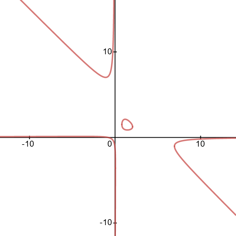
Figure 2: The Somos-5 curve (2.39)

2.3 QRT maps from Somos-5 sequences

QRT maps, named after Quispel, Roberts and Thompson, are an 18-parameter family of birational maps of the plane that were introduced in [45] in order to unify various functional equations and maps appearing in statistical mechanics, dynamical systems and discrete soliton theory [46]. They are integrable maps in the sense of [5, 42, 54], having an invariant symplectic form and a conserved quantity, and can be defined intrinsically starting from families of plane biquadratic curves, with associated elliptic fibrations of rational surfaces [12, 52]. The Somos-5 sequences (1.14) and (1.15) both generate particular orbits of the same QRT map, which is obtained by considering the ratios

$$u_{n}=\frac{S_{n-2}S_{n+1}}{S_{n-1}S_{n}},\qquad v_{n}=\frac{T_{n-2}T_{n+1}}{T_{n-1}T_{n}}.$$ (2.36)

These two sets of rational numbers both satisfy the same rational recurrence relation of order two, that is

$$u_{n+1}u_{n-1}=1+\frac{1}{u_{n}},\qquad v_{n+1}v_{n-1}=1+\frac{1}{v_{n}},$$ (2.37)

and the conserved quantity (2.4) for Somos-5 can be rewritten in terms of these ratios, leading to a conserved quantity for the rational recurrence in the form

$$\tilde{J}=u_{n}+u_{n-1}+\frac{1}{u_{n}}+\frac{1}{u_{n-1}}+\frac{1}{u_{n}u_{n-1}},$$ (2.38)

with the initial conditions $u_{0}=u_{1}=1$ giving $\tilde{J}=5$ in this case. (The other conserved quantity (2.3) cannot be reduced to a function of these ratios.) In other words, the sequence of points $(U,V)=(u_{n},u_{n+1})$ lies on the cubic plane curve

$${\cal C}:\qquad U^{2}V+UV^{2}-5UV+U+V+1=0,$$ (2.39)

and the same is true for the sequence of points $(U,V)=(v_{n},v_{n+1})$; see Fig.2 for a plot of the real curve in ${\mathbb{R}}^{2}$. The curve (2.39) is just (2.7) with the particular values $\tilde{\alpha}=\tilde{\beta}=1$, $\tilde{J}=5$ for the coefficients: it is symmetric and biquadratic, so it admits the simple involutions

$$\iota:\,(U,V)\mapsto(V,U),\qquad\iota_{h}:\,(U,V)\mapsto(U^{\dagger},V),$$ (2.40)

where the horizontal switch $\iota_{h}$ is obtained by intersecting the curve with a horizontal line and replacing each point $(U,V)$ with the other point of intersection $(U^{\dagger},V)$, which from Vieta’s formula for the product of the roots of a quadratic is given by $UU^{\dagger}=1+1/V$. Thus we see that the rational recurrence (2.37) corresponds to a symmetric QRT map, being given by the composition $\varphi=\iota\circ\iota_{h}$ of these two involutions, which sends $(u_{n-1},u_{n})\mapsto(u_{n},u_{n+1})$; and although so far it has been defined only on one particular curve, it lifts to a birational map of the plane by taking the pencil of curves obtained by replacing $5\to\tilde{J}$ in (2.39). Moreover, by construction each orbit of $\varphi$ lies on one of these curves, which generically has genus one, and corresponds to a sequence of points $\hat{{\cal P}}_{0}+n{\cal P}$ (where $+$ denotes addition in the group law of the curve).

Table 5: The first few rational numbers in the sequences (2.36) and (2.41).

$n$	0	1	2	3	4	5	6	7	8	9
$u_{n}$	$1$	$1$	$2$	$\tfrac{3}{2}$	$\tfrac{5}{6}$	$\tfrac{22}{15}$	$\tfrac{111}{55}$	$\tfrac{415}{407}$	$\tfrac{3014}{3071}$	$\tfrac{45029}{22742}$
$v_{n}$	$\infty$	$\infty$	$0$	$-1$	$7$	$-\tfrac{8}{7}$	$\tfrac{1}{56}$	$-\tfrac{399}{8}$	$\tfrac{3128}{57}$	$-\tfrac{455}{22287}$
$f_{n}$	$\infty$	$1$	$-1$	$2$	$3$	$-\tfrac{5}{7}$	$\tfrac{11}{8}$	$-37$	$-\tfrac{83}{57}$	$\tfrac{274}{391}$

In what follows, an important role will be played by the ratio

$$f_{n}=\frac{S_{n}}{T_{n}},$$ (2.41)

which turns out to lead to a QRT map on a different biquadratic curve, related to (2.39) by a 2-isogeny.

Proposition 2.19.

The ratio of the two Somos-5 sequences, given by (2.41), can be written as

$$f_{n}=\begin{cases}-\Phi(n{\kappa})/\Phi(2{\kappa}),&\text{for }n\,\,\mathrm{even}\\ \Phi(n{\kappa})/\Phi({\kappa}),&\text{for }n\,\,\mathrm{odd},\end{cases}$$ (2.42)

where

$$\Phi(z)=\frac{{\sigma}(z+{\omega})e^{-\eta z}}{{\sigma}({\omega}){\sigma}(z)},$$ (2.43)

with $\eta=\zeta({\omega})$ being the Weierstrass zeta function evaluated at the half-period ${\omega}$ of the curve (2.9) with invariants as in (2.18). The sequence of ratios satisfies the recurrence

$$f_{n+1}f_{n-1}=\begin{cases}(1+f_{n}^{2})/(2-f_{n}^{2}),&\text{for }n\,\,\mathrm{even}\\ (1+2f_{n}^{2})/(1-f_{n}^{2}),&\text{for }n\,\,\mathrm{odd},\end{cases}$$ (2.44)

and for all $j\in{\mathbb{Z}}$ the points $(W,Z)=(f_{2j\pm 1},f_{2j})$ lie on the biquadratic plane curve

$$(1-W^{2})Z^{2}+3WZ+2W^{2}+1=0,$$ (2.45)

corresponding to an orbit of a QRT map associated with this curve.

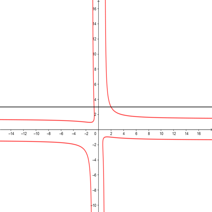
Figure 3: The curve (2.45) in the $(W,Z)$ plane intersecting the horizontal line $Z=3$ in two points.

• We begin by recalling some of the properties of the function $\Phi(z)$, which is well known as a solution of the simplest case of Lamé’s equation, in the form of a Schrödinger equation with an elliptic potential, i.e. it satisfies the differential equation $\Phi^{\prime\prime}(z)-2\wp(z)\Phi(z)=\wp({\omega})\Phi(z)$. From the quasiperiodicity of the sigma function it follows that $\Phi(z)$ is an odd function, and it is periodic with respect to the period $2{\omega}$ but acquires a minus sign when shifted by the real/imaginary periods $2{\omega}_{1},2{\omega}_{2}$; we record these properties, and its behaviour under a shift by ${\omega}$, as follows:

  $$\Phi(-z)=-\Phi(z),\quad\Phi(z+{\omega})=-\frac{e^{\eta{\omega}}}{{\sigma}({\omega})^{2}\Phi(z)},\quad\Phi(z+2{\omega})=\Phi(z),\quad\Phi(z+2{\omega}_{j})=-\Phi(z),\,\,\mathrm{for}\,\,j=1,2.$$ (2.46)

  Using the fact that $\Phi$ is odd, together with the standard identity

  $$\frac{{\sigma}(w+z){\sigma}(w-z)}{{\sigma}(w)^{2}{\sigma}(z)^{2}}=\wp(z)-\wp(w),$$ (2.47)

  valid for any $z,w\in{\mathbb{C}}$ (away from poles), it is apparent that

  $$\Phi(z)^{2}=\wp(z)-\wp({\omega}),$$ (2.48)

  and since $g_{2},g_{3}$ and $\wp({\omega})$ as in (2.18) and (2.21) are all real, $\Phi(z)\sim 1/z$ as $z\to 0$, and $\Phi$ has no real zeros, it follows that $\Phi(z)$ is real-valued for $z\in{\mathbb{R}}$, with $\Phi(z)>0$ for $0<z<2{\omega}_{1}$ and $\Phi(z)<0$ for $-2{\omega}_{1}<z<0$. Then since, from (2.20), ${\kappa}$ is negative and $-2{\omega}_{1}<2{\kappa}<0$, this allows us to compute

  $$\Phi({\kappa})=-\sqrt{\wp({\kappa})-\wp({\omega})}=-\frac{\sqrt{2}}{6^{\frac{1}{4}}},\quad\Phi(2{\kappa})=-\sqrt{\wp(2{\kappa})-\wp({\omega})}=-\frac{1}{6^{\frac{1}{4}}},$$ (2.49)

  where we have used the values of the $\wp$ function in (2.18) and (2.21), as well as the fact that

  $$\wp(2{\kappa})=\wp({\kappa})-\frac{{\sigma}(3{\kappa})}{{\sigma}(2{\kappa})^{2}{\sigma}({\kappa})}=\wp({\kappa})-\frac{\mathrm{a}_{3}}{\mathrm{a}_{2}^{2}}=\tilde{{\lambda}}-\frac{\tilde{\alpha}}{\tilde{\mu}^{2}}=\frac{17}{12\sqrt{6}},$$

  which follows from (2.47) together with the appropriate expressions for the terms of the companion EDS $(\mathrm{a}_{n})$ defined by (2.14). Now for even $n=2k$ we can calculate the ratio (2.41) using (2.17) and (2.26), to find

  $$f_{n}=-\frac{B_{+}^{k}\,\mu^{k^{2}}{\sigma}(n{\kappa}+{\omega}){\sigma}(2{\kappa})}{\hat{B}_{-}^{k-1}\,\mu^{(k-1)^{2}}{\sigma}(n{\kappa}){\sigma}({\omega})}=-\Phi(n{\kappa})\,\left(\frac{B_{+}}{\hat{B}_{-}}\,\mu^{2}e^{2\eta{\kappa}}\right)^{k}\frac{\hat{B}_{-}{\sigma}(2{\kappa})}{\mu},$$

  and then note that from (2.19) we may write

  $$B_{+}=-\frac{{\sigma}({\kappa})^{4}e^{-2\eta{\kappa}}}{{\sigma}(2{\kappa})\Phi(2{\kappa})}=-\frac{e^{-2\eta{\kappa}}}{\mathrm{a}_{2}\Phi(2{\kappa})}=\frac{e^{-2\eta{\kappa}}}{\tilde{\mu}\Phi(2{\kappa})}=-e^{-2\eta{\kappa}},$$

  taking the value of $\Phi(2{\kappa})$ as in (2.49), with $\tilde{\mu}=6^{\frac{1}{4}}$, so by (2.27) the expression in round brackets with exponent $k$ above is $B_{+}\mu^{2}e^{2\eta{\kappa}}/\hat{B}_{-}=1$, while the ratio appearing to the right of the round brackets is $\hat{B}_{-}{\sigma}(2{\kappa})/\mu=-\tilde{\mu}=1/\Phi(2{\kappa})$, thus indeed this yields $f_{n}=-\Phi(n{\kappa})/\Phi(2{\kappa})$ for even $n$, as required. Similarly, for odd $n=2k+1$ we find

  $$f_{n}=\frac{B_{-}^{k}{\sigma}(n{\kappa}+{\omega}){\sigma}({\kappa})}{\hat{B}_{+}^{k}{\sigma}(n{\kappa}){\sigma}({\kappa}+{\omega})}=\frac{\Phi(n{\kappa})}{\Phi({\kappa})}\left(\frac{B_{-}e^{2\eta{\kappa}}}{\hat{B}_{+}}\right)^{k},$$

  but then by (2.13) and (2.27) we see that $B_{-}e^{2\eta{\kappa}}/\hat{B}_{+}=-\mu B_{+}e^{2\eta{\kappa}}/\mu=1$, so this reduces to the required formula in (2.42) when $n$ is odd. Then to obtain the recurrence (2.44), let us write $f_{n}=C_{\pm}\Phi(n{\kappa})$ for appropriate constants $C_{\pm}$ depending on the parity of $n$, as in (2.42), so that the left-hand side of the recurrence is given by $f_{n+1}f_{n-1}=C_{\mp}^{2}\Phi(n{\kappa}+{\kappa})\Phi(n{\kappa}-{\kappa})$ for even/odd $n$ respectively. Hence, by substituting the appropriate ratios of sigma functions and applying (2.47) to the numerator and denominator, this gives

  $$f_{n+1}f_{n-1}=C_{\mp}^{2}e^{-2\eta n{\kappa}}\frac{{\sigma}(n{\kappa}+{\omega})^{2}\big{(}\wp({\kappa})-\wp(n{\kappa}+{\omega})\big{)}}{{\sigma}(n{\kappa})^{2}\big{(}\wp({\kappa})-\wp(n{\kappa})\big{)}}.$$

  The function $\wp(z+{\omega})$ is an even elliptic function of order two with double poles at $z\equiv{\omega}\bmod\Lambda$, where $\Lambda=2{\omega}_{1}{\mathbb{Z}}\oplus 2{\omega}_{2}{\mathbb{Z}}$ is the period lattice of the curve (2.9) with invariants $g_{2},g_{3}$ as in (2.18), hence it can be written in the form $\wp(z+{\omega})=\big{(}A^{\prime}\wp(z)+B^{\prime}\big{)}/\big{(}\wp(z)-\wp({\omega})\big{)}$ for suitable constants $A^{\prime},B^{\prime}$, and the leading (constant) term in the Taylor expansion at $z=0$ gives $A^{\prime}=\wp({\omega})$; the value of $B^{\prime}$ can be fixed from the $O(z^{2})$ term in the expansion, or by using the addition formula for the $\wp$ function, but will not be needed here. Thus, for another constant $B^{\prime\prime}$, we may write

  $$f_{n+1}f_{n-1}=C_{\mp}^{2}\Phi(n{\kappa})^{2}\frac{\big{(}\Phi({\kappa})^{2}+B^{\prime\prime}\Phi(n{\kappa})^{-2}\big{)}}{\big{(}\Phi({\kappa})^{2}-\Phi(n{\kappa})^{2}\big{)}}=C_{\mp}^{2}\frac{\big{(}\Phi({\kappa})^{2}C_{\pm}^{-2}f_{n}^{2}+B^{\prime\prime}\big{)}}{\big{(}\Phi({\kappa})^{2}-C_{\pm}^{-2}f_{n}^{2}\big{)}}.$$

  Using the fact that $C_{+}=-\Phi(2{\kappa})^{-1}$, $C_{-}=\Phi({\kappa})^{-1}$ and the values $f_{1}=-f_{2}=1$, $f_{3}=2$, we immediately find $B^{\prime\prime}=\frac{1}{2}\Phi({\kappa})^{4}$ from the $n=2$ case of this relation, and this fixes the recurrence in the form (2.44) for even/odd $n$ respectively. If we start from the pencil of biquadratic curves $(1-W^{2})Z^{2}+\hat{J}WZ+2W^{2}+1=0$, with arbitrary parameter $\hat{J}$, then the horizontal switch $\bar{\iota}_{h}:\,(W,Z)\mapsto(W^{\dagger},Z)$ corresponds to the formula (2.44) for even $n$, which sends $(f_{2j-1},f_{2j})\mapsto(f_{2j+1},f_{2j})$, and the vertical switch $\bar{\iota}_{v}:\,(W,Z)\mapsto(W,Z^{\dagger})$ corresponds to the case of odd $n$, which sends $(f_{2j+1},f_{2j})\mapsto(f_{2j+1},f_{2j+2})$, while the composition of these two involutions is a QRT map of general type, $\varphi_{QRT}=\bar{\iota}_{v}\circ\bar{\iota}_{h}$. The initial values $f_{1}=-f_{2}=1$ fix the value $\hat{J}=3$, giving an orbit that lies on the curve (2.45), which is illustrated in Fig.3, showing the horizontal line for the switch $\bar{\iota}_{h}:\,(2,3)\mapsto\big{(}-\tfrac{5}{7},3\big{)}$ corresponding to $n=4$ in (2.44). ∎

Proposition 2.20.

There is a 2-isogeny relating the the curve (2.45) to (2.39).

• The 2-isogeny relating the curve (2.45) to (2.39), or equivalently to the corresponding Weierstrass curve (2.9), can be seen in various ways. First of all, note that the function $\Phi(z)$ is not an elliptic function with respect to the original period lattice $\Lambda$, which is generated by the periods $2{\omega}$ and $2{\omega}_{2}$, but it is elliptic with respect to the lattice generated by $2{\omega}$ and $4{\omega}_{2}$; so if we set $\tau={\omega}_{2}/{\omega}$ and start with the normalized lattice with generators $1,\tau$, then the new lattice has generators $1,2\tau$, and the overall effect is the period doubling $\tau\mapsto 2\tau$, corresponding to what is known classically as the Landen transformation (see chapter XXII in [56], or [1] and references). At the level of the curves, this can be seen by computing $\rho$, the cross-ratio of the three roots of the cubic in (2.23) together with $\infty$, which allows the j-invariant to be calculated as

  $$j=\frac{256(\rho^{2}-\rho+1)^{3}}{\rho^{2}(\rho-1)^{2}}=\frac{11^{6}}{612}.$$ (2.50)

  Then for the new curve related by the Landen transformation, we have that

  $$\rho^{*}=\frac{4\sqrt{\rho}}{(1+\sqrt{\rho})^{2}}$$

  gives (an appropriate choice of) the value of the cross-ratio of the roots of the quartic in the equation

  $$\bar{y}^{2}=8W^{4}+5W^{2}-4,$$ (2.51)

  which is birationally equivalent to (2.45) via the transformation

  $$Z=\frac{-3W+\bar{y}}{2(1-W^{2})},$$

  from which one finds the j-invariant

  $$j^{*}=\frac{256((\rho^{*})^{2}-\rho^{*}+1)^{3}}{(\rho^{*})^{2}(\rho^{*}-1)^{2}}=\frac{16(\rho^{2}+14\rho+1)^{3}}{\rho(\rho-1)^{4}}=\frac{46268279}{46818}.$$

  Another indirect check is provided by verifying that the corresponding Hauptmoduls $\mathrm{x}=1728/j$, $\mathrm{y}=1728/j^{*}$ are the coordinates of a point on the modular curve

  $$1953125\mathrm{x}^{3}\mathrm{y}^{3}-187500\mathrm{x}^{2}\mathrm{y}^{2}(\mathrm{x}+\mathrm{y})+375\mathrm{x}\mathrm{y}\textperiodcentered(16\mathrm{x}^{2}-4027\mathrm{x}\mathrm{y}+16\mathrm{y}^{2})-64(\mathrm{x}+\mathrm{y})(\mathrm{x}^{2}+1487\mathrm{x}\mathrm{y}+\mathrm{y}^{2})+110592\mathrm{x}\mathrm{y}=0.$$

  These checks all confirm that there is a 2-isogeny over ${\mathbb{C}}$, but to establish this over ${\mathbb{Q}}$ we provide a direct transformation of coordinates, given by the formulae

  $$x^{*}=W^{2},\qquad y^{*}=(1-W^{2})WZ+\frac{3}{2}W^{2},$$ (2.52)

  which transforms (2.45) to the cubic

  $$4(y^{*})^{2}=8(x^{*})^{3}+5(x^{*})^{2}-4x^{*},$$

  and after shifting $x^{*}\to x^{*}-5/24$ and rescaling $x^{*}$ and $y^{*}$ by suitable powers of 2 this is seen to be equivalent to (2.23). ∎

Remark 2.21.

The primes appearing in the factorization of the denominator of (2.50), $612=2^{2}\cdot 3^{2}\cdot 17$, are the primes of bad reduction, which we will return to at the end of the next section.

3 Proof of main results

In order to prove our main theorem, we must first show that there is an infinite sequence of pairs of positive points $(M_{a},P_{a},X_{a})$, $(M_{b},P_{b},X_{b})$ lying on the Schubert surface (1.5), so that

$$M_{a}-{M_{a}}^{-1}=P_{a}-{P_{a}}^{-1}+2\left(X_{a}-{X_{a}}^{-1}\right),$$ (3.1)

$$M_{b}-{M_{b}}^{-1}=P_{b}-{P_{b}}^{-1}+2\left(X_{b}-{X_{b}}^{-1}\right),$$ (3.2)

and these sets of Schubert parameters are compatible in the sense that

$$\frac{2(X_{a}+X_{a}^{-1})}{P_{a}+P_{a}^{-1}}=\frac{P_{b}+P_{b}^{-1}}{M_{b}+M_{b}^{-1}}=\frac{a}{c},$$ (3.3)

$$\frac{M_{a}+M_{a}^{-1}}{P_{a}+P_{a}^{-1}}=\frac{2(X_{b}+X_{b}^{-1})}{M_{b}+M_{b}^{-1}}=\frac{b}{c},$$ (3.4)

which serves as the definition of the ratios $a/c$, $b/c$, and hence (up to scale) defines the associated Heron triangle with two rational medians. As the main initial step, we begin by giving a proof of the empirical observation of Buchholz and Rathbun in [7] that there is an infinite sequence of Schubert parameters with signs, given in terms of the two Somos-5 sequences by (1.12) and (1.13), or equivalently in terms of the rational sequences $(u_{n})$, $(v_{n})$ and $(f_{n})$ by

$$M_{a,n}=-\frac{f_{n+1}f_{n+2}^{2}}{f_{n}},\quad P_{a,n}=-\frac{1}{u_{n+2}v_{n+2}},\quad X_{a,n}=2^{(-1)^{n+1}}\frac{f_{n}f_{n+2}^{2}}{f_{n+3}},$$ (3.5)

$$M_{b,n}={u_{n+3}v_{n+3}},\quad P_{b,n}=-\frac{f_{n+2}^{2}f_{n+3}}{f_{n+4}},\quad X_{b,n}=2^{(-1)^{n}}\frac{f_{n+1}}{f_{n+2}^{2}f_{n+4}}.$$ (3.6)

Having proved that these formulae give points on the Schubert surface satisfying the necessary constraints, we will then show that the pattern of signs varies coherently with $n$ in such a way that replacing any negative parameter by minus its reciprocal will preserve the constraints and hence provide, for each $n$, two compatible sets of positive Schubert parameters. Then finally we will be able to verify the formulae for $a,b,c,k,\ell$ and $\Delta$ in Theorem 1.2.

Before tackling the Schubert parameters with signs, we introduce the sequence of quantities

$$\begin{array}[]{rl}\bar{s}_{n}=-S_{n+3}S_{n+4}^{2}T_{n}^{2}T_{n+1},&\bar{a}_{n}=-S_{n+2}T_{n+1}T_{n+2}^{3}T_{n+3},\\ \bar{b}_{n}=S_{n+1}S_{n+2}^{3}S_{n+3}T_{n+2},&\bar{c}_{n}=S_{n}^{2}S_{n+1}T_{n+3}T_{n+4}^{2},\end{array}$$ (3.7)

which we will refer to as the signed lengths. After taking absolute values, for each $n$ there is an equality of sets of positive numbers:

$$\{\,|\bar{s}_{n}|,|\bar{a}_{n}|,|\bar{b}_{n}|,|\bar{c}_{n}|\,\}=\{\,s,s-a,s-b,s-c\,\}.$$

When $n=1$ the choice of signs in (3.7) ensures that $\bar{s}_{1},\bar{a}_{1},\bar{b}_{1}$ and $\bar{c}_{1}$ are all positive, and coincide with $s,s-a,s-b$ and $s-c$, respectively (see Table 6), but it turns out that in general the signed lengths correspond to a permutation of the latter four quantities with signs, in a pattern that repeats with period 14. Nevertheless, the pattern of permutations and signs respects the linear relation

$$s=(s-a)+(s-b)+(s-c)$$

that holds between their associated positive counterparts.

Table 6: The first few signed lengths.

$n$	0	1	2	3	4	5	6	7
$\bar{s}_{n}$	$0$	$75$	$-605$	$-15059$	$1784251$	$-2442672736$	$25972376704$	$2633103021849$
$\bar{a}_{n}$	$1$	$2$	$21$	$13720$	$-39424$	$-16872$	$-6010068429$	$-424782960455490$
$\bar{b}_{n}$	$-2$	$24$	$270$	$-28875$	$1969880$	$-46246189$	$-330416266542$	$812450885698024$
$\bar{c}_{n}$	$1$	$49$	$-896$	$96$	$-146205$	$-2396409675$	$362398711675$	$-385034822220685$

Lemma 3.1.

The signed lengths (3.7) satisfy

$$\bar{s}_{n}=\bar{a}_{n}+\bar{b}_{n}+\bar{c}_{n}$$ (3.8)

for all $n\in{\mathbb{Z}}$.

• The equation (3.8) is a degree 6 linear relation between products of terms of the Somos sequences $(S_{n})$ and $(T_{n})$, but has a different form compared with the identities for minors proved in Proposition 2.10. Upon rearranging and dividing both sides by $\bar{a}_{n}$, it can be rewritten as

  $$1-f_{n+1}f_{n+2}^{2}f_{n+3}=(v_{n+2}v_{n+3})^{2}\left(\frac{f_{n}^{2}f_{n+1}+f_{n+3}f_{n+4}^{2}}{f_{n+2}}\right).$$ (3.9)

  The latter identity relates the rational sequences $(v_{n})$ and $(f_{n})$ corresponding to particular orbits of the two different QRT maps (2.37) and (2.44); alternatively, it could be written in terms of $(u_{n})$ and $(f_{n})$, since the ratio $u_{n}/v_{n}$ can be expressed in terms of the $f_{n}$. It is equivalent to an identity between elliptic functions, since $f_{n}$ is given by the formula (2.42), and $v_{n}$ is given by a ratio of Somos-5 terms as in (2.36), which are themselves given in analytic form by (2.26). Hence, in order to prove it, we set $z=(n+2){\kappa}$, so that the left-hand side above can be written as

  $$1-\frac{\Phi(z-{\kappa})\Phi(z+{\kappa})\big{(}\wp(z)-\wp({\omega})\big{)}}{\Phi({\kappa})^{2}\Phi(2{\kappa})^{2}},$$ (3.10)

  while the right-hand side is given by

  $$\frac{\tilde{\mu}^{4}\big{(}\wp(z)-\wp(2{\kappa})\big{)}^{2}\,\Phi(z+{\omega})\,\Big{(}\Phi(z-{\kappa})\big{(}\wp(z-2{\kappa})-\wp({\omega})\big{)}+\Phi(z+{\kappa})\big{(}\wp(z+2{\kappa})-\wp({\omega})\big{)}\Big{)}}{e^{\eta{\omega}}{\sigma}({\omega})^{-2}\Phi({\kappa})\Phi(2{\kappa})},$$ (3.11)

  where we have used (2.47) to simplify the ratio of sigma functions in $v_{n+2}v_{n+3}$, together with (2.48) and the expression for the reciprocal of $\Phi$ in (2.46). Both (3.10) and (3.11) are even elliptic functions of $z$, so to verify their equality it is sufficient to check that they have poles in the same places with the same singular part of the Laurent expansion around each pole, and agree at one finite value, since their difference is then an elliptic function without poles and therefore constant, and if they take the same finite value somewhere then this constant must be $0$. The left-hand side has double poles for $z\equiv 0\bmod\Lambda$, and for $z\to 0$ we have $\Phi(z-{\kappa})\Phi(z+{\kappa})=-\Phi({\kappa})^{2}+O(z^{2})$ and $\wp(z)=1/z^{2}+O(z^{2})$, so its Laurent expansion around the origin is $\Phi(2{\kappa})^{-2}/z^{2}+O(1)$. On the right-hand side, note that

  $$\Phi(z\pm{\kappa})\big{(}\wp(z\pm 2{\kappa})-\wp({\omega})\big{)}=\pm\Phi({\kappa})\big{(}\wp(2{\kappa})-\wp({\omega})\big{)}+C^{\prime}z+O(z^{2}),$$

  where $C^{\prime}=\big{(}\Phi^{\prime}({\kappa})\big{(}\wp(2{\kappa})-\wp({\omega})\big{)}+\Phi({\kappa})\wp^{\prime}(2{\kappa})\big{)}$, so the sum of these two terms gives an odd function with Taylor expansion $2C^{\prime}z+O(z^{3})$ at the origin, while $\Phi({\omega})=0$ and we have $\Phi(z+{\omega})=\Phi^{\prime}({\omega})z+O(z^{3})$. Hence to leading order, the expansion of the right-hand side around $z=0$ is $C/z^{2}+O(1)$, where

  $$C=\frac{2e^{-\eta{\omega}}{\sigma}({\omega})^{2}\tilde{\mu}^{4}\Big{(}\Phi^{\prime}({\kappa})\big{(}\wp(2{\kappa})-\wp({\omega})\big{)}+\Phi({\kappa})\wp^{\prime}(2{\kappa})\Big{)}\Phi^{\prime}({\omega})}{\Phi({\kappa})\Phi(2{\kappa})}.$$

  Now from (2.48) it follows that $2\Phi\Phi^{\prime}=\wp^{\prime}$, so $\Phi^{\prime}({\kappa})=\frac{1}{2}\wp^{\prime}({\kappa})/\Phi({\kappa})$, while putting $\Phi(z)=1/z+O(z)$ as $z\to 0$ into the identity $\Phi(z)\Phi(z+{\omega})=-e^{\eta{\omega}}{\sigma}({\omega})^{-2}$ gives $\Phi^{\prime}({\omega})=-e^{\eta{\omega}}{\sigma}({\omega})^{-2}$. Thus we have

  $$C\Phi(2{\kappa})^{2}=-2\Phi(2{\kappa})\tilde{\mu}^{4}\Big{(}\frac{1}{2}\Phi({\kappa})^{-2}\wp^{\prime}({\kappa})\big{(}\wp(2{\kappa})-\wp({\omega})\big{)}+\wp^{\prime}(2{\kappa})\Big{)}=\tilde{\mu}^{3}\left(\tilde{\mu}\Phi(2{\kappa})^{2}\Phi({\kappa})^{-2}-2\tilde{\mu}^{-3}\right),$$

  using (2.48) to replace the $\big{(}\wp(2{\kappa})-\wp({\omega})\big{)}$ term inside the large brackets, together with $\wp^{\prime}({\kappa})=\tilde{\mu}$ and $\wp^{\prime}(2{\kappa})={\sigma}(4{\kappa})/{\sigma}(2{\kappa})^{4}=\mathrm{a}_{4}/\mathrm{a}_{2}^{4}=-\tilde{\beta}/\tilde{\mu}^{3}=-\tilde{\mu}^{-3}$ from the formulae for the companion EDS, with $\tilde{\beta}=1$ in this case. Then substituting in $\tilde{\mu}=6^{\frac{1}{4}}$ and the values of $\Phi$ in (2.49) gives

  $$C\Phi(2{\kappa})^{2}=6\,\left(\frac{1/\sqrt{6}}{2/\sqrt{6}}\right)-2=1,$$

  so the singular parts of the Laurent expansions as $z\to 0$ are the same on each side of (3.9). Then (3.10) has poles at precisely two other places, namely simple poles for $z\equiv\pm{\kappa}\bmod\Lambda$ with residues

  $$\mp\frac{\Phi(2{\kappa})\big{(}\wp({\kappa})-\wp({\omega})\big{)}}{\Phi({\kappa})^{2}\Phi(2{\kappa})^{2}}=\mp\Phi(2{\kappa})^{-1},$$

  respectively, while in (3.11) we see simple poles at the same places, with the residues being

  $$\frac{e^{-\eta{\omega}}\tilde{\mu}^{4}\big{(}\wp({\kappa})-\wp(2{\kappa})\big{)}^{2}\,\Phi(\pm{\kappa}+{\omega})\,\big{(}\wp({\kappa})-\wp({\omega})\big{)}}{\Phi({\kappa})\Phi(2{\kappa})}=\mp\frac{\tilde{\mu}^{4}\big{(}\wp({\kappa})-\wp(2{\kappa})\big{)}^{2}\Phi({\kappa})^{2}}{\Phi({\kappa})^{2}\Phi(2{\kappa})}=\mp\frac{6\left(\frac{29}{12\sqrt{6}}-\frac{17}{12\sqrt{6}}\right)^{2}}{\Phi(2{\kappa})},$$

  i.e. equal to $=\mp\Phi(2{\kappa})^{-1}$, the same as for (3.10). The expression (3.11) also contains the terms $\wp(z\mp 2{\kappa})$ with double poles at $z\equiv\pm 2{\kappa}\mod\Lambda$, but these poles are cancelled by the prefactor $\big{(}\wp(z)-\wp(2{\kappa})\big{)}^{2}$ which has double zeros at these points; and there is also the term $\Phi(z+{\omega})$ which gives a simple pole for $z\equiv{\omega}\mod\Lambda$, but the factor that appears after it, evaluated at $z={\omega}$, yields

  $$\Phi({\omega}-{\kappa})\big{(}\wp({\omega}-2{\kappa})-\wp({\omega})\big{)}+\Phi({\omega}+{\kappa})\big{(}\wp({\omega}+2{\kappa})-\wp({\omega})\big{)}=\big{(}\Phi({\kappa}+{\omega})-\Phi({\kappa}-{\omega})\big{)}\big{(}\wp(2{\kappa}+{\omega})-\wp({\omega})\big{)}=0,$$

  from the periodicity of $\Phi$ and $\wp$ under shifts by $2{\omega}$ and the fact that these are odd/even functions, respectively, so this simple pole is cancelled by a zero. The values $n=-4,-3,-2,-1,0$ are all singular cases of (3.9), due to the presence of the term $f_{0}=\infty$: these give the values of $z$ corresponding to the poles, together with the removable singularities at $z=\pm 2{\kappa}$; but it is easy to check directly that (3.8) is satisfied for these values of $n$. The first nonsingular value is $n=1$, which corresponds to setting $z=3{\kappa}$, and from the values in Table 5 it is straightforward to check that the left-hand side and the right-hand side of (3.9) are both equal to $13$ in this case. Hence the functions (3.10) and (3.11) coincide, and the result follows. ∎

It appears that we have to prove four identities for the two sets of Schubert parameters with signs: two copies of the equation for the Schubert surface, and two constraints between the two sets of parameters. Moreover, (3.3) and (3.4) each contain two equalities, so upon replacing the ratios $a/c$ and $b/c$ by appropriate combinations of signed lengths, this gives a further two identities that must be verified. However, there is a symmetry to the problem which cuts the amount of work down by half.

Lemma 3.2.

Under the involution $n\to-n-4$, the Schubert parameters with signs transform as

$$M_{a,-n-4}=P_{b,n},\qquad P_{a,-n-4}=-1/M_{b,n},\qquad X_{a,-n-4}=1/X_{b,n},$$ (3.12)

and the signed lengths transform as

$$\bar{s}_{-n-4}=\bar{c}_{n},\quad\bar{a}_{-n-4}=-\bar{a}_{n},\quad\bar{b}_{-n-4}=-\bar{b}_{n},\quad\bar{c}_{-n-4}=\bar{s}_{n}.$$ (3.13)

• As already noted previously, the sequences (1.14) and (1.15) extend to all $n\in{\mathbb{Z}}$ in a way that is respectively symmetric/antisymmetric about $n=0$, so that

  $$S_{-n}=S_{n},\qquad T_{-n}=-T_{n}.$$

  For the corresponding rational sequences defined by (2.36) and (2.41), this implies immediately that

  $$u_{1-n}=u_{n},\qquad v_{1-n}=v_{n},\qquad f_{-n}=-f_{n},$$

  and then for $n\to-n-4$ it follows from (3.5) and (3.6) that the Schubert parameters transform according to (3.12). For the signed lengths, we have

  $$\bar{s}_{-n-4}=-S_{-n-1}S_{-n}^{2}T_{-n-4}^{2}T_{-n-3}=-S_{n+1}S_{n}^{2}(-T_{n+4})^{2}(-T_{n+3})=\bar{c}_{n},$$

  and similarly for the other three. ∎

Now starting from the Schubert equation (3.1) for $(M_{a},P_{a},X_{a})$ and replacing $M_{a}\to P_{b}$, $P_{a}\to-M_{b}^{-1}$, $X_{a}\to X_{b}^{-1}$ gives $P_{b}-P_{b}^{-1}=-M_{b}^{-1}+M_{b}+2(X_{b}^{-1}-X_{b})$, which is just a rearrangement of (3.2), and if at the same time we replace $P_{b}\to M_{a}$, $M_{b}\to-P_{a}^{-1}$, $X_{b}\to X_{a}^{-1}$ then it is clear that these two copies of Schubert’s equation are switched. Similarly, applying this involution to the first equality in (3.3) gives the first equality in (3.4), up to an overall minus sign, and vice versa. Furthermore, we can apply this symmetry to the second equality in (3.3) by interpreting the right-hand side suitably in terms of the signed lengths, so that (omitting the index $n$) we may write

$$\frac{P_{b}+P_{b}^{-1}}{M_{b}+M_{b}^{-1}}=\frac{\bar{s}-\bar{a}}{\bar{s}-\bar{c}},$$ (3.14)

and then applying the involution to the Schubert parameters on the left, as well as $\bar{s}\to\bar{c}$, $\bar{a}\to-\bar{a}$, $\bar{c}\to\bar{s}$ on the right, this becomes

$$-\frac{M_{a}+M_{a}^{-1}}{P_{a}+P_{a}^{-1}}=\frac{\bar{c}+\bar{a}}{\bar{c}-\bar{s}},$$

but then applying the first equality in (3.4) together with Lemma 3.1, this implies

$$\frac{2(X_{b}+X_{b}^{-1})}{M_{b}+M_{b}^{-1}}=\frac{\bar{s}-\bar{b}}{\bar{s}-\bar{c}},$$ (3.15)

which is just the second equality in (3.4), with the right-hand side written in terms of the signed lengths. Hence we see that for the the Schubert parameters with signs and the signed lengths, the involution $n\to-n-4$ interchanges the two copies of Schubert’s equation, and the two pairs of equalities given by the constraints (3.3) and (3.4), so it is equivalent to switching $a\leftrightarrow b$ in each triangle. Thus it is sufficient to prove (3.1) and the two equalities in (3.3) for all integer values of $n$, and the other relations follow by symmetry.

Theorem 3.3.

The two sets of Schubert parameters with signs, that is $(M_{a,n},P_{a,n},X_{a,n})$, $(M_{b,n},P_{b,n},X_{b,n})$ given by (3.5) and (3.6), satisfy the relations (3.1), (3.2), (3.3) and (3.4) for all $n\in{\mathbb{Z}}$, where the quantities on the right-hand sides of (3.3) and (3.4) should be interpreted in terms of the signed lengths as

$$\frac{\bar{s}_{n}-\bar{a}_{n}}{\bar{s}_{n}-\bar{c}_{n}}\qquad and\qquad\frac{\bar{s}_{n}-\bar{b}_{n}}{\bar{s}_{n}-\bar{c}_{n}},$$

respectively.

• From (3.5) we may set $z=(n+2){\kappa}$ and write

  $$\begin{array}[]{l}M_{a,n}=-C_{+}C_{-}\tilde{\gamma}\Phi(z-{\kappa})\Phi(z)^{2}\Phi(z-2{\kappa}+{\omega}),\\ P_{a,n}=-\mu^{-2}{\sigma}(z-{\kappa}+{\omega}){\sigma}(z+{\omega}){\sigma}(z-{\kappa}){\sigma}(z)/\big{(}{\sigma}(z-2{\kappa}+{\omega}){\sigma}(z+{\kappa}+{\omega}){\sigma}(z-2{\kappa}){\sigma}(z+{\kappa})\big{)},\\ X_{a,n}=2^{\mp 1}C_{\pm}^{3}C_{\mp}^{-1}\tilde{\gamma}\Phi(z-2{\kappa})\Phi(z)^{2}\Phi(z+{\kappa}+{\omega}),\end{array}$$ (3.16)

  for even/odd $n$, respectively, where we have used (2.46) with the same notation as in the proof of Proposition (2.19), and for convenience we have written the residue of $\Phi(z)^{-1}$ at $z=-{\omega}$ as

  $$\tilde{\gamma}=-e^{-\eta{\omega}}{\sigma}({\omega})^{2}=\underset{z\to-{\omega}}{\rm lim}\frac{(z+{\omega})}{\Phi(z)},$$ (3.17)

  namely the multiplier that appears when the reciprocal of $\Phi$ is replaced by the same function shifted by ${\omega}$. The above formula for $P_{a,n}$ is a consequence of (2.17) and (2.26), which imply that

  $$u_{n}=\left(\frac{B_{\mp}}{B_{\pm}}\right)\mu^{1\mp 1}\,\frac{{\sigma}(z-2{\kappa}+{\omega}){\sigma}(z+{\kappa}+{\omega})}{{\sigma}(z-{\kappa}+{\omega}){\sigma}(z+{\omega})},\quad v_{n}=\left(\frac{\hat{B}_{\pm}}{\hat{B}_{\mp}}\right)\mu^{1\pm 1}\,\frac{{\sigma}(z-2{\kappa}){\sigma}(z+{\kappa})}{{\sigma}(z-{\kappa}){\sigma}(z)},$$

  for even/odd $n$, and the prefactors in brackets cancel in the product $u_{n}v_{n}$, due to (2.13) and (2.27). From these expressions, we see that $M_{a,n}$ has poles at $z\equiv 0,{\kappa},2{\kappa}+{\omega}$ modulo the period lattice $\Lambda$, while $M_{a,n}^{-1}$ has poles at $z\equiv{\omega},{\kappa}+{\omega},2{\kappa}$, $P_{a,n}$ has poles at $z\equiv-{\kappa},-{\kappa}+{\omega},2{\kappa},2{\kappa}+{\omega}$, while $P_{a,n}^{-1}$ has poles at $z\equiv 0,{\omega},{\kappa},{\kappa}+{\omega}$, and $X_{a,n}$ has poles at $z\equiv 0,2{\kappa},2,-{\kappa}+{\omega}$, while $X_{a,n}^{-1}$ has poles at $z\equiv{\omega},2{\kappa}+{\omega},-{\kappa}$. Then to verify that $(M_{a,n},P_{a,n},X_{a,n})$ satisfies (3.1) for all $n$, it is sufficient to check that the two sides of the equation define the same elliptic functions of $z$, by checking that they agree in the singular parts of their Laurent expansions around the poles at all these places, and at one finite value. This is equivalent to saying that the formulae (3.16) define an analytic embedding of the elliptic curve in the Schubert surface, and this does not depend on the parity of $n$ because the expressions for $M_{a,n}$ and $P_{a,n}$ are manifestly the same for even/odd $n$, while for the coefficient in front of the $z$-dependent part of the formula for $X_{a,n}$ we find the identity $\frac{1}{2}C_{+}^{3}C_{-}^{-1}=2C_{-}^{3}C_{+}^{-1}$, that is equivalent to $(C_{+}/C_{-})^{4}=\big{(}\Phi({\kappa})/\Phi(2{\kappa})\big{)}^{4}=4$, which follows from (2.49). To show that these parameter triples satisfy (3.1), it is convenient to rewrite the equation, collecting the terms as

  $$(M_{a,n}-2X_{a,n})+(2X_{a,n}^{-1}-M_{a,n}^{-1})=P_{a,n}-P_{a,n}^{-1}.$$ (3.18)

  The first bracketed expression on the left-hand side above is given as a function of $z$ by

  $$F(z)=\Phi({\kappa})^{-1}\Phi(2{\kappa})^{-1}\Phi(z)^{2}G(z),$$

  where

  $$G(z)=\tilde{\gamma}\big{(}\Phi(z-{\kappa})\Phi(z-2{\kappa}+{\omega})+2\Phi(z-2{\kappa})\Phi(z+{\kappa}+{\omega})\big{)}=\frac{\Phi(z-{\kappa})}{\Phi(z-2{\kappa})}+2\frac{\Phi(z-2{\kappa})}{\Phi(z+{\kappa})},$$

  and around $z=0$ we have $\Phi(z)^{2}=1/z^{2}+O(1)$ and

  $$G(z)=\left(\frac{\Phi(-{\kappa})}{\Phi(-2{\kappa})}+2\frac{\Phi(-2{\kappa})}{\Phi({\kappa})}\right)+\left(\frac{\Phi^{\prime}(-{\kappa})}{\Phi(-2{\kappa})}-\frac{\Phi(-{\kappa})\Phi^{\prime}(-2{\kappa})}{\Phi(-2{\kappa})^{2}}+2\frac{\Phi^{\prime}(-2{\kappa})}{\Phi({\kappa})}-2\frac{\Phi(-2{\kappa})\Phi^{\prime}({\kappa})}{\Phi({\kappa})^{2}}\right)z+O(z^{2}),$$

  so from (2.49) we see that $G(0)=0$, and as $z\to 0$, $G(z)=C^{*}z+O(z^{2})$, with

  $$C^{*}=\Phi^{\prime}({\kappa})\left(-\Phi(2{\kappa})^{-1}+2\Phi(2{\kappa})\Phi({\kappa})^{-2}\right)+\Phi^{\prime}(2{\kappa})\left(2\Phi({\kappa})^{-1}+\Phi({\kappa})\Phi(2{\kappa})^{-2}\right)=-\sqrt{2}\tilde{\mu}^{-1},$$

  using $\Phi^{\prime}(2{\kappa})=\frac{1}{2}\wp^{\prime}(2{\kappa})/\Phi(2{\kappa})$ and the values of $\Phi({\kappa})$, $\Phi(2{\kappa})$ and $\wp^{\prime}(2{\kappa})$ as before. Hence $F(z)$ has a simple pole at $z=0$ with residue $-\Phi({\kappa})^{-1}\Phi(2{\kappa})^{-1}\sqrt{2}\tilde{\mu}^{-1}=-\tilde{\mu}=-6^{\frac{1}{4}}$, while on the right-hand side of (3.18), $-P_{a,n}^{-1}$ also has a simple pole there with residue

  $$\mu^{2}\frac{{\sigma}(-2{\kappa}+{\omega}){\sigma}({\kappa}+{\omega}){\sigma}(-2{\kappa}){\sigma}({\kappa})}{{\sigma}(-{\kappa}+{\omega}){\sigma}({\omega}){\sigma}(-{\kappa})},$$

  but using the oddness of the sigma function and its quasiperiodicity, e.g. ${\sigma}({\kappa}+{\omega})=-e^{2\eta{\kappa}}{\sigma}({\kappa}-{\omega})$, we may rewrite this residue as $\mu^{2}{\sigma}(2{\kappa})^{2}\Phi(2{\kappa})=-\tilde{\mu}$ by (2.12), so these two residues agree. Now a calculation of the effect of shifting the argument in the Schubert parameters by ${\omega}$ shows that, because the expressions for $M_{a}$ and $X_{a}$ are both quartic in $\Phi$ with prefactors $\mp C_{+}C_{-}\tilde{\gamma}$, respectively, they satisfy $M_{a,n}(z+{\omega})=(C_{+}C_{-}\tilde{\gamma})^{2}\tilde{\gamma}^{-4}M_{a,n}(z)^{-1}=\Phi({\kappa})^{-2}\Phi(2{\kappa})^{-2}\tilde{\gamma}^{-2}M_{a,n}(z)^{-1}$, and similarly $X_{a,n}(z+{\omega})=\Phi({\kappa})^{-2}\Phi(2{\kappa})^{-2}\tilde{\gamma}^{-2}X_{a,n}(z)^{-1}$. However, by (2.48) we see that

  $$\tilde{\gamma}^{2}=\underset{z\to-{\omega}}{\rm lim}\frac{(z+{\omega})^{2}}{\wp(z)-\wp({\omega})}=\frac{2}{\wp^{\prime\prime}({\omega})}=\frac{2}{6\wp({\omega})^{2}-\frac{1}{2}g_{2}}=-\frac{1}{2}\tilde{\mu}^{4}=-3,$$

  and the quasiperiodicity of the sigma function implies that $P_{a}$ is unchanged under shifting by this half-period. So overall, using (2.49) once more, we find

  $$M_{a,n}(z)^{-1}=-M_{a,n}(z+{\omega}),\qquad P_{a,n}(z)=P_{a,n}(z+{\omega}),\qquad X_{a,n}(z)^{-1}=-X_{a,n}(z+{\omega}).$$ (3.19)

  In particular, if we consider simple poles at $z=-{\omega}$, this implies that the residue of the second set of bracketed terms on the left-hand side of (3.18) is also equal to $-\tilde{\mu}$, and is the same as the residue of the term $-P_{a,n}^{-1}$ on the right-hand side. Next we consider $z={\kappa}$, and verify that both $M_{a,n}$ on the left-hand side and $-P_{a,n}^{-1}$ on the right-hand side of (3.18) have the same residue $\tilde{\mu}$ there. Also, at $z=-{\kappa}-{\omega}$, we see that the residue at the simple pole in $-2X_{a,n}$ is given by

  $$-2C_{+}C_{-}\tilde{\gamma}\Phi(-3{\kappa}-{\omega})\Phi(-{\kappa}-{\omega})^{2}=-2\tilde{\gamma}^{-2}\Phi({\kappa})^{-3}\Phi(2{\kappa})^{-1}\Phi(3{\kappa})^{-1}=\frac{4}{f_{3}}\tilde{\mu}^{-4}\Phi({\kappa})^{-4}\Phi(2{\kappa})^{-1}=-\frac{\tilde{\mu}}{2},$$

  and this is balanced by $\mathrm{res}\,P_{a,n}|_{z=-{\kappa}-{\omega}}$, for which we find the same value

  $$\mu^{-2}\frac{{\sigma}({\kappa}){\sigma}(2{\kappa}){\sigma}({\kappa}+{\omega}){\sigma}(2{\kappa}+{\omega})}{{\sigma}(3{\kappa}){\sigma}({\omega}){\sigma}(3{\kappa}+{\omega})}=\mu^{-2}\frac{{\sigma}({\kappa})^{2}{\sigma}(2{\kappa})^{2}\Phi({\kappa})\Phi(2{\kappa})}{{\sigma}(3{\kappa})^{2}\Phi(3{\kappa})}=\frac{\mathrm{a}_{2}^{2}\Phi(2{\kappa})}{\mathrm{a}_{3}^{2}f_{3}}=-\frac{\tilde{\mu}}{2}.$$

  Using (3.19), we see that the total residue at the simple pole at $z=2{\kappa}$ on the left-hand side of (3.18) comes from the combination $-M_{a,n}^{-1}-2X_{a,n}$, being given by

  $$-C_{+}C_{-}\tilde{\gamma}\Phi({\kappa}+{\omega})\Phi(2{\kappa}+{\omega})^{2}-2C_{+}C_{-}\tilde{\gamma}\Phi(2{\kappa})^{2}\Phi(3{\kappa}+{\omega})=\tilde{\gamma}^{-2}\Phi({\kappa})^{-2}\Phi(2{\kappa})^{-3}+2\Phi({\kappa})^{-2}\Phi(2{\kappa})f_{3}^{-1}=\frac{\tilde{\mu}}{2},$$

  and we find the same value for $\mathrm{res}\,P_{a,n}|_{z=2{\kappa}}$ on the right-hand side. The fact that the residues balance at the other poles at places congruent to $z={\kappa}+{\omega},-{\kappa},2{\kappa}+{\omega}$ modulo $\Lambda$ then follows immediately from the symmetry (3.19), and it is easy to see that the set of finite Schubert parameters $(4,\tfrac{2}{3},\tfrac{8}{3})$ for $n=1$, corresponding to the value $z=3{\kappa}$, is a point on the Schubert surface, so this completes the verification that (3.18) holds as an identity between elliptic functions of $z$, and in particular shows that (3.1) is satisfied for all $n$, and thus by the preceding lemma the second sequence of Schubert parameters satisfies (3.2) as well.

  Now to prove the first of the equalities in (3.3), we rewrite it as

  $$2(X_{a,n}+X_{a,n}^{-1})(M_{b,n}+M_{b,n}^{-1})=(P_{a,n}+P_{a,n}^{-1})(P_{b,n}+P_{b,n}^{-1}),$$ (3.20)

  where by Lemma 3.2 we see that the analytic expressions for $M_{b,n},P_{b,n},X_{b,n}$ are obtained by replacing $z\to-z$ in the formulae for $-P_{a,n}^{-1},M_{a,n},X_{a,n}^{-1}$, respectively, so from (3.16) we find

  $$\begin{array}[]{l}M_{b,n}=\mu^{2}{\sigma}(z-{\kappa}+{\omega}){\sigma}(z+2{\kappa}+{\omega}){\sigma}(z+2{\kappa}){\sigma}(z-{\kappa})/\big{(}{\sigma}(z+{\kappa}+{\omega}){\sigma}(z+{\omega}){\sigma}(z){\sigma}(z+{\kappa})\big{)},\\ P_{b,n}=-C_{+}C_{-}\tilde{\gamma}\Phi(z+{\kappa})\Phi(z)^{2}\Phi(z+2{\kappa}+{\omega}),\\ X_{b,n}=-C_{+}C_{-}\tilde{\gamma}\Phi(z+{\kappa})\Phi(z+{\omega})^{2}\Phi(z-2{\kappa}+{\omega}).\end{array}$$ (3.21)

  On each side of the relation (3.20), there are poles at all the same values of $z$ that were considered in the case of (3.1), as well as at points congruent to $z=-2{\kappa}$ and $z=-2{\kappa}-{\omega}$ modulo $\Lambda$. At $z=0$, there are poles of order 3 on each side, so that we should have $2X_{a}M_{b}\sim P_{b}P_{a}^{-1}$, so we need to show that

  $$2\big{(}X_{a,n}+O(z^{2})\big{)}(M_{b,n}+M_{b,n}^{-1})=\big{(}P_{b,n}+O(z^{2})\big{)}(P_{a,n}^{-1}+P_{a,n}),$$

  where the terms $M_{b,n}^{-1},P_{a,n}$ are corrections of $O(z)$, giving a term with a simple pole when they are multiplied by the triple pole in the first bracket on the left/right-hand side, respectively. The expansion around the triple pole is rather arduous, but the problem of showing that the two sides balance can be simplified by noting that, from (3.1) we have (omitting index $n$) $P_{a}^{-1}=2X_{a}-M_{a}+O(z)$, which we can use to replace the first term in the second bracket on the right above, and similarly in the second bracket on the left we can use $M_{b}=P_{b}-2X_{b}^{-1}+O(z)$ from (3.2), so that at leading order, the balancing of the two sides is equivalent to $2X_{a}(P_{b}-2X_{b}^{-1})\sim P_{b}(2X_{a}-M_{a})$, and we can cancel the term $2X_{a}P_{b}$ from each side. This may look like the problem has become more difficult, because we are left with a leading order pole of order 4 on each side, but in fact the singular terms that remain require that, as $z\to 0$,

  $$2X_{a,n}(-2X_{b,n}^{-1}+2M_{b,n}^{-1})\sim P_{b,n}(-M_{a,n}+2P_{a,n}),$$ (3.22)

  where all omitted terms are $O(1)$, and the corrections inside each bracket above, namely $2M_{b,n}^{-1}$ and $2P_{a,n}$, are both $O(z)$. It turns out that, due to (3.21), the leading term on the left-hand side of (3.22) is an even function, namely

  $$-4X_{a,n}X_{b,n}^{-1}=-4X_{a,n}(z)X_{a,n}(-z)=-4(C_{+}C_{-})^{2}\Phi(z)^{4}\hat{F}(z),$$

  where, using the standard result that any even elliptic function is given by a rational function of $\wp(z)$ [56], we have

  $$\hat{F}(z)=\frac{\Phi(z+2{\kappa})\Phi(z-2{\kappa})}{\Phi(z+{\kappa})\Phi(z-{\kappa})}=\left(\frac{\Phi(2{\kappa})}{\Phi({\kappa})}\right)^{2}\,\frac{\big{(}\wp(z)-\wp({\kappa})\big{)}\big{(}\wp(z)-\wp(2{\kappa}+{\omega})\big{)}}{\big{(}\wp(z)-\wp(2{\kappa})\big{)}\big{(}\wp(z)-\wp({\kappa}+{\omega})\big{)}}=\frac{1}{2}\big{(}1+\hat{C}z^{2}+O(z^{4})\big{)}.$$

  Then, using $\wp(z)=1/z^{2}+O(z^{2})$ as $z\to 0$ and the addition formula for the Weierstrass $\wp$ function, the coefficient $\hat{C}$ is found to be

  $$\begin{array}[]{rcl}\hat{C}&=&\wp(2{\kappa})-\wp({\kappa})+\wp({\kappa}+{\omega})-\wp(2{\kappa}+{\omega})\\ &=&2\big{(}\wp(2{\kappa})-\wp({\kappa})\big{)}+\frac{1}{4}\wp^{\prime}({\kappa})^{2}/\big{(}\wp({\kappa})-\wp({\omega})\big{)}^{2}-\frac{1}{4}\wp^{\prime}(2{\kappa})^{2}/\big{(}\wp(2{\kappa})-\wp({\omega})\big{)}^{2}\\ &=&2\tilde{\mu}^{-2}\left(\frac{17}{12}-\frac{29}{12}\right)+\frac{1}{4}\tilde{\mu}^{2}/\left(\tilde{\mu}^{-4}\left(\frac{29}{12}-\frac{5}{12}\right)^{2}\right)-\frac{1}{4}\tilde{\mu}^{-6}/\left(\tilde{\mu}^{-4}\left(\frac{17}{12}-\frac{5}{12}\right)^{2}\right)=0,\end{array}$$

  so that the leading order part on the left is

  $$-4(C_{+}C_{-})^{2}\Phi(z)^{4}\hat{F}(z)=-4(C_{+}C_{-})^{2}\big{(}\wp(z)-\wp({\omega})\big{)}^{2}\hat{F}(z)=-2(C_{+}C_{-})^{2}\big{(}1/z^{4}-2\wp({\omega})/z^{2}+O(1)\big{)}\big{(}1+O(z)^{4}\big{)},$$

  while on the right the leading term is another even function, that is

  $$-M_{a,n}P_{b,n}=-M_{a,n}(z)M_{a,n}(-z)=-(C_{+}C_{-})^{2}\frac{\Phi(z)^{4}}{\hat{F}(z)}=-(C_{+}C_{-})^{2}\frac{\big{(}\wp(z)-\wp({\omega})\big{)}^{2}}{\frac{1}{2}\big{(}1+O(z^{4})\big{)}},$$

  which gives the same even order singular terms as appear on the left. Thus, for the poles at $z=0$, it remains to check that the residues balance on each side, i.e. for the remaining correction terms in (3.22) we must have $4X_{a,n}M_{b,n}^{-1}\sim 2P_{b,n}P_{a,n}$, which is a consequence of

  $$\underset{z\to 0}{\mathrm{lim}}M_{b,n}^{-1}(z)/z=\underset{z\to 0}{\mathrm{lim}}P_{a,n}(z)/z\qquad\mathrm{and}\qquad\underset{z\to 0}{\mathrm{lim}}4X_{a,n}(z)z^{2}=\underset{z\to 0}{\mathrm{lim}}2P_{b,n}(z)z^{2};$$

  the first limit follows from (3.21), and the second is the identity $4C_{+}C_{-}\Phi(-2{\kappa})/\Phi({\kappa})=-2C_{+}C_{-}\Phi({\kappa})/\Phi(2{\kappa})$. Having verified $z=0$, there is an analogous balance of order 3 poles at $z={\omega}$, which follows immediately by applying the symmetry (3.19) to (3.20). For the balance at $z={\kappa}$, note that $X_{a}$ and $P_{b}$ are both regular there, and we find $X_{a,n}({\kappa})=2=P_{b,n}({\kappa})^{-1}$, so to balance the simple poles on each side of (3.20) requires $2M_{b}^{-1}\sim P_{a}^{-1}$, and similar calculations to those done previously show that there is the same residue $-\tilde{\mu}$ on each side of this relation. At $z=-{\kappa}$ there are simple poles in $X_{a}^{-1},M_{b},P_{a},P_{b}$, so their reciprocals have simple zeros, and we must verify $2X_{a,n}^{-1}M_{b,n}=P_{a,n}P_{b,n}+O(1)$ by checking that the double poles balance and the residues are the same on each side. Both $\Phi(z+{\kappa})$ and $1/{\sigma}(z+{\kappa})$ have leading order expansions of the form $(z+{\kappa})^{-1}+O\big{(}(z+{\kappa})\big{)}$ in the neighbourhood of $z=-{\kappa}$, so we can write

  $$2X_{a,n}^{-1}=\frac{\tilde{F}(z)}{z+{\kappa}}+O\big{(}(z+{\kappa})\big{)}=\tilde{F}(-{\kappa})\left(\frac{1}{z+{\kappa}}+\frac{d}{dz}\log\tilde{F}(z)|_{z=-{\kappa}}\right)+O\big{(}(z+{\kappa})\big{)},$$

  where $\tilde{F}(z)=-2C_{+}C_{-}\tilde{\gamma}^{-2}\Phi(z-2{\kappa})^{-1}\Phi(z)^{-2}$ is regular as $z\to-{\kappa}$, and write leading order expansions of $M_{b,n},P_{a,n},P_{b,n}$ of exactly the same form but with $\tilde{F}$ replaced by appropriate regular functions in each case. So at leading order (the coefficient of the double pole) we have to verify that the product of the two regular functions on the left equals the product of the two regular functions on the right, evaluated at $z=-{\kappa}$, and once this is done the residues are verified by checking that the sum of the logarithmic derivatives of the two regular functions on each side takes the same value on each side. Now at leading order a short calculation shows that

  $$\underset{z\to-{\kappa}}{\mathrm{lim}}\frac{2X_{a,n}^{-1}}{P_{b,n}}=\frac{1}{2}=\underset{z\to-{\kappa}}{\mathrm{lim}}\frac{P_{a,n}}{M_{b,n}},$$

  while by calculating the logarithmic derivative terms on each side, we require that

  $$\underset{z\to-{\kappa}}{\mathrm{lim}}\frac{d}{dz}\log\left(\frac{2X_{a,n}^{-1}}{P_{b,n}}\right)=\underset{z\to-{\kappa}}{\mathrm{lim}}\frac{d}{dz}\log\left(\frac{P_{a,n}}{M_{b,n}}\right),$$

  leading to a relation involving the Weierstrass zeta function, namely

  $$\frac{\Phi^{\prime}(3{\kappa})}{\Phi(3{\kappa})}+5\frac{\Phi^{\prime}({\kappa})}{\Phi({\kappa})}={\zeta}(3{\kappa}-{\omega})+{\zeta}(3{\kappa})-2{\zeta}({\kappa}-{\omega})-{\zeta}({\kappa}+{\omega})-3{\zeta}({\kappa}).$$

  Then using the fact that $\frac{d}{dz}\log\Phi(z)={\zeta}(z+{\omega})-{\zeta}(z)-{\zeta}({\omega})$ and the quasiperiodicity relation ${\zeta}(z+2{\omega})={\zeta}(z)+2{\zeta}({\omega})$, this rearranges to yield the identity ${\zeta}(3{\kappa})+{\zeta}({\kappa})+4{\zeta}({\omega})-4{\zeta}({\kappa}+{\omega})=0$, which is verified by rewriting it as

  $$\begin{array}[]{rcl}\big{(}{\zeta}(3{\kappa})-{\zeta}(2{\kappa})-{\zeta}({\kappa})\big{)}&+&\big{(}{\zeta}(2{\kappa})-2{\zeta}({\kappa})\big{)}\,\,-\,\,4\big{(}{\zeta}({\kappa}+{\omega})-{\zeta}({\kappa})-{\zeta}({\omega})\big{)}\\ &=&\frac{1}{2}\left(\frac{\wp^{\prime}(2{\kappa})-\wp^{\prime}({\kappa})}{\wp(2{\kappa})-\wp({\kappa})}\right)+\frac{1}{2}\left(\frac{\wp^{\prime\prime}({\kappa})}{\wp^{\prime}({\kappa})}\right)-2\left(\frac{\wp^{\prime}({\kappa})-\wp^{\prime}({\omega})}{\wp({\kappa})-\wp({\omega})}\right)\\ &=&\frac{1}{2}\left(\frac{-\tilde{\mu}^{-3}-\tilde{\mu}}{\tilde{\mu}^{-2}(17/12-29/12)}\right)+\frac{1}{2}\left(\frac{6\tilde{\mu}^{-4}(29/12)^{2}-121/144}{\tilde{\mu}^{-1}}\right)-2\left(\frac{\tilde{\mu}}{\tilde{\mu}^{-2}(29/12-5/12)}\right)=0,\end{array}$$

  as required, where we used a standard identity for the zeta function, as well as $\wp^{\prime\prime}({\kappa})=6\wp({\kappa})^{2}-\frac{1}{2}g_{2}$. At $z=2{\kappa}$ there are simple poles on each side of (3.20), coming from the terms $X_{a},P_{a}$, and we have to verify $2X_{a,n}(M_{b,n}+M_{b,n}^{-1})\sim P_{a,n}(P_{b,n}+P_{b,n}^{-1})$; but $2X_{a}$ and $P_{a}$ both have residue $\tilde{\mu}/2$ at this point, and for the regular part we find the same factor of $-13/6$ on each side, as $z=2{\kappa}$ corresponds to setting $n=0$, giving $M_{b,0}=u_{3}v_{3}=-3/2$, which is the reciprocal of $P_{b,0}=-f_{2}^{2}f_{3}/f_{4}=-2/3$, so overall the residues are the same. Similarly, at $z=-2{\kappa}$ there is a balance of simple poles with $2M_{b,n}^{-1}(X_{a,n}+X_{a,n}^{-1})\sim P_{b,n}^{-1}(P_{a,n}+P_{a,n}^{-1})$, where both $2M_{b}^{-1}$ and $P_{b}^{-1}$ have residue $\tilde{\mu}$, and for the corresponding value $n=-4$, we have $X_{a,-4}=3/2=P_{a,-4}^{-1}$, giving the same overall multiplier $13/6$ on each side. The balances of poles at the other points congruent to $\pm{\kappa}+{\omega},\pm 2{\kappa}+{\omega}$ follow from the symmetry (3.19), and it is easy to check that (3.20) is satisfied for $n=1$, so this verifies that it holds as an identity of elliptic functions for all $z$, hence in particular is true for all $n\in{\mathbb{Z}}$; the first equality in (3.4) is then given for free, due to Lemma 3.2.

  Finally, to verify the second equality in (3.3), we can use Lemma 3.1 to rewrite it in the form

  $$\left(\frac{\bar{b}_{n}}{\bar{a}_{n}}+1\right)(P_{b,n}+P_{b,n}^{-1})=\left(\frac{\bar{s}_{n}}{\bar{a}_{n}}-1\right)(M_{b,n}+M_{b,n}^{-1}),$$ (3.23)

  and then we can substitute in

  $$\frac{\bar{b}_{n}}{\bar{a}_{n}}=-f_{n+1}f_{n+2}^{2}f_{n+3},\qquad\frac{\bar{s}_{n}}{\bar{a}_{n}}=\frac{f_{n+3}f_{n+4}^{2}v_{n+2}^{2}v_{n+3}^{2}}{f_{n+2}},$$ (3.24)

  and express it as yet another identity between elliptic functions of $z=(n+2){\kappa}$. On each side, we find there are poles at places congruent to the points $z=0,{\omega},\pm{\kappa},\pm{\kappa}+{\omega},-2{\kappa},-2{\kappa}+{\omega}$ modulo $\Lambda$. Moreover, under a shift by the half-period ${\omega}$ it follows from (3.19) and (3.21) that $M_{b,n}\to M_{b,n}$ and $P_{b,n}\to-P_{b,n}^{-1}$, while a short calculation using (3.24) shows that $\bar{b}_{n}/\bar{a}_{n}\to\bar{a}_{n}/\bar{b}_{n}$ and $\bar{s}_{n}/\bar{a}_{n}\to-\bar{c}_{n}/\bar{b}_{n}$, hence overall the relation (3.23) is invariant under this transformation, and therefore it is sufficient to verify the balance of poles at the real values $z=0,\pm{\kappa},-2{\kappa}$, and also check that the identity holds at one other point where it is finite-valued, conveniently chosen as $z=2{\kappa}$. So the proof can be completed in the same way as for the other identities, by checking expansions in $z$, but we now prefer to use a slightly different method which, though formally equivalent, is more arithmetical in nature and easier to apply. Note that the values of $z$ to be checked correspond to taking $n=-4,-3,-2,-1,0$, and each place where there is a pole indicates the presence of $T_{0}=0$ appearing as a denominator; so at leading order we set $T_{0}={\epsilon}$, replace all the other quantities with their finite values determined by ratios of non-zero terms from the sequences $(S_{n})$, $(T_{n})$, and consider Laurent expansions in ${\epsilon}$, recovering the appropriate singular behaviour when ${\epsilon}\to 0$. In particular, we need to replace $f_{0}=S_{0}/T_{0}\to 1/{\epsilon}$, $v_{-1}=T_{-3}T_{0}/(T_{-2}T_{-1})\to{\epsilon}$, $v_{0}=T_{-2}T_{1}/(T_{-1}T_{0})\to-1/{\epsilon}$, $v_{1}=T_{-1}T_{2}/(T_{0}T_{1})\to 1/{\epsilon}$, $v_{2}=T_{0}T_{3}/(T_{1}T_{2})\to-{\epsilon}$, while all other occurrences of $f_{n}$, $u_{n}$ and $v_{n}$ that arise, determining the terms that appear in the identity (3.23), correspond to finite and non-zero values, which can be substituted directly. For $n=0$, using the values of $M_{b,0}$ and $P_{b,0}$ as before, we see that both sides of the identity are finite and take the value $13/6$. When $n=-1$ we find simple poles on each side of (3.23), with the balance

  $$-f_{0}f_{1}^{2}f_{2}(P_{b,-1}+P_{b,-1}^{-1})\sim\left(\frac{f_{2}f_{3}^{2}(v_{1}v_{2})^{2}}{f_{1}}-1\right)M_{b,-1}^{-1}$$

  in the limit ${\epsilon}\to 0$, where we replace $f_{0}\to{\epsilon}^{-1}$, $M_{b,-1}^{-1}=(u_{2}v_{2})^{-1}\to-\frac{1}{2}{\epsilon}^{-1}$ and $v_{1}v_{2}\to-1$, so substituting in $P_{b,-1}=1/2$ and the other finite values of $f_{1}=1$, $f_{2}=-1$, $f_{3}=2$ yields the same residue $-5/2$ as the coefficient of ${\epsilon}^{-1}$ on each side. The balance for $n=-4$ is similar, with simple poles on each side, since $\bar{s}_{-4}/\bar{a}_{-4}=f_{-1}v_{-2}^{2}(f_{0}v_{-1})^{2}/f_{-2}\to-1$, $M_{b,-4}^{-1}=1/(u_{-1}v_{-1})\to\frac{1}{2}{\epsilon}^{-1}$, $P_{b,-4}^{-1}=-f_{0}/(f_{-1}f_{-2}^{2})\to{\epsilon}^{-1}$, so from $\bar{b}_{-4}/\bar{a}_{-4}=-2$ we find the same residue $-1$ on each side of the balance $(\bar{b}_{-4}/\bar{a}_{-4}+1)P_{b,-4}^{-1}\sim(\bar{s}_{-4}/\bar{a}_{-4}-1)M_{b,-4}^{-1}$. For the cases of $n=-3,-2$, where each side of (3.23) has double poles, and poles of order 4, respectively, this simple analysis of leading order terms is only sufficient to balance the two leading terms in each case. To balance the poles of lower order (i.e. the residues on each side when $n=-3$, and the remaining singular terms at order ${\epsilon}^{-3},{\epsilon}^{-2},{\epsilon}^{-1}$ when $n=-2$) it is necessary to calculate higher corrections. If we treat ${\epsilon}$ as a local parameter around the point $(\infty,1)$ on the curve (2.45), and fix $f_{0}={\epsilon}^{-1}$, then from the equation of the curve we find the points $(f_{\pm 1},f_{0})$ with expansions

  $$f_{\pm 1}=\pm 1+\frac{3}{2}{\epsilon}\pm\frac{21}{8}{\epsilon}^{2}+3{\epsilon}^{3}+\cdots,$$

  and subsequently we obtain

  $$f_{\pm 2}=\mp 1+\frac{1}{2}{\epsilon}\mp\frac{13}{8}{\epsilon}^{2}+\frac{1}{2}{\epsilon}^{3}+\cdots,$$

  either by using the curve or from the map (2.44). Similarly we can obtain $v_{-1}={\epsilon}-\frac{7}{2}{\epsilon}^{2}+\cdots$, $v_{0}={\epsilon}^{-1}+\frac{5}{2}+\cdots$, $v_{1}=-{\epsilon}^{-1}+\frac{5}{2}+\cdots$, $u_{0}=1+{\epsilon}+\cdots$, $u_{1}=1-{\epsilon}+\cdots$, and further higher corrections to these other terms that appear in (3.23) when $n=-3,-2$, using the equation for the curve (2.39) and/or the map (2.37), and in this way the remaining balances of poles on each side of (3.23) are checked. Once again, there is no need to verify the second equality in (3.4), because of Lemma 3.2. ∎

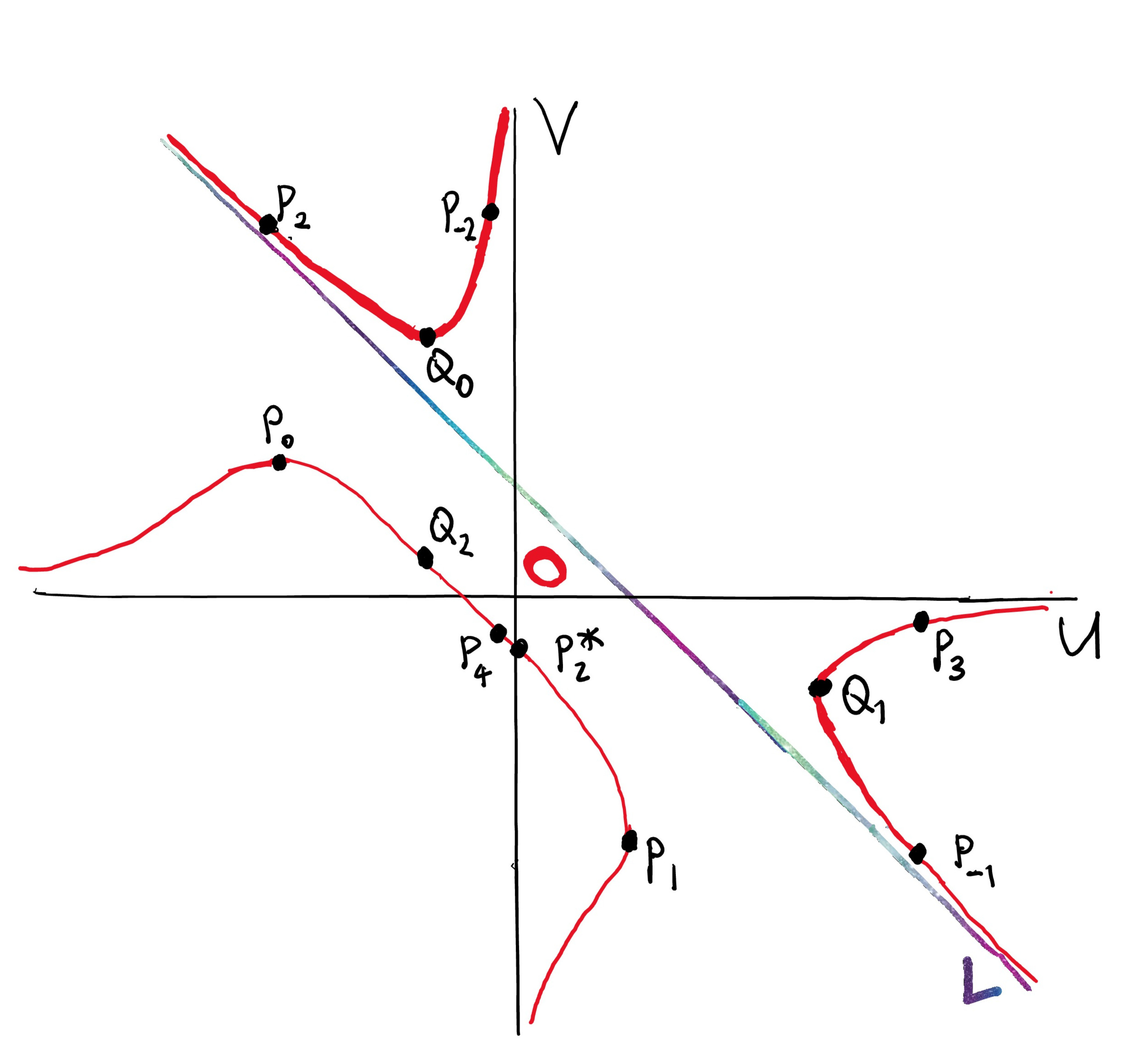
Figure 4: Qualitative sketch of the Somos-5 curve (2.39).

In order to understand how the signs of the quantities (3.5) and (3.6) change with $n$, we need the following result.

Lemma 3.4.

For $n\geq 1$ the signs of the terms in the Somos-5 sequence $(T_{n})$, as in (1.15), repeat in the pattern

$$+-++-+--+--+-+$$ (3.25)

with period 14.

• The periodic sign pattern for the integer sequence (1.15), as above, consists of a block of 7 followed by the same block of 7 but with all the signs reversed, and can be deduced by induction from the signs of the associated sequence of rational numbers $v_{n}$ defined by the right-hand relation in (2.36), which for $n\geq 3$ repeat the pattern

  $$-+-+-+-$$ (3.26)

  with period 7 (cf. Table 5). Indeed, given $T_{1}=-T_{2}=T_{3}=1$, the pattern (3.25) follows from (3.26) by writing $T_{n+1}=v_{n}T_{n}T_{n-1}/T_{n-2}$. So it remains to prove the period 7 sign pattern of the rational sequence $(v_{n})$, which is achieved by considering the corresponding orbit in ${\mathbb{R}}^{2}$ of the QRT map defined by (2.37), that is

  $$\varphi:\,(U,V)\mapsto\big{(}V,U^{-1}(1+V^{-1})\big{)}.$$ (3.27)

  As described above, the orbit lies on the (real) curve (2.39) in the $(U,V)$ plane, shown in Fig.3. The real curve has four connected components, of which only the part in the positive quadrant is compact, but this particular orbit lies outside the positive quadrant, being restricted to the three unbounded components; in contrast, the orbit corresponding to the sequence $(u_{n})$ is given by ratios of the terms of the Somos-5 sequence (1.14), which are all positive, and hence lies on the compact oval. The relevant properties of the orbit corresponding to $(v_{n})$ are not so easy to see from Fig.3, which is drawn to scale, so in Fig.4 we have produced a more schematic drawing of the real curve (2.39) which highlights the essential features. From

  $$\frac{dV}{dU}=-\frac{2UV+V^{2}-5V+1}{U^{2}+2UV-5U+1},$$

  by taking the resultant of the numerator of the above with the equation of the curve we see that the points with horizontal slope have $U$ values given by the four real roots of the quartic $U^{4}+2U^{3}-7U^{2}-2U+7$. In particular, there is a local maximum at the point ${\cal P}_{0}$ with coordinates

  $$\left(-\tfrac{1}{2}\left(\sqrt{2}+1+\sqrt{15+6\sqrt{2}}\right),-\tfrac{1}{2}\left(2\sqrt{2}-5+\sqrt{21-12\sqrt{2}}\right)\right)\approx(-3.63019,0.08211)$$

  and a local minimum at the point ${\cal Q}_{0}$ with coordinates

  $$\left(\tfrac{1}{2}\left(\sqrt{2}-1-\sqrt{15-6\sqrt{2}}\right),\tfrac{1}{2}\left(2\sqrt{2}+5+\sqrt{21+12\sqrt{2}}\right)\right)\approx(-1.06909,6.99523);$$

  the other two stationary points lie on the compact oval. Then we consider the orbit of the map (3.27) starting from the point ${\cal P}^{*}_{3}=(v_{3},v_{4})=(-1,7)$, and it will be convenient to introduce the notation ${\cal P}^{*}_{n}=(v_{n},v_{n+1})$, ${\cal P}_{n}=\varphi^{n}({\cal P}_{0})$ and ${\cal Q}_{n}=\varphi^{n}({\cal Q}_{0})$ for $n\in{\mathbb{Z}}$, as well as letting $\overline{{\cal Q}_{j}{\cal P}_{k}}$ denote the segment of the real curve (2.39) connecting the points ${\cal Q}_{j}$ and ${\cal P}_{k}$, and taking $\overline{{\cal A}{\cal P}_{k}}$ to mean the part of the curve with asymptote ${\cal A}$ starting from the point ${\cal P}_{k}$, where we may have ${\cal A}={\cal U}$ (the $U$ axis), ${\cal V}$ (the $V$ axis) or ${\cal L}$ (the line $U+V=5$). The asymptotes as well as the points ${\cal P}_{0}$, ${\cal Q}_{0}$ and some of their images/preimages under the QRT map are shown in Fig.4. With this notation, for the first 7 iterates we have ${\cal P}_{3}^{*}\in\overline{{\cal Q}_{0}{\cal P}_{-2}}$, ${\cal P}_{4}^{*}\in\overline{{\cal Q}_{1}{\cal P}_{-1}}$, ${\cal P}_{5}^{*}\in\overline{{\cal Q}_{2}{\cal P}_{0}}$, ${\cal P}_{6}^{*}\in\overline{{\cal V}{\cal P}_{1}}$, ${\cal P}_{7}^{*}\in\overline{{\cal L}{\cal P}_{2}}$, ${\cal P}_{8}^{*}\in\overline{{\cal U}{\cal P}_{3}}$, ${\cal P}_{9}^{*}\in\overline{{\cal P}_{2}^{*}{\cal P}_{4}}$, where ${\cal P}_{2}^{*}=(0,-1)$. Under the action of the QRT map $\varphi$, which is given by the composition of the two involutions $\iota_{h}$ and $\iota$ as in (2.40), we have that $\varphi(\overline{{\cal P}_{2}^{*}{\cal P}_{4}})\subset\iota(\overline{{\cal Q}_{1}{\cal P}_{3}})=\overline{{\cal Q}_{0}{\cal P}_{-2}}$, while $\varphi(\overline{{\cal Q}_{0}{\cal P}_{-2}})=\overline{{\cal Q}_{1}{\cal P}_{-1}}$ and $\varphi(\overline{{\cal Q}_{1}{\cal P}_{-1}})=\overline{{\cal Q}_{2}{\cal P}_{0}}$. Also, $\varphi(\overline{{\cal Q}_{2}{\cal P}_{0}})\subset\overline{{\cal V}{\cal P}_{1}}$, $\varphi(\overline{{\cal V}{\cal P}_{1}})=\overline{{\cal L}{\cal P}_{2}}$, $\varphi(\overline{{\cal L}{\cal P}_{2}})=\overline{{\cal U}{\cal P}_{3}}$, and $\varphi(\overline{{\cal U}{\cal P}_{3}})=\overline{{\cal P}_{2}^{*}{\cal P}_{4}}$. Thus it follows by induction that ${\cal P}_{n+3}^{*}\in\overline{{\cal Q}_{0}{\cal P}_{-2}}$, ${\cal P}_{n+4}^{*}\in\overline{{\cal Q}_{1}{\cal P}_{-1}}$, ${\cal P}_{n+5}^{*}\in\overline{{\cal Q}_{2}{\cal P}_{0}}$, ${\cal P}_{n+6}^{*}\in\overline{{\cal V}{\cal P}_{1}}$, ${\cal P}_{n+7}^{*}\in\overline{{\cal L}{\cal P}_{2}}$, ${\cal P}_{n+8}^{*}\in\overline{{\cal U}{\cal P}_{3}}$, ${\cal P}_{n+9}^{*}\in\overline{{\cal P}_{2}^{*}{\cal P}_{4}}$ holds for all $n\geq 0$. The pattern of signs of the coordinates in these 7 consecutive regions is $(-,+)$, $(+,-)$, $(-,+)$, $(+,-)$, $(-,+)$, $(+,-)$, $(-,-)$, which gives the sign pattern (3.26) for the rational sequence $(v_{n})$, as required. ∎

Since $S_{n}>0$ for all $n$, the sign pattern of the sequence $(f_{n})$ is clearly the same as (3.25), consisting of two blocks of 7 that differ by an overall sign, so $\mathrm{sgn}(f_{n+7})=-\mathrm{sgn}(f_{n})$ (where $\mathrm{sgn}$ denotes the sign function). Four of the Schubert parameters with signs are given by monomials in the $f_{n}$ with a homogeneous degree that is even (2 or $-2$), hence their sign pattern repeats with period 7, and the other two have a sign that is determined by the sequence $(v_{n})$, also varying with period 7. As for the signed lengths, their signs are determined by $(T_{n})$, so they each have a pattern that varies with period 14, also made up of two blocks of 7 related by a sign flip. This can be summarized by the following statement.

Corollary 3.5.

The Schubert parameters with signs $(M_{a,n},P_{a,n},X_{a,n})$, $(M_{b,n},P_{b,n},X_{b,n})$ display 5 distinct combinations of signs, which for $n\geq 1$ repeat in a sequence with period 7, beginning with

$$\begin{array}[]{ll}n=1:&(+,+,+),(+,+,+),\\ n=2:&(+,-,+),(-,+,+),\\ n=3:&(-,+,+),(+,+,-),\\ n=4:&(+,-,-),(-,-,+),\\ n=5:&(+,+,+),(+,+,+),\\ n=6:&(+,-,+),(-,+,+),\\ n=7:&(-,+,+),(-,-,+).\end{array}$$ (3.28)

The signed lengths repeat the following sign patterns for $n\geq 1$:

$$\begin{array}[]{ll}\bar{s}_{n}:&+--+-++-++-+--,\\ \bar{a}_{n}:&+++-------++++,\\ \bar{b}_{n}:&++-+--+--+-++-,\\ \bar{c}_{n}:&+-+--+--+-++-+.\end{array}$$ (3.29)

We are now ready to prove most of the statements in Theorem 1.2. For the cases $n\equiv 1$ or $5\,(\bmod\,7)$, both triples of Schubert parameters given by (3.5) and (3.6) are positive and satisfy the constraints, so they produce a Heron triangle with two rational medians and integer sides $(a,b,c)$ whose ratios are given by

$$\frac{a}{c}=\frac{\bar{s}_{n}-\bar{a}_{n}}{\bar{s}_{n}-\bar{c}_{n}}=\frac{\bar{b}_{n}+\bar{c}_{n}}{\bar{a}_{n}+\bar{b}_{n}},\quad\frac{b}{c}=\frac{\bar{s}_{n}-\bar{b}_{n}}{\bar{s}_{n}-\bar{c}_{n}}=\frac{\bar{c}_{n}+\bar{a}_{n}}{\bar{a}_{n}+\bar{b}_{n}},$$

and by (3.29) the signed lengths are either all positive (when $n\equiv 1,12\,(\bmod\,14)$) or all negative (when $n\equiv 5,8\,(\bmod\,14)$), so we can set $a=\pm(\bar{b}_{n}+\bar{c}_{n})$, $b=\pm(\bar{c}_{n}+\bar{a}_{n})$, $c=\pm(\bar{a}_{n}+\bar{b}_{n})$ accordingly, which verifies the formulae (1.19) for the side lengths. Moreover, it follows that the semiperimeter is $s=\pm(\bar{a}_{n}+\bar{b}_{n}+\bar{c}_{n})=\pm\bar{s}_{n}$, and the reduced lengths are $s-a=\pm\bar{a}_{n}$, $s-b=\pm\bar{b}_{n}$, $s-c=\pm\bar{c}_{n}$, so the expression (1.21) for the area follows immediately from Heron’s formula. When $n\equiv 2$ or $6\,(\bmod\,7)$, we need to replace $P_{a}\to-P_{a}^{-1}$ and $M_{b}\to-M_{b}^{-1}$ in order to have two triples of positive coordinates of points on the Schubert surface, but this change of signs is compatible with the two constraints, in the sense that it introduces an overall minus sign on both sides of the first equality in each of (3.3) and (3.4), so that the side ratios of the corresponding Heron triangle with two rational medians are given by

$$\frac{a}{c}=-\frac{\bar{s}_{n}-\bar{a}_{n}}{\bar{s}_{n}-\bar{c}_{n}}=-\frac{\bar{b}_{n}+\bar{c}_{n}}{\bar{a}_{n}+\bar{b}_{n}},\quad\frac{b}{c}=-\frac{\bar{s}_{n}-\bar{b}_{n}}{\bar{s}_{n}-\bar{c}_{n}}=-\frac{\bar{c}_{n}+\bar{a}_{n}}{\bar{a}_{n}+\bar{b}_{n}}.$$

For these values of $n$, from (3.29) we see that $\bar{a}_{n}$ and $\bar{b}_{n}$ are both positive, and $\bar{s}_{n}$ and $\bar{c}_{n}$ are both negative, or vice versa, so we can take integer side lengths $a=\mp(\bar{b}_{n}+\bar{c}_{n})$, $b=\mp(\bar{c}_{n}+\bar{a}_{n})$, $c=\pm(\bar{a}_{n}+\bar{b}_{n})$, which verifies (1.19), while in this case the semiperimeter and reduced lengths are permutations (up to sign) of the signed lengths, as (depending on the value of $n\bmod 14$) we have $s=\mp\bar{c}_{n}$, $s-a=\pm\bar{b}_{n}$, $s-b=\pm\bar{a}_{n}$, $s-c=\mp\bar{s}_{n}$, which confirms the area formula (1.21). The analysis of the other three combinations of signs in (3.28) proceeds similarly. For the case of $n\equiv 3\,(\bmod\,7)$ only the second constraint (3.4) acquires an overall minus sign when the negative Schubert parameters $M_{a},X_{b}$ are replaced by $-M_{a}^{-1},-X_{b}^{-1}$, and we find $s=\mp\bar{b}_{n}$, $s-a=\pm\bar{c}_{n}$, $s-b=\mp\bar{s}_{n}$, $s-c=\pm\bar{a}_{n}$ (according to whether $n\equiv 3$ or $10\,(\bmod\,14)$). When $n\equiv 4\,(\bmod\,7)$, the replacements $P_{a}\to-P_{a}^{-1}$, $X_{a}\to-X_{a}^{-1}$, $M_{b}\to-M_{b}^{-1}$, $P_{b}\to-P_{b}^{-1}$ result in an overall change of sign in the second constraint only, as the signs in (3.28) and (3.29) are the exact opposite of those in the previous case, so we have $s=\pm\bar{b}_{n}$, $s-a=\mp\bar{c}_{n}$, $s-b=\pm\bar{s}_{n}$, $s-c=\mp\bar{a}_{n}$. Finally, when $n\equiv 0\,(\bmod\,7)$, replacing $M_{a}\to-M_{a}^{-1}$, $M_{b}\to-M_{b}^{-1}$, $P_{b}\to-P_{b}^{-1}$ again only introduces a minus sign in the second constraint, and we also find $s=\pm\bar{b}_{n}$, $s-a=\mp\bar{c}_{n}$, $s-b=\pm\bar{s}_{n}$, $s-c=\mp\bar{a}_{n}$ in this case. Thus in each case we have a pair of positive triples of Schubert parameters satisfying the necessary constraints. If we further require that these should correspond to the half-angle cotangents of appropriate angles in the triangle (cf. Fig.1), then it may be necessary to apply one or both of the transformations

$$(M_{a},P_{a},X_{a})\to(M_{a}^{-1},P_{a}^{-1},X_{a}^{-1}),\qquad(M_{b},P_{b},X_{b})\to(M_{b}^{-1},P_{b}^{-1},X_{b}^{-1}),$$ (3.30)

in order to satisfy the conditions (1.9).

Having shown that the Schubert parameters with signs in the main sequence for $n\geq 1$ can be consistently transformed to a set of positive Schubert parameters, thus providing a sequence of Heron triangles with two rational medians $k,\ell$, whose integer sides $(a,b,c)$ and area $\Delta$ are given by the formulae in Theorem 1.2, it remains to verify the expressions (1.20) for the medians, and also show that $\gcd(a,b,c)=1$, which requires a bit more work. We begin by defining signed median lengths, given by

$$\bar{k}_{n}=\frac{1}{2}S_{n+4}T_{n+4}(T_{n}T_{n+1}^{2}T_{n+2}-S_{n}S_{n+1}^{2}S_{n+2}),\qquad\bar{\ell}_{n}=\frac{1}{2}S_{n}T_{n}(S_{n+2}S_{n+3}^{2}S_{n+4}-T_{n+2}T_{n+3}^{2}T_{n+4}),$$ (3.31)

where the overall signs have been chosen so that these initially coincide with the positive median lengths, i.e. when $n=1$ we have $k=\bar{k}_{1}=35/2$, $\ell=\bar{\ell}_{1}=97/2$. In order to show that these quantities agree with the median lengths up to a sign, we need to prove that $\bar{k}_{n}$ satisfies a signed version of one of the identities in (1.6), and that $\bar{\ell}_{n}$ satisfies a signed version of one of the analogous identities for $\ell$, obtained by replacing $a\to b$, $b\to c$, $c\to a$ and $k\to\ell$ on the right-hand side of each formula. We start by picking the middle identity for $P=P_{a}$, which becomes

$$P_{a,n}=\frac{4\Delta_{n}}{4(\bar{s}_{n}-\bar{c}_{n})\bar{k}_{n}+(\bar{s}_{n}-\bar{a}_{n})^{2}-(\bar{s}_{n}-\bar{b}_{n})^{2}-3(\bar{s}_{n}-\bar{c}_{n})^{2}},$$ (3.32)

obtained by setting $P_{a}\to P_{a,n}$ on the left-hand side, and replacing $a,b,c$ and $k$ by their signed versions on the right-hand side, as well as inserting the signed area

$$\Delta_{n}=S_{n}S_{n+1}S_{n+2}^{2}S_{n+3}S_{n+4}T_{n}T_{n+1}T_{n+2}^{2}T_{n+3}T_{n+4}$$

in the numerator. As for $\ell$, the direct analogue of the first identity in (1.6) is

$$M_{b}=\frac{4\Delta}{4c\ell+b^{2}-3c^{2}-a^{2}},$$

but instead, for reasons that will shortly become clear, we would like to use another expression for $M_{b}$, namely

$$M_{b}=\frac{4c\ell-b^{2}+3c^{2}+a^{2}}{4\Delta},$$

where the latter is seen to be equivalent to the former due to the relation $16\Delta^{2}=16c^{2}\ell^{2}-(b^{2}-3c^{2}-a^{2})^{2}$, which follows from Heron’s formula and the expression for $\ell^{2}$ in (1.3). So as the signed analogue of the latter identity for $M_{b}$, we take

$$M_{b,n}=\frac{4(\bar{s}_{n}-\bar{c}_{n})\bar{\ell}_{n}-(\bar{s}_{n}-\bar{b}_{n})^{2}+3(\bar{s}_{n}-\bar{c}_{n})^{2}+(\bar{s}_{n}-\bar{a}_{n})^{2}}{4\Delta_{n}}.$$ (3.33)

Lemma 3.6.

The signed median lengths $\bar{k}_{n}$, $\bar{\ell}_{n}$ given by (3.31) satisfy the relations (3.32) and (3.33) for all $n\in{\mathbb{Z}}$.

• To begin with, we rewrite (3.32) as

  $$P_{a,n}^{-1}=\frac{4(\bar{s}_{n}-\bar{c}_{n})\bar{k}_{n}+(\bar{s}_{n}-\bar{a}_{n})^{2}-(\bar{s}_{n}-\bar{b}_{n})^{2}-3(\bar{s}_{n}-\bar{c}_{n})^{2}}{4\Delta_{n}},$$ (3.34)

  and consider the symmetry $n\to-n-4$, as in Lemma 3.2. On the left-hand side we have $P_{a,-n-4}^{-1}=-M_{b,n}$, while on the right we use the transformations (3.13) together with the linear relation (3.8), as well as $\bar{k}_{-n-4}=\bar{\ell}_{n}$ and $\Delta_{-n-4}=\Delta_{n}$, to see that (up to an overall minus sign on both sides), the relation (3.34) is transformed to (3.33). Therefore it will be sufficient to prove the above relation involving $\bar{k}_{n}$ alone, and we can proceed as in the proofs of Lemma 3.1 and Theorem 3.3, by substituting in the analytic formulae for each of the terms and regarding it as an identity between elliptic functions of $z=(n+2){\kappa}$, so that the left-hand side has simple poles at the places $z\equiv 0,{\omega},{\kappa},{\kappa}+{\omega}\bmod\Lambda$. However, we also wish to exploit the additional symmetry under shifting by the half-period ${\omega}$, as we have $P_{a,n}\to P_{a,n}$ under this symmetry, and using the results of our previous calculations we see that overall the right-hand side of (3.34) is also left invariant by this transformation. Thus it is sufficient to check only the poles at $z=0,{\kappa}$ as well as one other value where the relation is finite, and the case $n=1$ (corresponding to $z=3{\kappa}$) where $P_{a,1}=2/3$ is readily verified. Then since we only have residues at two simple poles to check, corresponding to the values $n=-2,-1$, we can use the simplified method with a local parameter ${\epsilon}$, as at the end of the proof of Theorem 3.3. Using (3.5) and (3.8) we can rewrite (3.34) as

  $$-u_{n+2}v_{n+2}=\frac{4\left(1+\frac{\bar{b}_{n}}{\bar{a}_{n}}\right)\frac{\bar{k}_{n}}{\bar{a}_{n}}+\left(\frac{\bar{s}_{n}}{\bar{a}_{n}}-1\right)^{2}-\left(1+\frac{\bar{c}_{n}}{\bar{a}_{n}}\right)^{2}-3\left(1+\frac{\bar{b}_{n}}{\bar{a}_{n}}\right)^{2}}{4{\Delta_{n}}/{\bar{a}_{n}^{2}}}.$$ (3.35)

  On the right-hand side above we can make use of the expressions (3.24), as well as

  $$\bar{c}_{n}/\bar{a}_{n}=-f_{n}^{2}f_{n+1}v_{n+2}^{2}v_{n+3}^{2}/f_{n+2}$$

  and

  $$\frac{\bar{k}_{n}}{\bar{a}_{n}}=-\frac{f_{n+4}v_{n+2}v_{n+3}^{2}(1-f_{n}f_{n+1}^{2}f_{n+2})}{2f_{n+2}},\qquad\frac{\Delta_{n}}{\bar{a}_{n}^{2}}=f_{n}f_{n+1}f_{n+3}f_{n+4}v_{n+2}^{2}v_{n+3}^{2}.$$

  Now when $n=-2$, at leading order on the left-hand side we have $-u_{0}v_{0}\sim{\epsilon}^{-1}$, while on the right-hand side the leading order in the denominator is $4\Delta_{-2}/\bar{a}_{-2}^{2}\sim 4{\epsilon}^{-4}$. In the numerator, $\bar{b}_{-2}/\bar{a}_{-2}\sim{\epsilon}^{2}$ and $\bar{k}_{-2}/\bar{a}_{-2}\sim\frac{1}{2}{\epsilon}^{-3}$, hence the first term gives the leading order contribution $4(1+\bar{b}_{-2}/\bar{a}_{-2})\bar{k}_{-2}/\bar{a}_{-2}\sim 2{\epsilon}^{-5}$, but for the difference of squares that follows we need a correction at next-to-leading order, so that from $\bar{s}_{-2}/\bar{a}_{-2}={\epsilon}^{-3}+\frac{1}{2}{\epsilon}^{-2}+\cdots$, $\bar{c}_{-2}/\bar{a}_{-2}={\epsilon}^{-3}-\frac{1}{2}{\epsilon}^{-2}+\cdots$ we find $(\bar{s}_{-2}/\bar{a}_{-2}-1)^{2}-(\bar{c}_{-2}/\bar{a}_{-2}+1)^{2}\sim 2{\epsilon}^{-5}$, and the final term $-3(1+\bar{b}_{-2}/\bar{a}_{-2})^{2}$ gives a lower order contribution at $O({\epsilon}^{-4})$; thus overall at leading order the right-hand side gives $(2{\epsilon}^{-5}+2{\epsilon}^{-5})/(4{\epsilon}^{-4})={\epsilon}^{-1}$, as required. When $n=-2$, the left-hand side is $-u_{1}v_{1}\sim-{\epsilon}^{-1}$, while the denominator of the right-hand side is $\Delta_{-1}/\bar{a}_{-1}^{2}\sim 8{\epsilon}^{-1}$, and the numerator contains the terms $\bar{b}_{-1}/\bar{a}_{-1}\sim{\epsilon}^{-1}$, $\bar{k}_{-1}/\bar{a}_{-1}\sim-{\epsilon}^{-1}$, $\bar{s}_{-1}/\bar{a}_{-1}\sim-4$, $\bar{c}_{-1}/\bar{a}_{-1}\sim-{\epsilon}^{-1}$, so that overall these combine to give $(-4{\epsilon}^{-2}-{\epsilon}^{-2}-3{\epsilon}^{-2})/(8{\epsilon}^{-1})=-{\epsilon}^{-1}$ at leading order, in agreement with the left-hand side. Note also that for the values $n=-4,-3$ and $0$, the left-hand side is finite while the other side has removable singularities: some of the terms in the numerator/denominator on the right-hand side of (3.35) are singular, but overall these cancel to give a finite value in the limit ${\epsilon}\to 0$; so the relation holds as an identity between elliptic functions of $z=(n+2){\kappa}$, and in particular for all $n\in{\mathbb{Z}}$. ∎

Given that $\bar{k}_{n}$ satisfies (3.32), for each $n$ we can compare this with the corresponding positive Schubert parameter $P_{a}>0$, given by

$$P_{a}=\frac{4\Delta}{4ck+a^{2}-b^{2}-3c^{2}}=\frac{4ck-a^{2}+b^{2}+3c^{2}}{4\Delta},$$

where we use either the first or the second rational expression above involving $a,b,c,k$ and $\Delta$, according to whether $P_{a,n}=\pm P_{a}^{\pm 1}$, determined by $n\bmod 7$ as in Corollary 3.5. Now $\mathrm{sgn}(\Delta_{n})=\mathrm{sgn}(T_{n}T_{n+1}T_{n+3}T_{n+4})$, which repeats the pattern

$$\Delta_{n}:\qquad++--+++$$

with period 7, while our previous analysis also showed that, for each $n$, $\bar{s}_{n}-\bar{c}_{n}=\mathrm{sgn}(\bar{s}_{n}-\bar{c}_{n})\,c$, where the sign pattern is

$$\bar{s}_{n}-\bar{c}_{n}:\qquad++-+--+--+-++-$$

with period 14. For the cases $n\equiv 1,2,5,6,0\,(\bmod\,7)$ we see that $\Delta_{n}=\Delta$, and then according to whether $P_{a,n}>0$ (when $n\equiv 1,5,0$) or $P_{a,n}<0$ (when $n\equiv 2,6$) we can directly compare the right-hand side of (3.32) with either the first formula for $P_{a}$ above, or compare $-P_{a,n}^{-1}$ with the second formula above, respectively; then since the squared terms can always be identified, that is $a^{2}=(\bar{s}_{n}-\bar{a}_{n})^{2}$ etc., we have $ck=(\bar{s}_{n}-\bar{c}_{n})\bar{k}_{n}$ in the first case, giving $\bar{k}_{n}=\mathrm{sgn}(\bar{s}_{n}-\bar{c}_{n})\,k$, but $ck=-(\bar{s}_{n}-\bar{c}_{n})\bar{k}_{n}$ in the second case, giving $\bar{k}_{n}=-\mathrm{sgn}(\bar{s}_{n}-\bar{c}_{n})\,k$. However, the cases $n\equiv 3,4\,(\bmod\,7)$, when $\Delta_{n}=-\Delta$, are different because in those cases we need to apply the first of the transformations in (3.30) to ensure that (1.9) holds. So for $n\equiv 3\,(\bmod\,7)$ that means comparing $P_{a,n}^{-1}$ with the second formula for $P_{a}$ above, yielding $\bar{k}_{n}=-\mathrm{sgn}(\bar{s}_{n}-\bar{c}_{n})\,k$, and for $n\equiv 4\,(\bmod\,7)$ it requires that $-P_{a,n}$ should be compared with the first formula for $P_{a}$, hence $\bar{k}_{n}=\mathrm{sgn}(\bar{s}_{n}-\bar{c}_{n})\,k$. Thus overall we see that $\bar{k}_{n}$ is related to the median length $k$ by an overall sign, which varies with period 14 in the following pattern:

$$\bar{k}_{n}:\qquad+-++-++-+--+--.$$ (3.36)

Similarly, $\bar{\ell}_{n}$ is equal to the median length $\ell$ up to a sign with pattern

$$\bar{\ell}_{n}:\qquad+-++-+--+--+-+,$$ (3.37)

and this verifies that the formulae (1.20) hold.

Based on computer experiments, it was observed in [7] that for the triangles in the main sequence, the pairs $(\theta,\phi)$ corresponding to the parametrization (1.10), given by (1.11) with $+$ signs in both equations, cycle through one of five isomorphic plane curves in a pattern that repeats with period 7. Applying the symmetry $a\leftrightarrow b$, $k\leftrightarrow\ell$, one obtains an alternative pair of parameters

$$\tilde{\theta}=\frac{c-b+2k}{2s},\qquad\tilde{\phi}=\frac{a-c+2\ell}{2s},$$ (3.38)

and Buchholz and Rathbun noted that these pairs cycle with period 7 through the same set of curves but in a different order, namely ${\cal C}_{1},{\cal C}_{2},{\cal C}_{3},{\cal C}_{4},{\cal C}_{1},{\cal C}_{2},{\cal C}_{5}$. A more detailed study of the allowed discrete symmetries in [9] showed that by applying appropriate permutations of $a,b,c,k,\ell$ and changes of sign, one could also obtain pairs of coordinates on three more (isomorphic) curves ${\cal C}_{6},{\cal C}_{7},{\cal C}_{8}$. However, until now there was no explanation for the period 7 behaviour with respect to the index $n$ in the main sequence, which we provide here.

Theorem 3.7.

For $n\geq 1$, the rational parameters

$$\theta=\frac{c-a+2\ell}{a+b+c},\qquad\phi=\frac{b-c+2k}{a+b+c}$$

corresponding to the main sequence of Heron triangles with sides $(a,b,c)$ and medians $k,\ell$ lie on one of five birationally equivalent plane curves of genus one, which repeat in a pattern with period 7. The same is true for any such sequence of parameters obtained from these by the action of the discrete symmetry group that leaves the equations $4k^{2}=2b^{2}+2c^{2}-a^{2}$, $4\ell^{2}=2c^{2}+2a^{2}-b^{2}$ invariant.

• We begin by considering the pair of quantities

  $$\theta_{n}=\frac{\bar{a}_{n}-\bar{c}_{n}+2\bar{\ell}_{n}}{2\bar{s}_{n}},\qquad\phi_{n}=\frac{\bar{c}_{n}-\bar{b}_{n}+2\bar{k}_{n}}{2\bar{s}_{n}},$$

  obtained by replacing $a,b,c,k,\ell$ by their signed counterparts $\bar{s}_{n}-\bar{a}_{n},\bar{s}_{n}-\bar{b}_{n},\ldots$ etc. For $n=1$ this coincides with $\theta,\phi$. Moreover, from the analytic parametrization of the two Somos-5 sequences, this gives a pair of independent elliptic functions of $z=(n+2){\kappa}$. Then by a standard result in the theory of elliptic functions, the pairs $(\theta_{n},\phi_{n})$ lie on a plane curve ${\cal C}$ of genus one, which is birationally equivalent to the original elliptic curve (this follows from the Riemann-Roch theorem, but there is also an explicit classical method for constructing the equation of ${\cal C}$, based on the expressions for $\theta_{n},\phi_{n}$ in terms of $\wp,\wp^{\prime}$ [2]). Under the change $n\to n+1$, the original pair $(\theta,\phi)$ corresponds to a different pair of elliptic functions, because each term $a,b,\ldots$ that appears is related to $\bar{s}_{n}-\bar{a}_{n},\bar{s}_{n}-\bar{b}_{n},\ldots$ by a sign which changes with $n$; so the pair of coordinates for the next value of $n$ will lie on a different curve, ${\cal C}^{*}$ say. Now all of these signs repeat with period 14, but in each block of 7 the signs are flipped with respect to the previous block, and only the ratio of terms appears in $\theta,\phi$, so their overall pattern of signs repeats with period 7, hence there are at most 7 different curves repeating with this period. However, a closer examination of (3.29), (3.36) and (3.37) reveals that there are really only 5 different pairs of functions appearing in each block of 7, because all the signs for $n\equiv 1\,(\bmod\,7)$ and $n\equiv 5\,(\bmod\,7)$ are the opposite of each other, and similarly for $n\equiv 2\,(\bmod\,7)$ and $n\equiv 6\,(\bmod\,7)$. The same argument applies to any pair $(\theta,\phi)$ obtained from this one by the action of the discrete symmetry group. ∎

In order to show that the side lengths given by (1.19) have greatest common divisor 1 for all $n\geq 1$, it is necessary to reconsider the orbits of the QRT map $\varphi$ defined by (3.27), associated with the rational sequences $(u_{n})$, $(v_{n})$, and examine their reduction modulo a prime $p$, which corresponds to considering the map over the finite field ${\mathbb{F}}_{p}$. (For a detailed treatment of QRT maps over finite fields, see [33].) A general QRT map (over any field) is a birational map $\varphi:\,{\mathbb{P}}^{1}\times{\mathbb{P}}^{1}\to{\mathbb{P}}^{1}\times{\mathbb{P}}^{1}$ given by a composition of two involutions, and as already mentioned, each orbit lies on a curve belonging to a pencil of biquadratic curves in the plane; generic curves ${\cal C}$ have genus one, and the orbit gives a sequence of points $\hat{{\cal P}}_{0}+n{\cal P}\in{\cal C}$, with each iteration of $\varphi$ corresponding to addition of the point ${\cal P}$ in the group law of the curve. For the particular case at hand, the curve is given by (2.39), which has identity element ${\cal O}=(\infty,\infty)$, and $\iota$ in (2.40) is the elliptic involution that sends any point $\hat{\cal P}\to-\hat{\cal P}$. Under the QRT map $\varphi=\iota\circ\iota_{h}$, ${\cal P}=(\infty,0)$ is the point being added at each step, and the orbit corresponding to the Somos-5 sequence (1.14) via (2.36) is

$$\varphi^{n}(u_{0},u_{1})=(u_{n},u_{n+1})=(1,1)+n{\cal P},$$ (3.39)

where the initial point $\hat{{\cal P}}_{0}=(u_{0},u_{1})=(1,1)\in{\cal C}$ is 2-torsion, while the orbit associated with the other sequence (1.15) is

$$\varphi^{n}(v_{0},v_{1})=(v_{n},v_{n+1})=n{\cal P},$$ (3.40)

with initial point ${\cal O}=(v_{0},v_{1})=(\infty,\infty)$.

The above description is valid over ${\mathbb{C}}$ or any subfield where the orbit is defined, in particular over ${\mathbb{Q}}$, in which case ${\cal P}$ is an infinite order element in the Mordell-Weil group of the curve ${\cal C}({\mathbb{Q}})$, which is generated by ${\cal P}$ and the 2-torsion point $\hat{{\cal P}}_{0}=(1,1)$. Under reduction $\bmod\,p$ the same description holds provided that $p$ is a prime of good reduction, so that the curve ${\cal C}({\mathbb{F}}_{p})$ is non-singular, with the main difference being that now the curve has finitely many points satisfying the Hasse-Weil bound $\left|p+1-\#{\cal C}({\mathbb{F}}_{p})\right|\leq 2\sqrt{p}$, so ${\cal P}$ has some finite order which we denote by $\mathrm{ord}_{p}({\cal P})$. Hence it follows that both orbits (3.39) and (3.40) over ${\mathbb{F}}_{p}$ are periodic with the same period $\mathrm{ord}_{p}({\cal P})$.

For primes of bad reduction, which in this case are 2,3 and 17, the situation is slightly more complicated. For the primes $p=2,3$, we find that the singular curve ${\cal C}({\mathbb{F}}_{p})$ is reducible, since $-5\bmod 2=-5\bmod 3=1$, so in both cases we can factorize (2.39) as

$$(UV+1)(U+V+1)=0.$$ (3.41)

When $p=2$, the two orbits $(u_{n},u_{n+1})$ and $(v_{n},v_{n+1})$ are the same up to a shift of starting point, repeating the sequence

$$(\infty,\infty),(\infty,0),(0,1),(1,1),(1,0),(0,\infty)$$

with period $6=2\times(2+1)$, corresponding to the fact that each (genus zero) irreducible component of (3.41) is isomorphic to ${\mathbb{P}}^{1}({\mathbb{F}}_{2})$, so contains 3 points, and the orbit alternates between points on each component, i.e. $(\infty,0),(1,1),(0,\infty)\in\{\,UV+1=0\,\}$ and $(\infty,\infty),(0,1),(1,0)\in\{\,U+V+1=0\,\}$. Similarly, when $p=3$ both orbits have period $8=2\times(3+1)$, repeating the sequence

$$(\infty,\infty),(\infty,0),(0,2),(2,1),(1,1),(1,2),(2,0),(0,\infty),$$

which again alternates between the two irreducible components of the curve (3.41). For $p=17$, the curve (2.39) is irreducible and singular: this is a case of non-split multiplicative reduction [39], so it has genus zero and contains $\#{\cal C}({\mathbb{F}}_{17})=p+2=19$ points, and after removing the singular point $(5,5)$, ${\cal C}({\mathbb{F}}_{17})\setminus\{\,(5,5)\,\}$ has the structure of an abelian group of order 18. The two orbits both have period 9, corresponding to the two cosets of the cyclic subgroup of order 9 generated by ${\cal P}$; the coordinates of the points in these two orbits can be read off from Table 7, which also includes part of the associated periodic sequence $(f_{n}\bmod\,17)$ (of period 18).

Although it is not essential to our main argument, we can now offer a brief explanation for how the periods modulo a prime arise for the corresponding Somos-5 sequences. Setting $t=\mathrm{ord}_{p}({\cal P})$ and working $\bmod\,p$, from the relation $u_{n+t}=u_{n}$ we have

$$\frac{S_{n-2+t}S_{n+1+t}}{S_{n-1+t}S_{n+t}}=\frac{S_{n-2}S_{n+1}}{S_{n-1}S_{n}}$$

for all $n$, and clearly the period of the Somos-5 sequence must be a multiple of $t$. (We will write everything for the sequence $(S_{n})$, but the same treatment applies to $(T_{n})$ or any other Somos-5 sequence.) Somos-5 sequences have a 3-parameter group of gauge transformations which leave the ratios $u_{n}$, and hence the recurrence (1.16), unchanged: one can replace $S_{n}\to A^{*}_{\pm}(B^{*})^{n}\,S_{n}$, i.e. rescale all even/odd index terms by an arbitrary non-zero scalar $A^{*}_{\pm}$, and rescale each term by the powers of another arbitrary quantity $B^{*}\neq 0$; this symmetry group has a natural interpretation in terms of the quiver that defines the associated cluster algebra [21]. Hence we see that $S_{n}$ and $S_{n+t}$ should be related by a gauge transformation of this kind.

Proposition 3.8.

Under shifting by $t=\mathrm{per}(u_{n}\bmod\,p)$, the period of the associated QRT map, the Somos-5 sequence reduced $\bmod\,p$ satisfies

$$S_{n+t}=A^{*}_{\pm}(B^{*})^{n}\,S_{n},\qquad A^{*}_{+},A^{*}_{-}B^{*},(B^{*})^{2}\in{\mathbb{F}}_{p}^{*}$$ (3.42)

for even/odd $n$, respectively, where $A^{*}_{+},A^{*}_{-},B^{*}$ are constants independent of $n$.

• To prove this gauge transformation formula directly, define the ratio $r_{n}=S_{n+t}/S_{n}$, and observe that $u_{n+t}=u_{n}$ for all $n$ implies that $r_{n+2}/r_{n}=r_{n+3}/r_{n+1}=r_{n+4}/r_{n+2}=r_{n+5}/r_{n+3}=(B^{*})^{2}$ say, a constant in ${\mathbb{F}}_{p}^{*}$ independent of $n$, and this can be solved separately for even/odd $n$ to give $r_{n}=A^{*}_{\pm}(B^{*})^{n}$, where $A^{*}_{+}=r_{0}$, $A^{*}_{-}B^{*}=r_{1}\in{\mathbb{F}}_{p}^{*}$ (assuming none of the terms in these ratios is zero). ∎

Corollary 3.9.

Let $t$ be the order of the point ${\cal P}\in{\cal C}({\mathbb{F}}_{p})$ if $p$ is a prime of good reduction (or equivalently, the period of $(u_{n}\bmod\,p)$, appropriately reinterpreted in the case of bad reduction). Then the period of the Somos-5 sequence $\bmod\,p$ is a multiple of $t$, given by

$$\mathrm{per}(S_{n}\bmod\,p)=\ell^{*}\,t\leq 2(p-1)t,$$ (3.43)

where (up to a possible factor of 2) $\ell^{*}$ denotes the lowest common multiple of $\mathrm{ord}_{p}\big{(}(B^{*})^{2}\big{)}$ and/or the orders in ${\mathbb{F}}_{p}^{*}$ of one or two other combinations of $A^{*}_{+},A^{*}_{-},B^{*}$, depending on the parity of $t$.

• Iterating the quasiperiodicity relation (3.42) $j$ times when $t$ is even yields

  $$S_{n+jt}=(A^{*}_{\pm})^{j}(B^{*})^{nj+tj(j-1)/2}\,S_{n},$$

  for even/odd $n$, so requiring $S_{n+jt}=S_{n}$ for all $n$ imposes the conditions

  $$(B^{*})^{2j}=1,\qquad(A_{+}^{*})^{j}=(A_{-}^{*}B^{*})^{j}=(B^{*})^{-tj(j-1)/2}=\pm 1,$$ (3.44)

  where the choice of $j$ satisfying the first condition for a given $B^{*}$ fixes the sign on the right. Then $\ell^{*}$ is the smallest positive value of $j$ that satisfies all these conditions. An odd value of $\ell^{*}$ is only possible in the case that $(B^{*})^{2}$, $A_{+}^{*}$ and $A_{-}^{*}B^{*}$ are all quadratic non-residues in ${\mathbb{F}}_{p}^{*}$, in which case only the plus sign can occur on the right-hand side above, and

  $$\ell^{*}=\mathrm{lcm}\big{(}\mathrm{ord}_{p}(A^{*}_{+}),\mathrm{ord}_{p}(A^{*}_{-}B^{*}),\mathrm{ord}_{p}((B^{*})^{2})\big{)},$$

  but otherwise there must be an even $\ell^{*}|\mathrm{lcm}\big{(}\mathrm{ord}_{p}(A^{*}_{+}),\mathrm{ord}_{p}(A^{*}_{-}B^{*}),\mathrm{ord}_{p}((B^{*})^{2})\big{)}$, where it may be possible to divide out some factors of 2 from the first two terms, depending on the orders of these elements. For odd $t$, iterating (3.42) $j$ times produces

  $$S_{n+jt}=(A^{*}_{\pm})^{\left\lfloor\frac{j+1}{2}\right\rfloor}(A^{*}_{\mp})^{\left\lfloor\frac{j}{2}\right\rfloor}(B^{*})^{nj+tj(j-1)/2}\,S_{n},$$

  and then by requiring $S_{n+jt}=S_{n}$ for all $n$, in the case of odd $j$ (exploiting the freedom to replace $B^{*}\to-B^{*}$ and $A^{*}_{-}\to-A^{*}_{-}$ simultaneously) this leads to

  $$A^{*}_{+}=A^{*}_{-},\qquad(B^{*})^{j}=(A^{*}_{+})^{j}=1\implies\ell^{*}=\mathrm{lcm}\big{(}\mathrm{ord}_{p}(A^{*}_{+}),\mathrm{ord}_{p}(B^{*})\big{)},$$

  corresponding to a situation where $\tilde{K}_{0}=\tilde{K}_{1}$ and all the terms satisfy the same Somos-4 recurrence (cf. equation (2.5) and [44]). For an even value of $j$ with $t$ odd, we find instead

  $$(B^{*})^{j}=1,\qquad(A^{*}_{+}A^{*}_{-}B^{*})^{j/2}=(B^{*})^{\big{(}1-t(j-1)\big{)}j/2}=1,$$

  so now, given the values of $(B^{*})^{2}$ and $A^{*}_{+}A^{*}_{-}B^{*}$, the smallest possible value of $j/2$ can be found, yielding

  $$\ell^{*}=2\,\mathrm{lcm}\big{(}\mathrm{ord}_{p}(A^{*}_{+}A^{*}_{-}B^{*}),\mathrm{ord}_{p}((B^{*})^{2})\big{)}.$$ (3.45)

  The upper bound on the period comes from Fermat’s little theorem. ∎

An advantage of the relation (3.42) is that it allows the period of the Somos-5 sequence to be computed from (3.43) without calculating so many terms: in general it is sufficient to find the minimum $t$ such that $(u_{0},u_{1})=(u_{t},u_{t+1})$, giving $t=\mathrm{ord}_{p}({\cal P})$, which requires the $t+5$ adjacent terms $S_{-2},\ldots,S_{t+2}$, and then $A^{*}_{\pm},B^{*}$ can be obtained from the ratios $S_{t}/S_{0}$, $S_{t+1}/S_{1}$ and $S_{t+2}/S_{2}$ (provided $S_{0}S_{1}S_{2}\neq 0$, otherwise one of the ratios $S_{t-1}/S_{-1}$, $S_{t-2}/S_{-2}$ can be used instead). For example, in the case of the sequence (1.14) taken $\bmod\,23$, we find that $(u_{n}\bmod\,23)$ repeats the pattern $1,1,2,13,20,3,20,13,2$ with period 9, so $t=\mathrm{ord}_{23}({\cal P})=9$ which is odd, while $A^{*}_{+}\equiv S_{9}/S_{0}\bmod\,23=S_{10}/S_{1}\bmod\,23=21$ and $S_{11}/S_{2}\bmod\,23=20$, thus we find $(B^{*})^{2}=20/21=13=6^{2}$ in ${\mathbb{F}}_{23}$, and taking $B^{*}=6$ gives $A^{*}_{-}=21/6=15\neq A^{*}_{+}$; then $\mathrm{ord}_{23}(13)=11$ and $\mathrm{ord}_{23}(21\times 15\times 6)=\mathrm{ord}_{23}(21^{2})=11$, so $\ell^{*}=22$ by (3.45), hence $\mathrm{per}(S_{n}\bmod\,23)=9\times 22=198$, in agreement with the value found by Robinson in [47]. As another example, for the sequence (1.15) taken $\bmod\,61$, the corresponding terms $(v_{n}\bmod\,61)$ have a repeating pattern

$$\infty,\infty,0,60,7,25,12,34,11,32,2,1,1,2,32,11,34,12,25,7,60,0$$

with even period $t=22$, and from the terms $1,1$ in the middle it is apparent that this is the same as the orbit $(u_{n}\bmod\,61)$ but shifted; thus from $T_{21}/T_{-1}\bmod\,61=14\equiv A_{-}^{*}(B^{*})^{-1}$, $T_{23}/T_{1}\bmod\,61=60\equiv A_{-}^{*}B^{*}$, $T_{24}/T_{2}\bmod\,61=14\equiv A_{+}^{*}(B^{*})^{2}$ we find $A_{-}^{*}=13=14^{2}$, $A_{+}^{*}=48=14^{-1}$, $B^{*}=14$ in ${\mathbb{F}}_{61}$, and $\mathrm{ord}_{61}(14)=6$, so $\ell^{*}$ divides $\mathrm{lcm}\big{(}\mathrm{ord}_{61}(14^{-1}),\mathrm{ord}_{61}(14^{3}),\mathrm{ord}_{61}(14^{2})\big{)}$=6, the smallest value of $j$ satisfying all the requirements in (3.44), hence the period of the sequence $(T_{n}\bmod\,61)$ is $22\times 6=132$, and this is the same as the period of the original Somos-5 sequence $(S_{n}\bmod\,61)$ as found in [47].

We are now ready to finish off the proof of the main theorem.

Lemma 3.10.

For all $n\in{\mathbb{Z}}$, the terms of the sequences (1.14) and (1.15) with the same index are coprime, that is

$$\gcd(S_{n},T_{n})=1.$$

• Suppose that for some $n$ the terms $S_{n}$ and $T_{n}$ have a common divisor. Then for the reduced sequences in ${\mathbb{F}}_{p}$ it follows that $S_{n}\equiv 0\equiv T_{n}$, and so $u_{n}=u_{n+1}=\infty=v_{n}=v_{n+1}$. If $p$ is a prime of good reduction for the curve ${\cal C}$ given by (2.39), then in the group law of ${\cal C}({\mathbb{F}}_{p})$ this implies that $(1,1)+n{\cal P}={\cal O}=n{\cal P}$, which is a contradiction. If $p$ is a prime of bad reduction, then we have $p=2,3$ or 17, and $p=2$ or $p=3$ are impossible by Proposition 2.17, while Table 7 shows that 17 is never a divisor of $S_{n}$, since the sequence $(u_{n}\bmod\,17)$ has period 9 and remains finite. ∎

Table 7: The analogue of Table 5 in the finite field ${\mathbb{F}}_{17}$.

$n$	0	1	2	3	4	5	6	7	8	9
$u_{n}$	$1$	$1$	$2$	$10$	$15$	$6$	$15$	$10$	$2$	$1$
$v_{n}$	$\infty$	$\infty$	$0$	$16$	$7$	$11$	$7$	$16$	$0$	$\infty$
$f_{n}$	$\infty$	$1$	$16$	$2$	$3$	$9$	$12$	$14$	$6$	$\infty$

Proposition 3.11.

For all $n\in{\mathbb{Z}}$, the signed lengths satisfy $\gcd(\bar{a}_{n},\bar{b}_{n},\bar{c}_{n})=1$.

• First of all, note that from Lemma 3.1 we have $\gcd(\bar{s}_{n},\bar{a}_{n},\bar{b}_{n},\bar{c}_{n})=\gcd(\bar{a}_{n},\bar{b}_{n},\bar{c}_{n})$. Up to an overall sign, each of the signed lengths is a degree six monomial in the two sets of five adjacent values $S_{n},\ldots,S_{n+4}$ and $T_{n},\ldots,T_{n+4}$. Now suppose that a prime $p$ is a divisor of $\bar{c}_{n}$. If $p|S_{n}$, then by Lemma 2.12 it cannot divide $S_{n+1},S_{n+2}$ or $S_{n+3}$, so if it divides $\bar{b}_{n}$ then it must divide $T_{n+2}$, thus (by Lemma 2.12 again) it is coprime to $S_{n+3},S_{n+4},T_{n}$ and $T_{n+1}$, hence it cannot divide $\bar{s}_{n}$. Similarly, if $p|T_{n+4}$ and it is a divisor of $\bar{a}_{n}$ then, by the same lemma, it is coprime to $T_{n+1},T_{n+2}$ and $T_{n+3}$, so it must divide $S_{n+2}$, but in that case again it is coprime to $\bar{s}_{n}$. Applying the same lemma once more, we see that if $p|S_{n+1}$ then $p|\bar{b}_{n}$, so if $p|\bar{s}_{n}$ as well then it must divide either $T_{n}$ or $T_{n+1}$, but the first case is impossible because $p$ must also divide $\bar{a}_{n}$ by (3.8), yet it has to be coprime to $S_{n+2},T_{n+1},T_{n+2},T_{n+3}$; so this leaves the second case, which requires $p|\gcd(S_{n+1},T_{n+1})$, contradicting Lemma 3.10. Finally, if $p|T_{n+3}$ then an analogous argument leads to $p|\gcd(S_{n+3},T_{n+3})$, another contradiction. ∎

The formulae (1.19) imply that $\gcd(a,b,c)=\gcd(\bar{b}_{n}+\bar{c}_{n},\bar{c}_{n}+\bar{a}_{n},\bar{a}_{n}+\bar{b}_{n})$, and any prime divisor of the latter three linear combinations of the signed lengths must be a divisor of $2\bar{a}_{n}=(\bar{c}_{n}+\bar{a}_{n})+(\bar{a}_{n}+\bar{b}_{n})-(\bar{b}_{n}+\bar{c}_{n})$, and similarly of $2\bar{b}_{n}$ and $2\bar{c}_{n}$, so by the above proposition the only possible common divisor of $(a,b,c)$ is 2, but Proposition 2.17 shows that precisely one of $\bar{b}_{n}+\bar{c}_{n},\bar{c}_{n}+\bar{a}_{n},\bar{a}_{n}+\bar{b}_{n}$ is even (cf. Table 6), so $\gcd(a,b,c)=1$ and this completes the proof of Theorem 1.2.

4 Brahmagupta angles and geometrical identities

By virtue of the fact that there is a 2-isogeny relating the curves (2.39) and (2.45), there are infinitely many identities between elements of the associated function fields, which correspond to relations between terms of the sequences $(f_{n})$ and $(v_{n})$, or equivalently $(u_{n})$, since $u_{n}=v_{n}f_{n-2}f_{n+1}/(f_{n-1}f_{n})$. Here we present some identities that arise naturally from the geometry of Heron triangles, which in particular leads to an appealing way to represent and visualize the triangles in the main sequence.

We begin by considering Brahmagupta’s construction of rational Heron triangles, which is based on concatenating two rational Pythagorean right triangles with a common height of length $2r$, where $a,b$ are the hypotenuses of the two triangles. So if $d,e$ are the bases of the two triangles, then we have

$$4r^{2}+d^{2}=a^{2},\qquad 4r^{2}+e^{2}=b^{2},\qquad\pm(d\pm e)=c,$$ (4.1)

where the choice of sign inside the bracket above depends on whether the two triangles are joined back-to-back along their height, or are overlapping, and in the latter case there is an overall sign outside depending on which of $d$ or $e$ is the larger.

The case of two overlapping right triangles with $d>e$ is the situation relevant to the triangle for $n=1$ in the main sequence, and we denote the acute angles at the base of each triangle by $\psi_{a},\psi_{b}$, respectively. These two angles completely determine the Heron triangle, up to scale, and we will refer to them as the Brahmagupta angles. Then upon comparing with Fig.1 it is clear that

$$\psi_{a}=\pi-{\beta}-{\gamma},\qquad\psi_{b}=\pi-{\gamma}^{\prime}+{\alpha}^{\prime},$$

with $P_{a}=\mathrm{cot}({\beta}/2)$, $X_{a}=\mathrm{cot}({\gamma}/2)$ as before, and $M_{b}=\mathrm{cot}({\alpha}^{\prime}/2)$, $X_{b}=\mathrm{cot}({\gamma}^{\prime}/2)$. So from $2r=a\sin\psi_{a}=b\sin\psi_{b}$ and trigonometric identities we can write

$$r=a\,\frac{(P_{a}+X_{a})(P_{a}X_{a}-1)}{(P_{a}^{2}+1)(X_{a}^{2}+1)}=b\,\frac{(M_{b}-X_{b})(M_{b}X_{b}+1)}{(M_{b}^{2}+1)(X_{b}^{2}+1)},$$ (4.2)

while we have $c=d-e$ with $d=a\cos\psi_{a}$, $e=b\cos\psi_{b}$, and then we reproduce Brahmagupta’s formulae (1.2) by taking

$$p=a\cos^{2}\left(\frac{\beta+{\gamma}}{2}\right),\qquad q=b\sin^{2}\left(\frac{{\gamma}^{\prime}-{\alpha}^{\prime}}{2}\right).$$

Once again we can rewrite the trigonometric functions in terms of the appropriate Schubert parameters, to obtain

$$\frac{p}{a}=\frac{(P_{a}X_{a}-1)^{2}}{(P_{a}^{2}+1)(X_{a}^{2}+1)},\qquad\frac{q}{b}=\frac{(M_{b}-X_{b})^{2}}{(M_{b}^{2}+1)(X_{b}^{2}+1)}$$ (4.3)

The above formulae have been written with the appropriate sign choices for the $(73,51,26)$ triangle, which has Brahmagupta parameters $p=49/13$, $q=588/13$, $r=210/13$. However, each of the lengths and Schubert parameters in the two different expressions for $r$ in (4.3) can now be replaced by their signed counterparts, immediately yielding another relation, which is equivalent to an identity between elliptic functions.

Theorem 4.1.

For all $n\in{\mathbb{Z}}$ the identity

$$(\bar{s}_{n}-\bar{a}_{n})\sin\psi_{a,n}=(\bar{s}_{n}-\bar{b}_{n})\sin\psi_{b,n}$$

holds for the signed Brahmagupta angles $\psi_{a,n}$, $\psi_{b,n}$, which are defined in terms of the Schubert parameters with signs by

$$\sin\psi_{a,n}=\frac{(P_{a,n}+X_{a,n})(P_{a,n}X_{a,n}-1)}{(P_{a,n}^{2}+1)(X_{a,n}^{2}+1)},\qquad\sin\psi_{b,n}=\frac{(M_{b,n}-X_{b,n})(M_{b,n}X_{b,n}+1)}{(M_{b,n}^{2}+1)(X_{b,n}^{2}+1)}.$$ (4.4)

The advantage of using these angles (which are allowed to be negative) instead of the actual positive acute angles is that their sines are given by fixed rational functions of the Schubert parameters, hence they define the same functions on the curve for all $n$. By the same argument as in the proof of Theorem 3.7, this means that the pairs $(\sin\psi_{a,n},\sin\psi_{b,n})$ lie on an algebraic curve that is birationally equivalent to ${\cal C}$. The sequence of pairs of sines of (signed) Brahmagupta angles for $n=1,\ldots,500$ is plotted in Fig.5(a), which shows that this plane curve has self-intersections, while in Fig.5(b) this is lifted to 3D by plotting the corresponding value of $u_{n}$ as a third component, showing a space curve without self-intersections.

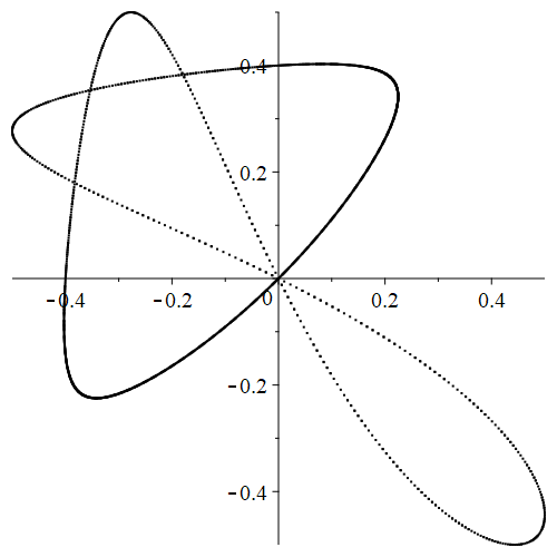
(a) Plot of $(\sin\psi_{a,n},\sin\psi_{b,n})$.

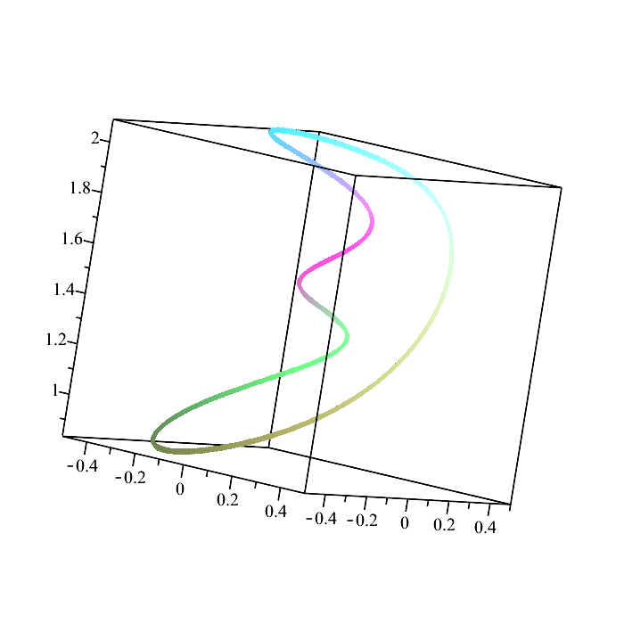
(b) 3D plot of $(\sin\psi_{a,n},\sin\psi_{b,n},u_{n})$.

Figure 5: 500 points on the orbit of the Brahmagupta angles for the main sequence.

As one more example of using elementary geometry to derive identities between elliptic functions, we start from a formula for the tangent of the bisected angle opposite side $a$, which is given on the first page of Schubert’s monograph [48], and in our notation reads

$$\tan\left(\frac{{\alpha}+{\beta}}{2}\right)=\frac{(s-b)(s-c)}{\Delta}.$$

Theorem 4.2.

The squares of the coordinates of the points on the orbit of the QRT map $\varphi$ associated wth the sequence (1.15) are given as rational functions of five adjacent quantities $f_{n}$ by

$$v_{n+2}^{2}=\frac{f_{n+1}^{2}f_{n+2}^{3}+f_{n+4}}{f_{n+3}(f_{n}^{2}-f_{n+2}f_{n+4})},\qquad v_{n+3}^{2}=\frac{f_{n+2}^{3}f_{n+3}^{2}-f_{n}}{f_{n+1}(f_{n+4}^{2}+f_{n}f_{n+2})}.$$ (4.5)

• In terms of the Schubert parameters, the tangent of the bisected angle for the $n$th triangle is $(P_{a,n}+M_{a,n})/(P_{a,n}M_{a,n}-1)$, while the right-hand side can be written in terms of ratios of $S_{n}$ and $T_{n}$ terms, and ultimately as $f_{n}f_{n+1}f_{n+2}/f_{n+4}$, so that this becomes an identity for signed quantities. Then substituting for the Schubert parameters from (3.5) and writing everything in terms of $f_{n}$ and $v_{n}$, this produces the formula

  $$\frac{1}{f_{n+4}}=\frac{f_{n+2}f_{n+3}\,v_{n+2}^{2}+1}{f_{n}^{2}f_{n+3}\,v_{n+2}^{2}-f_{n+1}^{2}f_{n+2}^{3}};$$

  the right-hand side above is a Möbius transformation of $v_{n+2}^{2}$, which is inverted to obtain the first expression in (4.5). An analogous calculation starting from the corresponding formula for the tangent of the bisected angle opposite side $b$ produces the second expression for $v_{n+3}^{2}$. ∎

Remark 4.3.

In principle one can use repeated application of the recurrence (2.44) in (4.5) to eliminate $f_{n+4},f_{n+3},f_{n+2}$ and write $v_{n+2},v_{n+3}$ as rational functions of $f_{n},f_{n+1}$ only, then use (2.45) to simplify the resulting formulae; this would be a rather tedious way to verify the 2-isogeny given by (2.52) in terms of these pairs of coordinates. Since it involves the product $(v_{n+2}v_{n+3})^{2}$, substituting for the latter with (4.5) and applying the same method provides an alternative proof of the identity (3.9), which is equivalent to the linear relation (3.8) for the signed lengths, although from the point of view of the logical progression of the paper this is a somewhat circular argument, since Lemma 3.1 was one of the key steps in showing that the quantities $f_{n}$ describe the geometry of the main sequence of Heron triangles as claimed.

5 Conclusions

Table 8: Prime factors of the Schubert parameters in the sporadic cases.

$n$	$M_{a}$	$P_{a}$	$X_{a}$	$M_{b}$	$P_{b}$	$X_{b}$
	$\tfrac{2^{3}\cdot 7\cdot 13}{3\cdot 17}$	$17$	$\tfrac{2^{4}\cdot 3}{7\cdot 13}$	$\tfrac{3\cdot 7\cdot 11}{2^{2}\cdot 5\cdot 13}$	$\tfrac{11\cdot 13\cdot 17}{2^{2}\cdot 3\cdot 5\cdot 7}$	$\tfrac{17}{5\cdot 11}$
*	$\tfrac{3^{2}\cdot 5\cdot 31}{2^{2}\cdot 7\cdot 17}$	$\tfrac{2^{2}\cdot 5\cdot 31}{3^{2}\cdot 17}$	$\tfrac{3^{2}\cdot 7}{5\cdot 17}$	$\tfrac{3\cdot 7\cdot 17}{5\cdot 19}$	$\tfrac{3\cdot 5\cdot 17\cdot 19}{2^{3}\cdot 7\cdot 31}$	$\tfrac{3\cdot 19\cdot 31}{2^{4}\cdot 5\cdot 17}$
**	$\tfrac{2^{3}\cdot 19\cdot 47}{3^{2}\cdot 11\cdot 23}$	$\tfrac{3^{2}\cdot 11\cdot 17\cdot 47}{2^{3}\cdot 7\cdot 19\cdot 23}$	$\tfrac{2\cdot 7\cdot 11\cdot 47}{17\cdot 19\cdot 23}$	$\tfrac{2^{4}\cdot 3^{2}\cdot 7\cdot 17\cdot 23}{5\cdot 11\cdot 19\cdot 97}$	$\tfrac{2\cdot 7\cdot 11\cdot 17\cdot 19}{5\cdot 23\cdot 97}$	$\tfrac{5\cdot 11\cdot 19\cdot 23}{2^{5}\cdot 3^{2}\cdot 97}$
***	$\tfrac{2^{2}\cdot 3\cdot 17\cdot 43\cdot 59}{5\cdot 11\cdot 13\cdot 19\cdot 23}$	$\tfrac{2^{3}\cdot 3\cdot 5\cdot 13\cdot 23\cdot 43}{11\cdot 19\cdot 41\cdot 59}$	$\tfrac{19\cdot 23\cdot 41\cdot 43}{5\cdot 11\cdot 13\cdot 17\cdot 59}$	$\tfrac{19\cdot 23\cdot 41\cdot 43}{2^{4}\cdot 3\cdot 7\cdot 11\cdot 59}$	$\tfrac{11\cdot 19\cdot 41\cdot 59}{7\cdot 17\cdot 23\cdot 43}$	$\tfrac{7\cdot 19\cdot 43\cdot 59}{2^{5}\cdot 3\cdot 11\cdot 17\cdot 23}$

Table 9: Prime factors of the semiperimeter, reduced side lengths and area in the sporadic cases.

$n$	$s$	$s-a$	$s-b$	$s-c$	$\Delta$
*	$3\cdot 7\cdot 13\cdot 17$	$2^{3}\cdot 5^{2}\cdot 17$	$3\cdot 7\cdot 13$	$2^{3}\cdot 11^{2}$	$2^{3}\cdot 3\cdot 5\cdot 7\cdot 11\cdot 13\cdot 17$
*	$2^{3}\cdot 7\cdot 19^{2}$	$2^{3}\cdot 3^{6}$	$5^{2}\cdot 7\cdot 31$	$17^{2}\cdot 31$	$2^{3}\cdot 3^{3}\cdot 5\cdot 7\cdot 17\cdot 19\cdot 31$
**	$2^{3}\cdot 3^{2}\cdot 11^{2}\cdot 19^{2}$	$2^{5}\cdot 3^{2}\cdot 5^{2}\cdot 7\cdot 17$	$23^{2}\cdot 47^{2}$	$7\cdot 17\cdot 97^{2}$	$2^{4}\cdot 3^{2}\cdot 5\cdot 7\cdot 11\cdot 17\cdot 19\cdot 23\cdot 47\cdot 97$
***	$17\cdot 23^{2}\cdot 59^{2}$	$5^{2}\cdot 7^{2}\cdot 13^{2}\cdot 41$	$2^{4}\cdot 3\cdot 11^{2}\cdot 43^{2}$	$2^{4}\cdot 3\cdot 17\cdot 19^{2}\cdot 41$	$2^{4}\cdot 3\cdot 5\cdot 7\cdot 11\cdot 13\cdot 17\cdot 19\cdot 23\cdot 41\cdot 43\cdot 59$

We have proved all the empirical observations on the infinite sequence of Heron triangles with two rational medians found by Buchholz and Rathbun in [7], and this led us to explicit formulae for the side lengths, rational medians and the area in terms of the Somos-5 sequences (1.14) and (1.15). The crux of our proof was to view the underlying elliptic curve as a complex torus, and construct an analytic embedding of this torus in the Schubert surface, such that the required algebraic identities for the two sets of Schubert parameters are valid for all complex values of the argument, and in particular at an infinite discrete set of points corresponding to the indices $n\in{\mathbb{Z}}$. The indices $n\geq 1$ provide infinitely many distinct triangles, while under the involution $n\to-n-4$ the indices $n\leq 0$ correspond to the same set of triangles repeated with reversed orientation via the symmetry $a\leftrightarrow b$, together with a finite number of singular values.

It would also be possible to prove Theorem 3.3 by purely algebraic means, using (2.44) and the 2-isogeny (2.52), but this would require extensive amounts of computer algebra, without providing much insight into the problem. Our hope was that the analytical approach would give a better understanding of the structure of the triangles in the main sequence, and suggest whether this might allow the sporadic solutions to be extended to other infinite families, perhaps by writing them in terms of different Somos sequences, as well as possibly shedding some light on the harder problem of showing why no perfect triangle exists. However, the detailed features of the solutions in the main sequence appear to rely on specific arithmetical properties of the group of rational points on the curve ${\cal C}$, and even the particular numerical values of the coordinates of the two generators, and we have been unable to generalize this to produce one or more other infinite families. Nevertheless, the prime factors of the Schubert parameters and reduced lengths for the sporadic triangles (see Tables 8 and 9) give tantalizing hints that there might be other families that these solutions could belong to, only with a different structure compared with the main sequence. A more extensive computer search, and the discovery of more new solutions, would provide further evidence in this direction, or otherwise suggest that these four solutions are truly sporadic.

Acknowledgments: This research was supported by Fellowship EP/M004333/1 from the Engineering & Physical Sciences Research Council, UK, and grant IEC\R3\193024 from the Royal Society. It is a pleasure to thank Chris Athorne and Claire Gilson for the opportunity to present a preliminary version of this work at the joint British Mathematical/Applied Mathematics Colloquium in Glasgow, and to thank Harry Braden for some helpful comments during the ICMS Integrable Systems Virtual Seminar in April 2021. All data generated or analysed during this study are included in this published article.

References

- [1] Y. Abdelaziz and J.-M. Maillard, Modular forms, Schwarzian conditions, and symmetries of differential equations in physics, J. Phys. A: Math. Theor. 50 (2017) 215203.
- [2] N.I Akhiezer, Elements of the Theory of Elliptic Functions, Translations of Mathematical Monographs, vol. 79, American Mathematical Society, 1990.
- [3] Z.F. Bácskái, R.H. Buchholz, R.L. Rathbun and M.J. Smith, Symmetries of triangles with two rational medians, (2003) http://citeseerx.ist.psu.edu/viewdoc/summary?doi=10.1.1.65.6533
- [4] M. Bershtein, P. Gavrylenko and A. Marshakov, Cluster Toda Chains and Nekrasov Functions, Theor. Math. Phys. 198 (2019) 157–188.
- [5] M. Bruschi, O. Ragnisco, P.M. Santini and T. Gui-Zhang, Integrable symplectic maps, Physica D 49 (1991) 273–294.
- [6] R.H. Buchholz, On Triangles with rational altitudes, angle bisectors or medians, PhD thesis, University of Newcastle, 1989.
- [7] R.H. Buchholz and R.L. Rathbun, An infinite set of Heron triangles with two rational medians, Amer. Math. Monthly 104 (1997) 107–115.
- [8] R.H. Buchholz and R.L. Rathbun, Heron triangles and elliptic curves, Bull. Austral. Math. Soc. 58 (1998) 411–421.
- [9] R.H. Buchholz and R.P. Stingley, Heron triangles with three rational medians, Rocky Mountain J. Math. 49 (2019) 405–417.
- [10] L.E. Dickson, History of the Theory of Numbers, Vol. II: Diophantine Analysis, Carnegie Institution, Washington, 1920.
- [11] C.L. Dodgson, Condensation of determinants, being a new and brief method for computing their arithmetical values, Proc. R. Soc. London 15 (1866) 150–155.
- [12] J.J. Duistermaat, Discrete Integrable Systems: QRT Maps and Elliptic Surfaces, Springer Monographs in Mathematics, vol. 304. Springer, 2010.
- [13] A. Dujella and J.C. Peral, Elliptic curves coming from Heron triangles, Rocky Mt. J. Math. 44 (2014) 1145–1160.
- [14] R. Eager, S. Franco and K. Schaeffer, Dimer models and integrable systems, J. High Energy Phys. 2012 (2012) 106.
- [15] N.D. Elkies, response to sci.math.research newsgroup posting, April 1995; now hosted on Google Groups at https://groups.google.com/g/sci.math.research/c/LHS1P8fn9Ek/m/uU6NC78fAJ
- [16] G. Everest, A. van der Poorten, I. Shparlinski and T. Ward, Recurrence Sequences, AMS Mathematical Surveys and Monographs, vol. 104, Amer. Math. Soc., Providence, RI, 2003.
- [17] Y.N. Fedorov and A.N.W. Hone, Sigma-function solution to the general Somos-6 recurrence via hyperelliptic Prym varieties, J. Integrable Systems 1 (2016) xyw012.
- [18] S. Fomin and A. Zelevinsky, Cluster algebras I: Foundations, J. Amer. Math. Soc. 15 (2002) 497–529.
- [19] S. Fomin and A. Zelevinsky, The Laurent Phenomenon, Adv. Appl. Math. 28 (2002) 119–144.
- [20] A.P. Fordy and R.J. Marsh, Cluster mutation-periodic quivers and associated Laurent sequences, J. Algebraic Combin. 34 (2011) 19–66.
- [21] A.P. Fordy and A.N.W. Hone, Discrete integrable systems and Poisson algebras from cluster maps, Commun. Math. Phys. 325 (2014) 527–584.
- [22] D. Gale, The strange and surprising saga of the Somos sequences, Mathematical Intelligencer 13 (1) (1991) 40–42; reprinted in Tracking the Automatic Ant, Springer, 1998.
- [23] E.H. Goins and D. Maddox, Heron triangles via elliptic curves, Rocky Mt. J. Math. 36 (2006) 1511–1526.
- [24] A.B. Goncharov and R. Kenyon, Dimers and cluster integrable systems, Ann. Sci. Éc. Norm. Supér. 46 (2013) 747–813.
- [25] M. Gross, P. Hacking, S. Keel and M. Kontsevich, Canonical bases for cluster algebras, J. Amer. Math. Soc. 31 (2018) 497–608.
- [26] R.K. Guy, Unsolved Problems in Number Theory, Springer-Verlag, New York, 1981.
- [27] A.N.W. Hone, Sigma function solution of the initial value problem for Somos 5 sequences, Trans. Amer. Math. Soc. 359 (2007) 5019–5034.
- [28] A.N.W. Hone, T.E. Kouloukas and C. Ward, On Reductions of the Hirota-Miwa Equation, SIGMA 13 (2017) 057.
- [29] A.N.W. Hone and C.S. Swart, Integrality and the Laurent phenomenon for Somos 4 and Somos 5 sequences, Math. Proc. Camb. Phil. Soc. 145 (2008) 65–85.
- [30] E.J. Ionascu, F. Luca and P. Stanica, Heron triangles with two fixed sides, J. Number Theory 126 (2007) 52–67.
- [31] S. Ismail, Perfect triangles on the curve , J. Austral. Math. Soc. 109 (2020) 68–80.
- [32] S. Ismail and Z. Eshkuvatov, Perfect Triangles: Rational Points on the Curve (The Unsolved Case), J. Phys. Conf. Ser. 1489 (2020) 012003.
- [33] D. Jogia, J.A.G. Roberts and F. Vivaldi, An algebraic geometric approach to integrable maps of the plane, J. Phys. A: Math. Gen. 39 (2006) 1133.
- [34] M. Kanki, J. Mada, K.M. Tamizhmani, T. Tokihiro, Discrete Painlevé II equation over finite fields, J. Phys. A: Math. Theor. 45 (2012) 342001.
- [35] M. Kanki, J. Mada, T. Mase and T. Tokihiro, Irreducibility and co-primeness as an integrability criterion for discrete equations, J. Phys. A: Math. Theor. 47 (2014) 465204.
- [36] P.H. van der Kamp, Somos-4 and Somos-5 are arithmetic divisibility sequences, J. Difference Equ. Appl. 22 (2016) 570–580.
- [37] T. Lam and P. Pylyavskyy, Laurent phenomenon algebras, Cam. J. Math. 4 (2012) 121–162.
- [38] K. Lee and R. Schiffler, Positivity for cluster algebras, Ann. Math. 182 (2015) 73–125.
- [39] The LMFDB Collaboration, The L-functions and modular forms database (2021) https://www.lmfdb.org/EllipticCurve/Q/102a1/
- [40] R. van Luijk, An elliptic K3 surface associated with Heron triangles, J. Number Theory 123 (2007) 92–119.
- [41] X. Ma, Magic determinants of Somos sequences and theta functions, Discrete Mathematics 310 (2010) 1–5.
- [42] S. Maeda, Completely integrable symplectic mapping, Proc. Japan Acad. Ser. A Math. Sci. 63 (1987) 198–200.
- [43] OEIS Foundation Inc. (2021), The On-Line Encyclopedia of Integer Sequences, http://oeis.org/A006721
- [44] A.J. van der Poorten and C.S. Swart, Recurrence Relations for Elliptic Sequences: every Somos 4 is a Somos , Bull. Lond. Math. Soc. (2005)
- [45] G.R.W. Quispel, J.A.G. Roberts and C.J. Thompson, Integrable mappings and soliton equations, Phys. Lett. A 126 (1988) 419–421.
- [46] G.R.W. Quispel, J.A.G. Roberts and C.J. Thompson, Integrable mappings and soliton equations II, Physica D 34 (1989) 183–192.
- [47] R. Robinson, Periodicity of Somos sequences, Proc. Amer. Math. Soc. 116 (1992) 613–619.
- [48] H. Schubert, Die Ganzzahligkeit in der algebraischen Geometrie, Spamersche Buchdruckerei, Leipzig, 1905.
- [49] J.H. Silverman, The Arithmetic of Dynamical Systems, Springer, 2007.
- [50] M. Somos, Problem 1470, Crux Mathematicorum 15 (1989) 208.
- [51] C.S. Swart, Elliptic curves and related sequences, PhD thesis, University of London, 2003.
- [52] T. Tsuda, Integrable mappings via rational elliptic surfaces, J. Phys. A: Math. Gen. 37 (2004) 2721.
- [53] Y. Uchida, Valuations of Somos 4 sequences and canonical local heights on elliptic curves, Math. Proc. Camb. Phil. Soc. 150 (2011) 385–397.
- [54] A.P. Veselov, Integrable Maps. Russ. Math. Surv. 46 (1991) 1–51.
- [55] M. Ward, Memoir on elliptic divisibility sequences, Amer. J. Math. 70 (1948) 31–74.
- [56] E.T. Whittaker and G.N. Watson, A Course of Modern Analysis, Cambridge University Press, 4th edition, 1927.