Thermal noise competes with turbulent fluctuations below millimeter scales

Abstract

Turbulent flows frequently accompany physical, chemical and biological processes, such as mixing, two-phase flow, combustion and even foraging by bacteria and plankton larvae, all of which are in principle subject to thermal fluctuations already on scales of several microns. Nevertheless the large separation between the millimeter scale at which turbulent fluctuations begin to be strongly damped and the mean free path of the fluid has been generally assumed to imply that thermal fluctuations are irrelevant to the turbulent dissipation range. Here we use statistical mechanical estimates to show that thermal fluctuations are not negligible compared to turbulent eddies in the dissipation range. Simulation of the Sabra shell model shows that intermittent bursts of turbulence lead to a fluctuating length scale below which thermal fluctuations are important: over three decades of length, from sub-millimeter scales down to the mean free path, thermal fluctuations coexist with hydrodynamics. Our results imply that thermal fluctuations cannot be neglected when modeling turbulent phenomena in the far dissipation range.

Thermal effects are known to play a prominent role in many physical, chemical and biological processes in molecular fluids. These include high Schmidt/Prandtl-number scalar mixing Donev et al. (2014a), droplet and bubble formation Chaudhri et al. (2014); Gallo et al. (2020), locomotion of micro-organisms Götze and Gompper (2010), combustion Lemarchand and Nowakowski (2004); Bhattacharjee et al. (2015), and others. Often the relevant flows are turbulent, in which case all current approaches to model these processes — high Schmidt-number scalar mixing Clay et al. (2018); Buaria et al. (2020), droplet and bubble formation Elghobashi (2019); Milan et al. (2020), cellular motility Durham et al. (2013); Wheeler et al. (2019), and combustion Donzis et al. (2010); Sreenivasan (2004); Driscoll (2008); Echekki and Mastorakos (2010) — focus on turbulent fluctuations due to fluid inertia damped by viscosity and ignore thermal effects completely. This neglect is commonly justified by the idea that there is a strong separation between hydrodynamic scales dominated by turbulent fluctuations and extremely small scales of order the mean-free path length where thermal fluctuations begin to play a role Von Neumann (1963). The smallest turbulent fluid scales below which eddies are damped by viscosity, known as the dissipation range, typically occurs at millimeter scales and there is currently intensive effort, by computation Khurshid et al. (2018); Gorbunova et al. (2020); Buaria and Sreenivasan (2020), theory Pauls and Ray (2020); Canet et al. (2017); Gibbon and Dubrulle (2021) and experiment Debue et al. (2018); Gorbunova et al. (2020); Debue et al. (2021), to understand the dynamics and statistics at these scales. The motivation ranges from unraveling the nature of turbulence itself, and the associated unsolved issue of formation of singularities Fefferman (2006), to the phenomena and practical applications mentioned above and others.

The basic underlying assumption in turbulent flows of a viscous dissipation range well-separated from thermal fluctuations is at first sight surprising. This seemingly contradicts the fluctuation-dissipation theorem of statistical physics (e.g. see de Zarate and Sengers (2006)), which implies that thermal fluctuations and dissipation should be intrinsically tied together, even in a far from equilibrium system where local thermal equilibrium can be justified. The neglect of thermal effects in the dissipation range is convenient; it allows one to use the Navier-Stokes partial differential equations exclusively to model the phenomena of interest and even this requires a computational tour de force for turbulent flows Khurshid et al. (2018); Gorbunova et al. (2020); Buaria and Sreenivasan (2020). On the other hand, the hydrodynamic equations consistent with the fluctuation-dissipation theorem for fluids locally in thermal equilibrium were formulated already by Landau and Lifshitz in 1959 Landau and Lifshitz (1959); de Zarate and Sengers (2006), and the effects of thermal fluctuations measured at the onset of Rayleigh-Bénard convection Wu et al. (1995). As far as turbulence is concerned, most prior discussions Hosokawa (1976); Ruelle (1979); Macháček (1988) suggest that thermal noise plays only only a secondary role in the selection and uniqueness of the stationary measures characterizing turbulence. To what extent are these seemingly abstract considerations relevant to real flows, especially given the large separation in scales between the mean free path and those where hydrodynamic dissipation occurs?

The purpose of this Letter is to provide theoretical arguments and numerical evidence that thermal noise effects manifest throughout the turbulent dissipation range, in contradiction to widespread belief. Our results imply that a nontrivial interplay between turbulent and thermal fluctuations must occur at small scales for nearly all flows in Nature and in the laboratory. Our results support pioneering ideas of Betchov Betchov (1957, 1961, 1964), who reached similar conclusions already in 1957, and extend them to account for the effects of inertial-range intermittency.

In the low Mach number ($Ma$) limit, fluctuating hydrodynamics adds a stochastic stress term ${\mbox{\boldmath$\nabla$}}\cdot{\mbox{\boldmath$\tau$}}$ to the incompressible Navier-Stokes equation for the velocity ${\bf u}$ satisfying Forster et al. (1976, 1977); Usabiaga et al. (2012); Donev et al. (2014b) ${\mbox{\boldmath$\nabla$}}{\mbox{\boldmath$\cdot$}}{\bf u}=0$ and

$$\partial_{t}{\bf u}+({\bf u}\cdot{\mbox{\boldmath$\nabla$}}){\bf u}=-{\mbox{\boldmath$\nabla$}}p+\nu\Delta{\bf u}+{\mbox{\boldmath$\nabla$}}\cdot{\mbox{\boldmath$\tau$}}.$$ (1)

In accord with the general fluctuation-dissipation relation, the stress $\tau_{ij}({\bf x},t)$ which models thermal fluctuations is a Gaussian random field with mean zero and covariance

$$\langle\tau_{ij}({\bf x},t)\tau_{kl}({\bf x}^{\prime},t^{\prime})\rangle = \frac{2\nu k_{B}T}{\rho}\left(\delta_{ik}\delta_{jl}+\delta_{il}\delta_{jk}-\frac{2}{3}\delta_{ij}\delta_{kl}\right)$$ (3)

$$\hskip 30.0pt\times\delta^{3}({\bf x}-{\bf x}^{\prime})\delta(t-t^{\prime}),$$

which is proportional to the kinematic viscosity $\nu,$ the dissipative transport coefficient of the fluid, and absolute temperature $k_{B}T$ in energy units set by Boltzmann’s constant $k_{B}$. The other parameter appearing in (3) is $\rho,$ the mass density of the fluid. It is precisely Eq.(1) that one must solve numerically Usabiaga et al. (2012); Donev et al. (2014b), or otherwise, in order to model molecular fluids at low Mach number.

Noise estimate. We now rehearse standard arguments Von Neumann (1963) that thermal effects in fluids become important only at scales comparable to the mean free path length $\lambda_{mfp}$, and then explain why these arguments are not valid. The velocity fluctuations at length scale $\ell$ from thermal fluctuations can be estimated as

$$u_{\ell}^{th}\sim c_{th}/(n\ell^{3})^{1/2}=c_{th}(\ell_{int}/\ell)^{3/2},$$ (4)

where $c_{th}$ is the speed of sound, $n$ is the number density and $\ell_{int}$ is the typical interparticle distance. The standard argument asks when thermal fluctuations at the scale $\ell$ are of the same order as a typical flow velocity $u$; equating them, we find that $\ell\sim\ell_{int}(Ma)^{-2/3}$, where $Ma=u/c_{th}$ is the corresponding Mach number. By this argument, thermal fluctuations become important only at scales comparable to $\ell_{int}$, which is of the same order as $\lambda_{mfp}$ in liquids and $\ll\lambda_{mfp}$ in gases. Even for $Ma\ll 1,$ the thermal fluctuation velocities are still much smaller than $u$ until $\ell$ becomes comparable to $\ell_{int}$, and so can be neglected. The flaw in this argument is that the thermal velocity at scale $\ell$ should not be compared with the mean velocity or r.m.s. velocity $u$ of the eddies of largest size $L$. Instead it is more appropriate to compare $u^{th}_{\ell}$ with the r.m.s velocity $u_{\ell}$ of turbulent eddies at the same scale $\ell$. In the dissipation range $u_{\ell}$ drops exponentially with decreasing $\ell$ so that thermal fluctuations very quickly become competitive with turbulent fluctuations, as is shown by the following quantitative estimate.

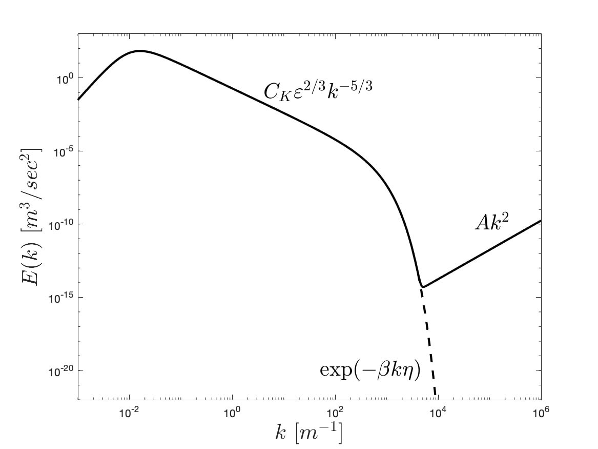
Figure 1: Plot of the model turbulent energy spectrum (5) for the parameters of the atmospheric boundary layer (7) and for a typical Reynolds number $Re=10^{7}$, as a solid line. The dashed line is the spectrum with no thermal noise.

We consider a standard model of the turbulent energy spectrum devised by von Kármán Von Kárḿan (1948), supplemented with an exponential factor to represent decay of turbulent fluctuations due to viscous effects. The estimate (4) of thermal velocity fluctuations can be equivalently restated as a $k^{2}$ equipartition energy spectrum, as first noted for equilibrium fluids in 3D by Lee Lee (1952), and Hopf Hopf (1952). The entire model spectrum then becomes

$$E(k)=C_{K}(\varepsilon L)^{2/3}\frac{L^{5}k^{4}}{(1+(kL)^{2})^{17/6}}\exp(-\beta k\eta)+Ak^{2},$$ (5)

where $C_{K}$ is the Kolmogorov constant, $\beta$ is the exponential decay rate in the far dissipation range and $A=\frac{4\pi}{(2\pi)^{3}}\frac{k_{B}T}{\rho}$ is the factor associated to thermal fluctuations in 3D. This model is plotted in Fig.1 with parameter values appropriate to the atmospheric boundary layer (ABL) Garratt (1994)

$$L=10^{5}\ cm,\quad\varepsilon=400\ cm^{2}/sec^{3},\quad\nu=0.15\ cm^{2}/sec,$$ (6)

$$\rho=1.2\times 10^{-3}\ g/cm^{3},\quad T=300^{\circ}K,$$ (7)

and with typical values of $\beta=7$ Khurshid et al. (2018) and $C_{K}=1.6$ Donzis and Sreenivasan (2010). One can see in Fig.1 the familiar regimes of turbulent flow, the inertial range with $E(k)\propto k^{-5/3}$, which transitions into the dissipation range with $E(k)\propto\exp(-\beta k\eta)$ around the Kolmogorov scale $\eta=(\nu^{3}/\epsilon)^{1/4}\sim 0.5\ \mathrm{mm}$. However, the model (5) predicts that once thermal fluctuations are included, this exponential decay is completely replaced by the $k^{2}$ equipartition spectrum. The presence of this thermal component on top of the turbulent spectrum does not automatically follow from the inclusion of thermal fluctuations in the dynamical equations (1), but can arise through the separation of time-scales, if it turns out that viscosity and thermal noise are more dominant than the nonlinear term in (1) for dissipation-range scales. Thus it is necessary to study this issue quantitatively, which we do below. We may note that thermal fluctuations have been considered already in numerical simulations of superfluid turbulence using Gross-Pitaevskii equation Shukla et al. (2019), and similar equipartition spectra observed.

We can estimate on order of magnitude the wavenumber $k_{eq}$ at which exponential decay is overtaken by thermal equipartition just by equating the two spectra, as $u_{\eta}^{2}\eta\mathrm{e}^{-k\eta}\sim\frac{k_{B}T}{\rho}k^{2}$ where $u_{\eta}=(\varepsilon\nu)^{1/4}$ is the Kolmogorov velocity. This leads to a formula for $k_{eq}$ of the form

$$(k_{eq}\eta)^{2}\mathrm{e}^{k_{eq}\eta}=1/\theta_{K}$$ (8)

in which appears the dimensionless ratio

$$\theta_{K}=\frac{k_{B}T}{\rho u_{\eta}^{2}\eta^{3}}.$$ (9)

The quantity $\theta_{K}$ is a new dimensionless number group that characterizes the turbulent flow, in addition to the Reynolds number $Re.$ Substituting into (8) the values of parameters (7) characteristic of the ABL, we arrive at the value $\theta_{K}=2.83\times 10^{-8}.$ It is then easy to calculate from (8) that $k_{eq}\eta\doteq 11,$ which in the ABL corresponds to a length $\ell_{eq}\simeq 49\ \mu$m. In fact, due to the rapid increase of the exponential in (8), this equipartition scale $\ell_{eq}$ is very insensitive to the precise value of $\theta_{K}$ and always takes a value only a factor of 10 or so smaller than $\eta.$ This result is strikingly different from the naive expectation that thermal effects become important only at length scales comparable to the mean free path, which is $\lambda_{mfp}=68\ \mathrm{nm}\sim\eta/10^{4}$ in the ABL. Alternatively, using parameters from water experiments of Debue et al. (2018), $\eta=16\ \mu\mathrm{m}$ and $\theta_{K}\doteq 2.5\times 10^{-7},$ we estimate that thermal fluctuations should be significant from just below $16\ \mu\mathrm{m}$ down to $\lambda_{mfp}\doteq 0.25\ \mathrm{nm}$. In summary, naturally occurring and practically relevant turbulent flows possess several decades of length scales where a hydrodynamic approximation is justified and yet fluctuations are dominated by thermal effects.

The previous arguments and conclusions are nearly identical to those presented by Betchov Betchov (1957), except that, rather than an energy spectrum exhibiting exponential decay, he assumed a fast power-law decay $\sim k^{-n}$ with $n\doteq 6$-$7$ in the far-dissipation range, as predicted by contemporary theories of Heisenberg Heisenberg (1948) and others. To assess these arguments and to extend them beyond the energy spectrum to higher-order moments sensitive to intermittency effects, we now consider a simple dynamical model of turbulence which is believed to capture the nontrivial multifractal scaling properties of turbulence.

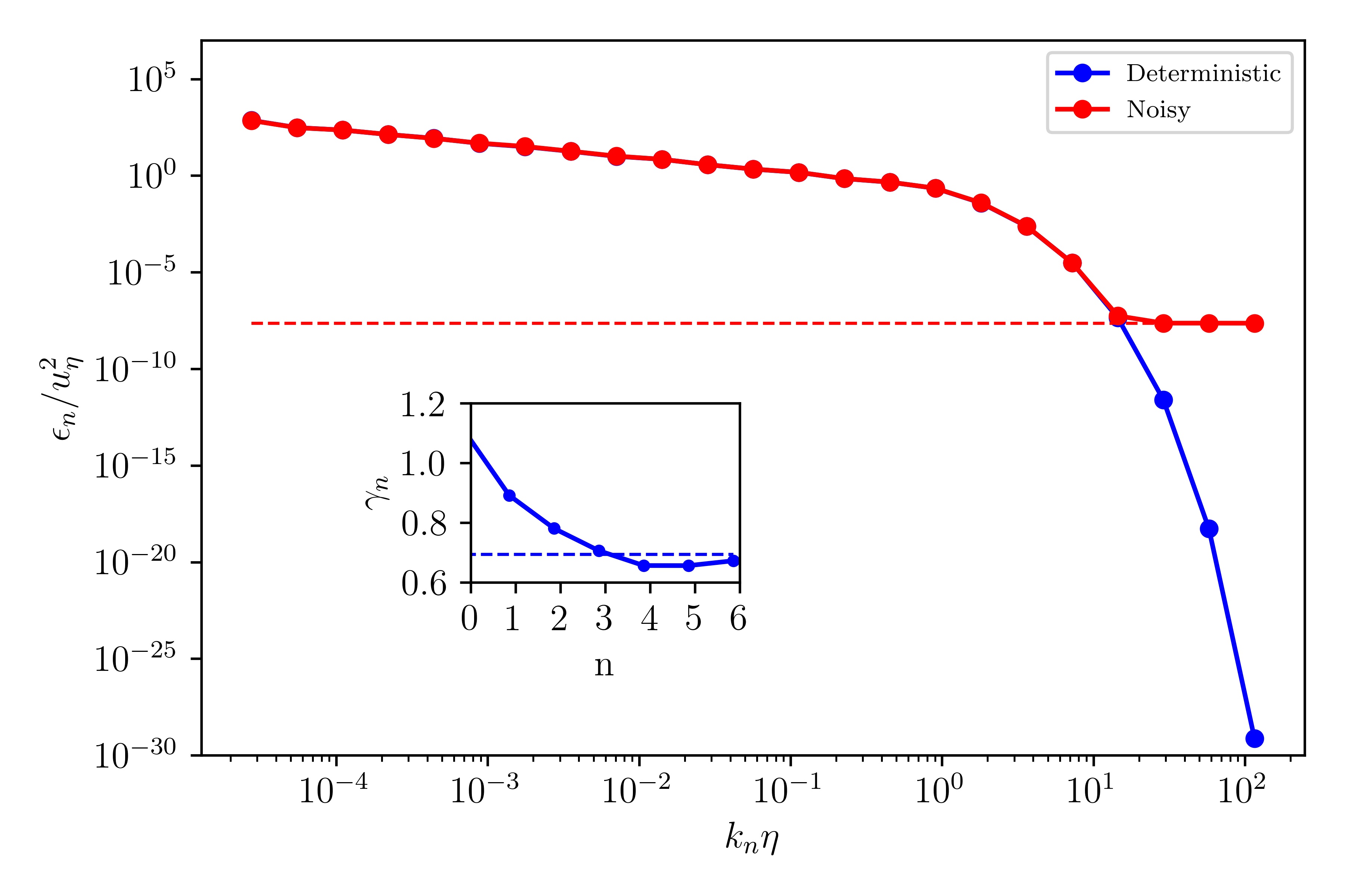
Figure 2: The energy spectrum of the deterministic model (-----), noisy model (-----), and the thermal equipartition value $2\theta_{K}$ (- - -). Inset: The local stretching exponents (11) for the deterministic model spectrum ($\bullet$) and its theoretical value in (10) (- - -).

Numerical simulations. To further understand the interplay of turbulent and thermal fluctuations we turn to numerical simulations. Unfortunately, direct numerical simulations of the fluctuating Navier-Stokes equation (1) with sufficient range of scales to study how rare intense events at high Reynolds number interact with thermal fluctuations are not yet feasible, even with the largest supercomputers in the world. We therefore resort to shell models, simplified dynamical systems that are widely used as surrogates of Navier-Stokes equations in order to perform high Reynolds number simulations Biferale (2003) of scaling properties. In particular, we employ the Sabra shell model L’vov et al. (1998) supplemented with stochastic terms controlled by ”temperature“ to represent thermal noise. It is defined by a set of coupled nonlinear stochastic ODEs that describe evolution of complex variables $u_{n}$ defined at discrete wavenumbers $k_{n}=k_{0}2^{n},$ $n=0,1,2,...,N$. Here $u_{n}$ represents the “velocity” of an eddy of size $1/k_{n}$. At large times the Sabra model with fixed forcing attains a statistical steady-state with constant flux of energy $E=\sum_{n}\epsilon_{n}=\frac{1}{2}\sum_{n}|u_{n}|^{2}$ due to the cascade across scales in the inertial range. To understand the relative importance of turbulent and thermal fluctuations, we simulated the system for times large enough to represent the steady-state with the parameters in (7) for the ABL, achieving the Reynolds number $Re\sim 10^{6}$. The simulation was done twice, once with thermal noise, once without. Further details on stochastic Sabra model and our numerical stochastic integration scheme, as well as convergence tests can be found in Supplementary information and elsewhere Eyink et al. (2021).

Discussion of results. The numerical results confirm our basic claim that thermal equipartition is achieved at scales close to $\eta/10$. This can be readily seen in Fig. 2, which depicts the mean energy spectrum $\bar{\epsilon}_{n}=1/2\langle|u_{n}|^{2}\rangle$ of the deterministic and noisy models. Note that shell models describe fluids effectively in $0$ space dimensions, so that equipartition corresponds to a constant value $(1/2)\varrho\langle|u_{n}|^{2}\rangle=k_{B}T,$ or $1/2\langle|u_{n}|^{2}\rangle=\theta_{K}$ in dimensionless Kolmogorov units. The deterministic model in the dissipation range displays stretched-exponential decay

$$\langle\epsilon_{n}\rangle\sim\exp(-c(k_{n}\ell_{K})^{\gamma}),\quad\gamma=\log_{2}\left(\frac{1+\sqrt{5}}{2}\right)$$ (10)

which was verified by plotting local stretching exponents

$$\gamma_{n}=\log_{2}\left|\ln\langle|u_{n+1}|^{2}\rangle\right|-\log_{2}\left|\ln\langle|u_{n}|^{2}\rangle\right|$$ (11)

(see Inset of Fig. 2). Such decay is expected for deterministic shell models Schörghofer et al. (1995); L’vov et al. (1998), but is not observed at all once thermal noise is included. The stretched exponential decay is then completely erased at shell-numbers above an equilibration scale $N_{e}=4$, where the modal energy is close to the equipartition value $\theta_{K}$. This equilibration wavenumber is just 16 times larger than the Kolmogorov wavenumber. It should be emphasized that our shell model must underestimate how rapidly the dissipation range is overtaken by thermal noise in comparison to true hydrodynamic turbulence. Indeed, the latter has a faster exponential spectral decay in the dissipation range Khurshid et al. (2018) compared to stretched-exponential for the shell model and, furthermore, the equipartition spectrum $E(k)$ is rising in hydrodynamic turbulence $\propto k^{2}$ and is decaying as $E(k_{n}):=\bar{\epsilon}_{n}/k_{n}\sim\theta_{K}/k_{n}$ in the shell model.

In contrast to the dissipation range spectrum for the noisy model, the inertial range energy spectrum shown in Fig. 2 is seemingly unchanged by thermal noise, which is an indication that the deterministic model is adequate for modeling fluctuations in the inertial range. The latter is known to exhibit intermittency realized through bursts that form at large scales and propagate to the dissipation range. Such bursts should be expected to cause the equilibration shell-number $N_{e}$ to fluctuate strongly in time. To investigate this issue, we defined an instantaneous equilibration shell-number $N_{e}(u)$ as the smallest integer such that time-averages of $\epsilon_{n}$ over one Kolmogorov time are below $2\theta_{K}$ for all $n\geq N_{e}(u)$. We illustrate this concept in Fig. 3, which plots the modal energy averaged over one Kolmogorov time as a function of wavenumber, for one typical shell-model realization and two extreme ones. We interpret the two extreme events as a large burst pushing $N_{e}(u)$ to a high value and as a deep lull allowing $N_{e}(u)$ to recede to a lower value. The underlying picture of intermittency is accepted for turbulence both in Navier-Stokes equation and in shell models, where it is attributed to self-similar solutions Daumont et al. (2000); Mailybaev (2013) that in the inviscid limit propagate in finite time to infinite wavenumbers. The same mechanism underlies the fluctuating nature of the “local viscous shellnumber” in the deterministic model

$$N_{vis}(u):=\min\left\{n:\,\frac{|u_{n}|}{\nu k_{n}}\leq 1\right\},$$ (12)

defined in analogy to the “local viscous/cutoff length” $\eta({\bf x},t)\sim\frac{\nu}{\delta_{\eta}u({\bf x},t)}$ of hydrodynamic turbulence Paladin and Vulpiani (1987); Schumacher (2007).

To characterize the statistical properties of the equilibration $N_{e}(u)$ and viscous $N_{vis}(u)$ scales we plot the probability density function (PDF) of their temporal fluctuations for the noisy Sabra model in Fig. 4. The PDF of $N_{e}(u)$ is well approximated at the core of the distribution by a discrete Gaussian $p(n)=e^{-(n-2)^{2}/2}/\Theta$ Agostini and Améndola (2019). This is somewhat surprising given the obvious asymmetry between small and large scales, but presumably such asymmetry is evidenced better in the extreme tails of the PDF which are not well-resolved with our data from 300 turnover times. Plotted as well in Fig. 4 is the PDF of $N_{vis}(u),$ defined as in (12). This PDF is plotted together with a standard multifractal model of the type developed for deterministic Navier-Stokes Biferale (2008), here constructed using the ansatz Bowman et al. (2006)

$$N_{vis}(h)={\rm Round}\left[\log_{2}(Re)\left(\frac{1}{1+h}-\frac{3}{4}\right)\right],$$ (13)

where “Round” denotes rounding to the nearest integer, and the PDF of the Hölder exponent $h$ is taken to be $P(h)\propto Re^{D(h)/(1+h)}$ for multifractal dimension spectrum $D(h)=\min_{p}\{ph-\zeta(p)\}$ with $\zeta(p)$ evaluated from our numerical simulation (see Fig. 5). The multifractal model is in reasonable agreement with the PDF of $N_{visc}$. Furthermore, for each realization that we used to calculate the PDF’s of $N_{visc}(u)$ and $N_{e}(u)$ we calculated a shift $\Delta N(u)=N_{visc}(u)-N_{e}(u)$ and its probability distribution in the steady-state. This distribution is peaked at $\Delta n=3$ and indeed supports an interpretation of the fluctuations of both $N_{visc}$ and $N_{e}$ being due to bursting nature of the inertial range. A reasonable interpretation is that, in each realization, the fluctuating viscous scale is followed by a stretched exponential decay, which gets overtaken within just a couple of shells by equipartition at the level of thermal energy $\theta_{K}$.

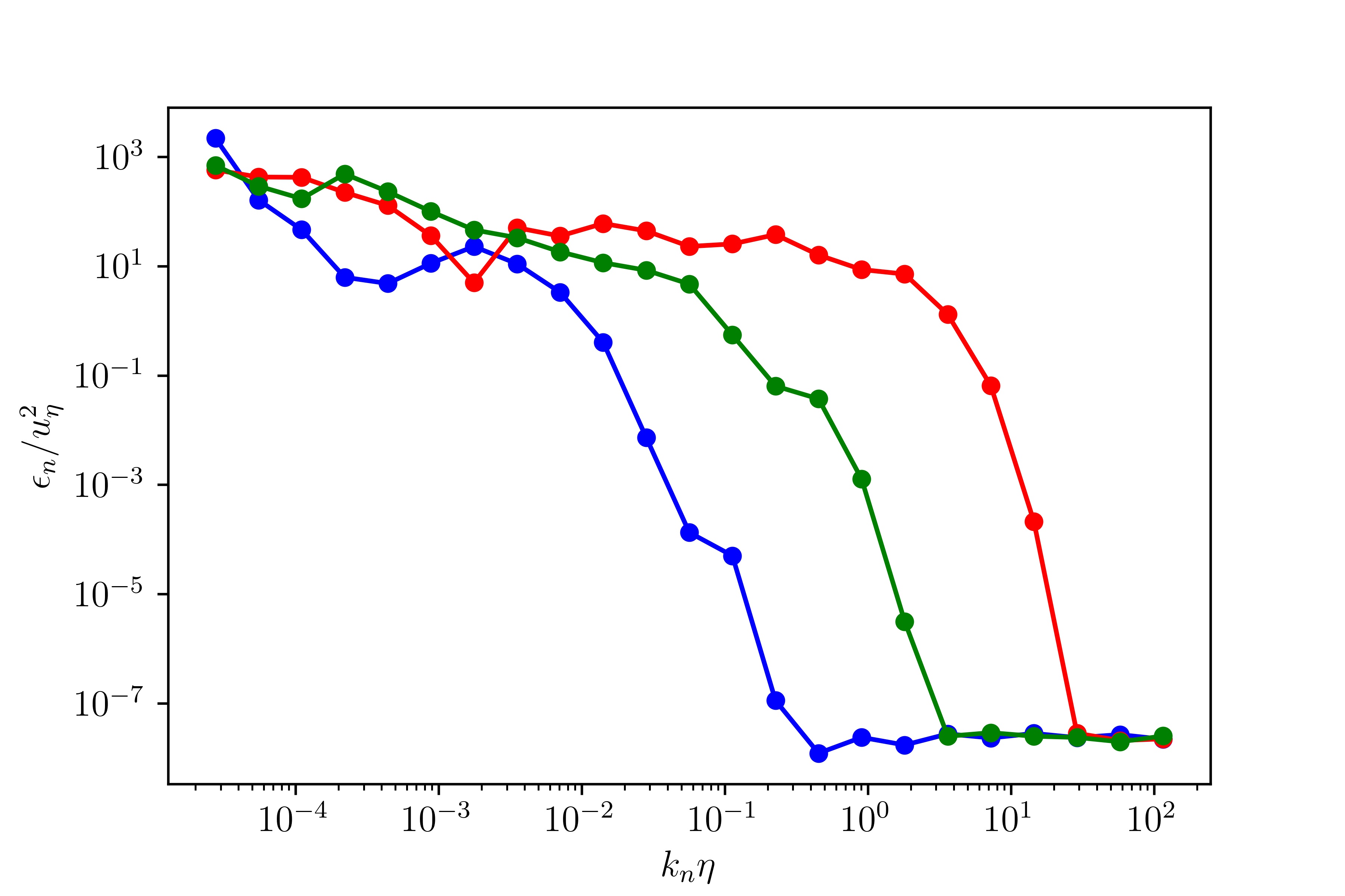
Figure 3: Modal energies of a lull (blue), a burst (red) and a typical realization (green), averaged over 1 Kolmogorov time, plotted versus $n$.

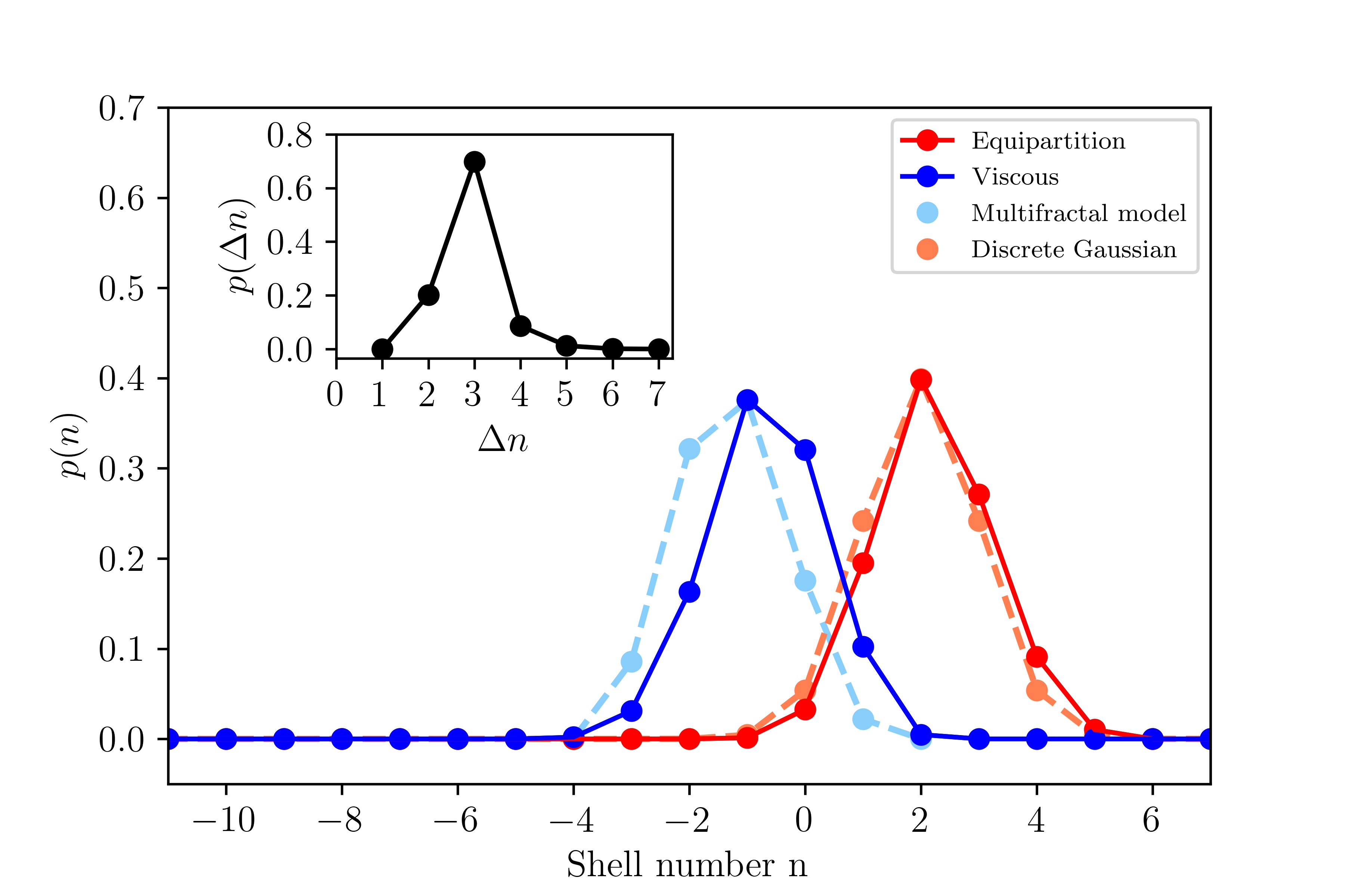
Figure 4: PDF’s of $N_{vis}(u)$ (blue) and $N_{e}(u)$ (red), along with a simple multifractal model for the PDF of $N_{vis}(u)$ (pale blue) and a fit by a discrete Gaussian distribution for the PDF of $N_{e}(u)$ (pale red). Inset: The PDF of the shift $\Delta N(u)$ in each realization. Standard errors of the mean for $N_{vis}(u)$ and $N_{e}(u)$ are smaller than the marker size.

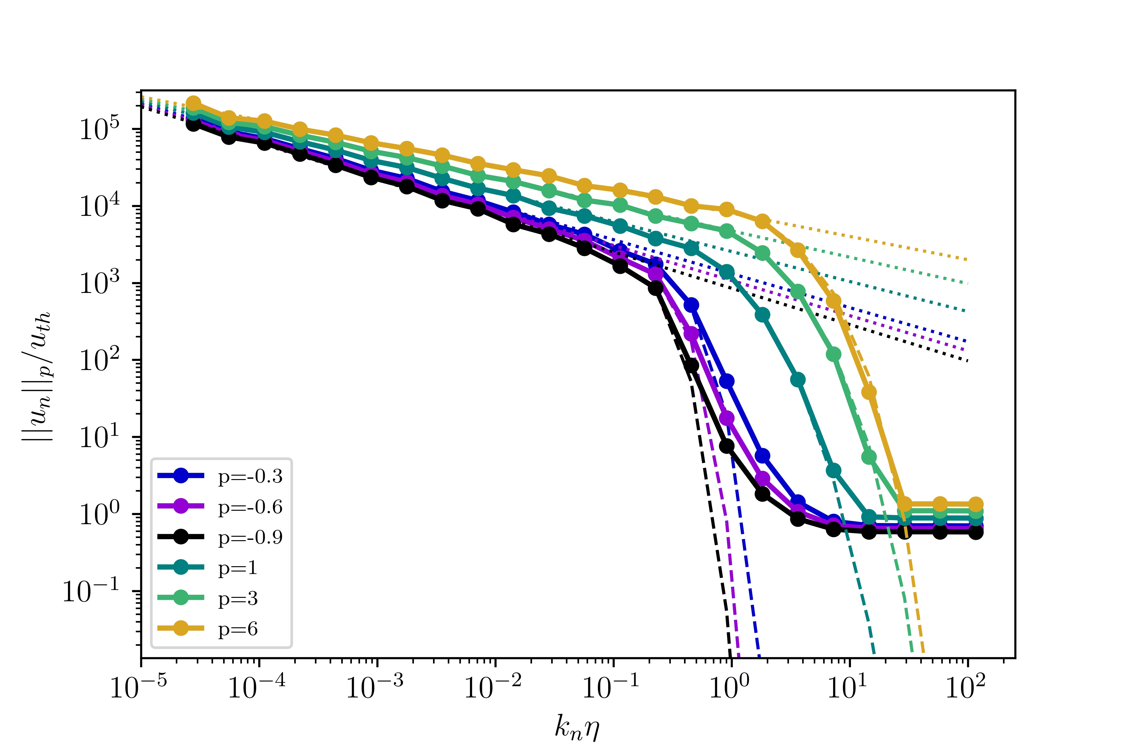
Figure 5: Structure functions for the deterministic model (dashed lines), for the noisy model (solid lines), and power-law fits in the inertial range (dotted lines).

The fluctuating nature of the equilibration scale $N_{e}(u)$ has important implications for the scale at which thermal effects appear in statistical averages. We consider the velocity structure functions, which we define as

$$\|u_{n}\|_{p}=\langle|u_{n}|^{p}\rangle^{1/p}$$ (14)

with a $p$-th root. Here $\langle\cdot\rangle$ denotes the steady-state average. Just as for the deterministic Sabra model L’vov et al. (1998), the noisy Sabra model exhibits power-law decay of structure functions with wavenumber, $\|u_{n}\|_{p}\propto k_{n}^{-\sigma(p)}$, where $\sigma(p)=\zeta(p)/p$ in terms of the standard exponents $\zeta(p)$, as shown in Fig. 5. To the accuracy of our calculation, the corresponding exponents $\sigma(p)$ for noisy and deterministic models are indistinguishable.

The inertial range intermittency is typically associated with nonlinear dependence of scaling exponents $\sigma(p)$ on $p$. Looking at structure functions with varying $p$ is also helpful for elucidation of the interplay of intermittency and noise. Higher positive values of $p$ assign a higher weight to events with larger value of $|u_{n}|$. In contrast negative values of $p$ shift weight to events with smaller values of $|u_{n}|$. This effect is clearly seen in Fig. 5, where one can read off the cut-off shellnumber $N_{e}(p)$ at which the $p$th structure-function attains its equipartition value $[\Gamma(1+\frac{p}{2})]^{1/p}\theta_{K}$. Evidently $N_{e}(p)$ exhibits strong $p$-dependence, with smaller $N_{e}(p)$ for negative values of $p$, and larger values of $N_{e}(p)$ for large positive $p$. Significantly, for negative values of $p$, thermal effects can be seen even at length scales above $\eta,$ inside the traditional inertial range. This suggests that a similar result should hold for the fluctuating Navier-Stokes equation, but experimental observation will be extremely challenging since the small magnitude of the thermal velocities, 3-4 orders of magnitude less than the Kolmogorov velocity $u_{\eta},$ will require very high precision of velocity measurements to be resolved.

Effect of spatial dimension. Up to now, we have ignored the potentially profound effect of space dimensionality $d$ on the character of fluctuating hydrodynamics. This effect can be simply understood by the estimate $u_{\ell}^{th}\sim(k_{B}T/\rho\ell^{d})^{1/2}$ for the magnitude of a thermal velocity fluctuation at length-scale $\ell$ in space-dimension $d$. It follows that the Reynolds number of the fluctuating hydrodynamic equation (1) in the thermal equipartition regime is

$$Re^{th}_{\ell}:=\frac{u_{\ell}^{th}\ell}{\nu}=\left(\frac{k_{B}T}{\rho\nu^{2}\ell^{d-2}}\right)^{1/2}$$

at length-scale $\ell$. Clearly for $d>2,$ $Re_{\ell}^{th}$ becomes increasing large with decreasing scale $\ell$. For $d<2$ $Re_{\ell}^{th}$ becomes smaller with decreasing $\ell$. This fact is well-known and can be obtained by more sophisticated renormalization group analysis Forster et al. (1976, 1977), according to which thermal fluids are UV asymptotically free for $d<2$ but UV strongly coupled for $d>2.$ These considerations apply to our shell model which has effectively $d=0$ and, indeed, we observe in our simulations that the noisy turbulent model becomes almost UV free at high-wavenumbers, with individual shell modes $u_{n}$ governed to good approximation by independent linear Langevin equations. Since 3D fluctuating hydrodynamics instead becomes strongly coupled in the UV, it might be doubted that our shell model properly represents the physics at scales where thermal fluctuations become important. However, the justification for our shell model lies in the extremely small values of $u_{\ell}^{th}$ for turbulent flows at scales $\ell\lesssim\eta.$ A dimensionless measure of this smallness is $Re^{th}_{\eta}=\theta_{K}^{1/2},$ which is of order $10^{-4}$ in the atmospheric boundary layer. A general calculation Eyink et al. (2021) confirms that fluctuating hydrodynamics for any molecular fluid in $d=3$ will remain weakly coupled until $\ell$ is comparable to the size of a molecule! Thus, the strong-coupling regime in the model at scales smaller than this is of no physical relevance.

Conclusion. In this Letter we provided theoretical order of magnitude estimates, corroborated by numerical simulations of the Sabra shell model of the turbulent cascade that thermal noise cannot be neglected in the dissipation range of incompressible turbulence, in contrast to the naive expectation that thermal effects are only relevant in molecular fluids at scales comparable to the mean free path length Von Neumann (1963). Our arguments and numerical results thus confirm and extend the prescient ideas of Betchov Betchov (1957, 1961, 1964). At the moment there are almost no experimental measurements below the Kolmogorov length to challenge the naive expectation that thermal noise becomes important only at the scale of the mean free path. However, there are many practically relevant processes that take place at sub-Kolmogorov scales of turbulent flow and therefore there is an urgent need for new experimental methods that can probe velocity fluctuations at those small scales with high accuracy to check the predictions made here. Perhaps the first evidence of thermal effects will be indirect, through the competing effects of turbulent and thermal fluctuations on the various physical phenomena strongly sensitive to sub-Kolmogorov turbulent scales. For example, we expect to see the influence of thermal noise on the Batchelor range of high Schmidt-number passive scalars, which extends well below the Kolmogorov scale. Another implication of our results is that there should be a possibly subtle influence of thermal noise on the inertial range of turbulence, through sensitivity of the equations of motion to perturbations Mailybaev (2016); Thalabard et al. (2020).

This work was supported by the Simons Foundation through Grant number 662985 (NG) and Grant number 663054 (GE).

References

- Donev et al. (2014a) A. Donev, T. G. Fai, and E. Vanden-Eijnden, Journal of Statistical Mechanics: Theory and Experiment 2014, P04004 (2014a).
- Chaudhri et al. (2014) A. Chaudhri, J. B. Bell, A. L. Garcia, and A. Donev, Physical Review E 90, 033014 (2014).
- Gallo et al. (2020) M. Gallo, F. Magaletti, D. Cocco, and C. M. Casciola, Journal of Fluid Mechanics 883 (2020).
- Götze and Gompper (2010) I. O. Götze and G. Gompper, Physical Review E 82, 041921 (2010).
- Lemarchand and Nowakowski (2004) A. Lemarchand and B. Nowakowski, Molecular Simulation 30, 773 (2004).
- Bhattacharjee et al. (2015) A. K. Bhattacharjee, K. Balakrishnan, A. L. Garcia, J. B. Bell, and A. Donev, The Journal of chemical physics 142, 224107 (2015).
- Clay et al. (2018) M. Clay, D. Buaria, P. Yeung, and T. Gotoh, Computer Physics Communications 228, 100 (2018).
- Buaria et al. (2020) D. Buaria, M. P. Clay, K. R. Sreenivasan, and P. Yeung, arXiv preprint arXiv:2004.06202 (2020).
- Elghobashi (2019) S. Elghobashi, Annual Review of Fluid Mechanics 51, 217 (2019).
- Milan et al. (2020) F. Milan, L. Biferale, M. Sbragaglia, and F. Toschi, Journal of Computational Science 45, 101178 (2020).
- Durham et al. (2013) W. M. Durham, E. Climent, M. Barry, F. De Lillo, G. Boffetta, M. Cencini, and R. Stocker, Nature communications 4, 1 (2013).
- Wheeler et al. (2019) J. D. Wheeler, E. Secchi, R. Rusconi, and R. Stocker, Annual review of cell and developmental biology 35, 213 (2019).
- Donzis et al. (2010) D. A. Donzis, K. Sreenivasan, and P. Yeung, Flow, turbulence and combustion 85, 549 (2010).
- Sreenivasan (2004) K. Sreenivasan, Flow, turbulence and combustion 72, 115 (2004).
- Driscoll (2008) J. F. Driscoll, Progress in Energy and Combustion Science 34, 91 (2008).
- Echekki and Mastorakos (2010) T. Echekki and E. Mastorakos, Turbulent Combustion Modeling: Advances, New Trends and Perspectives, Fluid Mechanics and Its Applications (Springer Netherlands, 2010).
- Von Neumann (1963) J. Von Neumann, in Collected Works of John Von Neumann, Vol.6: Theory of Games, Astrophysics, Hydrodynamics and Meteorology, edited by A. Taub (Pergamon Press, Oxford, 1963) pp. 437–472.
- Khurshid et al. (2018) S. Khurshid, D. A. Donzis, and K. R. Sreenivasan, Physical Review Fluids 3, 082601 (2018).
- Gorbunova et al. (2020) A. Gorbunova, G. Balarac, M. Bourgoin, L. Canet, N. Mordant, and V. Rossetto, Physical Review Fluids 5, 044604 (2020).
- Buaria and Sreenivasan (2020) D. Buaria and K. R. Sreenivasan, arXiv preprint arXiv:2004.06274 (2020).
- Pauls and Ray (2020) W. Pauls and S. S. Ray, Journal of Physics A: Mathematical and Theoretical 53, 115702 (2020).
- Canet et al. (2017) L. Canet, V. Rossetto, N. Wschebor, and G. Balarac, Physical Review E 95, 023107 (2017).
- Gibbon and Dubrulle (2021) J. Gibbon and B. Dubrulle, arXiv preprint arXiv:2102.00189 (2021).
- Debue et al. (2018) P. Debue, D. Kuzzay, E.-W. Saw, F. Daviaud, B. Dubrulle, L. Canet, V. Rossetto, and N. Wschebor, Physical Review Fluids 3, 024602 (2018).
- Debue et al. (2021) P. Debue, V. Valori, C. Cuvier, F. Daviaud, J.-M. Foucaut, J.-P. Laval, C. Wiertel, V. Padilla, and B. Dubrulle, Journal of Fluid Mechanics 914 (2021).
- Fefferman (2006) C. L. Fefferman, The Millennium Prize Problems 57, 67 (2006).
- de Zarate and Sengers (2006) J. de Zarate and J. Sengers, Hydrodynamic Fluctuations in Fluids and Fluid Mixtures (Elsevier Science, 2006).
- Landau and Lifshitz (1959) L. D. Landau and E. M. Lifshitz, Fluid Mechanics, Course of Theoretical Physics, Vol. 6 (Addision-Wesley, Reading, MA, 1959).
- Wu et al. (1995) M. Wu, G. Ahlers, and D. S. Cannell, Physical Review Letters 75, 1743 (1995).
- Hosokawa (1976) I. Hosokawa, Journal of Statistical Physics 15, 87 (1976).
- Ruelle (1979) D. Ruelle, Physics Letters A 72, 81 (1979).
- Macháček (1988) M. Macháček, Physics Letters A 128, 76 (1988).
- Betchov (1957) R. Betchov, Journal of Fluid Mechanics 3, 205 (1957).
- Betchov (1961) R. Betchov, in Rarefied Gas Dynamics, edited by L. Talbot (Academic Press, New York, 1961) p. 307–321, proceedings of the Second International Symposium on Rarefied Gas Dynamics, held at the University of California, Berkeley, CA, 1960.
- Betchov (1964) R. Betchov, The Physics of Fluids 7, 1160 (1964).
- Forster et al. (1976) D. Forster, D. R. Nelson, and M. J. Stephen, Physical Review Letters 36, 867 (1976).
- Forster et al. (1977) D. Forster, D. R. Nelson, and M. J. Stephen, Physical Review A 16, 732 (1977).
- Usabiaga et al. (2012) F. B. Usabiaga, J. B. Bell, R. Delgado-Buscalioni, A. Donev, T. G. Fai, B. E. Griffith, and C. S. Peskin, Multiscale Modeling & Simulation 10, 1369 (2012).
- Donev et al. (2014b) A. Donev, A. Nonaka, Y. Sun, T. Fai, A. Garcia, and J. Bell, Communications in Applied Mathematics and Computational Science 9, 47 (2014b).
- Von Kárḿan (1948) T. Von Kárḿan, Proceedings of the National Academy of Sciences of the United States of America 34, 530 (1948).
- Lee (1952) T. D. Lee, Quarterly of Applied Mathematics 10, 69 (1952).
- Hopf (1952) E. Hopf, Journal of Rational Mechanics and Analysis 1, 87 (1952).
- Garratt (1994) J. Garratt, The Atmospheric Boundary Layer, Cambridge Atmospheric and Space Science Series (Cambridge University Press, 1994).
- Donzis and Sreenivasan (2010) D. Donzis and K. Sreenivasan, Journal of fluid mechanics 657, 171 (2010).
- Shukla et al. (2019) V. Shukla, P. D. Mininni, G. Krstulovic, P. C. di Leoni, and M. E. Brachet, Physical Review A 99, 043605 (2019).
- Heisenberg (1948) W. Heisenberg, Zeit. f. Phys. , 628 (1948).
- Biferale (2003) L. Biferale, Annual review of fluid mechanics 35, 441 (2003).
- L’vov et al. (1998) V. S. L’vov, E. Podivilov, A. Pomyalov, I. Procaccia, and D. Vandembroucq, Physical Review E 58, 1811 (1998).
- Eyink et al. (2021) G. L. Eyink, D. Bandak, N. Goldenfeld, and A. A. Mailybaev, “Dissipation-range fluid turbulence and thermal noise,” Phys. Rev. X (submitted) (2021).
- Schörghofer et al. (1995) N. Schörghofer, L. Kadanoff, and D. Lohse, Physica D: Nonlinear Phenomena 88, 40 (1995).
- L’vov et al. (1998) V. S. L’vov, I. Procaccia, and D. Vandembroucq, Physical review letters 81, 802 (1998).
- Daumont et al. (2000) I. Daumont, T. Dombre, and J.-L. Gilson, Phys. Rev. E 62, 3592 (2000).
- Mailybaev (2013) A. A. Mailybaev, Phys. Rev. E 87, 053011 (2013).
- Paladin and Vulpiani (1987) G. Paladin and A. Vulpiani, Physical Review A 35, 1971 (1987).
- Schumacher (2007) J. Schumacher, EPL (Europhysics Letters) 80, 54001 (2007).
- Agostini and Améndola (2019) D. Agostini and C. Améndola, SIAM Journal on Applied Algebra and Geometry 3, 1 (2019).
- Biferale (2008) L. Biferale, Physics of Fluids 20, 031703 (2008).
- Bowman et al. (2006) J. C. Bowman, C. R. Doering, B. Eckhardt, J. Davoudi, M. Roberts, and J. Schumacher, Physica D: Nonlinear Phenomena 218, 1 (2006).
- Mailybaev (2016) A. A. Mailybaev, Nonlinearity 29, 2238 (2016).
- Thalabard et al. (2020) S. Thalabard, J. Bec, and A. A. Mailybaev, Communications Physics 3, 1 (2020).