Reshaping Convex Polyhedra

Abstract

Given a convex polyhedral surface $P$, we define a tailoring as excising from $P$ a simple polygonal domain that contains one vertex $v$, and whose boundary can be sutured closed to a new convex polyhedron via Alexandrov’s Gluing Theorem. In particular, a digon-tailoring cuts off from $P$ a digon containing $v$, a subset of $P$ bounded by two equal-length geodesic segments that share endpoints, and can then zip closed.

In the first part of this monograph, we primarily study properties of the tailoring operation on convex polyhedra. We show that $P$ can be reshaped to any polyhedral convex surface $Q\subset{\rm conv}(P)$ by a sequence of tailorings. This investigation uncovered previously unexplored topics, including a notion of unfolding of $Q$ onto $P$—cutting up $Q$ into pieces pasted non-overlapping onto $P$, and to continuously folding $P$ onto $Q$.

In the second part of this monograph, we study vertex-merging processes on convex polyhedra (each vertex-merge being in a sense the reverse of a digon-tailoring), creating embeddings of $P$ into enlarged surfaces. We aim to produce non-overlapping polyhedral and planar unfoldings, which led us to develop an apparently new theory of convex sets, and of minimal length enclosing polygons, on convex polyhedra.

All our theorem proofs are constructive, implying polynomial-time algorithms.

 

MSC Classifications

Primary:

52A15, 52B10, 52C45, 53C45, 68U05.

Secondary:

52-02, 52-08, 52A37, 52C99.

 

Keywords and phrases

convex polyhedron
Alexandrov’s Gluing Theorem
polyhedron truncation
cut locus
geodesics
quasigeodesics
unfolding polyhedra
net for polyhedron; star-unfolding
vertex-merging
convex sets and convex hulls on convex polyhedra
minimal length enclosing polygon on convex polyhedra

Preface

The research reported in this monograph emerged from exploring a simple question: Given two convex polyhedra $P$ and $Q$, with $Q$ inside $P$, can one reshape $P$ to $Q$ by repeatedly “snipping” off vertices? We call this snipping-off operation tailoring. A precise definition is deferred to the introductory Chapter 1, but here we contrast it with vertex truncation, which slices off a vertex with a plane and replaces it with a new facet lying in that plane. This is, for example, one way to construct the truncated cube: see Fig. 1.

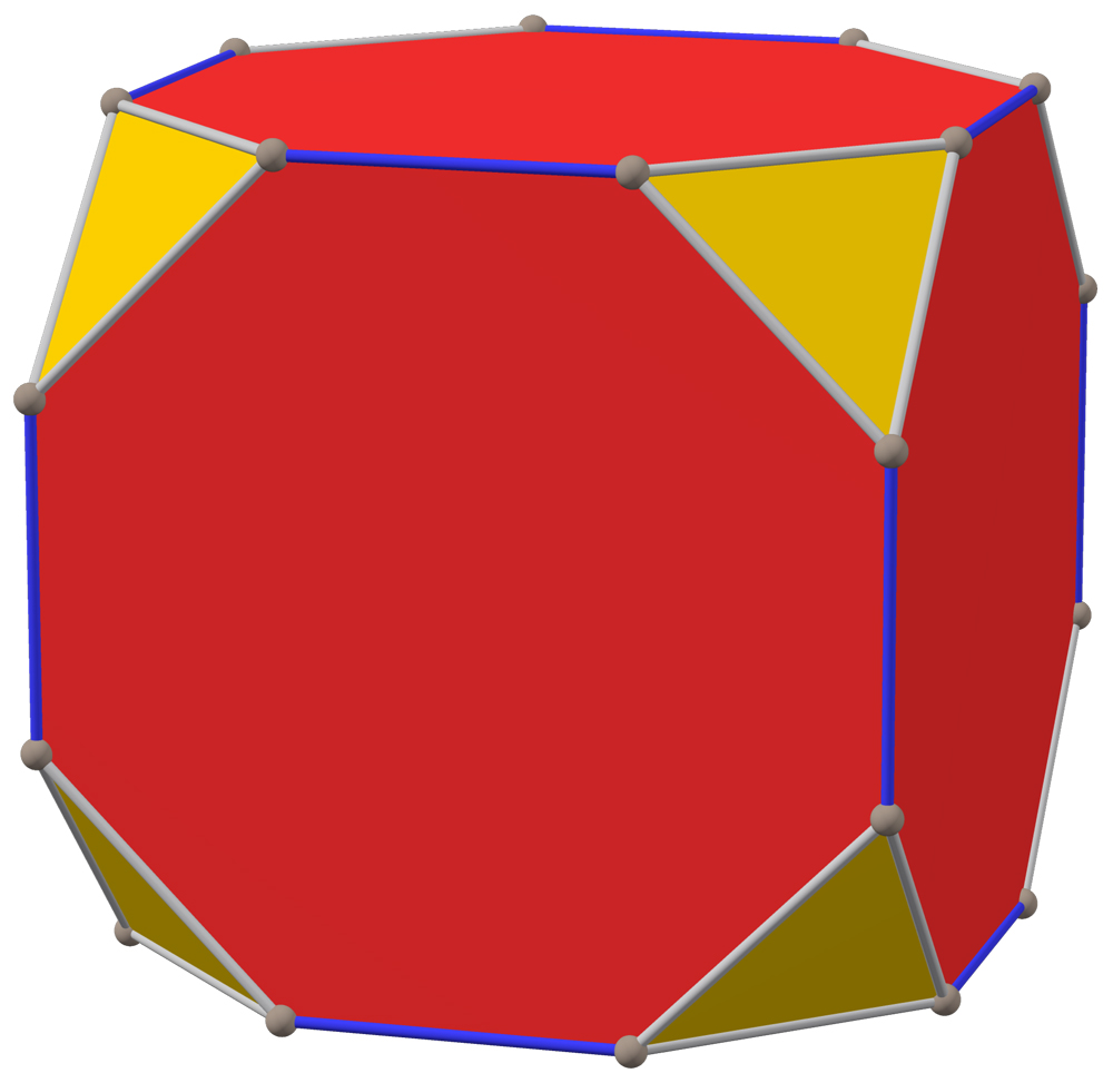
Figure 1: Truncated cube. [Image by Tilman Piesk, Wikipedia].

Tailoring differs from vertex truncation in two ways: first, it does not slice by a plane but instead uses a digon bound by a pair of equal-length geodesics (again, definition deferred), and second, rather than filling the hole with a new facet, the boundary of the hole is “sutured” closed without the addition of new surface.

Our first experiment started with a paper cube and tailored its $8$ vertices, producing the shape shown in Fig. 2.

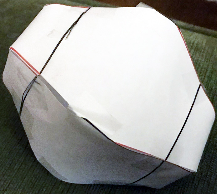
Figure 2: Cube after tailoring $8$ vertices.

Although not evident from this crude model, this shape is actually a convex polyhedron of $16$ vertices, an implication of Alexandrov’s Gluing Theorem. This led us imagine that continuing the process on the $16$ vertices might allow reshaping the cube into a roughly spherical polyhedron—“whittling” a cube to a sphere. And indeed, one of our main theorems is that any $P$ can be reshaped to any $Q\subset P$ by a finite sequence of tailorings (Theorem 4.6). This holds whether $Q$ has fewer vertices than $P$ or more vertices than $P$: see Fig. 3.

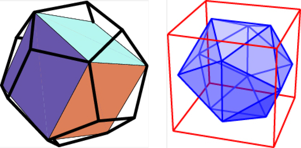
Figure 3: Cube inside dodecahedron. Icosahedron inside cube.

Investigating tailoring in Part I uncovered previously unexplored topics, including a notion of “unfolding” $Q$ onto $P$—cutting up $Q$ into pieces pasted non-overlapping onto $P$, and continuously folding $P$ onto $Q$. This led us to a systematic study of vertex-merging, a technique introduced by Alexandrov that can be viewed as a type of inverse operation to tailoring, a study we carry out in Part II. Here we start with $P$ and gradually enlarge it via vertex-merges until $P$ is embedded onto a nearly flat shape $S$: a doubly-covered triangle, an isosceles tetrahedron, a pair of cones, or a cylinder. The first two “vertex-merge irreducible shapes” (doubly-covered triangle or isosceles tetrahedron) are the result of vertex-merging in arbitrary order, and can result in disconnecting an $n$-vertex $P$ into $O(n^{2})$ pieces (Corollary 11.2). In contrast we pursue the goal of minimizing the disconnection of $P$, with the ultimate goal of achieving a planar net for $P$—a nonoverlapping simple polygon.

Toward this end, we partition $P$ into two half-surfaces by a quasigeodesic $Q$, a simple closed curve on $P$, convex to both sides. Then we can prove that a particular spiral vertex-merge sequence avoids disconnecting $P$ in each half. (Theorems 15.7 and 15.14.) This approach requires a notion of convexity and convex hull on the surface of a convex polyhedron, apparently novel topics, explored in our longest chapter, Chapter 13.

We can achieve a net for $P$ (Theorem 16.5) assuming the truth of a conjecture concerning quasigeodesics (Open Problem 18.14). This is among the many avenues for future work uncovered by our investigations.

Acknowledgements

We benefitted from discussions with Jin-ichi Itoh and with Anna Lubiw, on some topics of this work.

Costin Vîlcu’s research was partially supported by UEFISCDI, project no. PN-III-P4-ID-PCE-2020-0794.

Part I Tailoring for Every Body

Chapter 1 Introduction to Part I

Let $P$ and $Q$ be convex polyhedra, each the convex hull of finitely many points in ${\mathbb{R}^{3}}$. If $Q\subset P$, it is easy to see that $Q$ can be sculpted from $P$ by “slicing $P$ with planes.” By this we mean intersecting $P$ with half-spaces each of whose plane boundary contains a face of $Q$. If $Q\not\subset P$, we can shrink $Q$ until it fits inside. So a homothet of any given $Q$ can be sculpted from any given $P$, where a homothet is a copy possibly scaled, rotated, and translated. Main results of Part I are similar claims but via “tailorings”: a homothet of any given $Q$ can be tailored from any given $P$ (Theorems 4.6, 7.5, 8.1).

With some abuse of notation, we will use the same symbol $P$ for a polyhedral hull and its boundary. We define two types of tailoring. A digon-tailoring cuts off a single vertex of $P$ along a digon, and then sutures the digon closed. A digon is a subset $D(x,y)$ of $P$ bounded by two equal-length geodesic segments that share endpoints $x$ and $y$. A geodesic segment is a shortest geodesic between its endpoints. A crest-tailoring cuts off a single vertex of $P$ but via a more complicated shape we call a “crest.” Again the hole is sutured closed. We defer discussion of crests to Chapter 7. Meanwhile, we often shorten “digon-tailoring” to simply tailoring.

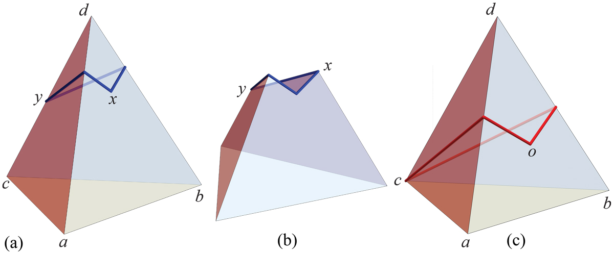
Figure 1.1: (a) A digon $D(x,y)$ on the regular tetrahedron $P=abcd$, surrounding vertex $d$. (b) Digon excised. (c) A digon $D(o,c)$ with one endpoint at vertex $c$, the other the centroid $o$.

Cutting out a digon means excising the portion of the surface between the geodesics, including the vertex they surround. Once removed, the digon hole is closed by naturally identifying the two geodesics along their lengths. This identification is often called “gluing” in the literature, although we also call it “zipping” or “suturing” or “sealing.” Fig. 1.1 illustrates digons on a regular tetrahedron $P$. In (a) of the figure, neither digon endpoint $x$ nor $y$ is a vertex of $P$; (b) shows $P$ after excision but before sealing. After sealing, both $x$ and $y$ become vertices. (See ahead to Fig. 2.6 for a depiction of the polyhedron that results after sealing.) In (c), one endpoint of the digon coincides with a vertex. Here, after excision and suturing, $o$ becomes a vertex and $c$ remains a vertex (of sharper curvature).

1.1 Alexandrov’s Gluing Theorem

Throughout, we make extensive use of Alexandrov’s Gluing Theorem [Ale05, p.100], which guarantees that the surface obtained after a tailoring of $P$ corresponds uniquely to a convex polyhedron $P^{\prime}$. A precise statement of this theorem, which we will abbreviate to AGT, is as follows.

Theorem AGT.

Let $S$ be a topological sphere obtained by gluing planar polygons (i.e., naturally identifying pairs of sides of the same length) such that at most $2\pi$ surface angle is glued at any point. Then $S$, endowed with the intrinsic metric induced by the distance in ${\mathbb{R}^{2}}$, is isometric to a convex polyhedron $P\subset{\mathbb{R}^{3}}$, possibly degenerated to a doubly-covered convex polygon. Moreover, $P$ is unique up to rigid motion and reflection in ${\mathbb{R}^{3}}$.

The case of doubly-covered convex polygon is important and we will encountered it often.

Because the sides of the digon are geodesics, gluing them together to seal the hole leaves $2\pi$ angle at all but the digon endpoints. The endpoints lose surface angle with the excision, and so have strictly less than $2\pi$ angle surrounding them. So AGT applies and yields a new convex polyhedron.

This shows that tailoring is possible and alters the given $P$ to another convex polyhedron. How to “aim” the tailoring toward a given target $Q$ is a long story, told in subsequent sections.

Alexandrov’s proof of his celebrated theorem is a difficult existence proof and gives little hint of the structure of the polyhedron guaranteed by the theorem. And as-yet there is no effective procedure to construct the three-dimensional shape of the polyhedron guaranteed by his theorem. It has only been established that there is a theoretical pseudopolynomial-time algorithm [KPD09], achieved via an approximate numerical solution to the differential equation established by Bobenko and Izmestiev [BI08] [O’R07]. But this remains impractical in practice. Only small or highly symmetric examples can be reconstructed, for example [ADO03] for the foldings of a square, and more recently [ALZ20] for polyhedra built from regular pentagons. Figs. 1.3 and 2.6 (ahead) were reconstructed through ad hoc methods.

AGT is a fundamental tool in the geometry of convex surfaces and, at a theoretical level, our work helps to elucidate its implications. While AGT has proved useful in several investigations, our application here to reshaping has, to our knowledge, not been considered before as the central object of study.

1.2 Tailoring Examples

Before discussing background context, we present several examples. Throughout we let $xy$ denote the line segment between points $x$ and $y$, $x,y\in{\mathbb{R}^{3}}$. Also we make extensive use of vertex curvature. The discrete (or singular) curvature ${\omega}(v)$ at a vertex $v\in P$ is the angle deficit: $2\pi$ minus the sum of the face angles incident to $v$.

Example 1.1.

Let $T=abcd$ be a regular tetrahedron, and let $o$ be the center of the face $abd$; see Fig. 1.1(c). Cut out the digon on $T$ between $c$ and $o$ “encircling” $d$, and zip it closed.

The unfolding $U(T)$ of $T$ with respect to $c$ is a planar regular triangle $c_{a}c_{b}c_{d}$ with center $o$. Cutting out that digon from $T$ is equivalent to removing from $T$ the isosceles triangle $oc_{a}c_{b}$. See Fig. 1.2(a). We zip it closed by identifying the digon-segments $c_{a}o$ and $c_{b}o$, and refolding the remainder of $T$ by re-identifying $c_{a}b$ and $bc_{d}$, and $c_{b}a$ and $ac_{d}$. The result is the doubly-covered kite $K=aobc_{d}$, shown in Fig. 1.2(b).

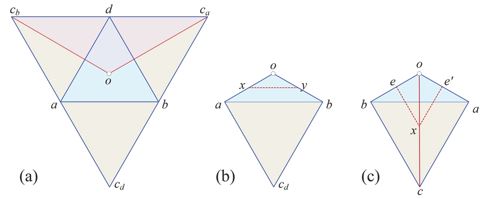
Figure 1.2: Illustrations for Examples 1.1–1.2. In (c), $e$ and $e^{\prime}$ are joined when the $D(x,y)$ digon is excised.

Example 1.2.

We further tailor the doubly-covered kite $K$ obtained in Example 1.1. Excising a digon encircling $o$, between points $x\in oa$ and $y\in ob$, and zipping closed, yields a doubly-covered pentagon, as in Fig. 1.2 (b).

If instead we excise a digon encircling $o$, between corresponding points $x,y\in oc$ on different sides of $K$ (see Fig. 1.2 (c)), and seal closed, the result is a non-degenerate pentahedron, illustrated in Fig. 1.3. This is among the rare cases where the polyhedron guaranteed by AGT can be explicitly reconstructed.

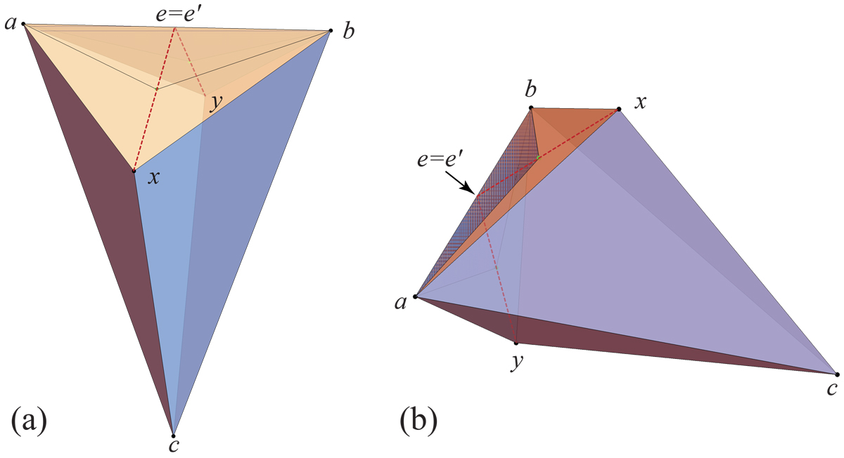
Figure 1.3: The non-degenerate pentahedron obtained in Example 1.2. The point marked $e=e^{\prime}$ is the join of the points $e$ and $e^{\prime}$ in Fig. 1.2(c), the midpoint of the edge $ab$.

Example 1.3.

A digon may well contain several vertices, but for our digon-tailoring we only consider those containing at most one vertex. The limit case of a digon containing no vertex is an edge between two vertices. (This will play a role in Chapter 8.) In this case, gluing back along the cut would produce the original polyhedron, but we can as well seal the cut closed from another starting point. For example, cutting along an edge of an isosceles tetrahedron (a polyhedron composed of four congruent faces) and carefully choosing the gluing leads to a doubly-covered rectangle. See Fig. 1.4.

By AGT, this limit-case tailoring of an empty-interior digon only applies between vertices $v_{1},v_{2}$ of curvatures ${\omega}_{1},{\omega}_{2}\geq\pi$, because both $v_{1}$ and $v_{2}$ will be identified with interior points of the edge.

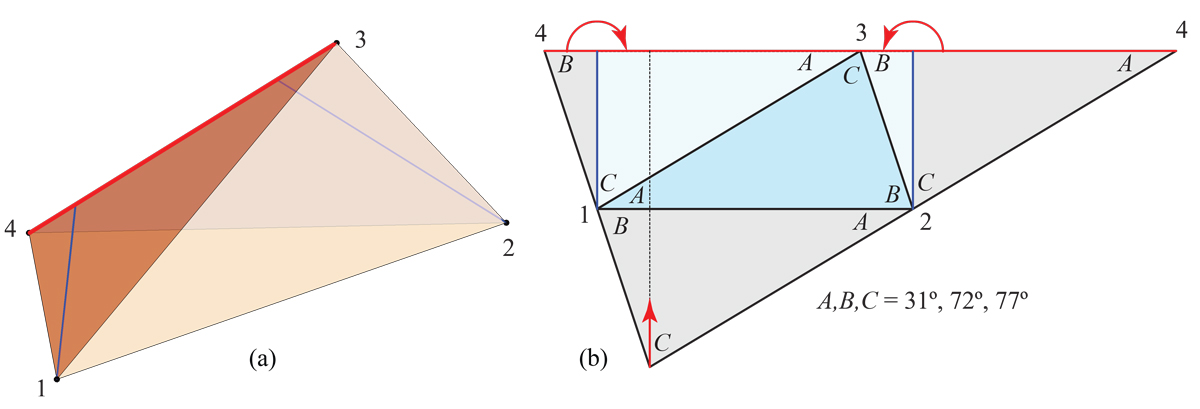
Figure 1.4: (a) An isosceles tetrahedron: All four faces are congruent. Cutting along $v_{3}v_{4}$ and regluing the two halves of that slit differently, creasing at the blue segments, yields a doubly-covered rectangle, as shown in (b), folding as shown.

In view of Fig. 1.2(c) and Fig. 1.3, it is clear that, even though tailoring is area decreasing, it is not necessarily volume decreasing.

Let a tailoring step remove vertex $v$ inside digon $D=(x,y)$. In general, neither $x$ nor $y$ is a vertex before tailoring, but they become vertices after removing $D$, thereby increasing the number of vertices of $P$ by $1$. This is illustrated in Fig. 1.1(ab). If one of $x$ or $y$ is a vertex and the other not, then the total number of vertices remains fixed, as in Fig. 1.1(c). And if both $x$ and $y$ are vertices, then the number of vertices of $P$ is decreased by $1$. The challenge answered in our work is to direct tailoring to “aim” from one polyhedon $P$ to the target $Q$, which may have a quite different number of vertices.

1.3 Summary of Part-I Results

Here we list our main theorems in Part I, each with a succinct (and at this stage, quite approximate) summary of their claims.

• Theorem 4.6: $Q$ may be digon-tailored from $P$, tracking a sculpting of $P$ to $Q$.

• Theorem 7.5: $P$ may be crest-tailored to $Q$, again tracking a sculpting.

• Theorem 8.1: A different proof of a similar result, that $P$ may be digon-tailored to a homothet of $Q$, but this time without relying on sculpting.

• Theorems 6.2 and 7.5 and 8.3: Tailoring algorithms have time-complexity $O(n^{4})$.

• Theorem 9.1: Reversing tailoring yields procedures for enlarging $Q$ inside $P$ to match $P$. As a consequence, $Q$ may be cut up and “unfolded” isometrically onto $P$.

Along the way to our central theorems, we obtain results not directly related to AGT:

• Theorem 2.9: If two convex polyhedra with the same number of vertices match on all but the neighborhoods of one vertex, then they are congruent.

• Theorem 3.2: Every “g-dome” can be partitioned into a finite sequence of pyramids by planes through its base edges.

The above results raise several open problems of various natures, either scattered along the text or presented in the last section of Part I.

Finally, we sketch the logic behind the first result listed above, whose statement in Chapter 4 we repeat here:

Theorem 4.6.

Let $P$ be a convex polyhedron, and $Q\subset P$ a convex polyhedron resulting from repeated slicing of $P$ with planes. Then $Q$ can also be obtained from $P$ by tailoring. Consequently, for any given convex polyhedra $P$ and $Q$, one can tailor $P$ “via sculpting” to obtain any homothetic copy of $Q$ inside $P$.

Start with $Q$ inside $P$, and imagine a sequence of slices by planes that sculpt $P$ to $Q$. Lemma 4.4 shows how to digon-tailor one such slice, which then establishes the claim that we can tailor $P$ to $Q$. Theorem 4.6 is achieved by first slicing off shapes we call “g-domes,” and then showing in Theorem 3.2 that every g-dome can be reduced to its base by slicing off pyramids, i.e., by vertex truncations. Lemma 4.4 shows that such vertex truncations can be achieved by tailoring. And the proof of Lemma 4.4 relies on the rigidity established by Theorem 2.9. So the path of logic is:

$$\textrm{plane slice}\;\to\;\textrm{g-domes}\;\to\;\textrm{pyramids}\;\to\; \textrm{digon removals}\;.$$

$$\uparrow$$

rigidity

Chapter 2 Preliminaries

In this chapter we present basic properties of cut loci on convex polyhedra, the star-unfolding, prove a rigidity result, and describe the technique of vertex-merging. All of these geometric tools will be needed subsequently. The reader might skip this section and return to it as the tools are deployed.

2.1 Cut locus properties

The cut locus $C(x)$ of the point $x$ on a convex polyhedron $P$ is the closure of the set of points to which there is more than one shortest path from $x$. This concept goes back to Poincaré [Poi05], and has been studied algorithmically since [SS86] (there, the cut locus is called the “ridge tree”). The cut locus is one of our main tools throughout this work. The next lemma establishes notation and lists several known properties.

Lemma 2.1 (Cut Locus Basics).

The following hold for the cut locus $C(x)$:

1. $C(x)$ has the structure of a finite $1$-dimensional simplicial complex which is a tree. Its leaves (endpoints) are vertices of $P$, and all vertices of $P$, excepting $x$ (if it is a vertex) are included in $C(x)$. All points interior to $C(x)$ of tree-degree $3$ or more are known as ramification points of $C(x)$. All vertices of $P$ interior to $C(x)$ are also considered as ramification points.

2. Each point $y$ in $C(x)$ is joined to $x$ by as many geodesic segments as the number of connected components of $C(x)\setminus{y}$. For ramification points in $C(x)$, this is precisely their degree in the tree.

3. The edges of $C(x)$ are geodesic segments on $P$.

4. Assume the geodesic segments ${\gamma}$ and ${\gamma}^{\prime}$ (possibly ${\gamma}={\gamma}^{\prime}$) from $x$ to $y\in C(x)$ are bounding a domain $D$ of $P$, which intersects no other geodesic segment from $x$ to $y$. Then there is an arc of $C(x)$ at $y$ which intersects $D$ and it bisects the angle of $D$ at $y$.

Proof.

The statements (i)-(ii) and (iv) are well known. The statement (iii) is Lemma 2.4 in [AAOS97]. ∎

The following is Lemma 4 in [INV12].

Lemma 2.2 (Path Cut Locus).

If $C(x)$ is a path, the polyhedron is a doubly-covered (flat) convex polygon, with $x$ on the rim.

The following lemma will be invoked in Chapter 5.

Lemma 2.3 (Angle $<\pi$).

Let $x$ be a point on a convex polyhedron $P$ and let $y$ be a ramification point of $C(x)$ of degree $k\geq 2$. Let $e_{1},...,e_{k}$ be the edges of $C(x)$ incident to $y$, ordered counterclockwise, and let ${\alpha}_{j}$ be the angle of the sector between $e_{j}$ and $e_{j+1}$ at $y$ (with $k+1\equiv 1$). Then ${\alpha}_{j}<\pi$, for all $j=1,...,k$.

Proof.

Let ${\gamma}_{1},...{\gamma}_{k}$ be the geodesic segments from $x$ to $y$, say with ${\gamma}_{j}$ between $e_{j}$ and $e_{j+1}$ (again with $k+1\equiv 1$). See Fig. 2.1. By Lemma 2.1 (iv), $e_{j}$ is the bisector of $\angle({\gamma}_{j},{\gamma}_{j+1})$. Put $2{\beta}_{j+1}=\angle({\gamma}_{j},{\gamma}_{j+1})$. Then the total surface angle ${\theta}_{y}$ incident to $y$ satisfies ${\theta}_{y}=\sum_{j=1}^{k}2{\beta}_{j}\leq 2\pi$ if $k\geq 3$, and ${\theta}_{y}<2\pi$ if $k=2$. Therefore, when $k\geq 3$, $\sum_{j=1}^{k}{\beta}_{j}=\pi$ and so ${\alpha}_{j}={\beta}_{j}+{\beta}_{j+1}<\pi$. And when $k=2$, ${\alpha}_{1}={\alpha}_{2}={\beta}_{1}+{\beta}_{2}<\pi$. ∎

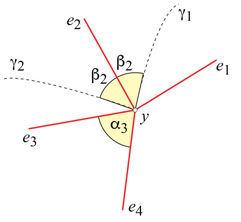
Figure 2.1: Edge $e_{2}$ of $C(x)$ bisects $\angle({\gamma}_{1},{\gamma}_{2})=2{\beta}_{2}$.

2.1.1 Star-Unfolding and Cut Locus

Next we introduce a general method for unfolding any convex polyhedron $P$ to a simple (non-overlapping) polygon in the plane. We use this subsequently largely because of its connection to the cut locus.

To form the star-unfolding of a $P$ with respect to $x$, one cuts $P$ along the geodesic segments (unique if $x$ is “generic”) from $x$ to every vertex of $P$. The idea goes back to Alexandrov [Ale05]; the non-overlapping of the unfolding was established in [AO92], where the next result was also proved. See Fig. 2.2.

Lemma 2.4 ($S_{P}$ Voronoi Diagram).

Let $S_{P}=S_{P}(x)$ denote the star-unfolding of $P$ with respect to $x\in P$. Then the image of $C(x)$ in $S_{P}$ is the restriction to $S_{P}$ of the Voronoi diagram of the images of $x$.

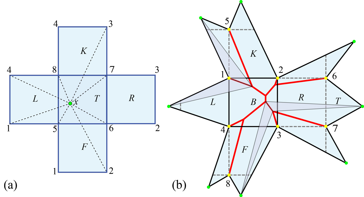
Figure 2.2: (a) Cut segments to the $8$ vertices of a cube from a point $x$ on the top face. (No cut is interior to the bottom face.) T, F, R, K, L, B $=$ Top, Front, Right, Back, Left, Bottom. (b) The star-unfolding from $x$. The cut locus $C(x)$ (red) is the Voronoi diagram of the $8$ images of $x$ (green). Two pairs of fundamental triangles are shaded.

Notice that several properties of cut loci, presented in the previous section, could easily be derived from Lemma 2.4.

2.1.2 Fundamental Triangles

A geodesic triangle on $P$ (i.e., with geodesic segments as sides) is called flat if its curvature vanishes.

Lemma 2.5 (Fundamental Triangles [INV12]).

For any point $x\in P$, $P$ can be partitioned into flat triangles whose bases are edges of $C(x)$, and whose lateral edges are geodesic segments from $x$ to the ramification points or leaves of $C(x)$. Moreover, those triangles are isometric to plane triangles, congruent by pairs.

See Fig. 2.2(b) (and ahead to Fig. 8.1).

2.1.3 Cut Locus Partition

Another tool we need (in Chapter 4) is a cut locus partition lemma, a generalization of lemmas in [INV12]. On a polyhedron $P$, connect a point $x$ to a point $y\in C(x)$ by two geodesic segments ${\gamma},{\gamma}^{\prime}$. This partitions $P$ into two “half-surface” digons $H_{1}$ and $H_{2}$. If we now zip each digon separately closed by joining ${\gamma}$ and ${\gamma}^{\prime}$, AGT leads to two convex polyhedra $P_{1}$ and $P_{2}$. The lemma says that the cut locus on $P$ is the “join” of the cut loci on $P_{i}$. See Fig. 2.3.

Lemma 2.6 (Cut Locus Partition).

Under the above circumstances, the cut locus $C(x,P)$ of $x$ on $P$ is the join of the cut loci on $P_{i}$: $C(x,P)=C(x,P_{1})\sqcup_{y}C(x,P_{2})$, where $\sqcup_{y}$ joins the two cut loci at point $y$. And starting instead from $P_{1}$ and $P_{2}$, the natural converse holds as well.

Proof.

Notice first that a straightforward induction and Lemma 2.5 on fundamental triangles shows that the cut locus of $x$ on $P_{i}$ is indeed the truncation of $C(x,P)$. Therefore, $C(x,P)=C(x,P_{1})\sqcup_{y}C(x,P_{2})$.

Assume we start now from $P_{1}$ and $P_{2}$, having vertices $x_{1},y_{1}\in P_{1}$ and $x_{2},y_{2}\in P_{2}$ such that

• ${\rho}_{P_{1}}(x_{1},y_{1})={\rho}_{P_{2}}(x_{2},y_{2})$, where ${\rho}_{P_{i}}(\;)$ is the geodesic distance between the indicated points on $P_{i}$.

• ${\theta}_{x_{1}}+{\theta}_{x_{2}}\leq 2\pi$, where ${\theta}_{x}$ is the total surface angle incident to $x$, and

• ${\theta}_{y_{1}}+{\theta}_{y_{2}}\leq 2\pi$.

Then we can cut open $P_{i}$ along a geodesic segment ${\gamma}_{i}$ from $x_{i}$ to $y_{i}$, $i=1,2$, and join the the two halves by AGT, such that $x_{1},x_{2}$ have a common image $x$, and $y_{1},y_{2}$ have a common image $y$.

Now, all geodesic segments starting at $x$ into $H_{i}$ remain in $H_{i}$, because geodesic segments do not branch. Therefore, $H_{1}$ has no influence on $C(x,P_{2})$ and $H_{2}$ has no influence on $C(x,P_{1})$. ∎

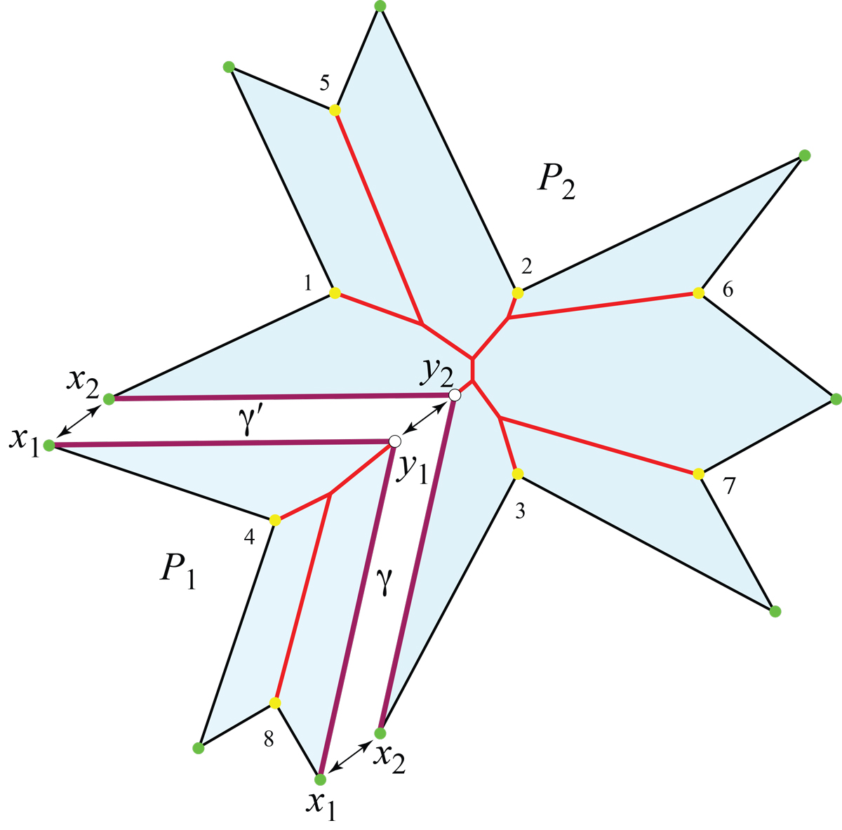
Figure 2.3: Geodesic segments ${\gamma}$ and ${\gamma}^{\prime}$ (purple) connect $x{=}x_{1}{=}x_{2}$ to $y{=}y_{1}{=}y_{2}$. $P_{1}$ folds to a tetrahedron, and $P_{2}$ to an $8$-vertex polyhedron, with $x$ and $y$ vertices in each. $P_{1}$ and $P_{2}$ are cut open along geodesic segments from $x_{i}$ to $y_{i}$ and glued together to form $P$. Based on the cube unfolding in Fig. 2.2(b).

2.2 Cauchy’s Arm Lemma

In several proofs, we will need an extension of Cauchy’s Arm Lemma, which we now describe.

Let $C=x_{1},\ldots,x_{n}$ be a directed polygonal chain in the plane, with left angles ${\theta}_{i}=\angle x_{i-1}x_{i}x_{i+1}$, where $x_{n}=x_{1}$ if $C$ is closed, and ${\theta}_{1}$ and ${\theta}_{n}$ undefined if $C$ is open. Let $d=|x_{1}x_{n}|$ be the distance between the endpoints, with $d=0$ if $C$ is closed. If ${\theta}_{i}\leq\pi$ for all $i$, then $C$ is a convex chain. Cauchy’s Arm Lemma applies to reconfiguration of $C$ while all the edge lengths remain fixed (the edges are bars). We use primes to indicate the reconfigured chain. The lemma says that if the ${\theta}_{i}$ angles are “straightened” while remaining convex, in the sense that ${\theta}_{i}\leq{\theta}^{\prime}_{i}\leq\pi$, then the distance $d^{\prime}=|x^{\prime}_{1}x^{\prime}_{n}|$ only increases: $d^{\prime}\geq d$.

For the extension needed later, we reformulate in terms of turn angles $\tau_{i}=\pi-{\theta}_{i}\geq 0$, as described in [O’R01]. Now the straightening condition says that $0\leq\tau^{\prime}_{i}\leq\tau_{i}$. The extended version of Cauchy’s arm lemma says that, as long as, in the reconfiguration, $-\tau_{i}\leq\tau^{\prime}_{i}\leq\tau_{i}$, then the same conclusion holds: $d^{\prime}\geq d$. Thus $C^{\prime}$ might no longer be a convex chain, but its reflexivities are bounded by the original turn angles. One way to interpret $d^{\prime}\geq d$ is that there is a “forbidden” disk of radius $d=|x_{1}x_{n}|$ centered on $x_{1}$ that $x^{\prime}_{n}$ cannot penetrate. See Fig. 2.4.

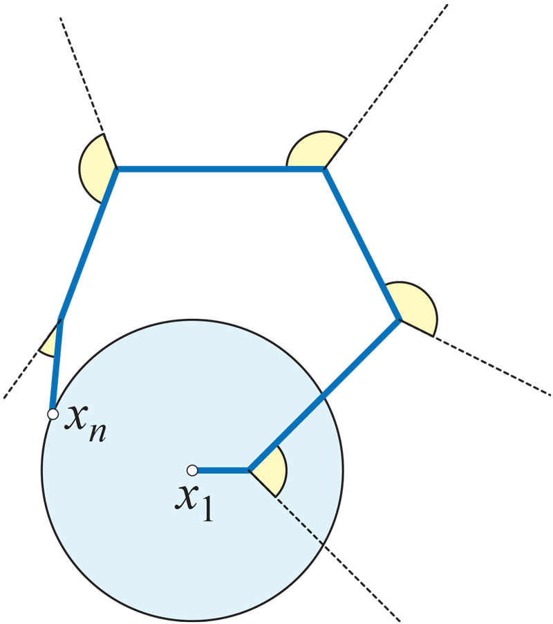
Figure 2.4: Any turns within the indicated $\pm\tau_{i}$ angle ranges constitute straightening. Then $x_{n}$ will not penetrate the $|x_{1}x_{n}|$ disk.

We summarize in a theorem:

Theorem 2.7.

(Cauchy’s Arm Lemma.) A straightening reconfiguration of a planar convex chain $C$—retaining edge-lengths fixed and confining new turn angles $\tau^{\prime}_{i}$ to lie in $[-\tau_{i},\tau_{i}]$—only increases the distance between the endpoints: $|x^{\prime}_{1}x^{\prime}_{n}|\geq|x_{1}x_{n}|$.

The next elementary result assures the angle increase, in the frameworks in which we will apply Cauchy’s Arm Lemma.

Lemma 2.8.

Consider three rays $r_{1},r_{2},r_{3}$ in ${\mathbb{R}}^{3}$, emanating from the point $w$, and put ${\tau}_{i}=\angle(r_{i},r_{i+1})$, with $3+1\equiv 1$ mod $3$. Then $\theta_{1}\leq\theta_{2}+\theta_{3}$.

Proof.

Imagine a unit sphere $S$ centered on $w$ and let $\{s_{i}\}=r_{i}\cap S$, and use ${\rho}$ to indicate spherical distance. Then the claim of the lemma is the triangle inequality for spherical distances: ${\rho}(s_{1},s_{2})\leq{\rho}(s_{1},s_{3})+{\rho}(s_{2},s_{3})$. ∎

2.3 A Rigidity Result

In this section we present a technical result for later use, which may be of independent interest. The theorem says that two convex polyhedra that are isometric on all but the neighborhoods of one vertex, are in fact congruent. We also show this result cannot be strengthened: two convex polyhedra can differ in the neighborhoods of just two vertices.

Theorem 2.9.

Assume $P,Q$ are convex polyhedra with the same number of vertices, such that there are vertices $p\in P$ and $q\in Q$, and respective small neighborhoods $N_{p}\subset P$, $N_{q}\subset Q$ not containing other vertices, and an isometry $\iota:P\setminus N_{p}\to Q\setminus N_{q}$. Then $P$ is congruent to $Q$.

Proof.

The existence of $\iota$ on all but neighborhoods of $p$ and $q$ yields, in particular, that the curvatures ${\omega}_{P}(p)$ of $P$ at $p$ and ${\omega}_{Q}(q)$ of $Q$ at $q$ are equal, to satisfy the curvature sum of $4\pi$ (by Gauss-Bonnet).

Take a point $x\in P$ joined to each vertex of $P$ by precisely one geodesic segment, a generic point $x$. Such an $x$ maybe be found in a “ridge-free” region of $P$ [AAOS97]; it is equivalent to the fact that no vertex of $P$ is interior to $C(x)$. Moreover, we may choose $x$ such that $\iota(x)$ has the same property on $Q$.

Denote by $u$ the ramification point of $C(x)$ neighboring $p$ in $C(x)$, i.e., the ramification point of degree $\geq 3$ closest to $p$. Let $v$ be the similar ramification point of $C(\iota(x))$ neighboring $q$ in $C(\iota(x))$. Since $N_{p}$ and $N_{q}$ are small, we may assume they are disjoint from $u$ and $v$ and all the segments described above.

Star unfold $P$ with respect to $x$, and $Q$ with respect to $\iota(x)$, and denote by $S_{P}$ and $S_{Q}$ the resulting planar polygons. We’ll continue to use the symbols $p$ and $q$, $u$ and $v$ to refer to the corresponding points in $S_{P}$ and $S_{Q}$ respectively. Let $x_{i}$, $i=1,2$ be the images of $x$ surrounding $p$ in $S_{P}$, and $\iota(x_{i})$ the similar images in $S_{Q}$. See Fig. 2.5(a,b).

By hypothesis, we have respective neighborhoods $\bar{N}_{p}\subset S_{P}$ and $\bar{N}_{q}\subset S_{Q}$ and an isometry $\bar{\iota}$ induced by $\iota$, with $\bar{\iota}:S_{P}\setminus\bar{N_{p}}\to S_{Q}\setminus\bar{N_{q}}$. Thus in Fig. 2.5(b), all of $S_{P}$ outside of the wedge $(x_{1},u,x_{2})$ is identical in $S_{Q}$. Therefore the triangles ${x}_{1}{u}{x}_{2}$ and ${x}^{\prime}_{1}{v}{x}^{\prime}_{2}$ are congruent. Moreover, ${p}$ lies on the bisector of the angle $\angle{x}_{1}{u}{x}_{2}$, and ${q}$ lies on the bisector of the angle $\angle{x}^{\prime}_{1}{v}{x}^{\prime}_{2}$. Since $\angle{x}_{1}{p}{u}=\angle{x}^{\prime}_{1}{q}{v}=\pi-\frac{1}{2}{\omega}(p)=\pi-\frac{1}{2}{\omega}(q)$, $p$ and $q$ are uniquely determined. Consequently, $S_{P}$ and $S_{Q}$ coincide, and refolding according to the same gluing identifications leads to congruent $P$ and $Q$. ∎

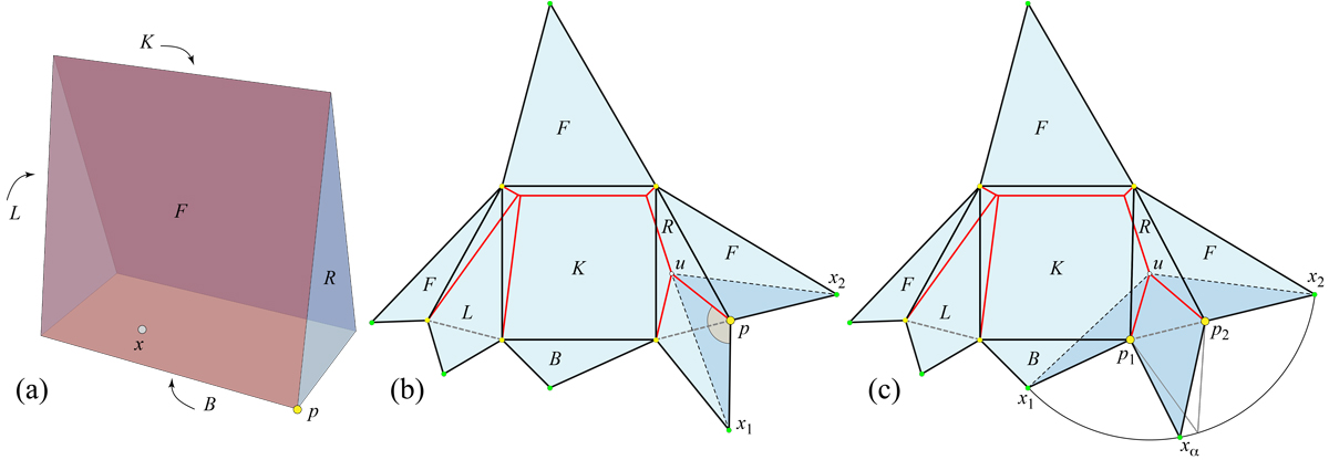
Figure 2.5: (a) A $6$-vertex polyhedron $P$. The $F$ and $K$ faces are unit squares; $B$ is a $1\times\frac{1}{2}$ rectangle, with $x\in B$. (b) Star-unfolding $S_{P}$ of $P$. $\angle{x}_{1}{p}{u}$ is marked. (c) Moving $x_{\alpha}$ on the circle arc moves the bisectors incident to $u$, and so moves $p_{1}$ and $p_{2}$. Refolding results in a polyhedron incongruent to (a).

Remark 2.10.

It is perhaps surprising that the above result cannot be extended to claim that isometries excluding neighborhoods of two vertices always imply congruence.

Proof.

If the points $p_{1},p_{2}\in P$ and $q_{1},q_{2}\in Q$ do not have a common neighbor in $C(x)$ and $C(\iota(x))$ respectively, the above proof establishes rigidity.

Next we focus on $P$, and try to find positions for $p_{1},p_{2}\in P$ determined by the hypotheses. Assume, in the following, that $p_{1},p_{2}\in P$ have a common degree-$3$ ramification neighbor $u$ in $C(x)$.

Star unfold $P$ with respect to some $x\in P$, to $S_{P}$. The region of $S_{P}$ exterior to the wedge $(x_{1},u,x_{2})$ is uniquely determined and identical in $S_{Q}$. See Fig. 2.5(c).

Take a point $x_{\alpha}$ on the circle of center ${u}$ and radius $|x_{1}u|=|x_{2}u|$. We now argue that positions of $x_{\alpha}$ on this circle allow $p_{1}$ and $p_{2}$ to vary while maintaining all outside of the $(x_{1},u,x_{2})$ wedge fixed.

Let $\angle{x}_{\alpha}{u}{x}_{1}=2{\alpha}$. On the bisector of that angle incident to $u$, one can uniquely determine a point ${p}_{1}$ such that $\angle{x}_{1}{{p_{1}}}{u}=\pi-\frac{1}{2}{\omega}(p_{1})$. Similarly, one can uniquely determine a point ${p}_{2}$ on the bisector of that angle $\angle{x}_{\alpha}{u}{x}_{2}$, such that $\angle{x}_{2}{{p_{2}}}{u}=\pi-\frac{1}{2}{\omega}(p_{2})$.

Thus we have identified a continuous $1$-parameter family of star-unfoldings, and consequently of convex polyhedra, verifying the hypotheses. ∎

2.4 Vertex-Merging

Digon-tailoring is, in some sense, the opposite of vertex-merging, a technique introduced by A. D. Alexandrov [Ale05, p. 240], and subsequently used later by others, see e.g. [Zal07], [OV14], [O’R20]. We will employ vertex-merging in Chapters 8 and 9, and focus on it in Part II.

Consider two vertices $v_{1},v_{2}$ of $P$ of curvatures ${\omega}_{1},{\omega}_{2}$, with ${\omega}_{1}+{\omega}_{2}<2\pi$, and cut $P$ along a geodesic segment ${\gamma}$ joining $v_{1}$ to $v_{2}$. Construct a planar triangle $T=\bar{v}^{\prime}\bar{v}_{1}\bar{v}_{2}$ of base length $|\bar{v}_{1}-\bar{v}_{2}|=|{\gamma}|$ and the base angles equal to ${\omega}_{1}/2$ and ${\omega}_{2}/2$ respectively. Glue two copies of $T$ along the corresponding lateral sides, and further glue the two bases of the copies to the two “banks” of the cut of $P$ along ${\gamma}$. By Alexandrov’s Gluing Theorem (AGT), the result is a convex polyhedral surface $P^{\prime}$. On $P^{\prime}$, the points (corresponding to) $v_{1}$ and $v_{2}$ are no longer vertices because exactly the angle deficit at each has been sutured-in; they have been replaced by a new vertex $v^{\prime}$ of curvature ${\omega}^{\prime}={\omega}_{1}+{\omega}_{2}$. So vertex-merging always reduces the number of vertices of $P$ by one. See Fig. 2.6.

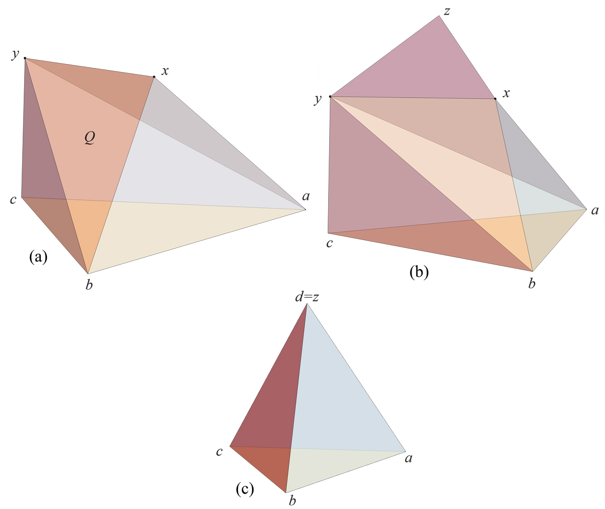
Figure 2.6: (a) $Q$ is a $5$-vertex, $6$-face polyhedron, symmetric about a vertical plane through $xy$. Its base $abc$ is an equilateral triangle. (b) Vertex merging $x$ and $y$ by gluing a pair of $xyz$ triangles. (c) The merging reduces $Q$ to a regular tetrahedron (not to same scale). Cf. Fig. 1.1(a,b).

In order to repeat vertex-merging, we need to know when there is a pair of vertices that can be merged. This is answered in the following lemma.

Lemma 2.11.

Every convex polyhedron $Q$ has at least one pair of vertices admitting merging, unless it is an isosceles tetrahedron or a doubly-covered triangle.

Recall from Chapter 1 that an isosceles tetrahedron $T$ is a tetrahedron with four congruent faces, and each vertex of curvature $\pi$. See Fig. 1.4.

Proof.

If there is a pair of vertices whose sum of curvatures is strictly less than $2\pi$, then vertex-merging is possible, as just described. So assume that, for any two vertices of $Q$, their sum of curvatures is at least $2\pi$. In this case, it must be that $n\leq 4$. Indeed, since $\sum_{v\in Q}{\omega}(v)=4\pi$ (by the Gauss-Bonnet theorem), if the sum of at least $5$ positive numbers is $4\pi$ then the smallest two have sum $<2\pi$.

If $n=3$, the cut locus of any vertex is a line-segment, by Lemma 2.1(i), so $Q$ is a doubly-covered triangle (see Lemma 2.2).

If $n=4$ then necessarily all vertex curvatures of $Q$ are $\pi$. Indeed, if the sum of $4$ positive numbers is $4\pi$ then the smallest two have the sum $\leq 2\pi$, with equality if and only if all are $\pi$. So $Q$ is an isosceles tetrahedron. ∎

Chapter 3 Domes and Pyramids

One of our goals in this work, achieved in Theorem 4.6, is to show that if $Q$ can be obtained from $P$ by sculpting, then it can also be obtained from $P$ by tailoring. A key step (Lemma 4.1) repeatedly slices off shapes we call g-domes. Each g-dome slice can itself be achieved by slicing off pyramids, i.e., by suitable vertex truncations. Lemma 4.4 will show that slicing off a pyramid can be achieved by tailoring, and thus leading to Theorem 4.6.

Our main goal in this chapter is to prove that g-domes can be partitioned into “stacked” pyramids, a crucial part of the above process. We illustrate the slice $\to$ g-domes and g-dome $\to$ pyramids of the process on a simple example, a tetrahedron $Q$ inside a cube $P$. Later (in Chapter 4) this example will be completed by tailoring the pyramids.

3.1 Domes

As usual, a pyramid $P$ is the convex hull of a convex polygon base $X$, and one vertex $v$, the apex of $P$, that does not lie in the plane of $X$. The degree of $v$ is the number of vertices of $X$.

A dome is a convex polyhedron $G$ with a distinguished face $X$, the base, and such that every other face of $G$ shares a (positive-length) edge with $X$. Domes have been studied primarily for their combinatorial [Epp20], [EL13] or unfolding [DO07] properties. In [Epp20] they are called “treetopes” because removing the base edges from the $1$-skeleton leaves a tree, which the author calls the canopy. Here we need a slight generalization.

A generalized-dome, or g-dome $G$, has a base $X$, with every other face of $G$ sharing either an edge or a vertex with $X$. Every dome is a g-dome, and it is easy to obtain every g-dome as the limit of domes. An example is shown in Fig. 3.1, which also shows that removing base edges from the $1$-skeleton does not necessarily leave a tree: $(v_{1},x_{2},v_{2})$ forms a cycle. Let us define the top-canopy $T$ of a g-dome $G$ as the graph that results by deleting from the $1$-skeleton of $G$ all base vertices and their incident edges. In Fig. 3.1 the top-canopy is $v_{1}v_{2}$.

Figure 3.1: A g-dome with base $\triangle x_{1}x_{2}x_{3}$ and top-canopy $v_{1}v_{2}$.

Lemma 3.1.

The top-canopy $T$ of a g-dome $G$ is a tree.

Proof.

If $G$ is a dome, the claim follows, because even including the edges incident to the base $X$ results in a tree, and removing those edges leaves a smaller tree.

If $G$ is not a dome, then slice it with a plane parallel to, and at small distance above, the base. The result is a dome, and we can apply the previous reasoning. ∎

3.2 Cube/Tetrahedron Example

In this section we start to track an example, tailoring a cube to a tetrahedron. $P$ is a triangulated unit cube. $Q$ is a right tetrahedron in the corner of $P$; see Fig. 3.2(a). $Q$ can be obtained from $P$ by a single slice by plane $\Pi=p_{1}p_{3}p_{8}$. The algorithm to be described in Chapter 6 will first produce two g-domes $G_{1}$ and $G_{2}$, and reducing those g-domes will lead to four pyramids $P_{1},P_{2},P_{3},P_{4}$. Later (in Chapter 4) we will show how each of those pyramids is reduced by digon-tailoring, finally yielding $Q$.

3.2.1 Slice $\to$ G-Domes for Cube/Tetrahedron

Now we describe at an intuitive level what will be proved in Lemma 4.1: that the slice by $\Pi$ can be effected by partitioning the sliced portion of $P$ into g-domes.

We start by rotating the plane $\Pi$ about the edge $p_{1}p_{3}$ until it encounters a face of $P$; call that plane $\Pi_{0}=p_{1}p_{2}p_{3}$. Now continue rotating until we reach $\Pi_{1}$ when (a) The portion of $P$ between $\Pi_{0}$ and $\Pi_{1}$ is a g-dome with base on $\Pi_{1}$, and (b) Any further rotation would render the portion between the planes to a polyhedron no longer a g-dome. $\Pi_{1}=p_{1}p_{3}p_{7}p_{5}$, because any further rotation would isolate the face $p_{5}p_{6}p_{7}$ of $P$, no longer touching $\Pi_{1}$. Note here the top face of the cube is triangulated with the diagonal $p_{5}p_{7}$. See Fig. 3.2(bc). Continuing to rotate, we reach the original $\Pi$, partitioning the g-dome illustrated in Fig. 3.2(d). So $G_{1}$ has base $X_{1}=p_{1}p_{3}p_{7}p_{5}$ and top-canopy $p_{2}p_{6}$, and $G_{2}$ has base $X_{2}=p_{1}p_{2}p_{3}$ and top-canopy $p_{5}p_{7}$. It is clear that removing $G_{1}\cup G_{2}$ would reduce $P$ to $Q$.

Figure 3.2: (a) $Q$ in corner of cube $P$. (b) Partitioning sliced portion of $P$ into two g-domes. (c,d) G-domes $G_{1}$ and $G_{2}$.

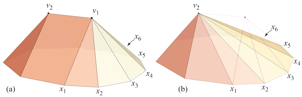
Figure 3.3: (a) A dome $G$. Vertex $v_{1}$ of degree $k_{1}=6$ is adjacent to $X$, i.e., there are edges $v_{1}x_{i}$. (b) $G^{\prime}$ after removal of $v_{1}$.

3.3 Proof: G-dome $\to$ Pyramids

We now prove the reduction of a g-dome to pyramids, using Fig. 3.3 to illustrate the proof details. Afterward we will return to the cube/tetrahedron example to apply the constructive proof to $G_{1}$ and $G_{2}$.

Theorem 3.2.

Every g-dome $G$ of base $X$ can be partitioned into a finite sequence of $n$ pyramids $P_{i}$ with the following properties:

• Each $P_{i}$ has a common edge with $X$.

• Each $G_{j}=G\setminus\bigcup_{i=1}^{j}P_{i}$ is a g-dome, for all $j=1,...,n$.

• The last pyramid $P_{n}$ in the sequence has the same base $X$ as $G$.

The partition into pyramids specified in this theorem has the special properties listed. Without these properties, it would be easier to prove that every g-dome may be partitioned into pyramids. But the properties are needed for the subsequent digon-tailoring described in Chapter 4. In particular, the pyramids are “stacked” in the sense that each can be sliced-off in sequence, with each slice retaining $X$ unaltered.

The proof is a double induction, and a bit intricate. One induction simply removes one vertex $v_{1}$ from the top-canopy. The second induction, inside the first one, reduces the degree of $v_{1}$ to achieve removal of $v_{1}$, at the cost of increasing the degree of $v_{2}$.

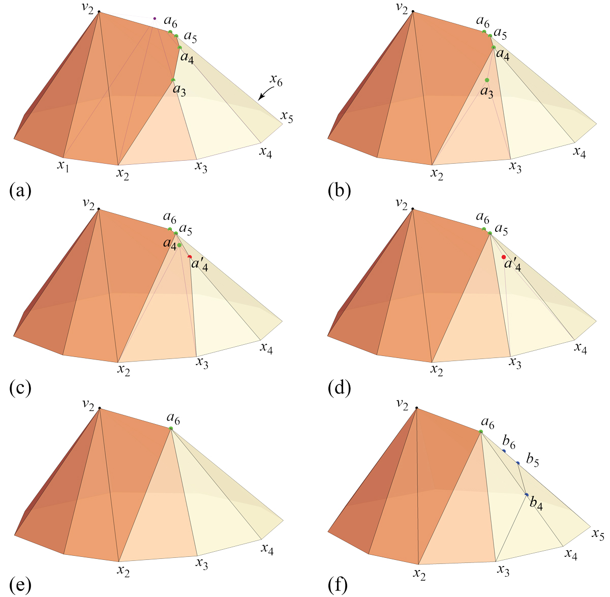
Figure 3.4: (a) After slicing by the plane $\Pi_{1}=x_{1}x_{2}v_{2}$. (b) Removing $a_{3}$. (c) Removing $a_{4}$ creates $a^{\prime}_{4}$. (d) Removing $a^{\prime}_{4}$. (e) $a_{6}$ has replaced $v_{1}$ with one lower degree. (f) Intersection points with $\Pi_{2}=x_{2}x_{3}v_{2}$.

Proof.

Let $m$ be the number of vertices in the top-canopy $T$ of $G$. If $m=1$, $G$ is already a pyramid, and we are finished. So assume $G$’s top-canopy $T$ has at least two vertices. Choose $v_{1}$ to be a leaf of $T$ given by Lemma 3.1, and $v_{2}$ its unique parent. Let $v_{1}$ be adjacent to $k$ vertices of $X$. If $G$ is a dome, $v_{1}$ has degree $k+1$; if $G$ is a g-dome, then possibly $v_{1}$ has degree $k+2$. Since the later case changes nothing in the proof, we assume for the simplicity of exposition that $G$ is a dome. Our goal is to remove $v_{1}$ through a series of pyramid subtractions.

Let the vertices of $X$ adjacent to $v_{1}$ be $x_{1},x_{2},\ldots,x_{k}$. Let $\Pi_{1}$ be the plane $x_{1}x_{2}v_{2}$. This plane cuts into $G$ under $v_{1}$, and intersects the edges $v_{1}x_{i}$, $i\geq 3$, in points $a_{i}$. In Fig. 3.4(a), those points are $a_{3},a_{4},a_{5},a_{6}$. Remove the pyramid whose apex is $v_{1}$ and whose base (in our example) is $x_{1},x_{2},a_{3},a_{4},a_{5},a_{6},v_{2}$.

We now proceed to reduce the chain of new vertices $a_{3},\ldots,a_{k}$ one-by-one until only $a_{k}$ remains.

First, with the plane $x_{2}x_{3}a_{4}$, we slice off the tetrahedron whose degree-$3$ apex is $a_{3}$; Fig. 3.4(b). Next, with the plane $x_{2}x_{3}a_{5}$, we slice off the pyramid with apex $a_{4}$. Unfortunately, because $a_{4}$ has degree-$4$, this introduces a new vertex $a^{\prime}_{4}$; Fig. 3.4(c). So next we slice with $x_{3}x_{4}a_{5}$ to remove the tetrahedron whose degree-$3$ apex is $a^{\prime}_{4}$; Fig. 3.4(d). Continuing in this manner, alternately removing a tetrahedron followed by a pyramid with a degree-$4$ apex, we reach Fig. 3.4(e).

Note that $v_{1}$ was connected to $k=6$ vertices of $X$, but $a_{6}$ is only connected to $5$: the connection of $v_{1}$ to $x_{1}$ has in a sense been transferred to $v_{2}$. In general, $a_{k}$ has degree one less than $v_{1}$’s degree, and the degree of $v_{2}$ has increased by $1$.

Now we repeat the process, starting by slicing with $\Pi_{2}=x_{2}x_{3}v_{2}$, which intersects the $a_{k}x_{i}$ edges at $b_{4},\ldots,b_{k}$. We remove the pyramid apexed at $a_{6}$ with base (in our example) of $x_{2},x_{3},b_{4},b_{5},b_{6},v_{2}$; Fig. 3.4(f). The same methodical technique will remove all but the last new vertex $b_{k}$, which replaces $a_{k}$ but has degree one smaller.

Continuing the process, slicing with $\Pi_{i}=x_{i}x_{i+1}v_{2}$, up to $i=k-1$, will lead to the complete removal of $v_{1}$, as previously illustrated in Fig. 3.3(b), completing the inner induction. Inverse induction on the number of vertices of the g-dome then completes the proof: each step reduces the number of top vertices by $1$, and the degree of $v_{2}$ increases by $k+1$, the degree lost at $v_{1}$.

With $G_{0}=G$, each $G_{j}$ is the intersection of $G_{k-1}$ with a closed half-space containing a base edge, so it is convex for all $j=1,...,n$. Indeed each $G_{j}$ is a g-dome, because all untouched faces continue to meet $X$ in either an edge or a vertex, and new faces always share an edge with $X$. ∎

The partition of a g-dome into pyramids given by Theorem 3.2 is not unique. For our example in Fig. 3.3(a), we finally get the pyramid apexed at $v_{2}$ in (b) of the figure, but we could as well have ended with a pyramid apexed at $v_{1}$.

We will see in Chapter 4 that one g-dome of $O(n)$ vertices reduces to $O(n^{2})$ pyramids of constant size, and $O(n)$ pyramids each of size $O(n)$.

3.3.1 G-domes $\to$ Pyramids for Cube/Tetrahedron

We now return to the cube/tetrahedron example, and show that following the proof of Theorem 3.2 partitions the two g-domes $G_{1}$ and $G_{2}$ into pyramids. We will see that the two g-domes partition into two pyramids each.

The analysis for $G_{1}$ is illustrated in Fig. 3.5. Note $G_{1}$ has been reoriented so that its base $X_{1}=p_{1}p_{3}p_{7}p_{5}$ is horizontal, and relabeled $x_{1}x_{2}x_{3}x_{4}$ to match the proof.

We proceed to describe each step, making comparisons to Figs. 3.3 and 3.4.

1. In (a) of the figure, the base of the g-dome has been oriented horizontally, and the correspondence between the cube labels and the labels used in the proof of Theorem 3.2 are shown. The top-canopy of $G_{1}$ is $v_{1}v_{2}$, with $v_{1}$ of degree-$5$ and $v_{2}$ of degree-$3$. Eventually $v_{1}$ will be removed and the degree of $v_{2}$ increased by $1$, as in Fig. 3.3.

2. The first step is to slice off a pyramid apexed at $v_{1}$ by the plane $x_{1}x_{2}v_{2}$. Due to the coplanar triangles, this has the effect of “erasing” the diagonal $x_{1}v_{1}$, as would have occurred if that diagonal had a dihedral angle different from $\pi$.

3. Next, the slice $x_{2}x_{3}v_{2}$ cuts off a pyramid $P_{1}$ apexed at $v_{1}$, a pyramid we will analyze in Section 4.4.1, leaving the shape in (d).

4. A new vertex $a_{3}$ is created by the slice in (c), with degree-$4$. This is the “replacement” for $v_{1}$ but of smaller degree. This corresponds to $a_{3}$ in Fig. 3.4(a), although here there are no further vertices $a_{4},\ldots$ along an $a$-chain.

5. We again slice with $x_{2}x_{3}v_{2}$, which reduces the degree of $a_{3}$ to $3$. This $a_{3}$ corresponds to $b_{4}$ in Fig. 3.4(f).

6. A final slice by $x_{3}x_{4}v_{2}$ removes $a_{3}$, leaving the pyramid $P_{2}$ shown. This completes the removal of $v_{1}$ in (a), increasing the degree of $v_{2}$ from $3$ to $4$. Because what remains is a pyramid, the processing stops.

So $G_{1}$ is partitioned into two pyramids, $P_{1}$ and $P_{2}$, apexed at $p_{2}$ and $p_{6}$ respectively.

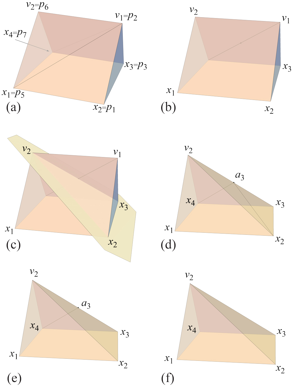
Figure 3.5: (a) g-dome $G_{1}$. (b) After slicing by $x_{1}x_{2}v_{2}$. (c,d) Slicing by $x_{2}x_{3}v_{2}$. (e,f) Two further slices remove $a_{3}$.

We perform a similar analysis for the simpler $G_{2}$, shown in Fig. 3.6, again reoriented so that its base $p_{8}p_{1}p_{3}$ is horizontal and relabeled $x_{1}x_{2}x_{3}$. Here the top-canopy is $v_{1}v_{2}$, and the first slice $x_{1}x_{2}v_{2}$ reduces $G_{2}$ to a pyramid $P_{2}$. So $G_{2}$ is also partitioned into two pyramids, $P_{3}$ and $P_{4}$, apexed at $p_{5}$ and $p_{7}$ respectively. Together $G_{1}$ and $G_{2}$ are partitioned into four pyramids.

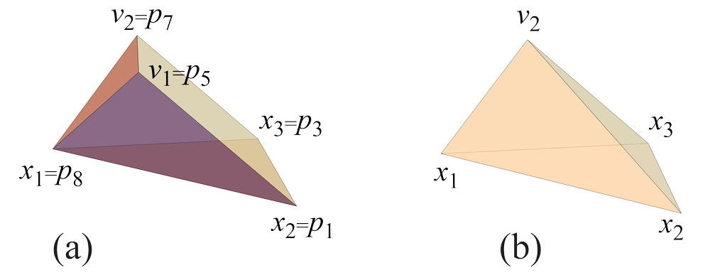
Figure 3.6: (a) $G_{2}$ with corresponding cube labels. (b) After slicing with $x_{1}x_{2}v_{2}$.

We will complete this example by tailoring the four pyramids in the next chapter.

Chapter 4 Tailoring via Sculpting

In this chapter we complete the proof that one slice of $P$ by plane $\Pi$ can be tailored to the face of $Q$ lying in $\Pi$, following the sequence slice $\to$ g-domes $\to$ pyramids $\to$ tailoring. The previous chapter established the g-domes $\to$ pyramids link. Here we first prove the relatively straightforward slice $\to$ g-domes process, and then concentrate on the more complex pyramid $\to$ tailoring step.

4.1 Slice $\to$ G-domes

Lemma 4.1.

With $Q\subset P$ and $\Pi$ a plane slicing $P$ and containing a face $F$ of $Q$, the sliced-off portion $P^{\prime}$ can be partitioned into a fan of $O(n)$ g-domes $G_{1},G_{2},\ldots$, a fan in the sense that the bases of the g-domes all share a common edge of $F$.

Figure 4.1: Dodecahedron sliced by $\Pi$. The polyhedron between each pair $\Pi_{i},\Pi_{i+1}$ is a g-dome.

Proof.

Assume $\Pi$ is horizontal, with $Q$ the portion below $\Pi$ and $P^{\prime}$ the portion above. Denote by $x_{i}$ the vertices of $Q$ in $\Pi$, $i=1,\ldots,m$; call the top face of $Q$ with these vertices $F$. Let $e$ be any edge of $F$, say $e=x_{1}x_{2}$, and let $F^{\prime}$ be the face of $Q$ sharing $e$ with $F$. Call the plane lying on $F^{\prime}$ $\Pi_{0}$.

Now imagine rotating $\Pi_{0}$ about $e$ toward $P^{\prime}$, noting as it passes through each vertex $v_{1},v_{2},\ldots$ in that order. For perhaps several consecutive vertices, the portion of $P^{\prime}$ between the previous and the current plane is a g-dome, but rotating further takes it beyond a g-dome. More precisely, let $\Pi_{1}$ through $v_{j_{1}}$ be the plane such that, in the sequence

$$v_{1},v_{2},\ldots,v_{j_{1}},v_{j_{1}+1},\ldots,v_{j_{2}},v_{j_{2}+1}\ldots\;,$$

the portion $G_{1}$ of $P^{\prime}$ between $\Pi_{0}$ and $\Pi_{1}$, including the vertices $v_{1},v_{2},\ldots,v_{j_{1}}$, is a g-dome based on $\Pi_{1}$, but the portion rotating further to include one more vertex, $v_{j_{1}+1}$, is not a g-dome. $\Pi_{2}$ through $v_{j_{2}}$ is defined similarly: the portion $G_{2}$ between $\Pi_{1}$ and $\Pi_{2}$ including $v_{j_{1}+1},\ldots,v_{j_{2}}$ is a g-dome based on $\Pi_{2}$, but including $v_{j_{2}+1}$ it ceases to be a g-dome. Here for each $\Pi_{i},\Pi_{i+1}$ pair, the base $X$ of the g-dome lies in $\Pi_{i+1}$.

Fig. 4.1 illustrates the process. Here $\Pi_{1}$ is through $v_{1}=v_{j_{1}}$, and the last g-dome lies between $\Pi_{3}$ and $\Pi$.

So we have now partitioned $P^{\prime}$ into g-domes $G_{1},G_{2},\ldots$. ∎

We will invoke Lemma 4.4 (ahead) to reduce each g-dome to its base by tailoring, in the order $G_{1},G_{2},\ldots$. This will reduce $P^{\prime}$ to just the top face $F$ of $Q$.

Having established the claim of the lemma for one slice, it immediately follows that it holds for an arbitrary number of slices. This was already illustrated in the cube/tetrahedron example in Chapter 3, and we will use it again in Theorem 4.6.

We should note that it is at least conceivable that only a single g-dome is needed above. See Open Problem 18.2.

4.2 Pyramid $\to$ Tailoring

The goal of this section is to prove that removal of a pyramid, i.e., a vertex truncation, can be achieved by (digon-)tailoring. We reach this in Lemma 4.4: a degree-$k$ pyramid $P$ can be removed by $k-1$ tailoring steps, each step excising one vertex by removal of and then sealing a digon. The first $k-2$ of these digons each have one endpoint a vertex, and so leave the total number of vertices of $P$ at $k+1$. The $(k-1)$-st digon has both endpoints vertices, and so its removal reduces the number of vertices to the $k$ base vertices.

We start with Lemma 4.2 which claims the result but only under the assumption that the slice plane is close to the removed vertex. Although this lemma is eventually superseded, it establishes the notation and the main idea. Following that, Lemma 4.3 removes the “sufficiently small” assumption of Lemma 4.2, but in the special case of $P$ a pyramid. Finally we reach the main claim in Lemma 4.4, which shows this special case encompasses the general case.

In the following, we use $\partial S$ to indicate the $1$-dimensional boundary of a $2$-dimensional surface patch $S$.

4.2.1 Notation

To help keep track of the notation throughout this critical section, we list the main symbols below.

• Initially $P$ and $Q$ are polyhedra with $Q\subset P$, with $P$ sliced by plane $\Pi$ to truncate vertex $v$ of degree $k$.

• Later we specialize $P$ to be the pyramid sliced off.

• $X=\Pi\cap P$ is the base of the pyramid, with vertices $\partial X=x_{1}x_{2}\ldots x_{k}$.

• The lateral faces of $P$ are denoted by $L$, so $P=X\cup L$.

• $D(x_{i},y_{i})$ is a digon with endpoints $x_{i}\in\partial X$ and $y_{i}$.

• $P_{j}$ is the modified pyramid after $j$ digon removals.

• $C(x_{i},P_{j})$ is the cut locus $C(x_{i})$ on $P_{j}$.

• The first ramification point of $C(x_{i},P_{j})$ beyond $y_{i}$ is $a_{i}$.

Notation will be repeated and supplemented within each proof.

4.3 Small volume slices

Lemma 4.2.

Let $P$ be a convex polyhedron, and $Q$ the result obtained by slicing $P$ with a plane $\Pi$ at sufficiently small distance to a vertex $v$ of $P$, and removing precisely that vertex. Then $Q$ can be obtained from $P$ by $k-1$ tailoring steps.

Proof.

Let the vertex $v$ to be removed have degree $k$ in the $1$-skeleton of $P$. Let $e_{i}$, $i=1,\ldots,k$, be the edges incident to $v$, and $x_{i}$ the intersection of the slicing plane $\Pi$ with those edges: $\{x_{i}\}=\Pi\cap e_{i}$.

We will illustrate the argument with the right triangular prism shown in Fig. 4.2, where $k=3$ and $\Pi=x_{1}x_{2}x_{3}$. Note that we do not exclude the case when some (or all) of the $x_{i}$ are vertices of $P$.

Figure 4.2: $P$ is a prism whose top face is an isosceles right triangle. The truncated vertex $v$ has degree $k{=}3$. $x_{3}$ is the midpoint of $e_{3}$. Digon $D_{1}\supset\{v\}$ is shown red; $D_{2}\supset\{y_{1}\}$ is purple. $D_{1}$ is sutured closed before $D_{2}$ is excised. The last replacement vertex $y_{k-1}$ must be identical to $x_{k}$.

Denote by ${\omega}_{P}(x_{i})$ $i=1,\ldots,k$ the curvatures of $P$ at $x_{i}$, and by ${\omega}_{Q}(x_{i})$ the corresponding curvatures of $Q$. The curvature ${\omega}_{P}(v)$ will be distributed to the $x_{i}$.

In the figure, ${\omega}_{P}(v)=90^{\circ}$, the curvatures of the three $x_{i}$ are $135^{\circ},135^{\circ},0^{\circ}$ in $P$, and approximately $156^{\circ},156^{\circ},48^{\circ}$ in $Q$. Indeed the increases sum to $90^{\circ}$: $21^{\circ}+21^{\circ}+48^{\circ}$.

The goal now is to excise $k-1$ digons with one end at $x_{1},x_{2},\ldots,x_{k-1}$, removing precisely the surface angle needed to increase ${\omega}_{P}(x_{i})$ to ${\omega}_{Q}(x_{i})$. After digon removals at $x_{1},\ldots,x_{i}$, we call the resulting polyhedron $P_{i}$.

Let a digon with endpoints $x_{i}$ and $y_{i}$ be denoted $D_{i}=(x_{i},y_{i})$. Cut out from $P$ the digon $D_{1}=(x_{1},y_{1})$ containing only the vertex $v$ in its interior, of angle at $x_{1}$ equal to ${\omega}_{Q}(x_{1})-{\omega}_{P}(x_{1})$. By the assumption that the slice plane $\Pi$ is sufficiently close to $v$, the curvature difference is small enough so that $D_{1}$ includes only $v$. Again by the sufficiently-close assumption, we may assume the digon endpoint $y_{1}$ lies on the edge of $C(x_{1})$ incident to $v$, prior to the first ramification point of $C(x_{1})$. After suturing closed the digon geodesics, $y_{1}$ becomes a vertex of curvature ${\omega}_{P}(v)-({\omega}_{Q}(x_{1})-{\omega}_{P}(x_{1}))$. In the figure, $y_{1}$ has curvature $90^{\circ}-21^{\circ}\approx 69^{\circ}$. In a sense, $y_{1}$ “replaces” $v$.

Next cut out a digon $D_{2}=(x_{2},y_{2})$ containing only the vertex $y_{1}$ in its interior, of angle at $x_{2}$ equal to ${\omega}_{Q}(x_{2})-{\omega}_{P}(x_{2})$. The newly created vertex $y_{2}$ “replaces” $y_{1}$. Continue cutting out digons $D_{i}=(x_{i},y_{i})$ up to $i=k-1$, each $D_{i}$ surrounding $y_{i-1}$, and replacing $y_{i-1}$ with $y_{i}$.

Because these tailorings have sharpened the curvatures ${\omega}_{P}(x_{i})$ to match the after-slice curvatures ${\omega}_{Q}(x_{i})$, it must be that the curvature at the last replacement vertex $y_{i-1}$ is the same as the curvature at $x_{k}$: ${\omega}_{P}(y_{k-1})={\omega}_{Q}(x_{k})$ (to satisfy Gauss-Bonnet). So now the tailored $P_{k-1}$ matches $Q$ in both the positions of the vertices $x_{i}$, $i=1,\ldots,k-1$, and their curvatures; the only possible difference is the location of $y_{i-1}$ compared to $x_{k}$. But the rigidity result, Theorem 2.9, implies that $y_{k-1}=x_{k}$, and $P_{k-1}$ and $Q$ are now congruent. ∎

The “sufficiently-small” assumption in the preceding proof allowed us to assume that the digon $D_{i}=(x_{1},y_{1})$ endpoint $y_{1}$ lay on the segment of $C(x_{i})$ incident to $v$ prior to the first ramification point $a_{1}$ of $C(x_{1})$. Recall that ${\omega}(x_{1})+{\omega}(y_{i})={\omega}(v)$, and the further along the segment $va_{1}$ that $y_{1}$ lies, the larger the digon angle at $x_{1}$ is. The procedure would be problematic if the digon angle at $x_{1}$ were not large enough even with $y_{1}$ at that ramification point $a_{1}$. The next lemma removes the sufficiently-small assumption in the special case when $P$ is itself a pyramid, and the vertex truncation reduces $P$ its base, doubly-covered. Following this, we will show that the case when $P$ is a pyramid is the “worst case,” and so the general case follows.

4.3.1 Pyramid case

Lemma 4.3.

Let $P$ be a pyramid over base $X$. Then one can tailor $P$ to reduce it to $X$ doubly-covered, using $k-1$ digon removal steps.

Proof.

We continue to use the notation in the previous lemma, and introduce further notation needed here. Let $L=P\setminus X$ be the lateral sides of the pyramid $P$; so $P=L\cup X$. After each digon $D_{i}=(x_{i},y_{i})$ is removed and sutured closed, the convex polyhedron guaranteed by Alexandrov’s Gluing Theorem will be denoted by $P_{i}$. We continue to view $P_{i}$ as $P_{i}=L_{i}\cup X_{i}$, even though already $P_{1}$, is in general no longer a pyramid. We will see that all the digon excisions occur on $L_{i}$, while $X_{i}$ remains isometric to the original base $X$, but no longer (in general) planar.

We will use $C(x_{i},P_{j})$ to mean the cut locus of $x_{i}$ on $P_{j}$. Regardless of which $P_{j}$ is under consideration, we will denote by $a_{i}$ the first ramification point of $C(x_{i})$ immediately beyond the vertex $y_{i-1}$ surrounded by the digon $D_{i}=(x_{i},y_{i})$.

We need to establish two claims:

Claim (1):

The cut locus $C(x_{i+1},P_{i})$ is wholly contained in $L_{i}$.

Claim (2):

The digon angle ${\alpha}_{i+1}$ at $x_{i+1}$ to $a_{i+1}$ is large enough to reduce the $L$-angle at $x_{i+1}$ to its $X$-angle on the base.

Before addressing the general case of these claims, we illustrate the situation for $x_{1}$, referencing Fig. 4.3.

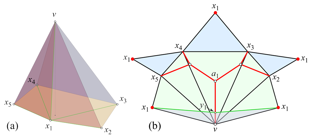
Figure 4.3: (a) A pyramid with pentagonal base $X$. Shortest paths from $x_{1}$ to all vertices are marked green. (b) The star-unfolding with respect to $x_{1}$. The triangles from $X$ are blue; those from $L$ are green. $C(x_{1})\subset L$ is red. The digon $D_{1}=(x_{1},y_{1})$ is shaded.

The digon $D_{1}(x_{1},y_{1})$ surrounding $v$ places $y_{1}$ on the $va_{1}$ segment of $C(x_{1},P)=C(x_{1})$. If one imagines $y_{1}$ sliding along $va_{1}$ from $v$ to $a_{1}$, the digon angle at $x_{1}$, call it ${\delta}_{1}$, increases. To show that $y_{1}$ can be placed so that ${\delta}_{1}$ is large enough to reduce the angle at $x_{1}$ to its angle in $X$ will require $a_{1}$ to lie in $L$ (rather than in $X$).

It turns out that $C(x_{1})\subset L$ follows from a lemma in [AAOS97]. However, after removing $D_{1}$ and invoking Alexandrov’s Gluing Theorem, we can no longer apply this lemma. With this background, we now proceed to the general case.

Claim (1): $C(x_{i+1},P_{i})\subset L$.

Assume we have removed digons at $x_{1},\ldots,x_{i}$, so that $P_{i}=X_{i}\cup L_{i}$, and $L_{i}$ contains one vertex $y_{i}$, the endpoint of the last digon $D_{i}$ removed, and $X_{i}$ contains no vertices. Assume to the contrary of Claim (1) that $C(x_{i+1},P_{i})=C(x_{i+1})$ includes a point $z$ strictly interior to $X_{i}$. Because $z\in C(x_{i+1})$, there are two geodesic segments from $x_{i+1}$ to $z$, call them ${\gamma}^{z}_{1}$ and ${\gamma}^{z}_{2}$. Because $X_{i}$ contains no vertices, it cannot be that both ${\gamma}^{z}_{1}$ and ${\gamma}^{z}_{2}$ are in $X_{i}$. Say that ${\gamma}^{z}_{1}$ crosses $L_{i}$. Let $p\in\partial X$ be the first point at which ${\gamma}^{z}_{1}$ enters $X_{i}$, and let ${\gamma}_{1}\subset{\gamma}^{z}_{1}$ be the portion from $x_{i+1}$ to $p$. See Fig. 4.4.

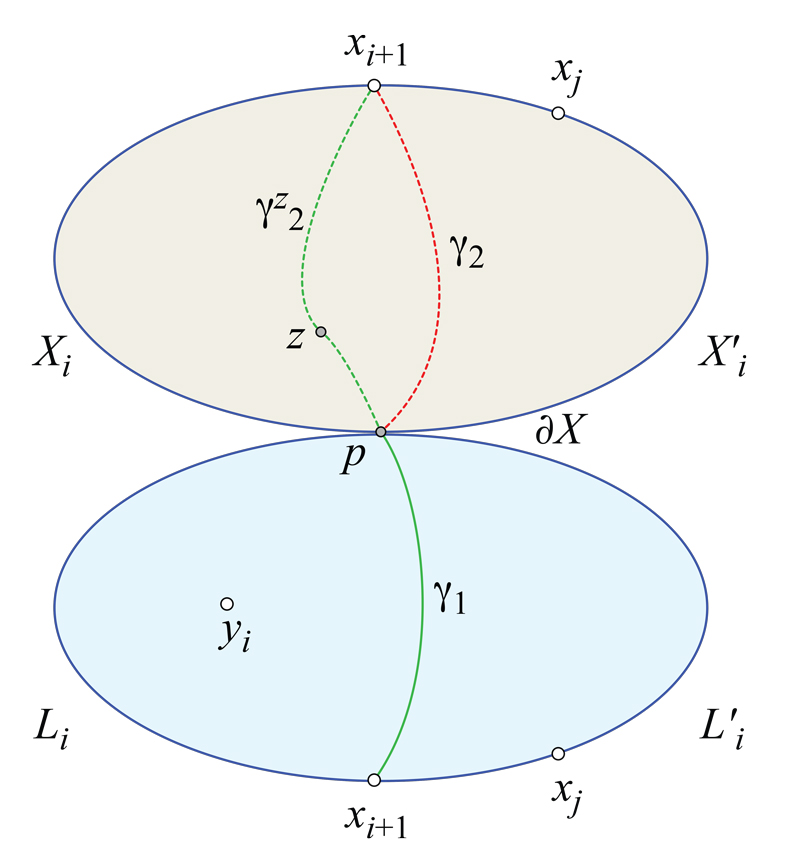
Figure 4.4: $X_{i}$ is flipped above $L_{i}$ in this abstract illustration. Cauchy’s Arm Lemma ultimately shows that $\ell({\gamma}_{1})\geq\ell({\gamma}_{2})$.

The geodesic segment ${\gamma}_{1}$ divides $L_{i}$ into two parts; let $L^{\prime}_{i}$ be the part that does not contain the vertex $y_{i}$. Join $x_{i+1}$ to $p$ with a geodesic ${\gamma}_{2}$ lying in $X_{i}$. ${\gamma}_{2}$ was a shortest path to $p$ in $X$, but may no longer be shortest in $X_{i}$. ${\gamma}_{2}$ also divides $X_{i}$ into two parts; let $X^{\prime}_{i}$ be the part sharing a portion of $\partial X$ with $L^{\prime}_{i}$.

Now we will argue that $\ell({\gamma}_{1})\geq\ell({\gamma}_{2})$, where $\ell({\gamma})$ is the length of ${\gamma}$. This will yield a contradiction, for the following reasons. ${\gamma}_{1}$ is a shortest geodesic to $p$, because it extends to ${\gamma}^{z}_{1}$, which is a shortest geodesic to $z$. So ${\gamma}_{2}$ cannot be strictly shorter than ${\gamma}_{1}$. Therefore we must have $\ell({\gamma}_{1})=\ell({\gamma}_{2})$, which implies that $p\in C(x_{i+1})$. But then ${\gamma}_{1}$ cannot continue to ${\gamma}^{z}_{1}$ beyond $p$, as $p$ is a cut point.

To reach $\ell({\gamma}_{1})\geq\ell({\gamma}_{2})$, we will use the extension of Cauchy’s Arm Lemma described in Chapter 2. Let ${\theta}^{X}_{j}$ be the angle at $x_{j}$ in $X_{i}$, and ${\theta}^{L}_{j}$ be the angle at $x_{j}$ in $L_{i}$. For $j>i+1$, we know that ${\theta}^{L}_{j}>{\theta}^{X}_{j}$ because $P$ is a pyramid (see Lemma 2.8) and digon removal has not yet reached $x_{j}$. We also know that ${\theta}^{X}_{j}\leq\pi$ because $X$ is convex. However, ${\theta}^{L}_{j}$ could be nearly as large as $2\pi-{\theta}^{X}_{j}$ if the pyramid $P$’s apex $v$ projects outside the base $X$.

Let $c_{X}$ be the planar convex chain in $\partial X$ that corresponds to $X^{\prime}_{i}$; assume $c_{X}$ is $x_{i+1},x_{i+2},\ldots,x_{j},\ldots,p$ with angles ${\theta}^{X}_{j}$. (The case where $c_{X}$ is includes the other part of $\partial X$, $x_{i+1},x_{i},\ldots,p$ can be treated analoguously.) Then $\ell({\gamma}_{2})$ is the length of the chord between $c_{X}$’s endpoints. In order to apply Cauchy’s lemma, we rephrase the angles at $x_{j}$ as turn angles ${\tau}_{j}=\pi-{\theta}^{X}_{j}$. The extension of Cauchy’s lemma guarantees that, if the chain angles are modified so that the turn angles lie within $[-{\tau}_{j},{\tau}_{j}]$, then the endpoints chord length cannot decrease. Roughly, opening (straightening) the angles stretches the chord.

Define $c_{L}$ as the planar (possibly nonconvex) chain composed of the same vertices $x_{j}$ that define $c_{X}$, but with angles ${\theta}^{L}_{j}$. Because ${\theta}^{L}_{j}\leq 2\pi-{\theta}^{X}_{j}$, the turn angles $\pi-{\theta}^{L}_{j}$ in $c_{L}$ satisfy

$$\pi-{\theta}^{L}_{j}\geq\pi-(2\pi-{\theta}^{X}_{j})=-(\pi-{\theta}^{X}_{j})=-{\tau}_{j}\;.$$

Also, because ${\theta}^{L}_{j}>{\theta}^{X}_{j}$,

$$\pi-{\theta}^{L}_{j}\leq\pi-{\theta}^{X}_{j}={\tau}_{j}\;.$$

So the $c_{L}$ turn angles are in $[-{\tau}_{j},{\tau}_{j}]$, and we can conclude from Theorem 2.7 that the $c_{L}$ endpoints chord length $\ell({\gamma}_{1})$ is at least $\ell({\gamma}_{2})$, the $c_{X}$ endpoints chord length.

We have now reached $\ell({\gamma}_{1})\geq\ell({\gamma}_{2})$, whose contradiction described earlier shows that indeed $C(x_{i+1})\subset L_{i}$.

Claim (2): ${\alpha}_{i+1}\geq{\theta}^{L}_{i+1}-{\theta}^{X}_{i+1}$.

Recall that ${\alpha}_{i+1}$ is the angle at $x_{i+1}$ of the digon from $x_{i+1}$ to $a_{i+1}$, the first ramification point of $C(x_{i+1})$ beyond the vertex $y_{i}$. The claim is that ${\alpha}_{i+1}$ is large enough to reduce ${\theta}^{L}_{i+1}$ to ${\theta}^{X}_{i+1}$. We establish this by removing a path from $C(x_{i+1})$ and tracking angles, as follows.

From Claim (1), $C(x_{i+1})\subset L_{i}$. Let ${\rho}_{i,i+2}$ be the path in the tree $C(x_{i+1})$ from $x_{i}$ to $x_{i+2}$. See Fig. 4.5.

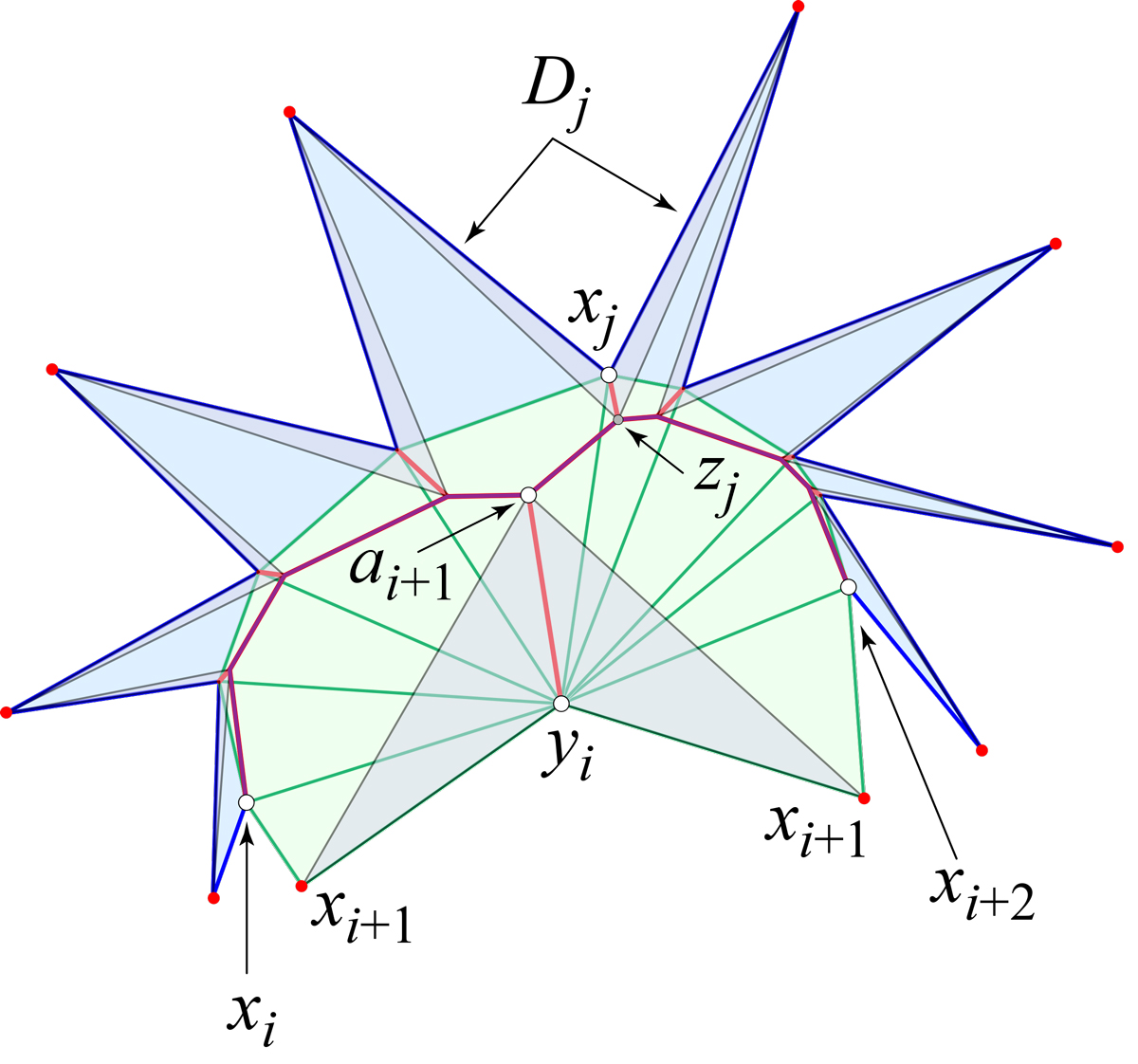
Figure 4.5: Star-unfolding of a pyramid with respect to $x_{i+1}$. The triangles from $X_{i}$ are blue; those from $L_{i}$ are green. Red points are images of $x_{i+1}$. Digons are shaded. ${\rho}_{i,i+2}$ is purple; remainder of $C(x_{i+1})$ is red.

Removal of ${\rho}_{i,i+2}$ from $C(x_{i+1})$ disconnects $C(x_{i+1})$ into the edge $y_{i}a_{i+1}$, and a series of subtrees $T_{j}$. Each $T_{j}$ shares a point $z_{j}$ with $C(x_{i+1})$. Let $D_{j}$ be the digon from $x_{i+1}$ to $z_{j}$, and let ${\delta}_{j}$ be the angle of $D_{j}$ at $x_{i+1}$. Finally, let ${\Delta}_{j}=\sum_{j}{\delta}_{j}$.

Note that all the ${\delta}_{j}$ angles are in $X_{i}$. In contrast, the angle at $x_{i+1}$ in the digon $D_{i+1}=D(x_{i+1},a_{i+1})$ is in $L_{i}$, as illustrated in Fig. 4.5. We defer justifying this claim to later.

Cut off all $D_{j}$, and also cut off $D_{i+1}$. Suture the surface closed; call it $P^{*}=X^{*}\cup L^{*}$. By Lemma 2.6, the cut locus $C(x_{i+1},P^{*})$ is precisely the path ${\rho}_{i,i+2}$. Therefore, by Lemma 2.2, $P^{*}$ is a doubly-covered convex polygon, so all angles at $x_{j}$ are equal above in $L^{*}$ and below in $X^{*}$. In particular, ${\theta}^{X^{*}}_{i+1}={\theta}^{L^{*}}_{i+1}$. Now, because ${\Delta}$ angle was removed from ${\theta}^{X}_{i+1}$, ${\theta}^{X^{*}}_{i+1}={\theta}^{X}_{i+1}-{\Delta}$. Because ${\alpha}_{i+1}$ was removed from ${\theta}^{L}_{i+1}$, ${\theta}^{L^{*}}_{i+1}={\theta}^{L}_{i+1}-{\alpha}_{i+1}$. Therefore,

$${\theta}^{L}_{i+1}-{\alpha}_{i+1} = {\theta}^{X}_{i+1}-{\Delta}\;\leq\;{\theta}^{X}_{i+1}$$ (4.1)

$${\alpha}_{i+1} \geq {\theta}^{L}_{i+1}-{\theta}^{X}_{i+1}$$ (4.2)

which is Claim (2).

It remains to show that $D_{i+1}$ is in $L_{i}$ rather than in $X_{i}$. Suppose to the contrary that all the angle removal was in $X_{i}$. Then ${\theta}^{L}_{i+1}={\theta}^{X}_{i+1}-{\Delta}-{\alpha}_{i+1}$. So ${\theta}^{L}_{i+1}<{\theta}^{X}_{i+1}$, which is not possible for $P$ a pyramid. This completes the proof of Claim (2) and the lemma. ∎

4.3.2 General case

Lemma 4.3 is special in that $P$ sits over a base $X$. In the general situation, $X$ is the intersection of $Q$ with the truncating slice plane $\Pi$, but $X$ is not a face of $Q$. Rather in general, $X$ is inside $Q$, the “top” of the portion $Q^{\prime}$ of $Q$ below $\Pi$.

Lemma 4.4.

Let $Q$ be obtained from $P$ by truncating vertex $v$. Then, if $v$ has degree-$k$, $Q$ may be obtained from $P$ by $k-1$ tailoring steps, each the excision of a digon surrounding one vertex.

Proof.

Here we argue that the general case is in some sense no different than the special case of $P$ a pyramid just established in Lemma 4.3. In fact, the exact same digon excisions suffice to tailor $P$ to $Q$.

First we establish additional notation. Let $\Pi$ be the plane slicing off $v$ above $\Pi$, and let $X=\Pi\cap P$. Let the “bottom” part of $P$ be $Q^{\prime}$, with the final polyhedron $Q=Q^{\prime}\cup X$. We continue to use $L$ to denote the portion of $P$ above $\Pi$, so $P=Q^{\prime}\cup L$. After removal of digons at $x_{1},x_{2},\ldots,x_{i}$, we have $P_{i}=Q^{\prime}_{i}\cup L_{i}$.

Below it will be important to distinguish between the three-dimensional extrinsic shape of $Q^{\prime}_{i}$ and its intrinsic structure determined by the gluings that satisfy Alexandrov’s Gluing Theorem. We will use $\bar{Q}^{\prime}_{i}$ for the embedding in ${\mathbb{R}}^{3}$ and $Q^{\prime}_{i}$ for the intrinsic surface, and we will similarly distinguish between $\bar{X}_{i}$ and $X_{i}$. Note that we can no longer assume that $C(x_{i+1},P_{i})\subset L_{i}$, for the cut locus could extend into $Q^{\prime}$ (whereas it could not extend into $X$ in Lemma 4.3).

It suffices to show by induction that, on $P_{i}$, the following statements hold:
(a) The shortest path ${\gamma}_{i+1}$ joining $x_{i+1}$ to $y_{i}$ is included in $L_{i}$.
(b) The ramification point $a_{i+1}$ is still on $L_{i}$.
(c) The $x_{i+1}$ angle ${\alpha}_{i+1}$ of the digon $D_{i+1}=D(x_{i+1},a_{i+1})$ is larger than or equal to ${\omega}_{Q}(x_{i+1})-{\omega}_{P}(x_{i+1})$ (and so sufficient to reduce the curvature to ${\omega}_{Q}(x_{i+1})$).

To see (a), assume, on the contrary, that ${\gamma}_{i+1}$ intersects $Q^{\prime}_{i}$. Assume, for the simplicity of the exposition, that ${\gamma}_{i+1}$ enters $Q^{\prime}_{i}$ only once, at $x_{i+1}$, and exits $Q^{\prime}_{i}$ at $p\in\partial X$. Let ${\gamma}^{\prime}_{i+1}$ denote the part of ${\gamma}_{i+1}$ between $x_{i+1}$ and $p$.

We now check (a) for $i=0$. $Q=Q^{\prime}\cup X$ and $X$ is planar, hence, because the orthogonal projection of any rectifiable curve onto a plane shortens or leaves its length the same, ${\gamma}^{\prime}_{1}$ is longer than or has the same length as its projection ${\gamma}^{\prime\prime}_{1}$ onto $X$. So $p$ is a cut point of $x_{1}$ along ${\gamma}_{1}$, contradicting the extension of ${\gamma}_{1}$ as a geodesic segment beyond $p$.

By the induction assumption, all the digon excisions occur on $L_{i}$; $Q^{\prime}_{i}$ is unchanged. Nevertheless, as part of $P_{i}$, neither $\bar{Q}^{\prime}_{i}$ nor $\bar{X}_{i}$ is (in general) congruent to the original $\bar{Q}$ and $\bar{X}$. However, if we consider $Q^{\prime}_{i}$ and $X_{i}$ separate from $P_{i}$, we can reshape them so that $\bar{Q}^{\prime}_{i}=\bar{Q}$ and $\bar{X}_{i}=\bar{X}$, precisely because they have not changed. Then $\bar{X}$ is planar and the projection argument used for $i=0$ works for all $i$.

Next we check (b) and (c) for $i=0$. Consider, as in Lemma 4.3, the digon $D_{1}=(x_{1},y_{1})$ with $y_{1}\in C(x_{1})$, with again $a_{1}$ the first ramification point of $C(x_{1})$ beyond $v$. The direction at $v$ of the edge $va_{1}$ is only determined by the geodesic segment from $x_{1}$ to $v$, and hence is not influenced at all by $Q^{\prime}$, because, by $i=0$ in (a), that segment lies in $L$.

The ramification point $a_{1}$ is joined to $x_{1}$ by three geodesic segments, two of them—say ${\gamma}_{1}$ and ${\gamma}_{2}$—included in $L$. The third geodesic ${\gamma}_{3}$ starts from $x_{1}$ towards $Q^{\prime}$ and finally enters $L$ to connect to $a_{1}$. See Fig. 4.6. Because these three geodesics have the same length, the longer ${\gamma}_{3}$ is, the longer are ${\gamma}_{1}$ and ${\gamma}_{2}$, and therefore more distant is $a_{1}$ to $v$. So $a_{1}$ is closest to $v$, and the segment $va_{1}$ shortest, when $Q^{\prime}=X$ and $P$ is a pyramid. It is when $va_{1}$ is shortest that there is the least “room” for $y_{1}$ on $va_{1}$ to achieve the needed digon angle at $x_{1}$, for that angle is largest when $y_{1}$ approaches $a_{1}$. Therefore, the case when $Q^{\prime}=X$ and $P$ is a pyramid is the worst case, already settled in Lemma 4.3.

Figure 4.6: Three geodesics to ramification point $a_{1}$ on $C(x_{1})$. Dashed ${\gamma}_{3}$ partially in $Q^{\prime}$. The same situation holds under the changes: $x_{1}\to x_{i+1}$, $a_{1}\to a_{i+1}$, $v\to y_{i}$, $Q^{\prime}\to Q^{\prime}_{i}$, $L\to L_{i}$.

Now we treat the general case for (b) and (c). Again by the induction assumption, all changes to $P_{i}$ were made on its “upper part” $L_{i}$.

Because we ultimately need to reduce $L$ to $X$, the angle ${\omega}_{Q}(x_{i+1})-{\omega}_{P}(x_{i+1})$ necessary to be excised at $x_{i+1}$, does not depend on $Q^{\prime}_{i}$, only on $L_{i}$. Thus the argument used for $i=0$ carries through. The situation depicted in Fig. 4.6 remains the same, with $x_{1}$ replaced by $x_{i+1}$, $v$ replaced by $y_{i}$, and $a_{1}$ replaced by $a_{i+1}$. The ramification point $a_{i+1}$ is closest to $y_{i}$, and the segment $y_{i}a_{i+1}$ shortest, when $Q^{\prime}=X$ and $P$ is a pyramid. It is when $y_{i}a_{i+1}$ is shortest that there is the least “room” for $y_{i+1}$ on $y_{i}a_{i+1}$ to achieve the needed angle excision at $x_{i+1}$, for that angle is largest when $y_{i+1}$ approaches $a_{i+1}$. Therefore, the case when $Q^{\prime}=X$ and $P$ is a pyramid is the worst case, already settled in Lemma 4.3. ∎

Note that, in the end, the digon removals in Lemma 4.2, and then in Lemma 4.3, also work in the general case, Lemma 4.4.

4.4 Cube/Tetrahedron: Completion

4.4.1 Pyramid Removals

We now return to the cube/tetrahedron example started in Chapter 3. We had reduced the sliced-off portion of the original cube $P$ to four pyramids $P_{1},P_{2},P_{3},P_{4}$. Now each of these pyramids needs to be “tailored away” to leave the goal tetrahedron $Q$. Fig. 4.7 shows that when processed in order, their removal reduces the portion of $P$ “above” $Q$, leaving the goal tetrahedron $Q$.

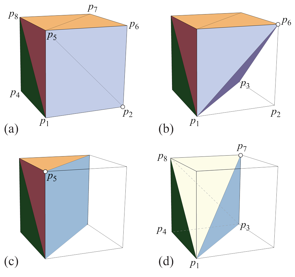
Figure 4.7: Pyramid removals. The apex of the pyramid to be next removed is highlighted. From (a) to (b), the pyramid $P_{1}$ with apex $p_{2}$ and base $p_{1}p_{3}p_{6}$ is removed. Then $P_{2}$ apexed at $p_{6}$ is removed, producing (c), then removing $P_{3}$ apexed at $p_{5}$ leads to (d). The final removal of $P_{4}$ apexed at $p_{7}$, leaves the tetrahedron $Q=p_{1}p_{3}p_{4}p_{8}$ previously illustrated in Fig. 3.2(a).

4.4.2 Pyramid Reductions by Tailoring

Now we follow Lemma 4.4 to reduce each of the four pyramids to their bases. We only illustrate this for the first pyramid removed, $P_{1}$, with apex $p_{2}$ and base $X=p_{1}p_{3}p_{6}$. See Fig. 4.8(a). The base is an equilateral triangle, with edge lengths $\sqrt{2}$, with the apex is connected to the base vertices by unit-length edges. Because the apex $p_{2}$ is a cube corner, it has three incident $90^{\circ}$ angles, so ${\omega}(p_{2})=90^{\circ}$. The three faces incident to $p_{2}$ are $45^{\circ}{-}45^{\circ}{-}90^{\circ}$ triangles. The base angles in $X$ are $60^{\circ}$. So each digon must reduce the incident $90^{\circ}$ angles by $30^{\circ}$ to match $60^{\circ}$. Starting with $p_{1}$, the digon geodesics are $\pm 15^{\circ}$ around the $p_{1}p_{2}$ edge.

The geometry is clearest if we unfold $P_{1}$’s lateral faces into the plane, as shown Fig. 4.8(b). Excising the first digon and sealing the cut results in a new polyhedron, with the apex $p_{2}$ replaced by a new vertex, call it $y$, of curvature ${\omega}(y)=60^{\circ}$ (because the two digon angles must sum to the $90^{\circ}$ curvature at $p_{2}$). Unfortunately, we cannot display this new polyhedron because of the difficulty of constructing what AGT guarantees exists.

Lemma 4.4 says that just one more digon needs removal (because $p_{2}$ has degree $k=3$), again $\pm 15^{\circ}$ this time around the $p_{3}y$ edge. This removal reduces $P_{1}$ to its equilateral triangle base, and, despite the nonconstructive nature of AGT, we know that the full polyhedron is exactly what we illustrated earlier in Fig. 4.7(b).

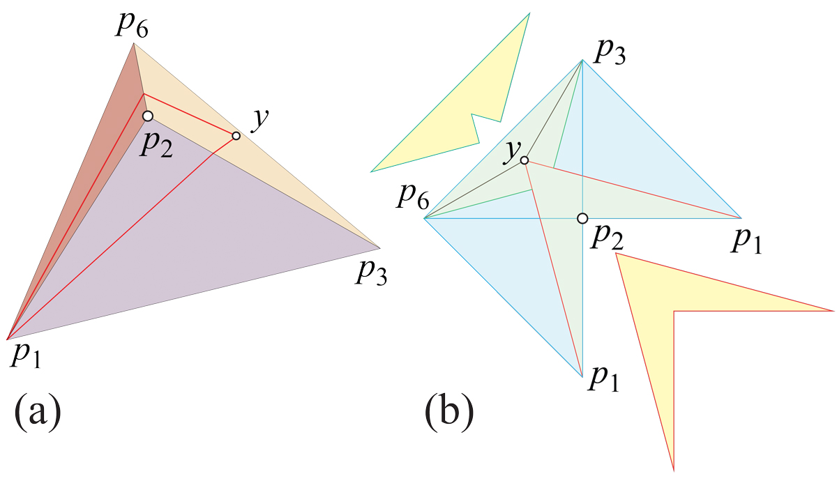
Figure 4.8: (a) Pyramid $P_{1}$: apex $p_{2}$, base $p_{1}p_{3}p_{6}$. (b) Excision of two digons. Each is bound by geodesics $\pm 15^{\circ}$ about the edge to $p_{2}$. After removing $p_{2}$, a new vertex $y$ is created. The removal of $y$ in the second excision flattens the pyramid to its base.

One further remark on the shape of $P_{1}$ after excision of the first digon. If we imagine $P_{1}$ standing alone on its base $X$ as illustrated in Fig. 4.8(a), rather than as part of the full cube polyhedron, then it is not difficult to reconstruct the shape of $P^{\prime}_{1}$. It is a flat doubly-covered quadrilateral, with the triangle $p_{3}yp_{6}$ flipped over and joined to the $p_{3}p_{6}$ edge of the equilateral triangle base $X$. However, with this $P^{\prime}_{1}$ piece joined to the full cube, it seems much less straightforward to determine the shape of the full polyhedron.

Each pyramid reduction proceeds in the same manner: $k-1$ digons are excised if the apex has degree-$k$, and the lateral faces are reduced to the base. So $P_{2}$ has apex $p_{6}$ and base $p_{1}p_{3}p_{5}p_{7}$. After removal of three digons, the result is as illustrated in Fig. 4.7(c). $P_{3}$’s apex $p_{5}$ has degree-$3$, so two digon removals lead to (d). The last pyramid removed, $P_{4}$, reduces to the face $p_{1}p_{3}p_{8}$ of $Q$, completing the tailoring of the cube $P$ to tetrahedron $Q$.

4.4.3 Seals

After removal of the two digons illustrated in Fig. 4.8(b), $P_{1}$ has been reduced to its equilateral triangle base $X$. Sealing the first digon produces a seal ${\sigma}_{1}$, which is then clipped to a segment $s_{1}$ by the second digon removal, which produces ${\sigma}_{2}$ along the boundary of $X$. The seal segments then are as shown in Fig. 4.9(a).

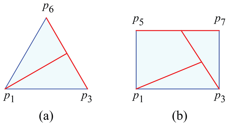
Figure 4.9: (a) Base of $P_{1}$. (b) Base of $P_{2}$. Seal segments: red.

Fig. 4.9(b) shows the three seal segments that result by reducing $P_{2}$ to its base. These depictions of the seal graph ${\Sigma}$ will be explored in some detail in Chapter 5.

There is an aspect of the seals we are not tracking: As can be seen in Fig. 4.7(b,c), one of the faces of $P_{2}$ is the equilateral triangle base of $P_{1}$. Since that base is already crossed by seal segment $s_{1}$ when $P_{2}$ is undergoing digon removal, that segment $s_{1}$ will be reflected as a cut in the reduced base of $P_{2}$, not depicted in Fig. 4.9(b). We have not attempted to track this complex overlaying of seal cuts in the surface of $P$. However, we explore seals for one pyramid tailoring in some detail in Chapter 5.

4.5 Hexagonal Pyramid Example

We now detail a more complex example following Lemma 4.3 to tailor a pyramid $P$ to its base $X$. We continue to employ the notation used in the lemmas above. The example is shown in Fig. 4.10. $X$ is a regular hexagon, and $L$ consists of $k=6$ congruent, $70^{\circ}{-}70^{\circ}{-}40^{\circ}$ isosceles triangles. The curvature at the apex $v$ is $360^{\circ}-6\cdot 40=120^{\circ}$. The angle at each $x_{i}$ in $X$ is $120^{\circ}$ whereas the angle in $L$ is $140^{\circ}$. So each digon excision must remove $20^{\circ}$ from $x_{i}$. As in the lemmas, we excise the digons in circular order around $\partial X$.

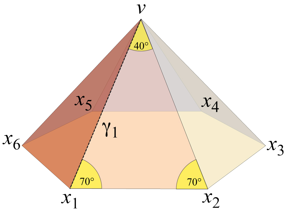
Figure 4.10: Pyramid with regular hexagon base $X$; all lateral faces congruent triangles.

We display the progress of the excisions on the layout of $L$ in Fig. 4.11(a). Let $v=y_{0}$ for ease of notation. $D_{1}=(x_{1},y_{1})$ includes the geodesic ${\gamma}_{1}$ from $x_{1}$ to $y_{0}$, and locates $y_{1}$ on the cut locus segment as described in the lemmas. The digon boundary geodesics each remove $10^{\circ}$ from the left and right neighborhood of $x_{1}$, and meet at $y_{1}$ at an angle of $100^{\circ}$, which is then the curvature at the new vertex: ${\omega}(y_{1})=100^{\circ}$. Notice that the digon angles $20^{\circ}+100^{\circ}$ match the curvature ${\omega}(v)=120^{\circ}$ removed, as they must to satisfy Gauss-Bonnet.

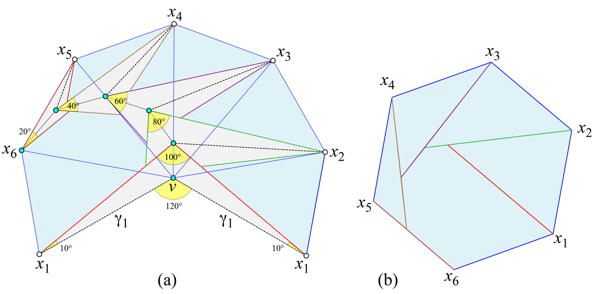
Figure 4.11: (a) Cone $L$ flattened; ${\omega}(v)=120^{\circ}$. Digons $D_{i}=(x_{i},y_{i-1})$ shaded. Dashed lines are geodesics ${\gamma}_{i}$ from $x_{i}$ to the vertex $y_{i-1}$ (with $y_{0}=v$). (b) After excising all digons $D_{1},\ldots,D_{5}$, $L_{5}$ is isometric to $X$. Seals $\tilde{{\sigma}}_{i}$ are marked.

One should imagine that $D_{1}$ is sutured closed in Fig. 4.11(a), producing $L_{1}$, before constructing $D_{2}(x_{2},y_{2})$. Let ${\sigma}_{i}$ be the geodesic on $L_{i}$ that results from sealing $D_{i}$ closed; ${\sigma}_{i}$ is like a “scar” from the excision. Notice that one of the geodesics bounding $D_{2}$ crosses ${\sigma}_{1}$.

This pattern continues as all $k{-}1=5$ digons are removed, each time replacing vertex $y_{i-1}$ with $y_{i}$, flattening the curvature ${\omega}(y_{i})={\omega}(y_{i-1})-20^{\circ}$. Finally, after $D_{5}(x_{5},y_{5})$ is removed, $y_{5}$ is coincident with $x_{6}$. No further digon removal is needed, because $D_{5}$ removed $20^{\circ}$ from $x_{6}$. So now each angle in $L_{k}=L_{5}$ at all $k{=}6$ vertices is $120^{\circ}$, and $L_{5}$ is isometric to a flat regular hexagon, i.e., to $X$.

This final hexagon is shown in Fig. 4.11(b). The images $\tilde{{\sigma}}_{i}$ of the seals are in general clipped versions of ${\sigma}_{i}$ on $L_{i}$, clipped by subsequent digon removals. The particular circular order of digon removal followed in this example and the lemmas result in a spiral pattern formed by $\tilde{{\sigma}}_{i}$. Other excision orderings, which ultimately would result in the same flat $L_{k-1}$ (effectively proved in Lemmas 4.2–4.4) would create different seal patterns. As mentioned earlier, we study seals in detail in Chapter 5.

4.6 Tailoring is finer than sculpting

In this section we reach one of our main results, Theorem 4.6, which says, roughly, that any polyhedron $Q$ that can be obtained by sculpting $P$ can be obtained by tailoring $P$. Moreover, Lemma 4.5 shows that polyhedra can be obtained by tailoring that cannot be obtained by sculpting. So, in a sense, tailoring is finer than sculpting.

Lemma 4.5.

There are shapes $P$ and sequences of tailorings of $P$ that result in polyhedra not achievable by sculpting.

Proof.

We first tailor a regular tetrahedron $T$ as in Example 1.1, resulting in the kite $K$ in Fig. 1.2(b). We now show that $K$ cannot fit inside $T$, so it couldn’t have been sculpted from $T$. Assume $T$ has edge-length $1$. Then its extrinsic diameter is $1$ and its intrinsic diameter is $2/\sqrt{3}$ (see, e.g., Theorem 3.1 in [Rou03]). Moreover, the extrinsic diameter of $K$ is precisely the intrinsic diameter of $T$, and so it cannot fit inside $T$.

Next we construct a non-degenerate example, a modification of the previous one. Consider a non-degenerate pentahedron $F$ close enough to $K=oac_{d}b$ in Fig. 1.2(b). For example, it could have two vertices close to the vertex $a$ of $K$. Insert into $F$ the removed digon from $T$; this is not affected by the new vertex, because it does not interfere with the geodesic segment from $c_{d}$ to $o$. We arrive at some surface $P$ close enough to the original tetrahedron $T$. Therefore, the intrinsic and extrinsic diameters of $P$ and $F$ are close enough to those of $K$ and $T$, respectively, and the above inequality between the extrinsic diameters of $P$ and $F$ still holds, because of the “close enough” assumption. ∎

Theorem 4.6.

Let $P$ be a convex polyhedron, and $Q\subset P$ a convex polyhedron resulting from repeated slicing of $P$ with planes. Then $Q$ can also be obtained from $P$ by tailoring. Consequently, for any given convex polyhedra $P$ and $Q$, one can tailor $P$ “via sculpting” to obtain any homothetic copy of $Q$ inside $P$.

Proof.

Lemma 4.1 established that one slice leads to domes, Theorem 3.2 showed that each dome leads to pyramids, and Lemma 4.4 showed that each pyramid can be reduced to its base by tailoring. Since this holds for one slice, it immediately follows that it holds for arbitrary slicing.

Concerning the domes $\to$ pyramids step, we note that the property that each pyramid $P_{i}$ has a common edge with $X$, established in Theorem 3.2, allows reduction of the pyramids in the order that they are obtained in that theorem. After each reduction, the result is still a g-dome, allowing iteration until the original g-dome is reduced to its base.

For the homothet-copy claim of the lemma, shrink $Q$ by a dilation until it fits inside $P$, and then apply the reductions. ∎

As we mentioned in the Preface, an informal consequence of this theorem is that $P$ can be “whittled” to e.g., a sphere $S$:

Corollary 4.7.

For any convex polyhedron $P$ and any convex surface $S$, one can tailor $P$ to approximate a homothetic copy of $S$.

Proof.

Bring a homothetic copy of $S$ inside $P$. Perform a series of slicings of $P$ with planes tangent to $S$. Any degree of approximation desired can be achieved by increasing the number of plane splicings. Call the result of these slicings $Q$. Now apply Theorem 4.6. ∎

Despite this corollary, it does not seem possible to accomplish the reverse: to start with a strictly convex surface and tailor it to a polyhedron. However, one can of course sculpt a surface to a polyhedron.

Chapter 5 Pyramid Seal Graph

5.1 Pyramid Digon Removal

As we have seen in Theorem 4.6, tailoring by tracking sculpting ultimately relies on digon removal reducing pyramids to their bases. We have illustrated such reductions for a few low-degree pyramids in Figs. 4.2, 4.8, and 4.11. In the latter two figures, we displayed the seals $\tilde{{\sigma}_{i}}$ on the base $X$ after reduction. It however remains difficult to grasp in detail the digon-removal process for a pyramid $P$, for at least three reasons:

1. After removing the first digon $D_{1}$, $P_{1}$ is (in general) no longer a pyramid. The difficulty of computationally realizing the subsequent intermediate shapes $P_{i}$, guaranteed by AGT, makes it hard to envision the process.

2. The seals ${\sigma}_{i}$ that result from closing digon $D_{i}$ cross and clip one another.

3. The process depends on the order in which the digons are removed.

We will continue to circumvent this last difficulty by only studying the natural order of digon removal, anchored at $x_{1},x_{2},x_{3},\ldots$ in counterclockwise order around $\partial X$. In this section, we introduce a different way to view digon removal that in some sense skirts the first two difficulties.

The process is complex enough to require somewhat extensive notation, which we list in two parts before turning to examples.

5.1.1 Notation I

• $P$: a pyramid, $n$ vertices around base $X$.

• Base vertices $x_{1},x_{2},\ldots,x_{n}$, in counterclockwise order around $\partial{X}$.

• Apex $y_{0}$ of degree-$n$.

• $y_{i}$: apex after removing digon $D_{i}$.

• $D_{i}$: digon from $x_{i}$ to $y_{i}$, surrounding $y_{i-1}$.

• $L_{i}$: (the remaining of the) lateral faces after removing digon $D_{i}$. $L_{0}$: initial faces before any removals. The apex of $L_{i}$ is $y_{i}$.

• $P_{i}$: The polyhedron $L_{i}\cup X$, guaranteed by AGT. $P=P_{0}$ is the original, before any digon removal.

We should emphasize that although $P_{i}=L_{i}\cup X$, in general $X$ will not be planar in $P_{i}$ as it is in $P_{0}$, and so $P_{i}$ is not a pyramid, as previously mentioned.

5.2 Cone Viewpoint

Although we do not know the structure of $P_{i}$, except at the beginning ($i=0$) and end ($i=n{-}1$), when it is $P$ and doubly-covered $X$ respectively, we do know that the lateral faces $L_{i}$ contain only one vertex, $y_{i}$, hence they form a subset of a cone apexed at $y_{i}$. Any cone can be cut open along a generator (a ray on the cone from the apex) and laid flat in the plane. Such a layout will have an angle gap of ${\omega}(y_{i})$ at the apex. It is especially useful to cut along $x_{i}y_{i-1}$ before removing digon $D_{i}$. We will provide several examples, after presenting more notation. We emphasize the indices $i{-1}$, $i$, and $i{+}1$ in the following, in an attempt to avoid confusion.

5.2.1 Notation II

• $\bar{L}_{i-1}$: Unfolding of $L_{i-1}$ cut open along $x_{i}y_{i-1}$. So after removing and sealing digon $D_{i-1}$, but not yet $D_{i}$.

• $\bar{L}_{i}$: Unfolding of $L_{i}$ cut open along $x_{i+1}y_{i}$. So after removing and sealing digon $D_{i}$, but not yet $D_{i+1}$. So $\bar{L}_{0}$ is $L_{0}$ cut open along $x_{1}y_{0}$, and $\bar{L}_{1}$ is $L_{1}$ cut open along $x_{2}y_{1}$.

• ${\sigma}_{i}=x_{i}y_{i}$ is the $i$-th seal after suturing closed the digon $D_{i}$. We view the seals as directed from $x_{i}$ to $y_{i}$, so that they have distinguished left and right sides. This direction is only used in the proofs; the seals are illustrated as undirected segments in several figures. When the direction plays a role, we use boldface: $\bm{{\sigma}}_{i}$.

• ${\Sigma}_{i}$: the seal graph after removing digon $D_{i}$. ${\Sigma}_{0}=\varnothing$, and ${\Sigma}_{1}=x_{1}y_{1}$.

• $s_{j}\subseteq{\sigma}_{j}$, $1\leq j\leq i$, is the possibly truncated seal segment in ${\Sigma}_{i}$, on the surface $P_{j}$. So, after possibly other truncations, we reach $\tilde{{\sigma}_{j}}$, hence the informal inclusion $\tilde{{\sigma}_{i}}\subseteq s_{j}\subseteq{\sigma}_{j}$; “informal” because those geodesic segments live in different spaces.

• $S_{i}$ is the subset of $L_{i}$ bounded by $x_{1}y_{i}$ and $x_{i}y_{i}$, the sealed region which we will later prove contains ${\Sigma}_{i}$.

5.3 Examples

We start with $P_{1}$, previously displayed in Fig. 4.8. $X$ is an equilateral triangle, with the apex centered above its centroid. Fig. 5.1 shows the removal of $n{-}1=2$ digons $D_{1},D_{2}$ that reduce $L_{0}$ to the equilateral triangle base $X$. Images are repeated so that in one row the transition from $L_{i-1}$ to $L_{i}$ by removal of $D_{i}$ is evident.

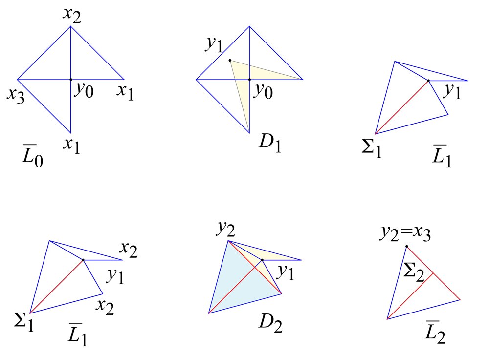
Figure 5.1: $P_{1}$. $X$ is an equilateral triangle. Cf. Fig. 4.9(a).

Next is the more complicated $P_{2}$ in Fig. 5.2. Here $X$ is a rectangle, and three digons are removed, $D_{1},D_{2},D_{3}$, before reaching $X$.

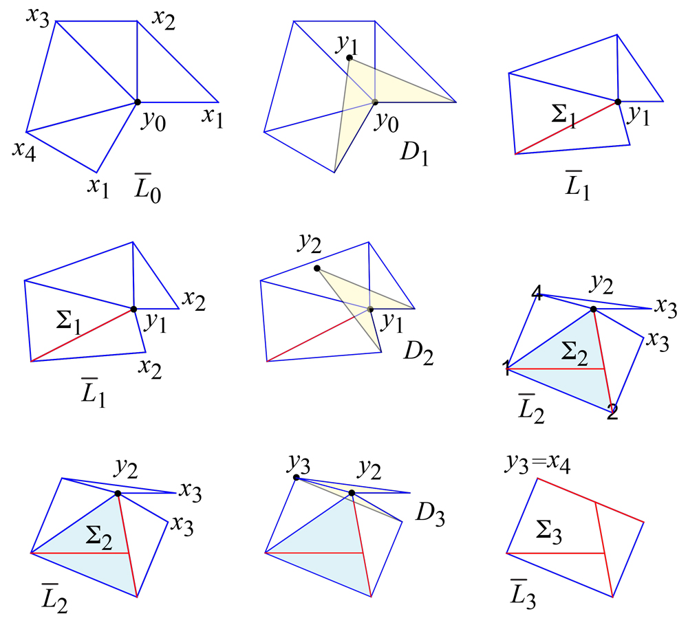
Figure 5.2: $P_{2}$. $X$ is a rectangle. Cf. Fig. 4.9(b).

We should emphasize that any one of these figures could be cut out and closed to a cone. This cone would not be rigid, and its boundary $\partial X$ would not (in general) be planar, as we mentioned earlier.

As a last example, we extract one row illustrating removal of $D_{5}$ from a pyramid of degree-$12$ in Fig. 5.3. We will refer to this figure subsequently.

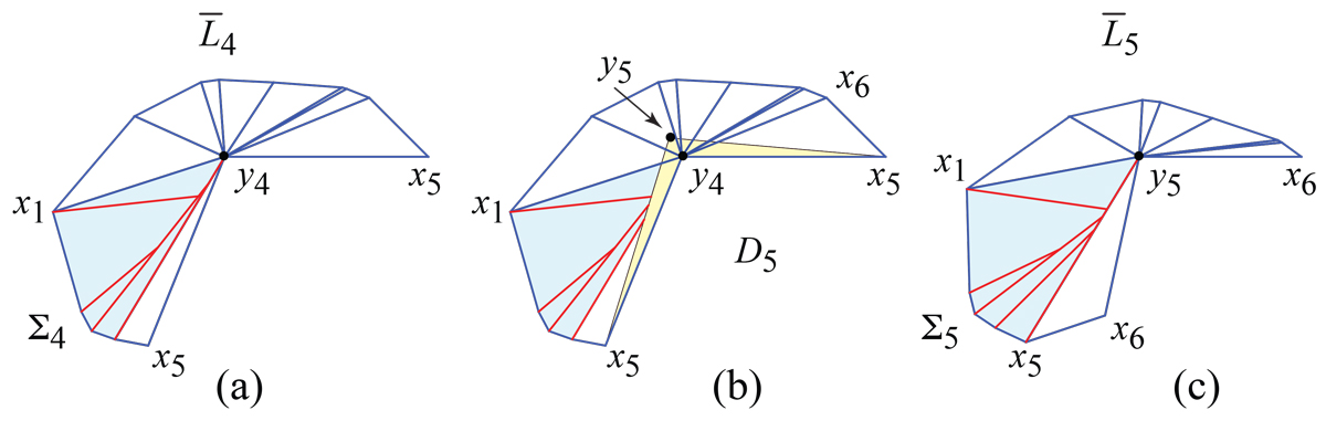
Figure 5.3: Pyramid of $n{=}12$ base vertices $x_{i}$. (a) $\bar{L}_{4}$. $S_{4}$ (blue). (b) Digon $D_{5}$ (yellow). (c) $\bar{L}_{5}$. ${\Sigma}_{i}$ in red.

5.4 Preliminary Lemmas

The viewpoint just described is simple enough to be implemented, and to allow us to construct the seal graph ${\Sigma}$ for any pyramid $P$. See ahead to Fig. 5.8 for examples. This leads to Theorem 5.3: ${\Sigma}$ is a tree. The proof of this claim is somewhat intricate, and presented in Section 5.5. That proof requires two lemmas, both involving the structure of the cut locus, which we present first. The reader might skip these proofs until later.

Lemma 5.1.

After removing digons $D_{1},\ldots,D_{i}$ and closing seals ${\sigma}_{1},\ldots,{\sigma}_{i}$, $C(x_{i+1},P_{i})$ includes the path $x_{1},\ldots,x_{i}$, with each node in that path of degree-$2$.

For example, in Fig. 5.3, $i=4$ and $C(x_{5},P_{4})$ includes $x_{1},x_{2},x_{3},x_{4}$.

Proof.

We start with the leaf $x_{i}\in C(x_{i+1})$, and argue that $(x_{i},x_{i-1},\ldots,x_{1})$ is a path ${\rho}$ in $C(x_{i+1})$, i.e., that every point along ${\rho}$ is of degree $\leq 2$. The proof uses techniques detailed in the proof of Lemma 4.3. In particular, Fig. 5.4 below depicts the situation abstractly, similar to Fig. 4.4 in Lemma 4.3.

First, $x_{i}$ is of degree-$1$ in $C(x_{i+1})$: The pyramid edge $x_{i+1}x_{i}$ is the shortest geodesic, unaffected by the digon removals up to $D_{i}$. An edge $e_{i}$ of $C(x_{i+1})$ starts at $x_{i}$, and because of the equal angles above on $L_{i}$ and below on $X$ at $x_{i}$, and because $e_{i}$ is bisecting, initially it starts along the geodesic $x_{i}x_{i-1}$. It then either continues to $x_{i-1}$, or reaches a ramification point.

Suppose the path continues $x_{i},x_{i-1},\ldots,x_{j}$, but then reaches a ramification point $r$ on $x_{j}x_{j-1}$. Let ${\rho}_{j}$ denote this path up to $r$. We now analyze this situation and show it is contradictory. Consult Fig. 5.4 throughout.

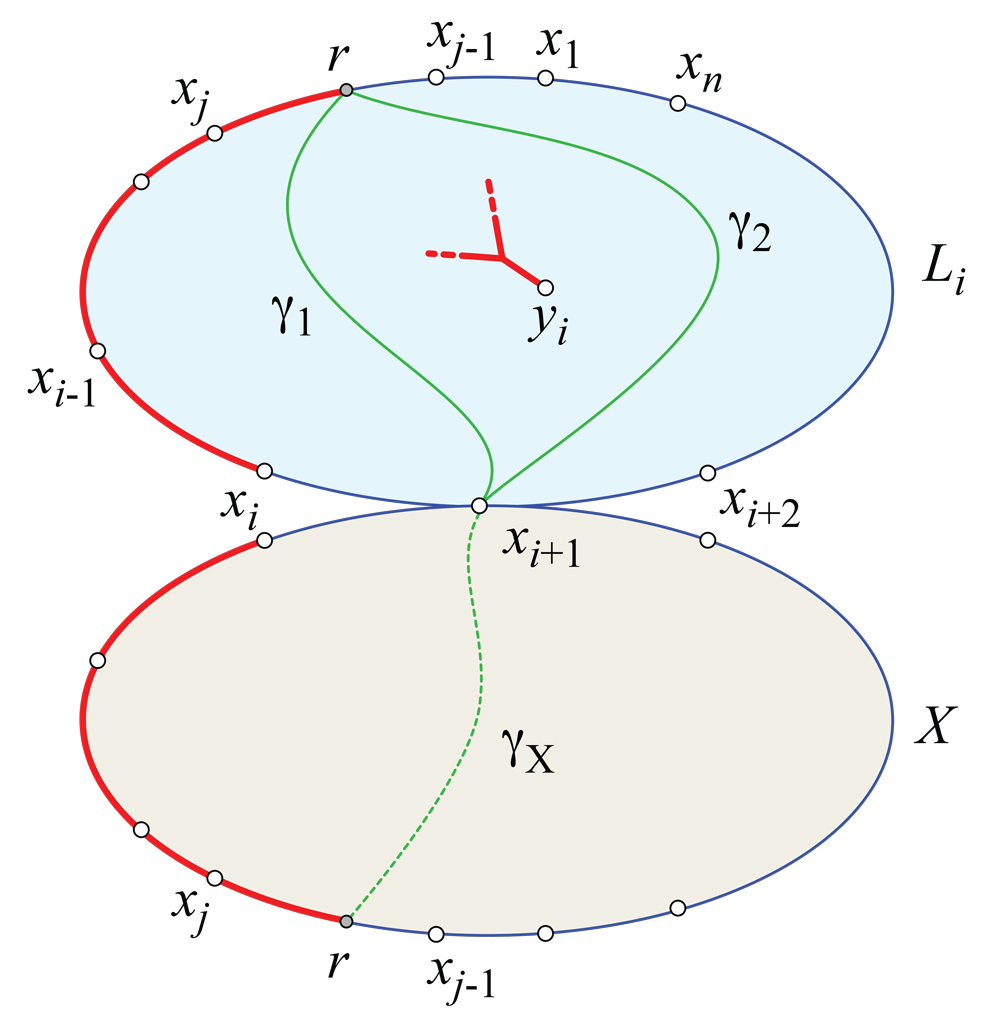
Figure 5.4: Abstract depiction of $x_{i},x_{i-1},\ldots,x_{1}$ path in $C(x_{i+1})$ (red). $X$ is flipped below; $L_{i}$ above.

The possible geodesics from $x_{i+1}$ to $r$ are: ${\gamma}_{X}$ on $X$ below, ${\gamma}_{1}$ and ${\gamma}_{2}$ on $L_{i}$ above, and possibly ${\gamma}_{3}$ both above and below. Note that there can only be the two ${\gamma}_{1}$ and ${\gamma}_{2}$ because there is just one vertex $y_{i}$ on $L_{i}$.

First consider ${\gamma}_{1}$, which, together with ${\gamma}_{X}$, encloses ${\rho}_{j}$. The planar convex chain along ${\rho}_{j}$, $x_{i},x_{i-1},\ldots,x_{j},r$ is congruent above and below, because the angles above and below are equal after digon removals. Thus the chords connecting the endpoints of the chains are equal, and so $|{\gamma}_{1}|=|{\gamma}_{X}|$.

Next consider ${\gamma}_{2}$, which, together with ${\gamma}_{X}$, encloses $x_{i+2},\ldots,x_{n},x_{1},\ldots,x_{j-1}$. We again compare the planar convex chain with angles below on $X$ to the chain with angles above on $L_{i}$. Because some of the angles above are strictly larger than their counterparts below, we can apply Cauchy’s Arm Lemma just as we did in the proof of Lemma 4.3(Claim (1)) to conclude that $|{\gamma}_{2}|>|{\gamma}_{X}|$. Therefore ${\gamma}_{2}$ cannot add to the degree of $r$ in $C(x_{i+1})$.

Finally, a geodesic ${\gamma}_{3}$ that lies on both $L_{i}$ and $X$ must have a portion completely above on $L_{i}$, to which we may apply the same arm-lemma argument to conclude that $|{\gamma}_{3}|>|{\gamma}_{X}|$.

Therefore, $r$ is in fact of degree $2$, it is not a ramification point, and ${\rho}$ extends from $x_{i}$ to $x_{1}$ as claimed. ∎

Lemma 5.2.

Assume the digons $D_{1},\ldots,D_{i}$ have been removed and $S_{i-1}$ is the sealed region containing ${\sigma}_{1},\ldots,{\sigma}_{i-1}$ (this inclusion will be proven later). Let $a_{i}$ be the first ramification point of $C(x_{i},P_{i-1})$, on the segment $y_{i-1}a_{i}$. Then $a_{i}\not\in S_{i-1}$.

First we illustrate the claim of the lemma with the example from Fig. 5.3(b), repeated as Fig. 5.5(a). In order for the lemma to be false, the situation instead must appear as in (b) of the figure, with $a_{5}\in S_{4}$.

Proof.

For the purposes of contradiction, consider the situation depicted abstractly in Fig. 5.5(c), with $a_{i}\in S_{i-1}$. By Lemma 5.1, $x_{1},\ldots,x_{i-1}$ is a path of degree-$2$ nodes in $C(x_{i},P_{i-1})=C(x_{i})$. The edge $y_{i-1}a_{i}$ of $C(x_{i})$ bisects the angle formed by the two images of $x_{i}$. From $a_{i}$, $C(x_{i})$ must contain a path ${\rho}$ that connects to $x_{i}$. Because $a_{i}\in S_{i-1}$, ${\rho}$ must start with an edge to the right of the line containing $y_{i-1}a_{i}$.

Note that $y_{i-1}$ is the only vertex on $L_{i-1}$, so $a_{i}$ is not a vertex, and therefore has a total surface angle ${\theta}_{a_{i}}=2\pi$. Lemma 2.3 requires a strictly leftward branch at $a_{i}$, left of the line containing $y_{i-1}a_{i}$. Call the path continuing this left branch $\lambda$. This path $\lambda$ is “trapped”: It cannot terminate in the interior of $S_{i-1}$ because there are no vertices in that region. It cannot connect to any one of $x_{1},\ldots,x_{i-1}$ because those nodes are degree-$2$. If $\lambda$ crossed ${\rho}$ it would form a cycle. Therefore we have reached a contradiction, and so $a_{i}\not\in S_{i-1}$. ∎

Figure 5.5: (a) Fig. 5.3(b). (b) How a counterexample might appear. (c) Abstract counterexample. Portions of $C(x_{i})$ purple.

5.5 Pyramid Seal Graph is a Tree

Roughly, we prove in this section that the complete seal graph ${\Sigma}={\Sigma}_{n}$, and intermediate seal graphs ${\Sigma}_{i}$, have the structure of a spiraling tree. Spiral trees—slit trees rather than seal trees—will play a significant role in Part II.

We repeat some notation here for convenience. The sealed region $S_{i}$ is bounded by the segments $x_{1}y_{i}$, $x_{i}y_{i}$, and the portion of $\partial X$ from $x_{1}$ to $x_{i}$. Also recall that each seal $\bm{{\sigma}}_{j}=(x_{j},y_{j})$ is directed from $x_{j}$ to $y_{j}$. The seal graph ${\Sigma}_{i}$ is composed of segments $s_{j}$, each a subsegment of ${\sigma}_{j}$.

Theorem 5.3.

The seal graph ${\Sigma}_{i}$, after removal of digons $D_{1},\ldots,D_{i}$ in counterclockwise order, has the following properties:

1. ${\Sigma}_{i}\subset S_{i}$.

2. ${\Sigma}_{i}$ is a directed tree with root $y_{i}$.

3. Each segment $s_{j}$ of ${\Sigma}_{i}$ is a (possibly truncated) seal ${\sigma}_{j}=x_{j}y_{j}$ that remains anchored on its $x_{j}$ endpoint; i.e., the truncation is on the $y_{i}$-end.

4. Each leaf $x_{j}$ is the start of a directed, convex path $\bm{\pi}_{j}$ to the root $y_{i}$.

5. The edges of $\bm{\pi}_{j}$ are portions of seal segments of increasing indices.

6. Along $\bm{\pi}_{j}$, lower-indexed edges terminate from the left on higher-indexed edges.

7. The last seal, $\bm{{\sigma}}_{i}=x_{i}y_{i}$, the root segment of ${\Sigma}_{i}$, has no segments of ${\Sigma}_{i}$ incident to its right side.

The last segment of the complete seal graph ${\Sigma}={\Sigma}_{n}$ coincides with the edge $x_{n-1}x_{n}$ of $\partial X$.

We again refer to Fig. 5.3(ab). When $i=4$, ${\Sigma}_{4}$ satisfies the properties, and we seek to re-establish the properties for ${\Sigma}_{5}$ in (c) of the figure. We enlarge (b) of that figure in Fig. 5.6 to track in this proof. It may also help to consult the complete seal graphs in Fig. 5.8.

Figure 5.6: $i=4$, before removal of digon $D_{i+1}=D_{5}$. Detail from Fig. 5.3(b).

Proof.

Induction Basis. These claims are trivially true for $i=0$ because ${\Sigma}_{0}=\varnothing$. So assume $i=1$. $L_{1}$ has just had the digon $D_{1}=x_{1}y_{1}$ excised around $y_{0}$. $\bar{L}_{1}$ is then cut open along $x_{2}y_{1}$. ${\Sigma}_{1}$ is the single segment ${\sigma}_{1}=x_{1}y_{1}$, and all properties are easily verified.

Induction Hypothesis. Assume that all properties hold for ${\Sigma}_{i}$. The removal of digon $D_{i+1}=x_{i+1}y_{i+1}$ leads to ${\Sigma}_{i+1}$. Now we establish the properties for ${\Sigma}_{i+1}$.

1. ${\Sigma}_{i+1}\subset S_{i+1}$. $S_{i+1}$ grows on both sides: by the triangle $x_{1}y_{i}y_{i+1}$ (clockwise in Fig. 5.6), and to $x_{i+1}y_{i+1}$ (counterclockwise in the figure). By Lemma 5.2, we know that $a_{i+1}\not\in S_{i}$, and because $y_{i+1}$ is on the $y_{i}a_{i+1}$ segment of $C(x_{i+1})$, we know that $y_{i+1}\not\in S_{i}$. Therefore the triangle $x_{1}y_{i}y_{i+1}$ does in fact grow $S_{i}$ on the $x_{1}$-end. On the $x_{i+1}$-end, the new seal $\bm{{\sigma}}_{i+1}=x_{i+1}y_{i+1}$ is incorporated, and all seal segments right of $\bm{{\sigma}}_{i+1}$ are clipped by the removal of digon $D_{i+1}$. Therefore indeed $S_{i+1}$ expands to include all of ${\Sigma}_{i+1}$.

2. ${\Sigma}_{i+1}$ is a directed tree with root $y_{i+1}$. We know that ${\Sigma}_{i}$ is a directed tree with root $y_{i}$. We first argue that the seal $\bm{{\sigma}}_{i+1}$ intersects the segments of ${\Sigma}_{i}$ from right-to-left, re-establishing property (7). Let ${\gamma}_{1}$ and ${\gamma}_{2}$ be the left and right geodesics of digon $D_{i+1}=x_{i+1}y_{i+1}$. ${\gamma}_{1}$ starts within the triangle $\triangle=x_{i}x_{i+1}y_{i}$, at an angle $({\alpha}_{i+1}+{\beta}_{i+1})/2$ left of the $x_{i+1}y_{i}$ edge of $\triangle$. Therefore ${\gamma}_{1}$ cuts into $S_{i}$ through the $x_{i}y_{i}$ edge of $\triangle$. The segments of ${\Sigma}_{i}$ crossed and clipped by ${\gamma}_{1}$ are crossed from right-to-left. And since $i+1$ is the highest indexed seal, the segments of ${\Sigma}_{i}$ that meet $\bm{{\sigma}}_{i+1}$ satisfy property (7): lower-indexed segments terminate on the left of $\bm{{\sigma}}_{i+1}$. Henceforth, we use ${\sigma}_{i+1}$ as determined by ${\gamma}_{1}$.

   By property (8), $\bm{{\sigma}}_{i}=x_{i}y_{i}$ is the root segment of ${\Sigma}_{i}$, which we now know is crossed by $\bm{{\sigma}}_{i+1}$ right-to-left, say crossing at point $p$. Because $y_{i+1}\not\in S_{i}$ by Lemma 5.2, $\bm{{\sigma}}_{i+1}$ has the root $y_{i}$ of ${\Sigma}_{i}$ to its right, and all the leaves $x_{j}$ of ${\Sigma}_{i}$ to its left.

   Now suppose ${\Sigma}_{i+1}$ has an undirected cycle $\Phi$; see Fig. 5.7. Because ${\Sigma}_{i}$ has no cycle, any cycle in ${\Sigma}_{i+1}$ must have one edge a subsegment of ${\sigma}_{i+1}$. Because all of ${\Sigma}_{i}$ right of $\bm{{\sigma}}_{i+1}$ is removed, the cycle $\Phi$ must “rest on” the left side of $\bm{{\sigma}}_{i+1}$. It is clear $\Phi$ cannot rest on the $x_{i+1}p$ portion of $\bm{{\sigma}}_{i+1}$. So $\Phi$ must rest on the portion of $\bm{{\sigma}}_{i+1}$ left of $\bm{{\sigma}}_{i}$, as illustrated. But then, imagining removing $\bm{{\sigma}}_{i+1}$, $\Phi$ must have formed a cycle $\Phi^{\prime}\supset\Phi$ in ${\Sigma}_{i}$, a contradiction. Therefore ${\Sigma}_{i+1}$ is indeed a tree.

   The remaining properties are now easily established.

3. Because $\bm{{\sigma}}_{i+1}$ clips segments of ${\Sigma}_{i}$ to its right, each segment $s_{j}\in{\Sigma}_{i}$ remains anchored on $x_{j}$. And the new segment $\bm{{\sigma}}_{i+1}$ is anchored on $x_{i+1}$.

4. The directed, convex path $\bm{\pi}_{j}$ remains, but now may by shortened where it joins with $\bm{{\sigma}}_{i+1}$.

5. The segments along $\bm{\pi}_{j}$ have increasing indices, possibly now including $i+1$.

6. We earlier established that lower-indexed segments of ${\Sigma}_{i+1}$ terminate from the left on higher-indexed segments, possibly now including $\bm{{\sigma}}_{i+1}$.

7. The last and new seal $\bm{{\sigma}}_{i+1}=x_{i+1}y_{i+1}$ becomes the root segment incident to the root $y_{i+1}$, and has no segments incident to its right side.

Finally, it is a consequence of Lemma 4.2 and the rigidity Theorem 2.9 that $y_{n-1}=x_{n}$ so that the $(n{-}1)$-st seal coincides with the edge $x_{n-1}x_{n}$. ∎

Figure 5.7: Cycle $\Phi$ is not possible: removing ${\sigma}_{i+1}$ extends $\Phi$ to $\Phi^{\prime}$.

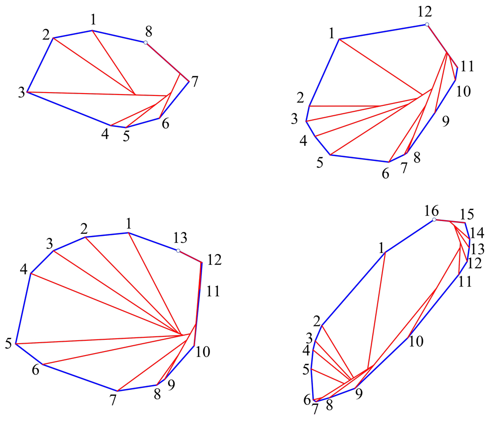
Figure 5.8: Four complete seal graphs.

5.5.1 Other Digon Orderings

The proof of Theorem 5.3 depends on removing the digons in the order $x_{1},x_{2},\ldots,x_{n-1}$ around $\partial X$. This affects Lemma 5.1’s conclusion that $x_{1},\ldots,x_{i}$ is a path in the cut locus, which then affects Lemma 5.2’s conclusion that the ramification point $a_{i+1}$ is outside the sealed region $S_{i}$. In addition, which side of the removal of digon $D_{i+1}$ clips ${\Sigma}_{i}$ is affected by knowing that $x_{i+1}$ is adjacent to $x_{i}$ on $\partial X$. All of these consideration affect the structure of the seal graph. We leave the question of whether the seal graph is a tree for other orderings of digon removals to Open Problem 18.3.

Toward this open problem, we only show here, with the next result, what a degree-$4$ vertex in ${\Sigma}$ must look like.

In the proof below, we simplify the notation of $\tilde{{\sigma}_{i}}$ on the base to just ${\sigma}_{i}$, keeping in mind that ${\sigma}_{i}$ and ${\sigma}_{j}$ formally live in different spaces,.

Lemma 5.4.

If a seal graph ${\Sigma}$ for a pyramid $L$ has a degree-$4$ vertex $z$, then there exist $i<j<k$ such that ${\sigma}_{i}$ and ${\sigma}_{j}$ end at $z$, and ${\sigma}_{k}$ passes beyond $z$. Moreover, the digon excision order is $D_{k}$ immediately after $D_{j}$ immediately after $D_{i}$.

Proof.

Consider a common point $z$ of ${\sigma}_{i}$ and ${\sigma}_{j}$, with $i<j$. We may assume $j>i+1$ , since otherwise $\deg z=3$ in ${\Sigma}$.

Assume first that no other ${\sigma}_{k}$ passes through $z$. Assume that $\deg z=4$ in ${\Sigma}$. This implies that the digon $D_{j}$ crosses ${\sigma}_{i}$ and, since ${\sigma}_{i}$ remains a geodesic after the excision of $D_{j}$, ${\sigma}_{i}$ must be orthogonal to both geodesics bounding $D_{j}$. Therefore, ${\sigma}_{i}$ creates with those two geodesics two geodesic triangles, both of positive curvature. So each such triangle contains a vertex inside, contradicting that $D_{j}$ itself contains only one vertex.

Assume now that ${\sigma}_{i}$ ends at $z$, as does ${\sigma}_{k}$ for some $k\not\in\{i,j\}$. Notice that we cannot have four ${\sigma}$s ending at $z$, because for the last one arriving—say ${\sigma}_{k}$—${\sigma}_{k}$ would create a vertex at $z$, which will be excised by the digon $D_{k+1}$, breaking that degree-$4$ configuration at $z$.

So we may assume that $z$ belongs only to ${\sigma}_{i}$, ${\sigma}_{j}$, and ${\sigma}_{k}$. We may further assume, without loss of generality, that $i<j<k$.

Notice that both ${\sigma}_{i}$ and ${\sigma}_{j}$ end at $z$ and ${\sigma}_{k}$ does not, because otherwise ${\sigma}_{k}$ would create a vertex on ${\sigma}_{i}$ (or on ${\sigma}_{j}$) which would be excised by the digon $D_{k+1}$, breaking that degree-$4$ configuration at $z$.

The digon excision order follows: only $D_{j}$ could surround $y_{i}$, so its excision was just after $D_{i}$, and similarly for $D_{j}$. ∎

For a particular digon-removal ordering, consider the inverse image of ${\Sigma}$ on $L$, and denote it by $\chi$. $\chi$ is a simple geodesic polygon surrounding $v$. In Fig. 4.11(a), $\chi$ is the boundary of the gray region, effectively the union of the digons (but recall that the digons $D_{i}$ live on different surfaces $P_{i-1}$; hence “effectively”). Clearly, excising the surface bounded by $\chi$ from $L$ all at once achieves the same effect as excising the digons $D_{i}$ one-by-one.

The region of $L$ bound by a geodesic polygon $\chi$ is a particular instances of what we call a crest: a subset of $L$ enclosing $v$ whose removal and suitable suturing via AGT will reduce $L$ to $X$. Note that we allow the boundary of a crest to include portions of $\partial L$, e.g., $\chi$ in Fig. 4.11(a) includes the $x_{i}$ as well as the edge $x_{5}x_{6}$. In Chapter 7 we will show that it is possible to construct crests directly on $L$ without deriving them from digon removals.

Chapter 6 Algorithm for Tailoring via Sculpting

In this research we have also concentrated on achieving constructive proofs of the theorems, constructive in the sense of leading to finite algorithms. In this chapter we follow Theorem 4.6 to yield an algorithm for achieving the tailoring of $P$ to $Q$. Throughout we measure computational complexity in terms of $n$, where $n=\max\{|P|,|Q|\}$ is the number of vertices of the larger of $P$ or $Q$; so $|P|,|Q|=O(n)$. Our goal for all the algorithms is to achieve polynomial-time complexity, $O(n^{k})$, but we have not worked hard to lower $k$, through, e.g., exploitation of efficient data structures. Instead we are content to leave improvements for future work. We will see that $k=4$ seems to suffice.

Euler’s $V{-}E{+}F$ theorem implies that the number of edges and faces of a polyhedron are linearly related to the number of vertices, so all components of $P$ and $Q$ are $O(n)$. Thus for tailoring via slicing, the number of slices of $P$ is $O(n)$: one slice per face of $Q$. Each slice leads to g-domes, each g-dome to pyramids, and each pyramid is reduced to its base by a series of tailoring steps: digon excisions and suturings.

We analyze the complexity in four parts, the $0$-th just the conceptual slicing of $P$ by planes on each face of $Q$:

• Algorithm 0: Slice $P$ to $Q$: $O(n)$.

• Algorithm 1: slice $\to$ g-domes, following Lemma 4.1.

• Algorithm 2: g-dome $\to$ pyramids, following Theorem 3.2.

• Algorithm 3: pyramid $\to$ digons, following Lemma 4.4.

Algorithms $0,1,2$ operate on the extrinsic $3$-dimensional structure of the polyhedra. Algorithm $3$ instead processes its calculations on the intrinsic structure of the surface.

6.1 Algorithm 1: slice$~{}\to~{}$g-domes

Input : One slice plane $\Pi$

Output : $O(n)$ g-domes, a total of at most $O(n)$ vertices.

// Consult Fig. 4.1.

Let $F$ be the face of $Q$ lying in $\Pi$, and $e$ be an edge of $F$.

Sort vertices angularly about $e$. // $O(n\log n)$

for $i=0,1,2,\ldots,k$ do

      

      Rotate $\Pi_{i}$ about $e$ until the portion swept is not a g-dome.

      // Following Lemma 4.1.

      

      Add to g-domes list.

end for

Result: List of $O(n)$ g-domes.

Algorithm 1 From one slice, $O(n)$ g-domes.

Algorithm 1 follows the proof of Lemma 4.1, which clearly results in at most $O(n)$ g-domes, with the sum of the complexities of the g-domes for any one slice $O(n)$. It can be implemented to run in $O(n\log n)$ time. Therefore, over $O(n)$ slices, each resulting in $O(n)$ g-dome vertices, we have at most $O(n^{2}\log n)$ total g-dome complexity: $O(n\log n)$ sorting repeated $O(n)$ times.

However, it could be that a clever choice of ordering of the slices always results in a smaller total complexity, perhaps $O(n\log n)$. Using ${\Omega}$ to indicate a lower bound, the question is: Might each of the ${\Omega}(n)$ slices from Algorithm $0$ lead to g-domes with a total complexity of ${\Omega}(n^{2})$, independent of the order of slicing? Although resolving this question has only a small effect on the overall time-complexity of the tailoring algorithm, we take a detour to explore this issue via an example in the next subsection.

6.1.1 Complexity of sculpting

Example 6.1.

Consider Fig. 6.1, two nested pyramids $Q\subset P$ sharing a common regular polygon base. The combinatorial complexity of slicing $P$ with face planes of $Q$ is order-sensitive: from ${\Omega}(n^{2})$ to ${\Omega}(n\log n)$.

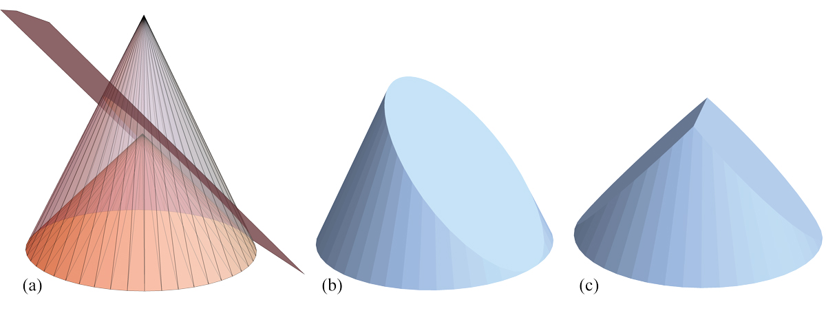
Figure 6.1: $Q\subset P$. The shared base is a regular polygon of $n{=}48$ sides. (a) One slice-plane $\Pi_{0}$ lying on a face of $Q$. (b) After slicing by $\Pi_{0}$. (c) A second, opposite slice $\Pi_{n/2}$.

Proof.

Let the faces of $Q$ ordered in sequence around the base be $F_{0},F_{1},\ldots,F_{n-1}$, each $F_{i}$ determining a plane $\Pi_{i}$. Let $P_{i}$ be the polyhedron after slicing $P$ with planes $\Pi_{0},\Pi_{1},\ldots,\Pi_{i}$. $\Pi_{0}$ cuts $n-2$ edges of $P$, as shown in Fig. 6.1(a,b), and effectively removes half the edges of $P$ from later slices. If $P$ is sliced in the order $i=1,2,\ldots,n-2$, following adjacent faces around the base, each plane cuts a diminishing number of the remaining edges. An explicit calculation shows that plane $\Pi_{i}$ cuts $\lfloor\frac{n+1-i}{2}\rfloor$ edges of $P_{i-1}$. And because

$$\sum_{i=1}^{n-2}\left\lfloor\frac{n+1-i}{2}\right\rfloor=\Omega(n^{2})\;,$$

with this plane-slice ordering, ${\Omega}(n)$ slices each have ${\Omega}(n)$ vertices, for a total quadratic complexity, ${\Omega}(n^{2})$.

However, if one instead orders the slices in a binary-search pattern, then the total complexity is ${\Omega}(n\log n)$, as we now show. Let $n=2^{m}$ be a power of $2$ without loss of generality. The pattern is slicing with planes lying on faces $F_{i}$ with indices in the order

$$s=\left(0,\frac{n}{2},\frac{n}{4},\frac{3n}{4},\frac{n}{8},\frac{3n}{8},\frac{5n}{8},\frac{7n}{8},\ldots\right)\;.$$

We partition this sequence $s$ of indices into subsequences, $s=(0,s_{1},s_{2},\ldots,s_{m})$, as follows:

$$s_{1} = \left(\frac{n}{2}\right)$$

$$s_{2} = \left(\frac{n}{2^{2}},\frac{3n}{2^{2}}\right)$$

$$s_{3} = \left(\frac{n}{2^{3}},\frac{3n}{2^{3}},\frac{5n}{2^{3}},\frac{7n}{2^{3}}\right)$$

$$\cdots$$

$$s_{k} = \left(\frac{j\,n}{2^{k}}\right),\;\textrm{where}\;j=1,3,5,\ldots,2^{k}{-}1\;.$$

Notice that the number of indices in sequence $s_{k}$, $|s_{k}|=2^{k-1}$. As a check, the total number of indices in $s$ is

$$1+\sum_{k=1}^{m}|s_{k}|=1+\sum_{k=1}^{m}2^{k-1}=2^{m}=n\;.$$

One can calculate that the slice at $\displaystyle{i=\frac{j\,n}{2^{k}}}$ only cuts $\displaystyle{\frac{n}{2^{k}}}$ edges of $P_{i-1}$. Only $\displaystyle{\frac{n}{2^{k-1}}}$ edges are “exposed” to $\Pi_{i}$: for example, for $k=2$ and $i=1/4$, $n/2$ edges are possibly available for cutting by $\Pi_{i}$, as can be seen in Fig. 6.1(c). However, because of the slant of $\Pi_{i}$, only half of those, $n/4$, are in fact cut by $\Pi_{i}$.

Now we compute the total number of edges sliced by the planes following the sequence $s$. Because $|s_{k}|=2^{k-1}$, and each slice in $s_{k}$ cuts $\displaystyle{\frac{n}{2^{k}}}$edges, the total number of cuts over all $k$ is

$$\sum_{k=1}^{m}2^{k-1}\frac{n}{2^{k}}=n\sum_{k=1}^{m}\frac{1}{2}=n\,\frac{m}{2}\;.$$

And since $m=\log n$, the total complexity is ${\Omega}(n\log n)$, or an average of ${\Omega}(\log n)$ for each of ${\Omega}(n)$ slices. ∎

In the absence of a resolution to this complexity question, we will assume that Algorithm 0 and Algoirthm 1 together result in $O(n)$ g-domes each of $O(n)$ vertices, produced in time $O(n^{2})$.

6.2 Algorithm 2: g-dome$~{}\to~{}$pyramids

Input : One g-dome $G$ of $O(n)$ vertices

Output : $O(n)$ pyramids, each of size $O(n)$; and $O(n^{2})$ pyramids, size $O(1)$.

// Following Theorem 3.2.

for each of $k=O(n)$ vertex-degree reductions do

      

      As in Theorem 3.2, slice with plane: $O(k)$.

      Remove pyramid $P$ of $O(k)$ vertices.

      “Clean-up” by removing $k$ pyramids each of size $O(1)$.

end for

Result: List of pyramids.

Algorithm 2 Partition one g-dome to $O(n)$ pyramids.

We follow Theorem 3.2 for partitioning each g-dome $G$ into pyramids. Each vertex $v_{i}$ of the top-canopy of $G$ is removed, as in Fig. 3.3, until only one remains. Removal of each $v_{i}$ follows the degree-removal steps illustrated in Fig. 3.4.

Because the sum of the vertex degrees of a g-dome is $2E=O(n)$, the asymptotic complexity of processing a g-dome with many vertices in its top-canopy is no different than it is for just two vertices as in Fig. 3.3. Moreover, we can assume that $v_{2}$ has degree-$3$ while $v_{1}$ has degree-$k$, with $k=O(n)$.

First a plane slice results in a pyramid of $k$ vertices with apex $v_{1}$, which is removed (and reduced by Algorithm 3). Next follows a “clean-up” phase that removes $O(k)$ pyramids each of $4$ or $5$ vertices, so of constant size, $O(1)$.

This is then repeated for the new apex of degree $k-1$: removal of a pyramid of $k-1$ vertices, and cleanup of $O(k-1)$ pyramids of constant size. After iterating through $k,k-1,k-2,\ldots$, the algorithm has sliced off $O(k^{2})$ pyramids of constant size, and $O(k)$ pyramids of size $O(k)$. In the worst case $k=O(n)$, for a total complexity of $O(n^{2})$.

6.3 Algorithm 3: pyramid$~{}\to~{}$digons

Input : A pyramid $P$ of $O(n)$ vertices

Output : $O(n)$ digons whose removal flattens $P$ to $X$.

// Following Lemma 4.4.

// Assume apex degree-$k$, with $k=O(n)$.

for each of $x_{i}$, $i=1,2,\ldots,k$ do

      

      Construct digon $D_{i}(x_{i},y_{i})$: Locate $y_{i}$.

      Locate $y_{i}$ by tracing geodesics: $O(k)$.

end for

Result: List of $O(n)$ digons

Algorithm 3 Tailor one pyramid $P$ to its base $X$.

Lastly we concentrate on the cost of removing one pyramid $P$ of $O(n)$ vertices. Following Lemma 4.4, this requires $O(n)$ digon removals. For each digon $D_{i}(x_{i},y_{i})$, we need to calculate the location of $y_{i}$ on $C(x_{i})$; then $y_{i}$ becomes a vertex for the removal of the next digon $D_{i+1}$. Fortunately, there is no need to compute the cut locus $C(x_{i})$.

Let us focus on locating $y_{i}$, after the removal of $D_{i-1}(x_{i-1},y_{i-1})$ the previous iteration. Recall that $y_{i}$ is the only vertex on $L_{i}$, so it is immediate to find the shortest path ${\gamma}$ from $x_{i}$ to $y_{i}$. We know the angle ${\theta}={\omega}_{Q}(x_{i})-{\omega}_{P}(x_{i})$ needed to be removed by $D_{i}$, so we know that geodesics ${\gamma}_{1}$ and ${\gamma}_{2}$ at angles ${\theta}/2$ left and right of ${\gamma}=x_{i}y_{i}$ will meet at $y_{i}$. Tracing ${\gamma}_{1}$ and ${\gamma}_{2}$ over the surface might cross sealed digons $D_{1},\ldots,D_{i-1}$, the blueseals ${\sigma}_{i}$ in Fig. 4.11(b). So the cost of computing ${\gamma}_{1}\cap{\gamma}_{2}=y_{i}$ is $O(n)$.

Thus the complexity of tailoring one pyramid of $O(n)$ vertices is $O(n^{2})$.

Note that we do not need the extrinsic $3$-dimensional structure of the intermediate polyhedra guaranteed by AGT to perform the calculations, as is evident in the example described in Fig. 4.11.

6.4 Overall Tailoring Algorithm

Putting the three algorithm complexities together, and for succinctness abbreviating $O(n)$ with $n$ and “time-complexity” with “complexity,” we have:

1. $n$ slices $\to$ $n$ g-domes, each of size $n$: complexity $n^{2}\log n$.

2. $1$ g-dome of size $n$ $\to$

   1. $n$ pyramids, each of size $n$: complexity $n^{2}$.

   2. $+$ $n^{2}$ constant-size pyramids: complexity $n^{2}$.

3. $1$ pyramid of size $n$ $\to$ $n^{2}$ to reduce to base: complexity $n^{2}$.

(1) and (2) together have complexity $n^{3}$, iterating over each of the $n$ domes. (The $n\log n$ sorting need not be repeated after the g-domes are identified.) (3) repeats $n^{2}$ over (potentially) $n^{2}$ pyramids: $n$ g-domes resulting in $n$ pyramids each. Thus the total complexity is $n^{4}$. We summarize in a theorem:

Theorem 6.2.

Given convex polyhedra $P$ and $Q$ of at most $n$ vertices each, and $Q\subset P$, $P$ can be tailored to $Q$, tracking a sculpting of $Q$ from $P$ as in Theorem 4.6, in time $O(n^{4})$.

Chapter 7 Crests

In this chapter we revisit the suggestion made at the end of Chapter 5 that the digons to reduce one pyramid to its base could be cut out all at once. As before, let $P=L\cup X$ be a pyramid with base $X$ and lateral sides $L$. Recall that a crest is a subset of $L$ enclosing $v$ whose removal and suitable suturing via AGT will reduce $L$ to $X$.

We derive a method for identifying a crest that does not rely on digon removals, but rather works directly on a pyramid. This allows us to achieve in Theorem 7.5 reshaping of $P$ to $Q$ by the removal of crests to flatten pyramids. We call this process crest-tailoring, in contrast to the digon-tailoring explored in Chapter 4. It represents a tradeoff between the simplicity of digons and the number of excisions: for digon-tailoring, $O(n)$ per pyramid, for crests, one per pyramid. We first illustrate the process of identifying a crest on two example pyramids before proving that it always works.

7.1 Examples

Let $P=L\cup X$ with $\partial X=\partial L=(x_{1},x_{2},\ldots,x_{k})$ having vertices $x_{i}$. The apex is $v$, which projects orthogonally to $\bar{v}$. We will describe the procedure for identifying a crest first for $\bar{v}\in X$ and then for $\bar{v}\not\in X$. Although the cases initially feel different, the proofs will show that they are nearly the same.

Fig. 7.1 illustrates the case $\bar{v}\in X$. Let $T_{i}=x_{i}x_{i+1}v$ and $\bar{T}_{i}=x_{i}x_{i+1}\bar{v}$. We proved in Lemma 2.8 that the angle $\bar{{\theta}}_{i}$ at $x_{i}$ in $X$ is strictly smaller than than the angle ${\theta}_{i}$ on $L$, the sum of the angles in $T_{i-1}$ and $T_{i}$ incident to $x_{i}$ (as long as $|v\bar{v}|>0$).

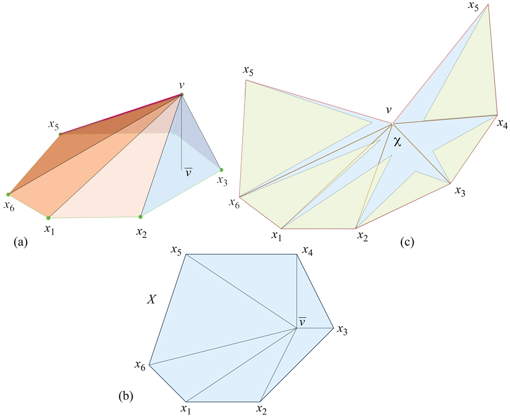
Figure 7.1: (a) Pyramid. (b) $X$ with projected triangles $\bar{T}_{i}=x_{i}x_{i+1}\bar{v}$. (c) Flattening of $L$ to $\bar{L}$, in this case by cutting the edge $x_{5}v$. The lifted triangles $T^{L}_{i}$ are shown yellow. The crest $\chi$ is blue.

A key definition is the lift of $\bar{T}_{i}$ onto $L$. Let $\bar{{\alpha}}_{i}$ and $\bar{{\beta}}_{i}$ be the base angles of $\bar{T}_{i}$, at $x_{i}$ and $x_{i+1}$ respectively. On $L$, extend geodesic ${\gamma}_{i}$ from $x_{i}$ at angle $\bar{{\alpha}}_{i}$, and extend geodesic ${\gamma}_{i+1}$ from $x_{i+1}$ at angle $\bar{{\beta}}_{i}$. Let $v_{i}$ be the point on $L$ at which these geodesics meet; $v_{i}$ is the image of $\bar{v}$. (We will not establish that indeed these geodesics meet on $L$ until Lemma 7.3.) Then $\operatorname{lift}(\bar{T}_{i})=T^{L}_{i}$ is a geodesic triangle on $L$ isometric to $\bar{T}_{i}$. Another way to view the lift of $\bar{T}_{i}$ is to imagine $\bar{T}_{i}$ rotating about $x_{i}x_{i+1}$ by the dihedral angle there and pasting it on the inside of $L$.

Yet another way to view the lift is as follows. $L$ is isometric to a cone and can be flattened by cutting along a generator, i.e., a segment from $v$ to $\partial L$. Let $\bar{L}$ be a particular flattening, with the cut generator not “near” $x_{i}$ just for simplicity. Then place a copy of $\bar{T}_{i}$ on $\bar{L}$ matching $x_{i}x_{i+1}$. Then refold $\bar{L}$ to $L$. We will continue to reason with a flattened $\bar{L}$ but remembering that $\bar{L}$ is a representation of $L$, and so the cut edge is not relevant.

This last layout-viewpoint yields a method to construct a full crest, call it $\chi$. The base $X$, partitioned into $\bar{T}_{i}$, can be modified by opening the angle at $x_{i}$ from $\bar{{\theta}}_{i}$ to ${\theta}_{i}$. After opening at all $x_{i}$, this figure can be superimposed on the flattened $\bar{L}$, matching the boundaries $x_{1},\ldots,x_{k}$. This is illustrated in Fig. 7.1(c). The crest is then the portions of $L$ not covered by the lifted $\bar{T}_{i}$. It should be clear that cutting out $\chi$ and suturing closed the matching edges will reduce $L$ to $X$, for the $\bar{T}_{i}$ remaining after removing $\chi$ exactly partition $X$.

We next illustrate the case when $\bar{v}\not\in X$; see Fig. 7.2. We perform the exact same process of lifting triangles $\bar{T}_{i}$ to $L$, but we clip those triangles to $X$—i.e., form the polygon $\bar{T}_{i}\cap X$—as indicated in (c) of the figure. Notice that two triangles, $\bar{T}_{3}$ and $\bar{T}_{4}$, are removed by the clipping intersection. Again it should be clear that cutting out $\chi$ and suturing closed will reduce $L$ to $X$.

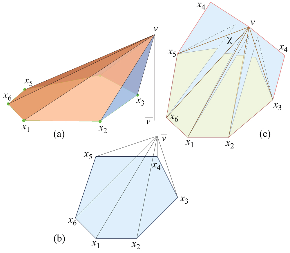
Figure 7.2: Following the same conventions as in Fig. 7.1: (a) Pyramid. (b) $X$; $\bar{v}\not\in X$. (c) $\bar{L}$, yellow clipped lifted triangles $T^{L}_{i}$, and blue crest $\chi$.

7.2 Proofs

We will need several geometric properties.

Let $\bar{{\theta}}_{i}$ be the angle at $x_{i}$ in $X$, and ${\theta}_{i}$ the angle at $x_{i}$ on $L$, the sum of two triangle angles incident to $x_{i}$. Then, by Lemma 2.8, ${\theta}_{i}>\bar{{\theta}}_{i}$.

Lemma 7.1.

Let $T=abc$ be a triangle in $\mathbb{R}^{3}$, with $ab$ on plane $\Pi$ and $c$ above that plane. Let $\bar{c}$ be the orthogonal projection of $c$ onto $\Pi$, and $\bar{T}=ab\bar{c}$ the projected triangle. Finally, let $T^{r}=abc^{r}$ be the triangle $T$ flattened to $\Pi$ by rotating about $ab$. Then $c^{r}$ and $\bar{c}$ lie on the altitude line perpendicular to the line containing $ab$.

Proof.

See Fig. 7.3. The claim follows from the Theorem of the Three Perpendiculars. Note that $T^{r}$ is congruent to $T$. ∎

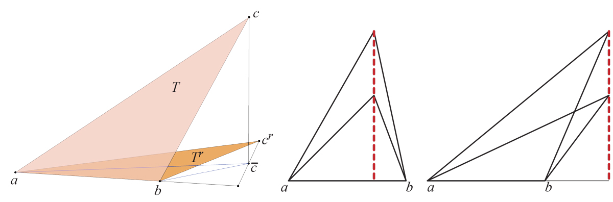
Figure 7.3: Rotated apex $c^{r}$ and projected apex $\bar{c}$ lie on same altitude.

The consequence of Lemma 7.1 is that, superimposing a lifted triangle $\bar{T}^{L}$ on a planar layout $\bar{L}$ of $L$, the images of $v$ in $\bar{L}$ and $\bar{v}$ of $\bar{T}$, lie along the altitude of $T$.

The following lemma assumes that $\bar{v}\in X$. The case when $\bar{v}\not\in X$ will be treated separately. Let $\bar{L}$ be a planar layout of $L$, say, cut open at edge $x_{1}v$. Let ${\tau}_{i}=\pi-({\beta}_{i-1}+{\alpha}_{i})=\pi-{\theta}_{i}$ be the turn angle at vertex $x_{i}$ in the layout. Because $\bar{v}\in X$, ${\tau}_{i}>0$, i.e., the planar image of $\partial L$ in $\bar{L}$ is a convex chain, and also convex wrapping around the cut edge $x_{1}v$.

Let $a_{i}$ be the segment altitude of triangle $T_{i}=x_{i}vx_{i+1}$ in the layout $\bar{L}$. Let $\nu=2\pi-{\omega}(v)$ be the surface angle of $P$ incident to $v$.

Lemma 7.2.

When $\bar{v}\in X$ and consequentially $\bar{L}$ is a convex chain $x_{1},\ldots,x_{k}$, the following hold (with $k+1\equiv 1\bmod{k}$):

1. The sum of the turn angles, $\sum_{i}{\tau}_{i}=\nu$, the surface angle incident to $v$.

2. The angle between $a_{i}$ and $a_{i+1}$ at $v$ on $L$ is exactly equal to the turn angle ${\tau}_{i}$ at vertex $x_{i}$.

3. The altitudes occur in order around $v$, in the sense that $a_{i+1}$ is counterclockwise of $a_{i}$ around $v$.

Proof.

1. Viewing the entire layout $\bar{L}$ as a simple polygon, $\sum_{i}{\tau}_{i}=2\pi$. But we need to distinguish between ${\tau}_{1}$ at the edge $x_{1}v$ cut to flatten $L$, and ${\tau}^{\prime}_{1}$, the turns at the two images of $x_{1}$ in $\bar{L}$:

   $${\tau}^{\prime}_{1}=2\pi-({\alpha}_{1}+{\beta}_{k})=\pi+{\tau}_{1}\;.$$

   The second anomalous turn in $\bar{L}$ is $\pi-\nu$ at $v$. So we have

   $${\tau}^{\prime}_{1}+\sum_{i=2}^{k}{\tau}_{i}+(\pi-\nu) = 2\pi\;,$$

   $$\sum_{i=1}^{k}{\tau}_{i} = \nu\;.$$

2. This can be seen by extending $T_{i}=x_{i}vx_{i+1}$ to a right triangle, with right angle at the foot of altitude $a_{i}$. See Fig. 7.4.

3. This follows directly from (b). Note that here we rely on the turns ${\tau}_{i}$ being positive, i.e., convex. See Fig. 7.5.

∎

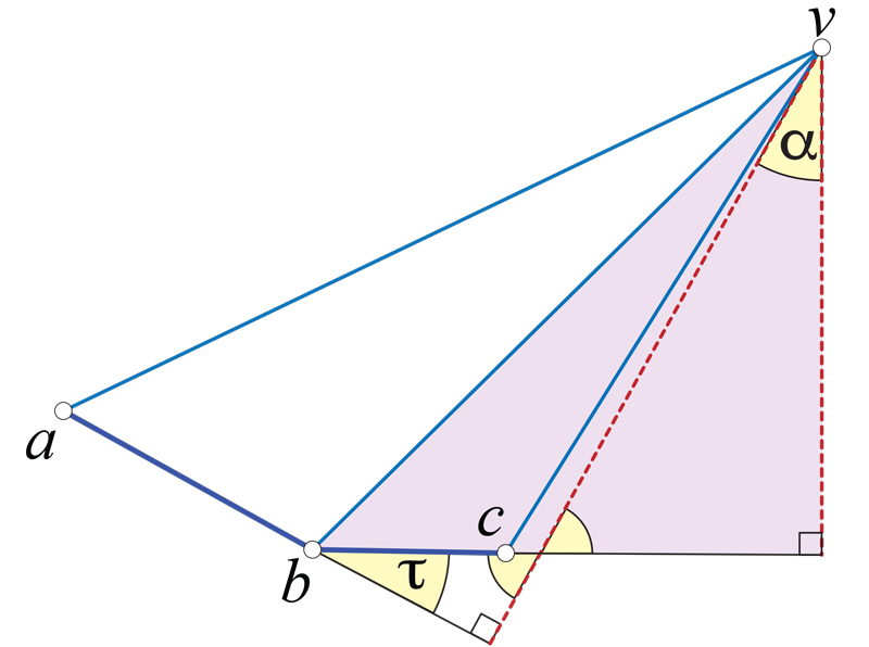
Figure 7.4: Triangles $avb$ and $bvc$ turn ${\tau}$ at $b$ of the convex chain $abc$. ${\tau}$ is equal to the altitude turn ${\alpha}$; angles of similar right triangles marked.

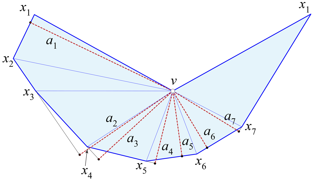
Figure 7.5: A convex chain $x_{1},\ldots,x_{7}$ and the corresponding altitudes $a_{1},\ldots,a_{7}$.

The consequence of Lemma 7.2 is that the surface angle $\nu$ around $v$ is partitioned by the altitudes $a_{i}$ in order, because $\sum_{i}{\tau}_{i}=\nu$, and the angle between $a_{i}$ and $a_{i+1}$ is ${\tau}_{i}$. Moreover, Lemma 7.1 shows that the apexes of each lifted triangle $\bar{T}^{L}_{i}$ lie on those altitudes, at some positive distance from $v$. Consequently, we can connect those apexes to form a simple geodesic polygon enclosing $v$ on $L$. Because every turn angle ${\tau}_{i}$ is strictly less than $\pi$, connecting two adjacent apexes along $a_{i}$ and $a_{i+1}$ will keep $v$ to the same (counterclockwise) side. Call this polygon the moat $M$ of $P$. Fig. 7.6 illustrates the moat for the example in Fig. 7.1(c).

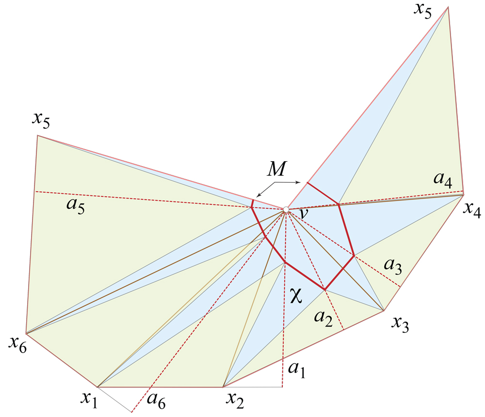
Figure 7.6: The layout from Fig. 7.1(c) shown with moat $M$ and altitudes $a_{i}$ identified.

Lemma 7.3.

For the case $\bar{v}\in X$, the lifting of all triangles $\bar{T}_{i}$ to $\bar{T}^{L}_{i}$ onto $L$ has the following properties, (where we shorten “geodesic triangle” to “triangle”):

1. Each lifted triangle $\bar{T}^{L}_{i}$ fits on $L$: $\bar{T}^{L}_{i}\subset L$.

2. $v$ does not lie in any triangle $\bar{T}^{L}_{i}$.

3. No lifted triangle self-overlaps, and no pair of triangles overlap.

Proof.

1. Because the apex of the lifted $\bar{T}^{L}_{i}$ is on the moat $M$ which surrounds $v$, $\bar{T}^{L}_{i}$ remains on the portion of $L$ outside the moat.

2. Therefore no $\bar{T}^{L}_{i}$ includes $v$.

3. If we view the overlay of $\bar{L}$ with the opening of $\partial X$ by the angle ${\theta}_{i}-\bar{{\theta}}_{i}$ at each $x_{i}$ image, as in Fig. 7.1(c), then Cauchy’s Arm Lemma shows that two lifted triangles cannot overlap. Suppose $\bar{T}^{L}_{i}$ and $\bar{T}^{L}_{j}$ overlap, $i<j$. Then we can identify two points $p_{i}\in\bar{T}^{L}_{i}$ and $p_{j}\in\bar{T}^{L}_{y}$ that coincide in the layout. But in $X$, $p_{i}$ and $p_{j}$ were separated by a positive distance $d=|p_{i}p_{j}|$. In $X$, draw a convex chain from $p_{i}$ to $\partial X$, around that boundary, to $p_{j}$. The layout opens this chain by the positive angles ${\theta}_{i}-\bar{{\theta}}_{i}$, and so in the layout, $p_{i}$ and $p_{j}$ must be separated further than $d$, a contradiction.

∎

Lemma 7.3 shows that $\chi$, the region of $L$ not covered by the lifted triangles, is indeed a crest.

We now turn to the case $\bar{v}\not\in X$. The difficulty here is that $\partial L$ in a layout $\bar{L}$ of $L$ may not be a convex chain, and Lemma 7.2 relies on convexity for the altitudes to connect to $v$ in the same order as the vertices around $X$. Indeed if $v$ were closer the plane of $X$ in the example in Fig. 7.2(a), then the angle at $x_{3}$ would be reflex. In general, a contiguous portion of $\partial L$ could be reflex. Lifting triangles incident to that reflex chain could lead to overlap, violating (c) of Lemma 7.3.

However, as described earlier in Fig. 7.2(c), the crest is formed by clipping the triangles $\bar{T}_{i}$ to $X$. Triangles $\bar{T}_{3}=x_{3}\bar{v}x_{4}$ and $\bar{T}_{4}=x_{4}\bar{v}x_{5}$ in Fig. 7.2(b) fall entirely outside $X$, and so play no role. The convex portion of $\partial L$ still satisfies Lemma 7.2, so the corresponding altitudes are incident to $v$ in the same order as the vertices along the convex chain. This allows us to define a partial moat $M$, and then close it off to a simple polygon by a geodesic path surrounding $v$. This is illustrated in Fig. 7.7.

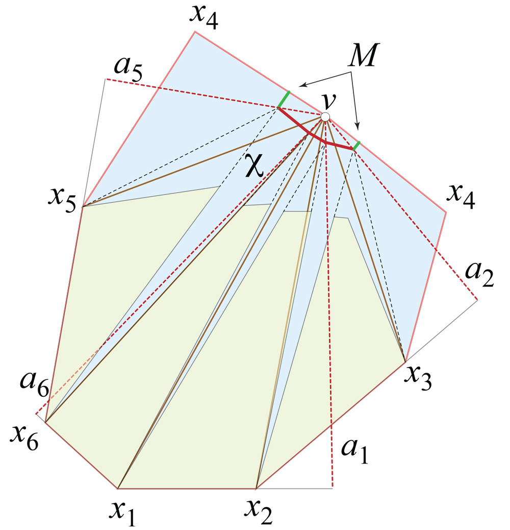
Figure 7.7: The layout from Fig. 7.2(c) shown with moat $M$ and altitudes $a_{i}$ marked. Note $a_{3}$ and $a_{4}$ are missing because $T_{3}$ and $T_{4}$ are clipped as outside $X$. The green edges mark the closing of the partial moat around $v$.

This renders Lemma 7.3 true for the lifted triangles along the convex chain of $\partial L$, which are the only ones not clipped entirely away. We summarize in a theorem:

Theorem 7.4.

A crest $\chi$ can be constructed as the portion of $L$ not covered by lifted triangles in the case of $\bar{v}\in X$, and clipped lifted triangles in the case $\bar{v}\not\in X$, as described above.

We remark that the same procedure will work for other points $w\in X$ within some neighborhood of $\bar{v}\in X$, resulting in different crests. However, a simple example shows that not every point $w\in X$ will produce a crest. Consider $X=x_{1}x_{2}x_{3}$ an equilateral triangle of center $o$, and $v$ close to $o$, with $vo$ orthogonal to $X$. Take $w\in ox_{3}$ close to $x_{3}$. Then the isosceles triangle $wx_{1}x_{2}$ is larger than the isosceles triangle $vx_{1}x_{2}$, so no congruent copy of the former can fit inside $L$ without encompassing $v$ and so self-overlapping.

We have this as a counterpart to Theorem 4.6:

Theorem 7.5.

For any convex polyhedra $P$ and $Q$, one can crest-tailor $P$ to any homothetic copy of $Q$ inside $P$, in time $O(n^{4})$, where $n=\max\{|P|,|Q|\}$.

Proof.

The lemmas leading to Theorem 4.6 established that ultimately we need to tailor single vertex truncations, i.e., tailor pyramids. So the claim follows from Theorem 7.4. ∎

7.3 Algorithm 4: pyramid $\to$ crest

Input : A pyramid $P=L\cup X$ of $O(n)$ vertices

Output : Crest $\chi$ whose removal flattens $P$ to $X$.

// Assume apex $v$ degree-$k$, with $k=O(n)$.

// See Figs. 7.1 and 7.2.

for each of $\bar{T}_{i}$, $i=1,2,\ldots,k$ do

      

      Compute where $\bar{T}_{i}$ edges (geodesics) cross $x_{j}v$. // $O(n)$.

      

      Clip $\bar{T}_{i}$ to $X$. // $O(n)$.

      

end for

Result: Crest $\chi$.

Algorithm 4 Construct a crest $\chi$ that reduces a pyramid $P$.

The total cost of computing one crest $\chi$ is $O(n^{2})$, and we believe there are examples with total combinatorial complexity (number of geodesic/edge intersections) of $\Omega(n^{2})$. Because this is the same complexity for reducing $P$ to $X$ via digon-tailoring described in Chapter 6, the total time complexity is the same as in Theorem 6.2.

We are assuming that the combinatorial complexity of the crest $\chi$ on $L$ determines the time complexity of computing the crest. However, a crest flattened to the plane, not overlaid on $\bar{L}$, has combinatorial complexity $O(n)$—just $k=O(n)$ (possibly clipped) triangles—and can be constructed in $O(n)$ time. Perhaps an implicit representation of shortest paths could suffice for subsequent calculations, as they do in the optimal algorithm for shortest paths on a convex polyhedron [SS08]. Thus it may be that constructing an implicit representation of $\chi$ could lead to a lower time-complexity, a question we leave for future work.

Chapter 8 Tailoring via Flattening

In this chapter, we prove a completely different method for tailoring $P$ to $Q$. The method mixes digon-tailoring steps with vertex-merge steps (Section 2.4). The result is slightly weaker than either tailoring via sculpting (Theorem 4.6) or crest tailoring (Theorem 7.5), weaker in the sense that the homothet of $Q$ obtained could be arbitrarily small. Nevertheless, the proof and algorithm have the advantage of operating entirely intrinsically: the 3D structure of $P$ and $Q$ is never invoked.

The proof depends on the observation that if both $P$ and $Q$ are doubly-covered polygons, it is easy to tailor one to the other: Scale $Q$ to fit in $P$, and then cut the outline of $Q$ from $P$. This can be accomplished by a series of digon-tailorings, with each digon bounded by congruent segments on both sides, or by truncations of several vertices at once.

At a high level, $Q$ is reduced to a flat polygon $Q_{\textrm{flat}}$, $P$ is reduced to a flat polygon $P_{\textrm{flat}}$ and tailored to match $Q_{\textrm{flat}}$. Finally, the steps used to reduce $Q$ are reversed and applied to the flat remnant of $P$.

In more detail, the proof (and algorithm that follows the proof) can be summarized in these steps:

1. Reduce $P$ to $P_{\textrm{flat}}$ by a series of digon tailorings.

2. Reduce $Q$ to $Q_{\textrm{flat}}$ by a series of vertex-mergings. $Q_{\textrm{flat}}$ is then composed of all of $Q$’s surface, plus surface-inserts from the merges.

3. Scale $Q_{\textrm{flat}}$ to $Q^{s}_{\textrm{flat}}$ so that $Q^{s}_{\textrm{flat}}$ fits inside $P_{\textrm{flat}}$.

4. Trim $P_{\textrm{flat}}$ to match $Q^{s}_{\textrm{flat}}$ via digon-tailoring. Call the result $P^{s}_{\textrm{flat}}$.

5. Reverse the vertex-merging steps that reduced $Q$ to $Q_{\textrm{flat}}$, but now applied to $P^{s}_{\textrm{flat}}$. Each reversal step removes a surface-insert via digon-tailoring.

The end result, call it $Q^{t}$, is a polyhedron homothetic to $Q$, but composed entirely of $P$-surface.

We now prove these steps, tracking an example that reduces a cube $P$ to the $5$-vertex polyhedron $Q$ in Fig. 2.6(a), repeated in Fig. 8.2(a).

8.1 Proofs

We follow the numbered outline above.

8.1.1 Digon-tailor $P\to P_{\textrm{flat}}$

Recall that Lemma 2.2 showed that, if the cut locus $C(x)$ is a path, then the polyhedron is a doubly-covered convex polygon. We use this lemma to reduce $P$ to $P_{\textrm{flat}}$.

We will use the cube example from Fig. 2.2 to illustrate the steps. Assume $P$ is non-degenerate, i.e., not flat. Let $x\in P$ be a point joined by unique geodesic segments to all vertices of $P$, and let $\rho$ be the unique path in $C(x)$ joining a pair of leaves of $C(x)$, i.e., joining the vertices $v_{i}$ and $v_{j}$ of $P$.

Then $C(x)\setminus\rho$ is a finite set of trees $T_{k}$. Cut off from $P$ each $T_{k}$ by excising digons with one endpoint at $x$, and the other endpoint where $T_{k}$ joins $\rho$. In Fig. 8.1(a), $\rho$ connects $v_{5}$ and $v_{7}$, and separates four trees $T_{i}$. After sealing each digon closed, we are left with a polyhedron $P_{\textrm{flat}}$ whose cut locus from the point corresponding to $x$ is precisely $\rho$ (by Lemma 2.2).

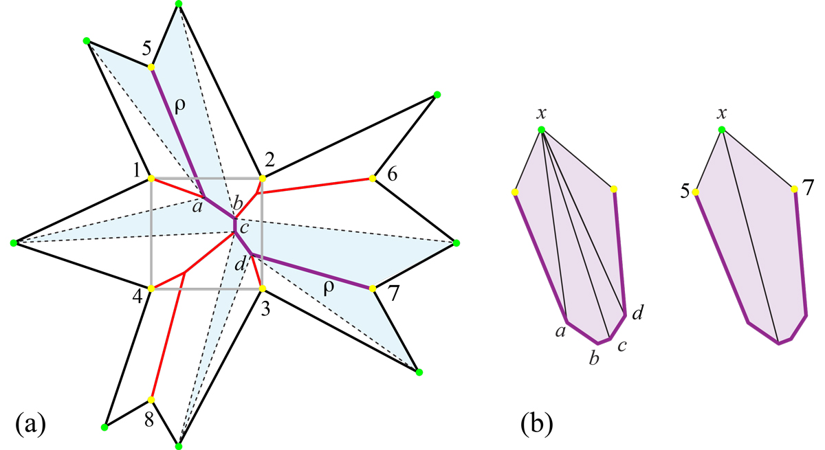
Figure 8.1: Star unfolding of the cube in Fig. 2.2. (a) The path $\rho$ from $v_{5}$ to $v_{7}$ leaves four trees when removed from $C(x)$. Excising four (white) digons leaves a surface (blue), which when zipped closed folds to a doubly-covered $7$-gon, both sides of which are shown in (b).

If the path $\rho$ in the above proof is chosen to be as long as possible, then $P_{\textrm{flat}}$ has larger surface area than if $\rho$ is short.

8.1.2 Vertex-merge $Q\to Q_{\textrm{flat}}$

Recall from Section 2.4 that vertex-merging is in a sense the inverse of digon-tailoring. Two vertices are merged along a geodesic ${\gamma}$ and additional surface in the form of two congruent triangles is sutured-in along ${\gamma}$. Lemma 2.11 showed that every convex polyhedron $Q$ has at least one pair of vertices that can be merged, unless $Q$ is an isosceles tetrahedron or a doubly-covered triangle. So repeatedly vertex-merge $Q$ until it becomes flat, or is reduced to an isosceles tetrahedron.

In our example, Fig. 8.2(a) shows $Q$, the same polyhedron in Fig. 2.6(a). The first vertex-merge leads to a regular tetrahedron, (c) in the figure. As we discussed in Example 1.3 and illustrated in Fig. 1.4, an isosceles tetrahedron can be reduced to a doubly-covered rectangle by cutting an edge and regluing that edge differently. Here we cut the edge $cd$ of the tetrahedron and reglue it by creasing at the midpoints $y_{1},y_{2}$ of the $cd$ slit, leading to the rectangle shown in (d).

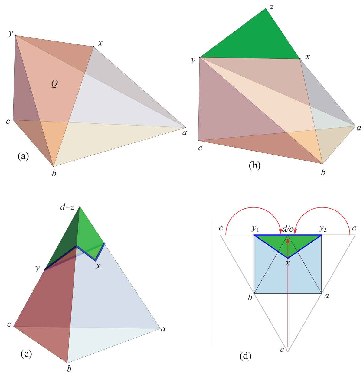
Figure 8.2: (a,b) Vertex-merge of $xy$. (Repeat of Fig. 2.6.) Green indicates surface-inserts. (c) After first vertex-merge. (d) After second special-case vertex-merge: doubly-covered square. (Images not to same scale.)

8.1.3 Scale $Q_{\textrm{flat}}\to Q^{s}_{\textrm{flat}}$

The flattening of $P$ has reduced it in size in the sense that a portion of $P$’s surface area has been excised, while the flattening of $Q$ has augmented it by surface insertions and so has increased $Q$’s surface area. We next select a scale factor $s>0$ so that $Q^{s}_{\textrm{flat}}$ can fit inside $P_{\textrm{flat}}$. Clearly this is always possible. In our example, the scaling might result in Fig. 8.3(a). Note that we should view the top side of $Q^{s}_{\textrm{flat}}$ on the top side of $P_{\textrm{flat}}$, and similarly for the bottom sides.

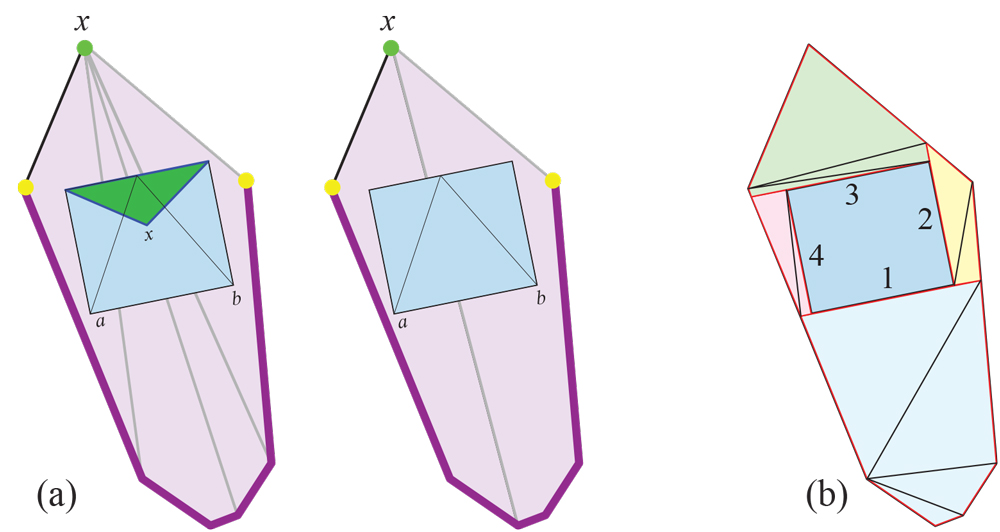
Figure 8.3: (a) $Q$ scaled to $Q^{s}_{\textrm{flat}}$ to fit in $P_{\textrm{flat}}$. (b) Trimming digon excisions by extending the edges of $P_{\textrm{flat}}$ in the order indicated.

8.1.4 Trim $P_{\textrm{flat}}\to P^{s}_{\textrm{flat}}$

As mentioned earlier, it is easy to tailor a doubly-covered convex polygon $P_{\textrm{flat}}$ to match a doubly-covered polygon $Q^{s}_{\textrm{flat}}$ that fits inside $P_{\textrm{flat}}$. This is in some sense similar to sculpting $P_{\textrm{flat}}\to P^{s}_{\textrm{flat}}$. The differences are that (1) here we only work in two dimensions, and (2) this 2D sculpting is an intrinsic operation as well. Fig. 8.3(b) shows one possible sequence of digon tailorings for our example. We extend edge $e$ of $P^{s}_{\textrm{flat}}$ to a line $l_{e}$ which intersects $P_{\textrm{flat}}$, thus separating out a doubly-covered convex polygon, and repeat this for all edges $e$. Then each of those convex polygons is tailored one vertex at a time, say tracking a triangulation.

8.1.5 Reverse $P^{s}_{\textrm{flat}}\to Q^{t}$

Finally we reverse the vertex-merge steps that produced $Q_{\textrm{flat}}$, but applied to $P^{s}_{\textrm{flat}}$. In our example, the last vertex-merge was the special-case step that produced the rectangle in Fig. 8.2(d). The reverse step cuts the top edge $y_{1}y_{2}$ between the two images of $y$, and re-joins $y_{1}$ to $y_{2}$, leading to the regular tetrahedron in (c) of the figure. Reversing the first vertex-merge applied to $Q$ excises the inserted surface, green in (c), resulting in $Q^{t}$, a polyhedron homothetic to $Q$ (Fig. 8.2(a) and 2.6) but composed entirely of $P$-surface.

8.1.6 Theorem: Tailoring via Flattening

We have established this theorem:

Theorem 8.1.

For any given convex polyhedra $P$ and $Q$, one can tailor $P$ “via flattening” so that it becomes homothetic to $Q$.

Remark 8.2.

The result $Q^{t}$ obtained by Theorem 8.1 may be arbitrarily small compared to $Q$.

1. The example of a regular pyramid shows that the area of $P_{\textrm{flat}}$ may be as small as $2/n$ of the original area of $P$.

2. The ratio between the area of $Q_{\textrm{flat}}$ and the area of $Q$ can be arbitrarily large.

   See Fig. 8.4.

   

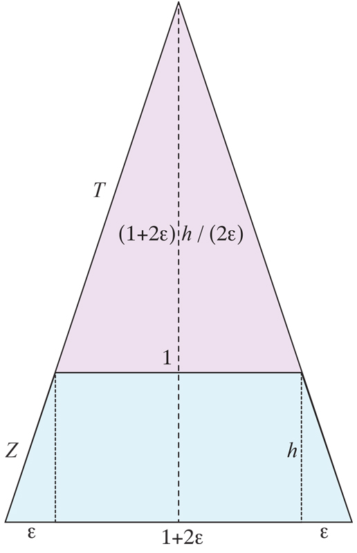
   Figure 8.4: The ratio of the areas of $T$ and $Z$ is arbitrarily large.

   To see this, consider an isosceles trapezoid $Z$ of base lengths $1$ and $1+2\varepsilon$, and height $h$. Its area is $(1+\varepsilon)h$. Also consider the isosceles triangle $T$ obtained from $Z$ by extending its non-parallel sides until intersecting. An elementary geometry argument provides the height of $T$, $(1+2\varepsilon)h(2\varepsilon)^{-1}$, and the area of $T$, $(1+2\varepsilon)^{2}h(4\varepsilon)^{-1}$.

   The ratio between the area of the doubles $Q_{\textrm{flat}}$ of $T$, and $Q$ of $Z$, is therefore

   $$\frac{(1+2\varepsilon)^{2}}{4\varepsilon(1+\varepsilon)}=1+\frac{1}{4\varepsilon(1+\varepsilon)}$$

   and can be arbitrarily large for $\varepsilon$ arbitrarily small.

The combination of $P_{\textrm{flat}}$ small and $Q_{\textrm{flat}}$ large leads to the arbitrarily-small claim for $Q^{t}$ with respect to $Q$.

8.2 Algorithm for Tailoring via Flattening

Input : Convex polyhedra $P$ and target $Q$

Output : A tailored version of $P$ homothetic to $Q$

// (1) Reduce $P$ to $P_{\textrm{flat}}$.

Find generic point $x$. // $O(n^{4})$

Compute cut locus $C(x)$. Select path $\rho$. Digon removals of trees until $P_{\textrm{flat}}$ attained.

// (2) Vertex merge on $Q$ repeatedly.

while $Q\neq T_{\textrm{isos}}$ and $|Q|>3$ do

      

      Identify two vertices $v_{i}$ and $v_{j}$ such that ${\omega}_{i}+{\omega}_{j}<2\pi$. // $O(n^{2})$

      

      Vertex merge $v_{i}$ and $v_{j}$, reducing $Q$ by one vertex to $Q^{\prime}$.

      $Q\leftarrow Q^{\prime}$.

end while

if $Q=T_{\textrm{isos}}$ then // $Q$ isosceles tetrahedron

       Special tailor $Q$ to flat rectangle $Q_{\textrm{flat}}$.

end if

// (3) Scale $Q_{\textrm{flat}}$ to $Q^{s}_{\textrm{flat}}$.

Find largest inscribed and smallest circumscribed circles. // $O(n)$.

Scale $Q_{\textrm{flat}}$ by radii ratio.

// (4) Trim $P_{\textrm{flat}}$ to $P^{s}_{\textrm{flat}}$.

Extend edges of $P^{s}_{\textrm{flat}}$, triangulate each cut-off piece. // $O(n^{2})$.

// (5) Reverse steps to reduce $Q$, each applied to $P^{s}_{\textrm{flat}}$

foreach vertex-merging step applied to $Q$ do

      Reverse the step by cutting off the merge vertex.

end foreach

Result: A 3D polyhedron $Q^{t}$ homothetic to $Q$.

Algorithm 5 Tailor $P$ to $Q$ via Flattening.

In this section, we follow the proof of Theorem 8.1 and convert it to a polynomial-time algorithm.

As usual, let $n=\max\{|P|,|Q|\}$ be the combinatorial size of the polyhedra. We now establish an upper bound of $O(n^{4})$ on the complexity of implementing the algorithm.

Step (1) is to tailor $P$ to $P_{\textrm{flat}}$ using the cut locus $C(x)$ from a “generic point” $x$, i.e., one with a unique shortest path to each vertex of $P$. Although it is possible the need for uniqueness could be avoided, we leave that future work. We know of no way to find a generic $x$ short of computing all the “ridge-free” regions on $P$, which takes $O(n^{4})$ time [AAOS97]. Independent of our work here, it is a interesting question if a generic $x$ can be computed more quickly. We will see this $O(n^{4})$ dominates the complexity of the other calculations.

The star-unfolding $S_{P}(x)$ can be computed in $O(n\log n)$ time using the complex Schreiber-Sharir algorithm [SS08], or in $O(n^{2})$ time with the Chen-Han algorithm [CH90, CH96]. $S_{P}(x)$ only needs to be computed once. With $S_{P}(x)$ computed, the cut locus $C(x)$ can be found from the Voronoi diagram of the images of $x$.

Step (2) is to repeatedly apply vertex-merging to $Q$ until it is reduced to $Q_{\textrm{flat}}$, when $|Q_{\textrm{flat}}|\in\{3,4\}$. Identifying two vertices $v_{i}$ and $v_{j}$ such that ${\omega}_{i}+{\omega}_{j}<2\pi$ can be achieved in $O(n\log n)$ time just by sorting the curvatures ${\omega}_{i}$ and selecting the two smallest. From the initial sorting onward, only $O(\log n)$ would be needed to update the list, but we’ll see this efficiency is not necessary.

With $v_{i}$ and $v_{j}$ selected, the shortest path ${\gamma}$ between them needs to be computed. Although there is a complicated optimal $O(n\log n)$ algorithm for computing shortest paths on a convex polyhedron [SS08], that algorithm exploits the three-dimensional structure of the polyhedron, which will not be available to us after the first vertex-merge. As mentioned earlier, there is no effective procedure known to construct the polyhedron guaranteed by AGT. However, we know the intrinsic structure of the polyhedron: its vertices, their curvatures, a triangulation. The algorithm of Chen and Han [CH90, CH96] can compute shortest paths from this intrinsic data in $O(n^{2})$ time. Repeating this $n$ times to reach $Q_{\textrm{flat}}$ then can be achieved in $O(n^{3})$ time.

The scaling step (3) can be accomplished in linear time, $O(n)$, as follows. The largest circle inscribed in $P_{\textrm{flat}}$ is computed by the linear-time medial axis algorithm [CSW99]; say its radius is $r_{P}$. The smallest circle circumscribing $Q_{\textrm{flat}}$ is found in linear-time via Megiddo’s algorithm [Meg83]; say its radius is $r_{Q}$. Then scale $Q_{\textrm{flat}}$ by $s=r_{P}/r_{Q}$.

Trimming $P_{\textrm{flat}}$ to $P^{s}_{\textrm{flat}}$, step (4), can be accomplished in many ways. The method we described in Section 8.1.4 can easily be implemented in $O(n^{2})$ time by ray-shooting the edge extensions, and then triangulating each convex polygon in linear time. Likely the ray-shooting could be reduced to $O(n\log n)$ time.

Reversing the $Q$ vertex-merging steps, step (5), amounts to digon tailorings cutting of the merged vertices on $P$. This can easily be accomplished in $O(n\log n)$ time. Keeping track of the considered vertices and employed digons gives in the end a correspondence between $Q^{t}$ and $Q$, and thus the 3D structure of $Q^{t}$.

So the whole algorithm time-complexity is dominated by the $O(n^{4})$ cost of finding a guaranteed generic $x$.

Because the ridge-free regions are determined by overlaying $n$ cut loci, the regions are delimited by a one-dimensional network of segments. Thus choosing a random point $x$ on $P$ is generic with probability $1$. That still leaves the algorithm requiring $O(n^{3})$ time. We believe this time complexity could be improved, perhaps to $O(n^{2})$. See Open Problem 18.1.

We repeat Theorem 8.1 with the complexity bound included:

Theorem 8.3.

For any given convex polyhedra $P$ and $Q$, one can tailor $P$ until it becomes homothetic to $Q$ in time $O(n^{4})$, where $n=\max\{|P|,|Q|\}$.

Finally, we note that our model of reshaping in all cases excises just a single vertex via a tailoring step, or inserts a single vertex via a vertex-merge step. A rather different model, but related to the flattening algorithm above, unfolds $P$ and $Q$ each to nets (non-overlapping planar polygons), and places the unfolded $Q$ inside the unfolded $P$. For example, Jin-ichi Itoh made the following interesting suggestion: first star-unfold $P$ to $S_{P}$ and $Q$ to $S_{Q}$, shrink $S_{Q}$ to fit inside $S_{P}$, then cut out $S_{Q}$ from $S_{P}$, and refold to obtain a homothet of $Q$ from $P$.

Chapter 9 Enlarging, $P$-Unfoldings, and Continuous Foldings

In this chapter we show how to enlarge a convex polyhedron $Q$ to some $P\supset Q$, via tailoring. Based on this operation, we introduce the notion of a $P$-unfolding and propose a few methods to accomplish it. Finally, we describe a method to continuously fold $P$ onto an enclosed $Q$.

9.1 Enlarging and Reshaping

Previous chapters have established three methods of tailoring $P$ to $Q$:

• Theorem 4.6: For $Q\subset P$, digon-tailor following a sculpting of $P$ to $Q$.

• Theorem 7.5: For $Q\subset P$, crest-tailor following a sculpting of $P$ to $Q$.

• Theorem 8.1: via flattening, digon-tailor $P$ to a (possibly small) homothet of $Q$.

If we do not have $Q\subset P$, then shrinking $Q$ until it can fit in $P$ leads to a homothet of $Q$. All three approaches result in the homothet of $Q$ being composed entirely of $P$-surface. In the tailoring-via-flattening algorithm, $Q$ is enlarged with vertex-merging inserts, but the last steps remove all inserts.

In this short chapter, we explore some results that can be achieved through a mix of vertex-merge enlarging, and tailoring. Part II will explore vertex-merging more thoroughly.

Suppose $Q\subset P$. Then we can enlarge $Q$ to $P$ using any one of the three tailoring algorithms, as follows. We first tailor $P$ to $Q$, tracking the cuts and digons removed. For crest-tailoring, we cut the boundary of crests. Then, starting with $Q$, we cut each sealed geodesic or crest-boundary and insert the earlier removed corresponding digon or crest surface, in reverse order. The result is that $Q$ is enlarged by the surface insertions (of $P$-surface) in the reversing process until it matches $P$.

If $Q\not\subset P$, so $P$ and $Q$ are of arbitrary relative sizes, we can reshape $P$ to $Q$ by first enlarging $P$ to some $P^{\prime}\supset Q$ large enough to enclose $Q$, and then tailor $P^{\prime}$ to $Q$. Here $P^{\prime}$ is an arbitrary polyhedron midway in the process $P\to P^{\prime}\to Q$; it only needs to be large enough.

These enlargings can be accomplished within the same $O(n^{4})$ time complexity of the tailoring algorithms. And in analogy with Corollary 4.7, enlargings of $Q$ can approximate any target surface $S$.

We summarize the above discussion in a theorem:

Theorem 9.1.

Let $P$ and $Q$ be convex polyhedra. If $Q\subset P$, $Q$ may be enlarged with surface insertions to $P$. If $Q\not\subset P$, $P$ can be reshaped to $Q$ with a combination of surface insertions and excisions. Either process can be accomplished in time $O(n^{4})$, and can approximate non-polyhedral convex surfaces.

9.2 $P$-unfoldings

For $Q\subset P$, we can view the enlarging of $Q$ to $P$ just described as “unfolding” $Q$ onto $P$. We call this a $P$-unfolding of $Q$. To our knowledge, this notion has not been considered previously. We explore it briefly here, and in more detail in Part II.

9.2.1 $P$-unfoldings and Reshaping

Unfoldings of convex polyhedra to a plane have been studied extensively; see, e.g., [DO07]. Particular attention has been paid to unfolding to few pieces, to connected unfoldings, and to non-overlapping unfoldings. Often the goal is to achieve a net, an unfolding to a single, simply connected, non-overlapping polygon in the plane.

Instead of unfolding a convex polyhedron $Q\subset P$ to a plane, consider the question: Can one cut-up the surface $Q$ so that the pieces may be pasted onto $P$, non-overlapping, and so form an isometric subset of $P$? This is a $P$-unfolding of $Q$, or an unfolding of $Q$ onto $P$. It can be achieved via enlarging: just enlarge $Q$ to $P$, and then remove all inserted digons or crests. The result is a subset of $P$ isometric to the cut-up $Q$. Note that all three enlarging methods retain the entire surface of $Q$—the enlarging is accomplished by insertions of surface not part of $Q$.

This viewpoint incidentally yields a different proof of this known result:

Corollary 9.2.

Given convex polyhedra $P$ and $Q\subset P$, the area of $Q$ is smaller than the area of $P$.

To justify the use of the term “unfolding,” we describe an example of a simply connected $P$-unfolding embedding that does not achieve a net when unfolded to a plane. Let $Q$ be the classical thin, nearly flat tetrahedron with an overlapping edge-unfolding. See, e.g., [DO07, Fig. 22.8, p. 314]. Take $P$ to be a slightly larger homothet of $Q$. Then the same edge-cuts that result in overlap in the plane embed $Q$ onto $P$ without overlap. In a sense, it can be easier in some cases to unfold to $P$ than to unfold to a plane.

One focus of interest in the unfolding literature is the “fewest nets” problem [DO07, Prob. 22.1, p. 308]: edge-unfold a polyhedron into the fewest number of nets. Of course one net would be ideal, but it is a long-standing open problem to determine if every convex polyhedron can be edge-unfolded to a net—Dürer’s problem [O’R13]. This suggests it could be of interest to minimize the number of disconnected pieces of a $P$-unfolding of $Q$, a goal we pursue in Part II. See also Open Problem 18.4.

Example: Hexagon inscribed in a triangle.

Let $P$ be a doubly-covered triangle $abc$, and $Q$ a doubly-covered hexagon inscribed in $P$, as in Fig. 9.2. Digon-tailoring $P$ to $Q$ is achieved by excising the vertices $a,b,c$ by cutting digons bounded by the hexagon edges $e_{1},e_{2},e_{3}$ respectively, and then sealing the cuts closed. To enlarge $Q$ to $P$ by reversing the process, each of those three edges is slit open and the pair of triangles earlier removed is sutured back along the slit edges. To obtain a $P$-unfolding, we simply skip inserting the pair of triangles. The result is a “pasting” of the two hexagons inside the two triangular faces of $P$.

Note that, to reverse a sealed digon, the resulting geodesic ${\gamma}$ is slit, but the cut does not delete the endpoints $x_{1},x_{2}$ of ${\gamma}$, as depicted in Fig. 9.2. In other words, ${\gamma}\setminus\{x_{1},x_{2}\}$ is doubled to reproduce the digon boundary, but there remains one copy each of the $x_{1},x_{2}$ endpoints.

Notice that each split $e_{i}$ is —bluea non-contractible closed curve inside the image of $Q$, so the embedding of $Q$ onto $P$ in this case is not simply connected: it has three holes.

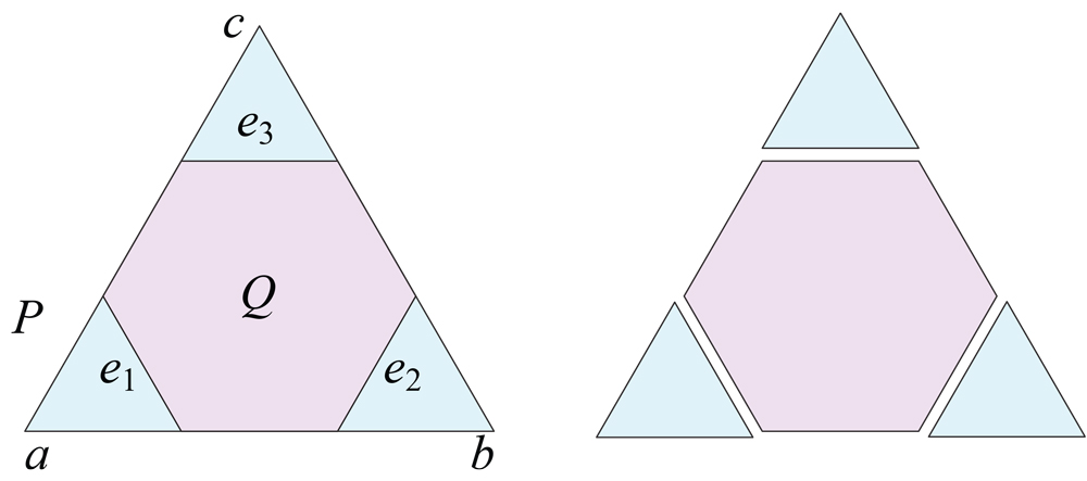
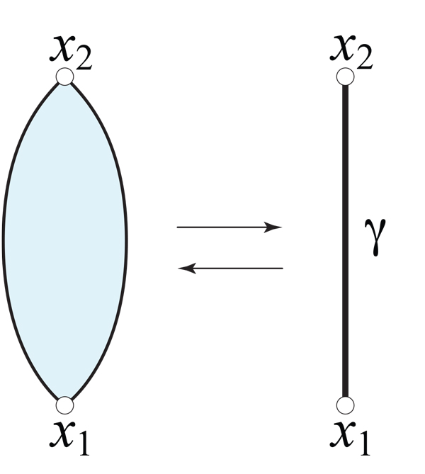
Figure 9.1: Doubly-covered hexagon $Q$ inscribed inside / enlarged to a doubly-covered triangle $P$.

Figure 9.2: Digon $x_{1}x_{2}$ closes to geodesic ${\gamma}$.

The previous example shows that the $P$-unfolding of $Q$ produced by enlarging is not necessarily simply connected. However, in general, that is indeed the case, as shown by the following result. We next explain the meaning of “in general.”

Consider the space ${\cal S}$ of all convex surfaces, endowed with the topology induced by the usual Pompeiu-Hausdorff metric. Fix some $P\in{\cal S}$. Consider in ${\cal S}$ the subset ${\cal P}={\cal P}_{P}^{n}$ of all polyhedra $Q\subset P$ with precisely $n$ vertices, with the induced topology. Two polyhedra in ${\cal P}$ are then close to each other if and only if they have close corresponding vertices. “General” refers to polyhedra $Q$ in an open and dense subset of ${\cal P}$.

Theorem 9.3.

For any convex polyhedron $P$ and any $n\in{\mathbb{N}}$, there exists a subset ${\cal Q}={\cal Q}_{P}^{n}$ open and dense in ${\cal P}$, such that the $P$-unfolding $Q_{P}$ of each $Q\in{\cal Q}$ is flat (i.e., contains no internal vertices), and is simply connected.

Proof.

Assume we have some convex polyhedron $Q\subset P$ such that $Q_{P}$ contains an internal vertex $v$, and so the curvatures of $P$ and $Q$ at $v$ are equal: ${\omega}_{Q}(v)={\omega}_{P}(v)$. Slightly alter the position of the vertices of $Q$, to get ${\omega}_{Q}(w)\neq{\omega}_{P}(u)$, for any vertices $w\in Q$ and $u\in P$. Of course, this remains valid in a small neighborhood of the new $Q$.

Assume now we have some convex polyhedron $Q\subset P$ such that $Q_{P}$ is not simply connected, i.e., $Q_{P}$ contains a noncontractible curve ${\sigma}\subset P\cap Q_{P}$. The Gauss-Bonnet Theorem shows that the total curvature $\Omega_{Q}({\sigma})$ of $Q_{P}$ inside ${\sigma}$ equals the total curvature $\Omega_{P}({\sigma})$ of $P$ inside ${\sigma}$: $\Omega_{Q}({\sigma})=\Omega_{P}({\sigma})$. We next show that every such $Q$ that violates the theorem can be approximated with polyhedra that do satisfy the theorem.

Slightly alter the position of the vertices of $Q$, to get a new polyhedron $Q^{\prime}$ on which the following property (V) is verified. (V): any partial sum of vertex curvatures is different from any partial sum of vertex curvatures in $P$. This implies that, for any simple closed curve ${\tau}$ on $Q^{\prime}$, $\Omega_{Q^{\prime}}({\tau})$ cannot be written as the sum of vertex curvatures of $P$. Therefore, $Q^{\prime}_{P}$ has no curve in common with $P$, noncontractible in $Q^{\prime}_{P}$. And so $Q^{\prime}$ does satisfy the theorem.

Since the property (V) is valid on a neighborhood $N$ of $Q^{\prime}$, it follows that all polyhedra in $N$ do satisfy the theorem. ∎

9.2.2 $P$-unfoldings and the WBG Theorem

In this section we show that the $P$-unfolding question can also be answered by applying the powerful hinged variant of Wallace-Bolyai-Gerwien dissection theorem. However, this will result in a “pseudopolynomial number of pieces” and pseudopolynomial running time [AAC⁺12].

The Wallace-Bolyai-Gerwien (WBG) Theorem states that any two simple polygons with equal area can be dissected into finitely many simple congruent polygons. It was strengthened in the paper, “Hinged Dissections Exist” [AAC⁺12], where it is shown that the pieces can be chosen in an arcwise-connected chain, i.e., the dissection can be hinged at vertices along that chain.

Theorem 9.4.

Given convex polyhedra $P$ and $Q$ of at most $n$ vertices each, and $Q\subset P$, a connected $P$-unfolding of $Q$ can be determined in pseudopolynomial number of pieces and pseudopolynomial running time, following the WBG theorem and the hinge-dissection.

Proof.

We start with a quote from [AAC⁺12]:

“One interesting consequence of [our] theorem is that any finite set of polyhedral surfaces of equal surface area have a common hinged dissection: It is known that every polyhedral surface can be triangulated and then vertex-unfolded into a hinged chain of triangles [DEE⁺03]. Our results (specifically Theorem 6) show how to construct a single hinged chain that can fold into any finite set of such chains, which can then be folded (and glued) into the polyhedral surfaces.”

A vertex-unfolding of a triangulated polyhedron is a chain of triangle connected at vertices. A vertex-unfolding of a triangulated cube is shown in Fig. 9.3.

Let $A_{Q}$ and $A_{P}$ be the areas of $Q$ and $P$. Triangulate and vertex-unfold both $P$ and $Q$. The plan is to show that $A_{Q}$ can “fit” exactly within a sequence of $P$’s triangles, with at most one of $P$’s triangles partitioned into two triangles.

Denote by $T_{1},...,T_{m}$ the triangles in the chain corresponding to $P$, and by $a_{j}$ denote the area of the $T_{j}$, $j=1,...,m$. So we have $A_{Q}<A_{P}=\sum_{j=1}^{m}a_{j}$. Then there exists $1\leq h\leq m$ such that $a_{1}+...+a_{h-1}\leq A_{Q}<a_{1}+...+a_{h}$. Triangle $T_{h}$ is then the transitional triangle with respect to area in the sequence of triangles.

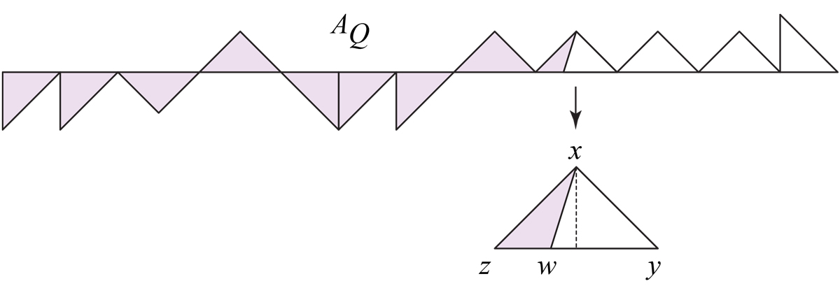
Figure 9.3: Area $A_{Q}$ (shaded) in vertex-unfolding of a triangulated cube. $T_{h}=xyz$. Based on Fig.2(a) in [DEE⁺03].

Now we further dissect the triangle $T_{h}$ into two parts, one of which has area $c=A_{Q}-(a_{1}+...+a_{h-1})$. Specifically, let $T_{h}=xyz$ and choose a point $w\in yz$ such that $|w-y|/|z-y|=c/a_{h}$. Then the area $A^{\prime}$ of the triangle $xyw$ is equal to $c/a_{h}$ of the area of $T_{h}$ (because both triangles have the same altitude through $x$).

Therefore, in the chain of triangles obtained from $P$, we can find an arcwise-connected subchain of total area equal to $A_{Q}$, possibly after partitioning one triangle.

Then Theorem 6 in [AAC⁺12] constructs a single hinged dissection chain of the triangles forming $Q$ into the triangles up to $T_{h}$ of $P$. Then the $Q$-chain triangles can be placed inside the $P$-chain triangles, achieving a connected $P$-unfolding of $Q$.

The “pseudopolynomial number of pieces” and pseudopolynomial running time follows from [AAC⁺12]. ∎

Note that although the $P$-unfolding constructed in this theorem’s proof is connected, its interior is not connected.

9.3 $P$ Continuously Folding onto $Q$

Cauchy’s Rigidity Theorem shows that if one views the faces of a convex polyhedron as rigid plates hinged along shared edges, then the polyhedron is rigid—it cannot flex. For both convex and nonconvex polyhedra, a line of research has explored continuous flattening of a polyhedron to a plane [DO07, Chap.18]. The idea is to allow “moving” or “rolling” creases, allowing the faces of the polyhedron to bend, but not tear or pass through one another. An early result was a method to flatten each of the five Platonic solids [IN10]. This was followed by procedures for continuously flattening all convex polyhedra [INV12], [ADD⁺14]. Most recently, continuous flattening of any polyhedron was achieved by extending the model to permit infinite slicing [ADD⁺21].

All of these results aim to fold the polyhedron to a “flat folded state”—a non-self-crossing layering of the surface on a plane. Here we employ the tailoring/sculpting result (Theorem 6.2) to address what appears to be a novel variation: continuously folding the surface of one convex polyhedron onto another.

In particular, we follow the slicing algorithm as summarized in Theorem 6.2: Given convex polyhedra $P$ and $Q$ with $Q\subset P$, $P$ can be tailored to $Q$, tracking a sculpting of $Q$ from $P$ as in Theorem 4.6, via a polynomial number of tailoring steps. This leads to the following theorem.

Theorem 9.5.

Given convex polyhedra $P$ and $Q$ with $Q\subset P$, there exists a continuous folding of $P$ onto $Q$, tracking a sculpting of $Q$ from $P$ as in Theorem 4.6.

Note we claim the existence of a continuous folding, but we do not know how to turn it into a finite algorithm to perform the folding; see Open Problem 18.5. Nevertheless, there are distinct steps.

Recall the tailoring-via-sculping algorithm (Theorem 6.2) ultimately identifies a polynomial number of tailoring steps (polynomial in the number of vertices $n$). The folding in Theorem 9.5 follows the same sequence of digon steps as the tailoring algorithm, but handling each digon differently. From now on we concentrate on the tailoring of a single digon.

The high-level idea is as follows. Instead of excising the digon and suturing closed its two sides, we gradually bring together the two digon sides without removing the interior of the digon. This process forms a growing doubly-covered triangle, which is folded onto the surface of $Q$. Once the digon sides have been joined, we imagine the folded triangle as now melded into $Q$’s surface. Subsequent digon processing may refold earlier foldings.

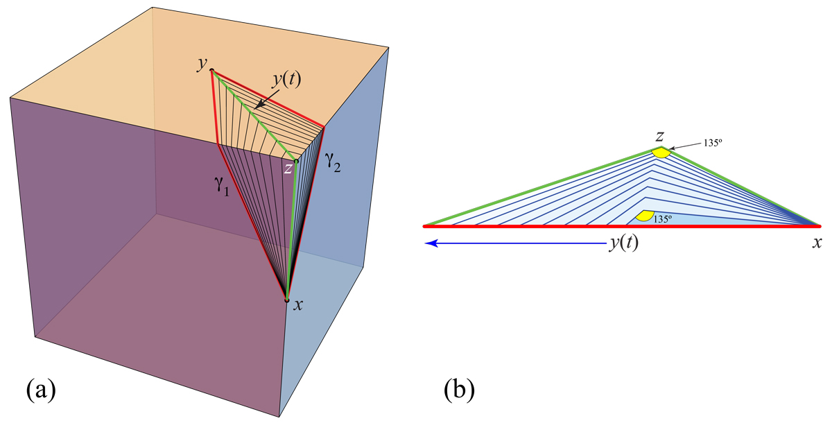
Figure 9.4: (a) Digon $xy$ surrounding vertex $z$. $y(t)$ moves along the geoseg$zy$. (b) Each $t$ leads to a doubly-covered triangle $T(t)$ with apex $z$ and base $xy(t)$. The angle at $z$ is fixed to half of $3\pi/2$ by the curvature of $\pi/2$ at vertex $z$.

Recall from Chapter 1 that a digon $D(x,y)$ is a subset of $P$ bounded by two equal-length geodesic segments ${\gamma}_{1}$ and ${\gamma}_{2}$. The tailoring algorithm only employs digons each surrounding one vertex. If $z$ is the enclosed vertex, then $D(x,y)$ is intrinsically composed of two triangles, one based on ${\gamma}_{1}$ and one of ${\gamma}_{2}$, both apexed at $z$. When ${\gamma}_{1}$ is identified with ${\gamma}_{2}$, then the digon surface forms a doubly-covered triangle $T=xzy$.

In the tailoring algorithm, $D(x,y)$ is excised, ${\gamma}_{1}$ is glued to ${\gamma}_{2}$, and Alexandrov’s Gluing Theorem AGT is invoked to obtain a new convex polyhedron. For continuous folding, we want to gradually close ${\gamma}_{1}$ and ${\gamma}_{2}$ until $T$ is obtained. For this process, we fix $x$ and define a variable $y(t)\in yz$ with boundary conditions $y(0)=z$ and $y(1)=y$. See Fig. 9.4(a). Define ${\gamma}_{1}(t)$ and ${\gamma}_{2}(t)$ to connect the fixed $x$ to the variable point $y(t)$. As $t$ varies from $0$ to $1$, joining ${\gamma}_{1}(t)$ and ${\gamma}_{2}(t)$ lifts a triangle $T(t)=xzy(t)$ outside of the surface of $Q$. We can imagine applying AGT at every infinitesimal advancement of $t\in(0,1]$.

The triangles $T(t)$ each have apex $z$ and a fixed angle at $z$ of $\frac{1}{2}(2\pi-{\omega}(z))$. See Fig. 9.4(b). The base $xy(t)$ of $T(t)$ lengthens with $t$, as does the altitude of $T(t)$. When $t=1$, the digon is closed with ${\gamma}_{1}={\gamma}_{2}$ and $T(1)=T$.

So far we have only observed that $T(t)$ sits outside of $Q$. But at each $t$, we fold $t$ to one side or the other of the geodesic segment $xy(t)$, i.e., ${\gamma}_{1}(t)={\gamma}_{2}(t)={\gamma}(t)$. Because ${\gamma}(t)$ is a geodesic segment, there is a neighborhood $N(t)$ of ${\gamma}(t)$ that is vertex-free, in the sense that it contains no other vertex than $x$ and $y$. See Fig. 9.5(a). If $T(t)$ fits in that neighborhood $N(t)$, then we fold $T(t)$ into $N(t)$ by creasing along ${\gamma}(t)$. Because $N(t)$ is vertex-free, $T(t)$ can flatten into $N(t)$, even if ${\gamma}(t)$ crosses edges of $Q$, because $N(t)$ is isometric to a planar patch of surface, and $T(t)$ is itself planar.

If at some time $t$, $T(t)$ no longer fits into $N(t)$, then we “accordion-fold” the growing $T(t)$ so that it does fit. As the altitude to $z$ grows with $t$, the triangle might need to be folded back and forth, as depicted in Fig. 9.5(b).

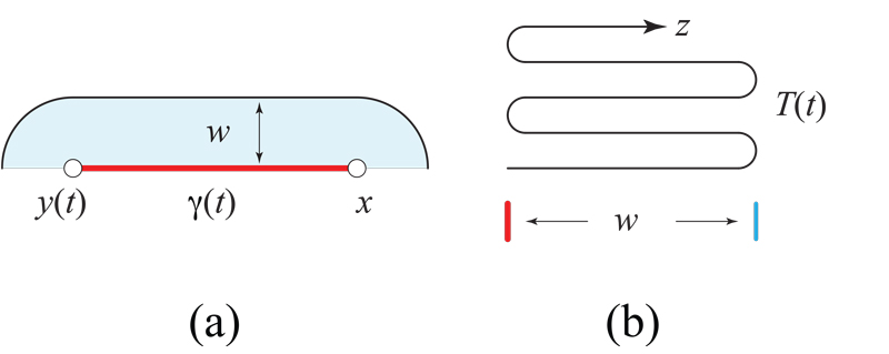
Figure 9.5: (a) Vertex-free region of width $w$ adjacent to geodesic ${\gamma}(t)$. (b) Side view of folding triangle $T(t)$ to fit inside the vertex-free region.

When $t$ reaches $1$, all of $T(1)=T$ is now folded onto $Q$, perhaps in several layers. Now we imagine melding $T$ into $Q$’s surface, and we proceed with the next step of the tailoring algorithm. Note that a subsequent digon, say $x^{\prime}y^{\prime}$, might cross the now closed $xy$ seal. Processing that digon will fold its doubly-covered triangle $T^{\prime}$, intruding underneath and into the earlier triangle $T$. Although the subsequent foldings of $T$ caused by other digons could be quite complicated, we continue to view $T$ as merged with $Q$’s surface, and let the folding of each digon proceed as described, possibly carrying along earlier doubly-covered triangle foldings.

After all digons have been processed in the order specified by the tailoring algorithm, we have successfully continuously folded $P$ onto $Q$, without ever any surface self-crossing.

Part II Vertex Merging and Convexity

Chapter 10 Introduction to Part II

In the second part of our monograph we focus on the operation of vertex-merging on a convex polyhedron $P$. Used before as a proof technique by several authors, starting with A.D. Alexandrov, this operation has never before been considered, to our knowledge, as a main object of study. The operation is defined in Chapter 2, Section 2.4, and we employed it in Part I, in Chapters 8 and 9. We explained in Chapter 8 how vertex-merging is in some sense the inverse of digon-tailoring: instead of cutting off a vertex $v$ by excising a digon, vertex-merging slits a geodesic segment connecting two vertices $v_{1}$ and $v_{2}$, and inserts a pair of triangles that flatten $v_{1}$ and $v_{2}$ and introduce a new vertex $v$ with curvature ${\omega}(v)={\omega}(v_{1})+{\omega}(v_{2})$. One might view this process as “geometric surgery” in analogy with topological surgery, which cuts out part of a manifold and replaces it with part of another manifold, a technique pioneered by John Milnor and further developed by Dennis Sullivan and others.

We called the geodesic segment that results from suturing-closed the digon boundary a seal. We will call the vertex-merge geodesic segment a slit.

A polyhedral surface $S$ that admits no vertex-merging is irreducible. By Lemma 2.11, the irreducible polyhedra are isosceles tetrahedra and doubly-covered triangles.

Vertex-merging reductions—the processes of repeatedly reducing the number of vertices via merging, from $P$ to an irreducible polyhedron—are studied in Chapter 11 together with their induced slit graphs. This can be seen as a theoretical exploration as well as a refinement of a proof idea employed in Chapter 8.

Particularly interesting are the cases when slit graphs are forests of trees, because then the unfolding (i.e., the image) $P_{S}$ of $P$ onto the irreducible surface $S$ has connected interior. Even in this case, obtaining a net from $P_{S}$ is not always obvious, as shown in Section 11.7. The overall goal, and the guiding thread, of this Part II, is to identify slit graphs that are forests of trees.

Our basic algorithmic idea for finding such forests is a certain type of spiraling slit tree. We present this first in the planar limit case in Chapter 12. The analysis is based on planar convex hulls of finitely many points, viewed as vertices of zero curvature. The boundary of such a hull is equivalently obtained as the minimal length enclosing polygon of the given set of points.

Next, we aim to extend to convex polyhedra this idea of spiraling slit trees. Toward this goal, we partition the surface into two half-surfaces, sharing a simple closed quasigeodesic $Q$ as a common boundary. Every convex polyhedron has at least three such quasigeodesics [Pog49][Pog73].

So we are led first to consider, on convex polyhedra, the notions of convexity and convex hull (in Chapter 13) and then the notion of a minimal length enclosing geodesic polygon (in Chapter 14). Although identical in two dimensions, these notions are not equivalent in our framework. As far as we know, they have not been investigated in detail on convex polyhedra. Given their importance in the plane, we believe they have a certain interest in their own right.

In Chapter 15 we show that the extension to half-surfaces (bounded by $Q$) of the planar spiraling algorithm works well for both the convex hull and the minimal length enclosing geodesic polygon, of all vertices inside a simple closed quasigeodesic.

The next step, in Chapter 16, is to join the two slit trees, previously obtained for half-surfaces. Thus we obtain unfoldings of the starting polyhedron $P$ onto the union of two cones, or onto to a cylinder. The last case appears if $Q$ contains at most two vertices, when rolling the cylinder on a plane leads to a net of $P$.

In the penultimate Chapter 17, we prove the existence of a non-empty and open set ${\cal Q}_{\leq 2}$ of convex polyhedra $R$, each polyhedron $R\in{\cal Q}_{\leq 2}$ having a simple closed quasigeodesic with at most two vertices. We also conjecture that such a quasigeodesic exists on all $P$, which would lead to a net of $P$ by rolling.

We end with a list of open problems from both Part I and II in Chapter 18.

Chapter 11 Vertex-Merging Reductions and Slit Graphs

In this chapter we initiate the systematic study of consecutive operations of vertex-merging, already used in Chapter 8. We introduce vertex-merging reductions and their associated slit graphs, and derive their basic properties for later use. Several examples and open problems are discussed. Our main goal, carried out over several chapters and topics, is to relate vertex-mergings to unfoldings and nets. First steps toward this goal are reached in Theorem 11.5 and the discussion that follows in Section 11.6.

11.1 Slit Graphs for Vertex Mergings

Recall from Section 2.4 and the Introduction to Part II that merging of vertices $v_{1}$ and $v_{2}$ is only possible (by Lemma 2.11) when their curvatures ${\omega}_{1},{\omega}_{2}$ satisfy ${\omega}_{1}+{\omega}_{2}<2\pi$. The vertex-merging irreducible surfaces (in short, vm-irreducible) are doubly-covered triangles and isosceles tetrahedra.

A vertex-merging reduction (in short, a vm-reduction) of a convex polyhedron $P$ is a maximal sequence of consecutive vertex-merging steps starting from $P$; maximal, in the sense that it reduces $P$ to a vm-irreducible surface $S$.

Explicitly, during a reduction process we obtain a sequence of convex polyhedral surfaces $P=P_{0},P_{1},\ldots,P_{k}=S$, with $S$ vm-irreducible, and piecewise isometries $\iota_{j}:P_{j}\to P_{j+1}$. Of course, each $\iota_{j}$ is a polyhedral-unfolding of $P_{j}$ onto $P_{j+1}$, as is $\iota=\iota_{k-1}\circ\iota_{k-2}\circ\ldots\iota_{0}:P\to S$, where $\circ$ is the composition of functions. Put $P_{S}=\iota(P)\subset S$.

With some abuse, in the following we shall sometimes consider all isometries above as identities, thus identifying $P_{j}$ and $\iota_{j}(P_{j})\subset P_{j+1}$, for $j=0,\ldots,k-1$.

The slit graph for a vertex-merging reduction $\iota=\iota:P\to S$ is the trace on $P$ of all geodesic segments used during the reduction, called slits. Explicitly, at each reduction step we use a geodesic segment ${\gamma}_{j}$ on $P_{j}$ along which we merge two vertices of $P_{j}$. Notice that $\bar{\iota}_{j}=\iota_{j-1}\circ\ldots\circ\iota_{0}:P\to P_{j}$, hence the inverse $(\bar{\iota}_{j})^{-1}:P_{j}\to P$ maps $P_{j}$ to $P$. The slit graph ${\Lambda}$ is the union for all $j=0,\ldots,k-1$ of the slits $\lambda_{j}=\bar{\iota}^{-1}_{j}\left(\bar{\iota}_{j}(P)\cap{\gamma}_{j}\right)$. Note that only portions of a slit ${\gamma}_{j}$ on $P_{j}$ might lie on $P$ and so be part of ${\Lambda}\subset P$.

The importance of studying slit graphs will become apparent later; see Section 11.6 and Chapter 16.

Consider now the vm-reduction $\iota:P\to S$ and its inverse process, from the irreducible surface $S$ to $P$. Explicitly, at each step of this reverse process, we tailor a digon (the one inserted for vertex-merging). Then the slit graph ${\Lambda}$ of $P$, for the vm-reduction $\iota$, is precisely the seal graph ${\Sigma}$ for the corresponding tailoring of $S$ to $P$, studied in Chapter 5.

The next result shows that the slit graph is composed of as many geodesic segments as steps in the reduction process.

Lemma 11.1.

For any vertex-merging reduction of any convex polyhedron, all slits are non-degenerate geodesic segments.

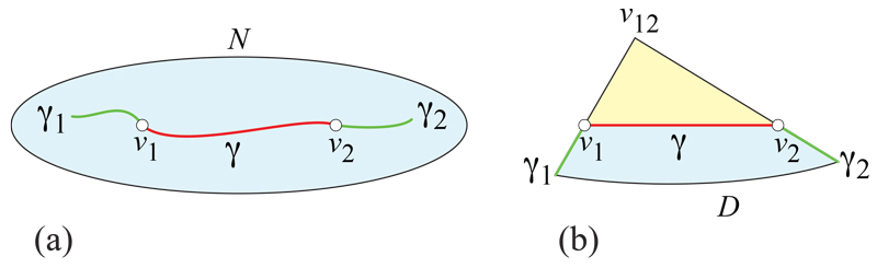
Figure 11.1: (a) Neighborhood $N$ of geodesic ${\gamma}$ connecting $v_{1}$ to $v_{2}$. (b) $N$ folded to a doubly covered domain $D$.

Proof.

Vertex merging is an intrinsic process. The proof idea below is based on a convenient way of viewing it.

Assume we executed $j$ steps from a reduction process, starting from $P$ and reaching $P_{j}$. Consider a geodesic segment ${\gamma}$ between vertices $v_{1},v_{2}\in P_{j}$ with ${\omega}_{1}+{\omega}_{2}<2\pi$. Also consider geodesics ${\gamma}_{1},{\gamma}_{2}$ starting at $v_{1}$ and $v_{2}$ such that, together with ${\gamma}$, they bisect the complete angles at $v_{1}$ and $v_{2}$, respectively. Also consider a neighborhood $N$ of the polygonal path composed by ${\gamma}_{1}$, ${\gamma}$ and ${\gamma}_{2}$, containing no vertex of $P$ excepting $v_{1},v_{2}$. See Fig. 11.1(a). Then, after merging $v_{1}$ and $v_{2}$, $N$ is isometric to a doubly covered planar domain $D$, as in (b) of the figure.

Retain the same notation for $D$. Merging the vertices $v_{1}$ and $v_{2}$ can thus be represented in the plane, by the use of $D$. There, it means extending the edges edges ${\gamma}_{1},{\gamma}_{2}$ beyond $v_{1},v_{2}$, until their intersection at $v_{12}$. So each newly created edge (say $v_{1}v_{12}$) is the extension of an edge of $D$, which derives from a geodesic on $P_{j}$ (${\gamma}_{1}$ in this case). That is, $v_{1}v_{12}$ is included in a geodesic which cannot be new from one end to the other.

Applying the previous reasoning to ${\gamma}$, which is already maximal with respect to inclusion, shows that it contains a geodesic subsegment already existing on $P_{j-1}$ and, inductively, we find a (possibly smaller) geodesic subsegment of ${\gamma}$ existing on $P$. ∎

A nearly immediate consequence of the preceding lemma is this:

Corollary 11.2.

For a polyhedron $P$ of $n$ vertices, the collection of slits (the slit graph) cuts $P$ into at most $O(n^{2})$ pieces.

Proof.

Because each slit is a geodesic segment, each pair of slits cross at most once. So the slits are pseudo-segments, subsegments of pseudo-lines. (Pseudo-lines are curves each pair of which intersects at most once, where they properly cross.) With $O(n)$ slits, the arrangement of pseudo-segments on the planar surface of $P$ has combinatorial complexity $O(n^{2})$, and in particular, has at most $O(n^{2})$ cells [AS05]. ∎

Despite the possibly quadratic complexity of the complement of the slit graph, in the end the slit graph has only $3$ or $4$ components, as established in the following lemma.

Lemma 11.3.

The slit graph of any vm-reduction process $\iota:P\to S$ has at most $n_{S}\in\{3,4\}$ components, where $n_{S}$ is number of vertices of $S$.

Proof.

Every slit $\lambda\in{\Lambda}$ is included in a geodesic ${\gamma}$ whose isometric image ${\gamma}_{j}\subset P_{j}$ creates a merge-vertex outside of $P$. With some abuse, say $\lambda={\gamma}_{j}\cap P$. By Lemma 11.1, $\lambda$ is a non-degenerate geodesic segment, hence it is included in $\partial P_{S}$. But $S$ has at most $n_{S}$ vertices, and each component of $S\setminus P_{S}$ has at least one vertex, hence $S\setminus P_{S}$ has at most $n_{S}$ components. The boundary of each component is a geodesic polygon ${\Gamma}$ (see Figure 11.2(a)), so its inverse image $\iota^{-1}({\Gamma})$ is a connected subgraph of ${\Lambda}$ containing $\lambda$. Therefore, ${\Lambda}$ has at most $n_{S}$ components. ∎

11.2 Example: Reductions of Flat Hexagon

Consider a doubly-covered regular hexagon $H=x_{1}x_{2}\ldots x_{6}$. The curvature at each vertex is $4\pi/6=2\pi/3$. We describe two different merge sequences.

Assume first that we vertex-merge vertices two-by-two in increasing order of indices, so we flatten the six original vertices and create three new vertices $x_{12},x_{34},x_{56}$, each of curvature ${\omega}_{12}={\omega}_{1}+{\omega}_{2}=4\pi/3$. The resulting surface is a doubly covered equilateral triangle of area $1.5$ times larger than the area of $H$. See Fig. 11.2(a,b). The slit graph in this case is a forest composed of three single-edge trees, every other edge of $H$. This shows that the slit graph for a vertex-merging reduction is not necessarily connected.

Note that for this example, digon-tailoring the equilateral triangle in (b) to $H$ via sculpting produces the same seals as the digon-tailoring via vertex-merging produces slits.

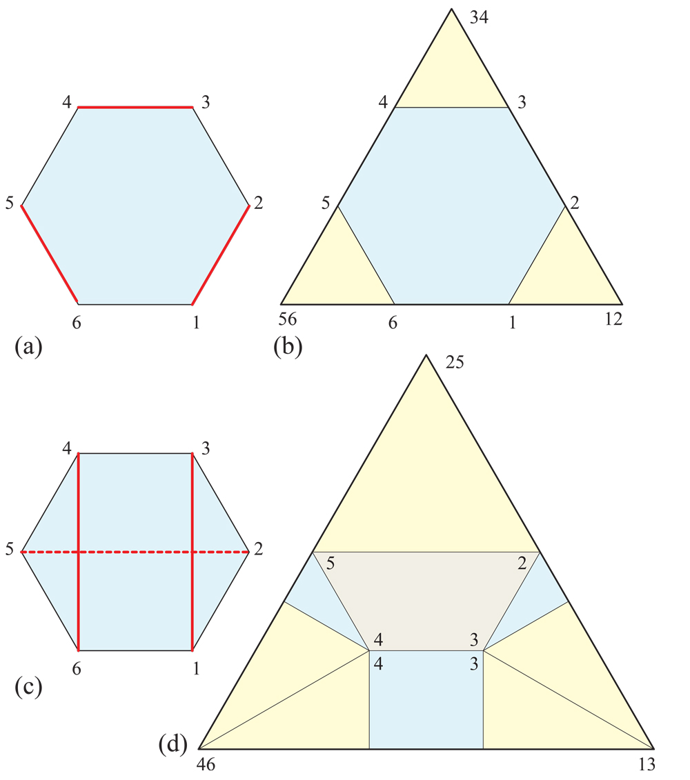
Figure 11.2: (a) Doubly-covered hexagon $H$ with slits marked (red). (b) The result after three merges. (c) Same $H$ but different merge sequence. (d) Final equilateral triangle after vertex-merging (not to same scale as (c)). Blue indicates front surface of the original $H$, tan back surface, and yellow insertions. The back face is symmetric to the front face. The images of the vertices $x_{1}$ and $x_{6}$ are on the back face, opposite to $v_{3}$ and $v_{4}$, respectively.

Notice that we cannot vertex-merge $x_{12}$ with $x_{j}$, $3\leq j\leq 6$, because the resulting curvature would be exactly $2\pi$, violating the necessary merge condition. Therefore, no matter in which order we vertex-merge the vertices $x_{3},\ldots,x_{6}$ in pairs, the resulting slit graph will be a forest of three single-edge trees. Similar reasoning shows that the slit graph for any vertex-merging reduction of $H$ is never connected.

On the other hand, for the example presented earlier in Fig. 2.6, the slit graph is a single-edge tree, hence connected. Moreover, each vm-reduction sequence of a non-isosceles tetrahedron consists of a single vertex-merging operation, yielding a doubly covered triangle. So for these surfaces, the slit graph for a vertex-merging reduction is always connected.

This leads us to consider the following question, a partial answer of which will be given in the following sections.

For which convex polyhedra does there exist a vm-reduction whose slit graph is connected?

Next we examine a different vertex-merge ordering: merging $x_{1}$ and $x_{3}$ on the front of $H$, $x_{2}$ and $x_{5}$ on the back, and $x_{4}$ and $x_{6}$ on the front. This produces another doubly covered equilateral triangle, say $T$, of area $2.5$ times larger than the area of $H$. See Fig. 11.2(c,d).

In particular, the $P$-unfolding (in the sense of Chapter 9) $H_{T}$ of $H$ onto $T$ is not simply connected, as for example, the boundary of the $v_{1}v_{3}$ slit is a non-contractible cycle; see Fig. 11.2(d). However, $H$ itself has not been disconnected by the vertex-merging slits.

Clearly for any given $P$, different vertex-merging reductions of $P$ lead to different surface areas of $S$. We leave to Open Problem 18.8 exploring bounds on, or how to achieve, the min or max surface area.

11.3 Example: Reductions of Cube

In this section we present two vm-reduction processes for the cube.

The first reduction, illustrated in Fig. 11.3, reduces the cube to a doubly covered square, which is a degenerate isosceles tetrahedron and so vm-irreducible.

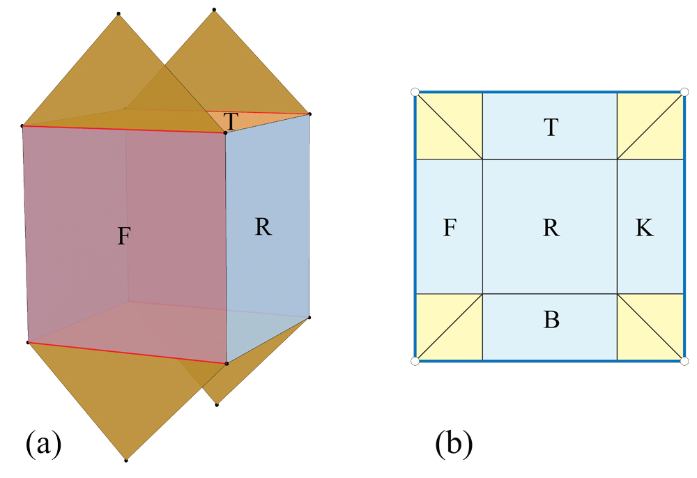
Figure 11.3: (a) A cube and its vm-reduction. (b) The corresponding vm-irreducible surface. The pattern on the back side is similar, except with $R\to L$. Inserted triangles in yellow.

In any order, slit the top front and back edges, and the bottom front and back edges, and vertex-merge their endpoints. The curvature at each cube corner is $\pi/2$, so the triangle inserts are each isosceles right triangles, a pair of which flatten the vertices to which they are incident. The slit graph is a forest of four single-edge trees.

The second merge example is more intricate; it is illustrated in Fig. 11.4, and will be revisited in Chapter 16. It reduces the cube to a doubly covered triangle, (b) of the figure. We now describe the reduction.

Figure 11.4: (a) Slits in red. Vertex merging: $1+2\to 12$. $7+8\to 78$. $5+78\to 578$. $3+12\to 123$. $4+6\to 46$. (b) The doubly covered triangle has vertices at $578,123,46$. The triangle is a right isosceles triangle. Cube surface in blue. Image of the slit graph in red.

First $v_{7},v_{8}$ are merged to produce $v_{78}$, just as in the previous example (although in (a) of the figure the triangle inserts are shown coplanar with the top $T$ of the cube). Next $v_{78}$ is merged with $v_{5}$, creating $v_{578}$. Note that the slit geodesic $v_{5}v_{78}$ crosses the slit $v_{7}v_{8}$, and so the inserted triangle pair separates the top $\triangle v_{7}v_{8}v_{78}$ (but not its mate underneath). It is not straightforward to track the consequence of each insertion.

The same two merges are mirrored on the cube bottom face $B$: $v_{1}$ and $v_{2}$, and $v_{3}$ with $v_{12}$. Finally, $v_{4}$ and $v_{6}$ are merged. So the five merges have reduced the eight cube vertices to just three: a doubly-covered triangle. It is shown unfolded in Fig. 11.4(b). Note that the three vertices of this triangle, $v_{578},v_{123},v_{46}$, are each surrounded by a polygonal domain of triangle inserts. This follows because all the cube vertices have been flattened.

The slit graph in this example has three components, satisfying Lemma 11.3.

11.4 Example: Icosahedron

We next detail using vertex-merges to reduce an icosahedron to a doubly covered triangle, without disconnecting the icosahedron surface. We will revisit and modify this example in Chapter 16, where further details will be provided.

We label the $12$ vertices of $P$ as shown in Fig. 11.5. We will merge in sequence five vertices, $v_{1},v_{2},v_{3},v_{4},v_{6}$, a merge affecting three of the triangles incident to the top vertex $v_{6}$. Symmetrically, we merge five bottom vertices, $v_{11},v_{10},v_{9},v_{8},v_{12}$. Each of these sequential merges results in a merge vertex of curvature $\frac{5}{3}\pi$, the sum of five $\frac{1}{3}\pi$ curvatures. Finally, we merge $v_{5}$ and $v_{7}$, cutting across the middle band of triangles, creating a merge vertex of curvature $\frac{2}{3}\pi$. (So the total curvature is $(\frac{5}{3}+\frac{5}{3}+\frac{2}{3})\pi=4\pi$, satisfying the Gauss-Bonnet theorem.) The resulting doubly covered triangle $abc$ has angles $30^{\circ},30^{\circ},120^{\circ}$.

Figure 11.5: Labels $i$ for vertices $v_{i}$.

Figure 11.6: Four geodesic slits on $P$, each entering $P$ at $m^{\prime}_{i}$. $v_{6}$ is the top vertex of $P$.

We now detail the top sequential merge of five vertices. Each of the four merges $i$ is accomplished by inserting two copies of a triangle $T_{i}$, whose apex is the merge vertex $m_{i}$.

$$v_{1}+v_{2} \to m_{1}\;,\;T_{1}$$

$$m_{1}+v_{3} \to m_{2}\;,\;T_{2}$$

$$m_{2}+v_{4} \to m_{3}\;,\;T_{3}$$

$$m_{3}+v_{6} \to m_{4}\;,\;T_{4}\;.$$

(Here we are using ‘$+$’ and ‘$\to$’ informally to mean ‘merge’ and ‘creating’ respectively.) The merge of $m_{i}$ to the next vertex $v_{i+2}$ slits a geodesic ${\gamma}_{i+1}$ from $m_{i}$, down one copy of $T_{i}$, onto $P$ at the point we call $m^{\prime}_{i}$. This geodesic crosses the previous geodesic cut ${\gamma}_{i}$ from $m_{i-1}$ to $v_{i+1}$ at $m^{\prime}_{i}$. So $m^{\prime}_{i}$ is a point on $P$, whereas $m_{i}$ is not on $P$, but rather on $P_{i}$, the intermediate polyhedron after the $i$-th merge. In Fig. 11.6 illustrates the four merge cuts on $P$, with just $T_{1}$ shown to illustrate ${\gamma}_{2}$ crossing from $T_{1}$ onto $P$ at $m^{\prime}_{1}$.

Returning to Fig. 11.5, we merge five vertices on the top side of $P$, and symmetrically five on the bottom side, and two connecting across the “equitorial” band of triangles. These merges reduce the original $12$ vertices to $3$, so the result is a doubly covered triangle. The slit graph is a forest of three trees.

The resulting doubly covered triangle $abc$ is shown in Fig. 11.7, cut open so that both sides can be seen. It may not be obvious, but the white regions in Fig. 11.7 form a non-overlapping net of the icosahedron, when, for example, the doubly-covered triangle is cut along edges $ac$ and $bc$ as illustrated.

Figure 11.7: Icosahedron surface is white, triangle inserts (merge domains) colored. $\triangle abc^{\prime}$ is the back side of $\triangle abc$, with $c=c^{\prime}$ identified.

11.5 Example: Hexagonal Shape with Cycle

The next example shows that the slit graph could have a cycle. $P$ is the convex hull of two similar hexagons in parallel planes, separated by a distance $h$. Label the top hexagon with vertices $v_{1},\ldots,v_{6}$, and the larger base hexagon $x_{1},\ldots,x_{6}$. See Fig. 11.8.

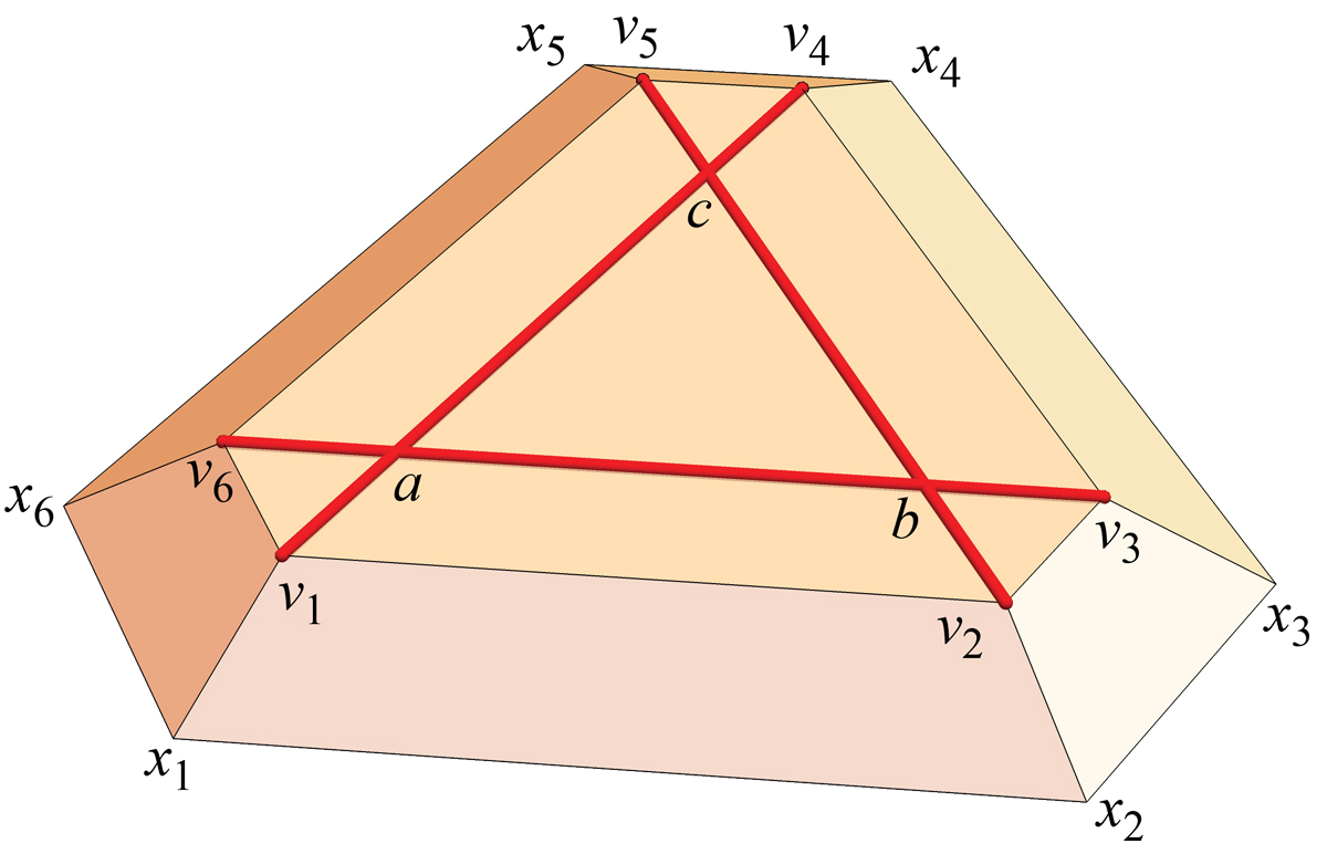
Figure 11.8: Three vertex-merge slits (red) will form a cycle $abc$.

Note that as $h\to 0$, the curvature ${\omega}(v_{i})\to 0$. Let $h={\varepsilon}$ be a small positive height, so ${\omega}={\omega}(v_{i})$ is small.

Now we are going to merge $v_{1}+v_{4}$, then $v_{2}+v_{5}$, and finally $v_{3}+v_{6}$, where again $+$ means “merge.” The merge of $v_{1}$ and $v_{4}$ is accomplished by a pair of triangles with angles ${\omega}/2,{\omega}/2,\pi-{\omega}$. With ${\omega}$ small, the inserted digon $D(v_{1},v_{4})$ is very narrow, akin to a “fat” edge with endpoints $v_{1}$ and $v_{4}$. Then the geodesic between $v_{2}$ and $v_{5}$ crosses near $c$ over $D(v_{1},v_{4})$, but because that is narrow, the geodesic does not look too different from the $v_{2}v_{5}$ edge illustrated in the figure—the geodesic “jags” slightly as it crosses $D(v_{1},v_{4})$. Again the digon $D(v_{2},v_{5})$ is narrow, and so does not greatly deviate the geodesic from $v_{3}$ to $v_{4}$, which now crosses both previously inserted digons, near $b$ and $a$.

After these three vertex-merges, $P_{3}$ is a 9-vertex polyhedron. It should be clear that the roughly triangular region $abc$ in the figure is disconnected by the three slits, which form a cycle in ${\Lambda}_{3}$. Further slits cannot “repair” the disconnecting cycle, so the final ${\Lambda}$ will have at least one cycle.

This leads us to consider the following question: For which convex polyhedra do there exist vm-reductions whose slit graphs have no cycle? Although we pursue this question in subsequent chapters, it remains unresolved. See Open Problem 18.9.

11.6 Vertex Merging and Unfoldings

The goal of this section if to relate vm-reductions and their slit graphs to unfoldings.

An unfolding of a convex polyhedron $P$ cuts the surface along a spanning tree of the vertices, producing a polygon $U_{P}$ when developed in the plane. See, e.g., [O’R13]. When that polygon is simple—non-self-intersecting, i.e., non-overlapping—then $U_{P}$ is called a net for $P$, i.e., an injective embedding of $P$ into the plane.

Consider a reduction process $\iota:P\to S$ of $P$ onto the vm-irreducible surface $S$. Then $P_{S}=\iota(P)\subset S$ is an unfolding of $P$ onto $S$ in the sense of Chapter 9. Further unfolding $S$ to the plane (there are in general many ways to do this) provides an unfolding $U_{P}$ of $P$ in the plane.

We recall here some definitions for subsets related to convex polyhedra.

• A simple closed curve is a closed curve without self-intersections (i.e., homeomorphic to a circle).

• A (geodesic) polygon is a simple closed curve composed of (geodesic) segments.

• A domain is a connected open set.

• A polygonal domain is a the closure of a domain whose boundary is a finite union of polygons.

• A simple polygonal domain is a polygonal domain with one boundary component.

• By a simply connected set we understand a set each path-connected component of which is contractible; so the set itself is not required to be connected.

Lemma 11.4.

Consider a partial vm-reduction $\iota_{j}:P\to P_{j}$, for some $1\leq j\leq k$, and identify, for simplicity, $P=\iota_{j}(P)\subset P_{j}$. Every component of $P_{j}\setminus P$ is a simple polygonal domain containing precisely one vertex. In particular, the conclusion holds for $S\setminus P_{S}$, where $S$ is the vm-irreducible end result of the reduction process.

We have seen this lemma verified for $S\setminus P_{S}$ in the series of examples above: Figs. 11.2(b,d), 11.3(b), 11.4(b), and 11.7.

Proof.

The proof is a simple induction on the step $m$ of the vm-reduction sequence.

At step $m=1$, we merge the first two vertices of $P$, and $P_{1}\setminus P$ consists of precisely the pair of inserted triangles, with one vertex, the shared apex of those triangles, outside $P$.

Notice that each (partial) vm-reduction $\iota_{j}$ yields a forest $F$ of binary rooted trees, every node of which is a vertex in some $P_{l}$, with $1\leq l\leq j$. (These vertex trees are not to be confused with slit trees.) After a complete reduction, the $3$ or $4$ vertices of $S$ are the roots of the $3$ or $4$ vertex-trees that were merged to produce those root vertices. Precisely, the leaves of $F$ are the vertices of $P$, and two nodes in $F$ have a common parent if and only if they are merged at some step $l$. If a vertex $v\in P$ has not been merged, it is an isolated node of $F$. If $v$ has been merged, then it has been flattened: ${\omega}(v)=0$.

Assume now that the conclusion holds for the first $m-1$ steps. At step $m$ we merge, say, the nodes $n_{1}$ and $n_{2}$ of $F$, along the geodesic segment ${\gamma}$ in $P_{m-1}$. Note $n_{i}$ could be a vertex of $P$, or a vertex in a domain of $P_{m-1}\setminus P$ resulting from a merge. If $n_{i}$ is a vertex of $P$, then it is not surrounded by a polygonal domain; for simplicity, we assume in this case that the polygonal domain is $\{n_{i}\}$ itself. Cutting along ${\gamma}$ and inserting the curvature triangles merges the simple polygonal domains around $n_{1}$ and $n_{2}$ into a larger simple polygonal domain, containing precisely the resulting node $n_{12}$. ∎

For example, in Fig. 11.4, when $n_{1}=v_{5}$ and $n_{2}=v_{78}$, the domain around $v_{78}$ (yellow in (b) of the figure) is merged with the new curvature triangles (tan) to form one simple polygonal domain containing $n_{12}=v_{578}$. In Fig. 11.7, the domains around triangle vertices $a$ and $b$ are the result of four merges, colored in the figure.

Theorem 11.5.

Consider a reduction process $\iota:P\to P_{S}\subset S$ of $P$ onto the vm-irreducible surface $S$, resulting in slit graph ${\Lambda}$.

• If ${\Lambda}$ is a forest of trees then $P_{S}$ is a polygonal domain in $S$.

• If ${\Lambda}$ is connected then $P_{S}$ is simply connected.

• If ${\Lambda}$ is a tree then $P_{S}$ is a simple polygonal domain in $S$.

Proof.

Each slit in ${\Lambda}$ appears twice in the boundary of $P_{S}$, once for each bank. Since $P$ has no boundary, the whole boundary of $P_{S}$ is produced in this way, hence it is a finite union of segments.

It also follows that each tree component of ${\Lambda}$ yields a boundary component of $P_{S}$, which is a polygon. Therefore, if ${\Lambda}$ is a tree then $P_{S}$ is a simple polygonal domain in $S$. And if ${\Lambda}$ is a forest of trees then $P_{S}$ is a polygonal domain.

If a connected component of $P_{S}\subset S$ is not simply connected then it has several boundary components, impossible if ${\Lambda}$ is connected. ∎

Next we offer a topological viewpoint. View $P$ as a topological sphere with conical-point vertices. A vertex-merge of $v_{1}$ and $v_{2}$ is a topological-circle hole cut in $P$, passing through $v_{1},v_{2}$, which is then filled with a topological disk—the two back-to-back triangles with a new vertex $v$ inside the disk. Two connected vm-slits on $P$ correspond topologically to merging two holes to one hole. A tree of vm-slits is then topologically a single hole, filled with doubly-covered triangles. Thus a forest of trees is topologically a collection of disjoint holes on $P$. As all holes are bounded by geometric segments, the result is a polygonal domain with polygonal holes.

Assume now that ${\Lambda}$ is a tree, so $P_{S}$ is a simple polygonal domain in $S$ by Theorem 11.5, where $S$ a doubly-covered triangle or an isosceles tetrahedron. With an appropriate unfolding of $S$, $P_{S}$ remains connected and thus becomes an unfolding of $P$ in the plane. However, the unfolding may overlap, and so not constitute a net. This is explained in the next section.

11.7 Unfolding Irreducible Surfaces

Assume we have a vm-reduction $\iota:P\to P_{S}\subset S$ resulting in a tree slit graph ${\Lambda}$ so that $P_{S}$ is a simple polygonal domain of $S$, by Theorem 11.5. We explore next the question of unfolding $S$ to the plane, preserving connectedness of $P_{S}$. We start with $S$ a doubly-covered triangle.

11.7.1 $S$: Doubly-covered Triangle

Let $u_{1},u_{2},u_{3}$ be the three vertices of $S$. Each is surrounded by polygonal domains $M_{1},M_{2},M_{3}$ created by repeated triangle inserts. Two examples of these domains are the cube vm-reduction in Fig. 11.4(b) and the icosahedron vm-reduction in Fig. 11.7. Both are displayed with their triangles cut open.

Now we argue that $S$ can be cut open via a spanning tree without disconnecting $P$. So this provides an unfolding of $S$ that preserves $P$ as a single piece, as in those two figures. Although we can guarantee a single piece, we have not established this piece is a net, avoiding overlap. See Open Problem 18.10.

Topologically, $S$ is a sphere with three conical points / vertices $u_{i}$, each surrounded by a merge-domain $M_{i}$, with the remainder of $S$ the original $P$: in loose notation, $P=S\setminus\left(\cup_{i}M_{i}\right)$. Each $M_{i}$ is topologically a disk, as depicted in Fig. 11.9(a).

There are only two combinatorially distinct spanning slit trees for unfolding $S$: a path $u_{1},u_{2},u_{3}$ (and its index permutations), or a Y-tree: some point $x$ in $P$ with slits from $x$ to each $u_{i}$. (In both Figs. 11.4(b) and 11.7, the slit tree is a path.) For either spanning tree, a slit path $\rho$ must enter $M_{i}$ to reach $u_{i}$, and in the path case, the slit path must also exit $M_{i}$.

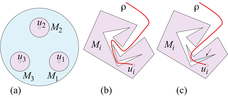
Figure 11.9: (a) Topology of $S$. (b,c) Slit path $\rho$ to $u_{i}$. In (c), the marked region is disconnected from $P$.

Because each $M_{i}$ is a disk, there is a $\rho$ that crosses $\partial M_{i}$ just once on entrance, and in the path case, once again on exit. Fig. 11.9(b) illustrates such a one-cross $\rho$. Fig. 11.9(c) shows that, if $\rho$ crossed $\partial M_{i}$ at more than one point, then a piece of $P$ is disconnected. But because the spanning slit tree can be chosen to avoid the (c) situation, we are guaranteed that we can unfold $S$ to the plane so that $P\subset S$ remains a simply connected polygonal domain in the plane.

11.7.2 Net and Overlap

Let us temporarily ignore the structure of $S=P\cup\left(\cup_{i}M_{i}\right)$, and just view $S$ as a doubly covered triangle $\triangle$. If, for every spanning slit tree $T$, the unfolding of $\triangle$ avoids overlap, then we immediately have that the unfolding of $P$ avoids overlap, and so we have found a net for $P$.

Alas, this is not true for every $T$, as the example in Fig. 11.10 shows.

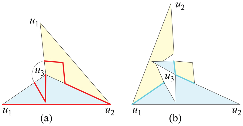
Figure 11.10: (a) Front: blue; back: yellow. Slit path $T$: $(u_{1},u_{2},u_{3})$. (b) Unfolding after cutting $T$. Blue segments remain uncut.

In (a) the $u_{2},u_{3}$ slit path spirals around $u_{3}$ from the back to the front. The unfolding is shown in (b), with the uncut segments highlighted, showing clear overlap.

Although this may seem a contrived example, the merge regions $M_{i}$ might be created from spiraling slit trees, as we will discuss in the the following chapters, and could be quite complex, as the icosahedron example (Fig. 11.7) suggests. A natural slit path follows the merge vertices into each $M_{i}$ region: $\mu=(m_{0},m_{1},m_{2},\ldots,m_{i})$, where $m_{0}=u_{1}$. However, we leave it as an open question (Open Problem 18.10) of whether forming a slit tree by following $\mu$ for each $M_{i}$—or any other slit tree—unfolds $P$ to a net.

11.7.3 $S$: Isosceles Tetrahedron

Vertex-merging could result in an isosceles tetrahedron $S$ (rather than a doubly covered triangle). This occurred in the first cube reduction, illustrated in Fig. 11.3(b). This does not change the topological picture Fig. 11.9(a) significantly: just a fourth merge-domain disk $M_{4}$ is added, and there are two more possible spanning tree structures. Therefore, by similar reasoning, we can ensure a single-piece unfolding of $P$ to the plane. But again, we leave open the question of whether there is always a slit tree that leads to a nonoverlapping single piece, a net for $P$.

Chapter 12 Planar Spiral Slit Tree

The previous chapter showed that if the slit graph ${\Lambda}$ of a vm-reduction is a tree, then we can unfold $P$ to the plane, and possibly to a non-overlapping net. So we have made a goal of finding a vm-reduction ordering that results in ${\Lambda}$ a tree. Our overall plan is to partition $P$ into two “halves” via a simple closed quasigeodesic $Q$, and then to vm-reduce the vertices in each half separately. (As mentioned in Chapter 10, such quasigeodesics always exist.) Let $V$ be the set of vertices inside $Q$. We will eventually show (in Chapter 15) how to vertex-merge all of $V$ so that the slit graph of that half is a tree. In this chapter we illustrate the main idea by assuming $V$ lies in a plane.

12.1 Sequential Spiral Merge

Let $V=\{v_{1},v_{2},v_{3},\ldots,v_{n}\}$ be the vertices in the above-half $P^{+}$ of polyhedron $P$. Define a sequential merge as a series of vertex-merges where at each step, the previous merge vertex is connected to a vertex of $V$. Thus the merge region—the union of all the triangle inserts—grows a single connected domain enclosing, in the end, one vertex by Lemma 11.4.

There are many possible sequential merge orders. We choose one that we call a spiral merge. See ahead to Fig. 12.5 for why “spiral” is an appropriate term. In the planar situation, we view vertices as having zero curvature, so that $P^{+}$ becomes planar. In this context, a slit is a line segment $s$, wholly in $P$. Each triangle insert degenerates to just $s$, and creates a merge vertex somewhere along $s$. We will show in Theorem 12.1 that a spiral merge algorithm in two dimensions results in ${\Lambda}$ a slit tree.

12.2 Notation

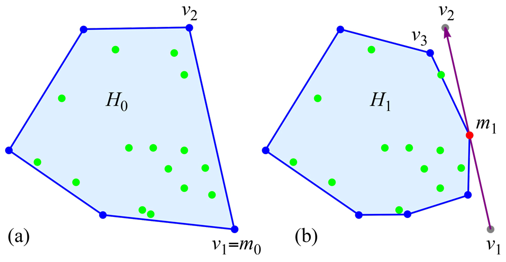
Figure 12.1: $v_{1}$ is merged with $v_{2}$ to produce $m_{1}$. $H_{1}={\rm conv}(V_{1})$ where $V_{1}=V_{0}\setminus\{v_{1},v_{2}\}\cup m_{1}$.

The detailed argument needs considerable notation beyond that introduced earlier, which we gather below for reference.

• $V=V_{0}=\{v_{1},v_{2},v_{3},\ldots,v_{n}\}$: Vertices in the plane. (Later (in Chapter 15) these will be vertices on the surface of the polyhedron $P$.)

• $m_{i}$: merge vertex, the vertex created by merging $m_{i-1}$ with $v_{i+1}$ with $m_{0}=v_{1}$. We sometimes abbreviate this as $m_{i-1}+v_{i+1}\to m_{i}$.

• $s_{i}=m_{i-1}v_{i+1}$. The $i$-th slit/merge segment. The new merge vertex $m_{i}$ lies on $s_{i}$.

• So each slit segment has three labeled points: $m_{i-1},m_{i},v_{i+1}$.

• $v_{1}$ is also given the label $m_{0}$, so $s_{1}=v_{1}v_{2}=m_{0}v_{2}$.

• $m_{i}$ can lie anywhere along $s_{i}$. In Figs. 12.1-12.5, $m_{i}$ was chosen at a random point on $s_{i}$.

• ${\Lambda}_{i}=\cup_{i}s_{i}$ is the slit graph after the $i$-th merge. ${\Lambda}$ is the full slit graph.

• $v_{i}$ is called flattened if it has already been merged. (In Chapter 15, when $v_{i}$ is a vertex of positive curvature, the merge will reduce $v_{i}$’s curvature to zero.)

• $V_{i}$ is the set of not-flattened vertices remaining after the $i$-th merge $s_{i}=m_{i-1}v_{i+1}$. $m_{i}\in V_{i}$. $|V_{i}|$ is the number of vertices in $V_{i}$.

• $H_{i}$ is the convex hull of $V_{i}$. We view $H_{i}$ as a closed region of the plane and $\partial H_{i}$ its boundary, a convex polygon. $H_{0}$ is the convex hull of $V=V_{0}$.

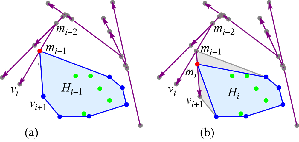
Figure 12.2: General step: $i$-th merge. (a) $s_{i-1}=m_{i-2}v_{i}$. $s_{i-1}\cap H_{i-1}=m_{i-1}$. (b) $s_{i}=m_{i-1}v_{i+1}$. $s_{i}\cap H_{i}=m_{i}$. $s_{i-1}\cap s_{i}=m_{i-1}$.

12.3 Algorithm Description

First merge.

The algorithm starts by selecting any edge of the convex hull $H_{0}$ of $V=V_{0}$, say $v_{1}$ and $v_{2}$, and merging them via the merge segment $s_{1}=v_{1}v_{2}$. In the plane, this amounts to replacing $v_{1}=m_{0}$ and $v_{2}$ with with a new vertex $m_{0}+v_{2}\to m_{1}$ on the segment $s_{1}$. The merge flattens $v_{1}$ and $v_{2}$, which is why they are removed. $V_{1}=V\setminus\{v_{1},v_{2}\}\cup m_{1}$, and $H_{1}={\rm conv}(V_{1})$. See Fig. 12.1.

Second merge.

Next, $m_{1}$ is merged with the first vertex beyond $m_{1}$ on $H_{1}$. Call this vertex $v_{3}$. Note that $v_{3}$ might not be the next vertex after $v_{2}$ on $H_{0}$, because $V_{1}\neq V_{0}$ and so $H_{1}\neq H_{0}$. The merge of $m_{1}$ and $v_{3}$ introduces a new merge vertex $m_{2}$ on $s_{2}=m_{1}v_{3}$, and both $m_{1}$ and $v_{3}$ are flattened and removed from $V_{1}$, while $m_{2}$ is added, to produce $V_{2}$.

General step.

The $i$-th merge connects $m_{i-1}$ to $v_{i+1}$, where $v_{i+1}$ is the next vertex on $H_{i-1}$ beyond $m_{i-1}$. See Fig. 12.2. Then $m_{i}$ lies on $s_{i}=m_{i-1}v_{i+1}$, the vertex set is updated as $V_{i}=V_{i-1}\setminus\{m_{i-1},v_{i+1}\}\cup m_{i}$, and $H_{i}={\rm conv}(V_{i})$. Note that $|V_{i}|=|V_{i-1}|-1$, because two vertices are removed (flattened) and one added. But $\partial H_{i}$ does not bear a similar relation to $\partial H_{i-1}$ because the new hull may wrap around vertices that were strictly interior to $H_{i-1}$ (green in the figures).

Completion.

The process continues until all the original $v_{i}$ vertices are merged, leaving just one vertex $V_{n-1}=\{m_{n-1}\}$. A full trace is illustrated in Fig. 12.3. (The reason there are $n-1$ merges rather than $n$ is that the first merge flattens two vertices of $V$, while all subsequent merges flatten two vertices but only one is from $V$.)

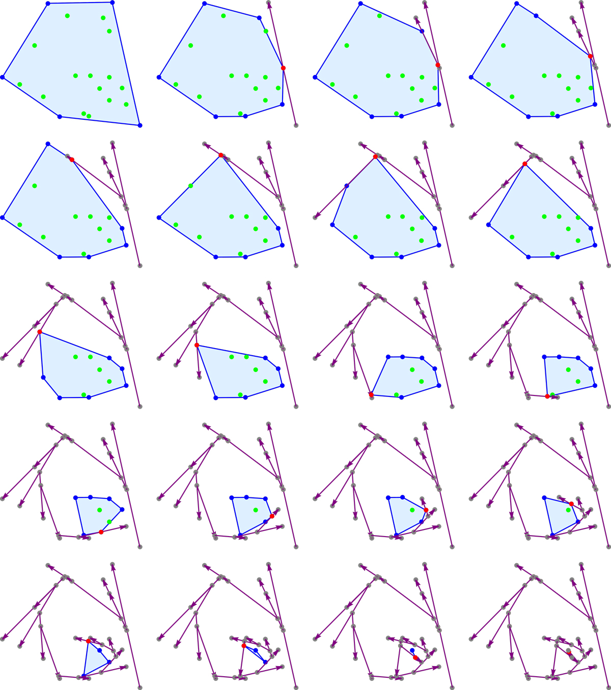
Figure 12.3: Trace of example with $|V|=20$, from which Figs. 12.1 and 12.2 are details.

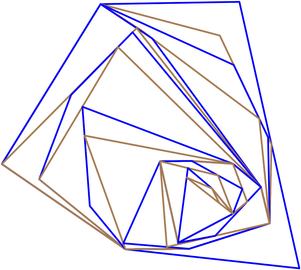
Figure 12.4: Nested $H_{i}$ for all $i$, from Fig. 12.3, alternately colored blue and brown.

12.4 Planar Proof

We first assume that all points—both vertices in $V$ and merge points $m_{i}$—are in general position in the sense that no three are collinear. Later we will see that allowing collinearities does not change the main claim that ${\Lambda}=\cup_{i}s_{i}$ is a tree.

The induction hypothesis consists of several claims:

1. $H_{i}$ is nested inside $H_{i-1}$: $H_{i-1}\supset H_{i}$. See Fig. 12.4.

2. $s_{i}$ only intersects $H_{i}$ in one point, the merge vertex: $s_{i}\cap H_{i}=\{m_{i}\}$. See Fig. 12.2(b).

3. Consecutive slit segments share just one point, an endpoint of the later segment: $s_{i-1}\cap s_{i}=\{m_{i-1}\}$. See Fig. 12.2.

4. The set of vertices reduces by one each iteration: $|V_{i}|=|V_{i-1}|-1$, for $i>1$.

5. ${\Lambda}_{i}$ is a tree.

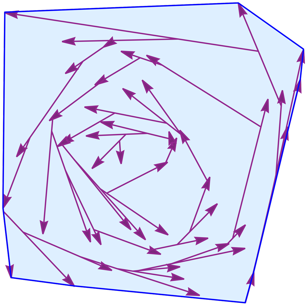
Figure 12.5: ${\Lambda}$ for a set of $|V|=50$ vertices. Only slit segments are shown.

Basis.

These claims are easy to see for $i=1,2$, just by construction according to the algorithm. Neverthless, just for completeness, we run through the basis. Refer to Fig. 12.1.

1. $H_{0}\supset H_{1}$ because the edge $v_{1}v_{2}$ is replaced by a point $m_{1}$ on that edge.

2. $s_{1}\cap H_{1}=\{m_{1}\}$ by construction.

3. For $i=1$, there is just one segment $s_{1}$. $s_{2}$ starts at $m_{1}\in s_{1}$, so indeed $s_{1}\cap s_{2}=\{m_{1}\}$.

4. $V_{1}$ has one fewer vertex than does $V=V_{0}$ because two ($v_{1}$ and $v_{2}$) are removed and one ($m_{1}$) is added.

5. ${\Lambda}_{1}=s_{1}$ is a single-edge tree.

General Step.

Assume the induction hypotheses are satisfied up to $i-1$, and consider the $i$-th merge. It will help to consult Fig. 12.2, where (a) is established by the induction hypothesis, and (b) reflects the situation to be proved. The algorithm chooses $v_{i+1}$ as the next vertex on $H_{i-1}$, so $s_{i}=m_{i-1}v_{i+1}$ is an edge $e$ of $\partial H_{i-1}$.

1. $H_{i-1}\supset H_{i}$ because the edge $e$ is replaced by the merge vertex $m_{i}$.

2. $s_{i}\cap H_{i}=\{m_{i}\}$ by construction.

3. $s_{i-1}\cap s_{i}=\{m_{i-1}\}$ by construction.

4. $|V_{i}|=|V_{i-1}|-1$, again because $V_{i}=V_{i-1}\setminus\{m_{i-1},v_{i+1}\}\cup\{m_{i}\}$.

5. ${\Lambda}_{i}$ is a tree. By (3) above, $s_{i}$ has an endpoint $m_{i-1}$ on $s_{i-1}$, and otherwise does not intersect $s_{i-1}$. It remains to prove that the interaction of $s_{i}$ with the earlier segments in ${\Lambda}_{i}$ maintains the tree property. In fact, we show that $s_{i}\cap s_{j}=\varnothing$ for $j<i-1$.

   As we’ve seen, $s_{i}$ is an edge $e$ of $\partial H_{i-1}$, and from (1) we know that $H_{j}\supset H_{i-1}$ for $j<i-1$. From (2), each $s_{j}$ intersects $H_{j}$ in just one point $m_{j}$, which is removed from $V_{j}$ in the next step. So $s_{j}$ is disjoint from $H_{j+1}={\rm conv}(V_{j})$. And so $s_{j}$ cannot intersect $s_{i}$, which is an edge of $\partial H_{i-1}$.

   Therefore, we have shown that $s_{i}$ just intersects ${\Lambda}_{i-1}$ at the one point $m_{i-1}$, and so maintains the tree structure for ${\Lambda}_{i}$.

The tree structure is illustrated in Fig. 12.5. It is in a sense a geometric directed binary tree, spiraling from the boundary of $H_{0}$ into the center.

Collinearities.

If there are collinearities, then several consecutive segments can collinearly overlap. So it could be, for example, that $s_{i-1}=m_{i-2}v_{i}$ overlaps with $s_{i}=m_{i-1}v_{i+1}$ in the portion from $m_{i-1}$ to $v_{i}$. Thus several slit segments could collinearly overlap with an edge of $H_{i}$. If we union each group of collinearly overlapping segments to one segment, then all the properties claimed in the induction hypothesis continue to hold, although different notation would be required to capture the unioning of several collinearly overlapping segments into one.

Theorem 12.1.

For any set $V$ of vertices in the plane, the sequential merging algorithm detailed in Section 12.3 results in a slit graph ${\Lambda}$ that is a tree (see Fig. 12.5).

As the figures suggest, we have implemented this algorithm.

Convexity and, in particular, the convex hull, plays an essential role in this algorithm. Before we can apply the same overall idea to a set $V$ on a three-dimensional $P^{+}$ in Chapter 15, we need to explore convexity and convex hulls on $P$. This is the topic of the next chapter.

Chapter 13 Convexity on Convex Polyhedra

We’ve set as our goal proving that there is a vm-reduction ordering of the vertices $V$ inside a quasigeodesic $Q$ that results in a slit tree ${\Lambda}$, a goal achieved in Chapter 15. Before we reach that point, we need to develop a clear notion of what constitutes the convex hull of $V$. This in turn requires a clear notion of convexity on polyhedral convex surfaces, which is our focus in this chapter.

Our investigation into convexity on convex polyhedra is, to our knowledge, the first in this direction, and seems to have a rich potential. We barely touch on some classical convexity results (such as Helly’s and Radon’s theorems: Examples 13.13 and 13.22), and do not attempt to provide their adaptations in this new theory of convex sets. Instead we focus on developing basic facts that ultimately lead to a characterization of the “relative convex hull” of a set of vertices inside a simple closed quasigeodesic $Q$ (Section 13.10).

We first argue that, for our purposes, the proper notion of a convex set $S$ is one that includes every geodesic segment between points in $S$, in contrast to, say, including at least one geodesic segment. Defining the convex hull of a set of vertices $V$ as the smallest convex set including $V$ (Section 13.6) leads to some surprising and perhaps undesirable properties. For example, the convex hull of a set inside $Q$ does not always remain inside $Q$ (Example 13.30). These properties lead us to develop a notion of “relative” convexity, and the relative convex hull in Section 13.9. Among our main results is Theorem 13.40, which characterizes the relative convex hull of vertices inside a quasigeodesic $Q$. This characterization is then employed in Chapter 15.

Because of the many lemmas and details in this long chapter, we offer a concise summary of $38$ individual results in Section 13.10.

Throughout, for a set $S$, we use $\partial S$ for its boundary, and $\mathring{S}$ and $\bar{S}$ for the interior and closure of $S$ respectively.

13.1 Convex Curves

Let $C$ be a simple, closed, curve on the surface of a convex polyhedron $P$. We will assume $C$ is polygonal, turning at corners which in general may or may not be vertices of $P$ (although we’ll continue to use labels $v_{i}$). View $C$ as directed counterclockwise from above. At each corner $v_{i}$ of $C$, let ${\alpha}_{i}$ be the surface angle to the left, and ${\beta}_{i}$ the angle to the right. $C$ is called a convex curve if ${\alpha}_{i}\leq\pi$; all such angles are convex angles. Angles ${\beta}_{i}$ strictly greater than $\pi$ are called reflex.

If $C$ also satisfies ${\alpha}_{i}\leq{\beta}_{i}$, we call it an ${\alpha}{\beta}$-convex curve. If ${\alpha}_{i}<{\beta}_{i}$ for all (non-zero curvature) corners, it is a strictly ${\alpha}{\beta}$-convex curve.

A simple, closed quasigeodesic $Q$ is a curve $C$ that is convex to both sides: ${\alpha}_{i}\leq\pi$ and ${\beta}_{i}\leq\pi$. By a theorem of Pogorelov [Pog49], every convex polyhedron has at least three such quasigeodesics.

In general, quasigeodesics are not ${\alpha}{\beta}$-convex to either side. The total curvature of the vertices to either side of $Q$ is $\leq 2\pi$, and only equal to $2\pi$ if $Q$ is a geodesic, passing through no vertices, a fact we use later.

A geodesic polygon is a polygon whose edges are geodesic arcs. A geodesic-segment polygon is a polygon whose edges are geodesic segments, i.e., shortest paths. The distinction between these two types of polygons plays a significant role in this chapter. For brevity, we will frequently abbreviate “geodesic arc” with “geoarc,” and “geodesic segment” with “geoseg.” Although we are mainly interested in convex sets contained within polygons, a convex curve could include smoothly curved arcs.

13.2 Notions of Convexity

Several notions of convexity have been employed so far on surfaces, see for example [Ale78], [Ban81], [GM01], [Mit16], [Zam91], and the references therein. We have not made a comprehensive accounting of all the different definitions found in the literature, and instead mention next only three.

A subset $S$ of $P$ is said to be

• geodesically convex if, given any two points in $S$, there is a unique geodesic segment joining them in $S$; [Udr13].

• totally convex if any geodesic which joins two points of $S$ is contained in $S$; [Ban81].

• metrically convex if, given any two points in $S$, there is at least one geodesic segment joining them in $S$; [GM01].

We should mention that there is variation in the literature. For example, [Vis18] uses the term “geodesically convex” to mean what we list above as “totally convex.”

Geodesic convexity is not suitable for our framework, because an open geodesically convex set could contain no vertex $v$—two geodesic segments would wrap around $v$. Since our main concern is with geodesic segments forming a slit graph, total convexity, which focuses on geodesics (not necessarily shortest paths), is also inappropriate.

We will need a notion of a convex hull of a set of points $V$ on $P$. In analogy with the Euclidean case, we would like to define the convex hull of $V$ to be the intersection of all convex sets containing $V$. We next indicate why the natural metric convexity, and in particular, its “at least one geodesic segment” criterion, is not the correct version in our context.

Example 13.1.

Let $\Delta$ be a doubly-covered triangle $v_{1}v_{2}v_{3}$, with $V=\{v_{1},v_{2},v_{3}\}$. The front triangle is a metric-convex set containing $V$, as is the back triangle. So the metric-convex hull of $V$ consists of the three edges $v_{1}v_{2}$, $v_{2}v_{3}$, $v_{3}v_{1}$. However, one would expect to obtain $\Delta$ as the convex hull of its vertices, as we do in Theorem 13.32. Moreover, the situation illustrated by the doubly-covered triangle could be troublesome in some specific situations as well. We address these situations in Section 13.6 below.

13.3 Ag-convexity

Define $S$ to be ag-convex—all-geodesics convex—if every geodesic segment between two points of $S$ is in $S$. In the following we will focus on ag-convexity, which we henceforth abbreviate as, simply convexity.

This same notion of convexity has been used in different contexts, see for example [AKP19] and [LP21], although we have not seen it applied to convex polyhedra. Other types of convexity will be specifically identified to differentiate them from ag-convexity.

Clearly, every convex set is path-connected, but one can say more.

Lemma 13.2 (Classification).

Let $S$ be a closed convex set on $P$. Then $S$ is either a point, or a geodesic arc, or a simple closed geodesic, or it has interior points.

Proof.

Assume $S$ contains two distinct points, hence it contains a geodesic segment ${\gamma}$. Assume ${\Gamma}$ is the maximal (with respect to inclusion) geodesic in $S$ including ${\gamma}$; so it could be an arc, or a simple closed curve. If the image set of ${\Gamma}$ is $S$, we are done. (Here the image set of ${\Gamma}$ is the set of points on $P$ comprising the curve.)

Assume there exists a point $x$ in $S$ but not on ${\Gamma}$. Join it with an interior point $y$ of ${\Gamma}$, say with the geodesic segment ${\gamma}_{y}$. Locally around ${\gamma}_{y}$ the set $S$ is flat, so moving $y$ continuously on ${\Gamma}$ provides a continuous family of geodesic segments ${\gamma}_{y}$, all included in $S$. Therefore $S$ has interior points. ∎

Example 13.3.

The whole surface $P$ is obviously convex. We also consider the empty set and the single-point sets to be convex.

Example 13.4.

Notice that the closure of a convex set is not necessarily convex. The interior of a face of a doubly-covered triangle is convex, while the whole face is not, because two points on different edges of the triangle are connected by geodesic segments on both sides of the triangle.

We’ll repeatedly use the following simple fact.

Lemma 13.5 (Local behaviour).

Let $S\subset P$ be a convex set and $x\in S$. Then there exists a small ball $B_{x}$ around $x$ such that $S\cap B_{x}$ is isometric either to a planar convex set (if $x$ is not a vertex of $P$), or to a convex set on a cone of apex $x$.

Proof.

Just choose $B_{x}$ around $x$ to include no vertices of $P$ (other than possibly $x$), and notice that $S\cap B_{x}$ is still convex on $B_{x}$. ∎

Recall from Section 13.1 that an ${\alpha}{\beta}$-convex curve is a strictly ${\alpha}{\beta}$-convex curve if ${\alpha}_{i}<{\beta}_{i}$ for all (non-zero curvature) corners. The following characterization of ${\alpha}{\beta}$-convexity will be frequently invoked subsequently.

Lemma 13.6 (${\alpha}{\beta}$-convexity).

1. Let $S\neq P$ be a closed convex subset of $P$, $S\neq P$, having at least two distinct points. Then $\partial S$ is a convex curve (including the case when $S$ is a geodesic). If, moreover, $\partial S$ is a geodesic polygon, then it is strictly ${\alpha}{\beta}$-convex.

2. Let $S$ be an open convex subset of $P$, $S\neq P$, and $C$ a connected component of $\partial S$. Then $C$ is either a vertex, or a convex curve. If, moreover, $C$ is a geodesic polygon, then it is (not necessarily strictly) ${\alpha}{\beta}$-convex.

The conclusion in Lemma 13.6(ii) holds with a similar proof for convex sets which are neither closed nor open, but have interior points. A surface containing such a set is given later in Example 13.31.

Proof.

(i) The first claim follows from Lemma 13.5. Indeed, each component of $\partial S$ is a locally-convex curve. If $S$ has interior points then each component of $\partial S$ is a simple closed curve, hence convex.

For the second claim, let $v_{i}$ be a (non-zero curvature) corner of $\partial S$ at which ${\alpha}_{i}\geq{\beta}_{i}$. If ${\alpha}_{i}=\pi$, then ${\beta}_{i}=\pi$, and $v_{i}$ has zero curvature. So we may assume that ${\alpha}_{i}<\pi$.

Let $x,y$ be two points on $\partial S$ close to and on either side of $v_{i}$. Then, as shown in Fig. 13.1, the shortest path between $x$ and $y$ inside $S$ is either longer than, or equal in length to, the shortest path outside $S$. In either case, a geodesic segment between points of $S$ is not inside $S$, contradicting the fact that $S$ is convex.

(ii) Assume $\partial S$ is not ${\alpha}{\beta}$-convex at $v$, hence ${\alpha}>{\beta}$. Then there exist points $x,y\in\partial S$ with $v$ between them, and any geoseg ${\gamma}$ joining them is external to $S$, as in the above argument. There also exist sequences of points $x_{n},y_{n}\in S$ with $x_{n}\to x$ and $y_{n}\to y$. Choose geosegs ${\gamma}_{n}$ from $x_{n}$ to $y_{n}$, hence ${\gamma}_{n}$ lies in $S$. It is well known that the limit of geosegs is a geoseg. Possibly passing to a subsequence, assume ${\gamma}_{n}\to{\gamma}^{\prime}$, hence ${\gamma}^{\prime}$ is a geoseg joining $x$ to $y$ in $\bar{S}$, which is only possible if ${\alpha}={\beta}$ at $v$, contradicting our assumption. ∎

Example 13.7.

To complete Example 13.4, notice that the interior of a face is an open convex set on a doubly covered triangle, but its boundary is not strictly ${\alpha}{\beta}$-convex. It remains, nevertheless, ${\alpha}{\beta}$-convex.

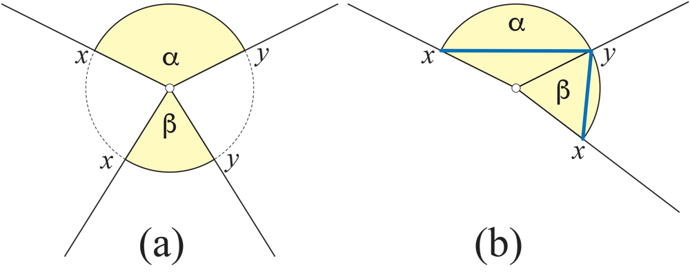
Figure 13.1: (a) ${\alpha}>{\beta}$. (b) $|xy|$ is shorter through angle ${\beta}$ than through ${\alpha}$.

An open convex set may have several vertices as boundary components, as we will see in Example 13.11 below, and at most two convex curves as boundary components, as will be evident in the next result and its proof.

Lemma 13.8 (Simply-connected or cylinder).

Let $S\neq P$ be a closed convex subset of $P$. Then either $S$ is simply-connected, or it is isometric to a cylinder without lids.

Recall from Chapter 9 (Section 9.2.1) that in our usage, simply-connectedness does not assume path-connectedness. However, all convex sets are path-connected.

Proof.

If $S$ has empty interior, the conclusion follows from Lemma 13.2; so we may assume in the following that $S$ has interior points.

The convexity of $S$ implies that each component of $\partial S$ is a simple closed curve, and since it is locally convex by Lemma 13.6, it is a convex curve.

Let $C_{1},C_{2}$ be two components of $\partial S$. There are two possibilities: without loss of generality, $C_{2}$ is nested inside $C_{1}$, or they are not nested. This latter case violates convexity, because a geodesic segment connecting a point inside $C_{1}$ to a point inside $C_{2}$ would necessarily include points exterior to both. So let $C_{2}$ be nested inside $C_{1}$.

The Gauss-Bonnet Theorem implies that the total curvature inside $C_{1}$ is $\leq 2\pi$, and similarly for $C_{2}$. So the total curvature outside $C_{1}$, and also outside $C_{2}$, is $\geq 2\pi$. But the exterior of $C_{2}$ is strictly inside $C_{1}$, and the exterior of $C_{1}$ is strictly inside $C_{2}$. Therefore, either the region between $C_{1}$ and $C_{2}$ has zero curvature, and therefore it is isometric to a cylinder without lids, or at least one the above inequalities is strict and we get a contradiction, establishing the conclusion. ∎

Lemma 13.9 (Vertex point-hole).

Let $S\subset P$ be a convex set and $v$ a vertex in $S$. Then $S\setminus\{v\}$ is convex.

Proof.

The case $S=\{v\}$ is clear, because we consider the empty set to be a convex set.

Consider distinct points $x,y\in S$, and a geodesic segment ${\gamma}$ between them, hence ${\gamma}\subset S$. If $v\not\in\{x,y\}$, ${\gamma}\subset S\setminus\{v\}$, because no geodesic segment will pass through a vertex.

Assume now that $x=v$. Then each point of ${\gamma}\setminus\{v\}$ is inside a geodesic subsegment of ${\gamma}$, hence included in $S\setminus\{v\}$. ∎

Example 13.10.

An example illustrating the cylinder claim of the Lemma 13.8 is provided by $P$ a tall rectangular block, and $S$ the region between two parallel simple closed geodesics close to the middle of the block. Then $S$ is a closed convex set.

Example 13.11.

Lemma 13.8 does not hold for arbitrary convex sets with interior points. Indeed, the set $P\setminus V$ is convex (see Lemma 13.9), open, but not simply-connected.

Example 13.12.

More generally, let $S$ be a simply-connected convex set, and $v$ a vertex interior to $S$. Then $S\setminus\{v\}$ is convex, but not simply-connected. However, the closure of $S\setminus\{v\}$ is convex and simply-connected.

Example 13.13.

A particular instance of Helly’s Theorem states the following: let $S_{1},...,S_{n}$ be a finite collection of convex subsets of ${\mathbb{R}^{2}}$, with $n>3$. If the intersection of every $h=3$ such sets is nonempty, then the whole collection has a nonempty intersection.

The simple example of the four faces of a tetrahedron, each face a closed, convex set, shows that no analogous result holds in our framework.

A more elaborated example places the tetrahedron over a tall right triangular prism. There, the union of the tetrahedron’s lateral faces, minus the top vertex, is a convex set. That set, together with the lateral faces, provides another counterexample.

It remains for future work to consider the above Helly-like problem for $h\geq 4$: Open Problem 18.13.

Lemma 13.14 ($S\supseteq Q$).

If the interior of the closed convex set $S$ contains a simple closed quasigeodesic $Q$, then either $\partial S$ determines with $Q$ a topologically closed cylinder, or $S=P$.

Proof.

Assume the simple closed quasigeodesic $Q$ is included in $S$.

If $Q$ parallels $\partial S$ (in the sense that they bound a cylinder) then $\partial S$ is itself a simple closed quasigeodesic. Assume this is not the case.

Because $Q$ is interior to $S$, the sum of curvatures of vertices inside or on $Q$ is at least $2\pi$. If $\partial S\neq\varnothing$ then, since it is convex towards $S$, the total curvature of the interior of $S$ is $<2\pi$, by Lemmas 13.8 and 13.6, which violates the Gauss-Bonnet Theorem. ∎

We don’t know if every closed convex set is either included in a half-surface bounded by a simple closed quasigeodesic, or is the whole surface. This is not settled by the previous lemma because there $Q$ is interior to $S$. This question is Open Problem 18.11. However, the proof of the previous lemma does show that no closed convex set can strictly enclose more than $2\pi$ curvature. This picture will be completed by Proposition 13.27 and Theorem 13.32 below.

13.4 Geodesic Segments and Convex Sets

In this section we clarify the behaviour of geosegs between points in, or on the boundary of, or outside of, a convex set. The first part of the next result will be particularly useful later.

Lemma 13.15 (Segment vs. convex set).

Let $S\subset P$ be a convex, $S\neq P$.

(i) If $x,y$ are interior points of $S$ and ${\gamma}$ a geodesic segment joining them, then ${\gamma}$ is interior to $S$ (i.e., it does not intersect $\partial S$).

In particular, adding a boundary point to an open convex set yields a convex set.

(ii) If $x$ is an interior point of $S$ and $y\in\partial S$, then all geodesic segments from $x$ to $y$ are interior to $S$, possibly excepting at their extremity $y$.

(iii) If $x,y\in\partial S$ then there is a geodesic segment between them included in the closure $\bar{S}=S\cup\partial S$ of $S$, possibly excepting its extremities $x,y$. Other geodesic segments from $x$ to $y$ might not be included in $\bar{S}$.

In particular, adding two boundary points to an open convex set does not necessarily yield a convex set.

(iv) If $x\in\partial S$ is not by itself a connected component of $\partial S$, then there exists a geodesic segment starting at $x$ and exterior to $S$.

Proof.

(i) Let $B_{1},B_{2}$ be open intrinsic balls around $v_{1},v_{2}$ respectively, with $B_{1}\cup B_{2}\subset S$.

Let $N_{\gamma}\subset P$ be a tubular neighborhood of the image set of ${\gamma}$. View $N_{\gamma}$ as created by translations of ${\gamma}$ sufficiently small so that $N_{\gamma}$ is included in $B_{i}$ around $v_{i}$, $i=1,2$, and so that $N_{\gamma}$ is an open set included in $S$. $N_{\gamma}$ is flat everywhere, except at $v_{1},v_{2}$. Because ${\gamma}$ is strictly inside $N_{\gamma}$, ${\gamma}$ does not intersect $\partial S$.

This claim can also be established by assuming that some geodesic segment between interior points touches $\partial S$, and applying Lemma 13.5 to obtain a contradiction.

(ii) Assume there exists a geodesic segment ${\gamma}$ from $x$ to $y$ that goes outside $S$, so there is a boundary point $z\in\partial S$ on ${\gamma}$ between $x$ and $y$. Assume, moreover, that $z$ is closest to $y$ with these properties.

Notice that such a $z$ exists, i.e., is at positive distance to $y$. To see this, consider a small ball $B_{y}$ around $y$ which contains no vertex of $P$. Then $S\cap B_{y}$ is a convex set in the plane (if $y$ is not a vertex of $P$) or on a cone (if $y$ is a vertex), by Lemma 13.5. Denote by ${\gamma}_{z}$ the sub-arc of ${\gamma}$ from $z$ to $y$. The boundary of this small convex set $\partial(S\cap B_{y})$ is a convex curve, and the image of ${\gamma}_{z}$ is a segment, with the two intersecting in at most two points (because a segment can intersect a convex curve at most twice). This shows $z$ exists as described.

Denote by $A_{z}$ the component of $\partial S$ between $z$ and $y$ such that no point of $S$ is inside the lune $L$ bounded by $A_{z}$ and ${\gamma}_{z}$. $L$ is then bound by a curve $A_{z}$ concave towards $L$ and a straight segment ${\gamma}_{z}$ exterior to $A_{z}$. The Gauss-Bonnet Theorem implies this is only possible if $L$ contained negative curvature, a contradiction.

(iii) Because $x,y\in\partial S$, there exist a sequence of points $x_{n},y_{n}\in S$ such that $x_{n}\to x$, $y_{n}\to y$. Let ${\gamma}_{n}$ be a geodesic segment joining $x_{n}$ to $y_{n}$, $n\in{\mathbb{N}}$. Then there exists a subsequence of $\{{\gamma}_{n}\}_{n}$, which converges to a geodesic segment ${\gamma}$ between $x$ and $y$. Since all ${\gamma}_{n}$ are in $S$, their limit is in $\bar{S}$.

(iv) This claim can be obtained from Lemma 13.5. An alternative proof follows.

The space of unit tangent directions $T_{x}$ at $x$ is a circle, of course of arc-length $\leq 2\pi$.

Assume, in contradiction to the claim that, for any $\nu\in T_{x}$, the maximal geodesic segment ${\gamma}^{\nu}$ starting at $x$ in direction $\nu$ intersects $S\cap B_{x}$, i.e., it has an initial portion of ${\gamma}^{\nu}$ is inside $S$. Choose three directions $\nu_{i}\in T_{x}$, $i=1,2,3$, with the angle between adjacent pairs $\nu_{i},\nu_{j}$ less than $\pi$. With points $x_{i}\in S$ on ${\gamma}^{\nu_{i}}$, the three flat triangles $xx_{i}x_{j}$ are in $S$, and their union forms an open set around $x$, contradicting $x\in\partial S$. ∎

Example 13.4 can be easily elaborated to illustrate all the claims of the above lemma.

Corollary 13.16.

It follows directly from (i) in Lemma 13.15 that the interior of a convex set is still convex.

Lemma 13.17 (Supporting angle).

Let $S\neq P$ be a closed convex subset of $P$ with interior points, and $x$ a boundary point of $S$. There exists tangent directions $\mu,\nu\in T_{x}$ at $x$ of angle $\theta=\theta(\mu,\nu)\leq\pi$ toward $S$, such that:

(i) the geodesic segments ${\gamma}^{\mu}$ and ${\gamma}^{\nu}$ in the directions $\mu,\nu$ do not intersect the interior of $S$, locally; and

(ii) for each $\tau\in T_{x}$ inside $\theta$, the geodesic segment ${\gamma}^{\tau}$ in the direction $\tau$ does intersect the interior of $S$, locally. Here, $\theta$ is regarded as a subarc of $T_{x}$.

Proof.

This can established from Lemma 13.5. An alternative way to prove the claims follows.

Let $B_{x}$ be a small ball around $x$ which contains no vertex of $P$.

Lemma 13.15 shows that there exists a geodesic segment ${\gamma}_{z}$ connecting $x$ to a point $z\in P\setminus S$. Because $P\setminus S\neq\varnothing$ is an open set, there are other points in the neighborhood of $z$ similarly connected to $x$ by geodesic segments that do not intersect the interior of $S$. Denote by $A_{x}$ the maximal open subarc of $T_{x}$ determined by directions of such geodesic segments ${\gamma}_{z}$. Let $\mu,\nu\in T_{x}$ be the extremities of $A_{x}$.

The convexity of $S$ implies that for all $\tau\in A_{x}$, the geodesic segment ${\gamma}^{\tau}$ does not intersect $S\cap B_{x}$. Moreover, $A_{x}\geq\pi$. This establishes claim (i).

The convexity also implies that $\theta=T_{x}\setminus A_{x}\leq\pi$ has the opposite property: for each $\tau\in T_{x}$ inside $\theta$, the geodesic segment ${\gamma}^{\tau}$ intersects the interior of $S\cap B_{x}$. This establishes Claim (ii). ∎

13.5 Relative Convexity

For the next result (Lemma 13.18), we need to modify the notion of convexity to relative convexity, a variation on a notion of relative convexity we employed in [OV14].

Let $S\subset P$ be a contractible closed convex set with interior points. We proved in the previous section that $S$ is bounded by a closed convex curve $C=\partial S$. We glue to $C$ a tall cylinder $L$ with a base but without a top. This satisfies AGT, because a point $p\in C$ is convex to the $S$-side and has angle $\pi$ on the cylinder rim.

Denote by $P^{\#}$ the resulting convex surface. AGT implies that $P^{\#}$ is a polyhedron if and only if $\partial S$ is a geodesic polygon on $P$. Call $S$ relatively convex if its image (also denoted by $S$) is convex on $P^{\#}$.

Note that $C$ is a quasigeodesic on $P^{\#}$.

There are two considerations that lead us to introduce relative convexity in this section, and the relative convex hull ${\rm{rconv}}(S)$ in Section 13.6. First, the failure of vertex-merging to preserve convexity, Example 13.19 below. Second, the failure of the convex hull of points inside a simple closed quasigeodesic $Q$ to remain inside $Q$, Example 13.30 below.

In Section 13.9 we shall use a construction similar to the above, but with respect to simple closed quasigeodesics $Q$ instead of convex curves $C$. The purpose there is to construct the relative convex hull, starting from a non-convex set inside $Q$. So the term “relative” will refer to either construction, depending on the context, and without confusion.

Lemma 13.18 (Vertex merging).

Let $v_{1},v_{2}$ be two vertices interior to the convex set $S\subset P$. Merging $v_{1}$ and $v_{2}$ produces a new polyhedron $P^{\prime}$ and a set $S^{\prime}\subset P^{\prime}$ obtained as the union of $S$ with the two merge triangles $T$. Then $S^{\prime}$ is relatively convex on $P^{\prime}$.

Before we prove this lemma, we show that it is false for convexity, without the “relatively” modifier.

Example 13.19 (doubly-covered quadrilateral).

Figure 13.2 shows an example $S\subset P$ where the insertion of merge triangles causes some geodesic segments in the new set $S^{\prime}$ to leave $S^{\prime}$, violating convexity. In (a), geodesic segments from any point $x$ on the front face to its image $x^{\prime}$ on the back face stay within $S$, whereas after the $v_{1},v_{2}$ merge (b), there are points $x$ whose shortest path to its back-face image $x^{\prime}$ crosses $ab$ outside of $S^{\prime}$.

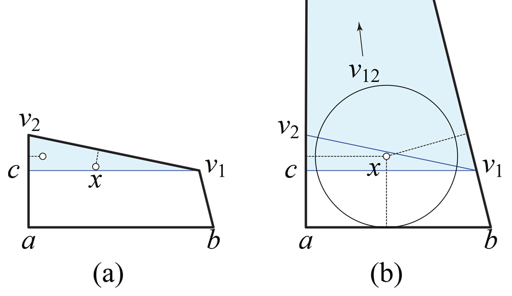
Figure 13.2: (a) $P$ is the doubly-covered quadrilateral $abv_{1}v_{2}$. Convex set $S\subset P$ is the two-sided triangle $cv_{1}v_{2}$, shaded. (b) Merging $v_{1}$ and $v_{2}$ yields $v_{12}$ far above $P$. The resulting set $S^{\prime}$ is $cv_{1}v_{12}$.

Proof.

We know by Lemma 13.15 that the insertion of the triangles $T$ has not affected the boundary of $S^{\prime}$: $\partial S^{\prime}=\partial S=C$, where $C$ is a convex curve. In $P^{\prime\#}$, denote by $L$ the sides of the cylinder glued to $C$. When $L$ is unfolded flat, it forms a rectangle $R$.

Let $x,y\in S^{\prime}$ be two points in $S^{\prime}$, and ${\gamma}$ a geodesic segment between them. We argue that ${\gamma}$ cannot cross $C$. Suppose ${\gamma}$ properly enters $R$ at $x^{\prime}$ and exits at $y^{\prime}$. Then the segment $x^{\prime}y^{\prime}$ along the top of $R$ is shorter, a contradiction to the assumption that ${\gamma}$ is a geodesic segment.

Therefore, $S^{\prime}$ is convex on $P^{\prime\#}$, i.e., $S^{\prime}$ is relatively convex. ∎

13.6 Convex Hull

We mentioned earlier (Section 13.2) that one reason we are not using metrical convexity is that it leads to an unsatisfactory notion of a convex hull. Here we explore the convex hull, and conclude that we need a variation for our purposes in the next chapter.

In analogy with the Euclidean case, define the convex hull ${\rm conv}(S)$ of an arbitrary set $S\subseteq P$ as the intersection of all the convex sets that enclose $S$ on $P$. So, in a familiar sense, it is the smallest convex set with this property.

In the plane, the convex hull of $S$ can equivalently be defined as the set enclosed by a minimal length curve enclosing $S$. However, as we will show in Section 14.3, the two notions do not coincide in our context. Here we focus on the intersection definition.

Example 13.20.

The convex hull ${\rm conv}(V)$ of the vertices $V$ of a doubly-covered triangle $\Delta$ is the whole surface $\Delta$. Similarly, the convex hull of all the vertices of any convex polyhedron $P$ is $P$ itself: ${\rm conv}(V)=P$.

Example 13.21.

In contrast to the Euclidean situation, for $S=P\setminus V$ we have ${\rm conv}(S)=S$, by Lemma 13.9, because $P$ is itself convex, i.e., the vertex holes are not filled-in by the convex hull operation.

Example 13.22.

A particular instance of Radon’s Theorem on (extrinsically) convex sets states that any set of $r=4$ points in ${\mathbb{R}^{2}}$ can be partitioned into two sets whose convex hulls intersect.

The simple example of a tetrahedron shows that no analoguos result holds in our framework. Indeed, the convex hull of any two vertices is the corresponding edge, so any $2:2$ partion of the vertices provides disjoint convex hulls. And the convex hull of any three vertices is the corresponding face, so any $3:1$ partion of the vertices also provides disjoint convex hulls.

If, as in Example 13.13, we again place the tetrahedron over a tall right triangular prism, then the convex hull of the tetrahedron base vertices is the “roof” minus the fourth vertex.

It remains for future work to study the Radon problem for $r\geq 5$, possibly considering closures of convex hulls:

Also worth studying seems to be the existence of a Carathéodory type theorem in our framework. These questions form Open Problem 18.13.

The following two properties follow immediately from the definition of ${\rm conv}(S)$.

Lemma 13.23.

For every $S\subset P$, ${\rm conv}({\rm conv}(S))={\rm conv}(S)$.

For every two sets $S,S^{\prime}\subset P$ with $S^{\prime}\subset S$, ${\rm conv}(S)^{\prime}\subseteq{\rm conv}(S)$.

The next result is particularly useful for computing the convex hull of finite sets.

Lemma 13.24.

For every pair of subsets $S,T$ of $P$ with $T\subset S$, the following holds:

$${\rm conv}(S)={\rm conv}\left(\left({\rm conv}(S\setminus T)\right)\cup T\right).$$

In words: If $S$ is partitioned into two parts, $T$ and $S\setminus T$, then the hull of $S$ is the hull of the union of $T$ with the hull of $S\setminus T$.

Proof.

The set ${\rm conv}\left(\left({\rm conv}(S\setminus T)\right)\cup T\right)$ is convex and includes $S$, hence it also includes ${\rm conv}(S)$.

On the other hand, the convex set ${\rm conv}(S)$ includes ${\rm conv}(S\setminus T)$, by Lemma 13.23, and also includes $T$. Hence it includes ${\rm conv}\left(\left({\rm conv}(S\setminus T)\right)\cup T\right)$ as well. ∎

The next simple result follows from Lemma 13.15.

Lemma 13.25.

The convex hull of every open set is open.

Example 13.26.

Let $\Box$ be a doubly-covered square with vertices $a,b,c,d$, and let $S=\{a,b,c\}\subset\Box$. Then $S$ is closed and, as we prove below, ${\rm conv}(S)=\Box\setminus\{d\}$, hence ${\rm conv}(S)$ is not closed. Refer to Fig. 13.3.

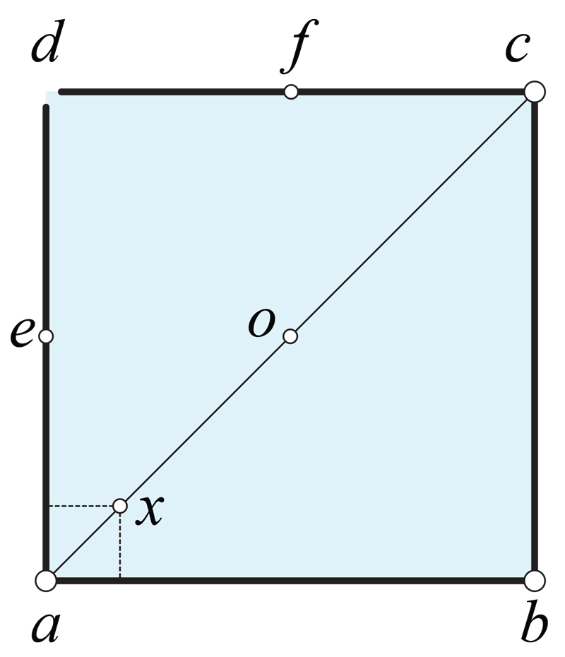
Figure 13.3: ${\rm conv}(\{a,b,c\})$ is $\Box\setminus\{d\}$.

Clearly, ${\rm conv}(S)$ contains the two triangles $abc$, hence also the simple closed quasigeodesic $Q$ determined by the diagonals $ac$. Let $x\in Q$ be a point close to $a$ on the front side, and $x^{\prime}$ its corresponding point on the back side. Then there are two geodesic segments between $x$ and $x^{\prime}$, one “horizontal” and another one “vertical”—parallel to $ab$ and $bc$ respectively. Therefore, there are points of ${\rm conv}(S)$ on the edge $ad$, close to $a$. Moving $x$ continuously towards the center $o$ of $\Box$, shows that the half-edge $ae$ is included in ${\rm conv}(S)$, where $e$ is the midpoint of $ad$. Similarly, ${\rm conv}(S)$ contains the half-edge $cf$, where $f$ is the midpoint of $cd$. Iterating this process establishes that ${\rm conv}(S)$ contains halves of the segments $ed$ and $fd$, and so on. Therefore ${\rm conv}(S)$ contains the whole edges $cd$ and $ad$, except missing the corner point $d$.

The next result will be useful for proving the last statement in Theorem 13.32.

Proposition 13.27 (Dense hull).

Let $S\subset P$ be a closed convex set with interior points, enclosing strictly less than $2\pi$ curvature. Then the convex hull of its complement $S^{\prime}=P\setminus S$ is dense in $P$, and the convex hull of $\partial S$ is dense in $S$.

Proof.

By Lemma 13.25, ${\rm conv}(S^{\prime})$ is open. Then, by Lemma 13.6, the boundary of ${\rm conv}(S^{\prime})$ may consist of vertices and convex curves, convex towards ${\rm conv}(S^{\prime})$. If such a boundary curve existed, it would enclose more than $2\pi$ curvature, contradicting the the Gauss-Bonnet Theorem.

For the second claim, notice that ${\rm conv}(\partial S)\subset S$. Moreover, a continuity argument proves that ${\rm conv}(\partial S)$ has interior points. The remainder is analogous to Lemma 13.6, and to the above argument. ∎

Example 13.28.

Example 13.26 (Fig. 13.3) can be adapted to illustrate Proposition 13.27. See Fig. 13.4.

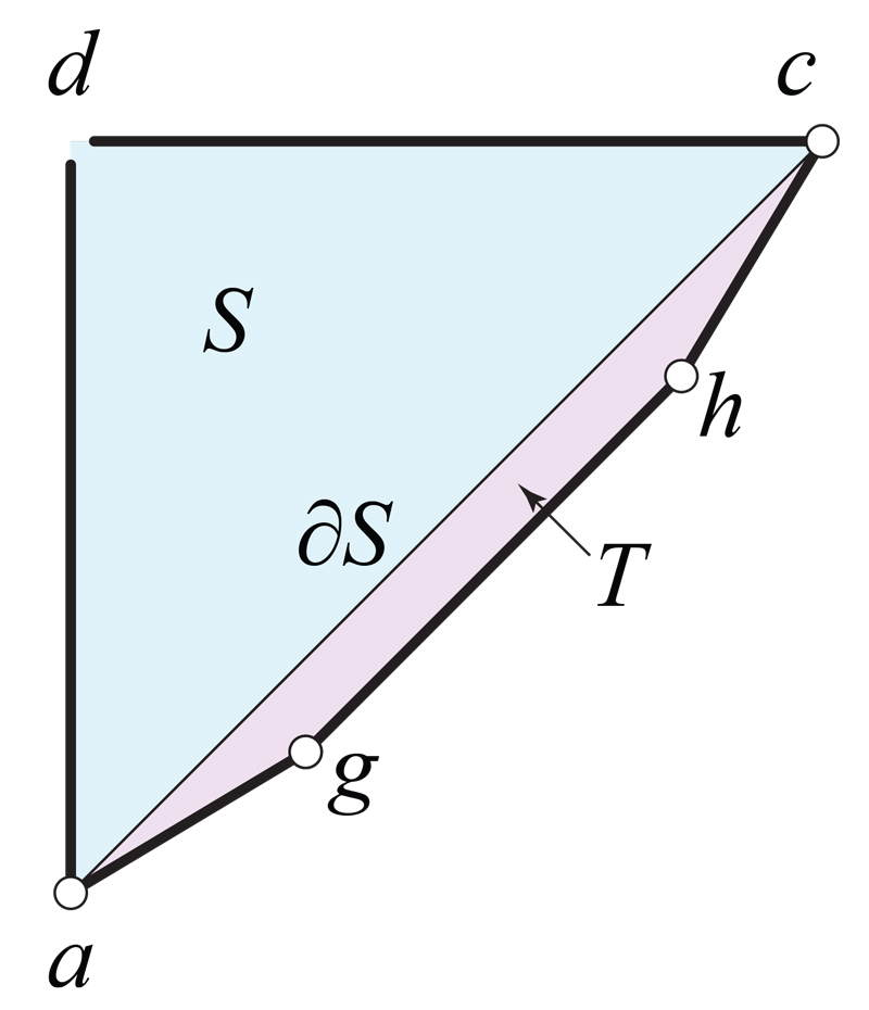
Figure 13.4: ${\rm conv}(\partial S)$ is dense in $S$ and ${\rm conv}(P\setminus S)$ is dense in $P=S\cup T$.

Let $T=ghca$ be an isosceles trapezoid with $gh||ac$, $|g-h|<|a-c|$, and the base angle at $g$ almost $\pi$. Construct, outside $T$, an isosceles right triangle $S=acd$, with $|a-d|=|c-d|$. Let $P$ denote the doubly-covered pentagon $T\cup S$.

The (two-sided) subset $S$ of $P$ is convex, and $\partial S$ consists of the two geodesic segments $ac$. As in the proof of Example 13.26, ${\rm conv}(\partial S)=S\setminus\{d\}$ is dense in $S$, and therefore ${\rm conv}(P\setminus S)=P\setminus\{d\}$ is dense in $P$.

These examples show that the convex hull has some desirable properties, but, for our purposes, some undesirable properties. The doubly-covered square (Example 13.26) shows that ${\rm conv}(V)$ for $V$ a subset of vertices of $P$ could be a set with point holes—so the convex hull of a closed set can be an open set. And in the next section we will show that ${\rm conv}(S)$ for a set $S$ is not always the convex hull of the extreme points of $S$. These considerations lead us to use the notion of relative convexity as first introduced in Section 13.5 above, and the relative convex hull ${\rm{rconv}}(S)$, which will be developed in Section 13.9 below.

Example 13.29.

Let $B_{h}$ be a rectangular box of height $h$, and $Q$ a simple closed geodesic on $B$ parallel to its top and bottom faces, at height $h/2$. If $h$ is large enough then $Q$ is itself a convex set, and ${\rm conv}(Q)=Q$; see Lemma 13.37 and its proof for details. However, for small $h$, $Q$ is not a convex set, and ${\rm conv}(Q)=B$. This shows that the convex hull of a set $S$ is sensitive to the surface of $P$ outside of $S$, and justifies the next section.

13.7 Relative Convex Hull

The phenomena illustrated in the previous examples lead us to a new notion.

By “relative convex hull” ${\rm{rconv}}(S)$ we mean the intersection of all relative convex sets containing $S$, with relative convexity as previously defined in Section 13.5. We will further explore this notion in Section 13.9 below.

Example 13.30 (Pyramid).

Let $P$ be a pyramid, the top of a regular octahedron. In Fig. 13.5(a), both $C_{1}$ and $C_{2}$ are ${\alpha}{\beta}$-convex curves. The convex hull of the corners of $C_{1}$, is the surface above $C_{1}$, including the apex $v_{5}$. However, the convex hull of the corners of $C_{2}=(v_{1},v_{2},v_{3},v_{4})$ is not the surface above $C_{2}$, but instead all of $P$. This is because there are geodesic segments that cross the square base. For example, the shortest path between the midpoints of consecutive edges of $C_{2}$ traverse the square base. Fig. 13.5(b) shows the construction of $P^{\#}$ for $C_{2}$. Then ${\rm{rconv}}(C_{2})$ is the surface above $C_{2}$, because no shortest paths will enter the cylinder inserted below $C_{2}$.

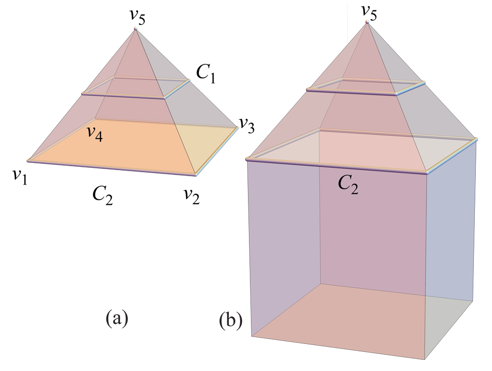
Figure 13.5: (a) ${\rm conv}(C_{1})$ is the pyramid top, but ${\rm conv}(C_{2})=P$. (b) $P^{\#}$ for $C_{2}$.

Example 13.31.

With the following example, we show that:

• neither a digon nor a triangle is necessarily convex;

• Neither ${\rm conv}(V)$ nor ${\rm{rconv}}(V)$ is necessarily closed, for $V$ the set of all vertices inside a simple closed quasigeodesic;

• the exceptional case in Theorem 13.32 below may well appear for the closure of ${\rm{rconv}}(V)$, which in our case is convex but not the convex hull of its extreme points.

Start with the double of the quadrilateral $D=abcd$, where $Q=aba$ is a simple closed quasigeodesic. See Figure 13.6. We could insert rectangles below $Q$, so that everything happens above $Q$.

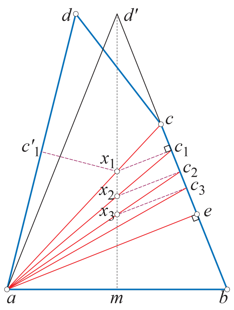
Figure 13.6: $V=\{a,c,d\}$, $\partial\,{\rm{rconv}}(V)=aea$, but $ae\setminus\{a\}\not\in{\rm{rconv}}(V)$.

The construction of $D$ follows: start with an arbitrary line-segment $ab$, and denote by $m$ the mid-point of $ab$. Consider an isosceles triangle $d^{\prime}ab$, and a point $d$ slightly to the left of $d^{\prime}$. Take $c$ on $d^{\prime}b$.

Consider, moreover, $ae$ perpendicular to $d^{\prime}b$, with $e$ on $d^{\prime}b$.

Put $V=\{a,c,d\}$. Then ${\rm{rconv}}(V)$ is the half-surface bounded by the two segments $ae$, without those segments (but including $a$). To see this, let $x_{1}$ be the intersection point between $ac$ and $d^{\prime}m$, and $c_{1}$ the foot of $x_{1}$ onto $d^{\prime}b$. Then the geodesic segment from $x_{1}$ to its “opposite” point goes through $c_{1}$, by construction. So $c_{1}$ belongs to ${\rm{rconv}}(V)$, and therefore $ac_{1}$ is included in ${\rm{rconv}}(V)$. (Notice that $|x_{1}-c_{1}|<|x_{1}-c_{1}^{\prime}|$.)

Now let $x_{2}$ be the intersection point between $ac_{1}$ and $d^{\prime}e$, and $c_{2}$ the foot of $x_{2}$ onto $d^{\prime}b$. Then the geodesic segment from $x_{2}$ to its “opposite” point goes through $c_{2}$, by construction. So $c_{2}$ belongs to ${\rm{rconv}}(V)$, and therefore $ac_{2}$ is included in ${\rm{rconv}}(V)$.

Iterate, and pass to the limit.

It follows (as one can prove by running the above procedure backward) that all points above $ae$ belong to ${\rm{rconv}}(V)$, but not $ae$ (see Lemma 13.36).

Clearly, the digon $aca$ is not convex. Also, consider that if we “split” the vertex $a$ into vertices $a^{\prime},a^{\prime\prime}$, then neither is the triangle $a^{\prime}a^{\prime\prime}c$ convex.

13.8 Extreme Points

An extreme point of a convex set $S\subseteq P$ is a point in $S$ that is not interior to any geodesic segment joining two points of $S$. For example, every vertex is an extreme point for every convex set containing it.

Roughly, the Krein–Milman Theorem states that every compact convex set is the extrinsic convex hull of its extreme points. The closest analogy for ag-convexity we could prove is the following theorem, which will be invoked later.

Theorem 13.32.

Let $S$ be a closed convex subset of $P$ with $\partial S$ a closed curve, enclosing strictly less than $2\pi$ total curvature. Then either $S$ is the relative convex hull of its extreme points, or $\partial S$ contains a geodesic arc which is not a geodesic segment. In the former case, the interior extreme points of $S$ are all vertices.

We do not know if the above theorem statement is still true without the “relative” modifier; Open Problem 18.12.

Proof.

Case 1. If $S\subset P$ has empty interior then the conclusion follows from Lemma 13.2, which shows that $S$ is either a point, a geodesic arc, or a simple closed geodesic.

Case 2. Assume $S\subset P$ has non-empty interior. The proof proceeds by induction over the number of vertices of $P$ interior to $S$.

For the base case, assume $S$ has exactly one interior vertex $v$. By Lemma 13.6, $\partial S$ is locally isometric to a planar convex curve. If $\partial S$ contains a geodesic arc which is not a geodesic segment, we have established the lemma claim.

So assume now that $\partial S$ contains a geodesic segment, maximal with respect to inclusion, between its corners $v_{i}$, $v_{i+1}$. Then we get a geodesic-segment triangle $vv_{i}v_{i+1}$, which is the convex hull of its extreme points. This is valid for all such geodesic-segment arcs in $\partial S$.

If $\partial S$ contains an arc $A$ locally isometric to a planar strictly convex curve, then each point of $A$ is an extreme point, and the conclusion follows.

For the general case, again if $\partial S$ contains a geodesic arc that is not a geodesic segment, we are finished. So now we prove that $S$ is the relative convex hull of its extreme points.

Assume that $S$ has at least two interior vertices, say $v_{1}$ and $v_{2}$. Because they are inside $Q$, ${\omega}_{1}+{\omega}_{2}<2\pi$. Let ${\gamma}$ be a geodesic segment joining them in $S$.

Merge $v_{1}$ and $v_{2}$ to $v_{12}$ along ${\gamma}$ to obtain a new surface $P^{\prime}$, hence where $P^{\prime}$ is $P$ cut open along ${\gamma}$ and the union $T$ of two twin triangles is inserted. The set $S$ with $T$ inserted yields $S^{\prime}$, a relatively convex set of $P^{\prime}$ (Lemma 13.18).

Because $\partial S^{\prime}=\partial S$ by Lemma 13.15, $S^{\prime}$ is closed, because $S$ is closed.

By the induction hypotheses, $S^{\prime}$ is the relative convex hull of its extreme points $E^{\prime}$ on $P^{\prime\#}$. Clearly, the only extreme point of $S^{\prime}$ in $T$ is $v_{12}$. Put $E^{\prime\prime}=E^{\prime}\setminus\{v_{12}\}$ and, on $P$, $E=E^{\prime\prime}\cup\{v_{1},v_{2}\}$. It suffices to show that (i) $E$ is the set of extreme points of $S$, and (ii) $S={\rm conv}(E)$.

(i) Since $E^{\prime\prime}$ is included in the part of $S^{\prime}$ isometric to $S$, each point in $E^{\prime\prime}$ in also extreme for $S$, as are the vertices $v_{1}$, $v_{2}$.

(ii) One can easily see that each convex set on $P^{\prime}$ containing $E^{\prime}$ corresponds, via digon-tailoring $T$, to a convex set on $P$ containing $E$, and conversely. So the intersection of all such sets on $P^{\prime}$ corresponds to the intersection of their correspondents on $P$, and conversely. Consequently, $S={\rm{rconv}}(E)$.

The last claim of the theorem—that the interior extreme points of $S$ are all vertices—follows from Proposition 13.27 and its proof. ∎

Note that throughout the induction, the boundary of all the sets remains fixed at $\partial S$.

The next example illustrates the exceptional situation of Theorem 13.32.

Example 13.33 (Extreme Points).

Consider a “tall” triangular prism with top $abc$ and base $a^{\prime}b^{\prime}c^{\prime}$. Now add a point $v$ on the line containing $bb^{\prime}$, above $b$, and let $P$ be the boundary of the extrinsic convex hull of $\{a^{\prime},b^{\prime},c^{\prime},a,c,v\}$. See Fig. 13.7. Then $Q=abc$ is a simple closed quasigeodesic and the “roof” above $Q$—all the surface of $P$ above $Q$—is our convex set. (Here we need the prism to be sufficiently tall, but for clarity the figure is more squat.) Take points $x,y\in P$ with $x$ on $ab$ close to $a$ and $y$ on $bc$ close to $c$. Then the arc of $Q$ from $x$ to $y$ through $b$ is not a geodesic segment.

Note that $b$ is not an extreme point of $S$, because $b$ is interior to geodesic segments connecting points on $ab$ and $bc$ that are close to $b$. The only extreme points of $S$ are $a$, $c$ and $v$, and so $S$ is not the convex hull of its extreme points. This is the exception in Theorem 13.32.

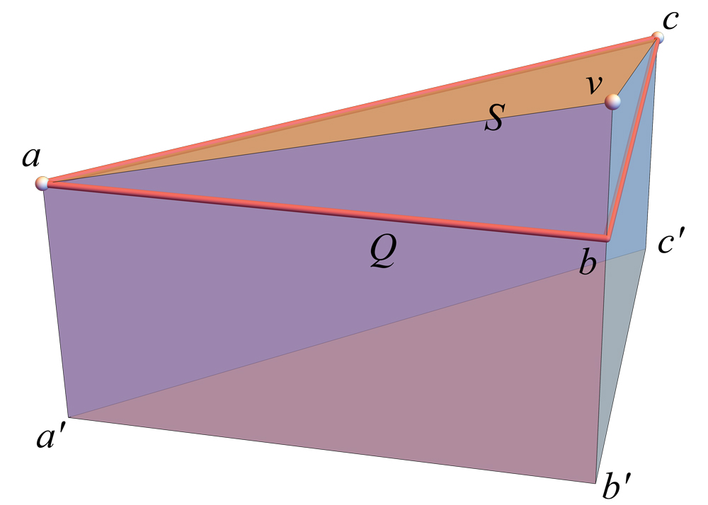
Figure 13.7: The region above the simple closed quasigeodesic $Q$ is convex, but is not the convex hull of its extreme points $a,c,v$.

Example 13.34 (Simple closed geodesic).

For the simple closed geodesic $Q$ on $B_{h}$, the rectangular box of height $h$ considered in Example 13.29, ${\rm conv}(Q)=Q$ holds, and there are no extreme points on $Q$.

Denote by ${\rm{ext}}(S)$ the extreme points of the convex set $S$.

Lemma 13.35.

For any set $S\subset P$, ${\rm{ext}}({\rm conv}(S))\subset S$.

Notice that not all extreme points of the closure of ${\rm conv}(S)$ are in $S$, as Example 13.26 shows.

Proof.

Assume there exists a point $x$ in ${\rm{ext}}({\rm conv}(S))\setminus S$. Then, since $x$ is not interior to any geodesic segment joining two points of ${\rm conv}(S)$ (because it is extreme), the set ${\rm conv}(S)\setminus\{x\}$ is still convex (see the proof of Lemma 13.9). So we have $S\subset{\rm conv}(S)\setminus\{x\}\subset{\rm conv}(S)$ and ${\rm conv}(S)\setminus\{x\}\neq{\rm conv}(S)$, contradicting the minimality of ${\rm conv}(S)$. ∎

Lemma 13.36.

For any $S\subset P$, if ${\rm conv}(S)$ contains a boundary geoarc which is not a geoseg, then $S$ also contains that arc.

Proof.

Assume the contrary be true, and let $A\subset{\rm conv}(S)$ be a maximal (with respect to inclusion) such geoarc not in $S$. So $A\subset\partial({\rm conv}(S))\setminus S$. Remove $A$ from ${\rm conv}(S)$, but leave its extremities, and denote by $K$ the resulting set. It follows, just as in the proof of Lemma 13.9, that $K$ is a convex set including $S$ and strictly included in ${\rm conv}(S)$, a contradiction to the inclusion-minimality of ${\rm conv}(S)$. ∎

Example 13.31 also illustrates this result. Indeed, in Fig. 13.6, the arc $aea$ is a boundary geoarc of ${\rm{rconv}}(\{a,c,d\}$), but not a geoseg. And that arc is not included in $\{a,c,d\}$, hence neither is it included in ${\rm{rconv}}(\{a,c,d\})$.

13.9 Relative Convex Hull of Vertices

We return to the notion of relative convexity and the relative convex hull, used in the proof of Theorem 13.32. For our purposes we only consider the relative convex hull of vertices $V$ that fall to one side of (i.e., inside, or above) a simple closed quasigeodesic $Q$.

Notation.

1. $Q$ quasigeodesic. Orient $Q$ counterclockwise (ccw), and let $P^{+}$ be the half-surface to the left of (above) $Q$. $P^{\#}$ is $P^{+}$ union the unbounded cylinder to the right of (below) $Q$.

2. $V$: Set of (positive curvature) vertices inside or on $Q$.

3. For $C$ any simple closed curve in $P^{+}$, let $R(C)$ be the region of $P^{+}$ to the left of $C$. So $\partial R(C)=C$. This is well-defined because $C$ is a simple curve. And because it is oriented ccw, $R(C)\subset P^{+}$.

Given $Q$ oriented so that $V$ is to $Q$’s left, define a polyhedron $P^{\#}(Q)=P^{\#}$ as in Section 13.5: Cut $P$ along $Q$ and insert below $Q$ a sufficiently tall cylinder; for example, a cylinder of height equal to $\textrm{diam}(P)$. Because $Q$ is convex to both sides, AGT implies that $P^{\#}$ is a convex polyhedron.

Note that $Q$ is strictly ${\alpha}{\beta}$-convex on $P^{\#}$, because ${\beta}_{i}=\pi$ at all corners of $Q$, and corners have positive curvature.

Now we define the relative convex hull ${\rm{rconv}}(V)=H$ of $V$ to be the intersection of all the convex sets that enclose $V$ on $P^{\#}$. This is the same notion earlier explored in Section 13.7, but here we focus on vertices inside $Q$.

Lemma 13.37.

Let $V$ be a set of points on $P$, inside a simple closed quasigeodesic $Q$. The relative convex hull ${\rm{rconv}}(V)=H$ of $V$ can be obtained from only employing geodesic segments, and consequently convex sets, inside $Q$ (instead of constructing $P^{\#}$).

Proof.

Let $x,y\in H$ be two points in $H$, and ${\gamma}$ a geodesic segment between them. We argue that ${\gamma}$ cannot cross $Q$.

When the cylinder attached below $P^{\#}$ is unfolded flat, it forms a rectangle $R$. Suppose ${\gamma}$ properly enters $R$ at $x^{\prime}$ and exits at $y^{\prime}$. Then the segment $x^{\prime}y^{\prime}$ along the top of $R$ is shorter, a contradiction to our assumption. (Note $x^{\prime}y^{\prime}$ is a portion of $Q$, and it is possible that $H$ shares that portion of $Q$.) ∎

A node $n$ of a geodesic polygon $N$ is a point of $N$ interior to no geodesic subarc of $N$. Call it a g-node if at least one side of $N$ incident to $n$ is not a geoseg (instead a geoarc), and a gs-node otherwise.

Recall that Lemma 13.6 showed that, if $S$ is closed and convex, then $\partial S$ is strictly ${\alpha}{\beta}$-convex; and if $S$ has interior points then $\partial S$ is ${\alpha}{\beta}$-convex but not necessarily strictly. We now explore to what extent there is a converse to this lemma, a result we need to compute ${\rm{rconv}}(S)$.

Lemma 13.38 (${\alpha}{\beta}$ converse).

Let $S$ be a set satisfying these conditions: (1) $S\subset R(Q)$ contains $V$, (2) $\partial S$ is a geodesic polygon, and (3) any geoarcs of $\partial S$ which are not geosegs, are not included in $S$.

Then $S$ is relatively convex if and only if $\partial S$ is strictly ${\alpha}{\beta}$-convex at each gs-node, and ${\alpha}{\beta}$-convex at each g-node.

Proof.

If $S$ is relatively convex, the statement is covered by the ${\alpha}{\beta}$-convexity Lemma 13.6. The remainder of the proof establishes the converse: That if $\partial S$ is ${\alpha}{\beta}$-convex at the gs- and g-nodes as above, then $S$ is relatively convex.

Consider first two boundary points $x,y\in\partial S$ (the roles $x$ and $y$ will play, will be decided later) and let ${\gamma}^{\prime}$ be a geoseg joining them, with ${\gamma}^{\prime}$ not included in $\bar{S}=S\cup\partial S$. We now show that there is a subarc ${\gamma}$ of ${\gamma}^{\prime}$ (possibly ${\gamma}={\gamma}^{\prime})$ that lies completely external to the interior $\mathring{S}$ of $S$.

Notice that ${\gamma}^{\prime}$ intersects $\partial S$ finitely many times. Otherwise, since $\partial S$ is formed by geoarcs, hence locally by geosegs, we could find arcs $A$ of $\partial S$ arbitrarily small, having common extremities with subarcs of ${\gamma}^{\prime}$. But those arcs would be ramifying geosegs, impossible.

Therefore, possibly replacing ${\gamma}^{\prime}$ with a subarc ${\gamma}$, we may assume that ${\gamma}$ lies completely external to the interior $\mathring{S}$ of $S$.

Let $F$ be the region of $P$ bounded by ${\gamma}$ and the arc $\partial^{*}S$ of $\partial S$ from $x$ to $y$, so that $F$ doesn’t include $S$. Then $\mathring{F}$ contains no vertex, by hypothesis.

Now we are going to identify a geoarc $g$ from $x$ to $y$ inside $\bar{S}$. The boundary of $S$ is, in particular, a convex curve, hence we may construct with AGT the double $S^{\#}$ of $\bar{S}$. Let $g$ be a geoseg on $S^{\#}$ from $x$ to $y$. It is included in a half-surface of $S^{\#}$, because geosegs do not branch. So we may assume that $g$ is in $\bar{S}$.

We prove next that $g$ is shorter than or equal to ${\gamma}$: $\ell(g)\leq\ell({\gamma})$. Notice that the cut locus $C(x)$ of $x$ on $S^{\#}$ doesn’t intersect $g$, which is a geoseg on $S^{\#}$. On $S^{\#}$, put $\{c_{1},\ldots,c_{k}\}=C(x)\cap\partial\bar{S}$. Each point $c_{j}$ is the extremity of two digons of $S^{\#}$ at $x$ (one on each copy of $\bar{S}$). Remove all those digons from $\bar{S}\subset S^{\#}$ and zip close the result by AGT. We get a doubly covered flat surface, by Lemma 2.2. Denote by $S^{*}$ the part of it bounded by $\partial^{*}S$ and $g$ which doesn’t include $\partial S$.

We compare now $F$ and $S^{*}$, which are both flat (hence planar) polygons. Clearly, the angles ${\alpha}^{*}$ of $\partial^{*}S$ towards $S^{*}$ are at most $\pi$, and they are smaller or equal to those towards $F$, denoted by ${\beta}^{*}$. (For convenience, we suppress the indices of ${\alpha}^{*}$ and ${\beta}^{*}$.) By the extension of Cauchy’s Arm Lemma (Theorem 2.7). we obtain that $g$ is shorter than or equal to ${\gamma}$.

Next we will consider separately the cases of $x$ or $y$ (or both) belongs to $S$. That case-distinction and the non-strict inequality will imply convexity, via strictness or non-strictness of ${\alpha}{\beta}$-convexity.

Case 1. $x$ and $y$ in $S$. The equality case appears if ${\alpha}^{*}={\beta}^{*}$ everywhere, meaning that $\partial^{*}S$ is outside $S$. So if $x,y\in\partial S\cap S$ the inequality $\ell(g)<\ell({\gamma})$ is strict because of the strictness of ${\alpha}{\beta}$-convexity, hence all geosegs between them are in $S$.

Case 2. Consider now two points $x^{\prime},y^{\prime}\in\mathring{S}$. From these two points we will obtain $x$ and $y$. Assume ${\gamma}^{\prime}$ exits $S$. Because $\partial S$ is a convex curve towards $S$, ${\gamma}^{\prime}$ must intersect it at least two times. Choosing two such points $x,y$, the above argument implies the ramification of ${\gamma}^{\prime}$ assuming $|g|=|{\gamma}|$, hence not strict ${\alpha}{\beta}$-convexity, impossible. So ${\gamma}^{\prime}$ lies inside $\mathring{S}$.

Case 3. The case $x\in\partial S$ and $y^{\prime}\in\mathring{S}$ can be treated analogously, completing the proof. ∎

Example 13.39.

The statement of Lemma 13.38 is not necessarily true if $S$ does not include all of $V$: $V\setminus S\neq\varnothing$.

1. To see this, take the quadrilateral $H=abcd$ formed by three equilateral triangles $obc,ocd,oda$, and let $P^{\prime}$ be the double of $H$. Let $P$ be obtained from $P^{\prime}$ by extending it below by long rectangles. See Figure 13.8(a). $Q=aobo^{\prime}a$ is a simple closed quasigeodesic on $P$ (with $o^{\prime}$ “opposite” to $o$). Let $S=R(oco^{\prime}do)$ be the closed set constituted by $\triangle ocd$ and $\triangle o^{\prime}cd$. Observe that the boundary of $S$ is not strictly ${\alpha}{\beta}$-convex: both the angles ${\alpha}$ and ${\beta}$ at $c$ are $120^{\circ}$ (and similarly at $d$). Then by Lemma 13.6(i), which established that closed $S$ are strictly ${\alpha}{\beta}$-convex, $S$ is not convex. Indeed, there is a geoseg outside $S$ from $x$ to $x^{\prime}$ on the back, for $x$ on $oc$ (and similarly for points on $od$). And for the same reason, there are geosegs from $o$ to $o^{\prime}$ outside $S$, namely $oeo^{\prime}$ and $ofo^{\prime}$.

   

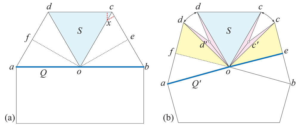
   Figure 13.8: $S$ is not convex. (a) Lemma 13.38 doesn’t apply because $\partial S$ is not strictly ${\alpha}{\beta}$-convex at $c$ and $d$. (b) After insertion of digons, $\partial S$ is strictly ${\alpha}{\beta}$-convex, but Lemma 13.38 does not hold in this case because $S$ doesn’t include $c^{\prime}$ and $d^{\prime}$.

2. Now we show that even altering the example so that every gs-node on $\partial S$ is strictly ${\alpha}{\beta}$-convex, does not always permit the converse conclusion that $S$ is convex. Modify $P$ by inserting two digon doubled triangles along $oc$ and $od$; see Figure 13.8(b). Each triangle has base angles $7.5^{\circ}$, and so adds $15^{\circ}$ to $c$, and $d$, and adds a total of $30^{\circ}$ of angle at $o$. Cut out $30^{\circ}$ at $o$ below $o$, so that $o$ is again flat. Now the $Q$ used above is no longer a quasigeodesic, but $Q^{\prime}=aoeo^{\prime}a$ is a simple closed quasigeodesic. The effect of the digons is two-fold. First, $c$ and $d$ now are both strictly ${\alpha}{\beta}$-convex, and $\partial S$ remains strictly ${\alpha}{\beta}$-convex at $o$ and at $o^{\prime}$. So $S$ is closed, $\partial S$ is a geoseg polygon, strictly ${\alpha}{\beta}$-convex at every gs-node (and it has no g-nodes). So $S$ satisfies all but one condition of Lemma 13.38, which would allow concluding that $S$ is convex. The missing condition is that $V\setminus S\neq\varnothing$: $S$ does not include the two digon vertices—call them $c^{\prime}$ and $d^{\prime}$—which are now part of $V$. And again the geosegs $oeo^{\prime}$ and $ofo^{\prime}$ lie outside of $S$, showing that indeed $S$ is not convex.

3. Next, alter $S$ to include the digon vertices $c^{\prime}$ and $d^{\prime}$: $S^{\prime}=R(oc^{\prime}co^{\prime}dd^{\prime}o)$. So now $V\setminus S=\varnothing$. But $\partial S$ is not ${\alpha}{\beta}$-convex at $c^{\prime}$ and $d^{\prime}$: they both have ${\alpha}={\beta}=165^{\circ}$. So again the preconditions for Lemma 13.38 are not satisfied, and $S^{\prime}$ is not convex.

4. If $S=R(oeo^{\prime}fo)$, then $o$ is a g-node of $\partial S$, which is strictly ${\alpha}{\beta}$-convex at $o$: ${\alpha}=150^{\circ},{\beta}=210^{\circ}$. However, the geoarcs $oeo^{\prime}$ and $o^{\prime}fo$ must not be included in $S$ for Lemma 13.38 to apply. However, $S$ is nevertheless relatively convex.

5. If $S=Q=aoeo^{\prime}a$ in Figure 13.8(b), then $\partial S$ is not strictly ${\alpha}{\beta}$-convex at $o$ (${\alpha}={\beta}=180^{\circ}$), but again the lemma does not apply because $\partial S$ contains the geoarc $oeo^{\prime}$. Again, $S$ is relatively convex.

The next result gathers the proven facts about ${\rm{rconv}}(V)$.

Theorem 13.40 (${\rm{rconv}}(V)$).

Let $V$ be the set of all (at least three) vertices of $P$, inside a simple closed quasigeodesic $Q$. $V$ might also include some, but not all, vertices on $Q$, such that $\sum_{v\in V}{\omega}_{v}<2\pi$.

Then $H={\rm{rconv}}(V)$ is simply-connected and its boundary $\partial H$ is a geodesic polygon, strictly ${\alpha}{\beta}$-convex at gs-nodes and ${\alpha}{\beta}$-convex at g-nodes, on $P^{\#}$. Moreover, ${\rm{ext}}(H)=V$.

It will be established in Theorem 14.12 that $H={\rm{rconv}}(V)$ can be constructed in time $O(n^{5}\log n)$ where $n=|V|$.

Proof.

By Lemma 13.35, ${\rm{ext}}({\rm{rconv}}V)\subset V$, and clearly $V\subset{\rm{rconv}}V$, hence ${\rm{ext}}(H)=V$. Therefore, each point in $\partial\,{\rm{rconv}}(V)\setminus V$ is interior to a geoarc, so $\partial rconv(V)$ is a geodesic polygon. The ${\alpha}{\beta}$-convexity follows now from Lemma 13.38.

The simply-connectedness follows from the algorithmic construction in Section 14.4, justified by Lemma 13.38. ∎

Example 13.41.

Notice that the claim that ${\rm{ext}}(H)=V$ may not hold when $V$ does not include all vertices of $P$ inside $Q$. This can be seen by adapting Example 13.26, Fig. 13.3, as follows.

Imagine there is another vertex $a^{\prime}$ close to $a$, above $a$, and almost flat. (This vertex $a^{\prime}$ is added so that $|V|\geq 3$.) Then, in the upper-left half-surface $S$ bounded by the simple closed quasigeodesic $Q=aca$, take $V=\{a,a^{\prime},c\}$ (i.e., skip one vertex $d$ inside $Q$). Then $H={\rm conv}(V)=S\setminus\{d\}$, by Proposition 13.27. Therefore, $H$ is not simply-connected and $\partial H$ is not a geodesic-segment polygon.

13.10 Summary of Properties

We attempt to succinctly summarize below the facts about convexity established in this chapter, either in lemmas and theorems, or via examples. The goal is to help the reader interested in applications of this theory. Please note that, unless otherwise specified, “convexity” means “ag-convexity.”

Ag-Convexity

1. $S$ closed convex $\implies$ Either point, arc, geodesic, or has interior points. Lemma 13.2.

2. Closure $\bar{S}$ of convex $S$ $\centernot\implies$ $\bar{S}$ convex. Example 13.4.

3. $S$ closed convex $\implies$ $\partial S$ a convex curve, and if a geodesic polygon, then ${\alpha}{\beta}$-convex. Lemma 13.6

4. $S$ closed convex $\implies$ $S$ encloses $\leq 2\pi$ curvature.

5. $S$ closed convex $\implies$ simply-connected, or cylinder. Lemma 13.8.

6. $S$ convex and $v\in S$ a vertex $\implies$ $S\setminus\{v\}$ convex. Lemma 13.9.

7. $S$ convex and not closed $\centernot\implies$ simply-connected. Example 13.12.

8. No Helly type theorem for $h=3$. Example 13.13.

9. $S$ closed convex and includes $Q$ $\implies$ cylinder, or $S=P$. Lemma 13.14.

Geodesic Segments and Convex Sets

1. $S$ convex $\implies$ ${\gamma}$ connecting interior points $x_{1},x_{2}$ does not meet $\partial S$. Lemma 13.15.

2. $S$ convex, $x$ interior to $S$ and $y\in\partial S$ $\implies$ all geodesic segments from $x$ to $y$ are interior to $S$, possibly excepting their extremity $y$. Lemma 13.15.

3. $S$ convex, $x,y\in\partial S$ then there is a geodesic segment between them included in the closure $\bar{S}$ of $S$. Lemma 13.15.

4. $S$ convex; $x\in\partial S$ is not itself a component of $\partial S$ then there exists a geodesic segment starting at $x$ and exterior to $S$. Lemma 13.15.

5. $S$ convex $\implies$ the interior of $S$ is convex. Corollary 13.16.

6. $S\neq P$ convex with interior points, $x\in\partial S$ $\implies$ supporting angle at $x$. Lemma 13.17.

Relative Convexity

1. $S$ convex and $v_{1},v_{2}$ merge $\implies$ $S^{\prime}$ relatively convex. Lemma 13.18.

2. $S$ convex and $v_{1},v_{2}$ merge $\centernot\implies$ $S^{\prime}$ convex. Example 13.19.

Convex Hull Properties: ${\rm conv}(S)$

1. $V$ vertices of $P$ $\implies$ ${\rm conv}(V)=P$. Example 13.20.

2. ${\rm conv}(P\setminus V)=P\setminus V$. Example 13.21.

3. No Radon type theorem for $r=4$. Example 13.22.

4. For $S^{\prime}\subset S$, ${\rm conv}(S^{\prime})\subseteq{\rm conv}(S)$. Lemma 13.23.

5. For $T\subset S$, ${\rm conv}(S)={\rm conv}\left(\left({\rm conv}(S\setminus T)\right)\cup T\right)$. Lemma 13.24.

6. $S$ open $\implies$ ${\rm conv}(S)$ open. Lemma 13.25.

7. $S$ closed $\centernot\implies$ ${\rm conv}(S)$ closed. Example 13.26.

8. $S$ closed, convex, with interior points, enclosing $<2\pi$ curvature $\implies$ ${\rm conv}(P\setminus S)$ dense in $P$, ${\rm conv}(\partial S)$ dense in $S$. Proposition 13.27.

9. For box $B_{h}$ and $Q$: ${\rm conv}(Q)=Q$ or ${\rm conv}(Q)=B$, depending on $h$. Example 13.29.

Relative Convex Hull: ${\rm{rconv}}(S)$

1. Convexity and relative convexity can differ. Example 13.30.

2. Neither a digon nor a triangle is necessarily convex; ${\rm conv}(V)$ is not necessarily closed; the closure of ${\rm{rconv}}(V)$ is not the convex hull of its extreme points. Example 13.31.

Extreme Points: ${\rm{ext}}(S)$

1. $S$ closed convex with $\partial S$ enclosing $<2\pi$ curvature. Either $S={\rm{rconv}}({\rm{ext}}(S))$, or $S$ contains a non-segment geoarc. Theorem 13.32. Exception: Examples 13.31, 13.33.

2. $S$ closed, convex and ${\rm conv}(S)\neq{\rm conv}({\rm{ext}}(S))$. Example 13.33.

3. $S$ closed convex with ${\rm{ext}}(S)=\varnothing$. Example 13.34.

4. ${\rm{ext}}({\rm conv}(S))\subset S$. Lemma 13.35.

   Not all extreme points of the closure of ${\rm conv}(S)$ are in $S$. Example 13.26.

5. $\partial{\rm conv}(S)$ contains a non-segment geoarc only if $S$ does so. Lemma 13.36.

Relative Convex Hull of Vertices

1. $S\subset R(Q)$, points $V$ in $S$: ${\rm{rconv}}(S)$ can be constructed without $P^{\#}$. Lemma 13.37.

2. $S\subset R(Q)$, $V\subset S$, $\partial S$ ${\alpha}{\beta}$-convex $\implies$ $S$ relatively convex. Lemma 13.38.

3. Lemma 13.38 is not true if $V\setminus S\neq\varnothing$. Example 13.39.

4. $V$ all vertices inside $Q$, + some on $Q$ $\implies$ $H={\rm{rconv}}(V)$ simply-connected, $\partial H$ a geodesic polygon, ${\alpha}{\beta}$-convex on $P^{\#}$. ${\rm{ext}}(H)=V$. Theorem 13.40.

5. ${\rm{ext}}(H)\neq V$ if $V$ does not include all vertices inside $Q$. Example 13.41.

Chapter 14 Minimal-length Enclosing Polygon

In this chapter we explore the minimial-perimeter polygon $Z$ enclosing a set of vertices $V$ in or on a quasigeodesic $Q$. We derive its key properties, and provide a polynomial-time algorithm for constructing it (Section 14.2). We then show that this polygon is not always the same as $\partial\,{\rm{rconv}}(V)$ (Example 14.10). The algorithm for $Z$ also works to construct $\partial\,{\rm{rconv}}(V)$ with minor modifications (Section 14.4).

In the next chapter we will show that either of these notions can support an algorithm that ensures that sequential vertex-merging cuts do not disconnect $P^{+}$.

14.1 Properties of the Minimal Enclosing Polygon

Notation.

We repeat some previous notation and introduce new notation to be used subsequently. We again use the abbreviation geoseg to mean “geodesic segment” and geoarc to mean a simple geodesic that may or may not be a geoseg.

1. $Q$ quasigeodesic. Orient $Q$ counterclockwise (ccw), and let $P^{+}$ be the closed half-surface to the left of (above) $Q$. $P^{\#}$ is $P^{+}$ union the unbounded cylinder to the right of (below) $Q$.

2. $V$: Set of (positive curvature) vertices inside or on $Q$.

3. For $C$ any simple closed curve in $P^{+}$, let $R(C)$ be the closed region of $P^{+}$ to the left of $C$ (“R” for region). So $\partial R(C)=C$. This is well-defined because $C$ is a simple curve. And because it is oriented ccw, $R(C)\subset P^{+}$.

4. For $C$ any curve on $P$, $\ell(P)$ denotes its length.

Definition of $\min\ell$.

For a finite set $V$ of points in the plane, ${\rm conv}(V)$ is precisely the set bounded by the minimal length curve enclosing $V$. We adapt this property for vertices $V\subset P^{+}$. Toward that end, we define $Z=Z(V)=\min\ell[V]$ to be the minimal-length geodesic polygon enclosing $V$. Here enclosing is to the left when $Z$ is oriented ccw. We must also stipulate that “enclosing” means that the interior of the region between $Z$ and $Q$ is empty of vertices. Otherwise a clockwise traversal of the boundary of any triangle $\triangle\subset P^{+}$ would enclose $V$ to its left, and in fact would enclose all of $P\setminus\triangle$. Also, for a simple closed geodesic enclosing $V$, its position is not fixed by the above requirements, in the sense that it could be “slid” parallel to itself while remaining a geodesic of the same length. In such a case, we define $Z$ to be “lifted” to a position that touches a vertex.

Each edge of the geodesic polygon $Z$ is a geoarc but not necessarily a geoseg. See, e.g., Fig. 14.2(b). We view polygons, and so $Z$, as the boundary, not the region enclosed, which is denoted by $R(Z)$.

Here we concentrate on properties of $Z$ and algorithms to construct $Z$. We stress that all the following considerations take place on $P^{\#}$ and not on $P$. For simplicity, we will omit in the rest of this section the modifier “relative,” which would refer precisely to $P^{\#}$.

We first establish three basic properties of $Z=Z(V)=\min\ell[V]$.

Lemma 14.1 (${\alpha}{\beta}$-convex).

$Z$ is strictly ${\alpha}{\beta}$-convex.

Proof.

At vertices $v\in Z\cap Q$, ${\beta}=\pi$ on $P^{\#}$. On the other hand, at vertices $v\in Z\setminus Q$ with ${\beta}<\pi$ one could further shorten $Z$, a contradiction to minimality.

Since ${\beta}\geq\pi$ and ${\alpha}+{\beta}<2\pi$ at vertices, ${\alpha}<\pi\leq{\beta}$. ∎

Lemma 14.2 ($Z$ simple).

$Z$ is simple, i.e., non-self-crossing.

Proof.

Suppose $Z$ is not simple. At each self-crossing, clip off the portions of the geodesics toward the inside. The resulting outermost geodesic polygon still encloses all of $V$, and is shorter. See Fig. 14.1.

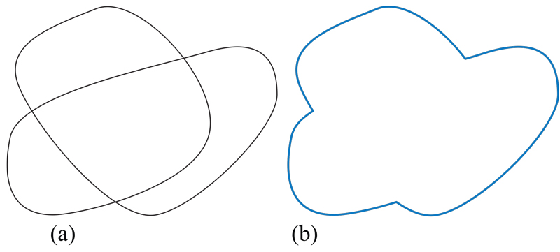
Figure 14.1: (a) Non-simple polygon. (b) Outermost arcs.

∎

Lemma 14.3 ($Z$ Unique).

Let $Z$ be a shortest geodesic polygon enclosing $V$. $Z$ is unique, up to isometry.

Proof.

Assume there is another geodesic polygon $Z^{\prime}$ also enclosing all of $V$ and of the same length: $\ell(Z)=\ell(Z^{\prime})$. Then either one is enclosed in the other, or the two polygons cross at two or more points.

Case 1.

Assume $Z^{\prime}$ is nested inside $Z$.

Case 1a: First assume $Z$ and $Z^{\prime}$ are disjoint. Because all vertices are on or interior to $Z^{\prime}$, $Z$ must be a simple closed geodesic. Let $A$ be the annulus between $Z$ and $Z^{\prime}$; $A$ contains no vertices. Intrinsically, $A$ is a subset of a cylinder with lower circular rim $Z$, and upper boundary $Z^{\prime}$. Thus we can project any point $p\in Z^{\prime}$ orthogonally onto $Z$. See Fig. 14.2(a). Thus $\ell(Z)\leq\ell(Z^{\prime})$, with equality when $Z$ and $Z^{\prime}$ are parallel. In either case, we can “lift” $Z$ parallel to itself until it touches a vertex in $V$. As mentioned earlier, we choose this isometric version of $Z$ as $\min\ell[V]$.

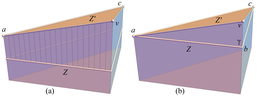
Figure 14.2: $Z^{\prime}=avc$. (a) Edge $av$ projected onto $Z$. (b) ${\gamma}$ with $ab,bc$ forms a planar polygon.

Case 1b: Assume $Z$ and $Z^{\prime}$ share some portion of their boundaries. Again because all vertices are on or inside $Z^{\prime}$, this means that there must be a geodesic arc ${\gamma}$ of $Z$, outside of $Z^{\prime}$, between two shared vertices $v_{1}$ and $v_{2}$. See Fig. 14.2(b). Let $B$ be the region of $P$ bounded by ${\gamma}$ and the edges $E$ of $Z^{\prime}$ between $v_{1}$ and $v_{2}$. Then (a direct induction shows that) $B$ is isometric to a plane polygon, with one straight edge ${\gamma}$, and $E$ a polygonal chain. Therefore $E$ is strictly longer than ${\gamma}$, and so $\ell(Z)<\ell(Z^{\prime})$.

Case 2.

Neither of $Z$ or $Z^{\prime}$ is inside the other. So they must cross at least twice, with always the outer arc a geodesic ${\gamma}$, and the inner sequence of edges possibly containing vertices. Call such a region a lune $L$. Now the argument in Case 1b applies: $L$ is isometric to a planar polygon with straight edge ${\gamma}$, and so the outer arc of $L$ is strictly shorter than the inner arc. Now form $Z^{\prime\prime}$ by following all outer arcs, and otherwise the common portions of the two polygons. $Z^{\prime\prime}$ still encloses all of $V$, but it is strictly shorter than $Z$ and $Z^{\prime}$. This contradiction to the assumption that both $Z$ and $Z^{\prime}$ are shortest establishes the lemma. ∎

This next lemma is a counterpart to the ${\alpha}{\beta}$-converse lemma, Lemma 13.38 in Chapter 13. In the following, a pinned node $v$ of a geoarc polygon $G$ is a flat point which behaves like a vertex, in the sense that $G$ is not allowed to be shorten at $v$ towards its interior.

Lemma 14.4.

Assume that all nodes of a geodesic polygon $G\subset R(Q)$ are either vertices or pinned, and that $V=V(P^{+})\subset R(G)$. Then $G=Z(V)$ if and only if ${\beta}\geq\pi$ at each node of $G$.

Proof.

That ${\beta}\geq\pi$ for $Z(V)$ was established in Lemma 14.1.

In the following we show that $G=Z(V)$, using reasoning similar to that used to prove uniqueness in Lemma 14.3.

In Case 1 of that lemma’s proof, one of $G$ or $Z$ is nested inside the other. Case 1a: Assume the two polygons are disjoint and $Z$ is inside $G$. Then the lemma argument leads to $\ell(G)\leq\ell(Z)$, but because $Z$ is shortest, we must have $\ell(G)=\ell(Z)$; and so $G=Z$. If instead $G$ is inside $Z$, then recall that $Z$ must be a simple closed quasigeodesic. If $Z$ and $G$ are not identical, then the arc of $Z$ between touching points of $G$ is a short-cut of $G$, contradicting the assumption that $G$ has no further short-cuts.

In Case 1b, $G$ and $Z$ share some portion of their boundaries. If $Z$ is inside $G$, the lemma argument shows that $\ell(G)<\ell(Z)$, contradicting the minimality of $Z$. If $G$ is inside $Z$, then consider the region $B$ in the proof of Lemma 14.3, bound by ${\gamma}$ and the edges $E$ of $G$ between $v_{1}$ and $v_{2}$. $B$ is isometric to a plane polygon, and so some vertex along $E$ must be convex. We have thus identified a vertex on $G$ with a right angle ${\beta}<\pi$. So $G$ can be short-cut there, contracting the assumption that no more $G$-short-cuts were possible.

In Case 2, neither is nested in the other, so they must cross. This leads to a polygon shorter than either $G$ or $Z$, a contradiction to the minimality of $Z$. ∎

Example 14.5.

The assumption of pinned nodes in Lemma 14.4 is clearly necessary. Here we show that the second assumption, that $V\subset R(G)$, is also necessary.

Consider an equilateral triangle $abd^{\prime}$ inscribed in the rectangle $abce^{\prime}$, and choose $d\in ce^{\prime}$ between $d^{\prime}$ and $e^{\prime}$, and $e\in ae^{\prime}$ such that $ed\perp bd$. See Figure 14.3. Extend the sides $e^{\prime}a$ and $cb$ sufficiently beyond $a$ and $b$ respectively, and let $L$ be the double of the extended $abcde$. Let $V=\{b,c,d\}$. Note that $e\not\in V$.

On $L$, $Q=aba$ is a simple closed quasigeodesic, and the geodesic polygon $G=bdb$ has each of its angles ${\beta}$ towards $Q$ at least $\pi$. However, $e\notin R(G)$ and $Z(V)=Q$, because $|a-b|=|b-d^{\prime}|<|b-d|$.

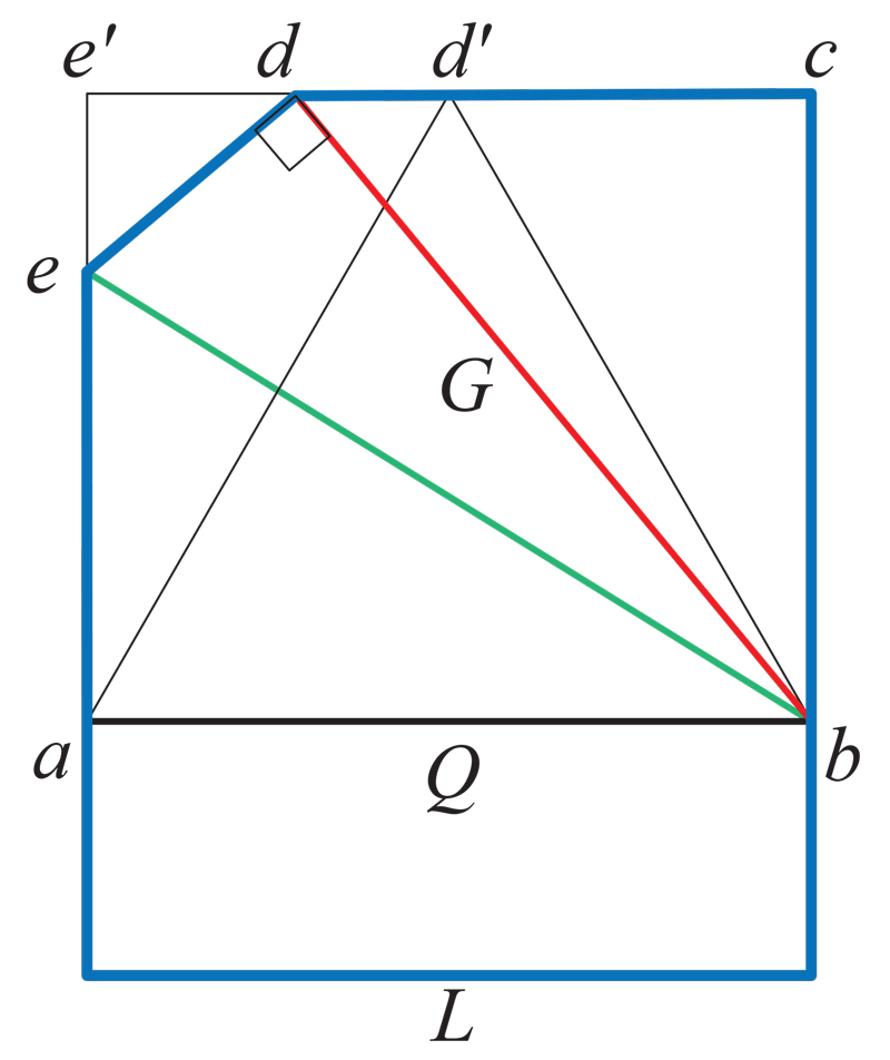
Figure 14.3: Lemma 14.4 is optimal. $V=\{b,c,d\}$, $G=bdb\neq Z=Q$.

We prove here the following result, which will be employed in the next chapter.

Lemma 14.6.

For any point $p\notin V$, $R(Z(V))\,\subseteq\,R(Z(V\cup\{p\}))$.

Proof.

The argument is similar to the one proving the uniqueness of $Z$.

Set $V^{\prime}=V\cup\{p\}$. Clearly, $R(Z(V))=R(Z(V^{\prime}))$ if $p\in R(Z(V))$. So assume that $p$ is strictly exterior to $R(Z(V))$.

Put $I=R(Z(V))\cap R(Z(V^{\prime}))$ and assume there exists $q\in R(Z(V))\setminus R(Z(V^{\prime}))$. If the lemma were to hold, then $I=R(Z(V))$ and $R(Z(V))\setminus R(Z(V^{\prime}))=\varnothing$, so there could be no such $q$. We now prove that the existence of $q$ leads to a contradiction.

Since $V\subset I$ and $q$ is outside $I$, $q$ lies on an geoarc $A\subset Z(V)$ with extremities on $Z(V^{\prime})$. Those extremities determine an arc $A^{\prime}\subset Z(V^{\prime})$ such that $A\cup A^{\prime}$ bounds a flat polygonal domain $L$.

Because of the length minimality of both $Z(V^{\prime})$ and $Z(V)$, $\ell(A^{\prime})=\ell(A)$.

On the other hand, if $A^{\prime}$ is not a geoarc, the flat polygon bounded by $A\cup A^{\prime}$ has the side $A$ necessarily shorter than $A^{\prime}$, a contradiction. And if $A^{\prime}$ is a geoarc, $L$ is a flat digon, contradicting the Gauss-Bonnet Theorem. ∎

14.2 Shortening Algorithm

Our goal in this section is to provide a polynomial-time algorithm to construct $\min\ell[V]$.

14.2.1 Curve-Shortening Flow

Here we digress to highlight the intuition behind curve-shortening. The famous Gage-Hamilton-Grayson (GHG) theorem says that,

If a smooth simple closed curve undergoes the curve-shortening flow, it remains smoothly embedded without self-intersections. It will eventually become convex, and once it does so it will remain convex. … The curve will then converge … to a “round point,” [a vanishingly small circle]. [Wik21]

First assume that all of $V$ is strictly inside $Q$: $Q$ and $V$ are disjoint. At every vertex $u$ of $Q$ strictly convex to its left, replace $u$ with a small arc of a circle, smoothly joined to the incident edges of $Q$. This is now a smooth simple closed convex curve $C$, a smooth approximation of $Q$, to which the GHG theorem applies. Shortening $C$ will either result in a simple closed geodesic, which can no longer be shortened, or it will hit one or more vertices in $V$.

Consider these vertices pinned, partitioning $C$ into sections between pinned vertices. A recent result [ALT12] established that “open curves with fixed endpoints evolving … do not develop singularities, and evolve to geodesics.” Thus the arcs of $C$ between pinned vertices shorten to geodesics. The result is our shortest enclosing geodesic polygon $Z$.

Although there is recent work on discrete curve-shortening, e.g., [AN19] and [EHPN20], it seems it could be difficult to turn this smooth curve-shortening viewpoint into a formal proof or a finite algorithm. So we take a different approach.

14.2.2 Algorithm Overview

We now turn to a discrete, finite algorithm, which we will see is in some sense the reverse of the curve-shortening flow. Imagining $Q$ as roughly equitorial, the flow as described above shortens $Q$ “upward” to $Z$, whereas the algorithm to be described starts with $G$ “above” $Z$ and shortens it “downward” to $Z=\min\ell[V]$.

The algorithm consists of two steps. The first step constructs a geodesic polygon $G$ enclosing $V$. The second step shortens $G$ to $Z$.

14.2.3 Finding an Enclosing Geodesic Polygon

Our goal here is to construct a geodesic polygon $G$ that encloses all vertices in $V$.

It is tempting to build $G$ from the subgraph of the $1$-skeleton of $P$ induced by the vertices in $V$. However, this subgraph is not always connected, as illustrated in Fig. 14.4. As it seems difficult to base an algorithm on this subgraph, we pursue a different approach.

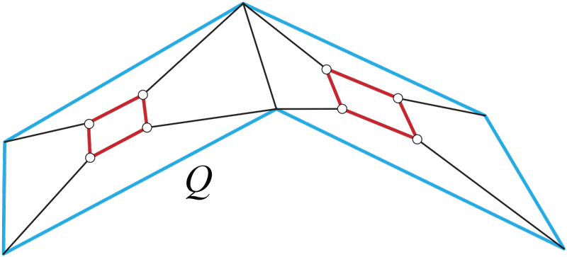
Figure 14.4: $Q$ (blue) encloses $V$, the $8$ marked vertices. The subgraph $V$ induces is the two disconnected red quadrilaterals.

We start by computing all geosegs between pairs of vertices in $V$, and then identify those geoseg subsets (“edgelets”) on the outer boundary of the resulting planar subdivision.

A planar subdivision is a data structure $\mathcal{R}$ that maintains a subset of the plane partitioned into regions. Often called a Planar Straight-Line Graph (PSLG) when its edges are straight-line segments, $\mathcal{R}$ represents an embedding of a planar graph, and maintains the incidence relations between its regions and edges. Such data structures support updates (for us, the addition of new geosegs) in $O(\log n)$ time per intersection.

The algorithm described below has time complexity at worst $O(n^{5}\log n)$, although a careful analysis might lead to $O(n^{4}\log n)$. Our focus is more to show it is polynomial-time, as opposed to optimizing efficiency.

We first describe the three stages of the algorithm at a high-level.

1. Calculate all geosegs between pairs of vertices in $V$. Let ${\Gamma}$ be the collection of these geosegs.

2. Intersect all geosegs in ${\Gamma}$, incrementally building a planar subdivision data structure $\mathcal{R}$ on $P^{+}=R(Q)$. As each $g\in{\Gamma}$ crosses the others already processed, the surface is partitioned into convex regions, call them g-faces bounded by edgelets. Each g-face is flat and isometric to a planar convex polygon; an edgelet is a (generally short) subsegment of a geoseg $g$, between two points where other geosegs cross $g$. G-faces do not necessarily lie in one face of $P$, but they are always empty of strictly interior vertices, or internal edgelets. Fig. 14.5 illustrates a simple such a partition; Fig. 14.7 below is a bit more complicated. As the intersections are calculated, the data structure $\mathcal{R}$ is updated to record ccw orientation of each newly created g-face. The process parallels the incremental algorithm for constructing an arrangement of lines; see Fig. 14.6.

3. Each interior edgelet is shared by exactly two g-faces, recorded in $\mathcal{R}$. A edgelet $e$ shared with just one g-face must be on the boundary of the outer face of the planar subdivision. Connecting all the outer-boundary edgelets yields a geodesic polygon $G$ that encloses all vertices in $V$.

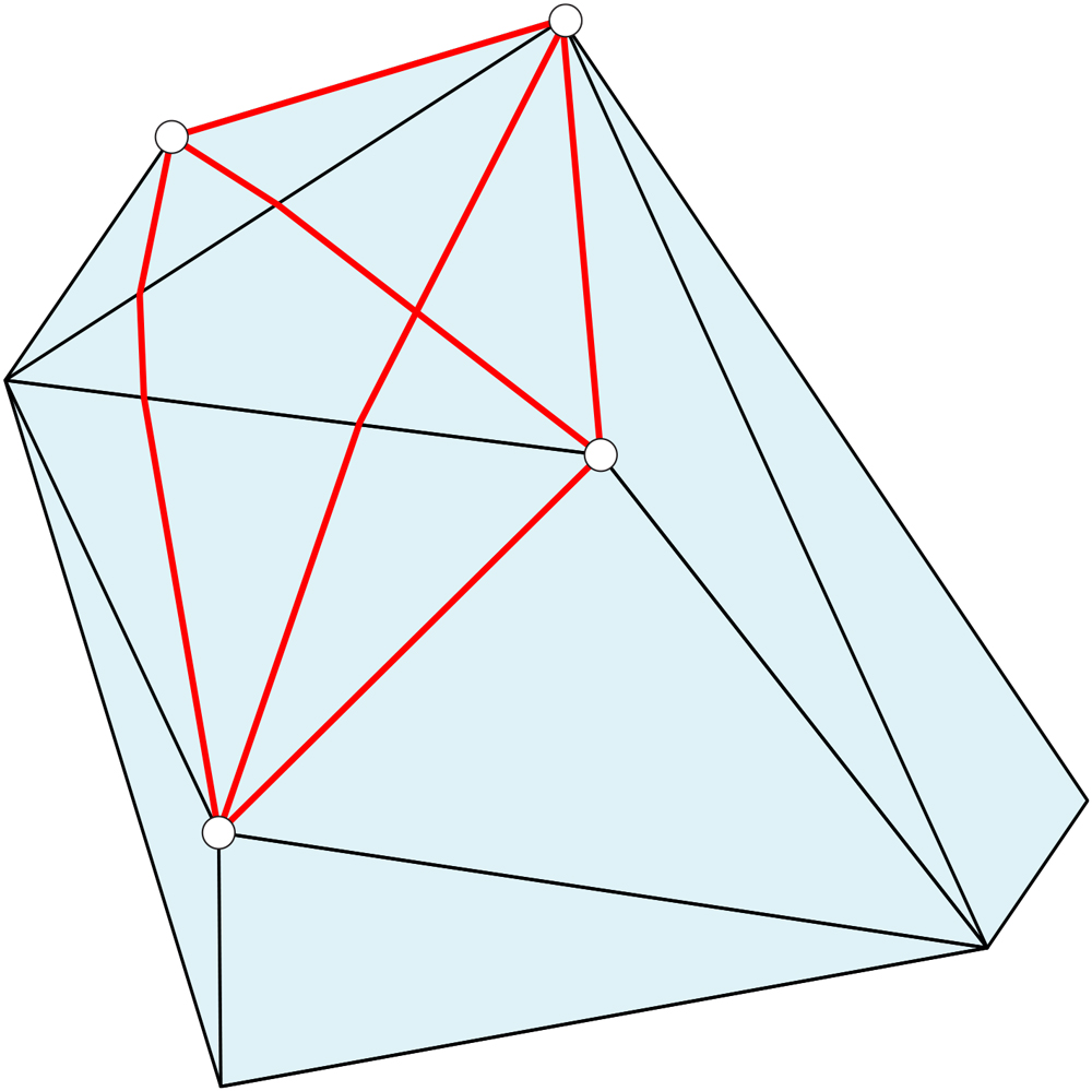
Figure 14.5: $V$ is the four marked vertices. Geosegs (red) form four g-faces.

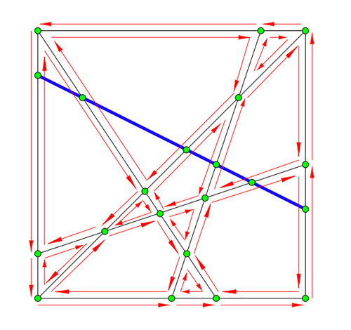
Figure 14.6: Inserting a line into a line-arrangement data structure. (Image from Jan Verschelde Lecture Notes: http://homepages.math.uic.edu/~jan/mcs481/arrangements.pdf)

Next we discuss some computational details for each of the three stages.

1. The total number of geosegs between vertices of $P$ is $O(n^{2})$, each of which can be found in $O(n\log n)$ by the algorithm in [SS08]. Although two vertices may have more than one geoseg connecting them, the number of geosegs from one vertex $v$ and the $n-1$ other vertices is still $O(n)$. This claim can be proved by induction using the cut locus partition (Lemma 2.6 in Chapter 2. For another proof idea, notice that each extra pair of geosegs between two vertices must have a vertex separating them. And there are only $n$ vertices.

2. The total combinatorial size of the data structure $\mathcal{R}$ is $O(n^{4})$, the same size as an arrangement of $\binom{n}{2}$ lines. That each of the $O(n^{4})$ edgelets may cross several edges of $P$ is accounted for in the implicit data structure of [SS08].

3. We note that the sides of $G$ are not necessarily full geosegs between vertices. $G$ in the example shown in Fig. 14.7 includes two edgelets $v_{1}x$ and $v_{3}x$ whose containing geosegs are not wholly on the outer boundary. This example also shows that $G$ is not necessarily convex: it is reflex at $x$.
   The complexity of any face, including the outer face, of an arrangement of segments is just slightly more than linear in the number of segments. Therefore, since $G$ is built from $O(n^{2})$ geosegs, the total number of edgelets on $G$ is $O(n^{2}{\alpha}(n))$, where ${\alpha}$ is the inverse Ackermann function [CEG⁺93].

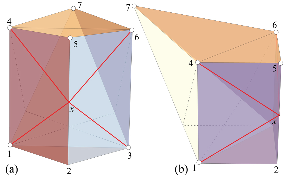
Figure 14.7: $V$ is all the vertices except excluding $v_{2}$. $Q=v_{1}v_{2}v_{3}$. $G=v_{1}xv_{3}v_{1}$. $g_{16}$ and $g_{35}$ (red) on the front are geosegs. The dashed paths around the back are longer and so not geosegs.

A more formal presentation is displayed below as Algorithm 6.

There are two special cases. When $V$ is a single vertex $v$, we allow $G=\{v\}$. And when $|V|=2$, say, $V=\{a,b\}$, $G$ is the ccw loop $aba$.

Input : $n$ vertices $V$ inside or on quasigeodesic $Q$, on $P^{\#}$.

Output : Geodesic polygon $G$ enclosing $V$.

// Calculate all geosegs between pairs of vertices: $O(n^{3}\log n)$.

foreach $\binom{n}{2}$ pairs of vertices in $V$ do

      

      Compute geosegs $v_{i}$ to $v_{j}$, each in $O(n\log n)$ time [SS08].

end foreach

Let ${\Gamma}$ be the set of these $O(n^{2})$ geosegs. // Compute g-faces and edgelets: $O(n^{5}\log n)$.

foreach geoseg $g\in{\Gamma}$ do

       Intersect $g$ with previously built data structure $\mathcal{R}$.

      Create g-face regions, orient each ccw, bounded by edgelets.

      $O(n\log n)$ per geoseg insertion.

end foreach

// Identify outer boundary: $O(n^{4}\log n)$.

foreach edgelet $e$ do

      

      Check in data structure $\mathcal{R}$ if $e$ is shared between two g-faces.

      If not, $e$ is on the boundary of the outer face of the subdivision:

      Then add $e$ to $G$.

end foreach

return $G$.

Algorithm 6 Algorithm to find an enclosing geodesic polygon

We have established this lemma:

Lemma 14.7.

Let $P$ have $n$ vertices, and $V$ a set of vertices in or on quasigeodesic $Q$ (possibly including all vertices of $Q$). Then a geodesic polygon $G$ enclosing all of $V$ can be constructed in $O(n^{5}\log n)$ time.

14.2.4 Algorithm for Curve Shortening

We now describe an algorithm for shortening $G=G_{0}$ to $Z=\min\ell[V]$. We will repeatedly shorten $G_{0}$ to $G_{1},G_{2},\ldots,G_{k}=G$, until $G_{k}=Z$ for some $k\leq n=|V|$. We next describe one shortening step.

Case 1. $|V\cap G_{j}|\geq 3$. Let $v_{i-1},v_{i},v_{i+1}$ be three consecutive nodes of $G_{j}$ (for some $j$), and let ${\alpha}_{i}$ and ${\beta}_{i}$ be the angles at $v_{i}$ left and right of $G_{j}$. If $v_{i}\in Q$, or if ${\beta}_{i}\geq\pi$, we take no action—$G_{j}$ should not or can not be shortened at $v_{i}$. If however $v_{i}\not\in Q$ and ${\beta}_{i}<\pi$, then we can locally shorten $G_{j}$ in a neighborhood of $v_{i}$. But rather than locally shorten, we shorten by replacing the sequence $(v_{i-1},v_{i},v_{i+1})$ by $(v_{i-1},v_{i+1})$. This is a shortening because the triangle inequality holds for geodesic triangles on a convex polyhedron. Let ${\gamma}=v_{i-1}v_{i+1}$.

Before proceeding with the description, we re-examine the example in Fig. 14.8.

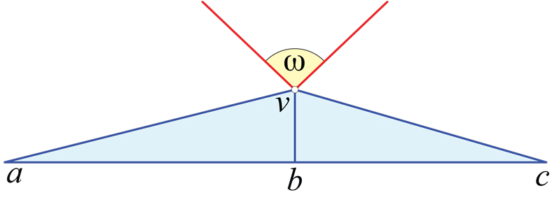
Figure 14.8: Flattening the region between $G$ and $Q$ in Fig. 14.2(b). ${\alpha}\approx 94^{\circ}$, ${\beta}\approx 150^{\circ}$, ${\omega}\approx 116^{\circ}$.

In the example previously shown in Fig. 14.2, we have $G_{0}=(a,v,c)$, and $Q=Z$ as illustrated. Here ${\beta}<\pi$, and flattening the region below $v$ leads to the planar triangle, short-cut by geoarc ${\gamma}=abc$.

Returning to the shortening step, the region of $P^{+}$ between $G_{j}$ and $Q$ is empty of vertices. So the path ${\gamma}$ does not cross any portion of $G_{j}$, nor can it cross $Q$, because the $P^{\#}$ construction would require ${\gamma}$ to cross below and return above $Q$, violating the fact that geodesics do not branch. So the triangle $v_{i-1}v_{i}v_{i+1}$ is between $G_{j}$ and $Q$, and empty of vertices. By the triangle inequality, ${\gamma}$ is shorter than $|v_{i-1}-v_{i}|+|v_{i}-v_{i+1}|$.

Another way to view this construction is to imagine a point $p$ initially at $v_{i}$, sliding down the edge $v_{i-1}v_{i}$ until it reaches $v_{i-1}$. Then the line segment $pv_{i+1}$ never encounters a vertex during this motion, and leads to $pv_{i+1}=v_{i-1}v_{i+1}={\gamma}$.

Applying one of these shortening steps moves a node that was originally on $G$—either a vertex or an intersection of edgelets—to the interior of $G_{j}$. Because the combinatorial size of $G$ is bounded by $O(n^{2}{\alpha}(n))$, there can be no more than that nearly quadratic number of steps.

When no further shortening steps are possible, $G_{k}$ is a geodesic polygon with ${\beta}_{i}\geq\pi$ at every vertex $v_{i}$. By Lemma 14.4 then $G_{k}=Z=\min\ell[V]$.

Before passing to the other cases, we notice that the total curvature ${\omega}$ of $V\subset R(Q)$ is at most $2\pi$.

Case 2. $|V\cap G_{j}|=2$ and $G_{j}$ is a digon with endpoints $v_{1}$ and $v_{2}$. Let ${\beta}_{i}$ be the exterior angles at $v_{i}$, and let $\tau_{i}={\beta}_{i}-\pi$ be the turn angles at $v_{i}$. Gauss-Bonnet requires that ${\omega}+\tau=2\pi$. If both ${\beta}_{i}<\pi$, then $\tau_{1}+\tau_{2}=\tau<0$, and ${\omega}+\tau=2\pi$ cannot be satisfied. If both ${\beta}_{i}\geq\pi$, the algorithm halts. So let ${\beta}_{2}<\pi$.

Because $Q$ is a convex curve, we can merge inside $R(Q)$ all vertices it encloses to obtain one apex $a$ of a cone $\Upsilon$. Clearly, the vertex-free region between $Q$ and $G_{j}$ is isometric to a subset of $\Upsilon$. Unfold $\Upsilon$ by cutting it open along the cone generator $av_{1}$. Then there exists a geodesic loop at $v_{1}$ enclosing $R(G_{j})$ and strictly shorter than $G_{j}$.

A special case is when $|V|=|V\cap G_{j}|=2$ and ${\alpha}_{i}=0$. For example, in Fig. 14.9, with $V=\{c,d\}$, $G=cdc$, and short-cutting at $d$ leads to $Z=cfc$.

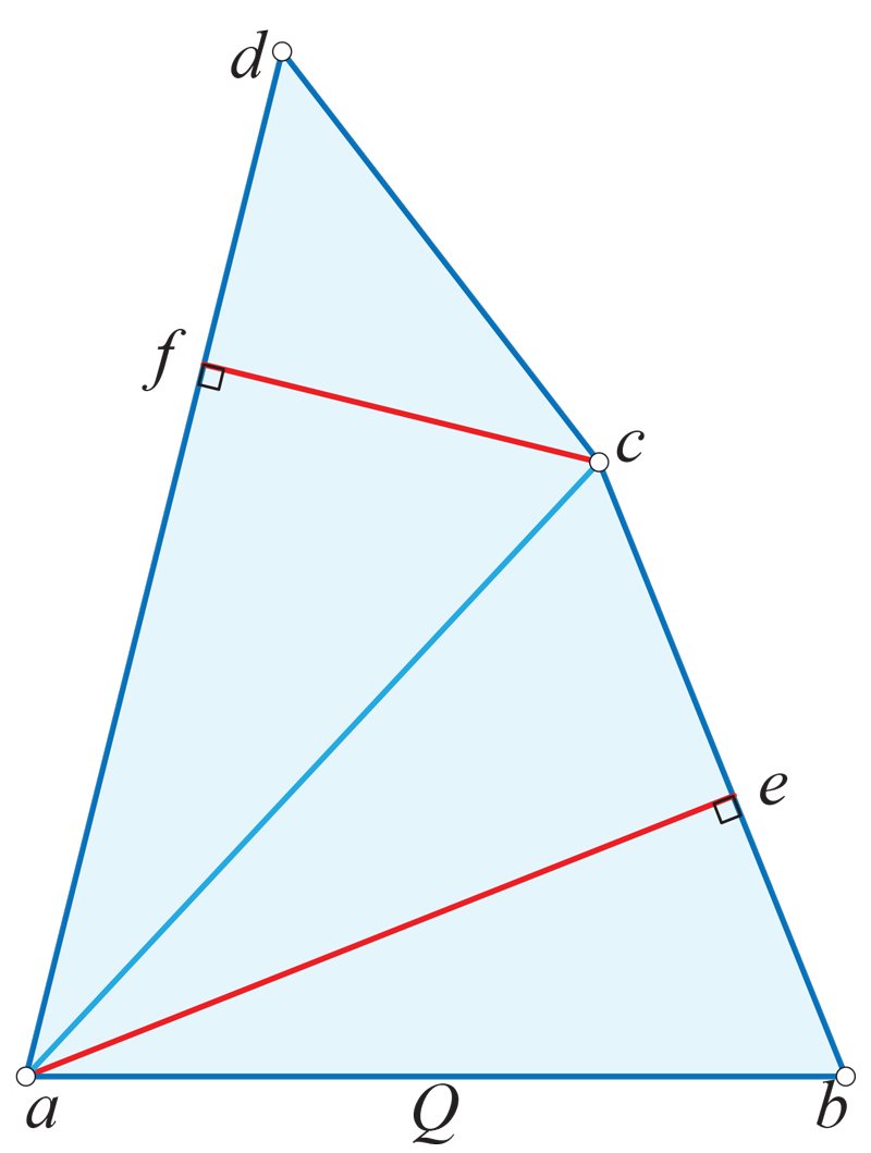
Figure 14.9: Doubly-covered quadrilateral. If $V=\{a,c,d\}$, $G=aca$, $Z=aea$. If $V=\{c,d\}$, $G=cdc$, $Z=cfc$. Vertex $c$ is nonconvex in the doubled $\triangle acd$.

Case 3. $|V\cap G_{j}|=1$. Then $G_{j}$ is a geodesic loop at $v$, where Gauss-Bonnet implies that necessarily ${\beta}\geq\pi$. Therefore the algorithm halts.

This completes the description of the shortening algorithm.

A few remarks on the shortening algorithm:

• The short-cut edge ${\gamma}=v_{i-1}v_{i+1}$ is a geoarc, not a geoseg, because if ${\gamma}$ were a geoseg, it would have been incorporated into the construction of $G=G_{0}$. So every shortening step inserts a geoarc. Later (in Chapter 15), algorithms will vertex-merge along such a geoarc (beyond a geoseg).

• The algorithm relies on the property that the region of $P^{+}$ between $G$ and $Q$ is empty of vertices. All the shortenings insert arcs in this vertex-free region. For that reason, $V$ must include all vertices inside $Q$, i.e., the algorithm may not work if $V$ is a proper subset of the vertices inside $Q$. (However, the construction of $G$ still works, but the shortening may not.) So in this sense, it is not a general “convex hull” algorithm, but rather a construction tailored to our needs.

• The algorithm also works for all vertices inside a convex curve $C$, because doubling $R(C)$ via AGT transforms $C$ into a quasigeodesic.

• Even when $V$ includes all vertices on $Q$, it may be that $G\neq Q$, if $Q$ contains geoarcs. But then the shortening algorithm will result in $Z=Q$.

• Viewing $P^{+}$ as the upper half-surface, one can view $Q$ as the rim of the base of $P^{+}$, $Z$ a closed convex curve “above”/inside $Q$, and $G$ a closed curve “above”/inside $Z$. The shortening algorithm works by, in some sense “area growing” $G$ down to $Z$, even though each growing step is in fact length-shortening. In contrast, the curve-shortening flow described in Section 14.2.1 “raises” $Q$ until it matches $Z$.

We have now established this theorem:

Theorem 14.8 ($Z$-Algorithm).

The minimum-length geodesic polygon enclosing $V$, $Z=Z(V)=\min\ell[V]$, can be constructed in polynomial-time, specifically in time $O(n^{5}\log n)$ where $n=|V|$.

14.3 AG-convexity and $Z$

To parallel the notation $Z=Z(V)=\min\ell[V]$, define $W=W(V)=\partial\,{\rm{rconv}}(V)$.

Lemma 14.9.

The set $R(Z)$ enclosed by $Z=Z(V)$ is a relatively ag-convex set containing $V$, but it is not necessarily equal to ${\rm{rconv}}(V)$.

Proof.

The relative convexity of $R(Z)$ follows directly from the strict ${\alpha}{\beta}$-convexity of $Z$ and Lemma 13.38. The second claim is established by the next example. ∎

Example 14.10.

It could be that $Z(V)\neq W(V)$.

Let $P$ be the octahedron illustrated in Fig. 14.10. The shape is symmetric front-to-back and top-to-bottom. Triangles $acd$ and $ac^{\prime}d^{\prime}$ are congruent $45^{\circ}-45^{\circ}-90^{\circ}$ triangles, and triangles $acc^{\prime}$ and $add^{\prime}$ are congruent equilateral triangles. $Q$ (red) is $aba^{\prime}ea$, and $V=\{a,c,d,a^{\prime}\}$. Let $G=acda^{\prime}$ as illustrated. Then ${\alpha}_{i}<{\beta}_{i}$ at each of the four vertices / gs-nodes. By Lemma 13.38, ${\rm{rconv}}(V)$ is the union of the two triangles $acd$ and $a^{\prime}cd$. However, because ${\beta}$ at both $c$ and $d$ is strictly less than $\pi$, the algorithm would short-cut there, leading to $Z=aba^{\prime}ea=Q$. So $Z(V)\neq W(V)$.

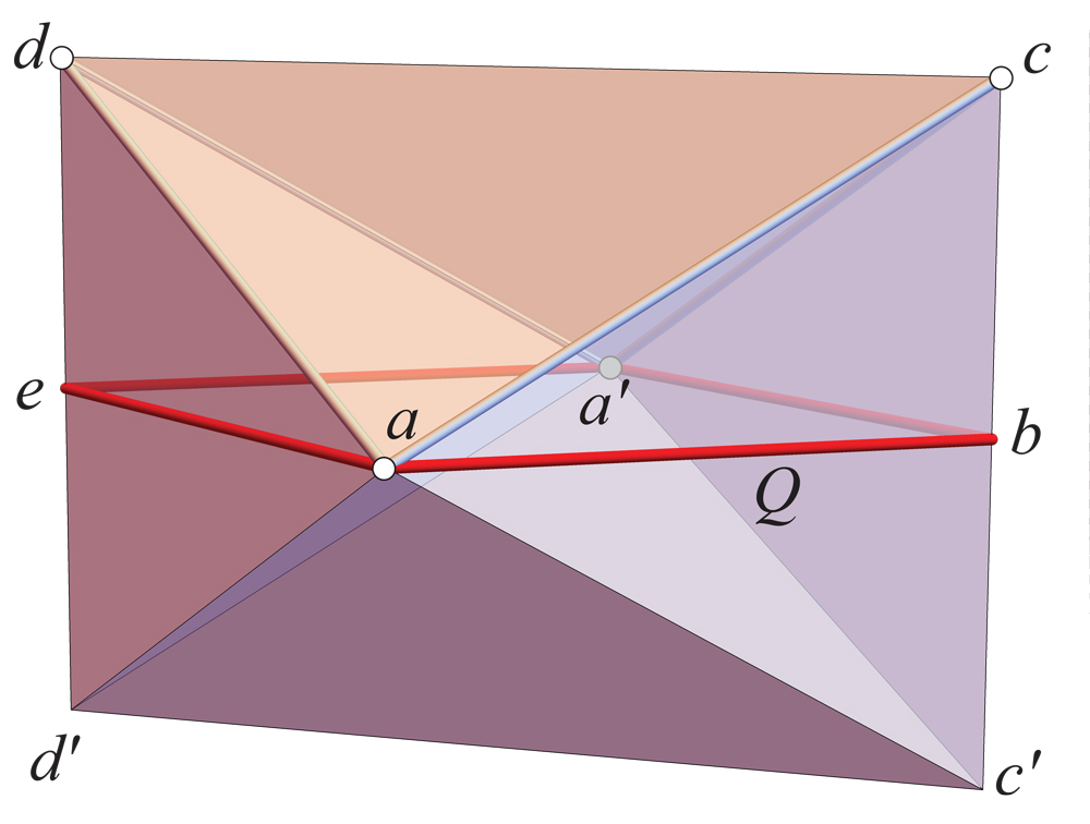
Figure 14.10: $Q=aba^{\prime}ea$, $V=\{a,c,d,a^{\prime}\}$. $Z=aba^{\prime}ea=Q$. $W(V)=aca^{\prime}da$. $Z(V)\neq W(V)$.

It follows, directly from Lemma 14.9 and the definition of ${\rm{rconv}}(V)$, that $R(W)\subseteq R(Z)$, with $Z=Z(V)$ and $W=W(Z)$. So of the two generalizations of the planar convex hull, ${\rm{rconv}}(V)$ is “tighter” than $\min\ell[V]$.

14.4 Algorithm for ${\rm{rconv}}(V)=R(W)$

An algorithm to construct $W=W(V)$ can be obtained by minor modification of the algorithm for $Z=Z(V)$. The first part, calculation of a geodesic polygon $G$ enclosing $V$, is identical. The second part, short-cutting $G$, can be followed with just different criteria of when to short-cut. We will continue to call it a “short-cut” even though it is no longer aimed at length-shortening.

Just as the construction of $Z$ relies on Lemma 14.4, the construction of $W$ relies on the ${\alpha}{\beta}$-converse Lemma 13.38. Assuming the preconditions of these lemmas are satisfied, then the short-cutting decisions of the two algorithm are as follows.

• If $G_{j}$ is such that, for every $v$ on $G_{j}$, ${\beta}\geq\pi$, then $G_{j}=Z$. So we short-cut whenever ${\beta}<\pi$.

• If $G_{j}$ is such that, for every $v$ on $G_{j}$,

  1. if $v$ is a gs-node, then $v$ is strictly ${\alpha}{\beta}$-convex. So we short-cut whenever ${\alpha}\geq{\beta}$. For positive curvature $v$, this implies ${\beta}<\pi$.

  2. if $v$ is a g-node, then $v$ is ${\alpha}{\beta}$-convex. So we short-cut whenever ${\alpha}>{\beta}$. And this implies ${\beta}<\pi$.

  then $G_{j}=W$.

We next explain in some detail how the short-cutting conditions for $W$ imply ${\beta}<\pi$, as claimed in (a) and (b) above. Because ${\alpha}+{\beta}=2\pi$, we have: ${\alpha}\geq{\beta}$ implies that ${\beta}\leq\pi$, and ${\alpha}>{\beta}$ implies that ${\beta}<\pi$. Below we abbreviate “the $Z$-algorithm” and “the $W$-algorithm” with just $Z$ and $W$, for readability.

Positive Curvature $v$.

If $v$ has positive curvature, then ${\alpha}\geq{\beta}$ implies that ${\beta}<\pi$ (because if ${\beta}=\pi$, then ${\alpha}={\beta}=\pi$ and $v$ is flat). So, for positive curvature $v$, whenever $W$ short-cuts, ${\beta}<\pi$ and also $Z$ short-cuts. And for a gs-node, if ${\alpha}<{\beta}$, then $W$ does not short-cut independent of ${\beta}$, but $Z$ will short-cut if ${\beta}<\pi$. And for a g-node, if ${\alpha}\leq{\beta}$, then $W$ does not short-cut independent of ${\beta}$, but $Z$ will short-cut if ${\beta}<\pi$.

Flat $v$.

For flat $v$, if ${\alpha}={\beta}=\pi$, then short-cutting effectively leaves a geodesic through $v$, and so neither algorithm takes action. For flat $v$ and ${\alpha}<{\beta}$, neither algorithm short-cuts: $Z$ because ${\beta}>\pi$; $W$ because strictly ${\alpha}{\beta}$-convex. For flat $v$ and ${\alpha}>{\beta}$, both algorithms short-cut: $Z$ because ${\beta}<\pi$; $W$ because not ${\alpha}{\beta}$-convex.

We have now established this result:

Lemma 14.11.

The $W$-algorithm’s short-cuts are a subset (or equal) to the $Z$-algorithm’s short-cuts.

This accords with our conclusion from Lemma 14.9 that $R(W)\subseteq R(Z)$.

The arguments that the $W$-algorithm’s short-cuts are possible, and that the algorithm halts after at most $n$ steps, are identical to those for the $Z$-algorithm, because every $W$-algorithm short-cut is a $Z$-algorithm short-cut, by Lemma 14.11. So we achieve a result parallel to Theorem 14.8:

Theorem 14.12 ($W$-Algorithm).

The boundary $W(V)$ of ${\rm{rconv}}(V)$ can be constructed in polynomial-time, specifically in time $O(n^{5}\log n)$ where $n=|V|$.

Chapter 15 Spiral Tree on Polyhedron

In the previous chapters we have established the planar model for our spiral tree (based on convex hulls), and the extensions to convex polyhedra of the planar notions of convex hull/minimal length enclosing polygon. In this chapter we continue our program and prove that the spiraling idea works as well for vertex-merging in polyhedral half-surfaces bounded by simple closed quasigeodesics, with respect to either convex hull, or enclosing geodesic polygon.

Although in some sense the 3D algorithm follows the 2D algorithm in Chapter 12 closely, there are several significant differences. One is that, in 2D, no triangles are inserted along each slit, whereas in 3D these insertions change $P$ to a different (larger) polyhedron $P_{i}$ at each step. Another difference is that the 2D slit segments were all geosegs, whereas in 3D some of the slits are geoarcs. These and other differences make the proofs in this chapter somewhat intricate.

15.1 Notation

The notation is a bit complex, so we list the central symbols here for later reference. It may help to refer ahead to Fig. 15.2 to illustrate the definitions below.

• $V=V_{0}=\{v_{1},v_{2},v_{3},\ldots,v_{n}\}$: Vertices on the surface $P$.

• $P_{i}$: Polyhedron after the $i$-th vertex-merge.

• $m_{i}$: merge vertex, the vertex created by merging $m_{i-1}$ with $v_{i+1}$, with $m_{0}=v_{1}$.

• $g_{i}=m_{i-1}v_{i+1}$. The $i$-th slit/merge geoarc.

• $v_{1}$ is also given the label $m_{0}$, so $g_{1}=v_{1}v_{2}=m_{0}v_{2}$.

• $v_{i}$ is called flattened if it has already been merged; the merge will reduce $v_{i}$’s curvature to zero.

• $V_{i}$ is the set of not-flattened vertices on $P_{i}$ remaining after the $i$-th merge along $g_{i}=m_{i-1}v_{i+1}$. $m_{i}\in V_{i}$. $|V_{i}|$ is the number of vertices in $V_{i}$.

• $T^{2}_{i}$ represents the pair of triangles inserted along $g_{i}$ in a vertex-merge, and $T_{i}$ refers to the one of the pair crossed by $g_{i+1}$.

• $H_{i}={\rm{rconv}}(V_{i})$ is the relative ag-convex hull of $V_{i}$, defined in Section 13.7. We view $H_{i}$ as a region of $P_{i}$ and let $\partial H_{i}$ denote its boundary. $H_{0}$ is the convex hull of $V=V_{0}$.

• With some abuse of notation, we identify objects on $P_{i}$ with their image on $P$ and vice-versa.

  For an object $X_{i}$, we put $\tilde{X}_{i}\subset P$ for the image on $P$ of $X_{i}\subset P_{i}$. So, $\tilde{H}_{i}=H_{i}\cap P$, and $\tilde{g}_{i}=g_{i}\cap P$, for all $i$.

• Occasionally, we may also use notation from Chapter 11. For example, as in that chapter, we also identify objects on $P_{i-1}$ with their image on $P_{i}$ and vice-versa.

• $\tilde{{\Lambda}}_{i}=\cup_{i}\,\tilde{g}_{i}$ is the slit graph after the $i$-th merge. $\tilde{{\Lambda}}$ is the full slit graph.

15.2 Icosahedron Example

Before we describe and prove the spiral algorithm in Section 15.3, we illustrate its application to an icosahedron $P$. This repeats our discussion in Section 11.4 but following a spiral sequence of vm-reductions. In Chapter 11 the endpoint of the reductions was the doubly-covered triangle shown in Fig. 11.7. Here the endpoint of the reductions will be a half-cylinder, described in the next chapter (Fig. 16.9).

We label the $12$ vertices of $P$ as shown in Fig. 15.1. $Q$ is a simple closed geodesic around the “equator” of the icosahedron, and $V$ the six vertices above $Q$, $v_{1},v_{2},v_{3},v_{4},v_{5},v_{6}$. The vertices are merged in that order, as indicated in Fig. 15.1. (This differs from the order in Section 11.4, which merged $v_{1},v_{2},v_{3},v_{4},v_{6}$, leaving $v_{5}$ unmerged.)

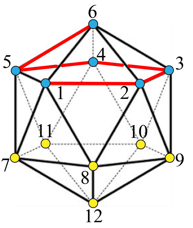
Figure 15.1: Labels $i$ for vertices $v_{i}$. Sequential merge path in red. Cf. Fig. 11.5.

Each of the five merges $i$ is accomplished by inserting two copies of a triangle $T_{i}$, whose apex is the merge vertex $m_{i}$. By convention $m_{0}=v_{1}$. For $i=1,\ldots,5$,

$$m_{i-1}\;+\;v_{i+1}\;\to\;m_{i}\;,\;T_{i}\;\textrm{along}\;g_{i}\;.$$

Here $m_{5}$ is special for the icosahedron in that $T_{5}$ is actually an infinite parallelogram sending $m_{5}$ off to $z=+\infty$, because the sum of the curvatures of $v_{1},\ldots,v_{6}$ is exactly $2\pi$.

Now we describe the steps of the algorithm, referring to Fig. 15.2 throughout.

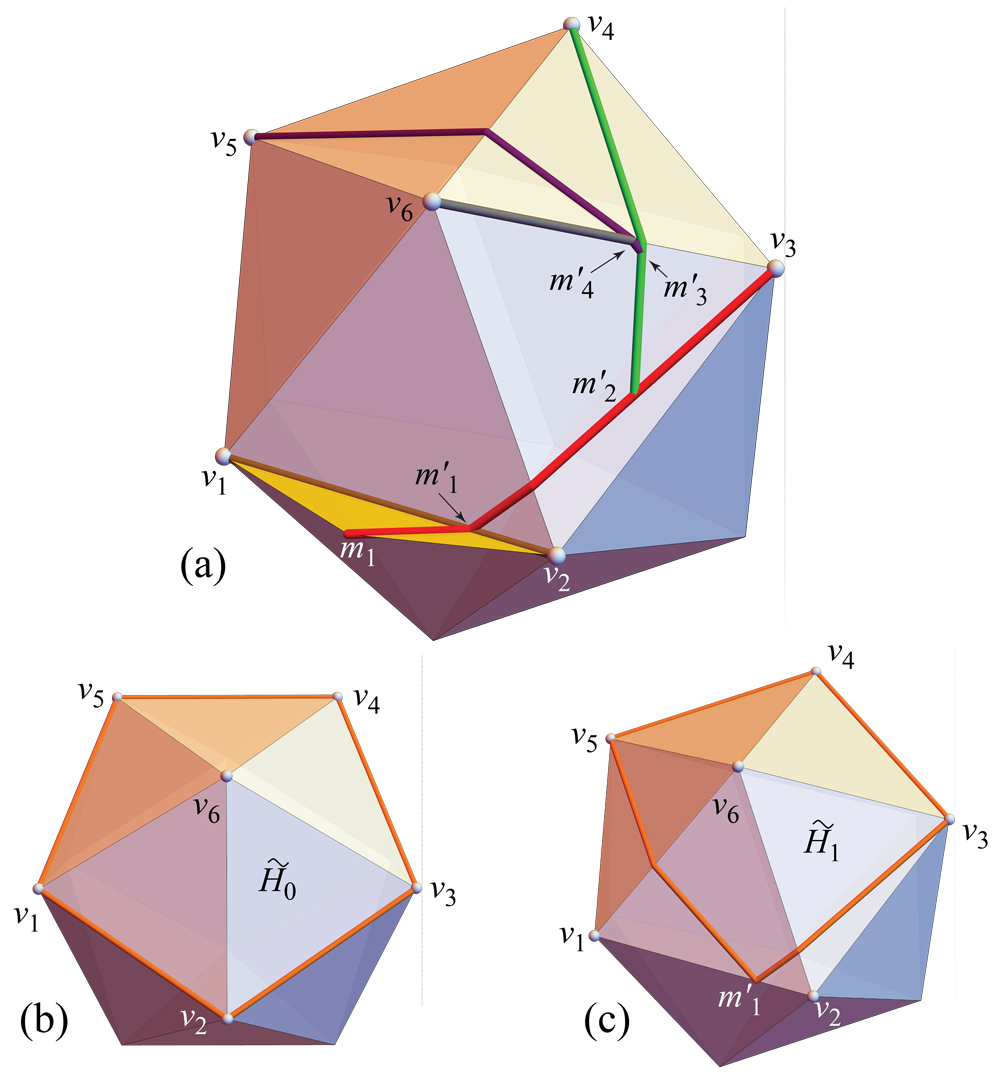
Figure 15.2: (a) Five geodesic slits ${\gamma}_{i}$ on $P$, each entering $P$ from $T_{i}$ at $m^{\prime}_{i}$. (b,c) $\tilde{H}_{0}$ and $\tilde{H}_{1}$. Cf. Fig. 11.6.

With $V=V_{0}$ on $P=P_{0}$, the initial convex hull containing $V_{0}$ is ${\rm{rconv}}(V_{0})=H_{0}=\tilde{H}_{0}$, with $\partial H_{0}=v_{1}v_{2}v_{3}v_{4}v_{5}$. See Fig. 15.2(b).

The first step, $i{=}1$, merges two consecutive vertices of $\partial H_{0}$, say $v_{1}$ and $v_{2}$ (as illustrated). So the slit segment is $g_{1}=v_{1}v_{2}=m_{0}v_{2}$, where $v_{1}=m_{0}$. Doubled triangles $T^{2}_{1}$ are inserted along $g_{1}$, which flatten $v_{1}$ and $v_{2}$, and introduces a new vertex $m_{1}$ at the apex of the triangles. The result is a new polyhedron $P_{1}$. We cannot easily illustrate $P_{1}$ (because of the nonconstructive nature of AGT), but it can be imagined from the (yellow) triangle $T_{1}$ shown attached to $v_{1}v_{2}$ in Fig. 15.2(a).

On $P_{1}$, $V_{1}=\{m_{1},v_{3},v_{4},v_{5},v_{6}\}$. $H_{1}={\rm{rconv}}(V_{1})$, with $\partial H_{1}=m_{1}v_{3}v_{4}v_{5}$, with $m_{1}v_{3}$ a geodesic from the apex $m_{1}$ of $T_{1}$, to $m^{\prime}_{1}$ where it enters $P$, and then on $P$ to $v_{3}$. $\tilde{H}_{1}$ has boundary $\partial\tilde{H}_{1}=m^{\prime}_{1}v_{3}v_{4}v_{6}$, as shown in Fig. 15.2(c). Notice that $\tilde{H}_{1}\subset\tilde{H}_{0}$ on $P$, but $H_{1}\not\subset H_{0}$ on $P_{1}$: $m_{1}\not\in H_{0}$.

$P_{2}$ is obtained by inserting $T^{2}_{2}$ triangles along the slit $g_{2}$ connecting $m_{1}$ to $v_{3}$, red in Fig. 15.2(a). These triangles flatten $m_{1}$ and $v_{3}$, leaving $V_{2}=\{m_{2},v_{4},v_{5},v_{6}\}$, and $H_{2}={\rm{rconv}}(V_{2})$, with $\partial H_{2}=m_{2}v_{4}v_{5}$ and $\partial\tilde{H}_{2}=m^{\prime}_{2}v_{4}v_{5}$.

The process continues, with the final set of slits as depicted in Fig. 15.2(a). Note that, on $P$, each slit $\tilde{g}_{i}$ starts from a point $m^{\prime}_{i-1}$ on $\tilde{g}_{i-1}$ and ends at $v_{i+1}$.

15.3 Spiraling Algorithm for ${\rm{rconv}}$

First Step.

As described above in the icosahedron example, $H_{0}={\rm{rconv}}(V)$ is computed via the algorithm described in Section 14.4. Two vertex endpoints of an edge of $\partial H_{0}$, $v_{1}=m_{0}$ and $v_{2}$, are merged along $g_{1}=m_{0}v_{2}$. Triangles $T^{2}_{1}$ are inserted along $g_{1}$, flattening $v_{1}$ and $v_{2}$ and introducing a merge vertex $m_{1}$. Now $V_{1}=(V\setminus\{v_{1},v_{2}\})\cup\{m_{1}\}$ and $H_{1}={\rm{rconv}}(V_{1})$.

General Step.

We now describe the general step, referring to Fig. 15.3. Suppose step $i-1$ has been completed. $H_{i-1}={\rm{rconv}}(V_{i-1})$ is on $P_{i-1}$, with $V_{i-1}=\{m_{i-1},v_{i+1},\ldots\}$. The merge vertex $m_{i-1}$ is a vertex of $\partial H_{i-1}$, and $v_{i+1}$ is the next vertex of that hull boundary, counterclockwise.

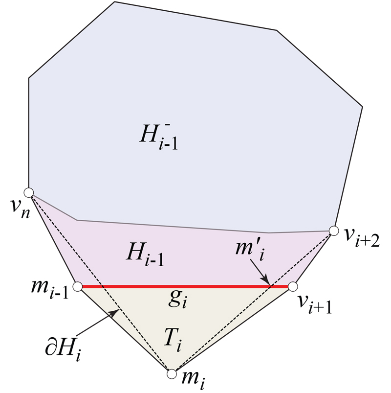
Figure 15.3: $H_{i-1}$ and $H_{i}$ on $P_{i}$.

For the $i$-th step, we consider two cases:

Case 1: $m_{i-1}\neq v_{i+1}$. Then $g_{i}=m_{i-1}v_{i+1}$ is an edge of $\partial H_{i-1}$. Triangles $T^{2}_{i}$ are inserted along $g_{i}$, flattening $m_{i-1}$ and $v_{i+1}$, and forming $P_{i}$. $V_{i}$ loses these two vertices and gains the new merge vertex $m_{i}$. $H_{i}={\rm{rconv}}(V_{i})$.

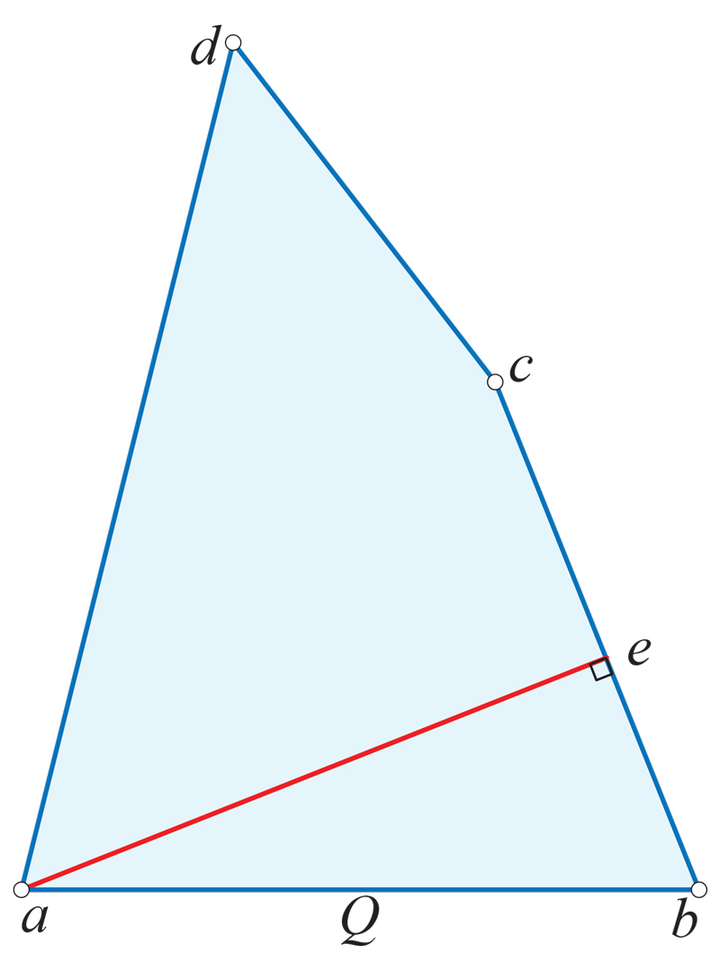
Figure 15.4: Double-sided quadrilateral, $Q=(a,b,a)$. The path $(a,e,a)$ is a geodesic loop. For $V=\{a,c,d\}$, $\partial\,{\rm{rconv}}(V)=(a,e,a)$.

Case 2: $m_{i-1}=v_{i+1}$, hence $\partial H_{i-1}$ is a geodesic loop. We have seen that this case can occur. For example, in Fig. 15.4, $(a,e,a)$ is a geodesic loop. (See Example 13.31 for the proof.) In such a case, $\partial H_{i-1}$ consists only of the vertex $m_{i-1}$, and a geodesic loop at $m_{i-1}$. Clearly we cannot execute vertex-merging along such a loop, so we need another strategy for this exceptional case.

Let $V^{\prime}_{i-1}=V_{i-1}\setminus\{m_{i-1}\}$. Construct $H^{\prime}_{i-1}={\rm{rconv}}V^{\prime}_{i-1}$, and let $p$ be the point on $\partial H^{\prime}_{i-1}$ closest to $m_{i-1}$, say $p\in{\gamma}$, where ${\gamma}$ is a geoarc of $\partial H^{\prime}_{i-1}$. Notice that either $p$ is a vertex of $V^{\prime}_{i-1}$, or there is a unique geoseg from $m_{i-1}$ to $p$, which in particular is orthogonal to ${\gamma}$ at $p$.

If $p$ is a vertex of $V^{\prime}_{i-1}$, take $g_{i}=m_{i-1}p$ and notice that $g_{i}$ intersects neither $\partial H_{i-1}$ nor $\partial H^{\prime}_{i-1}$, other than at $m_{i-1}$ and at $p$, respectively, by construction.

Assume now that $p$ is a flat point of $H^{\prime}_{i-1}$, hence interior to ${\gamma}$. Then take $v_{i+1}$ to be either endpoint-vertex of ${\gamma}$ (or the only vertex on ${\gamma}$ if ${\gamma}$ is a geodesic loop). Next we show there exists a geoarc $g_{i}=m_{i-1}v_{i+1}$ intersecting neither $\partial H_{i-1}$, nor $\partial H^{\prime}_{i-1}$, other than at $m_{i-1}$ and at $v_{i+1}$, respectively.

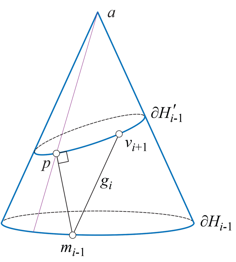
Figure 15.5: On the cone $\Upsilon$, $g_{i}=m_{i-1}v_{i+1}$ crosses neither $\partial H_{i-1}$ nor $\partial H^{\prime}_{i-1}$.

Notice first that $V^{\prime}_{i-1}$ is strictly interior to $H_{i-1}$ (because $\partial H_{i-1}$ only contains the one vertex $m_{i-1}$), hence so is $H^{\prime}_{i-1}={\rm{rconv}}(V^{\prime}_{i-1})$ (by Lemma 13.15, the interior of a convex set is convex). Therefore, $\partial H_{i-1}\cap\partial H^{\prime}_{i-1}=\varnothing$.

Because both $\partial H_{i-1}$ and $\partial H^{\prime}_{i-1}$ are convex curves, we can merge all vertices of $V^{\prime}_{i-1}$ to obtain one apex $a$ of a cone $\Upsilon$. It follows that both $\partial H_{i-1}$ and $\partial H^{\prime}_{i-1}$ “live on $\Upsilon$,” in the sense that the closed region $A$ of $P_{i-i}$ they bound is isometric to a subset of $\Upsilon$ containing $a$. (For details see [OV14].) Refer to Fig. 15.5.

Unfold $A$ by cutting it open along the cone generator through $ap$. Also denote by $A$ the result. Then (the images of) $\partial H_{i-1}$ and $\partial H^{\prime}_{i-1}$ are convex planar curves in $A$, and $m_{i-1}p\perp{\gamma}\subset\partial H^{\prime}_{i-1}$. Then we see that $g_{i}=m_{i-1}v_{i+1}$ again intersects neither $\partial H_{i-1}$ nor $\partial H^{\prime}_{i-1}$ except at its endpoints.

Lemma 15.1.

The new merge vertex $m_{i}$ created at step $i$ is on $\partial H_{i}$ (as opposed to strictly interior to $\partial H_{i}$).

Proof.

The algorithm constructs $H_{i}$ by removing the two flattened vertices $m_{i-1}$ and $v_{i+1}$ and adding the new merge vertex $m_{i}$. Formally,

$$H_{i}={\rm{rconv}}\left(\,(V_{i-1}\setminus\{m_{i-1},v_{i+1}\})\cup\{m_{i}\}\right)\;.$$

Let $H^{-}_{i-1}={\rm{rconv}}(V_{i-1}\setminus\{m_{i-1},v_{i+1}\})$, i.e., the relative convex hull of $V_{i-1}$ with the flattened vertices removed, but the new merge vertex $m_{i}$ not yet added. See Fig. 15.3. The geoarc $g_{i}=m_{i-1}v_{i+1}$ is strictly exterior to $H^{-}_{i-1}$, because it is included in $\partial H_{i-1}$. Now attach the doubled $T^{2}_{i}$ triangle to $g_{i}$, with triangle apex $m_{i}$. It is clear that $m_{i}$ is also strictly exterior to $H^{-}_{i-1}$: some points on a geoseg from $m_{i}$ to a point in $H^{-}_{i-1}$ must be exterior to $H^{-}_{i-1}$. So $m_{i}\not\in H^{-}_{i-1}$. Therefore, with $H_{i}={\rm{rconv}}(H^{-}_{i-1}\cup m_{i})$, it must be that $m_{i}$ is a vertex of $\partial H_{i}$.

For the exceptional geodesic-loop case of the algorithm, the conclusion follows by construction. ∎

Notice that $H_{i-1}$ is not necessarily closed, which in some circumstances leads to $\partial H_{i-1}$ being not strictly ${\alpha}{\beta}$-convex, but it remains nevertheless ${\alpha}{\beta}$-convex. See Lemma 13.6 and Example 13.7 concerning ${\alpha}{\beta}$-convexity.

Lemma 15.2 (Visibility).

Let ${\gamma}$ be the geoarc connecting the new merge vertex $m_{i}$ created at step $i$ to the next vertex $v_{i+2}$ to be merged. Then ${\gamma}$ crosses the geoarc $g_{i}$ at a point $\{m^{\prime}_{i}\}=g_{i}\cap{\gamma}$. In a sense, $v_{i+2}$ is “visible” to $m_{i}$ through $g_{i}$.

Proof.

We use the ${\alpha}{\beta}$-convexity property of $\partial H_{i-1}$: the angles ${\alpha}_{i+1},{\beta}_{i+1}$ at the $v_{i+1}$ endpoint of the geoarc $g_{i}=m_{i-1}v_{i+1}$ satisfy ${\alpha}_{i+1}\leq{\beta}_{i+1}$.

We aim to show that, after insertion of the double triangle along $g_{i}$, the new angle at $v_{i+1}$, $\angle m_{i}v_{i+1}v_{i+2}$, is convex, which proves the claim of the lemma.

So we aim to prove that ${\alpha}_{i+1}+\frac{1}{2}{\omega}_{i+1}\leq\pi$; the factor $\frac{1}{2}$ appears because that is the angle of $T_{i}$’s corner at $v_{i+1}$. To simplify the derivation, we suppress the index $i+1$; so the goal is ${\alpha}+\frac{1}{2}{\omega}\leq\pi$. Because the triangle insertion flattens $v_{i+1}$, we know that ${\omega}=2\pi-({\alpha}+{\beta})$. So we get equivalent inequalities:

$${\alpha}+\tfrac{1}{2}{\omega} \leq\pi$$

$${\alpha}+\pi-\tfrac{1}{2}{\alpha}-\tfrac{1}{2}{\beta} \leq\pi$$

$$\tfrac{1}{2}{\alpha} \leq\tfrac{1}{2}{\beta}$$

which holds at $v_{i+1}$ by ${\alpha}{\beta}$-convexity.

The same argument applies to the other endpoint $m_{i-1}$ of $g_{i}$. ∎

This lemma verifies that the drawing in Fig. 15.3 is a correct depiction. If this lemma did not hold, then ${\gamma}=m_{i}v_{i+2}$ would not necessarily cross $g_{i}$.

15.4 Proof: Slit Graph is a Tree

The next lemma is the counterpart to the nesting property of the 2D spiral algorithm, previously illustrated in Fig. 12.4.

Lemma 15.3 (Nesting).

$\tilde{H}_{i}\subset\tilde{H}_{i-1}$.

It may be useful to keep in mind the situation on $P_{i}$ in Fig. 15.3, and the $\tilde{H}_{i}$ examples on $P$ in Fig. 15.2(bc), which shows $\tilde{H}_{1}\subset\tilde{H}_{0}$. With some abuse of notation in the proof, we will identify objects on $P_{i-1}$ with their image on $P_{i}$ and vice-versa.

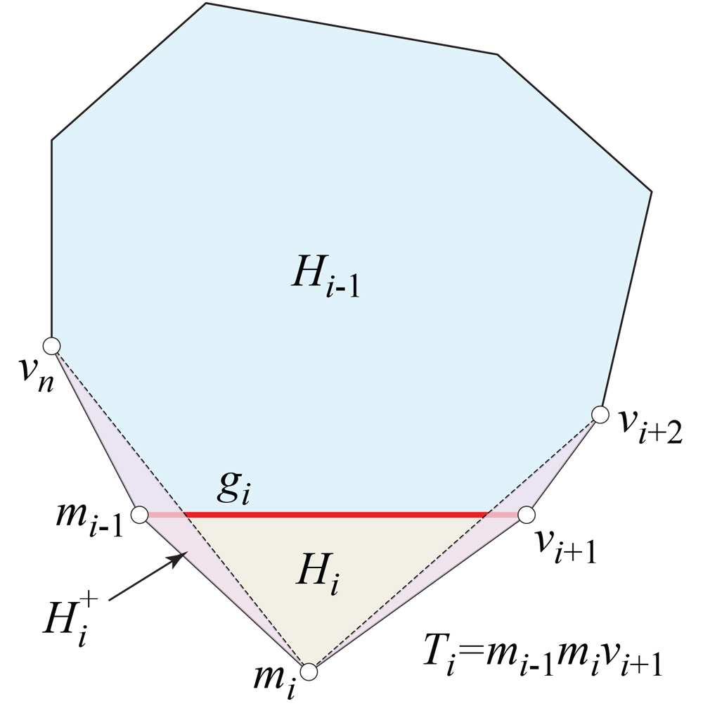
Figure 15.6: $H_{i}\subset H^{+}_{i}$.

Proof.

The proof is in two parts. We show first that $\tilde{H}_{i}\subset\tilde{H}_{i-1}$. Set $V^{-}_{i-1}=V_{i-1}\setminus\{m_{i-1},v_{i+1}\}$, i.e., $V_{i-1}$ without the two vertices that will form the next vertex-merge insertion. To keep track of the notation, we refer to Fig. 15.6 (a variation of Fig. 15.3) and this display, where we use “$-$” to indicate “missing” vertices among the three $m_{i-1},m_{i},v_{i+1}$:

$$\;\;V^{-}_{i-1}=\{v_{i+2},\ldots,v_{n}\}$$

$$H_{i-1}={\rm{rconv}}(V_{i-1})\;, \;\;V_{i-1}=\{m_{i-1},-,v_{i+1}\}\cup V^{-}_{i-1}$$

$$H_{i}={\rm{rconv}}(V_{i})\;, \;\;V_{i}=\{-,m_{i},-,\}\cup V^{-}_{i-1}$$

$$H^{+}_{i}={\rm{rconv}}(V^{+}_{i})\;, \;\;V_{i}=\{m_{i-1},m_{i},v_{i+1}\}\cup V^{-}_{i-1}$$

Set $H^{+}_{i}$ as above. Then as Fig. 15.6 shows, $H_{i}\subset H^{+}_{i}$ and thus $\tilde{H}_{i}\subset\tilde{H}^{+}_{i}$.

Denote by $T_{i}=\triangle m_{i-1}m_{i}v_{i+1}$ one of the two inserted triangles along $g_{i}$, the one sharing $g_{i}$ in common with $H_{i-1}$.

For the second part of the proof, we next show that, on $P_{i}$, $H^{+}_{i}=H_{i-1}\cup T_{i}$. First, notice that $H_{i-1}\cup T_{i}\subset H^{+}_{i}$ (by Lemma 13.24 on the hull of a set partition), so ${\rm{rconv}}(H_{i-1}\cup T_{i})\subset H^{+}_{i}$. Second, the ${\alpha}{\beta}$-convexity of $\partial H_{i-1}$ at $m_{i-1}$ and $v_{i+1}$ on $P_{i-1}$ shows that, on $P_{i}$, the two sides of $T_{i}$ incident to $m_{i}$ either extend two boundary arcs of $H_{i-1}$ (if the ${\alpha}{\beta}$-convexity is not strict), or they make with the respective boundary arcs angles $<\pi$ towards $H_{i-1}\cup T_{i}$ (if the ${\alpha}{\beta}$-convexity is strict); see Lemma 15.2 (Visiblity). Therefore, $H_{i-1}\cup T_{i}$ is a convex set (by Lemma 13.38) containing $V^{-}_{i-1}\cup\{m_{i-1},m_{i},v_{i+1}\}$, hence $H_{i-1}\cup T_{i}\supset{\rm{rconv}}(V^{-}_{i-1}\cup\{m_{i-1},m_{i},v_{i+1}\})=H^{+}_{i}$.

Finally, since $H^{+}_{i}=H_{i-1}\cup T_{i}$ and the image on $P$ of $T_{i}$ is a subarc of $\tilde{g}_{i}$, we have $\tilde{H}^{+}_{i}=\tilde{H}_{i-1}$.

In conclusion, $\tilde{H}_{i}\subset\tilde{H}^{+}_{i}=\tilde{H}_{i-1}$. ∎

Notice that, unlike the planar case where $g_{i}$ only intersects $H_{i}$ in one point, $g_{i}\cap H_{i}=\{m_{i}\}$ (Fig. 12.2(b)), on polyhedra $g_{i}$ intersects $H_{i}$ on a sub-segment (Fig. 15.3).

Recall that, in our notation, $g_{i-1}$ is a curve (a geoarc) on $P_{i-2}$ and $g_{i}$ is a curve on $P_{i-1}$.

Lemma 15.4 ($g_{i}\cap g_{i-1}$).

On $P_{i-1}$, $g_{i}$ intersects the two images (“banks”) of $g_{i-1}$ at precisely one point. Consequently, $\tilde{g}_{i}$ has an endpoint on $\tilde{g}_{i-1}$ and no other common point.

Proof.

On $P_{i-1}$, $g_{i}$ joins the point $m_{i-1}$ to a vertex $v_{i+1}$. But $m_{i-1}$ is inside the inserted region (a pair of triangles) $T_{i-1}$, while $v_{i+1}$ is outside $T_{i-1}$. Remember that the boundary of $T_{i-1}$ consists of two copies of $g_{i-1}$, say $g^{\prime}_{i-1}$ and $g^{\prime\prime}_{i-1}$. So $g_{i}$ intersects those two copies, $g^{\prime}_{i-1}\cup g^{\prime\prime}_{i-1}$, at least once.

Assume, for the sake of contradiction, that there are two distinct points

$$x^{\prime},x^{\prime\prime}\in g_{i}\cap(g^{\prime}_{i-1}\cup g^{\prime\prime}_{i-1})\;.$$

Assume first that $\{x^{\prime}\}=g_{i}\cap g^{\prime}_{i-1}$ and $\{x^{\prime\prime}\}=g_{i}\cap g^{\prime\prime}_{i-1}$. It follows that $g_{i}$ exits $T_{i-1}$ and enters it again, and so to reach $v_{i+1}$ it has to exit $T_{i-1}$ again, crossing $g^{\prime}_{i-1}\cup g^{\prime\prime}_{i-1}$ once more. Therefore, we may assume next that both $x^{\prime}$ and $x^{\prime\prime}$ arise from $g_{i}$ intersecting one $g_{i-1}$ image, say $g^{\prime}_{i-1}$. Hence $g_{i}$ and $g^{\prime}_{i-1}$ determine a geodesic digon, which necessarily contains a vertex $v\in V$ (by the Gauss-Bonnet Theorem). Since there is no vertex both outside $H_{i-1}$ and inside $H_{i-2}$, and there is no vertex both outside $H_{i-2}$ and inside $H_{i-1}$ other than $m_{i-1}$, a contradiction is obtained.

Therefore, $g_{i}$ intersects the two images of $g_{i-1}$ at precisely one point, and thus we get that $|\tilde{g}_{i-1}\cap\tilde{g}_{i}|=1$. ∎

Lemma 15.5.

The set of vertices reduces by one each iteration: $|V_{i}|=|V_{i-1}|-1$, for $i>1$.

Proof.

Clearly $|V_{i}|=|V_{i-1}|-1$, because $V_{i}=V_{i-1}\setminus\{m_{i-1},v_{i+1}\}\cup\{m_{i}\}$. ∎

Lemma 15.6.

$\tilde{{\Lambda}}_{i}$ is a tree.

Proof.

By Lemma 15.4 above, $\tilde{g}_{i}$ has an endpoint on $\tilde{g}_{i-1}$, and otherwise does not intersect $\tilde{g}_{i-1}$. It remains to prove that the interaction of $\tilde{g}_{i}$ with the earlier segments in $\tilde{{\Lambda}}_{i}$ maintains the tree property. In fact, we show that $\tilde{g}_{i}\cap\tilde{g}_{j}=\varnothing$ for $j<i-1$.

By our sequential-merge choice, $g_{i}$ is an edge $e=m_{i-1}v_{i+1}$ of $\partial H_{i-1}$, and so $\tilde{g}_{i}$ is an edge $\tilde{e}$ of $\partial\tilde{H}_{i-1}$. For example, in Fig. 15.2(bc), $\tilde{g}_{1}=v_{1}v_{2}$ is an edge of $\tilde{H}_{0}$, and $\tilde{g}_{2}=m^{\prime}_{1}v_{3}$ is an edge of $\tilde{H}_{1}$.

From Lemma 15.3 (Nesting) we know that $\tilde{H}_{j}\supset\tilde{H}_{i-1}$ for $j<i-1$.

Therefore, $\tilde{g}_{j}\cap\tilde{H}_{i-1}$ is either the empty set, or an edge of $\tilde{H}_{i-1}$, so it cannot intersect other edges of $\tilde{H}_{i-1}$ excepting those adjacent to it (by Theorem 13.40, which established the simplicity of ${\rm{rconv}}$ boundaries).

Since the edge $\tilde{g}_{i-1}\cap\tilde{H}_{i-1}$ is between $\tilde{g}_{j}\cap\tilde{H}_{i-1}$ (not empty by Lemma 11.1) and $\tilde{g}_{i}$ (“between” with respect to the circular order of sides in $\partial\tilde{H}_{i-1}$), $\tilde{g}_{j}$ cannot intersect $\tilde{g}_{i}$ for $j<i-1$.

For example, returning to Fig. 15.2, when $i=3$ and $j=1$, we have $\tilde{H}_{i-1}=\tilde{H}_{2}$, $\tilde{g}_{i}=\tilde{g}_{3}=m^{\prime}_{2}v_{4}$, $\tilde{g}_{j}=\tilde{g}_{1}=v_{1}v_{2}$, and indeed $\tilde{g}_{1}$ does not intersect $\tilde{g}_{3}$.

Therefore, we have shown that $\tilde{g}_{i}$ just intersects $\tilde{{\Lambda}}_{i-1}$ at the one point, and so maintains the tree structure for $\tilde{{\Lambda}}_{i}$. ∎

Putting together the above lemmas yields the following theorem, one of our primary goals.

Theorem 15.7.

Let $Q$ be a simple closed quasigeodesic on the convex polyhedron $P$, and $V$ the set of vertices of $P$ enclosed by $Q$, to either side of $Q$. Then the sequential vertex-merging algorithm detailed in Section 12.3 results in a slit graph $\tilde{{\Lambda}}$ that is a tree.

The consequence of this theorem is that the slits do not disconnect a half -surface of $P$, i.e., it remains simply connected. This will be expanded upon in the following chapter.

15.5 Spiraling Algorithm for $Z(V)=\min\ell[V]$

The spiraling approach, developed in Section 15.3 into Algorithm 1 based on the sets $H_{i}={\rm{rconv}}(V_{i})$, can be also based on the sets $M_{i}=R(Z(V_{i}))$. And, because it can be that $W(V)\neq Z(V)$ (Example 14.10), in these cases we get a different but analogous Algorithm 2.

The general description of Algorithm 2 is precisely the same as for Algorithm 1, as it only uses the geodesic polygon $\partial H_{i}$ which can be replaced by $Z$. So we will retain the same notation, but always remember to replace $H_{i}$ by $M_{i}$.

For the icosahedron example in Fig. 15.2, Section 11.4, $\tilde{H}_{i}=\tilde{M}_{i}$ for all $i$, and the resulting slit tree is the same.

Recall that Fig. 14.10 is an example where $Z\neq W$. Using the $Z$-algorithm, the first merge would be along the $aba^{\prime}$ geoarc, whereas the $W$-algorithm would start with, say, the $ac$ geoseg. So the two vm-reductions would not be identical, and would result in different slit trees.

Lemma 15.8.

The new merge vertex $m_{i}$ created at step $i$ is on $Z_{i}$ (as opposed to strictly interior to $Z_{i}$).

Proof.

Similar to that for Lemma 15.1. The algorithm constructs $M_{i}$ by removing the two flattened vertices $m_{i-1}$ and $v_{i+1}$ and adding the new merge vertex $m_{i}$. Formally,

$$M_{i}=R\left(Z\left(\,(V_{i-1}\setminus\{m_{i-1},v_{i+1}\})\cup\{m_{i}\}\right)\right)\;.$$

Let $M^{-}_{i-1}=R(Z(V_{i-1}\setminus\{m_{i-1},v_{i+1}\}))$; see Fig. 15.3 with $N\to M$. The geoarc $g_{i}=m_{i-1}v_{i+1}$ is strictly exterior to $M^{-}_{i-1}$, because it is included in $Z_{i-1}$. Now attach the doubled $T^{2}_{i}$ triangle to $g_{i}$, with triangle apex $m_{i}$. It is clear that $m_{i}$ is also strictly exterior to $M^{-}_{i-1}$. Therefore, with $M_{i}=R(Z(M^{-}_{i-1}\cup m_{i}))$, it must be that $m_{i}$ is a vertex of $Z_{i}$.

For the exceptional geodesic-loop case of the algorithm, the conclusion follows by construction. ∎

Lemma 15.9 (Visibility).

Let ${\gamma}$ be the geoarc connecting the new merge vertex $m_{i}$ created at step $i$ to the next vertex $v_{i+2}$ to be merged. Then ${\gamma}$ crosses the geoarc $g_{i}$ at a point $\{m^{\prime}_{i}\}=g_{i}\cap{\gamma}$. In a sense, $v_{i+2}$ is “visible” to $m_{i}$ through $g_{i}$.

Proof.

As in the proof of Lemma 15.2, we only make use of the ${\alpha}{\beta}$-convexity property of $Z_{i-1}$, which in this case is strict. ∎

Lemma 15.10 (Nesting).

$\tilde{M}_{i}\subset\tilde{M}_{i-1}$.

With some abuse of notation in the proof, we will identify objects on $P_{i-1}$ with their image on $P_{i}$ and vice-versa.

Proof.

Similar to that for Lemma 15.3.

The proof is in two parts. We show first that $\tilde{M}_{i}\subset\tilde{M}_{i-1}$. Set $V^{-}_{i-1}=V_{i-1}\setminus\{m_{i-1},v_{i+1}\}$, i.e., $V_{i-1}$ without the two vertices that will form the next vertex-merge insertion. To keep track of the notation, we refer to Fig. 15.6 (a variation of Fig. 15.3) with $N\to M$, and this display, where again we use “$-$” to indicate “missing” vertices among the three $m_{i-1},m_{i},v_{i+1}$:

$$\;\;V^{-}_{i-1}=\{v_{i+2},\ldots,v_{n}\}$$

$$M_{i-1}=R(Z_{i-1})\;, \;\;V_{i-1}=\{m_{i-1},-,v_{i+1}\}\cup V^{-}_{i-1}$$

$$M_{i}=R(Z_{i})\;, \;\;V_{i}=\{-,m_{i},-,\}\cup V^{-}_{i-1}$$

$$M^{+}_{i}=R(Z(V^{+}_{i}))\;, \;\;V^{+}_{i}=\{m_{i-1},m_{i},v_{i+1}\}\cup V^{-}_{i-1}$$

Set $M^{+}_{i}$ as above. Then as Fig. 15.6 shows, $M_{i}\subset M^{+}_{i}$ (by Lemma 14.6 applied twice) and thus $\tilde{M}_{i}\subset\tilde{M}^{+}_{i}$.

Denote by $T_{i}=\triangle m_{i-1}m_{i}v_{i+1}$ one of the two inserted triangles along $g_{i}$, the one sharing $g_{i}$ in common with $M_{i-1}$.

For the second part of the proof, we next show that, on $P_{i}$, $M^{+}_{i}=M_{i-1}\cup T_{i}$.

First, notice that $M_{i-1}\cup T_{i}\subset M^{+}_{i}$. Second, the strict ${\alpha}{\beta}$-convexity of $Z(V_{i-1})$ at $m_{i-1}$ and $v_{i+1}$ on $P_{i-1}$ shows that, on $P_{i}$, the two sides of $T_{i}$ incident to $m_{i}$ make with the respective boundary arcs angles $<\pi$ towards $M_{i-1}\cup T_{i}$, hence $>\pi$ on the other side; see Lemma 15.9 (Visiblity).

Therefore, the boundary of $M_{i-1}\cup T_{i}$ is precisely the minimal length enclosing polygon of $V^{+}_{i}$ (by Lemma 14.4).

Finally, since $M^{+}_{i}=M_{i-1}\cup T_{i}$ and the image on $P$ of $T_{i}$ is a subarc of $\tilde{g}_{i}$, we have $\tilde{M}^{+}_{i}=\tilde{M}_{i-1}$. In conclusion, $\tilde{M}_{i}\subset\tilde{M}^{+}_{i}=\tilde{M}_{i-1}$. ∎

The proofs for the next four results are identical to the proofs or their counterparts in Section 15.4 (Lemma 15.4 and the following results).

Lemma 15.11 ($g_{i}\cap g_{i-1}$).

On $P_{i-1}$, $g_{i}$ intersects the two images (“banks”) of $g_{i-1}$ at precisely one point. Consequently, $\tilde{g}_{i}$ has an endpoint on $\tilde{g}_{i-1}$ and no other common point.

Lemma 15.12.

The set of vertices reduces by one each iteration: $|V_{i}|=|V_{i-1}|-1$, for $i>1$.

Lemma 15.13.

$\tilde{{\Lambda}}_{i}$ is a tree.

Putting together the above lemmas, we obtain a counterpart to Theorem 15.7.

Theorem 15.14.

Let $Q$ be a simple closed quasigeodesic on the convex polyhedron $P$, and $V$ the set of vertices of $P$ enclosed by $Q$, to either side of $Q$. Then the sequential vertex-merging algorithm, based on $Z=\min\ell[V]$ and detailed in Section 12.3, results in a slit graph $\tilde{{\Lambda}}$ that is a tree.

Application of these slit trees to unfoldings of $P$ is discussed in the next chapter.

Chapter 16 Unfoldings via Slit Trees

In this chapter we gather together results from Chapter 11 concerning the connectivity structure of slit graphs, and the spiral slit trees just obtained in Chapter 15, to draw conclusions about unfolding convex polyhedra $P$ via vertex-merging.

Depending on circumstances we will detail, vertex-mergings result in $P$ embedded in a doubly-covered triangle (or isosceles tetrahedron), in a pair of joined cones, or in a cylinder. The slits may leave $P$ in one piece, or cut into several pieces. In some situations, we can develop $P$ to the plane as a net.

16.1 Notation

We first recall previous notation to be used in this chapter, and introduce some new notation.

• $Q$ is a simple closed quasigeodesic on $P$.

• $P^{+}$ and $P^{-}$ are the closed half-surfaces bounded by $Q$. Because closed, both of these half-surfaces include $Q$.

• $V(Q)=\{q_{1},\ldots,q_{k}\}$ is set of vertices on $Q$.

• ${\varepsilon}$ is either of $+,-$.

• We refer to the $Z$-algorithm (minimum enclosing polygon) and the $W$-algorithm ($\partial\,{\rm{rconv}}$), summarized in Theorems 14.8 and 14.12 respectively.

• $\tilde{{\Lambda}}^{\varepsilon}$ is the full slit tree on $P^{\varepsilon}$, obtained from a set $V$ of vertices containing all vertices interior to $P^{\varepsilon}$, and possibly some vertices in $V(Q)$, via either the $Z$- or $W$-spiral algorithm.

• ${\alpha}_{i}$ and ${\beta}_{i}$ are the angles incident to $q_{i}$ in $P^{+}$ and in $P^{-}$ respectively, i.e., above and below $Q$.

• The curvature of $P$ at $q_{i}$ is ${\omega}_{i}=2\pi-({\alpha}_{i}+{\beta}_{i})$.

• The partial curvatures at $q_{i}$ toward $P^{+}$ and $P^{-}$ are ${\omega}_{i}^{+}=\pi-{\alpha}_{i}$ and ${\omega}_{i}^{-}=\pi-{\beta}_{i}$, respectively. Hence ${\omega}_{i}={\omega}_{i}^{+}+{\omega}_{i}^{-}<2\pi$.

• ${\Omega}^{\varepsilon}$ is the total curvature of all interior vertices of $P^{\varepsilon}$.

The Gauss-Bonnet Theorem gives, for ${\varepsilon}\in\{+,-\}$,

$${\Omega}^{\varepsilon}+\sum_{i=1}^{k}{\omega}_{i}^{\varepsilon} =2\pi\;,$$ (16.1)

$${\Omega}^{+}+{\Omega}^{-}+\sum_{i=1}^{k}{\omega}_{i} =4\pi\;.$$ (16.2)

16.2 Unfoldings via spiraling algorithms

Assume in the following that $V$ contains all vertices of $P$ enclosed by $Q$, to either side, including those on $Q$: $V\supset V(Q)$.

Next we see that the spiraling algorithm works fine in this case, too.

The total curvature of $V$ may be $>2\pi$ on $P$, but on $P^{\#}$ it is precisely $2\pi$, because all angles ${\beta}_{i}$ are $\pi$ on $P^{\#}$.

Choose two consecutive vertices on $Q$, $q_{1},q_{2}$. If there are no such vertices, then $Q$ is either a closed geodesic or a geodesic loop, handled later.

Merge $q_{1}$ and $q_{2}$ along the geoarc $g_{12}$ of $Q$ joining them (either arc, if there are two), to produce $m_{1}\in V_{1}\subset P_{1}$. This merging inserts a double triangle of base $g_{12}$ and base angles ${\omega}^{+}_{i}/2$ at $v_{i}$. Call this a partial merging.

By Lemmas 15.1 and 15.8, $m_{1}$ is interior to $P_{1}$. Further merging $m_{1}$ to another vertex $q_{3}\in Q$ would force $\tilde{{\Lambda}}^{+}$ to have a leaf on $Q$. Therefore, if $k=|V(Q)|>2$ then $\tilde{{\Lambda}}^{+}$ intersects $Q$ at $g_{12}$ and at each $q_{j}$ with ${\alpha}_{j}<\pi$, for $j=3,\ldots,k$.

For example, return to Fig. 15.2(a), repeated below as Fig. 16.6. Suppose that $Q=v_{1}v_{2}v_{3}v_{4}v_{5}$ is the pentagon of edges surrounding $v_{6}$. Then $\tilde{{\Lambda}}^{+}$ has leaves at $v_{3},v_{4},v_{5}$.

Similar considerations lead to the the conclusion that $\tilde{{\Lambda}}^{-}$ also intersects $Q$ at $g_{12}$ (if it starts by merging $q_{1}$ and $q_{2}$) and at each $q_{j}$ with ${\beta}_{j}<\pi$, for $j=3,\ldots,k$.

Continuing with the example in Fig. 16.6, if $\tilde{{\Lambda}}^{-}$ also had leaves at, say, $v_{3}$ and $v_{4}$, then a piece of $P$, bounded on $P^{+}$ by $v_{3}m^{\prime}_{2}v_{4}$, and similarly bounded on $P^{-}$, would be disconnected from the remainder of $P$.

The above discussion of the way the trees $\tilde{{\Lambda}}^{\varepsilon}$ connect to one another along $Q$ leads to several main results.

We see two main options: merge the vertices strictly inside $P^{\varepsilon}$, or, in addition, include all vertices on $Q$ via partial merging.

16.2.1 Two Cones

We start with merging all vertices inside $Q$.

Lemma 16.1.

Let $P$ be a convex polyhedron and $Q$ a simple closed quasigeodesic on $P$. Merging all vertices strictly inside $Q$ to either side, along the slit trees $\tilde{{\Lambda}}^{\varepsilon}$ (${\varepsilon}=+,-$), unfolds $P$ onto the union $\cal{U}$ of two cones, each of base $Q$, glued together along $Q$. The unfolding of $P$ onto $\cal{U}$ can be decomposed into two simple geodesic polygons, one to each side of $Q$, sharing $Q$.

Proof.

Merging all vertices inside $P^{\varepsilon}$ reduces all those vertices to one merge vertex, the apex of a cone. Because $Q$ is unaffected by the merges, it remains shared by the cones. Theorem 11.5 (that $\tilde{{\Lambda}}^{\varepsilon}$ a tree implies that $P^{\varepsilon}$ is a simple polygonal domain) guarantees the $P$ unfolding is a simple geodesic polygon to each side of $Q$. ∎

Notice that the image of $Q$ on $\mathcal{U}$ above is not necessarily planar.

A special case of this lemma is that, if there is just one vertex $q_{1}$ on $Q$, so $Q$ is a geodesic loop, then $\cal{U}$ has three vertices—two cone apexes and the unmerged $q_{1}\in Q$—and so is a doubly-covered triangle.

Another special case of this lemma is if $Q$ is a simple closed geodesic; i.e., there is no vertex on $Q$. We defer this case to Theorem 16.6 below.

Example: Spiral $Q$ on Box.

We illustrate Lemma 16.1 with an example based on Fig. 2 in [DHK21], reproduced in Fig. 16.1. Its interesting feature is that the illustrated simple closed quasigeodesic spirals around the box, arbitrarily many times as $L$ grows large.

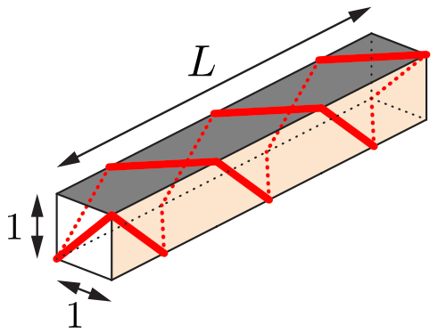
Figure 16.1: Detail from Fig. 2 in [DHK21].

For simplicity, in our version, Fig. 16.2(a), the quasigeodesic $Q$ spirals just one turn, but the example could be extended to many turns.

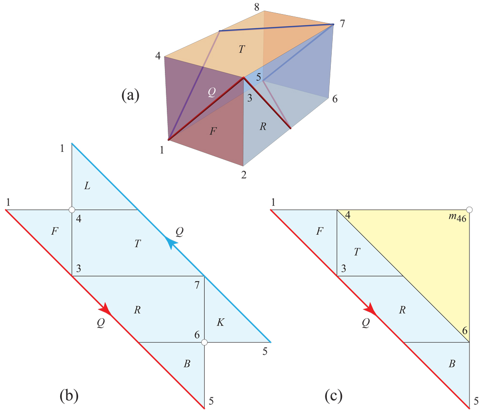
Figure 16.2: (a) A $1\times 1\times 2$ box. (b) The surface $P^{+}$ to the left of $Q$. Note the two images of $v_{1}$ are identified, as are the images of $v_{5}$. ${\omega}(v_{4})={\omega}(v_{6})=\pi/2$. (c) After merging $v_{4}$ and $v_{6}$, a cone, here flattened to a doubly-covered triangle.

Our quasigeodesic $Q=v_{1}v_{3}v_{5}v_{7}$ passes through four vertices, and encloses two vertices, $v_{4}$ and $v_{6}$, strictly to its left. Fig. 16.2(b) shows an unfolding of $P^{+}$, the half-surface left of $Q$. $P^{-}$ (not shown) is symmetrical to the right of $Q$.

Merging the two vertices $v_{4}$ and $v_{6}$ produces a cone apexed at the merge vertex $m_{46}$. For display purposes, it is flattened to the plane as a doubly-covered triangle in (c) of the figure. One can see that the portion of $P$ to the left of $Q$ is indeed a simple geodesic polygon, as claimed by Lemma 16.1.

Merging $v_{2}$ and $v_{8}$ on $P^{-}$ produces a second cone apexed at $m_{28}$. The two cones are glued together along $Q$, which still contains four vertices. So ${\cal U}$ is a polyhedron of $6$ vertices, an octahedron.

It is tempting to develop each cone to the plane to achieve nets of $P^{\varepsilon}$. This works in the example just presented, but not always, as we now detail.

Let ${\cal U}^{+}$ be the upper cone containing $P^{+}$. $P^{+}$ is topologically an annulus, with $\partial P^{+}=Q\cup Q^{\prime}$. Parametrize points $p(t)$ on the upper boundary $Q^{\prime}$, $t\in[0,1]$, with $p(0)=p(1)$. Define $\phi(t)$ to be the angular turn of the segment from $ap(0)$ to $ap(t)$ about the apex $a$ on the surface of ${\cal U}^{+}$ . Then with $\phi(0)=0$, we have that $\phi(1)={\alpha}$, for the segment makes one full turn to return to $p(0)$. However, it could be that if $Q^{\prime}$ spirals around the cone, intermediate positions represent turns greater than ${\alpha}$. See Fig. 16.3.

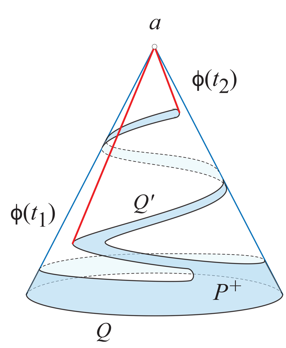
Figure 16.3: $\phi(t_{2})-\phi(t_{1})>{\alpha}$.

Let $\phi_{\max}=\max_{t_{1}<t_{2}}|\phi(t_{2})-\phi(t_{1})|$. Then $k=\lceil\phi_{\max}/{\alpha}\rceil$ represents the number of full turns around the cone that might be needed to fully develop $P^{+}$ to the plane. No overlap in the development can occur unless $k{\alpha}>2\pi$, so that the imprint of the cut-open cone cycles around $a$ more than once. Therefore we have this result.

Proposition 16.2.

If $k{\alpha}\leq 2\pi$, where $k=\lceil\phi_{\max}/{\alpha}\rceil$, then $P^{+}$ develops to the plane without overlap.

In the absence of the limit detailed in this proposition, it is indeed possible for the development of $P^{+}$ to overlap. This was established with a nontrivial example in [OV14, Fig. 14] by a curve that spirals around $a$ four times. Building this curve into $P^{+}$ would establish an overlapping development of $P^{+}$.

Another very special case occurs when ${\alpha}$ evenly divides $2\pi$. For then, even if the development spirals around $a$ more than $2\pi$, the imprint of the cut-open cone lays exactly on top of its earlier-rolled image. So any overlap in the development would have been mirrored by overlap on the cone. But $P^{+}$ does not overlap on ${\cal U}^{+}$.

Proposition 16.3.

If ${\alpha}$ evenly divides $2\pi$, then $P^{+}$ develops without overlap.

16.2.2 Reduction to Cylinder

We return now to the second option: including all vertices on $Q$ via partial merging.

Lemma 16.4.

With $P$ and $Q$ as before, let there be $k=|V(Q)|$ vertices on $Q$. Merging all vertices of $P$, along the trees $\tilde{{\Lambda}}^{\varepsilon}$, including the vertices $V$ via partial merges as described above, unfolds $P$ onto a cylinder $\cal{C}$. The unfolding of $P$ onto $\cal{C}$ is the union of at most $k-2$ simple geodesic polygons, joined circularly at $k-2$ vertices of $Q$.

Proof.

The reason the final surface is a cylinder is that (a) all vertices are merged; none remain, and (b) the curvature to each side is exactly $2\pi$: Eq. 16.1. Although Theorem 11.5 again guarantees the $P$ unfolding to each side of $Q$ is a simple geodesic polygon, as we’ve seen, the coinciding leaves of $\tilde{{\Lambda}}^{\varepsilon}$ partitions $P$ into at most $k-2$ pieces. ∎

In contrast to the two-cones case, rolling the cylinder $\cal{C}$ on the plane cannot cause overlap.

We’ve already mentioned that $k=|V(Q)|=1$ is a special case of Lemma 16.1, and $k\leq 2$ plays a special role in Lemma 16.4. We highlight the latter in the following theorem.

Theorem 16.5.

Let $P$ be a convex polyhedron and $Q$ be a simple closed quasigeodesic on $P$ containing $k=|V(Q)|$ vertices. If either

1. $k\leq 2$, or

2. if the total number of non-$\pi$ angles ${\alpha}_{i}$ and ${\beta}_{i}$ (i.e., $<\pi$ angle to both sides) is at most two,

then the unfolding of $P$ onto $\cal{C}$ (Lemma 16.4) is a simple geodesic polygon. In this case, rolling $\cal{C}$ onto a plane develops $P$ to a net.

Proof.

Lemma 16.4 established the specialness of $k\leq 2$: then the unfolding of $P$ onto $\cal{C}$ is a single, simple geodesic polygon.

When either of the angles ${\alpha}_{i}$ or ${\beta}_{i}$ incident to $q_{i}$ is equal to $\pi$, there is no need to partially merge to $q_{i}$ from one side or the other. The two slit trees can have a common leaf only at a vertex $q_{i}$ having to both sides angles strictly less than $\pi$. This reduces the number of pieces from $k-2$. ∎

Returning to Fig. 16.6 with $Q=v_{1}v_{2}v_{3}v_{4}v_{5}$, ${\alpha}_{i}=\frac{2}{3}\pi$ and ${\beta}_{i}=\pi$, so there are no angles $<\pi$ to both sides, and Theorem 16.5 applies. We will indeed see below (Fig. 16.9) this leads to a net for the icosahedron.

We believe that every convex poyhedron has a a simple closed quasigeodesic containing at most one vertex, see Open Problem 18.14. If this would be true, the above result would provide vertex-merging nets for all convex polyhedra. We discuss this question of the number of vertices on a simple closed quasigeodesic in Chapter 17.

The case $k=0$ (i.e., $Q$ is a simple closed geodesic) is considered next. In this case, $P$ contains a region $R$ isometric to a cylinder; assume $R$ is maximal with respect to inclusion. Then the two boundary components of $R$ are simple closed quasigeodesics, denoted by $Q^{\varepsilon}$. We then denote by $P^{\varepsilon}$ the caps of $P$ bounded by $Q^{\varepsilon}$ outside $R$, and apply the previous considerations. Precisely, we unfold both $P^{\varepsilon}$ onto the same cylinder, which in this case contains $R$, and further roll the cylinder to obtain a net of $P$.

The case $k=0$ is also special in that we can obtain an unfolding of $P$ onto an isosceles tetrahedron (as opposed to the doubly covered triangles obtained in Lemma 16.1 for $k=1$). In this case, $Q$ is a simple closed geodesic. Then the merging processes end with two vertices of total curvature $2\pi$, to each side of $Q$. If both of those vertices (to the same side of $Q$) have curvature $\pi$, we have reached half of an isosceles tetrahedron. Otherwise, suitably choosing a partial merge between the two vertices results in one of them having curvature $\pi$, and a new merge vertex also of curvature $\pi$. Globally, we obtain $\cal{U}$ an isosceles tetrahedron, the special case of vm-irreducible surfaces. This discussion is consistent with the above argument: once we have an isosceles tetrahedron, we can obtain the cylinder by cutting open a pair of opposite edges.

Theorem 16.6.

If $P$ contains a simple closed geodesic then, unfolding it as described above provides a net.

We next provide two examples illustrating this theorem.

16.2.3 Cube Example

To illustrate Theorem 16.6, we revisit the cube example in Section 11.3 (Fig. 11.4). There we sequentially-merged three vertices on the top face, $v_{7},v_{8}$ and then $v_{5}$ with $v_{78}$, and symmetrically three on the bottom face.

Instead now we merge all four vertices on the top face, and then on the bottom face. So, for a quasigeodesic $Q$ around the middle of the cube, we are merging all vertices inside $P^{+}$, and all vertices inside $P^{-}$, leading to a cylinder.

We perform the same two initial merges on the top vertices, resulting again in $v_{578}$. Let $a=m^{\prime}_{1}$ and $b=m^{\prime}_{2}$, the two points on the top face where the geodesic segments from the merge vertices $m_{1}=v_{12}$ and $m_{2}=v_{578}$ enter the top face of the cube.

Note that the angle incident to the merge vertex $v_{578}$ is $90^{\circ}$, and the angle incident to the as-yet unmerged top vertex $v_{6}$ is $270^{\circ}$. So a merge of $v_{578}$ with $v_{6}$ would not produce a triangle pair, because the sum of their curvatures is $2\pi$. However, we can imagine a merge resulting in a pair of unbounded parallelograms. If we cut the surface along the geodesic segment $v_{6}v_{578}$ (of length $2\sqrt{2}$ for a unit cube) and insert twin parallelograms, the result is a cylinder unbounded above. See Fig. 16.4. Note the two $45^{\circ}$ angles inserted at $v_{6}$ flattens that vertex, and the insertion of the two $135^{\circ}$ angles flattens $v_{578}$. Symmetric merges on the bottom-face vertices leads to an unbounded cylinder in both directions.

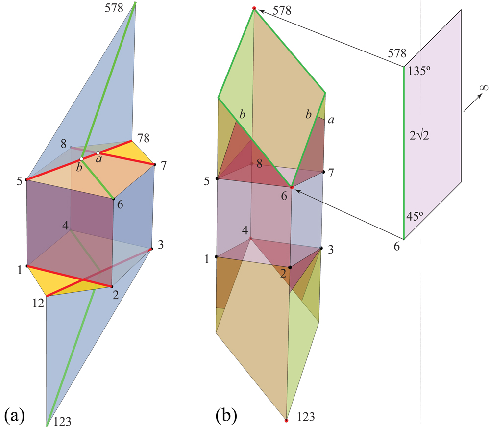
Figure 16.4: (a) Cutting along the $v_{6}v_{578}$ geodesic segment (green), and inserting double parallelograms (b) leads to an unbounded cylinder above, and similarly below. In (b) the yellow regions are inserted merge triangles; pink regions pieces of the top and bottom cube faces.

Unrolling the cylinder unfolds the cube to a non-overlapping net: Fig. 16.5.

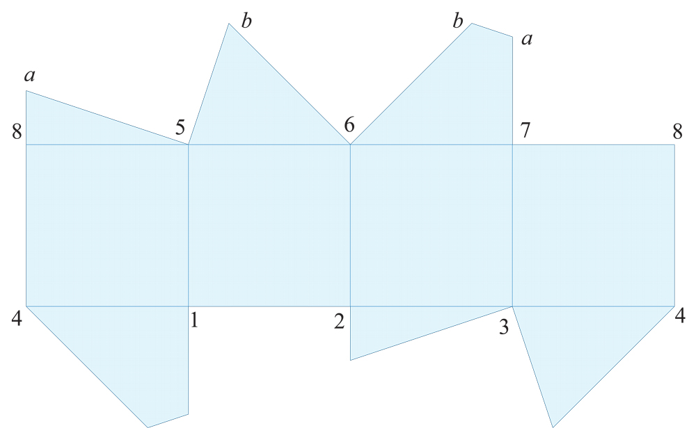
Figure 16.5: Unfolding of cube to a net by rolling the cylinder on the plane.

16.2.4 Icosahedron Example

For a second example of Theorem 16.6, we revisit and continue the example of the icosahedron from Sections 11.4 and 15.2. Fig. 16.6 below repeats for easy reference Fig. 15.2(a) showing the cuts $\tilde{g}_{i}$.

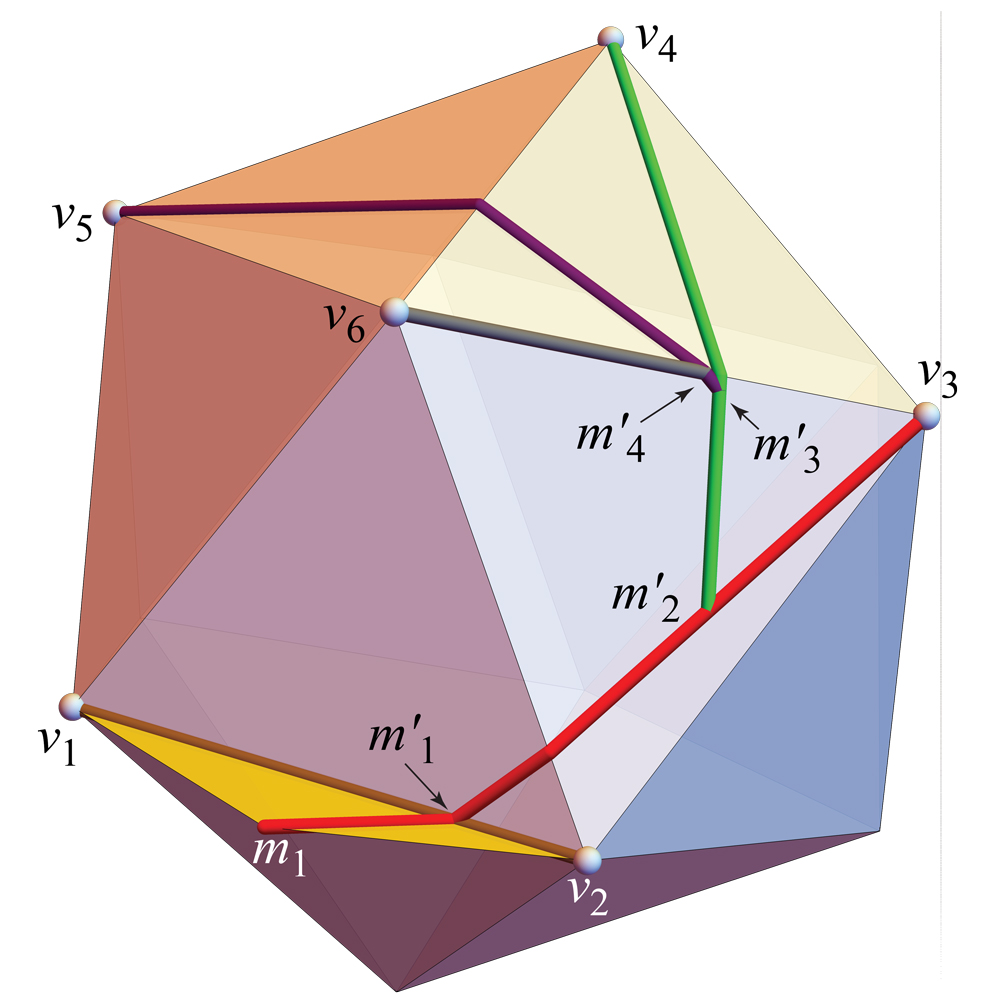
Figure 16.6: The vertex-merge cuts on $P$. Repeat of Fig. 15.2(a).

The triangles inserts $T_{1},T_{2},T_{3},T_{4}$ are shown in Fig. 16.7. Note the half angles at the merge vertex $m_{i}$ apexes of the triangles are $120^{\circ},90^{\circ},60^{\circ},30^{\circ}$ respectively. The fifth merge vertex $m_{5}$ would have zero angle, and represents the infinite parallelogram that sends $m_{5}$ to infinity.

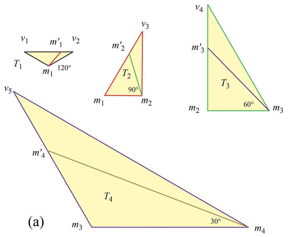
Figure 16.7: The four triangles $T_{i}$. Each is doubled to $T^{2}_{i}$ and inserted along $g_{i}$.

Inserting the doubled triangles $T^{2}_{i}$ along the cuts $g_{i}$ produces the layout shown in Fig. 16.8. Here we only show the top half of the icosahedron.

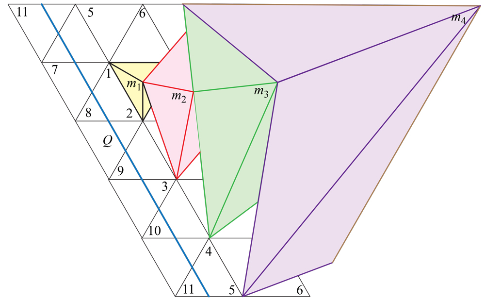
Figure 16.8: Unfolding of the top half of the icoshedron with $T^{2}_{i}$ inserted (shaded polygonal domains), $i=1,2,3,4$. Icosahedron faces are white; $Q$ is blue.

The assembly closes to a half-cylinder shown in Fig. 16.9. The infinite parallelogram $T_{5}$ with angles $60^{\circ}$ and $120^{\circ}$ (not shown) would attach at $v_{6}$ and $m_{4}$ respectively.

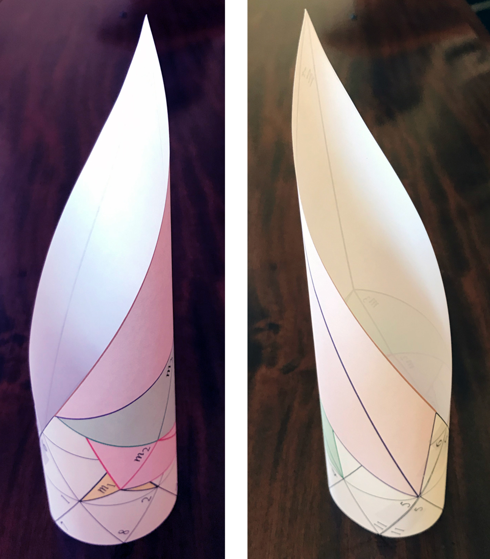
Figure 16.9: The half-cylinder obtained from Fig. 16.8 by joining the two images of $v_{11}v_{5}v_{6}$.

Joining the two symmetric half-cylinders together and rolling on the plane produces a net for the icosahedron, the white faces in Fig. 16.8.

Earlier we discussed the quasigeodesic $v_{1}v_{2}v_{3}v_{4}v_{5}$, call it $Q^{\prime}$. Note that $Q^{\prime}$ can be viewed as the $Q$ in Fig. 16.8 slid upward parallel to itself until it touches those vertices. So both lead to the same embedding on the cylinder $\cal{C}$.

Chapter 17 Vertices on Quasigeodesics

Theorem 16.5 demonstrated the importance in our context of the number of vertices on a quasigeodesic. If, as we conjecture in Open Problem 18.14, every convex polyhedron $P$ has a quasigeodesic $Q$ containing at most one vertex, then the vertex-merging described in that theorem leads to an unfolding of $P$ to a cylinder $\cal{C}$ and then to a net for $P$. In this chapter, we prove that the space ${\cal P}_{n}$ of convex polyhedra of $n$ vertices contains infinitely many polyhedra with quasigeodesics through one or two vertices, or in fact through any number $k$ of vertices, $1\leq k\leq n$. “Infinitely many” is expressed as a set in ${\cal P}_{n}$ with non-empty interior. Precise definitions are given below.

17.1 Notation

We continue to use $P$ for a convex polyhedron and $Q$ for a quasigeodesic. As in the previous chapter, $V(Q)=\{q_{1},\ldots,q_{k}\}$ is the set of vertices on $Q$; hence $k=|V(Q)|$. The spaces of polyhedra are defined as follows:

• For any $n\in{\mathbb{N}}$, let ${\cal P}_{n}$ be the space of all convex polyhedra in ${\mathbb{R}^{3}}$ with $n$ vertices, with the topology induced by the usual Pompeiu-Hausdorff metric. Two polyhedra in ${\cal P}$ are then close to each other if and only if they have close respective vertices. (See Chapter 9.)

• For all $0\leq k\leq n$, ${\cal Q}_{k}={\cal Q}_{k}(n)$ denotes the subset of ${\cal P}_{n}$ such that every $P\in{\cal Q}_{k}$ has a simple closed quasigeodesic $Q$ through exactly $k$ vertices.

17.2 ${\cal Q}_{k}$ Theorem

The goal of this chapter is to prove the following result.

Theorem 17.1.

1. ${\cal Q}_{0}$ has empty interior in ${\cal P}_{n}$.

2. ${\cal Q}_{k}$ has non-empty interior in ${\cal P}_{n}$, for all $1\leq k\leq n$.

If our conjecture in Open Problem 18.14 is true, then ${\cal Q}_{0}\cup{\cal Q}_{1}={\cal P}_{n}$.

It is not surprising that ${\cal Q}_{0}$ is rare, as it requires a partition of vertex curvatures into two halves of exactly $2\pi$ each. Indeed, (1) is a known result [Gru91], [Gal03]. As far as we are aware, (2) is new.

The proof of the second part of Theorem 17.1 will follow directly from several lemmas. Our approach is to identify a polyhedron $P$ in ${\cal Q}_{k}$ for each $k$, and then “fatten” $P$ via the next lemma.

Lemma 17.2.

Assume the convex polyhedron $P$ has a simple closed quasigeodesic $Q$ with $|V(Q)|=k\geq 1$ and

$${\alpha}_{i}<\pi,\>\>{\beta}_{i}<\pi,\>\>\forall\,1\leq i\leq k. \ast$$ ()

Then, all polyhedra $P^{\prime}$ sufficiently close to $P$ in ${\cal P}_{n}$ have such a quasigeodesic.

Proof.

The complete angles at the vertices of $P$ depend continuously on the vertex positions in ${\mathbb{R}^{3}}$. Also, the geoarcs between two vertices remain separated from other vertices by positive distances, so they also depend continuously on the vertex positions, for small perturbations of the vertices of $P$. Therefore, the strict inequalities ${\alpha}_{i}<\pi$, ${\beta}_{i}<\pi$ everywhere also remain strict for small perturbations of the vertices of $P$.

In other words, there exists a neighborhood of $P$, such that each polyhedron $P^{\prime}$ in this neighborhood still has a quasigeodesic $Q^{\prime}$ with the same number of vertices as $Q$: $|V(Q)|=|V(Q^{\prime})|$. And this is true for all $Q$ on $P$. ∎

In view of Lemma 17.2, in order to prove the second part of Theorem 17.1, it suffices to find examples of polyhedra of $n$ vertices with $Q$ satisfying $|V(Q)|=k$ and Eq. ($\ast$ ‣ 17.2), for each $1\leq k\leq n$.

17.2.1 $|V(Q)|=1$

Following the plan just articulated, we will identify doubly-covered convex polygons in ${\cal Q}_{1}$, and then apply Lemma 17.2.

Recall that the width of a convex polygon $P$ is the shortest distance between parallel supporting lines. The characterization (a) in the lemma below has long been known. We also need (b), which we could not find in the literature.

Lemma 17.3.

The width of $P$ is always achieved by (a) one of the supporting lines flush with an edge $e$ of $P$, and (b) the other line including a vertex that projects onto $e$.

Proof.

Claim (a) is Theorem 2.1 in [HT88], and known earlier. Their proof uses a lemma (their Lemma 2.1) that says the following. Let $u$ and $v$ be two points in the plane, and parallel lines $L_{u}$ and $L_{v}$ through each respectively. Then there exists a “preferred direction of rotation” of the lines, maintaining parallelism and maintaining contact with $u$ and $v$, that diminishes the separation between the lines. They call this the PDR lemma. In the special case when the lines are orthogonal to $vu$, then both directions of rotation reduce separation.

Claim (b) relies on this PDR lemma. But as they skip proving their lemma, we include a proof here. Let $ab=e$ be the edge of $P$ with supporting line $L_{ab}$ including $e$. Let the parallel line be $L_{c}$, including only vertex $c$, with the separation between the lines width $w$. Assume, in contradiction to claim (b), that $c$ does not project onto $ab$. The situation is then as depicted in Fig. 17.1, with $ac$ playing the role of $uv$ in the PDR lemma.

Rotate $L_{ab}$ and $L_{c}$ about $a$, clockwise in the figure—this is the preferred direction. Then $L_{c}$ pivots around point $p$, and is no longer supporting $P$. Now move it (down in the figure) until it again contacts $c$. Call the new lines $L^{\prime}_{ab}$ (red) and $L^{\prime}_{c}$ (green), and let $w^{\prime}$ be their separation. Note that $h^{2}=w^{2}+x^{2}$, and $h^{2}=(w^{\prime})^{2}+(x^{\prime})^{2}$. The rotation ensures that $x^{\prime}>x$, and therefore $w^{\prime}<w$, contradicting the assumption that the width is $w$.

If $c$ instead does project into $ab$, as per claim (b), say to point $q\in ab$, then the line $L_{ab}$ is blocked from the preferred direction of rotation because it would penetrate $P$ at $q$.

If $c$ is the endpoint of an edge $cd$ parallel to $ab$, then at least one of the four vertices $\{a,b,c,d\}$ must project onto the opposite edge, so claim (b) holds. ∎

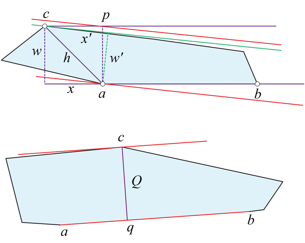
Figure 17.1: (a) Vertex $c$ projects outside $ab$. (b) $cq$ realizes the width.

Lemma 17.4.

Every doubly-covered convex polygon $P$ with no parallel edges has a quasigeodesic through one vertex.

Proof.

Let $Q$ be the segment from a vertex $c$ orthogonal to an edge $ab$ at a point $q$, as guaranteed by Lemma 17.3 and illustrated in Fig. 17.1(b). The angles on the doubled polygon at $q$ are both $\pi$, and the left and right angles at $c$ are both $<\pi$ (strictly less than because of the no-parallel-edges assumption). Therefore $Q=cq$ is a quasigeodesic.

If $q=a$, i.e., if $c$ projects to an endpoint of $ab$, then the PDR lemma shows that $c$ and $ab$ could not have realized the width; see Fig. 17.2(a). Both directions of rotation diminish the separation, with one direction blocked by the flush edge. Therefore, $q$ must project into the interior of $ab$, and $Q$ includes just the one vertex $c$. ∎

Although not needed for Theorem 17.1, for completeness we also handle parallel edges.

Lemma 17.5.

If the width of a convex polygon $P$ is achieved on parallel edges, then the doubly covered $P$ has a simple closed geodesic.

Proof.

Let the width of $P$ be realized by edges $ab$ and $cd$. If the projection of $cd$ onto $ab$ is a positive-width interval, then a closed geodesic can be achieved by a pair of points, one on each edge, strictly interior to this interval.

If instead the projection interval is a point, then that point corresponds to a vertex-to-vertex projection, say $c$ to $b$ in Fig. 17.2(b). But in this circumstance, again the PDR lemma shows that $|cb|$ cannot have been the width, as rotation of the supporting lines toward the $<\pi/2$ side of $b$ and $c$ (counterclockwise in the figure) reduces the separation between the lines. ∎

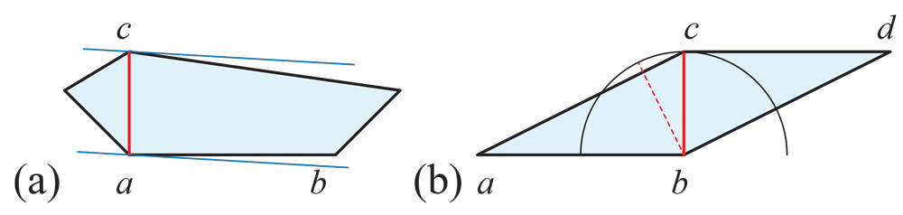
Figure 17.2: Neither $ca$ (a) nor $bc$ (b) realizes the width.

Note that the previous two lemmas together ensure that every doubly-covered convex polygon has a quasigeodesic through at most one vertex.

The following lemma is not needed for our main goal, but might possibly help in resolving Open Problem 18.14.

Lemma 17.6.

The width-quasigeodesic identified in Lemmas 17.4–17.5 is the shortest quasigeodesic for $P$.

Proof.

Call the width-quasigeodesic $Q_{w}$, and the width $w$. So $\ell(Q_{w})=2w$. First we show there is no shorter $1$-vertex quasigeodesic. Suppose $Q$ were such a quasigeodesic through $v$. It must be orthogonal to an edge $e$ of $P$, and then the line parallel to $e$ through $v$ is a supporting line for $P$. Therefore, if $Q$ were shorter than $Q_{w}$, the width of $P$ would not be $w$.

Suppose now there is a shorter diagonal-quasigeodesic, connecting vertices $a$ and $b$. Then lines orthogonal to $ab$ through $a$ and $b$ must be supporting lines, to satisfy the angle constraints needed for the quasigeodesic to be convex to both sides at $a$ and $b$. This again would contradict $Q_{w}$ realizing the width.

A $0$-vertex quasigeodesic $Q$ must cross parallel edges of $P$. It could be slid left or right until it touches a vertex, in which case it is now a $1$-vertex quasigeodesic, and the argument above applies. ∎

17.2.2 $|V(Q)|=2$

Lemma 17.7.

Every doubly covered polygon has a simple closed quasigeodesic $Q$ with $|V(Q)|=2$

Proof.

Each extrinsic diameter of a convex polyhedron $P$,

$$\mathrm{diam}\left(P\right):=\max_{x,y\in P}|x-y|,$$

is realized between two vertices of $P$, see for example Proposition 1 in [IRV20]. Because of its length maximality, such a diameter provides, for doubly covered polygons, the desired quasigeodesics through $2$ vertices. ∎

17.2.3 $|V(Q)|=k$, with $3\leq k\leq n$

For these cases, we construct particular examples of polyhedra $P_{n}$ of $n$ vertices each of which has at least one quasigeodesic through $k$ vertices.

Lemma 17.8.

For every $3\leq k\leq n$ there exist doubly covered $n$-gons having simple closed quasigeodesics $Q_{k}$ with $|V(Q_{k})|=k$ and satisfying Eq. ($\ast$ ‣ 17.2).

Proof.

Consider a regular $k$-gon $R_{k}=v_{1}\ldots v_{k}$, where $3\leq k\leq n$. Figure 17.3 illustrates the case $k=6$.

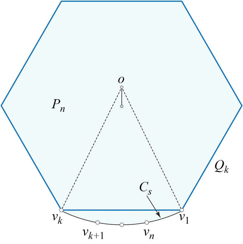
Figure 17.3: $Q_{6}$ is the blue hexagon. $C_{s}$ is centered at $o$ above the hexagon center.

Also consider the circle $C$ through $v_{1}$ and $v_{k}$, of centre $o$ on the same side of $v_{1}v_{k}$ as $R_{k}$. On the short arc $C_{s}$ of $C$ determined by $v_{1}$ and $v_{k}$, choose points $v_{k+1},\ldots,v_{n}$, to increase the polygon to $n$ vertices, and denote by $P_{n}$ the doubly covered polygon $v_{1}\ldots v_{n},v_{1}$.

When the center $o$ is beyond the center of $R_{k}$ as illustrated, the measure (length) of $m(C_{s})$ satisfies $m(C_{s})<2\pi/k$. It follows that $P_{n}$ has two simple closed quasigeodesics $Q_{k}$ with $k$ vertices, both corresponding to the polygon $v_{1}\ldots v_{k},v_{1}$, one including edge $v_{1}v_{k}$ on the front, and one on the back.

Indeed, for $Q_{k}$

• the angles ${\alpha}_{i}$ are each the vertex angles of $R_{k}$, equal to $\frac{(k-2)}{k}\pi<\pi$, for $1\leq i\leq k$.

• the angles ${\beta}_{i}={\alpha}_{i}$ for $1<i<k$.

• For $i=1$, ${\beta}_{1}$ is ${\alpha}_{1}$ plus twice $\angle v_{k}v_{1}v_{n}$, and $\angle v_{k}v_{1}v_{n}<m(C_{s})/2$. Similarly for $i=k$. Therefore, for $i\in\{1,k\}$,

  $${\beta}_{i}<{\alpha}_{i}+m(C_{s})<\frac{k-2}{k}\pi+\frac{2}{k}\pi<\pi\;.$$

Thus $Q_{k}$ is a quasigeodesic satisfying Eq. ($\ast$ ‣ 17.2) of Lemma 17.2. ∎

Returning to Theorem 17.1, we have identified polygons with $|V(Q)|=k$, for $1\leq k\leq n$, and applying Lemma 17.2 creates ${\cal Q}_{k}$ with nonempty interiors. This establishes Theorem 17.1.

Chapter 18 Conclusions
and Open Problems

Our work leaves open several questions of various natures, most of which have been mentioned in the text in some form. Here we list open problems and indicate possible directions for future research. The exposition roughly follows the order we treated the subjects, with the comments on both parts joined in this final chapter.

18.1 Part I

In the first part of this work, we mainly studied properties of the tailoring operation on convex polyhedra.

• We have presented three methods for tailoring, of very different flavors. On one hand, the methods of tailoring with sculpting given in Chapters 4 and 7—digon-tailoring or crest-tailoring—seem appropriate for local tailoring, and can produce any $Q$ inside $P$.

  On the other hand, the method of tailoring via flattening presented in Chapter 8 is purely intrinsic, in that it doesn’t need the spatial structure of $P$ and $Q$ to work. The surfaces can be given, in this case, as a collection of polygons glued together as in AGT. But it has the disadvantage of being “non-economical,” in the sense that it discards a lot of $P$’s surface area.

  Even with “surface-removal optimal” tailoring, we could be forced to lose almost all the surface area of $P$ to reshape to $Q$, for example if approximating by tailoring a sphere inscribed in a very long convex surface.

  All three methods can be reversed to enlarge surfaces, where the results are the same, but not-requiring the spatial structure might be a clear advantage.

• We made little attempt to optimize our algorithm complexities, resting content with polynomial-time upper bounds. Likely several algorithms could be improved, or lower bounds established. Especially notable is this problem, which dominates the complexity of the tailoring-via-flattening algorithm, Theorem 8.3.

  Open Problem 18.1.

  Given a polyhedron $P$ of $n$ vertices, find a cut-locus generic point $x$ in less than $O(n^{4})$ time.

  Such a generic point has a unique geodesic segment (shortest path) to each vertex of $P$.

• Recall that Lemma 4.1 established that, with a slice along the plane of a face $X$ of $Q\subset P$, the portion of $P$ sliced-off can be partitioned into a fan of g-domes. Then Theorem 3.2 showed how to reduce a g-dome to its base by removing pyramids.

  Rather than repeating this for each face $X$ of $Q$, it is conceivable that a single base $X$ and a single g-dome suffice.

  Open Problem 18.2.

  Let $X$ be a “base” face of $P$, and $D$ a fixed g-dome over $X$, interior to $P$. Is it possible to partition $P$ into pyramids and $D$, with planes through the edges of $X$? After each sectioning we remove the sliced pyramid.

  If g-dome $D$ is replaced with an arbitrary interior polyhedron, then the answer is easily seen to be no. Without the restriction to planes through base edges, the answer is yes as shown by Lemma 4.1.

• As discussed in Section 5.5.1, the proof of Theorem 5.3—that the seal graph ${\Sigma}$ for a pyramid is a tree—depends on the ordering of digon removal.

  Open Problem 18.3.

  Is the seal graph for a pyramid a tree for other orderings of digon removal?

• We have shown in Chapter 9 that different unfoldings of $Q\subset P$ onto $P$ exist. Clearly, the $P$-unfolding obtained via tailoring depends on the order of tailoring operations. The $P$-unfolding of $Q$ does not necessarily have connected interior, which suggests this problem:

  Open Problem 18.4.

  Is there some method and/or orderings of tailoring operations that would render interior-connected a $P$-unfolding of arbitrary $Q\subset P$? A less ambitious goal would be to minimize the number of interior-connected pieces.

  Notice that Theorem 9.3 established simply connectedness in general. But in our usage, simply connected does not imply connected, e.g., the union of several disjoint disks is a disconnected set but simply connected. In Part II we pursue this question for particular $P$, for example, a doubly-covered triangle.

• Theorem 9.5 established the existence of a continuous folding of $P$ onto $Q$ when $Q\subset P$, but we do not know of an algorithm:

  Open Problem 18.5.

  Is there a finite algorithm that determines a continuous unfolding of $P$ onto $Q$?

• It seems that at least a part of the present work could apply to $1$-polyhedra. These are polyhedra whose faces are (congruent to) geodesic polygons on the unit sphere. They can approximate convex surfaces with curvature bounded below by $1$ (in the sense of A. D. Alexandrov), just as convex polyhedra can approximate ordinary convex surfaces [AZ67], [IRV15].

  Open Problem 18.6.

  How much of the presented results can be carried over and applied to $1$-polyhedra?

• One could also define tailoring for general (i.e., not necessarily convex) polyhedra, of arbitrary topology. Of course, the methods we developed here apply locally to convex caps. Globally, a necessary condition for $Q$ to be tailored from a homothetic copy of $P$ is to have the same topology as $P$. Our Theorem 4.6 might suggest this is also sufficient, but that is not true. By Alexandrov’s Gluing Theorem (AGT), tailoring a convex polyhedron always produces a convex polyhedron, never a nonconvex polyhedron homeomorphic to the sphere but having negative curvature at some vertex. There is as yet no counterpart to AGT for nonconvex polyhedra. Therefore, in the general framework, tailoring could be a much subtler topic.

  Open Problem 18.7.

  Is there a type of tailoring operation that permits global reshaping of non-convex polyhedra?

18.2 Part II

In the second part of this work, we mainly studied the vertex-merging (as opposed to tailoring) processes on convex polyhedra, with the aim of producing “nice” polyhedral and planar unfoldings. Toward that aim, we needed to develop a theory of convex sets on convex polyhedra.

• For any convex polyhedron $P$, there clearly exist vertex-merging reductions of $P$ that increase the surface area by the least, or the most amount.

  Open Problem 18.8.

  Find upper and lower bounds on the added surface area for vertex-merging reductions of $P$. Find the reduction yielding the minimal, and respectively maximal area.

• General relationships between the properties of the slit graph and those of the corresponding unfolding of $P$ are presented in Theorem 11.5. Finding particular vertex-mergings with “good” behaviour seems to be a difficult task, only partly fulfilled in this study.

  Open Problem 18.9.

  Does there exist for every convex polyhedron $P$ a vertex-merging reduction onto a vm-irreducible surface whose slit graph has no cycle? If not, for which $P$ are there such vm-reductions?

• A positive answer to the above question raises another one, related to our discussion in Section 11.7.

  Open Problem 18.10.

  For any simple unfolding $P_{S}$ of $P$ onto a vm-irreducible surface $S$, does there exists an unfolding of $S$ in the plane which results in a net for $P$?

• Our attempt to answer Open Problem 18.9 is based on a spiral-merging idea. In order to formalize our spiraling algorithms, we needed to develop a theory of convex sets on convex polyhedra. We only proved some basic results in this theory, and much remains for future study. In particular, the next question is related to Lemma 13.14 for the case when $S\supseteq Q$.

  Open Problem 18.11.

  Is it the case that every closed convex subset $S$ of a convex polyhedron is either included in a half-surface bounded by a simple closed quasigeodesic $Q$, or is the whole surface?

• Of the classical results in the combinatorial theory of convex sets bearing a name, we only adapted to our framework the Krein–Milman Theorem (that a convex set is the convex hull of its extreme points); see Theorem 13.32. Perhaps the statement of that result, even though suitable to our purpose, could be improved.

  Open Problem 18.12.

  Is Theorem 13.32 concerning extreme points and the relative convex hull, still true without the “relative” modifier?

• Examples 13.13 and 13.22 show that the precise planar versions of Helly’s and Radon’s theorems are false on the surface of a convex polyhedron. It seems worth studying if there are versions of these theorems, and of Carathéodory’s theorem, in our context.

  Open Problem 18.13.

  Are there versions of Helly’s, Radon’s, and Carathéodory’s theorems that hold on the surface of a convex polyhedron, using ag-convexity?

  The Radon point of any four points in the plane is their geometric median, the point that minimizes the sum of distances to the other points [CEM⁺96]. Therefore, it could also be of some interest to study such points in our framework. Note, for example, on a doubly covered square there are two such points, the centers of the two faces.

• Theorem 16.5 established that if a polyhedron $P$ has a quasigeodesic including at most two vertices, vm-reduction can lead to a net for $P$. One might view the reduction process as moving $P$ closer and closer to planarity, as $P_{i}$ has fewer and fewer vertices. Finally $P$ is on a cylinder which rolls to a net.

  Little seems known about the structure of quasigeodesics. Pogorelov’s original proof is nonconstructive [Pog49], [Pog73], and it has long been an open problem to design an algorithm to find a simple closed quasigeodesic (Open Problem 24.2 [DO07]). It is not difficult to find a plane $\Pi$ through one vertex whose slice curve $C=\Pi\cap P$ halves the curvature as needed. But $C$ is not necessarily convex [O’R03], and so in general is not a quasigeodesic.

  However, there has been recent progress on quasigeodesics. First, a pseuopolynomial-time algorithm was designed that finds a possibly self-crossing quasigeodesic [KPD09]. Second, an exponential algorithm for finding all the simple closed quasigeodesics was described in [CdM22]. Despite this progress, there remains no practical algorithm for finding simple closed quasigeodesics.

  Open Problem 18.14.

  We conjecture that every convex polyhedron either has a simple closed geodesic, or a simple closed quasigeodesic through just one vertex.

  Note that this conjecture is verified for doubly-covered convex polygons, by Lemmas 17.4 and 17.5. We recently proved the conjecture for tetrahedra [OV22].

Bibliography

- [AAC+12] Timothy G. Abbott, Zachary Abel, David Charlton, Erik D. Demaine, Martin L. Demaine, and Scott Duke Kominers. Hinged dissections exist. Discrete Comput. Geom., 47(1):150–186, 2012.
- [AAOS97] Pankaj K. Agarwal, Boris Aronov, Joseph O’Rourke, and Catherine A. Schevon. Star unfolding of a polytope with applications. SIAM J. Comput., 26:1689–1713, 1997.
- [ADD+14] Zachary Abel, Erik D Demaine, Martin L Demaine, Jin-ichi Itoh, Anna Lubiw, Chie Nara, and Joseph O’Rourke. Continuously flattening polyhedra using straight skeletons. In Proc. 30th Ann. Symp. Comput. Geom., pages 396–405, 2014.
- [ADD+21] Zachary Abel, Erik D. Demaine, Martin L. Demaine, Jason S. Ku, Jayson Lynch, Jin ichi Itoh, and Chie Nara. Continuous flattening of all polyhedral manifolds using countably infinite creases. Comput. Geom.: Th. Appl., 2021. To appear. https://arxiv.org/abs/2105.10774.
- [ADO03] Rebecca Alexander, Heather Dyson, and Joseph O’Rourke. The convex polyhedra foldable from a square. In Proc. 2002 Japan Conf. Discrete Comput. Geom., volume 2866 of Lecture Notes in Comput. Sci., pages 38–50. Springer-Verlag, 2003.
- [AKP19] Stephanie Alexander, Vitali Kapovitch, and Anton Petrunin. Alexandrov geometry: Preliminary version no. 1. arXiv:1903.08539, 2019.
- [Ale78] Stephanie Alexander. Local and global convexity in complete Riemannian manifolds. Pacific J. Math., 76(2):283–289, 1978.
- [Ale05] Aleksandr D. Alexandrov. Convex Polyhedra. Springer-Verlag, Berlin, 2005. Monographs in Mathematics. Translation of the 1950 Russian edition by N. S. Dairbekov, S. S. Kutateladze, and A. B. Sossinsky.
- [ALT12] Paul T. Allen, Adam Layne, and Katharine Tsukahara. The dirichlet problem for curve shortening flow. arXiv preprint arXiv:1208.3510, 2012.
- [ALZ20] Elena Arseneva, Stefan Langerman, and Boris Zolotov. A complete list of all convex polyhedra made by gluing regular pentagons. J. Info. Processing, 28:791–799, 2020.
- [AN19] Sergey Avvakumov and Gabriel Nivasch. Homotopic curve shortening and the affine curve-shortening flow. arXiv preprint arXiv:1909.00263, 2019.
- [AO92] Boris Aronov and Joseph O’Rourke. Nonoverlap of the star unfolding. Discrete Comput. Geom., 8:219–250, 1992.
- [AS05] Pankaj K. Agarwal and Micha Sharir. Pseudo-line arrangements: Duality, algorithms, and applications. SIAM J. Comput., 34(3):526–552, 2005.
- [AZ67] Aleksandr D. Alexandrov and Victor A. Zalgaller. Intrinsic Geometry of Surfaces. American Mathematical Society, Providence, RI, 1967.
- [Ban81] Victor Bangert. Totally convex sets in complete Riemannian manifolds. J. Differential Geom., 16(2):333–345, 1981.
- [BI08] Alexander I. Bobenko and Ivan Izmestiev. Alexandrov’s theorem, weighted Delaunay triangulations, and mixed volumes. Ann. Inst. Fourier (Grenoble), 58(2):447–505, 2008.
- [BZ21] Thomas Bendokat and Ralf Zimmermann. Efficient quasi-geodesics on the Stiefel manifold. arXiv:2105.07017, 2021.
- [CdM22] Jean Chartier and Arnaud de Mesmay. Finding weakly simple closed quasigeodesics on polyhedral spheres. To appear, Symp. Comput. Geom., June 2022.
- [CEG+93] Bernard Chazelle, Herbert Edelsbrunner, Leonidas Guibas, Micha Sharir, and Jack Snoeyink. Computing a face in an arrangement of line segments and related problems. SIAM J. Comput., 22(6):1286–1302, 1993.
- [CEM+96] Kenneth L. Clarkson, David Eppstein, Gary L. Miller, Carl Sturtivant, and Shang-Hua Teng. Approximating center points with iterative Radon points. Internat. J. Comput. Geom. Appl., 6(03):357–377, 1996.
- [CH90] Jindong Chen and Yijie Han. Shortest paths on a polyhedron. In Proc. 6th Ann. Symp. Comput. Geom., pages 360–369, 1990.
- [CH96] Jindong Chen and Yijie Han. Shortest paths on a polyhedron, Part I: Computing shortest paths. Internat. J. Comput. Geom. Appl., 6(02):127–144, 1996.
- [CSW99] Francis Chin, Jack Snoeyink, and Cao An Wang. Finding the medial axis of a simple polygon in linear time. Discrete Comput. Geom., 21(3):405–420, 1999.
- [DEE+03] Erik D. Demaine, David Eppstein, Jeff Erickson, George W. Hart, and Joseph O’Rourke. Vertex-unfoldings of simplicial manifolds. In A. Bezdek, editor, Discrete Geometry, pages 215–228. Marcel Dekker, 2003.
- [DHK21] Erik D. Demaine, Adam C. Hesterberg, and Jason S. Ku. Finding closed quasigeodesics on convex polyhedra. Discrete Comput. Geom., 2021. arXiv:2008.00589. SoCG2020. To appear Discrete Comput. Geom.
- [DO07] Erik D. Demaine and Joseph O’Rourke. Geometric Folding Algorithms: Linkages, Origami, Polyhedra. Cambridge University Press, 2007. http://www.gfalop.org.
- [EHPN20] David Eppstein, Sariel Har-Peled, and Gabriel Nivasch. Grid peeling and the affine curve-shortening flow. Exp. Math., 29(3):306–316, 2020.
- [EL13] David Eppstein and Maarten Löffler. Bounds on the complexity of halfspace intersections when the bounded faces have small dimension. Discrete Comput. Geom., 50(1):1–21, 2013.
- [Epp20] David Eppstein. Treetopes and their graphs. Discrete Comput. Geom., pages 1–31, 2020.
- [Gal03] Gregorii Aleksandrovich Gal’perin. Convex polyhedra without simple closed geodesics. Regul. Chaotic Dyn., 8(1):45–58, 2003.
- [GM01] Clara I. Grima and Alberto Márquez. Computational Geometry on Surfaces. Kluwer Academic, Dordrecht, 2001.
- [Gru91] Peter Gruber. A typical convex surface contains no closed geodesic. J. Reine Angew. Math., 416:195–205, 1991.
- [HT88] Michael E. Houle and Godfried T. Toussaint. Computing the width of a set. IEEE Trans. Pattern Anal. Mach. Intell., 10(5):761–765, 1988.
- [IN10] Jin-ichi Itoh and Chie Nara. Continuous flattening of Platonic polyhedra. In Internat. Conf. Comput. Geometry, Graphs and Applications, pages 108–121. Springer, 2010.
- [INV12] Jin-ichi Itoh, Chie Nara, and Costin Vîlcu. Continuous flattening of convex polyhedra. In Computational Geometry, volume 7579, pages 85–97. Lecture Notes in Comput. Sci., 2012.
- [IRV15] Jin-ichi Itoh, Joël Rouyer, and Costin Vîlcu. Moderate smoothness of most alexandrov surfaces. Internat. J. Math., 26(04):1540004, 2015.
- [IRV20] Jin-ichi Itoh, Joël Rouyer, and Costin Vîlcu. Some inequalities for tetrahedra. Beitr. Algebra Geom., pages 1–11, 2020. https://doi.org/10.1007/s13366-020-00549-w.
- [KPD09] Daniel Kane, Gregory N. Price, and Erik D. Demaine. A pseudopolynomial algorithm for Alexandrov’s theorem. In Workshop Algorithms Data Struct., pages 435–446. Springer, 2009.
- [LP21] Alexander Lytchak and Anton Petrunin. About every convex set in any generic Riemannian manifold. arXiv:2103.15189, 2021.
- [Meg83] Nimrod Megiddo. Linear-time algorithms for linear programming in and related problems. SIAM J. Comput., 12(4):759–776, 1983.
- [Mit16] Octavian Mitrea. Geodesic convexity types in Riemannian manifolds. arXiv:1611.08643, 2016.
- [O’R01] Joseph O’Rourke. An extension of Cauchy’s arm lemma with application to curve development. In Proc. 2000 Japan Conf. Discrete Comput. Geom., volume 2098 of Lecture Notes in Comput. Sci., pages 280–291. Springer-Verlag, 2001.
- [O’R03] Joseph O’Rourke. On the development of the intersection of a plane with a polytope. Comput. Geom., 24(1):3–10, 2003.
- [O’R07] Joseph O’Rourke. Computational geometry column 49. Internat. J. Comput. Geom. Appl., 38(2):51–55, 2007. Also in SIGACT News, 38(2): 51–55(2007), Issue 143.
- [O’R13] Joseph O’Rourke. Dürer’s problem. In Marjorie Senechal, editor, Shaping Space: Exploring Polyhedra in Nature, Art, and the Geometrical Imagination, pages 77–86. Springer, 2013.
- [O’R20] Joseph O’Rourke. Vertex-transplants on a convex polyhedron. In Proc. 32st Canad. Conf. Comput. Geom., 2020. To appear.
- [OV14] Joseph O’Rourke and Costin Vîlcu. Conical existence of closed curves on convex polyhedra. Comput. Geom., 47:149–163, 2014.
- [OV20] Joseph O’Rourke and Costin Vîlcu. Tailoring for every body: Reshaping convex polyhedra. https://arxiv.org/abs/2008.01759, August 2020.
- [OV22] Joseph O’Rourke and Costin Vîlcu. Simple closed quasigeodesics on tetrahedra. Information, 13:238–258, May 2022.
- [Pog49] Aleksei V. Pogorelov. Quasi-geodesic lines on a convex surface. Mat. Sb., 25(62):275–306, 1949. English transl., Amer. Math. Soc. Transl. 74, 1952.
- [Pog73] Aleksei V. Pogorelov. Extrinsic Geometry of Convex Surfaces, volume 35 of Translations of Mathematical Monographs. Amer. Math. Soc., Providence, RI, 1973.
- [Poi05] Henri Poincaré. Sur les lignes géodésiques des surfaces convexes. Trans. Amer. Math. Soc., 6:237–274, 1905.
- [Rou03] Joël Rouyer. Antipodes sur un tétraedre régulier. J. Geom., 77(1-2):152–170, 2003.
- [SS86] Micha Sharir and Amir Schorr. On shortest paths in polyhedral spaces. SIAM J. Comput., 15:193–215, 1986.
- [SS08] Yevgeny Schreiber and Micha Sharir. An optimal-time algorithm for shortest paths on a convex polytope in three dimensions. Discrete Comput. Geom., pages 500–579, 2008. Twentieth Anniversary Volume.
- [Udr13] Constantin Udriste. Convex functions and optimization methods on Riemannian manifolds, volume 297. Springer Science & Business Media, 2013.
- [Vis18] Nisheeth K. Vishnoi. Geodesic convex optimization: Differentiation on manifolds, geodesics, and convexity. arXiv:1806.06373, 2018.
- [Wik21] Wikipedia. Curve-shortening flow. https://en.wikipedia.org/wiki/Curve-shortening_flow, March 2021.
- [Zal07] V. A. Zalgaller. An isoperimetric problem for tetrahedra. J. Math. Sci. (N.Y.), 140(4):511–527, 2007.
- [Zam91] Tudor Zamfirescu. Baire categories in convexity. Atti Sem. Mat. Fis. Univ. Modena, 39:139–164, 1991.