A theoretical framework of chorus wave excitation

Abstract

We propose a self-consistent theoretical framework of chorus wave excitation, which describes the evolution of the whistler fluctuation spectrum as well as the supra-thermal electron distribution function. The renormalized hot electron response is cast in the form of a Dyson-like equation, which then leads to evolution equations for nonlinear fluctuation growth and frequency shift. This approach allows us to analytically derive for the first time exactly the same expression for the chorus chirping rate originally proposed by Vomvoridis . (1982). Chorus chirping is shown to correspond to maximization of wave particle power exchange, where each individual wave belonging to the whistler wave packet is characterized by small nonlinear frequency shift. We also show that different interpretations of chorus chirping proposed in published literature have a consistent reconciliation within the present theoretical framework, which further illuminates the analogy with similar phenomena in fusion plasmas and free electron laser physics.

1 Introduction

Chorus waves are whistler mode waves with frequency ($\omega$) typically between one tenth of and the electron cyclotron frequency ($\Omega$) (see, e.g., Tsurutani  Smith, 1974; Burtis  Helliwell, 1976). These waves have been demonstrated to play important roles in energetic electron dynamics in the terrestrial magnetosphere. Chorus waves are responsible for the acceleration of a few hundred keV electrons to the MeV energy range, leading to the enhancement of MeV electron fluxes in the outer radiation belt during geomagnetically disturbed times (Horne  Thorne, 1998; Horne ., 2005; Y. Chen ., 2007; Bortnik  Thorne, 2007; Reeves ., 2013; Thorne ., 2013). Furthermore, scattering of a few hundred eV to a few keV electrons by chorus waves into the atmosphere has been shown to be the dominant process in the formation of energetic electron pancake distributions (Tao ., 2011), diffuse aurora (Thorne ., 2010), and pulsating aurora (Miyoshi ., 2010; Nishimura ., 2010).

Chorus waves consist of quasi-coherent discrete elements with frequency chirping. In the terrestrial magnetosphere, the frequency of a chorus element may vary by a few hundred Hz to a few kHz in less than a second. Previous studies have established that coherent nonlinear wave particle interactions play a key role in the frequency chirping, and have demonstrated that the chirping rate for rising tone chorus is proportional to the wave amplitude. Using a series of simulations, Vomvoridis . (1982) argued that, to maximize wave power transfer, the frequency chirping rate and the wave amplitude for parallel propagating chorus waves is related by

$$\frac{\partial\omega}{\partial t}=R\left(1-\frac{v_{r}}{v_{g}}\right)^{-2}\omega_{tr}^{2},$$ (1)

with $R=1/2$. Here $v_{r}$ is the cyclotron resonant velocity, $v_{g}$ is the wave group velocity, and $\omega_{tr}^{2}=kv_{\perp}e\delta B/(mc)$ with $v_{\perp}$ the perpendicular velocity, $k$ the wave number, and $\delta B$ the wave amplitude. Theoretical interpretation of Eq. (1) was proposed by Trakhtengerts . (2004) and Demekhov (2011), based on the assumption that a chorus element is formed as a succession of sidebands separated from each other by the trapping frequency $\omega_{tr}$ over timescales $2\pi/\omega_{tr}$. Meanwhile, for optimum cyclotron power exchange of electrons with a whistler wave in an inhomogeneous magnetic field, the growth rate is determined by a Backward Wave Oscillator (BWO) condition. Good agreement from comparisons of these chorus sweeping rate predictions with observations was reported by (Trakhtengerts ., 2004; Macúšová ., 2010; Tao ., 2012). Another interpretation of Eq. (1) was proposed by Omura . (2008), by assuming a constant value for the phase space density of phase-trapped electrons, and demonstrating that the resonant current density in the direction of wave electric field maximizes at $R=0.4$, consistent with Eq. (1) of Vomvoridis . (1982). Equation (1) has been verified by several different particle-in-cell (PIC) type simulations (Katoh  Omura, 2011, 2013; Hikishima  Omura, 2012; Tao ., 20171, 20172) and an observational study (Cully ., 2011). More recently, Mourenas . (2015) suggested using the nonlinear chorus growth rate from Shklyar  Matsumoto (2011), based on contributions from both trapped and untrapped resonant particles, to derive an analytical estimate of the value of $R=S^{*}$ maximizing this nonlinear growth rate. They obtained $R=S^{*}=3/5$ in the case of oblique chorus waves.

Despite of Eq. (1) being a huge success, its derivation was based either on simulations (Vomvoridis ., 1982) or by assuming either a given behavior of the fluctuation spectrum (Trakhtengerts ., 2004; Demekhov, 2011), or a specific form of the distribution function for phase trapped (Omura ., 2008) and/or untrapped (Shklyar  Matsumoto, 2011; Mourenas ., 2015) particles. Besides , Eq. (1) was derived assuming the pre-existence of frequency chirping (Vomvoridis ., 1982). The reason for frequency chirping of chorus was explained by Omura  Nunn (2011) due to the nonlinear current parallel to the wave magnetic field ($J_{B}$), which causes frequency shift. In this paper, we propose a new first principle based theoretical framework for chorus wave excitation that addresses the dynamic evolution of the fluctuation spectrum and its interaction with trapped as well as untrapped resonant particles on the same footing. This self-consistent analysis is a novelty of the present approach with respect to previous studies. By keeping the dominant long-term nonlinear response in the distribution function, we obtain an equation for the evolution of the distribution function of hot electrons in the form of a Dyson-like equation (Dyson, 1949; Schwinger, 1951). This model (L. Chen  Zonca, 2016; Zonca, Chen, Briguglio, Fogaccia, Vlad  Wang, 2015) explains chirping as a result of the dynamic nonlinear spectrum evolution due to coherent excitation of a narrow fluctuation spectrum that is shifting in time out of a broad and dense whistler wave spectrum. Furthermore, it demonstrates the ballistic propagation of resonant structures in the hot electron phase space (L. Chen  Zonca, 2016; Zonca, Chen, Briguglio, Fogaccia, Vlad  Wang, 2015), and analytically shows that maximization of wave power transfer leads to $R=1/2$ and Eq. (1), fully coincident with previous results of Vomvoridis . (1982). At last, the present theoretical framework illuminates why the original approach by Omura  Nunn (2011), based on the nonlinear frequency shift due to $J_{B}$, yields the correct estimate of chorus chirping rate starting from a different perspective.

In the present analysis, we focus on the nonlinear dynamics of phase space structures of correlated electrons, which are due to nonlinear wave particle interactions that predominantly occur “in the downstream of equator”, after the whistler wave packets have traveled through the supra-thermal electron source region localized near the equator itself. In this respect, we construct the theoretical framework that underlies the numerical simulation analysis of Tao . (20171), where we showed that the time scale of chorus nonlinear dynamics is $\sim{\cal O}(2\pi/\omega_{tr})$, characteristic of non-perturbative wave-particle interactions (L. Chen  Zonca, 2016; Zonca, Chen, Briguglio, Fogaccia, Vlad  Wang, 2015), and that the wave growth is mainly due to phase bunched electrons. This work is a more in depth analysis based on earlier preliminary theoretical approach (Zonca ., 2017). The present analysis can also be considered as theoretical building block for a recent simulation work (Tao ., 2021), which proposes a novel phenomenological interpretation for chorus, called the “Trap-Release-Amplify” (TaRA) model. The TaRA model establishes a connection between the upstream and downstream of equator regions in chorus dynamics, and shows that phase-locked electrons in the upstream region selectively amplify wave packets with a chirping rate that is fully consistent with the Helliwell analysis for a nonuniform background magnetic field (Helliwell, 1967). Meanwhile, in the downstream region, the nonlinear wave-particle analysis in the TaRA model yields the chorus chirping expression of Eq. (1), consistent with Vomvoridis . (1982) as well as with former (Tao ., 20171; Zonca ., 2017) and present analyses.

The structure of the paper is as follows. Section 2 discusses the present novel theoretical framework based on the self-consistent solution of wave equations (Sec. 2.1) and of nonlinear phase-space dynamics (Sec. 2.2). Reduced model equations for the nonlinear evolution of spectral intensity and phase shift are presented in Sec. 3. These are then applied to the investigation of chorus excitation and nonlinear dynamics in Sec. 4. Finally, Sec. 5 is devoted to discussion and concluding remarks. Four appendixes are further devoted to detailed derivations for interested readers.

2 Theory

Let us adopt the standard hybrid approach, where the Earth’s magnetosphere plasma is assumed to consist of a neutralizing cold thermal ion background and a “core” (c) and “hot” (h) electron components. From Ampère’s law, and separating the current density perturbation in $\delta\bm{J}$ in “core” (c) and “hot” (h) components, for parallel propagating transverse electromagnetic waves we have

$$\left(1-\frac{k^{2}c^{2}}{\omega^{2}}\right)\delta\bm{E}_{\perp}+\frac{4\pi i}{\omega}\delta\bm{J}_{c}\equiv\bm{\epsilon}_{\perp}\cdot\delta\bm{E}_{\perp}-\frac{k^{2}c^{2}}{\omega^{2}}\delta\bm{E}_{\perp}=-\frac{4\pi i}{\omega}\delta\bm{J}_{h}\;,$$ (2)

where, considering “core” electrons as a cold fluid with density $n$, $\bm{\epsilon}_{\perp}$ is the usual cold plasma dielectric tensor

$$\bm{\epsilon}_{\perp}\cdot\delta\bm{E}_{\perp}=\left(1+\frac{\omega_{p}^{2}}{\Omega^{2}-\omega^{2}}\right)\delta\bm{E}_{\perp}-i\frac{\Omega}{\omega}\frac{\omega_{p}^{2}}{\Omega^{2}-\omega^{2}}\hat{\bm{z}}\times\delta\bm{E}_{\perp}\;,$$ (3)

with $\hat{\bm{z}}$ the unit vector along the Earth’s magnetic field and, adopting standard notation, $\omega_{p}^{2}=4\pi ne^{2}/m$ is the electron plasma frequency and $\Omega=eB/(mc)$ is the electron cyclotron frequency, with $e$ the positive electron charge and $m$ the electron mass.

For a typical rising tone chorus event that we are addressing here, the characteristic nonlinear time and duration are much shorter than the time it takes for a whistler wave to propagate from the equator to either southern or northern ionospheres. Thus, we assume a wave packet description for chorus, which has a dense (nearly continuous) spectrum and is nearly degenerate with a parallel propagating whistler wave with right circular polarization; i.e., $\bm{k}=\hat{\bm{z}}k$, $\delta E_{z}=\delta B_{z}=0$, $\delta E_{y}=i\delta E_{x}$ and $\delta B_{y}=i\delta B_{x}$, with $\delta B_{y}=(ck/\omega)\delta E_{x}$. This yields:

$$\bm{\epsilon}_{\perp}\cdot\delta\bm{E}_{\perp}\simeq\left(1+\frac{\omega_{p}^{2}}{\omega(\Omega-\omega)}\right)\delta\bm{E}_{\perp}\;.$$ (4)

Thus, the problem of transverse chorus wave packet interacting with hot electrons can be approximately cast as (Nunn, 1974; Omura  Matsumoto, 1982; Omura ., 2008; Omura  Nunn, 2011)

$$\left(1+\frac{\omega_{p}^{2}}{\omega(\Omega-\omega)}\right)\delta\bm{E}_{\perp}-\frac{k^{2}c^{2}}{\omega^{2}}\delta\bm{E}_{\perp}=-\frac{4\pi i}{\omega}\delta\bm{J}_{h}\;,$$ (5)

where the right hand side can be formally treated as a perturbation to the lowest order propagation of the whistler wave packet due to the low density of hot electrons.

2.1 Wave Equations

Let us introduce the whistler wave dielectric constant, $\epsilon_{w}$, and dispersion function, $D_{w}$, such as

$$\epsilon_{w}=1+\frac{\omega_{p}^{2}}{\omega(\Omega-\omega)}\;,\;\;\;\;\;D_{w}=\epsilon_{w}-\frac{k^{2}c^{2}}{\omega^{2}}\;.$$ (6)

The elements of the whistler wave packet can be written as

$$\delta\bm{E}_{\perp}(z,t)=\frac{1}{2}\sum_{k}\left(e^{iS_{k}(z,t)}\delta\bar{\bm{E}}_{\perp k}(z,t)+c.c.\right)\;,$$ (7)

with $c.c.$ denoting the complex conjugate, denoted in the following with a ^∗ superscript, and the eikonal $S_{k}$ is defined such that $\omega_{k}=-\partial_{t}S_{k}$, $k=\partial_{z}S_{k}$, which satisfy the WKB dispersion relation

$$D_{w}(z,k(z),\omega_{k})=0\;.$$ (8)

Meanwhile, letting

$$\delta\bar{\bm{E}}_{\perp k}(z,t)=\hat{\bm{e}}|\delta\bar{\bm{E}}_{\perp k}(z,t)|e^{i\varphi_{k}(z,t)}\;,$$ (9)

with $\hat{\bm{e}}$ the polarization vector defined such $\hat{\bm{e}}\cdot\hat{\bm{z}}=0$ and $\hat{\bm{e}}\cdot\hat{\bm{e}}^{*}=1$; and introducing wave intensity or action as

$$I_{k}(z,t)\equiv\left|\partial D_{w}/\partial k\right||\delta\bar{\bm{E}}_{\perp k}(z,t)|^{2}\;,$$ (10)

the evolution equation for $I_{k}(z,t)$ is (Bernstein  Baldwin, 1977; McDonald, 1988)

$$\left(\frac{\partial}{\partial t}+v_{gk}\frac{\partial}{\partial z}\right)I_{k}(z,t)=2\gamma_{k}I_{k}(z,t)\;,$$ (11)

where $v_{gk}=-(\partial D_{w}/\partial\omega_{k})^{-1}\partial D_{w}/\partial k$ is the wave packet group velocity and

$$\gamma_{k}=-\frac{D_{Ak}^{1}}{\partial D_{w}/\partial\omega_{k}}$$ (12)

represents the wave packet driving rate due to the hot electrons. In fact, noting $\partial_{z}\partial_{k}D_{w}=0$ (McDonald, 1988),

$$D_{Ak}^{1}=\mathbb{I}{\rm m}\left(\frac{4\pi i}{\omega_{k}}\frac{\delta\bar{\bm{J}}_{hk}\cdot\delta\bar{\bm{E}}_{\perp k}^{*}}{|\delta\bar{\bm{E}}_{\perp k}(z,t)|^{2}}\right)\;.$$ (13)

Meanwhile, the phase shift $\varphi_{k}(z,t)$ is given by (Bernstein  Baldwin, 1977; McDonald, 1988)

$$\left(\frac{\partial}{\partial t}+v_{gk}\frac{\partial}{\partial z}\right)\varphi_{k}(z,t)=\frac{D_{Rk}^{1}}{\partial D_{w}/\partial\omega_{k}}\;,$$ (14)

where

$$D_{Rk}^{1}=\mathbb{R}{\rm e}\left(\frac{4\pi i}{\omega_{k}}\frac{\delta\bar{\bm{J}}_{hk}\cdot\delta\bar{\bm{E}}_{\perp k}^{*}}{|\delta\bar{\bm{E}}_{\perp k}(z,t)|^{2}}\right)\;.$$ (15)

Thus, all relevant nonlinear physics is included in the wave particle interaction and the two functions $W(z,t,\omega)$ and $\Gamma(z,t,\omega)$, representing, respectively, the phase shift and driving rate due to hot electrons;

$$W(z,t,\omega)+i\Gamma(z,t,\omega)\equiv-\left.\frac{4\pi i}{\omega\partial D_{w}/\partial\omega}\frac{\delta\bar{\bm{J}}_{hk}\cdot\delta\bar{\bm{E}}_{\perp k}^{*}}{|\delta\bar{\bm{E}}_{\perp k}(z,t)|^{2}}\right|_{k=K(z,\omega)}\;,$$ (16)

where $k=K(z,\omega)$ is obtained from the solution of the linear dispersion relation, $D_{w}=0$. Noting that, in the complex wave representation adopted here, $\delta\bar{\bm{J}}_{hk}\cdot\delta\bar{\bm{E}}_{\perp k}^{*}=-i(\omega/kc)\delta\bar{\bm{J}}_{hk}\cdot\delta\bar{\bm{B}}_{\perp k}^{*}$ for the considered right circularly polarized parallel propagating whistler wave packet, Eqs. (10) – (16) coincide with those adopted by Nunn (1974) and Omura  Nunn (2011). With the definition of $W(z,t,\omega)$ and $\Gamma(z,t,\omega)$ as in Eq. (16), the right hand side of Eqs. (11) and (14) become, respectively, $2\Gamma(z,t,\omega)I(z,t,\omega)$ and $-W(z,t,\omega)$, where $I(z,t,\omega)\equiv I_{k}(z,t)|_{k=K(z,\omega)}$ and the group velocity on the left hand side has to be interpreted as $v_{g\omega}(z)=v_{gk}(z)|_{k=K(z,\omega)}$.

Equation (16) can be rewritten expressing the wave particle power transfer in terms of the hot electron response. In fact, noting the hot electron right hand cyclotron motion in the ambient magnetic field,

$$\bm{v}\cdot\delta\bar{\bm{E}}_{\perp k}^{*}=-iv_{\perp}e^{-i\alpha}\delta\bar{E}_{k}^{*}\;,$$ (17)

where $v_{\perp}$ (and $v_{\parallel}$) indicate the perpendicular (and parallel, respectively) velocity with respect to the ambient Earth’s magnetic field, $\alpha$ is the gyrophase ($\dot{\alpha}=\Omega$); and we have denoted $\delta\bar{E}_{k}\equiv\left(\delta\bar{\bm{E}}_{\perp k}\right)_{x}$ for brevity. Meanwhile, hot electron response can be represented as

$$f(\bm{v},z,t)=f_{0}(\bm{v},z,t)+\frac{1}{2}\sum_{k}\left(e^{iS_{k}(z,t)+i\alpha}\delta\bar{f}_{k}(\bm{v},z,t)+c.c.\right)\;,$$ (18)

while the hot electron perpendicular current is given by

$$\delta\bm{J}_{h}(z,t)=\frac{1}{2}\sum_{k}\left(e^{iS_{k}(z,t)}\delta\bar{\bm{J}}_{hk}(z,t)+c.c.\right)\;.$$ (19)

Thus, combining Eqs. (17) to (19), we have

$$-\left.\frac{4\pi i}{\omega}\frac{\delta\bar{\bm{J}}_{hk}\cdot\delta\bar{\bm{E}}_{\perp k}^{*}}{|\delta\bar{\bm{E}}_{\perp k}(z,t)|^{2}}\right|_{k=K(z,\omega)} = \left\langle\frac{4\pi e}{\omega}\frac{v_{\perp}}{2}\frac{\delta\bar{E}_{k}^{*}\delta\bar{f}_{k}}{|\delta\bar{E}_{k}|^{2}}\right\rangle$$ (20)

$$= \frac{\omega_{p}^{2}}{n\omega}\left\langle\frac{v_{\perp}^{2}/2}{\Omega+kv_{\parallel}-\omega}\left[\frac{k}{\omega}\frac{\partial f_{0}}{\partial v_{\|}}+\left(1-\frac{kv_{\|}}{\omega}\right)\frac{1}{v_{\perp}}\frac{\partial f_{0}}{\partial v_{\perp}}\right]\right\rangle\;.$$

Here, we have noted that $|\delta\bar{\bm{E}}_{\perp k}(z,t)|^{2}=2|\delta\bar{E}_{k}|^{2}$, angular brackets $\left\langle...\right\rangle$ denote velocity space integration, and assumed Eq. (31) for expressing $\delta\bar{f}_{k}$, which will be derived in Sec. 2.2. Furthermore, it is important to emphasize that $f_{0}$ is the $k=0$ component of the hot electron distribution function, which evolves in time due to the nonlinear wave particle interactions. Thus, $f_{0}$ is the “equilibrium” distribution function assumed initially only at $t=0$.

Since the source region of chorus is localized near the equator, we follow the usual practice of assuming a model of Earth’s dipole magnetic field in the form $B=B_{e}(1+\xi z^{2})$ (Helliwell, 1967), with $B_{e}$ representing the magnetic field strength at the equator and $\xi^{-1/2}$ the non-uniformity scale length. Thus, we take a model $\Omega=\Omega_{e}(1+\xi z^{2})$ with $\Omega_{e}$ the (non-relativistic) electron cyclotron frequency at the equator. Meanwhile, following Tao (2014), we assume an “initial” hot electron $f_{0}$ in the form of a bi-Maxwellian

$$\left.f_{0}\right|_{t=0}=\frac{n_{0}}{(2\pi)^{3/2}w_{\parallel}w_{\perp}^{2}}\exp\left(-v_{\perp}^{2}/(2w_{\perp}^{2})-v_{\parallel}^{2}/(2w_{\parallel}^{2})\right)\;,$$ (21)

where $n_{0}=\zeta^{2}n_{e}$, $w_{\parallel}=w_{\parallel e}$, $w_{\perp}=\zeta w_{\perp e}$, and $\zeta^{-2}=1+A\xi z^{2}/(1+\xi z^{2})$, with $A\equiv w_{\perp e}^{2}/w_{\parallel e}^{2}-1>0$ the anisotropy index computed at the equator (cf. A). Contour plots of the “initial” (linear) functions $W(z,t=0,\omega)$ and $\Gamma(z,t=0,\omega)$ are given in Fig. 1, for normalized parameters $\omega_{p}/\Omega_{e}=5$, $n_{e}/n=6\times 10^{-3}$, $w_{\parallel e}=0.2c$, $w_{\perp e}=0.53c$, $\xi=8.62\times 10^{-5}\Omega_{e}^{2}/c^{2}$ (Tao, 2014).

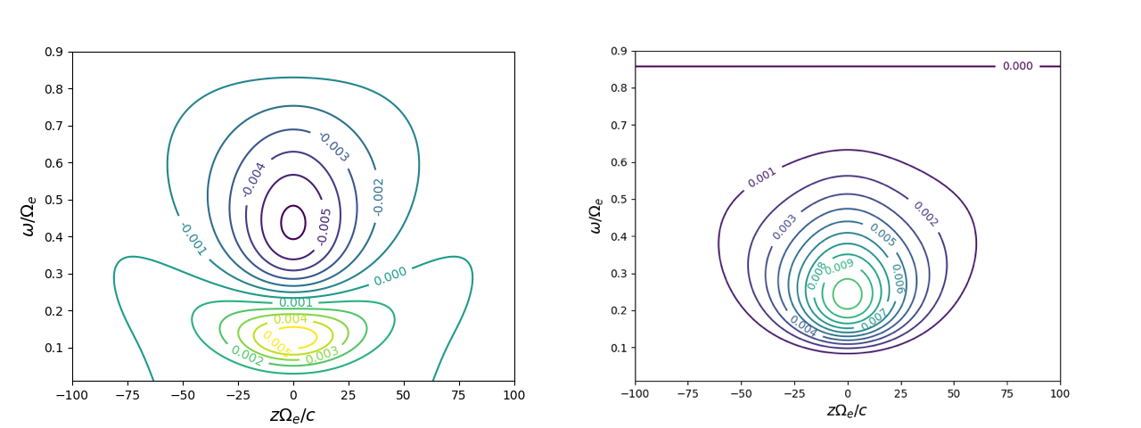
(a)                                                                 (b)

Figure 1: Contour plots of $W(z,t=0,\omega)/\Omega_{e}$ (a) and $\Gamma(z,t=0,\omega)/\Omega_{e}$ (b) are shown for normalized parameters $\omega_{p}/\Omega_{e}=5$, $n_{e}/n=6\times 10^{-3}$, $w_{\parallel e}=0.2c$, $w_{\perp e}=0.53c$, $\xi=8.62\times 10^{-5}\Omega_{e}^{2}/c^{2}$.

From Eqs. (16) and (20), it can be shown that both $W(z,t,\omega)$ and $\Gamma(z,t,\omega)$ scale as $\sim\zeta^{4}$, which accounts for most of the spatial non-uniformity of hot electron response, characterized by the length scale $(A\xi)^{-1/2}$ as clearly illustrated by Fig. 1 (cf. A). Thus, at the leading order, hot electrons can be considered as a non-uniform source neglecting magnetic field non-uniformity. Although not necessary, this assumption will help simplifying our analytical derivations in the remainder of this work, starting with Sec. 2.2 (cf. A for more details).

With the knowledge of $W(z,t,\omega)$ and $\Gamma(z,t,\omega)$, the nonlinear evolution of the chorus spectrum can be derived from the integration of Eqs. (11) and (14) along the characteristics, recalling that the right hand sides are, respectively, $2\Gamma(z,t,\omega)I(z,t,\omega)$ and $-W(z,t,\omega)$ as noted above. Thus, solutions are formally written as

$$I(z,t,\omega)=I_{\omega 0}\left(T_{\omega}^{-1}(T_{\omega}(z)-t)\right)\exp\left(2\int_{T_{\omega}^{-1}(T_{\omega}(z)-t)}^{z}\frac{dz^{\prime}}{v_{g\omega}(z^{\prime})}\Gamma(z^{\prime},t-T_{\omega}(z)+T_{\omega}(z^{\prime}),\omega)\right)\;,$$ (22)

for the wave packet intensity $I(z,t,\omega)$, where

$$T_{\omega}(z)\equiv\int_{0}^{z}\frac{dz^{\prime}}{v_{g\omega}(z^{\prime})}\;.$$ (23)

Meanwhile, a similar solution can be written for phase shift $\varphi(z,t,\omega)\equiv\varphi_{k}(z,t)|_{k=K(z,\omega)}$

$$\varphi(z,t,\omega)=\varphi_{\omega 0}\left(T_{\omega}^{-1}(T_{\omega}(z)-t)\right)-\int_{T_{\omega}^{-1}(T_{\omega}(z)-t)}^{z}\frac{dz^{\prime}}{v_{g\omega}(z^{\prime})}W(z^{\prime},t-T_{\omega}(z)+T_{\omega}(z^{\prime}),\omega)\;.$$ (24)

In the linear limit, where $W(z,t,\omega)=W(z,t=0,\omega)$ and $\Gamma(z,t,\omega)=\Gamma(z,t=0,\omega)$, Eqs. (22) and (24) are readily computed and corresponding solutions are shown in the contour plots of Fig. 2 for the same parameters of Fig. 1 and $z\Omega_{e}/c=50$.

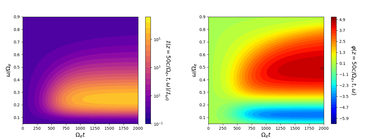
(a)                                                                 (b)

Figure 2: Contour plots of $I(z,t,\omega)/I_{\omega 0}$ (a) and $\varphi(z,t,\omega)$ (b) are shown for the linear evolution of the whistler wave packet and the same normalized parameters of Fig. 1. Here $I_{\omega 0}={\rm const}$ and $\varphi_{\omega 0}=0$ have been assumed together with $z\Omega_{e}/c=50$.

Nonlinear evolution is all embedded in the time dependence of $W(z,t,\omega)$ and $\Gamma(z,t,\omega)$. In particular, we will show below that chorus chirping may be understood as the spectral frequency peak of $I(z,t,\omega)$ at a given spatial position shifting in time. Meanwhile, since the growth of the spectral peak is due to spontaneous emission of whistler waves excited by hot electrons at the proper (instantaneous) wavelength and frequency, chorus nonlinear evolution is, thus, clearly associated with maximization of wave particle power transfer (Vomvoridis ., 1982; Trakhtengerts ., 2004; Omura ., 2008), as noted to be the case also for Alfvénic fluctuations in magnetized fusion plasmas (L. Chen  Zonca, 2016; Zonca, Chen, Briguglio, Fogaccia, Vlad  Wang, 2015). We will later come back to this very important point, with more insights and comments on the underlying physics. Summarizing, this analysis shows that chorus chirping rate can be predicted via analyzing $\partial_{t}\Gamma(z,t,\omega)$. In particular, $\partial_{t}\Gamma$ can be derived from $\partial_{t}f_{0}$, that is from manipulation of the Dyson-like equation, given in Sec. 2.2, as remarked in the Introduction. This derivation is carried out in Sec. 3, where we also show how $\partial_{t}\Gamma(z,t,\omega)$ and $\partial_{t}W(z,t,\omega)$ are interlinked (Zonca ., 2017).

2.2 Phase Space Dynamics

As shown in Sec. 2.1, hot electrons are localized about the equator and plasma non-uniformity effects are dominated by the $\sim\zeta^{4}$ scaling of both $W(z,t,\omega)$ and $\Gamma(z,t,\omega)$. Thus, as noted in A, hot electrons can be approximated as a non-uniform source, characterized by the length scale $(A\xi)^{-1/2}$, neglecting magnetic field non-uniformity. This assumption helps simplifying our analytical derivations below and, thus, we choose to adopt it in the following. In order to simplify presentation, we also assume $\omega^{2}/\omega_{p}^{2}\ll 1$, so that expressions of $W(z,t,\omega)$ and $\Gamma(z,t,\omega)$ are reduced to

$$W(z,t,\omega)+i\Gamma(z,t,\omega)=\frac{n_{e}}{n}\zeta^{4}\frac{\omega(\Omega_{e}-\omega)^{2}}{\Omega_{e}}\left\langle\frac{1}{\Omega_{e}+kv_{\parallel}-\omega}\left[\frac{kv_{\perp}^{2}}{2\omega}\frac{\partial}{\partial v_{\parallel}}-\frac{\Omega_{e}}{\omega}\right]\hat{f}_{0}\right\rangle\;,$$ (25)

Here and in the following, $k=K(z=0,\omega)$ will always be assumed as obtained from the solution of the linear dispersion relation, $D_{w}=0$. Meanwhile, as illustrated in A, we have integrated Eq. (20) by parts in $v_{\perp}$, extracted the expected hot electron non-uniformity scaling $\sim\zeta^{4}$, and denoted the response neglecting magnetic field non-uniformity as $f_{0}\equiv n_{e}\hat{f}_{0}$. Equation (25) suggests the connection of the phase shift and driving rate by a localized hot electron source with that by a uniform hot electron source in uniform magnetic field. To make this more explicit, let us introduce the rescaled phase shift and driving rate, $\bar{W}(z,t,\omega)$ and $\bar{\Gamma}(z,t,\omega)$, defined as

$$W(z,t,\omega)+i\Gamma(z,t,\omega)\equiv\zeta^{4}\frac{\omega(\Omega_{e}-\omega)^{2}}{\Omega_{e}^{2}}\left(1-\frac{v_{r\omega}}{v_{g\omega}}\right)^{-2}\left[\bar{W}(z,t,\omega)+i\bar{\Gamma}(z,t,\omega)\right]\;,$$ (26)

where $v_{r\omega}\equiv(\omega-\Omega_{e})/k$ is the resonant velocity, and $v_{g\omega}=v_{g\omega}(z=0)$ is the group velocity at the equator, defined below Eq. (16). Thus, we rewrite Eq. (25) as

$$\bar{W}(z,t,\omega)+i\bar{\Gamma}(z,t,\omega)=\frac{n_{e}}{n}\left(1-\frac{v_{r\omega}}{v_{g\omega}}\right)^{2}\left\langle\frac{\Omega_{e}}{\Omega_{e}+kv_{\parallel}-\omega}\left[\frac{kv_{\perp}^{2}}{2\omega}\frac{\partial}{\partial v_{\parallel}}-\frac{\Omega_{e}}{\omega}\right]\hat{f}_{0}\right\rangle\;.$$ (27)

The usefulness of introducing the factor $(1-v_{r\omega}/v_{g\omega})^{2}$, where both resonant and group velocity are computed at $z=0$, will be clarified in Sec. 3. There, we will also show that residual spatiotemporal dependences of $\hat{f}_{0}$, $\bar{W}$, and $\bar{\Gamma}$ will be via $t-z/v_{g\omega}$.

In the presence of a fluctuation spectrum in the form of Eq. (7), the hot electrons distribution function, $f\equiv n_{e}\hat{f}$ can be written as

$$\hat{f}(z,t)=\hat{f}_{0}(z,t)+\frac{1}{2}\sum_{k}\left(e^{iS_{k}(z,t)+i\alpha}\delta\hat{\bar{f}}_{k}(z,t)+c.c.\right)\;,$$ (28)

where $\hat{f}_{0}$, introduced in Eq. (25), denotes the $k=0$ component of $\hat{f}$; and, for brevity, we have omitted the velocity space dependences of hot electron response. Similar to Eq. (18), Equation (28) follows from the fact that, given the chorus wave packet polarization properties discussed in Sec. 2.1,

$$\frac{e}{m}\left(\delta\bar{\bm{E}}_{k}+\frac{\bm{v}\times\delta\bar{\bm{B}}_{k}}{c}\right)\cdot\frac{\partial}{\partial\bm{v}}=i\frac{e}{m}v_{\perp}\delta\bar{E}_{k}e^{i\alpha}\left[\frac{k}{\omega}\frac{\partial}{\partial v_{\parallel}}+\left(1-\frac{kv_{\parallel}}{\omega}\right)\left(\frac{1}{v_{\perp}}\frac{\partial}{\partial v_{\perp}}+\frac{i}{v_{\perp}^{2}}\frac{\partial}{\partial\alpha}\right)\right]\;.$$ (29)

The evolution equation for $\hat{f}_{0}$ can be obtained from the Vlasov equation

$$\left(\partial_{t}+v_{\parallel}\partial_{z}\right)\hat{f}_{0} = \frac{1}{4}\sum_{k}i\frac{e}{m}v_{\perp}\delta\bar{E}_{k}\left[\frac{k}{\omega}\frac{\partial}{\partial v_{\parallel}}+\left(1-\frac{kv_{\parallel}}{\omega}\right)\left(\frac{1}{v_{\perp}}\frac{\partial}{\partial v_{\perp}}+\frac{1}{v_{\perp}^{2}}\right)\right]\delta\hat{\bar{f}}_{k}^{*}$$ (30)

$$-\frac{1}{4}\sum_{k}i\frac{e}{m}v_{\perp}\delta\bar{E}_{k}^{*}\left[\frac{k}{\omega}\frac{\partial}{\partial v_{\parallel}}+\left(1-\frac{kv_{\parallel}}{\omega}\right)\left(\frac{1}{v_{\perp}}\frac{\partial}{\partial v_{\perp}}+\frac{1}{v_{\perp}^{2}}\right)\right]\delta\hat{\bar{f}}_{k}\;.$$

Meanwhile, the fluctuating component of the hot electron response is given by

$${\cal L}_{k}\delta\hat{\bar{f}}_{k} \equiv \left[kv_{\parallel}+\Omega_{e}-\omega-i\left(\partial_{t}+v_{\parallel}\partial_{z}\right)\right]\delta\hat{\bar{f}}_{k}$$ (31)

$$=\frac{e}{m}v_{\perp}\delta\bar{E}_{k}\left[\frac{k}{\omega}\frac{\partial}{\partial v_{\parallel}}+\left(1-\frac{kv_{\parallel}}{\omega}\right)\frac{1}{v_{\perp}}\frac{\partial}{\partial v_{\perp}}\right]\hat{f}_{0}\;.$$

Here, ${\cal L}_{k}$ is a first order partial differential operator that can be “formally inverted” as propagator ${\cal L}_{k}^{-1}$, which is an integral operator. Equation (31) applies both linearly and nonlinearly; i.e., when $\hat{f}_{0}$ is evolving in time due to resonant wave particle interactions. In particular, the action of the $\left(\partial_{t}+v_{\parallel}\partial_{z}\right)$ operator on the phase modulation due to $\delta\bar{E}_{k}=|\delta\bar{E}_{k}|e^{i\varphi_{k}}$ must be computed noting that the hot electron induced frequency ($\Delta_{\omega}$) and wave number ($\Delta_{k}$) shifts due to an incremental change in the fluctuation spectrum still satisfy the whistler wave dispersion relation with good approximation. This assumption is based on observations that chorus waves propagate in whistler mode; and it is consistent with the interpretation of chorus chirping as “whistler seeds” that are excited in sequence and amplified by wave particle resonant interactions with hot electrons originally proposed by (Omura  Nunn, 2011). Thus, $\omega$ and $k$ in Eqs. (30) and (31) denote the wave packet frequency and wave number in the presence of the hot electron source and the finite amplitude chorus. The effect of the nonlinear frequency and wave number shifts due to an incremental change in the fluctuation spectrum is discussed in Sec. 4. Meanwhile, $\omega$ and $k$ in Eqs. (30) and (31) are interpreted as elements of the whistler fluctuation spectrum that is considered dense (nearly continuous) and is self-consistently evolving in time as a whole in the presence of the hot electron free energy source (Zonca ., 2017; Tao ., 2020), rather than considered as properly chosen “whistler seeds” that are representative of the selected chorus element (Omura  Nunn, 2011). This is one of the main differences of the present work with respect to the earlier analysis by (Omura  Nunn, 2011), as discussed in the Introduction. The other one consists in the analytic solution for the self-consistent nonlinear hot electron response in phase space (Zonca ., 2017; Tao ., 2020), which is discussed below. Section 4 also allows us to reconcile different interpretations of chorus chirping (Omura  Nunn, 2011)) inside the same framework with a self-consistent comprehensive vision and to address some of the issues regarding sub-elements as presented in the recent work by Tsurutani . (2020).

When

$$\delta\hat{\bar{f}}_{k}={\cal L}_{k}^{-1}\left\{\frac{e}{m}v_{\perp}\delta\bar{E}_{k}\left[\frac{k}{\omega}\frac{\partial}{\partial v_{\parallel}}+\left(1-\frac{kv_{\parallel}}{\omega}\right)\frac{1}{v_{\perp}}\frac{\partial}{\partial v_{\perp}}\right]\hat{f}_{0}\right\}\;,$$ (32)

is substituted back into Eq. (30), the “formal solution” for $\hat{f}_{0}$ is obtained and can be cast in the form of a Dyson-like equation (Dyson, 1949; Schwinger, 1951; Itzykson  J.-B. Zuber, 1980)

$$\left(\partial_{t}+v_{\parallel}\partial_{z}\right)\hat{f}_{0} = \frac{1}{4}\sum_{k}i\frac{e}{m}v_{\perp}\delta\bar{E}_{k}\left[\frac{k}{\omega}\frac{\partial}{\partial v_{\parallel}}+\left(1-\frac{kv_{\parallel}}{\omega}\right)\left(\frac{1}{v_{\perp}}\frac{\partial}{\partial v_{\perp}}+\frac{1}{v_{\perp}^{2}}\right)\right]$$ (33)

$$\hskip 20.00003pt\times{\cal L}_{k}^{*-1}\left\{\frac{e}{m}v_{\perp}\delta\bar{E}_{k}^{*}\left[\frac{k}{\omega}\frac{\partial}{\partial v_{\parallel}}+\left(1-\frac{kv_{\parallel}}{\omega}\right)\frac{1}{v_{\perp}}\frac{\partial}{\partial v_{\perp}}\right]\hat{f}_{0}\right\}$$

$$-\frac{1}{4}\sum_{k}i\frac{e}{m}v_{\perp}\delta\bar{E}_{k}^{*}\left[\frac{k}{\omega}\frac{\partial}{\partial v_{\parallel}}+\left(1-\frac{kv_{\parallel}}{\omega}\right)\left(\frac{1}{v_{\perp}}\frac{\partial}{\partial v_{\perp}}+\frac{1}{v_{\perp}^{2}}\right)\right]$$

$$\hskip 20.00003pt\times{\cal L}_{k}^{-1}\left\{\frac{e}{m}v_{\perp}\delta\bar{E}_{k}\left[\frac{k}{\omega}\frac{\partial}{\partial v_{\parallel}}+\left(1-\frac{kv_{\parallel}}{\omega}\right)\frac{1}{v_{\perp}}\frac{\partial}{\partial v_{\perp}}\right]\hat{f}_{0}\right\}\;.$$

Connections of the present approach with the field theoretical description based on the Dyson-Schwinger equations are extensively analyzed in Refs. (L. Chen  Zonca, 2016; Zonca, Chen, Briguglio, Fogaccia, Vlad  Wang, 2015) as far as magnetized fusion plasma applications are concerned. Interested readers may find the same analyses specialized to chorus wave excitation in B. Here, we emphasize that the general theoretical framework (van Hove, 1954; Prigogine, 1962; Balescu, 1963; Al’Tshul’  Karpman, 1966; Dupree, 1966; Aamodt, 1967; Weinstock, 1969; Mima, 1973; Zonca, Chen, Briguglio, Fogaccia, Vlad  Wang, 2015; Zonca, Chen, Briguglio, Fogaccia, Milovanov ., 2015; L. Chen  Zonca, 2016; Zonca ., 2017) is of crucial importance for demonstrating that Eqs. (32) and (33) do indeed account for the phase space structures that determine the dominant nonlinear dynamics and phase space transport by chorus emission. In fact, the dynamic description given by Eq. (33) accounts for phase space nonlinear behaviors without fast temporal or spatial dependences, which correspond to the self-interaction of the fluctuation with the wavenumber of interest with itself. The resultant distortion of the hot electron distribution function, determined self-consistently in the presence of the finite amplitude fluctuation spectrum, constitutes the “renormalized” hot electron response of interest for the present application. Solving Eq. (33) together with the wave equations, Eqs. (11) and (14), preserves the crucial underlying physics of chorus nonlinear evolution but is beyond the scope of the present work. Here, we focus on chorus frequency chirping rather than on the details of phase space nonlinear dynamics and transport. Thus, in the next section we introduce a reduced (velocity space averaged) description of the Dyson-like equation that will allow us to derive nonlinear evolution equations for $\bar{W}(z,t,\omega)$ and $\bar{\Gamma}(z,t,\omega)$ and, thereby, analytically address the dynamics of chorus chirping.

3 Reduced Dyson-like equation

Let us reconsider the simplified expressions of $\bar{W}(z,t,\omega)$ and $\bar{\Gamma}(z,t,\omega)$, Eq. (27), obtained in Sec. 2.2. On the right hand side, formally consider $\hat{f}_{0}\equiv$
$\left(\partial_{t}+v_{\parallel}\partial_{z}\right)^{-1}\left(\partial_{t}+v_{\parallel}\partial_{z}\right)\hat{f}_{0}$ and use Eq. (33) for the expression of $\left(\partial_{t}+v_{\parallel}\partial_{z}\right)\hat{f}_{0}$. In other words, we formally manipulate the Dyson-like equation obtained in Sec. 2.2 and integrate in velocity space in order to obtain reduced expressions for time evolving $\bar{W}(z,t,\omega)$ and $\bar{\Gamma}(z,t,\omega)$ rather than solving Eq. (33) in the whole phase space (Zonca ., 2017; Tao ., 2020). This reduced approach becomes useful when the nonlinear particle response is dominated by resonant particles in the presence of a quasi-coherent (narrow) wave packet such as in the case of chorus. The same approach has been successfully applied to study energetic particle modes (Zonca, Chen, Briguglio, Fogaccia, Vlad  Wang, 2015) as well as the so called “fishbone” mode (L. Chen  Zonca, 2016) in fusion plasmas. Let us also recall the approximation introduced at the beginning of Sec. 2.2, by which we assume that hot electrons are a non-uniform source localized about the equator, while the remaining dynamics is well described neglecting magnetic field non-uniformity. Thus, Eq. (23) gives $T_{\omega}(z)\simeq z/v_{g\omega}$ and $T^{-1}_{\omega}(t)\simeq v_{g\omega}t$. Furthermore, at any position $z$ sufficiently outside the localized non-uniform hot electron source, $I(z,t,\omega)$ and $\varphi(z,t,\omega)$ are predominantly functions of $t-z/v_{g\omega}$, as can be verified from Eqs. (22) and (24) computing $\partial_{t}$ and $\partial_{z}$ of those expressions. Repeating the same argument, predominant dependence on $t-z/v_{g\omega}$ can be demonstrated for $\hat{f}_{0}$, $\bar{W}$ and $\bar{\Gamma}$. Residual $z$ dependences are neglected, since they account for magnetic field non-uniformity, which is omitted here for simplicity, and modulation effects of the chorus wave packet due to the finite extent of the source region. These effects are reported in detailed numerical investigations by (Wu ., 2020), illustrating the role of magnetic field non-uniformity in breaking the symmetry between rising and falling tone chorus. In a more recent work (Tao ., 2021), chorus nonlinear dynamics due to wave-particle interactions and magnetic field non-uniformity have been analyzed on the same footing within a newly developed phenomenological “TaRA model”, as anticipated in the Introduction. The present simplified theoretical description reduces the dimensionality of the problem and allows us to adopt useful simplifications; e.g., $(\partial_{t}+v_{\parallel}\partial_{z})\simeq(1-v_{r\omega}/v_{g\omega})\partial_{t}$ when dealing with resonant particles. Numerical studies of the complete Dyson-like Eq. (33) will be given elsewhere.

Based on these assumptions, on the right hand side of Eq. (33) we can write

$$i\left(\delta\bar{E}_{k}{\cal L}_{k}^{*-1}\delta\bar{E}_{k}^{*}-\delta\bar{E}_{k}^{*}{\cal L}_{k}^{-1}\delta\bar{E}_{k}\right)=i\left(\delta\bar{E}_{k}{\cal L}_{k}^{*-1}{\cal L}_{k}^{-1}{\cal L}_{k}\delta\bar{E}_{k}^{*}-\delta\bar{E}_{k}^{*}{\cal L}_{k}^{-1}{\cal L}_{k}^{*-1}{\cal L}_{k}^{*}\delta\bar{E}_{k}\right)\;.$$ (34)

Noting

$${\cal L}_{k}^{*-1}{\cal L}_{k}^{-1}\simeq{\cal L}_{k}^{-1}{\cal L}_{k}^{*-1}\simeq\left[{\cal L}_{k}{\cal L}_{k}^{*}\right]^{-1}=\left[(\Omega_{e}+kv_{\parallel}-\omega)^{2}+(1-v_{r\omega}/v_{g\omega})^{2}\partial_{t}^{2}\right]^{-1}\;,$$ (35)

where, again, the notation $[...]^{-1}$ always denotes the inverse of an operator within the square brackets, Eq. (34) can be cast as

$$i\left(\delta\bar{E}_{k}{\cal L}_{k}^{*-1}\delta\bar{E}_{k}^{*}-\delta\bar{E}_{k}^{*}{\cal L}_{k}^{-1}\delta\bar{E}_{k}\right) = i\left\{\delta\bar{E}_{k}\left[(\Omega_{e}+kv_{\parallel}-\omega)^{2}+(1-v_{r\omega}/v_{g\omega})^{2}\partial_{t}^{2}\right]^{-1}{\cal L}_{k}\delta\bar{E}_{k}^{*}\right.$$ (36)

$$\left.-\delta\bar{E}_{k}^{*}\left[(\Omega_{e}+kv_{\parallel}-\omega)^{2}+(1-v_{r\omega}/v_{g\omega})^{2}\partial_{t}^{2}\right]^{-1}{\cal L}_{k}^{*}\delta\bar{E}_{k}\right\}$$

$$\simeq 2|\delta\bar{E}_{k}|\left[(\Omega_{e}+kv_{\parallel}-\omega)^{2}+(1-v_{r\omega}/v_{g\omega})^{2}\partial_{t}^{2}\right]^{-1}$$

$$\times(1-v_{r\omega}/v_{g\omega})\partial_{t}|\delta\bar{E}_{k}|\;.$$

Here, as it can be verified by inspection, the operators action on the phase dependences in $\delta\bar{E}_{k}=|\delta\bar{E}_{k}|e^{i\varphi_{k}}$ and its complex conjugate cancel each other and only $(1-v_{r\omega}/v_{g\omega})\partial_{t}|\delta\bar{E}_{k}|$ survives. Using this expression and substituting Eq. (33) back into Eq. (27), we finally obtain, after tedious but straightforward algebra (cf. Appendix C.1)

$$\bar{W}(\bar{\omega})+i\bar{\Gamma}(\bar{\omega}) = \frac{n_{e}}{n}\left(1-\frac{v_{r\bar{\omega}}}{v_{g\bar{\omega}}}\right)^{2}\left\langle\frac{v_{\perp}^{4}}{2}\Omega_{e}\left[\Omega_{e}+\bar{k}v_{\parallel}-\bar{\omega}-i(1-v_{r\bar{\omega}}/v_{g\bar{\omega}})\partial_{t}\right]^{-1}\right.$$ (37)

$$\times\left(\frac{\bar{k}}{\bar{\omega}}\frac{\partial}{\partial v_{\parallel}}-\frac{2}{\left\langle v_{\perp}^{2}\right\rangle}\frac{\Omega_{e}}{\bar{\omega}}\right)\left(\partial_{t}+v_{\parallel}\partial_{z}\right)^{-1}\sum_{k}\frac{e^{2}}{2m^{2}}|\delta\bar{E}_{k}|\frac{k}{\omega}\frac{\partial}{\partial v_{\parallel}}$$

$$\times\left[(\Omega_{e}+kv_{\parallel}-\omega)^{2}+(1-v_{r\omega}/v_{g\omega})^{2}\partial_{t}^{2}\right]^{-1}(1-v_{r\omega}/v_{g\omega})$$

$$\times\left.\partial_{t}|\delta\bar{E}_{k}|\left(\frac{k}{\omega}\frac{\partial}{\partial v_{\parallel}}-\frac{2}{\left\langle v_{\perp}^{2}\right\rangle}\frac{\Omega_{e}}{\omega}\right)\hat{f}_{0}\right\rangle\;.$$

Here, we have repeatedly integrated by parts in $v_{\perp}$, from outside to the inside, in order to remove any $\partial/\partial v_{\perp}$ in the final expression. Moreover, for simplicity of notation, we have explicitly indicated only the frequency dependence of $\bar{W}$ and $\bar{\Gamma}$, leaving implicit the dependence on $t-z/v_{g\bar{\omega}}$. Finally $\left\langle v_{\perp}^{2}\right\rangle\equiv\left\langle v_{\perp}^{2}\hat{f}_{0}\right\rangle/\left\langle\hat{f}_{0}\right\rangle$, and we have denoted the current frequency and wave number satisfying the lowest order whistler wave dispersion relation as $\bar{\omega}$ and $\bar{k}$ in order to distinguish them from $\omega$ and $k$ in the running summation over the fluctuation spectrum.

Equation (37) still contains all the information embedded in the solution of the Dyson-like equation, Eq. (33), via complicated integro-differential operators. In order to make further progress, we explicitly carry out the velocity space integration adopting two assumptions: (i) the chorus spectrum is narrow, such that $(\omega,k)\simeq(\bar{\omega},\bar{k})$ and $\partial_{t}|\delta\bar{E}_{k}|\simeq\partial_{t}|\delta\bar{E}_{\bar{k}}|$; (ii) chorus chirping is due to the subsequent emission of different waves belonging to the whistler wave continuum, which are excited in turns to maximize wave particle power transfer. The assumption (ii) was already introduced in the remarks following Eq. (33) in Sec. 2.2 and will be further discussed below in Sec. 4. Meanwhile, both assumptions are based on the chorus spectral features and are the same as those of fluctuation spectra in the aforementioned fusion applications (L. Chen  Zonca, 2016; Zonca, Chen, Briguglio, Fogaccia, Vlad  Wang, 2015). After tedious but straightforward algebra, some details of which are reported in Appendix C.2 for interested readers, real and imaginary parts of Eq. (37) can be cast as

$$\Omega_{e}^{-1}\partial_{t}\bar{W}(\bar{\omega}) = \left[\Omega_{e}\frac{\partial}{\partial\bar{\omega}}-\frac{2\Omega_{e}^{2}}{\bar{k}^{2}\left\langle v_{\perp}^{2}\right\rangle}\left(1-\frac{v_{r\bar{\omega}}}{v_{g\bar{\omega}}}\right)\right]\Omega_{e}\frac{\partial}{\partial\bar{\omega}}$$ (38)

$$\times\sum_{k}\frac{\left(\omega-\bar{\omega}\right)}{2\Omega_{e}}\left[\frac{\left(\omega-\bar{\omega}\right)^{2}}{4\Omega_{e}^{2}}+\Omega_{e}^{-2}\partial_{t}^{2}\right]^{-1}$$

$$\times\frac{\left\langle\left\langle\omega_{{\rm tr}k}^{4}\right\rangle\right\rangle}{4\Omega_{e}^{4}(1-v_{r\omega}/v_{g\omega})^{4}}\left(\frac{\bar{\Gamma}(\omega)+\bar{\Gamma}(\bar{\omega})}{2}\right)\;;$$

and, denoting as $\bar{\Gamma}_{L}$ the linear (initial) normalized hot electron driving rate,

$$\bar{\Gamma}(\bar{\omega})-\bar{\Gamma}_{L}(\bar{\omega}) = \left[\Omega_{e}\frac{\partial}{\partial\bar{\omega}}-\frac{2\Omega_{e}^{2}}{\bar{k}^{2}\left\langle v_{\perp}^{2}\right\rangle}\left(1-\frac{v_{r\bar{\omega}}}{v_{g\bar{\omega}}}\right)\right]\Omega_{e}\frac{\partial}{\partial\bar{\omega}}$$ (39)

$$\times\sum_{k}\left[\frac{\left(\omega-\bar{\omega}\right)^{2}}{4\Omega_{e}^{2}}+\Omega_{e}^{-2}\partial_{t}^{2}\right]^{-1}$$

$$\times\frac{\left\langle\left\langle\omega_{{\rm tr}k}^{4}\right\rangle\right\rangle}{4\Omega_{e}^{4}(1-v_{r\omega}/v_{g\omega})^{4}}\left(\frac{\bar{\Gamma}(\omega)+\bar{\Gamma}(\bar{\omega})}{2}\right)\;,$$

where we have introduced the wave particle trapping frequency definition

$$\left\langle\left\langle\omega_{{\rm tr}k}^{4}\right\rangle\right\rangle\equiv\left\langle v_{\perp}^{2}\omega_{{\rm tr}k}^{4}\hat{f}_{0}\right\rangle/\left\langle v_{\perp}^{2}\hat{f}_{0}\right\rangle\;,$$ (40)

with $\omega_{{\rm tr}k}^{2}=|(e/m)k^{2}v_{\perp}\delta\bar{E}_{k}/\omega|$.

Equations (38) and (39) are still complicated nonlinear integro-differential equations, but they have been significantly simplified (or reduced) with respect to the original Dyson-like equation, Eq. (33). These equations are the primary theoretical results of the present work and show that $\bar{W}$ and $\bar{\Gamma}$ evolution equations are interlinked, as expected and as anticipated in Sec. 2.1. They describe a variety of nonlinear dynamics, including chorus chirping and modulation of the chorus wave packets on a time scale $\sim\left\langle\left\langle\omega_{{\rm tr}k}^{4}\right\rangle\right\rangle^{-1/4}$. To see this more clearly, let us introduce the optimal ordering for Eqs. (38) and (39). The width of the fluctuation spectrum can be estimated as

$$\frac{\left|\omega-\bar{\omega}\right|}{2\Omega_{e}}\sim\frac{\partial_{t}\bar{W}}{\Omega\bar{\Gamma}_{NL}}\;.$$ (41)

Meanwhile, assuming $|\partial_{\bar{\omega}}^{2}\Gamma_{NL}|\raisebox{-3.01385pt}{$\stackrel{{\scriptstyle\textstyle>}}{{\sim}}$}\ |\partial_{\bar{\omega}}^{2}\Gamma_{L}|$, ordering all terms of Eq. (39) on the same footing gives

$$|\partial_{t}|\sim\left|\omega-\bar{\omega}\right|\sim|\partial_{\bar{\omega}}|^{-1}\sim\left\langle\left\langle\omega_{{\rm tr}k}^{4}\right\rangle\right\rangle^{1/4}\sim\hat{\gamma}_{e}\;,$$ (42)

where $\hat{\gamma}_{e}$ is the peak value of the linear hot electron driving rate at the equator. Equation (42) describes a whistler wave packet that grows and saturates locally due to wave particle trapping. However, if chirping consistent with Eq. (1) sets in as in chorus spontaneous emission, saturation at the level of Eq. (42) is not possible and the wave packet can grow further. Equation (39), then, suggests

$$|\partial_{t}|\sim\left\langle\left\langle\omega_{{\rm tr}k}^{4}\right\rangle\right\rangle^{1/2}|\partial_{\bar{\omega}}|\sim\frac{\left\langle\left\langle\omega_{{\rm tr}k}^{4}\right\rangle\right\rangle^{1/2}}{\left|\omega-\bar{\omega}\right|}\raisebox{-3.01385pt}{$\stackrel{{\scriptstyle\textstyle>}}{{\sim}}$}\ \left|\omega-\bar{\omega}\right|\;.$$ (43)

This ordering corresponds to a characteristic nonlinear time, $\tau_{NL}\sim|\partial_{t}|^{-1}\sim\Gamma_{NL}^{-1}$ that is shorter than the wave particle auto-correlation time, $|\Delta\omega|^{-1}\sim\left|\omega-\bar{\omega}\right|^{-1}$. In particular, this ordering is consistent with chorus chirping, and Eq. (39) readily yields Eq. (1) when we assume a quasi-coherent (nearly monochromatic) fluctuation spectrum. In fact, keeping the leading terms only in Eq. (39), consistent with Eq. (43), we have that $\Omega_{e}^{-2}\partial_{t}^{2}$ dominates in the integral operator definition, Eq. (39), and

$$\frac{\partial^{2}}{\partial t^{2}}\bar{\Gamma}_{NL}(\bar{\omega})\simeq\left(\sum_{k}\frac{\left\langle\left\langle\omega_{{\rm tr}k}^{4}\right\rangle\right\rangle}{4(1-v_{r\omega}/v_{g\omega})^{4}}\right)\frac{\partial^{2}}{\partial\bar{\omega}^{2}}\bar{\Gamma}_{NL}(\bar{\omega}).$$ (44)

This result suggest that there exists a self similar solution for $\bar{\Gamma}_{NL}$ that ballistically propagates in $\omega$-space at a rate given by the square root of the quantity in square parentheses on the right hand side. This ballistic propagation corresponds to the analogous ballistic propagation of hot electron phase space structures, described by Eq. (33); and it is in one-on-one correspondence with the analogous ballistic propagation of phase space zonal structures connected with energetic particle avalanches in fusion plasmas (L. Chen  Zonca, 2016; Zonca, Chen, Briguglio, Fogaccia, Vlad  Wang, 2015). Details obviously depend on the actual form of the spectrum, but it is readily verified that, for nearly monochromatic chorus element, Eq. (44) yields

$$\frac{\partial\omega}{\partial t}=\pm\frac{1}{2}\frac{\left\langle\left\langle\omega_{{\rm tr}k}^{4}\right\rangle\right\rangle^{1/2}}{(1-v_{r\omega}/v_{g\omega})^{2}}\;.$$ (45)

Thus, the present theoretical framework is consistent with both upward and downward frequency sweeping of chorus structures and, thus, consistent with the recent work by Wu . (2020). This is the first theoretical prediction for the downward chirping of parallel propagating waves, as far as we are aware of. However, it should also be noted that statistical observations of chorus falling tones show that they are mainly very oblique rather than parallel (Li ., 2011), and that Mourenas . (2015) have predicted the possible existence of both positive and negative frequency chirping for such very oblique chorus waves based on the maximization of the nonlinear growth rate of Shklyar  Matsumoto (2011). More detailed discussions on the chirping direction will be given below in Sec. 4. Focusing, here, on the positive sign of Eq. (45), by direct inspection it can be noted that it coincides with Eq. (1) for $R=1/2$ as anticipated in the Introduction (Vomvoridis ., 1982). Equation (45) improves an earlier estimate by the same authors (Zonca ., 2017) and, to our knowledge, is the first self-consistent analytical demonstration of the conjecture by Vomvoridis . (1982) in its exact initial formulation. More generally, Eq. (44) suggests why the chorus chirping rate is not always given by $R=1/2$, the limiting case for a nearly monochromatic spectrum, but may vary depending on the excitation conditions; e.g., the initial hot electron distribution function.

4 On chorus chirping

In order to further illuminate the features of chorus dynamics as predicted by Eqs. (38) and (39) , we have solved them numerically, together with the wave equations of Sec. 2.1, using a 4th order Runge-Kutta method. To exploit the dense nature of the whistler wave spectrum, we introduce the dimensionless intensity ${\cal I}(\omega)$ such that nonlinearity effects become important when ${\cal I}(\omega)\sim{\cal O}(1)$ (cf. D).

Assuming fixed $z\Omega_{e}/c=50$ and parameters as in Fig. 1, the nonlinear evolution of ${\cal I}(z=50c/\Omega_{e},t,\omega)$ is shown in Fig. 3. Here, rather than assuming a specific form of the initial spectrum, we assumed vanishing initial conditions and a constant slow external stirring that, in the absence of supra-thermal electrons, would give an intensity spectrum ${\cal I}={\cal S}^{2}\Omega_{e}^{2}t^{2}$, corresponding to $|\delta\bar{E}_{k}|$ linearly increasing with time (cf. D). In Fig. 3, the source strength is ${\cal S}=2\times 10^{-5}$. Furthermore, we use a discretization in $\omega$ space with $221$ grid points in the interval $\omega/\Omega_{e}\in[0.05,0.9]$ and adopt a Savitzky–Golay filter fitting sub-sets of 19 adjacent data points with a fourth order degree polynomial to ensure regularity of the derivatives in $\omega$-space. A fourth order Runge-Kutta integration in time is adopted with variable time step, gradually decreasing from an initial $\Omega_{e}\Delta t=1.25\times 10^{-1}$ in the early linear evolution to $\Omega_{e}\Delta t=3.125\times 10^{-2}$ in the later nonlinear phase at $\Omega_{e}t>1750$. This choice ensures that Courant condition is well satisfied. The routine solving Eqs. (60) to (64), closed by Eqs. (65) and (66) together with the aforementioned boundary conditions, is written in Python and uses Python standard libraries. In order to illustrate the robustness of the present numerical results as parameters are varied, Fig. 4 shows the nonlinear evolution of ${\cal I}(z=50c/\Omega_{e},t,\omega)$ for ${\cal S}=\sqrt{2}\times 10^{-5}$ and same physical parameters of Fig. 3. In this case, the Savitzky–Golay filter is reduced to fitting sub-sets of 15 adjacent data points with a fourth order degree polynomial.

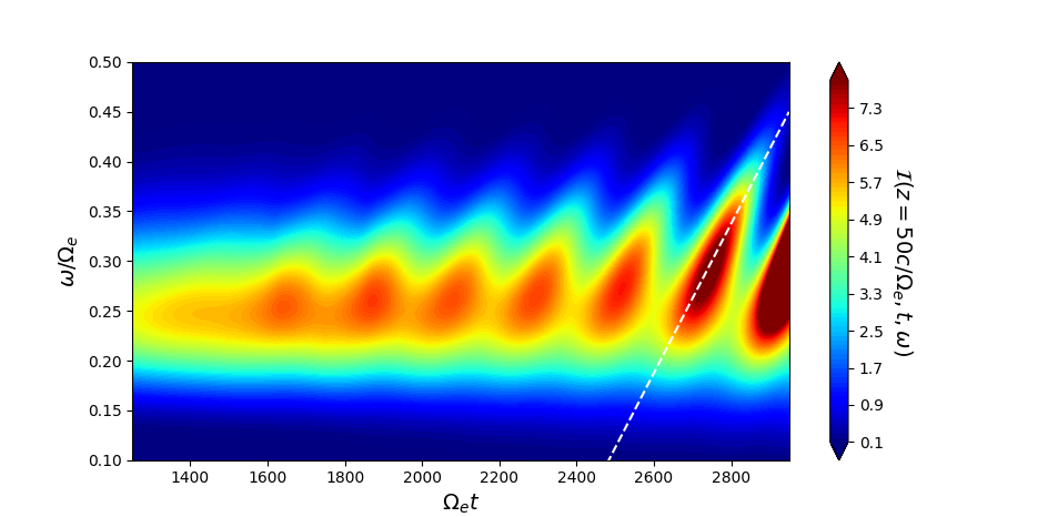
Figure 3: Contour plot of the nonlinear evolution of ${\cal I}(\omega)$ for a uniform source ${\cal S}=2\times 10^{-5}$ in Eq. (63). The position is fixed at $z\Omega_{e}/c=50$ and parameters are the same as in Fig. 1. The white dashed line passing through the chorus element beginning at $\Omega_{e}t\sim 2600$ represents the average chirping rate $\partial_{t}\omega_{0}=7.5\times 10^{-4}\Omega_{e}^{2}$.

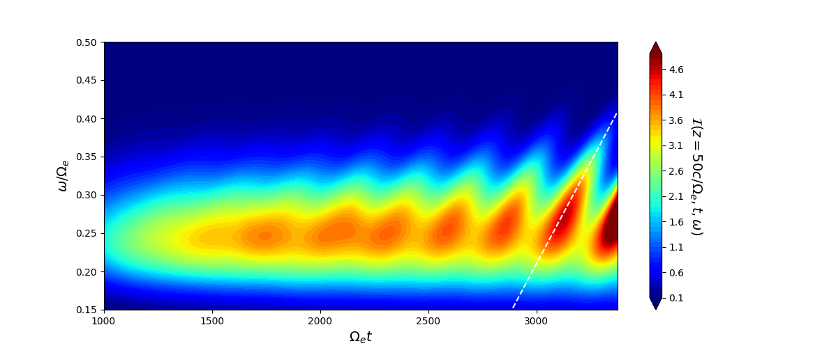
Figure 4: Contour plot of the nonlinear evolution of ${\cal I}(\omega)$ for a uniform source ${\cal S}=\sqrt{2}\times 10^{-5}$ in Eq. (63). As in Fig. 3, the position is fixed at $z\Omega_{e}/c=50$ and parameters are the same as in Fig. 1. The white dashed line passing through the chorus element beginning at $\Omega_{e}t\sim 3000$ represents the average chirping rate $\partial_{t}\omega_{0}=5.3\times 10^{-4}\Omega_{e}^{2}$ as obtained from PIC simulation by the DAWN code in (Tao ., 20171).

Various distinctive features clearly emerge in Fig. 3 and Fig. 4. After the initial formation of the “linear” fluctuation spectrum, clear modulations at the $\left\langle\left\langle\omega_{\rm{tr}k}^{4}\right\rangle\right\rangle^{1/4}$ frequency become increasingly more evident as the fluctuation intensity $\cal I$ grows larger than unity, as expected from the previous theoretical analysis and from (Tao ., 20171). Note that these modulations are different from the amplitude modulations within one chorus element leading to the so-called “subpackets” or “subelements” (Santolík ., 2003). However, they stem from the same physics; that is, the spectrum intensity modulation due to the finite frequency width of the wave packet as shown in Eqs. (60). Nonlinear oscillations, as intensity increases, are accompanied by gradually increasing frequency chirping, which can be both up or down. This behavior is consistent with Eq. (45) and, despite no clear falling tone chorus element is observed here, it is also consistent with the recent numerical investigation by (Wu ., 2020). Further strengthening of the nonlinear oscillations due to the continuous energy injection in the system by the uniform source ${\cal S}$, which is amplified via resonant wave particle power exchange and structure formation in the phase space, breaks the up-down symmetry in the chirping process because of the lack of symmetry (in frequency) of the linear drive about its maximum (cf. Fig. 1) and because of the symmetry breaking term in the first line on the right hand side of Eq. (61). Another origin of symmetry breaking in frequency chirping is due to the non-uniformity due to the ambient magnetic field (Wu ., 2020), which, however, is neglected for the sake of simplicity in the present theoretical analysis. Focusing on the rising tone chorus element beginning at $\Omega_{e}t\sim 2600$ in Fig. 3, the frequency chirping is well represented by Eq. (45) and is fitted by the average chirping rate $\partial_{t}\omega_{0}=7.5\times 10^{-4}\Omega_{e}^{2}$. For the somewhat weaker power injection in Fig. 4, the chirping of rising tone chorus element beginning at $\Omega_{e}t\sim 3000$ agrees remarkably well with the average chirping rate $\partial_{t}\omega_{0}=5.3\times 10^{-4}\Omega_{e}^{2}$ as obtained from PIC simulation by the DAWN code in (Tao ., 20171) and, again, is visually given by the white dashed line. The average chirping rate dependence on the fluctuation intensity further confirms Eq. (45). The average chirping rate is also confirmed by the instantaneous chirping rate of the intensity peak given in Fig. 5. Noting $\partial_{t}\omega_{0}/\Omega_{e}^{2}$ is starting from negative values, as noted above, is consistent with the possibility of both up- and down-chirping and, thus, with Eq. (45). However, here, we cannot observe a clear formation of a falling tone chorus element unlike in (Wu ., 2020), despite the evidence of initial down-chirping. As the rising tone chorus element is clearly formed with the corresponding phase space structure, the chirping rate reaches up to its average value as visually suggested by the white dashed line in Fig. 3.

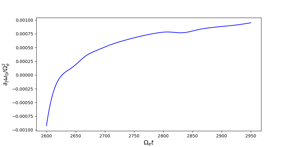
Figure 5: Instantaneous chirping rate of the intensity peak of the rising tone chorus element beginning at $\Omega_{e}t\sim 2600$ in Fig. 3.

Time evolution of intensity peak ${\cal I}_{0}(z=50c/\Omega_{e},t)$ and corresponding phase shift $\Delta\varphi_{0}(z=50c/\Omega_{e},t)$ for this chorus element are given in Fig. 6 and further clarify the underlying physics. An important conclusion we may draw from Fig. 6 is that intensity grows while $\Delta\varphi_{0}\simeq 0$; i.e., during phase locking. This behavior is due to phase bunching of both trapped and untrapped resonant particles, which most effectively drive the chorus wave-packet. The same behavior allows us drawing strong connection with the analogous behavior of energetic particle avalanches in fusion plasmas (Zonca, Chen, Briguglio, Fogaccia, Vlad  Wang, 2015; L. Chen  Zonca, 2016). Meanwhile, the intensity peak takes place when $\Delta\varphi_{0}=\pi$ and resonant particles phase locking is lost yielding the end of the chorus event. This mechanism can be viewed as the chorus wave packet slipping over the population of resonant electrons maximizing wave particle power extraction, and suggests the analogy with super-radiance in free electron lasers introduced by (Zonca, Chen, Briguglio, Fogaccia, Vlad  Wang, 2015; L. Chen  Zonca, 2016) with regard to energetic particle mode convective amplification in fusion plasmas. Analogies with the free electron laser were also noted by numerical simulation studies in (Soto-Chavez ., 2012).

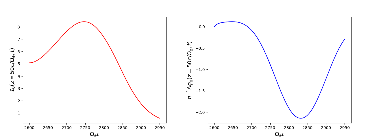
(a)                                                              (b)

Figure 6: Time evolution of intensity peak ${\cal I}_{0}(z=50c/\Omega_{e},t)$ (a) and corresponding phase shift $\Delta\varphi_{0}(z=50c/\Omega_{e},t)$ (b) for the rising tone chorus element beginning at $\Omega_{e}t\sim 2600$ in Fig. 3.

That it is indeed maximization of wave particle power transfer (Vomvoridis ., 1982; Omura ., 2008; Zonca, Chen, Briguglio, Fogaccia, Vlad  Wang, 2015; Zonca, Chen, Briguglio, Fogaccia, Milovanov ., 2015; L. Chen  Zonca, 2016) that dictates the nonlinear chorus dynamics and frequency chirping is further demonstrated by Fig. 7. Figure 7 (a) shows that the nonlinear frequency shift, $\Delta_{\omega}(z=50c/\Omega_{e},t)$, remains small during the whole nonlinear evolution and, in particular, much smaller than the dynamic range of frequency chirping, consistent with the assumption that each elementary wave constituting the chorus wave packet satisfies the whistler wave dispersion relation at the lowest order. Figure 7 (b), meanwhile, shows a snapshot of $\Delta_{\omega}(z=50c/\Omega_{e},t=2875/\Omega_{e})$. By definition, at the intensity peak the wave particle power transfer is maximized; and, since the chirping process is spontaneously triggered by the underlying instability, the nonlinear evolution follows the maximum possible intensity growth or minimum possible intensity decrease. In fact, it is important to recognize that power transfer is maximized even in the intensity decreasing phase (Zonca, Chen, Briguglio, Fogaccia, Vlad  Wang, 2015; Zonca, Chen, Briguglio, Fogaccia, Milovanov ., 2015; L. Chen  Zonca, 2016) .

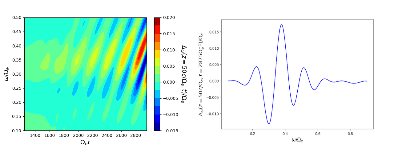
(a)                                                              (b)

Figure 7: Contour plot of the nonlinear frequency shift, $\Delta_{\omega}(z=50c/\Omega_{e},t)$ (a); and snapshot of $\Delta_{\omega}(z=50c/\Omega_{e},t=2875/\Omega_{e})$ (a).

Another aspect that is clarified by the present approach and is the issue of “subpackets” or “subelements” (Santolík ., 2003) formation within a single chorus element. While Fig. 3 and Fig. 4 display the spectrum intensity only, Fig. 8 illustrates the temporal structure of the perpendicular magnetic field fluctuation, $|\delta\bm{B}_{\perp}|/B_{e}$, reconstructed from Eqs. (7) and (9), for the rising tone chorus element beginning at $\Omega_{e}t\sim 2600$ in Fig. 3. The formation of subelements is clear, qualitatively and quantitatively consistent with the PIC simulation by the DAWN code done with the same parameters in (Tao ., 20171). This evidence supports the corresponding original interpretation provided therein that chorus sub-element formation is to be attributed to the phase modulation and “self-consistent evolution of resonant particle phase-space structures and spatiotemporal features of the fluctuation spectrum”, proposed by (O’Neil, 1965) when analyzing collisionless damping of nonlinear plasma oscillations. These results also clarify that nonlinear oscillations are connected with the width of the fluctuation intensity spectrum and stem from the same underlying physics, as noted above. In close connection and consistent with the present analysis, it is important to quote the recent statistical results from Zhang . (2020) on observed typical wave packet lengths, amplitudes, and frequency variations of rising tone chorus elements. Short packets have been explained by Zhang . (2020) and Nunn . (2021) as resulting from trapping-related amplitude modulations for packets longer than about 10 wave periods, and as a result of wave superposition of two well-separated waves sensibly farther than a trapping period for shorter packets. Formation of subpackets in chorus emission was also recently analyzed by (Hanzelka ., 2020) adopting the sequential triggering model by Omura  Nunn (2011).

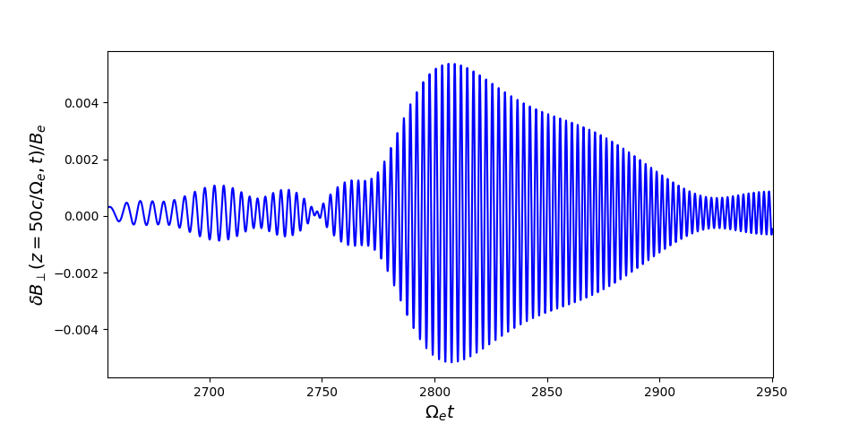
Figure 8: Temporal structure of the perpendicular magnetic field fluctuation, $|\delta\bm{B}_{\perp}|/B_{e}$ for the rising tone chorus element beginning at $\Omega_{e}t\sim 2600$ in Fig. 3. Formation of “subpackets” or “subelements” (Santolík ., 2003) is clearly illustrated.

Given the present theoretical analysis and numerical solutions, the explanation of chorus frequency chirping given by (Omura  Nunn, 2011) may seemingly be in contrast with the present results. As anticipated in the Introduction, the reason for frequency chirping was explained as due to the nonlinear current parallel to the wave magnetic field ($J_{B}$), which causes a nonlinear frequency shift. More precisely, the physics mechanism underlying chirping is the sequence of “whistler seeds” that are excited and amplified by wave particle resonant interactions with supra-thermal electrons. In the present work, the fluctuation spectrum is self-consistently evolved out of a very weak “white spectrum” source. Each oscillator in the wave spectrum can be characterized by a small nonlinear frequency shift (cf. Fig. 7). However, the wave packet that spontaneously evolves from the superposition of these oscillators sweeps upward in frequency to maximize wave particle power exchange. While doing so, self-consistency between chirping and rate of change of nonlinear frequency shift should be “locked”. This is visible in Fig. 9 (a), where the intensity peak frequency (blue line) of the chorus element considered in Fig. 3 is compared with the frequency of the corresponding peak of the rate of change of nonlinear frequency shift (red line). Recalling the discussion preceding Eq. (65), the rate of change of the resonant frequency is $\partial_{t}\omega_{\rm res}=(1-v_{r\omega}/v_{g\omega})\partial_{t}\Delta_{\omega}$. A snapshot at $\Omega_{e}t=2875$ of the fluctuation intensity and of the $\partial_{t}\omega_{\rm res}$ as a function of frequency is given in Fig. 9 (b).

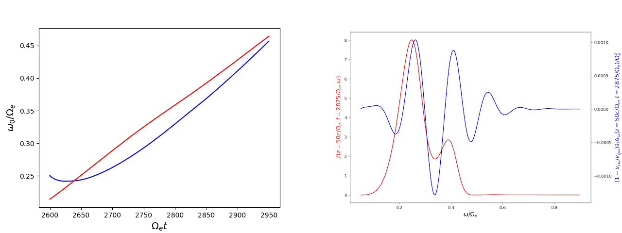
(a)                                                              (b)

Figure 9: (a) Time evolution of intensity peak frequency (blue line) and of the frequency of the peak of the corresponding maximum in the rate of change of nonlinear frequency shift (red line) for the rising tone chorus element beginning considered in Fig. 3. (b) Snapshot at $\Omega_{e}t=2875$ of the fluctuation intensity and of the $\partial_{t}\omega_{\rm res}$ as a function of frequency.

Thus, interpreting the “whistler seeds” of (Omura  Nunn, 2011) as the swinging oscillators in the wave packet at the intensity peak, one should obtain the frequency increase due to the chorus chirping as

$$\Delta\omega=\int(1-v_{r\omega_{0}(t^{\prime})}/v_{g\omega_{0}(t^{\prime})})\partial_{t^{\prime}}\Delta_{\omega_{0}(t^{\prime})}dt^{\prime}\;,$$

where integration is to be intended along the red line of Fig. 9 (a). The hence obtained frequency increase is $\Delta\omega/\Omega_{e}=0.24$ over the considered time interval, against the corresponding frequency shift, $\Delta\omega/\Omega_{e}=0.21$ of the intensity peak. Such a good agreement confirms the present explanation that reconciles the original interpretation of frequency chirping given by (Omura  Nunn, 2011) with the present theoretical analysis.

Further to this, and for the sake of completeness, we would like to recall the previous discussion about the formation of sub-packets in connection with Fig. 8. Recent statistics of 6 years of Van Allen Probes observations provided by Zhang . (2020) have shown that the frequency variation inside sufficiently long chorus wave packets is generally finite, in agreement with Refs. (Vomvoridis ., 1982; Omura ., 2008) and the present the expression, Eq. (45). However, faster frequency variations were found inside very short packets of duration less than 30 wave periods. Zhang . (2020) explained them as due to trapping effects for relatively high amplitudes, or as due to wave superposition for very short packets of moderate amplitudes and duration less than 10 wave periods. Such statistical results have been qualitatively reproduced by numerical simulations (Nunn ., 2021); and other previous works have also found some significant wave superposition during observations and simulations of chorus rising tones (Li ., 2011; Katoh  Omura, 2016; Crabtree ., 2017).

As a final remark, we would like to emphasize that the present theoretical analysis can also address some elements of the recent work by (Tsurutani ., 2020), based on observations using Van Allen Probe data and emphasizing that each chorus element is made of discrete sub-elements with constant frequency. Figure 7, in fact, supports that each nonlinear oscillator has a nonlinear frequency shift in the order of a few percent, consistent with observations by (Tsurutani ., 2020). The discrete steps, which are the essential elements of the rising tone chorus element, are instead beyond the description of the present theoretical study since, by definition in Eq. (59), we assume the continuous limit to analytically derive the present reduced model for chorus nonlinear dynamics. Within the same theoretical framework, it would be possible to solve the same equations in discretized form addressing, thus, the situation described by (Tsurutani ., 2020). This, however, is beyond the scope intended for the present work and hopefully will be addressed in the future.

5 Summary

In this work, we have presented a novel and comprehensive theoretical framework of chorus wave excitation, based on field theoretical methods introduced in (Zonca ., 2017) and in earlier works (Zonca, Chen, Briguglio, Fogaccia, Vlad  Wang, 2015; Zonca, Chen, Briguglio, Fogaccia, Milovanov ., 2015; L. Chen  Zonca, 2016). This theoretical framework allows us to self-consistently evaluate the renormalized phase space response of supra-thermal electrons, that is, the response accounting for self-interactions in the presence of finite amplitude whistler waves.

We have, furthermore, shown that the renormalized distribution function obeys a Dyson-like equation. Since our present aim is to investigate excitation and chirping of chorus waves, we further simplify the Dyson-like equation by taking its velocity space moments and, ultimately, obtain equations for the nonlinear growth rate and frequency shifts of whistler wave packets excited by an anisotropic (bi-Maxwellian) hot electron distribution function. Based on the structure of the hence derived governing equations, we analytically demonstrate for the first time that the chorus chirping rate is given by Eq. (1), originally proposed by (Vomvoridis ., 1982). As argued by (Vomvoridis ., 1982; Omura ., 2008), chorus chirping is due to maximization of wave particle power transfer, similar to analogous chirping observed in fusion plasmas (Zonca, Chen, Briguglio, Fogaccia, Vlad  Wang, 2015; Zonca, Chen, Briguglio, Fogaccia, Milovanov ., 2015; L. Chen  Zonca, 2016). In the light of present results, chorus chirping can be diagrammatically illustrated as in Fig. 10.

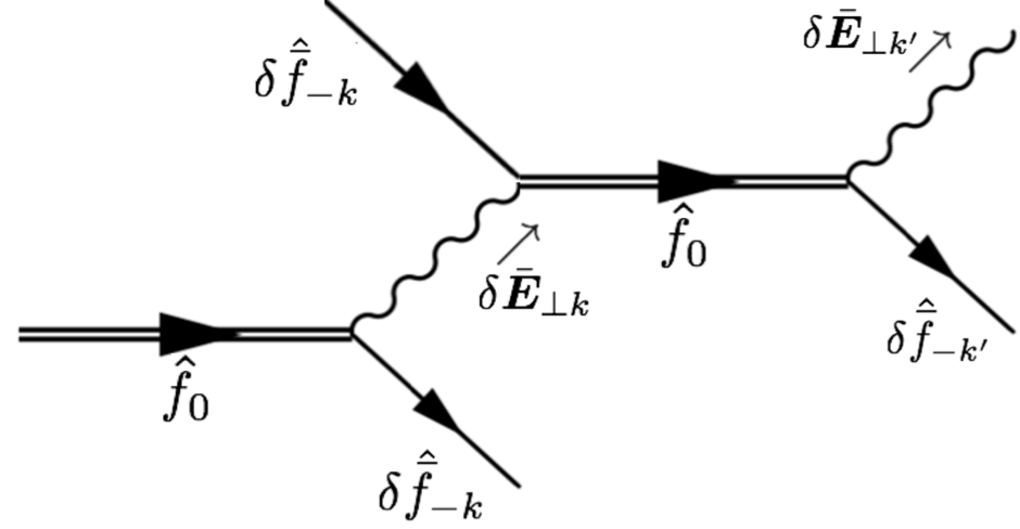
Figure 10: Diagrammatic representation of chorus chirping consistent with the “rules” introduced in Fig. 11. The renormalized response of supra-thermal electrons, represented by the double solid line propagator, is unstable and emits and re-absorbs same-$k$ fluctuations, which is the strongest nonlinear process on long times. Chorus chirping occurs because, at subsequent times, different $k$’s maximize wave particle power transfer (Zonca ., 2017).

The double solid line propagator represents the renormalized response of supra-thermal electrons, which is unstable and, thus, nonlinearly emits oscillators belonging to the whistler spectrum. Emission and re-absorption of the same-$k$ has the strongest cross section (Zonca, Chen, Briguglio, Fogaccia, Vlad  Wang, 2015; Zonca, Chen, Briguglio, Fogaccia, Milovanov ., 2015; L. Chen  Zonca, 2016). As time progresses, emissions are those that maximize wave particle power transfer and, thus, chirping occurs spontaneously.

The generality of the present theoretical approach goes well beyond the analytic derivation of (Vomvoridis ., 1982) result of chorus chirping. It provides the insights for reconciling the present interpretation of chorus chirping with that originally provided by (Omura  Nunn, 2011). It also addresses the physics underlying the evidence of a small nonlinear frequency shift compared with the dynamic range of chorus frequency sweeping, as recently noted by (Tsurutani ., 2020). Meanwhile, it illuminates the origin of chorus sub-elements being the nonlinear phase modulation analogous to the process introduced by (O’Neil, 1965).

The present theoretical approach also sheds light on the profound analogies of chorus chirping in space physics and similar non-perturbative frequency sweeping modes in fusion plasmas. In fact, the essential common elements are the narrow fluctuation spectrum of chirping modes that are resonantly excited from a dense background of waves by supra-thermal particles, which respond non-perturbatively to maximize wave particle power transfer (Zonca, Chen, Briguglio, Fogaccia, Vlad  Wang, 2015; L. Chen  Zonca, 2016).

Last but not least, this theoretical approach provides a direct proof of the one-on-one correspondence of chorus chirping with super-radiance in free electron lasers, noted first by (Zonca, Chen, Briguglio, Fogaccia, Vlad  Wang, 2015; L. Chen  Zonca, 2016). It is also worthwhile emphasizing that the theoretical approaches presented in this work have interesting possible applications to nonlinear phenomena in high power radiation devices such as gyrotron backwave oscillators, where they may not only be applied, but also yield in-depth understandings (SH. Chen  Chen, 2012, 2013).

Appendix A The chorus linear dispersion relation

Here, we briefly derive the liner dispersion relation for chorus fluctuations (Kennel  Petschek, 1966), emphasizing the properties that are used for discussing the nonlinear physics addressed in this work. Reconsider Eqs. (16) and (20), and cast them as follows

$$W(z,t,\omega)+i\Gamma(z,t,\omega) = \frac{\omega_{p}^{2}}{n\omega\partial D_{w}/\partial\omega}\left\langle\frac{v_{\perp}^{2}/2}{\Omega+kv_{\parallel}-\omega}\left[\frac{k}{\omega}\frac{\partial f_{0}}{\partial v_{\|}}+\left(1-\frac{kv_{\|}}{\omega}\right)\frac{1}{v_{\perp}}\frac{\partial f_{0}}{\partial v_{\perp}}\right]\right\rangle$$ (46)

$$= \frac{\omega(\Omega-\omega)^{2}}{n\Omega}\left\langle\frac{v_{\perp}^{2}/2}{\Omega+kv_{\parallel}-\omega}\left[\frac{k}{\omega}\frac{\partial f_{0}}{\partial v_{\|}}-\frac{2}{v_{\perp}^{2}}\left(1-\frac{kv_{\|}}{\omega}\right)f_{0}\right]\right\rangle\;,$$

where, in the second line, we have integrated by parts in $v_{\perp}$ and used Eq. (6) to make $\partial D_{w}/\partial\omega$ explicit, assuming $\omega^{2}/\omega_{p}^{2}\ll 1$ for simplicity (cf. Sec. 2.2). Using the initial (linear) expression for $f_{0}$ given in Eq. (21), the spatial dependence of density and thermal speeds are connected with the magnetic field non-uniformity by the condition that $f_{0}$ be a function of constants of motion ${\cal E}=v^{2}/2$ and $\mu=v_{\perp}^{2}/2B$. The exponent in the bi-Maxwellian is then written as

$$-\frac{\cal E}{w_{\parallel}^{2}}+\frac{\mu B_{e}}{w_{\perp e}^{2}}\frac{B}{B_{e}}\left(\frac{w_{\perp e}^{2}}{w_{\parallel}^{2}}-\frac{w_{\perp e}^{2}}{w_{\perp}^{2}}\right)\;.$$

For this to be constant for arbitrary ${\cal E}=v^{2}/2$ and $\mu=v_{\perp}^{2}/2B$, we need to set $w_{\parallel}=w_{\parallel e}$ and $w_{\perp}=\zeta w_{\perp e}$, with $\zeta^{-2}=1+A(1-B_{e}/B)=1+A\xi z^{2}/(1+\xi z^{2})$, as noted below Eq. (21). Furthermore, the pre-factor in the bi-Maxwellian is constant only if $n_{0}/n_{e}=w_{\perp}^{2}/w_{\perp e}^{2}=\zeta^{2}$. Meanwhile, performing the velocity space integration, it is possible to write

$$W(z,0,\omega)+i\Gamma(z,0,\omega) = \frac{n_{e}(\Omega-\omega)^{2}}{n\Omega}\zeta^{2}\left[1-(A+1)\zeta^{2}+(A+1)\zeta^{2}\frac{(\Omega-\omega)}{\sqrt{2}|k|w_{\parallel e}}Z\left(\frac{\omega-\Omega}{\sqrt{2}|k|w_{\parallel e}}\right)\right.$$ (47)

$$\left.-\frac{\Omega}{\sqrt{2}|k|w_{\parallel e}}Z\left(\frac{\omega-\Omega}{\sqrt{2}|k|w_{\parallel e}}\right)\right]\;.$$

Here, from Sec. 2.1, we have recalled $n_{0}=\zeta^{2}n_{e}$ and $Z(x)=\pi^{-1/2}\int_{-\infty}^{\infty}e^{-y^{2}}/(y-x)dy$ is the plasma dispersion function. Noting $A+1-\zeta^{-2}=A/(1+\xi z^{2})$, Eq. (47) can be rewritten as

$$W(z,0,\omega)+i\Gamma(z,0,\omega)=\frac{n_{e}(\Omega-\omega)^{2}}{n\Omega}\zeta^{4}\left[-\frac{A}{1+\xi z^{2}}+\frac{A\Omega_{e}-(A+1)\omega}{\sqrt{2}|k|w_{\parallel e}}Z\left(\frac{\omega-\Omega}{\sqrt{2}|k|w_{\parallel e}}\right)\right]\;.$$ (48)

This expression shows that $\omega/\Omega_{e}=A/(A+1)$ is the frequency where wave particle power exchange with hot electrons changes sign and the driving rate becomes a damping (Kennel  Petschek, 1966). Meanwhile, Eq. (48) also shows that $W(z,0,\omega)$ and $\Gamma(z,0,\omega)$ scale as $\zeta^{4}$. Thus, recalling from Sec. 2.1 that $\zeta^{-2}=1+A\xi z^{2}/(1+\xi z^{2})$, the length scale of the hot electron contribution to the chorus dispersion relation is $\sim(A\xi)^{-1/2}$, which, already at moderate values of $A$, rapidly takes over the non-uniformity due to the ambient magnetic field, that is $B=B_{e}(1+\xi z^{2})$ (Helliwell, 1967), as illustrated in Fig. 1. This suggests that formal simplification can be achieved in the analytical investigation of chorus nonlinear dynamics, addressed in this work, by assuming a non-uniform source of hot electrons, localized about the equator, neglecting, meanwhile, magnetic field non-uniformity. As noted in Sec. 2.1, this assumption, although not strictly necessary, helps simplifying the analytical derivations in this work; and can be formally obtained for $A\gg 1$. In fact, as noted above, the $\sim(A\xi)^{-1/2}$ length scale in the hot electron non-uniform response takes over the magnetic field non-uniformity already at moderate values of $A$.

Appendix B The Dyson-Schwinger equation approach

Here, we elaborate the Dyson-Schwinger equation approach presented in Refs. (L. Chen  Zonca, 2016; Zonca, Chen, Briguglio, Fogaccia, Vlad  Wang, 2015), with the applications to magnetized fusion plasma presented therein, specializing it to nonlinear dynamics and phase space transport by chorus emission.

The “Dyson-like equation” terminology, by analogy with the earlier work by (Al’Tshul’  Karpman, 1966), was introduced by (L. Chen  Zonca, 2016; Zonca, Chen, Briguglio, Fogaccia, Vlad  Wang, 2015) as a tribute to Freeman J. Dyson, who recently passed away (https://en.wikipedia.org/wiki/Freeman_Dyson). The Dyson-Schwinger equations, as equations of motion of Green functions, provide a complete description of the theory (Dyson, 1949), since they describe the propagation as well as interaction of the fields themselves. From this point of view, Dyson-Schwinger equations, and Eq. (33) as a particular case, can be used to generate perturbation expansions in the weak field limit, cf. Fig. 11 (b), but can also be adopted for the more general strong-coupling case.

The elementary process that underlies this dynamics is illustrated in Fig. 11 (a), where we have borrowed and suitably modified the Feynman diagram rules as in (L. Chen  Zonca, 2016; Zonca ., 2017) to illustrate Eq. (32) and its reverse. In particular, straight lines represent linearized propagators (Green functions) of particle distribution functions, while wavy lines stand for linearized propagators (Green functions) of fluctuating electromagnetic fields. Arrows indicate the direction of propagation. Meanwhile, nodes represent (nonlinear) interactions/couplings. Furthermore, because of energy and momentum conservation in particle and electromagnetic fields field interactions, propagation of fields is equivalent to the opposite propagation of corresponding complex conjugate fields (Zonca, Chen, Briguglio, Fogaccia, Milovanov ., 2015). For example, emission of $\delta\bar{E}_{k}$ corresponds to absorption of $\delta\bar{E}_{k}^{*}$ because of symmetry under parity and time reversal transformations. Thus, the left node (vertex) in Fig. 11 (a) represents (the $c.c.$ of) Eq. (32); while the right node (vertex) represents the first two lines of Eq. (33). In the present theoretical approach, emission and reabsorption of $\delta\bar{E}_{k}$ and $\delta\bar{E}_{k}^{*}$ can occur repeatedly. Here, by emission we mean “generation of waves” because of the instability driven by the spatially averaged electron distribution function $\hat{f}_{0}$. Meanwhile, by reabsorption we intend to mean the “nonlinear interaction” of electromagnetic fluctuations with the perturbed electron distribution function that modifies $\hat{f}_{0}$ itself. This is illustrated in the upper part of Fig. 11 (b) in the form of a Dyson series, and dominates the nonlinear dynamics since it can be shown to cause the most significant distortion of $\hat{f}_{0}$ on the long time scale (van Hove, 1954; Prigogine, 1962; Balescu, 1963; Al’Tshul’  Karpman, 1966; Dupree, 1966; Aamodt, 1967; Weinstock, 1969; Mima, 1973; Zonca, Chen, Briguglio, Fogaccia, Vlad  Wang, 2015; Zonca, Chen, Briguglio, Fogaccia, Milovanov ., 2015; L. Chen  Zonca, 2016; Zonca ., 2017). Such a distortion of the hot electron distribution function, determined self-consistently in the presence of the finite amplitude fluctuation spectrum, constitutes the “renormalized” hot electron response, denoted with the double solid line in Fig. 11 (b). It is this renormalized hot electron $\hat{f}_{0}$, which is evolving in time, that self-consistently causes the evolution of the fluctuation spectrum according to Eqs. (11) to (16) and as illustrated in the lower part of Fig. 11 (b).

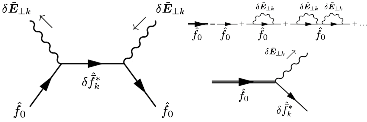
(a)                                                                 (b)

Figure 11: (a) Diagrammatic representation of the elementary processes of Eqs. (32) and (33). (b) Diagrammatic representation of the renormalized $\hat{f}_{0}$ hot electron response as solution of the Dyson-like equation (33).

Equation (33), meanwhile, is a nonlinear integro-differential equation and can be used to close the chorus wave equations discussed in Sec. 2.1. In fact, it describes the response of the $k=0$ hot electron distribution function by continuous emission and reabsorption of whistler waves, shown in Fig. 11 (b), which are amplified due to wave particle resonant interactions. Again, we note that this emission and reabsorption occur with any generic whistler wave packet as denoted by the summation over the whole fluctuation spectrum, which is evolving in time self-consistently with the $k=0$ particle distribution function. In this respect, as noted already, Eq. (33) can be viewed as the renormalized hot electron distribution function evolving on the nonlinear time scale, which justifies dubbing it as Dyson-like equation (L. Chen  Zonca, 2016; Zonca, Chen, Briguglio, Fogaccia, Vlad  Wang, 2015; Zonca, Chen, Briguglio, Fogaccia, Milovanov ., 2015).

Appendix C Detailed derivation of Eqs. (37) and (38).

C.1 Derivation of Eq. (37).

In this Appendix, we briefly summarize the derivation of Eq. (37) from Eq. (27) based on Eqs. (33) and (36). For consistency with Sec. 3, we also denote the current frequency and wave number satisfying the lowest order whistler wave dispersion relation as $\bar{\omega}$ and $\bar{k}$ in order to distinguish them from $\omega$ and $k$ in the running summation over the fluctuation spectrum. Formally, we can rewrite Eq. (27) as

$$\bar{W}(\bar{\omega})+i\bar{\Gamma}(\bar{\omega}) = \frac{n_{e}}{n}\left(1-\frac{v_{r\bar{\omega}}}{v_{g\bar{\omega}}}\right)^{2}\left\langle\frac{v_{\perp}^{2}}{2}\Omega_{e}\left[\Omega_{e}+\bar{k}v_{\parallel}-\bar{\omega}-i(1-v_{r\bar{\omega}}/v_{g\bar{\omega}})\partial_{t}\right]^{-1}\right.$$ (49)

$$\times\left.\left(\frac{\bar{k}}{\bar{\omega}}\frac{\partial}{\partial v_{\parallel}}-\frac{2}{v_{\perp}^{2}}\frac{\Omega_{e}}{\bar{\omega}}\right)\left(\partial_{t}+v_{\parallel}\partial_{z}\right)^{-1}\left(\partial_{t}+v_{\parallel}\partial_{z}\right)\hat{f}_{0}\right\rangle\;,$$

where, for brevity, we have omitted the dependences on $t-z/v_{g\bar{\omega}}$. From this, upon substitution of Eq. (33) and noting Eq. (36), we have

$$\bar{W}(\bar{\omega})+i\bar{\Gamma}(\bar{\omega}) = \frac{n_{e}}{n}\left(1-\frac{v_{r\bar{\omega}}}{v_{g\bar{\omega}}}\right)^{2}\left\langle\frac{v_{\perp}^{2}}{2}\Omega_{e}\left[\Omega_{e}+\bar{k}v_{\parallel}-\bar{\omega}-i(1-v_{r\bar{\omega}}/v_{g\bar{\omega}})\partial_{t}\right]^{-1}\right.$$ (50)

$$\times\left(\frac{\bar{k}}{\bar{\omega}}\frac{\partial}{\partial v_{\parallel}}-\frac{2}{v_{\perp}^{2}}\frac{\Omega_{e}}{\bar{\omega}}\right)\sum_{k}\frac{e^{2}}{2m^{2}}v_{\perp}|\delta\bar{E}_{k}|\left[\frac{k}{\omega}\frac{\partial}{\partial v_{\parallel}}+\left(1-\frac{kv_{\parallel}}{\omega}\right)\left(\frac{1}{v_{\perp}}\frac{\partial}{\partial v_{\perp}}+\frac{1}{v_{\perp}^{2}}\right)\right]$$

$$\times\left[(\Omega_{e}+kv_{\parallel}-\omega)^{2}+(1-v_{r\omega}/v_{g\omega})^{2}\partial_{t}^{2}\right]^{-1}(1-v_{r\omega}/v_{g\omega})\partial_{t}v_{\perp}|\delta\bar{E}_{k}|$$

$$\times\left.\left[\frac{k}{\omega}\frac{\partial}{\partial v_{\parallel}}+\left(1-\frac{kv_{\parallel}}{\omega}\right)\frac{1}{v_{\perp}}\frac{\partial}{\partial v_{\perp}}\right]\hat{f}_{0}\right\rangle$$

$$\simeq \frac{n_{e}}{n}\left(1-\frac{v_{r\bar{\omega}}}{v_{g\bar{\omega}}}\right)^{2}\left\langle\frac{v_{\perp}^{2}}{2}\Omega_{e}\left[\Omega_{e}+\bar{k}v_{\parallel}-\bar{\omega}-i(1-v_{r\bar{\omega}}/v_{g\bar{\omega}})\partial_{t}\right]^{-1}\right.$$

$$\times\left(\frac{\bar{k}}{\bar{\omega}}\frac{\partial}{\partial v_{\parallel}}-\frac{2}{v_{\perp}^{2}}\frac{\Omega_{e}}{\bar{\omega}}\right)\sum_{k}\frac{e^{2}}{2m^{2}}v_{\perp}|\delta\bar{E}_{k}|\left[\frac{k}{\omega}\frac{\partial}{\partial v_{\parallel}}+\frac{\Omega_{e}}{\omega}\left(\frac{1}{v_{\perp}}\frac{\partial}{\partial v_{\perp}}+\frac{1}{v_{\perp}^{2}}\right)\right]$$

$$\times\left[(\Omega_{e}+kv_{\parallel}-\omega)^{2}+(1-v_{r\omega}/v_{g\omega})^{2}\partial_{t}^{2}\right]^{-1}(1-v_{r\omega}/v_{g\omega})\partial_{t}v_{\perp}|\delta\bar{E}_{k}|$$

$$\times\left.\left[\frac{k}{\omega}\frac{\partial}{\partial v_{\parallel}}+\frac{\Omega_{e}}{\omega}\frac{1}{v_{\perp}}\frac{\partial}{\partial v_{\perp}}\right]\hat{f}_{0}\right\rangle\;.$$

To derive Eq. (37), the last step is to integrate by parts twice in $v_{\perp}$ in order to eliminate $\partial_{v_{\perp}}$, taking into account that

$$\left\langle v_{\perp}^{4}\hat{f}_{0}\right\rangle=2\frac{\left\langle v_{\perp}^{2}\hat{f}_{0}\right\rangle^{2}}{\left\langle\hat{f}_{0}\right\rangle}\;,$$ (51)

for the anisotropic Maxwellian of Eq. (21).

C.2 Derivation of Eq. (38).

Velocity space integration in Eq. (37) is naturally (and more rigorously) performed in the Laplace- rather than in the time-representation (L. Chen  Zonca, 2016; Zonca, Chen, Briguglio, Fogaccia, Vlad  Wang, 2015; Zonca ., 2017; Tao ., 2020). Here, however, for the sake of simplicity and conciseness, we directly manipulate Eq. (37) in the time-representation formally handling operator symbols. Let’s first note, considering Eq. (35),

$$\left[\Omega_{e}+\bar{k}v_{\parallel}-\bar{\omega}-i(1-v_{r\bar{\omega}}/v_{g\bar{\omega}})\partial_{t}\right]^{-1} \simeq \left[(\Omega_{e}+\bar{k}v_{\parallel}-\bar{\omega})^{2}+(1-v_{r\bar{\omega}}/v_{g\bar{\omega}})^{2}\partial_{t}^{2}\right]^{-1}$$ (52)

$$\times\left[\Omega_{e}+\bar{k}v_{\parallel}-\bar{\omega}+i(1-v_{r\bar{\omega}}/v_{g\bar{\omega}})\partial_{t}\right]$$

$$\simeq \left[x^{2}+a^{2}\right]^{-1}\left[x+ia\right]\;,$$

having denoted symbolically $x\equiv\bar{k}(v_{\parallel}-v_{r\bar{\omega}})$ and $a\equiv(1-v_{r\bar{\omega}}/v_{g\bar{\omega}})\partial_{t}$. Here, $a$ as an operator is meant to be acting on $|\delta\bar{E}_{\bar{k}}|$ and what follows in the representation of the integrand, that is $|\delta\bar{E}_{k}|^{2}$ and $\hat{f}_{0}$. In fact, in the derivation of Eqs. (20) and (25), we have normalized the wave particle power exchange to $|\delta\bar{E}_{\bar{k}}|^{2}$. Thus, the nonlinear frequency and wave number shift due to the incremental change in the wave packet amplitude and phase is reabsorbed into $\bar{k}(v_{\parallel}-v_{r\bar{\omega}})$ as will be further discussed below in Sec. 4. We can adopt the same symbolic representation for Eq. (36) and, thus,

$$\left[(\Omega_{e}+kv_{\parallel}-\omega)^{2}+(1-v_{r\omega}/v_{g\omega})^{2}\partial_{t}^{2}\right]^{-1}(1-v_{r\omega}/v_{g\omega})\partial_{t}\simeq\left[(x-x_{0})^{2}+b^{2}\right]^{-1}b\;,$$ (53)

where $x_{0}\equiv\omega-\bar{\omega}-v_{r\omega}(k-\bar{k})\simeq(1-v_{r\omega}/v_{g\omega})(\omega-\bar{\omega})$ and $b\equiv(1-v_{r\omega}/v_{g\omega})\partial_{t}$ as an operator is meant to be acting on $|\delta\bar{E}_{k}|$ and $\hat{f}_{0}$. Meanwhile, for resonant particles, we note that, for $\mathbb{R}ea>0,\mathbb{R}eb>0\text{ and }|a|,|b|,|x_{0}|\ll 1$

$$\left[x^{2}+a^{2}\right]^{-1}a\left[(x-x_{0})^{2}+b^{2}\right]^{-1}b \simeq (\pi/2)\left[x_{0}^{2}+(a+b)^{2}\right]^{-1}(a+b)\left(\delta(x)+\delta(x-x_{0})\right)$$

$$-(\pi/2)\left[x_{0}^{2}+(a-b)^{2}\right]^{-1}(a-b)\left(\delta(x)-\delta(x-x_{0})\right)\;,$$

inside the velocity space integrand; and

$$\left[x^{2}+a^{2}\right]^{-1}x\left[(x-x_{0})^{2}+b^{2}\right]^{-1}b \simeq (\pi/2)\left[x_{0}^{2}+(a+b)^{2}\right]^{-1}x_{0}\left(\delta(x)+\delta(x-x_{0})\right)$$

$$-(\pi/2)\left[x_{0}^{2}+(a-b)^{2}\right]^{-1}x_{0}\left(\delta(x)-\delta(x-x_{0})\right)\;.$$

Terms depending on $\delta(x)$ in the velocity space integrand are computed at $v_{\parallel}=v_{r\omega}$, while those depending on $\delta(x-x_{0})$ are computed at $v_{\parallel}=v_{r\bar{\omega}}$. We can further simplify these expressions noting that, for a narrow spectrum, contributions $\propto\left(\delta(x)-\delta(x-x_{0})\right)$ can be neglected. Furthermore, the symbolic expression of $(a+b)$ can also be simplified noting assumption (i) above and, thus

$$(a+b) \simeq |\delta\bar{E}_{k}|^{-3}\hat{f}_{0}^{-1}(1-v_{r\omega}/v_{g\omega})\partial_{t}|\delta\bar{E}_{k}|^{3}\hat{f}_{0}$$ (56)

$$+|\delta\bar{E}_{k}|^{-1}\hat{f}_{0}^{-1}(1-v_{r\omega}/v_{g\omega})\partial_{t}|\delta\bar{E}_{k}|\hat{f}_{0}$$

$$\simeq 2|\delta\bar{E}_{k}|^{-2}\hat{f}_{0}^{-1}(1-v_{r\omega}/v_{g\omega})\partial_{t}|\delta\bar{E}_{k}|^{2}\hat{f}_{0}\;.$$

Again, these symbolic relations are more rigorously interpreted in the Laplace- rather than the time-representation (L. Chen  Zonca, 2016; Zonca, Chen, Briguglio, Fogaccia, Vlad  Wang, 2015; Zonca ., 2017; Tao ., 2020). Interested readers are referred to the original references for more details.

Based on these relations, one can derive Eqs. (38) and (39), where we have noted that

$$\frac{1}{k}\frac{\partial}{\partial v_{r\omega}}=\frac{1}{(1-v_{r\omega}/v_{g\omega})}\frac{\partial}{\partial\omega}\;,$$ (57)

justifying the usefulness of introducing the normalization of $\bar{W}$ and $\bar{\Gamma}$ as in Eq. (27) in Sec. 2.2. The presence of the integral operator

$$\left[\frac{\left(\omega-\bar{\omega}\right)^{2}}{4\Omega_{e}^{2}}+\Omega_{e}^{-2}\partial_{t}^{2}\right]^{-1}$$ (58)

is what allows us to neglect the non-resonant particle response (Cauchy principal value) in the derivations above.

Appendix D Evolution equations for numerical solution of the reduced Dyson-like equation.

To exploit the dense nature of the whistler wave spectrum, we introduce the dimensionless intensity ${\cal I}(\omega)$ such that

$$\sum_{k}\frac{\left\langle\left\langle\omega_{{\rm tr}k}^{4}\right\rangle\right\rangle}{\Omega_{e}^{4}}=\frac{\hat{\gamma}_{e}^{2}}{\Omega_{e}^{2}}\int\frac{d\omega}{\Omega_{e}}{\cal I}(\omega)\frac{\omega^{3/2}}{(\Omega_{e}-\omega)^{3/2}}\;.$$ (59)

Here, the $\omega^{3/2}/(\Omega_{e}-\omega)^{3/2}$ factor accounts for the $\sim I_{k}k^{3}$ scaling of $\left\langle\left\langle\omega_{{\rm tr}k}^{4}\right\rangle\right\rangle$. This normalization is chosen ad hoc to have nonlinearity effects being important when ${\cal I}(\omega)\sim{\cal O}(1)$.

To invert the integral operator of Eq. (58), let us introduce the auxiliary functions

$$\left[\frac{\left(\omega-\bar{\omega}\right)^{2}}{4\Omega_{e}^{2}}+\Omega_{e}^{-2}\partial_{t}^{2}\right]G_{L1}(\omega,\bar{\omega})=\frac{\hat{\gamma}_{e}^{2}}{\Omega_{e}^{2}}\frac{{\cal I}(\omega)}{(1-v_{r\omega}/v_{g\omega})^{4}}\bar{\Gamma}_{L}(\omega)\;,$$

$$\left[\frac{\left(\omega-\bar{\omega}\right)^{2}}{4\Omega_{e}^{2}}+\Omega_{e}^{-2}\partial_{t}^{2}\right]G_{L2}(\omega,\bar{\omega})=\frac{\hat{\gamma}_{e}^{2}}{\Omega_{e}^{2}}\frac{{\cal I}(\omega)}{(1-v_{r\omega}/v_{g\omega})^{4}}\bar{\Gamma}_{L}(\bar{\omega})\;,$$

$$\left[\frac{\left(\omega-\bar{\omega}\right)^{2}}{4\Omega_{e}^{2}}+\Omega_{e}^{-2}\partial_{t}^{2}\right]G_{NL1}(\omega,\bar{\omega})=\frac{\hat{\gamma}_{e}^{2}}{\Omega_{e}^{2}}\frac{{\cal I}(\omega)}{(1-v_{r\omega}/v_{g\omega})^{4}}\bar{\Gamma}_{NL}(\omega)\;,$$

$$\left[\frac{\left(\omega-\bar{\omega}\right)^{2}}{4\Omega_{e}^{2}}+\Omega_{e}^{-2}\partial_{t}^{2}\right]G_{NL2}(\omega,\bar{\omega})=\frac{\hat{\gamma}_{e}^{2}}{\Omega_{e}^{2}}\frac{{\cal I}(\omega)}{(1-v_{r\omega}/v_{g\omega})^{4}}\bar{\Gamma}_{NL}(\bar{\omega})\;;$$ (60)

where, from Eq. (39),

$$\bar{\Gamma}_{NL}(\bar{\omega}) = \left[\Omega_{e}\frac{\partial}{\partial\bar{\omega}}-\frac{2\Omega_{e}^{2}}{\bar{k}^{2}\left\langle v_{\perp}^{2}\right\rangle}\left(1-\frac{v_{r\bar{\omega}}}{v_{g\bar{\omega}}}\right)\right]\Omega_{e}\frac{\partial}{\partial\bar{\omega}}\int\frac{d\omega}{\Omega_{e}}\frac{\omega^{3/2}}{(\Omega_{e}-\omega)^{3/2}}$$ (61)

$$\times\frac{1}{8}\left[G_{L1}(\omega,\bar{\omega})+G_{L2}(\omega,\bar{\omega})+G_{NL1}(\omega,\bar{\omega})+G_{NL2}(\omega,\bar{\omega})\right]\;.$$

Meanwhile, Eq. (38) can be cast as

$$\Omega_{e}^{-1}\partial_{t}\bar{W}(\bar{\omega}) = \left[\Omega_{e}\frac{\partial}{\partial\bar{\omega}}-\frac{2\Omega_{e}^{2}}{\bar{k}^{2}\left\langle v_{\perp}^{2}\right\rangle}\left(1-\frac{v_{r\bar{\omega}}}{v_{g\bar{\omega}}}\right)\right]\Omega_{e}\frac{\partial}{\partial\bar{\omega}}\int\frac{d\omega}{\Omega_{e}}\frac{\omega^{3/2}}{(\Omega_{e}-\omega)^{3/2}}\frac{\left(\omega-\bar{\omega}\right)}{2\Omega_{e}}$$ (62)

$$\times\frac{1}{8}\left[G_{L1}(\omega,\bar{\omega})+G_{L2}(\omega,\bar{\omega})+G_{NL1}(\omega,\bar{\omega})+G_{NL2}(\omega,\bar{\omega})\right]\;.$$

Equations (60) to (62) are closed by the intensity evolution equation,

$$\Omega_{e}^{-1}\partial_{t}{\cal I}(\omega) = 2{\cal S}{\cal I}(\omega)^{1/2}+2{\cal I}(\omega)\frac{\omega(\Omega_{e}-\omega)^{2}}{\Omega_{e}^{3}}\left[\partial_{t}\left(\int_{z-v_{g\omega}t}^{\infty}\zeta^{4}(z^{\prime})\frac{dz^{\prime}}{v_{g\omega}}\right)\bar{\Gamma}(\omega)\right.$$ (63)

$$\left.\left.+\left(\int_{z-v_{g\omega}t}^{\infty}\zeta^{4}(z^{\prime})\frac{dz^{\prime}}{v_{g\omega}}\right)\partial_{t}\bar{\Gamma}(\omega)\right]\right/\left(1-\frac{v_{r\omega}}{v_{g\omega}}\right)^{2}\;;$$

and the wave packet phase evolution equation,

$$\Omega_{e}^{-1}\partial_{t}\varphi(\omega) = -\frac{\omega(\Omega_{e}-\omega)^{2}}{\Omega_{e}^{3}}\left[\partial_{t}\left(\int_{z-v_{g\omega}t}^{\infty}\zeta^{4}(z^{\prime})\frac{dz^{\prime}}{v_{g\omega}}\right)\bar{W}(\omega)\right.$$ (64)

$$\left.\left.+\left(\int_{z-v_{g\omega}t}^{\infty}\zeta^{4}(z^{\prime})\frac{dz^{\prime}}{v_{g\omega}}\right)\partial_{t}\bar{W}(\omega)\right]\right/\left(1-\frac{v_{r\omega}}{v_{g\omega}}\right)^{2}\;;$$

which can be readily derived from Eqs. (11) and (14) keeping in mind the discussion given in the first paragraph of Sec. 3. Note that we have added a source term $2{\cal S}{\cal I}(\omega)^{1/2}$ on the right hand side of Eq. (63). The value of ${\cal S}$ represents the injection rate of fluctuations in the $|\delta\bar{E}_{k}|$ spectrum. We adopted it because it gives us a variety of possibilities rather than assuming an initial spectrum; e.g., using ${\cal S}$ as a random source stirring the system or a constant uniform source. Figure 12 gives a comparison of the linear evolution of ${\cal I}(z=50c/\omega_{e},t,\omega)$ in the case of a random (a) and uniform source (b) of the same strength ${\cal S}=2\times 10^{-5}$. Parameters are the same as in Fig. 1. In both cases, we clearly note the predominance of a narrow spectrum at the most unstable frequency after the whistler wave packet has been convectively amplified by crossing the localized hot electron source at the equator. Because of this, we will focus on the uniform source case in the following, and discuss random or more general sources in later studies.

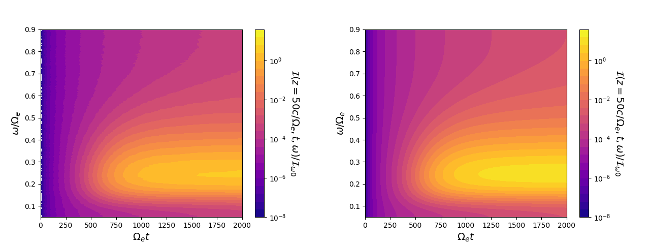
(a)                                                                 (b)

Figure 12: Contour plot of the linear evolution of ${\cal I}(z=50c/\omega_{e},t,\omega)$ for (a) a random source and (b) a uniform source of the same strength ${\cal S}=2\times 10^{-5}$ in Eq. (63). The position is fixed at $z\Omega_{e}/c=50$ and parameters are the same as in Fig. 1.

Equations (60) to (64) fully characterize the self-consistent nonlinear evolution of a whistler wave packet spectrum excited by wave particle resonances with a hot electron source that is localized about the equator. As anticipated in Secs. 2.2 and 3, they assume that the whistler wave packets belong to a dense (nearly continuous) spectrum that are continuously emitted and reabsorbed (cf. Fig. 11 and corresponding discussion) to maximize wave particle power transfer (L. Chen  Zonca, 2016; Zonca, Chen, Briguglio, Fogaccia, Vlad  Wang, 2015). When solving these equations by advancing them in time by one step $\Delta t$, one has to keep in mind that the wave packet amplitude and phase are shifted nonlinearly and cause hot electron induced frequency ($\Delta(\Delta_{\omega})=-\Delta t\partial_{t}^{2}\varphi(\omega)$) and corresponding wave number shifts, introduced in Sec. 2.2. Despite $\Delta_{\omega}/\Delta_{k}=v_{g\omega}$, and, thus, the shifted wave packet still satisfies the whistler dispersion relation, the hot electron induced phase shift causes a corresponding small but finite shift in the resonant velocity $k\Delta v_{r\omega}=\Delta_{\omega}-v_{r\omega}\Delta_{k}=(1-v_{r\omega}/v_{g\omega})\Delta_{\omega}$. This means that, after advancing in time by one step $\Delta t$, the functions $\bar{\Gamma}_{NL}$ and $\bar{W}_{NL}$ are actually evaluated at $\bar{\omega}+\Delta(\Delta_{\omega})$. Thus, noting Eq. (57), these functions have to be updated as

$$\bar{\Gamma}_{NL}(\bar{\omega}) \rightarrow \bar{\Gamma}_{NL}(\bar{\omega})-\Delta(\Delta_{\omega})\frac{\partial}{\partial\bar{\omega}}\bar{\Gamma}_{NL}(\bar{\omega})\;,$$

$$\bar{W}_{NL}(\bar{\omega}) \rightarrow \bar{W}_{NL}(\bar{\omega})-\Delta(\Delta_{\omega})\frac{\partial}{\partial\bar{\omega}}\bar{W}_{NL}(\bar{\omega})\;.$$ (65)

A similar argument applies to ${\cal I}(\omega)$ and $\varphi(\omega)$, such that

$${\cal I}(\omega) \rightarrow {\cal I}(\omega)-\Delta(\Delta_{\omega})\frac{\partial}{\partial\omega}{\cal I}(\omega)\;,$$

$$\varphi(\omega) \rightarrow \varphi(\omega)-\Delta(\Delta_{\omega})\frac{\partial}{\partial\omega}\varphi(\omega)\;;$$ (66)

after each time step. Note that Eq. (66) corresponds to changing $\partial_{t}\rightarrow\partial_{t}-\partial_{t}^{2}\varphi(\omega)\partial_{\omega}$ on the left hand side of Eqs. (63) and (64); that is, to solving the wave kinetic equation (Bernstein  Baldwin, 1977; McDonald, 1988) for wave packet intensity and phase.

Considering ${\cal I}(\omega)=0$ together with $\varphi(\omega)=0$ at $t=0$, initial conditions for Eqs. (60) are particularly simple:

$$\left.G_{...}(\omega,\bar{\omega})\right|_{t=0} = 0\;,$$

$$\left.\partial_{t}G_{...}(\omega,\bar{\omega})\right|_{t=0} = 0\;;$$ (67)

where, for brevity, we have generically denoted by $\ldots$ the subscripts of $G_{...}(\omega,\bar{\omega})$ functions defined in Eqs. (60). Furthermore, for Eqs. (61) and (62),

$$\left.\bar{\Gamma}_{NL}(\omega)\right|_{t=0} = 0\;,$$

$$\left.\bar{W}_{NL}(\omega)\right|_{t=0} = 0\;.$$ (68)

Finally, considering a frequency domain such that the fluctuation spectrum at the boundary is sufficiently small that it can be neglected, boundary conditions are the trivial ones; i.e., $G_{...}(\omega,\bar{\omega})$ functions, $\bar{\Gamma}_{NL}(\omega)$ and $\bar{W}_{NL}(\omega)$ vanish at any time. However, more realistically and to avoid undesirable discontinuities at the boundary of the frequency simulation domain, we assume that values at the boundaries are obtained by linear extrapolation of the inner solution.

References

- Aamodt (\APACyear1967) \APACinsertmetastarAamodt1967{APACrefauthors}Aamodt, R\BPBIE. \APACrefYearMonthDay1967. \BBOQ\APACrefatitleTest Waves in Weakly Turbulent Plasmas Test waves in weakly turbulent plasmas.\BBCQ \APACjournalVolNumPagesThe Physics of Fluids1061245-1250. {APACrefDOI} \doi10.1063/1.1762269 \PrintBackRefs\CurrentBib
- Al’Tshul’ \BBA Karpman (\APACyear1966) \APACinsertmetastarAltshul1966{APACrefauthors}Al’Tshul’, L\BPBIM.\BCBT \BBA Karpman, V\BPBII. \APACrefYearMonthDay1966\APACmonth02. \BBOQ\APACrefatitleTheory of Nonlinear Oscillations in a Collisionless Plasma Theory of nonlinear oscillations in a collisionless plasma.\BBCQ \APACjournalVolNumPagesJ. Exptl. Theoret. Phys. (U.S.S.R.)22361-369. \PrintBackRefs\CurrentBib
- Balescu (\APACyear1963) \APACinsertmetastarBalescu1963{APACrefauthors}Balescu, R. \APACrefYear1963. \APACrefbtitleStatistical Mechanics of Charged Particles Statistical mechanics of charged particles. \APACaddressPublisherInterscience, New York (USA). \PrintBackRefs\CurrentBib
- Bernstein \BBA Baldwin (\APACyear1977) \APACinsertmetastarBernstein1977{APACrefauthors}Bernstein, I\BPBIB.\BCBT \BBA Baldwin, D\BPBIE. \APACrefYearMonthDay1977. \BBOQ\APACrefatitleGeometric optics in space and time varying plasmas. II Geometric optics in space and time varying plasmas. ii.\BBCQ \APACjournalVolNumPagesThe Physics of Fluids201116-126. {APACrefURL} https://aip.scitation.org/doi/abs/10.1063/1.861700 {APACrefDOI} \doi10.1063/1.861700 \PrintBackRefs\CurrentBib
- Bortnik \BBA Thorne (\APACyear2007) \APACinsertmetastarBortnik2007c{APACrefauthors}Bortnik, J.\BCBT \BBA Thorne, R. \APACrefYearMonthDay2007. \BBOQ\APACrefatitleThe dual role of ELF/VLF chorus waves in the acceleration and precipitation of radiation belt electrons The dual role of ELF/VLF chorus waves in the acceleration and precipitation of radiation belt electrons.\BBCQ \APACjournalVolNumPagesJ. Atmos. Solar Terres. Phys.69378-386. {APACrefDOI} \doi10.1016/j.jastp.2006.05.030 \PrintBackRefs\CurrentBib
- Burtis \BBA Helliwell (\APACyear1976) \APACinsertmetastarBurtis1976{APACrefauthors}Burtis, W\BPBIJ.\BCBT \BBA Helliwell, R\BPBIA. \APACrefYearMonthDay1976. \BBOQ\APACrefatitleMagnetospheric chorus: Occurrence patterns and normalized frequency Magnetospheric chorus: Occurrence patterns and normalized frequency.\BBCQ \APACjournalVolNumPagesPlanet. Space Sci.24111007-1010. {APACrefDOI} \doi10.1016/0032-0633(76)90119-7 \PrintBackRefs\CurrentBib
- L. Chen \BBA Zonca (\APACyear2016) \APACinsertmetastarChen2016{APACrefauthors}Chen, L.\BCBT \BBA Zonca, F. \APACrefYearMonthDay2016Mar. \BBOQ\APACrefatitlePhysics of Alfvén waves and energetic particles in burning plasmas Physics of Alfvén waves and energetic particles in burning plasmas.\BBCQ \APACjournalVolNumPagesRev. Mod. Phys.88015008. {APACrefDOI} \doi10.1103/RevModPhys.88.015008 \PrintBackRefs\CurrentBib
- S\BHBIH. Chen \BBA Chen (\APACyear2012) \APACinsertmetastarSChen2012{APACrefauthors}Chen, S\BHBIH.\BCBT \BBA Chen, L. \APACrefYearMonthDay2012. \BBOQ\APACrefatitleLinear and nonlinear behaviors of gyrotron backward wave oscillators Linear and nonlinear behaviors of gyrotron backward wave oscillators.\BBCQ \APACjournalVolNumPagesPhys. Plasmas19023116. {APACrefDOI} \doidoi.org/10.1063/1.3688892 \PrintBackRefs\CurrentBib
- S\BHBIH. Chen \BBA Chen (\APACyear2013) \APACinsertmetastarSChen2013{APACrefauthors}Chen, S\BHBIH.\BCBT \BBA Chen, L. \APACrefYearMonthDay2013. \BBOQ\APACrefatitleNonstationary oscillation of gyrotron backward wave oscillators with cylindrical interaction structure Nonstationary oscillation of gyrotron backward wave oscillators with cylindrical interaction structure.\BBCQ \APACjournalVolNumPagesPhys. Plasmas20123108. {APACrefDOI} \doidx.doi.org/10.1063/1.4846876 \PrintBackRefs\CurrentBib
- Y. Chen \BOthers. (\APACyear2007) \APACinsertmetastarChen2007{APACrefauthors}Chen, Y., Reeves, G\BPBID.\BCBL \BBA Friedel, R\BPBIH\BPBIW. \APACrefYearMonthDay2007. \BBOQ\APACrefatitleThe energization of relativistic electrons in the outer Van Allen radiation belt The energization of relativistic electrons in the outer Van Allen radiation belt.\BBCQ \APACjournalVolNumPagesNature Physics. {APACrefDOI} \doidoi:10.1038/nphys655 \PrintBackRefs\CurrentBib
- Crabtree \BOthers. (\APACyear2017) \APACinsertmetastarCrabtree2017{APACrefauthors}Crabtree, C., Tejero, E., Ganguli, G., Hospodarsky, G\BPBIB.\BCBL \BBA Kletzing, C\BPBIA. \APACrefYearMonthDay2017. \BBOQ\APACrefatitleBayesian spectral analysis of chorus subelements from the Van Allen Probes Bayesian spectral analysis of chorus subelements from the Van Allen Probes.\BBCQ \APACjournalVolNumPagesJ. Geophys. Res. Space Physics12266088–6106. {APACrefDOI} \doi10.1002/2016JA023547 \PrintBackRefs\CurrentBib
- Cully \BOthers. (\APACyear2011) \APACinsertmetastarCully2011{APACrefauthors}Cully, C\BPBIM., Angelopoulos, V., Auster, U., Bonnell, J.\BCBL \BBA Le Contel, O. \APACrefYearMonthDay2011. \BBOQ\APACrefatitleObservational evidence of the generation mechanism for rising-tone chorus Observational evidence of the generation mechanism for rising-tone chorus.\BBCQ \APACjournalVolNumPagesGeophys. Res. Lett.38L01106. {APACrefDOI} \doi10.1029/2010GL045793 \PrintBackRefs\CurrentBib
- Demekhov (\APACyear2011) \APACinsertmetastarDemekhov2011{APACrefauthors}Demekhov, A. \APACrefYearMonthDay2011. \BBOQ\APACrefatitleGeneration of VLF emissions with the increasing and decreasing frequency in the magnetospheric cyclotron maser in the backward wave oscillator regime Generation of VLF emissions with the increasing and decreasing frequency in the magnetospheric cyclotron maser in the backward wave oscillator regime.\BBCQ \APACjournalVolNumPagesRadiophys. Quantum El.53609. {APACrefDOI} \doihttps://doi.org/10.1007/s11141-011-9256-x \PrintBackRefs\CurrentBib
- Dupree (\APACyear1966) \APACinsertmetastarDupree1966{APACrefauthors}Dupree, T\BPBIH. \APACrefYearMonthDay1966. \BBOQ\APACrefatitleA Perturbation Theory for Strong Plasma Turbulence A perturbation theory for strong plasma turbulence.\BBCQ \APACjournalVolNumPagesPhys. Fluids991773-1782. {APACrefDOI} \doi10.1063/1.1761932 \PrintBackRefs\CurrentBib
- Dyson (\APACyear1949) \APACinsertmetastarDyson1949{APACrefauthors}Dyson, F\BPBIJ. \APACrefYearMonthDay1949Jun. \BBOQ\APACrefatitleThe Matrix in Quantum Electrodynamics The matrix in quantum electrodynamics.\BBCQ \APACjournalVolNumPagesPhys. Rev.751736–1755. {APACrefURL} https://link.aps.org/doi/10.1103/PhysRev.75.1736 {APACrefDOI} \doi10.1103/PhysRev.75.1736 \PrintBackRefs\CurrentBib
- Hanzelka \BOthers. (\APACyear2020) \APACinsertmetastarHanzelka2020{APACrefauthors}Hanzelka, M., Santolík, O., Omura, Y., Kolmasová, I.\BCBL \BBA Kletzing, C\BPBIA. \APACrefYearMonthDay2020. \BBOQ\APACrefatitleA Model of the Subpacket Structure of Rising Tone Chorus Emissions A model of the subpacket structure of rising tone chorus emissions.\BBCQ \APACjournalVolNumPagesJ. Geophys. Res.125e2020JA028094. {APACrefDOI} \doidoi.org/10.1029/2020JA028094 \PrintBackRefs\CurrentBib
- Helliwell (\APACyear1967) \APACinsertmetastarHelliwell1967{APACrefauthors}Helliwell, R\BPBIA. \APACrefYearMonthDay1967. \BBOQ\APACrefatitleA theory of discrete VLF emissions from the magnetosphere A theory of discrete VLF emissions from the magnetosphere.\BBCQ \APACjournalVolNumPagesJ. Geophys. Res.72194773-4790. \PrintBackRefs\CurrentBib
- Hikishima \BBA Omura (\APACyear2012) \APACinsertmetastarHikishima2012{APACrefauthors}Hikishima, M.\BCBT \BBA Omura, Y. \APACrefYearMonthDay2012. \BBOQ\APACrefatitleParticle simulations of whistler-mode rising-tone emissions triggered by waves with different amplitudes Particle simulations of whistler-mode rising-tone emissions triggered by waves with different amplitudes.\BBCQ \APACjournalVolNumPagesJ. Geophys. Res.117A04226. {APACrefDOI} \doi10.1029/2011JA017428 \PrintBackRefs\CurrentBib
- Horne \BBA Thorne (\APACyear1998) \APACinsertmetastarHorne1998{APACrefauthors}Horne, R\BPBIB.\BCBT \BBA Thorne, R\BPBIM. \APACrefYearMonthDay1998. \BBOQ\APACrefatitlePotential waves for relativistic electron scattering and stochastic acceleration during magnetic storms Potential waves for relativistic electron scattering and stochastic acceleration during magnetic storms.\BBCQ \APACjournalVolNumPagesGeophys. Res. Lett.25153011-3014. \PrintBackRefs\CurrentBib
- Horne \BOthers. (\APACyear2005) \APACinsertmetastarHorne2005b{APACrefauthors}Horne, R\BPBIB., Thorne, R\BPBIM., Shprits, Y\BPBIY., Meredith, N\BPBIP., Glauert, S\BPBIA., Smith, A\BPBIJ.\BDBLDecreau, P\BPBIM\BPBIE. \APACrefYearMonthDay2005. \BBOQ\APACrefatitleWave acceleration of electrons in the Van Allen radiation belts Wave acceleration of electrons in the Van Allen radiation belts.\BBCQ \APACjournalVolNumPagesNature437227-230. {APACrefDOI} \doi10.1038/nature03939 \PrintBackRefs\CurrentBib
- Itzykson \BBA J.-B. Zuber (\APACyear1980) \APACinsertmetastarItzykson80{APACrefauthors}Itzykson, C.\BCBT \BBA J.-B. Zuber. \APACrefYear1980. \APACrefbtitleQuantum field theory Quantum field theory. \APACaddressPublisherNew YorkMcGraw-Hill. \PrintBackRefs\CurrentBib
- Katoh \BBA Omura (\APACyear2011) \APACinsertmetastarKatoh2011a{APACrefauthors}Katoh, Y.\BCBT \BBA Omura, Y. \APACrefYearMonthDay2011. \BBOQ\APACrefatitleAmplitude dependence of frequency sweep rates of whistler mode chorus emissions Amplitude dependence of frequency sweep rates of whistler mode chorus emissions.\BBCQ \APACjournalVolNumPagesJ. Geophys. Res.116A07201. {APACrefDOI} \doi10.1029/2011JA016496 \PrintBackRefs\CurrentBib
- Katoh \BBA Omura (\APACyear2013) \APACinsertmetastarKatoh2013{APACrefauthors}Katoh, Y.\BCBT \BBA Omura, Y. \APACrefYearMonthDay2013. \BBOQ\APACrefatitleEffect of the background magnetic field inhomogeneity on generation processes of whistler-mode chorus and broadband hiss-like emissions Effect of the background magnetic field inhomogeneity on generation processes of whistler-mode chorus and broadband hiss-like emissions.\BBCQ \APACjournalVolNumPagesJ. Geophys. Res.1184189-4198. {APACrefDOI} \doi10.1002/jgra.50395 \PrintBackRefs\CurrentBib
- Katoh \BBA Omura (\APACyear2016) \APACinsertmetastarKatoh2016{APACrefauthors}Katoh, Y.\BCBT \BBA Omura, Y. \APACrefYearMonthDay2016. \BBOQ\APACrefatitleElectron hybrid code simulation of whistler-mode chorus generation with real parameters in the Earth’s inner magnetosphere Electron hybrid code simulation of whistler-mode chorus generation with real parameters in the earth’s inner magnetosphere.\BBCQ \APACjournalVolNumPagesEarth, Planets, and Space68192. {APACrefDOI} \doihttps://doi.org/10.1186/s40623-016-0568-0 \PrintBackRefs\CurrentBib
- Kennel \BBA Petschek (\APACyear1966) \APACinsertmetastarKennel1966b{APACrefauthors}Kennel, C\BPBIF.\BCBT \BBA Petschek, H\BPBIE. \APACrefYearMonthDay1966. \BBOQ\APACrefatitleLimit on stably trapped particle fluxes Limit on stably trapped particle fluxes.\BBCQ \APACjournalVolNumPagesJ. Geophys. Res.7111-28. \PrintBackRefs\CurrentBib
- Li \BOthers. (\APACyear2011) \APACinsertmetastarLi2011{APACrefauthors}Li, W., Thorne, R\BPBIM., Bortnik, J., Shprits, Y\BPBIY., Nishimura, Y., Angelopoulos, V.\BDBLBonnell, J\BPBIW. \APACrefYearMonthDay2011. \BBOQ\APACrefatitleTypical properties of rising and falling tone chorus waves Typical properties of rising and falling tone chorus waves.\BBCQ \APACjournalVolNumPagesGeophys. Res. Lett.38L14103. {APACrefDOI} \doi10.1029/2011GL047925 \PrintBackRefs\CurrentBib
- Macúšová \BOthers. (\APACyear2010) \APACinsertmetastarMacusova2010{APACrefauthors}Macúšová, E., Santolík, O., P.Décréau, Demekhov, A\BPBIG., Nunn, D., Gurnett, D\BPBIA.\BDBLTrotignon, J\BHBIG. \APACrefYearMonthDay2010. \BBOQ\APACrefatitleObservations of the relationship between frequency sweep rates of chorus wave packets and plasma density Observations of the relationship between frequency sweep rates of chorus wave packets and plasma density.\BBCQ \APACjournalVolNumPagesJ. Geophys. Res.115A12257. {APACrefDOI} \doi10.1029/2010JA015468 \PrintBackRefs\CurrentBib
- McDonald (\APACyear1988) \APACinsertmetastarMcDonald1988{APACrefauthors}McDonald, S\BPBIW. \APACrefYearMonthDay1988. \BBOQ\APACrefatitlePhase-space representations of wave equations with applications to the eikonal approximation for short-wavelength waves Phase-space representations of wave equations with applications to the eikonal approximation for short-wavelength waves.\BBCQ \APACjournalVolNumPagesPhysics Reports1586337 - 416. {APACrefURL} http://www.sciencedirect.com/science/article/pii/0370157388900129 {APACrefDOI} \doihttps://doi.org/10.1016/0370-1573(88)90012-9 \PrintBackRefs\CurrentBib
- Mima (\APACyear1973) \APACinsertmetastarMima1973{APACrefauthors}Mima, K. \APACrefYearMonthDay1973. \BBOQ\APACrefatitleModification of Weak Turbulence Theory Due to Perturbed Orbit Effects. I. General Formulation Modification of weak turbulence theory due to perturbed orbit effects. i. general formulation.\BBCQ \APACjournalVolNumPagesJournal of the Physical Society of Japan3461620-1632. \PrintBackRefs\CurrentBib
- Miyoshi \BOthers. (\APACyear2010) \APACinsertmetastarMiyoshi2010{APACrefauthors}Miyoshi, Y., Katoh, Y., Nishiyama, T., Sakanoi, T., Asamura, K.\BCBL \BBA Hirahara, M. \APACrefYearMonthDay2010. \BBOQ\APACrefatitleTime of flight analysis of pulsating aurora electrons, considering wave-particle interactions with propagating whistler mode waves Time of flight analysis of pulsating aurora electrons, considering wave-particle interactions with propagating whistler mode waves.\BBCQ \APACjournalVolNumPagesJ. Geophys. Res.115A10312. {APACrefDOI} \doi10.1029/2009JA015127 \PrintBackRefs\CurrentBib
- Mourenas \BOthers. (\APACyear2015) \APACinsertmetastarMourenas2015{APACrefauthors}Mourenas, D., Artemyev, A\BPBIV., Agapitov, O\BPBIV., Krasnoselskikh, V.\BCBL \BBA Mozer, F\BPBIS. \APACrefYearMonthDay2015. \BBOQ\APACrefatitleVery oblique whistler generation by low-energy electron streams Very oblique whistler generation by low-energy electron streams.\BBCQ \APACjournalVolNumPagesJ. Geophys. Res. Space Physics12053665-3683. {APACrefDOI} \doi10.1002/2015JA021135 \PrintBackRefs\CurrentBib
- Nishimura \BOthers. (\APACyear2010) \APACinsertmetastarNishimura2010{APACrefauthors}Nishimura, Y., Bortnik, J., Li, W., Thorne, R\BPBIM., Lyons, L\BPBIR., Angelopoulos, V.\BDBLAuster, U. \APACrefYearMonthDay2010. \BBOQ\APACrefatitleIdentifying the driver of pulsating aurora Identifying the driver of pulsating aurora.\BBCQ \APACjournalVolNumPagesScience330600081-84. {APACrefDOI} \doi10.1126/science.1193130 \PrintBackRefs\CurrentBib
- Nunn (\APACyear1974) \APACinsertmetastarNunn1974{APACrefauthors}Nunn, D. \APACrefYearMonthDay1974. \BBOQ\APACrefatitleA self-consistent theory of triggered VLF emissions A self-consistent theory of triggered VLF emissions.\BBCQ \APACjournalVolNumPagesPlanet. Space Sci.223349-378. {APACrefDOI} \doihttp://dx.doi.org/10.1016/0032-0633(74)90070-1 \PrintBackRefs\CurrentBib
- Nunn \BOthers. (\APACyear2021) \APACinsertmetastarNunn2021{APACrefauthors}Nunn, D., Zhang, X\BHBIJ., Mourenas, D.\BCBL \BBA Artemyev, A\BPBIV. \APACrefYearMonthDay2021. \BBOQ\APACrefatitleGeneration of Realistic Short Chorus Wave Packets Generation of realistic short chorus wave packets.\BBCQ \APACjournalVolNumPagesGeophysical Research Letters487e2020GL092178. {APACrefURL} https://agupubs.onlinelibrary.wiley.com/doi/abs/10.1029/2020GL092178 \APACrefnotee2020GL092178 2020GL092178 {APACrefDOI} \doihttps://doi.org/10.1029/2020GL092178 \PrintBackRefs\CurrentBib
- Omura \BOthers. (\APACyear2008) \APACinsertmetastarOmura2008{APACrefauthors}Omura, Y., Katoh, Y.\BCBL \BBA Summers, D. \APACrefYearMonthDay2008. \BBOQ\APACrefatitleTheory and simulation of the generation of whistler-mode chorus Theory and simulation of the generation of whistler-mode chorus.\BBCQ \APACjournalVolNumPagesJ. Geophys. Res.113A04223. {APACrefDOI} \doi10.1029/2007JA012622 \PrintBackRefs\CurrentBib
- Omura \BBA Matsumoto (\APACyear1982) \APACinsertmetastarOmura1982{APACrefauthors}Omura, Y.\BCBT \BBA Matsumoto, H. \APACrefYearMonthDay1982\APACmonth06. \BBOQ\APACrefatitleComputer simulations of basic processes of coherent whistler wave-particle interactions in the magnetosphere Computer simulations of basic processes of coherent whistler wave-particle interactions in the magnetosphere.\BBCQ \APACjournalVolNumPagesJ. Geophys. Res.874435-4444. {APACrefDOI} \doi10.1029/JA087iA06p04435 \PrintBackRefs\CurrentBib
- Omura \BBA Nunn (\APACyear2011) \APACinsertmetastarOmura2011{APACrefauthors}Omura, Y.\BCBT \BBA Nunn, D. \APACrefYearMonthDay2011. \BBOQ\APACrefatitleTriggering process of whistler mode chorus emissions in the magnetosphere Triggering process of whistler mode chorus emissions in the magnetosphere.\BBCQ \APACjournalVolNumPagesJ. Geophys. Res.116A05205. {APACrefDOI} \doi10.1029/2010JA016280 \PrintBackRefs\CurrentBib
- O’Neil (\APACyear1965) \APACinsertmetastarONeil1965{APACrefauthors}O’Neil, T. \APACrefYearMonthDay1965. \BBOQ\APACrefatitleCollisionless damping of nonlinear plasma oscillations Collisionless damping of nonlinear plasma oscillations.\BBCQ \APACjournalVolNumPagesPhys. Fluids82255-2262. {APACrefDOI} \doi10.1063/1.1761193 \PrintBackRefs\CurrentBib
- Prigogine (\APACyear1962) \APACinsertmetastarPrigogine1962{APACrefauthors}Prigogine, I. \APACrefYear1962. \APACrefbtitleNonequilibrium Statistical Mechanics Nonequilibrium statistical mechanics. \APACaddressPublisherInterscience, New York (USA). \PrintBackRefs\CurrentBib
- Reeves \BOthers. (\APACyear2013) \APACinsertmetastarReeves2013{APACrefauthors}Reeves, G\BPBID., Spence, H\BPBIE., Henderson, M\BPBIG., Morley, S\BPBIK., Friedel, R\BPBIH\BPBIW., Funsten, H\BPBIO.\BDBLNiehof, J\BPBIT. \APACrefYearMonthDay2013. \BBOQ\APACrefatitleElectron acceleration in the heart of the Van Allen radiation belts Electron acceleration in the heart of the Van Allen radiation belts.\BBCQ \APACjournalVolNumPagesScience3416149991-994. {APACrefDOI} \doi10.1126/science.1237743 \PrintBackRefs\CurrentBib
- Santolík \BOthers. (\APACyear2003) \APACinsertmetastarSantolik2003{APACrefauthors}Santolík, O., Gurnett, D\BPBIA., Pickett, J\BPBIS., Parrot, M.\BCBL \BBA Cornilleau-Wehrlin, N. \APACrefYearMonthDay2003. \BBOQ\APACrefatitleSpatio-temporal structure of storm-time chorus Spatio-temporal structure of storm-time chorus.\BBCQ \APACjournalVolNumPagesJ. Geophys. Res.108A71278. {APACrefDOI} \doi10.1029/2002JA009791 \PrintBackRefs\CurrentBib
- Schwinger (\APACyear1951) \APACinsertmetastarSchwinger1951{APACrefauthors}Schwinger, J. \APACrefYearMonthDay1951. \BBOQ\APACrefatitleOn the Green’s functions of quantized fields. I On the green’s functions of quantized fields. i.\BBCQ \APACjournalVolNumPagesProceedings of the National Academy of Sciences377452–455. {APACrefURL} https://www.pnas.org/content/37/7/452 {APACrefDOI} \doi10.1073/pnas.37.7.452 \PrintBackRefs\CurrentBib
- Shklyar \BBA Matsumoto (\APACyear2011) \APACinsertmetastarShklyar2009{APACrefauthors}Shklyar, D\BPBIR.\BCBT \BBA Matsumoto, H. \APACrefYearMonthDay2011. \BBOQ\APACrefatitleOblique Whistler-Mode Waves in the Inhomogeneous Magnetospheric Plasma: Resonant Interactions with Energetic Charged Particles Oblique Whistler-Mode Waves in the Inhomogeneous Magnetospheric Plasma: Resonant Interactions with Energetic Charged Particles.\BBCQ \APACjournalVolNumPagesSurveys in Geophysics3055-104. {APACrefDOI} \doihttps://doi.org/10.1007/s10712-009-9061-7 \PrintBackRefs\CurrentBib
- Soto-Chavez \BOthers. (\APACyear2012) \APACinsertmetastarSotoChavez2012{APACrefauthors}Soto-Chavez, A\BPBIR., Bhattacharjee, A.\BCBL \BBA Ng, C\BPBIS. \APACrefYearMonthDay2012. \BBOQ\APACrefatitleChorus wave amplification: A free electron laser in the Earth’s magnetosphere Chorus wave amplification: A free electron laser in the Earth’s magnetosphere.\BBCQ \APACjournalVolNumPagesPhys. Plasmas191010701. {APACrefDOI} \doihttp://dx.doi.org/10.1063/1.3676157 \PrintBackRefs\CurrentBib
- Tao (\APACyear2014) \APACinsertmetastarTao2014b{APACrefauthors}Tao, X. \APACrefYearMonthDay2014. \BBOQ\APACrefatitleA numerical study of chorus generation and the related variation of wave intensity using the DAWN code A numerical study of chorus generation and the related variation of wave intensity using the DAWN code.\BBCQ \APACjournalVolNumPagesJ. Geophys. Res. Space Physics1193362-3372. {APACrefDOI} \doi10.1002/2014JA019820 \PrintBackRefs\CurrentBib
- Tao \BOthers. (\APACyear2012) \APACinsertmetastarTao2012b{APACrefauthors}Tao, X., Li, W., Bortnik, J., Thorne, R\BPBIM.\BCBL \BBA Angelopoulos, V. \APACrefYearMonthDay2012. \BBOQ\APACrefatitleComparison between theory and observation of the frequency sweep rates of equatorial rising tone chorus Comparison between theory and observation of the frequency sweep rates of equatorial rising tone chorus.\BBCQ \APACjournalVolNumPagesGeophys. Res. Lett.39L08106. {APACrefDOI} \doi10.1029/2012GL051413 \PrintBackRefs\CurrentBib
- Tao \BOthers. (\APACyear2011) \APACinsertmetastarTao2011b{APACrefauthors}Tao, X., Thorne, R\BPBIM., Li, W., Ni, B., Meredith, N\BPBIP.\BCBL \BBA Horne, R\BPBIB. \APACrefYearMonthDay2011. \BBOQ\APACrefatitleEvolution of electron pitch-angle distributions following injection from the plasma sheet Evolution of electron pitch-angle distributions following injection from the plasma sheet.\BBCQ \APACjournalVolNumPagesJ. Geophys. Res.116A04229. {APACrefDOI} \doi10.1029/2010JA016245 \PrintBackRefs\CurrentBib
- Tao \BOthers. (\APACyear2017\APACexlab\BCnt1) \APACinsertmetastarTao2017a{APACrefauthors}Tao, X., Zonca, F.\BCBL \BBA Chen, L. \APACrefYearMonthDay2017\BCnt1. \BBOQ\APACrefatitleIdentify the nonlinear wave-particle interaction regime in rising tone chorus generation Identify the nonlinear wave-particle interaction regime in rising tone chorus generation.\BBCQ \APACjournalVolNumPagesGeophys. Res. Lett.4483441–3446. \APACrefnote2017GL072624 {APACrefDOI} \doi10.1002/2017GL072624 \PrintBackRefs\CurrentBib
- Tao \BOthers. (\APACyear2017\APACexlab\BCnt2) \APACinsertmetastarTao2017b{APACrefauthors}Tao, X., Zonca, F.\BCBL \BBA Chen, L. \APACrefYearMonthDay2017\BCnt2. \BBOQ\APACrefatitleInvestigations of the electron phase space dynamics in triggered whistler wave emissions using low noise method Investigations of the electron phase space dynamics in triggered whistler wave emissions using low noise method.\BBCQ \APACjournalVolNumPagesPlasma Phys. Controlled Fusion599094001. {APACrefDOI} \doi10.1088/1361-6587/aa759a \PrintBackRefs\CurrentBib
- Tao \BOthers. (\APACyear2021) \APACinsertmetastarTao2021{APACrefauthors}Tao, X., Zonca, F.\BCBL \BBA Chen, L. \APACrefYearMonthDay2021. \BBOQ\APACrefatitleA “Trap-Release-Amplify” (TaRA) Model of Chorus Waves A “trap-release-amplify” (tara) model of chorus waves.\BBCQ \APACjournalVolNumPagesJ. Geophys. Res. Space Physics126e2021JA029585. {APACrefDOI} \doi10.1029/2021JA029585 \PrintBackRefs\CurrentBib
- Tao \BOthers. (\APACyear2020) \APACinsertmetastarTao2020{APACrefauthors}Tao, X., Zonca, F., Chen, L.\BCBL \BBA Wu, Y. \APACrefYearMonthDay2020. \BBOQ\APACrefatitleTheoretical and numerical studies of chorus waves: A review Theoretical and numerical studies of chorus waves: A review.\BBCQ \APACjournalVolNumPagesScience China Earth Sciences63178–92. {APACrefDOI} \doi10.1007/s11430-019-9384-6 \PrintBackRefs\CurrentBib
- Thorne \BOthers. (\APACyear2013) \APACinsertmetastarThorne2013b{APACrefauthors}Thorne, R\BPBIM., Li, W., Ni, B., Ma, Q., Bortnik, J., Chen, L.\BDBLKanekal, S\BPBIG. \APACrefYearMonthDay2013December. \BBOQ\APACrefatitleRapid local acceleration of relativistic radiation-belt electrons by magnetospheric chorus Rapid local acceleration of relativistic radiation-belt electrons by magnetospheric chorus.\BBCQ \APACjournalVolNumPagesNature504411-414. {APACrefDOI} \doi10.1038/nature12889 \PrintBackRefs\CurrentBib
- Thorne \BOthers. (\APACyear2010) \APACinsertmetastarThorne2010{APACrefauthors}Thorne, R\BPBIM., Ni, B., Tao, X., Horne, R\BPBIB.\BCBL \BBA Meredith, N\BPBIP. \APACrefYearMonthDay201010. \BBOQ\APACrefatitleScattering by chorus waves as the dominant cause of diffuse auroral precipitation Scattering by chorus waves as the dominant cause of diffuse auroral precipitation.\BBCQ \APACjournalVolNumPagesNature467943-946. {APACrefDOI} \doi10.1038/nature09467 \PrintBackRefs\CurrentBib
- Trakhtengerts \BOthers. (\APACyear2004) \APACinsertmetastarTrakhtengerts2004{APACrefauthors}Trakhtengerts, V\BPBIY., Demekhov, A\BPBIG., Titova, E\BPBIE., Kozelov, B\BPBIV., Santolik, O., Gurnett, D.\BCBL \BBA Parrot, M. \APACrefYearMonthDay2004. \BBOQ\APACrefatitleInterpretation of Cluster data on chorus emissions using the backward wave oscillator model Interpretation of Cluster data on chorus emissions using the backward wave oscillator model.\BBCQ \APACjournalVolNumPagesPhys. Plasmas1141345-1351. {APACrefDOI} \doi10.1063/1.1667495 \PrintBackRefs\CurrentBib
- Tsurutani \BOthers. (\APACyear2020) \APACinsertmetastarTsurutani2020{APACrefauthors}Tsurutani, B\BPBIT., Chen, R., Gao, X., Lu, Q., Pickett, J\BPBIS., Lakhina, G\BPBIS.\BDBLFalkowski, B\BPBIJ. \APACrefYearMonthDay2020. \BBOQ\APACrefatitleLower-band “monochromatic” chorus riser subelement/wave packet observations Lower-band “monochromatic” chorus riser subelement/wave packet observations.\BBCQ \APACjournalVolNumPagesJ. Geophys. Res.125e2020JA028090. {APACrefDOI} \doidoi.org/10.1029/2020JA028090 \PrintBackRefs\CurrentBib
- Tsurutani \BBA Smith (\APACyear1974) \APACinsertmetastarTsurutani1974{APACrefauthors}Tsurutani, B\BPBIT.\BCBT \BBA Smith, E\BPBIJ. \APACrefYearMonthDay1974. \BBOQ\APACrefatitlePostmidnight chorus: A substorm phenomenon Postmidnight chorus: A substorm phenomenon.\BBCQ \APACjournalVolNumPagesJ. Geophys. Res.791118-127. \PrintBackRefs\CurrentBib
- van Hove (\APACyear1954) \APACinsertmetastarVanhove1954{APACrefauthors}van Hove, L. \APACrefYearMonthDay1954. \BBOQ\APACrefatitleQuantum-mechanical perturbations giving rise to a statistical transport equation Quantum-mechanical perturbations giving rise to a statistical transport equation.\BBCQ \APACjournalVolNumPagesPhysica211517 - 540. {APACrefURL} http://www.sciencedirect.com/science/article/pii/S0031891454926464 {APACrefDOI} \doihttps://doi.org/10.1016/S0031-8914(54)92646-4 \PrintBackRefs\CurrentBib
- Vomvoridis \BOthers. (\APACyear1982) \APACinsertmetastarVomvoridis1982{APACrefauthors}Vomvoridis, J\BPBIL., Crystal, T\BPBIL.\BCBL \BBA Denavit, J. \APACrefYearMonthDay1982. \BBOQ\APACrefatitleTheory and computer simulations of magnetospheric very low frequency emissions Theory and computer simulations of magnetospheric very low frequency emissions.\BBCQ \APACjournalVolNumPagesJ. Geophys. Res.87A31473-1489. {APACrefDOI} \doi10.1029/JA087iA03p01473 \PrintBackRefs\CurrentBib
- Weinstock (\APACyear1969) \APACinsertmetastarWeinstock1969{APACrefauthors}Weinstock, J. \APACrefYearMonthDay1969. \BBOQ\APACrefatitleFormulation of a Statistical Theory of Strong Plasma Turbulence Formulation of a statistical theory of strong plasma turbulence.\BBCQ \APACjournalVolNumPagesThe Physics of Fluids1251045-1058. {APACrefDOI} \doi10.1063/1.2163666 \PrintBackRefs\CurrentBib
- Wu \BOthers. (\APACyear2020) \APACinsertmetastarWu2020{APACrefauthors}Wu, Y., Tao, X., Zonca, F., Chen, L.\BCBL \BBA Wang, S. \APACrefYearMonthDay2020. \BBOQ\APACrefatitleControlling the Chirping of Chorus Waves via Magnetic Field Inhomogeneity Controlling the chirping of chorus waves via magnetic field inhomogeneity.\BBCQ \APACjournalVolNumPagesGeophysical Research Letters4710e2020GL087791. {APACrefURL} https://agupubs.onlinelibrary.wiley.com/doi/abs/10.1029/2020GL087791 \APACrefnotee2020GL087791 10.1029/2020GL087791 {APACrefDOI} \doi10.1029/2020GL087791 \PrintBackRefs\CurrentBib
- Zhang \BOthers. (\APACyear2020) \APACinsertmetastarZhang2020a{APACrefauthors}Zhang, X\BHBIJ., Mourenas, D., Artemyev, A\BPBIV., Angelopoulos, V., Kurth, W\BPBIS., Kletzing, C\BPBIA.\BCBL \BBA Hospodarsky, G\BPBIB. \APACrefYearMonthDay2020. \BBOQ\APACrefatitleRapid Frequency Variations Within Intense Chorus Wave Packets Rapid frequency variations within intense chorus wave packets.\BBCQ \APACjournalVolNumPagesGeophysical Research Letters4715e2020GL088853. {APACrefURL} https://agupubs.onlinelibrary.wiley.com/doi/abs/10.1029/2020GL088853 \APACrefnotee2020GL088853 10.1029/2020GL088853 {APACrefDOI} \doihttps://doi.org/10.1029/2020GL088853 \PrintBackRefs\CurrentBib
- Zonca, Chen, Briguglio, Fogaccia, Milovanov\BCBL \BOthers. (\APACyear2015) \APACinsertmetastarZonca2015b{APACrefauthors}Zonca, F., Chen, L., Briguglio, S., Fogaccia, G., Milovanov, A\BPBIV., Qiu, Z.\BDBLWang, X. \APACrefYearMonthDay2015. \BBOQ\APACrefatitleEnergetic particles and multi-scale dynamics in fusion plasmas Energetic particles and multi-scale dynamics in fusion plasmas.\BBCQ \APACjournalVolNumPagesPlasma Physics and Controlled Fusion571014024. {APACrefURL} https://doi.org/10.1088/0741-3335/57/1/014024 {APACrefDOI} \doi10.1088/0741-3335/57/1/014024 \PrintBackRefs\CurrentBib
- Zonca, Chen, Briguglio, Fogaccia, Vlad\BCBL \BBA Wang (\APACyear2015) \APACinsertmetastarZonca2015{APACrefauthors}Zonca, F., Chen, L., Briguglio, S., Fogaccia, G., Vlad, G.\BCBL \BBA Wang, X. \APACrefYearMonthDay2015. \BBOQ\APACrefatitleNonlinear dynamics of phase space zonal structures and energetic particle physics in fusion plasmas Nonlinear dynamics of phase space zonal structures and energetic particle physics in fusion plasmas.\BBCQ \APACjournalVolNumPagesNew J. Phys.171031052. {APACrefDOI} \doi10.1088/1367-2630/17/1/013052 \PrintBackRefs\CurrentBib
- Zonca \BOthers. (\APACyear2017) \APACinsertmetastarZonca2017{APACrefauthors}Zonca, F., Tao, X.\BCBL \BBA Chen, L. \APACrefYearMonthDay2017June. \BBOQ\APACrefatitleNonlinear wave-particle dynamics in chorus excitation Nonlinear wave-particle dynamics in chorus excitation.\BBCQ \BIn \APACrefbtitle44.th EPS Conference on Plasma Physics 44.th eps conference on plasma physics (\BVOL 41F). \APACaddressPublisherBelfast, Northern Ireland. \PrintBackRefs\CurrentBib