A Heuristic for Direct Product Graph Decomposition

Abstract

In this paper we describe a heuristic for decomposing a directed graph into factors according to the direct product (also known as Kronecker, cardinal or tensor product). Given a directed, unweighted graph $G$ with adjacency matrix $\mathbf{Adj(\mathnormal{G})}$, our heuristic searches for a pair of graphs $G_{1}$ and $G_{2}$ such that $G=G_{1}\operatorname{\times}G_{2}$, where $G_{1}\operatorname{\times}G_{2}$ is the direct product of $G_{1}$ and $G_{2}$. For undirected, connected graphs it has been shown that graph decomposition is ”at least as difficult” as graph isomorphism; therefore, polynomial-time algorithms for decomposing a general directed graph into factors are unlikely to exist. Although graph factorization is a problem that has been extensively investigated, the heuristic proposed in this paper represents – to the best of our knowledge – the first computational approach for general directed, unweighted graphs. We have implemented our algorithm using the MATLAB environment; we report on a set of experiments that show that the proposed heuristic solves reasonably-sized instances in a few seconds on general-purpose hardware.

1 Introduction

Decomposition of complex structures into simpler ones is one of the driving principles of mathematics and applied sciences. Everybody is familiar with the idea of integer factorization, a topic that is actively studied due to its number-theoretic as well as practical implications, e.g., in cryptography. The concept of factorization can be applied to other mathematical objects as well, such as graphs. Once the concept of ”graph product” is defined, one may naturally ask whether a graph $G$ can be decomposed into the product of two (or more) smaller graphs.

Graph products are an active area of research because they are involved in a number of computer science applications, such as load balancing in distributed systems (Arndt 2004), network analysis (Leskovec et al. 2010), symbolic computation (Diekert and Kausch 2016), and quantum computing (Jooya et al. 2016). The most common types of graph products that have been investigated in the literature are: Cartesian product, Direct product, Strong product and Lexicographic product. Of these, the Direct product, also known as Kronecker or cardinal product, is widely used and will be the focus of this paper. We use the symbol $\operatorname{\times}$ to denote the direct product, e.g., $G=G_{1}\operatorname{\times}G_{2}$.

It has recently been shown by Calderoni et al. (2021) that deciding whether an undirected, unweighted, nonbipartite graph $G$ is composite according to the direct product, i.e., whether there exist nontrivial graphs $G_{1},G_{2}$ such that $G=G_{1}\operatorname{\times}G_{2}$, is at least ”as difficult as” deciding whether two graphs are isomorphic (a graph is nontrivial if it has more than one node). More formally, the graph isomorphism problem is polynomial-time many-one reducible to the graph compositeness testing problem (the complement of the graph primality testing problem). A consequence of this result is that the graph isomorphism problem for undirected, nonbipartite graphs is polynomial-time Turing reducible to the primality testing problem. It is therefore unlikely that there exists a polynomial-time algorithm for graph factorization according to the direct product, unless graph isomorphism is in $P$.

The problem of graph factorization has been extensively studied (Hammack et al. 2011) from the theoretical point of view: mathematical properties of graph products are known, as well as factorization algorithms for a few special cases. For example, it is known that prime factorization of an undirected, connected and non-bipartite graph with $n$ nodes and $m$ edges can be found in time $O(mn^{2})$ (Imrich 1998). The result from Calderoni et al. (2021) suggests that the lack of connectedness plays a major role in making direct product primality testing and factorization harder.

Despite the large volume of theoretical work, the problem of graph factorization has not received yet much attention from the experimental research community. Indeed, to the best of our knowledge, no implementation of graph factorization algorithms for general directed graphs is available. The problem is exacerbated by the fact that the existing algorithms only work on special kinds of graphs, and it is not known whether they can be generalized to arbitrary directed graphs, or whether different algorithms exist for general graphs. In this paper we begin to bridge the gap between theory and practice by proposing a heuristic for direct-product factorization of general graphs: given a directed, unweighted graph $G$ with $n$ nodes and two positive integers $n_{1},n_{2}$ such that $n=n_{1}\times n_{2}$, our algorithm finds two nontrivial graphs $G_{1},G_{2}$ with $n_{1}$ and $n_{2}$ nodes, respectively, such that $G=G_{1}\operatorname{\times}G_{2}$, provided that such graphs exist.

To the best of our knowledge, the algorithm described in this paper is the first algorithm tackling the problem of factorization of general unweighted graphs, i.e., graphs whose structure is not subject to any constraint. Our algorithm implements a heuristic based on gradient-descent local search. As such, it is not guaranteed that the algorithm finds a solution even if one exists; however, we illustrate a set of computational experiments that show that our algorithm does find a valid solution quickly in many cases.

2 Notation and Basic Definitions

A directed graph $G=(V,E)$ is described as a finite set $V$ of nodes $V=\{v_{1},\ldots,v_{n}\}$ and a finite set of edges $E\subseteq\{(u,v)\ |\ u,v\in V\}$, where an edge $e\in E$ is an ordered pair $e=(u,v)$, $u,v\in V$; an edge of the form $(v,v)$ is called self loop or simply loop. Given a graph $G$, $V(G)$ and $E(G)$ are the set of nodes and edges of $G$, respectively. We denote by $G_{1}\cup G_{2}$ the disjoint union of graphs $G_{1}$ and $G_{2}$, i.e., the graph with node set $V(G_{1})\cup V(G_{2})$ and edge set $E(G_{1})\cup E(G_{2})$; disjoint means that $V(G_{1})\cap V(G_{2})=\emptyset$.

Four types of graph products have been investigated in the literature: Cartesian product, Direct product, Strong product and Lexicographic product. In all cases, the product of two graphs $G_{1},G_{2}$ is a new graph $G$ whose set of nodes is the Cartesian product of $V(G_{1})$ and $V(G_{2})$:

$$V(G) =V(G_{1})\times V(G_{2})=\{(u,v)\ |\ u\in V(G_{1})\wedge v\in V(G_{2})\}$$

In this paper we are concerned with the Direct product, also known as Kronecker or cardinal product. The direct product of two graphs $G_{1},G_{2}$ is denoted as $G=G_{1}\operatorname{\times}G_{2}$, where $V(G)=V(G_{1})\times V(G_{2})$ and

$$E(G) =\left\{\left((x,y),(x^{\prime},y^{\prime})\right)\ |\ (x,x^{\prime})\in E(G_{1})\wedge(y,y^{\prime})\in E(G_{2})\right\}$$

Figure 1 shows an example of direct product of two graphs $G_{1},G_{2}$.

Figure 1: Direct product $G=G_{1}\operatorname{\times}G_{2}$

The edge set of an unweighted graph $G$ can be represented as an adjacency matrix $\mathbf{Adj(\mathnormal{G})}$. If $G$ has $n$ nodes, its adjacency matrix $\mathbf{M}=\mathbf{Adj(\mathnormal{G})}$ is a $n\times n$ binary matrix, where $m_{ij}=1$ if and only if $(v_{i},v_{j})\in E$. We denote the set of binary matrices of size $n\times m$ as $B^{n\times n}$ the , $\mathbb{B}=\{0,1\}$.

The algorithm described in the paper relies on the fact that the direct product $G_{1}\operatorname{\times}G_{2}$ can be expressed in terms of the Kronecker product of their adjacency matrices (Weichsel 1962, Hammack et al. 2011). Given a $n\times m$ matrix $\mathbf{B}$ and a $p\times q$ matrix $\mathbf{C}$, the Kronecker product $\mathbf{A}=\mathbf{B}\operatorname{\otimes}\mathbf{C}$ is a $np\times mq$ matrix that is composed of $n\times m$ blocks of size $p\times q$, each block being the product of elements of $\mathbf{B}$ and the whole matrix $\mathbf{C}$:

$$\begin{split}\mathbf{A}&=\mathbf{B}\operatorname{\otimes}\mathbf{C}=\begin{pmatrix}b_{11}\mathbf{C}&b_{12}\mathbf{C}&\ldots&b_{1m}\mathbf{C}\\ b_{21}\mathbf{C}&b_{22}\mathbf{C}&\ldots&b_{2m}\mathbf{C}\\ \vdots&\vdots&\ddots&\vdots\\ b_{n1}\mathbf{C}&b_{n2}\mathbf{C}&\ldots&b_{nm}\mathbf{C}\\ \end{pmatrix}\end{split}$$ (1)

Note that if $\mathbf{B},\mathbf{C}$ are binary matrices, then $\mathbf{A}=\mathbf{B}\operatorname{\otimes}\mathbf{C}$ will be as well. The relation between the direct product of graphs and the Kronecker product of their adjacency matrices is expressed by the following Lemma.

Lemma 3 (Calderoni et al. (2021))

Given two directed, unweighted graphs $G_{1}$ and $G_{2}$, then

$$\mathbf{Adj(\mathnormal{G_{1}\operatorname{\times}G_{2}})}=\mathbf{P}^{\intercal}\,(\mathbf{Adj(\mathnormal{G_{1}})}\operatorname{\otimes}\mathbf{Adj(\mathnormal{G_{2}})})\,\mathbf{P}$$

where $\mathbf{P}$ is a suitable permutation matrix.

We recall that a permutation matrix $\mathbf{P}\in\mathbb{B}^{n\times n}$ is a square binary matrix with exactly a single $1$ on each row and column. In other words, the adjacency matrix oi the direct product of $G_{1},G_{2}$ is equal to the Kronecker product of the adjacency matrices of $G_{1}$ and $G_{2}$, up to a rearrangement (relabeling) of the nodes of the resulting graph $G_{1}\operatorname{\times}G_{2}$.

For example, for the graphs in Figure 1 we have:

$$\mathbf{Adj(\mathnormal{G_{1}})} =\begin{pmatrix}0&1\\ 0&1\end{pmatrix} \mathbf{Adj(\mathnormal{G_{2}})} =\begin{pmatrix}0&1&0\\ 1&1&0\\ 0&1&0\end{pmatrix} \mathbf{Adj(\mathnormal{G_{1}\operatorname{\times}G_{2}})} =\left(\begin{array}[]{ccc|ccc}0&0&0&0&1&0\\ 0&0&0&1&1&0\\ 0&0&0&0&1&0\\ \hline\cr 0&0&0&0&1&0\\ 0&0&0&1&1&0\\ 0&0&0&0&1&0\end{array}\right)$$

In this case the permutation matrix is the identity matrix, since we are assuming the mapping $(1,a)\rightarrow 1,(1,b)\rightarrow 2,(1,c)\rightarrow 3,\ldots$ of nodes into indices. A different mapping would require relabeling the nodes of $G_{1}\operatorname{\times}G_{2}$.

Symbol	Meaning
$\mathbb{B}$	The set $\{0,1\}$
$\mathbf{Adj(\mathnormal{G})}$	The adjacency matrix of graph $G$
$\mathbf{P}$	Permutation matrix
$\operatorname{\times}$	The direct graph product operator
$\operatorname{\otimes}$	The Kronecker matrix product operator
$\phi(\mathbf{A}\,\mathbf{B},\mathbf{C})$	Metric that shows ”how well” $\mathbf{A}$ can be written as the Kronecker product $\mathbf{B}\operatorname{\otimes}\mathbf{C}$ (lower is better)

Table 1: Summary of notation.

A nontrivial graph $G$ is a graph with more than one node ($|V(G)|>1$). We say that a graph $G$ is prime according to a given graph product $\odot$ if $G$ is nontrivial and $G=G_{1}\odot G_{2}$ implies that either $G_{1}$ or $G_{2}$ are trivial, i.e., one of them has exactly one node.

Finally, we introduce the concept of block matrix that will be used in the following to discuss several subroutines of our heuristic.

Definition 4

Let us consider a binary matrix $\mathbf{A}$ made of $\mathit{dimB}\times\mathit{dimB}$ submatrices (or blocks) $\mathbf{C}_{ij}$ of size $\mathit{dimC}\times\mathit{dimC}$ each. Let $\mu$ be the the average number of 1s on each block, and let $s_{ij}$ be the number of 1s in $\mathbf{C}_{ij}$; we say that $\mathbf{A}$ is a block matrix if and only if for each block $\mathbf{C}_{ij}$:

$$s_{ij}=\begin{cases}x,&\mbox{if}\ x>\mu\\ 0,&\mbox{otherwise}\end{cases}$$

In other words, a block matrix is made of blocks such that each block is either entirely zero, or has a number of 1s that is strictly above the average number of 1s over all blocks.

Table 1 summarizes the notation used in this paper.

5 An Heuristic for Direct Product factorization

In this section we describe a heuristic for decomposing a directed, unweighted graph $G$ into the direct product of two nontrivial graphs $G_{1},G_{2}$, if such graphs exist. We assume that the size (number of nodes) of $G_{1}$ and $G_{2}$ is known; if this is not the case, then by the definition of direct product it must hold that $n=n_{1}\times n_{2}$ where $n,n_{1},n_{2}$ are the number of nodes of $G,G_{1},G_{2}$ respectively; therefore, both $n_{1}$ and $n_{2}$ must be nontrivial divisors of $n$. Since the number of divisors of $n$ is bounded from above by $n$, we can brute-force all combinations of $n_{1},n_{2}$, whose number grows polynomially w.r.t. $n$.

The basic idea is to take advantage of Lemma 3 to find a suitable permutation matrix $\mathbf{P}$ so that the (permuted) adjacency matrix of $G$ can be written as the Kronecker product of two smaller matrices $\mathbf{B}$ and $\mathbf{C}$; these matrices can then be interpreted as the adjacency matrices of two graphs $G_{1},G_{2}$ with the property that $G=G_{1}\operatorname{\times}G_{2}$. The problem is equivalent to finding a graph $G^{\prime}$ isomorphic to $G$ such that $\mathbf{Adj(\mathnormal{G^{\prime}})}=\mathbf{B}\operatorname{\otimes}\mathbf{C}$; this is not surprising, given the relationship between graph isomorphism and compositedness testing proven in Calderoni et al. (2021).

One more ingredient is needed to complete the heuristic, i.e., a way to decide whether a binary square matrix can be written as the Kronecker product of two smaller matrices. This is an instance of the more general nearest Kronecker product (NKP) problem (Van Loan and Pitsianis 1993, Loan 2000): given $\mathbf{A}\in\mathbb{R}^{m\times n}$ with $m=m_{1}m_{2}$, $n=n_{1}n_{2}$, find $\mathbf{B}\in\mathbb{R}^{m_{1}\times n_{1}}$ and $\mathbf{C}\in\mathbb{R}^{m_{2}\times n_{2}}$ such that

$$\phi(\mathbf{A},\mathbf{B},\mathbf{C})=\|\mathbf{A}-\mathbf{B}\operatorname{\otimes}\mathbf{C}\|$$ (2)

is minimized, according to some norm $\|\cdot\|$. If $\mathbf{A}$ is the Kronecker product of $\mathbf{B}$ and $\mathbf{C}$, then the minimum norm would be zero ($\phi(\mathbf{A},\mathbf{B},\mathbf{C})=0$). The NKP problem (2) can be solved by computing a Singular Value Decomposition (SVD) of a suitably reshaped and permuted version of matrix $\mathbf{A}$ (see Van Loan and Pitsianis (1993) for details).

To recap: to decompose a directed, unweighted graph $G$ with adjacency matrix $\mathbf{M}=\mathbf{Adj(\mathnormal{G})}$, we need to find a permutation of $\mathbf{M}$, say $\mathbf{P}^{\intercal}\mathbf{M}\mathbf{P}$, and two square matrices $\mathbf{M}_{1}=\mathbf{Adj(\mathnormal{G_{1}})}$ and $\mathbf{M}_{2}=\mathbf{Adj(\mathnormal{G_{2}})}$ of given sizes such that:

$$0 =\phi(\mathbf{P}^{\intercal}\mathbf{M}\mathbf{P},\mathbf{M}_{1},\mathbf{M}_{2})$$

$$=\|\mathbf{P}^{\intercal}\mathbf{M}\mathbf{P}-\mathbf{M}_{1}\operatorname{\otimes}\mathbf{M}_{2}\|$$

With a slight abuse of notation, in the following we write $\phi(\mathbf{A})$ to denote the minimum value of $\phi(\mathbf{A},\mathbf{B},\mathbf{C})$ that can be achieved by suitably choosing $\mathbf{B},\mathbf{C}$; in other words, $\phi(\mathbf{A})$ shows how well matrix $\mathbf{A}$ can be expressed as the Kronecker product of smaller matrices $\mathbf{B},\mathbf{C}$ of given sizes. $\phi(\cdot)$ is a lower is better metric: if $\phi(\mathbf{A})=0$, the matrix $\mathbf{A}$ is in Kronecker form.

Note that we must impose the additional constraint that $\mathbf{M}_{1}$ and $\mathbf{M}_{2}$ must be binary matrices, which is not guaranteed by but the algorithm for Kronecker factorization described in Van Loan and Pitsianis (1993). We will show below how we modified the NKP algorithm to cope with this requirements.

Input: $\mathbf{A}\in\mathbb{B}^{n\times n}$, $n=n_{1}\times n_{2}$, $K$

Output: $\mathbf{P}\in\mathbb{R}^{n\times n}$, $\mathbf{B}\in\mathbb{B}^{n_{1}\times n_{1}}$, $\mathbf{C}\in\mathbb{B}^{n_{2}\times n_{2}}$ or ”no solution found”

$\mathbf{P}$ = Identity matrix of size $n\times n$;

repeat

       for $i=1,\ldots,K$ do

             Let $\mathbf{P}_{i}$ be obtained from $\mathbf{P}$ by exchanging a random pair of rows/columns;

             Find $\mathbf{B}_{i}\in\mathbb{B}^{n_{1}\times n_{1}},\mathbf{C}_{i}\in\mathbb{B}^{n_{2}\times n_{2}}$ s.t. $r_{i}=\phi(\mathbf{P}_{i}^{\intercal}\mathbf{A}\mathbf{P}_{i},\mathbf{B}_{i},\mathbf{C}_{i})$ is minimized;

            

       end for

      Let $j=\arg\min_{i}\{r_{i}\}$;

       $\mathbf{P}=\mathbf{P}_{j}$;

      

until $(r_{j}<\epsilon)\vee(\textrm{number of iterations }\geq\textrm{threshold}$);

if $r_{j}<\epsilon$ then

       return $\mathbf{P},\mathbf{B}_{j},\mathbf{C}_{j}$;

      

else

       return ”no solution found”;

      

end if

Algorithm 1 Direct product decomposition

Algorithm 1 shows a very high-level overview of the proposed heuristic. The algorithm uses the gradient-descent technique to find the permutation $\mathbf{P}$ such that the matrix $\mathbf{P}^{\intercal}\mathbf{A}\mathbf{P}$ can be decomposed according to the Kronecker product.

Matrix $\mathbf{P}$ is built incrementally, starting from the identity permutation, by exchanges of rows and columns. At each step, the algorithm tries to decrease the value of $\phi(\mathbf{P}^{\intercal}\mathbf{A}\mathbf{P})$ so that either the value becomes zero (in which case we have found a decomposition of the input graph), or no optimal permutation is found within the allotted number of steps.

To limit the search space, at each step the algorithm generates $K$ random permutations of the current matrix $\mathbf{P}$; for each permutation $\mathbf{P}_{i}$, the algorithm solves the NKP problem by identifying two binary matrices $\mathbf{B}_{i},\mathbf{C}_{i}$ such that

$$r_{i} =\phi(\mathbf{P}_{i}^{\intercal}\mathbf{A}\mathbf{P}_{i},\mathbf{B}_{i},\mathbf{C}_{i})=\|\mathbf{P}_{i}^{\intercal}\mathbf{A}\mathbf{P}-\mathbf{B}_{i}\operatorname{\otimes}\mathbf{C}_{i}\|$$

is minimized. If the minimum value $r_{j}$ is not zero, the process is repeated starting from the ”best” permutation matrix $\mathbf{P}_{j}$ found so far. If no solution is found after some maximum number of iterations, the procedure assumes that matrix $\mathbf{A}$ can not be expressed as the Kronecker product of two matrices of size $n_{1}\times n_{1}$ and $n_{2}\times n_{2}$.

Despite its appealing simplicity, a direct implementation of Algorithm 1 is not effective in solving the graph decomposition problem. First of all, gradient-descent procedures may become stuck in a local minimum, with the result that they fail to find a global optimum (in our case, the global optimum is a permutation $\mathbf{P}_{j}$ for which $r_{j}=0$, provided that such a permutation exists). Another issue, already stated above, is that we need to solve a modified version of the NKP problem, in which the factors $\mathbf{B}$ and $\mathbf{C}$ must be binary matrices.

Algorithm Details

We now provide the detailed description of our graph decomposition heuristic, where both these issues will be addressed. The complete pseudocode of the heuristic is provided in the Appendix, while a MATLAB implementation along with the source code can be downloaded from https://github.com/calderonil/kron.

As already shown in (1), the Kronecker product $\mathbf{A}=\mathbf{B}\operatorname{\otimes}\mathbf{C}$ of two binary matrices $\mathbf{B}$ and $\mathbf{C}$ has a block structure: if $b_{ij}=0$ then the corresponding block $b_{ij}\mathbf{C}$ will contain only zeros. The algorithm consists of a main procedure — alternateLocalSearch — and by three subroutines. The main procedure, detailed in Algorithm 2, swaps rows/columns and evaluates if the swaps lead to an improvement (reduction) in the value of function $\phi()$ (2). We employ two different metrics var and frob to evaluate $\phi()$.

Let $s_{ij}$ be the number of 1s in the block $\mathbf{C}_{ij}$, var computes the variance among the number of 1s of each block, namely $\sigma^{2}=Var\{s_{ij}\ \|\ 1\leq i,j\leq\mathit{dimB}\}$. When the variance increases, the matrix $\mathbf{A}$ is approaching the block matrix form (refer to Definition 4). Conversely, the metric frob measures how much the nonempty blocks of $\mathbf{A}$ fit the Kronecker form, i.e., whether or not their content is the same; this metric is based on that used in Van Loan and Pitsianis (1993) for solving eh MKP problem: the rows of the same block of size $\mathit{dimC}\times\mathit{dimC}$ of $\mathbf{A}$ are concatenated, and become a row of a new matrix $\mathbf{F}$. $\mathbf{F}$ is then multiplied with $\mathbf{F}^{\intercal}$ element by element. Metric frob is the squared sum of the elements of this product.

The local search procedure starts with metric var, and switches back and forth to frob when no significant improvement in the value of $\phi()$ is observed for a given number of iterations. The use of two different metrics is motivated by the empirical observation that it speeds up convergence towards the solution, and helps to escape local minima. When we find a swap that improves the value of function $\phi()$, we apply the swap to the current permutation matrix $\mathbf{P}$ and proceed with the next iteration. The main loop terminates when the number of iterations exceeds a user-defined threshold, or when a decomposition is found.

Figure 2: kronGrouping procedure. (a) and (b): The current pivot (yellow) is compared with each other row and column of the matrix. (c) The $\mathit{dimC}-1$ rows and columns that are most similar to the pivot (green) are selected as pivot neighbours in the current permutation.

Before swapping rows and columns, matrix $\mathbf{A}$ is processed by the kronGrouping procedure (Algorithm 3). This procedure tries to permute $\mathbf{A}$ in such a way that it becomes similar to a block matrix (see Figure 2). The intuition is that $\mathbf{A}$ should be permuted in such a way that it consists of blocks that contain as many 1s as possible, and others that are all zero. kronGrouping tries to exchange rows/columns in such a way that nonempty blocks (i.e., blocks of $\mathbf{A}$ that contain 1s) either lose or acquire 1s. To this end, kronGrouping evaluates the similarity between rows/columns; given two vectors $\mathbf{v}=(v_{1},\ldots,v_{n})$ and $\mathbf{w}=(w_{i},\ldots,w_{n})$, the similarity of $\mathbf{v}$ and $\mathbf{w}$ is a value that is proportional to the number of elements for which $v_{i}=w_{i}$. This information is used to produce a permutation that groups similar rows/columns in the same submatrix.

Figure 3: outsiders procedure.. The procedure detects those blocks that should gain or lose 1s. In (a) blocks that are going to acquire 1s are highlighted. In (b) we show the best swap is among rows/columns $2$ and $24$. The main loop will use this swap as first, resulting in an improvement with respect to the current metric. As such, the swap is effectively performed (c). The function outsiders is called again at the next iteration and it selects $(15,16)$ as best swap (e). The swap is then applied; the matrix is now divided in blocks (f).

At each iteration of the main loop, alternateLocalSearch performs several operations before starting to test each possible swap. First of all, the procedure checks whether $\mathbf{A}$ is a block matrix. If not, subroutine outsiders is applied to $\mathbf{A}$ (Algorithm 4). While kronGrouping tries to rearrange the whole matrix at a glance, outsiders follows a fine tuning perspective and derives an ordered list of swaps that seem to be more convenient. This procedure allows to detect those rows and columns that are evidently misplaced with respect to the block structure we desire to reach.

To derive the swaps list, outsiders verifies which block of $\mathbf{A}$ should preferably be filled (i.e. it has a number of 1s above average) and which block should preferably be emptied. The density of each block to be filled is considered as well: the best swap is supposed to be the one that moves 1s from a block to be emptied replacing zeros in a block to be filled. However, moving elements in blocks that already have a high density would produce overfilled blocks that are unlikely to appear in a feasible factorization.

When the procedure terminates the bestSwaps list is prepended to the randomized list of each legal swap that is used in the main loop as fallback. If the list of swaps is empty, there are no elements set to one in each of the blocks that are likely to be emptied. Thus, according to Definition 4, the matrix is now a block matrix. The basic principles of outsiders procedure are outlined in Figure 3.

Figure 4: OnionSearch procedure, part 1.. The binary block matrix EF (a) is permuted to maximize the dot product performed against the weight matrix W (b). When the local search reaches $75\%$ of the optimum, the block matrix is deemed to be sufficiently rearranged in a top-left fashion and the procedure terminates (c). As evident from (b), weights are set up to push the maximum number of filled blocks in those layers of the onion that are processed first.

When $\mathbf{A}$ becomes a block matrix, alternateLocalSearch checks the number of 1s in each nonempty block. If the blocks have a different number of 1s, then matrix $\mathbf{A}$ is not (yet) in Kronecker form. If this happens, the local search got stuck in a (non optimum) local minimum; to escape the minimum, the program permutes $75\%$ of the rows/columns of $\mathbf{A}$ and the alternateLocalSearch procedure starts again. On the other hand, if the blocks of $\mathbf{A}$ do have the same number of 1s, then the matrix is in Kronecker form if and only if all blocks are the same. If the blocks are different, $\mathbf{A}$ is processed by the onionSearch subroutine.

Figure 5: OnionSearch procedure, part 2.. An example of the onionSearch procedure. The block matrix is factorized layer-by-layer. The first layer, composed by a single block $\mathbf{B}_{11}$, is implicitly factorized as $\mathbf{B}_{11}=\mathbf{I}_{1}\operatorname{\otimes}\mathbf{B}_{11}$ (a). It is thus used as template during the local search performed on the $2\times 2$ blocks submatrix, composed of four blocks (b). As rows and columns swaps may only range in the second layer, the sole feasible solution is the one that permutes each block in accordance to the one serving as template. The procedure steps forward through the third (c), fourth (d) and fifth layer (e). As the local search on the last layer succeeds, the problem is globally solved. The solved factors are shown in (f).

The procedure onionSearch is divided in two parts (Algorithm 5). First, the block matrix is rearranged to push the maximum feasible number of blocks to the top-left corner, then, starting from the top-left corner, it performs a submatrix factorization in a layer-by-layer fashion. This second step is designed to adopt the first nonempty block as template and to reproduce the same layout in each other nonempty block.

Following the principles depicted in Figure 4, a binary block matrix is derived from $\mathbf{A}$ and it is permuted to maximize the dot product with a weight matrix. Weights are set up to push the maximum number of filled blocks in those layers of the onion that are processed first.

We should now imagine the block matrix as being made of $dimB$ layers, starting from the top-left corner. The first layer contains one block, the second layer contains three blocks, and so forth. The last layer is made of blocks that belong to the last row and column of the block matrix; refer to Figure 4b. The second part of onionSearch tries to find a feasible factorization for submatrices following a layer-by-layer perspective, as shown in Figure 5. The local search follows the same principles of alternateLocalSearch but uses metric frob only. Moreover, rows/columns swaps are allowed in a limited range only. Specifically, swaps are limited to those indices corresponding to rows and columns that fall in the unsorted layers.

It is important to note that the single block $\mathbf{B}_{11}$ representing the first layer is implicitly factorized as $\mathbf{B}_{11}=\mathbf{I}_{1}\operatorname{\otimes}\mathbf{B}_{11}$. It is thus used as template during the local search performed on the successive $2\times 2$ blocks submatrix, composed of four blocks. As rows and columns swaps may only range in the second — unsorted — layer, the sole feasible solution is the one that permutes each block in accordance to the one serving as template. If the local search performed on the $2\times 2$ blocks submatrix succeeds, onionSearch steps to the third layer. Blocks falling in the first and in the second layer will stay untouched as they are sorted already. The procedure steps forward until the last layer is processed. If the local search on the last layer succeeds, the problem is globally solved. Otherwise, alternateLocalSearch proceeds testing swaps randomly to find a feasible solution.

Finally, to handle local minima, random permutations are applied in two more cases. First, it is possible that the list of best swaps returned by the outsiders procedure is exhausted without improvements. If this condition occurs through several iterations, a random permutation is applied to the $45\%$ of rows/columns of $\mathbf{A}$. Second, if alternateLocalSearch fails to reduce the value of function $~{}\phi()$ after a maximum number of iterations (i.e. both best swaps and default swaps are exhausted), a complete random permutation is applied (the local search restarts from scratch).

Note that, each time alternateLocalSearch applies a random permutation to escape from local minima, independently of its extent, the procedure kronGrouping is called again.

6 Computational experiments

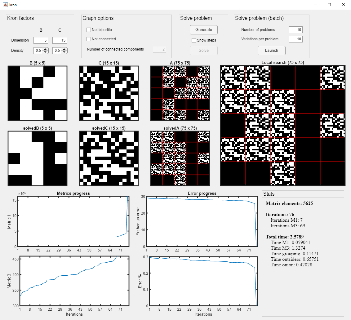
Figure 6: Kronecker factorization application.. A sample snapshot of the MATLAB application implementing the heuristic.

We implemented the heuristic described in Section 5 in the MATLAB programming environment; the source code is available online at https://github.com/calderonil/kron. The program provides a graphical user interface (Figure 6) that allows the user to generate a random binary matrix $\mathbf{A}$ of given size $\mathit{dimA}=\mathit{dimB}\times\mathit{dimC}$; the program then looks for a permutation $\mathbf{P}$ such that $\mathbf{A}=\mathbf{P}^{\intercal}(\mathbf{B}\operatorname{\otimes}\mathbf{C})\mathbf{P}$ where $\mathbf{B}$ and $\mathbf{C}$ are binary matrices of size $\mathit{dimB}\times\mathit{dimB}$ and $\mathit{dimC}\times\mathit{dimC}$, respectively. $\mathbf{A}$ is generated starting from random $\mathbf{P},\mathbf{B},\mathbf{C}$, which are then ”forgotten” and must therefore be computed from scratch; this ensures that a factorization of $\mathbf{A}$ always exists. The user must provide the densities $\rho_{B},\rho_{C}$ (fraction of 1s) of matrices $\mathbf{B},\mathbf{C}$; the density $\rho_{A}$ of $\mathbf{A}$ will therefore be $\rho_{A}=\rho_{B}\times\rho_{C}$. Although our application allows the user to impose additional constraints on the graph represented by the matrices (e.g., non-bipartitedness and/or non-connectedness), we did not impose any constraint for the experiments described in this section.

$\boldsymbol{\rho_{B},\rho_{C},\rho_{A}}$	Size of $B$	$\boldsymbol{\alpha}$	Size of $C$	Size of $A$	failure %	$\boldsymbol{t_{min}}$	$\boldsymbol{t_{avg}^{\prime}}$	$\boldsymbol{t_{avg}}$	$\boldsymbol{t_{max}}$
$0.5$, $0.5$, $0.25$	$5\times 5$	$1$	$5\times 5$	$25\times 25$	$0.00\%$	$0.02$	$0.03$	$0.06$	$0.31$
		$2$	$10\times 10$	$50\times 50$	$0.00\%$	$0.07$	$0.09$	$0.13$	$0.82$
		$3$	$15\times 15$	$75\times 75$	$0.00\%$	$0.18$	$0.21$	$0.27$	$0.81$
	$7\times 7$	$1$	$7\times 7$	$49\times 49$	$0.00\%$	$0.08$	$0.11$	$0.24$	$1.28$
		$2$	$14\times 14$	$98\times 98$	$0.00\%$	$0.35$	$0.43$	$0.67$	$2.55$
		$3$	$21\times 21$	$147\times 147$	$1.00\%$	$1.00$	$1.30$	$2.85$	$35.72$
	$10\times 10$	$1$	$10\times 10$	$100\times 100$	$0.00\%$	$0.52$	$0.59$	$1.42$	$11.59$
		$2$	$20\times 20$	$200\times 200$	$0.00\%$	$2.50$	$2.77$	$3.49$	$16.57$
		$3$	$30\times 30$	$300\times 300$	$0.00\%$	$6.71$	$7.54$	$8.47$	$10.89$
$0.6$, $0.6$, $0.36$	$5\times 5$	$1$	$5\times 5$	$25\times 25$	$0.00\%$	$0.01$	$0.03$	$0.06$	$0.52$
		$2$	$10\times 10$	$50\times 50$	$0.00\%$	$0.06$	$0.08$	$0.24$	$3.14$
		$3$	$15\times 15$	$75\times 75$	$0.00\%$	$0.16$	$0.19$	$0.27$	$1.41$
	$7\times 7$	$1$	$7\times 7$	$49\times 49$	$0.00\%$	$0.07$	$0.12$	$0.45$	$2.33$
		$2$	$14\times 14$	$98\times 98$	$3.00\%$	$0.39$	$0.45$	$1.20$	$15.30$
		$3$	$21\times 21$	$147\times 147$	$0.00\%$	$0.90$	$1.05$	$1.80$	$35.97$
	$10\times 10$	$1$	$10\times 10$	$100\times 100$	$0.00\%$	$0.36$	$0.51$	$0.85$	$8.42$
		$2$	$20\times 20$	$200\times 200$	$0.00\%$	$2.14$	$2.67$	$7.14$	$87.05$
		$3$	$30\times 30$	$300\times 300$	$0.00\%$	$6.58$	$7.98$	$16.79$	$210.95$
$0.7$, $0.7$, $0.49$	$5\times 5$	$1$	$5\times 5$	$25\times 25$	$1.00\%$	$0.01$	$0.04$	$0.09$	$1.06$
		$2$	$10\times 10$	$50\times 50$	$1.00\%$	$0.07$	$0.17$	$0.63$	$6.22$
		$3$	$15\times 15$	$75\times 75$	$4.00\%$	$0.14$	$0.34$	$0.84$	$10.32$
	$7\times 7$	$1$	$7\times 7$	$49\times 49$	$0.00\%$	$0.06$	$0.18$	$0.50$	$3.21$
		$2$	$14\times 14$	$98\times 98$	$7.00\%$	$0.32$	$1.18$	$1.97$	$18.71$
		$3$	$21\times 21$	$147\times 147$	$9.00\%$	$0.88$	$6.21$	$8.56$	$102.26$
	$10\times 10$	$1$	$10\times 10$	$100\times 100$	$0.00\%$	$0.25$	$0.45$	$1.84$	$19.42$
		$2$	$20\times 20$	$200\times 200$	$9.00\%$	$2.16$	$5.84$	$14.91$	$128.62$
		$3$	$30\times 30$	$300\times 300$	$0.00\%$	$5.84$	$6.65$	$19.91$	$243.12$

Table 2: Each row summarizes the performance of our heuristic on $10$ different initial random matrices $\mathbf{A}$; for each matrix $\mathbf{A}$ we executed the heuristic $10$ times, each one starting from a random permutation of $\mathbf{A}$. $\alpha=\mathit{dimC}/\mathit{dimB}$ is the ratio between the sizes of $\mathbf{C}$ and $\mathbf{B}$. $t_{avg}^{\prime}$ is the average of the minimum execution times of each different problem. The time spent on instances for which no solution has been found have been excluded from average, minimum and maximum execution times.

The combinations of parameters used in the experiments are shown in Table 2. The density (fraction of 1s) of $\mathbf{A},\mathbf{B},\mathbf{C}$ are denoted as $\rho_{A}$, $\rho_{B}$ and $\rho_{C}$, respectively. We consider several combinations of sizes $\mathit{dimB},\mathit{dimC}$ according to a parameter $\alpha$ that denotes the ratio between the size of $\mathbf{C}$ and $\mathbf{B}$ ($\alpha=\mathit{dimC}/\mathit{dimB}$). Intuitively, high values of $\alpha$ denotes that the size of the factors of $\mathbf{A}$ are different.

Each row of the table summarizes the result of one run: a run consists of $10$ random problem instances with the chosen parameters. Since our heuristic is sensitive to the initial conditions, for each instance we consider $10$ initial random permutation of the matrix $\mathbf{A}$; this is equivalent of fixing $\mathbf{B},\mathbf{C}$ and choosing ten different random permutation matrices $\mathbf{P}$. Therefore, each row summarizes $10\times 10$ executions of our program.

The program has been executed on a desktop PC with an Intel Xeon CPU running at $3.30$ GHz with $16$ GB of RAM running Windows 10 (Matlab R2021a). Both a single instance mode and a batch mode are provided; the former solves a single problem, while the latter generates a set of random instances with the same parameters ($\mathit{dimA},\mathit{dimB},\mathit{dimC}$). To collect the results we show in the following, the program was executed in batch mode.

For a single instance, our program executes alternateLocalSearch for at most $500$ iterations (see them main loop of Algorithm 2 in the Appendix); when no feasible factorization is found after the maximum allowed number of iterations, the procedure stops and the failure count is incremented.

For each run we collect five metrics: the percentage of executions at the end of which no factorization was found (failure %); the minimum and maximum execution times in seconds ($t_{min}$ and $t_{max}$, respectively); the average execution time across all executions that did find the optimal solution ($t_{avg}$); the average of the minimum execution time for each different problem ($t_{avg}^{\prime}$). More precisely, $t_{\mathit{min}}^{\prime}$ is computed as follows:

1. For each combination of parameters, we generate $10$ random instances consisting of matrices $\mathbf{A},\mathbf{B},\mathbf{C}$ of the appropriate size and content;

2. For each instance, we generate $10$ random permutation matrices $\mathbf{P}$; we get $10$ variations $\mathbf{A}=\mathbf{P}^{\intercal}(\mathbf{B}\operatorname{\otimes}\mathbf{C})\mathbf{P}$ that only differ by the permutation $\mathbf{P}$

3. We compute the minimum time to get the solution of the $10$ variations from the previous step;

4. $t_{\mathit{ave}}^{\prime}$ is the average of the minimum times computed at the previous step.

$t_{\mathit{avg}}^{\prime}$ is useful because there is a significant variance across the execution times of the $10$ variations of the same problem (see below). Indeed, as stated above, there might be a huge variation in the time required to factorize a matrix $\mathbf{A}=\mathbf{P}^{\intercal}(\mathbf{B}\operatorname{\otimes}\mathbf{C})\mathbf{P}$ depending on the permutation $\mathbf{P}$. Therefore, $t_{avg}^{\prime}$ is the average time to solve a problem instance if we were able to parallelize the heuristic across $10$ independent execution units, so that the first one that gets the solution stops the computation.

Figure 7: Dependence of the execution time on the number of 1s of $\mathbf{A}$.. Given $\rho_{A}=0.25$ and $dimB=10$, this chart shows the linear growth for $t_{avg}$ and $t_{avg}^{\prime}$ depending on the size of $\mathbf{C}$. Showing the matrix dimension in the $x$-axis could be misleading, the number of edges in $\mathbf{A}$ is used instead.

As can be observed from Table 2, the minimum time to compute a solution is very low (a few seconds) for all problems. The largest matrix $\mathbf{A}$ (size $300\times 300$) can be factored in $t_{min}=6.71s$. It should be observed that as the density of $\mathbf{A}$ increases, the problem becomes more difficult for our heuristic as witnessed by the increasing fraction of unsolved instances. We also observe that there is a large variability between the minimum and maximum times required to solve an instance; indeed we observe that the gap between $t_{\mathit{min}}$ and $t_{\mathit{max}}$ becomes more than an order of magnitude, especially for large matrices $\mathbf{A}$ that are decomposed into factors of unbalanced sizes ($\alpha=3$). This is due to the fact that the heuristic is sensitive to both the permutation $\mathbf{P}$, and to the sequence of swaps that are applied during the computation (the swaps are in part generated pseudo-randomly).

We not turn our attention to the study of the dependence of the execution time on the number of edges of the graph whose adjacency matrix is $\mathbf{A}$; the number of edges is simply the number of 1s in $\mathbf{A}$. To this aim, we performed $60$ additional experiments ($6$ separate problem instances with $10$ initial random permutation each). We set $\rho_{A}=0.25$ and $dimB=10$, and we increased the dimension of $\mathbf{C}$ with a step of $50$. Figure 7 shows the mean execution time $t_{\mathit{avg}}$ and As shown in Figure 7, $t_{avg}$ and $t_{avg}^{\prime}$ seems to grow more or less linearly with respect to the number of edges of $\mathbf{A}$.

7 Conclusions and future works

In this paper we presented a heuristic for decomposing a directed graph into factors according to the direct product: given a directed, unweighted graph $G$ with adjacency matrix $\mathbf{Adj(\mathnormal{G})}$, our heuristic searches for a pair of graphs $G_{1}$ and $G_{2}$ such that $G=G_{1}\operatorname{\times}G_{2}$, where $G_{1}\operatorname{\times}G_{2}$ is the direct product of $G_{1}$ and $G_{2}$. The heuristic proposed in this paper represents – to the best of our knowledge – the first computational approach for general directed, unweighted graphs. We provided a MATLAB implementation that we used to run a set of computational experiments to assess the effectiveness of our approach. Our implementation can factorize a graph of size $300\times 300$ in a few seconds. In a few worst-case scenarios the time grows to a few minutes, and is due to the fact that our heuristic is sensitive to the structure of the input; although it may fail to find a solution, in our experiments we observed failures in just a few instances.

We are planning to extend the heuristic along two directions: first, to handle weighted graphs instead of just unweighted ones; second, to compute the approximate Kronecker decomposition of unweighted graphs, where (a suitable permutation of) the input matrix $\mathbf{A}$ can be expressed as a Kronecker product of two smaller matrices $\mathbf{B}$ and $\mathbf{C}$, plus an additional binary error term $\mathbf{E}$, i.e., $\mathbf{A}=\mathbf{P}^{\intercal}(\mathbf{B}\operatorname{\otimes}\mathbf{C})\mathbf{P}+\mathbf{E}$.

Pseudocode

We provide here a more accurate description of our heuristic by means of pseudocode. The complete source code of the Matlab implementation can be downloaded from https://github.com/calderonil/kron.

Input: A, dimB, dimC

Output: solvedA, solvedB, solvedC

bestA = A;

metric = var;

A = kronGrouping(A);

/* Main loop */

while iter $\leq$ maxiter do

       iter++;

       if $\sim$blockMatrix then

            bestSwaps = outsiders(bestA);

       end if

      

      if $\sim$cornerizedMatrix $\wedge$ blockMatrix then

             if $\sim$balancedBlocks then

                   /* Blocks have a different number of 1s, unfeasible factorization */

                   bestA = randPerm(bestA,75%);

                   bestA = kronGrouping(bestA);

                   blockMatrix = false;

                  

             end if

            

       end if

      

      if $\sim$cornerizedMatrix $\wedge$ blockMatrix then

             [bestA, success] = onionSearch(bestA);

             if success then

                  break;

            else

                  continue;

             end if

            

       end if

      

      swaps = [bestSwaps,baseSwaps];

        // baseSwaps: all comb. of {1…dimA} two at a time

      

      for i=1 to len(swaps) do

             if bestSwaps exhausted then

                   baseSwaps = randPerm(baseSwaps,100%);

                   if metric == frob then

                         bestA = randPerm(bestA,45%);

                         bestA = kronGrouping(bestA);

                         blockMatrix = false;

                         cornerizedMatrix = false;

                        

                   end if

                  if metric == var then

                        metric = frob;

                   end if

                  

             end if

            

            curSwap = swaps(i);

             testA = swap(bestA, curSwap);

            

            if improved then

                   bestA = testA;

                   if metric == var $\wedge$ curVal $\geq$ threshold then

                        metric = frob

                   end if

                  break;

             end if

            

       end for

      

      [solvedB, solvedC] = nearestKronProduct(bestA);

      

      if $\sim$improved then

             nRestarts++;

             if nRestarts $\bmod$ perturbateEvery == 0  then

                   bestA = randPerm(bestA,100%);

                   bestA = kronGrouping(bestA);

                   blockMatrix = false;

                   cornerizedMatrix = false;

                   metric = var;

                  

            else

                   swapMetric();

                  

             end if

            

       end if

      

      if nRestarts $>$ maxRestarts $*$ perturbateEvery $\vee$ error $<0.000001$ then

            break;

            

       end if

      

end while

return bestA, solvedB, solvedC;

Algorithm 2 Alternate local search

Input: A

Output: groupedA

for i=1 to dimA do

       for j=1 to dimA do

             if i==j then

                  MR(i,j)=MC(i,j)=0;

            else

                   /* Simil computes the similarity between two rows/cols relying on the dot product. To weight zero-based and one-based similarity, both A and 1-A are considered. */

                   MR(i,j) = simil(A(i,:),A(j,:)) + simil(1-A(i,:),1-A(j,:));

                   MC(i,j) = simil(A(:,i),A(:,j)) + simil(1-A(:,i),1-A(:,j));

                  

             end if

            

       end for

      

end for

/* Six different permutations are tested, each one relying on a linear combination of rows similarity and columns similarity. */

for w=0 to 1 step 0.2 do

       MS = w * MR + (1-w) * MC;

       for i=1 to dimA do

             pivot = first unused index;

             scan MS(pivot,:) for the (dimC-1) best indexes and add them to the current permutation;

            

       end for

      

end for

return best permutation according to metric = frob

Algorithm 3 Kron grouping

Comment to Algorithm 4

At the beginning, outsiders identifies which block of $\mathbf{A}$ should receive 1s (because it already has more 1s than average) and which block should lose 1s. Then, two matrices are produced, $\mathbf{WR}$ and $\mathbf{WC}$. $\mathbf{WR}$ contains the number of 1s found in each portion of a row of length $dimC$ — the portion of the row corresponding to a given block. If the block should receive 1s, the number of zeros is counted instead. The second matrix $\mathbf{WC}$ contains the same information computed column-wise. A third matrix $\mathbf{MS}$ is computed in order to find the best swap: the procedure loops on each row/column on a block-by-block basis and multiplies the elements of $\mathbf{WR}$ and $\mathbf{WC}$ corresponding to blocks that are in opposite conditions, i.e. one receives and the other loses 1s. The larger the values of $\mathbf{MW}$, the better. This product is tuned according to the density of the block that receives 1s. However, moving elements in blocks that already have a high number of 1s would produce blocks with too many 1s, which are unlikely to appear in a feasible factorization. Elements of $\mathbf{MS}$ are scanned and ordered to form the list of more promising swaps. If $\mathbf{MS}$ has zero elements only, there are no 1s on the blocks that should lose 1s. Therefore, according to Definition 4, the matrix is a block matrix.

Input: A

Output: bestSwaps

BL = blockMatrix(A);

  // derive the dimB x dimB block matrix

S = blocksSum(BL);

  // count the total number of 1s in each block

D = blocksDensity(BL);

  // computes the density of 1s in each block

foreach B in BL do

       for k=1 to dimC do

             sumRow = sum(B(k,:));

             sumCol = sum(B(:,k));

             if S(B) $<$ avg(S) then

                   /* The block is likely to be emptied, count the number of 1s */

                   WR(((row(B)-1)*dimC)+k,col(B)) = sumRow;

                   WC(row(B),((col(B)-1)*app.dimC)+k) = sumCol;

                  

            else

                   /* The block is likely to be filled, count the number of zeros */

                   WR(((row(B)-1)*dimC)+k,col(B)) = -(dimC-sumRow);

                   WC(row(B),((col(B)-1)*app.dimC)+k) = -(dimC-sumCol);

                  

             end if

            

       end for

      

end foreach

for i=1 to dimA do

       p = blockIdx(i);

       for j=1 to dimA do

             q = blockIdx(j);

             if i and j fall in different blocks then

                   for b=1 to dimB do

                         if BL(p,b) is a block to be emptied and BL(q,b) a block to be filled then

                               MS(i,j) = MS(i,j) + (WR(i,b) * WR(j,b) * (1-D(q,b))²);

                              

                         end if

                        if BL(p,b) is a block to be filled and BL(q,b) a block to be emptied then

                               MS(i,j) = MS(i,j) + (WR(i,b) * WR(j,b) * (1-D(p,b))²);

                              

                         end if

                        if BL(b,p) is a block to be emptied and BL(b,q) a block to be filled then

                               MS(i,j) = MS(i,j) + (WC(b,i) * WC(b,j) * (1-D(b,q))²);

                              

                         end if

                        if BL(b,p) is a block to be filled and BL(b,q) a block to be emptied then

                               MS(i,j) = MS(i,j) + (WC(b,i) * WC(b,j) * (1-D(b,p))²);

                              

                         end if

                        

                   end for

                  

             end if

            

       end for

      

end for

if sum(MS)==0 then

       blockMatrix = true;

       return null;

      

else

       return a list of swaps (i,j) in ascending order of MS(i,j);

      

end if

Algorithm 4 Outsiders

Input: A

Output: A

/* ------- PART1: rearrange the filled blocks in a top-left fashion --------- */

BL = blockMatrix(A);

EF = checkFilledBlocks(BL);

  // derive a boolean block matrix; 0: empty block, 1: o.w.

W = weightMatrix(dimB);

  // the max weight corresponds to the top-left block

cornerizeVal = sum(dotProduct(EF,W));

for iter = 1 to maxiterCornerize do

       for i=1 to len(swaps) do

             curSwap = swaps(i);

             testEF = swap(EF, curSwap);

             testVal = sum(dotProduct(testEF,W));

            

            if testVal $>$ cornerizeVal then

                   cornerizeVal = testVal;

                   EF = testEF;

                   BL = swap(BL, curSwap);

                   break;

             end if

            

       end for

      

      if cornerizeVal $>$ 0.75 * cornerizeOptVal then

             break;

       end if

      if $\sim$improved then

             BL = randPerm(BL,55%);

             Apply the same permutation to EF;

            

       end if

      

end for

cornerizedMatrix = true;

/* ----- PART2: perform a layer-by-layer Kron factorization on submatrices -- */

A = fromBlocks(BL);

settledLayers = 1;

for curlayer = 2 to dimB do

       /* In localSearchSubmatrix swaps are limited to the range of blocks [settledLayers+1, curLayer]. Moreover, only the Frobenius metric is used. */

       [success, A] = localSearchSubmatrix(A, curLayer, settledLayers);

       if success then

             settledLayers = curLayer;

            

       end if

      

end for

return success, A;

Algorithm 5 Onion search

Comment to Algorithm 5

The procedure onionSearch is divided in two parts. First, the block matrix is rearranged to push the maximum feasible number of blocks to the top-left corner to facilitate the second step. A binary block matrix $\mathbf{EF}$ is derived from $\mathbf{A}$ and it is permuted to maximize the dot product with the weight matrix $\mathbf{W}$. To find a convenient permutation, random swaps are applied following the same principle of the main local search. When the procedure reaches the $75\%$ of the optimum, the block matrix is deemed to be sufficiently rearranged in a top-left fashion and the procedure terminates. The second part of onionSearch tries to find a feasible factorization for submatrices following a layer-by-layer perspective. The local search follows the same principles of alternateLocalSearch but uses metric frob only through the subroutine localSearchSubmatrix. It is important to note that the single block $\mathbf{B}_{11}$ representing the first layer is implicitly factorized as $\mathbf{B}_{11}=\mathbf{I}_{1}\operatorname{\otimes}\mathbf{B}_{11}$. It is thus used as template during the local search performed on the successive $2\times 2$ blocks submatrix, composed of four blocks. The procedure steps forward until the last layer is processed. If the local search on the last layer succeeds, the problem is globally solved. Otherwise, alternateLocalSearch proceeds testing swaps randomly to find a feasible solution.

References

- Arndt [2004] H. Arndt. Load balancing: dimension exchange on product graphs. In 18th International Parallel and Distributed Processing Symposium, 2004. Proceedings., pages 20–, 2004. doi: 10.1109/IPDPS.2004.1302928.
- Calderoni et al. [2021] Luca Calderoni, Luciano Margara, and Moreno Marzolla. Direct product primality testing of graphs is gi-hard. Theoretical Computer Science, 860:72–83, 2021. ISSN 0304-3975. doi: 10.1016/j.tcs.2021.01.029.
- Diekert and Kausch [2016] Volker Diekert and Jonathan Kausch. Logspace computations in graph products. Journal of Symbolic Computation, 75:94–109, 2016. ISSN 0747-7171. doi: https://doi.org/10.1016/j.jsc.2015.11.009. URL https://www.sciencedirect.com/science/article/pii/S074771711500108X. Special issue on the conference ISSAC 2014: Symbolic computation and computer algebra.
- Hammack et al. [2011] Richard Hammack, Wilfried Imrich, and Sandi Klavžar. Handbook of Product Graphs, Second Edition. Discrete Mathematics and Its Applications. Taylor & Francis, 2011. ISBN 9781439813041.
- Imrich [1998] Wilfried Imrich. Factoring cardinal product graphs in polynomial time. Discrete Mathematics, 192(1):119–144, 1998. ISSN 0012-365X. doi: 10.1016/S0012-365X(98)00069-7.
- Jooya et al. [2016] Hossein Z. Jooya, Kamran Reihani, and Shih-I Chu. A graph-theoretical representation of multiphoton resonance processes in superconducting quantum circuits. Scientific Reports, 6, 2016. doi: 10.1038/srep37544.
- Leskovec et al. [2010] Jure Leskovec, Deepayan Chakrabarti, Jon Kleinberg, Christos Faloutsos, and Zoubin Ghahramani. Kronecker graphs: An approach to modeling networks. J. Mach. Learn. Res., 11:985–1042, March 2010. ISSN 1532-4435.
- Loan [2000] Charles F.Van Loan. The ubiquitous Kronecker product. Journal of Computational and Applied Mathematics, 123(1):85–100, 2000. ISSN 0377-0427. doi: 10.1016/S0377-0427(00)00393-9. Numerical Analysis 2000. Vol. III: Linear Algebra.
- Van Loan and Pitsianis [1993] C. F. Van Loan and N. Pitsianis. Approximation with Kronecker products. In Marc S. Moonen, Gene H. Golub, and Bart L. R. De Moor, editors, Linear Algebra for Large Scale and Real-Time Applications, pages 293–314. Springer Netherlands, Dordrecht, 1993. ISBN 978-94-015-8196-7. doi: 10.1007/978-94-015-8196-7˙17.
- Weichsel [1962] Paul M. Weichsel. The kronecker product of graphs. Proceedings of the American Mathematical Society, 13(1):47–52, 1962.