A stochastic first-order trust-region method with inexact restoration for finite-sum minimization

Abstract

We propose a stochastic first-order trust-region method with inexact function and gradient evaluations for solving finite-sum minimization problems. Using a suitable reformulation of the given problem, our method combines the inexact restoration approach for constrained optimization with the trust-region procedure and random models. Differently from other recent stochastic trust-region schemes, our proposed algorithm improves feasibility and optimality in a modular way. We provide the expected number of iterations for reaching a near-stationary point by imposing some probability accuracy requirements on random functions and gradients which are, in general, less stringent than the corresponding ones in literature. We validate the proposed algorithm on some nonconvex optimization problems arising in binary classification and regression, showing that it performs well in terms of cost and accuracy, and allows to reduce the burdensome tuning of the hyper-parameters involved.

Keywords: finite-sum minimization, inexact restoration, trust-region methods, subsampling, worst-case iteration complexity.

1 Introduction

In this paper we consider the finite-sum minimization problem

$$\min_{x\in\hbox{\rm I\kern-1.39998pt\hbox{\rm R}}^{n}}f_{N}(x)=\frac{1}{N}\sum_{i=1}^{N}\phi_{i}(x),$$ (1)

where $N$ is very large and finite and $\phi_{i}:\hbox{\rm I\kern-1.99997pt\hbox{\rm R}}^{n}\rightarrow\hbox{\rm I\kern-1.99997pt\hbox{\rm R}}$, $1\leq i\leq N$, are continuously differentiable. A number of important problems can be stated in this form, e.g., classification problems in machine learning, data fitting problems, sample average approximations of an objective function given in the form of mathematical expectation. In recent years the need for efficient methods for solving (1) resulted in a large body of literature and a number of methods have been proposed and analyzed, see e.g., the reviews [3, 21, 12].

It is common to employ subsampled approximations of the objective function and its derivatives with the aim of reducing the computational cost. Focusing on first-order methods, the stochastic gradient [33] and more contemporary variants like SVRG [24, 25], SAG [34], ADAM [26] and SARAH [31] are widely used for their simplicity and low cost per-iteration. They do not call for function evaluations but require tuning the learning rate and further possible hyper-parameters such as the mini-batch size. Since the tuning effort may be very computationally demanding [19], more sophisticated approaches use stochastic linesearch or trust-region strategies to adaptively choose the learning rate, see [5, 3, 7, 11, 18, 19, 32]. In this context, function and gradient approximations have to satisfy sufficient accuracy requirements with some probability. This, in turn, in case of approximations via sampling, requires adaptive choices of the sample sizes used.

In a further stream of works, problem (1) is reformulated as a constrained optimization problem and the sample size is computed deterministically using the Inexact Restoration (IR) approach. The IR approach has been successfully combined with either the linesearch strategy [27] or the trust-region strategy [9, 10, 4]; in these papers, function and gradient estimates are built with gradually increasing accuracy and averaging on the same sample.

We propose a novel trust-region method with random models based on the IR methodology. In our proposed method, feasibility and optimality are improved in a modular way, and the resulting procedure differs from the existing stochastic trust-region schemes [1, 11, 6, 18, 35] in the acceptance rule for the step. We provide a theoretical analysis and give a bound on the expected iteration complexity to satisfy an approximate first-order optimality condition; this calls for accuracy conditions on random gradients that are assumed to hold with some sufficiently large but fixed probability and are, in general, less stringent than the corresponding ones in [1, 11, 6, 18, 35]. Our theoretical analysis improves over the one for the stochastic trust-region method with inexact restoration given in [4], since we no longer rely on standard theory for deterministic unconstrained optimization invoked eventually when functions and gradients are computed exactly.

The paper is organized as follows. In Section 2 we give an overview of random models employed in the trust-region framework and introduce the main features of our contribution. The new algorithm is proposed in Section 3 and studied theoretically with respect to the iteration complexity analysis. Extensive numerical results are presented in Section 4.

2 Trust-region method with random models

Variants of the standard trust-region method based on the use of random models have been presented, to our knowledge, in [4, 1, 6, 11, 18, 17, 35]. They consist in the adaptation of the trust-region framework to the case where random estimates of the derivatives are introduced and function values are either computed exactly [1] or replaced by stochastic estimates [4, 11, 6, 18, 17, 35].

The computation and acceptance of the iterates parallel the standard trust-region mechanism, and the success of the procedure relies on function values and models being sufficiently accurate with fixed and large enough probability. The accuracy requests in the mentioned works show many similarities; here we illustrate some issues related to the works [11, 18, 35], which are closer to our approach.

Let $\|\cdot\|$ denote the 2-norm throughout the paper. At iteration $k$ of a first-order stochastic trust-region model, given $x_{k}$, the positive trust-region radius $\delta_{k}$ and a random approximation $g_{k}$ of $\nabla f_{N}(x_{k})$, let consider the model

$$\varsigma_{k}(x_{k}+s)=f_{N}(x_{k})+g_{k}^{T}s$$

for $f_{N}$ on $B(x_{k},\delta_{k})=\{x\in\mathbb{R}^{n}:\|x-x_{k}\|\leq\delta_{k}\}$ and the trust-region problem $\min_{\|s\|\leq\delta_{k}}\varsigma_{k}(x_{k}+s)$. Thus, the trust region step takes the form $s_{k}=-\delta_{k}g_{k}/\|g_{k}\|$.

Two estimates $f^{k,0}$ and $f^{k,s}$ of $f_{N}$ at $x_{k}$ and $x_{k}+s_{k}$, respectively, are employed to either accept or reject the trial point $x_{k}+s_{k}$. The classical ratio between the actual and predicted reduction is replaced by

$$\rho_{k}=\displaystyle\frac{f^{k,0}-f^{k,s}}{\varsigma_{k}(x_{k})-\varsigma_{k}(x_{k}+s_{k})},$$ (2)

and a successful iteration is declared when $\rho_{k}\geq\eta_{1}$ and $\|g_{k}\|\geq\eta_{2}\delta_{k}$ for some constants $\eta_{1}\in(0,1)$ and positive and possibly large $\eta_{2}$. Note that the computation of both the step $s_{k}$ and the denominator in (2) are independent of $f_{N}(x_{k})$. Furthermore, note that a successful iteration might not yield an actual reduction in $f_{N}$ because the quantities involved in $\rho_{k}$ are random approximations to the true value of the objective function.

The condition $\|g_{k}\|\geq\eta_{2}\delta_{k}$ is not typical of standard trust-region and depends on the fact that $\delta_{k}$ controls the accuracy of function and gradients. Specifically, the models used are required to be sufficiently accurate with some probability. The model $\varsigma_{k}$ is supposed to be, $p_{M}$-probabilistically, a $\kappa_{*}$-fully linear model of $f_{N}$ on the ball $B(x_{k},\delta_{k})$, i.e., the requirement

$$|f_{N}(y)-\varsigma_{k}(y)|\leq\kappa_{*}\delta_{k}^{2},\quad\|\nabla f_{N}(y)-g_{k}\|\leq\kappa_{*}\delta_{k},\quad y\in B(x_{k},\delta_{k})$$ (3)

with $\kappa_{*}>0$, has to be fulfilled at least with probability $p_{M}\in(0,1)$. Moreover, the estimates $f^{k,0}$ and $f^{k,s}$ are supposed to be $p_{f}$-probabilistically $\epsilon_{F}$-accurate estimates of $f_{N}(x_{k})$ and $f_{N}(x_{k}+s_{k})$, i.e., the requirement

$$|f^{k,0}-f_{N}(x_{k})|\leq\epsilon_{F}\delta_{k}^{2},\quad|f^{k,s}-f_{N}(x_{k}+s_{k})|\leq\epsilon_{F}\delta_{k}^{2},$$ (4)

has to be fulfilled at least with probability $p_{f}\in(0,1)$. Clearly, if $f_{N}$ is computed exactly then condition (4) is trivially satisfied.

Convergence analysis in [11, 18, 35] shows that for $p_{M}$ and $p_{f}$ sufficiently large it holds $\lim_{k\rightarrow\infty}\delta_{k}=0$ almost surely. Moreover, if $f_{N}$ is bounded from below and $\nabla f_{N}$ is Lipschitz continuous, then $\lim_{k\rightarrow\infty}\|\nabla f_{N}(x_{k})\|=0$ almost surely. Interestingly, the accuracy in (3) and (4) increases as the trust region radius gets smaller but the probabilities $p_{M}$ and $p_{f}$ are fixed.

For problem (1) it is straightforward to build approximations of $f_{N}$ and $\nabla f_{N}$ by sample average approximations

$$f_{M}(x)=\frac{1}{M}\sum_{i\in I_{M}}\phi_{i}(x),\qquad\nabla f_{S}(x)=\frac{1}{S}\sum_{i\in I_{S}}\nabla\phi_{i}(x),$$ (5)

where $I_{M}$ and $I_{S}$ are subsets of $\{1,\ldots,N\}$ of cardinality $|I_{M}|=M$ and $|I_{S}|=S$, respectively. The choice of sample size such that (3) and (4) hold in probability is discussed in [18, §5] as follows. Let $\mathbb{E}[|\phi_{i}(x)-f_{N}(x)|^{2}]\leq V_{f}$, $\mathbb{E}[|\nabla\phi_{i}(x)-\nabla f_{N}(x)|^{2}]\leq V_{g}$, $i=1,\ldots,N$, with $\mathbb{E}$ being the expected value of a random variable, and assume

$$M\geq\frac{V_{f}}{\epsilon_{F}^{2}(1-p_{f})\delta_{k}^{4}},\;\;\;\;\;S\geq\frac{V_{g}}{\kappa_{*}^{2}(1-p_{g})\delta_{k}^{2}}\\ \mbox{ and }\max\{M,S\}\leq N.$$ (6)

Then $f^{k,0}$ and $f^{k,s}$ built as in (5) with sample size $M$ satisfy (4) with probability $p_{f}$, while $g_{k}$ built as in (5) with sample size $S$ satisfies $\|\nabla f_{N}(x_{k})-g_{k}\|\leq\kappa_{*}\delta_{k}$ with probability $p_{g}$. Furthermore, using Taylor expansion and Lipschitz continuity of $\nabla f_{N}$, it can be proved that (3) is met with probability $p_{M}=p_{f}p_{g}$; consequently, a $\kappa_{*}$-fully linear model of $f_{N}$ in $B(x_{k},\delta_{k})$ is obtained.

In principle, conditions (3), (4) and $\lim_{k\rightarrow\infty}\delta_{k}=0$ imply that $f^{k,0}$, $f^{k,s}$ and $g_{k}$ will be computed at full precision for $k$ sufficiently large. On the other hand, in applications such as machine learning, reaching full precision is unlikely since $N$ is very large and termination is based on the maximum allowed computational effort or on the validation error.

2.1 Our contribution

We propose a trust-region procedure with random models based on (5) and combine it with the inexact restoration (IR) method for constrained optimization [30]. To this end, we make a simple transformation of (1) into a constrained problem. Specifically, letting $I_{M}$ be an arbitrary nonempty subset of $\{1,\ldots,N\}$ of cardinality $|I_{M}|$ equal to $M$, we reformulate problem (1) as

$$\min_{x\in\hbox{\rm I\kern-1.39998pt\hbox{\rm R}}^{n}}f_{M}(x)=\frac{1}{M}\sum_{i\in I_{M}}\phi_{i}(x),$$ (7)

$$\mbox{ s.t. }M=N.$$

Using the IR strategy allows to improve feasibility and optimality in a modular way and gives rise to a procedure that differs from the existing trust-region schemes in the following respects. First, at each iteration a reference sample size is fixed and used as a guess for the approximation of function values. Second, the acceptance rule for the step is based on the condition $\|g_{k}\|\geq\eta_{2}\delta_{k}$, for some $\eta_{2}>0$, and a sufficient decrease condition on a merit function that measures both the reduction of the objective function and the improvement in feasibility. Finally, the expected iteration complexity to satisfy an approximate first-order optimality condition is given, provided that, at each iteration $k$, the gradient estimates satisfy accuracy requirements of order ${\cal{O}}\left(\delta_{k}\right)$; such accuracy requirements implicitly govern function approximations and are, in general, less stringent than the corresponding ones in [1, 11, 6, 18, 35], as carefully detailed in Section 3.

Our theoretical analysis improves over the analysis carried out in [4] for a similar stochastic trust-region coupled with inexact restoration, since here we do not rely on the occurrence of full precision, $M=N$ in (7), reached eventually and do not apply standard theory for unconstrained optimization. In fact, the expected number of iterations until a prescribed accuracy is reached is provided without invoking full precision.

3 The Algorithm

In this section we introduce our new algorithm referred to as SIRTR (Stochastic Inexact Restoration Trust Region).

First, we introduce some issues of IR methods. The level of infeasibility with respect to the constraint $M=N$ in (7) is measured by the following function $h$.

Assumption 3.1.

Let $h:\{1,2,\ldots,N\}\rightarrow\hbox{\rm I\kern-1.99997pt\hbox{\rm R}}$ be a monotonically decreasing function such that $h(1)>0$, $h(N)=0$.

This assumption implies that there exist some positive $\underline{h}$ and $\overline{h}$ such that

$$\underline{h}\leq h(M)\ \ \mbox{ if }\ \ 1\leq M<N,\quad\mbox{ and }\quad h(M)\leq\overline{h}\ \ \mbox{ if }\ \ 1\leq M\leq N.$$ (8)

One possible choice is $h(M)=(N-M)/N,\ 1\leq M\leq N$.

The IR methods improve feasibility and optimality in modular way using a merit function to balance the progress. Since the reductions in the objective function and infeasibility might be achieved to a different degree, the IR method employs the merit function

$$\Psi(x,M,\theta)=\theta f_{M}(x)+(1-\theta)h(M),$$ (9)

with $\theta\in(0,1).$

Our SIRTR algorithm is a trust-region method that employs first-order random models. At a generic iteration $k$, we fix a trial sample size $N_{k+1}^{t}$ and build a linear model $m_{k}(p)$ around $x_{k}$ of the form

$$m_{k}(p)=f_{N_{k+1}^{t}}(x_{k})+g_{k}^{T}p,$$ (10)

where $g_{k}$ is a random estimator to $\nabla f_{N}(x_{k})$. Then, we consider the trust-region problem

$$\min_{\|p\|\leq\delta_{k}}m_{k}(p),$$ (11)

whose solution is

$$p_{k}=-\delta_{k}\frac{g_{k}}{\|g_{k}\|}.$$ (12)

As in standard trust-region methods, we distinguish between successful and unsuccessful iterations. However, we do not employ here the classical acceptance condition, but a more elaborate one that involves the merit function (9).

The proposed method is sketched in Algorithm 1 and its steps are now discussed. At a generic iteration $k$, we have at hand the outcome of the previous iteration: the iterate $x_{k}$, the sample sizes $N_{k}$ and $\widetilde{N}_{k}$, the penalty parameter $\theta_{k}$, the flag iflag. If iflag=succ the previous iteration was successful, i.e., $x_{k}=x_{k-1}+p_{k-1}$, if iflag=unsucc the previous iteration was unsuccessful, i.e., $x_{k}=x_{k-1}$.

The scheduling procedure for generating the trial sample size $N_{k+1}^{t}$ consists of Steps 1 and 2 of SIRTR. At Step 1, we determine a reference sample size $\widetilde{N}_{k+1}\leq N$. If iflag=succ, then the infeasibility measure $h$ is sufficiently decreased as stated in (20). If iflag=unsucc, $\widetilde{N}_{k+1}$ is left unchanged from the previous iteration, i.e., $\widetilde{N}_{k+1}=\widetilde{N}_{k}$. We remark that (20) trivially implies $\widetilde{N}_{k+1}=N$ if $N_{k}=N$ and that it holds at each iteration, even when it is not explicitly enforced at Step 1 (see forthcoming Lemma 1). In principle $\widetilde{N}_{k+1}$ could be the trial sample size but we aim at giving more freedom to the sample size selection process. Thus, at Step 2, we choose a trial sample size $N_{k+1}^{t}$ complying with condition (21). On the one hand, such a condition allows the choice $N_{k+1}^{t}<\widetilde{N}_{k+1}$ in order to reduce the computational effort; on the other hand, the choice $N_{k+1}^{t}\geq\widetilde{N}_{k+1}$ is also possible in order to satisfy specific accuracy requirements that will be specified later. When $N_{k+1}^{t}<\widetilde{N}_{k+1}$, condition (21) rules the largest possible distance between $N_{k+1}^{t}$ and $\widetilde{N}_{k+1}$ in terms of $\delta_{k}$; in case $N_{k+1}^{t}\geq\widetilde{N}_{k+1}$, (21) is trivially satisfied.

At Step 3 we form the linear random model (10) and compute its minimizer. Specifically, we fix the cardinality $N_{k+1,g}$ and choose the set of indices $I_{N_{k+1,g}}\subseteq\{1,\ldots,N\}$ of cardinality $N_{k+1,g}$. Then, we compute the estimator $g_{k}$ of $\nabla f_{N}(x_{k})$ as

$$g_{k}=\frac{1}{N_{k+1,g}}\sum_{i\in I_{N_{k+1,g}}}\nabla\phi_{i}(x_{k})$$ (13)

and the solution $p_{k}$ in (12) of the trust-region subproblem (11). Further, we compute $m_{k}(p_{k})$ where $m_{k}$ is defined in (10) and

$$f_{N_{k+1}^{t}}(x_{k})=\frac{1}{N_{k+1}^{t}}\sum_{i\in I_{N_{k+1}^{t}}}\phi_{i}(x_{k}),$$ (14)

with $I_{N_{k+1}^{t}}\subseteq\{1,\ldots,N\}$ being a set of cardinality $N_{k+1}^{t}$.

At Step 4 we compute the new penalty term $\theta_{k+1}.$ The computation relies on the predicted reduction defined as

$${\rm{Pred}}_{k}(\theta)=\theta(f_{N_{k}}(x_{k})-m_{k}(p_{k}))+(1-\theta)(h(N_{k})-h(\widetilde{N}_{k+1})),$$ (15)

where $\theta\in(0,1)$. This predicted reduction is a convex combination of the usual predicted reduction $f_{N_{k}}(x_{k})-m_{k}(p_{k})$ in trust-region methods, and the predicted reduction $h(N_{k})-h(\widetilde{N}_{k+1})$ in infeasibility obtained in Step 1. The new parameter $\theta_{k+1}$ is computed so that

$${\rm{Pred}}_{k}(\theta)\geq\eta_{1}(h(N_{k})-h(\widetilde{N}_{k+1})).$$ (16)

If (16) is satisfied at $\theta=\theta_{k}$ then $\theta_{k+1}=\theta_{k}$, otherwise $\theta_{k+1}$ is computed as the largest value for which the above inequality holds (see forthcoming Lemma 3).

Step 5 establishes if the iteration is successful or not. To this end, given a point $\hat{x}$ and $\theta\in(0,1)$, the actual reduction of $\Psi$ at the point $\hat{x}$ has the form

$${\rm{Ared}}_{k}(\hat{x},\theta) = \Psi(x_{k},N_{k},\theta)-\Psi(\hat{x},N_{k+1}^{t},\theta)$$ (17)

$$= \theta(f_{N_{k}}{(x_{k})}-f_{N_{k+1}^{t}}(\hat{x}))+(1-\theta)(h(N_{k})-h(N_{k+1}^{t})),\qquad$$

and the iteration is successful whenever the following two conditions are both satisfied

$${\rm{Ared}}_{k}(x_{k}+p_{k},\theta_{k+1}) \geq\eta_{1}{\rm{Pred}}_{k}(\theta_{k+1})$$ (18)

$$\|g_{k}\| \geq\eta_{2}\delta_{k}.$$ (19)

Otherwise the iteration is declared unsuccessful. If the iteration is successful, we accept the step and the trial sample size, set iflag=succ and possibly increase the trust-region radius through (23); the upper bound $\delta_{\max}$ on the trust region size is imposed in (23). In case of unsuccessful iterations, we reject both the step and the trial sample size, set iflag=unsucc and decrease the trust region size.

Concerning conditions (18) and (19), we observe that the former mimics the classical acceptance criterion of standard trust-region methods while the latter drives $\delta_{k}$ to zero as $\|g_{k}\|$ tends to zero.

Algorithm 3.1: The Stochastic IRTR algorithm
Given $x_{0}\in\hbox{\rm I\kern-1.99997pt\hbox{\rm R}}^{n}$, $N_{0}$ integer in $(0,N]$, $\theta_{0}\in(0,1)$, $0<\delta_{0}<\delta_{\max}$, $\gamma>1,\,r,\eta_{1},\in(0,1),\;\mu,\,\eta_{2}>0$. 0. Set $k=0$, iflag=succ. 1. If iflag=succ
      Find $\widetilde{N}_{k+1}$ such that $N_{k}\leq\widetilde{N}_{k+1}\leq N$ and $$h(\widetilde{N}_{k+1})\leq rh(N_{k}),$$ (20) 1. Else set $\widetilde{N}_{k+1}=\widetilde{N}_{k}$. 2. If $N_{k}=N$ set $N_{k+1}^{t}=N$ 1. Else find $N_{k+1}^{t}$ such that $\displaystyle h(N_{k+1}^{t})-h(\widetilde{N}_{k+1})$ $\displaystyle\leq$ $\displaystyle\mu\delta_{k}^{2}.$ (21) 3. Choose $N_{k+1,g}$, $I_{N_{k+1,g}}\subseteq\{1,\ldots,N\}$ s.t. $|I_{N_{k+1,g}}|=N_{k+1,g}$. 1. Compute $g_{k}$ as in (13), and set $$p_{k}=-\delta_{k}\frac{g_{k}}{\|g_{k}\|}.$$ 1. Compute $f_{N_{k+1}^{t}}(x_{k})$ as in (14), and $m_{k}(p_{k})=f_{N_{k+1}^{t}}(x_{k})+g_{k}^{T}p_{k}$. 4. Compute the penalty parameter $\theta_{k+1}$ $\displaystyle\theta_{k+1}=\left\{\begin{array}[]{ll}&\theta_{k}\hskip 30.0pt\mbox{ if }\ {\rm{Pred}}_{k}(\theta_{k})\geq\eta_{1}(h(N_{k})-h(\widetilde{N}_{k+1}))\\ &\displaystyle\frac{(1-\eta_{1})(h(N_{k})-h(\widetilde{N}_{k+1}))}{m_{k}(p_{k})-f_{N_{k}}(x_{k})+h(N_{k})-h(\widetilde{N}_{k+1})}\quad\mbox{otherwise}.\end{array}\right.$ (22) 5. If ${\rm{Ared}}_{k}(x_{k}+p_{k},\theta_{k+1})\geq\eta_{1}{\rm{Pred}}_{k}(\theta_{k+1})$ and $\|g_{k}\|\geq\eta_{2}\delta_{k}$ (successful iteration) define $\displaystyle x_{k+1}$ $\displaystyle=x_{k}+p_{k}$ $\displaystyle\delta_{k+1}$ $\displaystyle=\min\left\{\gamma\delta_{k},\delta_{\max}\right\}$ (23) set $N_{k+1}=N_{k+1}^{t}$, $k=k+1$, iflag=succ and go to Step 1. Else (unsuccessful iteration) define $\displaystyle x_{k+1}$ $\displaystyle=x_{k}$ $\displaystyle\delta_{k+1}$ $\displaystyle=\frac{\delta_{k}}{\gamma}$ (24) set $N_{k+1}=N_{k}$, $k=k+1$, iflag=unsucc and go to Step 1. Fig. 1:

We conclude the description of Algorithm 1 showing that condition (20) holds for all iterations, even when it is not explicitly enforced at Step 1.

Lemma 1.

Let Assumption 3.1 holds and $r\in(0,1)$ be the scalar in Algorithm 1. The sample sizes $\widetilde{N}_{k+1}\leq N$ and $N_{k}\leq N$ generated by Algorithm 1 satisfy

$$h(\widetilde{N}_{k+1})\leq rh(N_{k}),\quad\forall k\geq 0.$$ (25)

Proof. We observe that, by Assumption 3.1, (25) trivially holds whenever $N_{k}=\widetilde{N}_{k+1}=N$.

Otherwise, we proceed by induction. Indeed, the thesis trivially holds for $k=0$, as we set iflag=succ at the first iteration and enforce (25) at Step 1. Now consider a generic iteration $\bar{k}\geq 1$ and suppose that (25) holds for $\bar{k}-1$. If iteration $\bar{k}-1$ is successful, then condition (25) is enforced for iteration $\bar{k}$ at Step 1.

If iteration $\bar{k}-1$ is unsuccessful, then at Step 5 we set $N_{\bar{k}}=N_{\bar{k}-1}$. Successively, at Step 1 of iteration $\bar{k}$ we set $\widetilde{N}_{\bar{k}+1}=\widetilde{N}_{\bar{k}}$. Since (25) holds by induction at iteration $\bar{k}-1$, we have $h(\widetilde{N}_{\bar{k}})\leq rh(N_{\bar{k}-1})$, which can be rewritten as $h(\widetilde{N}_{\bar{k}+1})\leq rh(N_{\bar{k}})$ due to the previous assignments at Step 5 and Step 1. Then condition (25) holds also at iteration $\bar{k}$. $\Box$

3.1 On the sequences $\{\theta_{k}\}$ and $\{\delta_{k}\}$

In this section, we analyze the properties of Algorithm 1. In particular, we prove that the sequence $\{\theta_{k}\}$ is non increasing and uniformly bounded from below, and that the trust region radius $\delta_{k}$ tends to $0$ as $k\rightarrow\infty$. We make the following assumption.

Assumption 3.2.

Functions $\phi_{i}$ are continuously differentiable for $i=1,\ldots,n$. There exist $\Omega\subset\mathbb{R}^{n}$ and $f_{low}$, $f_{up}$ such that

$$f_{low}<f_{M}(x)<f_{up},\quad\ 1\leq M\leq N,\ x\in\Omega,$$

and all iterates generated by Algorithm 1 belong to $\Omega$.

In the following, we let

$$\kappa_{\phi}=\max\{|f_{low}|,|f_{up}|\}.$$ (26)

Remark 2.

In the context of machine learning, the above assumption is verified in several cases, e.g., the mean-squares loss function coupled with either the sigmoid, the softmax or the hyperbolic tangent activation function; the mean-squares loss function coupled with ReLU or ELU activation functions and proper bounds on the unknowns; the logistic loss function coupled with proper bounds on the unknowns [23].

In the analysis that follows we will consider two options for $\hat{x}$ in (17), $\hat{x}=x_{k}+p_{k}$ for successful iterations and $\hat{x}=x_{k}$ for unsuccessful iterations.

Our first result characterizes the sequence $\{\theta_{k}\}$ of the penalty parameters; the proof follows closely [4, Lemma 2.2].

Lemma 3.

Let Assumptions 3.1 and 3.2 hold. Then the sequence $\{\theta_{k}\}$ is positive, non increasing and bounded from below, $\theta_{k+1}\geq\underline{\theta}>0$ with $\underline{\theta}$ independent of $k$ and (16) holds with $\theta=\theta_{k+1}$.

Proof. We note that $\theta_{0}>0$ and proceed by induction assuming that $\theta_{k}$ is positive. Due to Lemma 1, for all iterations $k$ we have that $N_{k}\leq\widetilde{N}_{k+1}$ and that $N_{k}=\widetilde{N}_{k+1}$ if and only if $N_{k}=N$. First consider the case where $N_{k}=\widetilde{N}_{k+1}$ (or equivalently $N_{k}=\widetilde{N}_{k+1}=N$); then it holds $h(N_{k})-h(\widetilde{N}_{k+1})=0$, and $N_{k+1}^{t}=N$ by Step 2. Therefore, we have ${\rm{Pred}}_{k}(\theta)=\theta\delta_{k}\|g_{k}\|>0$ for any positive $\theta$, and (22) implies $\theta_{k+1}=\theta_{k}$.

Let us now consider the case $N_{k}<\widetilde{N}_{k+1}$. If inequality ${\rm{Pred}}_{k}(\theta_{k})\geq\eta_{1}(h(N_{k})-h(\widetilde{N}_{k+1}))$ holds then (22) gives $\theta_{k+1}=\theta_{k}$. Otherwise, we have

$$\theta_{k}\left(f_{N_{k}}(x_{k})-m_{k}(p_{k})-(h(N_{k})-h(\widetilde{N}_{k+1}))\right)<{(\eta_{1}-1)\left(h(N_{k})-h(\widetilde{N}_{k+1})\right)},$$

and since the right hand-side is negative by assumption, it follows

$$f_{N_{k}}(x_{k})-m_{k}(p_{k})-(h(N_{k})-h(\widetilde{N}_{k+1}))<0.$$

Consequently, ${\rm{Pred}}_{k}(\theta)\geq\eta_{1}(h(N_{k})-h(\widetilde{N}_{k+1}))$ is satisfied if

$$\theta(f_{N_{k}}(x_{k})-m_{k}(p_{k})-(h(N_{k})-h(\widetilde{N}_{k+1})))\geq(\eta_{1}-1)(h(N_{k})-h(\widetilde{N}_{k+1})),$$

i.e., if

$$\theta\leq\theta_{k+1}\stackrel{{\scriptstyle\rm def}}{{=}}\frac{(1-\eta_{1})(h(N_{k})-h(\widetilde{N}_{k+1}))}{m_{k}(p_{k})-f_{N_{k}}(x_{k})+h(N_{k})-h(\widetilde{N}_{k+1})}.$$

Hence $\theta_{k+1}$ is the largest value satisfying (16) and $\theta_{k+1}<\theta_{k}.$

Let us now prove that $\theta_{k+1}\geq\underline{\theta}.$ Note that by (25) and (8)

$$h(N_{k})-h(\widetilde{N}_{k+1})\geq(1-r)h(N_{k})\geq(1-r)\underline{h}.$$ (27)

Using (26)

$$m_{k}(p_{k})-f_{N_{k}}(x_{k})+h(N_{k})-h(\widetilde{N}_{k+1}) \leq m_{k}(p_{k})-f_{N_{k}}(x_{k})+h(N_{k})$$

$$\leq f_{N_{k+1}^{t}}(x_{k})-\delta_{k}\|g_{k}\|-f_{N_{k}}(x_{k})+\overline{h}$$

$$\leq |f_{N_{k+1}^{t}}(x_{k})-f_{N_{k}}(x_{k})|+\overline{h}\leq 2k_{\phi}+\overline{h},$$

and $\theta_{k+1}$ in (22) satisfies

$$\theta_{k+1}\geq\underline{\theta}=\frac{(1-\eta_{1})(1-r)\underline{h}}{2k_{\phi}+\overline{h}},$$ (28)

which completes the proof. $\Box$

In the following, we derive bounds for the actual reduction ${\rm{Ared}}_{k}(x_{k+1},\theta_{k+1})$ in case of successful iterations and distinguish the iteration indexes $k$ as below:

$${\cal I}_{1} = \{k\geq 0\mbox{ s.t. }N_{k}<\widetilde{N}_{k+1}\},$$ (29)

$${\cal I}_{2} = \{k\geq 0\mbox{ s.t. }N_{k}=\widetilde{N}_{k+1}\}.$$ (30)

Note that $\mathcal{I}_{1},\mathcal{I}_{2}$ are disjoint and any iteration index $k$ belongs to exactly one of these subsets. Moreover, (25) yields $\widetilde{N}_{k+1}=N_{k}=N_{k+1}^{t}=N$ for any $k\in\mathcal{I}_{2}$.

Lemma 4.

Let Assumptions 3.1-3.2 hold and suppose that iteration $k$ is successful. If $k\in{\cal I}_{1}$ then

$${\rm{Ared}}_{k}(x_{k+1},\theta_{k+1})\geq\frac{\eta_{1}^{2}(1-r)\underline{h}}{\delta_{\max}^{2}}\delta_{k}^{2}.$$ (31)

Otherwise,

$${\rm{Ared}}_{k}(x_{k+1},\theta_{k+1})\geq\eta_{1}\eta_{2}\underline{\theta}\delta_{k}^{2}.$$ (32)

Proof. Since iteration $k$ is successful, $x_{k+1}=x_{k}+p_{k}$ and (18) hold. Suppose $k\in{\cal I}_{1}$. By (18) and (16)

$${\rm{Ared}}_{k}(x_{k}+p_{k},\theta_{k+1})\geq\eta_{1}{\rm{Pred}}_{k}(\theta_{k+1})\geq\eta_{1}^{2}(h(N_{k})-h(\widetilde{N}_{k+1})).$$

In virtue of Lemma 1 we have $h(N_{k})-h(\widetilde{N}_{k+1})\geq(1-r)h(N_{k})$, hence we obtain

$${\rm{Ared}}_{k}(x_{k}+p_{k},\theta_{k+1})\geq\eta_{1}^{2}(1-r)h(N_{k}).$$

Dividing and multiplying the right-hand side above by $\delta_{k}^{2}$, applying the inequalities $\underline{h}\leq h(N_{k})$, $\delta_{k}\leq\delta_{\max}$, we get (31).

Suppose $k\in{\cal I}_{2}$. Then $N_{k}=\widetilde{N}_{k+1}$ and by the definition of ${\rm{Pred}}_{k}(\theta_{k+1})$ and Lemma 3, we have

$${\rm{Pred}}_{k}(\theta_{k+1})=\theta_{k+1}(f_{N}(x_{k})-m_{k}(p_{k}))=\theta_{k+1}\delta_{k}\|g_{k}\|\geq\underline{\theta}\delta_{k}\|g_{k}\|,$$

and therefore (18), (19) and Lemma 3 yield (32). $\Box$

Let us now define a Lyapunov type function $\Phi$ inspired by the paper [18]. Assumption 3.1 implies that $h(N_{k})$ is bounded from above while Assumption 3.2 implies that $f_{N_{k}}(x)$ is bounded from below if $x\in\Omega$. Thus, there exists a constant $\Sigma$ such that

$$f_{N_{k}}(x)-h(N_{k})+\Sigma\geq 0,\quad x\in\Omega,\quad k\geq 0.$$ (33)

Definition 5.

Let $v\in(0,1)$ be a fixed constant. For all $k\geq 0$, we define

$$\phi_{k}\stackrel{{\scriptstyle\rm def}}{{=}}\Phi(x_{k},N_{k},\theta_{k},\delta_{k})=v\left(\Psi(x_{k},N_{k},\theta_{k})+\theta_{k}\Sigma\right)+(1-v)\delta_{k}^{2},$$ (34)

where $\Psi$ is the merit function given in (9) and $\Sigma$ is given in (33).

The choice of $v\in(0,1)$ in the above definition will be specified below. First, note that $\phi_{k}$ is bounded below for all $k\geq 0$,

$$\phi_{k} \geq v\left(\Psi(x_{k},N_{k},\theta_{k})+\theta_{k}\Sigma\right)$$ (35)

$$\geq v\left(\theta_{k}f_{N_{k}}(x_{k})+(1-\theta_{k})h(N_{k})+\theta_{k}(-f_{N_{k}}(x_{k})+h(N_{k}))\right)$$

$$\geq vh(N_{k})\geq 0.$$

Second, adding and subtracting suitable terms, by the definition (34) and for all $k\geq 0$, we have

$$\phi_{k+1}-\phi_{k} = v\left(\theta_{k+1}f_{N_{k+1}}(x_{k+1})+(1-\theta_{k+1})h(N_{k+1})\right)$$ (36)

$$-v\left(\theta_{k}f_{N_{k}}(x_{k})+(1-\theta_{k})h(N_{k})\right)+v(\theta_{k+1}-\theta_{k})\Sigma+(1-v)(\delta_{k+1}^{2}-\delta_{k}^{2})$$

$$= v\left(\theta_{k+1}f_{N_{k+1}}(x_{k+1})+(1-\theta_{k+1})h(N_{k+1})\right)\pm v\theta_{k+1}f_{N_{k}}(x_{k})\pm v(1-\theta_{k+1})h(N_{k})$$

$$-v\left(\theta_{k}f_{N_{k}}(x_{k})+(1-\theta_{k})h(N_{k})\right)+v(\theta_{k+1}-\theta_{k})\Sigma+(1-v)(\delta_{k+1}^{2}-\delta_{k}^{2})$$

$$= v\left({\theta_{k+1}(f_{N_{k+1}}(x_{k+1})-f_{N_{k}}(x_{k}))+(1-\theta_{k+1})(h(N_{k+1})-h(N_{k}))}\right)$$

$$+v(\theta_{k+1}-\theta_{k})(f_{N_{k}}(x_{k})-h(N_{k})+\Sigma)+(1-v)(\delta_{k+1}^{2}-\delta_{k}^{2}).$$

If the iteration $k$ is successful, then using (33), the monotonicity of $\{\theta_{k}\}_{k\in\mathbb{N}}$ proved in Lemma 3, and the fact that $N_{k+1}=N_{k+1}^{t}$, the equality (36) yields

$$\phi_{k+1}-\phi_{k}\leq-v{\rm{Ared}}_{k}(x_{k+1},\theta_{k+1})+(1-v)(\delta_{k+1}^{2}-\delta_{k}^{2}).$$ (37)

Otherwise, if the iteration $k$ is unsuccessful, then $x_{k+1}=x_{k}$, $N_{k+1}=N_{k}$ and thus the first quantity at the right-hand side of equality (36) is zero. Hence using again (33) and the monotonicity of $\{\theta_{k}\}_{k\in\mathbb{N}}$, we obtain

$$\phi_{k+1}-\phi_{k}\leq(1-v)(\delta_{k+1}^{2}-\delta_{k}^{2}).$$ (38)

Now we provide bounds for the change of $\Phi$ along subsequent iterations and again distinguish the two cases $k\in{\cal I}_{1},{\cal I}_{2}$ stated in (29)-(30).

Lemma 6.

Let Assumptions 3.1-3.2 hold.

i) If the iteration $k$ is unsuccessful, then

$${\phi_{k+1}-\phi_{k}\leq\chi_{1}\delta_{k}^{2},\qquad\chi_{1}=(1-v)\frac{1-\gamma^{2}}{\gamma^{2}}.}$$ (39)

ii) If the iteration $k$ is successful and $k\in\mathcal{I}_{1}$, then

$${\phi_{k+1}-\phi_{k}\leq\chi_{2}\delta_{k}^{2},\qquad\chi_{2}=\left({-v\left(\frac{\eta_{1}^{2}(1-r)\underline{h}}{\delta_{\max}^{2}}\right)}+(1-v)(\gamma^{2}-1)\right).}$$ (40)

If the iteration $k$ is successful and $k\in\mathcal{I}_{2}$, then

$${\phi_{k+1}-\phi_{k}\leq\chi_{3}\delta_{k}^{2},\qquad\chi_{3}=\left(-v\eta_{1}\eta_{2}\underline{\theta}+(1-v)(\gamma^{2}-1)\right).}$$ (41)

Proof.

i) If iteration $k$ is unsuccessful, the updating rule (24) for $\delta_{k+1}$ implies $\delta_{k+1}=\delta_{k}/\gamma$. Thus, equation (38) directly yields (39).

ii) If iteration $k$ is successful, the updating rule (23) for $\delta_{k+1}$ implies $\delta_{k+1}\leq\gamma\delta_{k}$. Thus combining (37) with Lemma 4 we obtain (40) and (41). $\Box$

We are now ready to prove that a sufficient decrease condition holds for $\Phi$ along subsequent iterations and that $\delta_{k}$ tends to zero.

Theorem 7.

Let Assumptions 3.1–3.2 hold. There exists $\sigma>0$, depending on $v\in(0,1)$ in (34), such that

$$\phi_{k+1}-\phi_{k}\leq-\sigma\delta_{k}^{2},\quad\mbox{ for all }k\geq 0.$$ (42)

Proof. In case of unsuccessful iterations, (39) provides a sufficient decrease $\phi_{k+1}-\phi_{k}$ for any value of $v\in(0,1)$.

In case of successful iterations, $\chi_{2}$ and $\chi_{3}$ in (40) and (41) are both negative if

$$\max\left\{{\frac{(\gamma^{2}-1)\delta_{\max}^{2}}{\eta_{1}^{2}(1-r)\underline{h}+(\gamma^{2}-1)\delta_{\max}^{2}}},\frac{\gamma^{2}-1}{\eta_{1}\eta_{2}\underline{\theta}+\gamma^{2}-1}\right\}<v<1.$$ (43)

Therefore, if $v$ is chosen as above and

$$\sigma=\min\{\chi_{1},\,\chi_{2},\,\chi_{3}\},$$ (44)

then (39)–(41) imply (42) and the proof is completed. $\Box$

Theorem 8.

Let Assumptions 3.1-3.2 hold. Then the sequence $\{\delta_{k}\}$ in Algorithm 1 satisfies

$$\lim_{k\rightarrow\infty}\delta_{k}=0.$$

Proof. Under the stated conditions Theorem 7 holds and summing up (42) for $j=0,1,\ldots,k-1$, we obtain

$$\phi_{k}-\phi_{0}=\sum_{j=0}^{k-1}(\phi_{j+1}-\phi_{j})\leq-\sigma\sum_{j=0}^{k-1}\delta_{j}^{2}.$$

Given that, by (35), $\phi_{k}$ is bounded from below for all $k,$ we conclude that $\sum_{j=0}^{\infty}\delta_{j}^{2}<\infty$, and hence $\lim_{j\rightarrow\infty}\delta_{j}=0.$

3.2 Complexity analysis

Algorithm 1 generates a random process since the function estimates $f_{N_{k+1}^{t}}(x_{k})$ in (14) and gradient estimates $g_{k}$ in (13) are random. All random quantities are denoted by capital letters, while the use of small letters is reserved for their realizations. In particular, the iterates $X_{k}$, the trust region radius $\Delta_{k}$, the gradient estimates $G_{k},\nabla f_{N_{k+1}^{t}}(X_{k})$, and the value $\Phi_{k}$ of the function $\Phi$ in (34) at iteration $k$ are random variables, while $x_{k}$, $\delta_{k}$, $g_{k}$ and $\phi_{k}$ are their realizations. We denote with $\mathbb{P}_{k-1}(\cdot)$ and $\mathbb{E}_{k-1}(\cdot)$ the probability and expected value conditioned to the past until iteration $k-1$.

In this section, our aim is to derive a bound on the expected number of iterations that occur in Algorithm 1 to reach a desired accuracy. We show that our algorithm is included into the stochastic framework given in [11, §2] and consequently we derive an upper bound on the expected value of the hitting time ${\cal{K}}_{\epsilon}$ defined below.

Definition 9.

Given $\epsilon>0$, the hitting time ${\cal{K}}_{\epsilon}$ is the random variable

$${\cal{K}}_{\epsilon}=\min\{k\geq 0:\ \|\nabla f_{N}(X_{k})\|\leq\epsilon\},$$

i.e., ${\cal{K}}_{\epsilon}$ is the first iteration such that $\|\nabla f_{N}(X_{k})\|\leq\epsilon$.

Our analysis relies on the assumption that $g_{k}$ and $\nabla f_{N_{k+1}^{t}}(x_{k})$ are probabilistically accurate estimators of the true gradient at $x_{k}$, in the sense that the events

$${\cal{G}}_{k,1} = \{\|\nabla f_{N}(X_{k})-G_{k}\|\leq\nu\Delta_{k}\},$$ (45)

$${\cal{G}}_{k,2} = \{\|\nabla f_{N}(X_{k})-\nabla f_{N_{k+1}^{t}}(X_{k})\|\leq\nu\Delta_{k}\},$$ (46)

are true at least with probability $\pi_{1}\in(0,1)$ and $\pi_{2}\in(0,1)$, respectively. Using the same terminology of [2, 15], we say that iteration $k$ is true if both $\mathcal{G}_{k,1}$ and $\mathcal{G}_{k,2}$ are true. Furthermore, we introduce the two random variables

$$I_{k}=\mathbbm{1}_{\mathcal{G}_{k,1}},\quad J_{k}=\mathbbm{1}_{\mathcal{G}_{k,2}},$$ (47)

where $\mathbbm{1}_{A}$ denotes the indicator function of an event $A$.

Finally, we need the following additional assumptions.

Assumption 3.3.

The gradients $\nabla\phi_{i}$ are Lipschitz continuous with constant $L_{i}$. Let ${L=\frac{1}{2}\max_{1\leq i\leq N}L_{i}}$.

Assumption 3.4.

There exists $g_{\max}$ such that

$$\|g_{k}\|\leq g_{\max},\quad k\geq 0.$$

We observe that the loss functions mentioned in Remark 2 satisfy Assumption 3.4.

First, we analyze the occurrence of successful iterations and show that the availability of accurate gradients has an impact on the acceptance of the trial steps. The following lemma establishes that if the iteration $k$ is true and $\delta_{k}$ is smaller than a certain threshold, then the iteration is successful. The analysis is presented for a single realization of Algorithm 1 and specializes for $k$ in the sets ${\cal I}_{1}$, ${\cal I}_{2}$.

Lemma 10.

Let Assumptions 3.1-3.4 hold and suppose that iteration $k$ is true.

i) If $k\in{\cal I}_{1}$, then the iteration is successful whenever

$$\delta_{k}\leq\min\left\{\frac{\|g_{k}\|}{\eta_{3}},\,\frac{\|g_{k}\|}{\eta_{2}}\right\},$$ (48)

where $\eta_{3}=\frac{\delta_{\max}g_{\max}(\theta_{0}(2\nu+L)+(1-\underline{\theta})\mu)}{\eta_{1}(1-\eta_{1})(1-r)\underline{h}}$.

ii) If $k\in{\cal I}_{2}$, then the iteration is successful whenever

$${\delta_{k}\leq\min\left\{\frac{(1-\eta_{1})\|g_{k}\|}{2\nu+L},\,\frac{\|g_{k}\|}{\eta_{2}}\right\}.}$$ (49)

Proof. From Assumption 3.3, it follows that $\nabla f_{N_{k+1}^{t}}$ is Lipschitz continuous with constant $2L$. Then,

$$|m_{k}(p_{k})-f_{{N_{k+1}^{t}}}(x_{k}+p_{k})| =\left|\int_{0}^{1}\left(g_{k}\pm\nabla f_{{N_{k+1}^{t}}}(x_{k})-\nabla f_{{N_{k+1}^{t}}}(x_{k}+\tau p_{k})\right)^{T}p_{k}d\tau\right|$$

$$\leq\int_{0}^{1}\|g_{k}-\nabla f_{{N_{k+1}^{t}}}(x_{k})\|\|p_{k}\|d\tau+\int_{0}^{1}2L\tau\|p_{k}\|^{2}d\tau$$

$$\leq\int_{0}^{1}({\|g_{k}-\nabla f_{N}(x_{k})\|+\|\nabla f_{N}(x_{k})-\nabla f_{{N_{k+1}^{t}}}(x_{k})\|})\|p_{k}\|d\tau$$

$$+\int_{0}^{1}2L\tau\|p_{k}\|^{2}d\tau$$ (50)

and, since ${\cal{G}}_{k,1}$ and ${\cal{G}}_{k,1}$ are both true, (45) and (46) yield

$$|m_{k}(p_{k})-f_{{N_{k+1}^{t}}}(x_{k}+p_{k})|\leq({2}\nu+L)\delta_{k}^{2}.$$ (51)

Now, let us analyze condition (18) for successful iterations.

i) If $k\in{\cal I}_{1}$, by (15), (17) and (16) we obtain

$${\rm{Ared}}_{k}(x_{k}+p_{k},\theta_{k+1})-\eta_{1}{\rm{Pred}}_{k}(\theta_{k+1}) = (1-\eta_{1}){\rm{Pred}}_{k}(\theta_{k+1})+{\rm{Ared}}_{k}(\theta_{k+1})-{\rm{Pred}}_{k}(\theta_{k+1})$$ (52)

$$= (1-\eta_{1}){\rm{Pred}}_{k}(\theta_{k+1})+\theta_{k+1}(m_{k}(p_{k})-f_{N_{k+1}^{t}}(x_{k}+p_{k}))$$

$$+ (1-\theta_{k+1})(h(\widetilde{N}_{k+1})-h(N_{k+1}^{t}))$$

$$\geq \eta_{1}(1-\eta_{1})(h(N_{k})-h(\widetilde{N}_{k+1}))$$

$$+ \theta_{k+1}(m_{k}(p_{k})-f_{N_{k+1}^{t}}(x_{k}+p_{k}))$$

$$+ (1-\theta_{k+1})(h(\widetilde{N}_{k+1})-h(N_{k+1}^{t})).$$

Using (51), (21) and ${\underline{\theta}}\leq\theta_{k+1}\leq\theta_{0}$, we also have

$${\theta_{k+1}(f_{N_{k+1}^{t}}(x_{k}+p_{k})-m_{k}(p_{k}))} {+(1-\theta_{k+1})(h(N_{k+1}^{t})-h(\widetilde{N}_{k+1}))}$$

$$\leq(\theta_{0}(2\nu+L)+(1-\underline{\theta})\mu)\delta_{k}^{2}.$$ (53)

Note that the combination of (25), (8), (23) and Assumption 3.4, guarantees that

$$h(N_{k})-h(\widetilde{N}_{k+1})\geq(1-r)h(N_{k})\geq\frac{(1-r)\underline{h}\delta_{k}\|g_{k}\|}{\delta_{\max}g_{\max}}.$$ (54)

Then, from (52), (3.2), and (54), we have

$${\rm{Ared}}_{k}(x_{k}+p_{k},\theta_{k+1})-\eta_{1}{\rm{Pred}}_{k}(\theta_{k+1}) \geq\frac{\eta_{1}(1-\eta_{1})(1-r)\underline{h}\delta_{k}\|g_{k}\|}{\delta_{\max}g_{\max}}$$

$$-{(\theta_{0}(2\nu+L)+(1-\underline{\theta})\mu)\delta_{k}^{2}}.$$

Combining this result with (19), the proof is complete.

ii) Using (15), (17), $k\in{\cal I}_{2}$, we have

$${\rm{Ared}}_{k}(x_{k}+p_{k},\theta_{k+1})-\eta_{1}{\rm{Pred}}_{k}(\theta_{k+1}) = (1-\eta_{1}){\rm{Pred}}_{k}(\theta_{k+1})+{\rm{Ared}}_{k}(\theta_{k+1})-{\rm{Pred}}_{k}(\theta_{k+1})$$

$$= (1-\eta_{1})\theta_{k+1}\delta_{k}\|g_{k}\|+\theta_{k+1}(m_{k}(p_{k})-{f_{N}}(x_{k}+p_{k}))$$

Using (51) we get

$${\rm{Ared}}_{k}(x_{k}+p_{k},\theta_{k+1})-\eta_{1}{\rm{Pred}}_{k}(\theta_{k+1}) \geq (1-\eta_{1})\theta_{k+1}\delta_{k}\|g_{k}\|$$ (55)

$$- \ \ \theta_{k+1}(2\nu+L)\delta_{k}^{2}.$$

Combining the above inequality with (19), we have proved that the iteration is successful whenever (49) holds. $\Box$ We can now guarantee that a successful iteration $k$ occurs whenever $k$ is true, the prefixed accuracy $\epsilon$ in Definition 9 has not been achieved at $k$, and $\delta_{k}$ is below a certain threshold depending on $\epsilon$. Again, the result is stated for a single realization of the algorithm.

Lemma 11.

Let Assumptions 3.1-3.4 hold. Suppose that $\|\nabla f_{N}(x_{k})\|>\epsilon$, for some $\epsilon>0$, the iteration $k$ is true, and

$$\delta_{k}<\delta^{\dagger}:=\min\left\{\frac{\epsilon}{2\nu},\frac{\epsilon}{2\eta_{2}},\frac{\epsilon}{2\eta_{3}},\frac{\epsilon(1-\eta_{1})}{2(2\nu+L)}\right\}.$$ (56)

Then, iteration k is successful.

Proof.

By $\|\nabla f_{N}(x_{k})\|>\epsilon$, the occurrence of ${\mathcal{G}_{k,1}}$ and (56), we have

$$\|g_{k}-\nabla f_{N}(x_{k})\|\leq\nu\delta_{k}<\frac{\epsilon}{2},$$

and this yields $\|g_{k}\|\geq\frac{\epsilon}{2}$. Then, Lemma 10 implies that iteration $k$ is successful. ∎

We now proceed similarly to [11, §2] and analyse the random process $\{(\Phi_{k},\Delta_{k},W_{k})\}_{k\in\mathbb{N}}$ generated by Algorithm 1, where $\Phi_{k}$ is the random variable whose realization is given in (34) and $W_{k}$ is the random variable defined as

$$\begin{cases}W_{0}=1\\ W_{k+1}=2\left(I_{k}J_{k}-\frac{1}{2}\right),\quad k=0,1,\ldots\end{cases}$$ (57)

Clearly, $W_{k}$ takes values $\pm 1$. Then, we can prove the following result.

Lemma 12.

Let Assumptions 3.1-3.4 hold, $v$ as in (43), $\delta^{\dagger}$ as in (56) and ${\cal{K}}_{\epsilon}$ as in Definition 9. Suppose there exists some $j_{\max}\geq 0$ such that $\delta_{\max}=\gamma^{j_{\max}}\delta_{0}$, and $\delta_{0}>\delta^{\dagger}$. Assume that the estimators $G_{k}$ and $\nabla f_{N_{k+1}^{t}}(X_{k})$ are independent random variables, and the events ${\cal{G}}_{k,1},{\cal{G}}_{k,2}$ occur with sufficiently high probability, i.e.,

$$\mathbb{P}_{k-1}({\cal G}_{k,1})=\pi_{1},\quad\mathbb{P}_{k-1}({\cal G}_{k,2})=\pi_{2},\quad\text{and }p=\pi_{1}\pi_{2}>\frac{1}{2}.$$ (58)

Then,

• there exists $\lambda>0$ such that $\Delta_{k}\leq\delta_{0}e^{\lambda\cdot j_{\max}}$ for all $k\geq 0$;

• there exists a constant $\delta_{\epsilon}=\delta_{0}e^{\lambda\cdot j_{\epsilon}}$ for some $j_{\epsilon}\leq 0$ such that, for all $k\geq 0$,

  $$\mathbbm{1}_{\{{\cal{K}}_{\epsilon}>k\}}\Delta_{k+1}\geq\mathbbm{1}_{\{{\cal{K}}_{\epsilon}>k\}}\min\{\Delta_{k}e^{\lambda W_{k+1}},\delta_{\epsilon}\},$$ (59)

  where $W_{k+1}$ satisfies

  $$\mathbb{P}_{k-1}(W_{k+1}=1)=p,\quad\mathbb{P}_{k-1}(W_{k+1}=-1)=1-p;$$ (60)

• there exists a nondecreasing function $\ell:[0,\infty)\rightarrow(0,\infty)$ and a constant $\Theta>0$ such that, for all $k\geq 0$,

  $$\mathbbm{1}_{\{{\cal{K}}_{\epsilon}>k\}}\mathbb{E}_{k-1}[\Phi_{k+1}]\leq\mathbbm{1}_{\{{\cal{K}}_{\epsilon}>k\}}\Phi_{k}-\mathbbm{1}_{\{{\cal{K}}_{\epsilon}>k\}}\Theta\ell(\Delta_{k}).$$ (61)

Proof. The proof parallels that of [11, Lemma 7].

i) Since $\delta_{\max}=\gamma^{j_{\max}}\delta_{0}$, we can set $\lambda=\log(\gamma)>0$, and the thesis follows from Step 5 of Algorithm 1.

ii) Let us set

$${\delta_{\epsilon}=\frac{\epsilon}{\xi}},\quad\text{where }\xi\geq\max\left\{2\nu,2\eta_{2},{2\eta_{3},}\frac{2(2\nu+L)}{1-\eta_{1}}\right\},$$ (62)

and assume that $\delta_{\epsilon}=\gamma^{j_{\epsilon}}\delta_{0}$, for some integer $j_{\epsilon}\leq 0$; notice that we can always choose $\xi$ sufficiently large so that this is true. As a consequence, $\Delta_{k}=\gamma^{i_{k}}\delta_{\epsilon}$ for some integer $i_{k}$.

When $\mathbbm{1}_{\{{\cal{K}}_{\epsilon}>k\}}=0$, inequality (59) trivially holds. Otherwise, conditioning on $\mathbbm{1}_{\{{\cal{K}}_{\epsilon}>k\}}=1$, we can prove that

$$\Delta_{k+1}\geq\min\{\delta_{\epsilon},\min\{\delta_{\max},\gamma\Delta_{k}\}I_{k}J_{k}+\gamma^{-1}\Delta_{k}(1-I_{k}J_{k})\}.$$ (63)

Indeed, for any realization such that $\delta_{k}>\delta_{\epsilon}$, we have $\delta_{k}\geq\gamma\delta_{\epsilon}$ and because of Step 5, it follows that $\delta_{k+1}\geq\delta_{\epsilon}$. Now let us consider a realization such that $\delta_{k}\leq\delta_{\epsilon}$. Since ${\cal{K}}_{\epsilon}>k$ and $\delta_{\epsilon}\leq\delta^{\dagger}$, if $I_{k}J_{k}=1$ (i.e., $k$ is true), then we can apply Lemma 11 and conclude that $k$ is successful. Hence, by Step 5, we have $\delta_{k+1}=\min\{\delta_{\max},\gamma\delta_{k}\}$. If $I_{k}J_{k}=0$, then we cannot guarantee that $k$ is successful; however, again using Step 5, we can write $\delta_{k+1}\geq\gamma^{-1}\delta_{k}$. Combining these two cases, we get (63). If we observe that $\delta_{\max}=\gamma^{j_{\max}}\delta_{0}\geq{\gamma^{j_{\epsilon}}\delta_{0}=\delta_{\epsilon}}$, and recall the definition of $W_{k}$ in (57), then equation (63) easily yields (59). The probabilistic conditions (60) are a consequence of (58).

(iii) The thesis trivially follows from (42) with $\ell(\Delta)=\Delta^{2}$ and $\Theta=\sigma$. $\Box$

The previous lemma shows that the random process $\{(\Phi_{k},\Delta_{k},W_{k})\}_{k\in\mathbb{N}}$ complies with Assumption 2.1 of [11].

Theorem 13.

Under the assumptions of Lemma 12, we have

$${\mathbb{E}[{\cal{K}}_{\epsilon}]\leq\frac{p}{2p-1}\cdot\frac{\phi_{0}\xi^{2}}{{\sigma}\epsilon^{2}}}+1.$$ (64)

where $\xi$ is chosen as in (62) and $\sigma$ is given in (44).

Proof. The claim follows directly by [11, Theorem 2]. $\Box$

Remark 14.

The requirement of (45) and (46) to hold in probability is less stringent than the overall conditions (3) and (4). Analogously to the discussion in Section 2, if $\mathbb{E}[|\nabla\phi_{i}(x)-\nabla f_{N}(x)|^{2}]\leq V_{g}$, $i=1,\ldots,N$, then Chebyshev inequality guarantees that events (45) and (46) hold in probability when

$$\frac{V_{g}}{\nu^{2}(1-\pi_{1})\delta_{k}^{2}}\leq N_{k+1,g}\leq N,\quad\frac{V_{g}}{\nu^{2}(1-\pi_{2})\delta_{k}^{2}}\leq N_{k+1}^{t}\leq N.$$

Clearly, $\min\{N_{k+1,g},N_{k+1}^{t}\}={\cal{O}}(\delta_{k}^{-2})$ and in general these sample sizes are expected to growth slower than in (6).

Finally, the complexity theory presented improves on [4] where the iteration complexity before reaching full precision $M=N$ in (7) is estimated, and thereafter existing iteration complexity results for trust-region methods applied to (1) are invoked.

4 Numerical experience

In this section, we evaluate the numerical performance of SIRTR on some nonconvex optimization problems arising in binary classification and regression.

All the numerical results have been obtained by running MATLAB R2019a on an Intel Core i7-4510U CPU 2.00-2.60 GHz with an 8 GB RAM. For all our tests, we equip SIRTR with $\delta_{0}=1$ as the initial trust-region radius, $\delta_{\max}=100$, $\gamma=2$, $\eta=10^{-1}$, $\eta_{2}=10^{-6}$. Concerning the inexact restoration phase, we borrow the implementation details from [4]. Specifically, the infeasibility measure $h$ and the initial penalty parameter $\theta_{0}$ are set as follows:

$$h(M)=\frac{N-M}{N},\quad\theta_{0}=0.9.$$

The updating rule for choosing $\widetilde{N}_{k+1}$ has the form

$$\widetilde{N}_{k+1}=\min\{N,\lceil\widetilde{c}N_{k}\rceil\},$$ (65)

where $1<\widetilde{c}<2$ is a prefixed constant factor; note that this choice of $\widetilde{N}_{k+1}$ satisfies (20) with $r=(N-(\widetilde{c}-1))/N$. At Step 2 the function sample size $N_{k+1}^{t}$ is computed using the rule

$${N_{k+1}^{t}}=\begin{cases}\lceil\widetilde{N}_{k+1}-\mu N\delta_{k}^{2}\rceil,\quad&\text{if }\lceil\widetilde{N}_{k+1}-\mu N\Delta_{k}^{2}\rceil\in[N_{0},0.95N]\\ \widetilde{N}_{k+1},\quad&\text{if }\lceil\widetilde{N}_{k+1}-\mu N\Delta_{k}^{2}\rceil<N_{0}\\ N,\quad&\text{if }\lceil\widetilde{N}_{k+1}-\mu N\Delta_{k}^{2}\rceil>0.95N.\end{cases}$$ (66)

Once the set $I_{N_{k+1}^{t}}$ is fixed, the search direction $g_{k}\in\mathbb{R}^{n}$ is computed via sampling as in (13) and the sample size $N_{k+1,g}$ is fixed as

$$N_{k+1,g}=\lceil cN_{k+1}^{t}\rceil,$$ (67)

with $c\in(0,1]$ and $I_{N_{k+1,g}}\subseteq I_{N_{k+1}^{t}}$.

4.1 SIRTR performance

In the following, we show the numerical behaviour of SIRTR on nonconvex binary classification problems. Let $\{(a_{i},b_{i})\}_{i=1}^{N}$ denote the pairs forming a training set with $a_{i}\in\hbox{\rm I\kern-1.99997pt\hbox{\rm R}}^{n}$ containing the entries of the $i$-th example, and $b_{i}\in\{0,1\}$ representing the corresponding label. Then, we address the following minimization problem

$$\min_{x\in\hbox{\rm I\kern-1.39998pt\hbox{\rm R}}^{n}}f_{N}(x)=\frac{1}{N}\sum_{i=1}^{N}\left(b_{i}-\frac{1}{1+e^{-a_{i}^{T}x}}\right)^{2},$$ (68)

where the nonconvex objective function $f_{N}$ is obtained by composing a least-squares loss with the sigmoid function.

In Table 1, we report the information related to the datasets employed, including the number $N$ of training examples, the dimension $n$ of each example and the dimension $N_{T}$ of the testing set $I_{N_{T}}$.

	Training set		Testing set
Data set	$N$	$n$	$N_{T}$
A8a[29]	15887	123	6809
A9a[29]	22793	123	9768
Cina0	10000	132	6033
cod-rna [16]	41675	8	17860
Covertype [29]	464810	54	116202
Htru2 [29]	10000	8	7898
Ijcnn1[16]	49990	22	91701
Mnist [28]	60000	784	10000
phishing [16]	7739	68	3316
real-sim [16]	50616	20958	21693
w7a[16]	17284	300	7408
w8a[16]	34824	300	14925

Table 1: Data sets used

We focus on three aspects: the classification error provided by the final iterate, the computational cost, the occurrence of termination before full accuracy in function evaluations is reached. The last issue is crucial because it indicates the ability of the inexact restoration approach to solve (68) with random models and to rule sampling and steplength selection.

The average classification error provided by the final iterate, say $x_{{\rm fin}}$, is defined as

$${\tt err}=\frac{1}{N_{T}}\sum\limits_{i\in I_{N_{T}}}|b_{i}-b_{i}^{pred}|,$$ (69)

where $b_{i}$ is the exact label of the $i-$th instance of the testing set, and $b_{i}^{pred}$ is the corresponding predicted label, given by $b_{i}^{pred}=\operatorname{max}\{\operatorname{sign}(a_{i}^{T}x_{{\rm fin}}),0\}$.

The computational cost is measured in terms of full function and gradient evaluations. In our test problems, the main cost in the computation of $\phi_{i}$, $1\leq i\leq N$, is the scalar product $a_{i}^{T}x$: once this product is evaluated, it can be reused for computing $\nabla\phi_{i}$. Nonetheless, following [36, Section 3.3], we count both function and gradient evaluations as if we were addressing a classification problem based on a neural net. Thus, computing a single function $\phi_{i}$ requires $\frac{1}{N}$ forward propagations, whereas the gradient evaluation corresponds to $\frac{2}{N}$ propagations (an additional backward propagation is needed). Note that, once $\phi_{i}$ is computed, the corresponding gradient $\nabla\phi_{i}$ requires only $\frac{1}{N}$ backward propagations. Hence, as in our implementation $I_{N_{k+1,g}}\subseteq I_{N_{k+1}^{t}}$, the computational cost of SIRTR at each iteration $k$ is determined by $\frac{N_{k+1}^{t}+N_{k+1,g}}{N}$ propagations.

For all experiments in this section, we run SIRTR with $x_{0}=(0,0,\ldots,0)^{T}$ as initial guess, and stop it when either a maximum of $1000$ iterations is reached or a maximum of $500$ full function evaluations is performed or the condition

$$|f_{N_{k}}(x_{k})-f_{N_{k-1}}(x_{k-1})|\leq\epsilon|f_{N_{k-1}}(x_{k-1})|+\epsilon,$$ (70)

with $\epsilon=10^{-3}$, holds for a number of consecutive successful iterations such that the computational effort is equal to the effort needed in three iterations with full function and gradient evaluations.

Since the selection of sets $I_{N_{k+1}^{t}}$ and $I_{N_{k+1,g}}$ for computing $f_{N_{k+1}^{t}}(x_{k})$ and $g_{k}$ is random, we perform $50$ runs of SIRTR for each test problem. Results are reported in tables where the headings of the columns have the following meaning: cost is the overall number of full function and gradient evaluations averaged over the 50 runs, err is the classification error given in (69) averaged over the 50 runs, sub the number of runs where the method is stopped before reaching full accuracy in function evaluations.

In a first set of experiments, we investigate the choice of $N_{k+1,g}$ by varying the factor $c\in(0,1]$ in (67). In particular, letting $\widetilde{c}=1.2$ in (65), $\mu=100/N$ in (66) and $N_{0}=\lceil 0.1N\rceil$ as in [4], we test the values $c\in\{0.1,0.2,1\}$. The results obtained are reported in Table 2. We note that the classification error slightly varies with respect to the choice of $N_{k+1,g}$, and that selecting $N_{k+1,g}$ as a small fraction of $N_{k+1}^{t}$ is quite convenient from a computationally point of view. By contrast, the choice $N_{k+1,g}=N_{k+1}^{t}$ leads to the largest computational costs without providing a significant gain in accuracy. Besides the cost per iteration, equal to $\frac{2N_{k+1}^{t}}{N}$ in this latter case, we observe that full accuracy in function evaluations is reached very often especially for certain datasets, see e.g., cina0, cod-rna, covertype, ijcnn1, phishing, real-sim. Remarkably, the results in Table 2 highlight that random models compare favourably with respect to cost and classification errors.

$N_{k+1,g}$	$\lceil 0.1{N_{k+1}^{t}}\rceil$			$\lceil 0.2{N_{k+1}^{t}}\rceil$			${N_{k+1}^{t}}$
	cost	err	sub	cost	err	sub	cost	err	sub
a8a	20	0.170	15	19	0.171	19	22	0.173	29
a9a	20	0.167	12	17	0.169	18	19	0.172	13
cina0	72	0.146	0	84	0.140	0	116	0.158	1
cod-rna	44	0.109	0	42	0.106	1	45	0.119	0
covtype	22	0.425	4	19	0.424	8	20	0.435	5
htru2	30	0.024	7	25	0.024	13	32	0.024	16
ijcnn1	22	0.087	0	20	0.088	0	20	0.086	0
mnist2	22	0.154	10	25	0.151	12	29	0.152	18
phishing	48	0.105	0	43	0.108	0	48	0.119	0
real-sim	56	0.268	0	56	0.270	0	57	0.294	0
w7a	15	0.079	22	15	0.079	21	16	0.079	34
w8a	13	0.080	25	13	0.080	23	17	0.080	28

Table 2: Results with three different rules for computing the sample size $N_{k+1,g}$.

Next, we show that SIRTR computational cost can be reduced by slowing down the growth rate of $N_{k+1}^{t}$. This task can be achieved controlling the growth of $\widetilde{N}_{k+1}$ which affects $N_{k+1}^{t}$ by means of (66). Letting $c=0.1$, $\mu=100/N$ and $N_{0}=\lceil 0.1N\rceil$, we consider the choices $\widetilde{c}\in\{1.05,1.1,1.2\}$ in (65). Average results are reported in Table 3. We can observe that the fastest growth rate for $\widetilde{N}_{k+1}$ is generally more expensive than the other two choices, while the classification error is similar for all the three choices. Moreover, significantly for $\widetilde{c}=1.05$ most runs stopped before reaching full function accuracy.

$\tilde{N}_{k+1}$	$\min\{N,\lceil 1.05N_{k}\rceil\}$			$\min\{N,\lceil 1.1N_{k}\rceil\}$			$\min\{N,\lceil 1.2N_{k}\rceil\}$
	cost	err	sub	cost	err	sub	cost	err	sub
a8a	27	0.170	49	18	0.170	44	18	0.171	16
a9a	27	0.164	49	18	0.164	38	20	0.168	12
cina0	35	0.167	44	44	0.163	13	68	0.151	0
cod-rna	28	0.117	49	38	0.108	17	45	0.102	0
covtype	12	0.396	50	13	0.392	48	20	0.423	7
htru2	30	0.022	46	24	0.022	26	25	0.024	11
ijcnn1	21	0.089	50	16	0.086	49	22	0.088	0
mnist2	19	0.144	50	18	0.144	42	23	0.152	12
phishing	28	0.117	50	30	0.110	23	46	0.103	0
real-sim	36	0.254	50	65	0.272	0	57	0.267	0
w7a	26	0.078	50	18	0.078	46	14	0.079	22
w8a	20	0.079	50	14	0.080	46	13	0.080	26

Table 3: Results with three different rules for computing the sample size $\widetilde{N}_{k+1}$.

We now analyze three different values, $N_{0}\in\{\lceil 0.001N\rceil,\lceil 0.01N\rceil,\lceil 0.1N\rceil\}$, for the initial sample size $N_{0}$. We apply SIRTR with $\tilde{c}=1.05$ in (65), $\mu=100/N$ in (66), and $c=0.1$ in (67). Results are reported in Table 4. We can see that, reducing $N_{0}$, the number of full function/gradient evaluations can further reduce in some datasets, and that for $N_{0}=\lceil 0.01N\rceil$ the average classification error compares well with the error when $N_{0}=\lceil 0.1N\rceil$; for instance, the best results for most datasets are obtained by shrinking $N_{0}$ to $1\%$ of the maximum sample size. We conclude pointing out that most of the runs are performed without reaching full precision in function evaluation.

As a further confirmation of the efficiency of SIRTR, in Table 5 we report the sample sizes obtained on average at the stopping iteration of SIRTR with parameters setting $N_{0}=\lceil 0.01N\rceil$, $N_{k+1,g}=\lceil 0.1{N_{k+1}^{t}}\rceil$, $\widetilde{N}_{k+1}=\min\{N,\lceil 1.05N_{k}\rceil\}$, $\mu=100/N$. More specifically, for each dataset, we show the mean value $\overline{N}_{{\rm fin}}$ obtained by averaging the sample sizes $N_{{\rm fin},i}$, $1\leq i\leq 50$, used at the final iteration of SIRTR, the relative standard deviation $s=\frac{1}{\overline{N}_{{\rm fin}}}\sqrt{\frac{\sum_{i=1}^{50}(N_{{\rm fin},i}-\overline{N}_{{\rm fin}})^{2}}{50}}$ as a measure of dispersion of the final sample sizes with respect to the mean value, and the minimum and maximum sample sizes $N_{{\rm fin}}^{\min},N_{{\rm fin}}^{\max}$ observed at the final iteration out of the 50 runs. From the reported values, we deduce that SIRTR terminates with a final sample size which is much smaller, on average, than the maximum sample size $N$.

$N_{0}$	$\lceil 0.001N\rceil$			$\lceil 0.01N\rceil$			$\lceil 0.1N\rceil$
	cost	err	sub	cost	err	sub	cost	err	sub
a8a	30	0.182	50	30	0.169	47	28	0.170	50
a9a	27	0.177	50	28	0.165	50	25	0.165	50
cina0	43	0.111	37	33	0.133	43	34	0.162	44
cod-rna	4	0.412	50	25	0.194	50	29	0.114	48
covtype	6	0.406	50	8	0.403	50	12	0.406	50
htru2	38	0.036	40	35	0.021	43	31	0.021	47
ijcnn1	24	0.095	50	25	0.095	50	19	0.091	50
mnist2	18	0.185	50	20	0.160	50	21	0.143	50
phishing	4	0.410	50	28	0.163	48	29	0.118	50
real-sim	4	0.188	50	5	0.166	50	35	0.254	50
w7a	28	0.077	50	27	0.077	50	25	0.078	50
w8a	23	0.078	50	23	0.079	50	20	0.079	50

Table 4: Results with three different initial sample sizes $N_{0}$.

	$N$	$N_{0}$	$\bar{N}_{fin}$	$s$	$N_{fin}^{\min}$	$N_{fin}^{\max}$
a8a	15888	159	10353	0.17	7407	13309
a9a	22793	228	13637	0.22	6718	18730
cina0	10000	100	7603	0.23	4771	10000
cod-rna	7739	78	3210	0.74	578	7054
covtype	464810	4649	54762	0.32	33057	100341
htru2	10000	100	7902	0.22	3923	10000
ijcnn1	49990	500	26966	0.23	15408	43508
mnist2	60000	600	22928	0.34	4383	45684
phishing	7739	78	3926	0.63	578	7739
real-sim	50617	507	3721	0.034	3604	4174
w7a	17285	173	10334	0.23	5802	14674
w8a	34825	349	17244	0.19	9005	26360

Table 5: Average sample size $\overline{N}_{{\rm fin}}$ obtained at the final iteration, relative standard deviation $s$, minimum and maximum sample sizes $N_{{\rm fin}}^{\min},N_{{\rm fin}}^{\max}$ observed at the final iteration. Parameters setting: $N_{0}=\lceil 0.01N\rceil$, $N_{k+1,g}=\lceil 0.1{N_{k+1}^{t}}\rceil$, $\widetilde{N}_{k+1}=\min\{N,\lceil 1.05N_{k}\rceil\}$, $\mu=100/N$.

Finally, in Figures 2-3, we report the plots of the sample sizes $N_{k+1}^{t}$ and $\widetilde{N}_{k+1}$ with respect to the number of iterations, obtained by running SIRTR on the a9a and mnist datasets, respectively. In particular, we let either $\mu=100/N$ or $\mu=1$ in the update rule (66), $\tilde{c}=1.05$ in (65), $c=0.1$ in (67) and $N_{0}=\lceil 0.1N\rceil$. Note that a larger $\mu$ allows for the decreasing of both $N_{k+1}^{t}$ and $\widetilde{N}_{k+1}$ in the first iterations, whereas a linear growth rate is imposed only in later iterations. This behaviour is due to the update condition (66), which naturally forces $N_{k+1}^{t}$ to coincide with $\widetilde{N}_{k+1}$ when $\delta_{k}$ is sufficiently small. For both choices of $\mu$, we see that $N_{k+1}^{t}$ can grow slower than $\widetilde{N}_{k+1}$ at some iterations, thus reducing the computational cost per iteration of SIRTR.

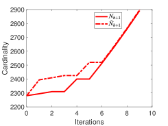
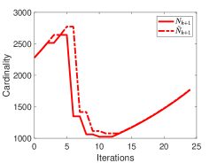
Fig. 2: Dataset a9a. Samples sizes $N_{k+1}$ and $\widetilde{N}_{k+1}$ versus iterations with $\mu=100/N$ (left) and $\mu=1$ (right), respectively, obtained with a single run of SIRTR. Classification errors: err = 0.187 with $\mu=100/N$, err = 0.174 with $\mu=1$.

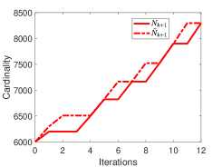
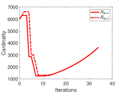
Fig. 3: Dataset mnist. Samples sizes $N_{k+1}$ and $\widetilde{N}_{k+1}$ versus iterations with $\mu=100/N$ (left) and $\mu=1$ (right), respectively, obtained with a single run of SIRTR. Classification errors: err = 0.154 with $\mu=100/N$, err = 0.167 with $\mu=1$.

4.2 Comparison with TRish

In this section we compare the performance of SIRTR with the so-called Trust-Region-ish algorithm (TRish) recently proposed in [20]. TRish is a stochastic gradient method based on a trust-region methodology. Normalized steps are used in a dynamic manner whenever the norm of the stochastic gradient is within a prefixed interval. In particular, the $k-$th iteration of TRish is given by

$$x_{k+1}=x_{k}-\begin{cases}\gamma_{1,k}\alpha_{k}g_{k},\quad&\text{if }\|g_{k}\|\in\left[0,\frac{1}{\gamma_{1,k}}\right)\\ \alpha_{k}\frac{g_{k}}{\|g_{k}\|},\quad&\text{if }\|g_{k}\|\in\left[\frac{1}{\gamma_{1,k}},\frac{1}{\gamma_{2,k}}\right]\\ \gamma_{2,k}\alpha_{k}g_{k},\quad&\text{if }\|g_{k}\|\in\left(\frac{1}{\gamma_{2,k}},\infty\right)\end{cases}$$

where $\alpha_{k}>0$ is the steplength parameter, $0<\gamma_{2,k}<\gamma_{1,k}$ are positive constants, and $g_{k}\in\mathbb{R}^{n}$ is a stochastic gradient estimate. This algorithm has proven to be particularly effective on binary classification and neural network training, especially if compared with the standard stochastic gradient algorithm [20, Section 4].

For our numerical tests, we implement TRish with subsampled gradients $g_{k}=\nabla f_{S}(x_{k})$ defined in (5). The steplength is constant, $\alpha_{k}=\alpha$, $\forall k\geq 0$, and $\alpha$ is chosen in the set $\{10^{-3},10^{-1},\sqrt{10^{-1}},1,\sqrt{10}\}$. Following the procedure in [20, Section 4], we use constant parameters $\gamma_{1,k}\equiv\gamma_{1}$, $\gamma_{2,k}\equiv\gamma_{2}$ and select $\gamma_{1},\,\gamma_{2}$ as follows. First, Stochastic Gradient algorithm [33] is run with constant steplength equal to $1$; second, the average norm $G$ of stochastic gradient estimates throughout the runs is computed; third $\gamma_{1},\,\gamma_{2}$ are set as $\gamma_{1}=\frac{4}{G}$, $\gamma_{2}=\frac{1}{2G}$.

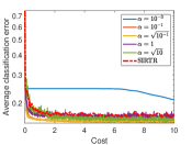
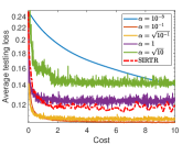
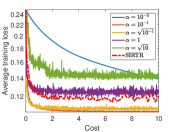
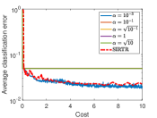
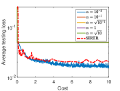
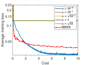
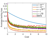
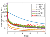
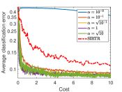
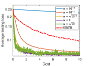
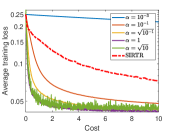
Fig. 4: From top to bottom row: datasets a9a, htru2, mnist, phishing. From left to right: Average classification error, testing loss, and training loss versus epochs.

First, we compare TRish with SIRTR on the nonconvex optimization problem (68), using a9a, htru2, mnist, and phishing as datasets (see Table 1). Based on the previous section, we equip SIRTR with $N_{0}=\lceil 0.01N\rceil$, $N_{k+1,g}=\lceil 0.1{N_{k+1}^{t}}\rceil$, $\widetilde{N}_{k+1}=\min\{N,\lceil 1.05N_{k}\rceil\}$, $\mu=100/N$. In TRish, the sample size $S$ of the stochastic gradient estimates is $\lceil 0.01N\rceil$, which corresponds to the first sample size used in SIRTR. We run each algorithm for ten epochs on the datasets a9a and htru2 using the null initial guess. We perform $10$ runs to report results on average.

After tuning, the parameter setting for TRish was $\gamma_{1}\approx 34.5805$, $\gamma_{2}\approx 4.3226$ for a9a, $\gamma_{1}\approx 57.9622$, $\gamma_{2}\approx 7.2453$ for htru2, $\gamma_{1}\approx 23.4376$, $\gamma_{2}\approx 2.9297$ for mnist, and $\gamma_{1}\approx 50.6409$, $\gamma_{2}\approx 6.3301$ for phishing. In Figure 4, we report the decrease of the (average) classification error, training loss $f_{N}$ and testing loss, $f_{N_{T}}(x)=\frac{1}{N_{T}}\sum_{i\in I_{N_{T}}}\phi_{i}(x)$, over the (average) number of full function and gradient evaluations required by the algorithms. From these plots, we can see that SIRTR performs comparably to the best implementations of TRish on a9a, htru2, mnist, while showing a good, though not optimal, performance on phishing.

In accordance to the experience in [20], all parameters $\gamma_{1}$ and $\gamma_{2}$ and $\alpha$ are problem-dependent. For instance, the best performance of TRish is obtained with $\alpha=10^{-1}$ for a9a and with $\alpha=10^{-3}$ for htru2, respectively; by contrast, SIRTR performs well with an unique setting of the parameters which is the key feature of adaptive stochastic optimization methods.

As a second test, we compare the performance of SIRTR and TRish on a different nonconvex optimization problem arising from nonlinear regression. Letting $\{(a_{i},b_{i})\}_{i=1}^{N}$ denote the training set, where $a_{i}\in\hbox{\rm I\kern-1.99997pt\hbox{\rm R}}^{n}$ and $b_{i}\in\hbox{\rm I\kern-1.99997pt\hbox{\rm R}}$ represent the feature vector and the target variable of the $i$-th example, respectively, we aim at solving the following problem

$$\min_{x\in\hbox{\rm I\kern-1.39998pt\hbox{\rm R}}^{n}}f_{N}(x)=\frac{1}{N}\sum_{i=1}^{N}\left(b_{i}-h(a_{i};x)\right)^{2},$$ (71)

where $h(\cdot;x):\hbox{\rm I\kern-1.99997pt\hbox{\rm R}}^{n}\rightarrow\hbox{\rm I\kern-1.99997pt\hbox{\rm R}}$ is a nonlinear prediction function.

For this second test, we use the air dataset [29], which contains $9358$ instances of (hourly averaged) concentrations of polluting gases, as well as temperatures and relative/absolute air humidity levels, recorded at each hour in the period March 2004 - February 2005 from a device located in a polluted area within an Italian city.

As in [22], our goal is to predict the benzene (C6H6) concentration from the knowledge of $n=7$ features, including carbon monoxide (CO), nitrogen oxides (NO_x), ozone (O₃), non-metanic hydrocarbons (NMHC), nitrogen dioxide (NO₂), air temperature, and relative air humidity. First, we preprocess the dataset by removing examples for which the benzene concentration is missing, reducing the dataset dimension from $9357$ to $8991$. Then, we employ $70\%$ of the dataset for training ($N=6294$), and the remaining $30\%$ for testing ($N_{T}=2697$). Since the concentration values have been recorded hourly, this means that we use the data measured in the first $9$ months for the training phase, and the data related to the last $3$ months for the testing phase. Finally, denoting with $D=(d_{ij})\in\hbox{\rm I\kern-1.99997pt\hbox{\rm R}}^{(N+N_{T})\times n}$ the matrix containing all the dataset examples along its rows, and setting

$$\begin{cases}m_{j}=\min\limits_{i=1,\ldots,N+N_{T}}{d_{ij}},\\ M_{j}=\max\limits_{i=1,\ldots,N+N_{T}}{d_{ij}}\end{cases},\quad j=1,\ldots,n,$$

we scale all data values into the interval $[0,1]$ as follows

$$d_{ij}=\frac{d_{ij}-m_{j}}{M_{j}-m_{j}},\quad i=1,\ldots,N+N_{T},\ j=1,\ldots,n.$$

We apply SIRTR and TRish on problem (71), where the prediction function $h(\cdot;x)$ is chosen as a feed-forward neural network based on a $7\times 5\times 1$ architecture (see [22] and references therein), with the two hidden layers both equipped with the linear activation function, and the output layer with the sigmoid activation function. We equip the two algorithms with the same parameter values employed in the previous tests, and run them $10$ times for $10$ epochs, using a random initial guess in the interval $[-\frac{1}{2},\frac{1}{2}]$.

In Figure 5, we report the decrease of the (average) training and testing losses provided by SIRTR and by TRish with different choices of the steplength $\alpha$, whereas in Figure 6 we show the benzene concentration estimations provided by the algorithms against the true concentration. These results confirm that the performances of SIRTR are comparable with those of TRish equipped with the best choice of the steplength and show the ability of SIRTR to automatically tune the steplength so as to obtain satisfactory results in terms of testing and training accuracy.

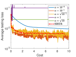
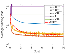
Fig. 5: Dataset air. Average testing loss (left) and training loss (right) versus epochs.

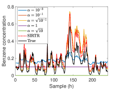
Fig. 6: Dataset air. Estimated concentrations during $10$ days ($240$ hours) compared to the true concentration (black solid line).

5 Conclusions

We proposed a stochastic gradient method coupled with a trust-region strategy and an inexact restoration approach for solving finite-sum minimization problems. Functions and gradients are subsampled and the batch size is governed by the inexact restoration approach and the trust-region acceptance rule. We showed the theoretical properties of the method and gave a worst-case complexity result on the expected number of iterations required to reach an approximate first-order optimality point. Numerical experience shows that the proposed method provides good results keeping the overall computational cost relatively low. Data Availability. The dataset CINA0 is no longer available in repositories but is available from the corresponding author on reasonable request. The other datasets analyzed during the current study are available in the repositories:
http://www.csie.ntu.edu.tw/~cjlin/libsvm,
http://yann.lecun.com/exdb/mnist,
https://archive.ics.uci.edu/ml/index.php Conflict of interest. The authors have not conflict of interest to declare.

References

• [1] A. S Bandeira, K. Scheinberg, L. N. Vicente, Convergence of trust-region methods based on probabilistic models, SIAM Journal on Optimization, 24(3), 1238–1264, 2014.
• [2] A.S. Berahas, L. Cao, K. Scheinberg, Global convergence rate analysis of a generic line search algorithm with noise, SIAM Journal on Optimization, 31(2), 1489–1518, 2021.
• [3] S. Bellavia, T. Bianconcini, N. Krejić, B. Morini, Subsampled first-order optimization methods with applications in imaging. Handbook of Mathematical Models and Algorithms in Computer Vision and Imaging. Springer, 1–35, 2021.
• [4] S. Bellavia, N. Krejić, B. Morini, Inexact restoration with subsampled trust-region methods for finite-sum minimization, Computational Optimization and Applications 76, 701–736, 2020.
• [5] S. Bellavia, G. Gurioli, B. Morini, Adaptive cubic regularization methods with dynamic inexact Hessian information and applications to finite-sum minimization, IMA Journal of Numerical Analysis, 41(1), 764-799, 2021.
• [6] S. Bellavia, G. Gurioli, B. Morini, Ph. L. Toint, Trust-region algorithms: probabilistic complexity and intrinsic noise with applications to subsampling techniques, arXiv:2112.06176, 2021.
• [7] S. Bellavia, G. Gurioli, B. Morini, Ph. L. Toint, Adaptive regularization for nonconvex optimization using inexact function values and randomly perturbed derivatives, Journal of Complexity, 68, Article number 101591, 2022.
• [8] D. P. Bertsekas, Nonlinear Programming, 3rd Edition, Athena Scientific, 2016.
• [9] G. E. Birgin, N. Krejić, J. M. Martínez, On the employment of Inexact Restoration for the minimization of functions whose evaluation is subject to programming errors, Mathematics of Computation 87(311), 1307–1326, 2018.
• [10] G. E. Birgin, N. Krejić, J. M. Martínez, Iteration and evaluation complexity on the minimization of functions whose computation is intrinsically inexact, Mathematics of Computation, 89, 253–278, 2020.
• [11] J. Blanchet, C. Cartis, M. Menickelly, K. Scheinberg, Convergence Rate Analysis of a Stochastic Trust Region Method via Submartingales, INFORMS Journal on Optimization, 1, 92–119, 2019.
• [12] L. Bottou, F. C. Curtis, J. Nocedal, Optimization Methods for Large-Scale Machine Learning, SIAM Review, 60(2), 223–311, 2018.
• [13] R. Bollapragada, R. Byrd, and J. Nocedal, Adaptive sampling strategies for stochastic optimization, SIAM Journal on Optimization, 28, 3312–3343, 2018.
• [14] R. H. Byrd, G. M. Chin, J. Nocedal, Y. Wu, Sample size selection in optimization methods for machine learning, Mathematical Programming, 134, 127–155, 2012.
• [15] C. Cartis, K. Scheinberg, Global convergence rate analysis of unconstrained optimization methods based on probabilistic models, Mathematical Programming 169, 337–375, 2018.
• [16] C. C. Chang, C. J. Lin, LIBSVM : a library for support vector machines, ACM Transactions on Intelligent Systems and Technology, 2:27:1–27:27, 2011 http://www.csie.ntu.edu.tw/~cjlin/libsvm
• [17] V. K. Chauhan, A. Sharma, K. Dahiya, Stochastic trust region inexact Newton method for large-scale machine learning, International Journal of Machine Learning and Cybernetics 11(7), 1541–1555, 2020.
• [18] R. Chen, M. Menickelly, K. Scheinberg, Stochastic optimization using a trust-region method and random models, Mathematical Programming, 169(2), 447–487, 2018.
• [19] F. E. Curtis, K. Scheinberg, Adaptive Stochastic Optimization: A Framework for Analyzing Stochastic Optimization Algorithms, IEEE Signal Processing Magazine, 37(5), 32–42, 2020.
• [20] F. E. Curtis, K. Scheinberg, R. Shi, A Stochastic Trust Region Algorithm Based on Careful Step Normalization, INFORMS Journal on Optimization 1(3), 200–220, 2019.
• [21] F. E. Curtis, K. Scheinberg, Optimization methods for supervised machine learning: From linear models to deep learning, Leading Developments from INFORMS Communities. INFORMS, 2017. 89–114.
• [22] S. De Vito, E. Massera, M. Piga, L. Martinotto, and G. Di Francia, On field calibration of an electronic nose for benzene estimation in an urban pollution monitoring scenario, Sensors and Actuators B, 129, 750–757, 2008.
• [23] I. Goodfellow, Y. Bengio, A. Courville, Deep learning, MIT Press, http://www.deeplearningbook.org, 2016.
• [24] R. M. Gower, M. Schmidt, F. Bach, P. Richtarik, Variance-reduced methods for machine learning. Proceedings of the IEEE, 108(11), 1968–1983, 2020.
• [25] R. Johnson, T. Zhang, Accelerating stochastic gradient descent using predictive variance reduction, Proceedings of the 26th International Conference on Neural Information Processing Systems 26, (NIPS 2013).
• [26] D. P. Kingma, J. Ba, Adam: A Method for Stochastic Optimization, Proceedings of the 3rd International Conference on Learning Representations (ICLR), 2015.
• [27] N. Krejić, J. M. Martínez, Inexact Restoration approach for minimization with inexact evaluation of the objective function, Mathematics of Computation, 85, 1775-1791, 2016.
• [28] Y. LeCun, L. Bottou, Y. Bengio, P. Haffner, Gradient-based learning applied to document recognition, Proceedings of the IEEE, 86(11):2278-2324, 1998. MNIST database available at http://yann.lecun.com/exdb/mnist
• [29] M. Lichman, UCI machine learning repository, https://archive.ics.uci.edu/ml/index.php, 2013.
• [30] J. M. Martínez and E. A. Pilotta, Inexact restoration algorithms for constrained optimization, Journal of Optimization Theory and Applications, 104, 135–163, 2000.
• [31] L. M. Nguyen, J. Liu, K. Scheinberg and M. Taka$\check{\text{c}}$, SARAH: A Novel Method for Machine Learning Problems Using Stochastic Recursive Gradient, Proceedings of the 34th International Conference on Machine Learning, PMLR 70:2613-2621, 2017.
• [32] C. Paquette, K. Scheinberg, A Stochastic Line Search Method with Expected Complexity Analysis, SIAM Journal on Optimization, 30 349–376, 2020.
• [33] H. Robbins, S. Monro, A Stochastic Approximation Method, The Annals of Mathematical Statistics, 22 400–407, 1951.
• [34] M. Schmidt, N. Le Roux, F. Bach, Minimizing Finite Sums with the Stochastic Average Gradient, Math. Program. 162, 83–112, 2017.
• [35] W. Xiaoyu, Y. X Yuan, Stochastic Trust Region Methods with Trust Region Radius Depending on Probabilistic Models, Journal of Computational Mathematics, 40(2), 294–334, 2022.
• [36] P. Xu, F. Roosta-Khorasani, M. W. Mahoney, Second-order optimization for non-convex machine learning: an empirical study, Proceedings of the 2020 SIAM International Conference on Data Mining.