\headersA Generalized CUR decomposition for matrix pairsPerfect Y. Gidisu and Michiel E. Hochstenbach
A Generalized CUR decomposition for matrix pairs††thanks: Version .\fundingThis work has received funding from the European Union’s Horizon 2020 research and innovation programme under the Marie Sklodowska-Curie grant agreement No 812912.
Perfect Y. Gidisu
Department of Mathematics and Computer Science, TU Eindhoven, The Netherlands, (, ).
p.gidisu@tue.nlm.e.hochstenbach@tue.nlMichiel E. Hochstenbach22footnotemark: 2
Abstract
We propose a generalized CUR (GCUR) decomposition for matrix pairs . Given matrices and with the same number of columns, such a decomposition provides low-rank approximations of both matrices simultaneously, in terms of some of their rows and columns. We obtain the indices for selecting the subset of rows and columns of the original matrices using the discrete empirical interpolation method (DEIM) on the generalized singular vectors.
When is square and nonsingular, there are close connections between the GCUR of and the DEIM-induced CUR of .
When is the identity, the GCUR decomposition of coincides with the DEIM-induced CUR decomposition of .
We also show similar connection between the GCUR of and the CUR of for a nonsquare but full-rank matrix , where denotes the Moore–Penrose pseudoinverse of . While a CUR decomposition acts on one data set, a GCUR factorization jointly decomposes two data sets. The algorithm may be suitable for applications where one is interested in extracting the most discriminative features from one data set relative to another data set. In numerical experiments, we demonstrate the advantages of the new method over the standard CUR approximation; for recovering data perturbed with colored noise and subgroup discovery.
With the proliferation of big data matrices, dimension reduction has become an important tool in many data analysis applications. There are several methods of dimension reduction for a given problem; however, the approximated data often consists of derived features that are either no longer interpretable or difficult to interpret in the original context. For example, while the singular value decomposition (SVD) provides an optimal approximation and compression of data, it may be difficult for domain experts to directly draw conclusions or interpret the singular vectors. In some applications, it is necessary to find a dimension reduction method that preserves the original properties (such as sparsity, nonnegativity, being integer-valued) of the data and ensures interpretability. In an attempt to solve this difficulty, one possibility for a low-rank representation of a given data matrix is to use a subset of the original columns and rows of the matrix itself: a CUR decomposition; see, e.g., Mahoney and Drineas [10]. The selected subsets of rows and columns capture the most relevant information of the original matrix.
A CUR decomposition of rank of a (square or rectangular) matrix is of the form
(1)
Here, is an (where ) index selection matrix with some columns of the identity matrix that selects certain columns of .
Similarly, is an matrix with columns of
that selects certain rows of ; so is and is . We construct the matrix in such a way that the decomposition has some desirable approximation properties that we will discuss in Section4. (In line with [28], we will use the letter rather than .) It is also possible to select a different number of columns and rows; here, will not be of dimension . It is worth noting that given , this decomposition is not unique; there are several ways to obtain this form of approximation to with different techniques of choosing the representative columns and rows. Many algorithms for this decomposition using the truncated SVD (TSVD) as a basis have been proposed [5, 34, 22, 10]. In [25], Sorensen and Embree present a CUR decomposition inspired by a discrete empirical interpolation method (DEIM) on a TSVD. Let the rank- TSVD be
(2)
where the columns of and are orthonormal,
while is diagonal with nonnegative elements. Throughout the paper we assume a unique truncated singular value decomposition, i.e., the th singular value is not equal to the st singular value.
There is extensive work on CUR-type decompositions in both numerical linear algebra and theoretical computer science. In this paper, we develop a generalized CUR decomposition (GCUR) for matrix pair, for any two matrices and with the same number of columns: is , is and of full rank. The intuition behind this generalized CUR decomposition is that we can view it as a CUR decomposition of relative to . As we will see in Proposition4.2, when is square and nonsingular, the GCUR decomposition has a close connection with the CUR of . The GCUR is also applicable to nonsquare matrices ; see the examples in Section5. We show in Proposition4.2 that if is nonsquare but of a full rank, we still have a close connection between the CUR decomposition of (where denotes the pseudoinverse of ) and the GCUR decomposition. Another intuition for this GCUR decomposition comes from a footnote remark by Mahoney and Drineas [22, p. 700]: “for data sets in which a low-dimensional subspace obtained by the SVD failed to capture category separation, CUR decomposition performed correspondingly poorly”. This is evident in Section5.
Inspired by the work of Sorensen and Embree [25], we present a generalized CUR decomposition using the discrete empirical interpolation method.
The DEIM algorithm for interpolation indices, presented in [7], is a discrete variant of empirical interpolation proposed in [3] as a method for model order reduction for nonlinear dynamical systems. In [25], the authors used DEIM as an index selection technique for constructing the and factors of a CUR decomposition. The DEIM algorithm independently selects the column and row indices based on the right and left singular vectors of a data matrix , respectively. Our new GCUR method uses the matrices obtained from the GSVD instead. Besides using DEIM on the GSVD for index selection, we can also use other CUR-type index selection strategies for the GCUR (see also Section6). The proposed method can be used in situations where a low-rank matrix is perturbed with noise, where the covariance of the noise is not a multiple of the identity matrix. It may also be appropriate for applications where one is interested in extracting the most discriminative information from a data set of interest relative to another data set. We will see examples of these in Section5.
Example 1.1.
The following simple example shows that using the matrices obtained from the GSVD instead of the SVD can lead to more accurate results when approximating data with colored noise. Unlike white noise, colored noise is correlated. In discrete time, the noise samples of colored noise need not be independent. In terms of the Fourier transform, some frequencies are more present than others.
As in [17, p. 55] and [24], we use the term “colored noise” for noise of which the covariance matrix is not a multiple of the identity.
We consider a full-rank matrix representing low-rank data, and want to try to recover an original low-rank matrix perturbed by colored noise. Our test matrix is a rank-2 matrix of size perturbed by additive colored noise with a given desired covariance structure. We take
We generate the colored noise as an additive white Gaussian noise multiplied by the Cholesky factor of the desired covariance matrix. The matrix is, as a result, a sum of a rank-2 matrix and a correlated Gaussian noise matrix. We compute the SVD of both and . The dominant left singular vectors of are denoted by while those of are . We also compute the GSVD of and denote the dominant left generalized singular vectors by . Since we are interested in recovering , we examine the angle between the leading -dimensional exact left singular subspace Range and its approximations Range and Range. We generate 1000 different test cases and take the average of the subspace angles.
Table1 shows the results for and three different noise levels. We observe that the approximations obtained using the GSVD in terms of subspace angles are more accurate than those from the SVD; about 40% gain in accuracy. This illustrates the potential advantage of using generalized singular vectors in the presence of colored noise.
Table 1: The average angle between the leading two-dimensional exact singular subspace Range (which is the range of ) and its approximations Range and Range, for different values of the noise level . The subspaces Range and Range are from the SVD of and the GSVD of , respectively.
Method
Subspace angle
SVD
GSVD
SVD
GSVD
SVD
GSVD
Inspired by this example, we expect that the GCUR compared to the CUR may produce better approximation results in the presence of non-white noise, as it is based on the GSVD instead of the SVD. We show in Section5 that the GSVD and the GCUR may provide equally good approximation results even when we use an inexact Cholesky factor.
Throughout the paper, we denote the 2-norm by and the infinity-norm by . We use MATLAB notation to index vectors and matrices; thus, denotes the columns of whose corresponding indices are in vector .
Outline.
We give a brief introduction to the generalized singular value decomposition in Section2. We also discuss the truncated GSVD and its approximation error bounds. We summarize the DEIM technique we use for index selection in Section3. Section4 introduces the new generalized CUR decomposition with an analysis of its error bounds. In Algorithm2, we present a DEIM-type GCUR decomposition algorithm. Results of numerical experiments are presented in Section5, followed by conclusions in Section6.
2 Generalized singular value decomposition
The GSVD appears throughout this paper since it is a key building block of the proposed algorithm. This section gives a brief overview of this decomposition. The original proof of the existence of the GSVD has first been introduced by Van Loan in [31]. Paige and Saunders [23] later presented a more general formulation without any restrictions on the dimensions except for both matrices to have the same number of columns. Other formulations and contributions to the GSVD have been proposed in [26, 29, 32]. For our applications in this paper, let and with both and . Following the formulation of the GSVD proposed by Van Loan [31]: there exist matrices , with orthonormal columns and a nonsingular such that
(3)
where . Although traditionally the ratios are in a nondecreasing order, for our purpose we will instead maintain a nonincreasing order. The matrices and contain the left generalized singular vectors of and , respectively; and similarly, contains the right generalized singular vectors and is identical for both decompositions. While the SVD provides two sets of linearly independent basis vectors, the GSVD of gives three new sets of linearly independent basis vectors (the columns of and ) so that the two matrices and are diagonal when transformed to these new bases.
We note that only the reduced GSVD is needed, so that we can assume that , , and and are .
Our analysis is based on the following formulation of the GSVD presented in [32]. Let in the GSVD of (3), then and . Let us characterize matrix . (In fact, Matlab’s gsvd routine renders instead of .) Since
(4)
this implies that we have the following congruence transformations
From the above, it follows that has the same inertia as and the same holds for and (here this mainly gives information on the number of zero eigenvalues).
We also see that, provided and are of full-rank, these similarity transformations hold:
(5)
The columns of the matrix are therefore the eigenvectors for both and its inverse . The GSVD avoids the explicit formation of the cross-product matrices and (see also Section5).
Truncated GSVD.
In some practical applications it could be of interest to approximate both matrices by other matrices , said truncated, of a specific rank . To define the truncated GSVD (TGSVD) let us partition the following matrices
(6)
For use in Section4, we define TGSVD for as (cf. [17, (2.34)])
(7)
where .
then it follows that
The following proposition is useful for understanding the error bounds for the GCUR. In line with [16, p. 495],
let and be the singular values of matrix and , respectively (cf. also (2)). The first and second statements of the following proposition are from [16]; while the third statement may not be present in the literature yet, it is straightforward.
Proposition 2.1.
Let as in (3), with , then for (see, e.g., [16, pp. 495–496])
so
Moreover,
Proof 2.2.
This follows from (4) and the well-known property that, for the product of two matrices we have (see, e.g., [20, p. 89]).
The results above are relevant tools for the analysis and understanding of generalized CUR and its error bounds which we will introduce in Section4.
3 Discrete empirical interpolation method
We now summarize the tool from existing literature [25, 7] that we use to select columns and/or rows from matrices. Besides the GSVD, the DEIM algorithm plays an important role in the proposed method. The DEIM procedure works on the columns of a specified basis vectors sequentially. The basis vectors must be linearly independent. Assuming we have a full-rank basis matrix with , to select rows from , the DEIM procedure constructs an index vector such that it has non-repeating values in . Defining the selection matrix as an identity matrix indexed by , i.e., and (cf. [25]), we have an interpolatory projector defined through the DEIM procedure as
We can show that is nonsingular (see [25, Lemma 3.2]). The term “interpolatory projector” stems from the fact that for any we have
implying the projected vector matches in the entries [25].
To select the indices contained in , the columns of are considered successively. The first interpolation index corresponds to the index of the entry with the largest magnitude in the first basis vector. The rest of the interpolation indices are selected by removing the direction of the interpolatory projection in the previous basis vectors from the subsequent one and finding the index of the entry with the largest magnitude in the residual vector. The index selection using DEIM is limited by the rank of the basis matrix, i.e., the number of indices selected can be no more than the number of vectors available.
To form , let denote the th column of and be the matrix of the first columns of . Similarly, let contain the first entries of , and let . More precisely, we define such that
and the th interpolatory projector as
To select , remove the component from by projecting onto indices {, …, }, thus
then take the index of the entry with the largest magnitude in the residual, i.e., such that
As noted in [7], in case of a tie e.g., for , the smaller index is picked. As in DEIM-induced CUR decomposition [25, p. A1458], this process will never produce duplicate indices. In a nutshell, we find the indices via a non-orthogonal Gram–Schmidt-like process (oblique projections) on the -vectors. Since the input vectors are linearly independent, the residual vector is guaranteed to be nonzero. This DEIM algorithm forces the selection matrix to find linearly independent rows of such that the local growth of is kept modest via a greedy search [7, p. 2748] as implemented in Algorithm1.
Input: , with (linearly independent columns)
Output: Indices with distinct entries in
1:
2:
3:fordo
4:
5:
6:
7: =
8:
9:endfor
Although the DEIM index selection procedure is basis-dependent, if the interpolation indices are determined, the DEIM interpolatory projector is independent of the choice of basis spanning the space Range.
Proposition 3.1.
([7, Def. 3.1, (3.6)] ).
Let be an orthonormal basis of Range where for , then
This proposition allows us to take advantage of the special properties of an orthonormal matrix in cases where our input basis matrix is not (see Proposition4.7).
4 Generalized CUR decomposition and its approximation properties
In this section we describe the proposed generalized CUR decomposition and provide a theoretical analysis of its error bounds.
4.1 Generalized CUR decomposition
We now introduce a new generalized CUR decomposition of matrix pairs , where is and is , and is of full rank. This GCUR is inspired by the truncated generalized singular value decomposition for matrix pairs, as reviewed in Section2. We now define a generalized CUR decomposition (cf. (1)).
Definition 4.1.
Let be and be and of full rank, with and .
A generalized CUR decomposition of of rank is a matrix approximation of
and expressed as
(8)
Here , , and are index selection matrices .
It is key that the same columns of and are selected;
this gives a coupling between the decomposition of and .
The matrices and are subsets of the columns and rows, respectively, of the original matrices. In the rest of the paper, we will mainly focus on the matrix ; we can perform a similar analysis for the matrix (see also the comments at the end of this section). As in Section3, we again have the vectors as the indices of the selected rows and columns such that and , where and . The choice of and is based on the transformation matrices from the rank- truncated GSVD.
Given and , the middle matrix can be constructed in different ways to satisfy certain desirable approximation properties. In [25], the authors show how setting leads to a CUR decomposition corresponding to the columns and rows of . Instead, following these authors [25] and others [22, 27], we choose to construct the middle matrix as . This option, as shown by Stewart [27], minimizes for a given and . Computing the middle matrix as such yields a decomposition that can be viewed as first projecting the columns of onto and then projecting the result onto the row space of , both steps being optimal for the 2-norm error.
The following proposition establishes a connection between the DEIM-GCUR of and the DEIM-CUR of and for a square and nonsingular and a nonsquare but full-rank , respectively.
Proposition 4.2.
(i) If is a square and nonsingular matrix, then the selected row and column indices from the CUR decomposition of are the same as index vectors and obtained from the GCUR decomposition of , respectively.
(ii) Moreover, in the special case where , the GCUR decomposition of coincides with the CUR decomposition of , in that the factors and of are the same for both methods: the first line of (8) is equal to (1).
(iii) In addition, if is nonsquare but of a full rank, we have a connection as in (i) between the indices from the CUR decomposition of and the index vectors and obtained from the GCUR decomposition of .
Proof 4.3.
(i) We start with the GSVD (4). If is square and nonsingular, then the SVD of can be expressed in terms of the GSVD of , and is equal to [13].
Therefore, the row index selection matrix from the SVD of is equal to from the GSVD of ; and similarly the column index selection matrix obtained from the SVD of is equal to , since they are determined using and , respectively.
(ii) If , then from the second line of (4) we have that . This implies that the index of the largest entries in the columns of are the same as that of .
In this special case of , we have , so then the left and right singular vectors of are contained in the and matrices from the GSVD of , respectively. Hence the selection matrix in (8) obtained by performing DEIM on is the same as the selection matrix in (1) obtained by applying DEIM to the right singular vectors of .
(iii) If is nonsquare but of full rank , then we still have a similar connection between the GSVD of and the SVD of because of the following. Since the factors in the reduced GSVD are of full rank, we have . This means that , so the index vectors and from GCUR of are equivalent to the selected column and row indices from CUR of , respectively.
It is worth noting that Proposition4.2 holds for DEIM-based CUR and GCUR algorithms. For alternative ways of constructing CUR and GCUR decompositions (see Section6) these properties may not hold.
Although we can obtain indices of a CUR decomposition of using the GCUR of , the converse does not hold. We emphasize that we need the GSVD for the GCUR decomposition and cannot use the SVD of or instead, since the GCUR decomposition requires the matrix from (7) to find the column indices. While we used the generalized singular vectors here, in principle one could use other vectors, e.g., an approximation to the generalized singular vectors.
To build the decomposition, it is relevant to know the dominant rows and columns of and in their rank- approximations. Given that and are rank- approximations of and , respectively, how should the columns and rows be selected? Algorithm2 is a summary of the procedure. (The backslash operator used in Algorithm2 is a Matlab type notation for solving linear systems and least-squares problems.)
We note that we can parallelize the work in 3, 4, 5, 6, 7 and 8 since it consists of three independent runs of DEIM. Also, if we are only interested in approximating the matrix from the pair , we can omit 5 and 8 as well as the second part of 10; thus saving computational cost.
In some applications, one might be interested in a generalized interpolative decomposition, of which the column and row versions are of the form
(9)
Here is and is ; similar remarks hold for and . As noted in [25], since the DEIM index selection algorithm identifies the row and column indices independently, this form of decomposition is relatively straightforward.
In terms of computational complexity, the dense GSVD method requires work and the three runs of DEIM together require work, so the overall complexity of the algorithm is dominated by the construction of the GSVD. (This might suggest iterative GSVD approaches; see Section6.)
Algorithm 2 DEIM type GCUR decomposition
Input: , (where and ), desired rank
Output: A rank- generalized CUR decomposition
,
1:(according to nonincreasing generalized singular values)
2:fordo
3:(Iteratively pick indices)
4:
5:(Update new columns)
6: )
7: )
8: )
9:endfor
10: ,
The pseudocode in Algorithm2 assumes the matrices from the GSVD (i.e., , , and ) corresponds to a nonincreasing order of the generalized singular values.
In generalizing the DEIM-inspired CUR decomposition, we also look for a generalization of the related theoretical results. While the results presented in [25] express the error bounds in terms of the optimal rank- approximation, for our generalized CUR factorization, the most relevant quantity is the rank- GSVD approximation. In the following subsection, we present theoretical results for bounding the GCUR approximation error.
4.2 Error Bounds in terms of the SVD approximation
The error bounds for any rank- matrix approximation are usually expressed in terms of the rank- SVD approximation error. We will show a result of this type in the following proposition and also discuss its limitations.
We introduce the following notation: let be the SVD of (see (2)), where contains the largest right singular vectors.
Let be an matrix with orthonormal columns. It turns out in both [25] and this section that is a central quantity in the analysis. In the DEIM-induced CUR decomposition work [25], we take the right singular vectors to be , but here we study this quantity for general . In our context, we are particularly interested in as the orthogonal basis of the matrix in (7).
Denote and . Recall that the are the singular values of .
Proposition 4.4.
Let be an matrix with orthonormal columns, and let contain the largest right singular vectors of . Then
More precisely, we have
Proof 4.5.
The lower bound follows from the SVD; the optimal is .
We can derive the upper bounds from
Furthermore, more specifically,
The significance of this result is that may be close to when captures the largest singular vectors of well. For instance, in the standard CUR, is equivalent to so the quantity equals 0. If the matrix from (4) is close to the identity or is a scaled identity, we expect that will be approximately zero. However, this sine will generally not be small, as we illustrate by the following example.
Example 4.6.
Let , and .
Denote by the th standard basis vector.
Then clearly , while the largest right generalized singular vector is equal to the largest right singular vector of , and hence .
This implies that is large.
4.3 Error Bounds in terms of the GSVD approximation
With the above results in mind, instead of using the rank- SVD approximation error, we will derive error bounds for (see (8)) in terms of the error bounds of a rank- GSVD approximation of (see Proposition2.1).
The matrices and are of full-rank determined by the row and column index selection matrices and , respectively and . From Algorithm2, we know that and are derived using the columns of the matrices and , respectively, corresponding to the largest generalized singular value (see (7)).
We use the interpolatory projector given in Proposition3.1. Therefore instead of (see (4)), we use its orthonormal basis , to exploit the properties of an orthogonal matrix.
We will now analyze the approximation error between and its interpolatory projection . The proof of the error bounds for the proposed method closely follows the one presented in [25].
The second inequality of the first statement of Proposition4.7 is in [25, Lemma 4.1]. The first inequality of the first statement is new but completely analogous. In the second statement, we use the GSVD.
For the analysis, we need the following QR-decomposition of (see (6)):
(10)
where we have defined
(11)
This implies that
Proposition 4.7.
(Generalization of [25, Lemma 4.1])
Given and with orthonormal columns where , let be a selection matrix and be nonsingular. Let , then
In particular, if is an orthonormal basis for , the first columns of , then
Proof 4.8.
We have that implies .
Therefore,
and also
Note that, since , we know that and , and hence (see, e.g., [30])
With , , and we have
and hence
This implies
and
Let us now consider the operation on the left-hand side of . Given the set of interpolation indices determined from , and for a nonsingular , we have the DEIM interpolatory projector . Since consists of the dominant left generalized singular vectors of and has orthonormal columns, it is not necessary to perform a QR-decomposition as we did in Proposition4.7.
The following proposition is analogous to Proposition4.7. The results are similar to those in [25, p. A1461] except that here, we use the approximation error of the GSVD instead of the SVD.
Proposition 4.9.
Given with orthonormal columns where , let be a selection matrix and be nonsingular. Furthermore, let , then, with as in (11),
Proof 4.10.
We have
Similar to before, since , we know that and hence
Since we get
and , from which the result follows.
We will now use Propositions4.7 and 4.9 to find a bound for the approximation error of the GCUR of relative to . As in [25] we first show in the following proposition that the error bounds of the interpolatory projection of onto the chosen rows and columns apply equally to the orthogonal projections of onto the same row and column spaces.
Proposition 4.11.
(Generalization and slight adaptation of [25, Lemma 4.2]) Given the selection matrices , , let and . Suppose that and are full rank matrices with , and that and are nonsingular. With and as in (10)–(11), we have the bound for the orthogonal projections of onto the column and row spaces:
Proof 4.12.
This proof is a minor modification of that of [25, Lemma 4.2]; we closely follow their proof technique. With of full rank, we have . With this, the orthogonal projection of onto Range can be stated as
Let , note that since is an oblique projector on Range. We can rewrite as .
Hence the error in the orthogonal projection of will be
.
Since , we have
therefore
With being nonsquare, (see, e.g., [30])
and from Proposition4.7, we have
In a similar vein, with and we have and the error in the orthogonal projection of is , where , so that
and
This result helps to prove an error bound for the GCUR approximation error. For the following theorem, we again closely follow the approach of [25] which also follows a procedure in [22].
As stated in Definition4.1 the middle matrix can be computed as .
Theorem 4.13.
(Generalization of [25, Thm. 4.1]) Given and , from (7), let and be selection matrices so that and are of full rank. Let be the -factor of , and and as in (10)–(11). Assuming and are nonsingular, then with the error constants
we have
Proof 4.14.
By the definition of , we have
using the triangle inequality, it follows that
and the fact that is an orthogonal projection with ,
The last line of Theorem4.13 can be related to the results in [25, Thm. 4.1]; both theorems have the factors and . In [25], the error of the CUR approximation of is within a factor of of the best rank- approximation, obtained from the SVD. Theorem4.13 provides a bound in terms of from the GSVD (3) and the additional factors and . The results presented in this section suggest that a good index selection procedure that yields small quantities and is desirable. For a bound on , given , Chandrasekaran and Ipsen [6] have developed an efficient algorithm that computes a rank-revealing QR factorization
such that . To bound , we start by restating the results of [17, Thm. 2.3] for the GSVD of . Defining
We know from Eq.4 that , so we can restate the above inequality as . Given the partitioning and QR factorization of in Eq.10,
we have that
In fact, we note that we can exploit the tighter bound to improve the bound on accordingly.
We note that where these results have been presented for matrix in (8), similar results can be obtained for . The following error bound for the approximation of is analogous to Theorem4.13. As noted in Definition4.1, the selection matrix is similar for the GCUR decomposition of and therefore we have the quantity in the error bound of both factorizations:
It is worth nothing that these bounds hold irrespective of the approach used to select the row and column indices. Since the GCUR algorithm presented in this paper is DEIM-based,
[25] provides deterministic bounds:
We refer to [25, Lemma 4.4] for the constructive proofs, and will give an example with the various quantities in Section5.
5 Numerical experiments
We now present the results of a few numerical experiments to illustrate the performance of GCUR for low-rank matrix approximation. For the first two experiments, we consider a case where a data matrix is corrupted by a random additive noise and the covariance of this noise (the expectation of ) is not a multiple of the identity matrix. We are therefore interested in a method that can take the actual noise into account. Traditionally, a pre-whitening matrix (where is the Cholesky factor of the noise’s covariance matrix) may be applied to the perturbed matrix [17], so that one can use SVD-based methods on the transformed matrix. With a GSVD formulation, the pre-whitening operation becomes an integral part of the algorithm [18]; we do not need to explicitly compute and transform the perturbed matrix. We show in the experiments that using SVD-based methods without pre-whitening the perturbed data yields less accurate approximation results of the original matrix.
For the last two experiments, we consider a setting with two data sets collected under different conditions, e.g., treatment and control experiment where the former has distinct variation caused by the treatment; signal-free and signal recordings with the signal-free data set containing only noise. We are interested in exploring and identifying patterns and discriminative features that are specific to one data set.
{experiment}
This experiment is an adaptation of experiments in [17, p. 66: Sect. 3.4.4] and [25, Ex. 6.1]; see also the motivating example in Section1. We construct matrix to be of a known modest rank. We then perturb this matrix with a noise matrix whose entries are correlated. Given , we evaluate and compare the GCUR and the CUR decomposition on in terms of recovering the original matrix . Specifically, the performance of each decomposition is assessed based on the 2-norm of the relative matrix approximation error i.e., , where is the approximated low-rank matrix.
We present the numerical results for four noise levels; thus where is the parameter for the noise level and is a randomly generated correlated noise. We first generate a sparse, nonnegative rank-50 matrix , with and , of the form
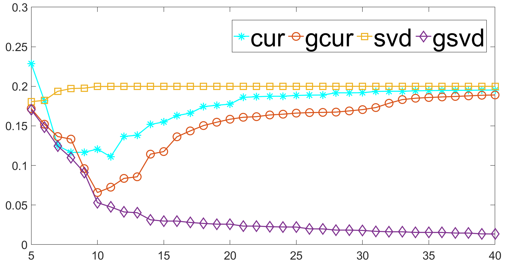
where and are sparse vectors with random nonnegative entries (i.e., and , just as in [25]. Unlike [25] we then perturb the matrix with a correlated Gaussian noise whose entries have zero mean and a Toeplitz covariance structure (in MATLAB , , , , and and , , , . We compute the SVD of and the GSVD of to get the input matrices for the CUR and the GCUR decomposition respectively. Figures1a, 1b, 1c and 1d compare the relative errors of the proposed DEIM-GCUR (see Algorithm2) and the DEIM-CUR (see Algorithm1) for reconstructing the low-rank matrix for different noise levels.
We observe that for higher noise levels the GCUR technique gives a more accurate low-rank approximation of the original matrix . The DEIM-GCUR scheme seems to perform distinctly well for higher noise levels and moderate values of . As indicated in Section4, the GCUR method is slightly more expensive since it requires the computation of the TGSVD instead of the TSVD. We observe that, as approaches rank, the relative error of the TGSVD continues to decrease; this is not true for the GCUR. We may attribute this phenomenon to the fact that the relative error is saturated by the noise considering we pick actual columns and rows of the noisy data. Since indicates the relative noise level, it is, therefore, natural that for increasing , the quality of the TSVD approximation rapidly approaches . For this experiment, we assume that an estimate of the noise covariance matrix is known and therefore we have the exact Cholesky factor; we stress that this may not always be the case.
Therefore, we now show an example where we use an inexact Cholesky factor . We derive by multiplying all off-diagonal elements of the exact Cholesky factor by factors which are uniformly random from the interval . Here, the experiment setup is the same as described above with the difference that we compute the GSVD of instead. In Figs.2a and 2b, we observe that the GCUR and the GSVD still deliver good approximation results even for an inexact Cholesky factor which may imply that we do not necessarily need the exact noise covariance.
(a) .
(b) .
(c) .
(d) .
Figure 1: Accuracy of the DEIM-GCUR approximations compared with the standard DEIM-CUR approximations in recovering a sparse, nonnegative matrix perturbed with correlated Gaussian noise (Section5) using exact Cholesky factor of the noise covariance. The relative errors (on the vertical axis) as a function of rank (on the horizontal axis) for , , , , respectively.
(a) .
(b) .
Figure 2: Accuracy of the DEIM-GCUR approximations compared with the standard DEIM-CUR approximations in recovering a sparse, nonnegative matrix perturbed with correlated Gaussian noise (Section5) using an inexact Cholesky factor of the noise covariance. The relative errors (on the vertical axis) as a function of rank (on the horizontal axis) for , , respectively.
We conclude this experiment by an illustration of the various quantities in Theorem4.13.
In Fig.3, we see that the upper bound in Theorem4.13 may be a rather crude bound on the true GCUR error. As in [25, Fig. 4], the quantities and may differ considerably in magnitude. While steadily decreases, seems to stabilize as increases.
Figure 3: Various quantities from Theorem4.13: error constants (red dashed) and (red solid); multiplicative factors (green solid) and (green dashed); the GCUR true error of approximating in Section5 (blue solid) and its upper bound (blue dashed).
{experiment}
For this experiment, we maintain all properties of matrix mentioned in the preceding experiment except for the column size that we reduce to 10000 (i.e., ) and instead of a sparse nonnegative matrix , we generate a dense random matrix . As in [25, Ex. 6.2], we also modify so that there is a significant drop in the 10th and 11th singular values. The matrix is now of the form
For each fixed and , we repeat the process 100 times and then compute the average relative error. The results in Table2 show that the advantage of the GCUR over the CUR still remains even when singular values of the original matrix decrease more sharply. We observe that the difference in the relative error of the GCUR and the CUR is quite significant when the rank of the recovered matrix is lower than that of (i.e., ).
Table 2: Comparison of the qualities of the TSVD, TGSVD, CUR, and GCUR approximations as a function of index and noise level in Section5. The relative errors are the averages of 100 test cases.
Method
10
TSVD
TGSVD
CUR
GCUR
15
TSVD
TGSVD
CUR
GCUR
20
TSVD
TGSVD
CUR
GCUR
30
TSVD
TGSVD
CUR
GCUR
The higher the noise level, the more advantageous the GCUR scheme may be over the CUR one. Especially for moderate values of such as , the GCUR approximations are of better quality than those based on the CUR. For higher values of such as , the approximation quality of the CUR and GCUR method become comparable since they both start to pick up the noise in the data columns. In this case, the GCUR does not improve on the CUR. Since it is a discrete method, picking indices for columns instead of generalized singular vectors, we see that the GCUR method yields worse results than the TGSVD approach.
{experiment}
Our next experiment is adapted from [1]. We create synthetic data sets which give an intuition for settings where the GSVD and the GCUR may resolve the problem of subgroups. Consider a data set of interest (target data), , containing 400 data points in a 30-dimensional feature space. This data set has four subgroups ( blue, yellow, orange, and purple), each of 100 data points. The first 10 columns for all 400 data points are randomly sampled from a normal distribution with a mean of 0 and a variance of 100. The next 10 columns of two of the subgroups ( blue and orange) are randomly sampled from a normal distribution with a mean of 0 and a unit variance while the other two subgroups ( yellow and purple) are randomly sampled from a normal distribution with a mean of 6 and a unit variance. The last 10 columns of subgroups blue and yellow are sampled from a normal distribution with a mean of 0 and a unit variance and those of purple and orange are sampled from a normal distribution with a mean of 3 and a unit variance.
One of the goals of the SVD (or the related concept principal component analysis) in dimension reduction is to find a low-dimensional rotated approximation of a data matrix while maximizing the variances.
We are interested in reducing the dimension of . If we project the data onto the two leading right singular vectors, we are unable to identify the subgroups because the variation along the first 10 columns is significantly larger than in any other direction, so some combinations of those columns are selected by the SVD.
Suppose we have another data set (a background data set), whose first 10 columns are sampled from a normal distribution with a mean of 0 and a variance of 100, the next 10 columns are sampled from a normal distribution with a mean of 0 and a variance of 9 and the last 10 columns are sampled from a normal distribution with a mean of 0 and a unit variance. The choice of the background data set is key in this context. Generally, the background data set should have the structure we would like to suppress in the target data, which usually corresponds to the direction with high variance but not of interest for the data analysis [1]. With the new data, one way to extract discriminative features for clustering the subgroups in is to maximize the variance of while minimizing that of , which leads to a trace ratio maximization problem [8]
where and or .
By doing this, the first dimensions are less likely to be selected because they also have a high variance in data set . Instead, the middle and last dimensions of are likely to be selected as they have the dimensions with the lowest variance in , thereby allowing us to separate all four subgroups. The solution to the above problem is given by the (right) eigenvectors of corresponding to the largest eigenvalues (cf., [12, pp. 448–449]); this corresponds to the (“largest”) right generalized singular vectors of (the transpose of (5)). As seen in Fig.4, projecting onto the leading two right generalized singular vectors produces a much clearer subgroup separation (top-right figure) than projecting onto the leading two right singular vectors (top-left figure). Therefore, we can expect that a CUR decomposition based on the SVD will also perform not very well with the subgroup separation. In the bottom figures is a visualization of the data using the first two important columns selected using the DEIM-CUR (left figure) and the DEIM-GCUR (right figure). To a large extent, the GCUR is able to differentiate the subgroups while the CUR fails to do so. We investigate this further by comparing the performance of subset selection via DEIM-CUR on (Algorithm1) and DEIM-GCUR on (Algorithm2) in identifying the subgroup or class representatives of ; we select a subset of the columns of (5 and 10) and compare the classification results of each method. We center the data sets by subtracting the mean of each column from all the entries in that column. Given the class labels of the subgroups, we perform a ten-fold cross-validation (i.e., split the data points into 10 groups and for each unique group take the group as test data and the rest as training [21, p. 181]) and apply two classifiers on the reduced data set: ECOC (Error Correcting Output Coding) [9] and classification tree [2] using the functions fitcecoc and fitctree with default parameters as implemented in MATLAB. It is evident from Table3 that the TGSVD and the GCUR achieve the least classification error rate, e.g., for reducing the dimension from 30 to 10; 0% and 6.3% respectively, using the ECOC classifier and 0% and 9.5% respectively, using the tree classifier. The standard DEIM-CUR method achieves the worst classification error rate.
Figure 4: (Top-left) We project the synthetic data containing four subgroups onto the first two dominant right singular vectors. The lower-dimensional representation using the SVD does not effectively separate the subgroups. In the bottom-left figure, we visualize the data using the first two columns selected by DEIM-CUR. (Top-right) We illustrate the advantage of using GSVD by projecting the data onto the first two dominant right generalized singular vectors corresponding to the two largest generalized singular values. In the bottom-right figure, we visualize the data using the first two columns selected by DEIM-GCUR. The lower-dimensional representation of the data using the GSVD-based methods clearly separates the four clusters while the SVD-based methods fail to do so.
Table 3: -Fold loss is the average classification loss overall 10-folds using SVD, GSVD, CUR, and GCUR as dimension reduction in Section5. The second and third columns give information on the number of columns selected from the data set using the CUR and GCUR plus the number of singular and generalized singular vectors considered for the ECOC classifier. Likewise, the fifth and sixth columns for the tree classifier.
Method
-Fold Loss
Method
-Fold Loss
5
10
5
10
TSVD+ECOC
TSVD+Tree
TGSVD+ECOC
TGSVD+Tree
CUR+ECOC
CUR+Tree
GCUR+ECOC
GCUR+Tree
{experiment}
We will now investigate the performance of the GCUR compared to the CUR on a higher-dimensional public data sets. The data sets consists of single-cell RNA expression levels of bone marrow mononuclear cells (BMMCs) from an acute myeloid leukemia (AML) patient and two healthy individuals. We have data on the BMMCs before stem-cell transplant and the BMMCs after stem-cell transplant. We preprocess the data sets as described by the authors in [4]111https://github.com/PhilBoileau/EHDBDscPCA/blob/master/analyses/ keeping the 1000 most variable genes measured across all 16856 cells (patient-035: 4501 cells and two healthy individuals; one of 1985 cells and the other of 2472 cells). The data from the two healthy patients are combined to create a background data matrix of dimension and we use patient-035 data set as the target data matrix of dimension . Both data matrices are sparse: the patient-035 data matrix has 1,628,174 nonzeros; i.e., about 36% of all entries are nonzero and the background data matrix has 1,496,229 nonzeros; i.e., about 34% of all entries are nonzero. We are interested in exploring the differences in the AML patient’s BMMC cells pre- and post-transplant.
We perform SVD, GSVD, CUR and GCUR on the target data (AML patient-035) to see if we can capture the biologically meaningful information relating to the treatment status. For the GSVD and the GCUR procedure the background data is taken into account. As evident in Fig.5, the GSVD and the GCUR produce almost linearly separable clusters which corresponds to pre- and post-treatment cells. These methods evidently capture the biologically meaningful information relating to the treatment and are more effective at separating the pre- and post-transplant cell samples compared to the other two. For the SVD and the CUR, we observe that both cell types follow a similar distribution in the space spanned by the first three dominant right singular vectors and the first three important gene columns, respectively. Both methods fail to separate the pre- and post-transplant cells.
Figure 5: Acute myeloid leukemia patient-035 scRNA-seq data.(Top-left) A 3-D projection of the patient’s BMMCs on the first three dominant right singular vectors. In the bottom-left figure, we visualize the data using the first three genes selected by DEIM-CUR. The lower-dimensional representation using the SVD-based methods does not effectively give a discernible cluster of the pre- and post-transplant cells. (Top-right) We illustrate the advantage of using GSVD by projecting the patient’s BMMCs onto the first three dominant right generalized singular vectors corresponding to the three largest generalized singular values. In the bottom-right figure, we visualize the data using the first three genes selected by DEIM-GCUR. The lower-dimensional representation using the GSVD-based methods produce a linearly separable clusters.
6 Conclusions
In this paper we propose a new method, the DEIM-induced GCUR (generalized CUR) factorization with pseudocode in Algorithm2. It is an extension of the DEIM-CUR decomposition for matrix pairs.
Just as the CUR decomposition has an interpolative decomposition (see, e.g., [33]) associated with it, there is a generalized interpolative decomposition (see (9))
associated with the GCUR decomposition.
When is square and nonsingular, there are close connections between the GCUR of and the DEIM-induced CUR of . When is the identity, the GCUR decomposition of coincides with the DEIM-induced CUR decomposition of . There exist a similar connection between the CUR of and the GCUR of for a nonsquare but full-rank matrix .
While a CUR decomposition acts on one data set, a GCUR factorization decomposes two data sets together. An implication of this is that we can use it in selecting discriminative features of one data set relative to another. For subgroup discovery and subset selection in a classification problem where two data sets are available, the new method can perform better than the standard DEIM-CUR decomposition as shown in the numerical experiments. The GCUR algorithm can also be useful in applications where a data matrix suffers from non-white (colored) noise. The GCUR algorithm can provide more accurate approximation results compared to the DEIM-CUR algorithm when recovering an original matrix with low rank from data with colored noise. For the recovery of data perturbed with colored noise, we need the Cholesky factor of an estimate of the noise covariance. However, as shown in the experiments, even for an inexact Cholesky factor the GCUR may still give good approximation results. We note that, while the GSVD always provides a more accurate result than the SVD regardless of the noise level, the GCUR decomposition is particularly attractive for higher noise levels and moderate values of the rank of the recovered matrix compared to the CUR factorization. In other situations, both methods may provide comparable results. In addition, the GCUR decomposition is a discrete method, so choosing indices for columns and rows instead of the generalized singular vectors leads to worse results than the GSVD approach.
Although we used the generalized singular vectors here, in principle one could use other vectors, e.g., an approximation to the generalized singular vectors. In our experiments, we choose the same number of columns and rows for the approximation of the original matrix. However, we do not need to choose the same number of columns and rows. We have extended the existing theory concerning the DEIM-CUR approximation error to this DEIM generalized CUR factorization; we derived the bounds of a rank- GCUR approximation of in terms of a rank- GSVD approximation of .
Instead of the DEIM procedure for the index selection from the GSVD, it might be possible to use alternative index selection strategies. For a CUR decomposition, one alternative approach to DEIM is to perform a QR factorization with column pivoting [11] on the transpose of the matrices from the truncated SVD. In [14, 15], the authors propose a CUR factorization where and are selected by searching for submatrices of maximal volume in the singular vector matrices.
Another popular approach is selection via leverage score sampling [10, 22].
It may be interesting to extend these strategies to the context of the GCUR.
Computationally, the DEIM-GCUR algorithm requires the input of the GSVD, which is of the same complexity but more expensive than the SVD required for DEIM-CUR. For the case where we are only interested in approximating the matrix from the pair , we can omit some of the lines in Algorithm2; thus saving computational cost.
In the case that the matrices and are so large, a full GSVD may not be affordable; in this case, we can consider iterative methods (see, e.g., [36, 19, 35]).
While in this work we used the GCUR method in applications such as extracting information from one data set relative to another, we expect that its promise may be more general.
Acknowledgment: the authors thank the referees for their very positive and helpful expert suggestions, which significantly improved the paper.
References
[1]A. Abid, M. J. Zhang, V. K. Bagaria, and J. Zou, Exploring patterns
enriched in a dataset with contrastive principal component analysis, Nat.
Commun., 09 (2018), pp. 1–7.
[2]R. E. Banfield, L. O. Hall, K. W. Bowyer, and W. P. Kegelmeyer, A
comparison of decision tree ensemble creation techniques, IEEE Trans.
Pattern Anal. Mach. Intell., 29 (2006), pp. 173–180.
[3]M. Barrault, Y. Maday, N. C. Nguyen, and A. T. Patera, An
‘empirical interpolation’ method: Application to efficient reduced-basis
discretization of partial differential equations, Comptes Rendus Math., 339
(2004), pp. 667–672.
[4]P. Boileau, N. Hejazi, and S. Dudoit, Exploring high-dimensional
biological data with sparse contrastive principal component analysis,
Bioinformatics, 36 (2020), pp. 3422–3430.
[5]C. Boutsidis and D. Woodruff, Optimal CUR matrix decompositions,
SIAM J. Comput., 46 (2017), pp. 543–589.
[6]S. Chandrasekaran and I. C. F. Ipsen, On rank-revealing
factorisations, SIAM J. Matrix Anal. Appli., 15 (1994), pp. 592–622.
[7]S. Chaturantabut and D. C. Sorensen, Nonlinear model reduction via
discrete empirical interpolation, SIAM J. Sci. Comput., 32 (2010),
pp. 2737–2764.
[8]J. Chen, G. Wang, and G. B. Giannakis, Nonlinear dimensionality
reduction for discriminative analytics of multiple datasets, IEEE Trans.
Signal Process., 67 (2019), pp. 740–752.
[9]T. G. Dietterich and G. Bakiri, Solving multiclass learning problems
via error-correcting output codes, J. Artif. Intell. Res., 2 (1994),
pp. 263–286.
[10]P. Drineas, M. Mahoney, and S. Muthukrishnan, Relative-error CUR
matrix decompositions, SIAM J. Matrix Anal. Appl., 30 (2008), pp. 844–881.
[11]Z. Drmac and S. Gugercin, A new selection operator for the discrete
empirical interpolation method—improved a priori error bound and
extensions, SIAM J. Sci. Comput, 38 (2016), pp. A631–A648.
[12]K. Fukunaga, Introduction to Statistical Pattern Recognition,
Academic Press, San Diego, 2013.
[13]G. Golub and C. F. Van Loan, Matrix Computations, Johns Hopkins
University Press, Baltimore, fourth ed., 2012.
[14]S. A. Goreinov, I. V. Oseledets, D. V. Savostyanov, E. E. Tyrtyshnikov,
and N. L. Zamarashkin, How to find a good submatrix, in Matrix
Methods: Theo., Algo., Appli., World Scientific, 2010, pp. 247–256.
[15]S. A. Goreinov, E. E. Tyrtyshnikov, and N. L. Zamarashkin, A theory
of pseudoskeleton approximations, Linear Algebra Appl., 261 (1997),
pp. 1–21.
[16]P. C. Hansen, Regularization, GSVD and truncated GSVD, BIT, 29
(1989), pp. 491–504.
[17], Rank-Deficient
and Discrete Ill-Posed Problems: Numerical Aspects of Linear
Inversion, SIAM Philadelphia, 1999.
[18]P. C. Hansen and S. H. Jensen, Subspace-based noise reduction for
speech signals via diagonal and triangular matrix decompositions: Survey
and analysis, EURASIP J. Adv. Signal Process., 2007 (2007), pp. 1–24.
[19]M. E. Hochstenbach, A Jacobi–Davidson type method for the
generalized singular value problem, Linear Algebra Appl., 431 (2009),
pp. 471–487.
[20]A. S. Householder, The Theory of Matrices in Numerical Analysis,
Dover Publications, New York, 2013.
[21]G. James, D. Witten, T. Hastie, and R. Tibshirani, An Introduction
to Statistical Learning, vol. 112, Springer, New York, 2013.
[22]M. W. Mahoney and P. Drineas, CUR matrix decompositions for
improved data analysis, Proc. Natl. Acad. Sci. USA, 106 (2009),
pp. 697–702.
[23]C. C. Paige and M. A. Saunders, Towards a generalized singular value
decomposition, SIAM J. Num. Anal., 18 (1981), pp. 398–405.
[24]H. Park, ESPRIT direction-of-arrival estimation in the presence of
spatially correlated noise, SIAM J. Matrix Anal. Appl., 15 (1994),
pp. 185–193.
[25]D. C. Sorensen and M. Embree, A DEIM induced CUR factorization,
SIAM J. Sci. Comput., 33 (2016), pp. A1454–A1482.
[26]G. W. Stewart, Computing the CS decomposition of a partitioned
orthonormal matrix, Numer. Math., 40 (1982), pp. 297–306.
[27], Four algorithms for
the the efficient computation of truncated pivoted QR approximations to a
sparse matrix, Numer. Math., 83 (1998), pp. 313–323.
[28]G. Strang, Linear Algebra and Learning from Data, SIAM
Philadelphia, 2019.
[29]J. G. Sun, Perturbation analysis for the generalized singular value
problem, SIAM J. Num. Anal., 20 (1983), pp. 611–625.
[30]D. B. Szyld, The many proofs of an identity on the norm of oblique
projections, Num. Algs., 42 (2006), pp. 309–323.
[31]C. F. Van Loan, Generalizing the singular value decomposition, SIAM
J. Num. Anal., 13 (1976), pp. 76–83.
[32], Computing the CS
and the generalized singular value decompositions, Numer. Math., 46 (1985),
pp. 479–491.
[33]S. Voronin and P. Martinsson, Efficient algorithms for CUR and
interpolative matrix decompositions, Adv. Comput. Math, 43 (2017).
[34]S. Wang and Z. Zhang, Improving CUR matrix decomposition and the
Nyström approximation via adaptive sampling, J. Mach. Learn. Res., 14
(2013), pp. 2729–2769.
[35]H. Zha, Computing the generalized singular values/vectors of large
sparse or structured matrix pairs, Numer. Math., 72 (1996), pp. 391–417.
[36]I. N. Zwaan and M. E. Hochstenbach, Generalized Davidson and
multidirectional-type methods for the generalized singular value
decomposition, arXiv:1705.06120, (2017).