Test for independence of long-range dependent time series using distance covariance

Abstract

We apply the concept of distance covariance for testing independence of two long-range dependent time series. As test statistic we propose a linear combination of empirical distance cross-covariances. We derive the asymptotic distribution of the test statistic, and we show consistency against arbitrary alternatives. The asymptotic theory developed in this paper is based on a novel non-central limit theorem for stochastic processes with values in an $L^{2}$-Hilbert space. This limit theorem is of general theoretical interest which goes beyond the context of this article. Subject to the dependence in the data, the standardization and the limit distributions of the proposed test statistic vary. Since the limit distributions are unknown, we propose a subsampling procedure to determine the critical values for the proposed test, and we provide a proof for the validity of subsampling. In a simulation study, we investigate the finite-sample behavior of our test, and we compare its performance to tests based on the empirical cross-covariances. As an application of our results we analyze the cross-dependencies between mean monthly discharges of three rivers.

and

1 Introduction

Given observations $(X_{1},Y_{1}),\ldots,(X_{n},Y_{n})$ that form the initial segment of a bivariate stationary process $(X_{i},Y_{i})_{i\geq 1}$, our goal is to test the hypothesis that the processes $(X_{i})_{i\geq 1}$ and $(Y_{i})_{i\geq 1}$ are independent. We will present a test that is based on a novel measure of dependence between time series using empirical distance cross-covariances. Unlike tests based on the empirical covariance, the proposed test is consistent against arbitrary deviations from the hypothesis of independence. We analyze the large-sample behavior of the test for long-range dependent data, and propose a subsampling procedure to determine critical values for the testing procedure and prove its validity for all measurable statistics that apply to two long-range dependent time series.

Classical tests for independence are based on the empirical covariance as a measure of the degree of dependence between two random variables $X,Y$. Given data $(X_{1},Y_{1}),\ldots,(X_{n},Y_{n})$, where each pair $(X_{i},Y_{i})$ has the same joint distribution as $(X,Y)$, the empirical correlation coefficient is defined as

$$r_{X,Y}=\frac{\sum_{i=1}^{n}(X_{i}-\bar{X})(Y_{i}-\bar{Y})}{\sqrt{\sum_{i=1}^{n}(X_{i}-\bar{X})^{2}\sum_{i=1}^{n}(Y_{i}-\bar{Y})^{2}}},$$

where $\bar{X}=\frac{1}{n}\sum_{i=1}^{n}X_{i}$ and $\bar{Y}=\frac{1}{n}\sum_{j=1}^{n}Y_{j}$. This statistic can be used to test for marginal independence, i.e. independence of $X_{1}$ and $Y_{1}$ in a stationary time series. Portmanteau-type tests that are able to detect dependence between the processes $(X_{i})_{i\geq 1}$ and $(Y_{i})_{i\geq 1}$ at arbitrary lags have been developed, e.g., by Haugh (1976) and Shao (2009).

It is well-known that the empirical covariance measures only the degree of linear dependence between random variables, while it is insensitive to nonlinear dependence. As a result, the random variables might be highly dependent although they are uncorrelated. In a series of papers, Székely, Rizzo and Bakirov (2007) and Székely and Rizzo (2009, 2012, 2013, 2014) introduced distance covariance and distance correlation as alternative measures of the degree of dependence. Distance covariance of the random variables $X$ and $Y$ is defined as

$${\operatorname{dcov}}(X,Y)=\iint\big{|}\varphi_{X,Y}(s,t)-\varphi_{X}(s)\varphi_{Y}(t)\big{|}^{2}w(s,t)\,ds\,dt,$$

where $\varphi_{X,Y}(s,t)$, $\varphi_{X}(s)$, $\varphi_{Y}(t)$ denote the joint and marginal characteristic functions of $X,Y$. The function $w(s,t)$ is a positive weight function; a common choice is $w(s,t)=|s|^{-2}\,|t|^{-2}$. Throughout this article we stick to this choice. It is easy to see that the random variables $X$ and $Y$ are independent if and only if ${\operatorname{dcov}}(X,Y)=0$. The empirical distance covariance is defined as

$${\operatorname{dcov}}_{n}(X,Y)=\iint\big{|}\varphi_{X,Y}^{(n)}(s,t)-\varphi_{X}^{(n)}(s)\,\varphi_{Y}^{(n)}(t)\big{|}^{2}w(s,t)\,ds\,dt,$$

where $\varphi_{X,Y}^{(n)}(s,t)$, $\varphi_{X}^{(n)}(s)$ and $\varphi_{Y}^{(n)}(t)$ denote the empirical characteristic functions of $(X_{1},Y_{1}),\ldots,(X_{n},Y_{n})$, and the marginal empirical characteristic functions of $X_{1},\ldots,X_{n}$ and $Y_{1},\ldots,Y_{n}$. Székely, Rizzo and Bakirov (2007) derive the large-sample distribution of ${\operatorname{dcov}}_{n}$ for independent pairs $(X_{i},Y_{i})_{i\geq 1}$. Dehling et al. (2020) apply the distance covariance to the components of i.i.d. sequences of pairs of discretized stochastic processes and show that the empirical distance covariance converges to zero if and only if the component processes are independent. Under the assumption of absolutely regular processes Kroll (2021) derives the asymptotic distribution of the empirical distance covariance, while Betken, Dehling and Kroll (2023) develop a test for independence of two absolutely regular processes and, for this, prove the validity of a block bootstrap procedure for the empirical distance covariance.

Zhou (2012) extends the concept of distance correlation to auto-distance correlation of time series as a tool to explore nonlinear dependence within a time series. Davis et al. (2018) apply the auto-distance correlation function to stationary multivariate time series in order to measure lagged auto- and cross-dependencies in a time series. Under mixing assumptions, these authors establish asymptotic theory for the empirical auto- and cross-dependencies. Within machine learning communities testing for independence of observations is often based on the Hilbert–Schmidt independence criterion (HSIC); see Gretton et al. (2005), Gretton et al. (2007), Smola et al. (2007), Zhang et al. (2008). The associated test statistic corresponds to the maximum mean discrepancy (MMD) of probability distributions, i.e. the difference between embeddings of probability distributions into reproducing kernel Hilbert spaces. Most notably, Sejdinovic et al. (2013) show that for a specific choice of kernel function for the HSIC, distance covariance and MMD coincide. Although most applications of HSIC based testing are limited to independent and identically distributed data, extensions to interdependent observations exist: Zhang et al. (2008) estimate the MMD by a fourth-order $U$-statistic and establish asymptotic normality of this statistic for stationary mixing sequences. The article focuses an applications of this result to time series clustering and segmentation and refers to Borovkova, Burton and Dehling (2001) for a formal proof. For random processes satisfying $\phi$- and $\beta$-mixing conditions, Chwialkowski and Gretton (2014) derive the asymptotic distribution of the HSIC statistic from established theory on $U$-statistics. Wang, Li and Zhu (2021) apply the HSIC to test for independence of innovations of two multiviariate time series and, for this, derive its asymptotic distribution under $\beta$-mixing assumptions on the individual time series.

In the present paper, we initiate the study of distance covariance for long-range dependent processes. Such processes, also known as long memory processes, are commonly used as models for random phenomena that exhibit dependence at all scales, slow decay of correlations and non-standard scaling behavior. Such phenomena occur, e.g., in hydrological and financial data, and are not captured by common time series models such as ARMA processes; see e.g. Mandelbrot (1982, 1997). Pipiras and Taqqu (2017) present stochastic models and probabilistic theory for long-range dependent processes. Statistical methods for long-range dependent processes are presented in Beran et al. (2013) and in Giraitis, Koul and Surgailis (2012). Our mathematical analysis is based on novel theory for Hilbert space-valued long-range dependent processes which we apply to the empirical characteristic functions. Our results show that the large-sample behavior of the empirical distance covariance of long-range dependent data differs markedly from independent and short-range dependent data.

In order to detect possible cross-dependencies between time series $X=(X_{i})_{i\geq 1}$ and $Y=(Y_{i})_{i\geq 1}$, we study the empirical distance cross-covariance function

$${\operatorname{dcov}}(X,Y;h) ={\operatorname{dcov}}(X_{1},Y_{1+h})$$

$$=\iint\big{|}\varphi_{X,Y;h}(s,t)-\varphi_{X}(s)\varphi_{Y}(t)\big{|}^{2}w(s,t)\,ds\,dt,$$

where $\varphi_{X,Y;h}(s,t)={\operatorname{E}}\left(e^{i(sX_{1}+tY_{1+h})}\right)$, and its empirical analogue

$${\operatorname{dcov}}_{n}(X,Y;h)=\iint\big{|}\varphi_{X,Y;h}^{(n)}(s,t)-\varphi_{X}^{(n)}(s)\,\varphi_{Y}^{(n)}(t)\big{|}^{2}w(s,t)\,ds\,dt,$$

where $\varphi_{X,Y;h}^{(n)}(s,t)=\frac{1}{n}\sum_{j=1}^{n-h}e^{i(sX_{j}+tY_{j+h})}$ is the joint empirical characteristic function of the pairs $(X_{1},Y_{1+h}),\ldots,(X_{n-h},Y_{n})$ . We determine the joint large sample distribution of the empirical distance cross-covariances at various lags $h$. Given a summable weight sequence $(a_{k})_{k\geq 0}$, we propose a test for independence of the long-range dependent processes $(X_{i})_{i\geq 1}$ and $(Y_{i})_{i\geq 1}$ using the linear combination of empirical distance cross-covariances $\sum_{h=0}^{\infty}a_{h}\,{\operatorname{dcov}}_{n}(X,Y;h)$ as test statistic. We study the asymptotic behavior of this test and show that it is consistent against arbitrary alternatives.

Section 2 contains the main theoretical results of our work: Section 2.1 introduces the (empirical) distance cross-covariance as an element of an $L^{2}$-Hilbert space. Section 2.2 establishes the testing procedure for deciding on whether two time series are independent based on the empirical distance cross-covariances and an approximation of the test statistics distribution by subsampling. Along the way, the asymptotic distribution of the empirical distance cross-covariance function, and of the proposed test statistic are derived under the test’s hypothesis of independent data-generating processes. Under the weaker assumption of a stationary, ergodic bivariate data-generating process, consistency of the empirical distance cross-covariance and of the proposed test is established. Moreover, we prove the validity of the corresponding subsampling procedure as approximation of the distribution of any measurable function of two independent, stationary LRD time series, i.e. in a setting that applies to the considered situation, but may be of interest in other contexts, as well. As basis for deriving the asymptotic distribution of the distance cross-covariances of subordinated Gaussian processes, Section 2.3 establishes a non-central limit theorem for processes with values in the corresponding $L^{2}$-Hilbert space. The limit theorem is not specially geared to applications of distance cross-covariance functions. It is thus of particular and independent interest, and, therefore, considered separately. We assess the finite sample performance of a hypothesis test based on the distance covariance through simulations in Section 4.1. In particular, we compare its finite sample performance to that of a test based on the empirical covariance. For this purpose, we also establish convergence results for this dependence measure. Different dependencies between time series are considered for a comparison between the two testing procedures. It turns out that only linear dependence is better detected by a test based on the empirical covariance, while all other dependencies are better detected by a test based on the empirical distance covariance. An analysis with regard to cross-dependencies between the mean monthly discharges of three different rivers in Section 4.2 provides an application of the theoretical results established in this article.

2 Main results

Before stating the main theoretical results of our work in Section 2.2, the following subsection (Section 2.1) establishes the (empirical) distance cross-covariance as an element of an $L^{2}$-Hilbert space. Moreover, it motivates the consideration of a non-central limit theorem for processes with values in the corresponding space (see Section 2.3) in this context.

2.1 Basic notations and outline of approach

In this paper, we assume that time series are realizations of stationary subordinated Gaussian processes $(X_{i})_{i\geq 1}$ , i.e. we assume that there exists a Gaussian process $(\xi_{i})_{i\geq 1}$ and a measurable function $G:{\mathbb{R}}\rightarrow{\mathbb{R}}$ such that $X_{i}=G(\xi_{i})$ for all $i\geq 1$. This class of processes has been widely studied in the literature; see, e.g. Beran et al. (2013). For any particular distribution function $F$, one can find a transformation $G$ such that $X_{i}$ has the distribution $F$. Moreover, there exist algorithms for generating Gaussian processes that, after suitable transformation, yield subordinated Gaussian processes with marginal distribution $F$ and a predefined covariance structure; see Pipiras and Taqqu (2017).

We investigate the distance covariance for long-range dependent (LRD) processes $(X_{i})_{i\geq 1}$, which are characterized by a slow decay of autocorrelations. We specifically assume that the autocorrelation function satisfies

$$\rho(k)={\operatorname{Cov}}(X_{1},X_{1+k})\sim k^{-D}L(k),\mbox{ as }k\rightarrow\infty,$$

with $D\in(0,1)$ for some slowly varying function $L$. We refer to $D$ as the long-range dependence (LRD) parameter. Under certain assumptions, subordinated Gaussian processes exhibit long-range dependence, if the underlying Gaussian process $(\xi_{k})_{k\in{\mathbb{N}}}$ is long-range dependent. Specifically, assume that ${\operatorname{Cov}}(\xi_{1},\xi_{1+k})\sim k^{-D}L(k)$, as $k\rightarrow\infty$, for some constant $D\in(0,1)$ and some slowly varying function $L$. Let $\varphi$ denote the density of a standard normal distribution, and assume that $G\in L^{2}({\mathbb{R}},\phi(x)\,dx)$ is a function with Hermite rank

$$r:=\min\{k\geq 1:J_{k}(G)=0\},$$

where $J_{k}(G)=E(G(X)H_{r}(X))$, and where $H_{r}(x)$ denotes the $r$-th order Hermite polynomial. Then

$${\operatorname{Cov}}(G(\xi_{1}),G(\xi_{1+k}))\sim J_{r}^{2}(G)\,r!\,k^{-Dr}L^{r}(k),\mbox{ as }k\rightarrow\infty.$$

Hence, the subordinated Gaussian time series $(G(\xi_{k}))_{k\in{\mathbb{N}}}$ is long-range dependent with LRD parameter $D_{G}:=D\,r$ and slowly varying function $L_{G}(k)=J_{r}^{2}(G)\,r!\,L^{r}(k)$ whenever $D\,r<1$.

In the literature one finds two approaches to the study of the asymptotic behavior of the distance covariance. The first approach is based on a representation of the empirical distance covariance as a $V$-statistic, that was established by Székely, Rizzo and Bakirov (2007), and later extended by Lyons (2013) to general metric spaces. This approach makes it possible to use existing limit theorems for $V$-statistics, available both for i.i.d. as well as for short-range dependent data. Since much less is known about $V$-statistics for long-range dependent data, we use an alternative approach based on the representation of the empirical distance covariance as the square norm of the difference between the joint empirical characteristic function and the product of the marginal empirical characteristic functions in the complex Hilbert space $L^{2}({\mathbb{R}}^{2},w(s,t)\,ds\,dt)$ equipped with the norm

$$\|f\|_{2}=\Big{(}\iint|f(s,t)|^{2}w(s,t)\,ds\,dt\Big{)}^{1/2}.$$

By definition, we obtain

$${\operatorname{dcov}}_{n}(X,Y;h)=\big{\|}\varphi_{X,Y;h}^{(n)}(s,t)-\varphi_{X}^{(n)}(s)\,\varphi_{Y}^{(n)}(t)\big{\|}^{2},$$ (1)

where $\varphi_{X,Y;h}^{(n)}(s,t)$, $\varphi_{X}^{(n)}(s)$, and $\varphi_{Y}^{(n)}(t)$ denote the joint and the marginal empirical characteristic functions of the data $(X_{1},Y_{n}),\ldots,(X_{n},Y_{n})$ defined as

$$\varphi_{X,Y;h}^{(n)}(s,t)=\frac{1}{n}\sum_{j=1}^{n-h}e^{i(s\,X_{j}+t\,Y_{j+h})},$$

$$\varphi_{X}^{(n)}(s)=\frac{1}{n}\sum_{j=1}^{n}e^{isX_{j}},\ \text{and}\ \ \varphi_{Y}^{(n)}(s)=\frac{1}{n}\sum_{j=1}^{n}e^{isY_{j}}.$$

By the representation (1), the asymptotic distribution of the empirical distance cross-covariance can be obtained from the asymptotic distribution of the process $\varphi_{X,Y;h}^{(n)}(s,t)-\varphi_{X}^{(n)}(s)\,\varphi_{Y}^{(n)}(t)$. In order to analyze this process, we make us of the following decomposition:

$$\varphi_{X,Y;h}^{(n)}(s,t)-\varphi_{X}^{(n)}(s)\,\varphi_{Y}^{(n)}(t)$$ (2)

$$= -\big{(}\varphi_{X}^{(n)}(s)-\varphi_{X}(s)\big{)}\big{(}\varphi_{Y}^{(n)}(t)-\varphi_{Y}(t)\big{)}$$

$$+\frac{1}{n}\sum_{j=1}^{n-h}\big{(}\exp(isX_{j})-\varphi_{X}(s)\big{)}\big{(}\exp(itY_{j+h})-\varphi_{Y}(t)\big{)}$$

$$-\varphi_{X}(s)\frac{1}{n}\sum_{j=n-h}^{n}\exp(itY_{j})-\varphi_{Y}(t)\frac{1}{n}\sum_{j=n-h}^{n}\exp(itX_{j})$$

$$-\frac{h}{n}\varphi_{X}(s)\varphi_{Y}(t).$$

Note that the last three summands on the right-hand side of the above identity are $o(n^{-\gamma})$ for any $\gamma<1$. As a result, the asymptotic distribution of the empirical distance cross-covariance function is determined by the first two summands. In the following sections, these two summands will be considered separately. For an analysis of the first summand, we make use of limit theorems for Hilbert space-valued random variables that we develop in this paper. For this, we consider $\varphi_{X}^{(n)}(s)-\varphi_{X}(s)$ and $\varphi_{Y}^{(n)}(t)-\varphi_{Y}(t)$ as elements of $L^{2}({\mathbb{R}},w(s)\,ds)$, where $w(s)=1/s^{2}$, and $(\varphi_{X}^{(n)}(s)-\varphi_{X}(s))(\varphi_{Y}^{(n)}(t)-\varphi_{Y}(t))$ as an element of $L^{2}({\mathbb{R}}^{2},w(s,t)\,ds\,dt)$. The following lemma provides theoretical justification for these considerations.

Lemma 2.1.

Let $(X_{i})_{i\geq 1}$ and $(Y_{i})_{i\geq 1}$ with ${\operatorname{E}}\left|X_{1}\right|<\infty$ and ${\operatorname{E}}\left|Y_{1}\right|<\infty$ be stationary processes. Then, it holds that

$$\int_{\mathbb{R}}\left|\varphi_{X}^{(n)}(s)-\varphi_{X}(s)\right|^{2}w(s)ds<\infty,\ \int_{\mathbb{R}}\left|\varphi_{Y}^{(n)}(t)-\varphi_{Y}(t)\right|^{2}w(t)ds<\infty,$$

and

$$\int_{\mathbb{R}}\int_{\mathbb{R}}\left|\left(\varphi_{Y}^{(n)}(t)-\varphi_{Y}(t)\right)\left(\varphi_{X}^{(n)}(s)-\varphi_{X}(s)\right)\right|^{2}w(s,t)dsdt<\infty.$$

The proof of Lemma 2.1 is based on arguments that have been established in Székely, Rizzo and Bakirov (2007). It can be found in the appendix.

2.2 Main theorems

Based on observations $X_{1},\ldots,X_{n}$ and $Y_{1},\ldots,Y_{n}$ stemming from real-valued time series $(X_{i})_{i\geq 1}$ and $(Y_{i})_{i\geq 1}$, our goal is to decide on the testing problem

$$H_{0} (X_{i})_{i\geq 1} (Y_{i})_{i\geq 1}$$: and are independent,

$$H_{1} (X_{i})_{i\geq 1} (Y_{i})_{i\geq 1}$$: and are dependent.

As test statistic we propose a linear combination of empirical distance cross-covariances, i.e.

$$\sum_{h=0}^{\infty}a_{h}\,{\operatorname{dcov}}_{n}(X,Y;h),$$

where $(a_{h})_{h\geq 0}$ is a summable, real-valued sequence of weights.

This section establishes a testing procedure based on this statistic and provides theoretical verification for its validity. More precisely, we derive the test statistic’s asymptotic distribution under $H_{0}$ and, since the corresponding limit distribution is unknown, establish a subsampling procedure to determine critical values for a test decision. Moreover, we show that the test statistic diverges to $\infty$ under $H_{1}$ thereby establishing consistency of the proposed test. In both cases, under $H_{0}$ and under $H_{1}$, our results are based on corresponding limit theorems for the empirical distance cross-covariance. Accordingly, the former are preceded by the latter.

Since we can represent the empirical distance cross-covariance as

$${\operatorname{dcov}}_{n}(X,Y;h)=\int_{\mathbb{R}}\int_{\mathbb{R}}\left|\varphi_{X,Y;h}^{(n)}(s,t)-\varphi_{X}^{(n)}(s)\varphi_{Y}^{(n)}(t)\right|^{2}w(s,t)dsdt,$$

we derive its asymptotic distribution from a limit theorem for $\varphi_{X,Y;h}^{(n)}(s,t)-\varphi_{X}^{(n)}(s)\varphi_{Y}^{(n)}(t)$ as a random object taking values in $L^{2}(\mathbb{R}^{2},w(s,t)dsdt)$.

Theorem 2.1.

Let $X_{i}=G_{1}(\xi_{i})$, $i\geq 1$, and $Y_{i}=G_{2}(\eta_{i})$, $i\geq 1$, where $(\xi_{i})_{i\geq 1}$ and $(\eta_{i})_{i\geq 1}$ are two independent, stationary, long-range dependent Gaussian processes with ${\operatorname{E}}\left(\xi_{1}\right)={\operatorname{E}}\left(\eta_{1}\right)=0$, ${\operatorname{Var}}\left(\xi_{1}\right)={\operatorname{Var}}\left(\eta_{1}\right)=1$, $\rho_{\xi}(k)={\operatorname{Cov}}(\xi_{1},\xi_{1+k})=k^{-D_{\xi}}L_{\xi}(k)\text{ and }\rho_{\eta}(k)={\operatorname{Cov}}(\eta_{1},\eta_{1+k})=k^{-D_{\eta}}L_{\eta}(k)$ for $D_{\xi},D_{\eta}\-\in(0,1)$ and slowly varying functions $L_{\xi}$ and $L_{\eta}$. Assume that ${\operatorname{E}}|X_{1}|<\infty$ and ${\operatorname{E}}|Y_{1}|<\infty$.

• If $D_{\xi},D_{\eta}\in(\frac{1}{2},1)$, it holds that

  $$\sqrt{n}\left(\varphi_{X,Y;h}^{(n)}(s,t)-\varphi_{X}^{(n)}(s)\varphi_{Y}^{(n)}(t)\right)\overset{\mathcal{D}}{\longrightarrow}Z(s,t),$$

  where $\left(Z(s,t)\right)_{s,t\in\mathbb{R}}$ is a complex-valued Gaussian process with location parameter $\mu=0$, covariance matrix

  $$\Gamma_{s,t,s^{\prime},t^{\prime}} ={\operatorname{Cov}}\left(Z(s,t),Z(s^{\prime},t^{\prime})\right)={\operatorname{E}}\left(Z(s,t)\overline{Z(s^{\prime},t^{\prime})}\right)$$

  $$=\sum_{k=-\infty}^{\infty}{\operatorname{E}}\left(f_{s,t}(X_{1},Y_{1})\overline{f_{s^{\prime},t^{\prime}}(X_{k+1},Y_{k+1})}\right),$$ (3)

  and relation matrix

  $$C_{s,t,s^{\prime},t^{\prime}} ={\operatorname{Cov}}\left(Z(s,t),\overline{Z(s^{\prime},t^{\prime})}\right)={\operatorname{E}}\left(Z(s,t)Z(s^{\prime},t^{\prime})\right)$$

  $$=\sum_{k=-\infty}^{\infty}{\operatorname{E}}\left(f_{s,t}(X_{1},Y_{1})f_{s^{\prime},t^{\prime}}(X_{k+1},Y_{k+1})\right),$$ (4)

  where

  $$f_{s,t}(X_{j},Y_{j})\mathrel{\hbox to0.0pt{\raisebox{1.29167pt}{$\cdot$}\hss}\raisebox{-1.29167pt}{$\cdot$}}=\left(\exp(isX_{j})-\varphi_{X}(s)\right)\left(\exp(itY_{j})-\varphi_{Y}(t)\right).$$

• If $G_{1}=G_{2}=\text{id}$ and $D_{\xi}+D_{\eta}<1$, it holds that

  $$n^{\frac{D_{\xi}+D_{\eta}}{2}}L_{\xi}^{-\frac{1}{2}}(n)L_{\eta}^{-\frac{1}{2}}(n)\left(\varphi_{X,Y;h}^{(n)}(s,t)-\varphi_{X}^{(n)}(s)\varphi_{Y}^{(n)}(t)\right)\overset{\mathcal{D}}{\longrightarrow}\\ \int_{\left[-\pi,\pi\right)^{2}}\left[\left(\frac{{\operatorname{e}}^{ix}-1}{ix}\right)\left(\frac{{\operatorname{e}}^{iy}-1}{iy}\right)-\frac{{\operatorname{e}}^{i(x+y)}-1}{i(x+y)}\right]Z_{X}(dx)Z_{Y}(dy)\\ \times st\exp\left(-\frac{s^{2}+t^{2}}{2}\right),$$

  where $Z_{X}$ and $Z_{Y}$ are random spectral measures defined subsequently by (9).

Remark 2.1.

1. Note that the results stated in Theorem 2.1 differ markedly, depending on whether $D_{\xi}\geq 1/2$ and $D_{\eta}\geq 1/2$, or $D_{\xi}+D_{\eta}<1$. Both, the normalization as well as the limit distribution, are completely different for the two cases. In addition, in the case when $D_{\xi}+D_{\eta}<1$, our results only cover Gaussian processes, while in the other case, we can also treat subordinated Gaussian processes. Moreover, note that Theorem 2.1 does not cover the case $D_{\xi}+D_{\eta}>1$, but requires either $D_{\xi}<1/2$ or $D_{\eta}<1/2$.

2. In real-life data, one typically encounters LRD coefficients that are larger than $1/2$, which corresponds to Hurst coefficients smaller than $0.75$. Such data is covered by Theorem 2.1.

An outline of a step-by-step proof of Theorem 2.1 through a number of auxiliary results is given in Section 3.

As an immediate consequence of Theorem 2.1, an application of the continuous mapping theorem establishes the limit distribution of the distance cross-covariance:

Corollary 2.1.

Let $X_{i}=G_{1}(\xi_{i})$, $i\geq 1$, and $Y_{i}=G_{2}(\eta_{i})$, $i\geq 1$, where $(\xi_{i})_{i\geq 1}$ and $(\eta_{i})_{i\geq 1}$ are two independent, stationary, long-range dependent Gaussian processes with ${\operatorname{E}}\left(\xi_{1}\right)={\operatorname{E}}\left(\eta_{1}\right)=0$, ${\operatorname{Var}}\left(\xi_{1}\right)={\operatorname{Var}}\left(\eta_{1}\right)=1$, $\rho_{\xi}(k)={\operatorname{Cov}}(\xi_{1},\xi_{1+k})=k^{-D_{\xi}}L_{\xi}(k)\text{ and }\rho_{\eta}(k)={\operatorname{Cov}}(\eta_{1},\eta_{1+k})=k^{-D_{\eta}}L_{\eta}(k)$ for $D_{\xi},D_{\eta}\\ \in(0,1)$ and slowly varying functions $L_{\xi}$ and $L_{\eta}$. Assume that ${\operatorname{E}}|X_{1}|<\infty$ and ${\operatorname{E}}|Y_{1}|<\infty$.

• If $D_{\xi},D_{\eta}\in(\frac{1}{2},1)$, it holds that

  $$n{\operatorname{dcov}}_{n}(X,Y;h)\overset{\mathcal{D}}{\longrightarrow}\int_{\mathbb{R}}\int_{\mathbb{R}}\left|Z(s,t)\right|^{2}w(s,t)dsdt,$$

  where $\left(Z(s,t)\right)_{s,t\in\mathbb{R}}$ is the complex-valued Gaussian process defined in Theorem 2.1.

• If $G=\text{id}$ and $D_{\xi}+D_{\eta}<1$, it holds that

  $$n^{D_{\xi}+D_{\eta}}L_{\xi}^{-1}(n)L_{\eta}^{-1}(n){\operatorname{dcov}}_{n}(X,Y;h)\overset{\mathcal{D}}{\longrightarrow}\\ \left|\int_{\left[-\pi,\pi\right)^{2}}\left[\left(\frac{{\operatorname{e}}^{ix}-1}{ix}\right)\left(\frac{{\operatorname{e}}^{iy}-1}{iy}\right)-\frac{{\operatorname{e}}^{i(x+y)}-1}{i(x+y)}\right]Z_{X}(dx)Z_{Y}(dy)\right|^{2}\\ \times\int_{\mathbb{R}}\int_{\mathbb{R}}s^{2}t^{2}\exp\left(-s^{2}+t^{2}\right)w(s,t)dsdt,$$

  where $Z_{X}$ and $Z_{Y}$ are random spectral measures defined subsequently by (9).

Since the proposed test statistic $\sum_{h=0}^{\infty}a_{h}{\operatorname{dcov}}_{n}(X,Y;h)$ is a linear combination of the distance cross-covariances at all lags $h$, its asymptotic distribution cannot be derived from Corollary 2.1. Instead, for this, joint convergence of distance cross-covariances at different lags is required. A corresponding result is established by Proposition 3.4 in Section 3. As a corollary of Proposition 3.4, we obtain the following limit theorem for the test statistic.

Theorem 2.2.

Let $X_{i}=G_{1}(\xi_{i})$, $i\geq 1$, and $Y_{i}=G_{2}(\eta_{i})$, $i\geq 1$, where $(\xi_{i})_{i\geq 1}$ and $(\eta_{i})_{i\geq 1}$ are two independent, stationary, long-range dependent Gaussian processes with ${\operatorname{E}}\left(\xi_{1}\right)={\operatorname{E}}\left(\eta_{1}\right)=0$, ${\operatorname{Var}}\left(\xi_{1}\right)={\operatorname{Var}}\left(\eta_{1}\right)=1$, $\rho_{\xi}(k)={\operatorname{Cov}}(\xi_{1},\xi_{1+k})=k^{-D_{\xi}}L_{\xi}(k)\text{ and }\rho_{\eta}(k)={\operatorname{Cov}}(\eta_{1},\eta_{1+k})=k^{-D_{\eta}}L_{\eta}(k)$ for $D_{\xi},D_{\eta}\-\in(\frac{1}{2},1)$ and slowly varying functions $L_{\xi}$ and $L_{\eta}$. Assume that ${\operatorname{E}}|X_{1}|<\infty$ and ${\operatorname{E}}|Y_{1}|<\infty$. Given a real-valued sequence $(a_{h})_{h\geq 0}$ with $\sum_{h=0}^{\infty}|a_{h}|<\infty$ it holds that

$$n\sum\limits_{h=0}^{\infty}a_{h}{\operatorname{dcov}}_{n}(X,Y;h)\overset{\mathcal{D}}{\longrightarrow}Z\sum\limits_{h=0}^{\infty}a_{h},$$

where

$$Z\mathrel{\hbox to0.0pt{\raisebox{1.29167pt}{$\cdot$}\hss}\raisebox{-1.29167pt}{$\cdot$}}=\int_{{\mathbb{R}}}\int_{{\mathbb{R}}}\big{|}Z(s,t)\big{|}^{2}w(s,t)ds\,dt,$$

and $\left(Z(s,t)\right)_{s,t\in\mathbb{R}}$ is the complex-valued Gaussian process defined in Theorem 2.1.

Theorem 2.2 shows that the considered test statistic converges in distribution to a non-degenerate limit. As the limit distribution is unknown, we base test decisions on a subsampling procedure. For the theoretical results on subsampling, we do not particularly focus on the proposed test, but we presuppose the following more general situation: Given observation $X_{1},\ldots,X_{n}$ and $Y_{1},\ldots,Y_{n}$ stemming from two independent time series $(X_{i})_{i\geq 1}$ and $(Y_{i})_{i\geq 1}$, our goal is to decide on the testing problem $(H_{0},H_{1})$. For this purpose, we consider a test statistic $T_{n}\mathrel{\hbox to0.0pt{\raisebox{1.29167pt}{$\cdot$}\hss}\raisebox{-1.29167pt}{$\cdot$}}=T_{n}(X_{1},\ldots,X_{n},Y_{1},\ldots,Y_{n})$, such that we intend to approximate the distribution $F_{T_{n}}$ of $T_{n}$.

Therefore, the subsampling procedure has to be designed in such a way that it mimics the behavior of the test statistic for two independent time series regardless of whether the data has been generated according to the model assumptions under the hypothesis or under the alternative. To not destroy the dependence structure of the individual time series, it seems reasonable to consider blocks of observations. For this, we define blocks

$$B_{k,l_{n}}\mathrel{\hbox to0.0pt{\raisebox{1.29167pt}{$\cdot$}\hss}\raisebox{-1.29167pt}{$\cdot$}}=(X_{k},\ldots,X_{k+l_{n}-1}),\ C_{k,l_{n}}\mathrel{\hbox to0.0pt{\raisebox{1.29167pt}{$\cdot$}\hss}\raisebox{-1.29167pt}{$\cdot$}}=(Y_{k},\ldots,Y_{k+l_{n}-1}).$$

To mimic the behavior of two independent time series, it seems reasonable to compute the distance cross-covariance of blocks that are far apart. For this reason, we compute the test statistic on blocks that are separated by a lag $d_{n}$, i.e. we compute

$$T_{l_{n},k}\mathrel{\hbox to0.0pt{\raisebox{1.29167pt}{$\cdot$}\hss}\raisebox{-1.29167pt}{$\cdot$}}=T_{l_{n}}\left(X_{k},\ldots,X_{k+l_{n}-1},Y_{k+d_{n}},\ldots,Y_{k+d_{n}+l_{n}-1}\right),\ k=1,\ldots,m_{n},$$

where $m_{n}\mathrel{\hbox to0.0pt{\raisebox{1.29167pt}{$\cdot$}\hss}\raisebox{-1.29167pt}{$\cdot$}}=n-l_{n}-d_{n}$. As a result, we obtain multiple (though dependent) realizations of the test statistic $T_{l_{n}}$. Due to the fact that consecutive observations are chosen, the subsamples retain the dependence structure of the original sample, so that the empirical distribution function of $T_{l_{n},1},\ldots,T_{l_{n},m_{n}}$, defined by

$$\widehat{F}_{m_{n},l_{n}}(t)\mathrel{\hbox to0.0pt{\raisebox{1.29167pt}{$\cdot$}\hss}\raisebox{-1.29167pt}{$\cdot$}}=\frac{1}{m_{n}}\sum\limits_{k=1}^{m_{n}}1_{\left\{T_{l_{n},k}\leq t\right\}},$$ (5)

can be considered as an appropriate estimator for $F_{T_{n}}$.

In order to establish the validity of the subsampling procedure, i.e. in order to show that the empirical distribution function of $T_{l_{n},1},\ldots,T_{l_{n},m_{n}}$ can be considered as a suitable approximation of $F_{T_{n}}$, we aim at proving that the distance between $\widehat{F}_{m_{n},l_{n}}$ and $F_{T_{n}}$ vanishes as the number of observations tends to $\infty$. For this, we have to make the following technical assumptions:

Assumption 1.

Let $(\xi_{k})_{k\geq 1}$ denote a stationary, long-range dependent Gaussian process with ${\operatorname{E}}(\xi_{1})=0$, ${\operatorname{Var}}(\xi_{1})=1$, LRD parameter $D$ and spectral density $f(\lambda)=~{}|\lambda|^{D-1}L_{f}(\lambda)$ for a slowly varying function $L_{f}$ which is bounded away from $0$ on $\left[0,\pi\right]$. Moreover, assume that $\lim_{\lambda\rightarrow 0}L_{f}(\lambda)\in(0,\infty]$ exists.

Assumption 2.

Let $(\xi_{k})_{k\geq 1}$ denote a stationary, long-range dependent Gaussian process with ${\operatorname{E}}(\xi_{1})=0$, ${\operatorname{Var}}(\xi_{1})=1$, and covariance function

$$\rho(k)\mathrel{\hbox to0.0pt{\raisebox{1.29167pt}{$\cdot$}\hss}\raisebox{-1.29167pt}{$\cdot$}}=~{}{\operatorname{Cov}}(\xi_{1},\xi_{k+1})=~{}k^{-D}L_{\rho}(k)$$

for some parameter $D\in\left(0,1\right)$ and some slowly varying function $L_{\rho}$. Assume that there exists a constant $K\in(0,\infty)$, such that for all $k\in\mathbb{N}$

$$\max\limits_{k+1\leq j\leq k+2l-2}\left|L_{\rho}(k)-L_{\rho}(j)\right|\leq K\frac{l}{k}\min\left\{L_{\rho}(k),1\right\}$$

for $l\in\{l_{k},\ldots,k\}$.

Given Assumptions 1 and 2, consistency of the subsampling procedure is established by the following theorem:

Theorem 2.3.

Given two independent, stationary, subordinated Gaussian LRD time series $(X_{i})_{i\geq 1}$ and $(Y_{i})_{i\geq 1}$ satisfying Assumptions 1 and 2 with LRD parameters $D_{X}$ and $D_{Y}$ and (measurable) statistics $T_{n}=T_{n}(X_{1},\ldots,X_{n},Y_{1},\ldots,Y_{n})$ that converge in distribution to a (non-degenerate) random variable $T$. Let $F_{T}$ and $F_{T_{n}}$ denote the distribution functions of $T$ and $T_{n}$. Moreover, let $(l_{n})_{n\geq 1}$ be an increasing, divergent series of integers. If $l_{n}=\mathcal{O}\left(n^{(1+\min(D_{X},D_{Y}))/2-\varepsilon}\right)$ for some $\varepsilon>0$, then

$$\left|\widehat{F}_{m_{n},l_{n}}(t)-F_{T_{n}}(t)\right|\overset{\mathcal{P}}{\longrightarrow}0,\ \ \text{as $n\rightarrow\infty$,}$$

for all points of continuity $t$ of $F_{T}$, i.e. the sampling-window method is consistent.

Remark 2.2.

If, additionally, $F_{T}$ is continuous, the usual Glivenko-Cantelli argument for uniform convergence of empirical distribution functions implies that

$$\sup\limits_{t\in\mathbb{R}}\left|\widehat{F}_{m_{n},l_{n}}(t)-F_{T_{n}}(t)\right|\overset{\mathcal{P}}{\longrightarrow}0,\ \ \text{as $n\rightarrow\infty$.}$$

The proof of Theorem 2.3 is based on arguments that have been established in Betken and Wendler (2018). It can be found in the appendix.

The previous results analyze the asymptotic behaviour of the empirical distance cross-covariance computed on the basis of two independent time series. The following results characterize the statistic under more general assumptions. More precisely, we establish consistency of the empirical distance cross-covariance as an approximation of the distance cross-covariance for stationary, ergodic bivariate processes and derive consistency of the proposed testing procedure for these processes under the additional assumption that for some lag $h$ the random variables $X_{j}$ and $Y_{j+h}$ are dependent.

Theorem 2.4.

Assume that $(X_{j},Y_{j})_{j\geq 1}$ is a stationary ergodic process with ${\operatorname{E}}|X_{1}|<\infty$ and ${\operatorname{E}}|Y_{1}|<\infty$. Then, as $n\rightarrow\infty$,

$${\operatorname{dcov}}_{n}(X,Y;h)\longrightarrow{\operatorname{dcov}}(X,Y,h)$$

almost surely.

Theorem 2.4 can be directly derived from an ergodic theorem for Hilbert space-valued random variables; see the appendix to this manuscript. An alternative proof based on $U$-statistic theory can be found in Kroll (2021). As an immediate consequence of Theorem 2.4, we obtain consistency of the proposed hypothesis test for a broad class of alternatives:

Theorem 2.5.

Let $(X_{j},Y_{j})_{j\geq 1}$ be a stationary ergodic process ${\operatorname{E}}|X_{1}|<\infty$ and ${\operatorname{E}}|Y_{1}|<\infty$, and such that, for some lag $h$, the random variables $X_{j}$ and $Y_{j+h}$ are dependent. Given a real-valued sequence $(a_{h})_{h\geq 0}$ with $a_{h}\neq 0$, as $n\rightarrow\infty$,

$$n\,\sum_{h=0}^{\infty}a_{h}{\operatorname{dcov}}_{n}(X,Y;h)\rightarrow\infty.$$

2.3 A non-central limit theorem for Hilbert space-valued LRD processes

We aim at basing our theoretical results on limit theorems for Hilbert space-valued random elements. To this end, recall that for a measure space $\left(S,\mathcal{S},\mu\right)$ the set $\mathcal{L}^{2}\left(S,\mu\right)\mathrel{\hbox to0.0pt{\raisebox{1.29167pt}{$\cdot$}\hss}\raisebox{-1.29167pt}{$\cdot$}}=\left\{f:S\longrightarrow\mathbb{C}\ \text{measurable}\left|\right.\|f\|_{2}<\infty\right\}$, equipped with $\|\cdot\|_{2}$, where $\|f\|_{2}\mathrel{\hbox to0.0pt{\raisebox{1.29167pt}{$\cdot$}\hss}\raisebox{-1.29167pt}{$\cdot$}}=\left(\int_{S}\left|f\right|^{2}d\mu\right)^{\frac{1}{2}}$, is a semi-normed vector space. The quotient space $L^{2}(S,\mu)\mathrel{\hbox to0.0pt{\raisebox{1.29167pt}{$\cdot$}\hss}\raisebox{-1.29167pt}{$\cdot$}}=\mathcal{L}^{2}(S,\mu)/{\mathcal{N}}\ \text{with}\ \mathcal{N}\mathrel{\hbox to0.0pt{\raisebox{1.29167pt}{$\cdot$}\hss}\raisebox{-1.29167pt}{$\cdot$}}=\text{ker}(\|\cdot\|_{2})$, equipped with $\|\cdot\|_{2}$, is then a normed vector space and, in particular, a Hilbert space.

For the analysis of the distance cross-covariance of two random vectors $X$ and $Y$, we note that ${\operatorname{dcov}}_{n}(X,Y;h)=\|\varphi_{X,Y;h}^{(n)}-\varphi_{X}^{(n)}\varphi_{Y}^{(n)}\|_{2}^{2}$, where

$$\|f\|_{2}^{2}=\int_{\mathbb{R}}\int_{\mathbb{R}}\left|f(s,t)\right|^{2}w(s,t)dsdt$$

for $f\in L^{2}(\mathbb{R}^{2},w(s,t)dsdt)$.

In order to derive the asymptotic distribution of ${\operatorname{dcov}}_{n}(X,Y;h)$, recall that

$$\varphi_{X,Y;h}^{(n)}(s,t)-\varphi_{X}^{(n)}(s)\varphi_{Y}^{(n)}(t)$$ (6)

$$= -\left(\varphi_{X}^{(n)}(s)-\varphi_{X}(s)\right)\left(\varphi_{Y}^{(n)}(t)-\varphi_{Y}(t)\right)$$

$$+\frac{1}{n}\sum\limits_{j=1}^{n-h}\left(\exp(isX_{j})-\varphi_{X}(s)\right)\left(\exp(itY_{j+h})-\varphi_{Y}(t)\right)+o(n^{-\gamma})$$

for any $\gamma<1$. According to Lemma 2.1 we can consider $\varphi_{X}^{(n)}(s)-\varphi_{X}(s)$ and $\varphi_{Y}^{(n)}(t)-\varphi_{Y}(t)$ as elements of $L^{2}(\mathbb{R},w(s)ds)$, where $w(s)\mathrel{\hbox to0.0pt{\raisebox{1.29167pt}{$\cdot$}\hss}\raisebox{-1.29167pt}{$\cdot$}}=(cs^{2})^{-1}$, and $\left(\varphi_{Y}^{(n)}(t)-\varphi_{Y}(t)\right)\left(\varphi_{X}^{(n)}(s)-\varphi_{X}(s)\right)$ as an element of $L^{2}(\mathbb{R}^{2},w(s,t)dsdt)$. For an analysis of these terms, we thus establish a non-central limit theorem for processes with values in an $L^{2}$-Hilbert space. Against the background of analyzing the distance cross-covariance of time series, this limit theorem provides a basis for deriving the asymptotic distribution of the distance cross-covariance of subordinated Gaussian processes. Yet, the limit theorem is not specially geared to this problem and can thus be considered of independent interest.

Theorem 2.6.

Let $(X_{i})_{i\geq 1}$ be a stationary, long-range dependent Gaussian process with ${\operatorname{E}}X_{1}=0$, ${\operatorname{Var}}\left(X_{1}\right)=1$, and auto-covariance function $\rho(k)\sim k^{-D}L(k)$ for the LRD parameter $D\in(0,1)$ and a slowly varying function $L$. Assume that ${\operatorname{E}}|X_{1}|<\infty$. Given a positive weight function $w:~{}\mathbb{R}\longrightarrow\mathbb{R}_{+}$, consider the Hilbert space $S\mathrel{\hbox to0.0pt{\raisebox{1.29167pt}{$\cdot$}\hss}\raisebox{-1.29167pt}{$\cdot$}}=L^{2}\left(\mathbb{R},w(t)dt\right)$. Let $f:\mathbb{R}\longrightarrow S$ map $x\in\mathbb{R}$ to the function $t\mapsto f_{t}(x)$ with $(t,x)\mapsto f_{t}(x)$ measurable and $f_{t}\in L^{2}(\mathbb{R},\varphi(x)dx)$ for all $t\in\mathbb{R}$. Moreover, assume that the LRD parameter $D$ meets the condition $0<D<~{}\frac{1}{r}$, where $r$ denotes the Hermite rank of the class of functions $\left\{f_{t}(X_{1})-{\operatorname{E}}f_{t}(X_{1}),\ t\in\mathbb{R}\right\}$, i.e.

$$r\mathrel{\hbox to0.0pt{\raisebox{1.29167pt}{$\cdot$}\hss}\raisebox{-1.29167pt}{$\cdot$}}=~{}\min\left\{q\geq 1:J_{q}(t)\neq 0\ \text{for some}\ t\in\mathbb{R}\right\},\ J_{q}(t)=~{}{\operatorname{E}}\left(f_{t}(X_{1})H_{q}(X_{1})\right).$$

If ${\operatorname{E}}\left(\|f_{X}\|_{2}^{2}\right)<~{}\infty$, where $f_{X}(t)\mathrel{\hbox to0.0pt{\raisebox{1.29167pt}{$\cdot$}\hss}\raisebox{-1.29167pt}{$\cdot$}}=f_{t}(X_{1})$, then

$$\left\|n^{\frac{rD}{2}-1}L^{-\frac{r}{2}}(n)\sum\limits_{j=1}^{n}\left[\left(f_{t}(X_{j})-{\operatorname{E}}f_{t}(X_{j})\right)-\frac{1}{r!}J_{r}(t)H_{r}(X_{j})\right]\right\|_{2}=o_{P}\left(1\right).$$

Moreover, it follows that

$$n^{\frac{rD}{2}-1}L^{-\frac{r}{2}}(n)\sum\limits_{j=1}^{n}\left(f_{t}(X_{j})-{\operatorname{E}}f_{t}(X_{j})\right)\overset{\mathcal{D}}{\longrightarrow}\frac{1}{r!}J_{r}(t)Z_{r,H}(1),\ t\in\mathbb{R},$$

where $Z_{r,H}$ denotes an $r$-th order Hermite process with $H=1-\frac{rD}{2}$, and $\overset{\mathcal{D}}{\longrightarrow}$ denotes convergence in distribution in $L^{2}\left(\mathbb{R},w(t)dt\right)$.

Theorem 2.6 allows to characterize the asymptotic behavior of the empirical characteristic function through the following corollary:

Corollary 2.2.

Let $X_{i}=G(\xi_{i})$, $i\geq 1$, where $(\xi_{i})_{i\geq 1}$ is a stationary, long-range dependent Gaussian process with ${\operatorname{E}}\left(\xi_{1}\right)=0$, ${\operatorname{Var}}\left(\xi_{1}\right)=1$, and $\rho(k)={\operatorname{Cov}}(\xi_{1},\xi_{1+k})=k^{-D}L(k)$ for $D\in(0,1)$ and a slowly varying function $L$. Given a positive weight function $w:~{}\mathbb{R}\longrightarrow\mathbb{R}_{+}$, consider the Hilbert space $S\mathrel{\hbox to0.0pt{\raisebox{1.29167pt}{$\cdot$}\hss}\raisebox{-1.29167pt}{$\cdot$}}=L^{2}\left(\mathbb{R},w(t)dt\right)$. Moreover, let $f_{s,1}(x)=\cos(sG(x))$, $f_{s,2}(x)=\sin(sG(x))$, and let $r_{1}$ and $r_{2}$ denote the corresponding Hermite ranks, i.e. $r_{i}:=\min\{q\geq 1:J_{q,i}(s)\neq 0\ \text{for some $s\in\mathbb{R}$}\}$, where $J_{q,i}(s)={\operatorname{E}}\left(f_{s,i}(\xi_{1})H_{q}(\xi_{1})\right),\ i=1,2$. Assume that $0<D<\frac{1}{r_{i}}$, $i=1,2$. Then, we have

$$n^{\frac{r_{1}D}{2}}L^{-\frac{r_{1}}{2}}(n)\left\|{\operatorname{Re}}\left(\varphi_{X}^{(n)}(s)-\varphi_{X}(s)\right)-\frac{1}{r_{1}!}J_{r_{1},1}(s)\frac{1}{n}\sum\limits_{i=1}^{n}H_{r_{1}}(\xi_{i})\right\|_{2}=o_{P}\left(1\right),$$

$$n^{\frac{r_{2}D}{2}}L^{-\frac{r_{2}}{2}}(n)\left\|{\operatorname{Im}}\left(\varphi_{X}^{(n)}(s)-\varphi_{X}(s)\right)-\frac{1}{r_{2}!}J_{r_{2},2}(s)\frac{1}{n}\sum\limits_{i=1}^{n}H_{r_{2}}(\xi_{i})\right\|_{2}=o_{P}\left(1\right).$$

Moreover, when $G=\text{id}$, it follows that

$$n^{\frac{D}{2}}L^{-\frac{1}{2}}(n){\operatorname{Re}}\left(\varphi_{X}^{(n)}(s)-\varphi_{X}(s)\right)\overset{\mathcal{D}}{\longrightarrow}0,\;s\in\mathbb{R},$$

while

$$n^{\frac{D}{2}}L^{-\frac{1}{2}}(n){\operatorname{Im}}\left(\varphi_{X}^{(n)}(s)-\varphi_{X}(s)\right)\overset{\mathcal{D}}{\longrightarrow}\exp\left(-\frac{s^{2}}{2}\right)sZ,\;s\in\mathbb{R},$$

where $Z$ is a standard normally distributed random variable.

Remark 2.3.

For $G=\text{id}$ the assertion of Corollary 2.2 follows from

$${\operatorname{E}}\left(\cos(s\xi_{1})\xi_{1}\right)=0\ \text{and}\ {\operatorname{E}}\left(\sin(s\xi_{1})\xi_{1}\right)=\exp\left(-\frac{s^{2}}{2}\right)s.$$

Note that, since $w(s)=(cs^{2})^{-1}$,

$$\int\left|\exp\left(-\frac{s^{2}}{2}\right)s\right|^{2}w(s)ds<\infty,$$

such that the limit in the above corollary takes values in $L^{2}\left(\mathbb{R},w(s)ds\right)$.

3 Outline of proofs and auxiliary results

In the following, we outline a step-by-step proof of Theorem 2.1. For this purpose, recall that

$$\varphi_{X,Y;h}^{(n)}(s,t)-\varphi_{X}^{(n)}(s)\varphi_{Y}^{(n)}(t)$$ (7)

$$= -\left(\varphi_{X}^{(n)}(s)-\varphi_{X}(s)\right)\left(\varphi_{Y}^{(n)}(t)-\varphi_{Y}(t)\right)$$

$$+\frac{1}{n}\sum\limits_{j=1}^{n-h}\left(\exp(isX_{j})-\varphi_{X}(s)\right)\left(\exp(itY_{j+h})-\varphi_{Y}(t)\right)+o(n^{-\gamma})$$

for any $\gamma<1$. Under the assumption of independence or short-range dependence within the sequences $(X_{i})_{i\geq 1}$ and $(Y_{i})_{i\geq 1}$

$$\sqrt{n}\left(\varphi_{X}^{(n)}(s)-\varphi_{X}(s)\right)\left(\varphi_{Y}^{(n)}(t)-\varphi_{Y}(t)\right)=o_{P}(1),$$

i.e. with a corresponding normalization the first summand on the right-hand side of the above equation is asymptotically negligible, while the second summand determines the asymptotic distribution of the left-hand side. For long-range dependent time series $(X_{i})_{i\geq 1}$ and $(Y_{i})_{i\geq 1}$ the asymptotic behavior of the second summand depends on an interplay of dependence within the time series, such that both summands may contribute to the limit distribution. Accordingly, we take account of both summands for our analysis. For this, we consider the two summands separately and state corresponding intermediate results. Detailed proofs of these are left to the appendix.

For the first summand, we prove the following result:

Proposition 3.1.

Let $(X_{i})_{i\geq 1}$ and $(Y_{i})_{i\geq 1}$ be two independent, stationary, long-range dependent Gaussian processes with ${\operatorname{E}}\left(X_{1}\right)={\operatorname{E}}\left(Y_{1}\right)=0$, ${\operatorname{Var}}\left(X_{1}\right)={\operatorname{Var}}\left(Y_{1}\right)=1$, $\rho_{X}(k)={\operatorname{Cov}}(X_{1},X_{1+k})=k^{-D_{X}}L_{X}(k)$ and $\rho_{Y}(k)={\operatorname{Cov}}(Y_{1},Y_{1+k})\\ =k^{-D_{Y}}L_{Y}(k)$ for $D_{X},D_{Y}\in(0,1)$ and slowly varying functions $L_{X}$ and $L_{Y}$. Assume that ${\operatorname{E}}|X_{1}|<\infty$ and ${\operatorname{E}}|Y_{1}|<\infty$ . Then, it holds that

$$\left\|\left(\varphi_{X}^{(n)}(s)-\varphi_{X}(s)\right)\left(\varphi_{Y}^{(n)}(t)-\varphi_{Y}(t)\right)-J_{1}(s)\frac{1}{n}\sum\limits_{j=1}^{n}X_{j}J_{1}(t)\frac{1}{n}\sum\limits_{j=1}^{n}Y_{j}\right\|_{2}\\ =o_{P}\left(n^{-\frac{D_{X}+D_{Y}}{2}}L_{X}^{\frac{1}{2}}(n)L_{Y}^{\frac{1}{2}}(n)\right),$$ (8)

where $J_{1}(s)=i\exp\left(-\frac{s^{2}}{2}\right)s$. Moreover, it follows that

$$n^{\frac{D_{X}+D_{Y}}{2}}L_{X}^{-\frac{1}{2}}(n)L_{Y}^{-\frac{1}{2}}(n)\left(\varphi_{X}^{(n)}(s)-\varphi_{X}(s)\right)\left(\varphi_{Y}^{(n)}(t)-\varphi_{Y}(t)\right)\\ \overset{\mathcal{D}}{\longrightarrow}st\exp\left(-\frac{s^{2}+t^{2}}{2}\right)Z_{X}Z_{Y},$$

where $Z_{X}$, $Z_{Y}$ are independent standard normally distributed random variables.

The asymptotic behavior of the second summand in the decomposition in formula (7) depends on the values of the long-range dependence parameters $D_{X}$ and $D_{Y}$. For this reason, the following propositions treat different values of these separately. Initially, we consider small values of $D_{X}$ and $D_{Y}$. Following this, we focus on bigger values of $D_{X}$ and $D_{Y}$.

Proposition 3.2.

Let $(X_{i})_{i\geq 1}$ and $(Y_{i})_{i\geq 1}$ be two independent, stationary, long-range dependent Gaussian processes with ${\operatorname{E}}\left(X_{1}\right)={\operatorname{E}}\left(Y_{1}\right)=0$, ${\operatorname{Var}}\left(X_{1}\right)={\operatorname{Var}}\left(Y_{1}\right)=1$, $\rho_{X}(k)=k^{-D_{X}}L_{X}(k)$, and $\rho_{Y}(k)=k^{-D_{Y}}L_{Y}(k)$ for $D_{X}+D_{Y}\in(0,1)$ and slowly varying functions $L_{X}$, $L_{Y}$. Assume that ${\operatorname{E}}|X_{1}|<\infty$ and ${\operatorname{E}}|Y_{1}|<\infty$. Then, it holds that

$$\Biggl{\|}\frac{1}{n}\sum\limits_{j=1}^{n-h}\left(\exp(isX_{j})-\varphi_{X}(s)\right)\left(\exp(itY_{j+h})-\varphi_{Y}(t)\right)\\ +\exp\left(-\frac{s^{2}}{2}\right)s\exp\left(-\frac{t^{2}}{2}\right)t\frac{1}{n}\sum\limits_{j=1}^{n-h}X_{j}Y_{j+h}\Biggr{\|}_{2}=o_{P}\left(n^{-\frac{D_{X}+D_{Y}}{2}}L_{X}^{\frac{1}{2}}(n)L_{Y}^{\frac{1}{2}}(n)\right).$$

Taking Proposition 3.1 and the decomposition in (7) into consideration and noting that

$$\int_{\mathbb{R}}\int_{\mathbb{R}}\left|\exp\left(-\frac{s^{2}}{2}\right)s\exp\left(-\frac{t^{2}}{2}\right)t\right|^{2}w(s,t)dsdt=\frac{\pi}{c^{2}},$$

it follows that the limit of

$$n^{D_{X}+D_{Y}}L_{X}^{-1}(n)L_{Y}^{-1}(n){\operatorname{dcov}}_{n}(X,Y;h)$$

$$= \int_{\mathbb{R}}\int_{\mathbb{R}}\left|n^{\frac{D_{X}+D_{Y}}{2}}L_{X}^{-\frac{1}{2}}(n)L_{Y}^{-\frac{1}{2}}(n)\left(\varphi_{X,Y;h}^{(n)}(s,t)-\varphi_{X}^{(n)}(s)\varphi_{Y}^{(n)}(t)\right)\right|^{2}w(s,t)dsdt$$

equals the limit of

$$\frac{\pi}{c^{2}}\biggl{(}n^{\frac{D_{X}+D_{Y}}{2}-2}L_{X}^{-\frac{1}{2}}(n)L_{Y}^{-\frac{1}{2}}(n)\sum\limits_{i=1}^{n}\sum\limits_{j=1}^{n}X_{i}Y_{j}\\ -n^{\frac{D_{X}+D_{Y}}{2}-1}L_{X}^{-\frac{1}{2}}(n)L_{Y}^{-\frac{1}{2}}(n)\sum\limits_{j=1}^{n-h}X_{j}Y_{j+h}\biggr{)}^{2}.$$

In order to derive the limit distribution of the above expression, we make use of the theory on spectral distributions established in Major (2020). For this, we consider the following representation of Gaussian random variables:

$$X_{j}=\int_{\left[-\pi,\pi\right)}{\operatorname{e}}^{ijx}Z_{X}(dx),\ Y_{j}=\int_{\left[-\pi,\pi\right)}{\operatorname{e}}^{ijy}Z_{Y}(dy),$$ (9)

where $Z_{X}$ and $Z_{Y}$ are corresponding random spectral measures determined by the positive semidefinite matrix-valued, even measure $(G_{j,j^{\prime}})$, $1\leq j,j^{\prime}\leq 2$, on the torus $\left[-\pi,\pi\right)$ with coordinates $G_{j,j^{\prime}}$ satisfying

$${\operatorname{E}}(X_{j}X_{j+k})=\int_{\left[-\pi,\pi\right)}{\operatorname{e}}^{ikx}G_{1,1}(dx),\ {\operatorname{E}}(Y_{j}Y_{j+k})=\int_{\left[-\pi,\pi\right)}{\operatorname{e}}^{ikx}G_{2,2}(dx),$$

$${\operatorname{E}}(X_{j}Y_{j+k})=\int_{\left[-\pi,\pi\right)}{\operatorname{e}}^{ikx}G_{1,2}(dx)=0,\ {\operatorname{E}}(Y_{j}X_{j+k})=\int_{\left[-\pi,\pi\right)}{\operatorname{e}}^{ikx}G_{2,1}(dx)=0.$$

Proposition 3.3.

Let $(X_{i})_{i\geq 1}$ and $(Y_{i})_{i\geq 1}$ be two independent, stationary, long-range dependent Gaussian processes with ${\operatorname{E}}\left(X_{1}\right)={\operatorname{E}}\left(Y_{1}\right)=0$, ${\operatorname{Var}}\left(X_{1}\right)={\operatorname{Var}}\left(Y_{1}\right)=1$, $\rho_{X}(k)={\operatorname{Cov}}(X_{1},X_{1+k})=k^{-D_{X}}L_{X}(k)$ and $\rho_{Y}(k)={\operatorname{Cov}}(Y_{1},Y_{1+k})=k^{-D_{Y}}L_{Y}(k)$ for $D_{X}+D_{Y}\in(0,1)$ and slowly varying functions $L_{X}$ and $L_{Y}$. Then, it holds that

$$n^{\frac{D_{X}+D_{Y}}{2}-2}L_{X}^{-\frac{1}{2}}(n)L_{Y}^{-\frac{1}{2}}(n)\sum\limits_{i=1}^{n}\sum\limits_{j=1}^{n}X_{i}Y_{j}-n^{\frac{D_{X}+D_{Y}}{2}-1}L_{X}^{-\frac{1}{2}}(n)L_{Y}^{-\frac{1}{2}}(n)\sum\limits_{j=1}^{n}X_{j}Y_{j}\\ \overset{\mathcal{D}}{\longrightarrow}\int_{\left[-\pi,\pi\right)^{2}}\left[\left(\frac{{\operatorname{e}}^{ix}-1}{ix}\right)\left(\frac{{\operatorname{e}}^{iy}-1}{iy}\right)-\frac{{\operatorname{e}}^{i(x+y)}-1}{i(x+y)}\right]Z_{X}(dx)Z_{Y}(dy).$$

For $D_{X},D_{Y}\in\left(\frac{1}{2},1\right)$, we derive the asymptotic distribution of the second summand in the decomposition (7) under the general assumption of subordinated Gaussian processes $X_{i}=G_{1}(\xi_{i})$, $i\geq 1$, and $Y_{i}=G_{2}(\eta_{i})$, $i\geq 1$. Most notably, the following Proposition does not only establish convergence of the summand for a single lag $h$, but also joint convergence of summands for different lags. The latter is needed for deriving the asymptotic distribution of the test statistic $n\,\sum_{h=0}^{\infty}a_{h}{\operatorname{dcov}}_{n}(X,Y;h)$, i.e. for a proof of Theorem 2.5.

Proposition 3.4.

Let $X_{i}=G_{1}(\xi_{i})$, $i\geq 1$, and $Y_{i}=G_{2}(\eta_{i})$, $i\geq 1$, where $(\xi_{i})_{i\geq~{}1}$ and $(\eta_{i})_{i\geq 1}$ are two independent, stationary, long-range dependent Gaussian processes with ${\operatorname{E}}\left(\xi_{1}\right)={\operatorname{E}}\left(\eta_{1}\right)=0$, ${\operatorname{Var}}\left(\xi_{1}\right)={\operatorname{Var}}\left(\eta_{1}\right)=1$, $\rho_{\xi}(k)={\operatorname{Cov}}(\xi_{1},\xi_{1+k})=k^{-D_{\xi}}L_{\xi}(k)$ and $\rho_{\eta}(k)={\operatorname{Cov}}(\eta_{1},\eta_{1+k})=k^{-D_{\eta}}L_{\eta}(k)$ for $D_{\xi},D_{\eta}\\ \in(\frac{1}{2},1)$ and slowly varying functions $L_{\xi}$ and $L_{\eta}$. Assume that ${\operatorname{E}}|X_{1}|<\infty$ and ${\operatorname{E}}|Y_{1}|<\infty$ and define

$$Z_{n}(s,t;h) =\frac{1}{\sqrt{n}}\sum\limits_{j=1}^{n-h}f_{s,t}(X_{j},Y_{j+h}),\$$

where

$$\ f_{s,t}(X_{j},Y_{j+h}) =\left(\exp(isX_{j})-\varphi_{X}(s)\right)\left(\exp(itY_{j+h})-\varphi_{Y}(t)\right).$$

Then, it holds that

$$\left(Z_{n}(s,t;0),Z_{n}(s,t;1),\ldots,Z_{n}(s,t;H)\right)\overset{\mathcal{D}}{\longrightarrow}\left(Z(s,t),Z(s,t),\ldots,Z(s,t)\right),$$

where $\overset{\mathcal{D}}{\longrightarrow}$ denotes convergence in $\mathcal{L}^{2}(\mathbb{R}^{2},w(s,t)dsdt)\otimes\cdots\otimes\mathcal{L}^{2}(\mathbb{R}^{2},w(s,t)dsdt)$ and $\left(Z(s,t)\right)_{s,t\in\mathbb{R}}$ is a complex-valued Gaussian process with covariance structure

$$\Gamma_{s,t,s^{\prime},t^{\prime}} ={\operatorname{Cov}}\left(Z(s,t),Z(s^{\prime},t^{\prime})\right)={\operatorname{E}}\left(Z(s,t)\overline{Z(s^{\prime},t^{\prime})}\right)$$

$$=\sum_{k=-\infty}^{\infty}{\operatorname{E}}\left(f_{s,t}(X_{1},Y_{1})\overline{f_{s^{\prime},t^{\prime}}(X_{k+1},Y_{k+1})}\right),$$

$$C_{s,t,s^{\prime},t^{\prime}} ={\operatorname{Cov}}\left(Z(s,t),\overline{Z(s^{\prime},t^{\prime})}\right)={\operatorname{E}}\left(Z(s,t)Z(s^{\prime},t^{\prime})\right)$$

$$=\sum_{k=-\infty}^{\infty}{\operatorname{E}}\left(f_{s,t}(X_{1},Y_{1})f_{s^{\prime},t^{\prime}}(X_{k+1},Y_{k+1})\right).$$

4 Finite sample performance

So far, we focused on analyzing the asymptotic behavior of the distance cross-covariances with respect to data $\left(X_{i},Y_{i}\right)$, $i=1,\ldots,n$, stemming from long-range dependent time series $(X_{i})_{i\geq 1}$ and $(Y_{i})_{i\geq 1}$.

In Section 4.1, we will assess the finite sample performance of the corresponding hypothesis test. In particular, we will compare its finite sample performance to that of a hypothesis test based on the empirical cross-covariance

$${\operatorname{cov}}_{n}(X,Y;h)\mathrel{\hbox to0.0pt{\raisebox{1.29167pt}{$\cdot$}\hss}\raisebox{-1.29167pt}{$\cdot$}}=\frac{1}{n}\sum\limits_{i=1}^{n-h}(X_{i}-\bar{X})(Y_{i+h}-\bar{Y}).$$

In Section 4.2, we apply both hypothesis tests for an analysis of the mean monthly discharges of three different rivers with regard to cross-dependence between the corresponding data-generating processes.

4.1 Simulations

Prior to a comparison of the finite sample performance of the two dependence measures, we derive a limit theorem for the empirical cross-covariance complementing our main theoretical results stated in Theorem 2.1.

Theorem 4.1.

Let $X_{i}=G_{1}(\xi_{i})$, $i\geq 1$, and $Y_{i}=G_{2}(\eta_{i})$, $i\geq 1$, where $(\xi_{i})_{i\geq 1}$ and $(\eta_{i})_{i\geq 1}$ are two independent, stationary, long-range dependent Gaussian processes with ${\operatorname{E}}\left(\xi_{1}\right)={\operatorname{E}}\left(\eta_{1}\right)=0$, ${\operatorname{Var}}\left(\xi_{1}\right)={\operatorname{Var}}\left(\eta_{1}\right)=1$, $\rho_{\xi}(k)={\operatorname{Cov}}(\xi_{1},\xi_{1+k})=k^{-D_{\xi}}L_{\xi}(k)\text{ and }\rho_{\eta}(k)={\operatorname{Cov}}(\eta_{1},\eta_{1+k})=k^{-D_{\eta}}L_{\eta}(k)$ for $D_{\xi},D_{\eta}\in(0,1)$ and slowly varying functions $L_{\xi}$ and $L_{\eta}$. Assume that ${\operatorname{E}}(X_{1}^{2})<\infty$ and ${\operatorname{E}}(Y_{1}^{2})<\infty$.

• If $D_{\xi}r_{1}+D_{\eta}r_{2}>1$, where $r_{1}$ and $r_{2}$ denote the Hermite ranks of $G_{1}$ and $G_{2}$, it holds that

  $$\frac{1}{\sqrt{n}}\sum_{i=1}^{n-h}(X_{i}-\bar{X})(Y_{i+h}-\bar{Y})\overset{\mathcal{D}}{\longrightarrow}\mathcal{N}(0,\sigma^{2}),$$

  where $\sigma^{2}=\sum_{k=-\infty}^{\infty}\rho_{X}(k)\rho_{Y}(k)$.

• If $G=\text{id}$ and $D_{\xi}+D_{\eta}<1$, it holds that

  $$n^{\frac{D_{X}+D_{Y}}{2}}L_{X}^{-\frac{1}{2}}(n)L_{Y}^{-\frac{1}{2}}(n)\frac{1}{n}\sum_{i=1}^{n-h}(X_{i}-\bar{X})(Y_{i+h}-\bar{Y})\overset{\mathcal{D}}{\longrightarrow}Z_{X}Z_{Y},$$

  where $\overset{\mathcal{D}}{\longrightarrow}$ denotes convergence in distribution and where $Z_{X}$ and $Z_{Y}$ are two independent, standard normally distributed random variables.

Analogous to Theorem 2.1 for the empirical distance cross-covariance, Theorem 4.1 focuses on a characterization of the limit distribution for the empirical cross-covariances in the case of relatively large values of $D_{\xi}$ and $D_{\eta}$. According to the corresponding restrictions of the two theorems, the simulation results presented in this section are all based on long-range dependent time series satisfying these restrictions. In particular, simulation result are based on LRD time series characterized by LRD parameters $D_{\xi}$, $D_{\eta}\in\left(\frac{1}{2},1\right)$. Moreover, we restrict our considerations to tests based on the empirical distance cross-covariance and the empirical cross-covariance at lag $h=0$, i.e. we choose the empirical distance covariance ${\operatorname{dcov}}_{n}(X,Y;0)$ and the empirical covariance ${\operatorname{cov}}_{n}(X,Y;0)$ as test statistics.

In order to compare the performance of hypothesis tests based on empirical distance covariances to that based on the empirical covariances, we consider four different scenarios:
1. “linearly” correlated data, i.e. we simulate $k=5000$ repetitions of $(X_{1},\ldots,X_{n},\\ Y_{1}\ldots,Y_{n})\mathrel{\hbox to0.0pt{\raisebox{1.29167pt}{$\cdot$}\hss}\raisebox{-1.29167pt}{$\cdot$}}=(2\Phi(Z_{1})-1,\ldots,2\Phi(Z_{2n})-1)$, where $(Z_{1},\ldots,Z_{2n})$ is multivariate normally distributed with mean $0$ and covariance matrix

$$\sigma_{i,j}\mathrel{\hbox to0.0pt{\raisebox{1.29167pt}{$\cdot$}\hss}\raisebox{-1.29167pt}{$\cdot$}}=\begin{cases}\rho(|i-j|)\ &\text{for}\ 1\leq i,j\leq n\\ \sigma_{i-n,j-n}\ &\text{for}\ n+1\leq i,j\leq 2n\\ r\sigma_{i-n,j}\ &\text{for}\ n+1\leq i\leq 2n,1\leq j\leq n\\ r\sigma_{i,j-n}\ &\text{for}\ 1\leq i\leq n,n+1\leq j\leq 2n\\ \end{cases},$$

where $\rho(k)=\frac{1}{2}\left(\left|k+1\right|^{2H}-2\left|k\right|^{2H}+\left|k-1\right|^{2H}\right)$; see Figure 1 for an illustration of different parameter combinations.

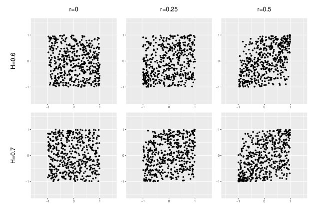
Figure 1: “Linearly” correlated data $(X_{i},Y_{i})$, $i=1,\ldots,500$, with parameters $H$ and $r$.

2. “parabolically” correlated data, i.e. we simulate $k=5000$ repetitions of $(X_{1},\ldots,X_{n},Y_{1}\ldots,Y_{n})$, where $(X_{1},\ldots,X_{n})\mathrel{\hbox to0.0pt{\raisebox{1.29167pt}{$\cdot$}\hss}\raisebox{-1.29167pt}{$\cdot$}}=(2\Phi(Z_{1})-1,\ldots,2\Phi(Z_{n})-1)$, for fractional Gaussian noise $(Z_{i})_{i\geq 1}$ with parameter $H$, and

$$Y_{i}\mathrel{\hbox to0.0pt{\raisebox{1.29167pt}{$\cdot$}\hss}\raisebox{-1.29167pt}{$\cdot$}}=v\left(X_{i}^{2}-\frac{1}{3}\right)+w\xi_{i},\ w=\sqrt{1-\frac{4}{15}v^{2}},$$ (10)

where $(\xi_{i})_{i\geq 1}$ are independent uniformly on $[-1,1]$ distributed random variables; see Figure 2 for an illustration of different parameter combinations. The choice of the parameter $w$ guarantees ${\operatorname{E}}Y_{1}={\operatorname{E}}X_{1}=0$ and ${\operatorname{Var}}\left(Y_{1}\right)={\operatorname{Var}}\left(X_{1}\right)=\frac{1}{3}$.

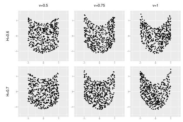
Figure 2: “Parabolically” correlated data $(X_{i},Y_{i})$, $i=1,\ldots,500$, with parameters $H$ and $v$.

3. “wavily” correlated data, i.e. we simulate $k=5000$ repetitions of $(X_{1},\ldots,X_{n},\\ Y_{1}\ldots,Y_{n})$, where $(X_{1},\ldots,X_{n})\mathrel{\hbox to0.0pt{\raisebox{1.29167pt}{$\cdot$}\hss}\raisebox{-1.29167pt}{$\cdot$}}=(2\Phi(Z_{1})-1,\ldots,2\Phi(Z_{n})-1)$, for fractional Gaussian noise $(Z_{i})_{i\geq 1}$ with parameter $H$, and

$$Y_{j}\mathrel{\hbox to0.0pt{\raisebox{1.29167pt}{$\cdot$}\hss}\raisebox{-1.29167pt}{$\cdot$}}=v\left(\left(X_{j}^{2}-\frac{1}{3}\right)^{2}-3/45\right)+w\xi_{j},\ w=\sqrt{1-242/4725v^{2}},$$ (11)

where $(\xi_{i})_{i\geq 1}$ are independent $\mathcal{U}[-1,1]$ distributed random variables; see Figure 3 for an illustration of different parameter combinations. The choice of the parameter $w$ guarantees ${\operatorname{E}}Y_{1}={\operatorname{E}}X_{1}=0$ and ${\operatorname{Var}}\left(Y_{1}\right)={\operatorname{Var}}\left(X_{1}\right)=\frac{1}{3}$.

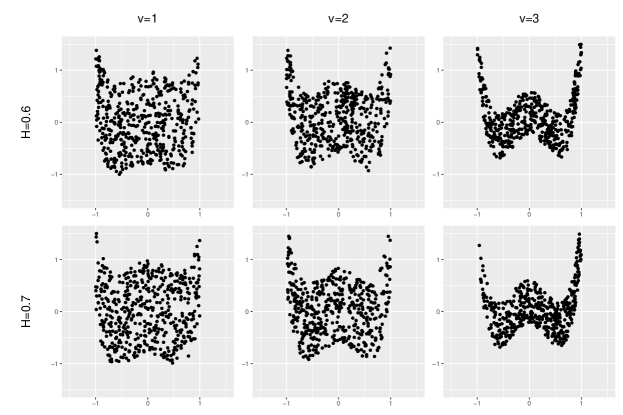
Figure 3: “Wavily” correlated data $(X_{i},Y_{i})$, $i=1,\ldots,500$, with parameters $H$ and $v$.

4. “rectangularly” correlated data, i.e. we simulate $k=5000$ repetitions of $(X_{1},\ldots,X_{n},Y_{1}\ldots,Y_{n})$, where

$$\begin{pmatrix}X_{1}&Y_{1}\\ X_{2}&Y_{2}\\ \vdots&\vdots\\ X_{n}&Y_{n}\end{pmatrix}=\begin{pmatrix}\xi_{1}&\eta_{1}\\ \xi_{2}&\eta_{2}\\ \vdots&\vdots\\ \xi_{n}&\eta_{n}\end{pmatrix}\begin{pmatrix}\cos(\frac{\pi}{12}v)&-\sin(\frac{\pi}{12}v)\\ \sin(\frac{\pi}{12}v)&\cos(\frac{\pi}{12}v)\end{pmatrix}$$ (12)

and for two independent fractional Gaussian noise sequences $(Z_{i})_{i\geq 1}$ and $(\tilde{Z}_{i})_{i\geq 1}$ each with parameter $H$, $(X_{1},\ldots,X_{n})\mathrel{\hbox to0.0pt{\raisebox{1.29167pt}{$\cdot$}\hss}\raisebox{-1.29167pt}{$\cdot$}}=(2\Phi(Z_{1})-1,\ldots,2\Phi(Z_{n})-1)$ and $(Y_{1},\ldots,Y_{n})\mathrel{\hbox to0.0pt{\raisebox{1.29167pt}{$\cdot$}\hss}\raisebox{-1.29167pt}{$\cdot$}}=~{}(2\Phi(\tilde{Z}_{1})-~{}1,\ldots,2\Phi(\tilde{Z}_{n})-1)$; see Figure 4 for an illustration of different parameter combinations.

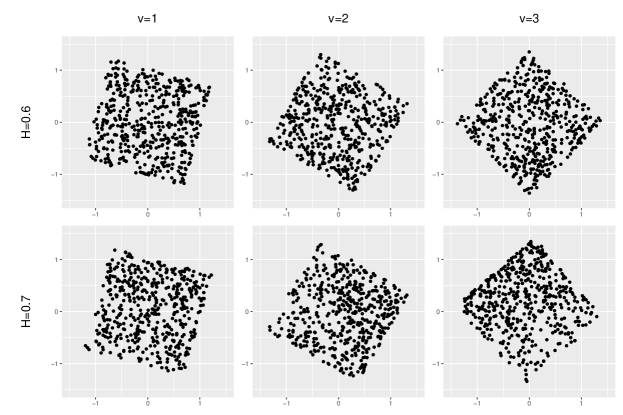
Figure 4: “Rectangularly” correlated data $(X_{i},Y_{i})$, $i=1,\ldots,500$, with parameters $H$ and $v$.

All calculations are based on $5,000$ realizations of simulated time series and test decisions are based on an application of the sampling-window method for a significance level of $5\%$, meaning that the values of the test statistics are compared to the 95%-quantile of the empirical distribution function $\widehat{F}_{m_{n},l_{n}}$ defined by (5). The fractional Gaussian noise sequences are generated by the function simFGN0 from the longmemo package in R. Detailed simulation results can be found in Tables 1 – 4 in the appendix. These display results for sample sizes $n=100,300,500,1000$, block lengths $l_{n}~{}=~{}\lfloor n^{\gamma}\rfloor$ with $\gamma\in\left\{0.4,0.5,0.6\right\}$, Hurst parameters $H=0.6,0.7$ and different values of the parameters $r$ and $v$.

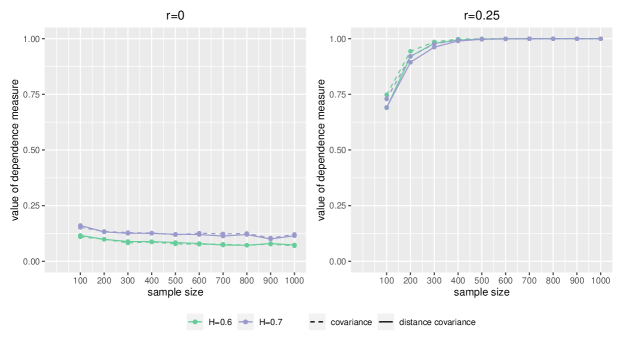
Figure 5: Rejection rates of the hypothesis tests resulting from the empirical covariance and the empirical distance covariance obtained by subsampling based on “linearly” correlated fractional Gaussian noise time series $X_{j}$, $j=1,\ldots,n$, $Y_{j}$, $j=1,\ldots,n$ with block length $l_{n}~{}=~{}\lfloor\sqrt{n}\rfloor$, $d=0.1n$, Hurst parameters $H=0.6,0.7$, and cross-covariance ${\operatorname{Cov}}(X_{i},Y_{j})=r{\operatorname{Cov}}(X_{i},X_{j})$, $1\leq i,j\leq n$, with $r=0$ and $r=0.25$. The level of significance equals 5%.

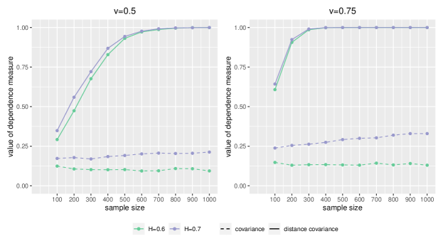
Figure 6: Rejection rates of the hypothesis tests resulting from the empirical covariance and the empirical distance covariance obtained by subsampling based on “parabolically” correlated time series $X_{j}$, $j=~{}1,\ldots,n$, $Y_{j}$, $j=1,\ldots,n$ according to (10) with block length $l_{n}~{}=~{}\lfloor\sqrt{n}\rfloor$, $d=0.1n$, Hurst parameters $H=0.6,0.7$, and with $v=0.5$ and $v=0.75$.

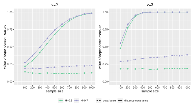
Figure 7: Rejection rates of the hypothesis tests resulting from the empirical covariance and the empirical distance covariance obtained by subsampling based on “wavily” correlated time series $X_{j}$, $j=1,\ldots,n$, $Y_{j}$, $j=1,\ldots,n$ according to (11) with block length $l_{n}~{}=~{}\lfloor\sqrt{n}\rfloor$, $d=0.1n$, Hurst parameters $H=0.6,0.7$, and with $v=2$ and $v=3$. The level of significance equals 5%.

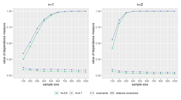
Figure 8: Rejection rates of the hypothesis tests resulting from the empirical covariance and the empirical distance covariance obtained by subsampling based on “rectangularly” correlated time series $X_{j}$, $j=~{}1,\ldots,n$, $Y_{j}$, $j=1,\ldots,n$ according to (12) with block length $l_{n}~{}=~{}\lfloor\sqrt{n}\rfloor$, $d=0.1n$, Hurst parameters $H=0.6,0.7$, and with $v=1$ and $v=2$. The level of significance equals 5%.

As a whole, the simulation results concur with the expected behaviour of hypothesis tests for independence of time series: For both testing procedures, an increasing sample size goes along with an improvement of the finite sample performance of the test, i.e. the empirical size (that can be found in the columns of Table 1 superscribed by $r=0$) approaches the level of significance and the empirical power increases; stronger deviations from the hypothesis, i.e. an increase of the parameters $r$ and $v$ leads to an increase of the rejection rates. Moreover, the testing procedures seem to be sensitive to a dependence within the individual time series, as an increase of the Hurst parameter $H$ results in significantly higher or lower rejection rates.

Both testing procedures tend to be oversized for small sample sizes. Table 1 shows that linear correlation as well as independence of two time series are slightly better detected by a test based on the empirical covariance than by a test based on the empirical distance covariance. For linearly correlated data, an increase of dependence within the time series, i.e. an increase of the parameter $H$, results in a decrease of the empirical power of both testing procedures. For “parabolically” and “wavily” correlated data, this observation can only be made with respect to the finite sample performance of the test based on the empirical distance covariance. Most notably, in these two cases, the test based on the empirical distance covariance clearly outperforms the test based on the empirical covariance in that it yields decisively higher empirical power. In addition to this, it seems remarkable that the test based on the empirical distance covariance interprets a rotation of data points generated by independent stochastic processes as dependence between the coordinates, while the test that is based on the empirical covariance tends to classify these as being generated by independent processes.

4.2 Data example

In the following, the mean monthly discharges of three different rivers are analyzed with regard to cross-dependence between the corresponding data-generating processes by an application of the test statistics considered in the previous sections.

The data was provided by the Global Runoff Data Centre (GRDC) in Koblenz, Germany; see Global Runoff Data Centre (GRDC) . The GRDC is an international archive currently comprising river discharge data of more than 9,900 stations from 159 countries.

The time series we are considering consist of $n=96$ measurements of the mean monthly discharge from January 2000 to December 2007, i.e. a time period of 8 years, for the Amazon River, monitored at a station in São Paulo de Olivença, Brazil (corresponding to GRDC-No. 3623100), the Rhine, monitored at a station in Cologne, Germany (corresponding to GRDC-No. 6335060), and the Jutaí River, a tributary of the Amazon River, monitored at a station in Colocação Caxias (corresponding to GRDC-No. 3624201). (We chose the Jutaí River because its discharge volume compares to that of the Rhine.)

As the discharge volume of rivers is affected by seasonalities and trends, we eliminated these effects from the original data sets by the Small Trend Method, see Brockwell and Davis (1991), Chapter 1.4, p. 21, before our analysis. Figures 9, 10, and 11 depict the values of the detrended and deseasonalized time series.

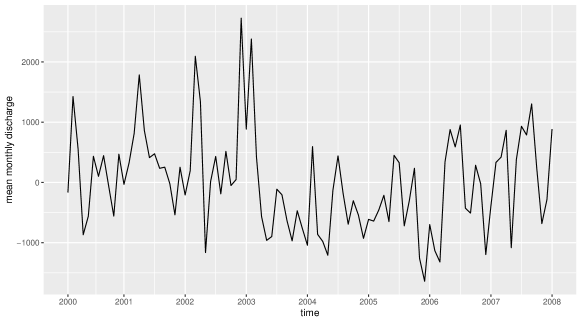
Figure 9: Detrended and deseasonalized mean monthly discharges of the Rhine River.

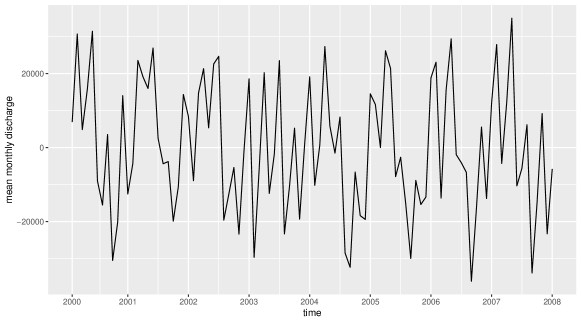
Figure 10: Detrended and deseasonalized mean monthly discharges of the Amazon River.

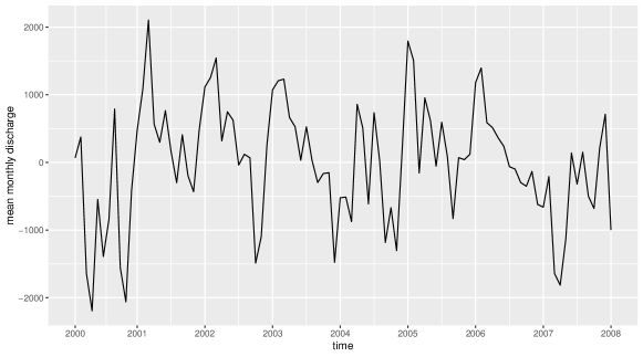
Figure 11: Detrended and deseasonalized mean monthly discharges of the Jutaí River.

The mean monthly discharges of rivers typically display long-range dependence characterized by a Hurst parameter $H$ that is close to $0.7$, meaning the long-range dependence parameter $D$ of the data-generating time series may be assumed to be close to $0.6$. Under a corresponding assumption, a test decision based on the distance cross-covariance rejects the hypothesis for large values of

$$\sqrt{n}\int_{\mathbb{R}^{p}}\int_{\mathbb{R}^{q}}\left|\varphi_{X,Y}^{(n)}(s,t)-\varphi_{X}^{(n)}(s)\varphi_{Y}^{(n)}(t)\right|^{2}s^{-2}t^{-2}dsdt,$$

while a test decision based on the empirical cross-covariance rejects the hypothesis for large values of

$$\frac{1}{\sqrt{n}}\left|\sum\limits_{i=1}^{n}(X_{i}-\bar{X})(Y_{i}-\bar{Y})\right|.$$

In our analysis, we apply both tests to the data. We base test decisions on an approximation of the distribution of the test statistics by the sampling-window method with block size $l=~{}\lfloor\sqrt{n}\rfloor=9$. As significance level we choose $\alpha=5\%$.

As the Rhine is geographically separated from the other two rivers, we expect the tests to decide in favor of the hypothesis of independence, when applied to the discharges of the Rhine and one of the Brazilian rivers. Due to the fact that the Jutaí River is a tributary of the Amazon River, and due to the spatial proximity of the two measuring stations in Brazil, which are approximately 200 kilometers apart, we expect a test for independence of the discharge volumes of these two rivers to reject the hypothesis. In fact, both tests do not reject the hypothesis of two independent time series when applied to the Rhine’s discharge and the Amazon River’s or Jutaí River’s discharge, respectively, and reject the hypothesis when applied to the discharges of the two Brazilian rivers.

Appendix A Gaussian subordination and Long-range dependence

This article focuses on the consideration of subordinated Gaussian time series, i.e. on random observations generated by transformations of Gaussian processes.

Definition A.1.

Let $(\xi_{t})_{t\in T}$ be a Gaussian process with index set $T$. A process $(Y_{t})_{t\in~{}T}$ satisfying $Y_{t}=G(\xi_{t})$ for some measurable function $G:\mathbb{R}\longrightarrow\mathbb{R}$ is called subordinated Gaussian process.

Remark A.1.

For any particular distribution function $F$, an appropriate choice of the transformation $G$ in Definition A.1 yields subordinated Gaussian processes with marginal distribution $F$. Moreover, there exist algorithms for generating Gaussian processes that, after suitable transformation, yield subordinated Gaussian processes with marginal distribution $F$ and a predefined covariance structure; see Pipiras and Taqqu (2017).

Univariate Hermite expansion

The subordinated random variables $Y_{t}=G(\xi_{t})$, $t\in~{}T$, can be considered as elements of the Hilbert space $L^{2}(\mathbb{R},\varphi(x)dx)=~{}\mathcal{L}^{2}(\mathbb{R},\varphi(x)dx)/\mathcal{N}$, where $\mathcal{L}^{2}(\mathbb{R},\varphi(x)dx)$ denotes the space of all measurable, real-valued functions which are square-integrable with respect to the measure $\varphi(x)dx$ associated with the standard normal density function $\varphi$ and $\mathcal{N}\mathrel{\hbox to0.0pt{\raisebox{1.29167pt}{$\cdot$}\hss}\raisebox{-1.29167pt}{$\cdot$}}=~{}\text{ker}(\|\cdot\|_{L^{2}})$. For two functions $G_{1},G_{2}\in L^{2}(\mathbb{R},\varphi(x)dx)$ the corresponding inner product is defined by

$$\langle G_{1},G_{2}\rangle_{L^{2}}\mathrel{\hbox to0.0pt{\raisebox{1.29167pt}{$\cdot$}\hss}\raisebox{-1.29167pt}{$\cdot$}}=\displaystyle\int_{-\infty}^{\infty}G_{1}(x)G_{2}(x)\varphi(x)dx={\operatorname{E}}G_{1}(X)G_{2}(X)$$ (13)

with $X$ denoting a standard normally distributed random variable.

A collection of orthogonal elements in $L^{2}(\mathbb{R},\varphi(x)dx)$ is given by the sequence of Hermite polynomials; see Pipiras and Taqqu (2017).

Definition A.2.

For $n\geq 0$, the Hermite polynomial of order $n$ is defined by

$$H_{n}(x)=(-1)^{n}{\operatorname{e}}^{\frac{1}{2}x^{2}}\frac{d^{n}}{dx^{n}}{\operatorname{e}}^{-\frac{1}{2}x^{2}},\ x\in\mathbb{R}.$$

Orthogonality of the sequence $(H_{n})_{n\geq 0}$ in $L^{2}(\mathbb{R},\varphi(x)dx)$ follows from

$$\langle H_{n},H_{m}\rangle_{L^{2}}=\begin{cases}n!\ \ &\text{if $n=m$,}\\ 0\ \ &\text{if $n\neq m$.}\end{cases}$$

Moreover, it can be shown that the Hermite polynomials form an orthogonal basis of $L^{2}(\mathbb{R},\varphi(x)dx)$. As a result, every $G\in L^{2}(\mathbb{R},\varphi(x)dx)$ has an expansion in Hermite polynomials, i.e. for $G\in L^{2}(\mathbb{R},\varphi(x)dx)$ and $\xi$ standard normally distributed, we have

$$G(\xi)=\sum\limits_{r=0}^{\infty}\frac{J_{r}(G)}{r!}H_{r}(\xi),$$ (14)

where the so-called Hermite coefficient $J_{r}(G)$ is given by

$$J_{r}(G):=\langle G,H_{r}\rangle_{L^{2}}={\operatorname{E}}G(X)H_{r}(X).$$

Equation (14) holds in an $L^{2}$-sense, meaning

$$\lim\limits_{n\rightarrow\infty}\left\|G(\xi)-\sum\limits_{r=0}^{n}\frac{J_{r}(G)}{r!}H_{r}(\xi)\right\|_{L^{2}}=0,$$

where $\|\cdot\|_{L^{2}}$ denotes the norm induced by the inner product $\langle\cdot,\cdot\rangle_{L^{2}}$.

Given the Hermite expansion (14), it is possible to characterize the dependence structure of subordinated Gaussian time series $G(\xi_{n})$, $n\in\mathbb{N}$. In fact, it holds that

$${\operatorname{Cov}}(G(\xi_{1}),G(\xi_{k+1}))=\sum\limits_{r=1}^{\infty}\frac{J^{2}_{r}(G)}{r!}\left(\rho(k)\right)^{r},$$ (15)

where $\rho$ denotes the auto-covariance function of $(\xi_{n})_{n\geq 1}$; see Pipiras and Taqqu (2017). Under the assumption that, as $k$ tends to $\infty$, $\rho(k)$ converges to $0$ with a certain rate, the asymptotically dominating term in the series (15) is the summand corresponding to the smallest integer $r$ for which the Hermite coefficient $J_{r}(G)$ is non-zero. This index, which decisively depends on $G$, is called Hermite rank.

Definition A.3.

Let $G\in L^{2}(\mathbb{R},\varphi(x)dx)$ with ${\operatorname{E}}G(X)=0$ for standard normally distributed $X$ and let $J_{r}(G)$, $r\geq 0$, be the Hermite coefficients in the Hermite expansion of $G$. The smallest index $k\geq 1$ for which $J_{k}(G)\neq 0$ is called the Hermite rank of $G$, i.e.

$$r\mathrel{\hbox to0.0pt{\raisebox{1.29167pt}{$\cdot$}\hss}\raisebox{-1.29167pt}{$\cdot$}}=\min\left\{k\geq 1:J_{k}(G)\neq 0\right\}.$$

Multivariate Hermite expansion

Let $(\xi_{t})_{t\in T}$, be a multivariate Gaussian process with index set $T$. More precisely, assume that $\xi_{t}\mathrel{\hbox to0.0pt{\raisebox{1.29167pt}{$\cdot$}\hss}\raisebox{-1.29167pt}{$\cdot$}}=(\xi^{(1)}_{t},\xi^{(2)}_{t},\ldots,\xi^{(d)}_{t})$ are Gaussian random vectors with mean $\mathbf{0}\mathrel{\hbox to0.0pt{\raisebox{1.29167pt}{$\cdot$}\hss}\raisebox{-1.29167pt}{$\cdot$}}=(0,\ldots,0)^{\top}$ and covariance matrix $\Sigma$. We write $\varphi_{\Sigma}$ for the corresponding density and denote by $I_{d}$ the $d\times d$ identity matrix. Set $\mathbf{q}=(q_{1},\ldots,q_{d})^{\top}$, $\mathbf{q}=q_{1}!\cdots q_{d}!$, $|\mathbf{q}|=q_{1}+\ldots+q_{d}$, $\mathbf{x}=(x_{1},\ldots,x_{d})^{\top}$, $\mathbf{x}^{\mathbf{q}}=x_{1}^{q_{1}}\cdots x_{d}^{q_{d}}$, $\partial\mathbf{x}^{\mathbf{q}}=\partial x_{1}^{q_{1}}\cdots\partial x_{d}^{q_{d}}$ and

$$\left(\frac{d}{d\mathbf{x}}\right)^{\mathbf{q}}=\frac{\partial^{|\mathbf{q}|}}{\partial\mathbf{x}^{\mathbf{q}}}=\frac{\partial^{q_{1}+\ldots+q_{d}}}{\partial x_{1}^{q_{1}}\cdots\partial x_{d}^{q_{d}}}.$$

Given a measurable function $G:\mathbb{R}^{d}\longrightarrow\mathbb{R}$, subordinated random variables $Y=G(\xi_{t})$, $t\in T$, can be considered as elements of the Hilbert space $L^{2}(\mathbb{R}^{d},\varphi_{\Sigma})=\mathcal{L}^{2}(\mathbb{R}^{d},\varphi_{\Sigma})/\mathcal{N}$, where $\mathcal{L}^{2}(\mathbb{R}^{d},\varphi_{\Sigma})$ denotes the space of all measurable, real-valued functions which are square-integrable with respect to the measure associated with the density function $\varphi_{\Sigma}$ and $\mathcal{N}\mathrel{\hbox to0.0pt{\raisebox{1.29167pt}{$\cdot$}\hss}\raisebox{-1.29167pt}{$\cdot$}}=~{}\text{ker}(\|\cdot\|_{L^{2}})$. For two functions $G_{1},G_{2}\in L^{2}(\mathbb{R}^{d},\varphi_{I_{2}})$ the corresponding inner product is defined by

$$\langle G_{1},G_{2}\rangle_{L^{2}}\mathrel{\hbox to0.0pt{\raisebox{1.29167pt}{$\cdot$}\hss}\raisebox{-1.29167pt}{$\cdot$}}=\displaystyle\int_{-\infty}^{\infty}G_{1}(x)G_{2}(x)\varphi_{I_{d}}(x)dx={\operatorname{E}}G_{1}(\mathbf{X})G_{2}(\mathbf{X})$$ (16)

with $\mathbf{X}$ denoting a standard normally distributed, $d$-variate random vector.

Definition A.4.

For $\mathbf{x}=(x_{1},\ldots,x_{d})^{\top}\in\mathbb{R}^{d}$ and $\mathbf{q}=(q_{1},\ldots,q_{k})^{\top}\in\mathbb{N}^{d}$ we call $H_{\mathbf{q}}$, defined by

$$H_{\mathbf{q}}(\mathbf{x};\Sigma)\mathrel{\hbox to0.0pt{\raisebox{1.29167pt}{$\cdot$}\hss}\raisebox{-1.29167pt}{$\cdot$}}=\frac{(-1)^{|\mathbf{q}|}}{\varphi_{\Sigma}(\mathbf{x})}\left(\frac{d}{d\mathbf{x}}\right)^{q}\varphi_{\Sigma}(\mathbf{x}),$$

a multivariate Hermite polynomial of degree $k=|\mathbf{q}|$.

If $\Sigma=I_{d}$ then $H_{\mathbf{q}}(\mathbf{x};\Sigma)=\prod_{j=1}^{d}H_{q_{j}}(x_{j})$, i.e. if the components of the vector $\mathbf{X}$ are independent, then a multivariate Hermite polynomial is a product of univariate ones. In the following it is shown that, in fact, it is sufficient to consider Gaussian random vectors with independent, identically distributed components, i.e.

$$\tilde{\mathbf{X}}=(\tilde{X}_{1},\ldots,\tilde{X}_{d})^{\top}\sim\mathcal{N}(0,I_{d}).$$

Let $G\in L^{2}(\mathbb{R}^{d},\varphi_{I_{d}})$ and define

$$J(G,\tilde{\mathbf{X}},\mathbf{q})=J(G,I_{d},\mathbf{q})=\langle G,H^{*}_{\mathbf{q}}\rangle={\operatorname{E}}\left(G(\tilde{\mathbf{X}})H^{*}_{\mathbf{q}}(\tilde{\mathbf{X}})\right),$$

where

$$H^{*}_{\mathbf{q}}(\mathbf{x})=H^{*}_{q_{1},\ldots,q_{k}}(x_{1},\ldots,x_{d})=\prod\limits_{j=1}^{d}H_{q_{j}}(x_{j}).$$

The Hermite rank $r(G,\tilde{\mathbf{X}})=r(G,I_{d})$ of $G$ with respect to $\tilde{\mathbf{X}}$, i.e. with respect to the distribution $\mathcal{N}(0,I_{d})$, is the largest integer $r$ such that $J(G,I_{d},\mathbf{q})=0$ for all $0<|\mathbf{q}|<r$, where $|\mathbf{q}|=q_{1}+\ldots+q_{d}$. Note that this is the same as the largest integer $r$ such that

$$\langle G(\tilde{\mathbf{X}}),\tilde{\mathbf{X}}^{\mathbf{q}}\rangle={\operatorname{E}}\left(G(\tilde{\mathbf{X}})\prod\limits_{j=1}^{d}\tilde{X}_{j}^{q_{j}}\right)=0\ \text{for all}\ 0<|\mathbf{q}|<r.$$

As in the univariate case, we have the orthogonal expansion

$$G(\tilde{X}_{1},\ldots,\tilde{X}_{d})={\operatorname{E}}(G(\tilde{\mathbf{X}}))+\sum\limits_{|\mathbf{q}|\geq r(G,I_{d})}\frac{J(G,I_{d},\mathbf{q})}{q_{1}!\cdots q_{d}!}\prod\limits_{j=1}^{d}H_{q_{j}}(\tilde{X}_{j}).$$

Since $\mathbf{X}\sim\mathcal{N}(0,\Sigma)$ is equal in distribution to $U(\tilde{\mathbf{X}})=\Sigma^{\frac{1}{2}}\tilde{\mathbf{X}}$, we have the expansion

$$G(\mathbf{X})=\tilde{G}(\tilde{\mathbf{X}})={\operatorname{E}}(G(\mathbf{X})+\sum\limits_{|\mathbf{q}|\geq r(\tilde{G},I_{d})}\frac{J(G\circ U,I_{d},\mathbf{q})}{q_{1}!\cdots q_{d}!}\prod\limits_{j=1}^{d}H_{q_{j}}(\tilde{X}_{j}).$$

Definition A.5.

Let $\mathbf{X}\sim\mathcal{N}(0,\Sigma)$ and $G\in L^{2}(\mathbb{R}^{d},\varphi_{I_{d}})$. We define the Hermite coefficients of $G$ with respect to $\mathbf{X}$ by

$$J(G,\mathbf{X},\mathbf{q})=J(G,\Sigma,\mathbf{q})={\operatorname{E}}\left(G(\mathbf{X})H_{\mathbf{q}}^{*}(\mathbf{X})\right).$$

The Hermite rank $r(G,\mathbf{X})=r(G,\Sigma)$ is defined as the largest integer $r$ such that

$$J(G,\Sigma,\mathbf{q})=0\ \text{for all}\ 0<|\mathbf{q}|<r.$$

Remark A.2.

It follows that

$$r(G,\Sigma)=r(G\circ U,I_{d}).$$

Long-range dependence

In this article, we study the asymptotic behavior of distance covariance for long-range dependent time series. The rate of decay of the auto-covariance function is crucial to the definition of long-range dependent time series. A relatively slow decay of the auto-covariances characterizes long-range dependent time series, while a relatively fast decay characterizes short-range dependent processes; see Pipiras and Taqqu (2017), p. 17.

Definition A.6.

A (second-order) stationary, real-valued time series $(X_{k})_{k\geq 1}$, is called long-range dependent if its auto-covariance function $\rho$ satisfies

$$\rho(k)\mathrel{\hbox to0.0pt{\raisebox{1.29167pt}{$\cdot$}\hss}\raisebox{-1.29167pt}{$\cdot$}}={\operatorname{Cov}}(X_{1},X_{k+1})\sim k^{-D}L(k),\ \ \text{as $k\rightarrow\infty$,}$$

with $D\in\left(0,1\right)$ for some slowly varying function $L$. We refer to $D$ as long-range dependence (LRD) parameter.

It follows from (15) that subordination of long-range dependent Gaussian time series potentially generates time series whose auto-covariances decay faster than the auto-covariances of the underlying Gaussian process. In some cases, the subordinated time series is long-range dependent as well, in other cases subordination may even yield short-range dependence. Given that ${\operatorname{Cov}}(\xi_{1},\xi_{k+1})\sim k^{-D}L(k)$, as $k\rightarrow\infty$, for some slowly varying function $L$ and $D\in(0,1)$ and given that $G\in L^{2}(\mathbb{R},\varphi(x)dx)$ is a function with Hermite rank $r$, we have

$${\operatorname{Cov}}(G(\xi_{1}),G(\xi_{k+1}))\sim J_{r}^{2}(G)r!k^{-Dr}L^{r}(k),\ \ \text{as $k\rightarrow\infty$.}$$

It immediately follows that subordinated Gaussian time series $G(\xi_{n})$, $n\geq 1$, are long-range dependent with LRD parameter $D_{G}\mathrel{\hbox to0.0pt{\raisebox{1.29167pt}{$\cdot$}\hss}\raisebox{-1.29167pt}{$\cdot$}}=Dr$ and slowly-varying function $L_{G}(k)=~{}J_{r}^{2}(G)r!L^{r}(k)$ whenever $Dr<1$.

Appendix B Proofs

Proof of Lemma 2.1.

Define $u_{j}(s)\mathrel{\hbox to0.0pt{\raisebox{1.29167pt}{$\cdot$}\hss}\raisebox{-1.29167pt}{$\cdot$}}=\exp(isX_{j})-\varphi_{X}(s)$. Then, it follows that

$$\varphi_{X}^{(n)}(s)-\varphi_{X}(s)=\frac{1}{n}\sum\limits_{j=1}^{n}u_{j}(s).$$

In order to show that $\varphi_{X}^{(n)}(s)-\varphi_{X}(s)$ is an element of the vector space $L^{2}(\mathbb{R},\omega(s)ds)$, it thus suffices to show that $u_{j}\in L^{2}(\mathbb{R},\omega(s)ds)$. For this, note that

$$|u_{j}(s)|^{2} =\left(\exp(isX_{j})-{\operatorname{E}}\left(\exp(isX_{j})\right)\right)\left(\exp(-isX_{j})-{\operatorname{E}}\left(-\exp(isX_{j})\right)\right)$$

$$=1+\varphi_{X}(s)\bar{\varphi}_{X}(s)-\exp(isX_{j})\bar{\varphi}_{X}(s)-\exp(-isX_{j})\varphi_{X}(s).$$

For $X^{\prime}\overset{\mathcal{D}}{=}X$, independent of $X$, and ${\operatorname{E}}_{X}$ denoting the expected value taken with respect to $X$, we have

$$\varphi_{X}(s)\bar{\varphi}_{X}(s) ={\operatorname{E}}\left[\left(\cos(sX)+i\sin(sX)\right)\left(\cos(sX^{\prime})-i\sin(sX^{\prime})\right)\right]$$

$$={\operatorname{E}}\left[\cos(sX)\cos(sX^{\prime})+\sin(sX)\sin(sX^{\prime})\right]$$

$$={\operatorname{E}}\left[\cos(s(X-X^{\prime}))\right],$$

$$\exp(isX_{j})\bar{\varphi}_{X}(s)$$

$$= \left(\cos(sX_{j})+i\sin(sX_{j})\right){\operatorname{E}}\left(\cos(sX)-i\sin(sX)\right)$$

$$= {\operatorname{E}}_{X}\left(\cos(sX_{j})\cos(sX)+\sin(sX)\sin(sX_{j})\right)$$

$$+i\sin(sX_{j}){\operatorname{E}}\left(\cos(sX)\right)-i\cos(sX_{j}){\operatorname{E}}\left(\sin(sX)\right)$$

$$= {\operatorname{E}}_{X}\left(\cos(s(X_{j}-X))\right)+i\sin(sX_{j}){\operatorname{E}}\left(\cos(sX)\right)-i\cos(sX_{j}){\operatorname{E}}\left(\sin(sX)\right),$$

and

$$\exp(-isX_{j})\varphi_{X}(s)$$

$$= \left(\cos(sX_{j})-i\sin(sX_{j})\right){\operatorname{E}}\left(\cos(sX)+i\sin(sX)\right)$$

$$= {\operatorname{E}}_{X}\left(\cos(sX_{j})\cos(sX)+\sin(sX)\sin(sX_{j})\right)$$

$$-i\sin(sX_{j}){\operatorname{E}}\left(\cos(sX)\right)+i\cos(sX_{j}){\operatorname{E}}\left(\sin(sX)\right)$$

$$= {\operatorname{E}}_{X}\left(\cos(s(X_{j}-X))\right)-i\sin(sX_{j}){\operatorname{E}}\left(\cos(sX)\right)+i\cos(sX_{j}){\operatorname{E}}\left(\sin(sX)\right).$$

It follows that

$$|u_{j}(s)|^{2}=2{\operatorname{E}}_{X}\left[1-\cos(s(X_{j}-X))\right]-{\operatorname{E}}\left[1-\cos(s(X-X^{\prime}))\right].$$

As a result, and according to Lemma 1 in Székely, Rizzo and Bakirov (2007), we arrive at

$$\int_{\mathbb{R}}\frac{|u_{j}(s)|^{2}}{|s|^{2}}ds$$

$$= \int_{\mathbb{R}}\frac{1}{|s|^{2}}\left(2{\operatorname{E}}_{X}\left[1-\cos(s(X_{j}-X))\right]-{\operatorname{E}}\left[1-\cos(s(X-X^{\prime}))\right]\right)ds$$

$$= \left(2{\operatorname{E}}_{X}\left[\int_{\mathbb{R}}\frac{1}{|s|^{2}}\left(1-\cos(s(X_{j}-X))\right)ds\right]-{\operatorname{E}}\left[\int_{\mathbb{R}}\frac{1}{|s|^{2}}\left(1-\cos(s(X-X^{\prime}))\right)ds\right]\right)$$

$$= 2\left({\operatorname{E}}_{X}(|X_{j}-X|)-{\operatorname{E}}|X-X^{\prime}|\right)\leq 2\left(|X_{j}|+{\operatorname{E}}|X|\right).$$

Consequently, $\varphi_{X}^{(n)}(s)-\varphi_{X}(s)$ takes values in $L^{2}\left(\mathbb{R},\omega(s)ds\right)$.

Furthermore, it holds that

$$\int_{\mathbb{R}}\int_{\mathbb{R}}\left|\left(\varphi_{Y}^{(n)}(t)-\varphi_{Y}(t)\right)\left(\varphi_{X}^{(n)}(s)-\varphi_{X}(s)\right)\right|^{2}\omega(s,t)dsdt\\ =\int_{\mathbb{R}}\left|\varphi_{X}^{(n)}(s)-\varphi_{X}(s)\right|^{2}(cs^{2})^{-1}ds\int_{\mathbb{R}}\left|\varphi_{Y}^{(n)}(t)-\varphi_{Y}(t)\right|^{2}(ct^{2})^{-1}dt<\infty,$$

i.e. $\left(\varphi_{Y}^{(n)}(t)-\varphi_{Y}(t)\right)\left(\varphi_{X}^{(n)}(s)-\varphi_{X}(s)\right)$ takes values in $L^{2}\left(\mathbb{R}^{2},\omega(s,t)dsdt\right)$. ∎

Proof of Theorem 2.2.

In order to show convergence of the test statistic we apply Theorem 4.2 in Billingsley (1968). For this, we define

$$V_{n}\mathrel{\hbox to0.0pt{\raisebox{1.29167pt}{$\cdot$}\hss}\raisebox{-1.29167pt}{$\cdot$}}=\sum\limits_{h=0}^{\infty}a_{h}{\mathcal{V}}_{n}^{2}(X,Y;h),\ \ V\mathrel{\hbox to0.0pt{\raisebox{1.29167pt}{$\cdot$}\hss}\raisebox{-1.29167pt}{$\cdot$}}=Z\sum\limits_{h=0}^{\infty}a_{h},$$

$$U_{m,n}\mathrel{\hbox to0.0pt{\raisebox{1.29167pt}{$\cdot$}\hss}\raisebox{-1.29167pt}{$\cdot$}}=\sum\limits_{h=0}^{m}a_{h}{\mathcal{V}}_{n}^{2}(X,Y;h),\ \ U_{m}\mathrel{\hbox to0.0pt{\raisebox{1.29167pt}{$\cdot$}\hss}\raisebox{-1.29167pt}{$\cdot$}}=Z\sum\limits_{h=0}^{m}a_{h}.$$

Based on Proposition 3.4 it follows from an application of the continuous mapping theorem that $U_{m,n}\overset{\mathcal{D}}{\longrightarrow}U_{m}$, $n\rightarrow\infty$.

Moreover, we have

$${\operatorname{E}}\left|U_{m}-V\right|\leq{\operatorname{E}}\left|Z\right|\sum\limits_{h=m+1}^{\infty}\left|a_{h}\right|.$$

The right-hand side of the above inequality goes to $0$ since, by assumption, $\lim_{m\rightarrow\infty}\sum_{h=m+1}^{\infty}|a_{h}|=0$. Consequently, $U_{m}\overset{\mathcal{D}}{\longrightarrow}V$, $m\rightarrow\infty$.

For any $\epsilon>0$ it holds that

$$P\left(\left|U_{m,n}-V_{n}\right|\geq\epsilon\right)\leq\frac{1}{\epsilon}{\operatorname{E}}\left|U_{m,n}-V_{n}\right|\leq{\operatorname{E}}\left|{\mathcal{V}}_{n}^{2}(X,Y;0)\right|\sum\limits_{h=m+1}^{\infty}|a_{h}|.$$

Since for some constant $C$, ${\operatorname{E}}\left(\left|\int_{{\mathbb{R}}^{p}}\int_{{\mathbb{R}}^{q}}\big{|}Z_{n}(s,t;0)\big{|}^{2}w(s,t)ds\,dt\right|\right)\leq C$ for all $n\in\mathbb{N}$, and since $\lim_{m\rightarrow\infty}\sum_{h=m+1}^{\infty}|a_{h}|=0$ by assumption, it follows that

$$\lim\limits_{m\rightarrow\infty}\limsup\limits_{n\rightarrow\infty}P\left(\left|U_{m,n}-V_{n}\right|\geq\epsilon\right)=0.$$

Theorem 4.2 in Billingsley (1968) therefore yields $V_{n}\overset{\mathcal{D}}{\longrightarrow}V$. ∎

Proof of Theorem 2.3.

In order to establish the validity of the subsampling procedure, note that the triangular inequality yields

$$|\widehat{F}_{m_{n},l_{n}}(t)-F_{T_{n}}(t)|\leq|\widehat{F}_{m_{n},l_{n}}(t)-F_{T}(t)|+|F_{T}(t)-F_{T_{n}}(t)|.$$ (17)

The second term on the right-hand side of the inequality converges to $0$ for all points of continuity $t$ of $F_{T}$ if the statistics $T_{n}$, $n\in\mathbb{N}$, are measurable and converge in distribution to a (non-degenerate) random variable $T$ with distribution function $F_{T}$.

It remains to show that the first summand on the right-hand side of inequality (17) converges to $0$ as well. As $L^{2}$-convergence implies convergence in probability, it suffices to show that $\lim_{n\rightarrow\infty}{\operatorname{E}}|\widehat{F}_{m_{n},l_{n}}(t)-F_{T}(t)|^{2}=0$. For this purpose, we consider the following bias-variance decomposition:

$${\operatorname{E}}\left(|\widehat{F}_{m_{n},l_{n}}(t)-F_{T}(t)|^{2}\right)={\operatorname{Var}}\left(\widehat{F}_{m_{n},l_{n}}(t)\right)+\left|{\operatorname{E}}\widehat{F}_{m_{n},l_{n}}(t)-F_{T}(t)\right|^{2}.$$

Stationarity and independence of the processes $(X_{n})_{n\geq 1}$ and $(Y_{n})_{n\geq 1}$ imply that ${\operatorname{E}}\widehat{F}_{m_{n},l_{n}}(t)=F_{T_{l}}(t)$, so that, due to the convergence of $T_{n}$, the bias term of the above equation converges to $0$ as $l_{n}$ tends to $\infty$.

As a result, it remains to show that the variance term vanishes as $n$ tends to $\infty$. Initially, note that

$${\operatorname{Var}}\left(\widehat{F}_{m_{n},l_{n}}(t)\right)$$

$$= \frac{1}{m_{n}}{\operatorname{Var}}\left(1_{\left\{T_{l_{n},1}\leq t\right\}}\right)+\frac{2}{m_{n}^{2}}\sum\limits_{k=2}^{m_{n}}(m_{n}-i+1){\operatorname{Cov}}\left(1_{\left\{T_{l_{n},1}\leq t\right\}},1_{\left\{T_{l_{n},k}\leq t\right\}}\right)$$

$$\leq \frac{2}{m_{n}}\sum\limits_{k=1}^{m_{n}}\left|{\operatorname{Cov}}\left(1_{\left\{T_{l_{n},1}\leq t\right\}},1_{\left\{T_{l_{n},k}\leq t\right\}}\right)\right|$$

due to stationarity.

Since $T_{l_{n},k}=T_{l_{n}}\left(X_{k},\ldots,X_{k+l_{n}-1},Y_{k+d_{n}},\ldots,Y_{k+d_{n}+l_{n}-1}\right)$,

$$\left|{\operatorname{Cov}}\left(1_{\left\{T_{l_{n},1}\leq t\right\}},1_{\left\{T_{l_{n},k}\leq t\right\}}\right)\right|$$

$$\leq\rho\left(\sigma(X_{i},Y_{d_{n}+i},1\leq i\leq l_{n}),\sigma(X_{j},Y_{d_{n}+j},k\leq j\leq k+l_{n}-1)\right),$$

where $\sigma(X_{i},Y_{d_{n}+i},1\leq i\leq l_{n})$ and $\sigma(X_{j},Y_{d_{n}+j},k\leq j\leq k+l_{n}-1)$) denote the $\sigma$-fields generated by the random variables $X_{i},Y_{d_{n}+i},1\leq i\leq l_{n}$, and $X_{j},Y_{d_{n}+j},k\leq j\leq k+l_{n}-1$), respectively.

For $\beta\in(0,1)$, we split the sum of covariances into two parts:

$$\frac{1}{m_{n}}\sum\limits_{k=1}^{m_{n}}\left|{\operatorname{Cov}}\left(1_{\left\{T_{l_{n},1}\leq t\right\}},1_{\left\{T_{l_{n},k}\leq t\right\}}\right)\right|$$

$$= \frac{1}{m_{n}}\sum\limits_{k=1}^{\lfloor n^{\beta}\rfloor}\!\!\left|{\operatorname{Cov}}\left(1_{\left\{T_{l_{n},1}\leq t\right\}},1_{\left\{T_{l_{n},k}\leq t\right\}}\right)\right|+\frac{1}{m_{n}}\sum\limits_{k=\lfloor n^{\beta}\rfloor+1}^{m_{n}}\!\!\!\!\left|{\operatorname{Cov}}\left(1_{\left\{T_{l_{n},1}\leq t\right\}},1_{\left\{T_{l_{n},k}\leq t\right\}}\right)\right|$$

$$\leq \frac{\lfloor n^{\beta}\rfloor}{m_{n}}+\frac{1}{m_{n}}\sum\limits_{k=\lfloor n^{\beta}\rfloor+1}^{m_{n}}\rho\left(\sigma(X_{i},Y_{d_{n}+i},1\leq i\leq l_{n}),\sigma(X_{j},Y_{d_{n}+j},k\leq j\leq k+l_{n}-1)\right)$$

$$\leq \frac{\lfloor n^{\beta}\rfloor}{m_{n}}+\frac{1}{m_{n}}\sum\limits_{k=\lfloor n^{\beta}\rfloor+1}^{m_{n}}\rho_{k,l_{n},d_{n}},$$

where

$$\rho_{k,l_{n},d_{n}}\mathrel{\hbox to0.0pt{\raisebox{1.29167pt}{$\cdot$}\hss}\raisebox{-1.29167pt}{$\cdot$}}=\rho\left(\sigma(X_{i},Y_{d_{n}+i},1\leq i\leq l_{n}),\sigma(X_{j},Y_{d_{n}+j},k\leq j\leq k+l_{n}-1)\right).$$

The first summand on the right-hand side of the inequality converges to $0$ if $l_{n}=o(n)$ and $d_{n}=o(n)$. In order to show that the second summand converges to $0$, a sufficiently good approximation to the sum of maximal correlations is needed. In particular, we have to show that

$$\sum\limits_{k=\lfloor n^{\beta}\rfloor+1}^{m_{n}}\rho_{k,l_{n},d_{n}}=o(m_{n}).$$

According to Bradley (2005), Theorem 5.1,

$$\rho(\mathcal{A}_{1}\vee\mathcal{A}_{2},\mathcal{B}_{1}\vee\mathcal{B}_{2})\leq\max\left\{\rho(\mathcal{A}_{1},\mathcal{B}_{1}),\rho(\mathcal{A}_{2},\mathcal{B}_{2})\right\},$$

if $\mathcal{A}_{1}\vee\mathcal{B}_{1}$ and $\mathcal{A}_{2}\vee\mathcal{B}_{2}$ are independent.

As a result (and because of stationarity), it holds that

$$\rho_{k,l_{n},d_{n}}\leq\max\{\rho_{k,l_{n},X},\rho_{k,l_{n},Y}\},$$

where

$$\rho_{k,l_{n},X}\mathrel{\hbox to0.0pt{\raisebox{1.29167pt}{$\cdot$}\hss}\raisebox{-1.29167pt}{$\cdot$}}= \rho\left(\sigma(X_{i},1\leq i\leq l_{n}),\sigma(X_{j},k\leq j\leq k+l_{n}-1)\right),$$

$$\rho_{k,l_{n},Y}\mathrel{\hbox to0.0pt{\raisebox{1.29167pt}{$\cdot$}\hss}\raisebox{-1.29167pt}{$\cdot$}}= \rho\left(\sigma(Y_{i},1\leq i\leq l_{n}),\sigma(Y_{j},k\leq j\leq k+l_{n}-1)\right).$$

For this reason, it suffices to show that

$$\sum\limits_{k=\lfloor n^{\beta}\rfloor+1}^{m_{n}}\rho_{k,l_{n},X}=\sum\limits_{k=\lfloor n^{\beta}\rfloor+1}^{m_{n}}\rho_{k,l_{n},Y}=o(m_{n}).$$

Betken and Wendler (2018) establish the following result:

Lemma B.1 (Betken and Wendler (2018)).

Given a time series $\xi_{k}$, $k\geq 1$, satisfying Assumptions 1 and 2, there exist constants $C_{1},C_{2}\in(0,\infty)$, such that

$$\rho\left(\sigma(\xi_{i},1\leq i\leq l),\sigma(\xi_{j},k+l\leq j\leq k+2l-1)\right)\\ \leq C_{1}l^{D}k^{-D}L_{\rho}(k)+C_{2}l^{2}k^{-D-1}\max\{L_{\rho}(k),1\}$$

for all $k\in\mathbb{N}$ and all $l\in\{l_{k},\ldots,k\}$.

We consider $\sum_{k=\lfloor n^{\beta}\rfloor+1}^{m_{n}}\rho_{k,l_{n},X}$ only, since the same argument yields

$$\sum\limits_{k=\lfloor n^{\beta}\rfloor+1}^{m_{n}}\rho_{k,l_{n},Y}=~{}o(m_{n}).$$

Let $\varepsilon>0$. By assumption, $l_{n}\leq C_{l}n^{\alpha}$ for $\alpha\mathrel{\hbox to0.0pt{\raisebox{1.29167pt}{$\cdot$}\hss}\raisebox{-1.29167pt}{$\cdot$}}=\frac{1}{2}(1+D_{X})-\varepsilon$ and some constant $C_{l}\in(0,\infty)$. As a consequence of Potter’s Theorem, for every $\delta>0$, there exists a constant $C_{\delta}\in(0,\infty)$ such that $L_{\rho}(k)\leq C_{\delta}k^{\delta}$ for all $k\in\mathbb{N}$; see Theorem 1.5.6 in Bingham, Goldie and Teugels (1987).

Moreover, we choose $\beta>\alpha$ and $n$ large enough such that $l_{n}<\frac{1}{2}\lfloor n^{\beta}\rfloor$. According to this, Lemma B.1 yields

$$\frac{1}{m_{n}}\sum\limits_{k=\lfloor n^{\beta}\rfloor+1}^{m_{n}}\rho_{k,l_{n},X}= \frac{1}{m_{n}}\sum\limits_{k=\lfloor n^{\beta}\rfloor-l_{n}+1}^{m_{n}-l_{n}}\rho_{k+l_{n},l_{n},X}$$

$$\leq C_{1}l_{n}^{D_{X}}\frac{1}{m_{n}}\sum\limits_{k=\lfloor n^{\beta}\rfloor-l_{n}+1}^{m_{n}-l_{n}}k^{-D_{X}}L_{\rho}(k)$$

$$+C_{2}\frac{l_{n}^{2}}{m_{n}}\sum\limits_{k=\lfloor n^{\beta}\rfloor-l_{n}+1}^{m_{n}-l_{n}}k^{-D_{X}-1}\max\{L_{\rho}(k),1\}$$

$$\leq C_{\delta}C_{1}\frac{l_{n}^{D_{X}}}{m_{n}}\sum\limits_{k=\lfloor n^{\beta}\rfloor/2}^{m_{n}-l_{n}}k^{-D_{X}+\delta}$$

$$+C_{\delta}C_{2}\frac{l_{n}^{2}}{m_{n}}\sum\limits_{k=\lfloor n^{\beta}\rfloor/2}^{m_{n}-l_{n}}k^{-D_{X}-1+\delta}$$

$$\leq C\left(n^{D_{X}\alpha-\beta D_{X}+\beta\delta}+n^{2\alpha-\beta D_{X}-\beta+\delta\beta}\right)$$

for some constant $C\in(0,\infty)$. By definition of $\alpha$ and for a suitable choice of $\beta$, the right-hand side of the above inequality converges to $0$. ∎

Proof of Theorem 2.4.

By the decomposition (2), we obtain

$$\varphi_{X,Y;h}^{(n)}(s,t)-\varphi_{X}^{(n)}(s)\,\varphi_{Y}^{(n)}(t)$$ (18)

$$= -(\varphi_{X}^{(n)}(s)-\varphi_{X}(s))(\varphi_{Y}^{(n)}(t)-\varphi_{Y}(t))$$

$$\quad+\frac{1}{n}\sum_{j=1}^{n-h}(\exp(isX_{j})-\varphi_{X}(s))(\exp(itY_{j+h})-\varphi_{Y}(t))+o(1).$$

We now study the terms on the right hand side separately. We first apply the ergodic theorem for Hilbert space-valued random variables to the $L^{2}({\mathbb{R}},w(s)\,ds)$-valued process $(\exp(i\,s\,X_{j})-\varphi(s))_{j\geq 1}$, and obtain

$$\int\Big{|}\frac{1}{n}\sum_{j=1}^{n}e^{i\,s\,X_{j}}-\varphi_{X}(s)\Big{|}^{2}w(s)\,ds\longrightarrow 0,$$

almost surely. In the same way, we have $\int\Big{|}\frac{1}{n}\sum_{j=1}^{n}e^{i\,t\,Y_{j}}-\varphi_{Y}(t)\Big{|}^{2}w(t)\,dt\longrightarrow 0$, almost surely, and thus we finally get

$$\iint\Big{|}\Big{(}\frac{1}{n}\sum_{j=1}^{n}e^{i\,s\,X_{j}}-\varphi_{X}(s)\Big{)}\Big{(}\frac{1}{n}\sum_{j=1}^{n}e^{i\,t\,Y_{j}}-\varphi_{Y}(t)\Big{)}\Big{|}^{2}w(s,t)\,ds\,dt$$

$$= \Big{(}\int\Big{|}\frac{1}{n}\sum_{j=1}^{n}e^{i\,s\,X_{j}}-\varphi_{X}(s)\Big{|}^{2}w(s)\,ds\Big{)}$$

$$\Big{(}\int\Big{|}\frac{1}{n}\sum_{j=1}^{n}e^{i\,t\,Y_{j}}-\varphi_{Y}(t)\Big{|}^{2}w(t)\,dt\Big{)}\longrightarrow 0,$$

again almost surely, as $n\rightarrow\infty$. In order to analyze the second term in (18), we apply the ergodic theorem for Hilbert space-valued random variables to the $L^{2}({\mathbb{R}}^{2},w(s,t)\,ds)$-valued process $\big{(}(\exp(i\,s\,X_{j})-\varphi(s))(\exp(i\,t\,Y_{j+h})-\varphi_{Y}(t))\big{)}_{j\geq 1}$. Observe that

$${\operatorname{E}}\Big{(}(\exp(i\,s\,X_{j})-\varphi(s))(\exp(i\,t\,Y_{j+h})-\varphi_{Y}(t))\Big{)}=\varphi_{X,Y;h}(s,t)-\varphi_{X}(s)\varphi_{Y}(t),$$

and hence we obtain

$$\iint\Big{|}\frac{1}{n}\sum_{j=1}^{n-h}\big{(}\exp^{isX_{j}}-\varphi_{X}(s)\big{)}\big{(}e^{itY_{j}}-\varphi_{Y}(t)\big{)}\\ -\big{(}\varphi_{X,Y;h}(s,t)-\varphi_{X}(s)\varphi_{Y}(t)\big{)}\Big{|}^{2}w(s,t)\,ds\,dt\rightarrow 0,$$

which implies almost sure convergence of $\iint\big{|}(\exp(i\,s\,X_{j})-\varphi(s))(\exp(i\,t\,Y_{j+h})-\varphi_{Y}(t))\big{|}^{2}w(s,t)\,ds\,dt$ to $\iint\big{|}\varphi_{X,Y;h}(s,t)-\varphi_{X}(s)\varphi_{Y}(t)\big{|}^{2}w(s,t)\,ds\,dt$. ∎

Proof of Theorem 2.6.

Since, due to Fubini’s theorem,

$$\int_{\mathbb{R}}{\operatorname{E}}\left|f_{t}(X_{1})\right|^{2}\omega(t)dt={\operatorname{E}}\left(\|f_{X}\|_{2}^{2}\right)<\infty$$

by assumption, we have ${\operatorname{E}}\left|f_{t}(X_{1})\right|^{2}<\infty$ for almost every $t$, so that it is possible to expand the function $f_{t}$ in Hermite polynomials, meaning that

$$f_{t}(X_{j})-{\operatorname{E}}f_{t}(X_{j})\overset{L^{2}}{=}\sum\limits_{q=r}^{\infty}\frac{J_{q}(t)}{q!}H_{q}(X_{j}),$$

i.e.

$$\lim\limits_{n\rightarrow\infty}\left\|f_{t}(X_{j})-{\operatorname{E}}f_{t}(X_{j})-\sum\limits_{q=r}^{n}\frac{J_{q}(t)}{q!}H_{q}(X_{j})\right\|_{L^{2}}=0,$$

where $\|\cdot\|_{L^{2}}$ denotes the norm induced by the inner product (13).

We will see that the first summand in the Hermite expansion of the function $f_{t}$ determines the asymptotic behavior of the partial sum process.

To this end, we show $L_{2}$-convergence of

$$n^{\frac{rD}{2}-1}L^{-\frac{r}{2}}(n)\sum\limits_{j=1}^{n}\left(f_{t}(X_{j})-{\operatorname{E}}f_{t}(X_{j})-\frac{1}{r!}J_{r}(t)H_{r}(X_{j})\right).$$

Fubini’s theorem yields

$${\operatorname{E}}\left(\int_{\mathbb{R}}\left|n^{\frac{rD}{2}-1}L^{-\frac{r}{2}}(n)\sum\limits_{j=1}^{n}\left(f_{t}(X_{j})-{\operatorname{E}}f_{t}(X_{j})-\frac{1}{r!}J_{r}(t)H_{r}(X_{j})\right)\right|^{2}\omega(t)dt\right)$$

$$=\int_{\mathbb{R}}{\operatorname{E}}\left(\left|n^{\frac{rD}{2}-1}L^{-\frac{r}{2}}(n)\sum\limits_{j=1}^{n}\left(f_{t}(X_{j})-{\operatorname{E}}f_{t}(X_{j})-\frac{1}{r!}J_{r}(t)H_{r}(X_{j})\right)\right|^{2}\right)\omega(t)dt.$$

Since ${\operatorname{E}}\left(H_{q}(X_{i})H_{q^{\prime}}(X_{j})\right)=0$ for $q\neq q^{\prime}$ and ${\operatorname{E}}\left(H_{q}(X_{i})H_{q}(X_{j})\right)=q!\rho(i-j)^{q}$, we have

$${\operatorname{E}}\left(\left|\sum\limits_{j=1}^{n}\left(f_{t}(X_{j})-{\operatorname{E}}f_{t}(X_{j})\right)-\frac{1}{r!}J_{r}(t)\sum\limits_{j=1}^{n}H_{r}(X_{j})\right|^{2}\right)$$

$$= {\operatorname{E}}\left(\left|\sum\limits_{j=1}^{n}\sum\limits_{q=r+1}^{\infty}\frac{1}{q!}J_{q}(t)H_{q}(X_{j})\right|^{2}\right)$$

$$= \sum\limits_{q=r+1}^{\infty}\frac{1}{q!^{2}}\left|J_{q}(t)\right|^{2}\sum\limits_{i=1}^{n}\sum\limits_{j=1}^{n}{\operatorname{E}}\left(H_{q}(X_{i})H_{q}(X_{j})\right)$$

$$= \sum\limits_{q=r+1}^{\infty}\frac{1}{q!}\left|J_{q}(t)\right|^{2}\sum\limits_{i=1}^{n}\sum\limits_{j=1}^{n}|\rho(i-j)|^{q}$$

$$\leq \sum\limits_{q=r+1}^{\infty}\frac{1}{q!}\left|J_{q}(t)\right|^{2}\sum\limits_{i=1}^{n}\sum\limits_{j=1}^{n}|\rho(i-j)|^{r+1}.$$

In general, i.e. for an auto-covariance function $\rho(k)=k^{-D}L(k),\ \text{as }k\rightarrow\infty,$ where $0~{}<~{}D<~{}1$ and where $L$ is a slowly varying function, it holds that

$$\sum\limits_{i=1}^{n}\sum\limits_{j=1}^{n}|\rho(i-j)|^{r+1}=\mathcal{O}\left(n^{1\vee(2-(r+1)D)}L^{\prime}(n)\right),$$

where $L^{\prime}$ is some slowly varying function; see p. 1777 in Dehling and Taqqu (1989).

As a result, the previous considerations establish

$${\operatorname{E}}\left(\int_{\mathbb{R}}\left|n^{\frac{rD}{2}-1}L^{-\frac{r}{2}}(n)\sum\limits_{j=1}^{n}\left(f_{t}(X_{j})-{\operatorname{E}}f_{t}(X_{j})-\frac{1}{r!}J_{r}(t)H_{r}(X_{j})\right)\right|^{2}\omega(t)dt\right)$$

$$=\mathcal{O}\left(n^{rD-2}L^{-r}(n)n^{1\vee(2-(r+1)D)}L^{\prime}(n)\int_{\mathbb{R}}\sum\limits_{q=r+1}^{\infty}\frac{1}{q!}\left|J_{q}(t)\right|^{2}\omega(t)dt\right).$$

Since $\sum_{q=r+1}^{\infty}\frac{1}{q!}\left|J_{q}(t)\right|^{2}\leq\sum_{q=0}^{\infty}\frac{1}{q!}\left|J_{q}(t)\right|^{2}={\operatorname{E}}\left|f_{t}(X_{1})\right|^{2}$, we conclude that the right-hand side of the above equality is

$$\mathcal{O}\left(n^{-\min{(1-rD,D)}}\tilde{L}(n)\int_{\mathbb{R}}{\operatorname{E}}\left|f_{t}(X_{1})\right|^{2}\omega(t)dt\right)$$

for some slowly varying function $\tilde{L}$. This expression is $o(n^{-\delta})$ for some $\delta>0$ as $D<\frac{1}{r}$ and $\int_{\mathbb{R}}{\operatorname{E}}\left|f_{t}(X_{1})\right|^{2}\omega(t)dt={\operatorname{E}}\left(\|f_{X}\|_{2}^{2}\right)<\infty$ by assumption. The assertion then follows from the fact that

$$n^{\frac{rD}{2}-1}L^{-\frac{r}{2}}(n)\sum\limits_{j=1}^{n}H_{r}(X_{j})\overset{\mathcal{D}}{\longrightarrow}Z_{r,H}(1);$$

see Taqqu (1979) and Dobrushin and Major (1979). ∎

Proof of Proposition 3.1.

Note that

$$\left(\varphi_{Y}^{(n)}(t)-\varphi_{Y}(t)\right)\left(\varphi_{X}^{(n)}(s)-\varphi_{X}(s)\right)-J_{1}(s)\frac{1}{n}\sum\limits_{i=1}^{n}X_{i}J_{1}(t)\frac{1}{n}\sum\limits_{j=1}^{n}Y_{j}$$

$$= \left(\varphi_{Y}^{(n)}(t)-\varphi_{Y}(t)-J_{1}(t)\frac{1}{n}\sum\limits_{j=1}^{n}Y_{j}\right)\left(\varphi_{X}^{(n)}(s)-\varphi_{X}(s)-J_{1}(s)\frac{1}{n}\sum\limits_{i=1}^{n}X_{i}\right)$$

$$+\left(\varphi_{Y}^{(n)}(t)-\varphi_{Y}(t)\right)J_{1}(s)\frac{1}{n}\sum\limits_{i=1}^{n}X_{i}+\left(\varphi_{X}^{(n)}(s)-\varphi_{X}(s)\right)J_{1}(t)\frac{1}{n}\sum\limits_{j=1}^{n}Y_{j}.$$

For the first summand on the right-hand side of the above equation Corollary 2.2 implies

$$\left\|\varphi_{Y}^{(n)}(t)-\varphi_{Y}(t)-J_{1}(t)\frac{1}{n}\sum\limits_{j=1}^{n}Y_{j}\right\|_{2}\left\|\varphi_{X}^{(n)}(s)-\varphi_{X}(s)-J_{1}(s)\frac{1}{n}\sum\limits_{i=1}^{n}X_{i}\right\|_{2}$$

$$=o_{P}\left(n^{-\frac{D_{X}}{2}}L_{X}^{\frac{1}{2}}(n)n^{-\frac{D_{Y}}{2}}L_{Y}^{\frac{1}{2}}(n)\right).$$

For the second summand it follows from Corollary 2.2 and Theorem 5.6 in Taqqu (1979) that

$$\left\|\left(\varphi_{Y}^{(n)}(t)-\varphi_{Y}(t)\right)J_{1}(s)\frac{1}{n}\sum\limits_{j=1}^{n}X_{j}\right\|_{2}$$

$$= \left|\frac{1}{n}\sum\limits_{j=1}^{n}X_{j}\right|\left\|J_{1}(s)\right\|_{2}\left\|\varphi_{Y}^{(n)}(t)-\varphi_{Y}(t)\right\|_{2}$$

$$= \mathcal{O}_{P}\left(n^{-\frac{D_{X}+D_{Y}}{2}}L_{X}^{\frac{1}{2}}(n)L_{Y}^{\frac{1}{2}}(n)\right).$$

An analogous result holds for the third summand. Thus, we established equation (8) in Proposition 3.1. Independence of $X_{k}$, $k\geq 1$, and $Y_{k}$, $k\geq 1$, then implies

$$n^{\frac{D_{X}+D_{Y}}{2}}L_{X}^{-\frac{1}{2}}(n)L_{Y}^{-\frac{1}{2}}(n)\left(\varphi_{Y}^{(n)}(t)-\varphi_{Y}(t)\right)\left(\varphi_{X}^{(n)}(s)-\varphi_{X}(s)\right)\\ \overset{\mathcal{D}}{\longrightarrow}-st\exp\left(-\frac{s^{2}+t^{2}}{2}\right)Z_{X}Z_{Y},$$

where $\overset{\mathcal{D}}{\longrightarrow}$ denotes weak convergence in $L^{2}\left(\mathbb{R}^{2},\omega(s,t)dsdt\right)$ and $Z_{X}$, $Z_{Y}$ are independent standard normally distributed random variables. ∎

Proof of Proposition 3.2.

Define

$$f_{s,t}(X_{j},Y_{j+h})\mathrel{\hbox to0.0pt{\raisebox{1.29167pt}{$\cdot$}\hss}\raisebox{-1.29167pt}{$\cdot$}}=\left(\exp(isX_{j})-\varphi_{X}(s)\right)\left(\exp(itY_{j+h})-\varphi_{Y}(t)\right).$$

Note that

$$\int_{\mathbb{R}}\int_{\mathbb{R}}{\operatorname{E}}\left[\left({\operatorname{Re}}f_{s,t}(X_{1},Y_{1+h})\right)^{2}\right]\omega(s,t)dsdt<\infty,$$

$$\int_{\mathbb{R}}\int_{\mathbb{R}}{\operatorname{E}}\left[\left({\operatorname{Im}}f_{s,t}(X_{1},Y_{1+h})\right)^{2}\right]\omega(s,t)dsdt<\infty$$

according to the proof of Lemma 2.1. In particular, this implies that ${\operatorname{Re}}f_{s,t}(X_{1},Y_{1+h})$ and ${\operatorname{Im}}f_{s,t}(X_{1},Y_{1+h})$ allow for an expansion in bivariate Hermite polynomials.

First, we will focus our considerations on ${\operatorname{Re}}f_{s,t}$. An expansion of ${\operatorname{Re}}f_{s,t}$ in Hermite polynomials is given by

$${\operatorname{Re}}f_{s,t}\left(X_{j},Y_{j+h}\right)-{\operatorname{E}}{\operatorname{Re}}f_{s,t}\left(X_{1},Y_{1+h}\right)\overset{L^{2}}{=}\sum\limits_{q=r}^{\infty}\sum\limits_{k,l:k+l=q}\frac{J_{k,l}(s,t)}{k!l!}H_{k}(X_{j})H_{l}(Y_{j+h}),$$

i.e.

$$\left\|{\operatorname{Re}}f_{s,t}\left(X_{j},Y_{j+h}\right)-{\operatorname{E}}{\operatorname{Re}}f_{s,t}\left(X_{j},Y_{j+h}\right)-\sum\limits_{q=r}^{\infty}\sum\limits_{k,l:k+l=q}\frac{J_{k,l}(s,t)}{k!l!}H_{k}(X_{j})H_{l}(Y_{j+h})\right\|_{L^{2}}$$

converges to $0$ as $n\rightarrow\infty$, Here, $\|\cdot\|_{L^{2}}$ denotes the norm induced by the inner product (16), $J_{k,l}(s,t)\mathrel{\hbox to0.0pt{\raisebox{1.29167pt}{$\cdot$}\hss}\raisebox{-1.29167pt}{$\cdot$}}=~{}{\operatorname{E}}\left({\operatorname{Re}}f_{s,t}\left(X_{1},Y_{1+h}\right)H_{k}(X_{1})H_{l}(Y_{1+h})\right)$ and $r\mathrel{\hbox to0.0pt{\raisebox{1.29167pt}{$\cdot$}\hss}\raisebox{-1.29167pt}{$\cdot$}}=\min\{p+q:J_{p,q}(s,t)\neq 0\}$.

In order to compute the Hermite rank $r$ and the corresponding Hermite coefficients $J_{k,l}(s,t)$, note that

$${\operatorname{Re}}f_{s,t}(X_{1},Y_{1+h})$$

$$= {\operatorname{Re}}\left(\exp(isX_{1})-\varphi_{X}(s)\right)\left(\exp(itY_{1+h})-\varphi_{Y}(t)\right)$$

$$= \cos(sX_{1}+tY_{1+h})-\cos(tY_{1+h}){\operatorname{E}}\left(\cos(sX_{1})\right)+\sin(tY_{1+h}){\operatorname{E}}\left(\sin(sX_{1})\right)$$

$$-\cos(sX_{1}){\operatorname{E}}(\cos(tY_{1+h}))+\sin(sX_{1}){\operatorname{E}}(\sin(tY_{1+h}))$$

$$+{\operatorname{E}}\cos(tY_{1+h}){\operatorname{E}}(\cos(sX_{1}))-{\operatorname{E}}(\sin(tY_{1+h})){\operatorname{E}}(\sin(sX_{1})).$$

Since $\cos(x+y)=\cos(x)\cos(y)-\sin(x)\sin(y)$, it follows that

$${\operatorname{E}}\left({\operatorname{Re}}f_{s,t}(X_{1},Y_{1+h})H_{l}(X_{1})H_{0}(Y_{1+h})\right)$$

$$= {\operatorname{E}}\left({\operatorname{Re}}f_{s,t}(X_{1},Y_{1+h})H_{0}(X_{1})H_{l}(Y_{1+h})\right)=0.$$

In particular, we have $J_{0,1}(s,t)=J_{1,0}(s,t)=J_{0,2}(s,t)=J_{2,0}(s,t)=0$. Since $\sin(x+~{}y)=~{}\sin(x)\cos(y)+\cos(x)\sin(y)$,

$${\operatorname{E}}\left({\operatorname{Re}}f_{s,t}(X_{1},Y_{1+h})H_{1}(X_{1})H_{1}(Y_{1+h})\right) =-{\operatorname{E}}\left(\sin(sX_{1})X_{1}\right){\operatorname{E}}\left(\sin(tY_{1+h})Y_{1+h}\right)$$

$$=-\exp\left(-\frac{s^{2}}{2}\right)s\exp\left(-\frac{t^{2}}{2}\right)t\neq 0$$

almost everywhere. Therefore, the Hermite rank $r$ of ${\operatorname{Re}}f_{s,t}$ corresponds to $2$ almost everywhere. More precisely, it follows that the only summmand in the Hermite expansion of ${\operatorname{Re}}f_{s,t}(X_{1},Y_{1+h})$ that is of order $1\leq q\leq 2$ corresponds to the coefficient $J_{1,1}(s,t)$ and the polynomial $H_{1}(x)H_{1}(y)=xy$. We will see that this summand determines the asymptotic behavior of the partial sum process.

To this end, we show $L_{2}$-convergence of

$$n^{\frac{D_{X}+D_{Y}}{2}-1}L_{X}^{-\frac{1}{2}}(n)L_{Y}^{-\frac{1}{2}}(n)\sum\limits_{j=1}^{n-h}\left({\operatorname{Re}}f_{s,t}\left(X_{j},Y_{j+h}\right)-J_{1,1}(s,t)X_{j}Y_{j+h}\right).$$

Due to orthogonality of the Hermite polynomials in $L^{2}(\mathbb{R}^{2},\varphi_{I_{2}})$, we have

$${\operatorname{E}}\left(H_{k_{1}}(X_{i})H_{l_{1}}(Y_{i})H_{k_{2}}(X_{j})H_{l_{2}}(Y_{j+h})\right)$$

$$= {\operatorname{E}}\left(H_{k_{1}}(X_{i})H_{k_{2}}(X_{j})\right){\operatorname{E}}\left(H_{l_{1}}(Y_{i})H_{l_{2}}(Y_{j+h})\right)$$

$$= \begin{cases}k_{1}!l_{1}!\rho(i-j)^{k_{1}+l_{1}}\ &\text{if}\ k_{1}=k_{2}\ \text{ and }\ l_{1}=l_{2}\\ 0\ &\text{else}\end{cases}.$$

It follows that

$${\operatorname{E}}\left(\left|n^{\frac{D_{X}+D_{Y}}{2}-1}L_{X}^{-\frac{1}{2}}(n)L_{Y}^{-\frac{1}{2}}(n)\sum\limits_{j=1}^{n-h}\left({\operatorname{Re}}f_{s,t}\left(X_{j},Y_{j+h}\right)-J_{1,1}(s,t)X_{j}Y_{j+h}\right)\right|^{2}\right)$$

$$={\operatorname{E}}\left(\left|n^{\frac{D_{X}+D_{Y}}{2}-1}L_{X}^{-\frac{1}{2}}(n)L_{Y}^{-\frac{1}{2}}(n)\sum\limits_{j=1}^{n-h}\sum\limits_{q=3}^{\infty}\sum\limits_{k,l:k+l=q}\frac{J_{k,l}(s,t)}{k!l!}H_{k}(X_{j})H_{l}(Y_{j+h})\right|^{2}\right)$$

$$=n^{D_{X}+D_{Y}-2}L_{X}^{-1}(n)L_{Y}^{-1}(n)\sum\limits_{i=1}^{n-h}\sum\limits_{j=1}^{n-h}\sum\limits_{q=3}^{\infty}\sum\limits_{k,l:k+l=q}\frac{1}{k!l!}J^{2}_{k,l}(s,t)\left|\rho(i-j)\right|^{q}$$

$$\leq n^{D_{X}+D_{Y}-2}L_{X}^{-1}(n)L_{Y}^{-1}(n)\sum\limits_{q=3}^{\infty}\sum\limits_{k,l:k+l=q}^{\infty}\frac{1}{k!l!}J^{2}_{k,l}(s,t)\sum\limits_{i=1}^{n-h}\sum\limits_{j=1}^{n-h}\left|\rho(i-j)\right|^{3}.$$

Recall that for an auto-covariance function $\rho(k)=k^{-D}L(k)$, it holds that

$$\sum\limits_{i=1}^{n}\sum\limits_{j=1}^{n}|\rho(i-j)|^{3}=\mathcal{O}\left(n^{1\vee(2-3\frac{D_{X}+D_{Y}}{2})}L^{\prime}(n)\right),$$

where $L^{\prime}$ is some slowly varying function.

As a result, the previous considerations establish

$${\operatorname{E}}\left(\left\|n^{\frac{D_{X}+D_{Y}}{2}-1}L_{X}^{-\frac{1}{2}}(n)L_{Y}^{-\frac{1}{2}}(n)\sum\limits_{j=1}^{n-h}\left({\operatorname{Re}}f_{s,t}\left(X_{j},Y_{j+h}\right)-J_{1,1}(s,t)X_{j}Y_{j+h}\right)\right\|_{2}^{2}\right)$$

$$=\mathcal{O}\left(n^{D_{X}+D_{Y}-2}L_{X}^{-1}(n)L_{Y}^{-1}(n)n^{1\vee(2-3\frac{D_{X}+D_{Y}}{2})}L^{\prime}(n)\left\|\sum\limits_{q=3}^{\infty}\sum\limits_{k,l:k+l=q}^{\infty}\frac{1}{k!l!}J^{2}_{k,l}(s,t)\right\|_{2}^{2}\right).$$

Since

$$\sum\limits_{q=3}^{\infty}\sum_{k,l:k+l=q}^{\infty}\frac{1}{k!l!}J^{2}_{k,l}(s,t)\leq\sum\limits_{q=0}^{\infty}\sum\limits_{k,l:k+l=q}^{\infty}\frac{1}{k!l!}J^{2}_{k,l}(s,t)={\operatorname{E}}\left[\left({\operatorname{Re}}f_{s,t}(X_{1},Y_{1+h})\right)^{2}\right],$$

we conclude that the right-hand side of the above inequality corresponds to

$$\mathcal{O}\left(n^{-\min{(1-2\frac{D_{X}+D_{Y}}{2},\frac{D_{X}+D_{Y}}{2})}}\tilde{L}(n)\int_{\mathbb{R}}\int_{\mathbb{R}}{\operatorname{E}}\left({\operatorname{Re}}f_{s,t}(X_{1},Y_{1+h})\right)^{2}\omega(s,t)dsdt\right)$$ (19)

for some slowly varying function $\tilde{L}$.

With respect to the corresponding Hermite coefficients, we note that

$${\operatorname{Im}}f_{s,t}(X_{1},Y_{1+h})$$

$$= {\operatorname{Im}}\left(\exp(isX_{1})-\varphi_{X}(s)\right)\left(\exp(itY_{1+h})-\varphi_{Y}(t)\right)$$

$$= \sin(sX_{1}+tY_{1+h})-\cos(tY_{1+h}){\operatorname{E}}(\sin(sX_{1}))-{\operatorname{E}}(\cos(sX_{1}))\sin(tY_{1+h})$$

$$-\cos(sX_{1}){\operatorname{E}}(\sin(tY_{1+h}))-{\operatorname{E}}(\cos(tY_{1+h}))\sin(sX_{1})$$

$$+{\operatorname{E}}(\cos(sX_{1})){\operatorname{E}}(\sin(tY_{1+h}))+{\operatorname{E}}(\cos(tY_{1+h})){\operatorname{E}}(\sin(sX_{1})).$$

As a result, we have

$${\operatorname{E}}\left({\operatorname{Im}}f_{s,t}(X_{1},Y_{1+h})H_{l}(X_{1})H_{0}(Y_{1+h})\right)$$

$$= {\operatorname{E}}\left({\operatorname{Im}}f_{s,t}(X_{1},Y_{1+h})H_{0}(X_{1})H_{l}(Y_{1+h})\right)=0$$

for $l\in\mathbb{N}$ and

$${\operatorname{E}}\left({\operatorname{Im}}f_{s,t}(X_{1},Y_{1+h})H_{1}(X_{1})H_{1}(Y_{1+h})\right)$$

$$= {\operatorname{E}}\left(\sin(sX_{1}+tY_{1+h})H_{1}(X_{1})H_{1}(Y_{1+h})\right)=0.$$

Therefore, the Hermite rank of the imaginary part of $f_{s,t}$ is bigger than $2$, such that an argument analogous to the considerations for the real part of $f_{s,t}$ implies that ${\operatorname{Im}}f_{s,t}$ is asymptotically negligible.

As a result, (19) is $o(n^{-\delta})$ for some $\delta>0$ if $D_{X}+D_{Y}\in\left(0,1\right)$. ∎

Proof of Proposition 3.3.

It holds that

$$\sum\limits_{i=1}^{n}\sum\limits_{j=1}^{n}X_{i}Y_{j}= \sum\limits_{j=1}^{n}\int_{\left[-\pi,\pi\right)}\left({\operatorname{e}}^{ix}\right)^{j}Z_{G,X}(dx)\sum\limits_{k=1}^{n}\int\limits_{\left[-\pi,\pi\right)}\left({\operatorname{e}}^{iy}\right)^{k}Z_{G,Y}(dy)$$

$$= \int_{\left[-\pi,\pi\right)^{2}}{\operatorname{e}}^{i(x+y)}\left(\sum\limits_{j=0}^{n-1}\left({\operatorname{e}}^{ix}\right)^{j}\right)\left(\sum\limits_{j=0}^{n-1}\left({\operatorname{e}}^{iy}\right)^{j}\right)Z_{G,X}(dx)Z_{G,Y}(dy)$$

$$= \int_{\left[-\pi,\pi\right)^{2}}{\operatorname{e}}^{i(x+y)}\left(\frac{{\operatorname{e}}^{ixn}-1}{{\operatorname{e}}^{ix}-1}\right)\left(\frac{{\operatorname{e}}^{iyn}-1}{{\operatorname{e}}^{iy}-1}\right)Z_{G,X}(dx)Z_{G,Y}(dy).$$

By the change of variables formula, it follows that

$$n^{\frac{D_{X}+D_{Y}}{2}-2}L_{X}^{-\frac{1}{2}}L_{Y}^{-\frac{1}{2}}\sum\limits_{i=1}^{n}\sum\limits_{j=1}^{n}X_{i}Y_{j}$$

$$= n^{D-2}L^{-1}(n)\int\limits_{\left[-\pi,\pi\right)^{2}}{\operatorname{e}}^{i(x+y)}\left(\frac{{\operatorname{e}}^{ixn}-1}{{\operatorname{e}}^{ix}-1}\right)\left(\frac{{\operatorname{e}}^{iyn}-1}{{\operatorname{e}}^{iy}-1}\right)Z_{G,X}(dx)Z_{G,Y}(dy)$$

$$= \int\limits_{\left[-\pi,\pi\right)^{2}}{\operatorname{e}}^{i\frac{x+y}{n}}\frac{1}{n^{2}}\left(\frac{{\operatorname{e}}^{ix}-1}{{\operatorname{e}}^{i\frac{x}{n}}-1}\right)\left(\frac{{\operatorname{e}}^{iy}-1}{{\operatorname{e}}^{i\frac{y}{n}}-1}\right)Z_{G,X}^{(n)}(dx)Z_{G,Y}^{(n)}(dy),$$

where

$$Z_{G,X}^{(n)}(A)=\sqrt{n^{D_{X}}L_{X}^{-1}(n)}Z_{G,X}\left(\frac{A}{n}\right)=n^{\frac{D_{X}}{2}}L_{X}^{-\frac{1}{2}}(n)Z_{G,X}\left(\frac{A}{n}\right)$$

and

$$Z_{G,Y}^{(n)}(A)=\sqrt{n^{D_{Y}}L_{Y}^{-1}(n)}Z_{G,Y}\left(\frac{A}{n}\right)=n^{\frac{D_{Y}}{2}}L_{Y}^{-\frac{1}{2}}(n)Z_{G,Y}\left(\frac{A}{n}\right).$$

Moreover, it holds that

$$\sum\limits_{j=1}^{n}X_{j}Y_{j} =\sum\limits_{j=1}^{n}\int_{\left[-\pi,\pi\right)}{\operatorname{e}}^{ixj}Z_{G,X}(dx)\int_{\left[-\pi,\pi\right)}{\operatorname{e}}^{iyj}Z_{G,Y}(dy)$$

$$=\int_{\left[-\pi,\pi\right)^{2}}\sum\limits_{j=1}^{n}{\operatorname{e}}^{i(x+y)j}Z_{G,X}(dx)Z_{G,Y}(dy)$$

$$=\int_{\left[-\pi,\pi\right)^{2}}{\operatorname{e}}^{i(x+y)}\sum\limits_{j=0}^{n-1}{\operatorname{e}}^{i(x+y)j}Z_{G,X}(dx)Z_{G,Y}(dy)$$

$$=\int_{\left[-\pi,\pi\right)^{2}}{\operatorname{e}}^{i(x+y)}\frac{{\operatorname{e}}^{i(x+y)n}-1}{{\operatorname{e}}^{i(x+y)}-1}Z_{G,X}(dx)Z_{G,Y}(dy).$$

Again, the change of variables formula yields

$$n^{\frac{D_{X}+D_{Y}}{2}}L_{X}^{-\frac{1}{2}}L_{Y}^{-\frac{1}{2}}\sum\limits_{j=1}^{n}X_{j}Y_{j}$$

$$= n^{\frac{D_{X}+D_{Y}}{2}}L_{X}^{-\frac{1}{2}}L_{Y}^{-\frac{1}{2}}\int\limits_{\left[-\pi,\pi\right)^{2}}{\operatorname{e}}^{i(x+y)}\left(\frac{{\operatorname{e}}^{i(x+y)n}-1}{{\operatorname{e}}^{i(x+y)}-1}\right)Z_{G,X}(dx)Z_{G,Y}(dy)$$

$$= \int\limits_{\left[-\pi,\pi\right)^{2}}{\operatorname{e}}^{i\frac{x+y}{n}}\left(\frac{{\operatorname{e}}^{i(x+y)}-1}{n\left({\operatorname{e}}^{i\frac{x+y}{n}}-1\right)}\right)Z_{G,X}^{(n)}(dx)Z_{G,Y}^{(n)}(dy),$$

where

$$Z_{G,X}^{(n)}(A)=\sqrt{n^{D_{X}}L_{X}^{-1}(n)}Z_{G,X}\left(\frac{A}{n}\right)=n^{\frac{D_{X}}{2}}L_{X}^{-\frac{1}{2}}(n)Z_{G,X}\left(\frac{A}{n}\right)$$

and

$$Z_{G,Y}^{(n)}(A)=\sqrt{n^{D_{Y}}L_{Y}^{-1}(n)}Z_{G,Y}\left(\frac{A}{n}\right)=n^{\frac{D_{Y}}{2}}L_{Y}^{-\frac{1}{2}}(n)Z_{G,Y}\left(\frac{A}{n}\right).$$

With the results of Major (2020) it then follows that

$$n^{\frac{D_{X}+D_{Y}}{2}-2}L_{X}^{-\frac{1}{2}}L_{Y}^{-\frac{1}{2}}\sum\limits_{i=1}^{n}\sum\limits_{j=1}^{n}X_{i}Y_{j}-n^{\frac{D_{X}+D_{Y}}{2}}L_{X}^{-\frac{1}{2}}L_{Y}^{-\frac{1}{2}}\sum\limits_{j=1}^{n}X_{j}Y_{j}$$

converges in distribution to

$$\int_{\left[-\pi,\pi\right)^{2}}\left[\left(\frac{{\operatorname{e}}^{ix}-1}{ix}\right)\left(\frac{{\operatorname{e}}^{iy}-1}{iy}\right)-\frac{{\operatorname{e}}^{i(x+y)}-1}{i(x+y)}\right]Z_{G,X}(dx)Z_{G,Y}(dy).$$

∎

In order to prove Proposition 3.4, we apply the following theorem that corresponds to a multivariate generalization of Theorem 2 in Cremers and Kadelka (1986) for stochastic processes with paths in $L^{p}(S,\mu)$, where $\left(S,\mathcal{S},\mu\right)$ is a $\sigma$-finite measure space, when choosing $p=2$.

Theorem B.1.

Let $\left(S,\mathcal{S},\mu\right)$ be a $\sigma$-finite measure space and let $(\xi_{n}^{1},\ldots,\xi_{n}^{k})$, $n\geq 1$, be a sequence of stochastic processes with paths in the product space $L^{2}(S,\mu)\otimes\cdots\otimes L^{2}(S,\mu)$. Then

$$(\xi_{n}^{1},\ldots,\xi_{n}^{k})\overset{\mathcal{D}}{\longrightarrow}(\xi_{0}^{1},\ldots,\xi_{0}^{k}),$$

where $\overset{\mathcal{D}}{\longrightarrow}$ denotes convergence in $L^{2}(S,\mu)\otimes\cdots\otimes L^{2}(S,\mu)$, provided the finite dimensional distributions of $(\xi_{n}^{1},\ldots,\xi_{n}^{k})$ converge weakly to those of $(\xi_{0}^{1},\ldots,\xi_{0}^{k})$ almost everywhere and provided the following conditions hold: for some positive, $\mu$-integrable functions $f_{i}$, $i=1,\ldots,k$, it holds that

$${\operatorname{E}}\left|\xi^{i}_{n}(s)\right|^{2}\leq f_{i}(s)\ \text{for all $s\in S$, $n\in\mathbb{N}$,}$$

and

$${\operatorname{E}}\left|\xi^{i}_{n}(s)\right|^{2}\longrightarrow{\operatorname{E}}\left|\xi^{i}_{0}(s)\right|^{2}\ \text{for all $s\in S$.}$$

Since $L^{2}(S,\mu)\otimes\cdots\otimes L^{2}(S,\mu)\cong L^{2}(S\times\cdots\times S,\mu\times\cdots\times\mu)$, Theorem B.1 is an immediate consequence of Theorem 2 in Cremers and Kadelka (1986).

Proof of Proposition 3.4.

In order to show convergence of the finite dimensional distributions we have to prove that for fixed $k$ and $s_{1},t_{1},\ldots,s_{k},t_{k}\in\mathbb{R}$

$$Z_{n}\mathrel{\hbox to0.0pt{\raisebox{1.29167pt}{$\cdot$}\hss}\raisebox{-1.29167pt}{$\cdot$}}=\left(Z_{n,1},\ldots,Z_{n,k}\right)^{\top},\ \text{ where }\ Z_{n,i}\mathrel{\hbox to0.0pt{\raisebox{1.29167pt}{$\cdot$}\hss}\raisebox{-1.29167pt}{$\cdot$}}=\left(Z_{n}(s_{i},t_{i};0),\ldots,Z_{n}(s_{i},t_{i};H)\right),$$

converges in distribution to the corresponding finite dimensional distribution of a complex Gaussian random variable $Z\mathrel{\hbox to0.0pt{\raisebox{1.29167pt}{$\cdot$}\hss}\raisebox{-1.29167pt}{$\cdot$}}=\left(Z_{1},Z_{2},\ldots,Z_{k}\right)^{\top}$, where $Z_{j}=(Z_{j,0},\ldots,Z_{j,H})$.

Due to the Cramér-Wold theorem, for this we have to show that for all $\lambda_{i,j}$, $\eta_{i,j}\in\mathbb{R}$, $i=0,\ldots,H$, $j=1,\ldots,k$

$$\sum\limits_{i=0}^{H}\sum\limits_{j=1}^{k}\lambda_{i,j}{\operatorname{Re}}(Z_{n}(s_{j},t_{j};i))+\sum\limits_{i=0}^{H}\sum\limits_{j=1}^{k}\eta_{i,j}{\operatorname{Im}}(Z_{n}(s_{j},t_{j};i))$$

$$\overset{\mathcal{D}}{\longrightarrow}\sum\limits_{i=0}^{H}\sum\limits_{j=1}^{k}\lambda_{i,j}\operatorname{Re}(Z_{j,i})+\sum\limits_{i=0}^{H}\sum\limits_{j=1}^{k}\eta_{i,j}{\operatorname{Im}}(Z_{j,i}).$$

To this end, note that

$$\sum\limits_{i=0}^{H}\sum\limits_{j=1}^{k}\lambda_{i,j}{\operatorname{Re}}(Z_{n}(s_{j},t_{j};i))+\sum\limits_{i=0}^{H}\sum\limits_{j=1}^{k}\eta_{i,j}{\operatorname{Im}}(Z_{n}(s_{j},t_{j};i))$$

$$=\frac{1}{\sqrt{n}}\sum\limits_{l=1}^{n}K(X_{l},Y_{l},Y_{l+1},\ldots,Y_{l+H}),$$

where

$$K(X_{l},Y_{l},Y_{l+1},\ldots,Y_{l+H})$$

$$\mathrel{\hbox to0.0pt{\raisebox{1.29167pt}{$\cdot$}\hss}\raisebox{-1.29167pt}{$\cdot$}}=\sum\limits_{i=0}^{H}\sum\limits_{j=1}^{k}\lambda_{i,j}{\operatorname{Re}}(f_{s_{j},t_{j}}(X_{l},Y_{l+i}))+\sum\limits_{i=0}^{H}\sum\limits_{j=1}^{k}\eta_{i,j}{\operatorname{Im}}(f_{s_{j},t_{j}}(X_{l},Y_{l+i})).$$

In order to derive the asymptotic distribution of the above partial sum, we apply the following theorem that directly follows from Theorem 4 in Arcones (1994):

Theorem B.2.

Let $\mathbf{X}_{k}=(X_{k}^{(1)},X_{k}^{(2)},\ldots,X_{k}^{(d)})$, $k\geq 1$, be a stationary mean zero Gaussian sequence of $\mathbb{R}^{d}$-valued random vectors. Let $f$ be a function on $\mathbb{R}^{d}$ with Hermite rank $r$. We define

$$\rho^{(p,q)}(k)\mathrel{\hbox to0.0pt{\raisebox{1.29167pt}{$\cdot$}\hss}\raisebox{-1.29167pt}{$\cdot$}}={\operatorname{E}}\left(X_{1}^{(p)}X_{1+k}^{(q)}\right)$$

for $k\geq 1$. Suppose that

$$\sum\limits_{k=-\infty}^{\infty}\left|\rho^{(p,q)}(k)\right|^{r}<\infty$$

for each $1\leq p,q\leq d$. Then, it holds that

$$\frac{1}{\sqrt{n}}\sum\limits_{j=1}^{n}\left(f(\mathbf{X}_{j})-{\operatorname{E}}f(\mathbf{X}_{j})\right)\overset{\mathcal{D}}{\longrightarrow}\mathcal{N}(0,\sigma^{2}),$$

where

$$\sigma^{2}\mathrel{\hbox to0.0pt{\raisebox{1.29167pt}{$\cdot$}\hss}\raisebox{-1.29167pt}{$\cdot$}}= {\operatorname{E}}\left[\left(f(\mathbf{X}_{1})-{\operatorname{E}}f(\mathbf{X}_{1})\right)^{2}\right]$$

$$+2\sum\limits_{k=1}^{\infty}{\operatorname{E}}\left[\left(f(\mathbf{X}_{1})-{\operatorname{E}}f(\mathbf{X}_{1})\right)\left(f(\mathbf{X}_{1+k})-{\operatorname{E}}f(\mathbf{X}_{1+k})\right)\right].$$

For an application of Theorem B.2, we have to compute the Hermite rank of $K$. For our purposes, however, it suffices to show that the Hermite rank is bigger than $1$. For this, we have to show that

$${\operatorname{E}}\left(K(X_{l},Y_{l},Y_{l+1},\ldots,Y_{l+H})H_{\mathbf{q}}^{*}(X_{l},Y_{l},Y_{l+1},\ldots,Y_{l+H})\right)=0,$$

whenever $\left|\mathbf{q}\right|=1$.

We distinguish two cases for $\mathbf{q}=(q_{1},\ldots,q_{H+2})^{\top}$ with $\left|\mathbf{q}\right|=1$: $q_{1}=1$ and $q_{1}=0$.

If $q_{1}=1$, $H_{\mathbf{q}}^{*}(X_{l},Y_{l},Y_{l+1},\ldots,Y_{l+H})=X_{l}$ and $H_{\mathbf{q}}^{*}(X_{l},Y_{l},Y_{l+1},\ldots,Y_{l+H})=Y_{j}$ for some $j\in\{l,\ldots,l+H\}$ if $q_{1}=0$.

If $q_{1}=1$, it follows that

$${\operatorname{E}}\left(K(X_{l},Y_{l},Y_{l+1},\ldots,Y_{l+H})H_{\mathbf{q}}^{*}(X_{l},Y_{l},Y_{l+1},\ldots,Y_{l+H})\right)$$

$$= {\operatorname{E}}\left(K(X_{l},Y_{l},Y_{l+1},\ldots,Y_{l+H})X_{l}\right)$$

$$= \sum\limits_{i=0}^{H}\sum\limits_{j=1}^{k}\lambda_{i,j}{\operatorname{E}}\left({\operatorname{Re}}(f_{s_{j},t_{j}}(X_{l},Y_{l+i}))X_{l}\right)+\sum\limits_{i=0}^{H}\sum\limits_{j=1}^{k}\eta_{i,j}{\operatorname{E}}\left({\operatorname{Im}}(f_{s_{j},t_{j}}(X_{l},Y_{l+i}))X_{l}\right).$$

Moreover, it holds that

$${\operatorname{Re}}f_{s,t}\left(X_{l},Y_{l+i}\right)$$

$$= \cos(sX_{l})\cos(tY_{l+i})-\cos(tY_{l+i}){\operatorname{E}}\left(\cos(sX_{l})\right)-\cos(sX_{l}){\operatorname{E}}(\cos(tY_{l+i}))$$

$$+{\operatorname{E}}(\cos(tY_{l+i})){\operatorname{E}}(\cos(sX_{l}))$$

and

$${\operatorname{Im}}f_{s,t}\left(X_{l},Y_{l+i}\right)$$

$$= \sin(sX_{l})\sin(tY_{l+i})-\sin(tY_{l+i}){\operatorname{E}}(\sin(sX_{l}))-{\operatorname{E}}(\sin(sX_{l}))\sin(tY_{l+i})$$

$$+{\operatorname{E}}(\sin(tY_{l+i})){\operatorname{E}}(\sin(sX_{l})).$$

Since $X_{l}$ and $Y_{l+i}$ are independent, it follows that

$${\operatorname{E}}\left({\operatorname{Re}}f_{s_{j},t_{j}}\left(X_{l},Y_{l+i}\right)X_{l}\right)=0,\ {\operatorname{E}}\left({\operatorname{Re}}f_{s_{j},t_{j}}\left(X_{l},Y_{l+i}\right)Y_{l+i}\right)=0,$$

while

$${\operatorname{E}}\left({\operatorname{Im}}f_{s_{j},t_{j}}\left(X_{l},Y_{l+i}\right)X_{l}\right)=0,\ {\operatorname{E}}\left({\operatorname{Im}}f_{s_{j},t_{j}}\left(X_{l},Y_{l+i}\right)Y_{l+i}\right)=0.$$

Therefore, the Hermite rank $r$ of $K$ is bigger than $1$, such that for $D_{\xi},D_{\eta}\in~{}\left(\frac{1}{2},1\right)$

$$\sum\limits_{k=-\infty}^{\infty}\left|\rho_{\xi}(k)\right|^{r}\leq\sum\limits_{k=-\infty}^{\infty}\left|\rho(k)\right|^{2}<\infty,\ \sum\limits_{k=-\infty}^{\infty}\left|\rho_{\eta}(k)\right|^{r}\leq\sum\limits_{k=-\infty}^{\infty}\left|\rho(k)\right|^{2}<\infty.$$

As a result, Theorem B.2 implies that

$$\frac{1}{\sqrt{n}}\sum\limits_{l=1}^{n}K(X_{l},Y_{l},Y_{l+1},\ldots,Y_{l+H}),\overset{\mathcal{D}}{\longrightarrow}\mathcal{N}(0,\sigma^{2}),$$

where

$$\sigma^{2}\mathrel{\hbox to0.0pt{\raisebox{1.29167pt}{$\cdot$}\hss}\raisebox{-1.29167pt}{$\cdot$}}= {\operatorname{E}}\left[K(X_{1},Y_{1},Y_{2},\ldots,Y_{1+H})^{2}\right]$$

$$+2\sum\limits_{k=1}^{\infty}{\operatorname{E}}\left[K(X_{1},Y_{1},Y_{2},\ldots,Y_{1+H})K(X_{k+1},Y_{k+1},Y_{k+2},\ldots,Y_{k+1+H})\right].$$

According to Theorem B.1, for a proof of Proposition 3.4 it thus remains to show that for some positive, $\omega(s,t)dsdt$-integrable functions $f_{h}$

$${\operatorname{E}}\left|Z_{n}(s,t;h)\right|^{2}\leq f_{h}(s,t)\ \text{for all $\left(s,t\right)\in\mathbb{R}^{2}$, $n\in\mathbb{N}$,}\$$

and

$$\lim\limits_{n\rightarrow\infty}{\operatorname{E}}\left|Z_{n}(s,t;h)\right|^{2}={\operatorname{E}}\left|Z_{h}(s,t)\right|^{2}\ \text{for all $\left(s,t\right)\in\mathbb{R}^{2}$.}$$

For this, note that due to independence of $X_{j}$, $j\in\mathbb{N}$, and $Y_{j}$, $j\in\mathbb{N}$, it holds that

$${\operatorname{E}}\left(\left|Z_{n}(s,t;h)\right|^{2}\right)=\frac{1}{n}\sum\limits_{j=1}^{n}\sum\limits_{k=1}^{n} {\operatorname{E}}\left(\exp(isX_{j})-\varphi_{X}(s)\right)\left(\exp(-isX_{k})-\varphi_{X}(-s)\right)$$

$${\operatorname{E}}\left(\exp(itY_{j+h})-\varphi_{Y}(t)\right)\left(\exp(-itY_{k+h})-\varphi_{Y}(-t)\right).$$

An expansion in Hermite polynomials yields

$$\exp(isX_{j})-\varphi_{X}(s)= \sum\limits_{l=1}^{\infty}\frac{1}{l!}{\operatorname{E}}\left(\cos(sG(\xi_{j}))H_{l}(\xi_{j})\right)H_{l}(\xi_{j})$$

$$+i\sum\limits_{l=1}^{\infty}\frac{1}{l!}{\operatorname{E}}\left(\sin(sG(\xi_{j}))H_{l}(\xi_{j})\right)H_{l}(\xi_{j})$$

and

$$\exp(-isX_{k})-\varphi_{X}(-s)= \sum\limits_{l=1}^{\infty}\frac{1}{l!}{\operatorname{E}}\left(\cos(sG(\xi_{k}))H_{l}(\xi_{k})\right)H_{l}(\xi_{k})$$

$$-i\sum\limits_{l=1}^{\infty}\frac{1}{l!}{\operatorname{E}}\left(\sin(sG(\xi_{k}))H_{l}(\xi_{k})\right)H_{l}(\xi_{k}).$$

Since

$${\operatorname{Cov}}(H_{l}(\xi_{j})H_{m}(\xi_{k}))=\begin{cases}\rho^{l}_{\xi}(j-k)l!\ &\text{ if }l=m\\ 0\ &\text{ if }l\neq m\end{cases},$$

we thus have

$${\operatorname{E}}\left(\exp(isX_{j})-\varphi_{X}(s)\right)\left(\exp(-isX_{k})-\varphi_{X}(-s)\right)$$

$$= \sum\limits_{l=1}^{\infty}\frac{\left({\operatorname{E}}\left(\cos(sG(\xi_{1}))H_{l}(\xi_{1})\right)\right)^{2}+\left({\operatorname{E}}\left(\sin(sG(\xi_{1}))H_{l}(\xi_{1})\right)\right)^{2}}{l!}\rho^{l}_{\xi}(j-k).$$

With $J_{l,i}(s)\mathrel{\hbox to0.0pt{\raisebox{1.29167pt}{$\cdot$}\hss}\raisebox{-1.29167pt}{$\cdot$}}=\left({\operatorname{E}}\left(\cos(sG_{i}(\xi_{j}))H_{l}(\xi_{j})\right)\right)^{2}+\left({\operatorname{E}}\left(\sin(sG_{i}(\xi_{j}))H_{l}(\xi_{j})\right)\right)^{2}$, it holds that

$${\operatorname{E}}\left(\left|Z_{n}(s,t)\right|^{2}\right)=\frac{1}{n}\sum\limits_{j=1}^{n}\sum\limits_{k=1}^{n}\sum\limits_{l=1}^{\infty}\sum\limits_{m=1}^{\infty}\frac{J_{l,1}(s)J_{m,2}(t)}{l!m!}\rho^{l}_{\xi}(j-k)\rho^{m}_{\eta}(j-k).$$

For $l,m\geq 1$ and $D_{\xi},D_{\eta}\in\left(0,1\right)$ with $D_{\xi}+D_{\eta}>1$, we have

$$\sum\limits_{j=1}^{n}\sum\limits_{k=1}^{n}\rho_{\xi}^{l}(j-k)\rho_{\eta}^{m}(j-k)\leq\sum\limits_{j=1}^{n}\sum\limits_{k=1}^{n}\rho_{\xi}(j-k)\rho_{\eta}(j-k)=\mathcal{O}\left(n\right).$$

It follows that

$${\operatorname{E}}\left(\left|Z_{n}^{h}(s,t)\right|^{2}\right)=\mathcal{O}\left(\sum\limits_{l=1}^{\infty}\sum\limits_{m=1}^{\infty}\frac{J_{l,1}(s)J_{m,2}(t)}{l!m!}\right).$$

Since

$$\sum\limits_{l=1}^{\infty}\frac{J_{l,i}(s)}{l!}= {\operatorname{E}}\left(\exp(isX_{1})-\varphi_{X}(s)\right)\left(\exp(-isX_{1})-\varphi_{X}(-s)\right)$$

$$= 1-\varphi_{X}(s)\varphi_{X}(-s)$$

$$= 1-\left[{\operatorname{E}}\left(\cos(sG_{i}(\xi_{1}))\right)\right]^{2}-\left[{\operatorname{E}}\left(\sin(sG_{i}(\xi_{1}))\right)\right]^{2},$$

it follows by Lemma 1 in Székely, Rizzo and Bakirov (2007) that

$$\int_{\mathbb{R}}\sum\limits_{l=1}^{\infty}\frac{J_{l,i}(s)}{l!}(cs^{2})^{-1}ds$$

$$= \int_{\mathbb{R}}\left(1-\left({\operatorname{E}}\left(\cos(sG_{i}(\xi_{j}))\right)\right)^{2}-\left({\operatorname{E}}\left(\sin(sG_{i}(\xi_{j}))\right)\right)^{2}\right)(cs^{2})^{-1}ds$$

$$= \int_{\mathbb{R}}{\operatorname{E}}\left(1-\cos(s(X-X^{\prime}))\right)(cs^{2})^{-1}ds$$

$$= {\operatorname{E}}\left(\int_{\mathbb{R}}\left(1-\cos(s(X-X^{\prime}))\right)(cs^{2})^{-1}ds\right)$$

$$\leq C{\operatorname{E}}\left|X-X^{\prime}\right|<\infty.$$

As a result, we have

$${\operatorname{E}}\left|Z_{n}(s,t;h)\right|^{2}\leq f(s,t)\ \text{for all $\left(s,t\right)\in\mathbb{R}^{2}$, $\;n\in\mathbb{N}$,}$$

where, for some positive constant $C$, $f(s,t)\mathrel{\hbox to0.0pt{\raisebox{1.29167pt}{$\cdot$}\hss}\raisebox{-1.29167pt}{$\cdot$}}=C\sum_{l=1}^{\infty}\frac{J_{l,1}(s)}{l!}\sum_{m=1}^{\infty}\frac{J_{m,2}(t)}{m!}$ is a positive, $\omega(s,t)dsdt$-integrable function .

Moreover, convergence of ${\operatorname{E}}\left|Z_{n}(s,t;h)\right|^{2}$ and ${\operatorname{E}}\left(Z_{n}(s,t;h)\right)^{2}$ follows by the dominated convergence theorem.

As limits we obtain

$${\operatorname{E}}\left(\left|Z_{n}(s,t;h)\right|^{2}\right)$$

$$= \sum\limits_{k=-(n-1)}^{n-1}\left(1-\frac{|k|}{n}\right){\operatorname{E}}\left(f_{s,t}(X_{1},Y_{1})\overline{f_{s,t}(X_{k+1},Y_{k+1})}\right)$$

$$\longrightarrow\sum\limits_{k=-\infty}^{\infty}{\operatorname{E}}\left(f_{s,t}(X_{1},Y_{1})\overline{f_{s,t}(X_{k+1},Y_{k+1})}\right),$$

and

$${\operatorname{E}}\left(\left(Z_{n}(s,t:h)\right)^{2}\right)$$

$$= \sum\limits_{k=-(n-1)}^{n-1}\left(1-\frac{|k|}{n}\right){\operatorname{E}}\left(f_{s,t}(X_{1},Y_{1})f_{s,t}(X_{k+1},Y_{k+1})\right)$$

$$\longrightarrow\sum\limits_{k=-\infty}^{\infty}{\operatorname{E}}\left(f_{s,t}(X_{1},Y_{1})f_{s,t}(X_{k+1},Y_{k+1})\right),.$$

∎

Proof of Theorem 4.1.

Without loss of generality we assume that $h=0$. Note that

$$\sum_{i=1}^{n}(X_{i}-\bar{X})(Y_{i}-\bar{Y})=\sum\limits_{i=1}^{n}X_{i}Y_{i}-\frac{1}{n}\sum\limits_{i=1}^{n}X_{i}\sum\limits_{i=1}^{n}Y_{i}.$$

Thus, for $D_{\xi}+D_{\eta}<1$ and $G_{1}=G_{2}=\text{id}$, we have

$$n^{\frac{D_{X}+D_{Y}}{2}}L_{X}^{-\frac{1}{2}}(n)L_{Y}^{-\frac{1}{2}}(n)\frac{1}{n}\sum_{i=1}^{n}(X_{i}-\bar{X})(Y_{i}-\bar{Y})$$

$$= n^{\frac{D_{X}+D_{Y}}{2}-1}L_{X}^{-\frac{1}{2}}(n)L_{Y}^{-\frac{1}{2}}(n)\sum\limits_{i=1}^{n}X_{i}Y_{i}-n^{\frac{D_{X}+D_{Y}}{2}-2}L_{X}^{-\frac{1}{2}}(n)L_{Y}^{-\frac{1}{2}}(n)\sum\limits_{i=1}^{n}X_{i}\sum\limits_{j=1}^{n}Y_{j}.$$

According to the proof of Proposition 3.3 it holds that the first summand in the expression on the right-hand side of the above equation is $o_{P}(1)$. For this reason, the asymptotic distribution is determined by the second summand, which converges in distribution to the product of two independent standard normally distributed random variables.

For $D_{\xi}r_{1}+D_{\eta}r_{2}>1$, according to Theorem 4.3 in Beran et al. (2013)

$$\sum\limits_{i=1}^{n}X_{i}=\mathcal{O}_{P}\left(n^{1-\frac{D_{\xi}r_{1}}{2}}L_{\xi}^{\frac{1}{2}}(n)\right)\ \text{ if $D_{\xi}r_{1}<1$}$$

and

$$\sum_{i=1}^{n}Y_{i}=\mathcal{O}_{P}\left(n^{1-\frac{D_{\eta}r_{2}}{2}}L_{\eta}^{\frac{1}{2}}(n)\right)\ \text{ if $D_{\eta}r_{2}<1$,}$$

while for $D_{\xi}r_{1}\geq 1$ and $D_{\eta}r_{2}\geq 1$ it holds that $\sum_{i=1}^{n}X_{i}=\mathcal{O}_{P}(\sqrt{n})$ and $\sum_{i=1}^{n}Y_{i}=\mathcal{O}_{P}(\sqrt{n})$, respectively. It follows that

$$\sqrt{n}\frac{1}{n}\sum_{i=1}^{n}(X_{i}-\bar{X})(Y_{i}-\bar{Y})$$

$$= \frac{1}{\sqrt{n}}\sum\limits_{i=1}^{n}X_{i}Y_{i}-\frac{1}{\sqrt{n}}\frac{1}{n}\sum\limits_{i=1}^{n}X_{i}\sum\limits_{i=1}^{n}Y_{i}$$

$$= \frac{1}{\sqrt{n}}\sum\limits_{i=1}^{n}X_{i}Y_{i}+o_{P}(1).$$

According to Theorem B.2 $\frac{1}{\sqrt{n}}\sum_{i=1}^{n}X_{i}Y_{i}$ converges in distribution to a normally distributed random variable with expectation $0$ and variance

$$\sigma^{2}={\operatorname{E}}\left(X_{1}^{2}\right){\operatorname{E}}\left(Y_{1}^{2}\right)+2\sum\limits_{k=1}^{\infty}{\operatorname{E}}\left(X_{1}X_{k+1}\right){\operatorname{E}}\left(Y_{1}Y_{k+1}\right)=\sum\limits_{k=-\infty}^{\infty}\rho_{X}(k)\rho_{Y}(k).$$

∎

Appendix C Additional simulation results

Table 1: Rejection rates of the hypothesis tests resulting from the empirical distance covariance and the empirical covariance obtained by subsampling based on “linearly” correlated time series $X_{j},\ j=1,\ldots,n$, $Y_{j},\ j=1,\ldots,n$ according to Section 4.1 with block length $l_{n}$, $d=0.1n$, and Hurst parameters $H$. The level of significance equals 5%.

			distance covariance								covariance
				$H=0.6$				$H=0.7$				$H=0.6$				$H=0.7$
	$n$		$r=0$	$r=0.25$	$r=0.5$		$r=0$	$r=0.25$	$r=0.5$		$r=0$	$r=0.25$	$r=0.5$		$r=0$	$r=0.25$	$r=0.5$
$l_{n}=n^{0.4}$	100		0.131	0.713	0.999		0.175	0.745	0.997		0.125	0.770	1,000		0.172	0.772	0.999
	300		0.095	0.984	1.000		0.161	0.977	1.000		0.098	0.991	1,000		0.164	0.985	1.000
	500		0.089	1.000	1.000		0.148	0.998	1.000		0.083	1.000	1,000		0.160	0.999	1.000
	1000		0.081	1.000	1.000		0.131	1.000	1.000		0.085	1.000	1,000		0.139	1.000	1.000
$l_{n}=n^{0.5}$	100		0.116	0.689	0.998		0.155	0.706	0.996		0.110	0.748	0.999		0.165	0.740	0.999
	300		0.089	0.979	1.000		0.125	0.969	1.000		0.083	0.986	1,000		0.136	0.976	1.000
	500		0.084	0.999	1.000		0.126	0.998	1.000		0.078	1.000	1,000		0.125	0.999	1.000
	1000		0.073	1.000	1.000		0.112	1.000	1.000		0.069	1.000	1,000		0.124	1.000	1.000
$l_{n}=n^{0.6}$	100		0.123	0.683	0.997		0.150	0.679	0.994		0.120	0.730	0.999		0.148	0.720	0.996
	300		0.091	0.973	1.000		0.118	0.958	1.000		0.089	0.983	1,000		0.115	0.971	1.000
	500		0.086	0.999	1.000		0.116	0.995	1.000		0.084	1.000	1,000		0.118	0.996	1.000
	1000		0.074	1.000	1.000		0.097	1.000	1.000		0.072	1.000	1,000		0.101	1.000	1.000

Table 2: Rejection rates of the hypothesis tests resulting from the empirical distance covariance and the empirical covariance obtained by subsampling based on “parabolically” correlated time series $X_{j},\ j=1,\ldots,n$, $Y_{j},\ j=1,\ldots,n$ according to Section 4.1 with block length $l_{n}$, $d=0.1n$, and Hurst parameter $H$. The level of significance equals 5%.

			distance covariance								covariance
				$H=0.6$				$H=0.7$				$H=0.6$				$H=0.7$
	$n$		$v=0.5$	$v=0.75$	$v=1$		$v=0.5$	$v=0.75$	$v=1$		$v=0.5$	$v=0.75$	$v=1$		$v=0.5$	$v=0.75$	$v=1$
$l_{n}=n^{0.4}$	100		0.308	0.637	0.923		0.364	0.697	0.940		0.130	0.146	0.196		0.186	0.256	0.324
	300		0.719	0.993	1.000		0.785	0.996	1.000		0.107	0.136	0.176		0.190	0.284	0.387
	500		0.943	1.000	1.000		0.954	1.000	1.000		0.103	0.129	0.187		0.190	0.301	0.410
	1000		1.000	1.000	1.000		1.000	1.000	1.000		0.100	0.138	0.192		0.226	0.346	0.443
$l_{n}=n^{0.5}$	100		0.296	0.605	0.900		0.340	0.662	0.919		0.124	0.139	0.194		0.174	0.245	0.307
	300		0.678	0.986	1.000		0.735	0.991	1.000		0.104	0.132	0.168		0.185	0.268	0.368
	500		0.923	1.000	1.000		0.936	1.000	1.000		0.102	0.126	0.181		0.177	0.286	0.392
	1000		1.000	1.000	1.000		1.000	1.000	1.000		0.099	0.135	0.187		0.216	0.332	0.429
$l_{n}=n^{0.6}$	100		0.309	0.603	0.887		0.337	0.662	0.901		0.132	0.151	0.201		0.177	0.250	0.306
	300		0.667	0.978	0.999		0.708	0.981	1.000		0.111	0.138	0.173		0.184	0.264	0.365
	500		0.902	1.000	1.000		0.915	1.000	1.000		0.105	0.133	0.192		0.185	0.286	0.383
	1000		0.999	1.000	1.000		0.999	1.000	1.000		0.102	0.144	0.190		0.215	0.324	0.423

Table 3: Rejection rates of the hypothesis tests resulting from the empirical distance covariance and the empirical covariance obtained by subsampling based on “wavily” correlated time series $X_{j}$, $j=1,\ldots,n$, $Y_{j},\ j=1,\ldots,n$ according to according to Section 4.1 with block length $l_{n}$, $d=0.1n$, and Hurst parameter $H$. The level of significance equals 5%.

			distance covariance								covariance
				$H=0.6$				$H=0.7$				$H=0.6$				$H=0.7$
	$n$		$v=1$	$v=2$	$v=3$		$v=1$	$v=2$	$v=3$		$v=1$	$v=2$	$v=3$		$v=1$	$v=2$	$v=3$
$l_{n}=n^{0.4}$	100		0.224	0.494	0.931		0.281	0.573	0.943		0.144	0.186	0.282		0.199	0.290	0.430
	300		0.442	0.964	1.000		0.538	0.970	1.000		0.118	0.188	0.283		0.213	0.328	0.467
	500		0.716	1.000	1.000		0.788	1.000	1.000		0.120	0.176	0.294		0.223	0.362	0.497
	1000		0.992	1.000	1.000		0.996	1.000	1.000		0.128	0.193	0.300		0.244	0.391	0.531
$l_{n}=n^{0.5}$	100		0.220	0.478	0.921		0.273	0.543	0.932		0.140	0.184	0.283		0.185	0.273	0.417
	300		0.415	0.941	1.000		0.500	0.953	1.000		0.118	0.181	0.280		0.196	0.309	0.453
	500		0.679	0.999	1.000		0.740	0.999	1.000		0.116	0.175	0.292		0.211	0.347	0.487
	1000		0.984	1.000	1.000		0.988	1.000	1.000		0.126	0.187	0.296		0.229	0.374	0.516
$l_{n}=n^{0.6}$	100		0.229	0.487	0.914		0.273	0.541	0.922		0.148	0.188	0.298		0.188	0.276	0.413
	300		0.431	0.919	1.000		0.491	0.931	1.000		0.126	0.192	0.283		0.195	0.312	0.452
	500		0.658	0.995	1.000		0.717	0.996	1.000		0.122	0.179	0.300		0.214	0.343	0.485
	1000		0.969	1.000	1.000		0.971	1.000	1.000		0.128	0.190	0.299		0.224	0.372	0.510

Table 4: Rejection rates of the hypothesis tests resulting from the empirical distance covariance and the empirical covariance obtained by subsampling based on “rectangularly” correlated time series $X_{j}$, $j=1,\ldots,n$, $Y_{j},\ j=1,\ldots,n$ according to Section 4.1 with block length $l_{n}$, $d=0.1n$, and Hurst parameters $H$. The level of significance equals 5%

			distance covariance								covariance
				$H=0.6$				$H=0.7$				$H=0.6$				$H=0.7$
	$n$		$v=1$	$v=2$	$v=3$		$v=1$	$v=2$	$v=3$		$v=1$	$v=2$	$v=3$		$v=1$	$v=2$	$v=3$
$l_{n}=n^{0.4}$	100		0.273	0.448	0.381		0.391	0.620	0.570		0.090	0.059	0.038		0.141	0.093	0.072
	300		0.733	0.990	0.985		0.819	0.995	0.994		0.078	0.037	0.023		0.114	0.070	0.050
	500		0.966	1.000	1.000		0.980	1.000	1.000		0.065	0.034	0.017		0.104	0.061	0.036
	1000		1.000	1.000	1.000		1.000	1.000	1.000		0.058	0.025	0.014		0.091	0.053	0.036
$l_{n}=n^{0.5}$	100		0.254	0.425	0.366		0.343	0.551	0.506		0.092	0.063	0.042		0.131	0.091	0.065
	300		0.663	0.972	0.962		0.720	0.977	0.978		0.076	0.038	0.025		0.104	0.059	0.045
	500		0.932	0.999	1.000		0.948	1.000	1.000		0.066	0.034	0.019		0.093	0.053	0.030
	1000		1.000	1.000	1.000		1.000	1.000	1.000		0.055	0.025	0.015		0.077	0.042	0.028
$l_{n}=n^{0.6}$	100		0.266	0.437	0.399		0.334	0.530	0.498		0.113	0.079	0.058		0.138	0.102	0.078
	300		0.646	0.946	0.937		0.663	0.942	0.950		0.090	0.052	0.038		0.106	0.071	0.052
	500		0.893	0.998	0.997		0.902	0.997	0.997		0.075	0.042	0.028		0.091	0.055	0.034
	1000		1.000	1.000	1.000		0.998	1.000	1.000		0.060	0.034	0.022		0.075	0.046	0.034

References

- Arcones (1994) {barticle}[author] \bauthor\bsnmArcones, \bfnmMiguel A.\binitsM. A. (\byear1994). \btitleLimit theorems for nonlinear functionals of a stationary Gaussian sequence of vectors. \bjournalThe Annals of Probability \bvolume22 \bpages2242 – 2274. \endbibitem
- Beran et al. (2013) {bbook}[author] \bauthor\bsnmBeran, \bfnmJan\binitsJ., \bauthor\bsnmFeng, \bfnmYuanhua\binitsY., \bauthor\bsnmGhosh, \bfnmSucharita\binitsS. and \bauthor\bsnmKulik, \bfnmRafał\binitsR. (\byear2013). \btitleLong-Memory Processes. \bpublisherSpringer-Verlag Berlin Heidelberg. \endbibitem
- Betken, Dehling and Kroll (2023) {barticle}[author] \bauthor\bsnmBetken, \bfnmAnnika\binitsA., \bauthor\bsnmDehling, \bfnmHerold\binitsH. and \bauthor\bsnmKroll, \bfnmMarius\binitsM. (\byear2023). \btitleBlock Bootstrapping the Empirical Distance Covariance. \bjournalarXiv:2112.14091v2. \endbibitem