E-PixelHop: An Enhanced PixelHop Method
for Object Classification

Abstract

Based on PixelHop and PixelHop++, which are recently developed using the successive subspace learning (SSL) framework, we propose an enhanced solution for object classification, called E-PixelHop, in this work. E-PixelHop consists of the following steps. First, to decouple the color channels for a color image, we apply principle component analysis and project RGB three color channels onto two principle subspaces which are processed separately for classification. Second, to address the importance of multi-scale features, we conduct pixel-level classification at each hop with various receptive fields. Third, to further improve pixel-level classification accuracy, we develop a supervised label smoothing (SLS) scheme to ensure prediction consistency. Forth, pixel-level decisions from each hop and from each color subspace are fused together for image-level decision. Fifth, to resolve confusing classes for further performance boosting, we formulate E-PixelHop as a two-stage pipeline. In the first stage, multi-class classification is performed to get a soft decision for each class, where the top 2 classes with the highest probabilities are called confusing classes. Then, we conduct a binary classification in the second stage. The main contributions lie in Steps 1, 3 and 5. We use the classification of the CIFAR-10 dataset as an example to demonstrate the effectiveness of the above-mentioned key components of E-PixelHop.

1 Introduction

Object classification has been studied for many years as a fundamental problem in computer vision. With the development of convolutional neural networks (CNNs) and the availability of larger scale datasets, we see a rapid success in the classification using deep learning for both low- and high-resolution images [1], [2], [3], [4], [5]. Deep learning networks use backpropagation to optimize an objective function to find the optimal parameters of networks. Although being effective, deep learning demands a high computational cost. As the network goes deeper, the model size increases dramatically. Research on light-weight neural networks [6], [7], [8] has received attention to address the complexity issue. One major challenge associated with deep learning is that its underlying mechanism is not transparent.

Recently, based on the successive subspace learning (SSL) framework, the PixelHop [9] and the PixelHop++ [10] methods have been proposed for image classification. Both follow the traditional pattern recognition paradigm and partition the classification problem into two cascaded modules: 1) feature extraction and 2) classification. Powerful spatial-spectral features can be extracted from PixelHop and PixelHop++ in an unsupervised manner. Then, they are fed into a trained classifier for final decision. Every step in PixelHop/PixelHop++ is explainable, and the whole solution is mathematically transparent.

In this work, we propose an enhanced PixelHop method, named E-PixelHop. It consists of the following main steps.

1. To decouple the color channels for a color image, E-PixelHop applies principle component analysis (PCA) and project RGB three color channels onto two principle subspaces which are processed separately for classification.

2. To address the importance of multi-scale features, we conduct pixel-level classification at each hop which corresponds to a patch of various sizes in the input image.

3. To further improve pixel-level classification accuracy, we develop a supervised label smoothing (SLS) scheme to ensure intra-hop and inter-hop pixel-level prediction consistency.

4. Pixel-level decisions from each hop and from each color subspace are fused together for image-level decision.

5. To resolve confusing classes for further performance boosting, we formulate E-PixelHop as a two-stage pipeline. In the first stage, multi-class classification is performed to get a soft decision for each class, where the top 2 classes with the highest probabilities are called confusing classes.

The main contributions of E-PixelHop lie in Steps 1, 3 and 5.

The rest of this paper is organized as follows. Related work is reviewed in Sec. 2. The E-PixelHop method is presented in Sec. 3. The label smoothing procedure is detailed in Sec. 4. Experimental setup and results are detailed in Sec. 5. Finally, concluding remarks and future research directions are drawn in Sec. 6.

2 Review of Related Work

2.1 Multi-scale Features for Object Classification

Handcrafted features were extracted before the deep learning era. To obtain multi-scale features, Mutch et al. [11] applied Gabor filters to all positions and scales. Scale-invariant features can be derived by alternating template matching and max-pooling operations. Schnitzspan et al. [12] proposed a hierarchical random field that combines the global-feature-based methods with the local-feature-based approaches in one consistent multi-layer framework. In deep learning, the decision is usually made using features from the deepest convolutional layer. Recently, more investigations are made to exploit outputs from shallower layers to improve the classification performance. For example, Liu et al. [13] proposed a cross-convolutional-layer pooling operation that extracts local features from one convolutional layer and pools the extracted features with the guidance of the next convolutional layer. Jetley et al. [14] extracted features from shallower layers and combined them with global features to estimate attention maps for further classification performance improvement, where global features are used to derive attention in local features that are consistent with the semantic meaning of the underlying objects.

2.2 Hierarchical Classification Strategy

It is easier to distinguish between classes of dissimilarity than those of similarity. For example, one should distinguish between cats and cars better than between cats and dogs. Along this line, one can build a hierarchical relation among multiple classes based on their semantic meaning to improve classification performance [15, 16, 17]. Alsallakh et al. [18] investigated ways to exploit the hierarchical structure to improve classification accuracy of CNNs. Yan et al. [19] proposed a hierarchical deep CNN (HD-CNNs) which embeds deep CNNs into a category hierarchy. It separates easy classes using a coarse category classifier and distinguishes difficult classes with a fine category classifier. Chen et al. [20] proposed to merge images associated with confusing anchor vectors into a confusion set and split the set to create multiple subsets in an unsupervised manner. A random forest classifier is then trained for each confusion subset to boost the scene classification performance. An identification and resolution scheme of confusing categories was proposed by Li et al. [21] based on binary-tree-structured clustering. It can be applied to any CNN-based object classification baseline to further improve its performance. Zhu et al. [22] defined different levels of categories and proposed a Branch Convolutional Neural Network (B-CNN) that outputs multiple predictions and ordered them from coarse to fine along concatenated convolutional layers. This procedure is analogous to a hierarchical object classification scheme and enforces the network to learn human understandable concepts in different layers.

2.3 Successive Subspace Learning

Being inspired by deep learning, the successive subspace learning (SSL) methodology was proposed by Kuo et al. in a sequence of papers [23, 24, 25, 26]. SSL-based methods learn feature representations in an unsupervised feedforward manner using multi-stage principle component analysis (PCA). Joint spatial-spectral representations are obtained at different scales through multi-stage transforms. Three variants of the PCA transform were developed. They are the Saak transform [25, 27], the Saab transform [26], and the channel-wise (c/w) Saab transform [10]. The c/w Saab transform is the most effective one among the three since it can reduce the model size and improve the transform efficiency by learning filters in each channel separately. This is achieved by exploiting the weak correlation between different spectral components in the Saab transform. These features can be used to train classifers in the training phase and provide inference in the test phase. Two object classification pipelines, PixelHop [9] using the Saab transform and PixelHop++ [10] using the c/w Saab transform, were designed. Since the feature extraction module is unsupervised, a label-assisted regression (LAG) unit was proposed in PixelHop as a feature transformation, aiming at projecting the unsupervised feature to a more separable subspace. In PixelHop++, cross-entropy based feature selection is applied before each LAG unit to select task-dependent features, which provides a flexible tradeoff between model size and accuracy. Ensemble methods were used in [28] to boost the classification performance. SSL has been successfully applied to many application domains. Examples include [29, 30, 31, 32, 33, 34, 35, 36, 37, 38, 39, 40, 41].

3 E-PixelHop Method

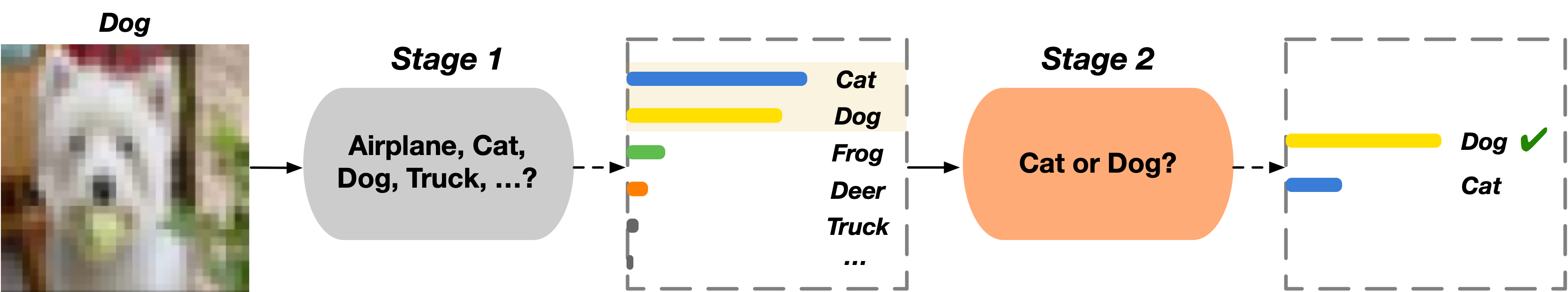
Figure 1: E-PixelHop is a two-stage sequential classification method.

The E-PixelHop method for object classification is proposed in this section. An overview of E-PixelHop is described in Sec. 3.1. Then, a multi-class classification baseline is described in Sec. 3.2. Finally, confusion class resolution is presented in Sec. 3.3.

3.1 System Overview

The overall framework of the E-PixelHop is illustrated in Fig. 1. It is a two-stage sequential classification method. The first stage serves as a baseline that performs classification among all object classes. Its output is a set of soft decision scores that indicate the probability of each class. The classes with the highest $M$ probabilities for each image as its confusing group. Typically, we set $M=2$. In the second stage, a one-versus-one competition is conducted to refine the prediction result. The two-stage sequential decision makes a coarse prediction and, then, focuses on confusing classes resolution for more accurate prediction.

We follow the traditional pattern recognition paradigm by dividing the problem into feature extraction and classification two separate modules. Multi-hop c/w Saab transforms are used to extract joint spatial-spectral features in an unsupervised manner. For classification, we adopt pixel-based classification in each hop that predicts objects of different scales at different spatial locations, where a pixel in a deeper hop denotes a patch of a larger size in the input image. In the training, ground truth labels at pixels follow image labels. Pixel-based classification based on the intra-hop information only tends to be noisy. To address this problem, a supervised label smoothing (SLS) method is proposed to reduce prediction uncertainty.

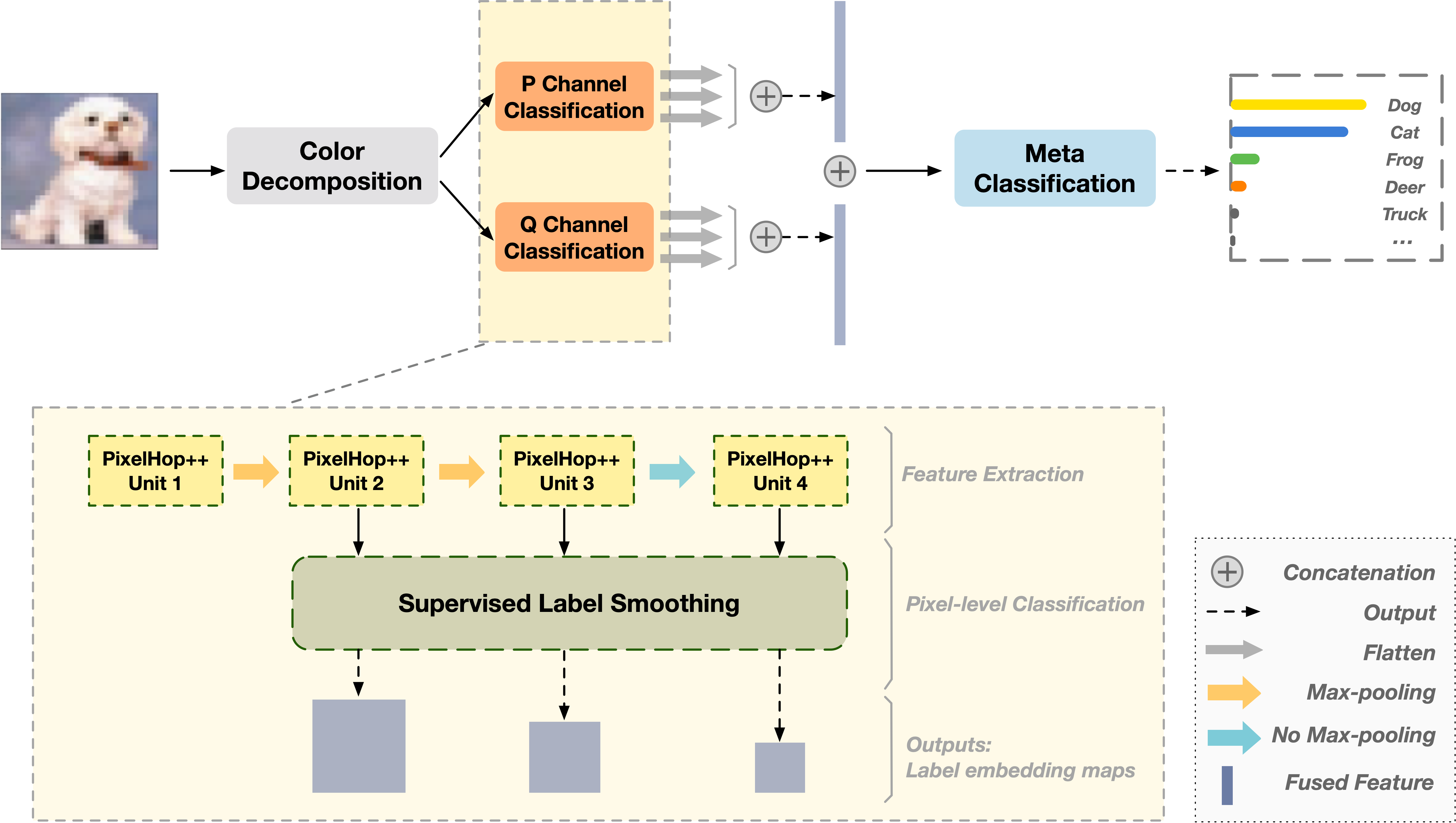
Figure 2: Illustration of the E-PixelHop classification baseline.

3.2 Stage 1: Multi-class Baseline Classifier

We use the CIFAR-10 dataset [42] as an example to explain the architecture of the multi-class classification baseline. It consists of four modules: 1) Color decomposition, 2) PixelHop++ feature extraction, 3) Pixel-level classification with label smoothing, 4) Meta classification. The system diagram for the baseline classification is shown in Fig. 2.

1) Color decomposition. For input color images of RGB three channels, the feature dimension is three times of the spatial dimension in a local neighborhood. To reduce the dimension, we apply the principle component analysis (PCA) to the 3D color channels of all pixels. That is, we collect RGB 3D color vectors from pixels in all input images and learn the PCA kernels from collected samples. They project the RGB color coordinates to decoupled color coordinates, which are named the PQR color coordinates, where P and Q channels correspond to the $1^{st}$ and $2^{nd}$ principle components. Experimental results show that P and Q channels contain approximately 98.5% of the energy of RGB three channels. Specifically, the P channel has 91.08% and the Q channel 7.38%. Since P and Q channels are uncorrelated with each other, we can proceed them separately in modules 2 and 3.

2) PixelHop++ feature extraction. As shown in Fig. 2, we use multiple PixelHop++ units [10] to extract features from P and Q channels, respectively. One PixelHop++ unit consists of two cascaded operations: 1) neighborhood construction with a defined window size in the spatial domain, and 2) the channel-wise (c/w) Saab transform. The input to the first PixelHop++ unit is a tensor of dimension $(S_{0}\times S_{0})\times K_{0}$, where $S_{0}\times S_{0}$ is the spatial dimension, $K_{0}$ is the spectral dimension, and subscript $0$ indicates that it is the hop-0 representation. For raw RGB images, $K_{0}=3$. Through color transformation, we have $K_{0}=1$ for each individual P or Q channel. The output of the $i$-th PixelHop++ unit is denoted by $(S_{i}\times S_{i})\times K_{i}$, which is the hop-$i$ representation. The hyper parameter $K_{i}$ is determined by the number of total c/w Saab coefficients kept in hop-$i$. As $i$ increases, the receptive field associated with a pixel in hop-$i$ becomes larger and more global information of the input image is captured. To enable faster expansion of the receptive field, we apply max-pooling with stride $2$ in shallower hops.

3) Pixel-level classification with label smoothing. The output from each PixelHop++ unit can be viewed as a feature tensor. The feature vector associated with a pixel location is fed into a pixel-level classifier to get a probability vector whose element indicates the probability of belonging to a certain object class. This probability vector can be viewed as a soft decision or a soft label. The soft label can be noisy, and we propose a supervised label smoothing mechanism to make the soft decision at neighboring spatial locations and hops more consistent. This is one of the main contributions of E-PixelHop. It will be elaborated in Sec. 4.

4) Meta classification. The soft decision maps from different hops of P and Q channels are concatenated and used to train a meta classifier, which gives the baseline prediction.

3.3 Stage 2: Confusion Set Resolution

Instead of constructing a hierarchical learning structure manually as done in [22], E-PixelHop identifies confusion sets using the predictions of the baseline classifier in Stage 1. The baseline classifier outputs a $C$-dimensional soft decision vector for each image. Generally, the $M$ classes with the highest probabilities can define a confusion set. For a $C$-class classification problem, we have at most $N_{cg}=\frac{C!}{M!(C-M)!}$ confusion sets. In practice, only a portion of $N_{cg}$ sets contribute to the performance gain significantly since the member of some confusion set is few. In the following, we focus on the case with $M=2$. The confusion matrix of the baseline classifier for CIFAR-10 is shown in Table 1. We see from the table that “Cat” and “Dog” are more likely to be confused with each other.

Without loss of generality, we use the “Cat and Dog” two confusing classes from CIFAR-10 as an example to explain our approach for confusion resolution. In the training, we collect all 5,000 Cat images and 5,000 Dog images from the training set. For test images that have the top-2 candidates of Cat or Dog, we include them in the Cat/Dog confusion set. If an image belongs to this set yet its ground truth class is neither Cat nor Dog, its misclassification cannot be corrected. As a result, the top-2 accuracy of the baseline classifier offers an upper bound for the final performance. For binary classification, the PixelHop++ features learned from the 10 classes in the baseline for P and Q channels are reused. Since the label is a 2-D vector whose element sum is equal to unity, we can simplify the label to a scalar in label smoothing. Thus, the lab map has a size of $S_{i}\times S_{i}\times 1$ at hop-$i$. We use the same ensemble scheme to fuse P and Q predicted labels. The meta classifier finally yields a binary decision for each test image in the confusion set to be a dog or a cat.

Table 1: The confusion matrix for the CIFAR-10 dataset, where the first row shows the predicted object labels and the first column shows the ground truth

	airplane	automobile	bird	cat	deer	dog	frog	horse	ship	truck
airplane	0.715	0.039	0.071	0.020	0.018	0.009	0.019	0.015	0.060	0.034
automobile	0.019	0.852	0.008	0.005	0.006	0.004	0.010	0.007	0.015	0.074
bird	0.059	0.006	0.639	0.069	0.077	0.047	0.065	0.024	0.007	0.007
cat	0.025	0.012	0.072	0.547	0.053	0.153	0.070	0.029	0.016	0.023
deer	0.016	0.007	0.049	0.029	0.694	0.045	0.060	0.089	0.007	0.004
dog	0.012	0.012	0.040	0.199	0.042	0.618	0.032	0.054	0.005	0.008
frog	0.007	0.005	0.044	0.056	0.030	0.027	0.815	0.002	0.011	0.003
horse	0.018	0.004	0.024	0.048	0.058	0.053	0.013	0.768	0.005	0.009
ship	0.047	0.025	0.014	0.008	0.004	0.005	0.008	0.005	0.858	0.026
truck	0.024	0.063	0.006	0.009	0.001	0.003	0.002	0.013	0.013	0.866

4 Supervised Label Smoothing

Soft label prediction at each pixel of a certain hop tends to be noisy. Label smoothing attempts to convert noisy decision to a clean one using adjacent label prediction from the same hop or from adjacent hops. The uncertainty of intra-hop prediction is first discussed in Sec. 4.1. The supervised label smoothing (SLS) scheme is then presented in Sec. 4.2.

4.1 Intra-Hop Prediction

For image classification, only the global coarse-scale information may not be sufficient. Mid-range to local fine-scale information can help characterize discriminant information of an region of interest. However, the object size varies a lot from images to images. Different receptive fields are needed for various object sizes and the context around objects. To exploit the characteristics of different scales, we do pixel-wise classification at each hop and ensemble predicted class probabilities from all hops. One naive approach is to use the extracted c/w Saab features of a single hop for classification, called intra-hop prediction. For example, c/w Saab features at hop-$i$ are of dimension $(S_{i}\times S_{i})\times K_{i}$, where $(S_{i}\times S_{i})$ and $K_{i}$ represent spatial and spectral dimensions, respectively. $N$ training images contribute $N\times S_{i}\times S_{i}$ training samples for intra-hop prediction. Each sample has a feature vector of dimension $K_{i}$. For the $n$-th training image, all $S_{i}\times S_{i}$ pixels share the same object label $y_{n}$. For the test image, the output of intra-hop prediction at hop-$i$ is a tensor of predicted class probabilities with the same spatial resolution of the input. The class probability vectors are soft decision labels of a pixel at hop-$i$, which corresponds to a spatial region of the input image with its size equal to the receptive field of the pixel.

Pixel-wise classification can be noisy since its training label is set to the image label. For a dog image, only part of the image contains discriminant dog characteristics while other part belongs to background and has nothing to do with dogs. On one hand, the shared background of dog and cat images will have two different labels in the training so that its prediction of dog or cat becomes less confident. On the other hand, the intra-hop classifier will be more confident in its predictions in regions that are associated with a particular class uniquely. For example, for a binary classification between a cat and a dog, contents in background such as grass and sofa are usually common so that the classifier is less confident in these regions as compared with the foreground regions that contain cat/dog faces.

4.2 Supervised Label Smoothing (SLS)

Since the decision at each pixel is made independently of others in pixel-level classification, there are local prediction fluctuations. We expect consistency in predictions in a spatial neighborhood as well as regions of a similar receptive field across hops that form a pyramid. To reduce the prediction fluctuation, we propose a supervised label smoothing scheme that iteratively uses predicted labels to enhance classification performance while keeping intra-hop and inter-hop consistency. It consists of three components: a) local graph construction; b) label initialization; and c) iterative cross-hop label update. A similar high-level idea was proposed in GraphHop [43], yet the details are different.

Local Graph Construction.

The tree-decomposed-structure of multi-Hop c/w Saab transforms corresponds to a directed graph. Each spatial location is a node. As shown in Fig. 3, we define three node types – child nodes, parent nodes, and sibling nodes. Hop-$i$ features are generated by an input of size $5\times 5$ through the c/w Saab transform from hop-$(i-1)$. The $5\times 5$ locations in hop-$(i-1)$ form $25$ child nodes for the orange node at hop-$i$. The orange node is then covered by a window of size $3\times 3$ to generate the green node in hop-$(i+1)$. Thus, it is one of the $9$ child nodes of the green node and the green node is the parent node of the orange one. As to sibling nodes, they are neighboring pixels at the same hop. Specifically, we consider eight nearest neighbors. The union of the eight neighbors and the center pixel form a $3\times 3$ window.

Label Initialization.

For the hop-$i$ feature tensor of dimension $S_{i}\times S_{i}\times K_{i}$, it consists of $S_{i}^{2}$ nodes. We treat each node at the same hop as a sample and train a classifier to generate a soft decision as its initial label. In the training, the image-level object class is propagated to all nodes at all hops. Only the c/w Saab features are used for label prediction initially, which is given by

$$\boldsymbol{Z}^{(0)}_{i,u,v}=h_{i}^{(0)}(\boldsymbol{f}_{i,u,v}),$$ (1)

where $\boldsymbol{Z}^{(0)}_{i,u,v}$ is the initial label prediction for node $(u,v)$ at hop-$i$, $\boldsymbol{f}_{i,u,v}$ is the corresponding c/w Saab feature vector and $h_{i}^{(0)}$ denotes the classifier. For the hops whose child nodes have label initialization, we concatenate the c/w Saab features and the label predicted in the previous hop to train the classifier. That is,

$$\boldsymbol{Z}^{(0)}_{i,u,v}=h_{i}^{(0)}(\boldsymbol{f}_{i,u,v}\oplus\boldsymbol{Z}^{(0)}_{i-1,{u},{v}}),$$ (2)

where the initial predicted label of $M\times N$ child nodes constructed by the local graph for node $(u,v)$ are averaged as

$$\boldsymbol{Z}^{(0)}_{i-1,{u},{v}}=\frac{1}{M\times N}\sum_{m=0}^{M-1}\sum_{n=0}^{N-1}\boldsymbol{Z}^{(0)}_{i-1,m,n}.$$ (3)

This is different from the intra-hop prediction because of the aggregation with child nodes and the inter-hop information is exchanged.

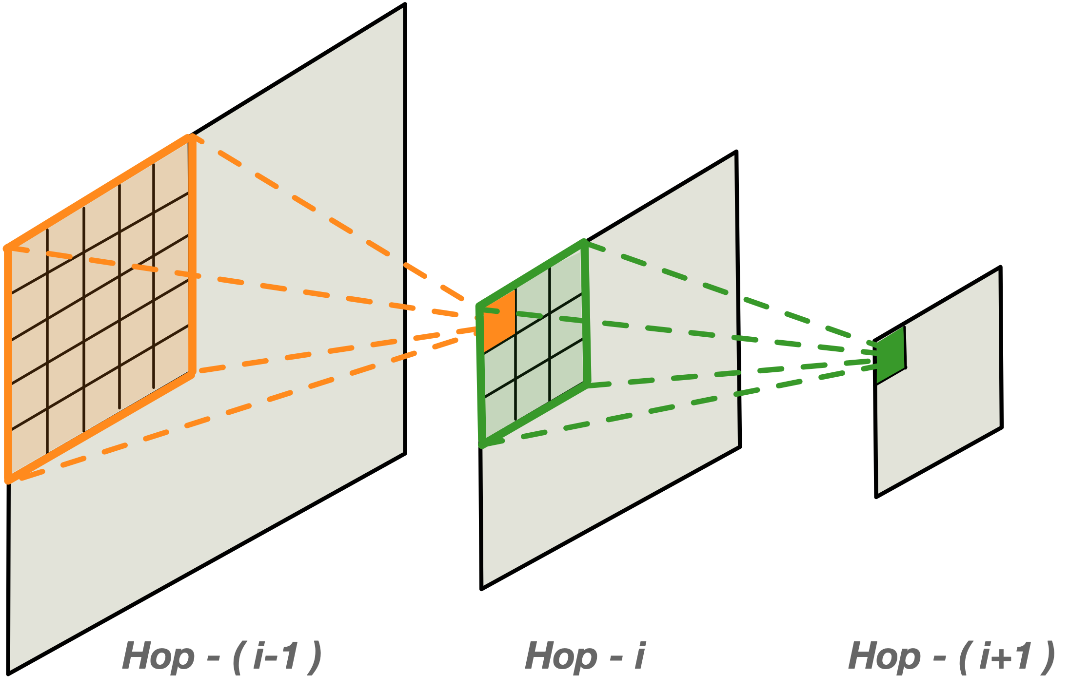
Figure 3: Illustration of local graph construction based on c/w Saab transforms.

Cross-hop Label Update.

Besides the intra-hop label update as described above, we conduct the inter-hop label update iteratively. The label is updated from the shallow hop to the deep hop as shown in Fig. 4 at each iteration. To update the label at the yellow location in hop-$i$, we gather the neighborhood that forms a pyramid. The labels are averaged among sibling and child nodes in blue and green regions, respectively. They are aggregated with labels of its parent node and itself. For a $C$-class classification scenario, the degree of freedom of the predicted soft label is $C-1$ so that the aggregated label dimension is equal to $4\times(C-1)$. For example, in the Cat/Dog confusion set with $C=2$, only the dimension corresponding to dog in the current label is extracted. This gives the aggregated feature of dimension 4-D. To control the model size, we do not use the c/w Saab feature for label update. A classifier is trained against the aggregated label dimension. The output soft decisions are the updated labels at iteration $k$ in form of

$$\boldsymbol{Z}^{(k)}_{i,u,v}=h_{i}^{(k-1)}(\boldsymbol{Z_{agg}}^{(k-1)}_{i,u,v}),$$ (4)

where $\boldsymbol{Z_{agg}}^{(k-1)}_{i,u,v}$ denotes the aggregated features of the cross-hop neighborhood.

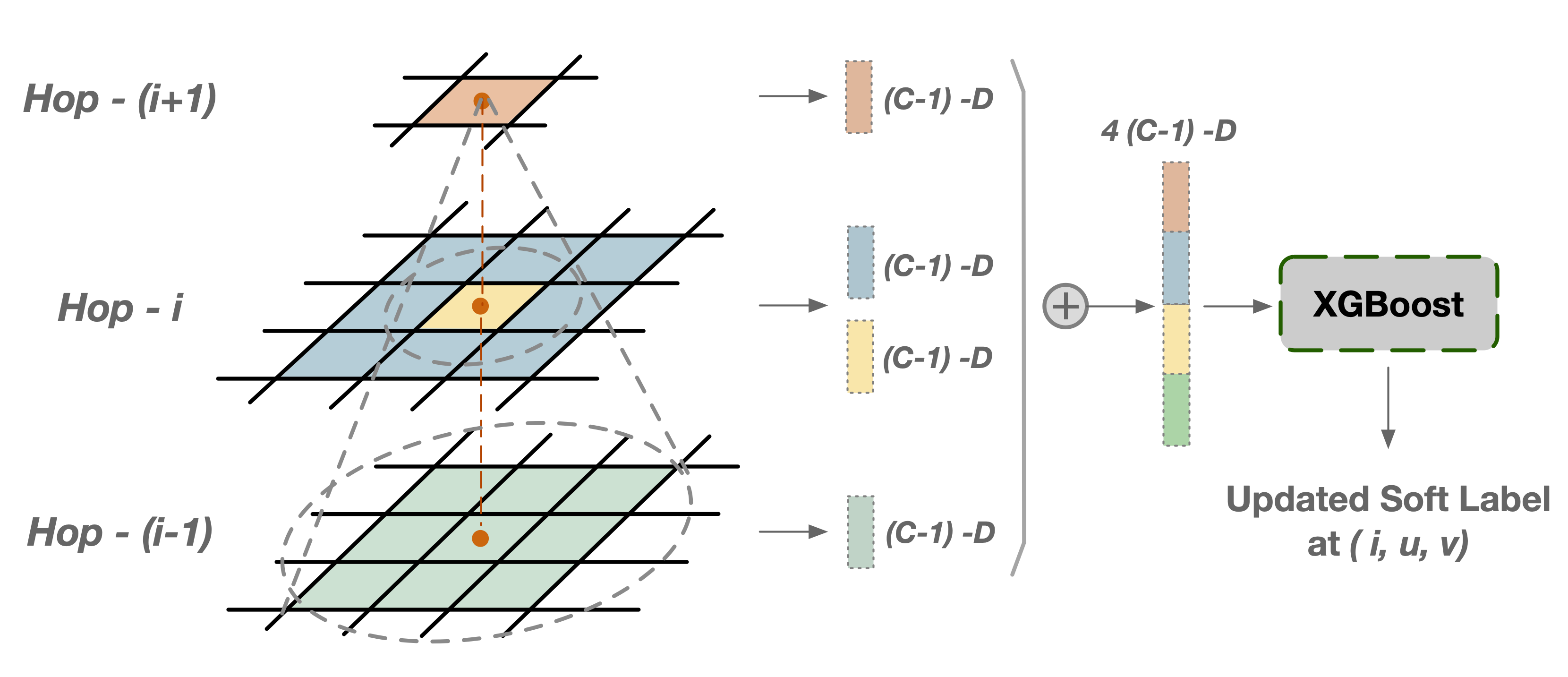
Figure 4: Illustration of inter-hop label updates.

5 Experiments

5.1 Experimental Setup

We evaluate the classification performance of E-PixelHop using the CIFAR-10 dataset that contains 10 classes of tiny color images of spatial resolution $32\times 32$. There are 50,000 training images and 10,000 test images. The hyper parameters of the PixelHop++ feature extraction architecture are listed in Table 2. The spectral dimensions are decided by energy thresholds in the c/w Saab transform.

For baseline classification in stage-1 and confusion class resolution in stage-2, we adopt different pixel-based prediction schemes. For stage-1, pixel-based prediction is conducted among three output feature maps, namely, hop-2 after max-pooling, hop-3 and hop-4. The SLS method without cross-hop label update is performed among these three hops. For stage-2, besides hop-3 and hop-4, we consider hop-2 without max-pooling for higher resolution to leverage more local information in distinguishing confusion classes. The full SLS method is conducted as the pixel-based prediction in stage-2. Yet, hop-1 features are not used since their receptive field is too small. We use the XGBoost (extreme gradient boosting) classifier for all classification tasks in E-PixelHop.

By following [4], we adopt data augmentation in both training and test for performance improvement. It includes original input images, random squared/rectangular croppings, contrast manipulation, horizontal flipping. Eight variants of each input are created. The Lanczos interpolation is applied to cropped images to resize them back to the $32\times 32$ resolution. In the test phase, classification soft decisions are averaged among the eight variants to get the final score for a test image.

Table 2: Hyper parameters of the PixelHop++ feature extraction architecture.

	Filter		Output Feature
	Window Size	Stride	Spatial	Spectral (P/Q)
Hop-1	$5\times 5$ (pad 2)	$1\times 1$	$32\times 32$	24 / 22
Max-pooling 1	$3\times 3$	$2\times 2$	$15\times 15$	24 / 22
Hop-2	$5\times 5$ (pad 2)	$1\times 1$	$15\times 15$	144 / 114
Max-pooling 2	$3\times 3$	$2\times 2$	$7\times 7$	144 / 114
Hop-3	$3\times 3$	$1\times 1$	$5\times 5$	203 / 174
Hop-4	$3\times 3$	$1\times 1$	$3\times 3$	211 / 185

5.2 Effects of Color Decomposition

E-PixelHop conducts classification in P and Q channels separately and then ensembles the classification results as shown in Fig. 2. We compare different ways to handle color channels for the baseline classifier in Table 3. Since the Q channel contains much less energy than the P channel, its classification performance is worse. The ensemble of P and Q channels outperforms the P channel alone by 3.46% and 2.83% in top-1 and top-2 accuracies, respectively. It shows that P and Q channels are complementary to each other.

Table 3: Comparison of test accuracy (%) in E-PixelHop baseline using different color channels

P channel	Q channel	Top-1	Top-2
✓		70.26	84.92
	✓	58.8	76.13
✓	✓	73.72	87.75

5.3 Confusion Sets Ranking

For a 10-class classification problem, we may have at most 45 confusion sets for one-versus-one competition. Two images form a confusion pair if they are the top-2 candidates in the baseline decision. The image number in each confusion set varies. For the second stage classification, we give a higher priority to confusion sets that have a large number of pairs and plot the test accuracy as a function of the total resolved confusing sets in Fig. 5. The test accuracy increases as more confusion sets are resolved and saturates after 27 sets are taken care of.

Figure 5: The plot of CIFAR-10 test accuracy (%) as a function of the cumulative number of resolved confusion sets.

5.4 Effects of Supervised Label Smoothing (SLS)

To demonstrate the power of SLS, we study the binary classification problem and show the results in Table 4 for four frequent confusion sets: Cat vs Dog, Airplane vs Ship, Automobiles vs Truck, and Deer vs Horse. The training set includes 5,000 images while the test set contains 1,000 images from each of the two classes. For pixel-based classification, we examine test accuracies of intra-hop prediction and the addition of supervised label smoothing (SLS), where results of P and Q channels are ensembled. We see from the table that the addition of SLS outperforms that without SLS by 2%$\sim$3% in all four confusing sets.

Table 4: Comparison of image-level test accuracy (%) for four confusion sets with and without SLS.

Confusing Group	intra-hop only	intra-hop and SLS
Cat vs Dog	76.45	79.1
Airplane vs Ship	92.1	93.75
Automobile vs Truck	89.8	92.95
Deer vs Horse	87.8	90.95

Figure 6: Illustration of intermediate label maps for different methods, where each subfigure shows label heatmaps in hop-2, hop-3 and hop-4 (from left to right).

To understand the behavior of SLS furthermore, we show intermediate label maps in heat maps from hop-2 to hop-4 for three Dog images in Fig. 6 with three schemes: a) intra-hop prediction, b) one iteration of SLS label initialization only and c) SLS with another iteration of cross-hop label update. The heatmaps indicate the confidence score at each pixel location for the Dog class. For the hop-2 heatmaps, regions composed by the dog face have higher Dog confidence than other regions. By comparing Figs. 6(a) and (b), we see an increase in the highest confidence level in hop-3 using one round of SLS label initialization. Clearly, SLS makes label maps more distinguishable. Furthermore, heatmaps are more consistent across hops in Fig. 6(b). After one more SLS iteration of cross-hop update, the confidence scores become more homogeneous in a neighborhood as shown in Fig. 6(c), where more locations agree with each other and with the ground truth label.

Figure 7: Pixel-level test accuracy in hop-2, hop-3 and hop-4 and the image-level ensemble as a function of iteration numbers for P-channel images only.

Since SLS is an iterative process, we show the pixel-level accuracy and the final image-level accuracy as a function of the iteration number for the four confusion sets discussed earlier in Fig. 7. The first point is the initial label in SLS. We see that the pixel-level accuracy at each hop increases rapidly in first several iterations. This is especially obvious in shallow hops. Then, these curves converge at a certain level. In the experiments, we set the maximum number of iterations to num_iter = 3 for the one-versus-one confusion set resolution to avoid over-smoothing. In the 10-class baseline, we set num_iter = 1 (i.e. only the initialization of SLS) by taking both inter-hop guidance and model complexity into account.

Although the pixel-level accuracy saturates at the same level for all three hops, the ensemble performance (in red dashed line) is better than that of each individual hop as shown in Fig. 7. As the iteration number increases, the ensemble result also increases and saturates in 3 to 5 iterations although the increment is smaller than that of the pixel-level accuracy.

Table 5: Ablation study of E-PixelHop’s components for CIFAR-10

Augmentation	Color Channels		Baseline		2-nd pipeline		Test Accuracy
	P channel	Q channel	intra-hop	SLS_init	intra-Hop	SLS
	✓	✓		✓			68.69
✓	✓			✓			70.26
✓	✓	✓		✓			73.72
✓	✓	✓	✓				72.29
✓	✓	✓		✓	✓		72.79
✓	✓	✓		✓		✓	76.18
✓	✓	✓	✓			✓	75.54

5.5 Ablation Study and Performance Benchmarking

The ablation study of adopting various components in E-PixelHop is summarized in Table 5, where the image-level test accuracy for CIFAR-10 is given in the last column. The study includes: data augmentation, color channel decomposition, the methods of pixel-level classification in the baseline and in confusion set resolution, respectively. The first four rows show the baseline performance without confusion set resolution while the last three rows have both. For pixel-level classification, the intra-hop column does not have label smoothing while the SLS_init column has SLS initialization only. Moreover, the pixel-level classification in the baseline does not use augmented images to train classifiers by considering the time and model complexity. Data augmentation is only used for the meta classification in the baseline and one-versus-one competition in confusion set resolution. The E-PixelHop baseline achieves test accuracy of 73.72% using both P/Q channels with SLS initialization for pixel-level classification and data augmentation when training the meta classifier. By further adding the $2^{nd}$ pipeline with three SLS iterations in pixel-level classification, E-PixelHop achieves a test accuracy of 76.18% as shown in the sixth row, where all 45 confusing sets are processed.

We compare the performance of six methods in Table 6. They are modeified LeNet-5 [1], PixelHop [9], PixelHop⁺ [9] and PixelHop++ [10], the E-PixelHop baseline, and the complete E-PixelHop. To handle color images, we modify the LeNet-5 network architectures slightly, whose hyper parameters are given in Table 7. Both the E-PixelHop baseline and the complete E-PixelHop outperform other benchmarking methods. An improvement of 9.37% over PixelHop++ and an improvement of 3.52% over PixelHop⁺ are observed, respectively.

Table 6: Comparison of testing accuracy (%) of LeNet-5, PixelHop, PixelHop+ and PixelHop++ for CIFAR-10.

	Test Accuracy (%)
Lenet-5	68.72
PixelHop [9]	71.37
PixelHop+ [9]	72.66
PixelHop++ [10]	66.81
E-PixelHop Baseline (Ours)	73.72
E-PixelHop (Ours)	76.18

Table 7: Hyper parameters of the modified LeNet-5 network as compared with those of the original LeNet-5.

	Original LeNet-5	Modified LeNet-5
Conv-1 Kernel Size	5x5x1	5x5x3
Conv-1 Kernel No.	6	32
Conv-2 Kernel Size	5x5x6	5x5x32
Conv-2 Kernel No.	16	64
FC-1	120	200
FC-2	84	100
Output Layer	10	10

6 Conclusion and Future Work

An enhanced SSL-based object classification method called E-PixelHop was proposed in this work. It has two classification stages: multi-class classification in the first stage and the confusion set resolution in the second stage. Supervised label smoothing (SLS) was proposed to enhance the performance and ensure consistency of intra-hop and inter-hop pixel-level predictions. Effectiveness of SLS shows the importance of prediction agreement at different scales. Furthermore, it is important to handle confusing classes carefully so that the overall classification performance can be boosted.

For the second-stage classification, all training images in the confusion set are used to train the one-versus-one model in the current E-PixelHop. In the future, it is worthwhile to investigate boosting with hard cases mining and learn from errors. Furthermore, not every pixel in an image is discriminant and salient. We should find a way to focus on discriminant regions by introducing an attention mechanism. It is also desired to generalize our work to the recognition of a larger number of classes (e.g., CIFAR-100) and higher image resolution (e.g., the ImageNet).

References

- [1] Y. LeCun, L. Bottou, Y. Bengio, and P. Haffner, “Gradient-based learning applied to document recognition,” Proceedings of the IEEE, vol. 86, no. 11, pp. 2278–2324, 1998.
- [2] K. He, X. Zhang, S. Ren, and J. Sun, “Deep residual learning for image recognition,” in Proceedings of the IEEE conference on computer vision and pattern recognition, pp. 770–778, 2016.
- [3] G. Huang, Z. Liu, L. Van Der Maaten, and K. Q. Weinberger, “Densely connected convolutional networks,” in Proceedings of the IEEE conference on computer vision and pattern recognition, pp. 4700–4708, 2017.
- [4] K. Simonyan and A. Zisserman, “Very deep convolutional networks for large-scale image recognition,” arXiv preprint arXiv:1409.1556, 2014.
- [5] C. Szegedy, W. Liu, Y. Jia, P. Sermanet, S. Reed, D. Anguelov, D. Erhan, V. Vanhoucke, and A. Rabinovich, “Going deeper with convolutions,” in Proceedings of the IEEE conference on computer vision and pattern recognition, pp. 1–9, 2015.
- [6] F. N. Iandola, S. Han, M. W. Moskewicz, K. Ashraf, W. J. Dally, and K. Keutzer, “Squeezenet: Alexnet-level accuracy with 50x fewer parameters and< 0.5 mb model size,” arXiv preprint arXiv:1602.07360, 2016.
- [7] A. G. Howard, M. Zhu, B. Chen, D. Kalenichenko, W. Wang, T. Weyand, M. Andreetto, and H. Adam, “Mobilenets: Efficient convolutional neural networks for mobile vision applications,” arXiv preprint arXiv:1704.04861, 2017.
- [8] M. Tan and Q. Le, “Efficientnet: Rethinking model scaling for convolutional neural networks,” in International Conference on Machine Learning, pp. 6105–6114, PMLR, 2019.
- [9] Y. Chen and C.-C. J. Kuo, “Pixelhop: A successive subspace learning (ssl) method for object recognition,” Journal of Visual Communication and Image Representation, vol. 70, p. 102749, 2020.
- [10] Y. Chen, M. Rouhsedaghat, S. You, R. Rao, and C.-C. J. Kuo, “Pixelhop++: A small successive-subspace-learning-based (ssl-based) model for image classification,” in 2020 IEEE International Conference on Image Processing (ICIP), pp. 3294–3298, IEEE, 2020.
- [11] J. Mutch and D. G. Lowe, “Multiclass object recognition with sparse, localized features,” in 2006 IEEE Computer Society Conference on Computer Vision and Pattern Recognition (CVPR’06), vol. 1, pp. 11–18, IEEE, 2006.
- [12] P. Schnitzspan, M. Fritz, and B. Schiele, “Hierarchical support vector random fields: Joint training to combine local and global features,” in European conference on computer vision, pp. 527–540, Springer, 2008.
- [13] L. Liu, C. Shen, and A. van den Hengel, “The treasure beneath convolutional layers: Cross-convolutional-layer pooling for image classification,” in Proceedings of the IEEE Conference on Computer Vision and Pattern Recognition, pp. 4749–4757, 2015.
- [14] S. Jetley, N. A. Lord, N. Lee, and P. H. Torr, “Learn to pay attention,” arXiv preprint arXiv:1804.02391, 2018.
- [15] W. Liu, I. W. Tsang, and K.-R. Müller, “An easy-to-hard learning paradigm for multiple classes and multiple labels,” The Journal of Machine Learning Research, vol. 18, 2017.
- [16] Y. Seo and K.-s. Shin, “Hierarchical convolutional neural networks for fashion image classification,” Expert systems with applications, vol. 116, pp. 328–339, 2019.
- [17] A. Zweig and D. Weinshall, “Exploiting object hierarchy: Combining models from different category levels,” in 2007 IEEE 11th International Conference on Computer Vision, pp. 1–8, IEEE, 2007.
- [18] A. Bilal, A. Jourabloo, M. Ye, X. Liu, and L. Ren, “Do convolutional neural networks learn class hierarchy?,” IEEE transactions on visualization and computer graphics, vol. 24, no. 1, pp. 152–162, 2017.
- [19] Z. Yan, H. Zhang, R. Piramuthu, V. Jagadeesh, D. DeCoste, W. Di, and Y. Yu, “Hd-cnn: hierarchical deep convolutional neural networks for large scale visual recognition,” in Proceedings of the IEEE international conference on computer vision, pp. 2740–2748, 2015.
- [20] C. Chen, S. Li, X. Fu, Y. Ren, Y. Chen, and C.-C. J. Kuo, “Exploring confusing scene classes for the places dataset: Insights and solutions,” in 2017 Asia-Pacific Signal and Information Processing Association Annual Summit and Conference (APSIPA ASC), pp. 550–558, IEEE, 2017.
- [21] S. Li, C. Chen, Y. Ren, and C.-C. J. Kuo, “Improving object classification performance via confusing categories study,” in 2018 IEEE Winter Conference on Applications of Computer Vision (WACV), pp. 1774–1783, IEEE, 2018.
- [22] X. Zhu and M. Bain, “B-cnn: branch convolutional neural network for hierarchical classification,” arXiv preprint arXiv:1709.09890, 2017.
- [23] C.-C. J. Kuo, “Understanding convolutional neural networks with a mathematical model,” Journal of Visual Communication and Image Representation, vol. 41, pp. 406–413, 2016.
- [24] C.-C. J. Kuo, “The cnn as a guided multilayer recos transform [lecture notes],” IEEE signal processing magazine, vol. 34, no. 3, pp. 81–89, 2017.
- [25] C.-C. J. Kuo and Y. Chen, “On data-driven saak transform,” Journal of Visual Communication and Image Representation, vol. 50, pp. 237–246, 2018.
- [26] C.-C. J. Kuo, M. Zhang, S. Li, J. Duan, and Y. Chen, “Interpretable convolutional neural networks via feedforward design,” Journal of Visual Communication and Image Representation, 2019.
- [27] Y. Chen, Z. Xu, S. Cai, Y. Lang, and C.-C. J. Kuo, “A saak transform approach to efficient, scalable and robust handwritten digits recognition,” in 2018 Picture Coding Symposium (PCS), pp. 174–178, IEEE, 2018.
- [28] Y. Chen, Y. Yang, W. Wang, and C.-C. J. Kuo, “Ensembles of feedforward-designed convolutional neural networks,” in 2019 IEEE International Conference on Image Processing (ICIP), pp. 3796–3800, IEEE, 2019.
- [29] M. Zhang, Y. Wang, P. Kadam, S. Liu, and C.-C. J. Kuo, “Pointhop++: A lightweight learning model on point sets for 3d classification,” in 2020 IEEE International Conference on Image Processing (ICIP), pp. 3319–3323, IEEE, 2020.
- [30] M. Zhang, H. You, P. Kadam, S. Liu, and C.-C. J. Kuo, “Pointhop: An explainable machine learning method for point cloud classification,” IEEE Transactions on Multimedia, 2020.
- [31] M. Zhang, P. Kadam, S. Liu, and C.-C. J. Kuo, “Unsupervised feedforward feature (uff) learning for point cloud classification and segmentation,” in 2020 IEEE International Conference on Visual Communications and Image Processing (VCIP), pp. 144–147, IEEE, 2020.
- [32] P. Kadam, M. Zhang, S. Liu, and C.-C. J. Kuo, “Unsupervised point cloud registration via salient points analysis (spa),” in 2020 IEEE International Conference on Visual Communications and Image Processing (VCIP), pp. 5–8, IEEE, 2020.
- [33] A. Manimaran, T. Ramanathan, S. You, and C.-C. J. Kuo, “Visualization, discriminability and applications of interpretable saak features,” Journal of Visual Communication and Image Representation, vol. 66, p. 102699, 2020.
- [34] T.-W. Tseng, K.-J. Yang, C.-C. J. Kuo, and S.-H. Tsai, “An interpretable compression and classification system: Theory and applications,” IEEE Access, vol. 8, pp. 143962–143974, 2020.
- [35] M. Rouhsedaghat, Y. Wang, X. Ge, S. Hu, S. You, and C.-C. J. Kuo, “Facehop: A light-weight low-resolution face gender classification method,” arXiv preprint arXiv:2007.09510, 2020.
- [36] X. Lei, G. Zhao, and C.-C. J. Kuo, “Nites: A non-parametric interpretable texture synthesis method,” in 2020 Asia-Pacific Signal and Information Processing Association Annual Summit and Conference (APSIPA ASC), pp. 1698–1706, IEEE, 2020.
- [37] M. Rouhsedaghat, M. Monajatipoor, Z. Azizi, and C.-C. J. Kuo, “Successive subspace learning: An overview,” arXiv preprint arXiv:2103.00121, 2021.
- [38] H.-S. Chen, M. Rouhsedaghat, H. Ghani, S. Hu, S. You, and C.-C. J. Kuo, “Defakehop: A light-weight high-performance deepfake detector,” in 2021 IEEE International Conference on Multimedia and Expo (ICME), pp. 1–6, IEEE, 2021.
- [39] K. Zhang, B. Wang, W. Wang, F. Sohrab, M. Gabbouj, and C.-C. J. Kuo, “Anomalyhop: An ssl-based image anomaly localization method,” arXiv preprint arXiv:2105.03797, 2021.
- [40] P. Kadam, M. Zhang, S. Liu, and C.-C. J. Kuo, “R-pointhop: A green, accurate and unsupervised point cloud registration method,” arXiv preprint arXiv:2103.08129, 2021.
- [41] X. Liu, F. Xing, C. Yang, C.-C. J. Kuo, S. Babu, G. E. Fakhri, T. Jenkins, and J. Woo, “Voxelhop: Successive subspace learning for als disease classification using structural mri,” arXiv preprint arXiv:2101.05131, 2021.
- [42] A. Krizhevsky and G. Hinton, “Learning multiple layers of features from tiny images,” tech. rep., University of Toronto, Toronto, Ontario, 2009.
- [43] T. Xie, B. Wang, and C.-C. J. Kuo, “Graphhop: An enhanced label propagation method for node classification,” arXiv preprint arXiv:2101.02326, 2021.