Disentangle Your Dense Object Detector

Abstract.

Deep learning-based dense object detectors have achieved great success in the past few years and have been applied to numerous multimedia applications such as video understanding. However, the current training pipeline for dense detectors is compromised to lots of conjunctions that may not hold. In this paper, we investigate three such important conjunctions: 1) only samples assigned as positive in classification head are used to train the regression head; 2) classification and regression share the same input feature and computational fields defined by the parallel head architecture; and 3) samples distributed in different feature pyramid layers are treated equally when computing the loss. We first carry out a series of pilot experiments to show disentangling such conjunctions can lead to persistent performance improvement. Then, based on these findings, we propose Disentangled Dense Object Detector (DDOD), in which simple and effective disentanglement mechanisms are designed and integrated into the current state-of-the-art dense object detectors. Extensive experiments on MS COCO benchmark show that our approach can lead to 2.0 mAP, 2.4 mAP and 2.2 mAP absolute improvements on RetinaNet, FCOS, and ATSS baselines with negligible extra overhead. Notably, our best model reaches 55.0 mAP on the COCO test-dev set and 93.5 AP on the hard subset of WIDER FACE, achieving new state-of-the-art performance on these two competitive benchmarks. Code is available at https://github.com/zehuichen123/DDOD.

1. Introduction

With the recent advance of deep learning, visual object detection has achieved massive progress in both performance and speed (Bochkovskiy et al., 2020; Wang et al., 2020a; Lin et al., 2017b). It has become the foundation for widespread multimedia applications, such as animation editing and interactive video games. Compared with the pioneering two-stage object detectors (Ren et al., 2015; Cai and Vasconcelos, 2018), single-stage dense detectors have received increasing attentions because of their simple and elegant pipeline. It directly outputs the detected bounding boxes, which ensures a fast inference speed, making it more suitable to be deployed on edge-computing devices.

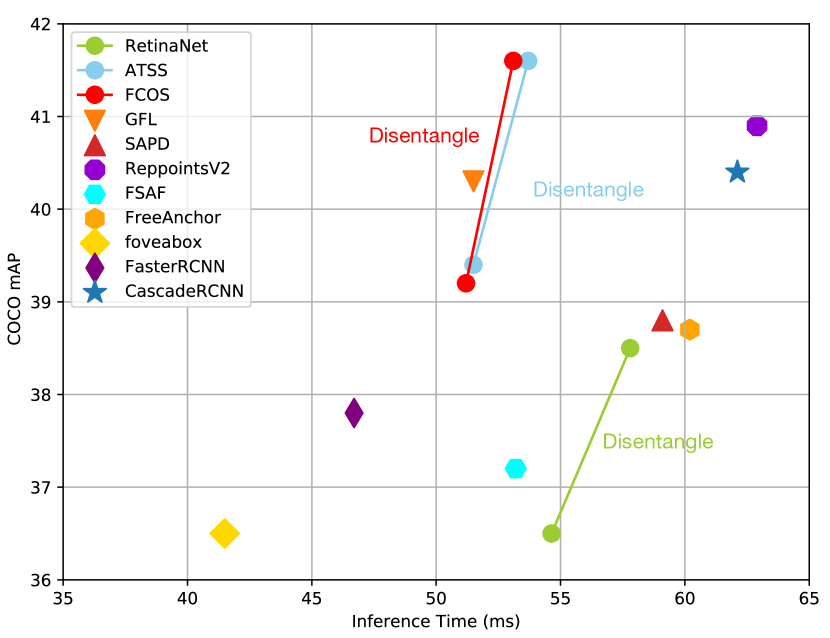
Figure 1. Our DDOD can improve the performance of different state-of-the-art dense object detectors with negligible extra inference time.

A typical dense object detector is composed of three parts: 1) a backbone network, usually pretrained on ImageNet (Deng et al., 2009), that extracts useful features from the input image and outputs multi-scale feature maps to detect objects at various scales; 2) a feature pyramid network (FPN) (Lin et al., 2017a) that further improves the multi-scale feature maps through feature fusion, in which shadow features are promoted by high-level semantic features from deeper layers; 3) a detection head that usually contains two branches to output the corresponding classification and bounding box regression results at each anchor point in the input feature map.

Since the first dense detector DenseBox (Huang et al., 2015) is proposed, hundreds of work has enhanced the performance, both in accuracy and speed. For example, Focal loss (Lin et al., 2017b) is one of the most prominent methods. It lowers down the gradient magnitude of well-classified samples, hence forcing the model to concentrate on hard samples. Recently, several anchor-free detectors have been proposed to remove the labor-intense anchor designing procedure. Other techniques (Wang et al., 2020b; Sun et al., 2020) focus on label assignment where the classic IoU threshold is replaced with more meticulous strategies. In a recent approach (Jiang et al., 2018), a localization quality estimation branch is added to the detection head to help with keeping high-quality boxes during non-maximum-suppression (NMS).

Although many algorithms have been proposed to improve the performance of dense detectors, the room for further improvement is still large. Specifically, we notice that there are several conjunctions in the training process of dense detectors that can lead to performance deterioration. These conjunctions are usually the compromises of engineering implementations, which seem reasonable but have not been studied thoroughly before.

Firstly, the regression loss is only applied to the positive samples of classification branch. This design sounds correct because we only care about the localization of foreground objects. However, will other samples benefit the training of the regression head?

Secondly, regardless of what the final bounding box looks like, the receptive fields, defined by several consecutive convolution operations, for classification and regression tasks are exactly the same. However, as pointed out in (Song et al., 2020), these two tasks have different preferences: classification desires regions with rich semantic information while regression prefers to attend edge parts. Therefore, the same receptive fields cannot guarantee the optimal performance.

Finally, there is an imbalance problem lying in the pyramid layers because of the same supervision on all training samples. Concretely, the number of training samples on $P_{3}$ level is 256 ($2^{8}$) times to that on $P_{7}$. Thus, concatenating them together to compute the training loss will result in extremely imbalanced supervision among samples on different layers, as the shallow layers receives much more supervision than deeper layers like $P_{7}$.

To summarize, the aforementioned conjunctions can be divided into three types: 1) the label assignment conjunction that the regression branch is only trained using the positive samples in classification branch; 2) the spatial feature conjunction between classification and regression where the same receptive field makes the model attend the same area of the feature map; 3) the pyramid supervision conjunction between different layers of FPN, in which the results on different layers are flattened and concatenated for loss computation, leading to the same supervision of all the layers.

In this paper, we first carry out a series of meticulously designed pilot experiments to show that disentangling such conjunctions can significantly improve the overall detection performance. Then, we propose a new training pipeline for dense object detectors called DDOD (Disentangled Dense Object Detector) with excellent performance, as illustrated in Figure 1. Specifically, for the assignment conjunction, we design separated label assigners for classification and regression, enabling us to pick out the most suitable training sets for those two branches, respectively. As for the spatial feature conjunction, an adaptive feature disentanglement module based on deformable convolution is proposed to automatically attend different features that benefit classification and regression. Finally, for the pyramid supervision conjunction, we design a novel re-weighting mechanism to adaptively adjust the magnitude of supervision on different FPN layers based on the positive samples on each layer.

The main contributions of this work are three-fold:

• We carry out detailed experiments to investigate three types of training conjunctions in dense object detectors, which are usually ignored by previous work but can cause performance deterioration.

• We propose to decouple these conjunctions in a unified detection framework called DDOD, which consists of label assignment disentanglement, spatial feature alignment disentanglement and pyramid supervision disentanglement.

• Through extensive experiments, we validate the effectiveness of the proposed DDOD on two competitive dense object detectors and achieve state-of-the-art performance on both COCO and WIDER FACE datasets.

2. Related Work

2.1. Label Assignment in Object Detection

Selecting which anchors are to be designated as positive or negative labels has been viewed as a crucial task, affecting the detector performance greatly. A vanilla practice is to assign anchors whose IoUs with the ground truth are greater than a certain threshold (Lin et al., 2017b; Ren et al., 2015). With the advance of anchor-free models, a new strategy for defining labels was proposed by FCOS (Tian et al., 2019), which directly views points inside GT boxes as positives. FreeAnchor (Zhang et al., 2021) constructs a bag of anchor candidates for each GT and solves the label assignment as a problem of detection-customized likelihood optimization. ATSS (Zhang et al., 2020b) suggests an adaptive anchor assignment which is calculated by the statistics from the mean and standard deviation of IoU values on a set of anchors for each GT. In order to adaptively separate anchors according to the models’s learning status, PAA (Kim and Lee, 2020) investigates a probabilistic manner to assign labels. However, these methods do not discuss the label conjunction between classification and regression branches.

2.2. Feature Alignment in Object Detection

Better feature alignment always indicates better performance. CascadeRPN  (Vu et al., 2019), GuidedAnchor  (Wang et al., 2019) and AlignDet  (Chen et al., 2019a) adopt a cascade-manner to improve the feature representation via re-aligning features. By re-extracting features at the afore-regressed bounding boxes, one can predict more precise classification scores and regression boxes. Besides, There are a variety of approaches that discuss the feature representation conjunction in classification and regression tasks on two-stage detectors. DoubleHead (Wu et al., 2020a) is the first one to find this phenomenon and proposes separate heads with different structures for classification and regression heads. TSD (Song et al., 2020) improves the ”shared head for classification and localization” (sibling head), firstly demonstrated in Fast RCNN by adopting different RoIAlign offsets for classification and regression. Although this conjunction has been validated and well-addressed in two-stage methods, whether this problem exist in dense detectors remains an open problem.

2.3. Imbalanced Learning in Object Detection

Imbalanced learning exists in various aspects for many object detection frameworks (Pang et al., 2019; Oksuz et al., 2020). Alleviating such unbalance issues are crucial to attain satisfying detection results. RetinaNet (Lin et al., 2017b) proposes Focal loss to conquer extreme imbalance problem between the number of samples in positive and negative, which enables us to train dense object detectors without sampling strategy. Pang et al. (Pang et al., 2019) noticed that the detection performance is often limited by the imbalance during the training process, which generally consists in three aspects, namely the sample level, feature level and objective level. To address the above issues, Libra-RCNN is proposed to mitigate such gaps with IoU-balanced sampling, balanced feature pyramid, and balanced L₁ loss. Besides, the category imbalance is also a vital topic in object detection (Tan et al., 2020b, a; Wu et al., 2020b). EQL (Tan et al., 2020b) finds the accumulation of backward gradients from negative samples is larger than those from positive samples in rare categories, which results in the insufficient training on infrequent classes. Therefore, an equalization loss was proposed to moderate such a phenomenon.

In comparison, our work aims to disentangle these three important conjunctions in state-of-the-art dense object detectors to achieve better accuracy with minimum cost.

3. Pilot Experiments

In this section, we present our motivation by carrying out pilot experiments to show the harm of three conjunctions in dense object detectors and the possibility to advance the detection performance by disentanglement.

3.1. Label Assignment Conjunction

The assignment conjunction refers to the case that the regression loss is only applied to the ”foreground” samples in classification task. Actually, this conjunction is here for historical reasons. The concept of bounding box regression was first introduced in (Girshick et al., 2014), in which a smooth L₁ loss is used to train the regression branch. Applying the regression loss only to positive samples, whose IoU with the GT box is larger than a threshold, ensures the network to get enough information from the feature map for estimating the actual location of the object. However, this threshold does not need to coordinate with the classification threshold, and there is no such ”positive” concept when inferring as every anchor box or center point will be applied with its predicted regressor. Thus, setting a separate threshold for bounding box regression is reasonable. To validate our assumption, we train different RetinaNet models with various classification and regression IoU thresholds ranging from 0.4 to 0.6 and report the results in Table 1. It can be seen that the optimal performance, with a mAP of 36.5, is achieved with an IoU of 0.5 on classification head and 0.4 on regression head. Therefore, in our DDOD, we decompose the assignment conjunction by adopting respective label assigners on classification and regression branches for better detection accuracy.

Table 1. AP performance with different IoU thresholds for classification and regression branches on label assignment.

	0.4	0.5	0.6
0.4	35.0	35.3	33.2
0.5	36.5	36.1	35.3
0.6	34.6	35.2	35.1

3.2. Spatial Feature Conjunction

In a typical dense object detector, two parallel branches with the same structure are used for classification and regression, which implies that their corresponding receptive areas in the feature maps are the same. However, as pointed in TSD (Song et al., 2020), in two stage detectors these two tasks should concentrate on different parts of the objects: regions that is rich of semantic information is helpful for classification while the contour areas are essential for localization. We argue that this principle also holds for dense detectors. In Figure 2, we visualize the sensitive regions using GradCAM (Zhou et al., 2018) for classification and regression and find that they are indeed different, which validates the necessity to disentangle their receptive regions. In Section 4.2, we will describe a simple design to achieve this goal by adding an adaptive feature disentanglement module in both branches.

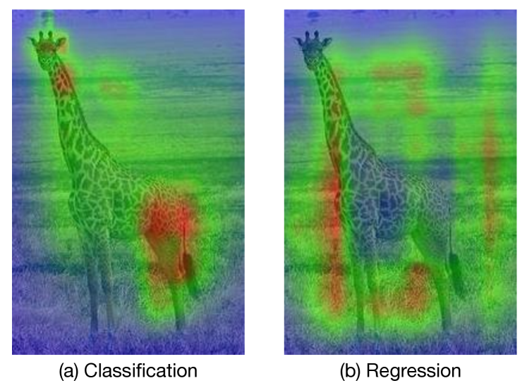
Figure 2. Visualization of backward gradient on the output of FPN. The heatmap is obtained by utilizing GradCAM (Zhou et al., 2018).

3.3. Supervision Conjunction in FPN

In the commonly adopted implementation of feature pyramid-based dense detectors, the predictions of different layers are ”flatten and concatenated” for loss computation, making the supervision on different layers to be conjectural. However, as pointed out in (Yang et al., 2021), the sample distribution is significantly imbalanced between different layers, because the feature size grows up in quadratic as the feature resolution increases. As a result, the training samples will be dominated by samples in lower levels, making the high-level samples lack of supervision, which will harm the performance on large objects. A simple idea to overcome this is to assign a larger weight to high-level samples to compensate for the supervision. In Table 2, we exploit different re-weighting strategies, where only the weights for lowest and highest layers are set and the rest ones are linearly interpolated. The best strategy is to linearly increase the weight from 1.0 to 2.0 and the worst one is to linearly decrease the weight from 3.0 to 1.0. This result validates our assumption and inspires us to propose an effective re-weighting approach called FPN hierarchical loss to disentangle the supervision conjunction.

Table 2. AP performance with linear increasing (decreasing) supervision weights from $P_{3}$ to $P_{7}$ levels on ATSS baseline.

re-weighting factor	AP	AP50	AP75	APS	APM	APL
1$\sim$1	39.4	56.6	42.6	23.9	42.5	49.6
1$\sim$2	39.8	57.8	42.9	22.9	43.5	51.8
1$\sim$3	39.4	56.7	42.9	21.6	43.1	52.0
2$\sim$1	38.7	56.6	42.1	23.2	42.7	48.3
3$\sim$1	37.6	55.3	40.8	22.2	41.6	47.0

4. Methodologies

In this section, we describe the proposed DDOD in detail. An overview of our approach is presented in Figure 3.

4.1. Label Assignment Disentanglement

One of the most widely accepted practice in label assignment is to only regress samples that are assigned as positives in the classification branch. However, as exploited in Section 3.1, such a conjunction between the two branches is suboptimal. Motivated by this observation, we design different label assignment strategies for classification and regression, respectively. In the early work, IoU between the candidate anchor and the ground truth is the only criterion for foreground-background assignment. Recently, some good attempts show that replacing IoU with the loss value is a more suitable approach for label assignment. Thus, we adopt a clean and effective cost formulation proposed in (Wang et al., 2020b) to mine more appropriate samples for different tasks. Given an image $I$, suppose there are $P$ predictions based on the predefined anchors and $N$ ground truth. For each candidate (anchor or center point) $P_{i}$, the foreground probability $\hat{p}(i)$ and the regressed bounding box $\hat{b}(i)$ is output with respect to each category. To this end, a Cost Matrix can be formulated as:

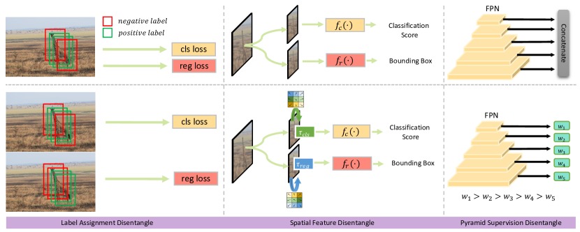
Figure 3. The proposed DDOD consists of 3 parts: label assignment disentanglement, spatial feature disentanglement, and pyramid supervision disentanglement. For each component, our approach (bottom) is compared with the original implementation (top). For label assignment, our method yields different pos/neg labels for the giraffe in classification and regression branches. For spatial feature disentanglement, we propose to learn separate convolutional offset for each branch that aims at providing spatial aligned features for each head. The supervision disentanglement tackles the imbalanced learning problem with different loss weight for each FPN layer where the original one treated all the samples equally.

(1) $$C_{i,\pi(i)}=\underbrace{\mathds{1}\left[\pi(i)\in\Omega_{i}\right]}_{\text{spatial prior}}~{}\cdot~{}\underbrace{{\Bigl{(}\hat{p}_{\pi(i)}(i)\Bigr{)}}^{1-\alpha}}_{\text{classification}}~{}\cdot\underbrace{{\Bigl{(}\mathrm{IoU}\bigl{(}b_{i},\hat{b}_{\pi(i)}(i)\bigr{)}\Bigr{)}}^{\alpha},}_{\text{regression}}$$

where $C_{i,\pi(i)}\in[0,1]$ represents the matching quality of the $\pi(i)$-th prediction with respect to each ground truth, and $\Omega_{i}$ denotes the set of candidate predictions for $i$-th ground truth. To stabilize the training process and make model converge faster, only candidates whose centers fall into the ground-truth boxes are considered as possible foreground samples. In the assignment process, top $K$ predictions with the largest cost value are selected from each FPN level. Then, the candidates are assigned as foreground samples if their matching quality is beyond an adaptive threshold computed with the batch statistics like ATSS.

In order to decouple the label assignment of classification and regression, we introduce a hyper-parameter $\alpha\in[0,1]$ to balance the contribution between them. Intuitively, samples with higher foreground probability should be prioritized for classification, while the regression branch focuses more on regression quality. A detailed ablation study on $\alpha$ will be elaborated in Section 5.4.1. In doing so, classification and regression tasks are disentangled successfully, through which both objectives are achieved in a better way.

4.2. Spatial Feature Disentanglement

Our pilot experiments have shown the difference between the most informative features for classification and regression. Here, we describe a simple but effective approach to spatially disentangle these features with the help of deformable convolution. Similar ideas (Song et al., 2020; Wu et al., 2020a) have been proved successful in two-stage detectors, and here we extend them to dense detectors. The gist is to let the model attend the most important feature for decision-making, but such a disentanglement is somewhat conflict with the parallel head architecture in state-of-the-art dense object detectors. However, with the help of deformable convolution, the model is able to attend different spatial fields in the input feature map using the same number of convolutions. Inspired by this, we introduce the adaptive feature disentanglement module, in which a learnable convolution offset is predicted on each position $p_{n}$ to adaptively select the spatial features for the current task. Formally, for each position $p_{i}$ on the feature map $F$, we have

(2) $$F(p_{i})=\sum_{p_{n}\in\textit{R}}w(p_{n})\cdot x(p_{i}+p_{n}+\Delta p_{n}).$$

Instead of sampling using a regular grid $R$ over the input feature map, we let the model learn the best fitted position $\Delta p_{n}$ to convolute for each task. In this paradigm, the classification branch focuses more on class-wise discriminative features, e.g., the human face of a person or the wheel of a car. On the other hand, the regression branch pays more attention to border features. Since the offset should be correlated with the information at current position, the offset $\Delta p_{n}$ is predicted with additional filters. In the actual implementation, this operation is implemented through deformable convolution (Dai et al., 2017). We directly replace the first convolution with deformable convolution in the classification and regression subnets. Hence, features from FPN can be dynamically extracted given the different tasks at the same time, without competing with each other.

4.3. Pyramid Supervision Disentanglement

Samples located at different levels of feature pyramid are entangled together with equal supervision since the FPN (Lin et al., 2017a) was proposed. However, as described in Section 3.3, this practice does not consider the imbalance contribution of training samples from different layers. Concretely, objects located at $P_{3}$ level receive more attention because of the huge number of training samples on it. On the contrary, objects fall into $P_{7}$ level are less likely to be well-trained due to the lack of training samples. A natural solution to alleviate this phenomenon is to strengthen the supervision in deeper layers. In practice, this can be easily achieved through assigning samples in deeper layers with larger weights. For this purpose, we propose FPN hierarchical loss on top of the original supervision. The reason behind the gradient imbalance issue is the number of samples falling in different layers varies. Therefore, we directly choose the count of samples as the metric to indicate whether we should down-weight/up-weight supervision during training. The re-weighting coefficient $w$ for the sample located on layer $L_{i}$ with respect to the loss $L$ is formulated as:

(3) $$w_{cls} =2-\frac{n_{cls}^{i}-min(N_{cls})}{max(N_{cls})-min(N_{cls})}$$

(4) $$w_{reg} =2-\frac{n_{reg}^{i}-min(N_{reg})}{max(N_{reg})-min(N_{reg})}$$

(5) $$L =w_{cls}\cdot L_{cls}+w_{reg}\cdot L_{reg},$$

where $n_{cls}^{i}$ and $n_{reg}^{i}$ are the number of positive samples located at FPN level $i$ based on the aforementioned classification and regression branches, $N_{cls}$ and $N_{reg}$ are the set of $n_{cls}^{i}$ and $n_{reg}^{i}$ respectively. When the re-weighting factor $w$ ranges from 1.0 to 2.0, we empirically find that samples on $P_{3}$ level always get a factor of 1.0 and those on $P_{7}$ level are always 2.0. From the gradient balance perspective, such results are beneficial for large object learning. Besides, we adopt a moving average manner to relieve the distributional difference of labels among images and stabilize the training process. More specifically, we use the accumulated number of positive samples $\sum_{j=0}^{J}{n^{i}_{cls/reg}}$ at each FPN level $i$ until current iteration $J$ to compute $w$.

5. Experiments

Table 3. Comparison of detection AP results on different single-stage object detectors (RetinaNet, FCOS, and ATSS).

Model	DDOD	AP	AP50	AP75	APS	APM	APL
RetinaNet		36.5	55.4	39.1	20.4	40.3	48.1
RetinaNet	✓	38.5	58.1	41.2	20.7	41.4	51.6
FCOS *		39.2	57.3	42.4	22.7	43.1	51.5
FCOS *	✓	41.6	59.7	45.3	24.3	45.0	55.1
ATSS		39.4	56.6	42.6	23.9	42.5	49.6
ATSS	✓	41.6	59.9	45.2	23.9	44.9	54.4

• The advanced version of FCOS implementation in ATSS is adopted.

Table 4. Effects of each component in our DDOD. Results are reported on COCO val-2017 with ATSS.

Assignment Disentangle	Spatial Feature Disentangle	Supervision Disentangle	AP	AP50	AP75	APS	APM	APL
			39.4	56.6	42.6	23.9	42.5	49.6
✓			40.4	58.9	43.8	24.1	43.9	51.4
	✓		40.6	58.6	44.1	24.0	44.1	52.5
		✓	40.0	57.9	43.1	23.0	43.6	52.6
✓	✓	✓	41.6	59.9	45.2	23.9	44.9	54.4

In this section, we construct extensive experiments on COCO (Lin et al., 2014) and WIDER FACE (Yang et al., 2016) datasets to study the proposed DDOD. We first present the effectiveness and generality of our method. Secondly, we show the ablation results of different modules. Thirdly, we conduct experiments to discuss some interesting aspects to gain deeper insight of the proposed DDOD. Finally, we compare our approach with other state-of-the-art models and show our superiority.

Table 5. AP performance with different $\alpha$ for classification and regression label assignment strategies.

	0.5	0.6	0.7	0.8
0.5	39.4	39.3	39.0	39.0
0.6	39.6	39.4	39.5	39.5
0.7	39.9	40.1	39.7	39.6
0.8	40.4	40.0	40.0	39.9

5.1. Implementation Details

Most experiments are carried out on COCO benchmark, where we train the model on trainval35k with 115K images and report performance on minval with 5K images. Besides, we report the final results on test-dev with 20K images from the evaluation server. Except for the results on test-dev, all experiments are trained under standard 1x schedule setting based on ResNet-50 (He et al., 2016), with default parameters adopted in MMDetection (Chen et al., 2019b). Moreover, in order to adapt cost function-based label assignment, we replace the centerness branch with IoU-prediction branch. In addition to COCO, we also validate our approach on WIDER FACE, which is currently the largest face detection dataset. The model is trained with a batch size of 24 on 6 Titan V100s. The schedule of learning rate is annealing down from 7.5e-3 to 7.5e-5 every 30 epochs using cosine decay rule. This process is repeated for 20 times, indicating a total epoch number of 600. In order to align our baseline with other face detectors, deformable convolution block, SSH module, and DIoU loss are adopted.

5.2. Results on Dense Object Detectors

We implement DDOD on three different representative dense detectors: RetinaNet, FCOS, and ATSS. The mAP performance is reported in Table 3. Our DDOD boosts all the baselines by more than 2.0 mAP, which validates the effectiveness and generation ability of the proposed method. When observing the results in detail, we find that the AP_L is promoted most in all three detectors. The reasons can be two-fold. Firstly, large objects are more prominent in the image plain, so our spatial disentangle module is easier to attend important parts. Secondly, Our FPN hierarchical loss is proposed to compensate for the insufficient supervision for high level feature maps, so the mAP for large objects is directly benefited.

Table 6. AP performance with different positions of deformable convolution in classification and regression heads.

Position	AP	AP50	AP75	APS	APM	APL
1	40.6	58.4	44.3	23.6	44.3	52.4
2	40.3	58.5	44.1	23.9	44.0	52.4
3	40.1	57.9	43.4	23.0	44.6	52.4
4	40.1	57.9	43.1	23.0	44.6	52.6

Table 7. AP performance with various re-weighting strategies for FPN hierarchical loss.

Method	AP	AP50	AP75	APS	APM	APL
Sum-Reweight	39.7	57.5	43.2	22.6	43.3	52.1
Sum-Reweight*	39.8	57.8	43.1	23.0	43.3	51.0
Linear-Reweight	39.8	57.8	42.9	22.9	43.5	51.8
Linear-Reweight*	39.8	57.7	42.9	23.0	43.5	52.0
Linear-Interpolate	39.8	57.9	43.1	23.1	43.2	51.1
Linear-Interpolate*	40.0	57.9	43.4	22.9	43.6	52.6

• indicates the implementation of moving average version by counting all valid samples till current iteration.

5.3. Ablation Study

To understand how each disentanglement in DDOD facilitates detection performance, we test each component independently on the baseline detector ATSS and report its AP performance in Table 4. The overall AP of the baseline starts from 39.4. When label assignment disentanglement is applied, the AP is raised by 1.0 and the improvement is seen on objects of all sizes. This result vindicates our findings in Section 4.1 that decoupling the encoding conjunctions between classification and bounding box regression is necessary. Then, we add the spatial feature disentanglement that brings us an 1.2 AP enhancement. Specifically, the AP_L is benefited most, which validates our first assumption in Section 4.2. Another interesting finding is that the improvement on AP₇₅ brought by spatial feature disentanglement achieves 1.5, suggesting the underlying connection between correctly attending receptive regions and accurate bounding box localization. When pyramid supervision disentanglement is added, the accuracy is promoted by 0.6 and the AP_L is raised by 3.0. This large improvement is in correspondence with our analysis in Section 4.3 and the underlying intuition of this disentanglement. Finally, the AP achieves 41.6 when all three disentanglement are applied, gaining an 2.2 absolute improvement and validating our approach.

Method	Backbone	Epoch	MS${}_{\text{train}}$	FPS	AP	AP50	AP75	APS	APM	APL	Reference
multi-stage:
Faster R-CNN w/ FPN (Lin et al., 2017a)	R-101	24		14.2	36.2	59.1	39.0	18.2	39.0	48.2	CVPR17
Cascade R-CNN (Cai and Vasconcelos, 2018)	R-101	18		11.9	42.8	62.1	46.3	23.7	45.5	55.2	CVPR18
Grid R-CNN (Lu et al., 2019)	R-101	20		11.4	41.5	60.9	44.5	23.3	44.9	53.1	CVPR19
Libra R-CNN (Pang et al., 2019)	X-101-64x4d	12		8.5	43.0	64.0	47.0	25.3	45.6	54.6	CVPR19
RepPoints (Yang et al., 2019)	R-101	24		13.3	41.0	62.9	44.3	23.6	44.1	51.7	ICCV19
RepPoints (Yang et al., 2019)	R-101-DCN	24	$\checkmark$	11.8	45.0	66.1	49.0	26.6	48.6	57.5	ICCV19
RepPointsV2 (Chen et al., 2020)	R-101	24	$\checkmark$	11.1	46.0	65.3	49.5	27.4	48.9	57.3	NeurIPS20
RepPointsV2 (Chen et al., 2020)	R-101-DCN	24	$\checkmark$	10.0	48.1	67.5	51.8	28.7	50.9	60.8	NeurIPS20
TridentNet (Li et al., 2019a)	R-101	24	$\checkmark$	2.7	42.7	63.6	46.5	23.9	46.6	56.6	ICCV19
TridentNet (Li et al., 2019a)	R-101-DCN	36	$\checkmark$	1.3	46.8	67.6	51.5	28.0	51.2	60.5	ICCV19
TSD (Song et al., 2020)	R-101	20		1.1	43.2	64.0	46.9	24.0	46.3	55.8	CVPR20
BorderDet (Qiu et al., 2020)	R-101	24	$\checkmark$	13.2	45.4	64.1	48.8	26.7	48.3	56.5	ECCV20
BorderDet (Qiu et al., 2020)	X-101-64x4d	24	$\checkmark$	8.1	47.2	66.1	51.0	28.1	50.2	59.9	ECCV20
BorderDet (Qiu et al., 2020)	X-101-64x4d-DCN	24	$\checkmark$	6.4	48.0	67.1	52.1	29.4	50.7	60.5	ECCV20
one-stage:
TPNet320 (Wang and Zhang, 2020)	R-101	24		25.7	34.2	53.1	36.4	13.6	36.8	50.5	ACM MM20
TPNet512 (Wang and Zhang, 2020)	R-101	24		13.9	39.6	58.5	42.8	20.5	45.3	53.3	ACM MM20
CornerNet (Law and Deng, 2018)	HG-104	200	$\checkmark$	3.1	40.6	56.4	43.2	19.1	42.8	54.3	ECCV18
CenterNet (Duan et al., 2019)	HG-104	190	$\checkmark$	3.3	44.9	62.4	48.1	25.6	47.4	57.4	ICCV19
CentripetalNet (Dong et al., 2020)	HG-104	210	$\checkmark$	n/a	45.8	63.0	49.3	25.0	48.2	58.7	CVPR20
RetinaNet (Lin et al., 2017b)	R-101	18		13.6	39.1	59.1	42.3	21.8	42.7	50.2	ICCV17
FreeAnchor (Zhang et al., 2019b)	R-101	24	$\checkmark$	12.8	43.1	62.2	46.4	24.5	46.1	54.8	NeurIPS19
FreeAnchor (Zhang et al., 2019b)	X-101-32x8d	24	$\checkmark$	8.2	44.9	64.3	48.5	26.8	48.3	55.9	NeurIPS19
FSAF (Zhu et al., 2019)	R-101	18	$\checkmark$	15.1	40.9	61.5	44.0	24.0	44.2	51.3	CVPR19
FSAF (Zhu et al., 2019)	X-101-64x4d	18	$\checkmark$	9.1	42.9	63.8	46.3	26.6	46.2	52.7	CVPR19
FCOS (Tian et al., 2019)	R-101	24	$\checkmark$	14.7	41.5	60.7	45.0	24.4	44.8	51.6	ICCV19
FCOS (Tian et al., 2019)	X-101-64x4d	24	$\checkmark$	8.9	44.7	64.1	48.4	27.6	47.5	55.6	ICCV19
SAPD (Zhu et al., 2020b)	R-101	24	$\checkmark$	13.2	43.5	63.6	46.5	24.9	46.8	54.6	CVPR20
SAPD (Zhu et al., 2020b)	R-101-DCN	24	$\checkmark$	11.1	46.0	65.9	49.6	26.3	49.2	59.6	CVPR20
SAPD (Zhu et al., 2020b)	X-101-32x4d-DCN	24	$\checkmark$	8.8	46.6	66.6	50.0	27.3	49.7	60.7	CVPR20
ATSS (Zhang et al., 2020b)	R-101	24	$\checkmark$	14.6	43.6	62.1	47.4	26.1	47.0	53.6	CVPR20
ATSS (Zhang et al., 2020b)	R-101-DCN	24	$\checkmark$	12.7	46.3	64.7	50.4	27.7	49.8	58.4	CVPR20
ATSS (Zhang et al., 2020b)	X-101-32x8d-DCN	24	$\checkmark$	6.9	47.7	66.6	52.1	29.3	50.8	59.7	CVPR20
PAA (Kim and Lee, 2020)	R-101	24	$\checkmark$	14.6	44.8	63.3	48.7	26.5	48.8	56.3	ECCV20
PAA (Kim and Lee, 2020)	R-101-DCN	24	$\checkmark$	12.7	47.4	65.7	51.6	27.9	51.3	60.6	ECCV20
PAA (Kim and Lee, 2020)	X-101-64x4d-DCN	24	$\checkmark$	6.9	49.0	67.8	53.3	30.2	52.8	62.2	ECCV20
GFL (Li et al., 2020)	R-50	24	$\checkmark$	19.4	43.1	62.0	46.8	26.0	46.7	52.3	NeurIPS20
GFL (Li et al., 2020)	R-101	24	$\checkmark$	14.6	45.0	63.7	48.9	27.2	48.8	54.5	NeurIPS20
GFL (Li et al., 2020)	R-101-DCN	24	$\checkmark$	12.7	47.3	66.3	51.4	28.0	51.1	59.2	NeurIPS20
GFL (Li et al., 2020)	X-101-32x4d-DCN	24	$\checkmark$	10.7	48.2	67.4	52.6	29.2	51.7	60.2	NeurIPS20
DDOD (ours)	R-50	24	$\checkmark$	18.6	45.0	63.5	49.3	27.2	47.9	55.9	–
DDOD (ours)	R-101	24	$\checkmark$	14.0	46.7	65.3	51.1	28.2	49.9	57.9	–
DDOD (ours)	R-101-DCN	24	$\checkmark$	12.0	49.0	67.7	53.6	29.6	52.2	62.3	–
DDOD (ours)	X-101-32x4d-DCN	24	$\checkmark$	10.3	50.1	69.0	54.8	30.8	53.5	63.2	–
DDOD (ours)	R2-101-DCN	24	$\checkmark$	10.4	51.2	69.9	55.9	32.2	54.4	64.9	–
DDOD-X (ours)	R2-101-DCN	24	$\checkmark$	8.4	52.5	71.0	57.2	33.9	56.8	65.9	–
DDOD-X (ours) + MS${}_{\text{test}}$	R2-101-DCN	24	$\checkmark$	-	55.0	72.6	60.0	37.0	58.0	66.7	–

Table 8. Comparisons between state-of-the-art detectors on COCO test-dev (single-model and single-scale results except for the last row). “MS${}_{\text{train}}$” and “MS${}_{\text{test}}$” denote multi-scale training and testing, respectively; FPS values are measured on a single NVIDIA Titan V100 machine, using a batch size of 1 whenever possible; “n/a” means that both trained models and timing results from original papers are not available; R: ResNet (He et al., 2016); X: ResNeXt (Xie et al., 2017); HG: Hourglass (Newell et al., 2016); DCN: Deformable Convolutional Network (Dai et al., 2017); R2: Res2Net (Gao et al., 2021).

Table 9. AP performance of different methods on WIDER FACE val subset. Our DDOD-Face achieves state-of-the-art results on AP hard under the same single-model test setting.

Method	Backbone	Easy	Medium	Hard
PyramidBox (Tang et al., 2018)	VGG-16	0.961	0.950	0.889
PyramidBox++ (Li et al., 2019b)	VGG-16	0.967	0.959	0.912
AInnoFace (Zhang et al., 2019a)	ResNet-152	0.970	0.961	0.918
RetinaFace (Deng et al., 2019)	ResNet-152	0.969	0.961	0.918
RefineFace (Zhang et al., 2020a)	ResNet-152	0.972	0.962	0.920
DSFD (Li et al., 2019c)	ResNet-152	0.966	0.957	0.904
ASFD-D6 (Zhang et al., 2020c)	ResNet-152	0.972	0.965	0.925
HAMBox (Liu et al., 2020)	ResNet-50	0.970	0.964	0.933
TinaFace (Zhu et al., 2020a)	ResNet-50	0.970	0.963	0.934
ATSS	ResNet-50	0.964	0.958	0.930
DDOD-Face (ours)	ResNet-50	0.970	0.964	0.935

5.4. Discussion

In this section, we delve into our DDOD to study how the mAP improvements are actually achieved and to gain deeper understanding of the underlying mechanisms. For all experiments, we employ ResNet-50-based ATSS with the same settings in Section 5.1.

5.4.1. What is the Best Label Assignment Disentanglement?

We conduct experiments to investigate the optimal strategy for our encoding disentanglement, i.e., to find the best $\alpha$ for classification and regression respectively. As presented in Table 5, the results are quite straight-forward: for regression branch, $\alpha=0.5$ works better, while $\alpha=0.8$ works best for classification. Although one extra hyper-parameter is introduced for label assignment, we find this setting ($\alpha_{cls}=0.8,\alpha_{reg}=0.5$) is robust to other scenarios when applying it on WIDER FACE dataset. The difference between optimal $\alpha$ values validates that the classification and regression branches should have their own label assignment criteria. We also observe that increasing $\alpha_{cls}$ will benefit the accuracy, suggesting that the IoU between anchors and ground-truth boxes are decisive for setting classification target. On the other hand, decreasing $\alpha_{reg}$ is good for the AP performance, indicating that the regression encoding should take the real-time classification results into consideration.

5.4.2. Optimal Spatial Feature Disentanglement under Given Computational Budget.

Empirically, replacing some convolution operations with deformable convolution can somewhat bring performance enhancement, but seeking the best way for such replacement is nontrivial, as we want to avoid unbearable extra computational cost and the optimization difficulty brought by to many DCN layers. Hence, we only replace one convolution with DCN in each branch, and study the optimal way for the replacement. Concretely, we carry out experiments by replacing each convolution with its deformable version independently and check the final performance. From Table 6, we find that disentangling feature representation at the first stage works best, with 40.6 mAP on COCO validation set. An interesting phenomenon is that the overall performance decrease when moving feature disentanglement to the latter layer in detection heads, indicating that disentangling features directly from FPN eases the learning process.

5.4.3. Seeking the Most Robust Re-weighting Strategy.

In this part, we examine different re-weighting schemes to show that our proposed linear-interpolation re-weighting works best. The ablation results are shown in Table 7. Firstly, we test the Linear-Reweight proposed in (Yang et al., 2021), in which the factors that linearly increase from 1.0 to 2.0 are assigned to each FPN level. Secondly, considering that most negative samples are greatly suppressed by the focal loss, we propose a vanilla re-weight strategy where the weight of each FPN layer is proportionate to the number of positive samples, which is denoted as Sum-Reweight. Additionally, since the number of positive samples can vary greatly according to the input batch, we extend the Linear-Reweight, Sum-Reweight, and our proposed Linear-Interpolate to that the weights are moving-averaged during optimization. This extension can stabilize the training process and slightly improve the accuracy according to Table 7. From the results, we can conclude that our linear-interpolation beats the other two policies, achieving 40.0 mAP on COCO val subset.

5.5. Comparison with State-of-the-Arts

As shown in Table 8, we compare DDOD with state-of-the-art methods on COCO test-dev. Following the common practice, we adopt multi-scale training to improve model robustness. For fair comparison, results with single-model and single-scale testing at a short side of 800 are reported. When using the same backbone network, our DDOD beats all other methods including the recently developed GFL (Li et al., 2020) and PAA (Kim and Lee, 2020). Additionally, empowered by the advanced Res2Net-101-DCN backbone, DDOD achieves a suppressing 52.5 mAP in the single-scale testing protocol, suggesting its great prospect in various applications. Finally, we incorporate techniques like multi-scale testing, Soft-NMS and stronger data augmentation for further performance improvement, achieving 55.0 mAP, which establishes new state-of-the-art performance on this competitive benchmark.

5.6. Results on WIDER FACE Dataset

In addition to general object detection, our method is also applicable in other scenarios like face detection. We evaluate DDOD on the WIDER FACE benchmark, the currently largest open-sourced face detection dataset. It provides many difficult and realistic scenes with the varieties of occlusion, scale, and illumination. In those complex and crowded scenes, our model is quite robust and even outperforms several detectors designed for face detection, as shown in Table 9. In order to get better performance on WIDER FACE, which is different from COCO, we adopt DCN (Dai et al., 2017), SSH module (Najibi et al., 2017), and DIoU loss (Zheng et al., 2020) on original ATSS model, reaching an overall AP of 93.0. Though this result surpasses several competitive face detectors, DDOD is still able to improve it by approximately 0.5 AP under easy, medium and, hard settings. More importantly, our DDOD-Face with ResNet-50 backbone achieves 97.0%, 96.4%, 93.5% in these three settings on the validation subset, reaching state-of-the-art result on AP hard under the same single-model test setting.

6. Conclusion

In this work, we develop the DDOD, a new training paradigm for dense object detectors. DDOD decomposes conjunctions lying in most current one-stage detectors via label assignment disentanglement, spatial feature disentanglement, and pyramid supervision disentanglement. The findings in this paper can potentially be harnessed to improve the detection accuracy and applied on various dense object detectors. We have demonstrated that DDOD achieves state-of-the-art results on COCO and WIDER FACE benchmarks, and validated its effectiveness and generalization as well. Furthermore, our approach may help to improve the performance of two-stage detectors. Therefore, how to embed DDOD into RCNN-like detectors will be an important next step to generalize DDOD.

References

- (1)
- Bochkovskiy et al. (2020) Alexey Bochkovskiy, Chien-Yao Wang, and Hong-Yuan Mark Liao. 2020. YOLOv4: Optimal speed and accuracy of object detection. arXiv preprint arXiv:2004.10934 (2020).
- Cai and Vasconcelos (2018) Zhaowei Cai and Nuno Vasconcelos. 2018. Cascade RCNN: Delving into high quality object detection. In Proceedings of the IEEE/CVF Conference on Computer Vision and Pattern Recognition.
- Chen et al. (2019b) Kai Chen, Jiaqi Wang, Jiangmiao Pang, Yuhang Cao, Yu Xiong, Xiaoxiao Li, Shuyang Sun, Wansen Feng, Ziwei Liu, Jiarui Xu, et al. 2019b. MMDetection: Open mmlab detection toolbox and benchmark. arXiv preprint arXiv:1906.07155 (2019).
- Chen et al. (2019a) Yuntao Chen, Chenxia Han, Naiyan Wang, and Zhaoxiang Zhang. 2019a. Revisiting feature alignment for one-stage object detection. arXiv preprint arXiv:1908.01570 (2019).
- Chen et al. (2020) Yihong Chen, Zheng Zhang, Yue Cao, Liwei Wang, Stephen Lin, and Han Hu. 2020. Reppoints v2: Verification meets regression for object detection. Advances in Neural Information Processing Systems 33 (2020).
- Dai et al. (2017) Jifeng Dai, Haozhi Qi, Yuwen Xiong, Yi Li, Guodong Zhang, Han Hu, and Yichen Wei. 2017. Deformable convolutional networks. In Proceedings of the IEEE international conference on computer vision. 764–773.
- Deng et al. (2009) Jia Deng, Wei Dong, Richard Socher, Li-Jia Li, Kai Li, and Li Fei-Fei. 2009. Imagenet: A large-scale hierarchical image database. In Proceedings of the IEEE/CVF Conference on Computer Vision and Pattern Recognition. 248–255.
- Deng et al. (2019) Jiankang Deng, Jia Guo, Yuxiang Zhou, Jinke Yu, Irene Kotsia, and Stefanos Zafeiriou. 2019. Retinaface: Single-stage dense face localisation in the wild. arXiv preprint arXiv:1905.00641 (2019).
- Dong et al. (2020) Zhiwei Dong, Guoxuan Li, Yue Liao, Fei Wang, Pengju Ren, and Chen Qian. 2020. Centripetalnet: Pursuing high-quality keypoint pairs for object detection. In Proceedings of the IEEE/CVF Conference on Computer Vision and Pattern Recognition. 10519–10528.
- Duan et al. (2019) Kaiwen Duan, Song Bai, Lingxi Xie, Honggang Qi, Qingming Huang, and Qi Tian. 2019. Centernet: Keypoint triplets for object detection. In Proceedings of the IEEE International Conference on Computer Vision.
- Gao et al. (2021) Shanghua Gao, Ming-Ming Cheng, Kai Zhao, Xin-Yu Zhang, Ming-Hsuan Yang, and Philip HS Torr. 2021. Res2Net: A New Multi-Scale Backbone Architecture. IEEE Transactions on Pattern Analysis and Machine Intelligence 43, 2 (2021), 652–662. https://doi.org/10.1109/TPAMI.2019.2938758
- Girshick et al. (2014) Ross Girshick, Jeff Donahue, Trevor Darrell, and Jitendra Malik. 2014. Rich feature hierarchies for accurate object detection and semantic segmentation. In Proceedings of the IEEE/CVF Conference on Computer Vision and Pattern Recognition.
- He et al. (2016) Kaiming He, Xiangyu Zhang, Shaoqing Ren, and Jian Sun. 2016. Deep residual learning for image recognition. In Proceedings of the IEEE/CVF Conference on Computer Vision and Pattern Recognition.
- Huang et al. (2015) Lichao Huang, Yi Yang, Yafeng Deng, and Yinan Yu. 2015. DenseBox: Unifying landmark localization with end to end object detection. arXiv preprint arXiv:1509.04874 (2015).
- Jiang et al. (2018) Borui Jiang, Ruixuan Luo, Jiayuan Mao, Tete Xiao, and Yuning Jiang. 2018. Acquisition of localization confidence for accurate object detection. In Proceedings of the European Conference on Computer Vision. 784–799.
- Kim and Lee (2020) Kang Kim and Hee Seok Lee. 2020. Probabilistic anchor assignment with iou prediction for object detection. arXiv preprint arXiv:2007.08103 (2020).
- Law and Deng (2018) Hei Law and Jia Deng. 2018. CornerNet: Detecting objects as paired keypoints. In Proceedings of the European Conference on Computer Vision.
- Li et al. (2019c) Jian Li, Yabiao Wang, Changan Wang, Ying Tai, Jianjun Qian, Jian Yang, Chengjie Wang, Jilin Li, and Feiyue Huang. 2019c. DSFD: dual shot face detector. In Proceedings of the IEEE/CVF Conference on Computer Vision and Pattern Recognition. 5060–5069.
- Li et al. (2020) Xiang Li, Wenhai Wang, Lijun Wu, Shuo Chen, Xiaolin Hu, Jun Li, Jinhui Tang, and Jian Yang. 2020. Generalized Focal Loss: Learning Qualified and Distributed Bounding Boxes for Dense Object Detection. In Advances in Neural Information Processing Systems.
- Li et al. (2019a) Yanghao Li, Yuntao Chen, Naiyan Wang, and Zhaoxiang Zhang. 2019a. Scale-aware trident networks for object detection. In Proceedings of the IEEE International Conference on Computer Vision.
- Li et al. (2019b) Zhihang Li, Xu Tang, Junyu Han, Jingtuo Liu, and Ran He. 2019b. Pyramidbox++: High performance detector for finding tiny face. arXiv preprint arXiv:1904.00386 (2019).
- Lin et al. (2017a) Tsung-Yi Lin, Piotr Dollár, Ross Girshick, Kaiming He, Bharath Hariharan, and Serge Belongie. 2017a. Feature pyramid networks for object detection. In Proceedings of the IEEE/CVF Conference on Computer Vision and Pattern Recognition.
- Lin et al. (2017b) Tsung-Yi Lin, Priya Goyal, Ross Girshick, Kaiming He, and Piotr Dollár. 2017b. Focal loss for dense object detection. In Proceedings of the IEEE International Conference on Computer Vision.
- Lin et al. (2014) Tsung-Yi Lin, Michael Maire, Serge Belongie, James Hays, Pietro Perona, Deva Ramanan, Piotr Dollár, and C Lawrence Zitnick. 2014. Microsoft coco: Common objects in context. In Proceedings of the European Conference on Computer Vision.
- Liu et al. (2020) Yang Liu, Xu Tang, Junyu Han, Jingtuo Liu, Dinger Rui, and Xiang Wu. 2020. HAMBox: Delving Into Mining High-Quality Anchors on Face Detection. In IEEE/CVF Conference on Computer Vision and Pattern Recognition.
- Lu et al. (2019) Xin Lu, Buyu Li, Yuxin Yue, Quanquan Li, and Junjie Yan. 2019. Grid R-CNN. In Proceedings of the IEEE/CVF Conference on Computer Vision and Pattern Recognition.
- Najibi et al. (2017) Mahyar Najibi, Pouya Samangouei, Rama Chellappa, and Larry S Davis. 2017. Ssh: Single stage headless face detector. In Proceedings of the IEEE International Conference on Computer Vision. 4875–4884.
- Najibi et al. (2019) Mahyar Najibi, Bharat Singh, and Larry S Davis. 2019. Autofocus: Efficient multi-scale inference. In Proceedings of the IEEE International Conference on Computer Vision.
- Newell et al. (2016) Alejandro Newell, Kaiyu Yang, and Jia Deng. 2016. Stacked hourglass networks for human pose estimation. In Proceedings of the European Conference on Computer Vision. Springer, 483–499.
- Oksuz et al. (2020) Kemal Oksuz, Baris Can Cam, Sinan Kalkan, and Emre Akbas. 2020. Imbalance problems in object detection: A review. IEEE Transactions on Pattern Analysis and Machine Intelligence (2020).
- Pang et al. (2019) Jiangmiao Pang, Kai Chen, Jianping Shi, Huajun Feng, Wanli Ouyang, and Dahua Lin. 2019. Libra r-cnn: Towards balanced learning for object detection. In Proceedings of the IEEE/CVF Conference on Computer Vision and Pattern Recognition.
- Qiu et al. (2020) Han Qiu, Yuchen Ma, Zeming Li, Songtao Liu, and Jian Sun. 2020. Borderdet: Border Feature for Dense Object Detection. In Proceedings of the European Conference on Computer Vision.
- Ren et al. (2015) Shaoqing Ren, Kaiming He, Ross Girshick, and Jian Sun. 2015. Faster r-cnn: Towards real-time object detection with region proposal networks. In Advances in Neural Information Processing Systems.
- Song et al. (2020) Guanglu Song, Yu Liu, and Xiaogang Wang. 2020. Revisiting the sibling head in object detector. In Proceedings of the IEEE/CVF Conference on Computer Vision and Pattern Recognition. 11563–11572.
- Sun et al. (2020) Peize Sun, Yi Jiang, Enze Xie, Zehuan Yuan, Changhu Wang, and Ping Luo. 2020. OneNet: Towards End-to-End One-Stage Object Detection. arXiv preprint arXiv:2012.05780 (2020).
- Tan et al. (2020a) Jingru Tan, Xin Lu, Gang Zhang, Changqing Yin, and Quanquan Li. 2020a. Equalization Loss v2: A New Gradient Balance Approach for Long-tailed Object Detection. arXiv preprint arXiv:2012.08548 (2020).
- Tan et al. (2020b) Jingru Tan, Changbao Wang, Buyu Li, Quanquan Li, Wanli Ouyang, Changqing Yin, and Junjie Yan. 2020b. Equalization loss for long-tailed object recognition. In Proceedings of the IEEE/CVF Conference on Computer Vision and Pattern Recognition. 11662–11671.
- Tang et al. (2018) Xu Tang, Daniel K Du, Zeqiang He, and Jingtuo Liu. 2018. Pyramidbox: A context-assisted single shot face detector. In Proceedings of the European Conference on Computer Vision. 797–813.
- Tian et al. (2019) Zhi Tian, Chunhua Shen, Hao Chen, and Tong He. 2019. Fcos: Fully convolutional one-stage object detection. In Proceedings of the IEEE International Conference on Computer Vision.
- Vu et al. (2019) Thang Vu, Hyunjun Jang, Trung X. Pham, and Chang Yoo. 2019. Cascade RPN: Delving into High-Quality Region Proposal Network with Adaptive Convolution. In Advances in Neural Information Processing Systems, Vol. 32. Curran Associates, Inc.
- Wang et al. (2020a) Chien-Yao Wang, Alexey Bochkovskiy, and Hong-Yuan Mark Liao. 2020a. Scaled-YOLOv4: Scaling Cross Stage Partial Network. arXiv preprint arXiv:2011.08036 (2020).
- Wang et al. (2019) Jiaqi Wang, Kai Chen, Shuo Yang, Chen Change Loy, and Dahua Lin. 2019. Region proposal by guided anchoring. In Proceedings of the IEEE/CVF Conference on Computer Vision and Pattern Recognition.
- Wang et al. (2020b) Jianfeng Wang, Lin Song, Zeming Li, Hongbin Sun, Jian Sun, and Nanning Zheng. 2020b. End-to-end object detection with fully convolutional network. arXiv preprint arXiv:2012.03544 (2020).
- Wang et al. (2020c) Jiaqi Wang, Wenwei Zhang, Yuhang Cao, Kai Chen, Jiangmiao Pang, Tao Gong, Jianping Shi, Chen Change Loy, and Dahua Lin. 2020c. Side-aware boundary localization for more precise object detection. Proceedings of the European Conference on Computer Vision (2020).
- Wang and Zhang (2020) Keyang Wang and Lei Zhang. 2020. Single-Shot Two-Pronged Detector with Rectified IoU Loss. In Proceedings of the 28th ACM International Conference on Multimedia (Seattle, WA, USA) (MM ’20). New York, NY, USA, 1311–1319.
- Wu et al. (2020b) Jialian Wu, Liangchen Song, Tiancai Wang, Qian Zhang, and Junsong Yuan. 2020b. Forest r-cnn: Large-vocabulary long-tailed object detection and instance segmentation. In Proceedings of the 28th ACM International Conference on Multimedia. 1570–1578.
- Wu et al. (2020a) Yue Wu, Yinpeng Chen, Lu Yuan, Zicheng Liu, Lijuan Wang, Hongzhi Li, and Yun Fu. 2020a. Rethinking Classification and Localization for Object Detection. In Proceedings of the IEEE/CVF Conference on Computer Vision and Pattern Recognition.
- Xie et al. (2017) Saining Xie, Ross Girshick, Piotr Dollár, Zhuowen Tu, and Kaiming He. 2017. Aggregated Residual Transformations for Deep Neural Networks. In Proceedings of the IEEE/CVF Conference on Computer Vision and Pattern Recognition.
- Yang et al. (2021) Chenhongyi Yang, Zehao Huang, and Naiyan Wang. 2021. QueryDet: Cascaded Sparse Query for Accelerating High-Resolution Small Object Detection. arXiv preprint arXiv:2103.09136 (2021).
- Yang et al. (2016) Shuo Yang, Ping Luo, Chen-Change Loy, and Xiaoou Tang. 2016. Wider face: A face detection benchmark. In Proceedings of the IEEE Conference on Computer Vision and Pattern Recognition. 5525–5533.
- Yang et al. (2019) Ze Yang, Shaohui Liu, Han Hu, Liwei Wang, and Stephen Lin. 2019. Reppoints: Point set representation for object detection. In Proceedings of the IEEE International Conference on Computer Vision.
- Zhang et al. (2020c) Bin Zhang, Jian Li, Yabiao Wang, Ying Tai, Chengjie Wang, Jilin Li, Feiyue Huang, Yili Xia, Wenjiang Pei, and Rongrong Ji. 2020c. ASFD: Automatic and Scalable Face Detector. arXiv preprint arXiv:2003.11228 (2020).
- Zhang et al. (2019a) Faen Zhang, Xinyu Fan, Guo Ai, Jianfei Song, Yongqiang Qin, and Jiahong Wu. 2019a. Accurate face detection for high performance. arXiv preprint arXiv:1905.01585 (2019).
- Zhang et al. (2020a) Shifeng Zhang, Cheng Chi, Zhen Lei, and Stan Z Li. 2020a. Refineface: Refinement neural network for high performance face detection. IEEE Transactions on Pattern Analysis and Machine Intelligence (2020).
- Zhang et al. (2020b) Shifeng Zhang, Cheng Chi, Yongqiang Yao, Zhen Lei, and Stan Z Li. 2020b. Bridging the gap between anchor-based and anchor-free detection via adaptive training sample selection. In Proceedings of the IEEE/CVF Conference on Computer Vision and Pattern Recognition.
- Zhang et al. (2019b) Xiaosong Zhang, Fang Wan, Chang Liu, Rongrong Ji, and Qixiang Ye. 2019b. FreeAnchor: Learning to Match Anchors for Visual Object Detection. In Advances in Neural Information Processing Systems, Vol. 32.
- Zhang et al. (2021) Xiaosong Zhang, Fang Wan, Chang Liu, Xiangyang Ji, and Qixiang Ye. 2021. Learning to match anchors for visual object detection. IEEE Transactions on Pattern Analysis and Machine Intelligence (2021).
- Zheng et al. (2020) Zhaohui Zheng, Ping Wang, Wei Liu, Jinze Li, Rongguang Ye, and Dongwei Ren. 2020. Distance-IoU loss: Faster and better learning for bounding box regression. In Proceedings of the AAAI Conference on Artificial Intelligence, Vol. 34. 12993–13000.
- Zhou et al. (2018) Bolei Zhou, Yiyou Sun, David Bau, and Antonio Torralba. 2018. Interpretable basis decomposition for visual explanation. In Proceedings of the European Conference on Computer Vision. 119–134.
- Zhu et al. (2020b) Chenchen Zhu, Fangyi Chen, Zhiqiang Shen, and Marios Savvides. 2020b. Soft anchor-point object detection. Proceedings of the European Conference on Computer Vision (2020).
- Zhu et al. (2019) Chenchen Zhu, Yihui He, and Marios Savvides. 2019. Feature selective anchor-free module for single-shot object detection. In Proceedings of the IEEE/CVF Conference on Computer Vision and Pattern Recognition.
- Zhu et al. (2020a) Yanjia Zhu, Hongxiang Cai, Shuhan Zhang, Chenhao Wang, and Yichao Xiong. 2020a. TinaFace: Strong but Simple Baseline for Face Detection. arXiv preprint arXiv:2011.13183 (2020).